MARI – First Consultation · - 0 - MARI – First Consultation Call For Input Abstract This...
109
- 0 - MARI – First Consultation Call For Input Abstract This document provides details on the options of the European mFRR platfrom design, which are consulted from 21 November 2017 – 20 December 2017
Transcript of MARI – First Consultation · - 0 - MARI – First Consultation Call For Input Abstract This...

- 0 -
MARI – First ConsultationCall For Input
AbstractThis document provides details on the options of the European mFRR platfrom design, which
are consulted from 21 November 2017 – 20 December 2017

- 1 -
Table of Content
Introduction ...............................................................................................................4
1.1 Consultation Background ......................................................................................41.2 Document Structure ..............................................................................................6
Product and Process ...................................................................................................7
2.1 Product Properties ................................................................................................72.1.1 Key Characteristics of the Product..................................................................................... 72.1.2 Relation between the Shape of Product and the Shape of Cross-Border Exchange ............. 82.1.3 Options and analysis ......................................................................................................... 92.1.4 Questions ....................................................................................................................... 12
2.2 Process ................................................................................................................ 122.2.1 Introduction ................................................................................................................... 122.2.2 Options .......................................................................................................................... 142.2.3 Analysis .......................................................................................................................... 14
2.2.3.1 The Process of Direct Activations ................................................................................................ 142.2.3.1.1 Base Case: Direct Activation in a Continuous Manner ................................................................................ 142.2.3.1.2 Alternative Option: Direct Activation in Cycles............................................................................................ 152.2.3.1.3 Minimum Distance between Cycles ............................................................................................................. 16
2.2.3.2 The Interaction between the Direct and the Scheduled Process .................................................. 17
2.2.3.3 Evaluation of Alternatives for the mFRR Activation Process ......................................................... 202.2.4 Questions ....................................................................................................................... 22
2.3 Bid Properties...................................................................................................... 222.3.1 Smart Bids ...................................................................................................................... 22
2.3.1.1 Introduction ............................................................................................................................... 22
2.3.1.2 Options ...................................................................................................................................... 22
2.3.1.3 Analysis ..................................................................................................................................... 232.3.1.3.1 Need for Technical Links between Bids in Different QHs............................................................................ 232.3.1.3.2 Possibility for Economical Optimisation based on Technical Links ............................................................ 242.3.1.3.3 Conclusions ..................................................................................................................................................... 24
2.3.1.4 Questions .................................................................................................................................. 252.3.2 Divisibility of Bids............................................................................................................ 25
2.3.2.1 Introduction ............................................................................................................................... 25
2.3.2.2 Indivisible Bids - Maximal Size .................................................................................................... 252.3.2.2.1 Options ........................................................................................................................................................... 252.3.2.2.2 Analysis ........................................................................................................................................................... 252.3.2.2.3 Questions ........................................................................................................................................................ 26
2.3.2.3 Divisible Bids – Minimum Activation and Granularity of Activation .............................................. 262.3.2.3.1 Implications of Existence of Divisible and Indivisible Bids .......................................................................... 272.3.2.3.2 Questions ........................................................................................................................................................ 27
2.3.3 Reliability of Bids ............................................................................................................ 272.3.4 Minimum Duration between the End of Deactivation Period and the Following Activation
282.3.4.1 Questions .................................................................................................................................. 28
2.4 Rules for Balancing Need ..................................................................................... 282.4.1 Restrictions on Activation Volume .................................................................................. 28
2.4.1.1 Introduction ............................................................................................................................... 28

- 2 -
2.4.1.2 Options ...................................................................................................................................... 29
2.4.1.3 Analysis ..................................................................................................................................... 302.4.2 Allowing Price Dependent Needs .................................................................................... 312.4.3 Questions ....................................................................................................................... 31
Specification of Activation Optimization Function..................................................... 32
3.1 Inputs for the Merit Order List and Optimal Outputs ........................................... 323.1.1 Introduction ................................................................................................................... 323.1.2 Analysis .......................................................................................................................... 33
3.1.2.1 Structure of Bids ........................................................................................................................ 33
3.1.2.2 Structure of Demands ................................................................................................................ 33
3.1.2.3 Example of the Cost Curve.......................................................................................................... 35
3.1.2.4 Other Inputs .............................................................................................................................. 35
3.1.2.5 Optimal Output .......................................................................................................................... 353.1.3 Questions ....................................................................................................................... 36
3.2 Criteria of the Clearing Algorithm ........................................................................ 363.2.1 Introduction ................................................................................................................... 363.2.2 Analysis .......................................................................................................................... 36
3.2.2.1 Objective Function: Maximizing Social Welfare ........................................................................... 36
3.2.2.2 Constraints ................................................................................................................................ 383.2.3 Questions ....................................................................................................................... 50
3.3 Further Issues Connected to the Algorithm ......................................................... 503.3.1 Computation Time .......................................................................................................... 503.3.2 Multiple Optimal Solutions ............................................................................................. 50
3.3.2.1 Analysis ..................................................................................................................................... 503.3.2.1.1 Case 1: A Set of Optimal Solutions with Different Marginal Prices ............................................................ 503.3.2.1.2 Case 2: A Set of Optimal Solutions with the Same Marginal Prices ........................................................... 51
3.3.3 Questions ....................................................................................................................... 52
Settlement ............................................................................................................... 53
4.1 Introduction ........................................................................................................ 534.2 Settlement Model and Fundamental Considerations ........................................... 534.2.1 Cross-Border Marginal Pricing ......................................................................................... 534.2.2 Case without Congestion ................................................................................................ 544.2.3 Case with Congestion...................................................................................................... 564.2.4 Effects of XB-Marginal Pricing on Imbalance Pricing and Local Imbalance ........................ 59
4.2.4.1 Imbalance Price and Local Imbalance Stipulations of the GLEB .................................................... 59
4.2.4.2 Imbalance Price and Local Imbalance Stipulations of the GLSO .................................................... 60
4.2.4.3 XBMP implications on TSO operation .......................................................................................... 614.2.5 Questions ....................................................................................................................... 62
4.3 TSO-TSO Settlement ............................................................................................ 624.3.1 Common Principles of the TSO-TSO Settlement ............................................................... 624.3.2 Assumptions Applied for the Settlement Examples ......................................................... 634.3.3 TSO-TSO Volume Settlement .......................................................................................... 64
4.3.3.1 Criteria for TSO-TSO Volume Settlement Options ........................................................................ 64
4.3.3.2 TSO-TSO Volume Settlement Options ......................................................................................... 64
4.3.3.3 Analysis of Volume Settlement Options ...................................................................................... 65

- 3 -
4.3.3.4 Questions .................................................................................................................................. 664.3.4 TSO-TSO Pricing .............................................................................................................. 66
4.3.4.1 Criteria for TSO-TSO Pricing Options ........................................................................................... 66
4.3.4.2 TSO-TSO Pricing Options ............................................................................................................ 68
4.3.4.3 Analysis of Pricing Options ......................................................................................................... 71
4.3.4.4 Counter-Activations ................................................................................................................... 734.3.4.4.1 Definition and Examples ................................................................................................................................ 734.3.4.4.2 Analysis of Pricing Options in Terms of Counter-Activations ..................................................................... 75
4.3.4.5 Price Indeterminacy ................................................................................................................... 764.3.4.5.1 Options on Solutions for Price Indeterminacies .......................................................................................... 774.3.4.5.2 Analysis of Options on Solutions for Price Indeterminacies ....................................................................... 77
4.3.5 Questions ....................................................................................................................... 794.3.6 Settlement of Netted Volumes ........................................................................................ 79
4.3.6.1 Definition of Netted Volumes ..................................................................................................... 79
4.3.6.2 Settlement of Netted Volumes with the Cross-Border Marginal Price .......................................... 80
4.3.6.3 Settlement Options for the Case of Perfect Netting ..................................................................... 80
Congestion Management ......................................................................................... 83
5.1 Introduction ........................................................................................................ 835.2 Options to Handle Bottlenecks ............................................................................ 845.3 Analysis ............................................................................................................... 845.3.1 Measures before Algorithm ............................................................................................ 84
5.3.1.1 Limiting ATC ............................................................................................................................... 84
5.3.1.2 Filter Bids................................................................................................................................... 855.3.2 Measures within Algorithm ............................................................................................. 86
5.3.2.1 Several Internal mFRR Zones within the Intraday Bidding Zone.................................................... 86
5.3.2.2 Critical Network Elements .......................................................................................................... 86
5.3.2.3 Several TSOs Form a Cluster ....................................................................................................... 875.3.3 Measures after Algorithm ............................................................................................... 885.3.4 Re-Dispatch .................................................................................................................... 88
5.4 Questions ............................................................................................................ 89
Harmonization ......................................................................................................... 90
6.1 Introduction ........................................................................................................ 906.2 Harmonization Requirements in the GLEB ........................................................... 916.3 List of Potential Topics for Harmonization in MARI .............................................. 916.4 Questions ............................................................................................................ 93
ANNEX 1 - Examples of Algorithm Constraints ................................................................................... 94
ANNEX 2 – List of Tables ................................................................................................................. 103
ANNEX 3 – List of Figures ................................................................................................................ 105
ANNEX 4 - List of Abbreviations....................................................................................................... 107

CHAPTER 1 Introduction
- 4 -
Introduction
The Guideline on Electricity Balancing (GLEB), approved by the Electricity Cross-Border Committee onMarch 16th 2017, defines tasks and a timeline for the implementation of a European platform for theexchange of balancing energy from frequency restoration reserves with manual activation (mFRR).
The GLEB defines a framework for common European technical, operational and market rules for across-border balancing market. This market serves the purpose to secure economically efficientpurchase and in time activation of regulation energy by simultaneously ensuring the financialneutrality of the TSOs. Important means to achieve these goals are the harmonization of the balancingenergy products and close cooperation of the TSOs at regional and European level.
Given the importance of an efficient balancing mechanism for an integrated electricity market, 19European TSOs decided to work on the design of an mFRR platform in order to address pending issuesand questions connected with the establishment of such a platform as soon as possible. These TSOsdecided to work on a technical solution, which does not only reflect the views of the founding partiesbut could also be acceptable for potential new parties joining the initiative.
The 19 TSOs signed a Memorandum of Understanding on April 5th 2017, which outlines the majorcornerstones of the cooperation. Shortly after, the project was officially named MARI (ManuallyActivated Reserves Initiative). Since then seven additional TSOs have joined the project as observers.
In September 2017 the MARI project was selected by the ENTSO-E as the implementation project forthe European mFRR platform, which is to be developed according to GLEB.
1.1 Consultation Background
The framework of a European platform for the exchange of balancing energy from frequencyrestoration reserves with manual activation is set by Article 20 of the GLEB. It sets forth that a jointproposal from all TSOs for a European platform for the exchange of balancing energy shall bedeveloped and submitted to the NRAs within one year of the entry into force of the GLEB.
This proposal shall contain most importantly the high-level design of such a platform. As the TSOs areaware that creation and agreement on the details of an mFRR European platform necessitates broaddiscussion about the details, the TSOs agreed to – as a first stage - identify options in several specificfields and as a second stage to select one or more options, which will then be implemented.
The MARI members (see below) are initiating this voluntary open online consultation for a period of 1month (21 November 2017 – 20 December 2017).

CHAPTER 1 Introduction
- 5 -
MARI members
Observers

CHAPTER 1 Introduction
- 6 -
1.2 Document Structure
This document provides details on the possible design aspects of the future European mFRR platformand is divided into 5 sections:
1. Product and Process
Dealing with the questions on the product shape and the sequence of direct vs. scheduled activation.
2. Algorithm
Explaining the main inputs and outputs of the algorithm and identified constraints.
3. Settlement
Tackling the issue of how to settle the delivered energy in terms of volume as well as price.We are providing a number of settlement options for the working assumptions that direct activation takesplace before scheduled activations. We chose this example for illustration purposes only.
4. Congestion Management
Outlining the options, which the TSOs have at hand in case the security of the system would beendangered.
5. Harmonization
Providing a list of aspects, which are not an inherent part of the mFRR platform design, however could beconsidered for harmonization, in case it would have a crucial impact on the level-playing field for theplatform users and the liquidity of the platform.
Each of the described sections provides a description of the respective issues and identifies severaloptions for the possible future design. Questions for stakeholders are clearly marked at the end of therespective chapters.

CHAPTER 2 Product and Process
- 7 -
Product and Process
2.1 Product Properties
This chapter describes the different aspects of the process from the submission of a TSO need for amanual activated frequency restoration product (a need) until full activation of the product. First weaddress the actual shape of the product and product characteristics, which is followed by thedescription of the process of activation for both scheduled as well as directly activated products.
2.1.1 Key Characteristics of the Product
The key characteristics of standard products are listed in Article 25 of the GLEB:
► Preparation period – (Figure 1 – 1)
'preparation period' means the period between the request by the connecting TSO in case of the TSO-TSO model or by the contracting TSO in case of the TSO-BSP model and the start of the ramping period;
► Ramping period – (Figure 1 - 2)
‘ramping period’ means a period of time defined by a fixed starting point and a length of time duringwhich the input and/or output of active power will be increased or decreased;
► Full activation time – (Figure 1 - 3);
‘full activation time’ means the period between the activation request by the connecting TSO in caseof the TSO-TSO model or by the contracting TSO in case of the TSO-BSP model and the correspondingfull delivery of the concerned product;
► Minimum and maximum quantity;
means the power (or change in power) which is offered in a bid by the BSP and which will be reachedat the end of the full activation time. The minimum (maximum) quantity represents the minimum(maximum) amount of power for one bid.
► Deactivation period;
'deactivation period' means the period for ramping from full delivery to a set point, or from fullwithdrawal back to a set point;
► Minimum and maximum duration of the delivery period (Figure 1 - 4 and 5);

CHAPTER 2 Product and Process
- 8 -
► Delivery period;
'delivery period' means the period of delivery during which the balancing service provider delivers thefull requested change in power in-feed to, or the full requested change in withdrawals from the system;
► Validity period;
'validity period' means the period when the balancing energy bid offered by the balancing serviceprovider can be activated, where all the characteristics of the product are respected. The validityperiod is defined by a start time and an end time
► Mode of activation (i. e. manual or automatic).
Figure 1: Elements of the Product Shape
2.1.2 Relation between the Shape of Product and the Shape of Cross-BorderExchange
The shape of the cross-border exchange refers to how the changes in physical flows resulting fromactivations of the platform are realized through virtual tie lines or set point generators. The shape ofthe cross-border exchange needs is to be agreed on in advance and will influence the shape of theproduct.
Currently, the TSOs co-operating in MARI foresee using a linear ramp of 10 minutes for the cross-border exchange. A 10-minute ramp equals the ramp which is used for scheduled programs ofexchange across Continental Europe. An infinite ramp would not be possible, as there are limits to howquickly the flow can be changed between synchronous areas without risking reduced operationalsecurity and voltage problems. It is assumed to be more realistic to follow a 10-minute ramp for mostBSPs and BSPs with fast units should be able to ramp slower, but not the other way around.
In the following we refer to the shape corresponding to the cross-border ramp as the "expectedshape". If there are deviations between the actual delivery/withdrawal of certain units and theexpected shape, this will lead to imbalances in the connected TSOs area. Whether there shall be a
1 2
3
5
4
15 minutes

CHAPTER 2 Product and Process
- 9 -
harmonized method to incentivize the BSPs to follow the expected shape, will be investigated in thesecond design phase of the project.
2.1.3 Options and analysis
Full Activation Time
At least two possible interpretations of Article 3 of the GLSO were identified by TSOs in order to enablethem to respect the time to restore frequency (TTRF). TTRF is the maximum expected time after theoccurrence of an instantaneous power imbalance of an LFC area within which the imbalance ismanaged. This time is set to 15 minutes in all synchronous areas. The two identified interpretationscan be summarized as follows: according to the first interpretation, FAT of the mFRR product could beequal to 15 minutes whereas with the second interpretation, FAT of the mFRR product has to be strictlylower than 15 minutes.
Based on the guidance from ENTSO-E’s System Operation Committee the assumption used in thisdocument is a FAT of 12.5'. However, the impact on liquidity and possible alternative FAT durationswill be considered for further analysis in the project.
Other Product Characteristics
At the moment, the following shapes are put forward for the mFRR standard product:
A) Scheduled activation (SA):
For the scheduled activation, the minimum and maximum duration of the delivery period are the sameand assuming a ramp of 10 minutes around the shift of each quarter hour (QH) this equals 5 minutes.
B) Direct activation (DA):
For direct activations, the duration of the delivery period will be dependent on when the bid isactivated and on the point of deactivation. Assuming a ramp of 10 minutes and deactivation at the endof the next QH, the duration cannot be longer than 20 minutes.
Figure 2: mFRR Product Physical Shape SA Figure 3: mFRR Product Physical ShapeLongest DA
1 2
3
5
4
15 minutes
1 2
3
5
4
15 minutes

CHAPTER 2 Product and Process
- 10 -
How to define the product is dependent on the shape of cross-border exchange and needs to beconsistent with the timings of the elements in the overall process (described in 0). Moreover, the shapein the case of a scheduled activation equals the cross-border exchange of an energy product betweenLFC blocks. By this, there is a 10 min activation ramp starting 5 min before a QH and 10 min deactivationramp starting 5 min before the end of a QH.
Figure 4: Illustration of the Shape of the Cross-Border Exchange for a Scheduled Activation (left part)and Various Direct Activations (right part)
The Table 1 below summarizes the currently foreseen product characteristics according to these shapes.
mFRR Standard Product
Preparation period Expected Shape Accepted Shape
2.5 minutes 0-12.5 minutes**
The shapes of delivery fromBSPs that will be accepted, mayvary between TSOs
Ramping period Expected Shape Accepted Shape
10 minutes 0-12.5 minutes**
The shapes of delivery fromBSPs that will be accepted mayvary between TSOs
Full activation time 12.5 minutes* 0 - 12.5 minutes
Minimum quantity 1 MW*
Maximum quantity 9999 MW*1
1 This maximum amount concerns the divisible bids quantity. The maximum on indivisible bids is tackled insubsequent chapters.

CHAPTER 2 Product and Process
- 11 -
mFRR Standard Product
Deactivation periodExpected Shape Accepted Shape
10 minutes 0-12.5 minutes
Minimum duration of deliveryperiod
5 minutes SA and DA **
Maximum duration of deliveryperiod
20 minutes – longest DA
5 minutes – SA
**
Validity period To be analysed in the next phase of the project
Mode of activation Manual
Table 1: mFRR Product Definition (the marking * means that the values follow current discussion atthe ENTSO-E level; the marking ** meants that it is related to the FAT)
Note 1: By default the mFRR bids can be both directly and scheduled activated. It is not mandatoryfor a bid to be directly activated, and the possibility to mark a bid as only scheduledcorresponds to a variable characteristic of an mFRR bid.
Note 2: The accepted shape will be defined locally, but it has to be defined in such a way that fullpower must be reached at the latest at the end of the FAT. The accepted shape is dependenton the local requirements between the TSO and BSPs, and determines how much BSPs maydeviate from the expected shape. This may relate to both prequalification and settlement.Whether the accepted shape will be the same for all TSOs of the cooperation will beanalysed in the second phase in the TSO-BSP rules harmonisation.
Note 3: Minimum and maximum duration of the delivery period in the Table 1 are derived from theexpected shape. However, the actual minimum and maximum duration may differdepending on the accepted shape.

CHAPTER 2 Product and Process
- 12 -
2.1.4 Questions
Q1. How would a FAT of 12.5’ impact the amount of MW you could offer for mFRR, as compared tothe current FAT in the country you are operating in? Provide answer per each country you areoperating in.
Q2. What would be the lowest possible FAT that would not decrease the amount of MW you couldoffer for mFRR, as compared to the current FAT in the country you are operating in?
Q3. What is your view on the consequences of a 5' duration (please refer to points 4 and 5 in thelegend to Figure 1) period of the scheduled product?
Q4. BSPs that have received a (capacity) payment for availability cannot withdraw their bids. Do youhave a need for a maximum delivery time across several activations, in effect a limit on thenumber of reactivations?
Q5. If allowed, do you intend to use a limitation on the maximum energy quantity within a certainperiod, e.g. to facilitate storage?
Q6. Are there additional features that should be incorporated to enhance the flexibility of thestandard product?
Q7. Do you have any additional comments to the characteristics and shape of the product?
2.2 Process
2.2.1 Introduction
The time needed from the moment when a TSO submits a need to the platform until bids are fullyactivated is dependent on the following elements:
► Computation time of algorithm;
► Time to change flow on HVDC cables;
► Communication times between platform, TSOs and BSPs;
► Full activation time of the balancing product;
► Potential delay from the moment when a need is submitted to the platform until the algorithmstarts to process it, i.e.:
• waiting time until a scheduled process starts;
• waiting time if algorithm already runs.

CHAPTER 2 Product and Process
- 13 -
The time needed for all listed elements is uncertain. The drawing in Figure 5 illustrates the differentelements for the scheduled process with some assumptions on their respective timings that yield 15minutes total time from TSOs' GCT for submitting needs until full activation of balancing bids. Based onthe knowledge we have today, both the assumption of 3 minutes for changing the flow on HVDC cablesand 1 minute for the processing time of the algorithm may be challenging to realize.
From the chart, we can see that from the time the results of the platform are communicated to TSOsthe process of (i) changing the flow on HVDC cables and (ii) the communication process TSO-BSP canstart in parallel.
Figure 5: Timing of the Scheduled Process
Today, the total time needed for changing the physical flow of HVDC cables varies between cables anddepends on several features:
► Electronic interfaces between market management systems, energy management systems/SCADAand controllers;
► Physical properties and functionalities of the conveter stations;
► Resolutions of HVDC plans (typically 1 or 5 minutes).
It is uncertain how much time can possibly be gained when this improvement can be realized. However,it is clear that improved IT systems, automation and development of more efficient procedures adaptedto the platform will be necessary. Several critical elements are involved in the process of changing theflow on HVDC cables and currently we need to account for minimum 2-3 minutes.2 Parts of this process
2 Taking into account new investments in IT systems and processes, technical experts in Statnett and National Gridhave assessed the time needed from the point where a TSO receives a request until the flow of a cable can startto change. The estimated time of 2-3 minutes is uncertain and the functionality of older HVDC cables may notallow this flexibility.

CHAPTER 2 Product and Process
- 14 -
will have to be fully completed before the cable is ready for making new HVDC plans, which determineshow frequently direct activations can impact the flow across HVDC interconnections.
2.2.2 Options
Direct Activations
1) Base case: Activation in continuous manner2) Alternative Option: Direct Activation in cycles
An aim of the project is to have a continuous process. This minimizes the time from the moment ofsubmission of a need until the bid is fully activated, and is a necessary feature for many TSOs to fulfil theTTRF. This may however be technically demanding to achieve and an alternative is to have the directactivations in cycles, where activations happen at fixed points in time similarly to the scheduledactivation.
Scheduled Activations
The process for scheduled activations follows from the assumptions given in Figure 5.
Deactivation
As a base case for the analysis, it is assumed to introduce a scheduled deactivation. This deactivationwould be implicit (for some TSOs), meaning that no explicit deactivation signal would be sent.The optionof direct deactivation is, however, also considered below.
Sequence of Direct and Scheduled Activations
Two alternatives are analysed regarding the interaction between direct and scheduled activations.
1) Direct before scheduled activation2) Scheduled before direct activation
2.2.3 Analysis
2.2.3.1 The Process of Direct Activations
2.2.3.1.1 Base Case: Direct Activation in a Continuous Manner
Direct activation in a continuous manner implies immediately running the algorithm and activating bidswhenever a need is submitted to the platform i.e. at every possible second. This may however, provedifficult to achieve for three reasons:
Although direct activation in a continuous manner seems technically feasible for AC interconnections,the management of HVDC cables will require a delay from one activation until the next one.
As we assumed for the scheduled process, the process for direct activations will be influenced by thecommunication times. It will take some time for the TSOs to receive results from the platform and sendactivation requests to BSPs.
The computation time of the algorithm will also affect the frequency of direct activations as the cross-zonal capacities and selected bids must be updated before other needs can be served by the platform.At least for the quarterly scheduled auction, it is likely that the algorithm will require significant

CHAPTER 2 Product and Process
- 15 -
computation time, as a large number of needs, bids and cross- zonal capacities are taken into accountin the optimization. Furthermore, if there are several needs submitted at the same time this may alsorequire additional computation time. Therefore, there is a risk that direct activation in a continuousmanner cannot be accomplished. There might be a waiting time from when the need is received by theplatform (e.g. if the algorithm is processing another need) until the start of the algorithm and thecomputation time of the algorithm. This may also potentially cause the time from submission of a needuntil bids are fully activated to exceed the 15 minutes.
2.2.3.1.2 Alternative Option: Direct Activation in Cycles
An alternative for organizing the process of direct activations is to have it in cycles which allow bids andneeds to be gathered and optimized with respect to network constraints and netting possibilities thesame way as for the scheduled activation. In practice, we would have multiple scheduled auctions basedon the same CMOL.
It is a question of how long the cycles of "direct activations" can and need to be. An example with fiveminutes cycles is illustrated in Figure 6. There is a scheduled auction every quarter with a ramp for thephysical exchange starting 5 minutes prior to each QH, i.e. T+10, T+25, T+40 and T+55. BSPs can submitscheduled only bids, which can only be activated as a result of the scheduled auction. The activationtakes place in five minutes cycles with ramps of the physical exchange starting at T+2.5', T+7.5', T+12.5',T+17.5' and so forth. In each quarter there are four potential activations from the platform platformincluding the scheduled auction..
The illustration is based on the assumption of a 5-minute minimum delivery period (expected shape)and scheduled deactivation starting five minutes before the end of a QH. The colored dot represents themoment of the submission of a TSO's need to the platform.
Figure 6: Example of Activation with 5-Minute Cycles for Direct Activation (the shape of the cross-border exchange is shown)
Gathering needs for a certain period, i.e. during one cycle for activation, allows benefiting from nettingand more optimal usage of the available cross- zonal capacity. However, the time from the moment ofsubmission of a need until bids are fully activated is prolonged.

CHAPTER 2 Product and Process
- 16 -
The total time from the moment of the submission of a TSO's need to the platform until bids are fullyactivated with assumptions given in the illustration above and assuming 2.5 minutes for platformprocessing and communications in total, is:
► Min: 14 minutes;
► Max: 19 minutes;
We see that in this example with 5-minute cycles it cannot be guaranteed that a power imbalance canbe resolved within 15’.
2.2.3.1.3 Minimum Distance between Cycles
The minimum distance between cycles depends on the duration for the algorithm. Under theassumption that the algorithm takes 1 minute to run, the minimum distance between individual cycleswould be 1 minute as well. By this, an activation can be done every minute, irrespective of whether it isa direct activation or scheduled activation. Such a process is illustrated in Figure 7.
Figure 7: Example of Activation with 1 Minute Cycles for Direct Activation
This would have the advantage that new ATC values as a result of a previous run of the algorithm can beconsidered and unavailability of bids as well.
However it cannot be guaranteed that a power imbalance can be resolved within 15’. Dependent on thewaiting time from when the need is received by the platform until the start of the algorithm, it can takeup to 16 minutes (i.e. 1 min of algorithm waiting time, 1 min algorithm processing time, 1.5 min of totalcommunication time and 12.5 min FAT) until full activation is reached.
Direct Deactivation
► Although scheduled deactivation is assumed above, direct deactivation is also a possibility.

CHAPTER 2 Product and Process
- 17 -
PROs CONs► Balancing costs are reduced by avoiding
counter activations during direct activation.► The minimum duration of the delivery
period cannot be ensured.► The process is more complex.
Table 2: Direct Deactivation
The first disadvantage (the minimum duration of the delivery period cannot be ensured) could be solvedby allowing the direct deactivation only after the minimum duration of the delivery period, i.e. after 5minutes of full activation.
The possibility of a direct deactivation different to the scheduled deactivation point in time is notinvestigated further. In case we find it as advantageous, this possibility will be rediscussed.
2.2.3.2 The Interaction between the Direct and the Scheduled Process
An important choice is whether direct activations of bids of a specific CMOL shall take place before orafter the scheduled activation from the same CMOL. Below, two different alternatives are illustratedbased on the same assumptions as depicted for the scheduled process in section 2.2.1. For the directactivation, a continuous process with close to zero computation time of the algorithm is assumed inthese illustrations; as opposed to the assumption depicted in previous section.
We have assumed that the communication times between the platform, the TSOs and BSPs are the sameas for the scheduled process. During the algorithm's computation time for clearing the scheduledauction (1 minute assumed), the algorithm for direct activations cannot run since e.g. ATC values cannotbe used twice. Thus, if a TSO’s need is received by the platform at the moment the clearing of thescheduled auction starts, processing of this need has to wait for 1 minute before it can be processed.The process of direct activation itself takes 14 minutes, but as a result of what is stated above the totaltime for a direct activation can take up to 15 minutes maximally if the 1 minute waiting time applies.
Stakeholders should be aware in the options detailed below that it is possible for a bid for a specific QHto be activated outside of that QH. In some scenarios, the ramping can start 20 minutes before the startof the QH, while in other scenarios deactivation can end up to 20 minutes after the end of the QH (moredetails in the options discussed below). A probable consequence is that BSPs will have to carefullyconsider in which QHs they can safely bid.
Note: for the illustrations and explanations of the different alternatives for the interaction between DAand SA, the base case of a direct activation in a continuous manner is assumed (see section 2.2.3.1.1).
Alternative 1: DA Process before SA Process
For this alternative, TSOs can submit needs for direct activation just after TSO GCT for the previous QHuntil just before the GCT of the same specific QH. Referring to the specific QH starting at T, this isbetween T-25' and T-10'. Correspondingly, BSPs can receive the activation signal between T-22.5’ and T-8.5'. As the scheduled clearing of the previous QH ends at T-23.5', a DA need received by the platformdirectly after this clearing starts will await the clearing to be finished. Then there will be 1 minute incommunication time (i.e. 0.5’s of platform to TSO plus 0.5’s of TSO to BSP communication time) beforethe BSP receives the activation signal. Hence, the earliest point of activation of a DA bid can be at T-22.5'. The last point in time when the algorithm can process a need is just before the scheduled clearingfor the same specific QH which is starting T-9.5’. Taking into account the 1-minute communication time,the latest direct activation will be at T-8.5'. In order to allow the process to operate correctly, the

CHAPTER 2 Product and Process
- 18 -
platform needs at T-23.5' information about the remaining ATC and available bids after the SA processof the previous QH (i.e. QH-1).
The GCT for BSPs is set at T-30' in the illustration in order to give TSOs the necessary processing time forassessing and processing bids. This may, however, still leave too little time for certain TSOs' need forprocessing of the bids.
As the RR process is proposed to close at T-30‘, the BSPs participating both in the RR and the mFRRprocess may need time to update their offers for the mFRR process taking into account the RR processresults.
These BSPs are invited to inform the TSOs about the time needed for their internal process in order tosubmit the mFRR offers. Depending on the BSPs' answers, the TSOs will potentially need to analysepossibilities to shorten the time between mFRR BSP GCT and TSO GCT in order to, for example, allow aBSP GCT after T-30.
This would in turn reduce the time window for the aFRR process which can make it unpractical from anoperational perspective.
In general, the interactions between the timing of the different processes have to be seen in an holisticway. At this stage of investigation, there is no guarantee that a full absence of overlap between all theprocesses can be achieved. The views of the stakeholders will be used in the assessment of the possibletrade-offs.
Also, from the BSPs’ point of view, given that the results of the mFRR platform for QH 0 are publishedafter the BSP GCT for QH 1, the BSPs participating in mFRR will not have an opportunity to update theirbids for QH 1 after knowing the results for QH 0. Therefore, it is necessary to assess opportunities forgiving the algorithm information about bids that are dependent on not being activated in the previousQH.
Figure 8: Alternative 1 - Direct Activation before Scheduled Activation for Two Consecutive QHs
The Figure 8 above illustrates to what extent energy will be delivered in different QHs depending onwhen a bid is activated. For all DA, most of the energy will be delivered in the target QH. Hence, deliverywill only take place in QH-1 and QH 0.

CHAPTER 2 Product and Process
- 19 -
This alternative allows all pricing options identified, since they were created based on the assumptionthat DA takes place before SA.
Alternative 2: SA Process before DA Process
For this alternative, the TSO can submit needs for direct activation just after the TSO GCT of the samespecific QH until just before the TSO GCT of the next QH. This is between T-10' and T- +5', referring tothe QH starting at T (QH 0). Correspondingly, BSPs can receive the activation signal between T-7.5' andT+6.5'.
Figure 9: Alternative 2 - Scheduled before Direct Activation for Two Consecutive QHs
It is sufficient for TSOs to submit bids and ATCs at the same time as the SA needs and a GCT of T-25‘ forBSPs may be feasible, giving the BSPs opportunity to update their positions after results of the RR auctionare published at T-30‘. However, as mentioned for Alternative 1, given that the results of the mFRRplatform for QH 0 are published after the BSP GCT for QH 1, the BSPs participating in mFRR will not havethe opportunity to update their bids for QH 1 after knowing the results for QH 0.
The requirements for minimum and maximum duration of the activation period lead to the followingrules for deactivation: DA activations before T-5’ take place at the end of QH 0, and the DA activationafter T-5’ takes place at the end of QH 1. The minimum delivery period is respected, i.e. the trapezoidalshape is met, and it avoids the case that most of the energy is delivered outside the target QH. Foractivations after T-5’, most of the energy will be delivered outside of the target QH as opposed toAlternative 1 where this is never the case (Figure 10).
Figure 10: Scheduled Activation before Direct Activation with Deactivation in QH0 and QH1

CHAPTER 2 Product and Process
- 20 -
An alternative option is that all deactivations take place at the end of QH 0 as illustrated in Figure 11.Then no energy will be delivered outside the target QH which CMOL bids are submitted for. It will,however, not be possible to guarantee a minimum delivery period of at least 5'.
Figure 11: Scheduled Activation before Direct Activation with Deactivation in QH0
2.2.3.3 Evaluation of Alternatives for the mFRR Activation Process
The process options presented in this chapter show that the interaction with an mFRR platform will bedemanding both for TSOs and BSPs, and will require development of new IT systems and routinescompared to today. There is limited time for BSPs to prepare and submit bids and for TSOs to assesscongestions, availability of bids and to submit needs to the platform.
The Table 3 below summarizes the different alternatives presented in this chapter. The purpose of thetable is only to make it easier to compare the properties of the alternatives based on the analysis above.It should be stressed that each alternative can be modified in many ways and the properties indicatedin the table are highly dependent on the assumptions about timings. For instance, many combinationsof BSP GCTs and processing times for TSOs would be possible for each alternative for the sequence ofDA and SA leaving either more time to BSPs or to TSOs. Therefore, the examples in the table belowindicate tendencies of the different alternatives.
1.DA >SADeactivationonly QH 0
2. SA>DADeactivationQH 0 and QH 1
2. SA>DADeactivationonly QH 0
GCT for BSPs (possible range) T-30' to T-24' T-30' to T-10' T-30' to T-10'Processing time for TSOs(possible range)
6' to 0' 20' to 0' 20' to 0'As explained above, reducing the processing time forTSOs would allow a later BSP GCTs. The timings givenhere are indicative and need further analysis based oninput received from stakeholders and other elements.
Maximal number of QHs withdelivery
2 (QH-1, QH0) 2 (QH0, QH+1) 1 (QH0)
What is the delivery period ofbalancing energy?
5‘ for SA and5' - 20‘ for DA,
5’ for SA and5’-20’ for DA
5’ for SA and0’-5’ for DA
Can direct activations yield adelivery period longer than 20'(maximum) or lower than 5'(minimum)?
No No Yes, zeroduration ofdelivery ispossible

CHAPTER 2 Product and Process
- 21 -
Can direct activations lead toan activation where most ofthe energy delivery is outsidethe target QH?
No Yes No
Table 3 : Summary of Activation Alternatives
The choice between different options is to a large extent dependent on technical feasibilities, e.g.algorithm computation time, communication times and time to prepare flow changes on HVDC cables.These technical limitations determine, among others, how to design the process for direct activations,i.e. whether there should be activation in cycles and if so, the length of the cycles.
The sequence of direct and scheduled activations of bids of a particular QH is an important choice withdifferent advantages and disadvantages from the BSP's and TSO's perspective and potential impact onthe market performance.
The analysis of the options above shows that one advantage of SA before DA is that it may allow formore time for BSPs for their bidding process and more time for TSOs to determine ATCs and availabilityof bids. How much of a challenge this is will depend on the exact need of BSPs and TSOs and on howMARI will interact with other processes like the TERRE. How much of a challenge this is will depend onthe exact need of BSPs and TSOs and on how MARI will interact with other processes like TERRE (RR) orPICASSO (aFRR).
Based on the analysis, we see that having DA before SA has the advantage that in the case of an directactivation on average more energy is delivered in the QH for which the bid has been placed incomparison with having DA after SA..
CHAPTER 2 Product and Process
- 22 -
2.2.4 QuestionsQ8. What should be the gate opening time (how long in advance should BSPs be allowed to bid in
for a given QH)?Q9. Which alternative for the sequence between the direct activation (DA) and scheduled activation
(SA) process has your preference: DA before SA or DA after SA? In case DA is after SA, do youprefer the option deactivation in QH 0 and QH 1 or deactivation in QH 1 only?
Q10. Do the countries with RR consider a BSP GCT of T-30’ for the DA before SA option, or T-25’ forthe SA before DA option acceptable?
Q11. Do you consider a direct activation in QH-2 (as of T-22.5’) based on the CMOL of QH 0acceptable?
2.3 Bid Properties
2.3.1 Smart Bids
2.3.1.1 Introduction
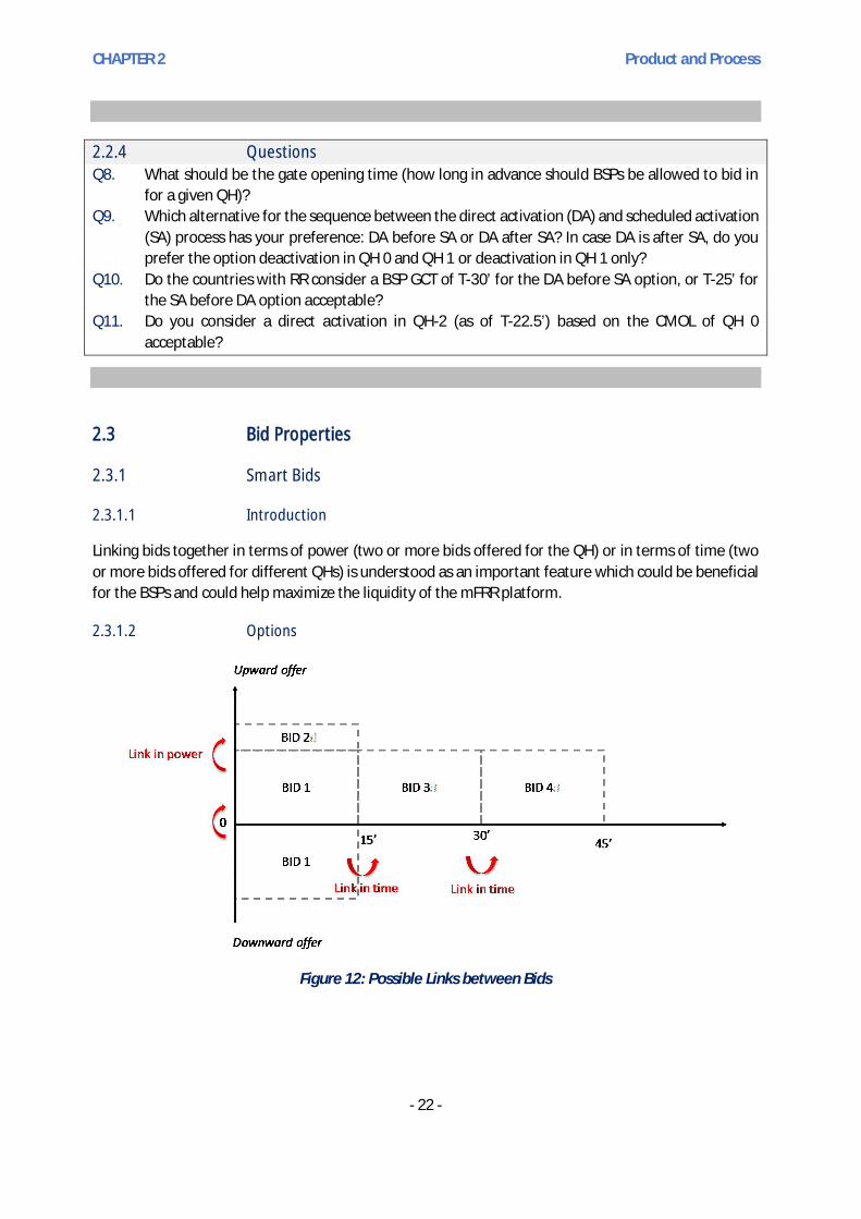
Linking bids together in terms of power (two or more bids offered for the QH) or in terms of time (twoor more bids offered for different QHs) is understood as an important feature which could be beneficialfor the BSPs and could help maximize the liquidity of the mFRR platform.
2.3.1.2 Options
Figure 12: Possible Links between Bids

CHAPTER 2 Product and Process
- 23 -
The following so-called ‘smart bids’ will be considered for inclusion in the MARI platform:
► Linked bid orders: the acceptance of a subsequent bid can be made dependent on the acceptanceof the preceding bids.
Example: BID 2 (child) can only be accepted if upward BID 1 (parent) is also accepted; i.e. theBID 2 (child) is linked to bid 1 (parent) and not vice-versa;
► Exclusive group orders: only one bid can be accepted from a list of mutually exclusive bids. Example:only one of the following bids can be accepted (they can differ in size, time, price and otherproperties): A1, A2, A3…An.
Example: An asset that is directly upward activated in one QH cannot necessarily be directlydownward activated in the same QH in order to ensure that the minimum delivery period oftheir asset is respected. In the figure above, this is illustrated by Bid 1 that is offered both forupward and downward activation, but that can only be activated once.
Smart bids could allow BSPs to offer more flexibility, maximize the opportunity to be activated by fittingwith TSO needs, reduce costs of balancing, reduce counter activations and contribute to an efficient andcompetitive balancing market. For example, by linking bids BSPs could reflect the start-up costs andpower limits of their units more correctly. In the drawing shown above this can be shown as follows: theprice of BID 1 is 70 €/MWh and includes a starting cost of 1000 € while the price of BID 2 is only 50€/MWh. There is no starting cost, only energy related costs but the use of this bid is conditional to thepreceding activation of BID 1.
However, smart bids generate complexity for the activation optimization function.
2.3.1.3 Analysis
Based on the draft ENTSO-E proposal for standard products and the analysis of sections 2.1 and 0, thefollowing starting points are assumed:
► Linking of bids between different platforms (e.g. PICASSO, TERRE projects) is a particular challenge.The need for this and alternatives for such links have to be addressed at a later stage ofdevelopment.
► Since the balancing needs of the TSOs are only known for the next QH, the clearing algorithm canonly optimize the selection of bids for this QH and not the subsequent ones, thus no links betweenbids in the next QH and bids in QHs thereafter are possible. For the clearing of the next QH, theactivation can only take into account the information of preceding QHs not of future QH.
► Other types of smart bids, next to linked bid orders and exclusive group orders, could be consideredwith respect to the impact they have on the time needed by the algorithm and the added value theygenerate (flexibility, lower costs,…).
2.3.1.3.1 Need for Technical Links between Bids in Different QHs
Due to the nature of the direct activation process and the timing of activations and gate closure timesthere is a need to ‘technically’ link bids between QHs. E.g. due to the fact that the results of the mFRR

CHAPTER 2 Product and Process
- 24 -
platform for QH 0 are known only after the BSP GCT for QH 1, a technical link between bids in QHs 0 and1 permits to avoid that the underlying asset of a bid is activated twice, i.e. with overlapping deliveryperiods but activated in different QHs. Such technical links between bids will be especially needed for aBSP with small portfolios or for countries with unit bidding.).
Several situations exist which require a technical linking between bids over different QHs, often relatedto the interaction between DA and SA:
► In alternatives 1 (see section 2.2.3.2), an asset that has been scheduled activated on QH 0 for itsmaximum power output cannot be direct activated on QH 1. The corresponding asset will actuallynot be able to provide the additional power output required to satisfy the DA need. The twoactivations do actually overlap;
► In alternatives 1 and 2 (see section 2.2.3.2), an asset that has been direct activated on QH 0 for itsmaximum power output cannot be direct activated on QH 1. The corresponding asset will actuallynot be able to provide the additional power output required to satisfy the second DA need. The twoactivations do actually overlap;
► For activations where the delivery period is between 5 and 20 min, this linking between bids willeven have to extend over more than one QH.
► Therefore the Activation optimization function (AOF) will need to be able to make the necessarylinks between bids in different consecutive QHs to avoid infeasible overlapping activations of thesame bid. Hence, BSPs will be required to indicate if bids in consecutive QHs are linked, i.e. toindicate if the underlying assets of a bid are the same as a bid offered in previous QH(s). An analysiswill be done in order to see if and how this feature will be implemented. This will make the wholeprocess more complicated as inputs from all activations (DA or SA) need to be given to the nextCMOL.
2.3.1.3.2 Possibility for Economical Optimisation based on Technical Links
Although technical links between bids arise from a technical need, they create new possibilities tooptimize activations and costs. By linking bids over QHs, the issue of start-up costs and not to pay themmore than once in several consecutive QHs can be tackled. A logic could be implemented toautomatically adapt the bid price of the same bid for the next consecutive QH based on informationgiven by the BSP when the bids were introduced. This means that the price of a bid for consecutiveactivations after the first activation could be lower, e.g. by the amount of the start-up cost.Consequently, it would increase the probability of the bid being selected again in the following activationperiod.
2.3.1.3.3 Conclusions
For the mFRR process, we propose allowing linking of bids, i.e. ‘smart bids’, by BSPs for economic reasonswithin the same QH, not between QHs. However, not all possible links should be allowed and thereshould be limits to the possibilities of linking (e.g. maximum number of linked bids). A methodology tolink bids over different QHs in order to avoid overlapping activation of the same bid in different QHs (i.e.linking for technical reasons) is required.

CHAPTER 2 Product and Process
- 25 -
2.3.1.4 Questions
Q12. Should there be a possibility to introduce ‚smart bids‘ and if so, which options to link bids shouldbe foreseen?
Q13. Are technical links between bids in different QHs necessary? If yes which should be implementedand why?
2.3.2 Divisibility of Bids
2.3.2.1 Introduction
Divisibility refers to a parameter of the bid specifying whether the bid can be partially activated or not.This section examines alternatives for having a cap on the bid size for indivisible bids and alternativerules for accepting and rejecting indivisible bids in the algorithm including the possibility to havetolerance bands for TSOs' needs.
2.3.2.2 Indivisible Bids - Maximal Size
2.3.2.2.1 Options
To carefully consider where to set the maximal size of the indivisible bids is important for the liquidityof the platform.
A small investigation among the majority of TSO participating in the project shows that most TSOs allowindivisible bids at least implicitly. Therefore indivisible bids should be allowed.
There is a great variance concerning the preferred maximum bid size which varies from 25 MW to 310MW.
2.3.2.2.2 Analysis
In the following Table 4, two options are compared. Option 1 is 25 MW which stands for a smallmaximum bid size and Option 2 is 310 MW which stands for a big maximum bid size. The concreteproposal for a maximum bid size can differ to these two options. Moreover, the comparison is based onthe assumption that the maximum bid size should be the same in the whole cooperation.

CHAPTER 2 Product and Process
- 26 -
Criteria Explanation 25 MW 310 MW
Liquidity The higher the maximum bid size, the higher theliquidity, because units which can only be switched onor off are not excluded from the market.
-1 1
Avoid marketabuse
The higher the maximum bid size, the higher thepossibility of market abuse especially in smallcountries with a high market concentration.
1 -1
Possibledeviations fromneed
The higher the maximum bid size, the higher thepossible deviations from the need.
1 -1
Changes tocurrent marketdesign
Both options require changes in the current marketdesign in at least some countries of the MARI project.
1 1
Implementationeffort
Both options will presumably have the sameimplementation effort.
1 1
Incentives forBSPs to beflexible
The smaller the maximum bid size, the higher theincentives for BSPs to become flexible.
1 -1
Distribution ofactivatedbalancingenergy
In the case of an unexpected outage of power unitproviding balancing energy, it is better to haveactivation distributed among more units with smalleractivated volumes.
1 0
Table 4: Comparison of the Two Options for a Maximum Bid Size of Indivisible Bids Representing aSmall (Option 1) and a Big (Option 2) Maximum Bid Size.
The comparison shows that the most important question is if promoting market liquidity is moreimportant than avoiding market abuse, reducing deviations from need and incentivizing BSPs to beflexible.
In that sense, a compromise could be to have a rather limited maximum indivisible bid size and to createspecific products to allow for a relatively low number of specific units with a higher size to still participatein the market.
2.3.2.2.3 Questions
Q14. If there should be a maximum size for indivisible bids, how large should the maximum be?
2.3.2.3 Divisible Bids – Minimum Activation and Granularity of Activation
The TSOs will investigate, together with the introduction of an indivisible bid, the possibility for BSPs todeclare part of the divisible bid as minimum power, i.e. the minimum power that has to be activated,otherwise the bid can't be activated at all.
CHAPTER 2 Product and Process
- 27 -
Example:
A divisible bid of 50 MW with a minimum quantity of 20 MW means that either at least 20 MW from thisbid are activated (up to 50 MW in a divisible manner), or no activation from this bid takes place. Anotherimportant feature to be analysed is the increment amount of activation for divisible bids (granularity ofactivation) that the algorithm can result in, for example can activation of the divisible bid be :[20 MW,20.01 MW, 20.02 MW] or [20 MW, 21 MW, 22 MW].
2.3.2.3.1 Implications of Existence of Divisible and Indivisible Bids
Two options concerning rejection of bids are to be thought of (see section 3.2.2.2 IV) as well as thefeature of the tolerance band for a TSO need which can mitigate the occurrence of such rejections (seesections 3.1.2.2 and 3.2.2.2 IV). Using a tolerance band by TSOs means that for a TSO more or less poweris activated compared to its actual need.
Certain criteria are listed which could be used to assess the two options described in CHAPTER 3 togetherwith the option to not allow indivisible bids. These are listed in the relevant section 3.2.2.2 IV, due tothe strong link to the algorithm.
2.3.2.3.2 Questions
Q15. Do you foresee using indivisible bids?
Q16. Do you need the possibility to declare minimum activation in divisible bids?
Q17. What should the granularity of activated volume be for divisible bids (e.g. 0.1 MW or 1 MW)?
2.3.3 Reliability of Bids
Reliability of bids can be understood in two possible ways:
A. Reliability of cross-border exchange: This describes the reliability of the cross-border exchangeif a bid in LFC block A has been activated for LFC block B. The reliability of the cross-borderexchange should be 100% irrespective of a possible outage of a power plant of the BSP in LFCblock A or other disturbances. When such a situation presents itself, the non-compliancy of theBSP will lead to an additional aFRR-demand or even results in an ACE in LFC block A (i.e.connecting TSO);
B. Reliability of bids: This describes the reliability of a bid. This can vary from BSP to BSP andespecially from country to country depending on the back-up requirements, unitbidding/portfolio bidding and the fact that real time change of schedules by market parties areallowed or forbidden. The requirements concerning reliability and the penalties in case of non-delivery shall be further discussed in the work stream harmonization of TSO-BSP rules.
Reliability of bids is not to be confused with the concept of firmness of bids. Firmness of bids refers tothe fact that as of a given point in time, e.g. GCT, both the volume and price of a submitted bid cannotbe changed anymore, i.e. the bid is firm. As of this point, the bid is expected to deliver once activatedaccording to the reliability requirements discussed above. In the public consultation of the Explore study,

CHAPTER 2 Product and Process
- 28 -
some respondents argued in favour of having non-firm bids, i.e. having the firmness deadline only at thepoint of activation. Because this would lead to additional complexity for the algorithm, system securityrisks and a shift in responsibility from BSP to TSO regarding reliability, the idea of non-firm bids isconsidered as non-optimal.
We propose requiring a 100% reliability of the cross-border exchange, but how to deal with non-compliancy and whether there are special challenges related to the physical firmness of HVDC cablesshall be further discussed in the work stream harmonization of TSO-BSP rules.
We propose that the deadline for bid firmness shall be the same as GCT for bid submission by BSPs.
2.3.4 Minimum Duration between the End of Deactivation Period and theFollowing Activation
Certain units may require some time in a rest state after the end of a deactivation period before theyare able to be activated again. The GLEB foresees in Article 25.5 that BSPs shall, as one of the variablecharacteristics of a standard product, determine the minimum duration between the end of thedeactivation period and the following activation.
The fact that the result of the clearing for QH 0 is known only after the BSP GCT for QH 1 necessitates aform of technical linking of bids between consecutive QHs to allow for this characteristic to be takeninto account by the algorithm as discussed in section 2.3.1.2. This way it can be avoided that the samebid is activated again too shortly after a deactivation.
2.3.4.1 Questions
Q18. Do you foresee using a "resting time", i.e. a minimum time between activations?
Q19. The granularity of bid volumes (divisble with 5 MW, 1 MW or 0.1 MW etc.) has not been discussedin this document. What would be a relevant granularity for expressing your bid volume?
2.4 Rules for Balancing Need
2.4.1 Restrictions on Activation Volume
2.4.1.1 Introduction
The question of how much each TSO can activate through the platform relates to the operationalsecurity. According to the GLSO (article 119 and 157), each LFC block shall jointly develop dimensioningrules for FRR, taking into account historical imbalances and dimensioning incidents of the LFC block. TheTSOs of a LFC block determine the geographical distributions for the FRR capacity and limitations onexchange and sharing within the LFC block. The TSOs of the LFC blocks that consist of the synchronousareas determine the geographical distributions for the FRR capacity and limitations on exchange andsharing within and between synchronous areas.

CHAPTER 2 Product and Process
- 29 -
Furthermore, because of potential agreements for sharing and exchange of mFRR balancing capacitywithin an LFC block or between LFC blocks, a TSO may have a larger balancing need than the bids madeavailable for the platform. This implies that the restriction on submitting balancing needs not exceedingthe volume of bids depends on these agreements between TSOs or LFC blocks. The TSOs of the LFC blockare responsible for the surveillance of whether TSOs' needs and bid volumes are in line with relevantagreements.
2.4.1.2 Options
In a non-emergency situation, it is proposed to have two restrictions on the volume of balancing needsrequested from the platform by a TSO:
1) The total volume of needs (DA and SA) requested by TSO A from the platform for a certaindirection (upward or downward regulation), as reported in GLEB Art. 29, must not exceed:
a. The volume from bids (DA and SA) submitted by the TSO A;
b. The volume from bids (DA and SA) submitted by another TSO B for the TSO A as a resultof a balancing capacity exchange between the TSOs;
c. The volume from bids (DA and SA) that corresponds to a sharing of reserves agreementbetween the TSO A and other TSOs, under the condition, that nobody from the otherTSOs has requested them already (mutually exclusive relation between the TSOs of thesharing agreement).
2) The total volume of DA needs requested by TSO A from the platform for a certain direction(upward or downward regulation), must not exceed:
a. The volume from DA bids submitted by the TSO A;
b. The volume from DA bids submitted by another TSO B for the TSO A as a result of abalancing capacity exchange between the TSOs;
c. The volume from DA bids that corresponds to a sharing of reserves agreement betweenthe TSO A and other TSOs, under the condition that nobody from the other TSOs hasrequested them already (mutually exclusive relation between the TSOs of the sharingagreement).
With the second restriction, if a TSO submits only SA bids to the platform, it is forbidden for the TSO touse DA bids. On the other hand, if a TSO or the TSOs of an LFC block submit only DA bids to the platform,the TSO is allowed to use up to the same volume of SA bids for two reasons:
- to increase liquidity of DA bids;
- DA bids are the bids that are always also scheduled activatable.
Example:
Below, examples are given to clarify the implications of the restrictions.The examples applies to onespecific activation direction. Either all bids are upward or downward.
For restrictions 1.a and 2.a:
► If a TSO A submits 200 MW of SA bids and 0 MW of DA bids, the TSO A is not allowed to use DAbids, but only SA bids up to 200 MW.

CHAPTER 2 Product and Process
- 30 -
► If a TSO A submits 100 MW of SA bids and 100 MW of DA bids, the TSO A is allowed to use up to100 MW of DA bids and 100 MW of SA bids or up to 200 MW of SA bids.
For restrictions considering the case of 1.b and 2.b:
► If a TSO A submits 200 MW of SA bids and 0 MW of DA bids, and another TSO B submits due toa Balancing Capacity exchange agreement 0 MW of SA bids and 150 MW of DA bids on behalfof TSO A:
• the TSO A is allowed to use up to 150 MW DA bids, and 200 MW SA bids
• or up to 350 MW only SA bids.
For restrictions considering the case of 1.c and 2.c:
► If a TSO A submits 200 MW of SA bids and 0 MW of DA bids, and it has an mFRR sharing ofreserves agreement with another TSO B of 0 MW of SA bids and 150 MW of DA bids:
• If TSO B has not yet requested the DA bids at all:
• the TSO A is allowed to use up to 150 MW DA bids, and 200 MW SA bids
• or up to 350 MW only SA bids.
• If TSO B has requested e.g 50 MW from the shared DA bids:
• the TSO A is allowed to use up to 100 MW DA bids, and 200 MW SA bids
• or up to 300 MW only SA bids.
2.4.1.3 Analysis
Can the MARI platform be used to facilitate interconnector controllability?
In certain situations TSOs need the facility to manage the operational flow range of HVDC links. In theTERRE cooperation this is facilitated within the optimization algorithm by allowing the TSO to submit aminimum and/or maximum exchange.
Example:
► TSO 1 and TSO 2 both have mFRR needs of 0 MW. The planned HVDC flow from TSO 1 > TSO 2is 30 MW for the target QH. TSO 1 requests a flow of <25MW for the target QH. This is consideredby the optimization algorithm which issues instructions of -5MW in TSO 1 and +5MW in TSO 2plus the new HVDC flow of 25MW. The energy balance in both TSO areas is unchanged but nowthe HVDC flow respects the limitation imposed by TSO 1.
In this example, we describe a simple scenario (no mFRR need) to illustrate the process. Settlement ofthese types of actions should adhere to the principle that the requesting TSO will be responsible for thecosts relating to bids accepted for the above purposes (in the previous example TSO 1 will be responsiblefor the costs relating to bids accepted to facilitate flow change on HVDC).
To calculate the appropriate settlement responsibilities in more complex scenarios, the MARI platformcan run two optimizations (either in parallel or sequentially):
► Constrained: As described above, HVDC limitations included;
CHAPTER 2 Product and Process
- 31 -
► Unconstrained: Ignoring HVDC control limitations (only considering mFRR needs) for computationof the marginal price.
2.4.2 Allowing Price Dependent Needs
A TSO can balance its area(s) with several balancing products. When the TSO has alternative measuresto manage an imbalance the ability to specify a limit on the price will remove uncertainties and allowthe TSO to utilize available resources cost efficiently. It may also lead to more needs submitted to theplatform, since it removes the incentive for the TSO not to submit needs due to the expectation ofalternative measures being less costly.
Options for price dependency:
► Inelastic: not priced (the volume is absolutely required by the TSO);
► Elastic: One or more request levels with volume and max/min price they are willing to accept for up-/down activation.
In the MARI Project, we will take the possibility of elastic demands into account in the design. On theother hand, we also need to take into account the selected option of timing and settlement, because forsome options the elastic demand may not be possible.
2.4.3 Questions
Q20. Do you have any comments on the Rules for Balancing need? If yes, elaborate.

CHAPTER 3 Specification of Activation Optimization Function
- 32 -
Specification of Activation Optimization Function
3.1 Inputs for the Merit Order List and Optimal Outputs
3.1.1 Introduction
The Activation Optimization Function (AOF) that will be used in MARI is based on the maximization ofthe social welfare.
A scheme of the optimization model is presented in Figure 13. As illustrated in this figure, theoptimization model uses as input the TSO demands, the BSP bids, as well as network information, i.e.,cross-zonal capacities (CZC) or any relevant network constraints and HVDC constraints. It creates a costcurve consisting of the TSO demands and the Common Merit Order List (CMOL) of all bids, and based onthis curve as well as on all defined constraints, it provides the optimal social welfare, the satisfieddemands, the accepted bids, the XB marginal prices and the XB commercial schedules.
Figure 13: Scheme of Activation Optimization Function
The following subsection presents the structure of the inputs and outputs of the AOF.

CHAPTER 3 Specification of Activation Optimization Function
- 33 -
3.1.2 Analysis
3.1.2.1 Structure of Bids
The submitted bids have the following features:
► Quantity [MW] (for the sake of the algorithm examples MWh is used in this chapter);
► Price of the bid (bid price)3 [€/MWh];
► Method of activation (SA or DA+SA);
► Divisibility (divisible or indivisible);
► Location (e.g., the country, LFC area or LFC block);
► Minimum duration between the end of a deactivation period and the following activation [min];
► From the algorithm point of view, it is important that prices of divisible linked bid orders are non-decreasing (monotonic objective function);
► Regarding smart bids, apart from the features stated above, there must be an indication (a flag orID) showing these bids belong to a set of linked bids.
Example:
Quantity [MW]: 10Price of the bid [€/MWh]: 30Divisibility (divisible or indivisible): divisibleLocation: Country A
Minimum duration between the end of a deactivation period and the following activation [min]:15
3.1.2.2 Structure of Demands
As described in section 2.4.2, TSO demands are assumed to be elastic (price dependent), as all principlesconsidered for elastic demands hold also for inelastic (price independent) demands.
TSO demands have the following features:
► Quantity [MW or MWh] (for the sake of the algorithm examples MWh is used in this chapter);
► TSO demand price [€/MWh]: this will provide flexibility to the TSOs to determine if their need willbe satisfied by MARI or by an alternative possibility, and will help them to deal with uncertainties. ATSO can also declare an inelastic need;
► Location of demand (e.g., the country, LFC area or LFC block);
► Purpose: balancing purposes or other purposes;
3 Please note that there must always be a bid price, which shall not be confused with the marginal price.

CHAPTER 3 Specification of Activation Optimization Function
- 34 -
► Tolerance band: it means that a TSO can declare a range in which additional or lower energy isactivated compared to its demand submitted to the platform. Note that TSOs will analyse thisfeature further.
► Please note that all demands are considered to be divisible. An example of a demand is provided inTable 5.
Regarding the sign convention used in this Chapter, we note that:
► For positive needs (short TSOs), a positive price indicates that a TSO is willing to pay (maximum) thisprice in order for its need to be satisfied. On the other hand, a negative price indicates that the TSOis willing to be paid (at least) with the submitted price in order for its needs to be satisfied.
► For negative needs (long TSOs), a positive price indicates that the TSO is willing to be paid (at least)with the submitted price in order for its needs to be satisfied. On the other hand, a negative priceindicates that the TSO is willing to pay (maximum) the submitted price in order for its need to besatisfied.
► For upward offers, a positive price indicates that the BSP wants to be paid (at least) with thesubmitted price in order to be activated. On the other hand, a negative price indicates that the BSPis willing to pay (maximum) the submitted price in order to be activated.
► For downward offers, a positive price indicates that the BSP is willing to pay (maximum) thesubmitted price in order to be activated. On the other hand, a negative price indicates that the BSPwants to be paid (at least) the submitted price in order to be activated.
TSO Demand Name Quantity(MWh)
TSO Demand Price(€/MWh)
Elastic/Inelastic
Location
TSO 1 Positive demand 1 100 10 Elastic Country ATSO 2 Positive demand 2 100 -- Inelastic LFC area XTSO 2 Negative demand
3-50 -20 Elastic LFC area XX
Table 5: Demand Structure
In Table 5, TSO 1 has an elastic positive demand of 100 MWh with a price of 10 €/MWh. This impliesthat this TSO is willing to pay a maximum of 10 €/MWh to satisfy its demand. TSO 2 has an inelasticpositive demand of 100 MW which is located in the internal zone X and an elastic negative demand of50 MWh located in the LFC area XX with a price of -20 €/MWh. That is, TSO 2 is willing that its demandof 100 MWh in the LFC area X will be met irrespective of (high or low) marginal prices, while he is willingto satisfy its demand of -50 MWh in the LFC area XX paying maximum 20 €/MWh.

CHAPTER 3 Specification of Activation Optimization Function
- 35 -
Figure 14: An Example of Cost Curve Formed by Bids and Elastic Demands
3.1.2.3 Example of the Cost Curve
A cost curve consists of a CMOL and the TSO demands. An example of such a curve is illustrated in Figure14 based on the information of offers and demands provided in Table 6.
TYPE Quantity (MWh) TSO Demand Price/OfferPrice (€/MWh)
Elasticity ofDemand
Negative demand (TSO 1) -100 -100 ElasticNegative demand (TSO 2) -100 -50 ElasticPositive demand (TSO 3) 250 65 ElasticDownward Offer (DO BSP1) 200 50 --Downward Offer (DO BSP2) 100 30 --Upward Offer (UO BSP3) 300 80 --
Table 6: Example - Cost Curve Formed by Offers/Bids and Elastic Demands
3.1.2.4 Other Inputs
Other inputs of the AOF include ATC limits, power flow limits related to internal zones (i.e., mFRR biddingzones) and HVDC loss factors.
3.1.2.5 Optimal Output
The optimal clearing algorithm outputs are as follows:
► Accepted bids per each area [MW] (for the sake of the algorithm examples, MWh is used in thischapter);

CHAPTER 3 Specification of Activation Optimization Function
- 36 -
► Satisfied demands per each TSO[MW] (for the sake of the algorithm examples, MWh is used in thischapter);
► XB Marginal Prices per each area [€/MWh];
► Optimal Social Welfare [€];
► Used CZ Capacity, including flows at each border. We note that further flows may be needed, andtherefore be calculated by the algorithm, for example the flow between LFCl areas.
3.1.3 Questions
Q21. Are all relevant inputs being addressed in the clearing algorithm design? If not, could you pleasestate the elements that you are missing?
Q22. Are all relevant outputs being addressed in the clearing algorithm design? If not, could you pleasestate the elements that you are missing?
3.2 Criteria of the Clearing Algorithm
3.2.1 Introduction
In this section, we elaborate on the criteria to be considered in the clearing algorithm. These criteriadefine the objective function to be optimized and constraints to be respected. We assume that theoptimization of scheduled bids and demands will be carried out within a single auction, and there willbe one independent auction per 15-minute period.
This implies that the algorithm considers a single time interval (a single QH interval) without connectionof this interval to other 15-min intervals. Therefore, it is concluded that bids as well as TSO demandscannot be linked over time intervals, as already explained in CHAPTER 2.
Example:
Bid 1 is 50 MW in time interval t1.
Bid 2 is 55 MW in time interval t2 and can be activated only if Bid 1 is activated in intervalt1.
Such Bids are not considered in the algorithm.
3.2.2 Analysis
3.2.2.1 Objective Function: Maximizing Social Welfare
The objective of the clearing algorithm is to maximize the social welfare. In the context of balancingmarkets, the social welfare is the total surplus of all TSOs obtained from satisfying their demands andthe total surplus of BSPs resulting from the activation of their associated offers, as illustrated in Figure

CHAPTER 3 Specification of Activation Optimization Function
- 37 -
15. The curve consisting of positive TSO demands and downward BSP offers constitutes the consumercurve (based on economic theory), and therefore indicates what price consumers (TSOs and BSPs) areprepared to pay for consuming mFRR balancing energy, based on their expectations of private costs andbenefits. On the other hand, the curve consisting of negative TSO demands and upward BSP offersconstitutes the producer curve (based on economic theory), and therefore shows the price they areprepared to receive for supplying mFRR balancing energy. Social welfare, also known as economicwelfare, is the total benefit available to society from an economic transaction, and therefore is made upof the red area in Figure 15 which is the consumer and the producer surplus.
For inelastic demand, the social welfare cannot be determined (in theory infinite value), as the demandmust be satisfied at any cost. For implementation purposes, a price will always be assigned, but forinelastic demands, this price will be higher than any MARI offer and will represent the technical limit4 ofthe MARI AOF.
Figure 15: Social Welfare
The following example illustrates how the AOF maximizes the social welfare of a region consisting of twoTSOs. The inputs of the example are presented in Table 7 and the outputs of the example are presentedin Table 8.

CHAPTER 3 Specification of Activation Optimization Function
- 38 -
TYPE Quantity(MWh)
TSO DemandPrice/Offer Price(€/MWh)
Divisibility ofOffers
Positive demand (TSO 1) +100 1000 --Positive demand (TSO 2) +100 1000 --Upward Offer (UO BSP1) 100 10 DivisibleUpward Offer (UO BSP2) 100 20 IndivisibleUpward Offer (UO BSP3) 200 5 Indivisible
Table 7: Inputs for Example - Activation of Bids with the Aim of Maximization of Social Welfare
Type Activated Quantity/Satisfied Demand (MWh)
Positive demand (TSO 1) +100Positive demand (TSO 2) +100Upward Offer (UO BSP1) 0Upward Offer (UO BSP2) 0Upward Offer (UO BSP3) 200Social Welfare (€) Marginal Price (€/MWh)100·1000 - 100·5 + 100·1000 - 100·5 + 200·5 - 200·5= 199’000
5
Table 8: Output for Example
3.2.2.2 Constraints
Constraints are the criteria and conditions that must be respected by the algorithm.
I. Power Balance Constraints
Principles:
I.A : In of the special situation that no demands are submitted (i.e. zero total demand),, there is noactivation (no simultaneous upward and downward activations).
I.B: Total activated bids satisfy the total demands of the TSOs.
I.C: In the power balance constraint, netting of the TSO demands inherently occurs. The netting ofthe TSO demands occurs as long as it results in a higher social welfare and it does respect other technicalconstraints, e.g. power flow constraints.
Power balance constraints enforce the total demand to be satisfied. In other words, the total activatedupward bids and satisfied negative demands must be equal to the total activated downward bids andsatisfied positive demands. This does not hold if a demand tolerance band will be used. In this case, thetolerance band has also to be included in these power balance constraints.
We illustrate the power balance constraints through an example in ANNEX 1 - Examples of AlgorithmConstraints.

CHAPTER 3 Specification of Activation Optimization Function
- 39 -
II. Power Flow Constraints
Principles:
II.A: Respecting ATC limits of the corresponding TSOs.
II.B: Respecting Internal Zones with Any Resolution
II.C: TSOs building a Cluster
The power flow constraints guarantee that the accepted offers respect the cross- zonal capacity limitscommunicated by the TSOs. Note that the algorithm does not specify what these limits shall be; ratherthe algorithm must respect these limits irrespective of what they are.
For the purpose of design phase 1, we consider ATC limits and internal zones, which could be the sameas bidding zones or zones with a smaller or a higher resolution5 (size) than bidding zones. The resolutionof zones may vary depending on the need of a TSO for congestion management. Although the resolutionof zones is not discussed here, the algorithm must respect any resolution required.
The TSOs requiring that their area is split up into internal zones must also provide offers and demandswith corresponding location information. That is, if a TSO needs to specify 3 zones, this TSO must specifyaccordingly the location (zone) of its offers and demands.
The algorithm also foresees that some TSOs have a need for representing their network with a numberof zones. The electrical model behind these zones (e.g., the number of interconnecting lines betweenthe zones, the number of zones, the cross- zonal capacity (thermal limits of lines), etc.) are inputs fromrespective TSOs to the algorithm.
The only important feature is that the TSO, which gives its zones as inputs to the algorithm, must alsoprovide correspondingly location information regarding its demands and its offers.
Another possible constraint is the need of some TSOs to represent their network model building a clustertogether with other TSOs. If bids were to be activated within this cluster, bids from a certain TSO wouldbe given priority over the other TSOs to a certain amount of MWs. System security/congestionmanagement are stated as the reason for this arrangement. The inputs to the algorithm include thecontrol zones involved, the priority TSO and the amount of MW to be activated from this TSO.
We illustrate the power flow constraints through example in an ANNEX 1 - Examples of AlgorithmConstraints.
5 The topic will be further investigated with a focus on the compliance with GLEB

CHAPTER 3 Specification of Activation Optimization Function
- 40 -
III. HVDC Constraints
Principles:
III.A: Max ramp between two mFRR clearing intervals express the maximum change of powerexchange between two clearings intervals. Max ramp is defined per each border that includes HVDCinterconnectors. These ramps will be considered by the TSOs before submitting the ATC values for theHVDC interconnectors to MARI.
III.B: Not allowed flow means the balancing power exchange interval that is not possible due to thetechnical minimum power of HVDC interconnectors. Also, in this constraint, the power flow of the HVDCline from the previous clearing is important.
HVDC constraints conceptually can be understood similar to ATC from the algorithm point of view. Thatis, there are limits on the power that could flow through HVDC lines. However, the losses in HVDC linesshall be considered.
In the following, we elaborate on HVDC losses as well as HVDC dynamic constraints.
HVDC Losses
As for any AC transmission line, the physical flow on an HVDC interconnector is subject to losses.TheHVDC losses are explicitly modelled in the Day-Ahead Market Coupling and in TERRE. Therefore, in orderto be consistent with the markets in other timeframes, HVDC losses will also be considered in a similarway by the MARI AOF. . Thus, assuming the running-time of the algorithm would not be heavily impactedby this feature, it is explained in ANNEX 1 - Examples of Algorithm Constraints how the algorithm cantake into account the losses on HVDC cables.
Because of these losses, for each settlement period, the energy volume sent from an exporting area Amay differ from the received energy in the importing area B. This will also have an impact on the prices,and hence there will be a price difference between these two areas.
HVDC-Dynamics Constraints
HVDC constraints will be considered by the TSOs before they submit their inputs to MARI, and hencethe capacity of the HVDC cables that will be submitted to the optimization will integrate theseconstraints.
IV. Constraints on Prices: Unforeseeably Rejected Bids (URB)
In the presence of indivisible and divisible bids, bids with an offered price smaller than the marginal pricecan be rejected if this leads to a higher social welfare. If these bids are divisible (indivisible), they arecalled unforeseen rejected divisible (indivisible) bids (URBs). This is called paradoxically rejected divisiblebids in the Market-Coupling Model.
We note that the possible application of the tolerance band can reduce the occurrence of URBs.However, it is not guaranteed that the issue will be solved and it has not been analysed what the impactof this application will be. TSOs will analyse the potential application of a tolerance band and the effectit has on the URBs.

CHAPTER 3 Specification of Activation Optimization Function
- 41 -
The inclusion of URB constraints in the algorithm is still an open point. In the following, we explain theunforeseeably rejected divisible bids by using a simple example presented in Table 9. Note that in thisexample, the UO BSP2 is an unforeseeably rejected divisible bid. We consider that the demands areinelastic, and hence we assign them a very high price that represents the technical limit (10’000 in thiscase).
Type Quantity(MWh)
TSO DemandPrice/Offer Price(€/MWh)
Elasticity of Demand Divisibility ofOffers
Positive demand(TSO 1)
+100 100006 Inelastic --
Positive demand(TSO 2)
+100 10000 Inelastic --
Upward Offer (UOBSP1)
+190 10 -- Indivisible
Upward Offer (UOBSP2)
+8 20 -- Divisible
Upward Offer (UOBSP3)
+10 21 -- Indivisible
Upward Offer (UOBSP4)
+2 30 -- Indivisible
Table 9: Inputs for Example 10 - Unforeseen Rejected Divisible Bids
As shown in Table 10, the outcome of the algorithm, in terms of activated offers, balancing cost, andmarginal prices, is totally different with and without this constraint about unforeseeably rejecteddivisible bids.
Under the solution of allowing URBs, UO BSP2 is rejected. However, its offer price is smaller than itsmarginal price (20 €/MWh < 21 €/MWh). With this solution a higher social welfare is obtained than thatof avoiding URBs.
6 For the shake of the example the technical limit assumed for the inelastic TSO demand is 10000 €/MWh

CHAPTER 3 Specification of Activation Optimization Function
- 42 -
Type Output of Balancing CostMinimization (AllowingUnforeseen Rejected DivisibleBids)Activated Quantity/SatisfiedDemand (MWh)
Output of Market-Coupling model(Avoiding Unforeseen RejectedDivisible Bids)Activated Quantity/SatisfiedDemand (MWh)
Positive demand (TSO 1) +100 +100Positive demand (TSO 2) +100 +100Upward Offer (UO BSP1) +190 +190Upward Offer (UO BSP2) 0 +8Upward Offer (UO BSP3) +10 0Upward Offer (UO BSP4) 0 +2Marginal Price (€/MWh) €21/MWh €30/MWhSocial welfare (€) 100·10000 + 100·10000 -
100·21 - 100·21 + 190·21 +10·21 - 190·10 - 10·21 =1’997’890
100*10000 + 100*10000 – 100*30– 100*30190·30 + 8·30 + 2·30 -190·10 - 8·20 - 2·30 = 1’997’880
Table 10: Output for Example 10
Table 11 lists three criteria solely from the algorithm point of view and provides a qualitative evaluation.From a computation point of view, it needs to be investigated if the algorithm with the constraints ofavoiding unforeseably rejected divisible bids can find a solution within an acceptable time (around 1min).
We should also note that the complexity problem is a relevant criterion: the more complex the algorithmis, the harder to find an optimal outcome it is and the more time the algorithm will require. This mayhave an impact on the gate closure time.
To have a quantitative estimate of the impact of this constraint (e.g. computation time, balancing costs,the frequency of occurrence etc.), a precise simulation with a strong computation engine is required.

CHAPTER 3 Specification of Activation Optimization Function
- 43 -
Criteria Allowing UnforeseeablyRejected Divisible Bids(Social-Welfare Maximization)
Avoiding Unforeseeably RejectedDivisible Bids(Market-Coupling Algorithm)
Optimal Social Welfare Higher social welfare Lower social welfareComplexity Level ofAlgorithm
Low (Simple)(solving a primal clearingmodel)
High (Complex)(including a non-linear constraint andsolving a primal-dual problem)
Computation Time Lower computation time Higher computation time
Bid structure No particular incentive Incentivize (a) divisible bids and (b)indivisible bids of lower volume
Table 11: Criteria for Qualitative Evaluation of Allowing/Avoiding Unforeseen Rejected Divisible Bidsfrom the Algorithm Point of View
Further possible criteria are listed which could be used to assess the two options together with theoption to not allow indivisible bids:
► Complexity algorithm: Not allowing indivisible bids would reduce complexity drastically. AllowingUnforeseeably Rejected Divisible Bids is considered to have the least complexity.
► Incentives to offer divisible bids: In the case of Allowing Unforeseeably Rejected Divisible Bids, theincentives to offer divisible bids are higher compared to not allowing at all indivisible bids, butslightly lower in comparison to Avoiding Unforeseeably Rejected Divisible Bids.
► Transparency The results of the optimization are easier to check if indivisible bids are not allowed.
► Social welfare: Not allowing indivisible bids will reduce social welfare since liquidity is reduced.Allowing Unforeseeably Rejected Divisible Bids will be slightly better concerning social welfare thanAvoiding Unforeseeably Rejected Divisible Bids since a cheaper indivisible bid might be activatedinstead of a more expensive divisible bid;
► Consistency with other markets: For Day-Ahead market coupling, Avoiding Unforeseeably RejectedDivisible Bids is used and the recent results from the public consultation of the FCR cooperation alsoshowed a preference for Avoiding Unforeseeably Rejected Divisible Bids, (however, the latter is amarket for balancing capacity and not for balancing energy). In North American energy markets, theoption of Allowing Unforeseeably Rejected Divisible Bids is used.
V. Constraints on Prices: Unforeseeably Accepted Bids
The existence of complex bids, e.g. indivisible bids, in the MARI AOF introduces non-convexities in themathematical formulation of the optimization problem. Due to the non-convex nature of the problem,there may be cases where the resulting marginal price is lower (resp. higher) than the price of someupward (resp. downward) accepted bids. These bids incur financial losses for the BSPs and are calledUnforeseeably Accepted Bids (UAB). In the Day-Ahead Market Coupling, the same bids are referred toas Paradoxically Accepted Bids.
An example where an indivisible bid is unforeseeably accepted is presented below. The input data arepresented in Table 12.

CHAPTER 3 Specification of Activation Optimization Function
- 44 -
Type Area Volume (MWh) Price (€/MWh)Positive demand (long TSO) TSO 1 +100 InelasticUpward divisible bid 1 TSO 1 +50 10Upward divisible bid 2 TSO 1 +40 20Upward indivisible bid 3 TSO 1 +40 30Upward divisible bid 4 TSO 1 +100 60
Table 12: UAB Example: Input Data
The merit order list is presented in Figure 16.
Figure 16: UAB Example: Merit Order List
If the algorithm maximizes purely the social welfare with no further constraints, then the upwarddivisible bid 1 and the upward block bid 3 is fully accepted and only 10 MWh of the divisible bid 2 isaccepted. The resulting marginal price is set to 20 €/MWh. In this case, there are no unforeseeablyrejected bids, but the upward indivisible bid 3 is unforeseeably accepted as the bid price is 30 €/MWhand the resulting marginal price 20 €/MWh.
This can be avoided either by setting the price to 30 €/MWh (in this case, part of the upward divisiblebid 2 is unforeseeably rejected) or by rejecting the upward indivisible bid 3 and accepting the wholeupward divisible bid 2 and 10 MWh of the upward divisible bid 4 (in this case, the upward block bid 3 isunforeseeably rejected).
The final solution given by the AOF will not contain any UABs, i.e. one of the aforementioned optionswill be chosen, as this would require an extra payment of uplifts to the market participants in order forthem to recover their costs, and would hence deviate from the concept of marginal pricing. This will beachieved by a primal/dual formulation of the optimization – clearing and pricing in a single problem -with extra constraints to ensure that all BSPs recover their costs.
The unforeseeable acceptance and rejection rules are not relevant for elastic needs. As a consequence,the price in a given area may exceed for example the price of the elastic positive imbalance need in thearea.

CHAPTER 3 Specification of Activation Optimization Function
- 45 -
VI. Constraints on Activation Volumes: Scheduled Counter-Activations
With the term scheduled counter-activations, we refer to the simultaneous activation of a scheduledupward and a scheduled downward offer by the AOF in order to increase the social welfare. Due to thefact that all positive and negative demands, as well as all upward and downward bids are treated in asingle common merit order list, scheduled counter-activations could occur if some downward offers hadhigher prices than some upward offers, i.e. if some BSPs would be willing to pay higher prices to reducetheir production than the prices that some other BSPs would be willing to receive to increase theirproduction.
Figure 17 presents a merit order list. If a downward offer had a higher price than an upward offer thenthese two offers would be simultaneously activated, as this would result in a higher social welfare.
Figure 17: Merit Order List
An example is provided below. We consider a system of three TSOs. The volume of demands with limitprices and bid prices are presented in Table 13, and the ATC values are high enough not to affect thesolution.
Type Area Volume(MWh)
Price (€/MWh)
Negative demand (long TSO) TSO 1 100 -100Negative demand (long TSO) TSO 2 -100 -50Positive demand (short TSO) TSO 3 +150 100Downward bid (BSP 1) TSO 1 300 50Downward bid (BSP 2) TSO 2 100 30Upward bid (BSP 3) TSO 3 +300 40
Table 13: Example Input Data

CHAPTER 3 Specification of Activation Optimization Function
- 46 -
Figure 18 presents the merit order created for this example, and Figure 19 depicts the final activationsand flows.
Figure 18: Example Merit Order List
Figure 19: Example Activations
We observe that in this case upward and downward bids are simultaneously activated. More specifically,a 300 MWh downward bid is activated from BSP 1, 250 MWh from an upward bid is activated from BSP3, and the demands are fully satisfied. It is activated 100 MWh downward and 100 MWh upward beyondthe demands. The marginal price for this case is 40 €/MWh and the social welfare is 35 000 €.
Restricting the scheduled counter-activations would lead to the results presented in Figure 20 and Figure21.

CHAPTER 3 Specification of Activation Optimization Function
- 47 -
Figure 20: Scheduled Counter-Activations’ Restriction: Impact on Merit Order List
Figure 21: Scheduled Counter-Activations’ Restriction: Impact on Activations
In this case, only a 50 MWh downward offer from BSP 1 is activated, whereas the demands are fullysatisfied. Therefore, with this option we manage to limit the activation of offers. However, in this casethere is price indeterminacy (see further 4.3.4.5). The social welfare in this case is 32 500 €, and istherefore decreased by 2 500 €.
Note that scheduled counter-activations could be restricted, as presented in the previous example, byusing additional constraints in the AOF. This would, however, increase the complexity and could resultin higher computation times.

CHAPTER 3 Specification of Activation Optimization Function
- 48 -
In this particular example, the scheduled counter-activations could be avoided by introducing a pre-netting stage. After the pre-netting stage, only 50 MWh of the negative need of the TSO 2 would remainand the market clearing algorithm could run only with downward offers. However, when there is notenough ATC, a pre-netting stage is not sufficient to avoid scheduled counter-activations. We illustratethis by using the same example with the following ATC values, which are assumed to be symmetricalregarding the exchange direction:
Link ATC (MWh)TSO 1 – TSO 2 100TSO 1 – TSO 3 50TSO 2 – TSO 3 50
Table 14: Example Input ATC
With these ATC limitations, the 150 MWh upward need from TSO 3 can no longer be entirely nettedwith the other TSO needs. Since only 50 MWh can go through the ATC network between TSO 3 and eachother TSO respective area, only 100 MWh from TSO 3’s need can be satisfied through the pre-nettingprocess. Afterwards, both TSO 1 and TSO 3 will face a remaining need that could not have been netted,as illustrated in Figure 22.
Figure 22: Impact of a Congestion on Counter-Activations
TSO 1 will have a remaining 100 MWh downward need, and TSO 3 will have a remaining 50 MWh upwardneed. For them to be satisfied, a counter-activation has to occur: since both the links TSO 1 – TSO 3 andTSO 2 – TSO 3 are congested, the only solution is to activate an upward offer from BSP 3 and somedownward offer from BSP 1 or BSP 2. If we block this counter-activation, two needs could remainunsatisfied, even if they were submitted at any price (inelastic), which is not acceptable. This proves thata pre-netting process is not sufficient to address the problem of counter-activation prohibition.
It is also important to stress that a potential restriction of scheduled counter-activations could distortthe price signals in unpredicted ways, as presented in Figure 23 and Figure 24.

CHAPTER 3 Specification of Activation Optimization Function
- 49 -
Figure 23: A Restriction of Scheduled Counter-Activation Increases the Marginal Price
Figure 24: A Restriction of Scheduled Counter-Activation Decreases the Marginal Price
Table 15 provides the qualitative evaluation criteria for allowing or restricting the scheduled counter-activations.
CriteriaAllowing scheduled counter-activations
Restricting scheduledcounter-activations
Optimal Social Welfare Maximum social welfare Reduced social welfareComplexity Level of Algorithm Low (Simple) High (Complex)Computation Time Lower computation time Higher computation timeLiquidity Increased (more opportunities
for BSPs to be activated)No influence
Use of XB capacity Potential use of more XBcapacity (in one direction)
Limited use of XB capacity
Impact on other markets No influence No influenceAvailability of resources Reducing availability of
resourcesIncreasing availability ofresources
Activation serving balancingpurpose
Partially Yes
Table 15. Evaluation Criteria for Allowing or Restricting Counter-Activations
Regarding the criterion ‘Impact on other markets’, e.g. the Intraday (ID) Market, we consider that apotential allowance of scheduled counter-activations would not have any impact. More specifically, theGLEB includes several references aimed at guaranteeing that the balancing markets do not endangerthe efficiency of the previous markets such as the ID. Examples of such rules are the GCT, rules forupdating the positions from the BRPs, rules for the submission of balancing bids to the Europeanplatforms, as well as pricing and settlement principles. These references will be followed by MARI inorder to contribute to the efficient functioning of the energy markets (DA/ID). Moreover, the bidssubmitted to MARI shall be prequalified to fit the characteristics of the mFRR balancing product; thisclearly differentiates them from the authorized bids of the ID market. Therefore, due to the

CHAPTER 3 Specification of Activation Optimization Function
- 50 -
aforementioned features, the allowance, and also not allowance, of scheduled counter-activations inMARI shall not affect the liquidity of the energy markets.
A quantitative study would be necessary in order to identify the exact impact of scheduled counter-activations on the social welfare, computation times, marginal prices and use of XB capacity.
3.2.3 Questions
Q23. Do you agree with the maximization of social welfare as the main objective of the ActivationOptimization Function?
Q24. Do you prefer to allow or to block the scheduled counter-activations?
Q25. What are your views regarding unforeseeably rejected and accepted bids?
Q26. Which of the two options would you prefer regarding the handling of HVDC constraints?
3.3 Further Issues Connected to the Algorithm
3.3.1 Computation Time
The computation time of the algorithm is important as it has an impact on the gate closure time of MARI.For quantitative statements, a precise simulation with a strong computation engine is required.
3.3.2 Multiple Optimal Solutions
This section describes the cases where multiple optimal solutions exist, and proposes possible solutionsto choose a solution among these equally optimal solutions. We should remind that all these optimalsolutions result in the same optimal social welfare (same minimum balancing cost) and meet all theconstraints, described above.
3.3.2.1 Analysis
3.3.2.1.1 Case 1: A Set of Optimal Solutions with Different Marginal Prices
If a set of optimal solutions from the algorithm exists, but which lead to different marginal prices(optimal variables of the dual problem), two possible solutions are:
Solution case 1.A: The optimal solution leading to a smaller marginal price should be considered.
Solution case 2.B: The optimal solution respecting the increasing/decreasing order of offered pricesshould be considered.
Please note that since rejecting an unforeseen indivisible bid is allowed, both solutions result anyway toreject an unforeseen indivisible bid.
In the following example, the final solution is Solution A, as this solution results in a smaller marginalprice than that of solution B.

CHAPTER 3 Specification of Activation Optimization Function
- 51 -
Type Quantity(MWh)
TSO DemandPrice/Offer Price(€/MWh)
Divisibility ofOffers
Demand (TSO 1) +100 1000 --Demand (TSO 2) +100 1000 --Upward Offer (UO BSP1) +190 10 DivisibleUpward Offer (UO BSP2) +8 20 IndivisibleUpward Offer (UO BSP3) +10 21 IndivisibleUpward Offer (UO BSP4) +2 25 Indivisible
Table 16: Inputs for Example
Type Solution AActivatedQuantity/SatisfiedDemand (MWh)
Solution BActivated Quantity/SatisfiedDemand (MWh)
Demand (TSO 1) +100 +100Demand (TSO 2) +100 +100Upward Offer (UO BSP1) +190 +190Upward Offer (UO BSP2) 0 +8Upward Offer (UO BSP3) +10 0Upward Offer (UO BSP4) 0 +2Marginal Price (€/MWh) €21/MWh €25/MWhSocial welfare (€) 100·1000 + 100·1000 -
100·21 - 100·21 + 190·21 -190·10 + 10·21 - 10·21 =197’890
100·1000 + 100·1000 - 100·25 -100·25 + 190·25 - 190·10 + 8·25 -8·20 + 2·25 - 2·25= 197’890
Table 17: Output for Example
3.3.2.1.2 Case 2: A Set of Optimal Solutions with the Same Marginal Prices
If a set of optimal solutions with equal marginal prices (optimal variables of the dual problem of the dualalgorithm) exists, the solution leading to a smaller energy exchange (power flow) between TSOconnections is considered.
In the following example, the final solution is solution B, as this solution results in acceptance of UOBSP2 which is located in Area 2 as demand of TSO 2. However, solution A results in unnecessary flowfrom Area 3 to Area 2.

CHAPTER 3 Specification of Activation Optimization Function
- 52 -
Type Quantity(MWh)
TSO DemandPrice/OfferPrice (€/MWh)
Divisibilityof Offers
Area
Demand (TSO 1) +100 1000 -- Area 1Demand (TSO 2) +100 1000 -- Area 2Upward Offer (UO BSP1) +190 10 Divisible Area 1Upward Offer (UO BSP2) +8 20 Indivisible Area 2Upward Offer (UO BSP3) +10 20 Indivisible Area 3Upward Offer (UO BSP4) +2 20 Indivisible Area 4
Table 18: Inputs for Example
Type Solution AActivated Quantity/SatisfiedDemand (MWh)
Solution BActivated Quantity/SatisfiedDemand (MWh)
Demand (TSO 1) +100 +100Demand (TSO 2) +100 +100Upward Offer (UO BSP1) +190 +190Upward Offer (UO BSP2) 0 +8Upward Offer (UO BSP3) +10 0Upward Offer (UO BSP4) 0 +2Marginal Price (€/MWh) €20/MWh €20/MWhSocial welfare (€) 100·1000 + 100·1000 -
100·20 - 100·20 + 190·20 -190·10 + 10·20 - 10·20 =197’900
100·1000 + 100·1000 - 100·20 -100·20 + 190·20 - 190·10 + 8·20 -8·20+ 2·20 - 2·20 = 197’900
Table 19: Output for Example
3.3.3 Questions
Q27. If a set of optimal solutions exists, which lead however to different marginal prices, which of thetwo proposed approaches, Solution case 1.A or Solution case 2.B would you prefer?
Q28. Do you agree with the suggested approach when a set of optimal solutions with equal marginalprices exists?

CHAPTER 4 Settlement
- 53 -
Settlement
4.1 Introduction
This chapter explains the idea of Cross-border Marginal Pricing and options for how to handle TSO-TSOsettlement including the sharing of congestion rents. Since there is a link to TSO-BSP and TSO-BRPsettlement, and since the GLEB requires a framework for harmonization of terms and conditions for BSPsand BRPs (acc. to GLEB Art. 20), these topics are touched on in CHAPTER 6; however, only ideas on howthese topics could be approached are provided in this document.
4.2 Settlement Model and Fundamental Considerations
4.2.1 Cross-Border Marginal Pricing
Article 30 of EBGL provides guiding principles for the pricing of balancing energy. The pricing methodshall notably:
► be based on marginal pricing (pay-as-cleared);
► give correct price signals and incentives to market participants;
► take into account the pricing method in the day-ahead and intraday timeframes.
The MARI project proposes to use a cross border marginal price for the TSO-TSO and TSO-BSPsettlement. The cross border marginal price is the price of the last bid of the mFRR standard productwhich has been activated to cover the energy need for balancing purposes within an uncongested area.Therefore, it defines the value where the selling curve and the buying curve meet (e.g. 65 €/MWh inFigure 25).

CHAPTER 4 Settlement
- 54 -
Figure 25: Cost Curve Formed by Offers and Elastic Demands
Differences in prices occur in congested situations which are described in the following chapters.
The cross-border marginal price has the following advantages:
► As it is a marginal price, it is compliant with the GLEB requirements;
► XBMP contributes to establish a level playing field within the cooperation. BSPs providing the sameservice in an uncongested area are remunerated with the same price;
► As it is a marginal price, it does not incentivize BSPs to add a premium to the bid price (which canthen be cost-reflective);
► Cross-Border Marginal Pricing is currently used for market coupling and thus ensures consistencywith the pricing method in the day-ahead and intraday timeframes;
► A congestion rent appears in cases of congestion.
4.2.2 Case without Congestion
If no congestion applies within the cooperation, the highest activated bid price defines the TSO-TSOprice of the TSO-TSO-settlement as well as the TSO-BSP price of the TSO-BSP-settlement. Every BSPreceives the same price for activated balancing energy from the connecting TSO and every TSOpays/receives the same marginal price for imported/exported balancing energy.7
The following Figure 26 shows a qualitative example with two TSOs, TSO A and TSO B. In this simpleexample, it is assumed that all bids have the same volume. The demand of A (dA) and the demand of B(dB) is commonly activated (dAB) from a CMOL. In Figure 26 on the left side, the local demands and bidcurves are shown as well as the local marginal price (MPA and MPB) which would occur withoutcooperation. On the right side, the CMOL and the resulting cross-border marginal price (MPAB) is drawn.
7 Due to the presence of indivisible bids, there may be special cases when this does not always hold.

CHAPTER 4 Settlement
- 55 -
Figure 26: Local vs. Common Merit Order List, without Congestion
Figure 27: Settlement without Congestion
All BSPs receive the same (cross-border) marginal price (MPAB) from the connecting TSO from the TSO-BSP settlement (see Figure 27).
In this example, the TSO with the higher demand (TSO A) pays to BSP for one bid (A1) and the exportingTSO B pays to BSPs for four bids at the same marginal price.
Because TSO B pays to BSPs for the volume requested by TSO A, a TSO-TSO-settlement is needed tocompensate the exporting TSO B for the additional activation costs. If cross-border marginal pricing isapplied for TSO-TSO settlement, all TSOs take a proportional cost share according to their respectivedemand.
The cost differences caused by import or export are paid through the TSO-TSO settlement with the cross-border marginal price (MPAB).

CHAPTER 4 Settlement
- 56 -
For a better understanding, please find below a quantitative example:
Indicator TSO A TSO BRequested activation (demand) in MWh 90 10Activation in MWh 30 70Balancing energy export in MWh 0 60Balancing energy import in MWh 60 0Highest activated bid price in €/MWh 50 25
Table 20: Theoretical Example without Congestion
Because there is no congestion, the cross-border marginal price is 50 €/MWh (max of all activated bids).TSO B exports 60 MWh (70 MWh-10 MWh) and TSO A imports 60 MWh (90 MWh-30 MWh). For TSO-TSO settlement TSO A pays 50 €/MWh for 60 MWh imported balancing energy. At the end each TSO haspaid the costs for its requested activation (local demand x marginal price).
The following financial flows occur. For simplicity reasons, it is assumed that the imbalance price is basedon the marginal price and mFRR is the only product activated and therefore BRPs pay the cross-bordermarginal price.
Step Evaluation TSO A TSO B
1 Requested activation (demand) in MWh 90 102 Activation in MWh 30 703 Highest activated bid price in €/MWh 504 Costs of local activation (TSO-BSP Settlement) (2)x(3) in € 1500 35005 Costs of local demand (TSO-BRP Settlement) (1)x(3) in € 4500 5006 TSO-TSO settlement (Import (“+”); Export (“-“)) in € [(1)-(2)]x(3)=(5)-(4) 3000 -30007 Financial flows (4)+(6)-(5) 0 0
Table 21: Financial Flows without Congestion 8
This settlement method guarantees the financial neutrality of TSOs (acc. to line 7 of Table 21) if the costsof local demand are recovered by the TSO-BRP settlement.
4.2.3 Case with Congestion
A congestion originates in the situation where cross- zonal capacity available between locations is notsufficient to accommodate all economically optimal cross-border exchanges, according to previouslyestablished criteria (i.e. optimization of social welfare).
The common platform for mFRR will facilitate the netting of TSO mFRR needs and optimize the allocationof cross zonal capacities. Thus, congestion situations are to be likely in the context of MARI activations.
After optimization, for economic reasons, the energy flows from the cheapest to the more expensivearea. In cases of congestion, there is a price difference between the price that an area is “willing to pay”and the price that the other area is “willing to receive” at either side of the interconnector. Thus, asurplus from the congested interconnection will occur.
8 The convention for costs (positive) and proceeds (negative) is consistent with Art. 46 of the GLEB.

CHAPTER 4 Settlement
- 57 -
Congestion rent for activation of mFRR energy can be stated as follows:
Congestion rent [€] = Imported volume [MWh] x (MP of the exporting TSO [€/MWh] – MP of theimporting TSO [€/MWh])
Example:
In Figure 28 it is assumed that bid B4 is not available due to a congestion.
Figure 28: Local vs. Common Merit Order List, with Congestion
TSO A needs to activate a second local bid (A2) which is more expensive than the unavailable bid B4. Asa result, there are two marginal prices at each side of the border (MPA and MPB).
The TSO-BSP price at control block A is MPA and the TSO-BSP price at control block B is MPB, BSPs aresettled at different prices according to their connecting TSO.
In the example in Figure 29, the TSO with the higher demand (TSO A) pays to BSPs for 2 bids and theexporting TSO B pays to BSPs for 3 bids.
TSO A caused one and a half bids of the activation of TSO B. The price could be MPA or MPB.
Figure 29: Settlement with Congestion
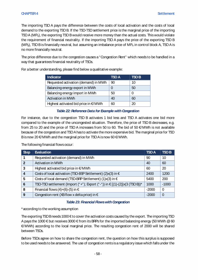
CHAPTER 4 Settlement
- 58 -
The importing TSO A pays the difference between the costs of local activation and the costs of localdemand to the exporting TSO B. If the TSO-TSO settlement price is the marginal price of the importingTSO A (MPA), the exporting TSO B would receive more money than the actual costs. This would violatethe requirement of financial neutrality. If the importing TSO A pays the price of the exporting TSO B(MPB), TSO B is financially neutral, but assuming an imbalance price of MPA in control block A, TSO A isno more financially neutral.
The price difference due to the congestion causes a “Congestion Rent” which needs to be handled in away that guarantees financial neutrality of TSOs.
For a better understanding, please find below a qualitative example:
Indicator TSO A TSO BRequested activation (demand) in MWh 90 10Balancing energy export in MWh 0 50Balancing energy import in MWh 50 0Activation in MWh 40 60Highest activated bid price in €/MWh 60 20
Table 22: Reference Data for Example with Congestion
For instance, due to the congestion TSO B activates 1 bid less and TSO A activates one bid morecompared to the example of the uncongested situation. Therefore, the price of TSO B decreases, e.g.from 25 to 20 and the price of TSO A increases from 50 to 60. The bid of 50 €/MWh is not availablebecause of the congestion and TSO A has to activate the more expensive bid. The marginal price for TSOB is now 20 €/MWh and the marginal price for TSO A is now 60 €/MWh.
The following financial flows occur:
Step Evaluation TSO A TSO B1 Requested activation (demand) in MWh 90 102 Activation in MWh 40 603 Highest activated bid price in €/MWh 60 204 Costs of local activation (TSO-BSP Settlement) (2)x(3) in € 2400 12005 Costs of local demand (TSO-BRP Settlement) (1)x(3) in € 5400 2006 TSO-TSO settlement (Import (“+”); Export (“-“)) in € [(1)-(2)]x(3 (TSO B))* 1000 -10008 Financial flows (4)+(6)-(5) in € -2000 09 Congestion rent (XB flow x delta price) in € -2000 0
Table 23: Financial Flows with Congestion
*according to the working assumption
The exporting TSO B needs 1000 € to cover the activation costs caused by the export. The importing TSOA pays the 1000 € but receives 3000 € from its BRPs for the imported balancing energy (50 MWh @ 60€/MWh) according to the local marginal price. The resulting congestion rent of 2000 will be sharedbetween TSOs.
Before TSOs agree on how to share the congestion rent, the question on how this surplus is supposedto be used needs to be answered. The use of congestion rents is a regulatory issue which falls under the

CHAPTER 4 Settlement
- 59 -
scope of the Member States and NRAs. The TSOs will cooperate with the NRAs in any related aspect thatwould be required regarding this issue.
In the context of the MARI project, it has been agreed as a working assumption at this stage that, thecongestion rent resulting from mFRR activations will be considered a congestion income, assumed asthe result of an implicit allocation of available capacity in the context of balancing services.
This interpretation would be the same as that used in other timeframes such as the day ahead market(Multi Regional Coupling) and the current approach of the project TERRE (RR). Taking the previousassumption into account, the aspects related to the use of congestion rents would fall under the existingregulations on this topic (Regulation 714/2009 article 16-6), and the possible future treatment underthe proposal of Clean Energy for All Europeans:
“Any revenues resulting from the allocation of interconnection shall be used for […] (b) Maintaining orincreasing interconnection capacities through network investments, in particular in newinterconnectors.[…]”
NRAs will be consulted on whether this assumption, i.e the applicability of Regulation 714/2009 article16-6 is valid or not.
4.2.4 Effects of XB-Marginal Pricing on Imbalance Pricing and Local Imbalance
This section illustrates some expected implications of the cross-border marginal price on the imbalanceprices. The considerations here are not necessarily shared by all TSOs and are mainly put forward byTSOs allowing the BRPs to move in real time (applying a so-called reactive balancing philosophy).
4.2.4.1 Imbalance Price and Local Imbalance Stipulations of the GLEB
The imbalance price serves as a financial incentive for BRPs to be balanced or to support the system tobe balanced. Therefore, the GLEB imposes several requirements that links balancing energy pricing withimbalance pricing and sets directions which should be ensured via the settlement:
► Whereas 14 – The pricing method for standard products for balancing energy should create positiveincentives for market participants in keeping and/or helping to restore the system balance of theirimbalance price area, reduce system imbalances and costs for society[…];
► Whereas 17 - The general objective of an imbalance settlement is to ensure that balance responsibleparties support the system's balance in an efficient way and to incentivise market participants inkeeping and/or helping to restore the system balance[…];
► Article 309(1)(d) - give correct price signals and incentives to market participants;
► Article 4410(1)(a) - establish adequate economic signals which reflect the imbalance situation;
9 Pricing for balancing energy and cross-zonal capacity used for exchange of balancing energy or for operating theimbalance netting process.
10 General settlement principles

CHAPTER 4 Settlement
- 60 -
► Article 44(1)(b) - ensure that imbalances are settled at a price that reflects the real time value ofenergy;
► Article 44(1)(c) - provide incentives to balance responsible parties to be in balance or help thesystem to restore its balance;
► Article 44(1)(f) - avoid distorting incentives to balance responsible parties, balancing serviceproviders and TSOs.
► The term “system” in GLEB “Whereas 17” and the term “local”, as used in this chapter, refer to LFCarea, LFC block, or Imbalance Area11, because, according to the GLSO, the balancing of this area lieswithin the responsibility of the respective local TSO. The imbalance price and its underlyingbalancing energy price reflects the imbalance of the respective imbalance area and are thereforemeans to provide the desired incentive to the BRPs of this area.
The GLEB attempts to ensure the fulfilment of the requirements described above by providing rules foran imbalance price calculation in Article 55:
► The imbalance price for negative/positive imbalance shall not be less/greater than alternatively theweighted average price for positive/negative activated balancing energy from frequency restorationreserves and replacement reserves.
► I.e. decoupling of the balancing energy price and imbalance price is not possible.
4.2.4.2 Imbalance Price and Local Imbalance Stipulations of the GLSO
GLSO is a technical regulation; therefore, it focuses on the matter from a technical point of view. It doesnot tackle imbalance pricing but builds a process control structure that defines imbalance as a localresponsibility. This is to avoid an exchange of imbalances across synchronous areas. The main pillar forachieving it is the LFC area, which implements and operates a FRP to fulfil the FRCE target parametersof the LFC area (FRCE is an area control error for synchronous area continental Europe - the remainingpart of unregulated imbalance). In other words – LFC area strives to solve the imbalance within the area(see GLSO Article 141), distributes and ensures local balancing responsibility in a synchronous area toavoid a lack of possible balancing actions due to congestions when large imbalances occur. Without this,TSOs would have to increase, for example, the margins in order to solve balancing issues.
It is of utmost importance to read GLSO’s requirements in conjunction with GLEB’s requirements. LFCarea should strive to keep the balance local and GLEB reinforces such technical principles by requiringTSOs to set up the settlement mechanism (business principle) that provides an incentive to "help thesystem to restore its balance". In the latter, word system refers to LFC area as this is the area where TSOreacts on the imbalance.
11 The imbalance calculation is performed at the „Imbalance Area“ level (GL EB Art 54). The imbalance Area isdefined as (Art 54): “2. The imbalance area shall be equal to the scheduling area, except in case of a centraldispatching model where imbalance area may constitute a part of scheduling area.“

CHAPTER 4 Settlement
- 61 -
4.2.4.3 XBMP implications on TSO operation
► According to GLEB Art.55, decoupling of the balancing energy price and imbalance price is notpossible in a cross-border context and the application of cross-border marginal pricing.Consequently, for a given imbalance in an imbalance area, the price will move within a range ofvalues depending on the situation in other areas. This effect will become particularly obvious inareas with typically small deviations (e.g. thanks to their stable energy mix) and resulting smalldemands.
Example Scenario: Balancing energy exchange between two control blocks (CBs), without congestions.
Figure 30: XBMP vs. Local Imbalance Pricing
Despite a relatively small imbalance, BRPs in CB_A are exposed to financial risk for their imbalances dueto high demand in CB_B. On the other hand, CB_B benefits from lower balancing energy prices in CB_Awithout the CMOL. As a result, BRPs in both CBs will pay the same imbalance price12 irrespectively ofwhether their area has a small or large imbalance. The regionalized price signal may lead to a focus onthe balance of an uncongested region rather than the balance of the respective LFC area. In a singlepricing environment and publication of prices close to real-time as foreseen by the GLEB, BRPs in CB_A,if this represents a system where BRPs are used in real time to react to such information, may beincentivised to deliberately create an imbalanced position (“long” /”short” i.e. respectively apositive/negative imbalance position) which helps the region but could worsen CB_A’s imbalance andbe the one cause of CB’s imbalance. Local incentive mechanisms which rely on a direct relationshipbetween the local imbalance volume and the imbalance price will become obsolete.
If MARI proposes to apply the XBMP – single (in cases without congestion) balancing energy price for allEU mFRR BSPs, influencing the imbalance price for all BRPs in the EU - the economic incentive for BRPsto minimize their local (LFC area) deviations might be lost but BRPs will have an incentive to minimizethe deviations of the whole MARI region.
12 Given the assumption that local market rules do not increase/decrease the imbalance price with additionalcomponents, and given the assumtion that assumption that the energy exchanged for RR and aFRR is zero.

CHAPTER 4 Settlement
- 62 -
The question arises of which balancing incentives (by price, publication, etc.) will be received by the localBRPs and if mitigation measures need to be defined in order to ensure the incentive for BRPs to be inbalance or help the system to restore its balance.
On the other hand, the consequence of BRPs helping the region could be that the imbalance of theirarea moves in the opposite direction of the region and increases until inverse balancing energy needsto be activated, which would lead to an unfavorable imbalance price. It may be, that BRPs will bediscouraged to over-react as soon as they are aware of this self-regulating effect, i.e. to learn to react toan imbalance volume in their area rather than to an imbalance price of the region.
Possibly, the described self-regulating effects will sufficiently avoid overreactions by BRPs and thebalancing prices may still give an incentive for BRPs to be balanced as long as they are higher than theprices in preceding markets.
Based on the results of simulations, the TSOs will carry out a common analysis in order to assess themagnitude of the possible effects described. If negative consequences prove to be relevant in size, theTSOs will start to commonly identify, assess and select mitigation measures.
4.2.5 Questions
Q29. Do you agree with the approach of the congestion rent definition?
Q30. Which other attributes/impacts of Cross-Border Marginal Pricing do you see?
Q31. Would you mitigate any negative attributes/impacts of Cross-Border Marginal Pricing? If yes,how?
4.3 TSO-TSO Settlement
The following chapter provides an overview of options for determining volumes and prices of exchangedbalancing energy among the TSOs.
4.3.1 Common Principles of the TSO-TSO Settlement
► The TSO-TSO physical exchanges will be based on trapezoid profiles with 10-minute ramps.
► Balancing energy products capable of being directly activated and balancing energy products thatcan only be schedule activated will both be allowed.
► Pre-contracted bids and voluntary bids will both be allowed as well, where applicable. Pre-contracted bids will be bids which can be either directly and/or schedule activated.
► There shall be no perverse financial incentives to request balancing energy before other TSOs or tomake direct activations instead of scheduled activations. However if a TSO expresses its mFRR needfor a direct activation there should not be a penalty for this.
► BSPs submit only one price per bid.

CHAPTER 4 Settlement
- 63 -
► The TSO-TSO cross-border exchange shape is standardized and firm.
► The exchanged product is settled in quarter hours (QH), independent from the imbalance settlementperiod.
4.3.2 Assumptions Applied for the Settlement Examples
As the sequence of DA and SA and the timing of processes are not yet certain, the following assumptionshave been made, which apply only for the given examples and figures presented:
► TSOs can allow BSPs to mark their bids as only schedule activated, or activated in both ways;
► Deactivation of schedule activated and direct activated product occur at the same point in time,which is 5 minutes before the end of a QH;
► Most of the energy shall be delivered within the QH for which the bid is submitted. The equivalentdelivery period (=delivered energy divided by requested power) is 15 minutes for SA and a maximumof 30 minutes for DA;
► Direct activation takes place ahead of scheduled activation. The following exchange profiles aretaken as an underlying assumption for the examples. The assumption of the sequence DA before SAis only for illustrative reasons and does not imply a preference.
NOTE 1: The following descriptions, examples, illustrations, derived options, assessments andshortlists refer to the underlying assumptions given above only. Further options on product,process and timing should be considered in order to assess the impact on settlement whenthey are assessed and evaluated.
Figure 31: Assumed Exchange Profiles of Scheduled and Direct Activation13
13 In this figure, the direct activation of the bid submitted for QH occurs shortly (1 sec) after the scheduledactivation in QH-1. This direct activation would not be deactivated in QH-1, because the minimum delivery period(5 min) is not fulfilled by 1 second; therefore, it is deactivated in QH.

CHAPTER 4 Settlement
- 64 -
4.3.3 TSO-TSO Volume Settlement
In the following chapter the question of which volumes to be settled within which quarter hours isaddressed.
4.3.3.1 Criteria for TSO-TSO Volume Settlement Options
In order to identify and evaluate possible options, the following criteria were identified.
Criteriona. Consistency with algorithm:
Volumes considered in the algorithm should be consistent with the volumes for TSO-TSO settlement.
b. Limited number of QHs affected (Simplicity & transparency):The number of quarter hours affected by an activation should be limited (max. 2 incase of DA)
c. Settled energy = XB exchange:The energy settled between TSOs should be equal to the total energy in the XBschedule.
Table 24: Criteria for Volume Options
4.3.3.2 TSO-TSO Volume Settlement Options
► Volume Option 1
In Option 1, the delivered energy of a scheduled activation, i.e. the integral of power over time, is settledwithin the main QH , as depicted by the red-shaded area Vi in. the Figure 32.
Figure 32: Volume Option1 for SA
Figure 33: Volume Option 1 for DA
For DA the same principle applies, i.e. Area Vi is independent from the point in time the DA bid wasactivated. The additional volume, exceeding the equivalent volume of a scheduled activation, is settledin QH-1 as shown in Figure 33, represented by the light green shaded area. At the bottom of Figure 33,an example of a DA bid activated somewhere within the possible timeframe for direct activation is

CHAPTER 4 Settlement
- 65 -
shown as well as an example of a DA bid activated at the earliest possible point in time of a directactivation (i.e. assumed maximum duration of a DA).
► Volume Option 2
In Option 2 the delivered energy of a SA is settled in each quarter hour affected. The principle is thesame for SA and DA. In the case of SA three QHs are affected. In the case of DA, three or four QHs areaffected as shown in Figure 34 represented by the red-shaded areas for SA and green-shaded areas forDA.
Figure 34: Volume Option 2 for SA and DA
4.3.3.3 Analysis of Volume Settlement Options
The evaluation of Option 1 shows that all criteria are met for SA. For DA all but one criteria are met, asa direct activation affects another quarter hour.
Criterion Score (-1 to 1)SA DA
a. Consistency with algorithm 1 -1b. Limited number of QHs affected (Simplicity & transparency) 1 1c. Settled energy = XB exchange 1 1
Table 25: Assessment of Volume Settlement Option 1
The evaluation of Option 2 for SA and DA concluded that this option would not be consistent with theAlgorithm, i.e. it would not equal the volumes which the algorithm assigns to the quarter hour.Moreover, the number of QHs affected is at maximum.
Criterion Score (-1 to 1)SA DA
a. Consistency with algorithm -1 -1b. Limited number of QHs affected (Simplicity & transparency) -1 -1c. Settled energy = XB exchange 1 1
Table 26: Assessment of Volume Settlement Option 2

CHAPTER 4 Settlement
- 66 -
4.3.3.4 Questions
Q32. Which of the TSO-TSO volume settlement options do you prefer? Why?
4.3.4 TSO-TSO Pricing
The following chapter provides options for the determination of prices which can be used in thesettlement of the exchanged energy.
4.3.4.1 Criteria for TSO-TSO Pricing Options
In order to identify and evaluate possible options, the following criteria were identified. Indicativeweightings were used to reflect the importance of each criterion, however, some of the criteria weredefined as “must-criteria” which have to be met in any case.
Even though the following criteria are to assess TSO-TSO settlement options, some criteria refer to BSPincentives. This is due to the direct link to TSO-BSP settlement. As a result of the requirement of thefinancial neutrality of the TSO, no more money can be paid to the BSP than BRPs pay. Hence it is assumedin this chapter that the TSO-TSO settlement is to be consistent with these payments. However, takingthis assumption into account in the assessment of options for the settlement between TSOs, it does nottouch TSO-BSP harmonization.

CHAPTER 4 Settlement
- 67 -
Criterion Formula Relevance Weighta. Pay at least bid price for all energies For all i
PSA bid (QHi) ≥ P bid SA
PDA bid (QHi) ≥ Pbid DA
Must -
b. Price formulas for DA should notinclude prices (bid prices orclearing prices) of quarter hourswhich are not affected by the DA.
Must -
c. No financial incentive for TSO toactivate sooner (DA before SA).DA bids should at least get whatthey would have gotten if theywere schedule activated.
PDA bid (QHi) ≥ PSA bid (QHi)Where QHi is the mainQH for a DA bid
Must -
d. No financial incentive for TSO toactivate sooner (DA before DA)
The price paid for thefirst DA bid should not belower that the price paidfor the last DA bid withinthe same main QH
Must -
e. No incentive for TSO to use DA forthe next QH instead of SA (DA afterSA)
PDA bid for CMOL i+1 (QHi) ≥ PSA
bid from CMOL i (QHi)Must -
f. Incentives for BSP to submit directactivated bids = no incentive tosubmit only SA bids.
Importantfor some TSOswith need for DAto ensure TTRFcriteria
2
g. Pay all mFRR energy volumesexchanged within the same QH atthe same MP (transparency &simplicity reasons)
Nice to have(There can bedifferent priceswithin one QH aslong as BSPs areincentivised tobid at theirmarginal cost)
1
h. Incentives for BSPs to bid at theirmarginal cost
Important 2
i. Limited number of settlementprices for a single bid (simplicity) =1 price (the same price for volumesin QHi-1 and QHi)
Nice to have 1,5
j. Do not create a « Rejection ofScheduled Bids »(i.e. SA bids with a price under themost expensive DA bid but over theprice of SA need); transparencyissue
Nice to have 1
Table 27: Criteria for Pricing Options

CHAPTER 4 Settlement
- 68 -
NOTE 2: Criterion h has so far not been taken into consideration in the assessment of differentoptions, since real bidding behaviours are difficult to estimate, especially in the case ofdirect activations, which can be priced differently in different settlement periods.
PSA bid (QHi) Settlement price of a Schedule Activated bid for the volume requested inQHi
PDA bid (QHi) Settlement price of a Direct Activated bid for the volume requested in QHiPbid SA Bid price of bid which can only be schedule activatedPbid DA Bid price of a bid which can be direct and schedule activatedPDA bid for CMOL i+1 (QHi) Settlement price of a Direct Activated bid from a CMOL with QHi+1 as main
QH, for the volume requested in QHiPSA bid from CMOL i (QHi) Settlement price of a Schedule Activated bid from a CMOL with QHi as main
QH, for the volume requested on QHiPclearing (QHi) Clearing price for schedule activation (Scheduled clearing price), calculated
by the algorithm for QHii Index indicating a respective quarter hour (i = main quarter hour for which
the bid was offered; i-1 = previous quarter hour; i+1=subsequent quarterhour)
Table 28: Definitions for Table of Criteria for Pricing Options
4.3.4.2 TSO-TSO Pricing Options
As there is a possibility to take into account direct activated bids in the scheduled clearing14, two optioncategories were defined:
► A: The clearing price applied for schedule activation is set by the most expensive activated SA- andDA-bid of the main QH.
► B: The clearing price applied for schedule activation does not take into account direct activations,i.e. the clearing price can be higher or lower or the same as the highest activated DA bid price.
The following pricing options are linked to the volume option 1 (acc.Table 28). In all pricing options SAis settled with the scheduled clearing price of the main QH, however, the distinction between categoryA and B has to be considered. For DA-bids activated from the CMOL of the main QH, the question arises,which price to apply for the volume of the main QH and which price to apply for the volume of QH-1.The following tables show how schedule activations and direct activations can be priced. The pricesresulting from these formulas refer to an uncongested area. As a first step, all options were assessedagainst the defined criteria by application of scores between -1 and 1 without taking into accountweighting factors.
In all of the following options, the bid is activated from the CMOL of the main QH (highlighted in gray).“Settlement price for DA” refers to the settlement price applied for DA-bids (submitted for QHi) whichwere directly activated. The term “Scheduled clearing price” refers to schedule activations, i.e. the price
14 Scheduled clearing is performed based on bids that can be schedule activated and directly activated, and on bidsthat can only be schedule activated.

CHAPTER 4 Settlement
- 69 -
applied for all bids which were schedule activated. For A options the Scheduled clearing price is definedaccording to the following formula:
Pclearing,A (QHi) = Max(prices of SA- and DA-bids activated for the main QH)
For B options, the Scheduled clearing price is defined according to the following formula:
Pclearing,B (QHi) = Max(prices of SA bids activated for the main QH)
Pricing of the options shows table:
Option A1 QH-1 QHScheduled clearing price Pclearing,A (QHi-1) Pclearing,A (QHi)Settlement price for DA Pclearing,A (QHi-1) Pclearing,A (QHi)Option A2 QH-1 QHScheduled clearing price Pclearing,A (QHi-1) Pclearing,A (QHi)Settlement price for DA Max(P
clearing,A(QH
i-1); prices of
DA bids activated for the mainQHi)
Pclearing,A (QHi)
Option A3 QH-1 QHScheduled clearing price Pclearing,A (QHi-1) Pclearing,A (QHi)Settlement price for DA Pclearing,A (QHi) Pclearing,A (QHi)Option A4 QH-1 QHScheduled clearing price Pclearing,A (QHi-1) Pclearing,A (QHi)Settlement price for DA Max(prices of DA bids
activated for the main QHi)Pclearing,A (QHi)
Option A5 QH-1 QHScheduled clearing price Pclearing,A (QHi-1) Pclearing,A (QHi)Settlement price for DA Max(Pclearing,A (QHi), Pclearing,A
(QHi-1))Max(Pclearing,A (QHi), Pclearing,A (QHi-
1))Option A6 QH-1 QHScheduled clearing price Pclearing,A (QHi-1) Pclearing,A (QHi)Settlement price for DA Max(Pclearing,A (QHi), Pclearing,A
(QHi-1))Pclearing,A (QHi)
Option B1 QH-1 QHScheduled clearing price Pclearing,B (QHi-1) Pclearing,B (QHi)Settlement price for DA Max(P
clearing,B(QH
i); prices of DA
bids activated for the mainQHi)
Max(Pclearing,B
(QHi); prices of DA
bids activated for the main QHi)
Option B2 QH-1 QHScheduled clearing price Pclearing,B (QHi-1) Pclearing,B (QHi)Settlement price for DA Max(P
clearing,B(QH
i); P
clearing,B
(QHi-1
); prices of DA bids
activated for the main QHi)
Max(Pclearing,B
(QHi); P
clearing,B(QH
i-1);
prices of DA bids activated for themain QHi)
Option B3 QH-1 QHScheduled clearing price Pclearing,B (QHi-1) Pclearing,B (QHi)

CHAPTER 4 Settlement
- 70 -
Settlement price for DA (max(Pclearing,B (QHi); activatedDA bids for main QHi) +max(Pclearing,B (QHi-1); activatedDA bids for QHi)) / 2
(max(Pclearing,B (QHi); activated DAbids for main QHi) + max(Pclearing,B
(QHi-1); activated DA bids for QHi))/ 2
Table 29: Pricing Options
NOTE 3: As already pointed out, these options refer to the underlying assumtions defined in section4.3.2, which include DA occuring before SA, thus they do not show any preference for theprocess options. We note that pricing options B could also be applied for the alternativesequence (DA after SA). DA would then be settled in QH and QH+1. However we note herethat the applicability of the pricing options A needs to be further investigated for theprocess DA before SA (e.g.: in case of congestions, impact on the algorithm), as well as theirapplicability in the alternative process DA after SA (e.g. in case of an elastic/inelasticdemand).
Assessment of the options (scores -1 to 1):
Criterion A1A2 A3 A4 A5 A6 B1 B2 B3
a. Pay at least bid price for all energies -1 1 1 1 1 1 1 1 1b. Price formulas for DA should not include prices (bid
prices or clearing prices) of quarter hours which arenot affected by the DA.
1 1 1 1 1 1 1 1 1
c. No incentive for TSO to activate sooner due tofinancial incentive to do so (DA before SA).DA bids should at least get what they would havegotten if they were schedule activated.
1 1 1 1 1 1 1 1 1
d. No incentive for TSO to activate sooner due tofinancial incentive to do so ( (DA before DA) 1 1 1 1 1 1 1 1 1
e. No incentive for TSO to use DA for the next QHinstead of SA need (DA after SA) 1 1 1 -1 1 1 -1 1 1
f. Incentive for BSP to submit DA compatible bids = noincentive to submit only SA bids. -1 1 1 1 1 1 1 1 0
g. Pay all mFRR energies delivered within the same QHat the same MP (transparency & simplicity reasons) 1 -1 -1 -1 -1 -1 -1 -1 -1
h. Incentive for BSPs to bid at their marginal cost ? ? ? ? ? ? ? ? ?i. Limited number of settlement prices for a single bid
(simplicity) =1 price (same price for volumes in QH i-1 and QHi)
-1 -1 1 -1 1 -1 1 1 1
j. Does not create a « Rejection of Scheduled Bids »(i.e. SA bids with a price under the most expensiveDA bid but over the price of SA need); transparencyissue
-1 -1 -1 -1 -1 -1 1 1 1
Table 30: Assessment of Pricing Options

CHAPTER 4 Settlement
- 71 -
NOTE 4: Option B2 maximizes the price for DA. Possible excessive prices may incentivise TSOs to usespecific products for DA instead of the standard product defined for the mFRR platform.Therefore Option B3 has been identified to eliminate this issue, however, it comes withdifferent drawbacks.
NOTE 5: In comparison to Option B2, Option B3 reduces the incentive for TSOs to use specificproducts for DA instead of the standard product, by applying an average price instead ofmaximizing it. However, this may affect the incentive for BSPs to submit DA bids. A score ofZero was assigned for criterion f., because, the settlement price for a Direct Activation canbe either lower or higher than the clearing price for SA in QHi.
4.3.4.3 Analysis of Pricing Options
For the comparison of the options, the scores assigned in Table 30 were multiplied with the set weightingfactors according to Table 31. Taking into account the weighting factors, only the Options A2, A3, A5, B2and B3 can be taken into consideration, which only differ in regards to criteria f., i. and j. as follows:
Criterion Weight A2 A3 A5 A6 B2 B3f. Incentive for BSP to submit DA compatible bids
= no incentive to submit only SA bids. 2 2 2 2 2 2 0
i. Limited number of settlement prices for asingle bid (simplicity) =1 price (same price for volumes in QHi-1 andQHi)
1,5 -1,5 1,5 1,5 -1,5 1,5 1,5
j. Does not create a « Rejection of Scheduled Bids»(i.e. SA bids with a price under the mostexpensive DA bid but over the price of SA need);transparency issue
1 -1 -1 -1 -1 1 1
4,5 -0,5 2,5 2,5 -1,5 4,5 2,5
Table 31: Comparison of the Options which Meet All Must-Criteria
Since Options A1, A4 and B1 are not applicable, because they do not meet all of the defined must-criteria, and since A2 and A6 score negative in criteria i and j, it is proposed to consider option A3, A5,B2 and B3 for further comparison.
Options A3 and A5 show the same assessment results. Nevertheless, option A3 is the preferred option,since lower prices are expected according to the given formulas in Table 29. Therefore, option A3, B2and B3 are recommended for a shortlist. The respective formulas are compared once more in Table 32

CHAPTER 4 Settlement
- 72 -
Opt. QH-1 QHA3 Scheduled
clearing pricePclearing,A (QHi-1) Pclearing,A (QHi)
Settlement pricefor DA
Pclearing,A (QHi) Pclearing,A (QHi)
B2 Scheduledclearing price
Pclearing,B (QHi-1) Pclearing,B (QHi)
Settlement pricefor DA
Max(Pclearing,B (QHi), Pclearing,B
(QHi-1), activated DA bids forQHi)
Max(Pclearing,B (QHi), Pclearing,B
(QHi-1), activated DA bids forQHi)
B3 Scheduledclearing price
Pclearing,B (QHi-1) Pclearing,B (QHi)
Settlement pricefor DA
(max(Pclearing,B (QHi); activatedDA bids for main QHi) +max(Pclearing,B (QHi-1);activated DA bids for QHi)) /2
(max(Pclearing,B (QHi);activated DA bids for mainQHi) + max(Pclearing,B (QHi-1);activated DA bids for QHi)) /2
Table 32: Formulas of Shortlisted Options
The shortlisted options differ in the following respects:
► Price level;
► Incentive for BSPs to submit DA bids;
► Rejection of Scheduled Bids:
► Unlike the B-options, A-options could lead to a Rejection of scheduled bids, which is a situation inwhich some SA bids were not activated although the clearing price is higher than the prices of theseSA bids. This case is illustrated in Figure 35. The SA bids concerned are SA bids with a price underthe most expensive DA bid but over the price of SA need (e.g. SA7, SA8 and SA9 in Figure 35). This isdue to the inclusion of DA bid in the scheduled clearing.
Figure 35: Rejection of Scheduled Bids

CHAPTER 4 Settlement
- 73 -
• The question arises as to whether this situation poses a problem. Basically, when the needdoes not occur at the same time, there is no way to guarantee the absence of rejection. It iscertain, that TSOs which only need SA will have to pay a higher price compared to a pure SACMOL, if others activate DA bids, however, this option provides a strong incentive to offerdirect activatable bids.
► Rejected scheduled demand
• Another aspect to consider, is the possibility of social welfare loss for TSOs which only needSA and in case they place prices for their SA demands (“elastic demands”). This issue occurs,if DA bids are considered in the scheduled clearing (option category A). Figure 36 provides asimplified example. In the situation shown, SA1-SA8 would not be activated, since theclearing price, which was determined by the most expensive DA bid, exceeds the price limitset for elastic SA demand.
Figure 36: Social Welfare Loss in Case of TSOs Which Only Use SA, Elastic SA Needs and a ClearingPrice Incl. DA
In this case, there would be a remaining balancing need to be covered by another balancing process,(e.g. aFRR and/or specific products, etc.). The costs of this subsequent process will affect the resultingtotal welfare loss. Accordingly the social welfare loss could be higher or lower as is illustrated in Figure36. Moreover, this rejection leads to an activation of less balancing energy within the mFRR-platform,which could be avoided with B-options or without the application of elastic demands.
4.3.4.4 Counter-Activations
4.3.4.4.1 Definition and Examples
With the term counter-activations, we refer to the activation of offers of opposite direction for the sameQH, which could be avoided, if the TSOs had netted their demands. “Scheduled counter-activations”, i.e.the simultaneous activation of a scheduled upward and a scheduled downward offer (as described inchapter 3.2.2) is accepted, if it leads to a higher social welfare, otherwise these opposed demands wouldbe netted. The term „Counter-Directactivation“ refers to counter activations which can’t be avoided aredue to the nature of direct activations and occur in the case of a direct activation which is opposed to ascheduled activation or another direct activation.

CHAPTER 4 Settlement
- 74 -
The following example presents a Counter-Directactivation case due to absence of demands’ netting.The assumption is that all demands and bids are directly activated, and their features are presented inTable 33. Note that there is enough ATC in order not to affect the results.
Type Quantity(MW)
Price(€/MWh)
QH Submissiontime
Activated/Satisfiedquantity
Positive demand (TSO 1) 50 Inelastic 10:00-10:15
09:40 50
Negative demand (TSO 2) 50 Inelastic 10:00-10:15
09:42 50
Upward bid (BSP 1) 60 100 10:00-10:15
BSP GCT forQH
50
Downward bid (BSP 2) 60 5 10:00-10:15
BSP GCT forQH
50
Table 33: Example of Counter-Directactivation Due to Absence of Netting
TSO 1 submits a positive demand at 09:40 and the upward bid from BSP 1 is partially activated in orderto cover the TSO 1 demand. After 2 minutes, TSO 2 submits a negative demand which is equal, in termsof volume, to the demand of TSO 1. However, the demand of TSO 1 has already been satisfied, thereforethe downward bid of BSP 2 will be partially activated to cover the TSO 2 demand. In this case, we havea Counter-Directactivation of 50 MW (50 MW upwards and 50 MW downwards).
The following example presents a Counter-Directactivation involvingscheduled activated bids. Theinputs and the results are presented in Table 34. Similarly to the previous examples, it is assumed thatthere is enough ATC in order not to affect the results.
Type Quantity(MW)
Price(€/MWh)
QH Submissiontime
Activated/Satisfiedquantity
Positive demand (TSO 1) 100 Inelastic 10:00-10:15 09:43:30 100Negative demand (TSO 2) 50 Inelastic 10:00-10:15 Scheduled 50Negative demand (TSO 3) 50 Inelastic 10:00-10:15 Scheduled 50Upward bid (BSP 1) 100 100 10:00-10:15 BSP GCT for
QH100
Downward bid (BSP 2) 60 20 10:00-10:15 BSP GCT forQH
40
Downward bid (BSP 3) 60 10 10:00-10:15 BSP GCT forQH
60
Table 34: Example of Counter-Directactivation involving SA bids
TSO 1 has a positive demand and asks for DA at 09:43:30, which is covered by the upward bid of BSP 1.Assuming that the SA follows the DA, TSO 2 and 3 submit negative demands for SA, which are coveredby the activation of the downward bids from BSP 2 and BSP 3. We observe that the demand of TSO 1would have been netted completely with the demands of TSO 2 and TSO 3 if it was submitted for SA.Therefore, in this case, we have a Counter-Direct activation of 100 MW (100 MW upwards and 100 MWdownwards).

CHAPTER 4 Settlement
- 75 -
4.3.4.4.2 Analysis of Pricing Options in Terms of Counter-Activations
It is important to analyse the differences of the presented pricing options with respect to counter-activations. The assumption of the following analysis is that the SA is after the DA, however there aredifferences depending on the sequence of SA and DA.
The example presented in Table 34 will be used to explain the differences. For the sake of completeness,for QH-1, we assume that only scheduled activations occurred, the price of the schedule activation wasequal to 110 €/MWh and the volume equal to 100 MWh. For the sake of simplicity, we also assume thatthe algorithm calculating the DA does not need any time. Figure 37 presents the activated volumes –energy and not power profiles are presented - at each QH. Due to the activation of the upward bid fromBSP 1, 15 MWh were delivered in the period 09:45 – 10:00 (the ramping started at 09:46 and finished at09:56) and 25 MWh were delivered in the period 10:00 – 10:15. In addition, due to the activation of thedownward bids from the BSP 2 and BSP 3, 25 MWh downwards were delivered in the period 10:00 –10:15.
Figure 37: Counter-Activations, Example
For QH, the total delivered energy is equal to 0; however all activated bids have to be settled, resultingin a higher balancing cost compared to the situation that the TSO 1 would have submitted its demandfor SA. Therefore, it is important to incentivize the TSOs, through the pricing option, to submit demandsfor SA, and to request DA only when this is necessary for the system security.
In the following, we will analyse the results of the different options, and the incentives they provide withregard to the counter-activations. As aforementioned, for the A options, the clearing price is defined as:
Pclearing,A (QHi) = Max(prices of SA- and DA-bids activated for the main QH i)

CHAPTER 4 Settlement
- 76 -
Therefore, for this example, the clearing price would be equal to 100 €/MWh for the period QH (10:00– 10:15) and 110 €/MWh for the period QH-1 (09:45 – 10:00). The clearing price for B options is definedaccording to following formula:
Pclearing,B (QHi) = Max(prices of SA bids activated for the main QH i)
In this case, the clearing price is 20 for QH and 110 for QH-1. Note that the pricing option A1 will not beanalysed and has already been excluded, as the DA bids could receive a price lower than the bid price,which would not be acceptable.
Pricing option QH-1 QH
A2Scheduled clearing price 110 100Settlement price for DA 110 100
A3Scheduled clearing price 110 100Settlement price for DA 100 100
A4Scheduled clearing price 110 100Settlement price for DA 100 100
A5Scheduled clearing price 110 100Settlement price for DA 110 110
A6 Scheduled clearing price 110 100Settlement price for DA 110 100
B1 Scheduled clearing price 110 20Settlement price for DA 100 100
B2Scheduled clearing price 110 20Settlement price for DA 110 110
B3 Scheduled clearing price 110 20Settlement price for DA 105 105
Table 35: Pricing Options
As aforementioned, the shortlisted pricing options are A3, B2 and B3. The option B2 results in the highestprice for DA bids, as it considers the maximum price of the DA bids activated for QH, the scheduledactivations for QH-1 and the scheduled activations for QH, and therefore provides the strongestincentives for the TSO to wait for the scheduled activation and not proceed with direct activation.
4.3.4.5 Price Indeterminacy
Price indeterminacy is a special situation when identical bid and demand selection lead to multipleoptimal clearing price solutions, as depicted Figure 38. In this case, all solutions have an identical socialwelfare and is therefore necessary to define a rule to choose a single price between the set of optimalprices. This situation can occur either due to the presence of elastic demands or due to scheduledcounter-activations.
Symbolic Illustration:
Any price between the Upper Boundary (UB) and the lower Boundary (LB) is a valid Marginal Price. Apossible solution is to apply the mid-point as the Market Clearing Price (MCP).
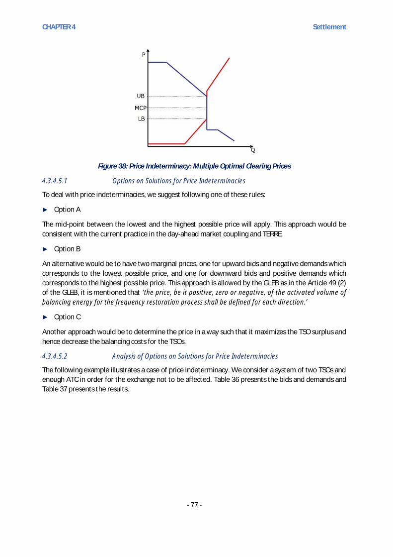
CHAPTER 4 Settlement
- 77 -
Figure 38: Price Indeterminacy: Multiple Optimal Clearing Prices
4.3.4.5.1 Options on Solutions for Price Indeterminacies
To deal with price indeterminacies, we suggest following one of these rules:
► Option A
The mid-point between the lowest and the highest possible price will apply. This approach would beconsistent with the current practice in the day-ahead market coupling and TERRE.
► Option B
An alternative would be to have two marginal prices, one for upward bids and negative demands whichcorresponds to the lowest possible price, and one for downward bids and positive demands whichcorresponds to the highest possible price. This approach is allowed by the GLEB as in the Article 49 (2)of the GLEB, it is mentioned that ‘the price, be it positive, zero or negative, of the activated volume ofbalancing energy for the frequency restoration process shall be defined for each direction.’
► Option C
Another approach would be to determine the price in a way such that it maximizes the TSO surplus andhence decrease the balancing costs for the TSOs.
4.3.4.5.2 Analysis of Options on Solutions for Price Indeterminacies
The following example illustrates a case of price indeterminacy. We consider a system of two TSOs andenough ATC in order for the exchange not to be affected. Table 36 presents the bids and demands andTable 37 presents the results.

CHAPTER 4 Settlement
- 78 -
Type Quantity(MWh)
TSO DemandPrice/Offer Price(€/MWh)
Elasticity ofDemand
Divisibility ofOffers
Demand (TSO 1) +100 -- Inelastic --Demand (TSO 2) -10 -- Inelastic --Upward Offer (UO BSP1) 100 5(TSO pays BSP) -- DivisibleDownward Offer (DOBSP2)
-10 7 (BSP pays TSO) -- Divisible
Table 36: Example Inputs
Type Activated Quantity/Satisfied Demand (MW)Demand (TSO 1) +100Demand (TSO 2) -10Upward Offer (UO BSP1) +100Downward Offer (UO BSP2) -10Social Welfare (€)15 Marginal Price (€/MWh)15
+200(= -500+700)
Output of algorithm: a value between 5 and 7Option A:6
Option B:5 for upward and 7for downward
Option C:5
Table 37: Example Outputs
We observe that all bids are fully activated and all demands are satisfied. The optimal price can beanything between 5€/MWh and 7€/MWh. Following Option 1, the result would be 6€/MWh as the mid-point would be chosen. Considering Option 2, the result would be 5€/MWh for upward bids (UO BSP 1)and negative demands (TSO 2), and 7€/MWh for downward bids (DO BSP 2) and positive demands (TSO1). Finally, Option 3 would result in a price of 5€/MWh, as in this way the total TSO surplus is maximized.
15 Calculation concept of social welfare optimization and derivation of marginal prices explained in chapter 3.2.2.1.

CHAPTER 4 Settlement
- 79 -
4.3.5 Questions
Q33. Do you prefer pricing option category A or B? Why?
Q34. Do you agree with the proposed criteria, weights and scoring for the assessment of pricingoptions? Why?
Q35. Would you consider additional pricing options? Why?
Q36. Which of the pricing options do you prefer? Why?
Q37. Which of the pricing options would incentivize you the most to submit Direct Activatable bids?Why?
Q38. Do you consider the issue of ”Rejected Scheduled bids/demand” to be problematic? Why?
Q39. Which of the three options regarding price indeterminacies would you prefer? Why?
4.3.6 Settlement of Netted Volumes
4.3.6.1 Definition of Netted Volumes
In order to avoid counter activation (simultaneous activation in opposite directions) of the balancingenergy, the demands on upward and downward mFRR will be netted within the cooperation area bytaking into account available cross-zonal capacities capacities. It means that an LFC area which is longsupplies energy to an LFC area which is short. In that way, the netting process enables all participatingTSOs to reduce mFRR activation as well as activation costs and leads thus to social welfare generationwithin the mFRR cooperation.
Table 38 illustrates the netting process between four LFC areas. LFC area A is short and would activate700 MWh positive mFRR whereas LFC areas B, C and D are long and would activate in total 600 MWhnegative mFRR. If there is no congestion, TSO A imports 600 MWh while TSO B exports 100 MWh, TSOC exports 200 MWh and TSO D exports 300 MWh. The residual mFRR demand of 100 MWh after nettingis covered by activating the cheapest bids of the upward common MOL. Thus due to the netting, themFRR demand can be reduced to 100 MWh and the netted energy results in avoided mFRR activation.
Indicator TSO A TSO B TSO C TSO DmFRR demand in MWh 700 -100 -200 -300Correction in MWh -600 100 200 300mFRR netting import in MWh 600 0 0 0mFRR netting export in MWh 0 100 200 300mFRR activation in MWh 100 0 0 0
Table 38: Netting of Opposed Activations
The netted volumes for each direction (separately for import and export) will be determined for eachTSO and for each quarter-hour.
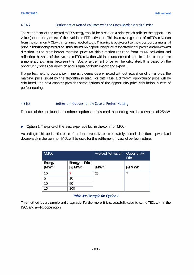
CHAPTER 4 Settlement
- 80 -
4.3.6.2 Settlement of Netted Volumes with the Cross-Border Marginal Price
The settlement of the netted mFRR energy should be based on a price which reflects the opportunityvalue (opportunity costs) of the avoided mFRR activation. This is an average price of mFRR activationfrom the common MOL within an uncongested area. This price is equivalent to the cross-border marginalprice in this uncongested area. Thus, the mFRR opportunity price respectively for upward and downwarddirection is the cross-border marginal price for this direction resulting from mFRR activation andreflecting the value of the avoided mFRR activation within an uncongested area. In order to determinea monetary exchange between the TSOs, a settlement price will be calculated. It is based on theopportunity prices per direction and is equal for both import and export.
If a perfect netting occurs, i.e. if inelastic demands are netted without activation of other bids, themarginal price issued by the algorithm is zero. For that case, a different opportunity price will becalculated. The next chapter provides some options of the opportunity price calculation in case ofperfect netting.
4.3.6.3 Settlement Options for the Case of Perfect Netting
For each of the hereinunder mentioned options it is assumed that netting avoided activation of 25MW.
► Option 1: The price of the least expensive bid in the common MOL
According to this option, the price of the least expensive bid (separately for each direction - upward anddownward) in the common MOL will be used for the settlement in case of perfect netting.
CMOL Avoided Activation OpportunityPrice
Energy[MWh]
Energy Price[€/MWh] [MWh] [€/MWh]
10 7 25 75 1010 5015 100
Table 39: Example for Option 1
This method is very simple and pragmatic. Furthermore, it is successfully used by some TSOs within theIGCC and aFRR cooperation.

CHAPTER 4 Settlement
- 81 -
► Option 2: Marginal price of avoided mFRR activation
This price corresponds to the cross-border marginal price resulting from a fictitious mFRR activation ifthe volumes would not have been netted but fully activated. The opportunity price of this option isusually higher than the price in option 1 (see Table 40).
CMOL Avoided Activation OpportunityPrice
Energy[MWh]
Energy Price[€/MWh] [MWh] [€/MWh]
10 7 25 505 1010 5015 100
Table 40: Example for Option 2
► Option 3: Average price of avoided mFRR activation
This price results from a fictitious mFRR activation if the volumes would not have been netted but fullyactivated as in option 2. Table 41 shows an example for the average price with the following calculation:
Opportunity price = Average price = (10 * 7 + 5 * 10 + 10 * 50)/(10 + 5 + 10) = 620/25 = 24,8
CMOL Avoided Activation OpportunityPrice
Energy[MWh]
Energy Price[€/MWh] [MWh] [€/MWh]
10 7 25 24,85 1010 5015 100
Table 41: Example for Option 3
In contrast to option 2, this is an average price from mFRR activation based on the pay-as-bid-settlement. The settlement price of this option is usually higher than the price in option 1 but lower thanin option 2.
► Option 4: Settlement based on avoided cost of mFRR activations in each area
The objective is to calculate the net welfare resulting from the perfect netting and to share equally thiswelfare. The welfare is calculated taking into account all the avoided costs in each control area.Following this, the welfare per TSO draws an opportunity price that is based on all the avoided costs ineach control area. In order to calculate the avoided costs of each TSO, the mFRR marginal price is usedthat would result from a fictitious activation in case that all TSOs had been isolated (e.g. local demandand local mFRR bids, with ll ATC=0), see Table 42 and the following calculation:

CHAPTER 4 Settlement
- 82 -
Opportunity costs TSO A = (10 + 5) * 10 = 150
Opportunity costs TSO B = 5 * 50 = 250
Opportunity costs TSO C = 5 * 60 = 300
Opportunity price = (150 + 250 + 300)/ (15 + 5 + 5) = 28
Then, there is a settlement applied to each control area.
MOLAvoidedActivation
MarginalPrice
OpportunityCosts
Totalwelfare
OpportunityPrice(welfare perMWh)
Energy[MWh]
EnergyPrice[€/MWh]
[MWh] [€/MWh] [€] [€] [€/MWh]
A 10 7 700 285 10 15 10 150
B 5 5015 653 70 5 50 250
C 5 6012 70 5 60 300
Table 42: Example for Option 4
This solution warrants that no TSO has a deficit. This is currently proposed in TERRE project.
► Option 5: Weighted average of DA/ID market price
DA or ID market price of each balancing area is used as a reference for the calculation of the settlementprice. Whereas this method is simple, it is not ensured that it will be positive for all the TSOs.
► Option 6: Predefined regulated price
This option implies application of a regulated price which should be approved by NRAs and reviewed ifnecessary. However, there are several questions that would have to be investigated for this option:
How to calculate this price? Will this be a fixed price for a whole period (e.g. month)?
How to ensure that it is GLEB compliant?
How to ensure that it will be positive for all the systems? And that benefits will be equally distributed?

CHAPTER 5 Congestion Management
- 83 -
Congestion Management
5.1 Introduction
This chapter tackles the issues and questions concerning congestion management, building on theprovisions of the GLEB on cross-zonal capacity calculation (Art. 37), i.e.:
1. After the intraday-cross-zonal gate closure time, TSOs shall continuously update theavailability of cross-zonal capacity for the exchange of balancing energy or for operating theimbalance netting process. Cross-zonal capacity shall be updated every time a portion of cross-zonal capacity has been used or when cross-zonal capacity has been recalculated.
2. Before the implementation of the capacity calculation methodology pursuant to paragraph 3,TSOs shall use the cross-zonal capacity remaining after the intraday cross-zonal gate closuretime.
3. 3. By five years after entry into force of this Regulation, all TSOs of a capacity calculation regionshall develop a methodology for cross-zonal capacity calculation within the balancingtimeframe for the exchange of balancing energy or for operating the imbalance nettingprocess. Such methodology shall avoid market distortions and shall be consistent with thecross-zonal capacity calculation methodology applied in the intraday timeframe establishedunder Commission Regulation (EU) 2015/1222.
Since the second paragraph stipulates that TSOs shall use the cross-zonal capacity remaining after theintraday cross-zonal gate closure time, we took the working assumption that the cross- zonal capacityto be used in the algorithm is the remaining capacity after intraday and also after RR process. The validityof this assumption will be critically examined again in the second phase of MARI design, especiallyregarding the interactions with other balancing processes such as aFRR. The working assumptions willbe reconsidered at the later stage according to the development of capacity calculation methodologies.
By dealing with congestion management, two main aspects are considered:
► The first purpose is that the TSOs shall make sure that bids that are activated for balancing purposeare not going to endanger the system security. The TSOs shall design an mFRR process and aplatform which guarantee that the system constraints are fully respected;
► Then, the second purpose is that a TSO may have a congestion management need to docountertrading or re-dispatch. In such case, the GLEB leaves open the possibility for the TSOs to usethe balancing platform to address TSO needs for countertrading or re-dispatch. In such caseadditional type of needs shall be considered in the mFRR process and platform.
In this report the focus is put on the congestion management constraints that shall be taken in accountby the platform when balancing need are covered by mFRR activated bids (see section 5.2).

CHAPTER 5 Congestion Management
- 84 -
5.2 Options to Handle Bottlenecks
When using the same area definition for mFRR as intraday some TSOs need additional measures tohandle congestions. The measures can be arranged before, within and/or after the algorithm calculation.The discussed measures are summarized and explained below.
1. TSOs limit ATC;
2. TSOs filter bids (mark them as unavailable);
3. Smaller internal mFRR zones in the mFRR algorithm;
4. Critical network elements in the mFRR algorithm;
5. Several TSOs form a cluster;
6. Re-dispatch the resulting flow after the mFRR algorithm.
According to the MARI Principles the Parties recognize that pragmatic congestion management handlingshould first be implemented in the mFRR Common Platform. Improved solutions should be jointlyassessed and implemented in a second step. This assessment should happen as soon as first operationalexperiences have been gained.
This implies that the first implementation of congestion management in the mFRR common platformshould open up for the TSOs to use their preferred measures to handle congestions, as long as themeasures do not require an implementation within the algorithm. The option evaluation will beelaborated as part of the design phase 2.
5.3 Analysis
5.3.1 Measures before Algorithm
5.3.1.1 Limiting ATC
To keep the transmission system within agreed security limits in the operational phase the TSOs has anopportunity to limit ATC after the ID market.
The measure creates an opportunity for a TSO to limit ATC for cross zonal capacity in order to handlecongestion management. This measure is common practice and currently used before intraday, RRprocess and in the IGCC cooperation. Each TSO update their ATC values and submit them to the platformbefore the TSO gate closure time.
The Figure 39 below shows how limiting ATC will affect the output from the clearing. A detaileddescription of this example can be found in Section 3.2.2.2/II.

CHAPTER 5 Congestion Management
- 85 -
Figure 39: Limiting ATC
The pros are that the measure is well-known, simple and needs no additional mechanism in thealgorithm when the measure is done in each TSO system. Furthermore this measure needs no directharmonisation.
This measure shall always be possible but only used if other measures are not suitable (or whileimproved solution is implemented). Limitation of cross-zonal capacity for purposes of congestionmanagement should be done in a coordinated and transparent way.
5.3.1.2 Filter Bids
The GLEB in its Article 29.14 states the following:
Each TSO may declare the balancing energy bids submitted to the activation optimisation functionunavailable for the activation by other TSOs because they are restricted due to internal congestion ordue to operational security constraints within the connecting TSO scheduling area.
This measure creates an opportunity for each TSO to filter bids that will create congestions by markingthem as unavailable before submitting them to the platform.
Figure 40: Bids Filtering
This is also a simple measure for which no additional mechanism in the algorithm and harmonisation isneeded. The measure is also foreseen in GLEB and shall therefore be foreseen anyhow. There shall be

CHAPTER 5 Congestion Management
- 86 -
sufficient time (to be assessed further) between BEGCT and TSO GCT, to let the TSO performing suchfiltering actions.
Information on unavailable bids has to be reported according to GLEB Art. 12(3)(b)(v).
5.3.2 Measures within Algorithm
5.3.2.1 Several Internal mFRR Zones within the Intraday Bidding Zone
In this measure the algorithm includes smaller areas than the intraday process, according to internalcongestions. The Figure 41 below depicts a simple case with three TSOs using internal zones. A moredetailed description can be found in Section 3.2.2.2./II.
Figure 41: Several Internal mFRR Zones within the Intraday Bidding Zone
The advantage of this option is that the higher resolution grid model will be used to guarantee a moreefficient method for dealing with external and/or internal congestion. This measure is more optimizedthan measures applying before the algorithm (cf. sections 5.3.1.1 and 5.3.1.2) but need to beinvestigated further in the following aspects: compliancy with GLEB, definition of ATC values, criteriaand limitations for the additional (smaller zones) and feasibility in such a small timeframe.
Implications on TSO-TSO settlement methodology (e.g. definition of uncongested area, sharing ofcongestion rent, etc.) and TSO-BSP settlement need to be investigated.
5.3.2.2 Critical Network Elements
Similar to the flow based approach in day-ahead, this approach is based on critical network elementsmonitoring and setting limits on the calculated flows on these elements influenced by mFRR balancingenergy exchanges. In this case a flow based congestion domain replaces ATCs, where flow based forIntraday and Balancing will be developed.

CHAPTER 5 Congestion Management
- 87 -
Figure 42: Critical Network Elements
The main principle of this approach is that a TSO has the possibility to monitor of the (approximated)change of the physical flow on predefined critical network elements and when necessary to set limits tothe induced physical flows on these predefined critical network element.
Further, during activation, the activation optimization function could consider limits on the inducedflows from MARI on these modeled critical network elements. Thus, a critical network element limitationshall be taken into account by the algorithm as an extra-constraint. The incorporation of theseconstraints and the monitoring would be performed via the usage of one PTDF matrix. The methodologyto define the critical elements that would be monitored and the associated PTDF matrix would have tobe further discussed..
The advantage of this option is that the higher resolution grid model will be used to guarantee a moreefficient method for dealing with external and/or internal congestion
The main difficulty of this option is to define the methodology to define the PTDF matrix including a gridmodel. Further, compliancy with GLEB, implications on TSO-TSO settlement methodology and TSO-BSPsettlement need to be investigated.
5.3.2.3 Several TSOs Form a Cluster16
Some TSOs have a need of representing their network model building a cluster together with other TSOs.If bids where to be activated within this cluster, bids from a certain TSO would be given priority over theother TSOs to a certain amount of MWs. The inputs to the algorithm include the control zones involved,the priority TSO and the amount of MW to be activated from this TSO are inputs from respective TSOsto the algorithm. The Figure 43 below illustrates this option and a detailed description can be found inSection 3.2.2.2/II.
16 This option will be further analysed with particular emphasis on the compliance with GLEB.

CHAPTER 5 Congestion Management
- 88 -
Figure 43: A Simple Example with Three TSOs Building a Cluster
This option could lead to social welfare reductions due to deviation from the merit order list.Additionally, the precedence of bids from a certain TSO over other TSOs could be seen as discriminatory.Further implications for settlement, level playing field and compliance with GLEB will be analysed at alater stage of the project.
5.3.3 Measures after Algorithm
5.3.4 Re-Dispatch
This measure creates an opportunity for the TSO to re-dispatch the resulting flow from the clearing. Thismeasure can be handled by re-dispatch using generation, consumption, topological changes and phaseshifting transformers. The TSO who block the activation of one bid selected by the platform shall providethe amount activated power in another way.
The Figure 44 below illustrates the option re-dispatch.
Figure 44: Re-Dispatch
This measure is simple and needs no additional mechanism in the algorithm when the measure is doneby each TSO.
This measure might not be compliant with GLEB Art. 29(6): Each connecting TSO shall ensure theactivation of the balancing energy bids selected by the activation optimisation function. On the otherhand, a situation may occur where a TSO needs to perform re-dispatch and cannot guarantee activatingthe bids selected by the optimisation function.

CHAPTER 5 Congestion Management
- 89 -
Moreover, the measure can be seen as economically suboptimal because it might require some bids tobe kept locally just as a back-up for bids that may or may not be activated on the platform.
5.4 Questions
Q40. Do you have specific comments regarding the congestion management options presented here?
Q41. Do you think that additional congestion management options are missing? If that is the case, couldyou please elaborate?

CHAPTER 6 Harmonization
- 90 -
Harmonization
6.1 Introduction
The GLEB aims at fostering an efficient, transparent and non-discriminatory pan European balancingmarket. To do so, it establishes certain rules and obligations for TSOs, BSPs, BRPs and other marketactors.
In order to achieve the objectives, the GLEB requires certain level of cooperation in the mentioned rulesso that the implementation of the balancing market provides an equal and fair treatment as well as alevel playing field for all the parties involved, especially the BSPs and the BRPs.
Nowadays, the balancing markets (and in particular the mFRR market) are very different from eachother, as they are strongly linked to the real operation of the system, which is, at the same time,conditioned by structural aspects such as, for example, the energy mix or the level of interconnections.Thus, all the systems will need to implement changes in order to achieve an integrated balancing marketin Europe.
In order to ensure a stable and reliable development, and to comply with the deadlines imposed by theGLEB for the implementation of the European platforms such as MARI, there should be a prioritizationamong all the rules and aspects of the balancing market. The aim of this chapter is to list the potentialaspects of harmonization under the scope of MARI project and to identify which of those would be mostimportant from the stakeholders’ point of view.

CHAPTER 6 Harmonization
- 91 -
6.2 Harmonization Requirements in the GLEB
The GLEB establishes several harmonization requirements such as:
► Framework for harmonization of terms and conditions for BSPs;► Framework for harmonization of terms and conditions for BRPs;► Implementation frameworks for European platforms for exchange of balancing energy;► Requirements for the exchange of balancing capacity;► List of standard products;► Gate Closure Times for submission of balancing bids;► Principles for Integrated Scheduling Process (for central dispatch systems);► Methodologies for activation of balancing energy bids;► Settlement rules;► Methodologies for the use of cross-zonal capacities (CZC);► Transparency requirements etc.
6.3 List of Potential Topics for Harmonization in MARI
Based on all the requirements of the GLEB, the MARI project is working on the identification of the mostimportant design features to be harmonized under the scope of MARI. In order to ease theunderstanding, the different items have been structured as follows:
Bid Characteristics
Considered Aspect for Harmonization Description► Maximum bid size The maximum size of a divisible or indivisible bid, which can
be offered at one time.► Price limits Existence of maximum and/or minimum price for the bid.► Requirements for Direct Activated
products and for Scheduledactivated products
Some TSOs perform mFRR process mainly based onscheduled products, while other would require more directactivated products
► Application of the “expectedshape” of a trapezoid with 10 minramps (up / down)
Although the algorithm optimizes the block of energy, theexpected shape to be delivered by the BSP should be atrapeze with 10 min ramps up/down
► Definition of the “acceptedshape” of the product
The local tolerance bands for bids for the delivered mFRRenergy accepted by the national TSOs
Settlement of TSO-BSPConsidered Aspect for Harmonization Description► Application of cross border
marginal price to the BSPactivated bid (= same as TSO-TSOprice);
Settlement to the BSP at the XBMP
► Energy settled (energycorresponding to the block ofenergy offered by the BSP);
Volume of energy taken into account for the settlement tothe BSP (energy corresponding to the activated bid)
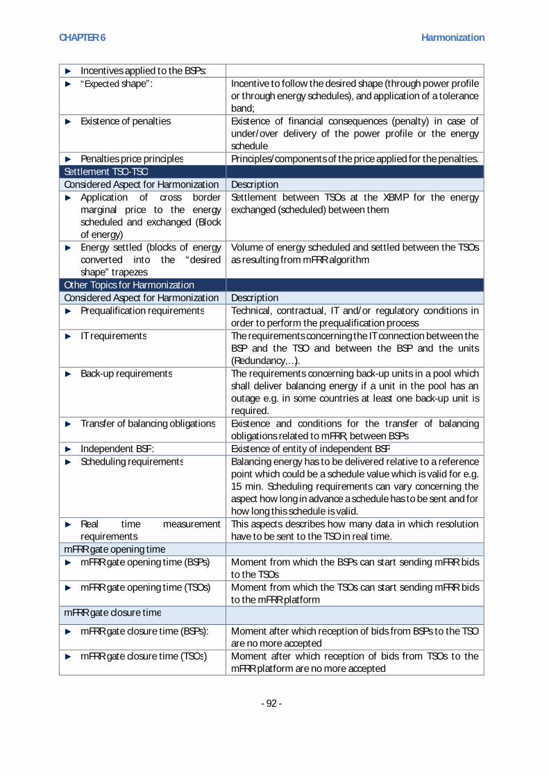
CHAPTER 6 Harmonization
- 92 -
► Incentives applied to the BSPs:► “Expected shape”: Incentive to follow the desired shape (through power profile
or through energy schedules), and application of a toleranceband;
► Existence of penalties Existence of financial consequences (penalty) in case ofunder/over delivery of the power profile or the energyschedule
► Penalties price principles Principles/components of the price applied for the penalties.Settlement TSO-TSOConsidered Aspect for Harmonization Description► Application of cross border
marginal price to the energyscheduled and exchanged (Blockof energy)
Settlement between TSOs at the XBMP for the energyexchanged (scheduled) between them
► Energy settled (blocks of energyconverted into the “desiredshape” trapezes
Volume of energy scheduled and settled between the TSOsas resulting from mFRR algorithm
Other Topics for HarmonizationConsidered Aspect for Harmonization Description► Prequalification requirements Technical, contractual, IT and/or regulatory conditions in
order to perform the prequalification process► IT requirements The requirements concerning the IT connection between the
BSP and the TSO and between the BSP and the units(Redundancy,…).
► Back-up requirements The requirements concerning back-up units in a pool whichshall deliver balancing energy if a unit in the pool has anoutage e.g. in some countries at least one back-up unit isrequired.
► Transfer of balancing obligations Existence and conditions for the transfer of balancingobligations related to mFRR, between BSPs
► Independent BSP: Existence of entity of independent BSP► Scheduling requirements Balancing energy has to be delivered relative to a reference
point which could be a schedule value which is valid for e.g.15 min. Scheduling requirements can vary concerning theaspect how long in advance a schedule has to be sent and forhow long this schedule is valid.
► Real time measurementrequirements
This aspects describes how many data in which resolutionhave to be sent to the TSO in real time.
mFRR gate opening time► mFRR gate opening time (BSPs) Moment from which the BSPs can start sending mFRR bids
to the TSOs► mFRR gate opening time (TSOs) Moment from which the TSOs can start sending mFRR bids
to the mFRR platformmFRR gate closure time
► mFRR gate closure time (BSPs): Moment after which reception of bids from BSPs to the TSOare no more accepted
► mFRR gate closure time (TSOs) Moment after which reception of bids from TSOs to themFRR platform are no more accepted

CHAPTER 6 Harmonization
- 93 -
► Nature of mFRR market: Nature of the mFRR energy market: obligation to offer intothe market or voluntary provision.
mFRR need:► Reasons for activating bids for
other purposes than balancinge. g. how to solve a congestion
► Transparency Transparency requirements from Transparency Regulationand from GLEB (common publications and Nationalpublications).
Table 43. Potential Harmonization Topics
6.4 Questions
Q42. Following the list of elements provided in this Chapter, could you indicate your top threeharmonization priorities?
Q43. In your opinion, which elements should be harmonized before the MARI project goes live?
Q44. In your opinion, which elements should foster harmonization, but not necessarily before the MARIproject goes live?
Q45. Apart from the elements mentioned in this Chapter, do you think other elements should beharmonized? If yes which ones?

ANNEX 1 Examples of Algorithm Constraints
- 94 -
ANNEX 1 - Examples of Algorithm Constraints
In this examples we assume the same sign conventions as well as assumptions for the shake of theexamples we took in Chapter 3 (i.e. the assumption for the technical price limit for the inelastic demand).
1) Power Balance Constraints
EXAMPLE 1:
In Example 1, there is a demand of +100 MWh. The accepted upward offers are 80 MWh of UO BSP1and 20 MWh of UO BSP3. Although UO BSP2 is a cheaper offer, it is not activated as it is an indivisiblebid (its activation of 21 MWh along with the activation of 80 MWh of UO BSP1 exceeds the demand ofTSO1 of 100 MW).
TYPE Quantity(MWh)
TSO Demand Price/Offer Price(€/MWh)
Elasticity of Demand Divisibility of Offers
Demand (TSO 1) +100 -- Inelastic --Upward Offer (UO BSP1) 80 10 -- Indivisible
Upward Offer (UO BSP2) 21 20 -- Indivisible
Upward Offer (UO BSP3) 30 30 -- Divisible
Table 44: Inputs for Example 1 - Maximization of Social Welfare & Netting
Type Activated Quantity/Satisfied Demand (MW)
Demand (TSO 1) +100Upward Offer (UO BSP1) 80Upward Offer (UO BSP2) 0Upward Offer (UO BSP3) 20Social Welfare (€) Marginal Price (€/MWh)
100·10000 - 80·10 - 20·30 - 100·30+ 80·30 + 20·30 = 998’600
30
Table 45: Output for Example 1
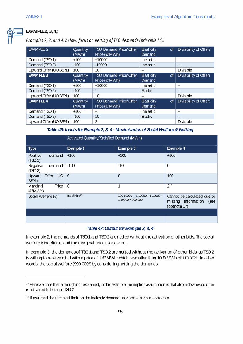
ANNEX 1 Examples of Algorithm Constraints
- 95 -
EXAMPLE 2, 3, 4,:
Examples 2, 3, and 4, below, focus on netting of TSO demands (principle I.C):
EXAMPLE 2 Quantity(MWh)
TSO Demand Price/OfferPrice (€/MWh)
Elasticity ofDemand
Divisibility of Offers
Demand (TSO 1) +100 +10000 Inelastic --Demand (TSO 2) -100 -10000 Inelastic --Upward Offer (UO BSP1) 100 10 -- DivisibleEXAMPLE 3 Quantity
(MWh)TSO Demand Price/OfferPrice (€/MWh)
Elasticity ofDemand
Divisibility of Offers
Demand (TSO 1) +100 +10000 Inelastic --Demand (TSO 2) -100 1 Elastic --Upward Offer (UO BSP1) 100 10 -- DivisibleEXAMPLE 4 Quantity
(MWh)TSO Demand Price/OfferPrice (€/MWh)
Elasticity ofDemand
Divisibility of Offers
Demand (TSO 1) +100 -- Inelastic --Demand (TSO 2) -100 10 Elastic --Upward Offer (UO BSP1) 100 2 -- Divisible
Table 46: Inputs for Example 2, 3, 4 - Maximization of Social Welfare & Netting
Activated Quantity/Satisfied Demand (MWh)
Type Example 2 Example 3 Example 4
Positive demand(TSO 1)
+100 +100 +100
Negative demand(TSO 2)
-100 -100 0
Upward Offer (UOBSP1)
0 0 100
Marginal Price(€/MWh)
0 1 217
Social Welfare (€) Indefinite18 100·10000 - 1·10000 +1·10000 -1·10000 = 990’000
Cannot be calculated due tomissing information (seefootnote 17)
Table 47: Output for Example 2, 3, 4
In example 2, the demands of TSO 1 and TSO 2 are netted without the activation of other bids. The socialwelfare isindefinite, and the marginal price is also zero.
In example 3, the demands of TSO 1 and TSO 2 are netted without the activation of other bids, as TSO 2is willing to receive a bid with a price of 1 €/MWh which is smaller than 10 €/MWh of UO BSP1. In otherwords, the social welfare (990 000€ by considering netting the demands
17 Here we note that although not explanied, in this example the implicit assumption is that also a downward offeris activated to balance TSO 2
18 If assumed the technical limit on the inelastic demand: 100·10000 + 100·10000 = 2’000’000

ANNEX 1 Examples of Algorithm Constraints
- 96 -
In example 4, the demands of TSO 1 and TSO 2 are not netted, as TSO 2 is willing to receive a price of 10€/MWh which is higher than 2 €/MWh of UO BSP1. The social welfare in order to be determined wouldneed to know the price of DO in order to satisfy the TSO 1 demand.Power Flow Constraints
EXAMPLE 5, 6
Through examples 5 and 6, described below, we illustrate the outcome of the algorithm for the casewith only ATC values and the case with internal zones involved.
Figure 45 shows a scheme for a simple system where three areas representing by three TSOs are linkedtogether through ATC values in red.19 Considering offers and demands in Table 48, the outcomes areprovided in Table 49.
Figure 45: A Simple Example with Three TSOs Involved with ATC. Values in Red are ATC Limits.
19 We should note that all four German TSOs can represent one area of Germany with the corresponding ATCvalues with neighboring countries.

ANNEX 1 Examples of Algorithm Constraints
- 97 -
Type Quantity(MWh)
TSO DemandPrice/OfferPrice (€/MWh)
Elasticity ofDemand
Divisibility ofOffers
Area
Positive demand (TSO1)
+100 +10000 Inelastic -- Area 1
Positive demand (TSO2)
+100 +10000 Inelastic -- Area 2
Negative demand (TSO3)
-200 -10000 Inelastic -- Area 3
Upward Offer (UOBSP1)
100 10 -- Divisible Area 1
Upward Offer (UOBSP2)
30 20 -- Divisible Area 2
Downward Offer (UOBSP2)
-50 -20 -- Divisible Area 2
Downward Offer (DOBSP3)
-200 -50 -- Divisible Area 3
Table 48: Inputs for Example 5 – Respecting Power Flow Constraint in term of ATC
As shown in Figure 45, TSO 3 can have in total 80 MW exchange with TSO 1 and TSO 2.
To obtain the maximum social welfare (i.e., minimum balancing cost) while respecting the powerbalance constraint (total supply equals to total demands.) and power flow constraints, the optimaloutcome includes the activation of upward offers UO BSP1 (full 100 MW) and UO BSP2 (20 MW of 30MW), as well as downward offer DO BSP3 (-120 MW of -200MW).. These activated amounts along with80 MW netted amount ensure the power balance equations while respecting ATC limits.
Due to ATC limits, a power exchange larger than 80 MW is not possible between area 3 and the rest ofthe system. This leads to two marginal prices: one in areas 1 and 2 (20 €/MWh) and the other one inarea 3 (50 €/MWh).
Type Activated Quantity/Satisfied Demand (MWh)
Positive demand (TSO 1) +100Positive demand (TSO 2) +100Negative demand (TSO 3) -200Upward Offer (UO BSP1) 100Upward Offer (UO BSP2) 20Downward Offer (UOBSP2)
0
Downward Offer (DOBSP3)
-120
Social Welfare (€) XB Marginal Price (€/MWh)+100*10’000 +100*10’000+200*10’000 -(10*100+20*20)+(-120*50)=3’992’600(
Area 1 & 2:20 €/MWh
Area 3:50 €/MWh
Table 49: Output for Example 5

ANNEX 1 Examples of Algorithm Constraints
- 98 -
As shown in Figure 46, example 6 illustrates a simple case where TSO 1 expresses its power flow limitsthrough ATC whereas TSO 2 and TSO 3 express their power flow limits through a number of zones. Ifthere is a cross- zonalcapacity between different zones illustrated with a blue line, the correspondingcross- zonal capacity limit is assumed to be 10 MW in this example. We should note that since there isno line between zone 4 and zone 5, there is no possibility of exchange between these two zones in thisexample.
Figure 46: A Simple Example with Three TSOs Involved with ATC Values and Zones.
The inputs for Example 6 are provided in Table 50.
Type Quantity(MWh)
TSO DemandPrice/OfferPrice(€/MWh)
Elasticity ofDemand
Divisibilityof Offers
Area
Positive demand (TSO 1) +100 +10000 Inelastic -- Area 1Positive demand (TSO 2) +80 +10000 Inelastic -- Zone 1Positive demand (TSO 2) +20 +10000 Inelastic -- Zone 3Negative demand (TSO 3) -50 -10000 Inelastic -- Zone 4Negative demand (TSO 3) -150 -10000 Inelastic -- Zone 5Upward Offer 1 (UO1 BSP1) 100 10 -- Divisible Area 1Upward Offer 2 (UO2 BSP2) 10 15 -- Divisible Zone 1Upward Offer 3 (UO3 BSP2) 50 20 -- Divisible Zone 2Upward Offer 4 (UO4 BSP2) 20 50 -- Divisible Zone 3Downward Offer 5 (DO5 BSP3) -50 -40 -- Divisible Zone 4Downward Offer 6 (DO6 BSP3) -150 -50 -- Divisible Zone 5
Table 50: Inputs for Example 6, Respecting Power Flow Constraint in Term of ATC and Zones

ANNEX 1 Examples of Algorithm Constraints
- 99 -
Type Activated Quantity/Satisfied Demand (MWh)
Positive demand (TSO 1) +100Positive demand (TSO 2) +80Positive demand (TSO 2) +20Negative demand (TSO 3) -50Negative demand (TSO 3) -150Upward Offer 1 (UO1 BSP1) 100Upward Offer 2 (UO2 BSP2) 10Upward Offer 3 (UO3 BSP2) 10Upward Offer 4 (UO4 BSP2) 0Downward Offer 5 (DO5 BSP3) -10Downward Offer 6 (DO6 BSP3) -110Social Welfare (€) XB Marginal Price (€/MWh)
(100+80+20+50+150)*10000-(100*10+10*15+10*20+10*40+110*50)= 4’000’000 – 7250 = 3’995’750
Area1
Zone 1 Zone2
Zone3
Zone4
Zone5
20 20 20 0 40 50
Table 51: Output for Example 6.
The following demands are simultaneously netted and compensated by acceptance of offers in thealgorithm:
► Area 1: +100-20 = +80 (netting of demands TSO 1 and TSO 3 Zone 5 with limit of 20 MWh)
Activation of UO1
► Zone 1:
+80-20 = +60 (netting of demands TSO 2 zone 1 and TSO 3 Zone 5 with limit of 20 MWh)
+60-20 = +40 (netting of demands TSO 3 Zone 4 through Zone 3 to Zone 1 = 20 MWh)
Activation of UO1 & UO2 & UO3
Therefore, Area 1 and Zones 1 and 2 have the same marginal price driven by activation of UO3 (nocongestion appears between these areas).
► Zone 3: +20-20 = 0 (netting of demands TSO 2 zone 3 and TSO 3 zone 4)
No Activation of offersà marginal price of zero
► Zone 4: -50+40 = -10 (netting of demands TSO 2 zone 3, TSO 2 zone 1 and TSO 3 zone 4)
Activation of DO5à marginal price of 40 €/MWh
► Zone 5: -150+20+20 = -110 (netting of demands TSO 1, TSO 2 zone 1 and TSO 3 Zone 5 with a totallimit of 40 MWh)
Activation of DO6à marginal price of 50 €/MWh

ANNEX 1 Examples of Algorithm Constraints
- 100 -
EXAMPLE 7 – TSO building a Cluster
Figure 47: A Simple Example with Three TSOs Building a Cluster
The inputs for example 7 are provided in Table 52.
Type Quantity(MWh)
TSO DemandPrice/OfferPrice(€/MWh)
Elasticityof Demand
Divisibilityof Offers
Area Priorityvolume
Demand (TSO 1) 0 -- Inelastic -- Area 1 0
Demand (TSO 2) 0 -- Inelastic -- Area 2 +120
Positive demand (TSO3)
+200 -- Inelastic -- Zone 3 0
Upward Offer 1 (UO1BSP1)
+100 10 -- Divisible Area 1
Upward Offer 2 (UO2BSP2)
+120 15 -- Divisible Area 2
Table 52: Inputs for Example 7 – TSOs Build a Cluster
Type Activated Quantity/Satisfied Demand (MWh)
Demand (TSO 1) +0
Demand (TSO 2) +0
Demand (TSO 3) +200
Upward Offer 2 (UO2 BSP2) +120
Upward Offer 1 (UO1 BSP1) +80
Social welfare (€) XB Marginal Price (€/MWh)
200*10000-(120*15+80*10) = 2000000 –2600 = 1’997’400
Same Marginal price for the Cluster = 15
Table 53: Output for Example 7

ANNEX 1 Examples of Algorithm Constraints
- 101 -
2) HVBC Constraints Example:
EXAMPLE 8:
In the following example, the losses on the HVDC link are characterized by a percentage (4 %) of thecirculating flow inside the interconnector. This percentage entirely determines the line’s losses, andshould be applied in both directions, whether A or B is the exporting area. Thus, when A wants to export1000 MWh, only 960 MWh actually reaches market area B.
Figure 48: Example of Power Flow Losses on an HVDC Link
To take into account these physical losses, the algorithm should provide two specific features: somespecific power flow constraints, and a specific output price computation. These two features can bedirectly inspired from what has been done in the Euphemia algorithm for DA market coupling. Theyshould of course be completed with an appropriate settlement process regarding the congestion rentmanagement, as again in the current example of the Euphemia algorithm.
EXAMPLE 9:
· Power flow results from the algorithm in ISP1 = 600 MWh· Max ramp (input to the algorithm) = 300 MW (ramp speed 30 MW/minute and 10 minute
ramping time)· Therefore, to respect the flow in this HVDC line in ISP2, the limit is calculated using a given input
of a max ramp of 300 MW and considering the flow of this line from the previous clearinginterval. That is, the power flow must be within limits from 600-300 = 300 MW to 600+300=900MWh
EXAMPLE 10:
· Input data for TSO:· CZC =±500 MWh· Already allocated flow in previous clearing Area A -> Area B = 100 MWh· Technical minimum power = ± 50 MWh· Input data for AOF:· CZCB Area A -> Area B 400 MW (500 MWh - 100 MWh)· CZCB Area B -> Area A 600 MW (500 MWh + 100 MWh)· Not allowed balancing power exchange flow from Area B to Area A at an interval of [100-50
100+50] MWh= [50 150] MWh.

ANNEX 1 Examples of Algorithm Constraints
- 102 -
Figure 49: HVDC Dynamics Constraints

ANNEX 2 List of Tables
- 103 -
ANNEX 2 – List of Tables
Table 1: mFRR Product Definition (the marking * means that the values follow current discussion at theENTSO-E level; the marking ** meants that it is related to the FAT) .................................................... 11Table 2: Direct Deactivation ................................................................................................................ 17Table 3 : Summary of Activation Alternatives ...................................................................................... 21Table 4: Comparison of the Two Options for a Maximum Bid Size of Indivisible Bids Representing a Small(Option 1) and a Big (Option 2) Maximum Bid Size............................................................................... 26Table 5: Demand Structure .................................................................................................................. 34Table 6: Example - Cost Curve Formed by Offers/Bids and Elastic Demands ......................................... 35Table 7: Inputs for Example - Activation of Bids with the Aim of Maximization of Social Welfare ......... 38Table 8: Output for Example ................................................................................................................ 38Table 9: Inputs for Example 10 - Unforeseen Rejected Divisible Bids .................................................... 41Table 10: Output for Example 10 ......................................................................................................... 42Table 11: Criteria for Qualitative Evaluation of Allowing/Avoiding Unforeseen Rejected Divisible Bidsfrom the Algorithm Point of View ........................................................................................................ 43Table 12: UAB Example: Input Data ..................................................................................................... 44Table 13: Example Input Data .............................................................................................................. 45Table 14: Example Input ATC ............................................................................................................... 48Table 15. Evaluation Criteria for Allowing or Restricting Counter-Activations ....................................... 49Table 16: Inputs for Example ............................................................................................................... 51Table 17: Output for Example .............................................................................................................. 51Table 18: Inputs for Example ............................................................................................................... 52Table 19: Output for Example .............................................................................................................. 52Table 20: Theoretical Example without Congestion ............................................................................. 56Table 21: Financial Flows without Congestion ..................................................................................... 56Table 22: Reference Data for Example with Congestion ....................................................................... 58Table 23: Financial Flows with Congestion ........................................................................................... 58Table 24: Criteria for Volume Options.................................................................................................. 64Table 25: Assessment of Volume Settlement Option 1......................................................................... 65Table 26: Assessment of Volume Settlement Option 2......................................................................... 65Table 27: Criteria for Pricing Options ................................................................................................... 67Table 28: Definitions for Table of Criteria for Pricing Options ............................................................... 68Table 29: Pricing Options ..................................................................................................................... 70Table 30: Assessment of Pricing Options.............................................................................................. 70Table 31: Comparison of the Options which Meet All Must-Criteria ..................................................... 71Table 32: Formulas of Shortlisted Options ........................................................................................... 72Table 33: Example of Counter-Directactivation Due to Absence of Netting .......................................... 74Table 34: Example of Counter-Directactivation involving SA bids ......................................................... 74Table 35: Pricing Options ..................................................................................................................... 76Table 36: Example Inputs .................................................................................................................... 78Table 37: Example Outputs .................................................................................................................. 78Table 38: Netting of Opposed Activations ............................................................................................ 79Table 39: Example for Option 1 ........................................................................................................... 80

ANNEX 2 List of Tables
- 104 -
Table 40: Example for Option 2 ........................................................................................................... 81Table 41: Example for Option 3 ........................................................................................................... 81Table 42: Example for Option 4 ........................................................................................................... 82Table 43. Potential Harmonization Topics ............................................................................................ 93Table 44: Inputs for Example 1 - Maximization of Social Welfare & Netting ......................................... 94Table 45: Output for Example 1 ........................................................................................................... 94Table 46: Inputs for Example 2, 3, 4 - Maximization of Social Welfare & Netting .................................. 95Table 47: Output for Example 2, 3, 4 ................................................................................................... 95Table 48: Inputs for Example 5 – Respecting Power Flow Constraint in term of ATC ............................ 97Table 49: Output for Example 5 ........................................................................................................... 97Table 50: Inputs for Example 6, Respecting Power Flow Constraint in Term of ATC and Zones ............. 98Table 51: Output for Example 6. .......................................................................................................... 99Table 52: Inputs for Example 7 – TSOs Build a Cluster ........................................................................ 100Table 53: Output for Example 7 ......................................................................................................... 100
ANNEX 3 List of Figures
- 105 -
ANNEX 3 – List of Figures
Figure 1: Elements of the Product Shape ...............................................................................................8Figure 2: mFRR Product Physical Shape SA.............................................................................................9Figure 3: mFRR Product Physical Shape Longest DA ...............................................................................9Figure 4: Illustration of the Shape of the Cross-Border Exchange for a Scheduled Activation (left part)and Various Direct Activations (right part) ........................................................................................... 10Figure 5: Timing of the Scheduled Process ........................................................................................... 13Figure 6: Example of Activation with 5-Minute Cycles for Direct Activation (the shape of the cross-borderexchange is shown) ............................................................................................................................. 15Figure 7: Example of Activation with 1 Minute Cycles for Direct Activation .......................................... 16Figure 8: Alternative 1 - Direct Activation before Scheduled Activation for Two Consecutive QHs ....... 18Figure 9: Alternative 2 - Scheduled before Direct Activation for Two Consecutive QHs ....................... 19Figure 10: Scheduled Activation before Direct Activation with Deactivation in QH0 and QH1 .............. 19Figure 11: Scheduled Activation before Direct Activation with Deactivation in QH0 ............................. 20Figure 12: Possible Links between Bids ................................................................................................ 22Figure 13: Scheme of Activation Optimization Function ....................................................................... 32Figure 14: An Example of Cost Curve Formed by Bids and Elastic Demands ......................................... 35Figure 15: Social Welfare ..................................................................................................................... 37Figure 16: UAB Example: Merit Order List ............................................................................................ 44Figure 17: Merit Order List .................................................................................................................. 45Figure 18: Example Merit Order List .................................................................................................... 46Figure 19: Example Activations ............................................................................................................ 46Figure 20: Scheduled Counter-Activations’ Restriction: Impact on Merit Order List.............................. 47Figure 21: Scheduled Counter-Activations’ Restriction: Impact on Activations ..................................... 47Figure 22: Impact of a Congestion on Counter-Activations ................................................................... 48Figure 23: A Restriction of Scheduled Counter-Activation Increases the Marginal Price ....................... 49Figure 24: A Restriction of Scheduled Counter-Activation Decreases the Marginal Price ...................... 49Figure 25: Cost Curve Formed by Offers and Elastic Demands.............................................................. 54Figure 26: Local vs. Common Merit Order List, without Congestion ..................................................... 55Figure 27: Settlement without Congestion........................................................................................... 55Figure 28: Local vs. Common Merit Order List, with Congestion........................................................... 57Figure 29: Settlement with Congestion ................................................................................................ 57Figure 30: XBMP vs. Local Imbalance Pricing ........................................................................................ 61Figure 31: Assumed Exchange Profiles of Scheduled and Direct Activation .......................................... 63Figure 32: Volume Option1 for SA ....................................................................................................... 64Figure 33: Volume Option 1 for DA ...................................................................................................... 64Figure 34: Volume Option 2 for SA and DA .......................................................................................... 65Figure 35: Rejection of Scheduled Bids ................................................................................................ 72Figure 36: Social Welfare Loss in Case of TSOs Which Only Use SA, Elastic SA Needs and a Clearing PriceIncl. DA................................................................................................................................................ 73Figure 37: Counter-Activations, Example ............................................................................................. 75Figure 38: Price Indeterminacy: Multiple Optimal Clearing Prices ........................................................ 77Figure 39: Limiting ATC ........................................................................................................................ 85

ANNEX 3 List of Figures
- 106 -
Figure 40: Bids Filtering ....................................................................................................................... 85Figure 41: Several Internal mFRR Zones within the Intraday Bidding Zone ........................................... 86Figure 42: Critical Network Elements ................................................................................................... 87Figure 43: A Simple Example with Three TSOs Building a Cluster.......................................................... 88Figure 44: Re-Dispatch ........................................................................................................................ 88Figure 45: A Simple Example with Three TSOs Involved with ATC. Values in Red are ATC Limits. .......... 96Figure 46: A Simple Example with Three TSOs Involved with ATC Values and Zones. ............................ 98Figure 47: A Simple Example with Three TSOs Building a Cluster........................................................ 100Figure 48: Example of Power Flow Losses on an HVDC Link................................................................ 101Figure 49: HVDC Dynamics Constraints .............................................................................................. 102

ANNEX 4 List of Abbreviations
- 107 -
ANNEX 4 - List of Abbreviations
AC Alternating Current
ACE Area Control Error
aFRR Automatic Frequency Restoration
AOF Activation Optimization Function
ATC Available Transmission Capacities
BEGCT Balancing Energy Gate Closure Time
BRP Balancing Responsible Party
BSP Balancing Service Provider
CACM Guideline on Capacity Allocation and Congestion Management
CB Control Block
CCRs Capacity Calculation Regions
CID Congestion Income Distribution
CM Congestion Management
CMOL Common Merit Order List
CZC Cross-Zonal Capacity
DA Direct Activation, directly activated, directly activatable
DO Downward Offer
EBGL Electricity Balancing Guideline
EC European Commission
EPDA Earliest Point of Direct Activation
FAT Full Activation Time
FB Flow-based
FCR Frequency Containment Reserves
FRCE Frequency Restoration Control Error
FRP Frequency Restoration Process
GCT Gate Closure Time
GLSO Guideline on Electricity Tranmission System Operation
GLEB Guideline on Electricity Balancing
HVDC High Voltage Direct Current
ID Intraday (Market)

ANNEX 4 List of Abbreviations
- 108 -
IGCC International Grid Control Cooperation
ISP Imbalance Settlement Period
LB Lower Boundary
LFC Load Frequency Control(ler)
LPDA Latest Point of Direct Activation
MARI Manually Activated Reserves Initiative
MC Market Coupling
MCP Market Clearing Price
MEAS Mutual Emergency Assistance Service
mFRR Manual Frequency Restoration Reserves
MOL Merit Order List
MoU Memorandum of Understanding
MP Marginal Price
NRA National Regulatory Authority
NTC Net Transmission Capacity
PTDF Power Transfer Distribution Factor
QH Quarter Hour
REMIT Regulation on Wholesale Energy Market Integrity and Transparency
RR Replacement Reserves
SA Scheduled Activation, scheduled activated, scheduled activatable
SCADA Supervisory Control and Data Acquisition
SOC Systém Operation Committee
TERRE Trans-European Replacement Reserves Exchange
TSO Transmission System Operator
TTRF Time to restore Frequency
UAB Unforseeably Accepted Bids
UB Upper Boundary
UO Upward Offer
WG AS Working Group Ancillary Services under ENTSO-E
XB Cross-Border
XBMP Cross-Border marginal pricing