Marginal Deterrence at Work�

Rosario Crinoy Giovanni Immordinoz Salvatore Piccolox

April 28, 2017

Abstract

We test the rational economic model of marginal deterrence of law enforcement

� i.e., the need for graduating the penalty to the severity of the crime. We use

a unique data set, which combines individual-level data on sentence length for a

representative sample of US inmates with proxies for maximum punishment and

monitoring costs across US states over 50 years. We show that the penalty is in-

creasing in the level of the o¤ense. Consistent with the marginal deterrence frame-

work, we also document that a decrease in maximum penalty or an increase in

monitoring cost are associated with longer sentences and higher monitoring rates.

We also provide evidence that the e¤ects of maximum penalty and monitoring cost

are stronger in states where income inequality is higher. Finally, we show that

steeper sanctions are associated with less harmful crimes. Overall, these �ndings

favor the marginal deterrence framework over the maximal penalty principle and

other competing theories of justice.

JEL Classification: K14, K40.

Keywords: Marginal Deterrence, Enforcement Policies, Individual-Level Data,

Death Penalty.

�We thank Giuseppe Dari-Mattiacci for useful comments. Pietro Panizza and Enrico Turco providedexcellent research assistance. Financial support from the Einaudi Institute for Economics and Finance isgratefully acknowledged. The usual disclaimer applies.

yUniversità Cattolica del Sacro Cuore, Department of Economics and Finance; CEPR; and CESifo.E-mail: rosario.crino@unicatt.it.

zUniversità Federico II di Napoli, Department of Economics and Statistics; and CSEF. Email: gio-vanni.immordino@unina.it

xUniversità di Bergamo, Department of Management and Economics; and CSEF. Email: salva-tore.piccolo@unibg.it

1. Introduction

Since the pioneering work by Becker (1968), law enforcement has attracted considerable

attention by economists, and for good reasons. The development of e¢ cient enforcement

systems is inextricably linked with economic growth, �nancial development and the rise

of modern democracies. Designing �good�laws is, in fact, not enough to guarantee these

objectives without an e¤ective deterrence.

Several prominent scholars in law and economics have, over the past decades, debated

intensively on the notion of optimal enforcement of law. In models where agents simply

consider whether to commit a single harmful act or not, the threat of severe sanctions

is enough to deter people from infringing the law: the maximal punishment principle

(Becker, 1968). Yet, when agents can also choose the severity of the harm their actions

in�ict to society, �hanging people for a sheep�might not be a good idea (Friedmand and

Sjostrom, 1993). Notably, undeterred individuals will have a reason to commit less, rather

than more harmful acts, if expected sanctions rise with harm. This tendency is sometimes

said to re�ect marginal deterrence � i.e., the need for graduating penalties to the severity

of the harm.

Yet, even if the anecdotal evidence seems to corroborate the idea that penalties are

sensitive to the severity of harm, it is surprising that the empirical literature on this issue

is rather narrow, despite the intense theoretical debate, and that it lacks a systematic

analysis of the practical relevance of marginal deterrence as opposed to competing theories.

In order to �ll this gap, in this paper we investigate empirically if, and to what extent, the

rational economic model of marginal deterrence of law enforcement provides a reasonable

description of the enforcement policies actually chosen by regulators and law enforcers.

As shortly explained before, older theoretical contributions on these issues have as-

sumed that each individual chooses whether or not to commit one act � i.e., the �single-

act� framework developed in Becker (1968), Landes and Posner (1975), Polinsky and

Shavell (1984) and Friedman (1981), among others. However, starting from the seminal

contribution by Stigler (1970), the literature has recognized the role of marginal deter-

rence. The logic behind this theory is fairly intuitive: stepping up enforcement against

one level of the activity may induce a switch to a more harmful act instead. Friedman

and Sjostrom (1993), Mookherjee and Png (1992, 1994), Reinganum and Wilde (1986),

Shavell (1991, 1992), and Wilde (1992) study the conditions under which the presence of

marginal deterrence induces optimal penalties that are graduated to the severity of the

harm produced by di¤erent law infringements.

Our objective is three-fold. First, we provide evidence of a systematic correlation

2

between penalties and harm severity, which provides prima facie evidence for the marginal

deterrence approach. Second, in order to argue that in real life penalties actually re�ect

marginal deterrence we test the main implications of the theory underlying the logic of

marginal deterrence. Third, we show that steeper sanctions induce less harmful crimes.

Speci�cally, the analysis endeavours to answer the following questions. Are actual

punishments (Reinganum and Wilde, 1986; Shavell, 1992; Wilde, 1992) and their ex-

pected values (Friedman and Sjostrom, 1993; Mookherjee and Png, 1994) higher for more

severe crimes? While these are general predictions of the marginal deterrence frame-

work, they also apply to other non-economic based theories of justice, according to which

penalties should not re�ect deterrence. For example, a positive relationship between

punishments and harm severity would obtain also when penalties are set according to

a retributive principle.1 Hence, in order to clarify whether a positive correlation be-

tween penalties and harm severity can be rationalized with marginal deterrence, we also

test some comparative-statics predictions o¤ered by the general environment analyzed by

Mookherjee and Png (1994). Speci�cally, is it true that if the maximum possible punish-

ment drops or if the cost of monitoring increases the regulator should reduce the expected

penalties on all illegal acts?

While evidence of a positive relationship between maximum punishment and expected

penalties would bring support to marginal deterrence, one could argue that a similar pat-

tern can be generated by a punishment logic based on retribution. Essentially, as long as

crimes are punished proportionally to the harm they generate, optimal penalties in states

in which the maximum punishment is higher should be (on average) higher than penalties

in other states, because courts in the former states should be relatively more likely to

apply tougher standards than courts in the latter. Yet, while this e¤ect seems to give

rise to a parallel shift of penalties in states with higher maximum punishment, this is not

the case with marginal deterrence, as we document below. In addition, and even more

convincingly, evidence of a negative correlation between monitoring cost and expected

penalties would unambiguously point in the direction of marginal deterrence, since com-

peting theories of justice would posit that penalties should not feature this dependence.

In sum, testing these relationships also allows us to provide the �rst assessment of the

empirical validity of the marginal deterrence principle as opposed to the maximal penalty

principle and to other competing theories of justice.

To perform the empirical analysis, we build a novel and unique data set, which com-

1Retributive justice is a theory of justice postulating that the best response to a crime should onlyre�ect the social harm of the crime rather than extrinsic social purposes such as deterrence, rehabilitationof the o¤ender etc. (see, e.g., Perry, 2006).

3

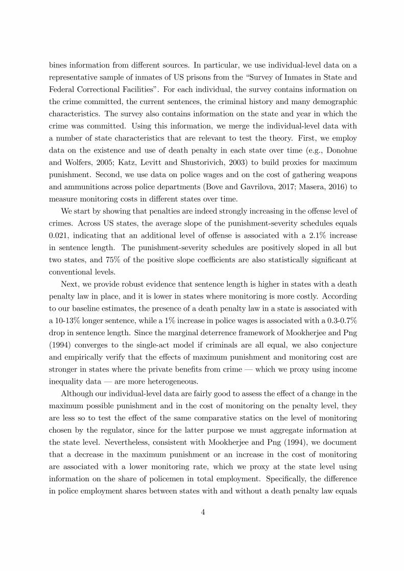
bines information from di¤erent sources. In particular, we use individual-level data on a

representative sample of inmates of US prisons from the �Survey of Inmates in State and

Federal Correctional Facilities�. For each individual, the survey contains information on

the crime committed, the current sentences, the criminal history and many demographic

characteristics. The survey also contains information on the state and year in which the

crime was committed. Using this information, we merge the individual-level data with

a number of state characteristics that are relevant to test the theory. First, we employ

data on the existence and use of death penalty in each state over time (e.g., Donohue

and Wolfers, 2005; Katz, Levitt and Shustorivich, 2003) to build proxies for maximum

punishment. Second, we use data on police wages and on the cost of gathering weapons

and ammunitions across police departments (Bove and Gavrilova, 2017; Masera, 2016) to

measure monitoring costs in di¤erent states over time.

We start by showing that penalties are indeed strongly increasing in the o¤ense level of

crimes. Across US states, the average slope of the punishment-severity schedules equals

0.021, indicating that an additional level of o¤ense is associated with a 2.1% increase

in sentence length. The punishment-severity schedules are positively sloped in all but

two states, and 75% of the positive slope coe¢ cients are also statistically signi�cant at

conventional levels.

Next, we provide robust evidence that sentence length is higher in states with a death

penalty law in place, and it is lower in states where monitoring is more costly. According

to our baseline estimates, the presence of a death penalty law in a state is associated with

a 10-13% longer sentence, while a 1% increase in police wages is associated with a 0.3-0.7%

drop in sentence length. Since the marginal deterrence framework of Mookherjee and Png

(1994) converges to the single-act model if criminals are all equal, we also conjecture

and empirically verify that the e¤ects of maximum punishment and monitoring cost are

stronger in states where the private bene�ts from crime � which we proxy using income

inequality data � are more heterogeneous.

Although our individual-level data are fairly good to assess the e¤ect of a change in the

maximum possible punishment and in the cost of monitoring on the penalty level, they

are less so to test the e¤ect of the same comparative statics on the level of monitoring

chosen by the regulator, since for the latter purpose we must aggregate information at

the state level. Nevertheless, consistent with Mookherjee and Png (1994), we document

that a decrease in the maximum punishment or an increase in the cost of monitoring

are associated with a lower monitoring rate, which we proxy at the state level using

information on the share of policemen in total employment. Speci�cally, the di¤erence

in police employment shares between states with and without a death penalty law equals

4

16% of the sample mean of this variable; at the same time, a 1% increase in police wages

across states is associated with a reduction in the monitoring rate of approximately 2%

of the sample mean.

Finally, we provide evidence on the e¤ectiveness of marginal deterrence. The latter

requires penalties to be graduated to harms, so as to avoid criminals switching to more

harmful acts. Accordingly, if marginal deterrence works, we should expect steeper sanc-

tions to be associated with less harmful crimes. Indeed, we �nd that in states where

punishment-severity schedules are steeper, an increase in the slope of this schedule is as-

sociated with a signi�cant reduction in the average o¤ense level. Moreover, we �nd that

steeper schedules are associated with relatively fewer inmates committing more serious

crimes.

Our analysis is obviously related to the literature on the determinants of crime, which

has studied the role of direct policies such as the size of the police force,2 the incarcera-

tion rate3 and capital punishment,4 as well as the e¤ect of more indirect factors such as

abortion5 or gun laws.6 Unlike all these papers, we do not investigate the determinants of

crime, but we rather focus on the determinants of the enforcement policies meant to �ght

it. Speci�cally, we show that the enforcement policies and the toughness of sanctions

in di¤erent US states are by and large consistent with the rational economic model of

marginal deterrence of law enforcement.

The rest of the paper is organized as follows. Section 2 summarizes the empirical

predictions of marginal deterrence for optimal punishment. Section 3 describes the data.

Section 4 presents the baseline results. Section 5 reports some robustness checks. Section 6

extends the analysis to the monitoring rate and to the role of inequality. Section 7 provides

additional evidence on the e¤ectiveness of marginal deterrence. Section 8 concludes.

2. Theoretical Background

To begin with, in order to gain intuition on the empirical strategy that we will develop

in the next sections, we shortly summarize the basic logic of the model developed by

2See for instance Cameron (1988), Cornwell and Trumbell (1994), Di Tella and Schargrodsky (2004),Moody and Marvell (1996), Levitt (1996) and McCrary (2002).

3See for instance Abrams (2006), Chen and Shapiro (2004), Drago et al. (2009), Johnson and Raphael(2006), Kessler and Levitt (1999), Levitt (1996) and Webster, Doob and Zimring (2006).

4See among others Cohen-Cole et al. (2009), Donohue and Wolfers (2005), Ehrlich (1975, 1977), Katz,Levitt and Shustorivich (2003) and Passell and Taylor (1977).

5See among others Dills and Miron (2006), Donohue and Levitt (2001, 2004, 2008), Foote and Goetz(2008), Joyce (2003, 2009) and Lott and Whitley (2007).

6See Ayres and Donohue (2003a, 2003b), Black and Nagin (1998), Helland and Tabarrok (2004), Lottand Mustard (1997), Lott (1998, 2003) and Plassmann and Whitley (2003).

5

Mookherjee and Png (1994), which provides the most general environment to study mar-

ginal deterrence of enforcement of law. Mookherjee and Png (1994) study a model in

which the level of the criminal activity is a continuous variable, and individuals derive

heterogeneous bene�ts from infringing the law. In their baseline analysis, they consider an

environment in which, although the monitoring system detects all acts at a common rate,

regardless of their harmfulness, acts of di¤ering severity may be penalized at di¤erent

rates. The policy they consider speci�es both a monitoring rate and penalties. For given

policy, each individual will choose an harmful act to maximize the di¤erence between the

bene�ts from infringing the law � which are heterogeneous � and the expected penalty

for the act � which is type independent. A consequence is that higher types � i.e., those

who bene�t the most from a harmful act � cannot choose less harmful acts. In the limit

when all individuals derive the same bene�ts from infringing the law (no heterogeneity)

the model converges to the single-act framework, where only one harmful act is chosen in

equilibrium.

In this environment the authors characterize the optimal policy for a regulator that

maximizes an utilitarian welfare function, which attributes equal weight to private bene-

�ts, external harms and enforcement costs. The model does not allow for in�nitely large

punishments, otherwise any desired pattern of deterrence could be achieved at minimal

cost by combining arbitrarily low monitoring with su¢ ciently steep penalties. The mon-

itoring rate is assumed to be non-contingent on the severity of the harm produced by

criminals, whereas penalties are contingent on it.7

If enforcement were costless and the regulator could distinguish individuals� types,

each individual would be induced to choose the �rst-best action, namely, the one that

trades o¤ each individual�s marginal bene�t against the corresponding marginal harm.

This decision rule changes when enforcement becomes costly and when the regulator can-

not distinguish individuals�types: the second best features a distortion that is standard

in adverse selection environments à la Mirlees and re�ects how costly monitoring is, the

heterogeneity of the pro�tability of crime across individuals as well as the maximal pun-

ishment that the society can in�ict to law breakers.

In a nutshell, the analysis o¤ered by Mookherjee and Png (1994) shows that � in a

marginal deterrence setting � if society wishes to reduce the harmful act chosen by a

given individual, it necessarily must raise expected penalties for all more harmful acts.

7This is an important assumption in this and other models of marginal deterrence (see also Rein-ganum and Wilde, 1986; Shavell, 1992; Wilde, 1992). All these papers assume that the probabilities ofapprehension (monitoring rate in Mookherjee and Png, 1994) for two or more alternative harmful acts aredetermined by the same decision, so the only way of changing the expected penalty for one act withoutchanging the expected penalty for another is by altering the actual penalty.

6

Penalties, however, cannot be raised beyond the given maximum. Hence, it is not optimal

to match the �rst-best degree of deterrence for any type.

In this setting, an increase in the maximum possible penalty increases the scope for

deterrence through the means of higher penalties. The same increase in the scope for

deterrence results from a fall in the monitoring cost. Intuitively, when monitoring (hence

deterrence) becomes less costly, society should move closer to the �rst-best pattern of

deterrence, stepping up expected penalties for all illegal acts.

Using the data described in the next section, in Section 4 we will test the following

predictions:

Prediction 1. The optimal actual punishment for a crime is higher for more severecrimes.

Reinganum and Wilde (1986), Shavell (1992) and Wilde (1992) investigate the question

of whether the optimal punishment rises with the seriousness of the o¤ense. Provided

that the probability of actual punishment is not decreasing in the seriousness of the crime

� as it is typically the case in reality � our results also support the conclusions of

Friedman and Sjostrom (1993) and Mookherjee and Png (1994), who show theoretically

that the expected punishment (i.e., the combination of probability and actual punishment)

is increasing in the level of o¤ense.8

Prediction 2. If the maximum possible punishment is higher, the regulator should, otherthings being equal, increase the expected penalty on all illegal acts.

Prediction 3. If the cost of monitoring is higher, the regulator should, other things beingequal, reduce the expected penalty on all illegal acts.

Although Predictions 2 and 3 are stated in terms of expected penalty, we will rather look at

actual punishment. The reason is twofold. First, by looking at actual punishment we can

fully exploit our individual-level information on a large sample of inmates of US prisons,

and control for a large set of individual and state confounders in the empirical analysis.

To calculate expected penalty we must instead aggregate information at the state level (an

exercise that we do later on as a robustness check) and thus rely on stronger assumptions

for identi�cation. Second, in Section 6 we show that if the maximum possible punishment

is higher, or if the cost of monitoring is lower, the regulator increases the monitoring

8As underlined by Friedman and Sjostrom (1993) if a given crime is punished in expected terms moreseverely than another crime, this does not necessarily imply that the actual punishment for the �rst crimeis also higher. From a theoretical point of view, some extra assumptions are required.

7

rate. Therefore, if both the monitoring rate and the actual punishment go in the right

direction, the same must be true for the combination of the two � i.e., the expected

punishment. Interestingly, our strategy allows us to compare empirically the marginal

deterrence model with the single-act one. In the single-act framework of Polinsky and

Shavell (1992) an increase in the cost of monitoring should reduce monitoring and raise

penalties. We �nd, instead, that such an increase reduces both monitoring and penalties

in accordance with the marginal deterrence framework.

3. Data and Descriptive Evidence

3.1. Data

To test the theoretical predictions laid down in the previous section, we assemble a unique

data set by combining information from di¤erent sources. We draw individual-level data

on a nationally-representative sample of inmates of US prisons from the latest wave of

the �Survey of Inmates in State and Federal Correctional Facilities�. This survey was run

by the Bureau of Justice Statistics in 2004 across inmates of State and Federal prisons.

For each individual, the survey reports information on his/her current o¤ense, current

sentence, criminal history, demographic characteristics, family background, and weapon,

drugs and alcohol use. The total number of interviewed inmates is 18,185. Out of these,

we focus on the subsample of 7,963 individuals who (i) are currently sentenced to serve

time, (ii) have not received either a life or a death sentence (as in these cases we could

not compute sentence length), and (iii) for whom we have complete information on all

the variables used in the analysis.

The �Survey of Inmates in State and Federal Correctional Facilities� also contains

information on the state in which each criminal committed his/her o¤ense and on the

year of arrest. Using this information, we merge the individual-level data with a number

of state characteristics that are relevant to test the theoretical predictions of marginal

deterrence. First, we use information on death penalty to construct proxies for the max-

imum penalty applied in each state and year. We obtain information on the existence of

a death penalty law from the �Death Penalty Information Center�. As shown in Table 1,

the existence of a death penalty law varies markedly across states and time. Speci�cally,

four states (Maine, Michigan, Minnesota and Wisconsin) never had a death penalty law

in place over our sample period (1953-2003), while in the remaining states, the number

of years in which a death penalty law was in place ranges from 4 (Alaska and Hawaii)

to 50 (Arkansas, Arizona, Connecticut, Florida, Georgia, Indiana, Louisiana, Nebraska,

8

Nevada, Oklahoma and Utah).9 We complement the information on the existence of a

death penalty law with data on the number of actual capital executions in each state

and year, sourced from the �Death Penalty Information Center�. As shown in Table 1,

there is large variation also in this variable, with the cumulated number of executions

ranging from 0 (in 19 states) to 313 (in Texas) over the sample period. Second, to con-

struct our main proxy for monitoring cost, we use the monthly wage of policemen in each

state and year. We source this information for the period 1982-2003 from the �Criminal

Justice Expenditure and Employment Extracts�of the Census Bureau �Annual Govern-

ment Finance Survey�and �Annual Survey of Public Employment�. Following Bove and

Gavrilova (2017) and Masera (2016), we also use alternative proxies based on the physical

cost faced by police departments in each state for gathering military equipment (details

below).

3.2. Descriptive Statistics

Table 2 reports descriptive statistics on the individual characteristics. The inmates in our

sample were arrested over a period of 50 years, from 1953 to 2003. Their average age is

36 and their sentence length equals 4,438 days (roughly 12 years) on average. The vast

majority (79%) of inmates are males and US born (88%). The number of white and black

inmates is roughly equivalent (49% and 42%, respectively), as is the number of married

and divorced individuals (20% and 21%, respectively). The majority of inmates (68%)

have a high-school diploma, but we also observe a substantial share of individuals with

either a university degree (17%) or just primary education (12%). One-quarter of inmates

are held in Federal prisons and the remaining three-quarters in State prisons. One-�fth

of inmates have a parent who was sentenced in the past, and roughly 15% of them have

spent some time in jail before the current sentence. Almost one-fourth of individuals have

used a weapon during the o¤ense.

The last three rows of the table report information on the o¤ense level of crimes

committed by inmates. We obtain this information from Chapter 2 of the �US Federal

Sentencing Guidelines Manual�, which sets rules for a uniform sentencing of individuals

who are convicted to felonies and serious misdemeanors (punished with at least one year

of prison) in the US Federal court system. The Guidelines assign to each crime one of

43 base o¤ense levels. We manually map the description of the crime committed by each

inmate (as provided in the survey) to one of these o¤ense levels. As shown in Table 2,

9These 11 states reintroduced the death penalty after suspending it for one year in 1972, following the�Furman�decision by the U.S. Supreme Court, which deemed capital punishment unconstitutional andtransformed all pending death sentences to life imprisonment.

9

more than 50% of crimes have o¤ense levels between 12 and 22 - e.g., marijuana or hashish

tra¢ cking (o¤ense level of 13), attempted sexual assault (17) and unarmed robbery (21).

The frequency of less and more serious crimes is lower.

3.3. Punishment-Severity Schedules

We now study how sentence length varies across o¤ense levels. According to Prediction

1, more severe crimes should be punished with longer sentences. Thus, in Figure 1a we

plot the median sentence length across all inmates on the 43 o¤ense levels. We normalize

all sentences by the sentence length of the �rst o¤ense level. The relation is sharply

increasing, with the median sentence of the most severe crimes exceeding that of the least

severe o¤enses by 20 times.

In Figure 1b we repeat the exercise after controlling for observable characteristics of

the inmates. To this purpose, we start by regressing the log sentence length (number of

days) on demographic, crime and state-level controls, plus a full set of year dummies. The

demographic controls are age and its square, gender, race and marital status dummies,

indicators for US born inmates and for inmates with sentenced parents, dummies for

educational levels and for inmates who ever served in the US Armed Forces, and an

indicator for inmates of Federal prisons. The criminal record controls are a dummy for

use or possession of weapons during the o¤ense, an indicator for whether the inmate spent

any time in other correctional facilities before the arrest, and a dummy for whether the

inmate ever used heroin. Finally, the state-level covariates are the shares of Catholics,

Protestants and Muslims in the state adult population, the state unemployment rate,

the log population of the state, the number of violent crimes, robberies and property

crimes per state inhabitant, and the state GDP. Then, we compute the residuals from

this regression, exponentiate them, and plot the median of the resulting variable on the

43 o¤ense levels. The main evidence is now even stronger.

Next, we estimate state-speci�c punishment-severity schedules, in order to study

whether the aggregate relationship documented in the previous graphs also holds across

individual states. To this purpose we regress, separately for each state, log sentence length

on o¤ense level (a variable ranging from 1 to 43 depending on the severity of the crime),

plus demographic and crime controls and a time trend. We restrict to states with at

least 40 inmates, so as to have enough degrees of freedom. The coe¢ cients on o¤ense

level obtained from these regressions give the slopes of the state-speci�c schedules. These

coe¢ cients indicate by how much sentence length changes (in percentage) in a given state

for each additional level of o¤ense. The results are displayed in Figure 2. Across all

10

states, the average slope equals 0.021, indicating that sentence length increases by 2.1%

on average for each additional level of o¤ense. The slopes range from -0.048 to 0.047.

However, they are positive in all but two states, and 28 (75%) of the positive slopes are

also statistically signi�cant at conventional levels.10 Overall, these results indicate that

the positive relationship between sentence length and o¤ense level is a robust relationship

across US states. In Section 7 we will use the estimated state-speci�c slopes presented in

this section to provide additional evidence on the e¤ectiveness of marginal deterrence.

4. Baseline Results

In this section, we test Predictions 2 and 3. To this purpose, we estimate various speci-

�cations in which the log sentence length is regressed on proxies for either the maximum

punishment (Prediction 2) or the cost of monitoring (Prediction 3) in the state and year

in which a given crime was committed. In our main analysis we focus on inmates whose

sentences are longer than 365 days, so as to make sure that our results are not driven

by very small sentences, whose duration may be noisy; as shown below, our results are

however robust to using alternative samples of di¤erent sentence length. Our main proxy

for maximum punishment is the existence of a death penalty law in a given state and year.

As our main measure of monitoring cost we use instead the monthly wage of policemen

in each state and year.

The results are reported in Tables 3 and 4. We start, in column (1), by regressing the

log sentence length on each proxy, controlling for full sets of dummies for the year of arrest

and for the 43 o¤ense levels. Accordingly, our identi�cation strategy consists of comparing

inmates who have committed crimes of similar severity within a given year, across states

characterized by di¤erent levels of maximum punishment and monitoring cost. Given that

the existence of a death penalty law and the police wage vary across states and years,

whereas the length of sentence is individual speci�c, we correct the standard errors for

clustering within state-year pairs. Consistent with Predictions 2 and 3, the results show

a positive coe¢ cient on the death penalty dummy and a negative coe¢ cient on the police

wage, implying that sentences are longer in states where the maximum punishment is

higher or the cost of monitoring is lower.

In the remaining columns, we include further controls to account for di¤erences across

inmates in observable characteristics, which may a¤ect the length of sentence. Speci�cally,

10The only states for which the slope is negative are Utah and Massachusetts, although the slope isstatistically signi�cant only in the former state. These results may partly re�ect the limited sample size,which equals 42 inmates for Utah and 56 for Massachusetts.

11

in column (2) we add controls for demographic characteristics. These are: age and age

squared; gender, race and marital status dummies; dummies for US born inmates and

for inmates with sentenced parents; dummies for educational levels; and dummies for

inmates who ever served in the US Armed Forces or are held in Federal prisons. In

column (3) we add controls for the criminal record of inmates, namely, a dummy for

use or possession of weapons during the o¤ense, a dummy for whether the inmate spent

any time in other correctional facilities before arrest, and a dummy for whether the

inmate ever used heroin. Finally, in column (4) we add state-level covariates, namely,

the shares of Catholics, Protestants and Muslims in the state adult population, the state

unemployment rate, GDP and population, and the number of violent crimes, robberies

and property crimes per state inhabitant. The main evidence is preserved across the

board. Quantitatively, our estimates for the death penalty coe¢ cient range between 0.10

and 0.13, implying that in states with a death penalty law, sentences are 10-13% longer

than in other states. Similarly, the estimated coe¢ cients on the police wage range between

0.3 and 0.7, implying that a 1% increase in police wages is associated with a 0.3-0.7%

drop in sentence length.

5. Robustness Checks

We now submit the baseline results to an extensive sensitivity analysis, which aims at

showing that our main evidence is preserved when using alternative proxies and estimation

samples, when accounting for possible underlying trends, and when exploiting di¤erent

identi�cation strategies.

5.1. Alternative Proxies

We start by showing that our baseline evidence holds across alternative proxies for the

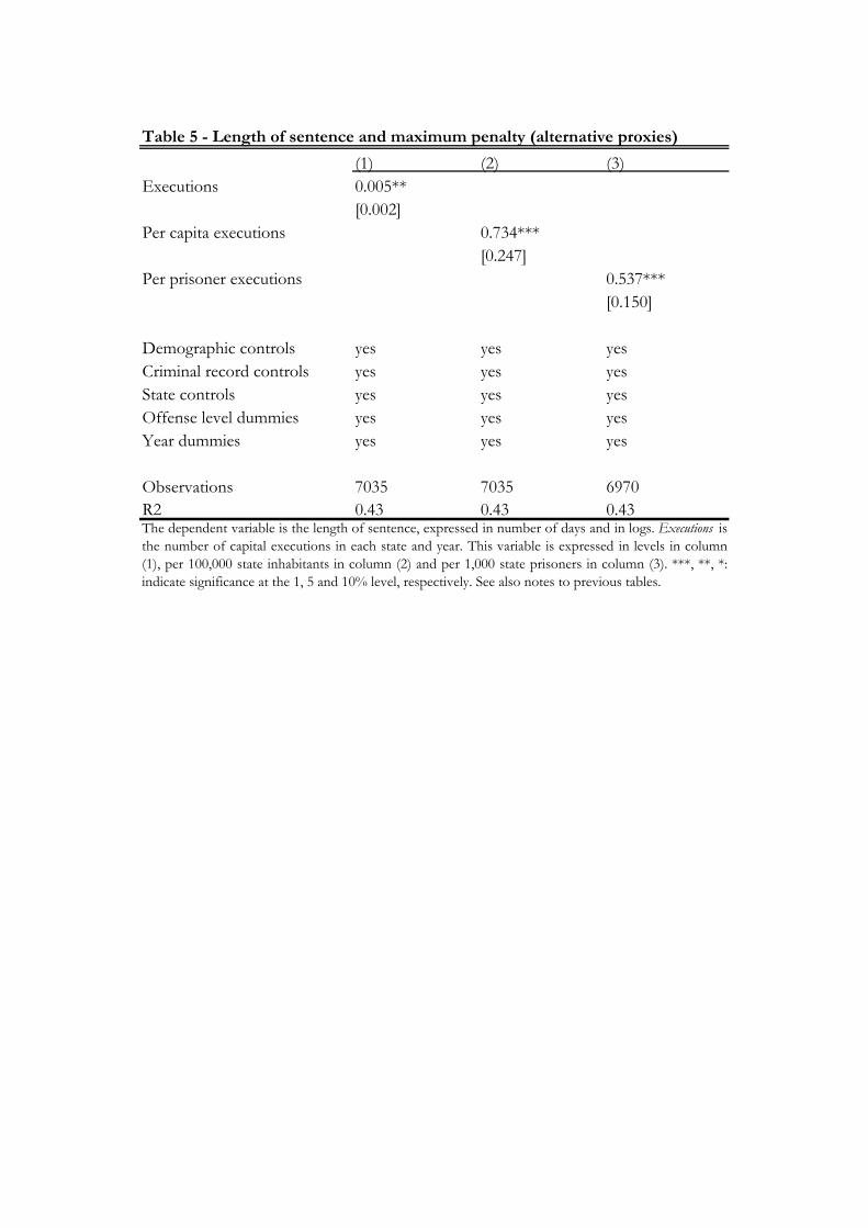
maximum penalty and the cost of monitoring. The results are reported in Tables 5 and 6.

As for the maximum penalty, we switch from the simple existence of a death penalty law to

a measure of its actual adoption. In particular, following a large empirical literature (e.g.,

Donohue and Wolfers, 2005; Katz, Levitt and Shustorivich, 2003), we use the number of

executions in a given state and year. We include this variable either in levels (column 1),

or per 100,000 state inhabitants (column 2), or per 1,000 state prisoners (column 3). In

all cases, we �nd that a more intensive use of the death penalty is associated with longer

sentences. Quantitatively, an increase in executions equal to the di¤erence between the

10th and the 90th percentile of the distribution (i.e., 17 executions) implies a 8.5% longer

12

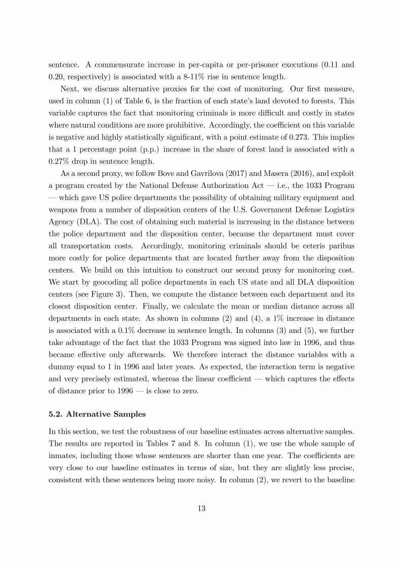
sentence. A commensurate increase in per-capita or per-prisoner executions (0.11 and

0.20, respectively) is associated with a 8-11% rise in sentence length.

Next, we discuss alternative proxies for the cost of monitoring. Our �rst measure,

used in column (1) of Table 6, is the fraction of each state�s land devoted to forests. This

variable captures the fact that monitoring criminals is more di¢ cult and costly in states

where natural conditions are more prohibitive. Accordingly, the coe¢ cient on this variable

is negative and highly statistically signi�cant, with a point estimate of 0.273. This implies

that a 1 percentage point (p.p.) increase in the share of forest land is associated with a

0.27% drop in sentence length.

As a second proxy, we follow Bove and Gavrilova (2017) andMasera (2016), and exploit

a program created by the National Defense Authorization Act � i.e., the 1033 Program

� which gave US police departments the possibility of obtaining military equipment and

weapons from a number of disposition centers of the U.S. Government Defense Logistics

Agency (DLA). The cost of obtaining such material is increasing in the distance between

the police department and the disposition center, because the department must cover

all transportation costs. Accordingly, monitoring criminals should be ceteris paribus

more costly for police departments that are located further away from the disposition

centers. We build on this intuition to construct our second proxy for monitoring cost.

We start by geocoding all police departments in each US state and all DLA disposition

centers (see Figure 3). Then, we compute the distance between each department and its

closest disposition center. Finally, we calculate the mean or median distance across all

departments in each state. As shown in columns (2) and (4), a 1% increase in distance

is associated with a 0.1% decrease in sentence length. In columns (3) and (5), we further

take advantage of the fact that the 1033 Program was signed into law in 1996, and thus

became e¤ective only afterwards. We therefore interact the distance variables with a

dummy equal to 1 in 1996 and later years. As expected, the interaction term is negative

and very precisely estimated, whereas the linear coe¢ cient � which captures the e¤ects

of distance prior to 1996 � is close to zero.

5.2. Alternative Samples

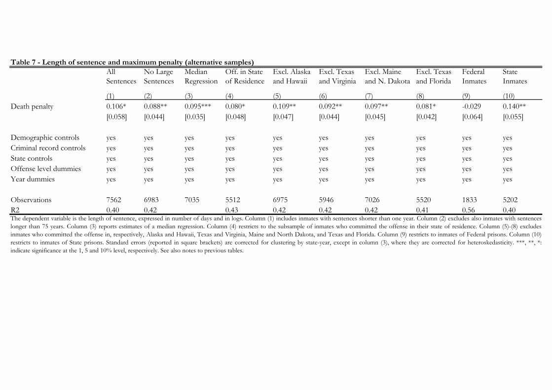
In this section, we test the robustness of our baseline estimates across alternative samples.

The results are reported in Tables 7 and 8. In column (1), we use the whole sample of

inmates, including those whose sentences are shorter than one year. The coe¢ cients are

very close to our baseline estimates in terms of size, but they are slightly less precise,

consistent with these sentences being more noisy. In column (2), we revert to the baseline

13

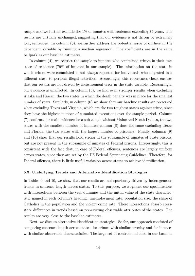
sample and we further exclude the 1% of inmates with sentences exceeding 75 years. The

results are virtually unchanged, suggesting that our evidence is not driven by extremely

long sentences. In column (3), we further address the potential issue of outliers in the

dependent variable by running a median regression. The coe¢ cients are in the same

ballpark as our baseline estimates.

In column (4), we restrict the sample to inmates who committed crimes in their own

state of residence (79% of inmates in our sample). The information on the state in

which crimes were committed is not always reported for individuals who migrated in a

di¤erent state to perform illegal activities. Accordingly, this robustness check ensures

that our results are not driven by measurement error in the state variable. Reassuringly,

our evidence is una¤ected. In column (5), we �nd even stronger results when excluding

Alaska and Hawaii, the two states in which the death penalty was in place for the smallest

number of years. Similarly, in column (6) we show that our baseline results are preserved

when excluding Texas and Virginia, which are the two toughest states against crime, since

they have the highest number of cumulated executions over the sample period. Column

(7) con�rms our main evidence for a subsample without Maine and North Dakota, the two

states with the smallest number of inmates; column (8) does the same excluding Texas

and Florida, the two states with the largest number of prisoners. Finally, columns (9)

and (10) show that our results hold strong in the subsample of inmates of State prisons,

but are not present in the subsample of inmates of Federal prisons. Interestingly, this is

consistent with the fact that, in case of Federal o¤enses, sentences are largely uniform

across states, since they are set by the US Federal Sentencing Guidelines. Therefore, for

Federal o¤enses, there is little useful variation across states to achieve identi�cation.

5.3. Underlying Trends and Alternative Identi�cation Strategies

In Tables 9 and 10, we show that our results are not spuriously driven by heterogeneous

trends in sentence length across states. To this purpose, we augment our speci�cations

with interactions between the year dummies and the initial value of the state character-

istic named in each column�s heading: unemployment rate, population size, the share of

Catholics in the population and the violent crime rate. These interactions absorb cross-

state di¤erences in trends based on pre-existing observable attributes of the states. The

results are very close to the baseline estimates.

Next, we discuss alternative identi�cation strategies. So far, our approach consisted of

comparing sentence length across states, for crimes with similar severity and for inmates

with similar observable characteristics. The large set of controls included in our baseline

14

speci�cations and robustness checks allays concerns with omitted variables potentially

correlated with sentence length, maximum punishment and monitoring cost. One may

still be concerned, however, that our results are driven by unobserved heterogeneity across

states. To address this concern, in panel a) of Tables 11 and 12, we re-estimate our main

speci�cations including state �xed e¤ects, which absorb time-invariant di¤erences across

states. We also control for a full set of US Census division-year �xed e¤ects, which absorb

time-varying di¤erences across states located in di¤erent areas.11 The coe¢ cients are now

identi�ed using time variation in sentences, death penalty and police wage within states,

after controlling for common shocks to states belonging to the same region. Our evidence

is unchanged and the coe¢ cients are slightly larger than before.

In panel b), we instead run Instrumental Variables regressions, in a further attempt

to isolate the exogenous variation of our main regressors. Following a vast empirical liter-

ature (surveyed, e.g., in Donohue and Wolfers, 2005), we instrument death penalty using

the share of votes cast for the Republican candidate in each state during the most recent

Presidential election. We instrument instead the police wage using the average wage paid

in the private non-farm sector of the state. As shown in column (12), both instruments

have strong predictive power in the �rst stage, and the second-stage coe¢ cients remain

similar to our baseline OLS estimates. In column (13) we show that neither instrument

has an independent e¤ect on sentence length after controlling for the endogenous regres-

sors, pointing in favor of the exclusion restriction. Finally, column (14) reports results

from a reduced-form speci�cation, in which sentence length is regressed directly on the

instruments. Consistent with previous results, we �nd sentences to be longer in states

with a larger Republican share or with lower private wages.

6. Extensions

6.1. Monitoring

As already mentioned, our individual-level data is fairly good for assessing the e¤ect

of a change in the maximum punishment and in the cost of monitoring on sentence

11Census divisions are nine groups of states de�ned as follows. Division 1 (New England): Connecticut,Maine, Massachusetts, New Hampshire, Rhode Island and Vermont. Division 2 (Middle Atlantic): NewJersey, New York and Pennsylvania. Division 3 (East North Central): Illinois, Indiana, Michigan, Ohioand Wisconsin. Division 4 (West North Central): Iowa, Kansas, Minnesota, Missouri, Nebraska, NorthDakota and South Dakota. Division 5 (South Atlantic): Delaware, District of Columbia, Florida, Georgia,Maryland, North Carolina, South Carolina, Virginia and West Virginia. Division 6 (East South Central):Alabama, Kentucky, Mississippi and Tennessee. Division 7 (West South Central): Arkansas, Louisiana,Oklahoma and Texas. Division 8 (Mountain): Arizona, Colorado, Idaho, Montana, Nevada, New Mexico,Utah and Wyoming. Division 9 (Paci�c): Alaska, California, Hawaii, Oregon and Washington.

15

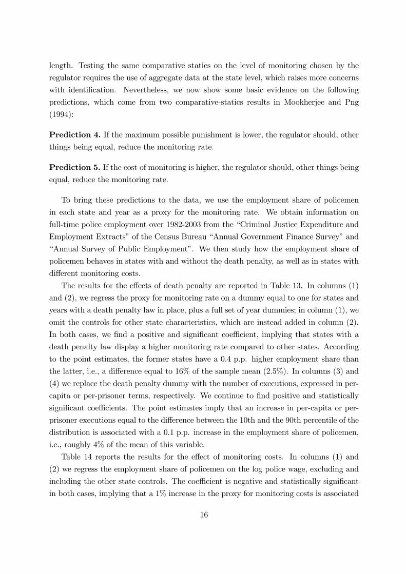
length. Testing the same comparative statics on the level of monitoring chosen by the

regulator requires the use of aggregate data at the state level, which raises more concerns

with identi�cation. Nevertheless, we now show some basic evidence on the following

predictions, which come from two comparative-statics results in Mookherjee and Png

(1994):

Prediction 4. If the maximum possible punishment is lower, the regulator should, otherthings being equal, reduce the monitoring rate.

Prediction 5. If the cost of monitoring is higher, the regulator should, other things beingequal, reduce the monitoring rate.

To bring these predictions to the data, we use the employment share of policemen

in each state and year as a proxy for the monitoring rate. We obtain information on

full-time police employment over 1982-2003 from the �Criminal Justice Expenditure and

Employment Extracts�of the Census Bureau �Annual Government Finance Survey�and

�Annual Survey of Public Employment�. We then study how the employment share of

policemen behaves in states with and without the death penalty, as well as in states with

di¤erent monitoring costs.

The results for the e¤ects of death penalty are reported in Table 13. In columns (1)

and (2), we regress the proxy for monitoring rate on a dummy equal to one for states and

years with a death penalty law in place, plus a full set of year dummies; in column (1), we

omit the controls for other state characteristics, which are instead added in column (2).

In both cases, we �nd a positive and signi�cant coe¢ cient, implying that states with a

death penalty law display a higher monitoring rate compared to other states. According

to the point estimates, the former states have a 0.4 p.p. higher employment share than

the latter, i.e., a di¤erence equal to 16% of the sample mean (2.5%). In columns (3) and

(4) we replace the death penalty dummy with the number of executions, expressed in per-

capita or per-prisoner terms, respectively. We continue to �nd positive and statistically

signi�cant coe¢ cients. The point estimates imply that an increase in per-capita or per-

prisoner executions equal to the di¤erence between the 10th and the 90th percentile of the

distribution is associated with a 0.1 p.p. increase in the employment share of policemen,

i.e., roughly 4% of the mean of this variable.

Table 14 reports the results for the e¤ect of monitoring costs. In columns (1) and

(2) we regress the employment share of policemen on the log police wage, excluding and

including the other state controls. The coe¢ cient is negative and statistically signi�cant

in both cases, implying that a 1% increase in the proxy for monitoring costs is associated

16

with a reduction in the monitoring rate approximately equal to 2% of the sample mean.

In columns (3)-(8) we use the average or median distance between police departments

and DLA disposition centers as alternative proxies for the monitoring cost. The results in

columns (3) and (6) imply that a 1% increase in average (median) distance is associated

with a reduction in monitoring rate equal to 16% (12%) of the sample mean. Columns

(4)-(5) and (7)-(8) show that this e¤ect is concentrated in the years following the approval

of the 1033 Program (i.e., since 1996 onwards), irrespective of whether we control or not

for state �xed e¤ects to condition on unobserved, time-invariant, state characteristics.

6.2. Inequality

The marginal deterrence framework of Mookherjee and Png (1994) converges to the single-

act model if criminals are all equal. Accordingly, we conjecture that the e¤ects of max-

imum punishment and monitoring cost are stronger in states where the private bene�ts

from crime are more heterogeneous.

To test this conjecture, we use di¤erent measures of income inequality as proxies for

heterogeneity in the private bene�ts from crime in di¤erent states. The idea is that richer

people may have lower bene�t from committing o¤enses. We estimate our baseline speci�-

cation for the length of sentence including among the regressors various indexes of income

inequality in each state and year, plus the interactions of these indexes with death penalty

and police wage. We expect these interactions to be positive and negative, respectively,

implying that the e¤ects of maximum penalty and monitoring costs on sentence length

are relatively stronger in more unequal states. We use four indexes of inequality, namely,

the Gini coe¢ cient, the real mean deviation, the Theil index and the top 10% income

share, as sourced from Frank (2009) and Frank et al. (2015). The results are reported in

Table 15, where panel a) focuses on the e¤ect of death penalty and panel b) on the e¤ect

of police wage. In all cases, we �nd the interaction coe¢ cients to be highly signi�cant and

correctly signed, implying that, consistent with our conjecture, within-state inequality is

an important mediator of the e¤ects of maximum penalty and monitoring cost on sentence

length.

7. Additional Evidence on Marginal Deterrence

The evidence presented in the previous sections provides support for some of the com-

parative statics of the marginal deterrence framework of Mookherjee and Png (1994). In

particular, the results for the cost of enforcement are unlikely to be explained by alterna-

17

tive theories of justice. Instead, one may argue that the e¤ect of the death penalty may

not be direct evidence of marginal deterrence, in that this e¤ect may also be consistent

with non-economic explanations such as the retributive principle, under the presumption

that the existence of a death penalty law in a state testi�es to a moral attitude of the

states�citizens who believe that the best response to a crime is a punishment in�icted for

its own sake rather than to serve an extrinsic social purpose, such as deterrence or reha-

bilitation of the o¤ender (retributive theory). This moral attitude might be responsible

for making judges become tougher on all (including minor) crimes. In this section, we

therefore present additional evidence in support of the marginal deterrence framework.

To this purpose, we use the slopes of the state-speci�c punishment-severity schedules

estimated in Section 3.3 to divide US states into two groups, characterized by steep and

�at schedules, respectively. The former (latter) states have slope coe¢ cient above (below)

the sample median. The idea is that states with steeper schedules are those in which,

other things being equal, marginal deterrence is more likely to be an issue since neither

the maximal punishment principle nor the retribution theory are fully consistent with

schedules being excessively steep � i.e., the former predicts only one level of punishment

while the latter seems more coherent with a smooth decision rule linking punishments

and harms.12 Accordingly, it seems reasonable to expect the predictions of the marginal

deterrence framework to hold stronger in states featuring relatively steeper punishment-

severity schedules.

The result are reported in Table 16. We start by re-estimating our baseline regressions

for the maximum punishment and the cost of monitoring separately on the two sub-sample

of states. As shown in columns (1) and (2), the death penalty dummy enters with a

large and statistically signi�cant coe¢ cient only in the subsample of states with steeper

schedules; the coe¢ cient on death penalty is instead very small and imprecisely estimated

in the other sub-sample. Similarly, columns (3) and (4) show that the coe¢ cient on the

log police wage is negative and highly signi�cant in the sub-sample of states with steeper

slopes, whereas it is small and statistically not signi�cant in the remaining states. These

results suggests that the comparative statics of Mookherjee and Png (1994) hold stronger

in states that behave more in keeping with the marginal deterrence framework.

Next we provide evidence on the e¤ectiveness of marginal deterrence. The reason why

12Of course, the hidden assumption we are forced to impose here is that when regulators behave ac-cording to marginal deterrence they do so optimally � i.e., according to the rule identi�ed in Mookherjeeand Png (1994). Obviously, this assumption may or may not be plausible depending on the regulators�actual degree of sophistication and the accuracy of the information they own about the environment.However, estimating the e¤ects of unintentional mistakes in policy design seems a quite hard task giventhe information available that we prefer to leave aside.

18

marginal deterrence requires penalties to be graduated is to avoid criminals switching to

more harmful acts, which would follow if the enforcement was leveled upward. Then, if

marginal deterrence does work, we would expect that steeper sanctions should be associ-

ated with less harmful crimes. We use two complementary approaches. First, in columns

(5) and (6), we regress the log mean o¤ense level in a state on the slope coe¢ cient of that

state, separately for the two sub-samples de�ned above. To ease the interpretation of the

results, we standardize the slope coe¢ cients to have mean zero and standard deviation

one. Note that, in states with steeper schedules, an increase in the slope coe¢ cient is asso-

ciated with a signi�cant reduction in the average o¤ense level. The estimated coe¢ cient

implies that a one standard deviation increase in the slope of the punishment-severity

schedule reduces the o¤ense level by 8.6% on average. On the contrary, there is no signif-

icant relationship between o¤ense levels and schedule steepness in the remaining states.

Second, in columns (7) and (8), we study how the number of inmates who have com-

mitted crimes of di¤erent severity changes as the punishment-severity schedule becomes

steeper. To this purpose, we compute the number of inmates per state and o¤ense level,

and regress this variable on state �xed e¤ects, o¤ense level �xed e¤ects, and the interac-

tion between the o¤ense level variable and the slope coe¢ cient. If this interaction term

is negative, then steeper schedules are associated with relatively fewer inmates in more

serious crimes. The results show that the coe¢ cient on the interaction term is indeed

negative and precisely estimated in the sub-sample of states with steeper schedules. No

signi�cant relationship instead holds for the remaining states.

8. Concluding Remarks

The simple takeaway of the theoretical debate on marginal deterrence is that penalties

should be graduated to the severity of the harm, and that the Beckerian view of the

maximal punishment principle holds only in very speci�c environments where people can

commit only one harmful act (crime). Surprisingly, how this insight is applied in real

life has not been tested so far. To �ll this important gap we have tested the rational

economic model of marginal deterrence of enforcement law and its main predictions. By

using a unique data set, which combines individual-level data on sentence length for a

representative sample of US inmates with proxies for maximum punishment and moni-

toring costs across US states over 50 years, we have documented that the actual penalties

are increasing in the level of the o¤ense.

While this is a general prediction of the marginal deterrence framework, it also applies

to other non-economic based theories of justice, according to which penalties should not

19

re�ect deterrence. For example, a positive relationship between punishments and harm

severity would obtain also when penalties are set according to a retributive principle.

Hence, in order to clarify whether a positive correlation between penalties and harm

severity can be rationalized with marginal deterrence, we also tested some comparative-

statics predictions o¤ered by Mookherjee and Png (1994). Speci�cally, we have docu-

mented an inverse relationship between sentence length and maximum penalty, while a

positive relationship was found between sentence length and monitoring costs. Interest-

ingly, the e¤ects of maximum penalty and monitoring cost are stronger in states where

income inequality is higher, suggesting that more inequality exacerbates marginal deter-

rence and calls for sentences that are more responsive to harms. In sum, testing these

relationships also allowed us to provide the �rst assessment of the empirical validity of the

marginal deterrence principle as opposed to the maximal penalty principle and to other

competing theories of justice.

To conclude, we want to stress that � although deterrence is based on a rational con-

ception of human behavior in which individuals freely choose between alternative courses

of action to maximize pleasure and minimize pain � behavioral aspects might well play

a complementary role. For instance Bindler and Hjalmarsson (2016), exploiting the dif-

ferential timing in the abolition of capital punishment across o¤enses, are able to retrieve

the e¤ect of changes in punishment severity on jury verdicts. This provides empirical

evidence that capital punishment may impact the ability of a jury to be impartial.

20

References

[1] Abrams, D. S. 2006. More Guns, More Time: Using Add-On Gun Laws to Estimate

the Deterrent E¤ect of Incarceration on Crime. Ph.D. diss. University of Chicago

Law School.

[2] Ayres, I., and J. J. Donohue, III. 2003a. Shooting Down the �More Guns, Less Crime�

Hypothesis. Stanford Law Review 55: 1193�1312.

[3] � � � . 2003b. The Latest Mis�res in Support of the �More Guns, Less Crime�

Hypothesis. Stanford Law Review 55: 1371�1398.

[4] Becker, G. S. 1968. Crime and Punishment: An Economic Approach. Journal of

Political Economy, 76: 169-217.

[5] Black, D. A., and D. S. Nagin. 1998. Do Right-to-Carry Laws Deter Violent Crime?

Journal of Legal Studies 27: 209�219.

[6] Bindler, A. and R. Hjalmarsson. 2016. The Fall of Capital Punishment and the Rise of

Prisons: How Punishment Severity A¤ects Jury Verdicts. Uniersity of Gothenburg

WP n. 674.

[7] Bove, V. and E. Gavrilova. 2017. Police O¢ cer on the Frontline or a Soldier? The

E¤ect of Police Militarization on Crime. American Economic Journal: Economic

Policy, forthcoming.

[8] Cameron, S. 1988. The Economics of Crime Deterrence: A survey of Theory and

Evidence. Kyklos 41: 301�323.

[9] Chen, M. K., and J. M. Shapiro. 2004. Does Prison Harden Inmates? ADiscontinuity-

Based Approach. NBER WP n. 1450. Cambridge, MA: National Bureau of Eco-

nomic Research.

[10] Cohen-Cole, E., S. Durlauf, J. Fagan, and D. Nagin. 2009. Model uncertainty and

the deterrent e¤ect of capital punishment, American Law and Economic Review,

V11 N2: 335-369.

[11] Cornwell, C., and W. N. Trumbell. 1994. Estimating the Economic Model of Crime

with Panel Data. The Review of Economics and Statistics. 76: 360�366.

[12] Dills, A. K., and J. A. Miron. 2006. A Comment on Donohue and Levitt�s

(2006) Reply to Foote and Goetz (2005). Department of Economics, Harvard

University. Available at [http://www.economics.harvard.edu/faculty/miron/�

les/Comment_on_DL_FG.pdf].

21

[13] Di Tella, R., and E. Schargrodsky. 2004. Do Police Reduce Drime? Estimates Using

the Allocation of Police Forces after a Terrorist Attack. The American Economic

Review 94: 115�133.

[14] Donohue, J. J., III, and S. D. Levitt. 2001. The Impact of Legalized Abortion on

Crime. Quarterly Journal of Economics 116: 379�420.

[15] � � � 2004. Further Evidence that Legalized Abortion Lowered Crime: A Reply to

Joyce. Journal of Human Resources 39: 29�49.

[16] � � � 2008. Measurement Error, Legalized Abortion, and the Decline in Crime: A

Response to Foote and Goetz. Quarterly Journal of Economics 123: 425�440.

[17] Donohue, J. J., III, and J. Wolfers. 2005. Uses and Abuses of Empirical Evidence in

the Death Penalty Debate. Stanford Law Review 58 (December): 791�846.

[18] Drago, F., R. Galbiati and P. Vertova. 2009. The Deterrent E¤ects of Prison: Evi-

dence from a Natural Experiment, Journal of Political Economy 117: 254-280.

[19] Ehrlich, I. 1975. The Deterrent E¤ect of Capital Punishment: A Question of Life

and Death. American Economic Review 65: 397�417.

[20] � � � 1977. Capital Punishment and Deterrence: Some Further Thoughts and Ad-

ditional Evidence. Journal of Political Economy 85: 741�788.

[21] Foote, C. L., and C. F. Goetz. 2008. The Impact of Legalized Abortion on Crime: A

Comment. Quarterly Journal of Economics 123: 1�48.

[22] Frank, M. W. 2009. Inequality and Growth in the United States: Evidence from

a New State-Level Panel of Income Inequality Measures. Economic Inquiry 47:

55-68.

[23] Frank, M. W., E. Sommeiller, M. Price and E. Saez. 2015. Frank-Sommeiller-Price

Series for Top Income Shares by US States since 1917. Mimeo. Sam Houston State

University.

[24] Friedman , D. D. 1981. Re�ections on Optimal Punishment, or: Should the Rich Pay

Higher Fines? in Research in Law and Economics, vol. 3, edited by Richard 0.

Zerbe, Jr. Greenwich, Conn.: JAi.

[25] Friedman, D. D., and Sjostrom, W. 1993. Hanged for a Sheep-the Logic of Marginal

Deterrence. Journal of Legal Studies 22: 345-366.

[26] Helland, E., and A. Tabarrok. 2004. Using Placebo Laws to Test �More Guns, Less

Crime�. Advances in Economic Analysis & Policy 4: 1�7.

22

[27] Johnson, R., and S. Raphael. 2006. How Much Crime Reduction does the Marginal

Prisoner Buy? Ph. D. diss. Goldman School of Public Policy, University of Cali-

fornia, Berkeley.

[28] Joyce, T. 2003. Did Legalized Abortion Lower Crime? Journal of Human Resources

38: 1�37.

[29] � � � . 2009. A Aimple Test of Abortion and Crime. Review of Economics and

Statistics 91: 112�23.

[30] Katz, L., S. D. Levitt, and E. Shustorovich. 2003. Prison Conditions, Capital Pun-

ishment, and Deterrence. American Law and Economics Review 5: 318�43.

[31] Kessler, D., and S. D. Levitt. 1999. Using Sentence Enhancements to Distinguish

between Deterrence and Incapacitation. Journal of Law and Economics 42 (1,

part 2): 343�363.

[32] Landes, W. M., and Posner, R. A. 1975. The Private Enforcement of Law. Journal

of Legal Studies, 4: 1-46.

[33] Levitt, S. 1996. The E¤ect of Prison Population Size on Crime Rates: Evidence from

Prison Overcrowding Litigation. Quarterly Journal of Economics 111: 319�352.

[34] Lott, J. R., Jr. 1998. The Concealed-Handgun Debate. Journal of Legal Studies 27:

221�243.

[35] � � � . 2003. The Bias against Guns: Why Almost Everything You�ve Heard about

Gun Control is Wrong. Washington, DC: Regnery Publishing, Inc.

[36] Lott, J. R., Jr., and D. B. Mustard. 1997. Crime, Deterrence, and Right-to-Carry

Concealed Handguns. Journal of Legal Studies 26: 1�68.

[37] Lott, J. R., Jr., and J. Whitley. 2007. Abortion and Crime: Unwanted Children and

Out-of-Wedlock Births. Economic Inquiry, 45: 304�324.

[38] Masera, F. 2016. Bringing War Home: Violent Crime, Police Killings

and the Overmilitarization of the US Police. Available at SSRN:

https://ssrn.com/abstract=2851522.

[39] McCrary, J. 2002. Using Electoral Cycles in Police Hiring to Estimate the E¤ect of

Police on Crime: Comment. American Economic Review 92: 1236�1243.

[40] Moody, C., and T. B. Marvell. 1996. Police Levels, Crime Rates, and Speci�cation

Problems. Criminology 24: 606�646.

23

[41] Mookherjee , D. and Png, I. P. L. 1992. Monitoring vis-a-vis Investigation in En-

forcement of Law. American Economic Review, 82: 556-565.

[42] � � � . 1994. Marginal Deterrence in Enforcement of Law. Journal of Political Econ-

omy, 102: 1039-1066.

[43] Passell, P., and J. B. Taylor. 1977. The Deterrent E¤ect of Capital Punishment:

Another View. American Economic Review 67: 445�451.

[44] Perry, R. 2006. The Role of Retributive Justice in the Common Law of Torts: A

Descriptive Theory. Tennessee Law Review, 73: 1-106.

[45] Plassmann, F., and J. Whitley. 2003. Con�rming �More Guns, Less Crime.�Stanford

Law Review 55: 1313�1369.

[46] Polinsky, A. M. and S. Shavell. 1984. The Optimal Use of Fines and Imprisonment.

Journal of Public Economics, 24: 89-99.

[47] � � � . 1992. Enforcement Costs and the Optimal Magnitude and Probability of

Fines. Journal of Law and Economics, 35: 133-48.

[48] Reinganum, J., and L. Wilde. 1986. Nondeterrables and Marginal Deterrence Cannot

Explain Nontrivial Sanctions. unpublished manuscript, California Inst. Tech.

[49] Shavell, S. 1991. Speci�c versus General Enforcement of Law. Journal of Political

Economy, 99: 1088-1108.

[50] � � � . 1992. A Note on Marginal Deterrence. International Review of Law and

Economics, 12: 345-55.

[51] Stigler, G. J. 1970. The Optimum Enforcement of Laws. Journal of Political Economy,

78: 526-536.

[52] Webster, C. M., A. N. Doob, and F. E. Zimring. 2006. Proposition 8 and the Crime

Rate in California: The Case of the Disappearing Deterrent E¤ect. Crime and

Public Policy 5: 417�448.

[53] Wilde, L. L. 1992. Criminal Choice, Nonmonetary Sanctions, and Marginal Deter-

rence: A Normative Analysis. International Review of Law and Economics, 12:

333-344.

24

State Years with Death

Penalty Law in Place

Cumulated Number of

Executions (1953-2003)

Alabama (AL) 1953-1971, 1976-2003 28

Alaska (AK) 1953-1956 0

Arizona (AZ) 1953-1971, 1973-2003 22

Arkansas (AR) 1953-1971, 1973-2003 25

California (CA) 1953-1971, 1974-2003 10

Colorado (CO) 1953-1971, 1975-2003 1

Connecticut (CT) 1953-1971, 1973-2003 0

District of Columbia (DC) 1953-1971 0

Delaware (DE) 1953-1957, 1962-1971, 1975-2003 13

Florida (FL) 1953-1971, 1973-2003 57

Georgia (GA) 1953-1971, 1973-2003 34

Hawaii (HI) 1953-1956 0

Idaho (ID) 1953-1971, 1977-2003 1

Illinois (IL) 1953-1971, 1977-2003 12

Indiana (IN) 1953-1971, 1973-2003 11

Iowa (IA) 1953-1964 0

Kansas (KS) 1953-1971, 1994-2003 0

Kentucky (KY) 1953-1971, 1975-2003 2

Louisiana (LA) 1953-1971, 1973-2003 27

Maine (ME) - 0Maryland (MD) 1953-1971, 1978-2003 3

Massachusetts (MA) 1953-1971, 1983-1984 0

Michigan (MI) - 0

Minnesota (MN) - 0

Mississippi (MS) 1953-1971, 1974-2003 6

Missouri (MO) 1953-1971, 1976-2003 61

Montana (MT) 1953-1971, 1974-2003 2

Nebraska (NE) 1953-1971, 1973-2003 3

Nevada (NV) 1953-1971, 1973-2003 9

New Hampshire (NH) 1953-1971, 1991-2003 0

New Jersey (NJ) 1953-1971, 1982-2003 0

New Mexico (NM) 1953-1971, 1979-2003 1

New York (NY) 1953-1971, 1995-2003 0

North Carolina (NC) 1953-1971, 1977-2003 30

North Dakota (ND) 1953-1971 0

Ohio (OH) 1953-1971, 1974-2003 8

Oklahoma (OK) 1953-1971, 1973-2003 69

Oregon (OR) 1953-1971, 1979-2003 2

Pennsylvania (PA) 1953-1971, 1974-2003 3

Rhode Island (RI) 1953-1971, 1973-1983 0

South Carolina (SC) 1953-1971, 1974-2003 28

South Dakota (SD) 1979-2003 0

Tennessee (TN) 1953-1971, 1974-2003 1

Texas (TX) 1953-1971, 1974-2003 313

Utah (UT) 1953-1971, 1973-2003 6

Vermont (VT) 1953-1971 0

Virginia (VA) 1953-1971, 1976-2003 89

Washington (WA) 1953-1971, 1976-2003 4

West Virginia (WV) 1953-1964 0

Wisconsin (WI) - 0

Wyoming (WY) 1953-1971, 1977-2003 1

Source : Death Penalty Information Center.

Table 1 - Death penalty and executions across US states

Mean S.D. Min. Max. Obs.

Length of sentence (days) 4438 7110 15 367704 7963

Year of arrest 1999 4 1953 2003 7963

Age 36 11 17 81 7963

Male 0.79 0.41 0 1 7963

White 0.49 0.50 0 1 7963

Black 0.42 0.49 0 1 7963

Asian 0.01 0.10 0 1 7963

Other race 0.08 0.27 0 1 7963

Married 0.20 0.40 0 1 7963

Widowed 0.02 0.15 0 1 7963

Divorced 0.21 0.41 0 1 7963

Separated 0.05 0.22 0 1 7963

Never married 0.52 0.50 0 1 7963

Elementary school 0.12 0.32 0 1 7963

High school 0.68 0.47 0 1 7963

College 0.17 0.37 0 1 7963

Graduate school 0.03 0.18 0 1 7963

Sentenced parent 0.19 0.39 0 1 7963

US born 0.88 0.33 0 1 7963

Federal prison 0.25 0.43 0 1 7963

Served US Armed Forces 0.10 0.30 0 1 7963

Used weapon 0.23 0.42 0 1 7963

Time in jail before arrest 0.14 0.35 0 1 7963

Use heroin 0.15 0.36 0 1 7963

Offense level 1-11 0.12 0.33 0 1 7963

Offense level 12-22 0.52 0.50 0 1 7963

Offense level 23-43 0.35 0.48 0 1 7963

Table 2 - Descriptive statistics on individual-level variables

Source : Survey of Inmates in State and Federal Correctional Facilities, 2004. The sample consists of inmates who are currently

sentenced to serve time, have not received either a life or a death sentence, and have no missing information for any of the

variables used in the analysis. Crimes' offense levels are obtained by manually matching the description of the crimes reported

in the Survey of Inmates in State and Federal Correctional Facilities with the base offense levels reported in Chapter 2 of the

US Federal Sentencing Guidelines Manual.

(1) (2) (3) (4)

Death penalty 0.131*** 0.133*** 0.131*** 0.101**

[0.048] [0.047] [0.047] [0.045]

Demographic controls no yes yes yes

Criminal record controls no no yes yes

State controls no no no yes

Offense level dummies yes yes yes yes

Year dummies yes yes yes yes

Observations 7427 7427 7427 7035

R2 0.42 0.43 0.43 0.42The dependent variable is the length of sentence, expressed in number of days and in logs. Death penalty is a

dummy equal to one if a death penalty law is in place in a given state and year. Demographic controls include: age and

age squared; a dummy for male inmates; race dummies (black, asian and other races; excluded category: white);

marital status dummies (widowed, divorced, separated and never married; excluded category: married); a dummy

for US born inmates; a dummy for inmates with sentenced parents; dummies for 20 educational levels (highest

grade of school attended); a dummy for inmates of federal prisons; and a dummy for inmates who ever served in

the US Armed Forces. Criminal record controls include: a dummy for use or possession of weapons during the

offense; a dummy for whether the inmate spent any time in other correctional facilities before arrest; and a dummy

for whether the inmate ever used heroin. State controls include: the shares of catholics, protestants and muslims in

the state adult population; the state unemployment rate; the log population of the state; the number of violent

crimes, robberies and property crimes per state inhabitant; and the state GDP. Offense level dummies are indicator

variables for 43 categories of crimes with different levels of severity. Year dummies are indicator variables for the

year of arrest. The sample includes inmates whose sentence is longer than one year. Standard errors are corrected

for clustering by state-year and reported in square brackets. ***, **, *: indicate significance at the 1, 5 and 10%

level, respectively. See also notes to previous tables.

Table 3 - Length of sentence and maximum penalty (baseline estimates)

(1) (2) (3) (4)

Police wage -0.686*** -0.695*** -0.700*** -0.304**

[0.075] [0.073] [0.073] [0.124]

Demographic controls no yes yes yes

Criminal record controls no no yes yes

State controls no no no yes

Offense level dummies yes yes yes yes

Year dummies yes yes yes yes

Observations 7169 7169 7169 6843

R2 0.42 0.43 0.43 0.42

Table 4 - Length of sentence and monitoring cost (baseline estimates)

The dependent variable is the length of sentence, expressed in number of days and in logs. Police wage is the

average gross monthly police payroll in each state and year (expressed in logs). ***, **, *: indicate significance at

the 1, 5 and 10% level, respectively. See also notes to previous tables.

(1) (2) (3)

Executions 0.005**

[0.002]

Per capita executions 0.734***

[0.247]

Per prisoner executions 0.537***

[0.150]

Demographic controls yes yes yes

Criminal record controls yes yes yes

State controls yes yes yes

Offense level dummies yes yes yes

Year dummies yes yes yes

Observations 7035 7035 6970

R2 0.43 0.43 0.43

Table 5 - Length of sentence and maximum penalty (alternative proxies)

The dependent variable is the length of sentence, expressed in number of days and in logs. Executions is

the number of capital executions in each state and year. This variable is expressed in levels in column

(1), per 100,000 state inhabitants in column (2) and per 1,000 state prisoners in column (3). ***, **, *:

indicate significance at the 1, 5 and 10% level, respectively. See also notes to previous tables.

(1) (2) (3) (4) (5)

Share of forests -0.273***

[0.084]

Population density

Police dept.-DLA disp. cent. distance (av.) -0.099** 0.069

[0.043] [0.090]

Police dept.-DLA disp. cent. distance (av.) * Post 1996 -0.182**

[0.092]

Police dept.-DLA disp. cent. distance (med.) -0.102*** 0.040

[0.037] [0.075]

Police dept.-DLA disp. cent. distance (med.) * Post 1996 -0.154**

[0.078]

Demographic controls yes yes yes yes yes

Criminal record controls yes yes yes yes yes

State controls yes yes yes yes yes

Offense level dummies yes yes yes yes yes

Year dummies yes yes yes yes yes

Observations 6970 7035 7035 7035 7035

R2 0.43 0.42 0.43 0.43 0.43

Table 6 - Length of sentence and monitoring cost (alternative proxies)

The dependent variable is the length of sentence, expressed in number of days and in logs. Share of forests is the fraction of each state's land devoted to timberland. Police dept.-DLA disp.

cent. distance is the distance between each police department and its closest DLA disposition center: columns (2) and (3) use the log average of this measure across all police departments in

each state; columns (4) and (5) use the log median distance. Post 1996 is a dummy equal to one in 1996 and all subsequent years. ***, **, *: indicate significance at the 1, 5 and 10% level,

respectively. See also notes to previous tables.

All

Sentences

No Large

Sentences

Median

Regression

Off. in State

of Residence

Excl. Alaska

and Hawaii

Excl. Texas

and Virginia

Excl. Maine

and N. Dakota

Excl. Texas

and Florida

Federal

Inmates

State

Inmates

(1) (2) (3) (4) (5) (6) (7) (8) (9) (10)

Death penalty 0.106* 0.088** 0.095*** 0.080* 0.109** 0.092** 0.097** 0.081* -0.029 0.140**

[0.058] [0.044] [0.035] [0.048] [0.047] [0.044] [0.045] [0.042] [0.064] [0.055]

Demographic controls yes yes yes yes yes yes yes yes yes yes

Criminal record controls yes yes yes yes yes yes yes yes yes yes

State controls yes yes yes yes yes yes yes yes yes yes

Offense level dummies yes yes yes yes yes yes yes yes yes yes

Year dummies yes yes yes yes yes yes yes yes yes yes

Observations 7562 6983 7035 5512 6975 5946 7026 5520 1833 5202

R2 0.40 0.42 0.43 0.42 0.42 0.42 0.41 0.56 0.40

Table 7 - Length of sentence and maximum penalty (alternative samples)

The dependent variable is the length of sentence, expressed in number of days and in logs. Column (1) includes inmates with sentences shorter than one year. Column (2) excludes also inmates with sentences

longer than 75 years. Column (3) reports estimates of a median regression. Column (4) restricts to the subsample of inmates who committed the offense in their state of residence. Column (5)-(8) excludes

inmates who committed the offense in, respectively, Alaska and Hawaii, Texas and Virginia, Maine and North Dakota, and Texas and Florida. Column (9) restricts to inmates of Federal prisons. Column (10)

restricts to inmates of State prisons. Standard errors (reported in square brackets) are corrected for clustering by state-year, except in column (3), where they are corrected for heteroskedasticity. ***, **, *:

indicate significance at the 1, 5 and 10% level, respectively. See also notes to previous tables.

All

Sentences

No Large

Sentences

Median

Regression

Off. in State

of Residence

Excl. Alaska

and Hawaii

Excl. Texas

and Virginia

Excl. Maine

and N. Dakota

Excl. Texas

and Florida

Federal

Inmates

State

Inmates

(1) (2) (3) (4) (5) (6) (7) (8) (9) (10)

Police wage -0.437** -0.286** -0.205*** -0.279** -0.330** -0.345*** -0.314** -0.284** -0.168 -0.390**

[0.182] [0.123] [0.077] [0.127] [0.128] [0.131] [0.124] [0.137] [0.143] [0.154]

Observations 7365 6798 6843 5352 6796 5780 6834 5361 1743 5100

R2 0.39 0.41 0.42 0.42 0.41 0.42 0.40 0.55 0.39

Police dept.-DLA disp. cent. distance (av.) -0.097* -0.100** -0.131*** -0.095** -0.123*** -0.103** -0.096** -0.189*** -0.032 -0.101*

[0.053] [0.042] [0.033] [0.047] [0.046] [0.043] [0.043] [0.045] [0.050] [0.055]

Observations 7562 6983 7035 5512 6975 5946 7026 5520 1833 5202

R2 0.40 0.42 0.43 0.42 0.42 0.42 0.41 0.56 0.40

Police dept.-DLA disp. cent. distance (med.) -0.105** -0.100*** -0.124*** -0.102** -0.121*** -0.087** -0.101*** -0.192*** -0.017 -0.120**

[0.047] [0.036] [0.027] [0.040] [0.038] [0.036] [0.037] [0.038] [0.040] [0.047]

Observations 7562 6983 7035 5512 6975 5946 7026 5520 1833 5202

R2 0.40 0.42 0.43 0.43 0.42 0.43 0.41 0.56 0.40

Table 8 - Length of sentence and monitoring cost (alternative samples)

The dependent variable is the length of sentence, expressed in number of days and in logs. All regressions include the same controls as in column (4) of Table 4. ***, **, *: indicate significance at the 1, 5 and 10% level,

respectively. See also notes to previous tables.

a) Using Police Wage

b) Using Average Distance between Police Dpt. and DLA Deposits

c) Using Median Distance between Police Dpt. and DLA Deposits

Unemployment

Rate

Population

Size

Share of

Catholics

Violent Crime

Rate

(1) (2) (3) (4)

Death penalty 0.129*** 0.111** 0.103** 0.099**

[0.047] [0.048] [0.045] [0.044]

Demographic controls yes yes yes yes

Criminal record controls yes yes yes yes

State controls yes yes yes yes

Offense level dummies yes yes yes yes

Year dummies yes yes yes yes

Observations 7035 7035 7035 7035

R2 0.43 0.43 0.43 0.43

Table 9 - Length of sentence and maximum penalty (underlying trends)

The dependent variable is the length of sentence, expressed in number of days and in logs. Each column includes a full

set of interactions between the year dummies and the initial (first year) value of the characteristic indicated in the

column's heading. ***, **, *: indicate significance at the 1, 5 and 10% level, respectively. See also notes to previous

tables.

Trends Based on Initial:

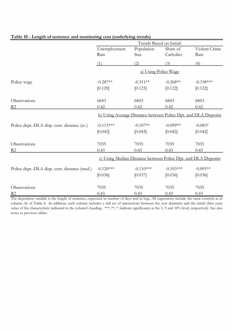
Unemployment

Rate

Population

Size

Share of

Catholics

Violent Crime

Rate

(1) (2) (3) (4)

Police wage -0.287** -0.311** -0.268** -0.338***

[0.120] [0.123] [0.122] [0.122]

Observations 6843 6843 6843 6843

R2 0.42 0.42 0.42 0.42

Police dept.-DLA disp. cent. distance (av.) -0.113*** -0.107** -0.099** -0.083*

[0.042] [0.043] [0.042] [0.042]

Observations 7035 7035 7035 7035

R2 0.43 0.43 0.43 0.43

Police dept.-DLA disp. cent. distance (med.) -0.120*** -0.110*** -0.103*** -0.091**

[0.036] [0.037] [0.036] [0.036]

Observations 7035 7035 7035 7035

R2 0.43 0.43 0.43 0.43

Table 10 - Length of sentence and monitoring cost (underlying trends)

Trends Based on Initial:

The dependent variable is the length of sentence, expressed in number of days and in logs. All regressions include the same controls as in

column (4) of Table 4. In addition, each column includes a full set of interactions between the year dummies and the initial (first year)

value of the characteristic indicated in the column's heading. ***, **, *: indicate significance at the 1, 5 and 10% level, respectively. See also

notes to previous tables.

a) Using Police Wage

b) Using Average Distance between Police Dpt. and DLA Deposits

c) Using Median Distance between Police Dpt. and DLA Deposits

Whole

Sample

All

Sentences

No Large

Sentences

Median

Regression

Off. in State

of Residence

Excl. Alaska

and Hawaii

Excl. Texas

and Virginia

Excl. Maine

and N. Dakota

Excl. Texas

and Florida

Federal

Inmates

State

Inmates

Whole

Sample

Whole

Sample

Whole

Sample

(1) (2) (3) (4) (5) (6) (7) (8) (9) (10) (11) (12) (13) (14)

Death penalty 0.491** 0.470** 0.306** 0.403*** 0.519** 0.494** 0.500** 0.497** 0.491** 0.006 0.624*** 0.253** 0.091***

[0.202] [0.201] [0.155] [0.119] [0.254] [0.202] [0.205] [0.202] [0.205] [0.168] [0.229] [0.123] [0.033]

Republican share 0.241 0.377**

[0.188] [0.184]

Demographic controls yes yes yes yes yes yes yes yes yes yes yes yes yes yes

Criminal record controls yes yes yes yes yes yes yes yes yes yes yes yes yes yes

State controls yes yes yes yes yes yes yes yes yes yes yes yes yes yes

Offense level dummies yes yes yes yes yes yes yes yes yes yes yes yes yes yes

Year dummies yes yes yes yes yes yes yes yes yes yes yes yes yes yes

Observations 7035 7562 6983 7035 5512 6975 5946 7026 5520 1815 5200 7035 7035 7035

R2 0.48 0.47 0.47 0.49 0.48 0.47 0.48 0.47 0.60 0.48 0.42 0.43 0.42

Estimator OLS OLS OLS OLS OLS OLS OLS OLS OLS OLS OLS 2SLS OLS OLS

First-Stage Results

Private wage - - - - - - - - - - - 1.492*** - -

- - - - - - - - - - - [0.095] - -

Kleibergen-Paap F -statistic - - - - - - - - - - - 248.0 - -

Table 11 - Length of sentence and maximum penalty (alternative identification strategies)

b) IV and Reduced-Form Regressionsa) State and Division-Year Fixed Effects

The dependent variable is the length of sentence, expressed in number of days and in logs. Republican share is the share of votes cast for the republican candidate in a given state during the last Presidential election. The regressions in panel a) also include state and Census division-year

fixed effects. ***, **, *: indicate significance at the 1, 5 and 10% level, respectively. See also notes to previous tables.

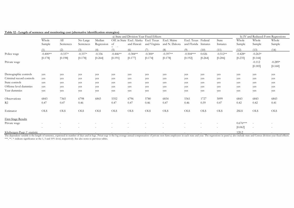
Whole

Sample

All

Sentences

No Large

Sentences

Median

Regression

Off. in State

of

Residence

Excl. Alaska

and Hawaii

Excl. Texas

and Virginia

Excl. Maine

and N. Dakota

Excl. Texas

and Florida

Federal

Inmates

State

Inmates

Whole

Sample

Whole

Sample

Whole

Sample

(1) (2) (3) (4) (5) (6) (7) (8) (9) (10) (11) (12) (13) (14)

Police wage -0.400** -0.337* -0.337* -0.336 -0.446** -0.384** -0.300* -0.397** -0.504*** 0.026 -0.512** -0.428* -0.263*

[0.178] [0.198] [0.178] [0.264] [0.191] [0.177] [0.174] [0.178] [0.192] [0.264] [0.206] [0.235] [0.144]

Private wage -0.112 -0.289*

[0.185] [0.160]

Demographic controls yes yes yes yes yes yes yes yes yes yes yes yes yes yes

Criminal record controls yes yes yes yes yes yes yes yes yes yes yes yes yes yes

State controls yes yes yes yes yes yes yes yes yes yes yes yes yes yes

Offense level dummies yes yes yes yes yes yes yes yes yes yes yes yes yes yes

Year dummies yes yes yes yes yes yes yes yes yes yes yes yes yes yes

Observations 6843 7365 6798 6843 5352 6796 5780 6834 5361 1727 5099 6843 6843 6843

R2 0.47 0.47 0.46 0.47 0.47 0.46 0.47 0.46 0.59 0.47 0.42 0.42 0.41

Estimator OLS OLS OLS OLS OLS OLS OLS OLS OLS OLS OLS 2SLS OLS OLS

First-Stage Results

Private wage - - - - - - - - - - - 0.676*** - -

- - - - - - - - - - - [0.062] - -

Kleibergen-Paap F -statistic - - - - - - - - - - - 120.2 - -The dependent variable is the length of sentence, expressed in number of days and in logs. Private wage is the log average annual compensation of private non-farm employees in each state and year. The regressions in panel a) also include state and Census division-year fixed effects.

***, **, *: indicate significance at the 1, 5 and 10% level, respectively. See also notes to previous tables.

b) IV and Reduced-Form Regressionsa) State and Division-Year Fixed Effects

Table 12 - Length of sentence and monitoring cost (alternative identification strategies)

(1) (2) (3) (4)

Death penalty 0.004*** 0.003**

[0.001] [0.001]

Per capita executions 0.020***

[0.005]

Per prisoner executions 0.008***

[0.002]

State controls no yes yes yes

Observations 1046 647 647 646

R2 0.06 0.26 0.26 0.23

Table 13 - Enforcement and maximum penalty

The dependent variable is the employment share of policemen in each state and year. The sample consists of a

panel of 51 US states between 1982 and 2003. All regressions include year fixed effects. ***, **, *: indicate

significance at the 1, 5 and 10% level, respectively. See also notes to previous tables.

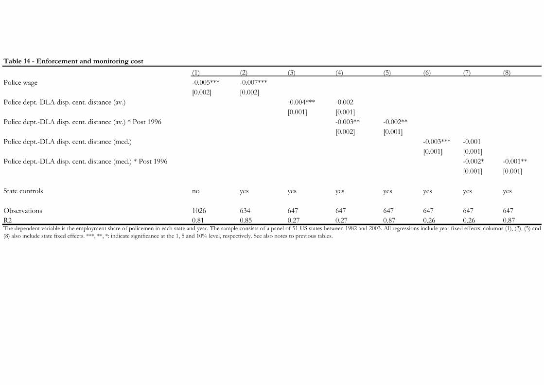
(1) (2) (3) (4) (5) (6) (7) (8)

Police wage -0.005*** -0.007***

[0.002] [0.002]

Police dept.-DLA disp. cent. distance (av.) -0.004*** -0.002

[0.001] [0.001]

Police dept.-DLA disp. cent. distance (av.) * Post 1996 -0.003** -0.002**

[0.002] [0.001]

Police dept.-DLA disp. cent. distance (med.) -0.003*** -0.001

[0.001] [0.001]

Police dept.-DLA disp. cent. distance (med.) * Post 1996 -0.002* -0.001**

[0.001] [0.001]

State controls no yes yes yes yes yes yes yes

Observations 1026 634 647 647 647 647 647 647

R2 0.81 0.85 0.27 0.27 0.87 0.26 0.26 0.87

Table 14 - Enforcement and monitoring cost

The dependent variable is the employment share of policemen in each state and year. The sample consists of a panel of 51 US states between 1982 and 2003. All regressions include year fixed effects; columns (1), (2), (5) and

(8) also include state fixed effects. ***, **, *: indicate significance at the 1, 5 and 10% level, respectively. See also notes to previous tables.

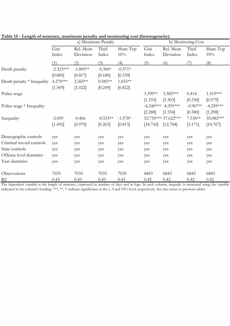
Gini

Index

Rel. Mean

Deviation

Theil

Index

Share Top

10%

Gini

Index

Rel. Mean

Deviation

Theil

Index

Share Top

10%

(1) (2) (3) (4) (5) (6) (7) (8)

Death penalty -2.323*** -1.809** -0.306* -0.571*

[0.885] [0.817] [0.180] [0.339]

Death penalty * Inequality 4.270*** 2.365** 0.585** 1.655**

[1.569] [1.022] [0.249] [0.822]

Police wage 3.399** 3.382*** 0.414 1.519***

[1.355] [1.303] [0.330] [0.579]

Police wage * Inequality -6.240*** -4.395*** -0.907** -4.259***

[2.288] [1.554] [0.380] [1.298]

Inequality -2.059 -0.466 -0.533** -1.578* 52.750*** 37.622*** 7.536** 35.082***

[1.492] [0.970] [0.263] [0.813] [18.742] [12.784] [3.171] [10.767]

Demographic controls yes yes yes yes yes yes yes yes

Criminal record controls yes yes yes yes yes yes yes yes

State controls yes yes yes yes yes yes yes yes

Offense level dummies yes yes yes yes yes yes yes yes

Year dummies yes yes yes yes yes yes yes yes

Observations 7035 7035 7035 7035 6843 6843 6843 6843

R2 0.43 0.43 0.43 0.43 0.42 0.42 0.42 0.42

Table 15 - Length of sentence, maximum penalty and monitoring cost (heterogeneity)

The dependent variable is the length of sentence, expressed in number of days and in logs. In each column, inequality is measured using the variable

indicated in the column's heading. ***, **, *: indicate significance at the 1, 5 and 10% level, respectively. See also notes to previous tables.

a) Maximum Penalty b) Monitoring Cost

Steep

Schedule

Flat

Schedule

Steep

Schedule

Flat

Schedule

Steep

Schedule

Flat

Schedule

Steep

Schedule

Flat

Schedule

(1) (2) (3) (4) (5) (6) (7) (8)

Death penalty 1.057** 0.046

[0.419] [0.068]

Police wage -0.905*** -0.267

[0.270] [0.198]

Schedule slope -0.086** 0.022

[0.031] [0.015]

Schedule slope * Offense level -0.125* 0.017

[0.062] [0.022]

Observations 3,166 3,668 3,105 3,552 20 20 414 413

R2 0.48 0.40 0.47 0.39 0.17 0.06 0.50 0.57

The dependent variables are indicated in the columns' heading, and are: the length of sentence, expressed in number of days and in logs (columns 1-4); the

average offense level of inmates in the state where the offense occurred (columns 5 and 6); and the number of inmates by state and offense level (columns 7 and

8). The regressions in columns (1)-(4) include the same controls as in column (4) of Table 4. The regressions in columns (7) and (8) include state and offense

level fixed effects. Standard errors reported in square brackets are corrected for clustering by state-year in columns (1)-(4), for heteroskedasticity in columns (5)

and (6), and for clustering by state in columns (7) and (8). States with steep (flat) schedules are those for which the estimated slope of the punishment-severity

schedule is above (below) the sample median. ***, **, *: indicate significance at the 1, 5 and 10% level, respectively. See also notes to previous tables.

Table 16 - Additional Evidence on Marginal Deterrence

Dependent Variable:

Sentence Length

Dependent Variable:

Sentence Length

Dependent Variable:

Average Offense Level

Dependent Variable:

Number of Inmates

Figure 1 - Punishment-Severity Schedules

The figure plots the median sentence length across all inmates on the base offense level assigned to

their crime. Figure 1a) reports the unconditional relation whereas Figure 1b) plots the schedule

conditional on individual and state characteristics.

16

11

16

21

26

Length

of S

ente

nce (O

ff.L

ev. 1 =

1)

1 2 3 4 5 6 7 8 9 10 11 12 13 14 15 16 17 18 19 20 21 22 23 24 25 26 27 28 29 30 31 32 33 34 35 36 37 38 39 40 41 42 43

Offense Level

a) Unconditional Schedule

16

11

16

21

26

Length

of S

ente

nce (O

ff.L

ev. 1 =

1)

1 2 3 4 5 6 7 8 9 10 11 12 13 14 15 16 17 18 19 20 21 22 23 24 25 26 27 28 29 30 31 32 33 34 35 36 37 38 39 40 41 42 43

Offense Level

b) Conditional Schedule

Figure 2 - Punishment-Severity Schedules: Distribution of Slope Coefficients across States

The figure plots the distribution of the slopes of state-specific punishment-severity schedules. The

slopes are estimated by running, separately for each state, a regression of log sentence length on

offense level, demographic controls, crime controls, and a time trend. The slope for each state is

the coefficient on offense level from the corresponding regression. Only states with at least 40

inmates are considered.

01

23

45

67

89

10

11

12

Fre

qu

en

cy

-.05 -.04 -.03 -.02 -.01 0 .01 .02 .03 .04 .05Schedule Slope

Figure 3 - Police departments and DLA disposition centers

The figure plots the position of each state police department (red hollow dots) and DLA disposition center (green dots). Data for Alaska and Hawaii are

available to us and used in the regressions, but are not displayed in the figure to make it more readable.

Police Department (6732)DLA Disposition Center (77)