María Padilla-Romo - econstor.eu

econstorMake Your Publications Visible.

A Service of

zbwLeibniz-InformationszentrumWirtschaftLeibniz Information Centrefor Economics

Lindo, Jason M.; Padilla-Romo, María

Working Paper

Kingpin Approaches to Fighting Crime andCommunity Violence: Evidence from Mexico's DrugWar

IZA Discussion Papers, No. 9067

Provided in Cooperation with:IZA – Institute of Labor Economics

Suggested Citation: Lindo, Jason M.; Padilla-Romo, María (2015) : Kingpin Approaches toFighting Crime and Community Violence: Evidence from Mexico's Drug War, IZA DiscussionPapers, No. 9067, Institute for the Study of Labor (IZA), Bonn

This Version is available at:http://hdl.handle.net/10419/111512

Standard-Nutzungsbedingungen:

Die Dokumente auf EconStor dürfen zu eigenen wissenschaftlichenZwecken und zum Privatgebrauch gespeichert und kopiert werden.

Sie dürfen die Dokumente nicht für öffentliche oder kommerzielleZwecke vervielfältigen, öffentlich ausstellen, öffentlich zugänglichmachen, vertreiben oder anderweitig nutzen.

Sofern die Verfasser die Dokumente unter Open-Content-Lizenzen(insbesondere CC-Lizenzen) zur Verfügung gestellt haben sollten,gelten abweichend von diesen Nutzungsbedingungen die in der dortgenannten Lizenz gewährten Nutzungsrechte.

Terms of use:

Documents in EconStor may be saved and copied for yourpersonal and scholarly purposes.

You are not to copy documents for public or commercialpurposes, to exhibit the documents publicly, to make thempublicly available on the internet, or to distribute or otherwiseuse the documents in public.

If the documents have been made available under an OpenContent Licence (especially Creative Commons Licences), youmay exercise further usage rights as specified in the indicatedlicence.

www.econstor.eu

DI

SC

US

SI

ON

P

AP

ER

S

ER

IE

S

Forschungsinstitut zur Zukunft der ArbeitInstitute for the Study of Labor

Kingpin Approaches to Fighting Crime andCommunity Violence:Evidence from Mexico’s Drug War

IZA DP No. 9067

May 2015

Jason M. LindoMaría Padilla-Romo

Kingpin Approaches to Fighting Crime

and Community Violence: Evidence from Mexico’s Drug War

Jason M. Lindo Texas A&M University,

NBER and IZA

María Padilla-Romo Texas A&M University

Discussion Paper No. 9067 May 2015

IZA

P.O. Box 7240 53072 Bonn

Germany

Phone: +49-228-3894-0 Fax: +49-228-3894-180

E-mail: [email protected]

Any opinions expressed here are those of the author(s) and not those of IZA. Research published in this series may include views on policy, but the institute itself takes no institutional policy positions. The IZA research network is committed to the IZA Guiding Principles of Research Integrity. The Institute for the Study of Labor (IZA) in Bonn is a local and virtual international research center and a place of communication between science, politics and business. IZA is an independent nonprofit organization supported by Deutsche Post Foundation. The center is associated with the University of Bonn and offers a stimulating research environment through its international network, workshops and conferences, data service, project support, research visits and doctoral program. IZA engages in (i) original and internationally competitive research in all fields of labor economics, (ii) development of policy concepts, and (iii) dissemination of research results and concepts to the interested public. IZA Discussion Papers often represent preliminary work and are circulated to encourage discussion. Citation of such a paper should account for its provisional character. A revised version may be available directly from the author.

IZA Discussion Paper No. 9067 May 2015

ABSTRACT

Kingpin Approaches to Fighting Crime and Community Violence: Evidence from Mexico’s Drug War*

This study considers the effects of the kingpin strategy, an approach to fighting organized crime in which law-enforcement efforts focus on capturing the leaders of the criminal organization, on community violence in the context of Mexico’s drug war. Newly available historical data on drug-trafficking organizations’ areas of operation at the municipality level and monthly homicide data allow us to control for a rich set of fixed effects and to leverage variation in the timing of kingpin captures to estimate their effects. This analysis indicates that kingpin captures have large and sustained effects on the homicide rate in the municipality of capture and smaller but significant effects on other municipalities where the kingpin’s organization has a presence, supporting the notion that removing kingpins can have destabilizing effects throughout an organization that are accompanied by escalations in violence. JEL Classification: I18, K42, O12 Keywords: violence, crime, kingpin, Mexico, drugs, cartels Corresponding author: Jason M. Lindo Texas A&M University Department of Economics 4228 TAMU College Station, TX 77843 USA E-mail: [email protected]

* Padilla-Romo gratefully acknowledges support from the Private Enterprise Research Center at Texas A&M University.

mailto:[email protected]

1 Introduction

The two main reasons for waging war on drugs are to reduce societal costs associated with

drug abuse and to reduce societal costs associated with the drug trade. The former includes

effects on health, productivity, violent behavior, and broader impacts on health care and

public assistance programs. The latter includes violence involved with the enforcement of

contracts and turf battles, corruption, and activity in related “industries” that are detri-

mental to welfare including protection rackets, human smuggling, kidnapping, prostitution,

weapons trafficking, theft, etc.1 Naturally, the relative importance of these costs depends

on many factors, including the types of drugs involved, the level and spatial distribution of

demand, and the organization of the supply network.2 Correspondingly, there is significant

heterogeneity in the approaches that have been used to wage war on drugs. Demand-side

approaches take the form of prevention efforts, treatment for abusers, and increases in the

cost of abuse through enforcement efforts and punishment. Supply-side approaches, on the

other hand, focus on disrupting operations by way of confiscation of drugs and guns, target-

ing precursors, and arresting and punishing those involved in the drug trade. Given resource

constraints, policy-makers have to consider which of these policies to use and how intensely

to use them, highlighting the importance of understanding their costs and benefits. Towards

this end, this paper considers the effects of a particular supply-side approach that has played

a prominent role in Mexico’s drug war—the targeting of high-ranked members of criminal

organizations, also known as the “kingpin strategy”—on community violence.

To put this study into context, it is important to note that most of the existing research

in this area focuses on the effects of drug-related interventions on drug abuse in “downstream

markets.” For example, researchers have shown that the Taliban stamping out poppy pro-

duction reduced heroin use in Australia (Weatherburn et al. 2003), that the effects of Plan

Colombia on the supply of Cocaine to the US were relatively small (Mejıa and Restrepo

2013), that reductions in methamphetamine availability in the United States in the mid-1990s

reduced drug-related harms (Cunningham and Liu 2003; Dobkin and Nicosia 2009; Cunning-

1Drug-related violence additionally appears to have detrimental effects on economic activity as measuredby labor force participation and unemployment rates (Robles, Calderon, and Magaloni 2013).

2For example, the societal costs associated with the drug trade are most important in areas heavilyinvolved in the illegal production and distribution of drugs to be consumed elsewhere.

2

ham and Finlay 2013), that US state laws limiting the availability of Pseudoephedrine have

not changed methamphetamine consumption (Dobkin, Nicosia, and Weinberg 2013) nor have

graphic advertising campaigns (Anderson 2010), and that substance-abuse treatment avail-

ability reduces mortality (Swensen forthcoming). In contrast, relatively little is known about

the causal effects of “upstream interventions” on “upstream communities,” i.e., the effects

of interventions on outcomes in areas where production, distribution, and their associated

costs are most relevant. The two studies that speak most directly to this specific issue

are Angrist and Kugler (2008), which shows that exogenous shocks to coca prices increase

violence in rural Colombian districts as groups fight over additional rents and Dell (2014),

which shows that drug-trade crackdowns in Mexico driven by PAN mayoral victories increase

drug-trade-related homicides.3

This paper contributes to this literature by considering the effects of the kingpin strategy,

which has featured prominently in Mexico’s war on drugs. Proponents of the kingpin strategy

argue that removing a leader weakens an organization through its effect on its connections,

its reputation, and by creating disarray in the ranks below, and that this may in turn reduce

the organization’s level of criminal activity. Detractors, however, point out that this strategy

may increase violence as lower ranked members maneuver to succeed the eliminated leader

and rival groups attempt to exploit the weakened state of the organization. Given sound

logic underlying arguments in favor of and against the kingpin strategy, there is a clear need

for empirical research on the subject. That said, there are two main empirical challenges to

estimating the effect of the kingpin strategy that are difficult to overcome. First, policies

targeting organized crime are almost always multifaceted, involving the simultaneous use of

various strategies. Mexico’s war on drugs is no exception—it also involved various approaches

implemented at various times with varying degrees of intensity, which we discuss in greater

detail in the next section. The second main challenge is that the capture of a kingpin is fairly

rare because, by definition, they are small in number. As a result, establishing compelling

evidence on the effect of eliminating kingpins in some sense requires a series of case studies.

This study attempts to overcome these challenges by exploiting variation in the timing with

3In related work, Mejıa and Restrepo (2013) estimate the causal effect of the drug trade on violence usingvariation in the prominence of the drug-trade in Colombian municipalities based on land suitability for cocacultivation.

3

which different Mexican DTOs had their leaders captured during Mexico’s drug war and by

using detailed data on the geographic distribution of DTOs over time (based on Coscia and

Rios (2012)) to form different comparison groups. This approach allows us to abstract away

from the effects of broader policies and shocks (at the national and/or state level) and to

conduct several ancillary analyses to guide our interpretation of the results.

We find that the capture of a DTO leader in a municipality increases its homicide rate

by 80% and that this effect persists for at least twelve months. Consistent with the notion

that the kingpin strategy causes widespread destabilization throughout an organization, we

also find significant effects on other municipalities with the same DTO presence. In partic-

ular, we find a significant short-run effect (30% 0–6 months after capture) that dissipates

over time for neighboring municipalities with the same DTO presence and an effect that is

immediately small but grows over time (18% 12+ months after capture) for more-distant mu-

nicipalities with the same DTO presence. We find little evidence of any effect on neighboring

municipalities where the captured leader’s DTO did not have a presence.

Several additional pieces of evidence support a causal interpretation of these main results.

First, there is no indication that homicides deviate from their expected levels prior to a

kingpin’s capture, suggesting that the main results are not driven by the sorts of efforts that

might precede a capture such as the mobilization of troops into an area. We also show that

the main results are driven by effects on the individuals most likely to be directly involved

in the drug trade: males and, more specifically, working-age males. In an additional effort

to show that the main results are not simply reflecting an increase in propensities to engage

in violence that coincides with captures in the relevant municipalities, we demonstrate that

domestic violence and infant mortality do not respond to these events. Lastly, we present

evidence that operations themselves do not increase homicides in an analysis of the first

major operations of the war on drugs.

The remainder of the paper is organized as follows. In the next section, we provide

background on Mexico’s drug war, including a discussion of the events that precipitated it,

and the relevant DTOs. We then discuss our data and empirical strategy in sections 3 and

4, respectively. Section 5 presents a graphical analysis, the main results, and supporting

analyses. Lastly, Section 6 discusses the results and concludes.

4

2 Background

2.1 Drug-trafficking in Mexico

In many ways, Mexico is ideally situated for producing and trafficking drugs. In addition

to having a climate that allows for the growth of a diverse set of drugs, it shares a border

with the world’s biggest consumer of drugs, the United States. Drug trafficking has also

been able to flourish in Mexico as a result of corruption and weak law enforcement. The first

DTOs were protected by the government, which designated the areas in which each DTO

would carry out their illegal activities. In the 1980s, former police officer Miguel Angel Felix

Gallardo—together with Rafael Caro Quintero and Ernesto Fonseca Carrillo—founded the

first Mexican Cartel: the Guadalajara Cartel.4 After the incarceration of his partners in 1985,

Felix Gallardo kept a low profile and decided to divide up the areas in which he operated.5

According to Grayson (2014), the government and the DTOs had unwritten agreements

that “DTO leaders respected the territories of competitors and had to obtain crossing rights

before traversing their turfs...criminal organization[s] did not sell drugs in Mexico, least of

all to children...and prosecutors and judges would turn a blind eye to cooperative criminals.”

In the 1990s, however, the environment became less stable as Guadalajara’s DTO splin-

tered into four separate DTOs6 and the Institutional Revolutionary Party (PRI) lost political

power (Astorga and Shirk 2010). Morales (2011) describes the late 1990s and early 2000s

as a period in which the DTOs became more independent, going from a regimen of political

subordination to one of direct confrontation to dispute the control of territory. In late 2005,

a new DTO—La Familia—was established in the state of Michoacan followed by a wave of

violence.7 At the beginning of the war on drugs there were five DTOs (or alliances of DTOs),

Sinaloa/Beltran-Leyva, Gulf, Tijuana, La Familia, and Juarez.

4In addition with his connections with the Mexican government, Felix Gallardo was the first Mexicandrug trafficker to make connections with Colombian cartels, particularly he established a solid relation withPablo Escobar (leader of the Medellın Cartel).

5Joaquın Guzman Loera and Ismael Zambada Garcıa were given the pacific coast area, the Arellano Felixbrothers received the Tijuana corridor, the Carrillo Fuentes family got the Ciudad Juarez corridor, and JuanGarcıa Abrejo received the Matamoros corridor.

6After the arrest of Felix Gallardo in 1989 and his transfer to a the maximum security prison La Palmain Mexico state, the leaders of the designated areas became independent and founded the second generationof cartels (Sinaloa, Tijuana, Juarez, and Gulf).

7La Familia DTO is the metamorphosis of La Empresa which was a former branch of the Gulf Cartel.

5

2.2 The War on Drugs

As shown in Panel A of Figure 1, the homicide rate in Michoacan grew dramatically between

2005 and 2006. That said, the national homicide rate continued to be extremely stable at

0.8 per 100,000 residents per month (Figure 1, Panel B). Nonetheless, eleven days after

the beginning of his term, the newly elected President Felipe Calderon declared war on the

DTOs on December 11, 2006, citing the increase in violence in Michoacan as the last straw.

While pundits highlighted his desire to have significant reform associated with his presidency

and the fact that he was born and raised in Michoacan, his stated reasons for initiating the

war was a concern “about the growth of drugs-related violence and the existence of criminal

groups trying to take over control of entire regions.”8 Calderon’s strategy mainly consisted

in a frontal attack led by members of the army, the navy, and the federal police seeking

the eradication of crops, the confiscation of drugs and guns, and the incarceration or killing

of high ranked drug traffickers (the kingpin strategy). The first operation took place in

Michoacan on December 11, 2006, where more than 5000 army and federal police elements

were deployed, and subsequent operations followed in other parts of the country.

Mexico’s war on drugs was initially viewed as a great success. As shown in Figure 2,

plotting data from 2001 to 2010, the national homicide rate dropped sharply in January

2007. The homicide rate jumped back up to 0.72 in March—not quite to its earlier level—

and then held steady for the following 9 months. Then, at the beginning of 2008 in a clear

break from trend, the homicide rate started to climb. It would continue to climb for several

years, reaching a level 150% higher than the pre-drug-war rate at the end of 2010.

This dramatic increase in violence in Mexico has drawn the attention of researchers from

different disciplines trying to explain its causes—most attribute this increase in violence to

Calderon’s war on drugs. Different researchers have focused on the role of the deployment

of federal troops all across the country (Escalante 2011, Merino 2011), the expiration of the

U. S. Federal Assault Weapons Ban in 2004 (Chicoine 2011, Dube et. al. 2012), the increase

of cocaine seizures in Colombia (Castillo et al. 2012, Mejıa 2013), and the increased effort

to enforce law initiated by the National Action Party (PAN) mayors (Dell, 2011).

Our research is motivated by the observation that the escalation of violence began in

8Financial Times interview, conducted January 17, 2007.

6

January 2008, which was the month in which the first cartel leader was captured during

the war on drugs (Alfredo Beltran Leyva). Naturally, many other things were going on in

Mexico and around the world at the same time, necessitating a more rigorous consideration

to be able to draw any strong conclusions about the effects of Mexico’s kingpin strategy. In

order to conduct such an analysis, we make use of newly available data on the geographic

distribution of DTOs over time—in conjunction with several other data sets—to consider the

first captures of kingpins associated with each of the five DTOs in operation at the beginning

of the war on drugs. These data and the associated identification strategy are described in

the next sections.

3 Data

Our analysis brings together data from several sources that ultimately yields a data set at

the municipality-month level, spanning January 2001 through December 2010. Our primary

outcome variable is based on monthly homicides at the municipality level, constructed using

the universe of death certificates from the vital statistics of the National Institute of Statistics

and Geography (INEGI).9 In order to put these data into per capita rates, we use estimated

municipality population counts from the National Council of Population (CONAPO) and El

Colegio de Mexico (COLMEX), which are based on projections from the Census of Population

and Housing. While we note that drug-related homicides are available from December 2006

to October 2011, we do not use these data out of concern for the endogeneity of homicides

being classified as “drug related” or “not drug related.”

Our information on kingpin captures are from a compendium of press releases of the

Army (SEDENA), the Navy (SEMAR), and the Office of the Attorney General (PGR).

While these press releases contain a wealth of additional information, we focus on the timing

of the first capture of a leader or lieutenant from each of the DTOs during the war on drugs.

To put into perspective the types of kingpins we are considering, as the name implies, leaders

are at the very highest level of the DTO organization. Lieutenants are immediately below

9Less than one percent of death certificates with homicide as the presumed cause of death are missingthe municipality of occurrence. These observations are not used in our analysis.

7

leaders in the DTO organization. As a practical matter, we classify an event as a capture

of a DTO leader when a press release indicates that the individual was a head (or one of

the heads) of a DTO and identify an event as a capture of a DTO lieutenant when a press

release indicates that the individual was a leader of a DTO in some state or region. We do

not consider events in which the press release indicates that the individual was a leader only

in a particular municipality, indicating that the individual was likely a plaza boss.

As shown in Table 1, there is significant variation in the timing with which high-level

kingpins were captured for the five DTOs in operation at the beginning of the war on drugs.

The first took place on August 29th, 2007—eight months after the war on drugs began—

when Juan Carlos de la Cruz Reyna, a lieutenant in the Gulf Cartel was captured. The first

other four DTOs (Sinaloa-Beltran-Leyva, Tijuana, Juarez, and La Familia) had top level

leaders captured at various times between January and December of 2008.10

We use newly available historical data on the municipalities of operation for each DTO,

the construction of which is described in detail in Coscia and Rios (2012). Briefly, the data

was constructed using a MOGO (Making Order using Google as an Oracle) framework for

selecting the most reliable subset of web information to collect information on relationships

between sets of entities (DTOs and municipalities in this case). It uses indexed web content

(e.g., online newspapers and blogs) and various queries to identify DTOs’ areas of operation

at the municipality level between 1990 and 2010.11 To avoid concerns about endogeneity,

we define areas of operation using only data before the war on drugs began (2001-2006).

Moreover, we take a conservative approach and specify that a DTO had a presence in a

municipality if the municipality was an “area of operation” for the DTO in any of these five

years. Figure 3 maps out the distribution of the of the DTOs based on this definition. One

important takeaway from this figure—which we exploit in our empirical analysis—is that a

large share of Mexico has no DTO presence (or a DTO presence that is too weak or inactive

to be picked up using Coscia and Rios’ approach).

10Sinaloa and Beltran-Leyva DTOs were allied before the drug war commenced.11Such data was previously only available to the research community at the state level.

8

4 Empirical Strategy

While we begin our analysis of the effects of the kingpin captures homicides with a series of

graphical comparisons, our main results are based on a generalized difference-in-difference

approach. In particular, we estimate the effects of kingpin captures using the following

regression model:

lnHmt = Dmtδ + αm + γt +Xmtβ + umt (1)

where lnHmt is the natural log of the homicide rate in municipality m at time t; Dmt is a

set of indicator variables reflecting whether a kingpin relevant to the municipality has been

captured in 0–5 months ago, 6–11 months ago, or 12+ months ago; αm are municipality

fixed effects; γt are month-by-year fixed effects; Xmt can include time-varying municipality

controls; and umt is an error term.12 As such, the estimates are identified by comparing

changes in violence among affected and non-affected municipalities using variation in the

timing with which different municipalities are affected because of their links to different

DTOs (and having no link to any DTO). This approach allows us to avoid biases that

would otherwise be introduced by fixed differences across municipalities and by the effects

of any shocks or interventions that are common across municipalities. The fact that we

have municipalities associated with different DTOs who have kingpins captured at different

times and we also have municipalities without any DTO presence allows us to additionally

control for the effects of the war on drugs that are common to municipalities with a DTO

presence, which we accomplish by including variables for 0–5, 6–11, and 12+ months after

the beginning of the war interacted with an indicator for the presence of a DTO in the

municipality. We can also control for additional spatial heterogeneity by including state-by-

year fixed effects in the model.

Two main aspects of the empirical analysis that we have yet to discuss in detail are:

how to define whether a kingpin capture is “relevant to a municipality” and what sorts of

captures are considered. We define a kingpin capture as being “relevant to a municipality”

in four different ways to allow for treatment effect heterogeneity. In particular, we separately

estimate effects of a kingpin capture on the municipality of capture, neighboring municipal-

12We add one to the homicide count to avoid missing values.

9

ities where the captured kingpin’s DTO had a presence, other neighboring municipalities,

and non-neighboring municipalities where the captured kingpin’s DTO had a presence. As

described in the previous section, our analysis of “kingpins” focuses DTO leaders and lieu-

tenants, i.e., those at the very top level of the organization and those who control a state or

region. We further restrict attention to the first capture of a kingpin for each DTO during

the war on drugs. We do so out of concern for the endogeneity that would be introduced

when the capture of a kingpin affects the outcome while also increasing the probability of

the capture of subsequent kingpins. By focusing instead on the effects of an initial capture,

our estimates will reflect the effect of a kingpin capture on outcomes that is inclusive of the

effects driven by subsequent captures.

We note that standard-error estimation is not straightforward in this context. While

we are evaluating a panel of municipalities, there may be reason to cluster standard-error

estimates at some higher level(s) because different municipalities may have correlated shocks

to outcomes not captured by our model. In some sense, because the source of variation is at

the DTO level, it may be preferable to allow the errors to be correlated across municipalities

when they share the presence of the same DTO. However, with only five DTOs, this would

lead to problems associated with too few clusters. As a compromise, we instead cluster on

DTO-combinations, which leverages the fact that there are some municipalities where two

or three municipalities have a presence.13 We additionally cluster on states to allow for some

spatial correlation in the errors that might occur naturally or through policies implemented

at the state level, following the approach to multi-way clustering described in Cameron,

Gelbach, and Miller (2011).14

132,224 municipalities have no DTO presence, 181 have one, 43 have two, and only six have three.14This approach leads to somewhat more conservative standard-error estimates than clustering only on

states, only on DTO combinations, or only on municipalities.

10

5 Results

5.1 Graphical Evidence of the Effects of Kingpin Captures

Before presenting the results of the econometric analysis described above, in this section we

present graphical evidence. To begin, Figure 4 plots the homicide rate over time separately

for counties with a DTO presence before the war on drugs and those that did not have such

a presence. This figure shows that municipalities with a DTO presence had higher—but not

much higher—homicide rates than municipalities without a DTO presence in the six years

leading up to the war on drugs. Moreover, they tracked one another quite closely. Perhaps

most importantly, they even tracked one another after the beginning of the war on drugs—

both dipping immediately before returning to close to their earlier levels—which provides

support for using municipalities without a DTO presence as a meaningful comparison group

for the purpose of attempting to separate the effects of kingpin captures from the effects

of other aspects of the war on drugs. Twelve months after the beginning of the war on

drugs, however, the two series began to diverge from one another in a dramatic way. While

the capture of Alfredo Beltran Leyva, leader of the Beltran Leyva Cartel, would appear to

be the most salient event to happen around this time that would disproportionately affect

municipalities with a DTO presence, we cannot rule out other explanations such as a lagged

effect of earlier aspects of the war on drugs. One explanation that we can rule out is that the

war on drugs did not begin in earnest until this time—several major operations took place

in 2007 which lead to the seizure of 48,042 Kg of cocaine, 2,213,427 Kg of marijuana, and

317 Kg of heroin, significantly more than the amounts seized in the subsequent years.15

Across the five panels of Figure 5, we take a more systematic look at how homicide rates

changed over time in municipalities with a DTO presence relative to those without in relation

to kingpin captures. In panels A and B, we plot time series that focus on municipalities with

the presence of DTOs whose first captured “kingpin” was a leader at the highest level of the

organization. In particular, in Panel A we plot the homicide rate over time for municipalities

where Sinaloa or Beltran Leyva (allies) had a presence prior to the war on drugs in addition to

the homicide rate for municipalities with no DTO presence for comparison. Consistent with

15Third Calderon’s Government Report (Tercer Informe de Gobierno, 2009).

11

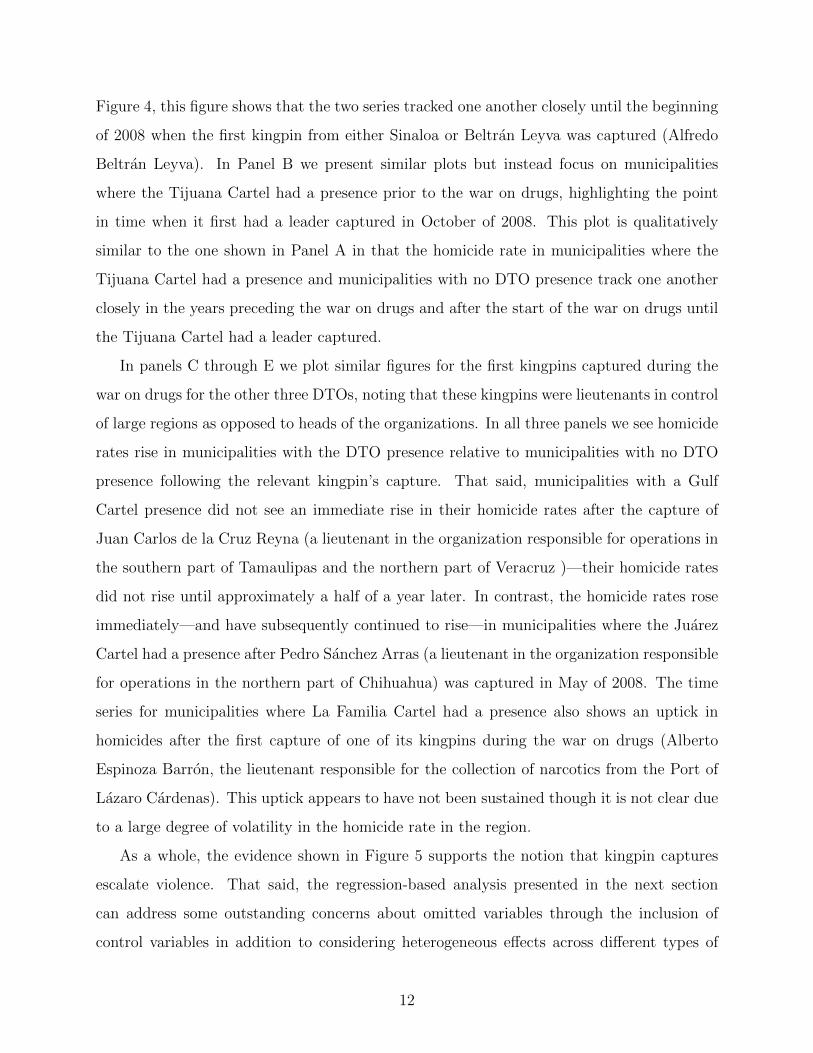
Figure 4, this figure shows that the two series tracked one another closely until the beginning

of 2008 when the first kingpin from either Sinaloa or Beltran Leyva was captured (Alfredo

Beltran Leyva). In Panel B we present similar plots but instead focus on municipalities

where the Tijuana Cartel had a presence prior to the war on drugs, highlighting the point

in time when it first had a leader captured in October of 2008. This plot is qualitatively

similar to the one shown in Panel A in that the homicide rate in municipalities where the

Tijuana Cartel had a presence and municipalities with no DTO presence track one another

closely in the years preceding the war on drugs and after the start of the war on drugs until

the Tijuana Cartel had a leader captured.

In panels C through E we plot similar figures for the first kingpins captured during the

war on drugs for the other three DTOs, noting that these kingpins were lieutenants in control

of large regions as opposed to heads of the organizations. In all three panels we see homicide

rates rise in municipalities with the DTO presence relative to municipalities with no DTO

presence following the relevant kingpin’s capture. That said, municipalities with a Gulf

Cartel presence did not see an immediate rise in their homicide rates after the capture of

Juan Carlos de la Cruz Reyna (a lieutenant in the organization responsible for operations in

the southern part of Tamaulipas and the northern part of Veracruz )—their homicide rates

did not rise until approximately a half of a year later. In contrast, the homicide rates rose

immediately—and have subsequently continued to rise—in municipalities where the Juarez

Cartel had a presence after Pedro Sanchez Arras (a lieutenant in the organization responsible

for operations in the northern part of Chihuahua) was captured in May of 2008. The time

series for municipalities where La Familia Cartel had a presence also shows an uptick in

homicides after the first capture of one of its kingpins during the war on drugs (Alberto

Espinoza Barron, the lieutenant responsible for the collection of narcotics from the Port of

Lazaro Cardenas). This uptick appears to have not been sustained though it is not clear due

to a large degree of volatility in the homicide rate in the region.

As a whole, the evidence shown in Figure 5 supports the notion that kingpin captures

escalate violence. That said, the regression-based analysis presented in the next section

can address some outstanding concerns about omitted variables through the inclusion of

control variables in addition to considering heterogeneous effects across different types of

12

municipalities.

5.2 Regression-based Evidence of the Effects of Kingpin Captures

Columns 1 through 3 of Table 2 present our main results, based on the generalized difference-

in-difference model represented by Equation 1. In particular, these columns show the es-

timated effects of a kingpin capture over time for a municipality of capture, municipalities

where a captured kingpin’s DTO had a presence that do not neighbor the municipality of

capture, neighboring municipalities where a captured kingpin’s DTO had a presence, and

other municipalities neighboring the municipality of capture. The estimates are based on

models that control for municipality fixed effects and month-by-year fixed effects. Column

2 additionally controls for state-by-year fixed effects to address concerns that captures may

be correlated with other state-level policy initiatives and/or shocks while Column 3 further

adds controls for the effects of the war on drugs that are common to municipalities with a

DTO presence by including variables for 0–5, 6–11, and 12+ months after the beginning of

the war interacted with an indicator for the presence of a DTO in the municipality.

Across these columns, we note that the estimates are somewhat sensitive to the inclusion

of state-by-year fixed effects but not to the inclusion controls for the effects of the war on

drugs that are common to municipalities with a DTO presence. Regardless of the exact

specification, the estimates indicate significant effects and considerable heterogeneity. In

particular, the estimates reflect an immediate and sustained effect of a kingpin capture on

the homicide rate in the municipality of capture of approximately 60–80%.16 Consistent with

the notion that the kingpin strategy causes widespread destabilization throughout an organi-

zation, our preferred estimates (Column 3) suggest significant short-run effects on homicide

rates in municipalities where the captured kingpin’s DTO had a presence that neighbored

the municipality of capture: 28% 0–5 months after the capture and 17% 6–11 months after

capture. These estimates are relatively imprecise due to the limited number of municipalities

contributing to the estimates, however, and they are only statistically significant at the 10-

percent level. In contrast, the estimated effects on non-neighboring municipalities where the

16As the outcome is the log of the homicide rate, the percent effects are calculated by exponentiating thecoefficient estimate—in this case 0.48 and 0.58—and subtracting one.

13

captured kingpin’s DTO had a presence are relatively precise, indicating a significant effect

in the short-run (7% 0–5 months following a capture) that appears to grow over time (9%

6–11 months following a capture and 18% 12+ months following a capture). The estimated

effects on municipalities neighboring the municipality of a kingpin capture who do not share

the same DTO presence are routinely negative, suggesting that kingpin captures may lead

to a spatial displacement of violence; however, these estimates tend to not be statistically

significant.

Columns 4 and 5 of Table 2 assess the validity of the research design by considering

whether homicide rates deviate from their expected levels prior to a kingpin capture in any

of these types of municipalities. These estimates are routinely close to zero and are never

statistically significant, which provides support for a causal interpretation of the estimates

discussed above.

5.3 Further Analyses Supporting a Causal Interpretation of the

Main Results

Similar to our analysis verifying that there are no “effects” before a kingpin capture occurs,

which would otherwise suggest that our regression model is picking up something other than

the effects of kingpin captures, in Table 3 we separately consider the estimated effects on

male homicide rates, female homicide rates, rates of domestic violence, and infant mortality

using our preferred model.17 These estimates provide further support for a causal interpre-

tation of our main results: they indicate that the effects are larger for males than females,

which is consistent with gender differences in participation in the drug trade; no effects on

domestic violence, which provides reassuring evidence that the main results are not driven

by idiosyncratic shocks to levels of violence coinciding with kingpin captures; and no effects

on infant mortality, which provides reassuring evidence that the main results are not driven

by compositional changes towards a higher-risk population in the affected municipalities.

Table 4 presents evidence along similar lines, considering effects on homicide rates for

17Domestic violence data comes from administrative records of individuals arrested for the crime of do-mestic violence from Estadsticas Judiciales en Material Penal de INEGI. Infant mortality data is based onthe same source as the homicide data described above.

14

males of different age groups. These estimates indicate that the effects on males are driven

by those between the ages of 15 and 59, mirroring participation rates in drug trafficking

(Fairlie 2002, Vilalta and Martınez 2012). Moreover, the estimated effects on homicides

rates for younger and older males tend to be close to zero and are not statistically significant

any more than we would expect by random chance.

Though our main results are able to control for national and state-level policies and

shocks common across areas in addition those common to municipalities with a DTO presence

through the inclusion of fixed effects, a potential concern with the empirical strategy is that

it might conflate the effects of kingpin captures with the effects of military operations more

broadly. In order to speak to this possibility, Figure 6 considers each of the nine major state

(or multi-state) operations of the war on drugs in the timeframe spanned by our data.18

In particular, each panel restricts attention to the state(s) of the operation and separately

plots the homicide rate for municipalities with and without a DTO presence. Collectively,

these nine panels indicate that the major operations of the drug war did not precipitate

increases in homicides. The one panel (h) that does show a major uptick in homicides at

the beginning of the operation is one in which a kingpin was captured soon after its start19

and the location of the next phase of Sierra Madre operation.20

Figure 7 also focuses on homicide rates as they relate to major operations of the war on

drugs but instead considers municipality-level operations. Notably, all municipalities that

were the target of an operation, saw dramatic rises in their homicide rates. That said, as

with the state level operations, there appears to be no consistent link between operations

of the war on drugs and these rises—some of these municipalities saw their homicide rates

begin to rise before an operation, some after, and some at around the same time.

Table 5 offers an additional check on the main results by considering the sensitivity of the

estimates to the exclusion of considering any given DTO. In particular, across the columns

of the table we report results systematically excluding from the analysis municipalities where

18The beginning dates for these operations are based on information from the fifth Calderons GovernmentReport (Quinto Informe de Gobierno, 2011). End dates are not specified except for Sierra Madre, Marlın,and Culiacan operations.

19Pedro Sanchez Arras, lieutenant in the Juarez Cartel, captured approximately six weeks after the Chi-huahua Operation began.

20Sierra Madre operation was launched on January 7, 2007 in the states of Chihuahua, Durango, andSinaloa.

15

the Sinaloa-Beltran-Leyva cartels have a presence (Column 2), where the Tijuana Cartel has

a presence (Column 3), where the Gulf Cartel has a presence (Column 4), where the Juarez

Cartel has a presence (Column 5), and where the Familia Cartel has a presence (Column 6),

respectively. This analysis is motivated by the notion that we should be less confident in the

results if they are driven by any one particular kingpin’s capture. The estimates are most

sensitive to the exclusion of municipalities where the Sinaloa-Beltran-Leyva and Gulf cartels

have a presence, which span the most municipalities and the municipalities with the largest

populations (as shown in Table 1). That said, the estimates guide us to the same conclusion

regardless of whether any one DTO is not considered in the analysis—kingpin captures have

large and immediate effects on the municipality of capture that are quite persistent; there are

spillover effects onto other municipalities where the captured kingpin’s DTO has a presence;

and there are perhaps some effects on neighboring municipalities where the kingpin’s DTO

does not have a presence.

6 Discussion and Conclusion

In the preceding sections, we have estimated the effects of the first kingpin captures during

Mexico’s war on drugs for the DTOs that were in operation prior to the war. Newly available

data on DTOs’ areas of operation at the municipality level over time and monthly data on

homicides allow us to control for a rich set of fixed effects and to leverage variation in the

timing of kingpin captures to consider the effects on homicides in the area of capture itself in

addition to other areas where the kingpin’s DTO has a presence. The results of this analysis

indicate that kingpin captures have large and sustained effects on the homicide rate in the

municipality of capture and smaller but significant effects on other municipalities where the

kingpin’s DTO has a presence, supporting the notion that the kingpin strategy can have

destabilizing effects throughout an organization while highlighting that this does not imply

a reduction in violence. Spillover effects onto municipalities neighboring the municipality

of capture appear to be small and, if anything, positive (as they suggest a reduction in

homicides).

These estimates offer a new lens through which we can view the dramatic increase in

16

violence in Mexico since the beginning of the war on drugs. In particular, our estimates

suggest that the kingpin captures we consider lead to an additional 11,626 homicides since

2007, or approximately 17 percent of the homicides since that time. Moreover, the effects

of these kingpin captures can explain 36 percent of the 130 percent increase in the homi-

cide rate (or approximately a quarter) between 2006 and 2010.21 An important caveat to

these figures is that we use an imperfect measure of DTOs’ areas of operation (based on the

MOGO approach described above) and that misclassification would serve to bias our esti-

mates towards zero—as such, they may be best thought of as estimates of the lower bound

of the true effects.

While our estimates indicate that Mexico’s use of the kingpin strategy caused significant

increases homicides, it is important to note that its war on drugs had several objectives

beyond reducing violence, including the establishing the rule of law, that need to be consid-

ered in evaluating the policy. Moreover, it remains possible that the kingpin strategy could

reduce violence in the long-run in ways that have yet to be seen.

21These numbers were calculated using the regression coefficients from Column 3 of Table 2. In particular,they are based on the municipalities affected by the capture of a kingpin, multiplying its homicide rate priorto the capture by the relevant coefficient estimate for each year and adjusting for the change in its population.These calculations indicate that the capture of kingpins caused an increase in homicides of approximately600 in 2007, 3,000 in 2008, 3,900 in 2009 and 4100 in 2010.

17

References

Anderson, D. M. (2010): “Does Information Matter? The Effect of the Meth Project onMeth Use among Youths,” Journal of Health Economics, 29, 732–742.

Angrist, J. D., and A. D. Kugler (2008): “Rural windfall or a new resource curse?Coca, income, and civil conflict in Colombia,” Review of Economics and Statistics, 90(2),191–215.

Astorga, L., and D. A. Shirk (2010): “Drug trafficking organizations and counter-drugstrategies in the US-Mexican context,” Center for US-Mexican Studies.

Cameron, A. C., J. B. Gelbach, and D. L. Miller (2011): “Robust Inference WithMultiway Clustering,” Journal of Business and Economic Statistics, 29(2), 238–249.

Castillo, J. C., D. Mejıa, and P. Restrepo (2012): “Illegal drug markets and violencein Mexico: The causes beyond Calderon,” Working Paper.

Chicoine, L. (2011): “Exporting the Second Amendment: U.S. Assault Weapons and theHomicide Rate in Mexico,” Working Paper.

Coscia, M., and V. Rios (2012): “Knowing where and how criminal organizations operateusing web content,” CIKM, pp. 1412–1421.

Cunningham, J. K., and L. M. Liu (2003): “Impacts of federal ephedrine and pseu-doephedrine regulations on methamphetamine-related hospital admissions,” Addiction,98(9), 1229–1237.

Cunningham, S., and K. Finlay (2013): “Parental substance use and foster care: Evi-dence from two methamphetamine supply shocks,” Economic Inquiry, 51(1), 764–782.

Dell, M. (Forthcoming): “Trafficking Networks and the Mexican Drug War,” AmericanEconomic Review.

Dobkin, C., and N. Nicosia (2009): “The war on drugs: methamphetamine, publichealth, and crime,” American Economic Review, 99(1), 324–349.

Dobkin, C., N. Nicosia, and M. Weinberg (2014): “Are supply-side drug control effortseffective? Evaluating OTC regulations targeting methamphetamine precursors.,” Journalof Public Economics, 120, 46–61.

Dube, A., O. Dube, and O. Garcıa-Ponce (2013): “Cross-Border Spillover: U.S. GunLaws and Violence in Mexico,” American Political Science Review, 107(3), 397–417.

Escalante, F. (2011): “Homicidios 2008-2009 La muerte tiene permiso,” Nexos.

Fairlie, R. W. (2002): “Drug Dealing and Legitimate Self-Employment,” Journal of LaborEconomics, 20(3), 538–537.

18

Grayson, G. W. (2013): The Cartels: The Story of Mexico’s Most Dangerous CriminalOrganizations and Their Impact on US Security. ABC-CLIO, Santa Barbara, CA.

Mejıa, D., and P. Restrepo (2013): “Bushes and Bullets: Illegal Cocaine Markets andViolence in Colombia,” Documento CEDE.

Merino, J. (2011): “Los operativos conjuntos y la tasa de homicidios: una medicin,” Nexos.

Morales-Oyarvide, C. (2011): “La Guerra Contra el Narcotrafico en Mexico. Debilidaddel Estado, Orden Local y Fracaso de una Estrategia,” Aposta, 50.

Robles, G., G. Calderon, and B. Magaloni (2013): “Economic Consequences ofDrug-Trafficking Violence in Mexico,” Inter-American Development Bank Working Paper426.

Swensen, I. D. (2015): “Substance-Abuse Treatment and Mortality,” Journal of PublicEconomics, 122, 13–30.

Vilalta, C. J., and J. M. Martinez (2012): “The making of Narco bosses: hard drugdealing crimes among Mexican students,” Trends in organized crime, 15(1), 47–63.

Weatherburn, D., C. Jones, K. Freeman, and T. Makkai. (2003): “Supply controland harm reduction: lessons from the Australian heroin drought,” Addiction, 98(1), 83–91.

19

Figure 1Monthly Homicide Rates Prior the Beginning of the War on Drugs

(a) Michoacan

01

23

4H

omic

ide

Rat

es p

er 1

00,0

00

2001 2002 2003 2004 2005 2006Time

(b) National

0.5

11.

52

Hom

icid

e R

ates

per

100

,000

2001 2002 2003 2004 2005 2006Time

Notes: Panel A plots the homicide rate in the state of Michoacan, President Felipe Calderon’s home state,leading up to his declaring war on drugs. Panel B plots the nationwide homicide rate over the same timeperiod. These homicide rates are calculated based on the universe of death certificates from the vitalstatistics of the National Institute of Statistics and Geography (INEGI) and population counts from theNational Council of Population (CONAPO) and El Colegio de Mexico (COLMEX).

20

Figure 2National Homicide Rate

Beginning of the war on drugs

Leader

0.5

11.

52

2.5

Hom

icid

e R

ates

per

100

,000

2001 2002 2003 2004 2005 2006 2007 2008 2009 2010 2011Time

Notes: See Figure 1. Vertical lines are drawn to highlight the beginning of the war on drugs and the firstcapture of a DTO leader during the war on drugs.

21

Figure 3Municipalities with DTO Presence, 2001-2006

(a) Any DTO (b) Sinaloa-Beltran-Leyva DTO

(c) Tijuana DTO (d) Gulf DTO

(e) Juarez DTO (f) La Familia DTO

Notes: Each panel shows the municipalities with the specified DTO presence prior to the war on drugs. Theareas of operation for each DTO are based on Coscia and Rios (2012).

22

Figure 4Homicide Rates for Municipalities With and Without a DTO Presence


Leader

01

23

4H

omic

ide

Rat

es p

er 1

00,0

00

2001 2002 2003 2004 2005 2006 2007 2008 2009 2010 2011Time

Municipalities w/ DTO Presence Municipalities w/ No DTO Presence

Notes: Municipalities with and without a DTO presence prior to the war on drugs are shown in Figure 3.Vertical lines are drawn to highlight the beginning of the war on drugs and the first capture of a DTO leaderduring the war on drugs. Homicide rates are calculated based on the universe of death certificates from thevital statistics of the National Institute of Statistics and Geography (INEGI) and population counts fromthe National Council of Population (CONAPO) and El Colegio de Mexico (COLMEX).

23

Figure 5Homicide Rate by DTO Area

(a) Sinaloa-Beltran-Leyva DTO


Leader

01

23

Hom

icid

e R

ates

per

100

,000

2001 2002 2003 2004 2005 2006 2007 2008 2009 2010 2011Time

Municipalities w/ Sinaloa and/or Beltran-Leyva DTOs Presence

Municipalities w/ No DTO Prensence

(b) Tijuana DTO


Leader

01

23

4H

omic

ide

Rat

es p

er 1

00,0

00

2001 2002 2003 2004 2005 2006 2007 2008 2009 2010 2011Time

Municipalities w/ Tijuana DTO Presence


(c) Gulf DTO


Lieutenant

0.5

11.

52

2.5

Hom

icid

e R

ates

per

100

,000

2001 2002 2003 2004 2005 2006 2007 2008 2009 2010 2011Time

Municipalities w/ Gulf DTO Presence


(d) Juarez DTO


Lieutenant

02

46

8H

omic

ide

Rat

es p

er 1

00,0

00

2001 2002 2003 2004 2005 2006 2007 2008 2009 2010 2011Time

Municipalities w/ Juarez DTO Presence


(e) La Familia DTO

Beginning of the war on drugsLieutenant

01

23

4H

omic

ide

Rat

es p

er 1

00,0

00

2001 2002 2003 2004 2005 2006 2007 2008 2009 2010 2011Time

Municipalities w/ La Familia DTO Presence


Notes: Municipalities with the specified DTO presence prior to the war on drugs are shown in Figure 3. Vertical lines are drawn to highlight thebeginning of the war on drugs and the first capture of a leader or lieutenant from the specified DTO during the war on drugs. Homicide rates arecalculated based on the universe of death certificates from the vital statistics of the National Institute of Statistics and Geography (INEGI) andpopulation counts from the National Council of Population (CONAPO) and El Colegio de Mexico (COLMEX).

24

Figure 6Homicide Rates for Areas Targeted in Major State-Level Operations

(a) Michoacan Operation

01

23

4H

omic

ide

Rat

es p

er 1

00,0

00

2001 2002 2003 2004 2005 2006 2007 2008 2009 2010 2011Time


(b) Guerrero Operation

02

46

8H

omic

ide

Rat

es p

er 1

00,0

00

2001 2002 2003 2004 2005 2006 2007 2008 2009 2010 2011Time


(c) Sierra Madre Operation

05

1015

Hom

icid

e R

ates

per

100

,000

2001 2002 2003 2004 2005 2006 2007 2008 2009 2010 2011Time


(d) San Luis Potosı Operation

01

23

4H

omic

ide

Rat

es p

er 1

00,0

00

2001 2002 2003 2004 2005 2006 2007 2008 2009 2010 2011Time


(e) Veracruz Operation

0.5

11.

5H

omic

ide

Rat

es p

er 1

00,0

00

2001 2002 2003 2004 2005 2006 2007 2008 2009 2010 2011Time


(f) Chiapas Operation

0.5

11.

52

Hom

icid

e R

ates

per

100

,000

2001 2002 2003 2004 2005 2006 2007 2008 2009 2010 2011Time


(g) Aguascalientes Operation

01

23

Hom

icid

e R

ates

per

100

,000

2001 2002 2003 2004 2005 2006 2007 2008 2009 2010 2011Time


(h) Chihuahua Operation

05

1015

2025

Hom

icid

e R

ates

per

100

,000

2001 2002 2003 2004 2005 2006 2007 2008 2009 2010 2011Time


(i) Nuevo Leon-TamaulipasOperation

01

23

4H

omic

ide

Rat

es p

er 1

00,0

00

2001 2002 2003 2004 2005 2006 2007 2008 2009 2010 2011Time


Notes: Each panel shows the homicide rates in the state(s) corresponding to the operation, with separatelines for municipalities with a DTO presence and municipalities without a DTO presence. The shaded regionbegins when the operation began and ends when the operation ended (where known). Municipalities withand without a DTO presence prior to the war on drugs are shown in Figure 3. Homicide rates are calculatedbased on the universe of death certificates from the vital statistics of the National Institute of Statistics andGeography (INEGI) and population counts from the National Council of Population (CONAPO) and ElColegio de Mexico (COLMEX).

25

Figure 7Homicide Rates for Areas Targeted in Major Municipality-Level Operations

(a) Marlin Operation0

510

15H

omic

ide

Rat

e pe

r 10

0,00

0

2001 2002 2003 2004 2005 2006 2007 2008 2009 2010 2011Time

(b) Culiacan Operation

05

1015

2001 2002 2003 2004 2005 2006 2007 2008 2009 2010 2011Time

(c) Navolato Operation

05

1015

Hom

icid

e R

ate

per

100,

000

2001 2002 2003 2004 2005 2006 2007 2008 2009 2010 2011Time

(d) Laguna Segura Operation

02

46

Hom

icid

e R

ate

per

100,

000

2001 2002 2003 2004 2005 2006 2007 2008 2009 2010 2011Time

(e) Tijuana Operation

05

1015

Hom

icid

e R

ate

per

100,

000

2001 2002 2003 2004 2005 2006 2007 2008 2009 2010 2011Time

(f) Juarez Operation

010

2030

40H

omic

ide

Rat

e pe

r 10

0,00

0

2001 2002 2003 2004 2005 2006 2007 2008 2009 2010 2011Time

Notes: Each panel shows the homicide rates in the municipality corresponding to the operation. The shadedregion begins when the operation began and ends when the operation ended (where known). Municipalitieswith and without a DTO presence prior to the war on drugs are shown in Figure 3. Homicide rates are calcu-lated based on the universe of death certificates from the vital statistics of the National Institute of Statisticsand Geography (INEGI) and population counts from the National Council of Population (CONAPO) andEl Colegio de Mexico (COLMEX).

26

Table 1Fist Capture of a Kingpin For Each DTO During War on Drugs

DTO Name Position Date

Municipalitiesw/ DTOPresence

(2001-2006)

Fraction ofPopulation in

TheseMunicipalities

Sinaloa-Beltran-Leyva Alfredo BeltranLeyva

Leader 1/21/08 83 0.19

Tijuana Eduardo ArellanoFelix

Leader 10/25/08 31 0.10

Gulf Juan Carlos de laCruz Reyna

Lieutenant 8/29/07 118 0.18

Juarez Pedro SanchezArras

Lieutenant 5/13/08 31 0.09

La Familia Alberto EspinozaBarron

Lieutenant 12/29/08 22 0.02

Notes: Information of first captures is based on a compendium of press releases of the Army (SEDENA),the Navy (SEMAR), and the Office of the Attorney General (PGR). Municipalities with a DTO presenceprior to the war on drugs are shown in Figure 3. The proportion of the population is estimated basedon population counts from the National Council of Population (CONAPO) and El Colegio de Mexico(COLMEX).

27

Table 2Estimated Effects of Kingpin Captures on Homicides

(1) (2) (3) (4) (5)

Municipality of capture prior 7 to 12 months -0.021(0.161)

Municipality of capture prior 1 to 6 months -0.066 -0.060(0.231) (0.230)

Municipality of capture after 0 to 5 months 0.735*** 0.576*** 0.586*** 0.590*** 0.598***(0.250) (0.197) (0.196) (0.215) (0.207)

Municipality of capture after 6 to 11 months 0.681*** 0.486*** 0.495*** 0.504*** 0.512***(0.141) (0.088) (0.090) (0.091) (0.086)

Municipality of capture after 12 or more months 0.874*** 0.573** 0.581** 0.590** 0.599**(0.322) (0.236) (0.233) (0.243) (0.233)

Neighbor w/ same DTO prior 7 to 12 months -0.022(0.096)

Neighbor w/ same DTO prior 1 to 6 months -0.023 -0.017(0.097) (0.102)

Neighbor w/ same DTO after 0 to 5 months 0.448** 0.239* 0.251* 0.263* 0.273**(0.184) (0.135) (0.152) (0.146) (0.139)

Neighbor w/ same DTO after 6 to 11 months 0.375*** 0.147* 0.157* 0.173* 0.183*(0.089) (0.082) (0.093) (0.090) (0.099)

Neighbor w/ same DTO after 12 or more months 0.411*** -0.046 -0.036 -0.020 -0.009(0.155) (0.073) (0.068) (0.080) (0.089)

Non-neighbor w/ same DTO prior 7 to 12 months 0.026(0.031)

Non-neighbor w/ same DTO prior 1 to 6 months 0.037 0.052(0.036) (0.045)

Non-neighbor w/ same DTO after 0 to 5 months 0.066* 0.049 0.069** 0.091** 0.105*(0.040) (0.037) (0.035) (0.046) (0.056)

Non-neighbor w/ same DTO after 6 to 11 months 0.098 0.080 0.090* 0.111* 0.127*(0.060) (0.056) (0.050) (0.060) (0.066)

Non-neighbor w/ same DTO after 12 or more months 0.219*** 0.152*** 0.162*** 0.184*** 0.199***(0.078) (0.059) (0.057) (0.062) (0.068)

Other Neighbor prior 7 to 12 months 0.016(0.027)

Other Neighbor prior 1 to 6 months -0.051 -0.047(0.033) (0.036)

Other Neighbor after 0 to 5 months -0.016 -0.049 -0.048 -0.052 -0.048(0.038) (0.041) (0.042) (0.039) (0.041)

Other Neighbor after 6 to 11 months -0.044 -0.104** -0.102** -0.103** -0.100**(0.038) (0.043) (0.044) (0.044) (0.045)

Other Neighbor after 12 or more months -0.005 -0.075 -0.073 -0.074 -0.070(0.028) (0.066) (0.069) (0.071) (0.067)

N 294480 294480 294480 294480 294480State-by-year fixed effects no yes yes yes yesControls no no yes yes yes

Notes: All estimates include month-by-year fixed effects and municipality fixed effects. The additionalcontrols for columns 3–5 are indicator variables for 0–5, 6–11, and 12+ months after the beginning of the warfor municipalities with DTO presence. Standard-error estimates in parentheses are two-way clustered at thestate and DTO-combination levels. Homicide rates are calculated based on the universe of death certificatesfrom the vital statistics of the National Institute of Statistics and Geography (INEGI) and population countsfrom the National Council of Population (CONAPO) and El Colegio de Mexico (COLMEX). Areas of DTOoperation for each DTO are based on Coscia and Rios (2012) as described in the text.* significant at 10%; ** significant at 5%; *** significant at 1%.

28

Table 3Estimated Effects on Other Outcomes

(1) (2) (3) (4)Homicide Male Homicide Female Domestic Violence Baby Deaths

Municipality of capture after 0 to 5 months 0.576*** 0.193 0.127 0.027(0.204) (0.207) (0.384) (0.036)

Municipality of capture after 6 to 11 months 0.462*** 0.275 0.170 0.017(0.084) (0.189) (0.205) (0.035)

Municipality of capture after 12 or more months 0.551** 0.372* 0.077 -0.038(0.220) (0.224) (0.253) (0.032)

Neighbor w/ same DTO after 0 to 5 months 0.239 0.040 -0.035 0.096**(0.164) (0.042) (0.093) (0.039)

Neighbor w/ same DTO after 6 to 11 months 0.111 0.001 -0.031 0.051(0.090) (0.081) (0.078) (0.052)

Neighbor w/ same DTO after 12 or more months -0.097 -0.024 -0.040 0.046(0.075) (0.070) (0.065) (0.029)

Non-neighbor w/ same DTO after 0 to 5 months 0.068** 0.036** -0.011 -0.011(0.034) (0.015) (0.035) (0.015)

Non-neighbor w/ same DTO after 6 to 11 months 0.091** 0.037* 0.010 -0.027(0.046) (0.019) (0.045) (0.028)

Non-neighbor w/ same DTO after 12 or more months 0.156*** 0.057*** -0.028 -0.017(0.050) (0.016) (0.036) (0.028)

Other Neighbor after 0 to 5 months -0.036 -0.006 -0.005 -0.008(0.039) (0.038) (0.051) (0.034)

Other Neighbor after 6 to 11 months -0.088* -0.008 0.071 -0.060(0.047) (0.030) (0.058) (0.037)

Other Neighbor after 12 or more months -0.047 -0.024 0.050 -0.017(0.067) (0.032) (0.052) (0.026)

N 294480 294480 235584 294357State-by-year fixed effects yes yes yes yesControls yes yes yes yes

Notes: See Table 2.* significant at 10%; ** significant at 5%; *** significant at 1%

29

Table 4Estimated Effects on Male Homicide Rates by Age

(1) (2) (3) (4) (5) (6) (7)Age group: 0-14 15-29 30-44 45-59 60-74 75-89 90+

Municipality of capture after 0 to 5 months 0.094 0.596*** 0.505*** 0.227 0.094 0.021 -0.016(0.090) (0.208) (0.174) (0.211) (0.153) (0.066) (0.046)

Municipality of capture after 6 to 11 months 0.026 0.272 0.583*** 0.236 0.098* -0.045 -0.018(0.040) (0.178) (0.132) (0.172) (0.056) (0.047) (0.047)

Municipality of capture after 12 or more months 0.015 0.555** 0.568*** 0.324 0.128 -0.048 -0.009(0.057) (0.226) (0.168) (0.211) (0.116) (0.035) (0.044)

Neighbor w/ same DTO after 0 to 5 months 0.003 0.111 0.209** -0.011 -0.022 0.008 -0.036**(0.021) (0.138) (0.090) (0.045) (0.030) (0.018) (0.016)

Neighbor w/ same DTO after 6 to 11 months -0.026 0.097 -0.008 -0.043 -0.037 0.007 -0.028(0.053) (0.091) (0.044) (0.068) (0.065) (0.022) (0.024)

Neighbor w/ same DTO after 12 or more months -0.019 -0.096 -0.081 -0.090 -0.066 -0.023 -0.033(0.038) (0.060) (0.060) (0.103) (0.046) (0.036) (0.027)

Non-neighbor w/ same DTO after 0 to 5 months -0.000 0.042 0.044** 0.038** 0.013 0.002 0.002(0.008) (0.029) (0.019) (0.015) (0.013) (0.010) (0.008)

Non-neighbor w/ same DTO after 6 to 11 months 0.001 0.062 0.061** 0.039*** 0.001 -0.004 -0.000(0.013) (0.038) (0.029) (0.014) (0.018) (0.014) (0.011)

Non-neighbor w/ same DTO after 12 or more months 0.003 0.109** 0.123*** 0.058*** 0.001 -0.005 -0.012(0.013) (0.043) (0.041) (0.016) (0.016) (0.017) (0.013)

Other Neighbor after 0 to 5 months 0.017 0.000 -0.017 -0.011 -0.019 -0.007 -0.006(0.015) (0.026) (0.026) (0.033) (0.025) (0.014) (0.007)

Other Neighbor after 6 to 11 months 0.016 -0.016 -0.049** -0.026 -0.005 0.002 0.001(0.016) (0.037) (0.023) (0.024) (0.025) (0.016) (0.012)

Other Neighbor after 12 or more months 0.030** 0.004 -0.003 -0.006 -0.008 0.005 0.009(0.012) (0.054) (0.038) (0.021) (0.021) (0.015) (0.021)

N 294480 294480 294480 294429 294480 293938 252559State-by-year fixed effects yes yes yes yes yes yes yesControls yes yes yes yes yes yes yes


30

Table 5Sensitivity Analysis for Estimated Effects of Kingpin Captures on Homicides

(1) (2) (3) (4) (5) (6)

DTO omitted from analysis: noneSinaloa-Beltran-Leyva

Tijuana Gulf Juarez Familia

Municipality of capture after 0 to 5 months 0.586*** 1.011*** 0.476** 0.761*** 0.477** 0.547**(0.196) (0.046) (0.237) (0.230) (0.224) (0.250)

Municipality of capture after 6 to 11 months 0.495*** 0.598*** 0.468*** 0.672*** 0.461*** 0.509***(0.090) (0.059) (0.112) (0.068) (0.111) (0.114)

Municipality of capture after 12 or more months 0.581** 1.178*** 0.482* 1.022*** 0.405* 0.634**(0.233) (0.039) (0.264) (0.126) (0.213) (0.269)

Neighbor w/ same DTO after 0 to 5 months 0.251* 0.356* 0.128 0.356** 0.237 0.252(0.152) (0.213) (0.105) (0.156) (0.159) (0.174)

Neighbor w/ same DTO after 6 to 11 months 0.157* 0.123 0.158 0.263*** 0.138 0.150(0.093) (0.114) (0.110) (0.080) (0.095) (0.109)

Neighbor w/ same DTO after 12 or more months -0.036 -0.007 -0.023 0.066 -0.090 -0.024(0.068) (0.051) (0.073) (0.082) (0.055) (0.080)

Non-neighbor w/ same DTO after 0 to 5 months 0.069** 0.063* 0.082* 0.103* 0.047** 0.064*(0.035) (0.038) (0.044) (0.053) (0.023) (0.033)

Non-neighbor w/ same DTO after 6 to 11 months 0.090* 0.051 0.101 0.149** 0.046* 0.098*(0.050) (0.038) (0.062) (0.076) (0.028) (0.055)

Non-neighbor w/ same DTO after 12 or more months 0.162*** 0.109** 0.175*** 0.235*** 0.122*** 0.167***(0.057) (0.043) (0.067) (0.077) (0.036) (0.061)

Other Neighbor after 0 to 5 months -0.048 -0.029* -0.050 -0.059** -0.048 -0.045(0.042) (0.016) (0.041) (0.024) (0.036) (0.095)

Other Neighbor after 6 to 11 months -0.102** -0.102*** -0.106** -0.112*** -0.085** -0.130(0.044) (0.022) (0.047) (0.026) (0.043) (0.093)

Other Neighbor after 12 or more months -0.073 -0.094* -0.077 -0.128 -0.004 -0.115(0.069) (0.050) (0.073) (0.083) (0.038) (0.121)

N 294480 284520 290760 279480 290040 290400State-by-year fixed effects yes yes yes yes yes yesControls yes yes yes yes yes yes


31

María Padilla-Romo - econstor.eu

Documents

Transcript of María Padilla-Romo - econstor.eu