MapReduce: Algorithm Design · PDF fileBig Data – Spring 2014 Juliana Freire MapReduce:...
76
Big Data – Spring 2014 Juliana Freire MapReduce: Algorithm Design Juliana Freire Some slides borrowed from Jimmy Lin, Jeff Ullman, Jerome Simeon, and Jure Leskovec
Transcript of MapReduce: Algorithm Design · PDF fileBig Data – Spring 2014 Juliana Freire MapReduce:...

Big Data – Spring 2014 Juliana Freire
MapReduce: Algorithm Design
Juliana Freire
Some slides borrowed from Jimmy Lin, Jeff Ullman, Jerome Simeon, and Jure Leskovec
Big Data – Spring 2014 Juliana Freire
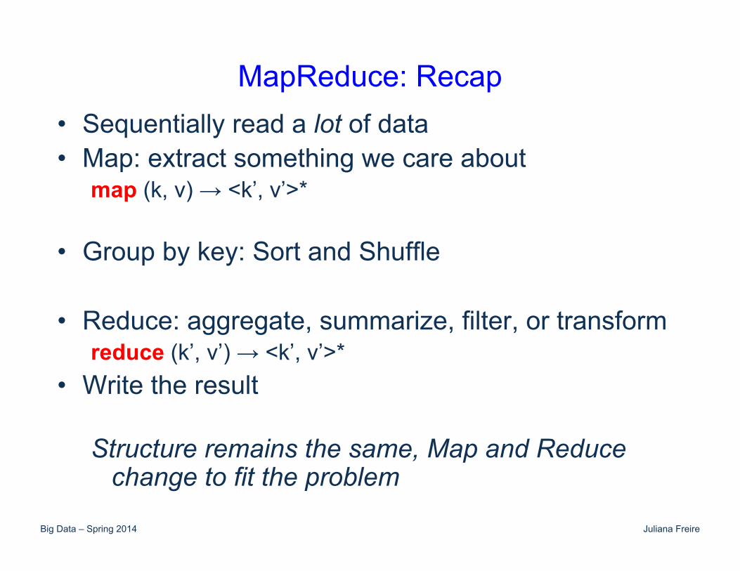
MapReduce: Recap • Sequentially read a lot of data • Map: extract something we care about
map (k, v) → <k’, v’>*
• Group by key: Sort and Shuffle
• Reduce: aggregate, summarize, filter, or transform reduce (k’, v’) → <k’, v’>*
• Write the result Structure remains the same, Map and Reduce
change to fit the problem
Big Data – Spring 2014 Juliana Freire
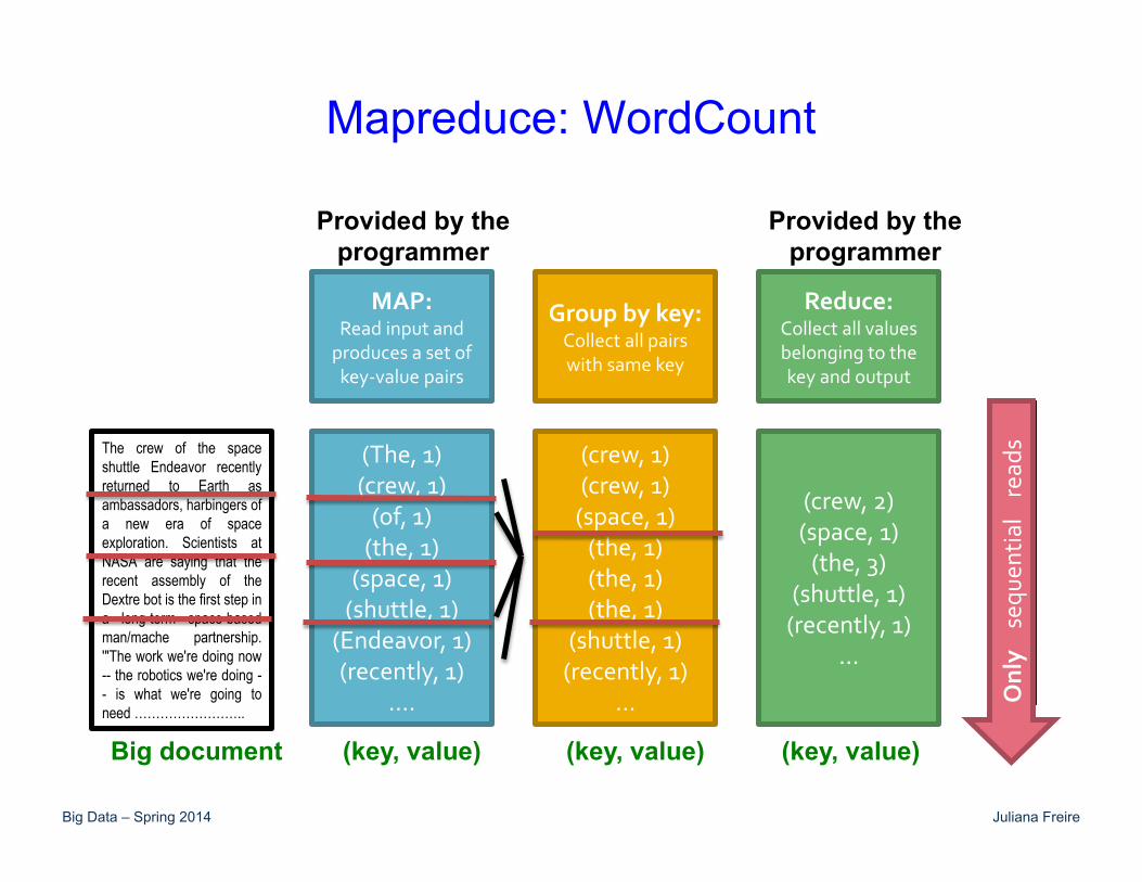
Mapreduce: WordCount
The crew of the space shuttle Endeavor recently returned to Earth as ambassadors, harbingers of a new era of space exploration. Scientists at NASA are saying that the recent assembly of the Dextre bot is the first step in a long-term space-based man/mache partnership. '"The work we're doing now -- the robotics we're doing -- is what we're going to need ……………………..
Big document
(The, 1) (crew, 1)
(of, 1) (the, 1)
(space, 1) (shuttle, 1)
(Endeavor, 1) (recently, 1)
….
(crew, 1) (crew, 1)
(space, 1) (the, 1) (the, 1) (the, 1)
(shuttle, 1) (recently, 1)
…
(crew, 2) (space, 1)
(the, 3) (shuttle, 1)
(recently, 1) …
MAP: Read input and
produces a set of key-value pairs
Group by key: Collect all pairs with same key
Reduce: Collect all values belonging to the key and output
(key, value)
Provided by the programmer
Provided by the programmer
(key, value) (key, value)
Sequ
entia
lly re
ad th
e da
ta
Onl
y
sequ
entia
l r
eads
1/8/2013 Jure Leskovec, Stanford CS246: Mining Massive Datasets, http://cs246.stanford.edu 40

Big Data – Spring 2014 Juliana Freire
MapReduce: Recap • Combiners combines the values of all keys of a
single mapper – Much less data needs to be shuffled
• Partition function: controls how keys get partitioned – Default: hash(key) mod R – Sometimes it is useful to override the default, e.g.,
hash(hostname(URL)) mod R ensures URLs from a host end up in the same output file
Big Data – Spring 2014 Juliana Freire
MapReduce: Environment Takes care of: • Partitioning the input data • Scheduling the execution of the program on multiple
machines • Performing the group by key step • Handling machine failures • Managing inter-machine communication
Big Data – Spring 2014 Juliana Freire
MapReduce: Data Flow • Input and final output are stored on the distributed
file system (DFS) – Scheduler tries to schedule map tasks “close” to physical
storage location of input data You can specify a directory where your input files reside using MultipleInputs.addInputPath
• Intermediate results are stored on local FS of Map and Reduce workers
• Output is often input to another MapReduce task
Big Data – Spring 2014 Juliana Freire
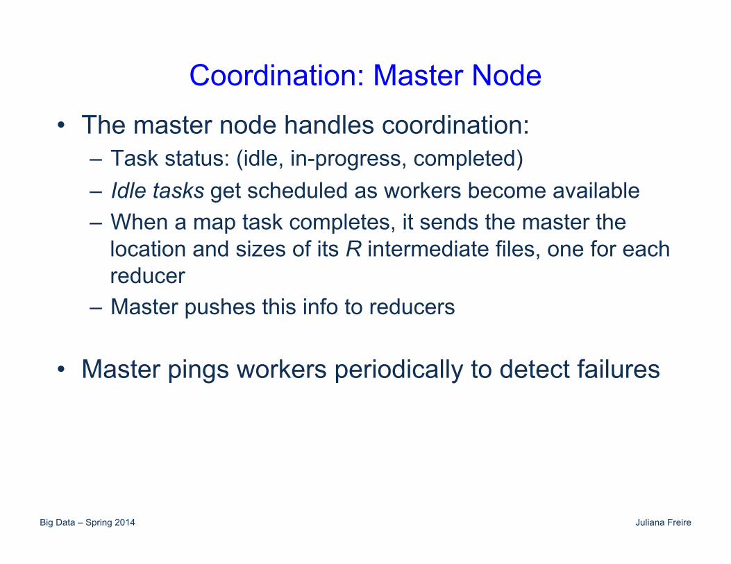
Coordination: Master Node • The master node handles coordination:
– Task status: (idle, in-progress, completed) – Idle tasks get scheduled as workers become available – When a map task completes, it sends the master the
location and sizes of its R intermediate files, one for each reducer
– Master pushes this info to reducers
• Master pings workers periodically to detect failures
Big Data – Spring 2014 Juliana Freire
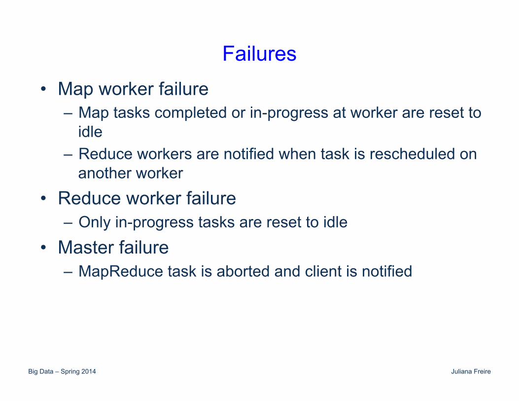
Failures • Map worker failure
– Map tasks completed or in-progress at worker are reset to idle
– Reduce workers are notified when task is rescheduled on another worker
• Reduce worker failure – Only in-progress tasks are reset to idle
• Master failure – MapReduce task is aborted and client is notified
Big Data – Spring 2014 Juliana Freire
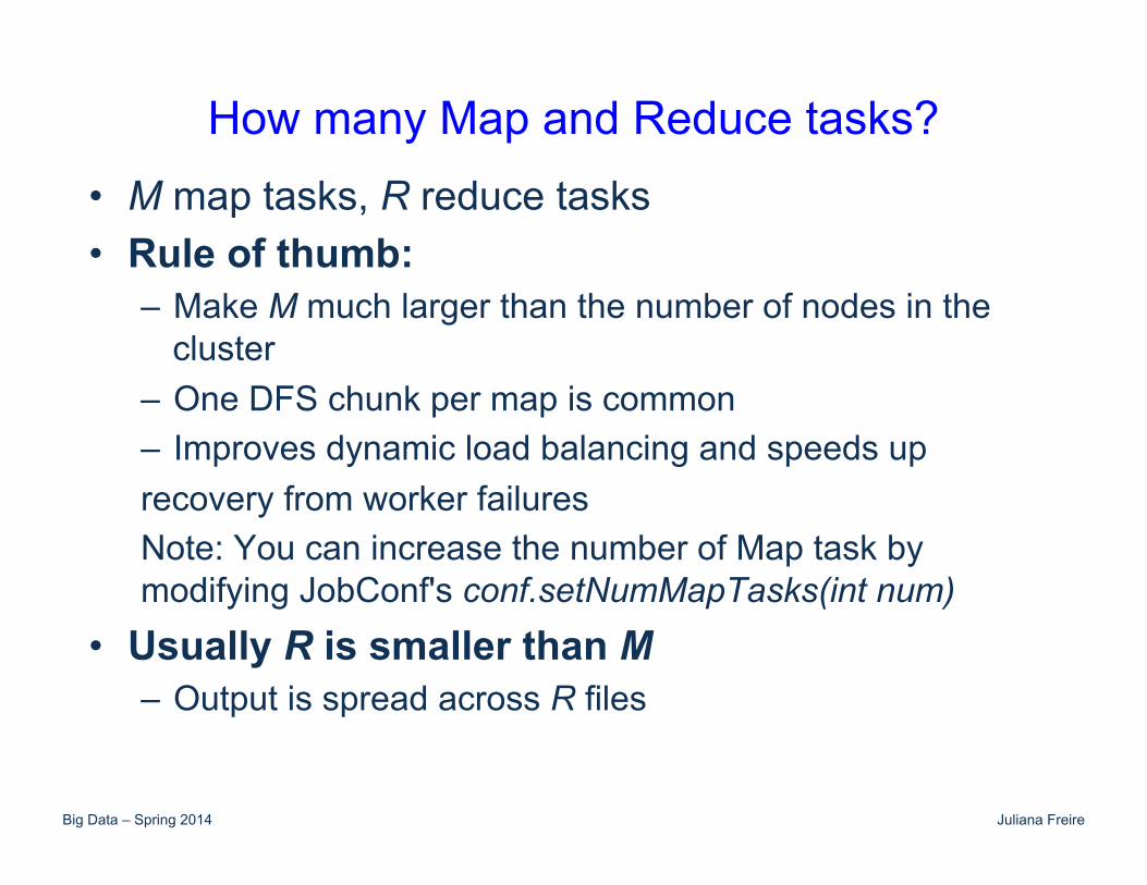
How many Map and Reduce tasks? • M map tasks, R reduce tasks • Rule of thumb:
– Make M much larger than the number of nodes in the cluster
– One DFS chunk per map is common – Improves dynamic load balancing and speeds up recovery from worker failures Note: You can increase the number of Map task by modifying JobConf's conf.setNumMapTasks(int num)
• Usually R is smaller than M – Output is spread across R files
Big Data – Spring 2014 Juliana Freire
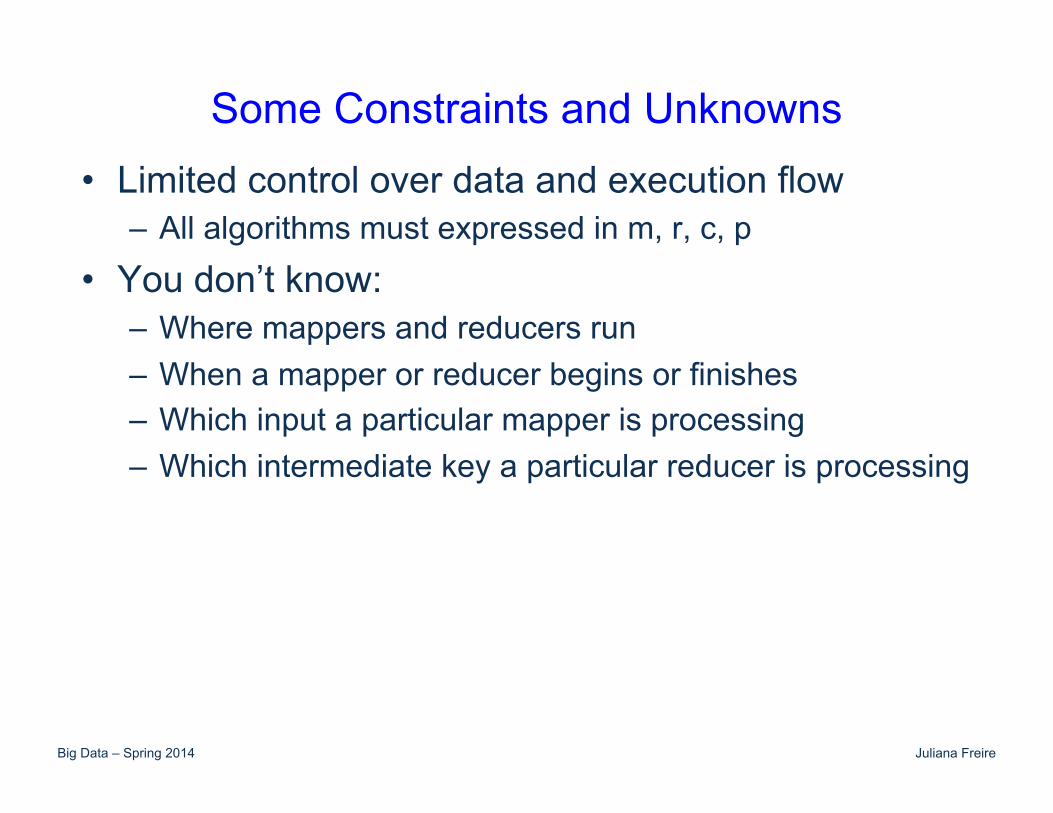
Some Constraints and Unknowns • Limited control over data and execution flow
– All algorithms must expressed in m, r, c, p
• You don’t know: – Where mappers and reducers run – When a mapper or reducer begins or finishes – Which input a particular mapper is processing – Which intermediate key a particular reducer is processing

Big Data – Spring 2014 Juliana Freire
Designing Algorithms for MapReduce • Need to adapt to a restricted model of computation • Goals
– Scalability: adding machines will make the algo run faster – Efficiency: resources will not be wasted
• The translation some algorithms into MapReduce isn’t always obvious
• But there are useful design patterns that can help • We will cover some and use examples to illustrate
how they can be applied
Big Data – Spring 2014 Juliana Freire
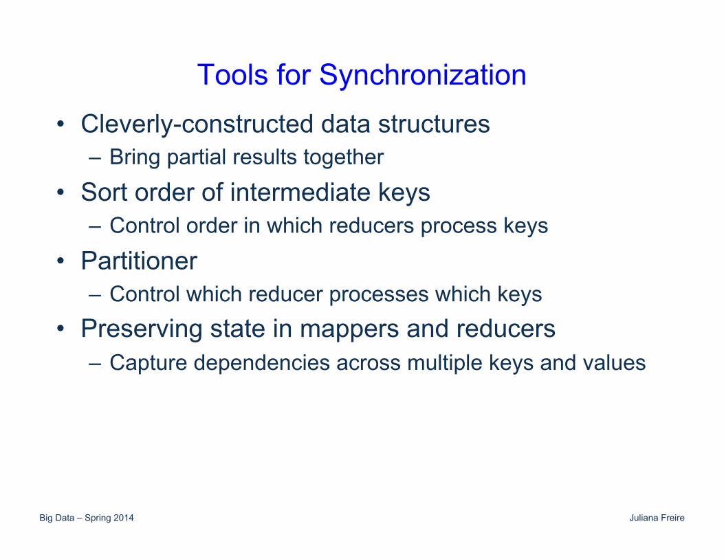
Tools for Synchronization • Cleverly-constructed data structures
– Bring partial results together
• Sort order of intermediate keys – Control order in which reducers process keys
• Partitioner – Control which reducer processes which keys
• Preserving state in mappers and reducers – Capture dependencies across multiple keys and values

Big Data – Spring 2014 Juliana Freire
Preserving State
Mapper object
configure
map
close
state one object per task
Reducer object
configure
reduce
close
state
one call per input key-value pair
one call per intermediate key
API initialization hook
API cleanup hook
Big Data – Spring 2014 Juliana Freire
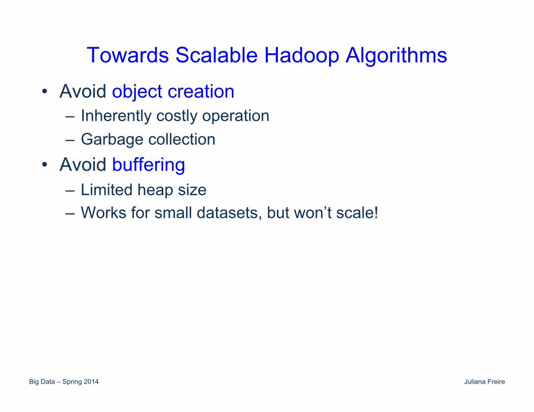
Towards Scalable Hadoop Algorithms • Avoid object creation
– Inherently costly operation – Garbage collection
• Avoid buffering – Limited heap size – Works for small datasets, but won’t scale!
Big Data – Spring 2014 Juliana Freire
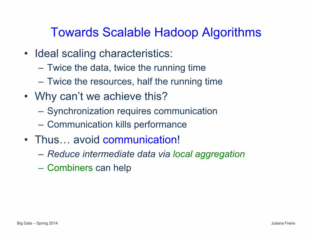
Towards Scalable Hadoop Algorithms • Ideal scaling characteristics:
– Twice the data, twice the running time – Twice the resources, half the running time
• Why can’t we achieve this? – Synchronization requires communication – Communication kills performance
• Thus… avoid communication! – Reduce intermediate data via local aggregation – Combiners can help
Big Data – Spring 2014 Juliana Freire
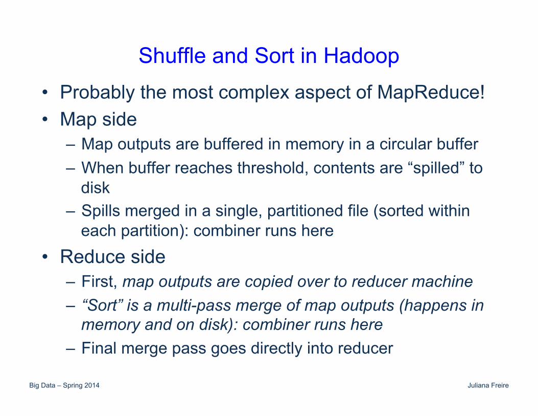
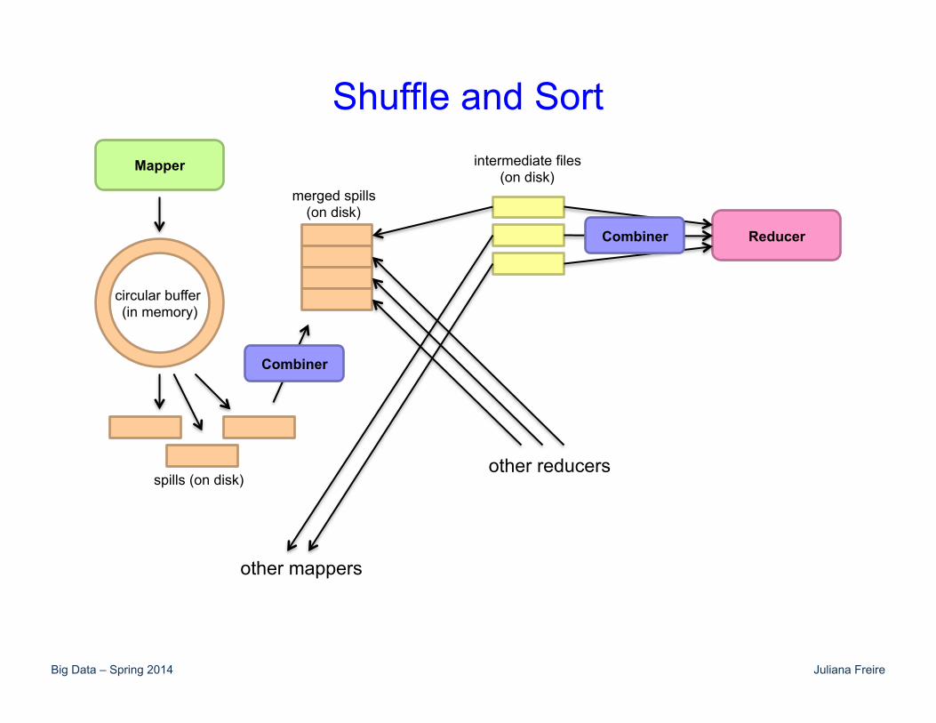
Shuffle and Sort in Hadoop • Probably the most complex aspect of MapReduce! • Map side
– Map outputs are buffered in memory in a circular buffer – When buffer reaches threshold, contents are “spilled” to
disk – Spills merged in a single, partitioned file (sorted within
each partition): combiner runs here • Reduce side
– First, map outputs are copied over to reducer machine – “Sort” is a multi-pass merge of map outputs (happens in
memory and on disk): combiner runs here – Final merge pass goes directly into reducer
Big Data – Spring 2014 Juliana Freire
Shuffle and Sort Mapper
Reducer
other mappers
other reducers
circular buffer (in memory)
spills (on disk)
merged spills (on disk)
intermediate files (on disk)
Combiner
Combiner

Big Data – Spring 2014 Juliana Freire
DESIGN PATTERNS
Big Data – Spring 2014 Juliana Freire
Strategy: Local Aggregation • Use combiners • Do aggregation inside mappers
Big Data – Spring 2014 Juliana Freire
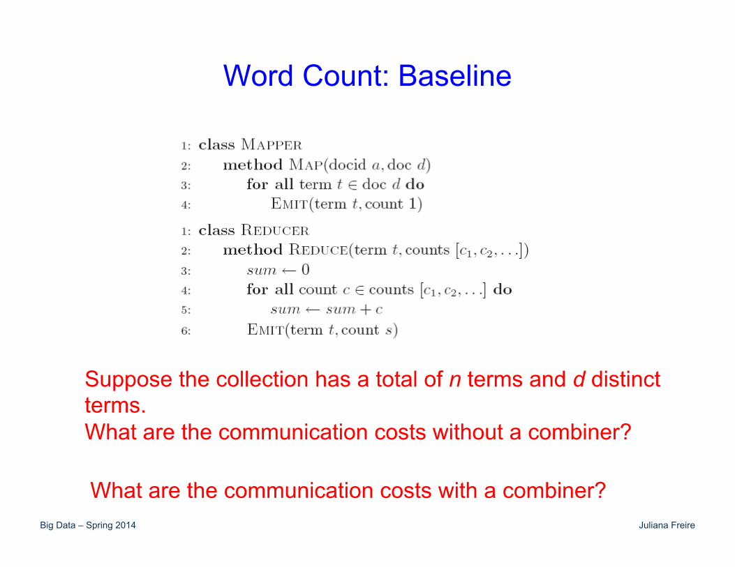
Word Count: Baseline
Suppose the collection has a total of n terms and d distinct terms. What are the communication costs without a combiner?
What are the communication costs with a combiner?
Big Data – Spring 2014 Juliana Freire
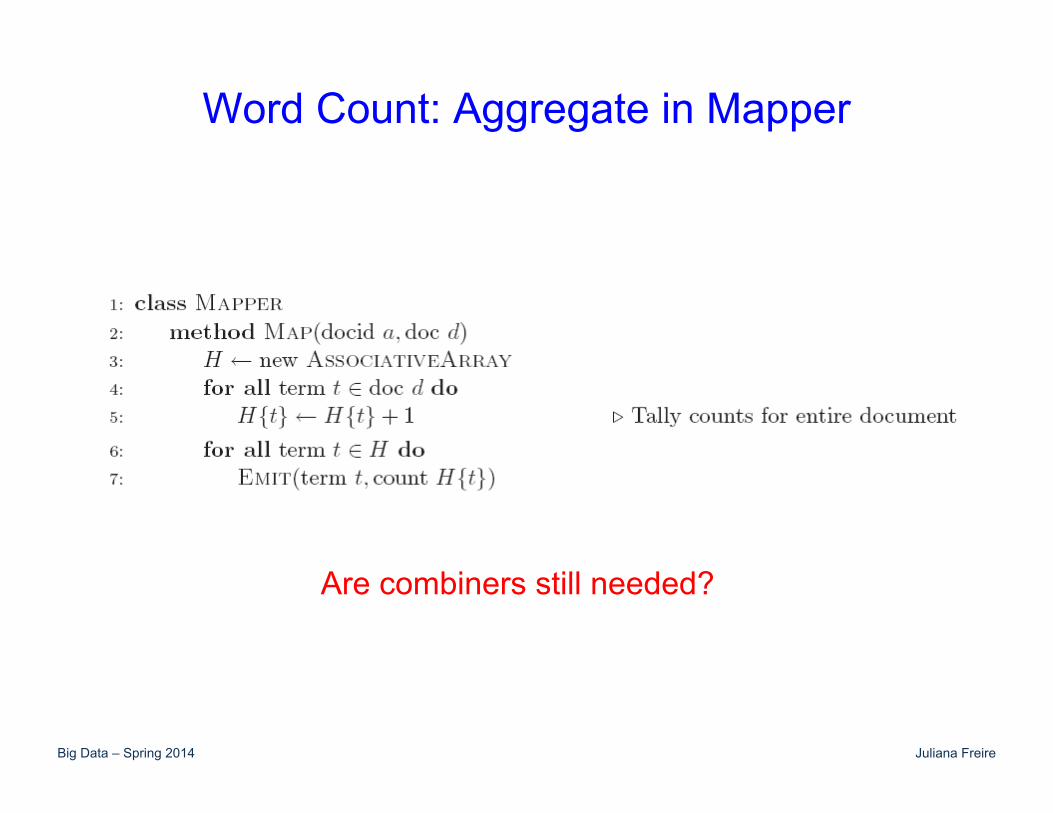
Word Count: Aggregate in Mapper
Are combiners still needed?

Big Data – Spring 2014 Juliana Freire
Word Count: Aggregate in Mapper (v 2)
Are combiners still needed?
Big Data – Spring 2014 Juliana Freire
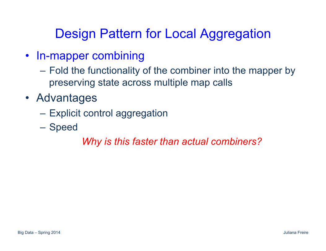
Design Pattern for Local Aggregation • In-mapper combining
– Fold the functionality of the combiner into the mapper by preserving state across multiple map calls
• Advantages – Explicit control aggregation – Speed
Why is this faster than actual combiners?
Big Data – Spring 2014 Juliana Freire
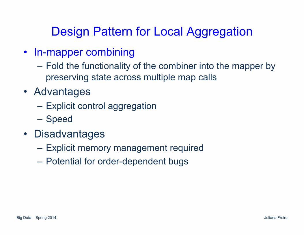
Design Pattern for Local Aggregation • In-mapper combining
– Fold the functionality of the combiner into the mapper by preserving state across multiple map calls
• Advantages – Explicit control aggregation – Speed
• Disadvantages – Explicit memory management required – Potential for order-dependent bugs
Big Data – Spring 2014 Juliana Freire
Limiting Memory Usage • To limit memory usage when using the in-mapper
combining technique, block input key-value pairs and flush in-memory data structures periodically – E.g., counter variable that keeps track of the number of input
key-value pairs that have been processed
• Memory usage threshold needs to be determined empirically: with too large a value, the mapper may run out of memory, but with too small a value, opportunities for local aggregation may be lost
• Note: Hadoop physical memory is split between multiple tasks that may be running on a node concurrently – difficult to coordinate resource consumption
Big Data – Spring 2014 Juliana Freire
Combiner Design • Combiners and reducers share same method
signature – Sometimes, reducers can serve as combiners
When is this the case?
Big Data – Spring 2014 Juliana Freire
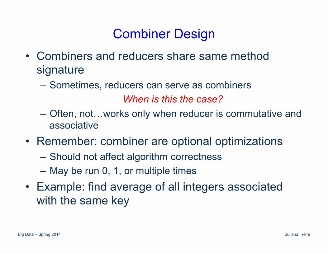
Combiner Design • Combiners and reducers share same method
signature – Sometimes, reducers can serve as combiners
When is this the case? – Often, not…works only when reducer is commutative and
associative • Remember: combiner are optional optimizations
– Should not affect algorithm correctness – May be run 0, 1, or multiple times
• Example: find average of all integers associated with the same key
Big Data – Spring 2014 Juliana Freire
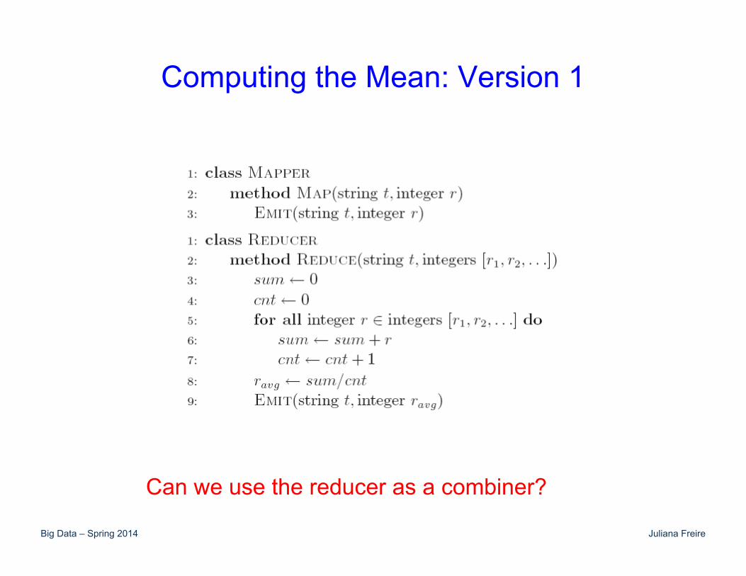
Computing the Mean: Version 1
Can we use the reducer as a combiner?
Big Data – Spring 2014 Juliana Freire
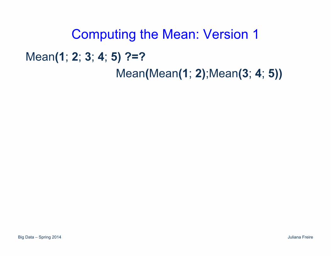
Computing the Mean: Version 1 Mean(1; 2; 3; 4; 5) ?=? Mean(Mean(1; 2);Mean(3; 4; 5))
Big Data – Spring 2014 Juliana Freire
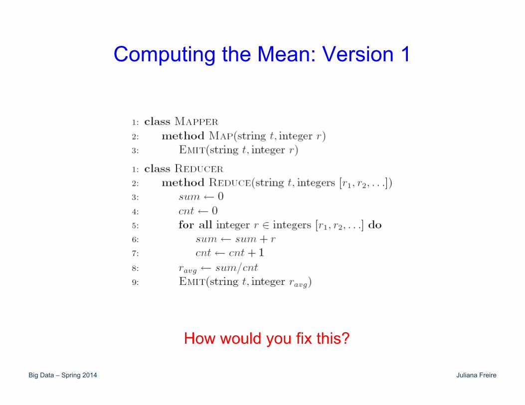
Computing the Mean: Version 1
How would you fix this?
Big Data – Spring 2014 Juliana Freire
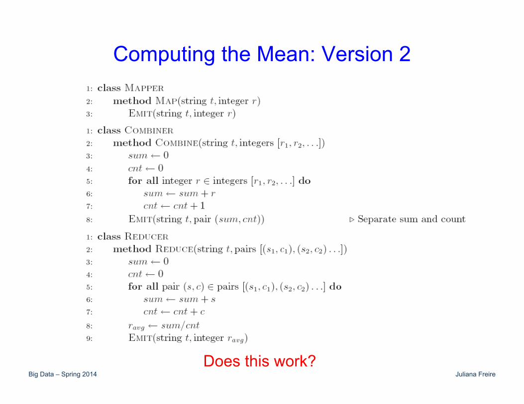
Computing the Mean: Version 2
Does this work?
Big Data – Spring 2014 Juliana Freire
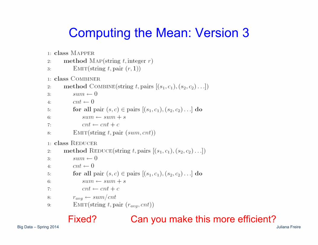
Computing the Mean: Version 3
Fixed? Can you make this more efficient?
Big Data – Spring 2014 Juliana Freire
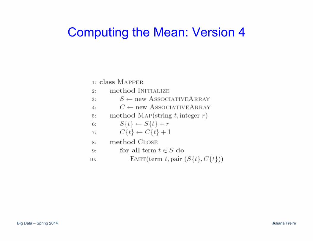
Computing the Mean: Version 4
Big Data – Spring 2014 Juliana Freire
Algorithm Design: Running Example • Term co-occurrence matrix for a text collection
– M = N x N matrix (N = vocabulary size) – Mij: number of times i and j co-occur in some context
(for concreteness, let’s say context = sentence) • Why?
– Distributional profiles as a way of measuring semantic distance
– Semantic distance useful for many language processing tasks
Big Data – Spring 2014 Juliana Freire
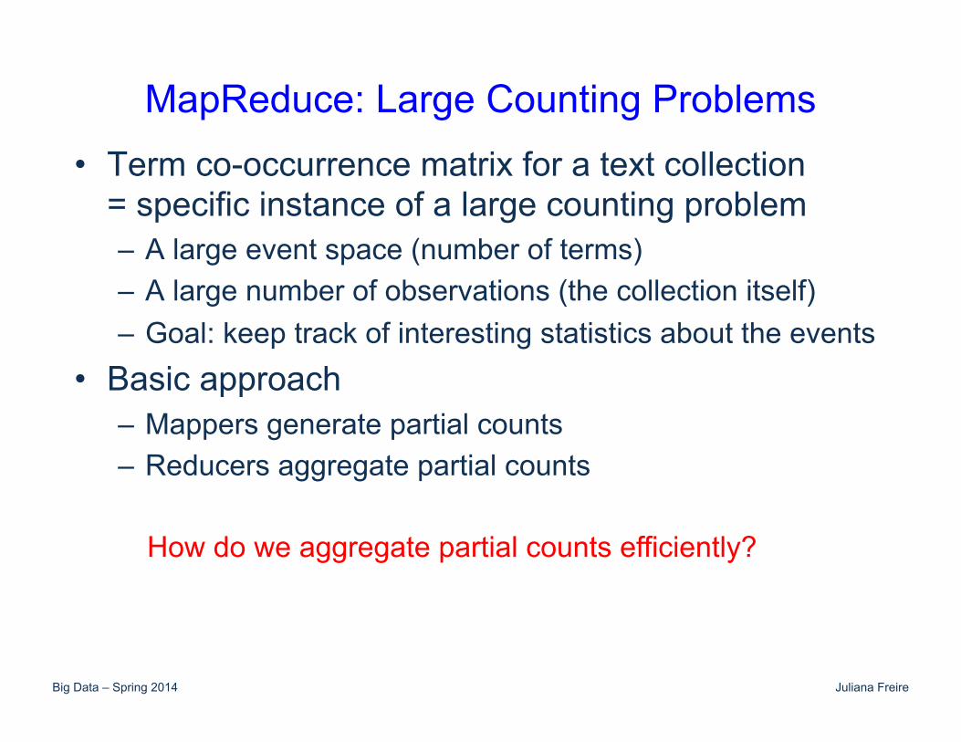
MapReduce: Large Counting Problems • Term co-occurrence matrix for a text collection
= specific instance of a large counting problem – A large event space (number of terms) – A large number of observations (the collection itself) – Goal: keep track of interesting statistics about the events
• Basic approach – Mappers generate partial counts – Reducers aggregate partial counts
How do we aggregate partial counts efficiently?
Big Data – Spring 2014 Juliana Freire
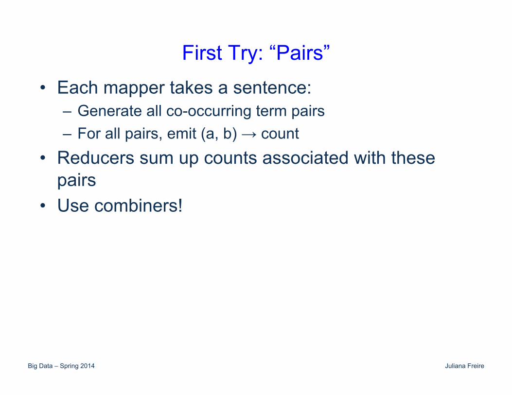
First Try: “Pairs” • Each mapper takes a sentence:
– Generate all co-occurring term pairs – For all pairs, emit (a, b) → count
• Reducers sum up counts associated with these pairs
• Use combiners!
Big Data – Spring 2014 Juliana Freire
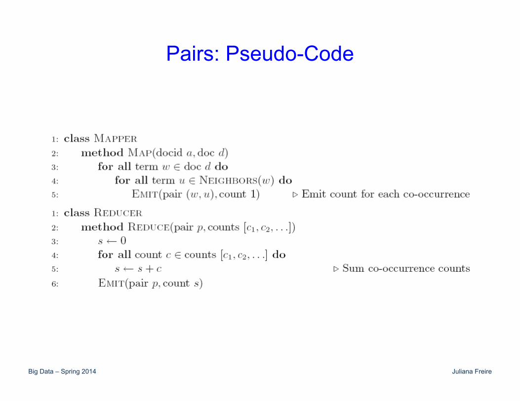
Pairs: Pseudo-Code
Big Data – Spring 2014 Juliana Freire
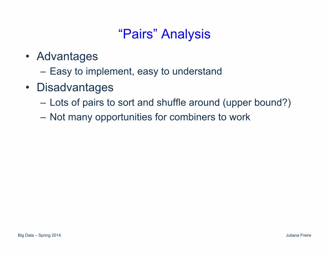
“Pairs” Analysis • Advantages
– Easy to implement, easy to understand
• Disadvantages – Lots of pairs to sort and shuffle around (upper bound?) – Not many opportunities for combiners to work
Big Data – Spring 2014 Juliana Freire
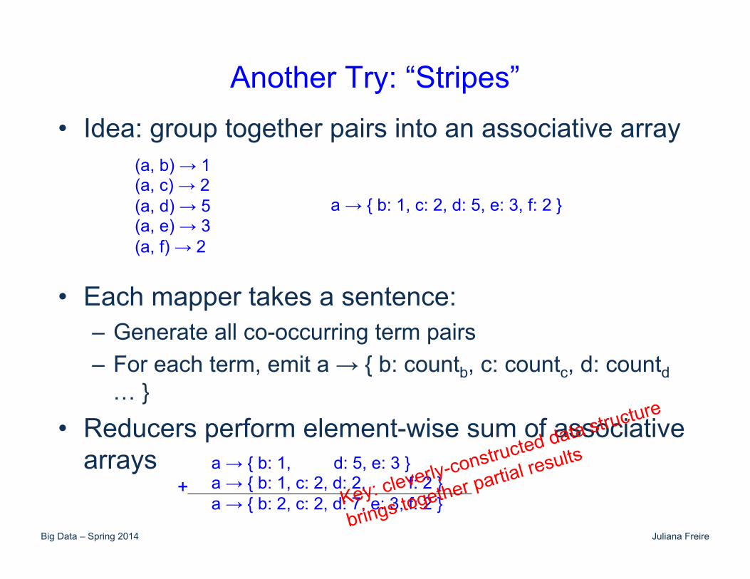
Another Try: “Stripes” • Idea: group together pairs into an associative array
• Each mapper takes a sentence: – Generate all co-occurring term pairs – For each term, emit a → { b: countb, c: countc, d: countd … }
• Reducers perform element-wise sum of associative arrays
(a, b) → 1 (a, c) → 2 (a, d) → 5 (a, e) → 3 (a, f) → 2
a → { b: 1, c: 2, d: 5, e: 3, f: 2 }
a → { b: 1, d: 5, e: 3 } a → { b: 1, c: 2, d: 2, f: 2 } a → { b: 2, c: 2, d: 7, e: 3, f: 2 }
+ Key: cleverly-constructed data structure
brings together partial results
Big Data – Spring 2014 Juliana Freire
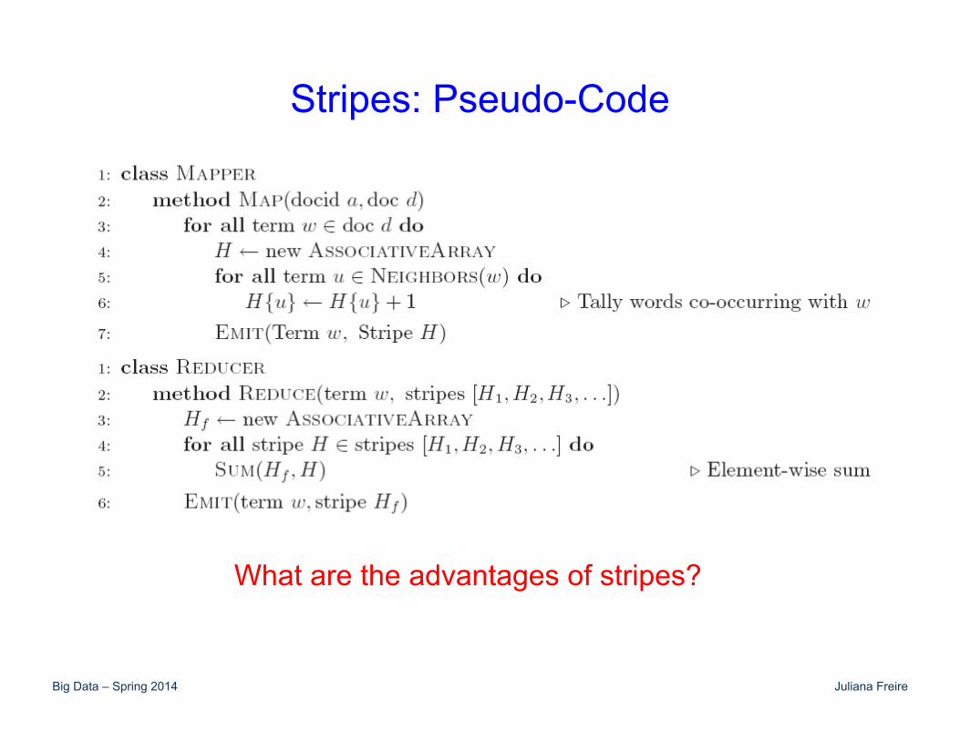
Stripes: Pseudo-Code
What are the advantages of stripes?
Big Data – Spring 2014 Juliana Freire
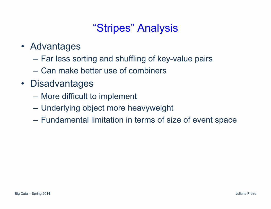
“Stripes” Analysis • Advantages
– Far less sorting and shuffling of key-value pairs – Can make better use of combiners
• Disadvantages – More difficult to implement – Underlying object more heavyweight – Fundamental limitation in terms of size of event space
Big Data – Spring 2014 Juliana Freire
What about combiners? • Both algorithms can benefit from the use of combiners,
since the respective operations in their reducers (addition and element-wise sum of associative arrays) are both commutative and associative.
• Are combiners equally effective in both pairs and stripes?

Big Data – Spring 2014 Juliana Freire
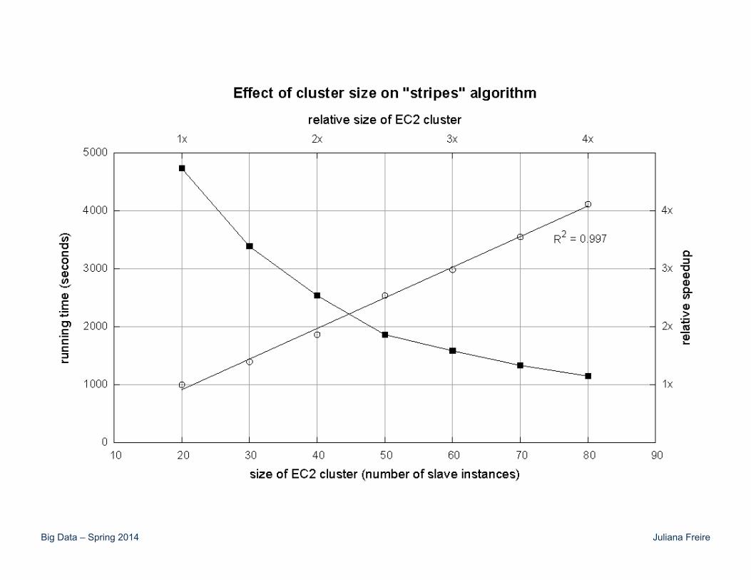
Cluster size: 38 cores Data Source: Associated Press Worldstream (APW) of the English Gigaword Corpus (v3), which contains 2.27 million documents (1.8 GB compressed, 5.7 GB uncompressed)
Big Data – Spring 2014 Juliana Freire

Big Data – Spring 2014 Juliana Freire
Relative Frequencies • How do we estimate relative frequencies from
counts?
• Why do we want to do this? • How do we do this with MapReduce?
∑==
')',(count),(count
)(count),(count)|(
BBABA
ABAABf
Big Data – Spring 2014 Juliana Freire
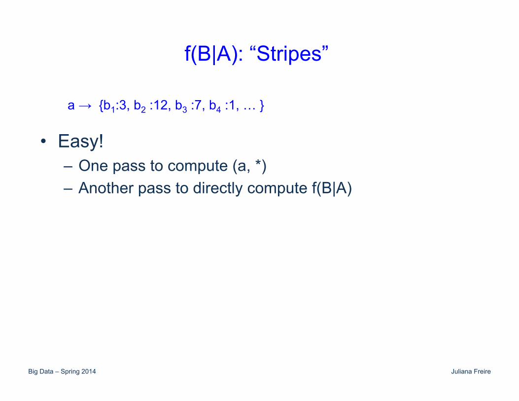
f(B|A): “Stripes”
• Easy! – One pass to compute (a, *) – Another pass to directly compute f(B|A)
a → {b1:3, b2 :12, b3 :7, b4 :1, … }

Big Data – Spring 2014 Juliana Freire
f(B|A): “Pairs”
• For this to work: – Must emit extra (a, *) for every bn in mapper – Must make sure all a’s get sent to same reducer (use
partitioner) – Must make sure (a, *) comes first (define sort order) – Must hold state in reducer across different key-value pairs
(a, b1) → 3 (a, b2) → 12 (a, b3) → 7 (a, b4) → 1 …
(a, *) → 32
(a, b1) → 3 / 32 (a, b2) → 12 / 32 (a, b3) → 7 / 32 (a, b4) → 1 / 32 …
Reducer holds this value in memory
Big Data – Spring 2014 Juliana Freire
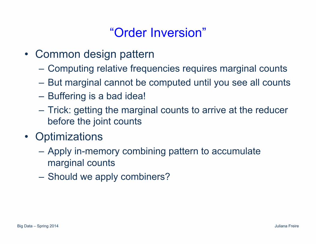
“Order Inversion” • Common design pattern
– Computing relative frequencies requires marginal counts – But marginal cannot be computed until you see all counts – Buffering is a bad idea! – Trick: getting the marginal counts to arrive at the reducer
before the joint counts • Optimizations
– Apply in-memory combining pattern to accumulate marginal counts
– Should we apply combiners?
Big Data – Spring 2014 Juliana Freire
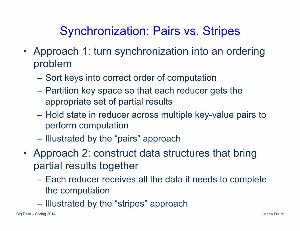
Synchronization: Pairs vs. Stripes • Approach 1: turn synchronization into an ordering
problem – Sort keys into correct order of computation – Partition key space so that each reducer gets the
appropriate set of partial results – Hold state in reducer across multiple key-value pairs to
perform computation – Illustrated by the “pairs” approach
• Approach 2: construct data structures that bring partial results together – Each reducer receives all the data it needs to complete
the computation – Illustrated by the “stripes” approach

Big Data – Spring 2014 Juliana Freire
Secondary Sorting • MapReduce sorts input to reducers by key
– Values may be arbitrarily ordered
• What if want to sort value also? – E.g., k → (v1, r), (v3, r), (v4, r), (v8, r)…
Big Data – Spring 2014 Juliana Freire
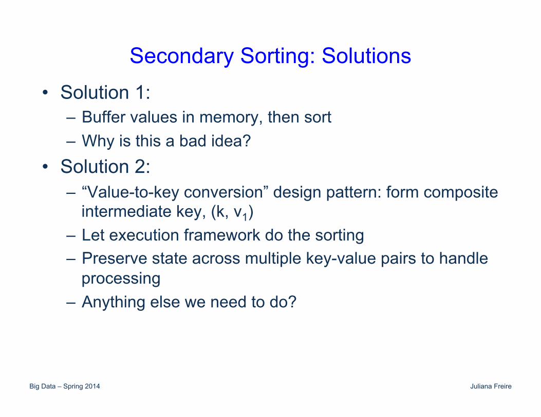
Secondary Sorting: Solutions • Solution 1:
– Buffer values in memory, then sort – Why is this a bad idea?
• Solution 2: – “Value-to-key conversion” design pattern: form composite
intermediate key, (k, v1) – Let execution framework do the sorting – Preserve state across multiple key-value pairs to handle
processing – Anything else we need to do?
Big Data – Spring 2014 Juliana Freire
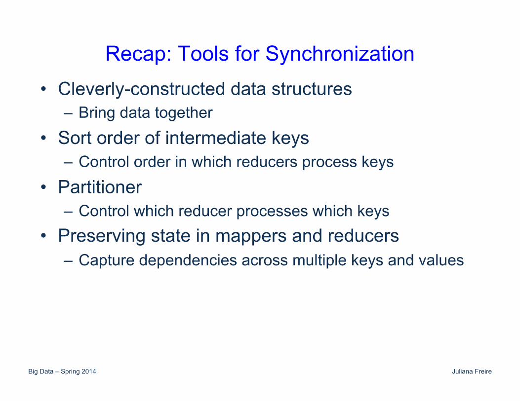
Recap: Tools for Synchronization • Cleverly-constructed data structures
– Bring data together
• Sort order of intermediate keys – Control order in which reducers process keys
• Partitioner – Control which reducer processes which keys
• Preserving state in mappers and reducers – Capture dependencies across multiple keys and values
Big Data – Spring 2014 Juliana Freire
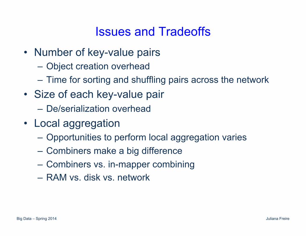
Issues and Tradeoffs • Number of key-value pairs
– Object creation overhead – Time for sorting and shuffling pairs across the network
• Size of each key-value pair – De/serialization overhead
• Local aggregation – Opportunities to perform local aggregation varies – Combiners make a big difference – Combiners vs. in-mapper combining – RAM vs. disk vs. network
Big Data – Spring 2014 Juliana Freire
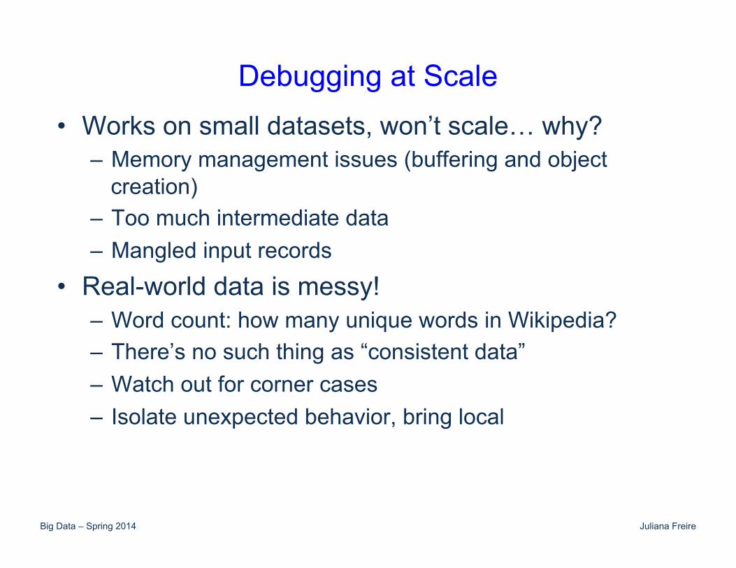
Debugging at Scale • Works on small datasets, won’t scale… why?
– Memory management issues (buffering and object creation)
– Too much intermediate data – Mangled input records
• Real-world data is messy! – Word count: how many unique words in Wikipedia? – There’s no such thing as “consistent data” – Watch out for corner cases – Isolate unexpected behavior, bring local

Big Data – Spring 2014 Juliana Freire
REASONING ABOUT COST

Big Data – Spring 2014 Juliana Freire
Cost Measures for Algorithms 1. Communication cost = total I/O of all processes. 2. Elapsed communication cost = max of I/O along
any path. 3. (Elapsed ) computation costs analogous, but
count only running time of processes.
Big Data – Spring 2014 Juliana Freire
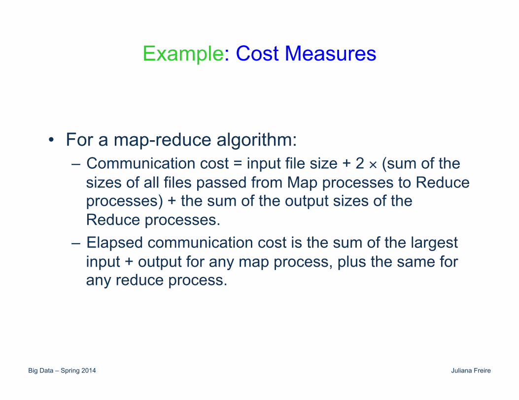
Example: Cost Measures
• For a map-reduce algorithm: – Communication cost = input file size + 2 × (sum of the
sizes of all files passed from Map processes to Reduce processes) + the sum of the output sizes of the Reduce processes.
– Elapsed communication cost is the sum of the largest input + output for any map process, plus the same for any reduce process.

Big Data – Spring 2014 Juliana Freire
What Cost Measures Mean
• Either the I/O (communication) or processing (computation) cost dominates. – Ignore one or the other.
• Total costs tell what you pay in rent from your friendly neighborhood cloud.
• Elapsed costs are wall-clock time using parallelism.

Big Data – Spring 2014 Juliana Freire
JOINS IN MAPREDUCE
Big Data – Spring 2014 Juliana Freire
Join By Map-Reduce • Our first example of an algorithm in this framework
is a map-reduce example.
• Compute the natural join R(A,B) ⋈ S(B,C). • R and S each are stored in files. • Tuples are pairs (a,b) or (b,c).

Big Data – Spring 2014 Juliana Freire
Map-Reduce Join – (2) • Use a hash function h from B-values to 1..k. • A Map process turns input tuple R(a,b) into key-
value pair (b,(a,R)) and each input tuple S(b,c) into (b,(c,S)).
Big Data – Spring 2014 Juliana Freire
Map-Reduce Join – (3) • Map processes send each key-value pair with key b
to Reduce process h(b). – Hadoop does this automatically; just tell it what k is.
• Each Reduce process matches all the pairs (b,(a,R)) with all (b,(c,S)) and outputs (a,b,c).

Big Data – Spring 2014 Juliana Freire
Cost of Map-Reduce Join
• Total communication cost = O(|R|+|S|+|R ⋈ S|). • Elapsed communication cost = O(s ).
– We’re going to pick k and the number of Map processes so I/O limit s is respected.
– We put a limit s on the amount of input or output that any one process can have. s could be:
• What fits in main memory • What fits on local disk
• With proper indexes, computation cost is linear in the input + output size. – So computation costs are like communication costs.
Big Data – Spring 2014 Juliana Freire
Three-Way Join • We shall consider a simple join of three relations,
the natural join R(A,B) ⋈ S(B,C) ⋈ T(C,D). • One way: cascade of two 2-way joins, each
implemented by map-reduce. • Fine, unless the 2-way joins produce large
intermediate relations.
Big Data – Spring 2014 Juliana Freire 66
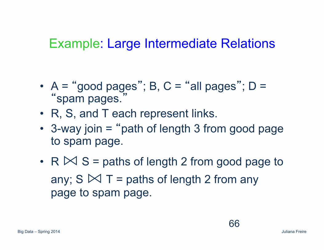
Example: Large Intermediate Relations
• A = “good pages”; B, C = “all pages”; D = “spam pages.”
• R, S, and T each represent links. • 3-way join = “path of length 3 from good page
to spam page.
• R ⋈ S = paths of length 2 from good page to any; S ⋈ T = paths of length 2 from any page to spam page.
Big Data – Spring 2014 Juliana Freire 67
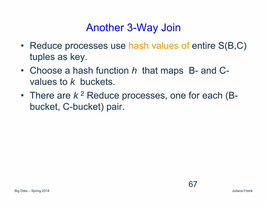
Another 3-Way Join • Reduce processes use hash values of entire S(B,C)
tuples as key. • Choose a hash function h that maps B- and C-
values to k buckets. • There are k 2 Reduce processes, one for each (B-
bucket, C-bucket) pair.

Big Data – Spring 2014 Juliana Freire 68
Mapping for 3-Way Join
• We map each tuple S(b,c) to ((h(b), h(c)), (S, b, c)). • We map each R(a,b) tuple to
((h(b), y), (R, a, b)) for all y = 1, 2,…,k. • We map each T(c,d) tuple to
((x, h(c)), (T, c, d)) for all x = 1, 2,…,k.
Keys Values
Big Data – Spring 2014 Juliana Freire 69
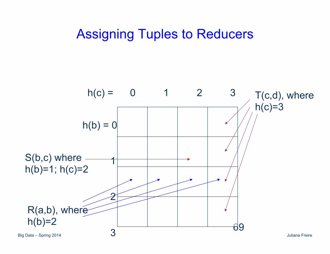
Assigning Tuples to Reducers
h(b) = 0 1 2 3
h(c) = 0 1 2 3
S(b,c) where h(b)=1; h(c)=2
R(a,b), where h(b)=2
T(c,d), where h(c)=3
Big Data – Spring 2014 Juliana Freire 70
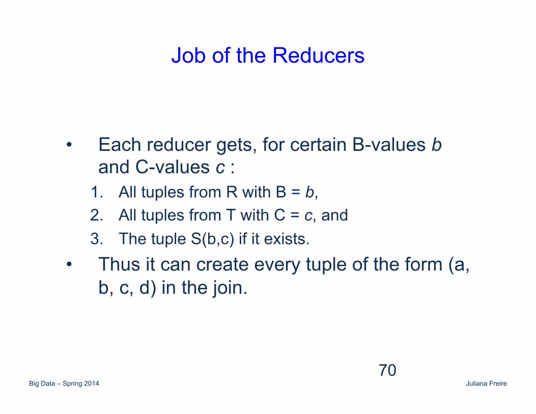
Job of the Reducers
• Each reducer gets, for certain B-values b and C-values c :
1. All tuples from R with B = b, 2. All tuples from T with C = c, and 3. The tuple S(b,c) if it exists.
• Thus it can create every tuple of the form (a, b, c, d) in the join.

Big Data – Spring 2014 Juliana Freire
RUNNING MAPREDUCE JOBS
Big Data – Spring 2014 Juliana Freire
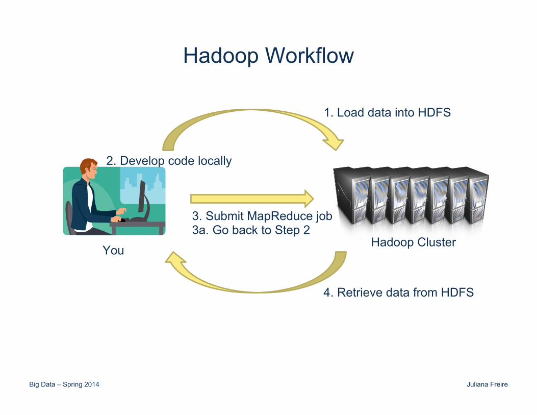
Hadoop Workflow
Hadoop Cluster You
1. Load data into HDFS
2. Develop code locally
3. Submit MapReduce job 3a. Go back to Step 2
4. Retrieve data from HDFS
Big Data – Spring 2014 Juliana Freire
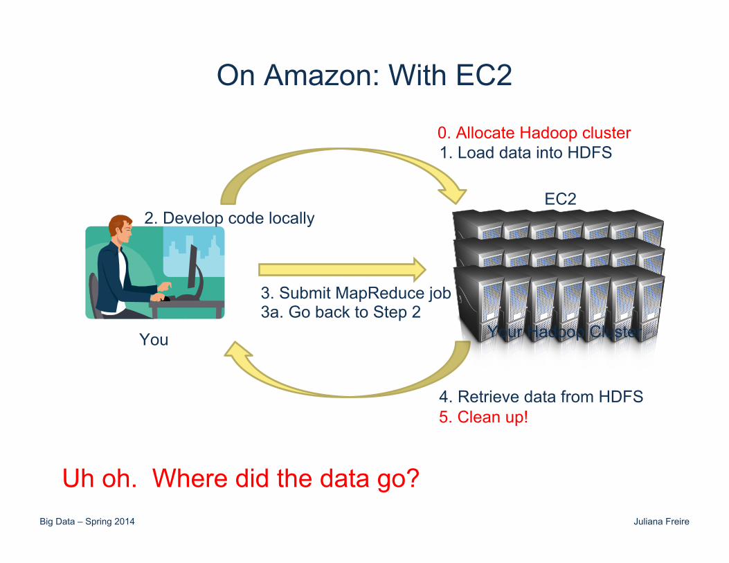
On Amazon: With EC2
You
1. Load data into HDFS
2. Develop code locally
3. Submit MapReduce job 3a. Go back to Step 2
4. Retrieve data from HDFS
0. Allocate Hadoop cluster
EC2
Your Hadoop Cluster
5. Clean up!
Uh oh. Where did the data go?
Big Data – Spring 2014 Juliana Freire
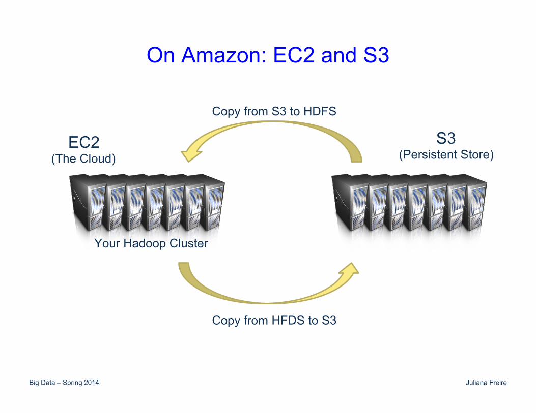
On Amazon: EC2 and S3
Your Hadoop Cluster
S3 (Persistent Store)
EC2 (The Cloud)
Copy from S3 to HDFS
Copy from HFDS to S3
Big Data – Spring 2014 Juliana Freire
Debugging Hadoop • First, take a deep breath • Start small, start locally • Strategies
– Learn to use the webapp – Where does println go? – Don’t use println, use logging – Throw RuntimeExceptions
Big Data – Spring 2014 Juliana Freire
Discussion About Assignment 2 • Constraints are your friends, in their absence the
semantics can be confusing • In your assignment, the tables did not have keys or
foreign keys – Join on station name was problematic
• Real data is messy, noisy • When you get data from different sources, you need
to be careful about combining them – Set of stations in one table was different from the other

Big Data – Spring 2014 Juliana Freire
References
• Data Intensive Text Processing with MapReduce, Lin and Dyer (Chapter 3)
• Mining of Massive Data Sets, Rajaraman et al. (Chapter 2)