Mappings to Polygonal Domains - jimrolf.com · Mappings to Polygonal Domains Jane McDougall and...
53
CHAPTER 5 Mappings to Polygonal Domains Jane McDougall and Lisbeth Schaubroeck (text), Jim Rolf (applets) 5.1. Introduction A rich source of problems in analysis is determining when, and how, one can create a one-to-one function of a particular type from one region onto another. In this chapter, we consider the problem of mapping the unit disk D onto a polygonal domain by two different classes of functions. First for analytic functions we give an overview and examples of the well known Schwarz-Christoffel transformation. We then diverge from analytic function theory and consider the Poisson integral formula to find harmonic functions that will serve as mapping functions onto polygonal domains. Proving that these harmonic functions are univalent requires us to explore some less known theory of harmonic functions and some relatively new techniques. Because of the Riemann Mapping Theorem, we can simplify our mapping problem for either class of function to asking when we can map the unit disk D = {z : |z | < 1} univalently onto a target region. This is because if we want to map one domain (other than the entire set of complex numbers) onto another, we can first map it to D by an analytic function, and subsequently apply an analytic or harmonic mapping from D to the other domain (recall that the composition of a harmonic function with an analytic function is harmonic). We begin in Section 1.2 with the Schwarz-Christoffel formula to find univalent analytic maps onto polygonal domains, and so set the stage for the corresponding problem for harmonic functions with the Poisson integral formula in Section 1.3. Per- haps because of their importance in applications, many first books on complex analysis introduce Schwarz-Christoffel mappings through examples, without emphasis on sub- tleties of the deeper theory. Our approach here will be the same, and the examples we include are chosen to bring together ideas found elsewhere in this book, such as the shearing technique from Chapter 4 and the construction of minimal surfaces from Chapter 5. We also include an example of a Schwarz-Christoffel map onto a regular star, a polygonal domain that is highly symmetric but also non-convex. The problem of using the Poisson integral formula to construct a univalent harmonic function onto a non- convex domain is not at all well understood. In Section 1.3, after developing the theory 322
Transcript of Mappings to Polygonal Domains - jimrolf.com · Mappings to Polygonal Domains Jane McDougall and...
CHAPTER 5
Mappings to Polygonal Domains
Jane McDougall and Lisbeth Schaubroeck (text), Jim Rolf (applets)
5.1. Introduction
A rich source of problems in analysis is determining when, and how, one can createa one-to-one function of a particular type from one region onto another. In this chapter,we consider the problem of mapping the unit disk D onto a polygonal domain by twodifferent classes of functions. First for analytic functions we give an overview andexamples of the well known Schwarz-Christoffel transformation. We then diverge fromanalytic function theory and consider the Poisson integral formula to find harmonicfunctions that will serve as mapping functions onto polygonal domains. Proving thatthese harmonic functions are univalent requires us to explore some less known theoryof harmonic functions and some relatively new techniques.
Because of the Riemann Mapping Theorem, we can simplify our mapping problemfor either class of function to asking when we can map the unit disk D = z : |z| < 1univalently onto a target region. This is because if we want to map one domain (otherthan the entire set of complex numbers) onto another, we can first map it to D by ananalytic function, and subsequently apply an analytic or harmonic mapping from D tothe other domain (recall that the composition of a harmonic function with an analyticfunction is harmonic).
We begin in Section 1.2 with the Schwarz-Christoffel formula to find univalentanalytic maps onto polygonal domains, and so set the stage for the correspondingproblem for harmonic functions with the Poisson integral formula in Section 1.3. Per-haps because of their importance in applications, many first books on complex analysisintroduce Schwarz-Christoffel mappings through examples, without emphasis on sub-tleties of the deeper theory. Our approach here will be the same, and the exampleswe include are chosen to bring together ideas found elsewhere in this book, such asthe shearing technique from Chapter 4 and the construction of minimal surfaces fromChapter 5.
We also include an example of a Schwarz-Christoffel map onto a regular star, apolygonal domain that is highly symmetric but also non-convex. The problem of usingthe Poisson integral formula to construct a univalent harmonic function onto a non-convex domain is not at all well understood. In Section 1.3, after developing the theory
322
for convex domains, we explore the example of finding harmonic maps onto regular stardomains in detail, and lead the student to further investigation.
Terminology and technology: We use the term “univalent” for one-to-one, and takedomain to mean open connected set in the complex plane. The applets used in thischapter are:
(1) ComplexTool - used to plot the image of domains in C under complex-valuedfunctions.
(2) PolyTool - used to visualize the harmonic function that is the extension ofa particular kind of boundary correspondence. The user of this applet candynamically change the boundary correspondence and watch the harmonicfunction change.
(3) StarTool - used to examine the functions that map the unit disk D onto ann-pointed star. The user can modify the shape of the star (by changing n andr) and the boundary correspondence (by changing p).
5.2. Schwarz-Christoffel Maps
In this section we consider conformal maps from the unit disk and the upper half-plane onto various simply connected polygonal domains. By the Riemann MappingTheorem, we can map the unit disk conformally onto any simply connected domainthat is a proper subset of the complex numbers, with a mapping function that isessentially unique.
While the Riemann Mapping Theorem tells us that we can find a univalent analyticfunction to map D onto our domain, finding an actual Riemann mapping function is noeasy task. Even for a simple domain such as a square, the mapping function from thedisk cannot be expressed in terms of elementary functions. One situation however inwhich this problem is relatively simple is in mapping a region bounded by a circle or linein the complex plane to another such region, using fractional linear transformations.For this problem, we only need to pick three points on the bounding line or circle in thedomain, and map them (in order) to three arbitrarily chosen points on the boundaryof the target region (see for example [10], [15], [19], or [20]). This selection of threepairs of points determines the fractional linear transformation completely, and worksfor example, in finding a conformal map from D onto any planar region bounded by aline or circle.
Exercise 5.1. Show that the fractional linear transformation z′ = φ (z) = i1+z1−z
maps the unit disk to the upper half-plane by finding the images of three boundarypoints. Then show that its inverse function φ−1(z′) = z = z′−i
z′+imaps the upper half-
plane to the unit disk. Try it out!
How can a mapping function be found in the case when the target region is morecomplicated? This question is relevant to solving the heat equation or the study offluid flows, as discussed in Chapter 3.
323

The Schwarz-Christoffel transformation frequently enables us to find a functionmapping onto a polygonal domain. In most texts the formula is presented as a mappingfrom the upper half-plane H onto the target polygon. We now develop this formula -for a more thorough treatment we refer the reader to [13], [3] and [16]. Suppose ourtarget polygon has interior angles αkπ and exterior angles βkπ, where αk +βk = 1 andαk > 0. The exterior angle measures the angle through which a bug, traversing thepolygon in the counterclockwise direction, would turn at each vertex. This angle couldbe positive or negative, following the usual convention in mathematics that a counter-clockwise rotation is positive while a clockwise rotation is negative. For example, inFigure 5.1 the angle marked by α2π is 3π
2, so α2 = 3/2. We can see from α2 + β2 = 1
that β2 = −1/2, which coincides with the description of β2π as a clockwise turn on theboundary. We can also obtain the exterior angle by extending one side of the polygon,and then seeing through what angle you would rotate that side to get to the nextside of the polygon, as shown in the figure. For a simple closed polygon (that is, onewith no self-intersections), it is always possible to describe the interior and exteriorangles using coefficients αk and βk as described. As a final note about terminology, wedescribe a vertex such as the one described with β1 in Figure 5.1 as a convex cornerand the one described with β2 as a non-convex corner.
1
β2π = −π2
α2π = 3π2
α1π
β1π
Figure 5.1. A sample polygon with both a convex and a non-convex corner
The Schwarz-Christoffel formula for the half-plane H to the polygon with exteriorangles described by coefficients βk as above is
(67) f(z) = A1
∫ z
0
1
(w − x1)β1(w − x2)β2 · · · (w − xn)βndw + A2, z ∈ H.
The real values xi are preimages of the n vertices of the polygon, which we will referto from now on as prevertices. Different choices of the constants A1 and A2 rotate,scale and/or translate the target n-gon.
In Equation 67, we use w as the variable of integration, and the limits of integrationare chosen to make the definite integral into a function of z. The (abitrary) choice of0 as a fixed point might have to be altered if it corresponds to a point of discontinuityof the integrand.
324
Exercise 5.2. You may be familiar with the sine and arcsine functions on thecomplex plane. Verify that the Schwarz-Christoffel mapping of H onto the infinite halfstrip described by |Re(z)| < π
2and Im(z) > 0 is given by the arcsine function. Use
the prevertices x1 = −1, x2 = 1 in formula 67. Try it out!
We can observe that the angles at the vertices are represented in the formula, butnowhere do we see an accomodation for the side-lengths of the target polygon. In factthe side-lengths are influenced by the choice of prevertices xi, but in a nonlinear andnon-obvious way.
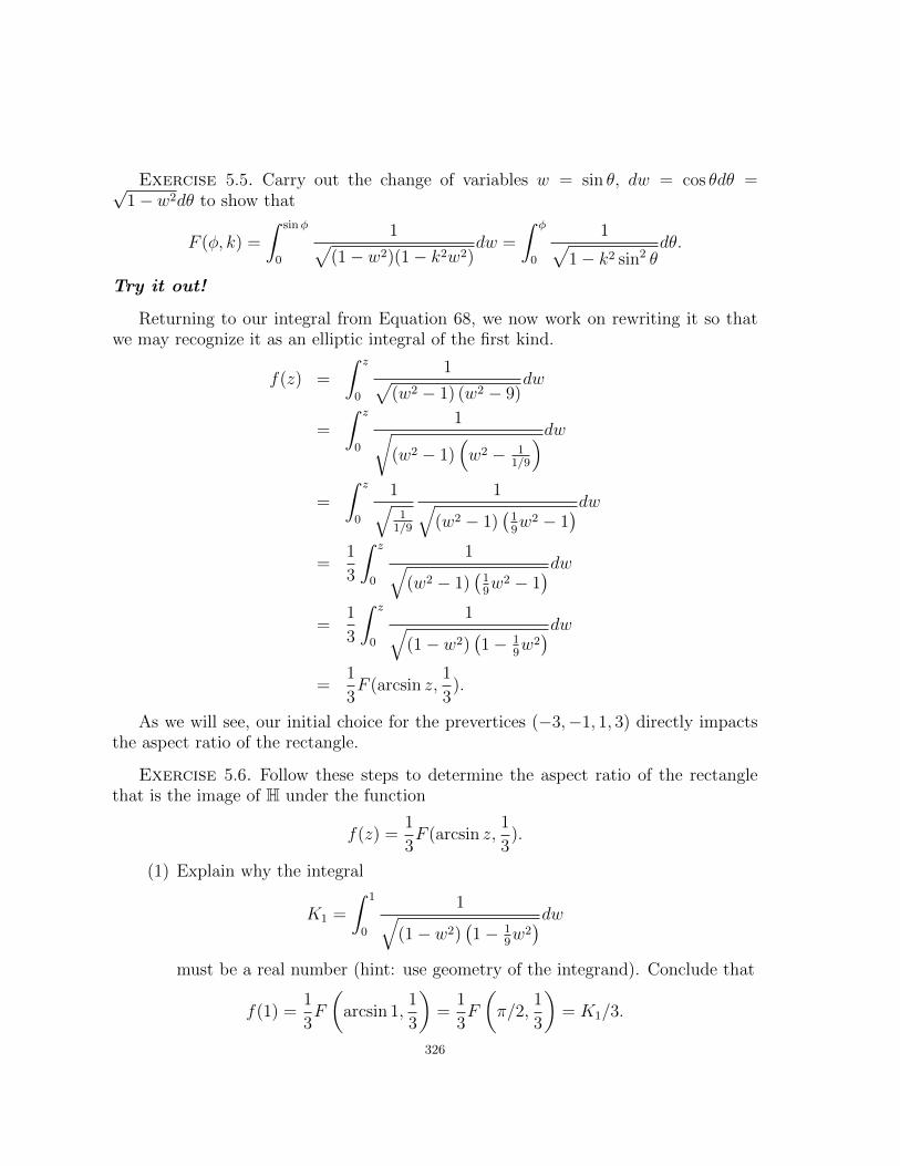
In the following example, we will apply the Schwarz-Christoffel formula to mapthe upper half-plane onto a rectangle. We will make a somewhat arbitrary choice ofprevertices, and then evaluate the resulting integral to determine the target rectangle.In computing the integral, we come across a first example of a special function, andfind that we need to learn some of the basics of elliptic integrals. We will find that justas the prevertices were arbitrarily chosen, so are the sidelengths of our target rectangle.
Example 5.3. In this example, we map the upper half-plane H onto a rectangle.We will choose the prevertices x1 = −3, x2 = −1, x3 = 1, and x4 = 3. Since our targetimage is a rectangle, all of the exterior angles are π/2, so each βi = 1/2. Using equation67, we find that
f(z) = A1
∫ z
0
1
(w − 1)1/2 (w − 3)1/2 (w + 1)1/2 (w + 3)1/2dw + A2, z ∈ H.
The constant A1 allows us to scale and rotate the image of H, and A2 allows for atranslation. By chosing A1 = 1 and A2 = 0 we simplify to
(68) f(z) =
∫ z
0
1√(w2 − 1) (w2 − 9)
dw.
This choice of constants does not affect the aspect ratio (ratio of adjacent sides)of the resulting rectangle. However the integral cannot be evaluated using techniquesin standard calculus texts. Instead it is a special function known as an elliptic integral(of the first kind, with parameter k = 1
3).
Definition 5.4. An elliptic integral of the first kind is an integral of the form
F (φ, k) =
∫ sinφ
0
1√(1− w2)(1− k2w2)
dw.
An alternate form is F (φ, k) =∫ φ
01√
1−k2 sin2 θdθ.
The two integrals in Definition 5.4 are identical after the change of variablesw = sin θ, dw = cos θdθ =
√1− w2dθ which connects them. (Technology note: The
computer algebra system Mathematica uses the alternate form, representing the inte-gral by EllipticF[φ,m], where m = k2.)
325
Exercise 5.5. Carry out the change of variables w = sin θ, dw = cos θdθ =√1− w2dθ to show that
F (φ, k) =
∫ sinφ
0
1√(1− w2)(1− k2w2)
dw =
∫ φ
0
1√1− k2 sin2 θ
dθ.
Try it out!
Returning to our integral from Equation 68, we now work on rewriting it so thatwe may recognize it as an elliptic integral of the first kind.
f(z) =
∫ z
0
1√(w2 − 1) (w2 − 9)
dw
=
∫ z
0
1√(w2 − 1)
(w2 − 1
1/9
)dw=
∫ z
0
1√1
1/9
1√(w2 − 1)
(19w2 − 1
)dw=
1
3
∫ z
0
1√(w2 − 1)
(19w2 − 1
)dw=
1
3
∫ z
0
1√(1− w2)
(1− 1
9w2)dw
=1
3F (arcsin z,
1
3).
As we will see, our initial choice for the prevertices (−3,−1, 1, 3) directly impactsthe aspect ratio of the rectangle.
Exercise 5.6. Follow these steps to determine the aspect ratio of the rectanglethat is the image of H under the function
f(z) =1
3F (arcsin z,
1
3).
(1) Explain why the integral
K1 =
∫ 1
0
1√(1− w2)
(1− 1
9w2)dw
must be a real number (hint: use geometry of the integrand). Conclude that
f(1) =1
3F
(arcsin 1,
1
3
)=
1
3F
(π/2,
1
3
)= K1/3.
326

By symmetry, show that f(−1) = −K1/3. Thus the length of one side of therectangle is 2|K1|/3.
(2) Determine that since f(3) is the next vertex of the target rectangle (movingcounterclockwise), and f(3) = f(1) + iK2 where K2 is some real constant.Combine this with the fact that
f(3) =1
3F
(arcsin 3,
1
3
)to show that iK2 = 1
3
(F (arcsin 3, 1
3)− F (π/2, 1
3)). The choice of sign for
K2 could be either positive or negative, depending on our choice of√−1.
For consistency with our choice of angles, K2 should be positive (note thatMathematica uses the “wrong” branch of the square root for this function onthe real axis).
(3) Combine the findings above to determine that the aspect ratio of the rectangleis
2F(π/2, 1
3
)F(arcsin 3, 1
3
)− F
(π/2, 1
3
) ≈ 1.279...
Figure 5.2. Portion of upper half-plane (left) and portion of targetrectangle (right) to which it maps under the function of Exercise 5.3.
The mapping for Example 5.3 is illustrated in Figure 5.2. Only a portion of theupper half-plane and its image are shown. This explains why the target rectangle isincompletely filled in the upper central area. However we can see that the aspect ratiois at least approximately the same as the one we calculated.
Small Project 5.7. Rework Example 5.3 for a more general situation. Use theprevertices x1 = −λ, x2 = −1, x3 = 1, and x4 = λ, where λ > 1. You can findan equation involving λ as a variable that, chosen correctly, would force the targetrectangle to be a square. To make the target rectangle a square, you find that λis part of an equation that cannot be explicitly solved, and must be approximatednumerically. This is a standard problem in some introductory complex analysis books(see for instance example 22 of section 14, [19]).
One observation we can make based on this example is that while it is straight-forward to write down a mapping function that has the correct angles, there is no
327

simple way to prescribe the side-lengths. Also, there are only a few rare cases whenour integral can be expressed in terms of elementary functions, and in general it is noteasy to evaluate. In order to find and evaluate specific Schwarz-Christoffel mappings,it is usually helpful to use symmetry of the target polygon (and of the prevertices) tosimplify the computations.
A further simplification to the Schwarz-Christoffel formula that is frequently em-ployed is to set one of the prevertices to be ∞, which effectively removes one factorfrom the denominator of the Schwarz-Christoffel formula. An example where thissimplification is helpful is in mapping onto a triangle.
We note here that there is no guarantee that the Schwarz-Christoffel formula willresult in a univalent function (see [9]). The only thing we can say for sure is that a mapfrom the upper half plane to a simply connected polygonal domain that is conformalMUST take the form of equation 67 for some choice of constants and prevertices (formore detail, see [3]).
In Exercise 5.6, we made use of symmetry by choosing the prevertices to be ±1 and±3. This symmetry simplified our calculations of the rectangle’s vertices. However weunable to easily find a mapping onto a square. In mapping onto a square, or ontoany regular polygon, it makes sense to adapt the Schwarz-Christoffel formula to mapthe unit disk to the polygon, using symmetrically placed points on the unit circle inplace of the xi in our existing formula. This can be accomplished by precomposingour mapping function found with Equation 67 with a Mobius transformation from theunit disk to the upper half-plane discussed in Exercise 5.1.
In addition to the problem of prescibing the lengths of the sides of the target poly-gon, a further problem arises with this approach for target polygons more complicatedthan a rectangle. Typically we will produce an integral that cannot be evaluated,even with special functions. These two issues are nicely resolved if we instead obtaina Schwarz-Christoffel formula that maps the unit disk directly to the target polygonand with the preimages of the vertices falling on the unit circle. These points canbe chosen, for example, to be roots of unity to give some symmetry in the integral.To obtain this formula we carry out a change of variables that maps the disk to theupper half-plane, using the map defined in Exercise 5.1. Interestingly, the transformedintegral formula is of exactly the same form.
Exercise 5.8. Set w = φ (z) = i1+z1−z which maps the disk in the z plane to the
upper half w-plane (see Exercise 5.1). Show that the Schwarz-Christoffel formularetains the same form as equation 67. Try it out!
The Schwarz-Christoffel map that we will use on the unit disk is then
f(z) = C1
∫ z
0
1
(w − ζ1)β1(w − ζ2)β2 · · · (w − ζn)βndw + C2, z ∈ D,
where βiπ is the exterior angle of the ith vertex of the target polygon, and the pre-images ζi of the vertices are on the unit circle. Here we use ζi instead of xi to emphasize
328
that the prevertices are not on the real axis. As with Equation 67, the complexconstants C1 and C2 with C1 6= 0 rotate, resize and translate the polygon.
With our original Schwarz-Christoffel formula from the upper half plane, it is notat all obvious how we could obtain a map onto a regular polygon. However, we canexploit the symmetries of the roots of unity by choosing ζi to be the symmetricallyplaced nth roots of unity corresponding to symmetrically placed vertices in the targetpolygon. Consequently, all side lengths of the target polygon will be equal.
Example 5.9. We obtain the Schwarz-Christoffel map onto a regular n-gon. Theexterior angles of a regular n-gon are 2π/n, so βi = 2/n.∫ z
0
1
(w − ζ1)β1(w − ζ2)β2 · · · (w − ζn)βndw =
∫ z
0
1
[(w − ζ1)(w − ζ2) · · · (w − ζn)]2/ndw
Suppose that the ζi are the nth roots of unity. Now we can use the fact that
n∏i=1
(w − ζi) = wn − 1
to simplify to∫ z
01
(wn−1)2/ndw. By factoring out (−1)2/n we can adjust the multiplicative
constant and chose our mapping function
(69) f (z) = (−1)−2/n
∫ z
0
1
(wn − 1)2/ndw =
∫ z
0
1
(1− wn)2/ndw.
Here f has been defined from the Schwarz-Christoffel formula with choices of constant
C1 = (−1)−2/n (which rotates the figure by 4π/n radians) and C2 = 0. This lastformula cannot be evaluated using the usual methods from calculus, but can be readilyevaluated using hypergeometric functions.
5.2.1. Basic Facts about Hypergeometric Functions. The integral in thelast example cannot be expressed in terms of elementary functions, but can be easilyevaluated and plotted using a computer algebra system by using some basic factsabout some special power series known as hypergeometric functions. Hypergeometricfunctions, besides their many other applications, can be used to evaluate the integralsobtained above. A geometric series is a power series in which ratios of successive termsare constant. Generalizing this, for a hypergeometric series ratios of successive termsare rational functions of the index rather than just constants. Here we will make use ofthe most widely utilized hypergeometric functions–the so-called “two F ones,” wherethe rational function has numerator and denominator of the second order.
Definition 5.10. The hypergeometric function 2F1(a, b; c; z) is the power series
2F1 (a, b; c; z) =∞∑n=0
(a)n(b)n(c)n
zn
n!,
329
where a, b and c ∈ C and
(x)n = x(x+ 1) · · · (x+ n− 1)
is the shifted factorial, or Pochhammer symbol.
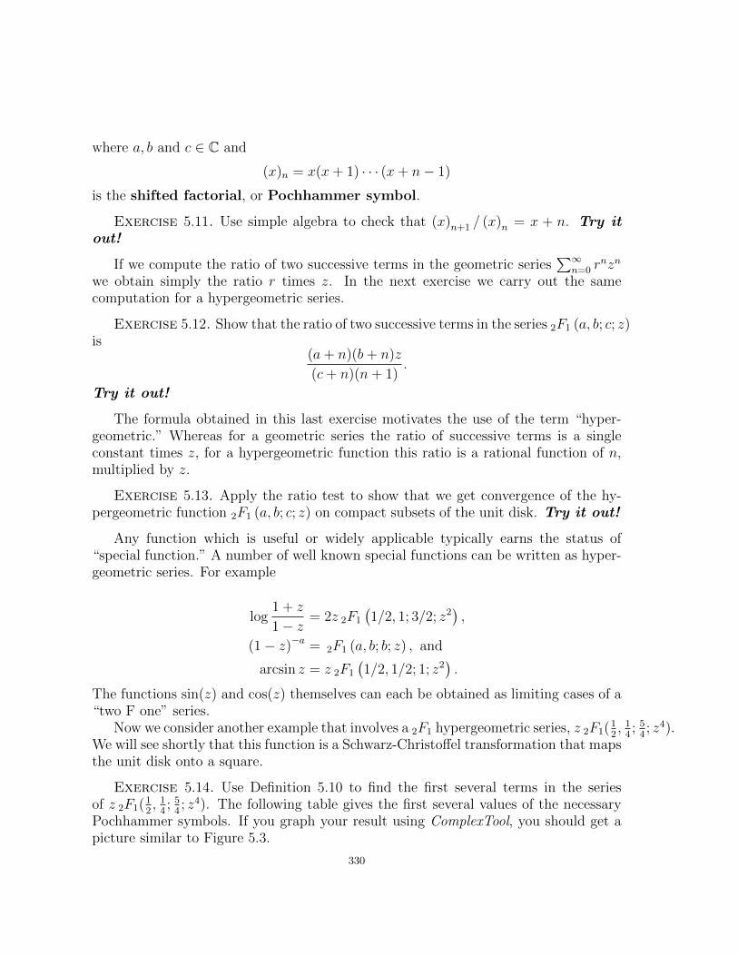
Exercise 5.11. Use simple algebra to check that (x)n+1 / (x)n = x + n. Try itout!
If we compute the ratio of two successive terms in the geometric series∑∞
n=0 rnzn
we obtain simply the ratio r times z. In the next exercise we carry out the samecomputation for a hypergeometric series.
Exercise 5.12. Show that the ratio of two successive terms in the series 2F1 (a, b; c; z)is
(a+ n)(b+ n)z
(c+ n)(n+ 1).
Try it out!
The formula obtained in this last exercise motivates the use of the term “hyper-geometric.” Whereas for a geometric series the ratio of successive terms is a singleconstant times z, for a hypergeometric function this ratio is a rational function of n,multiplied by z.
Exercise 5.13. Apply the ratio test to show that we get convergence of the hy-pergeometric function 2F1 (a, b; c; z) on compact subsets of the unit disk. Try it out!
Any function which is useful or widely applicable typically earns the status of“special function.” A number of well known special functions can be written as hyper-geometric series. For example
log1 + z
1− z = 2z 2F1
(1/2, 1; 3/2; z2
),
(1− z)−a = 2F1 (a, b; b; z) , and
arcsin z = z 2F1
(1/2, 1/2; 1; z2
).
The functions sin(z) and cos(z) themselves can each be obtained as limiting cases of a“two F one” series.
Now we consider another example that involves a 2F1 hypergeometric series, z 2F1(12, 1
4; 5
4; z4).
We will see shortly that this function is a Schwarz-Christoffel transformation that mapsthe unit disk onto a square.
Exercise 5.14. Use Definition 5.10 to find the first several terms in the seriesof z 2F1(1
2, 1
4; 5
4; z4). The following table gives the first several values of the necessary
Pochhammer symbols. If you graph your result using ComplexTool, you should get apicture similar to Figure 5.3.
330
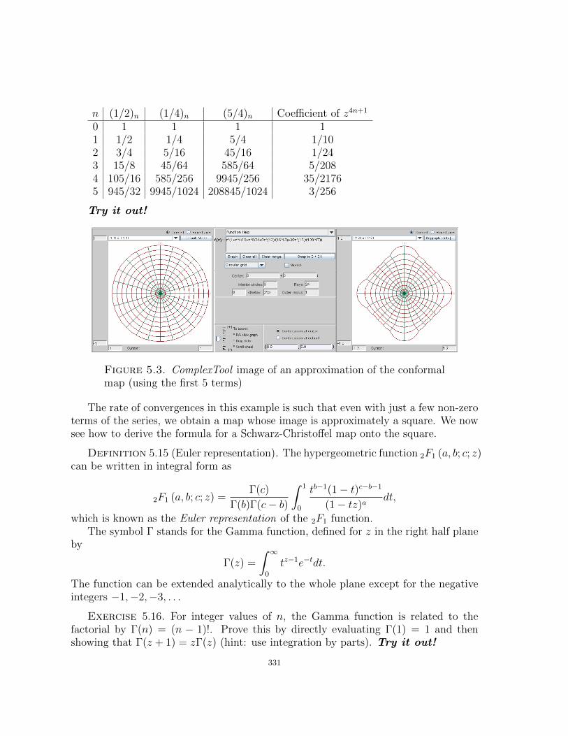
n (1/2)n (1/4)n (5/4)n Coefficient of z4n+1
0 1 1 1 11 1/2 1/4 5/4 1/102 3/4 5/16 45/16 1/243 15/8 45/64 585/64 5/2084 105/16 585/256 9945/256 35/21765 945/32 9945/1024 208845/1024 3/256
Try it out!
Figure 5.3. ComplexTool image of an approximation of the conformalmap (using the first 5 terms)
The rate of convergences in this example is such that even with just a few non-zeroterms of the series, we obtain a map whose image is approximately a square. We nowsee how to derive the formula for a Schwarz-Christoffel map onto the square.
Definition 5.15 (Euler representation). The hypergeometric function 2F1 (a, b; c; z)can be written in integral form as
2F1 (a, b; c; z) =Γ(c)
Γ(b)Γ(c− b)
∫ 1
0
tb−1(1− t)c−b−1
(1− tz)adt,
which is known as the Euler representation of the 2F1 function.The symbol Γ stands for the Gamma function, defined for z in the right half plane
by
Γ(z) =
∫ ∞0
tz−1e−tdt.
The function can be extended analytically to the whole plane except for the negativeintegers −1,−2,−3, . . .
Exercise 5.16. For integer values of n, the Gamma function is related to thefactorial by Γ(n) = (n − 1)!. Prove this by directly evaluating Γ(1) = 1 and thenshowing that Γ(z + 1) = zΓ(z) (hint: use integration by parts). Try it out!
331
Exercise 5.17. In this exercise, you will show that Definitions 5.10 and 5.15 areequivalent.
(1) Expand the factor (1− tz)−a with the binomial theorem as a power series toobtain
(1− tz)−a =∞∑n=0
(a)nn!
tnzn.
(2) Use the formula (see [14] Theorem 7, p. 19 for a proof)
Γ (p) Γ (q) = Γ (p+ q) ·∫ 1
0
tp−1 (1− t)q−1 dt
(where p and q have positive real parts) to show∫ 1
0
tn+b−1(1− t)c−b−1dt =Γ (b+ n) Γ (c− b)
Γ (c+ n).
The integral on the right is also an important special function known as thebeta function in the variables p and q.
(3) Show
(b)n(c)n
=Γ (c)
Γ (b) Γ (c− b)Γ (b+ n) Γ (c− b)
Γ (c+ n).
(4) Put the previous facts together to obtain the required formula. Substitute thepower series for the denominator term, and then interchange summation andintegral, to show that∫ 1
0
tb−1(1− t)c−b−1
(1− tz)adt =
Γ (b) Γ (c− b)Γ (c)
2F1 (a, b; c; z) .
Try it out!
It takes a little work to establish the relationship of the beta function with theGamma function used in part (2). For an excellent exposition of this fact and anintroduction to special functions in general, see [14].
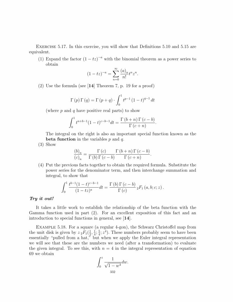
Example 5.18. For a square (a regular 4-gon), the Schwarz Christoffel map fromthe unit disk is given by z 2F1(1
2, 1
4; 5
4; z4). These numbers probably seem to have been
essentially “pulled from a hat,” but when we apply the Euler integral representationwe will see that these are the numbers we need (after a transformation) to evaluatethe given integral. To see this, with n = 4 in the integral representation of equation69 we obtain ∫ z
0
1√1− w4
dw.
332
Let a = 1/4, b = 1/2, and c = 5/4. We use the Euler integral representation for
2F1 (a, b; c; z) to evaluate
2F1
(1/2, 1/4; 5/4; z4
)=
Γ(5/4)
Γ(1/4)Γ(1)
∫ 1
0
t−3/4(1− t)0
(1− tz4)1/2dt
= 1/4
∫ 1
0
1
t3/41√
1− tz4dt.
Now change variables by letting w4 = tz4 (so t = (w4/z4)) and 4w3dw = z4dt. Then
2F1
(1/2, 1/4; 5/4; z4
)= 1/4
∫ z
0
z3
w3
1√1− w4
4w3dw
z4
=1
z
∫ z
0
1√1− w4
dw.
Thus
f (z) =
∫ z
0
1√1− w4
dw = z 2F1
(1/2, 1/4; 5/4; z4
).
Figure 5.4. Unit disk (left) and target square (right) to which it mapsunder the function of Exercise 5.18.
Contrast the map in Figure 5.4, where the domain is the (bounded) unit disk, withthe earlier map onto a rectangle in Figure 5.2. One advantage with the disk map isthat we can see the entire mapping domain and the entire target square is filled. Notealso the rotational and reflectional symmetry obtained by using nth roots of unity onthe unit circle as prevertices.
Exercise 5.19. Show that the conformal map from the disk onto the regular n-gonis (up to rotations, translations and scalings) given by z 2F1 (2/n, 1/n; (n+ 1) /n; zn) .Try it out!
We describe another situation where this technique of integration can be useful, forreaders who have worked through Chapters 2 or 4. In Chapter 4, Section 4.5 discusses
333
the shear construction, and in Chapter 2, Section 2.6 the shear construction and itsrelationship to minimal surfaces is discussed.
Small Project 5.20. Define a non-convex 6-sided polygon P with β1 = β4 =−1/3 and β2 = β3 = β5 = β6 = 2/3. (Draw this polygon!) Find a representation forthe Schwarz-Christoffel transformation that maps the unit disk D onto P , with theprevertices ζi being the 6th roots of unity. It works well if ζ1 = 1 and ζ4 = −1, withthe other 6th roots of unity going in order counterclockwise around the circle. Verifythat the analytic function f(z) : P → D is given by
f(z) = z 2F1
(2
3,1
6;7
6; z6
)− z3
32F1
(2
3,1
2;3
2; z6
).
Now, in the language of Chapter 4, let h(z)− g(z) be the function given above as
f(z) and let the dilatation ω(z) = z2. Find the harmonic function h(z) + g(z). Verifythat by using
h(z) = z 2F1
(2
3,1
6;7
6; z6
)and
g(z) =z3
32F1
(2
3,1
2;3
2; z6
),
it is indeed true that ω(z) = h′
g′= z2. Use a computer algebra system to create a
picture of the image of D under the function h(z) + g(z).Furthermore, if you have studied Chapter 2, you can find the minimal surface that
lifts from this harmonic function. You should find that it is defined by
x1 = Re
(z 2F1
(2
3,1
6;7
6; z6
)+z3
32F1
(2
3,1
2;3
2; z6
))x2 = Im
(z 2F1
(2
3,1
6;7
6; z6
)− z3
32F1
(2
3,1
2;3
2; z6
))x3 = Im
(z2
2F1
(2
3,1
3;3
2; z6
)).
We now examine the conformal map onto a symmetric non-convex polygon inthe shape of a star. We intend in the next section to find harmonic maps onto thesame figure, and will find that while mappings onto polygons with convex corners arerelatively easy to construct, there is little or no supporting theory when non-convexcorners are involved.
Example 5.21. Suppose we want to map onto a (non-convex) m-pointed star, sothere are n = 2m vertices. The interior angles alternate between πα1 and πα2 whereα1 < 1 < α2 (so a “sharp point” of the star occurs at α1). Corresponding exteriorangles then alternate between a positive value β1 and a negative value β2 (assumingwe have a non-convex star).
334
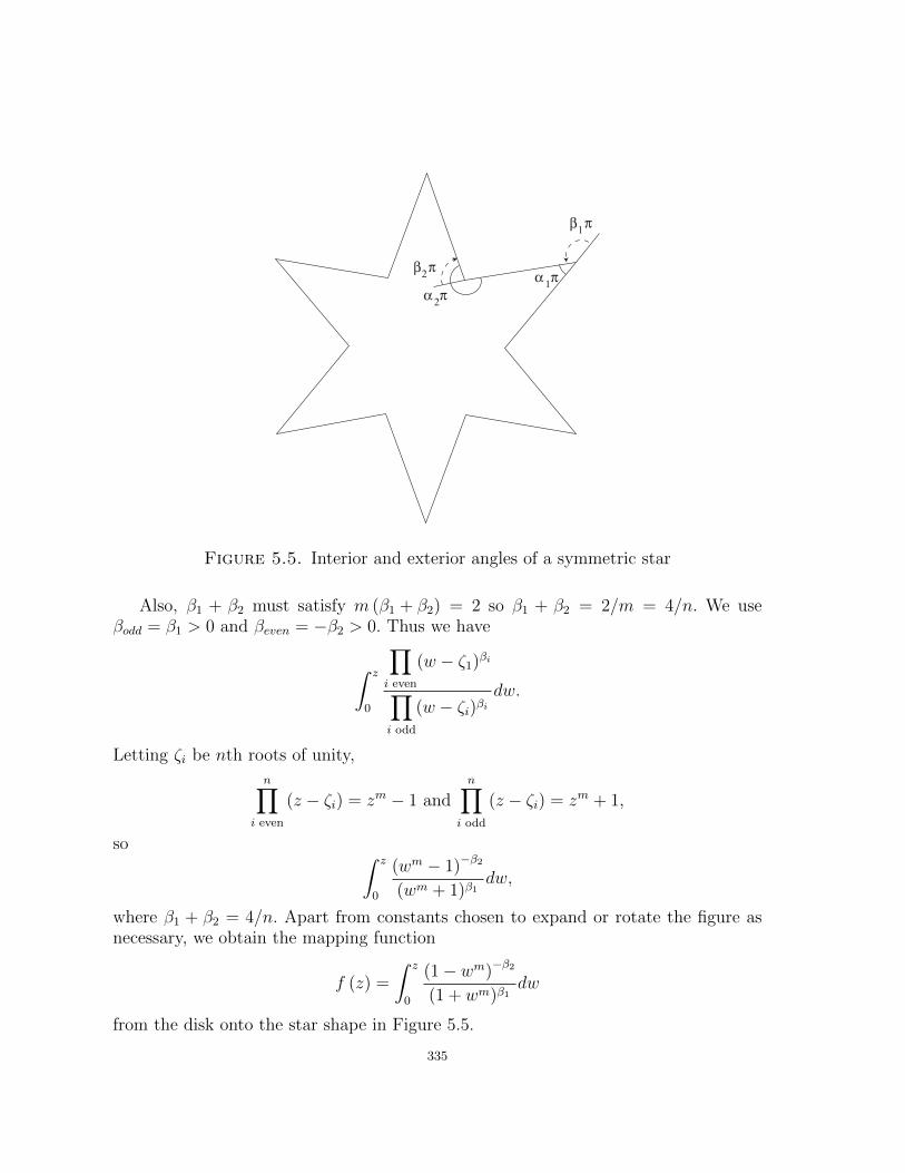
β π2
α π2
β π1
α π1
Figure 5.5. Interior and exterior angles of a symmetric star
Also, β1 + β2 must satisfy m (β1 + β2) = 2 so β1 + β2 = 2/m = 4/n. We useβodd = β1 > 0 and βeven = −β2 > 0. Thus we have
∫ z
0
∏i even
(w − ζ1)βi∏i odd
(w − ζi)βidw.
Letting ζi be nth roots of unity,
n∏i even
(z − ζi) = zm − 1 andn∏
i odd
(z − ζi) = zm + 1,
so ∫ z
0
(wm − 1)−β2
(wm + 1)β1dw,
where β1 + β2 = 4/n. Apart from constants chosen to expand or rotate the figure asnecessary, we obtain the mapping function
f (z) =
∫ z
0
(1− wm)−β2
(1 + wm)β1dw
from the disk onto the star shape in Figure 5.5.
335
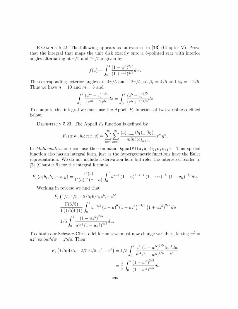
Example 5.22. The following appears as an exercise in [13] (Chapter V). Provethat the integral that maps the unit disk exactly onto a 5-pointed star with interiorangles alternating at π/5 and 7π/5 is given by
f(z) =
∫ z
0
(1− w5)2/5
(1 + w5)4/5dw.
The corresponding exterior angles are 4π/5 and −2π/5, so β1 = 4/5 and β2 = −2/5.Thus we have n = 10 and m = 5 and∫ z
0
(zm − 1)−β2
(zm + 1)β1dz =
∫ z
0
(z5 − 1)2/5
(z5 + 1)4/5dz
To compute this integral we must use the Appell F1 function of two variables definedbelow.
Definition 5.23. The Appell F1 function is defined by
F1 (a; b1, b2; c;x, y) =∞∑n=0
∞∑m=0
(a)n+m (b1)m (b2)nm!n! (c)n+m
xmyn,
In Mathematica one can use the command AppelF1(a,b1,b2,c,x,y). This specialfunction also has an integral form, just as the hypergeometric functions have the Eulerrepresentation. We do not include a derivation here but refer the interested reader to[2] (Chapter 9) for the integral formula
F1 (a; b1, b2; c;x, y) =Γ (c)
Γ (a) Γ (c− a)
∫ 1
0
ua−1 (1− u)c−a−1 (1− ux)−b1 (1− uy)−b2 du.
Working in reverse we find that
F1
(1/5; 4/5,−2/5; 6/5; z5,−z5
)=
Γ(6/5)
Γ(1/5)Γ(1)
∫ 1
0
u−4/5 (1− u)0 (1− uz5)−4/5 (
1 + uz5)2/5
du
= 1/5
∫ 1
0
(1− uz5)2/5
u4/5 (1 + uz5)4/5du.
To obtain our Schwarz-Christoffel formula we must now change variables, letting w5 =uz5 so 5w4dw = z5du. Then
F1
(1/5; 4/5,−2/5; 6/5; z5,−z5
)= 1/5
∫ z
0
z4
w4
(1− w5)2/5
(1 + w5)4/5
5w4dw
z5
=1
z
∫ z
0
(1− w5)2/5
(1 + w5)4/5dw
336

Thus
f (z) =
∫ z
0
(1− w5)2/5
(1 + w5)4/5dw = z F1
(1/5; 4/5,−2/5; 6/5; z5,−z5
)and the mapping function is shown in Figure 5.6.
Figure 5.6. Image of the conformal map of the unit disk onto the 5-pointed star
Exercise 5.24. Show that the conformal map from the disk onto the m pointedstar with exterior angle β1 > 0, and β2 = 2/m − β1 (up to rotations, translationsand scalings) is given by z F1 (1/n; β1, β2, (n+ 1) /n; zn,−zn) where F1 is the AppellF1 function. Try it out!
5.3. The Poisson Integral Formula
While the Schwarz-Christoffel formula gives analytic and thus angle-preserving(conformal) functions from D to any polygon, we can see that it often starts withan integral that requires advanced mathematics to evaluate. If our goal is not nec-essarily an analytic function, we could work with the Poisson integral formula. Thisdoes not give us an analytic function, but instead, a harmonic function from the unitdisk to the target domain. We first recall the definition of a harmonic function.
Definition 5.25. A real-valued function u(x, y) is harmonic provided that
uxx + uyy = 0.
337
A complex-valued function f(z) = f(x+ iy) = u(x, y) + iv(x, y) is harmonic if both uand v are harmonic.
The definition of a complex-valued harmonic function does not require that thefunctions u and v be harmonic conjugates, so while all analytic functions are harmonic,a complex-valued harmonic function is not necessarily analytic. In fact, the functionswe work with for the rest of the chapter will not be analytic, and thus not conformal.
You may be familiar with the Poisson integral formula as a way of constructing areal-valued harmonic function that satisfies certain boundary conditions. For example,if the boundary conditions give the temperature of the boundary of a perfectly insulatedplate, then the harmonic function gives the steady-state temperature of the interiorof the plate. Another application is to find electrostatic potential given boundaryconditions. A brief summary of that procedure is given here. For more detaileddiscussion, consult [15] or [20].
Theorem 5.26 (Poisson Integral Formula). Let the complex valued function f(eiθ)be piecewise continuous and bounded for θ in [0, 2π] . Then the function f (z) definedby
(70) f(z) =1
2π
∫ 2π
0
1− |z|2|eit − z|2 f(eit)dt
is the unique harmonic function in the unit disk that satisfies the boundary condition
limr→1
f(reiθ) = f(eiθ)
for all θ where f is continuous.
Here, we present the proof in the special case where the boundary function f(eiθ)is the real part of a function that is analytic on a disk with radius larger than 1. Thisproof can be found in any standard complex analysis textbook, for example, [10] or[15]. The interested reader may find the full result in Chapter 6 of [?] and Chapter 8of [10].
Proof. (Special Case) First observe that Cauchy’s integral formula tells us thatif we have a function f(z) that is analytic inside and on the circle |z| = R, then, for|z| < R,
(71) f(z) =1
2πi
∫|ζ|=R
f(ζ)
ζ − zdζ.
Here we are using the Greek letter zeta (ζ) as the variable of integration in theintegral. In the discussion that follows here, we will be thinking about evaluating thefunction f(z) at some fixed value of z, so the variable under consideration is now ζ.We also observe (for reasons that will become obvious in a few sentences) that for
fixed z, with |z| < 1, the functionf(ζ) z
1− ζ z is analytic in the variable ζ on and inside
338
|ζ| < 1, since the denominator is non-zero. (Exercise for the reader: Think about whythe denominator is non-zero.) Thus, by the Cauchy Integral Theorem, we know that
(72)1
2πi
∫|ζ|=1
f(ζ) z
1− ζ z = 0.
Combining Equations 71 and 72, we see that
f(z) =1
2πi
∫|ζ|=1
f(ζ)
ζ − zdζ + 0
=1
2πi
∫|ζ|=1
(f(ζ)
ζ − z +f(ζ) z
1− ζ z
)dζ
=1
2πi
∫|ζ|=1
1− ζ z + z(ζ − z)
(ζ − z)(1− ζ z)f(ζ)dζ
=1
2πi
∫|ζ|=1
1− |z|2(ζ − z)(1− ζ z)
f(ζ)dζ.
Now we parameterize the circle |ζ| = 1 by ζ(t) = eit, giving dζ = ieitdt and
f(z) =1
2πi
∫ 2π
0
1− |z|2(eit − z)(1− eit z)
f(eit)ieitdt
=1− |z|2
2π
∫ 2π
0
1
(eit − z)eit(e−it − z)f(eit)eitdt
=1− |z|2
2π
∫ 2π
0
f(eit)
(eit − z)(e−it − z)dt.
Taking the real part of both sides of the equation gives us a harmonic function (sincethe real part of an analytic function is harmonic), and also yields Equation 70.
Exercise 5.27. Verify that the “Poisson kernel,”1− |z|2|eit − z|2 , can be rewritten as
Re
(eit + z
eit − z
)= Re
(1 + ze−it
1− ze−it)
. Try it out!
The integral in Equation 70 is, in general, very difficult to integrate. However, ifthere is an arc on which the function f(eit) is constant, then the integration is easy todo.
Exercise 5.28. Verify that(73)1
2π
∫ b
a
K Re
(eit + z
eit − z
)dt = K
b− a2π
+K
πarg
(1− ze−ib1− ze−ia
)=K
π
[arg
(eib − zeia − z
)− b− a
2
].
339
Helpful hints: Swap the order of integration and taking the real part of a function.The algebraic identity 1+w
1−w = 1 + 2w1−w will be helpful.
Try it out!
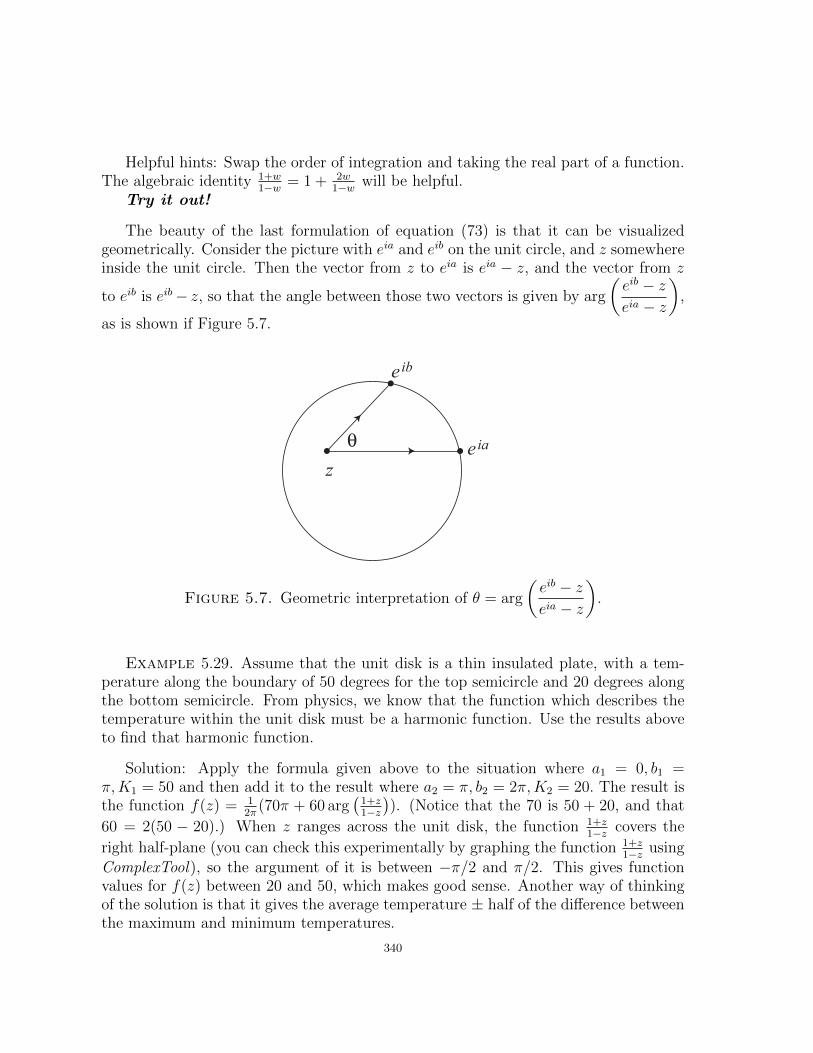
The beauty of the last formulation of equation (73) is that it can be visualizedgeometrically. Consider the picture with eia and eib on the unit circle, and z somewhereinside the unit circle. Then the vector from z to eia is eia − z, and the vector from z
to eib is eib− z, so that the angle between those two vectors is given by arg
(eib − zeia − z
),
as is shown if Figure 5.7.
eiaz
eib
θ
Figure 5.7. Geometric interpretation of θ = arg
(eib − zeia − z
).
Example 5.29. Assume that the unit disk is a thin insulated plate, with a tem-perature along the boundary of 50 degrees for the top semicircle and 20 degrees alongthe bottom semicircle. From physics, we know that the function which describes thetemperature within the unit disk must be a harmonic function. Use the results aboveto find that harmonic function.
Solution: Apply the formula given above to the situation where a1 = 0, b1 =π,K1 = 50 and then add it to the result where a2 = π, b2 = 2π,K2 = 20. The result isthe function f(z) = 1
2π(70π + 60 arg
(1+z1−z
)). (Notice that the 70 is 50 + 20, and that
60 = 2(50 − 20).) When z ranges across the unit disk, the function 1+z1−z covers the
right half-plane (you can check this experimentally by graphing the function 1+z1−z using
ComplexTool), so the argument of it is between −π/2 and π/2. This gives functionvalues for f(z) between 20 and 50, which makes good sense. Another way of thinkingof the solution is that it gives the average temperature ± half of the difference betweenthe maximum and minimum temperatures.
340

Exercise 5.30. Referring to f(z) = 12π
(70π + 60 arg(
1+z1−z
)) in the solution to
Example 5.29, find f(0), f(i/2) and f(−i/2). Do your answers make sense?
Using the result of Exercise 5.28, we can see that computing the Poisson integralformula for a piecewise constant boundary is particularly simple. Many applications ofthe Poisson integral formula come from having the boundary correspondence remainconstant on arcs of the unit circle.
Most introductory analysis books give the Poisson integral formula for real-valuedf(eiθ). It can also be applied to create a harmonic function for complex-valued f(eiθ),but the univalence of the harmonic function is not at all apparent. Let’s first explorewhat could happen if we try to use the Poisson integral formula with complex boundaryvalues.
Example 5.31. The simplest example of this is obtained by letting the first thirdof the unit circle (that is, the arc from 0 to ei2π/3) map to 1, the next third to ei2π/3
and the last third to ei4π/3. Let’s work through the details of this integration, workingfrom equation (73). We compute
f(z) =1
2π
((2π
3− 0) + 2 arg
(1− ze−i2π/3
1− ze0
)+ei2π/3(
4π
3− 2π
3) + 2ei2π/3 arg
(1− ze−i4π/31− ze−i2π/3
)+ei4π/3(2π − 4π
3) + 2ei4π/3 arg
(1− ze−2πi
1− ze−i4π/3))
=2π
3(2π)
(1 + ei2π/3 + ei4π/3
)+
1
π
(arg
(1− ze−i2π/3
1− ze0
)+ ei2π/3 arg
(1− ze−i4π/31− ze−i2π/3
)+ ei4π/3 arg
(1− ze−2πi
1− ze−i4π/3))
= 0 +1
π
(arg
(1− ze−i2π/3
1− z
)+ ei2π/3 arg
(1− ze−i4π/31− ze−i2π/3
)+ ei4π/3 arg
(1− z
1− ze−i4π/3))
.
Figure 5.8 shows the image of the unit disk as graphed in ComplexTool. Notice thatit appears to be one-to-one on the interior of the unit disk. It certainly is not one-to-oneon the boundary! (Entering this formula into ComplexTool is a bit unwieldy, so thisfunction is one of the Pre-defined functions, the one called Harmonic Triangle.We will soon use the PolyTool applet, as described on the next page, to graph othersimilar functions.)
Exercise 5.32. Find a general formula that maps the unit disk harmonically tothe interior of a convex regular n-gon. Try it out!
341

Figure 5.8. ComplexTool image of the harmonic function mapping tothe triangle
Small Project 5.33. Refer to Chapter 4 and its discussion of the shear construc-tion. Find the pre-shears of the polygonal mappings in exercise 5.32. In other words,what analytic function do you shear to get that polygonal function? A good first stepis to determine the dilatation of this function. See [4] for more details.
Exercise 5.34. For a non-convex example, consider the function that maps quar-ters of the unit circle to the four vertices 1, i,−1, i
2. Verify that this function is
3i
8+
1
π
(arg
(1 + iz
1− z
)+ i arg
(1 + z
1 + iz
)− arg
(1− iz1 + z
)+i
2arg
(1− z1− iz
)).
When we graph this function in ComplexTool, we notice that it appears to NOT beone-to-one. Furthermore, f(0) = 3i
8, so that the image of D is not the interior of the
polygon. This function is another one of the Pre-defined functions in ComplexTool.Try it out!
Figure 5.9. The PolyTool Applet
At this point, you should start using the PolyTool applet. In this applet, youcan specify which arcs of the unit circle will map to which points in the range, and
342

the applet will compute and graph the harmonic function defined by extending thatboundary correspondence to a function on D. When you first open this applet, yousee a circle on the left and a blank screen on the right. You can create a harmonicfunction that maps portions of the boundary of the circle to vertices of a polygon inone of two ways. First, you can click on the unit circle in the left panel to denote anarc endpoint, and continue choosing arc endpoints there, and then choose the targetvertices by clicking in the right graph. (Note that as you click, text boxes in between thepanels fill with information about where you clicked.) Once you have the boundarycorrespondence you want, click the Graph button. Alternatively, you can click thebutton that says Add to get text boxes for input. For example, to create the functionin Exercise 5.34, click Add, then fill in the first row of boxes for Arc 1: with 0 maps
to 1+0i. When you want another set of arcs, click Add again. Note that the Arc boxesdenote the starting point of the arc (i.e. for the arc from 0 to π/3, use 0 in the Arc
box). Continue filling, and when you are ready to compute the Poisson integral to getthe harmonic function, click the Graph button. Once you have a function graphed, youcan “drag” around either the arc endpoints (in the domain on the left) or the targetpoints (in the range on the right) and watch the function dynamically change.
Exploration 5.35. Are there ways of rearranging the boundary conditions tomake the function created in Exercise 5.34 univalent? For example, what if the bottomhalf of the unit circle gets mapped to i/2, and the top half of the unit circle is dividedinto thirds for the other three vertices? This isn’t univalent, but in some sense is closerto univalent than the mapping defined in Exercise 5.34. Is there a modification to bemade so that it is univalent? Try it out!
Exercise 5.36. This is an extension of Exploration 5.35. Sheil-Small [17] proved(by techniques other than those discussed so far) that the harmonic extension of theboundary correspondence below maps the unit disk univalently onto the desired shape:
arc from to maps to−i i ii −3/5 + 4i/5 −1
−3/5 + 4i/5 −3/5− 4i/5 i/2−3/5− 4i/5 −i 1
For this function, first convince yourself that it appears to be univalent, and thenfind the function f(z). Try it out!
We will be working a lot with harmonic functions that are extensions of a piecewiseconstant boundary correspondence, as in the example above. To have a framework forfuture discussions, we make the following formal definition.
Definition 5.37. Let eitk be a partition of ∂D, where t0 < t1 < . . . < tn =
t0 + 2π. Let f(eit) = vk for tk−1 < t < tk. We call the harmonic extension of this stepfunction (as defined by the Poisson integral formula) f(z).
343

Example 5.38. To better understand the definition, we demonstrate how the no-tation in Definition 5.37 is used for the function in Exercise 5.36. Since the arc from−i to i can be thought of as the arc along the unit circle from e−iπ/2 to e−iπ/2, we saythat t0 = −π/2 and t1 = π/2. These points map to the vertex at i, so v1 = i. The nextarc set is a little more difficult, because we need to find the angle t2 that goes withthe point in the plane z = −3
5+ 4
5i = eit2 . Unfortunately, we can only get a numeri-
cal estimate of the angle, found by π + arctan(
4/5−3/5
)= π + arctan (−4/3) ≈ 2.2143.
(We add π because the output of arctangent is always in the first or fourth quadrant,while the angle in question is in the second quadrant.) Thus we have t2 ≈ 2.2143and v2 = −1. Continuing this process, we have t3 ≈ 4.0689 and v3 = i/2. Then wefinish with t4 = 3π/2 and v4 = 1. Notice that as in the definition, t4 = t0 + 2π. Thenthe function f(z) from Definition 5.37 is the harmonic function that appears to beunivalent when graphed in PolyTool.
Exercise 5.39. Combine the result of Exercise 73 (on page 339) with Definition5.37 to show that the function f(z) in Definition 5.37 can be written
f(z) = v1
(t1 − t0
2π
)+v1
πarg
(1− ze−it11− ze−it0
)+v2
(t2 − t1
2π
)+v1
πarg
(1− ze−it21− ze−it1
)+ . . .+ vn
(tn − tn−1
2π
)+vnπ
arg
(1− ze−itn
1− ze−itn−1
).
Try it out!Since the Poisson integral formula gives rise to a harmonic function, we must learn
some of the basics of the theory of harmonic functions before proceeding too far.
5.4. Harmonic Function Theory
Chapter 4 gives a detailed explanation of harmonic functions, as does [5]. Much ofthat material will be helpful for our future investigations, so we repeat it here.
5.4.1. The Basics. Any harmonic function f can be written as f = h+ g, where
h and g are analytic functions. The analytic dilatation ω(z) = g′(z)h′(z)
is, in some sense, a
measure of how much the harmonic function does not preserve angles. A dilatation ofω(z) ≡ 0 means that the function is analytic, so must be conformal. A dilatation withmodulus near 1 indicates that the function distorts angles greatly. (For more intuitionabout the dilatation, read Section 4.6 of Chapter 4.) A result of Lewy states that aharmonic function has nonzero Jacobian (denoted Jf (z) = |h′|2 − |g′|2) if it is locallyunivalent. This result is in line with our understanding of the relationship betweenlocal univalence and a nonvanishing derivative for analytic functions.
344
Theorem 5.40 (Lewy’s Theorem). For a harmonic function f defined on a domainΩ, if f locally univalent in Ω, then Jf (z) 6= 0 for all z ∈ Ω.
Note that this is equivalent to Lewy’s Theorem in Chapter 4.A nice consequence of Lewy’s Theorem is that if a function is locally univalent in
Ω, then its analytic dilatation either satisfies |ω(z)| < 1 for all z ∈ Ω, or |ω(z)| > 1for all z ∈ Ω. In our work, we will only study functions that are locally univalentin some domain Ω and satisfy |ω(z)| < 1 for all z ∈ Ω. These functions are calledsense-preserving because they preserve the orientation of curves in Ω.
Exercise 5.41. Verify that the condition that Jf (z) 6= 0 is equivalent to |ω(z)| 6= 1,as long as h′(z) 6= 0. Conclude that a function that is locally univalent and sense-preserving must have Jf (z) > 0 and |ω(z)| < 1. Try it out!
Of particular interest in this setting is determining how to split up the argumentfunction (which is harmonic and sense-preserving) into h and g.
Exercise 5.42. Show that the function f(z) = K arg(z) has canonical decompo-
sition h(z) =1
2iK log(z) and g(z) =
1
2iK log(z). Try it out!
Another consequence of the canonical decomposition of a harmonic function is thatwe can write the analytic functions h and g defined in some domain Ω in terms of theirpower series expansions, centered at some z0 ∈ Ω, as
(74) f(z) = a0 +∞∑k=n
ak(z − z0)k + b0 +∞∑k=m
bk(z − z0)k.
If f is sense-preserving, then we necessarily have that either m > n or m = n with|bn| < |an|. In either case, when f is represented by Equation 74, we say that f has azero of order n at z0.
Exercise 5.43. In this exercise, we prove that the zeros of a sense-preservingharmonic function are isolated.
(a) Assume that f(z) is a sense-preserving locally univalent function with seriesexpansion as given in Equation 74. Show that if f(z0) = 0, there exists apositive δ and a function ψ such that, for 0 < |z − z0| < δ we can write
(75) f(z) = h(z) + g(z) = an(z − z0)n(1 + ψ(z))
where
ψ(z) =an+1
an(z − z0) +
an+2
an(z − z0)2 + · · ·+ bm(z − z0)m
1
an(z − z0)n+ · · · .
(b) Show that part (a) implies that |ψ(z)| < 1 for z sufficiently close to z0, sincem ≥ n and |bn/an| < 1 if m = n.
(c) Show that part (b) implies that the zeros of a sense-preserving harmonic func-tion are isolated, since f(z) 6= 0 near z0 (except, of course, at z0).
345
Try it out!
5.4.2. The Argument Principle.5.4.2.1. Analytic Argument Principle. The Argument Principle for analytic func-
tions gives a very nice way to describe the number of zeros and poles inside a contour.We take time to explore this topic, even though it is in many introductory complexanalysis courses, to emphasize the geometric nature of the result. We first provide aformal definition of a common phrase, the winding number of the image of a contourabout the origin.
Definition 5.44. The winding number of the image under f(z) of a simple closedcontour Γ about the origin is the net change in argument of f(z) as z traversesΓ in the positive (counterclockwise) direction, divided by 2π. It can be denoted by1
2π∆Γ arg f(z).
To explore the relationship between the winding number of the image of a contourabout the origin and the number of zeros and poles contained within that contour, dothe following exploration.
Exploration 5.45. Open ComplexTool. Change the Interior circles to 1 andthe Rays to 0. This will graph just the boundary of the circle of interest. As yougraph the following functions, examine the image of the circle “winds around,” orencloses, the origin. Count how many times the image of the circle winds around theorigin, making sure that you count the counterclockwise direction as positive and theclockwise direction as negative. If the image of the circle winds around the origin once,you know that there must be a zero of f(z) inside that circle. (Think about this lastsentence and make sure you understand it.)
• Graph f(z) = z2, using a circle of radius 1. Use the “Sketch” button and tracearound the circle in the domain to get a good feeling for how many times itsimage winds around the origin. You should already know the answer. (Anyother radius will work too. Why is that?)• Graph f(z) = z(z−0.3). Use circles of radius 0.2, 0.3 and 0.5. (You may have
to zoom in on the image of the circle of radius 0.2 to really understand whatit is doing.) If you want, you may check the Vary radius checkbox and usethe slider to change the radius of the circle.• Graph f(z) = z4 − 6z + 3. Use circles of radius 0.9, 1.5, 1.7, and 2.
• Graph f(z) = z4−6z+3z−1
, using circles of radius 0.9 and 1.5.
• Graph f(z) = z4−6z+3(z−1)2
, using circles of radius 0.9, 1.5 and 2.
• Go back through the previous 3 items, now changing the function while keepingthe radius fixed.• For all of the previous functions, find the locations of all of the zeros and poles,
paying particular attention to how far they are from the origin.• Make up your own function and do some more experiments.
346

Based on the explorations above, what is your connection between the winding numberof the image of a circle about the origin and the number of zeros and poles inside thecircle?
Try it out!
Theorem 5.46 (Argument Principle for Analytic Functions). Let C be a simpleclosed contour lying entirely within a domain D. Suppose f is analytic in D except ata finite number of poles inside C and that f(z) 6= 0 on C. Then
1
2πi
∮C
f ′(z)
f(z)dz = N0 −Np,
where N0 is the total number of zeros of f inside C and Np is the total number ofpoles of f inside C. In determining N0 and Np, zeros and poles are counted accordingto their order or multiplicity.
z2z1 0
Figure 5.10. A path around a branch cut
Before proving Theorem 5.46, we explore the connection between the winding num-
ber and the integral1
2πi
∮C
f ′(z)
f(z)dz. To see this connection, we start with a related
integral,∫ z2z1
f ′(z)f(z)
dz, where z1 and z2 are points very close to each other, but lying on
opposite sides of a branch cut of log f(z), and we take a “counterclockwise” path alongC from z1 to z2. (See Figure 5.10.) Now we do the following computation:∫ z2
z1
f ′(z)
f(z)dz = log f(z)|z2z1
= ln |f(z2)| − ln |f(z1)|+ i(arg(f(z2))− arg(f(z1))).
When we take the limit as z1 → z2, we get that ln |f(z2)| − ln |f(z1)| → 0 andi(arg(f(z2))− arg(f(z1)))→ 2πi · (winding number). (Think carefully about this laststatement and make sure you understand it.)
347
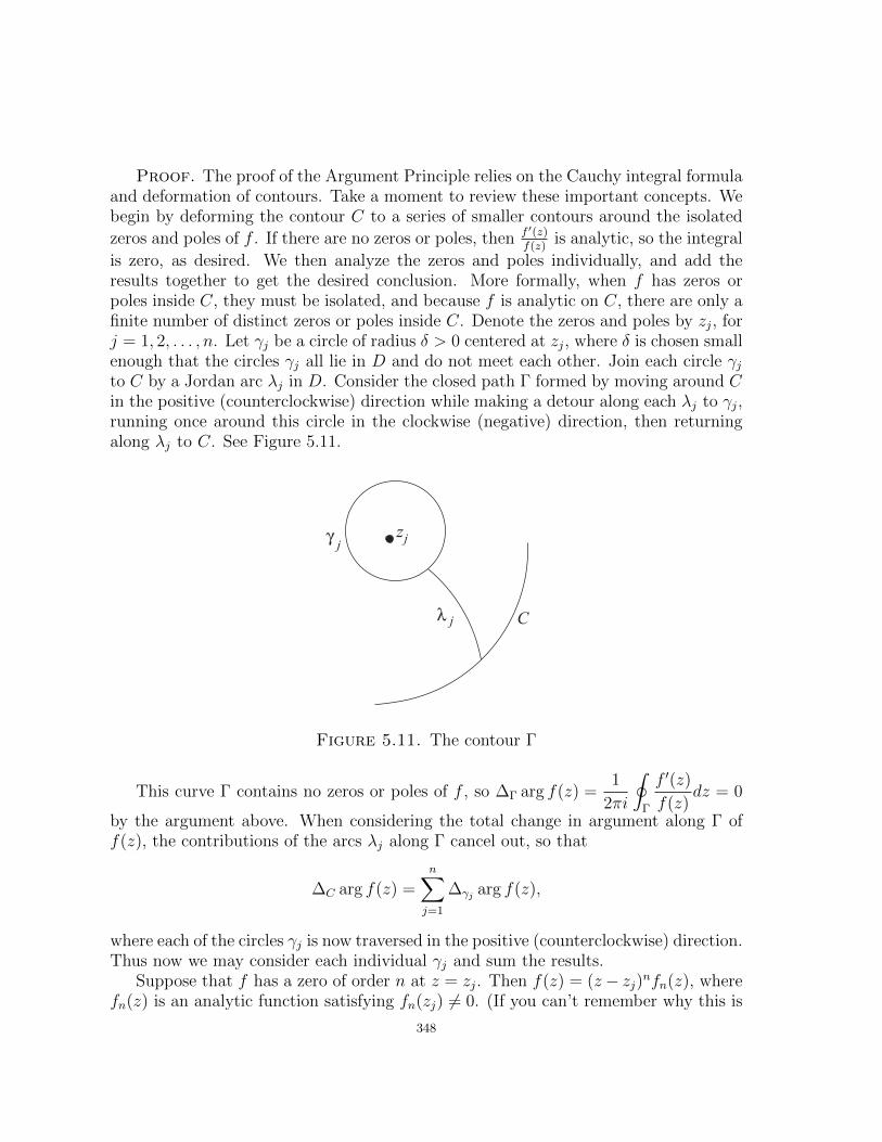
Proof. The proof of the Argument Principle relies on the Cauchy integral formulaand deformation of contours. Take a moment to review these important concepts. Webegin by deforming the contour C to a series of smaller contours around the isolated
zeros and poles of f . If there are no zeros or poles, then f ′(z)f(z)
is analytic, so the integral
is zero, as desired. We then analyze the zeros and poles individually, and add theresults together to get the desired conclusion. More formally, when f has zeros orpoles inside C, they must be isolated, and because f is analytic on C, there are only afinite number of distinct zeros or poles inside C. Denote the zeros and poles by zj, forj = 1, 2, . . . , n. Let γj be a circle of radius δ > 0 centered at zj, where δ is chosen smallenough that the circles γj all lie in D and do not meet each other. Join each circle γjto C by a Jordan arc λj in D. Consider the closed path Γ formed by moving around Cin the positive (counterclockwise) direction while making a detour along each λj to γj,running once around this circle in the clockwise (negative) direction, then returningalong λj to C. See Figure 5.11.
C
zjγ j
λ j
Figure 5.11. The contour Γ
This curve Γ contains no zeros or poles of f , so ∆Γ arg f(z) =1
2πi
∮Γ
f ′(z)
f(z)dz = 0
by the argument above. When considering the total change in argument along Γ off(z), the contributions of the arcs λj along Γ cancel out, so that
∆C arg f(z) =n∑j=1
∆γj arg f(z),
where each of the circles γj is now traversed in the positive (counterclockwise) direction.Thus now we may consider each individual γj and sum the results.
Suppose that f has a zero of order n at z = zj. Then f(z) = (z− zj)nfn(z), wherefn(z) is an analytic function satisfying fn(zj) 6= 0. (If you can’t remember why this is
348

true, look in any standard introductory complex analysis book.) Then
f ′(z) = n(z − zj)n−1fn(z) + (z − zj)nf ′n(z)
and
f ′(z)
f(z)=
n(z − zj)n−1fn(z) + (z − zj)nf ′n(z)
(z − zj)nfn(z)
=n
z − zj+f ′n(z)
fn(z).
Now we note that when we integrate the above expression along γj, we get n(2πi) + 0,
because f ′n(z)fn(z)
is analytic inside the contour.
Now suppose that f has a pole of order m at z = zk. This means that f can berewritten as f(z) = (z−zk)−mfm(z), where fm is analytic an nonzero at z = zk. Then,as previously, we have
f ′(z)
f(z)=−m(z − zk)−m−1fm(z) + (z − zk)−mf ′m(z)
(z − zk)−mfm(z)
=−mz − zk
+f ′m(z)
fm(z).
Once again, when we integrate the above expression along γk, we get −m(2πi) + 0.Summing over j = 1, 2, . . . n gives us the integral over Γ and the desired result.
5.4.2.2. Argument Principle for Harmonic Functions. There are many versions ofthe argument principle for harmonic functions. We only need the simple proof pre-sented in this section, developed by Duren, Hengartner, and Laugesen ([6]).
Theorem 5.47 (Argument Principle for Harmonic Functions). Let D be a Jordandomain with boundary C. Suppose f be a sense-preserving harmonic function on D,continuous in D and f(z) 6= 0 on C. Then ∆C arg f(z) = 2πN , where N is the totalnumber of zeros of f(z) in D, counted according to multiplicity.
Proof. First, we suppose that f has no zeros in D. This means that N = 0 andthe origin is not an element of f(D ∪ C). A fact from topology says that in this case,∆C arg f(z) = 0, and the theorem is proved. We will prove this fact. Let φ be ahomeomorphism of the closed unit square S onto D ∪ C with the restriction of φ tothe boundary, φ : ∂S → C, also a homeomorphism. See Figure 5.12.
The composition F = f φ is a continuous mapping of S onto the plane withno zeros, and we want to prove that ∆∂S argF (z) = 0. Begin by subdividing S intofinitely many small squares Sj so that on each Sj, the argument of F varies by atmost π/2. Then ∆∂Sj argF (z) = 0 (since F (Sj) cannot enclose the origin). Now whenwe consider ∆∂S argF (z), it is the sum
∑j ∆∂Sj argF (z) because the contributions to
349

S
F
fφ D C
Figure 5.12. The composition of f and φ.
the sum from the boundaries of each Sj cancel out, except where the boundary of Sjagrees with the boundary of S. Thus ∆∂S argF (z) = 0, as desired.
Now consider the case where f does have zeros in D. Because the zeros are isolated(as proven in Exercise 5.43), and because f is not zero on C, there are only a finitenumber of distinct zeros in D. We proceed in a manner similar to the proof of theanalytic argument principle, and, denote the zeros by zj, for j = 1, 2, . . . , n. Let γj bea circle of radius δ > 0 centered at zj, where δ is chosen so small that the circles γj alllie in D and do not meet each other. Join each circle γj to C by a Jordan arc λj in D.Consider the closed path Γ formed by moving around C in the positive direction whilemaking a detour along each λj to γj, running once around this circle in the clockwise(negative) direction, then returning along λj to C. (See Figure 5.11 on page 348.)This curve Γ contains no zeros of f , so ∆Γ argF (z) = 0 by the first case in this proof.When considering the total change in argument along Γ of f(z), the contributions ofthe arcs λj along Γ cancel out, so that
∆C arg f(z) =n∑j=1
∆γj arg f(z),
where each of the circles γj is now traversed in the positive (counterclockwise) direction.Thus now we may consider each individual γj and sum the results.
Now suppose that f has a zero of order n at a point z0. Then, as observed inExercise 5.43 on page 345, f can be locally written as
f(z) = an(z − z0)n(1 + ψ(z))
where an 6= 0 and |ψ(z)| < 1 on a sufficiently small circle γ defined by |z − z0| = δ.This shows that
(76) ∆γ arg f(z) = n∆γ arg(z − z0) + ∆γ arg(1 + ψ(z)) = 2πn.
350

Therefore, if f has zeros of order nj at the points zj, the conclusion is that
∆C arg f(z) =n∑j=1
∆γj arg f(z) = 2πn∑j=1
nj = 2πN,
and the theorem is proved.
Exercise 5.48. Justify why ∆γ arg(1 + ψ(z)) = 0 in Equation 76. Try it out!
For the next section, we shift our focus back to the polygonal maps defined inSection 5.3. We will be using the Argument Principle for Harmonic Functions in theproof of the Rado-Kneser-Choquet Theorem.
5.5. Rado-Kneser-Choquet Theorem
As you examine the image of the unit disk using the examples in Section 5.3,you may notice that some of the functions seem to be one-to-one on the interior ofthe domain, while others do not seem to be univalent. Look again at the examples,and compare functions which map to convex domains versus functions that map tonon-convex domains.
Exploration 5.49. Make a conjecture about when functions are one-to-one, usingthe exercises from Section 5.3 as a springboard. Do this before reading the Rado-Kneser-Choquet Theorem! Try it out!
In general, we completely understand the behavior of harmonic extensions (as de-fined in Definition 5.37) that map to convex regions:
Theorem 5.50 (Rado-Kneser-Choquet Theorem). Let Ω be a subset of C that
is a bounded convex domain whose boundary is a Jordan curve Γ. Let f map ∂Dcontinuously onto Γ and suppose that f(eit) runs once around Γ monotonically as eit
runs around ∂D. Then the harmonic extension given in the Poisson integral formulais univalent in D and defines a harmonic mapping of D onto Ω.
For the proof of this important theorem, we use the following lemma.
Lemma 5.51. Let ψ be a real-valued function harmonic in D and continuous in D.Suppose ψ has the property that, after a rotation of coordinates, ψ(eit)− ψ(e−it) ≥ 0on the interval [0, π], with strict inequality ψ(eit) − ψ(e−it) > 0 on some subinterval[a, b] with 0 ≤ a < b ≤ π. Then ψ has no critical points in D.
The condition on ψ seems a bit mysterious at first, and so we should discuss it. Onekind of function for which this property holds is a ψ that is at most bivalent on ∂D.What does “at most bivalent” mean? We know that univalent means that a function isone-to-one. Bivalent means that a function is two-to-one, or that there may be z1 6= z2
such that f(z1) = f(z2), but that if f(z1) = f(z2) = f(z3), then at least 2 of z1, z2, z3
351
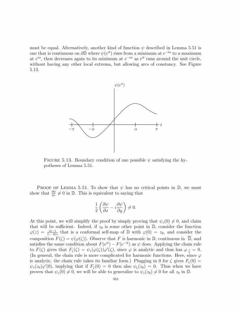
must be equal. Alternatively, another kind of function ψ described in Lemma 5.51 isone that is continuous on ∂D where ψ(eit) rises from a minimum at e−iα to a maximumat eiα, then decreases again to its minimum at e−iα as eit runs around the unit circle,without having any other local extrema, but allowing arcs of constancy. See Figure5.13. 1
ψ(eit)
−π −α α πt
Figure 5.13. Boundary condition of one possible ψ satisfying the hy-potheses of Lemma 5.51.
Proof of Lemma 5.51. To show that ψ has no critical points in D, we mustshow that ∂ψ
∂z6= 0 in D. This is equivalent to saying that
1
2
(∂ψ
∂x− i∂ψ
∂y
)6= 0.
At this point, we will simplify the proof by simply proving that ψz(0) 6= 0, and claimthat will be sufficient. Indeed, if z0 is some other point in D, consider the functionϕ(z) = z0−z
1− z0zthat is a conformal self-map of D with ϕ(0) = z0, and consider the
composition F (ζ) = ψ(ϕ(ζ)). Observe that F is harmonic in D, continuous in D, andsatisfies the same condition about F (eit)−F (e−it) as ψ does. Applying the chain ruleto F (ζ) gives that Fζ(ζ) = ψz(ϕ(ζ))ϕ′(ζ), since ϕ is analytic and thus has ϕ ζ = 0.(In general, the chain rule is more complicated for harmonic functions. Here, since ϕis analytic, the chain rule takes its familiar form.) Plugging in 0 for ζ gives Fζ(0) =ψz(z0)ϕ′(0), implying that if Fζ(0) = 0 then also ψζ(z0) = 0. Thus when we haveproven that ψz(0) 6= 0, we will be able to generalize to ψz(z0) 6= 0 for all z0 in D.
352

Now we use the Poisson integral formula to prove that ψz(0) 6= 0. Substituting in
ψ (or ψ(eit) = limr→1 ψ(reit) on ∂D) gives
ψ(z) =1
2π
∫ 2π
0
1− |z|2|eit − z|2 ψ(eit)dt =
1
2π
∫ 2π
0
1− z z(eit − z)(e−it − z)
ψ(eit)dt.
When we differentiate both sides with respect to z, the integral depends only on t, sowe are just left differentiating the integrand. Doing this, we find
∂
∂z
(ψ(eit)
1− z z(eit − z)(e−it − z)
)=
ψ(eit)
e−it − z
∂
∂z
(1− z zeit − z
)=
(ψ(eit)
e−it − z
)·(eit(e−it − z)
(eit − z)2
)= ψ(eit)
(eit
(eit − z)2
),
leading to the conclusion that
ψz(0) =1
2π
∫ 2π
0
ψ(eit)e−itdt.
From the hypotheses of the lemma, we know that there is some t ∈ (0, π) such thatψ(eit)− ψ(e−it) > 0. Thus
Imψz(0) = Im
(1
2π
∫ 2π
0
ψ(eit)e−itdt
)= − 1
2π
∫ 2π
0
ψ(eit) sin(t)dt
= − 1
2π
(∫ π
0
ψ(eit) sin(t)dt+
∫ 0
−πψ(eit) sin(t)dt
)since ψ is periodic
= − 1
2π
(∫ π
0
ψ(eit) sin(t)dt−∫ π
0
ψ(e−it) sin(t)dt
)= − 1
2π
∫ π
0
(ψ(eit)− ψ(e−it)) sin(t)dt < 0.
The last inequality relies on the fact that sin(t) is non-negative on the interval [0, π].We have now shown that Imψz(0) 6= 0, thus proving the lemma.
Proof of Theorem 5.50. Without loss of generality, assume that f(eit) runsaround Γ in the counterclockwise direction as t increases. (Otherwise, take conjugates.)We will show that if the function f is not locally univalent in D, then Lemma 5.51 willgive a contradiction.
353
Suppose that f = u+ iv is not locally univalent, or that the Jacobian of f vanishes
at some point z0 in D. This means that the matrix
(ux vxuy vy
)has a determinant of 0
at z0. From linear algebra, we know that this means that the system of equations
aux + bvx = 0
auy + bvy = 0
has a nonzero solution (a, b). Thus the real-valued harmonic function ψ = au+ bv hasa critical point at z0 (since (a, b) 6= (0, 0)). However, the hypothesis of Theorem 5.50implies that ψ satisfies the hypothesis of Lemma 5.51. Thus we have a contradiction,so f must be locally univalent.
Now that we see that f is locally univalent, we apply the argument principle toshow that f is univalent in D. Since f is sense-preserving on ∂D and locally univalent,f is sense-preserving throughout D. Now, if f is not univalent, there are two pointsz1 and z2 in D such that f(z1) = f(z2). However, that would imply that the functionf(z) − f(z1) has two zeros in D, so that the winding number of f(z) − f(z1) aboutthe origin is 2, which contradicts the hypotheses about the boundary correspondence.This completes the proof.
Exercise 5.52. Give a detailed proof of the statement, “However, the hypothesisof Theorem 5.50 implies that ψ satisfies the hypothesis of Lemma 5.51.” Try it out!
Notice that the description of f in Theorem 5.50 does not require that it be one-to-one on ∂D, but permits arcs of constancy. Furthermore, the Rado-Kneser-ChoquetTheorem is actually true in the case where f has jump discontinuities, as long asthe image of ∂D is not contained in a straight line. This requires some additionaljustification, so we state it separately as a corollary.
Corollary 5.53. Let f(z) be defined as in Definition 5.37 on 343. Suppose thevertices v1, v2, . . . vn, when traversed in order, define a convex polygon, with the interiorof the polygon denoted by Ω. Then the function f(z) is univalent in D and defines aharmonic mapping from D onto Ω.
Here is some intuition behind the proof of Corollary 5.53. Consider a sequence offunctions fm(eit) that are continuous and converge to the boundary correspondence
f(eit) of Definition 5.37. (One possible such sequence of functions can be described by
having fm(eit) = vk for t-values in the interval (tk−1 + tk−tk−1
2m, tk − tk−tk−1
2m) while for t-
values in the interval (tk− tk−tk−1
2m, tk+ tk+1−tk
2m), fm(eit) maps the interval linearly to the
segment between vk and vk+1.) Each of these functions fm(eit) satisfies the conditionsof the Rado-Kneser-Choquet Theorem, so extends to a univalent harmonic function,fm(z), in the unit disk. But the functions fm converge uniformly on compact subsetsof D, so the entire sequence converges uniformly to f in D. Therefore, f(z) inherits
354
the univalence from the sequence. The fact that the limit function is still univalent isnot immediately apparent–full details may be found in [8].
Interestingly enough, this theorem does not guarantee anything about univalenceif the domain Ω is not convex. In fact, the expectation is that univalence will not beachieved. For example, look at Exercise 5.34 on page 342.
Exploration 5.54. Extend the explorations begun in Exploration 5.35 on page343. Now, instead of modifying the boundary correspondence, start with the corre-spondence in Exercise 5.36. Then, move the vertex that is at i/2, moving it closer toi. A very nice picture comes from having the vertex set be 1, i,−1, 9i
10. In this last
we see the lack of univalence very clearly. Try it out!
5.5.1. Boundary behavior. In this section, we explore what seems to be truewith some of the above examples: There appears to be some very interesting boundarybehavior of our harmonic extensions of step functions. Examine this behavior in thefollowing exploration.
Exploration 5.55. Using ComplexTool or PolyTool, graph the function from Dto a triangle in Example 5.31. Now investigate the behavior of the boundary usingthe sketching tool of the applet. In particular, approach the break point between arcs(such as z = 1) along different paths. First approach radially, then approach along aline that is not a radius of the circle. Observe how these different paths that approach1 cause the image of the path to approach different points along the line segment thatmakes up a portion of the boundary of the range. (As you get very close to an arcendpoint, the image of the sketch may jump to a vertex–here, examine where the imageis immediately before that jump.) Technology hint: in PolyTool and ComplexTool, youcan hit the Graph button to clear all previous sketching but keep the polygonal map.Repeat this exercise with some of the other examples of polygonal functions. Try toanswer some of the following questions:
(1) Given a point ζ on the boundary of the polygon, is it possible to find a pathγ approaching ∂D such that γ(z) approaches ζ?
(2) As you approach an arc endpoint in ∂D radially, what point on the boundaryof the polygon do you approach?
Try it out!
As you performed the exploration above, you probably discovered some of theknown properties of the boundary behavior of harmonic extensions of step functions.These results were originally proven by Hengartner and Schober [8], who proved amore general form of the theorem below. We now restate their theorem as it appliesto the step functions of Definition 5.37. In the theorem below, the cluster set of f at apoint eitk is the set of all possible limits of sequences zn, where zn are inside Γ, andlimn→∞(zn) = eitk .
355

Theorem 5.56. Let f be the harmonic extension of a step function f(eitk) inDefinition 5.37. Denote by Γ the polygon defined by the vertices vk. By definition,the radial limits limr→1 f(reit) lie on Γ for all t except those in the set tk. Then theunrestricted limit
f(eit) = limz→eit
f(z)
exists at every point eit ∈ ∂D\eit1 , eit2 , ..., eitn and lies on Γ. Furthermore,
(1) the one-sided limits as t→ tk are
limt→t−k
f(eit) = vk and limt→t+k
f(eit) = vk+1; and
(2) the cluster set of f at each point eitk ∈ eit1 , eit2 , ..., eitn is the linear segmentjoining vk to vk+1.
Proof. Part (1) of the theorem follows directly from the definition of the functionf and from properties of the Poisson integral formula. That is, since the boundarycorrespondence is defined in Definition 5.37, the limits follow. Now we need to showpart (2). Now let us consider eitk . If z approaches eitk along the circular arc
(77) arg
(eitk + z
eitk − z
)=λπ
2, −1 < λ < 1,
then f(z) converges to the value
1
2(1− λ)vk +
1
2(1 + λ)vk+1.
Therefore the cluster set of f at tk is the line segment joining vk and vk+1, and part(2) is proven.
Exercise 5.57. Use basic ideas from analytic geometry to observe that equation77 is a circular arc. (Hint: First consider the cases where z is either on the circle or isthe center of the circle for some intuition.) Try it out!
Exercise 5.58. It is important to note that Theorem 5.56 holds for even non-univalent mappings. Go back to some of the previous examples and identify the linesegment that connnects the vertices. In particular, regraph the example from Exercise5.34. Using the Sketch utility in either ComplexTool or Polytool, check that the limitas you approach one of the tk does appear to be that line segment. Try it out!
5.6. Star Mappings
From the Rado-Kneser-Choquet Theorem, we see that harmonic functions map-ping the unit disk D to convex polygons are well-understood. That is, if we define aharmonic function mapping from the unit disk to a convex polygon as in Definition5.37, the function is univalent in D. Theorem 5.56 describes the boundary behavior
356
fully, showing that the limit of the function as we approach one of the break pointsbetween vertex pre-images, tk, gives the line segment joining the vertices.
However, non-convex polygons are not nearly as well-understood. We first examinenon-convex polygons in their simplest mathematical form: the ones of regular stars.
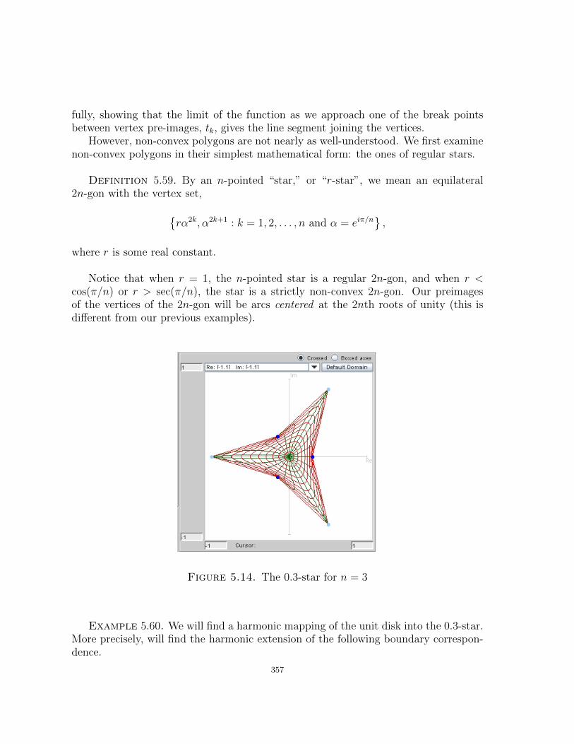
Definition 5.59. By an n-pointed “star,” or “r-star”, we mean an equilateral2n-gon with the vertex set,
rα2k, α2k+1 : k = 1, 2, . . . , n and α = eiπ/n,
where r is some real constant.
Notice that when r = 1, the n-pointed star is a regular 2n-gon, and when r <cos(π/n) or r > sec(π/n), the star is a strictly non-convex 2n-gon. Our preimagesof the vertices of the 2n-gon will be arcs centered at the 2nth roots of unity (this isdifferent from our previous examples).
Figure 5.14. The 0.3-star for n = 3
Example 5.60. We will find a harmonic mapping of the unit disk into the 0.3-star.More precisely, will find the harmonic extension of the following boundary correspon-dence.
357
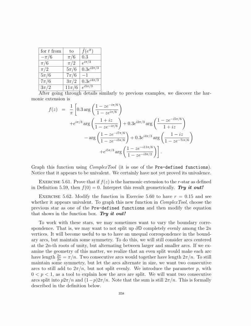
for t from to f(eit)−π/6 π/6 0.3π/6 π/2 eiπ/3
π/2 5π/6 0.3ei2π/3
5π/6 7π/6 −17π/6 3π/2 0.3ei4π/3
3π/2 11π/6 ei5π/3
After going through details similarly to previous examples, we discover the har-monic extension is
f(z) =1
π
[0.3 arg
(1− ze−iπ/61− zeiπ/6
)+eiπ/3 arg
(1 + iz
1− ze−iπ/6)
+ 0.3ei2π/3 arg
(1− ze−i5π/6
1 + iz
)− arg
(1− ze−i7π/61− ze−i5π/6
)+ 0.3ei4π/3 arg
(1− iz
1− ze−7iπ/6
)+ei5π/3 arg
(1− ze−i11π/6
1− ze−i3π/2)]
.
Graph this function using ComplexTool (it is one of the Pre-defined functions).Notice that it appears to be univalent. We certainly have not yet proved its univalence.
Exercise 5.61. Prove that if f(z) is the harmonic extension to the r-star as definedin Definition 5.59, then f(0) = 0. Interpret this result geometrically. Try it out!
Exercise 5.62. Modify the function in Exercise 5.60 to have r = 0.15 and seewhether it appears univalent. To graph this new function in ComplexTool, choose theprevious star as one of the Pre-defined functions and then modify the equationthat shows in the function box. Try it out!
To work with these stars, we may sometimes want to vary the boundary corre-spondence. That is, we may want to not split up ∂D completely evenly among the 2nvertices. It will become useful to us to have an unequal correspondence in the bound-ary arcs, but maintain some symmetry. To do this, we will still consider arcs centeredat the 2n-th roots of unity, but alternating between larger and smaller arcs. If we ex-amine the geometry of this matter, we realize that an even split would make each archave length 2π
2n= π/n. Two consecutive arcs would together have length 2π/n. To still
maintain some symmetry, but let the arcs alternate in size, we want two consecutivearcs to still add to 2π/n, but not split evenly. We introduce the parameter p, with0 < p < 1, as a tool to explain how the arcs are split. We will want two consecutivearcs split into p2π/n and (1−p)2π/n. Note that the sum is still 2π/n. This is formallydescribed in the definition below.
358

Definition 5.63. Let n ≥ 2 be a fixed integer, r be a positive real number, andα = eiπ/n. Define a boundary correspondence for all but a finite number of points on∂D by mapping arcs with endpoints αe−ipπ/n, αeipπ/n, 0 ≤ k ≤ n− 1 as follows:
(78) f(eit) =
rα2k , eit ∈ (α2ke−ipπ/n, α2keipπ/n)α2k+1 , eit ∈ (α2k+1e−i(1−p)π/n, α2k+1ei(1−p)π/n)
.
Let f be the Poisson extension of f .
eiπ/n
r2pπ/n
2(1 - p)πn
Figure 5.15. The first two arcs and their images according to Defini-tion 5.63. The dots on the left-hand-side indicate points of discontinuityof the boundary correspondence.
Note that the arc (α2ke−ipπ/n, α2keipπ/n) centered at α2k is mapped to the vertexrα2k and the arc (α2k+1e−i(1−p)π/n, α2k+1ei(1−p)π/n) centered at α2k+1 is mapped to thevertex α2k+1.
Exercise 5.64. Show that the interval in the second half of Equation 78,
(α2k+1e−i(1−p)π/n, α2k+1ei(1−p)π/n),
can be written more compactly as (α2keipπ/n, α2k+2e−ipπ/n). Try it out!
At this point, you should start using with the StarTool applet. The default for thisapplet is the 3-pointed star discussed in Example 5.60. Note that the arcs and theirtarget vertices are color-coded (with a light blue arc mapping to a light blue vertex,for example). The default p-value is 0.5, which corresponds to evenly spaced arcs.You can use the slider bars (the plus/minus buttons for n) or type in the text boxesto change the values for n, p, and r. The maximum n-value allowed by the applet isn = 18, which is sufficient for the explorations below. As with ComplexTool, there isthe option to Sketch on the graph to get a better feel for the mapping properties ofthese stars. There is also an option to Show roots of ω(z). The roots of ω(z) willbe helpful in future discussion, but are not essential for the starting explorations. Ingeneral, try to first get a good feel for what happens for “small” values of n, such as4, 5, 6, or 7.
359
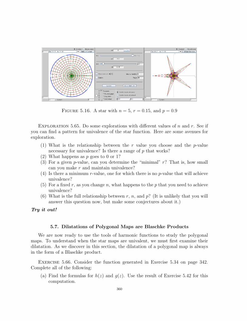
Figure 5.16. A star with n = 5, r = 0.15, and p = 0.9
Exploration 5.65. Do some explorations with different values of n and r. See ifyou can find a pattern for univalence of the star function. Here are some avenues forexploration.
(1) What is the relationship between the r value you choose and the p-valuenecessary for univalence? Is there a range of p that works?
(2) What happens as p goes to 0 or 1?(3) For a given p-value, can you determine the “minimal” r? That is, how small
can you make r and maintain univalence?(4) Is there a minimum r-value, one for which there is no p-value that will achieve
univalence?(5) For a fixed r, as you change n, what happens to the p that you need to achieve
univalence?(6) What is the full relationship between r, n, and p? (It is unlikely that you will
answer this question now, but make some conjectures about it.)
Try it out!
5.7. Dilatations of Polygonal Maps are Blaschke Products
We are now ready to use the tools of harmonic functions to study the polygonalmaps. To understand when the star maps are univalent, we must first examine theirdilatation. As we discover in this section, the dilatation of a polygonal map is alwaysin the form of a Blaschke product.
Exercise 5.66. Consider the function generated in Exercise 5.34 on page 342.Complete all of the following:
(a) Find the formulas for h(z) and g(z). Use the result of Exercise 5.42 for thiscomputation.
360

(b) Find the derivatives h′(z) and g′(z), verifying that the derivatives simplify to
h′(z) =1
(2πi)(1− z4)
((3
2− 3
2i)z2 − 3iz + (
5
2+
5
2i)
)and g′(z) =
1
(2πi)(1− z4)
((5
2− 5
2i)z2 + 3iz + (
3
2+
3
2i)
).
(c) Show that the zeros of g′(z) are z1 ≈ 0.9245 − 0.9245i and z2 ≈ −0.3245 +0.3245i, and that the zeros of h′(z) are 1/ z1 and 1/ z2. Thus we are able towrite the dilatation as
ω(z) = C
(z1 − z
1− z1z
)(z2 − z
1− z2z
),
where C is some constant.(d) What are |z1|, |z2|, and |C|? These will be helpful to recall as we look ahead
to Theorem 5.81 in Section 5.8.
Try it out!
Motivated by the results of Exercise 5.66, we now examine functions that are of aparticular form.
Exploration 5.67. We examine the properties of functions of the formBz0(z) =z0 − z
1− z0z.
• Using ComplexTool, graph the image of the unit disk under the functions
B0.5(z) = 0.5−z1−0.5z
, B0.5 exp(iπ/4)(z) = 0.5eiπ/4−z1−0.5e−iπ/4z
, and B0.5i(z) = 0.5i−z1+0.5iz
. What is
B(0)? What is the image of the unit disk under B(z)? Does B(z) appear tobe univalent?• Now graph the image of the unit disk under the function B2 exp(iπ/4)(z) =
2eiπ/4−z1−2e−iπ/4z
. What is B(0)? What is the image of the unit disk under B(z)?
Does B(z) appear to be univalent?• If we consider Bz0(z), can we determine Bz0(0) in general? What effect does
arg(z0) have on the location of Bz0(0)? What effect does |z0| have on theimage of the unit disk?• Now let’s multiply the functions Bz0(z). First graph the image of the unit
disk under f1(z) = (B0.5(z))2 =(
0.5−z1−0.5z
)2. What is f(0)? What is the image
of the unit disk under f(z)? Does f(z) appear to be univalent? How does thiscompare to the function f(z) = z2?• Now graph the image of the unit disk under f2(z) = B0.5(z)B0.5i(z), f3(z) =B0.5(z)B0.2i(z), and f4(z) = B0.5 exp(iπ/4)(z)B0.2i(z). What are f2(0), f3(0),and f4(0)? How do f2(0), f3(0), and f4(0) relate to the values of z0 in thefunctions Bz0(z)?
Try it out!
361
Definition 5.68. A Blaschke factor is Bz0(z) = z0−z1− z0z
, and a finite Blaschkeproduct or order n is a product of n Blaschke factors, possibly multiplied by a constantζ such that |ζ| = 1:
ζn∏k=1
zk − z1− zkz
.
Note that the multiplication by ζ is simply a rotation.
Remark 5.69. It is important to note that the Blashke product definition givenabove is a bit non-standard. The standard definition of Blaschke product, as given inChapters 4 and 6, assumes that |zk| < 1. Here we do not place that restriction on zkfor the purpose of simplifying our computations.
In this section, we use the result of Exercise 5.39 on page 344 to see that thedilatation of the harmonic polygonal functions to an n-gon is a Blaschke product oforder at most n − 2. This result was proven by T. Sheil-Small in [17], and is alsodiscussed in [5].
We use the notation fk(z) to denote the contribution to the function f(z) thatarises from applying the Poisson integral formula to the boundary correspondence fortk−1 < t < tk. We then have f(z) =
∑nk=1 fk(z). On the interval tk−1 < t < tk, we
observe that
fk(z) =vk2π
(tk − tk−1) +vkπ
arg
(1− ze−itk
1− ze−itk−1
)by Definition 5.37. We now consider the canonical decomposition of fk(z) = hk(z)+ gk(z).By Exercise 5.42, we have
hk(z) =vk2π
(tk − tk−1) +vk2πi
log
(1− ze−itk
1− ze−itk−1
)=
vk2π
(tk − tk−1) +vk2πi
(log(1− ze−itk)− log(1− ze−itk−1)
)and
gk(z) =vk
2πilog
(1− ze−itk
1− ze−itk−1
)=
vk2πi
(log(1− ze−itk)− log(1− ze−itk−1)
).
The computations that follow will give some rigor to our intuition: since h and gare sums of logarithms, their derivatives are sums of terms that have 1− ze−itk in thedenominators. We will combine these factors, and hope that we can see each derivativeas a Blaschke product. Now, when we look at h(z) =
∑nk=1 hk(z) and take derivatives,
362

we see that:
h′(z) =n∑k=1
vk2πi
( −e−itk1− ze−itk −
−e−itk−1
1− ze−itk−1
)(79)
=n∑k=1
vk2πi
(1
z − eitk −1
z − eitk−1
).(80)
The function g′(z) is identical except for having vk instead of vk:
g′(z) =n∑k=1
vk2πi
( −e−itk1− ze−itk −
−e−itk−1
1− ze−itk−1
)(81)
=n∑k=1
vk2πi
(1
z − eitk −1
z − eitk−1
).(82)
Combining like factors gives us a more compact form, with
(83) h′(z) =1
2πi
n∑k=1
vk − vk+1
z − eitk and g′(z) =1
2πi
n∑k=1
vk − vk+1
z − eitk .
It will be useful for the upcoming discussion to note that∑n
k=1(vk − vk+1) = 0,since vn+1 = v1.
Exercise 5.70. Prove that∑n
k=1(vk − vk+1) = 0, since vn+1 = v1. Interpret thisresult geometrically.
Try it out!
We rely heavily upon the observation that
(84) h′(1/ z) = z2g′(z) or g′(1/ z) = z2h′(z).
363

Equation 84 arises from the following computation:
h′(1/ z)− z2g′(z) =−1
2πi
n∑k=1
vk − vk+1
1/z − e−itk −z2
2πi
n∑k=1
vk − vk+1
z − eitk
=−z2πi
n∑k=1
eitk( vk − vk+1)
eitk − z − z2
2πi
n∑k=1
vk − vk+1
z − eitk
=z
2πi
n∑k=1
eitk( vk − vk+1)
z − eitk − z2
2πi
n∑k=1
vk − vk+1
z − eitk
=1
2πi
n∑k=1
( vk − vk+1)(zeitk − z2)
z − eitk
=1
2πi
n∑k=1
( vk − vk+1)(z)(eitk − z)
z − eitk
=−1
2πi
n∑k=1
( vk − vk+1)(z)
= 0.
Exercise 5.71. We have just proven the first half of Equation 84. Using thatresult, prove the second part of Equation 84 with minimal calculation. Try it out!
Exercise 5.72. Interpret this result geometrically. That is, note that if we havea value z0 ∈ D such that g′(z0) = 0, then what do we know about the zeros of h′?How are the locations of the zeros of h′ related to the locations of the zeros of g′?Completion of this exercise will give some intuition about the proof that is to come.Try it out!
Exercise 5.73. Show that h′(z) and g′(z) of Exercise 5.66 satisfy Equation 84.Relate this to the previous two exercises–do the conclusions of those exercises alsohold true for this example? Try it out!
For simplicity of notation, let us consider the functions h′(z) and g′(z). We canalready tell that if we got a common denominator for h′(z) or g′(z), that the denomi-
nator would ben∏k=1
(z − eitk), and we would guess that the ratio of the two would give
us a product of rational functions. At this point, that is all we can tell–it is not obviousthat this product should be a Blaschke product, although we may expect it to be fromthe explorations we did in Exercise 5.66. The remainder of this section will be devotedto determining that this is, indeed, a Blaschke product, as well as finding the order ofthat product.
364
Exploration 5.74. Based on the results of Exercise 5.66, and upon other examplesin this chapter, make a conjecture about the number of Blaschke factors that shouldbe in the dilatation of a harmonic function from D to an n-gon. Try it out!
Obtaining a common denominator for both h′ and g′, we can look at them as
h′(z) =P (z)
S(z)and g′(z) =
Q(z)
S(z),
where S(z) =n∏k=1
(z − eitk) . Now we need to consider what P and Q look like. Consider
that by brute force, each term of the P (z) looks like (vk − vk+1)n∏
j=1;j 6=k
(z − eitj), or,
put more simply, a polynomial of degree at most n− 1. Let us consider the zn−1 term
of P (z). It is simply vk − vk+1 for each piece of the sum, so it must ben∑k=1
(vk − vk+1),
which we already observed to be 0. Thus we have shown that P (z) has degree at mostn− 2. The same argument works for Q(z), since it has the same structure as P (z) butwith conjugates over the vk.
We now turn our attention to the denominator, which is S(z) =n∏k=1
(z − eitk).
Exercise 5.75. Show that the following equation holds:
S(1/ z) =
(1
z
)n(−1)n S(z)
n∏k=1
eitk .
Try it out!
Put another way, we could write
(85) S(1/ z) =
(1
z
)n(−1)nS(z)
n∏k=1
e−itk .
Exercise 5.76. Show that Equation 85 holds for the denominator of the derivativesin Exercise 5.66, 2πi(1− z4). Try it out!
Now we can combine Equations 84 and 85 to get a relationship between P (z) and
Q(z). Directly substituting into h′(1/ z) = z2g′(z), we see that
365
h′(1/ z) = z2g′(z)
P (1/ z)
S(1/ z)= z2Q(z)
S(z)
P (1/ z)(1z
)n(−1)nS(z)
∏nk=1 e
−itk= z2Q(z)
S(z).
This leads to the relationship
(86) zn−2 P (1/ z) = (−1)nQ(z)n∏k=1
e−itk .
Exercise 5.77. Using the result above, show that
(87) zn−2 Q(1/ z) = (−1)nP (z)n∏k=1
e−itk .
Try it out!
Since the function f is orientation-preserving, we know that h′(z) 6= 0 in D. Thisimplies that P (z) 6= 0 in D. In particular, P (0) 6= 0. Substituting 0 into equation 87,we find that the left hand side must not be zero, which forces the degree of Q to beat least n − 2. However, we had previously determined that the degree of Q must beat most n− 2. Thus the degree of Q is n− 2. Similarly, the degree of P is also n− 2.Since the degree of Q is n− 2, let us write
Q(z) = zmn−m−2∏k=1
(z − zk)
to show that Q may have m zeros at the origin and n −m − 2 zeros elsewhere (notethat the zk need not be distinct). Now using Equation 87, we can write
zn−2
(1
z
)m n−m−2∏k=1
(1
z− zk
)= (−1)nP (z)
n∏k=1
e−itk .
The left hand side of the above equation may be rewritten as
zn−m−2 1
zn−m−2
n−m−2∏k=1
(1− z zk) .
At this point we can see that since the zeros of Q are zk, the zeros of P are the zeros ofn−m−2∏k=1
(1− z zk), which are precisely 1/ zk. Now we are able to see what the Blaschke
product is.
366
Exercise 5.78. Find the relationship between the number of zeros of Q and thenumber of zeros of P . In particular, if Q has degree n− 2 with m zeros at the originand n−m− 2 zeros away from the origin, then how many of the zeros of P are at theorigin? How many of the zeros of P are away from the origin? Try it out!
We now summarize the results of our work in this section (as originally proved byT. Sheil-Small, [17] Theorem 1; see also [5]).
Theorem 5.79. Let f be the harmonic extension of the step function f(eit) asgiven in Definition 5.37. Then
g′(z) =Q(z)
S(z)and h′(z) =
P (z)
S(z),
where Q(z), P (z), and S(z) are defined as above, and P and Q are polynomials ofdegree at most n− 2. Furthermore, their ratio ω(z) satisfies |ω(z)| = 1 when |z| = 1,so takes the form of a Blaschke product of degree at most n− 2.
5.8. An Important Univalence Theorem
In this section, we examine a theorem of Sheil-Small that tells when the harmonicfunction in Definition 5.37 is univalent. In particular, the location of the zeros of the
analytic dilatation ω(z) = g′(z)h′(z)
are sufficient to tell when the harmonic function is
univalent.
Exploration 5.80. Open up the StarTool applet. Check the box in front of Showroots of ω(z). You will see extra dots appear in the right-hand pane (the range ofthe function), as well as a unit circle for reference. These dots denote the locationsof the zeros of the dilatation ω(z). Now experiment with the values of p and r to seeif there is a relationship between the roots of ω(z) and whether the resulting star isunivalent. Do this for various values of n to see if your result seems to hold. Doesyour conjecture agree with the examination of a function that maps D to a differentnon-convex polygon, as in Exercise 5.66? Try it out!
The theorem below was proven by Sheil-Small, and is Theorem 11.6.6 of [18].
Theorem 5.81. Let f be a harmonic function of the form in Definition 5.37. Herethe function f is the harmonic extension of a piecewise constant boundary functionwith values on the m vertices of a polygonal region Ω, so that, by Theorem 5.79, thedilatation of f is a Blaschke product with at most m− 2 factors. Then f is univalentin D if and only if all zeros of ω lie in D. In this case, f is a harmonic mapping of Donto Ω.
Proof. First, suppose that f is univalent in D. If a Blaschke factor is defined asϕz0(z) = z0−z
1− z0z, with the constant z0 not having modulus 1, then we notice that since
the dilatation ω is a product of a finite number of Blaschke factors, ω(z) 6= 0 on theunit circle. This is because the zero of the Blaschke factor is z0, and if |z0| = 1, we get
367
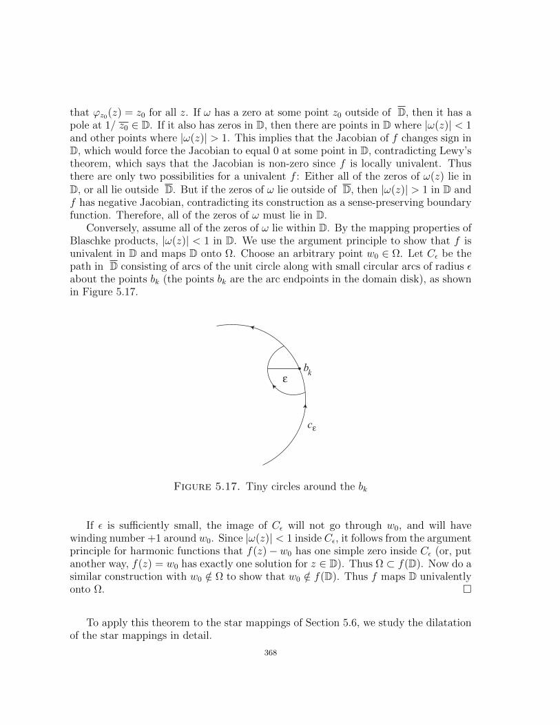
that ϕz0(z) = z0 for all z. If ω has a zero at some point z0 outside of D, then it has apole at 1/ z0 ∈ D. If it also has zeros in D, then there are points in D where |ω(z)| < 1and other points where |ω(z)| > 1. This implies that the Jacobian of f changes sign inD, which would force the Jacobian to equal 0 at some point in D, contradicting Lewy’stheorem, which says that the Jacobian is non-zero since f is locally univalent. Thusthere are only two possibilities for a univalent f : Either all of the zeros of ω(z) lie inD, or all lie outside D. But if the zeros of ω lie outside of D, then |ω(z)| > 1 in D andf has negative Jacobian, contradicting its construction as a sense-preserving boundaryfunction. Therefore, all of the zeros of ω must lie in D.
Conversely, assume all of the zeros of ω lie within D. By the mapping properties ofBlaschke products, |ω(z)| < 1 in D. We use the argument principle to show that f isunivalent in D and maps D onto Ω. Choose an arbitrary point w0 ∈ Ω. Let Cε be thepath in D consisting of arcs of the unit circle along with small circular arcs of radius εabout the points bk (the points bk are the arc endpoints in the domain disk), as shownin Figure 5.17.
bk
cε
ε
Figure 5.17. Tiny circles around the bk
If ε is sufficiently small, the image of Cε will not go through w0, and will havewinding number +1 around w0. Since |ω(z)| < 1 inside Cε, it follows from the argumentprinciple for harmonic functions that f(z)−w0 has one simple zero inside Cε (or, putanother way, f(z) = w0 has exactly one solution for z ∈ D). Thus Ω ⊂ f(D). Now do asimilar construction with w0 /∈ Ω to show that w0 /∈ f(D). Thus f maps D univalentlyonto Ω.
To apply this theorem to the star mappings of Section 5.6, we study the dilatationof the star mappings in detail.
368
5.9. The Dilatation for Star Mappings
In this section, we will use Definition 5.63 of Section 5.6 as the starting point. Wewill build upon the basic formula for the functions h′(z) and g′(z), and then will simplifythe dilatation ω(z) as a Blaschke product. By doing so, we completely determine whichstar functions are univalent.
Using Equations (79) and (81) of Section 5.7, along with Definition 5.63, we findthe following equations for h′(z) and g′(z) for the star functions:
h′(z) =rα0
2πi
(1
z − α0eipπ/n− 1
z − α0e−ipπ/n
)+α
2πi
(1
z − α2e−ipπ/n− 1
z − α0eipπ/n
)+rα2
2πi
(1
z − α2eipπ/n− 1
z − α2e−ipπ/n
)+ . . .
=r
2πi
n−1∑k=0
α2k
(1
z − α2keipπ/n− 1
z − α2ke−ipπ/n
)(88)
+1
2πi
n−1∑k=0
α2k+1
(1
z − α2k+2e−ipπ/n− 1
z − α2keipπ/n
)and
g′(z) =r
2πi
n−1∑k=0
α2k
(1
z − α2keipπ/n− 1
z − α2ke−ipπ/n
)(89)
+1
2πi
n−1∑k=0
α2k+1
(1
z − α2k+2e−ipπ/n− 1
z − α2keipπ/n
).
Our goal is to express ω(z) = g′(z)/h′(z) as the ratio of Blaschke products guaranteedby Sheil-Small’s work. To that end, we first establish a few general algebraic identitiesinvolving sums of the quantities of the type found in the expansions of h′(z) and g′(z)above.
It is a basic complex identity that if ζ is a primitive mth root of unity, then
(90)m∏k=1
(z − ζk) = zm − 1.
Exercise 5.82. Prove Equation (90). Interpret this result geometrically. Try itout!
369
Exercise 5.83. Again, let ζ be a primitive mth root of unity. Show that
(91)m−1∏k=0
(z − ζka) = zm − am.
Hint: Replace z with z/a in Equation (90). Try it out!
Now we work to answer the hard question: How do we add together all of the sumsin equations (88) and (89), given that their numerators are not simply the constant 1?As an intermediate step toward achieving this, we establish the following identity.
Lemma 5.84. If ζ is a primitive mth root of unity, then
(92)m−1∑k=0
ζk
z − ζka =mam−1
zm − am .
Exercise 5.85. Prove the lemma, using the following steps in the partial fractiondecomposition.
(1) Recall Equation (91) and note how it fits in with this formula.(2) Note that since we have n distinct linear factors in the denominator, we can
expect to find that
mam−1
zm − am =m−1∑k=0
akz − ζka.
(3) We will find an arbitrary ak0 . By setting z = ζk0a, establish that
ak0 =mam−1∏
k 6=k0(ζk0a− ζka)
=m∏
k 6=k0(ζk0 − ζk) .
(4) Show that∏k 6=k0
(ζk0 − ζk) = mζ−k0 . It will be helpful to remember that ζk0 is
an mth root of unity, so ζk0m = 1.(5) Conclude that ak0 = ζk0 .(6) Equation (92) should follow.
Try it out!
We now recall the result of Exercise 5.64 on page 359 that
α2k+2e−ipπ/n = α2k+1ei(1−p)π/n and α2keipπ/n = α2k+1e−i(1−p)π/n.
Combining with the earlier work, we have
370
1
2πi
n−1∑k=0
α2k+1
z − α2k+2e−ipπ/n=−1
2πi
(nei(1−p)(n−1)π/n
zn + ei(1−p)π
)and
− 1
2πi
n−1∑k=0
α2k+1
z − α2keipπ/n=
1
2πi
(ne−i(1−p)(n−1)π/n
zn + e−i(1−p)π
).
Exercise 5.86. Prove that
− 1
2πi
n−1∑k=0
α2k+1
z − α2keipπ/n=
1
2πi
(ne−i(1−p)(n−1)π/n
zn + e−i(1−p)π
).
Try it out!
Combining all of these together, we see that
h′(z) =n
2πi
(rei(
n−1n
)pπ
zn − eipπ +−re−i(n−1
n)pπ
zn − e−ipπ
+−ei(n−1
n)(1−p)π
zn + ei(1−p)π+e−i(
n−1n
)(1−p)π
zn + e−i(1−p)π
).(93)
We need to keep our goal in mind: We know from Theorem 5.79 that g′(z)h′(z)
can be
written as a Blaschke product. To do this, we will have to find a common denominatorand combine the four terms of h′(z) to see the quotient. As an initial step, we findthat we can write the common denominator more simply than it first appears.
Exercise 5.87. Prove that (zn− eipπ)(zn− e−ipπ) = (zn + ei(1−p)π)(zn + e−i(1−p)π).We will call this product Sn(z). Try it out!
Exercise 5.88. Using basic algebra (finding a common denominator, simplifying,and using properties of z + z), prove that
h′(z) =n
πSn(z)
(zn(r sin
((n− 1)pπ
n
)− sin
((n− 1)(1− p)π
n
))(94)
+r sin(pπn
)+ sin
((1− p)π
n
)).
Try it out!
Through methods similar to those of the simplification of h′(z), we can also provethat
g′(z) =nzn−2
πSn(z)
(zn(r sin
(pπn
)+ sin
((n− 1)(1− p)π
n
))(95)
+r sin
((n− 1)pπ
n
)− sin
((n− 1)(1− p)π
n
)).
371
With this simplified form of g′(z), we use
(96) c =sin (n−1)(1−p)π
n− r sin (n−1)pπ
n
r sin pπn
+ sin (1−p)πn
to write
(97) g′(z) =nzn−2
π
(r sin
(pπn
)+ sin
((1− p)π
n
))zn − cSn(z)
.
Now we are ready to pull together the result of Theorem 5.81 and the dilatationthat we just simplified. When the zeros of this dilatation are within the unit disk, thenthe harmonic function f = h+ g that defines the star is univalent. By a straightforwardcomputation, we find that the dilatation of f is
(98) ω(z) =zn−2(zn − c)
1− znc .
Exercise 5.89. Look again at Theorem 5.81 and verify that it does, indeed, holdfor the star function. Try it out!
Exploration 5.90. Notice that f is univalent when |c| < 1. Using that observa-tion, do the following:
• Use the StarTool applet to explore graphically what relationship there is be-tween n, p, and c.• For a fixed n, find the range of p-values that make |c| < 1.• For a fixed p, find the range of n-values that make |c| < 1.
Try it out!
Large Project 5.91. If you move just one vertex of the star, do the same resultshold for the relationship between n and p? (For example, take the vertex at r, andmove it to r + ε or r − ε. Is the star still univalent?)
Exercise 5.92. For a given n, consider the formula for c in Equation 96 to be afunction of p alone. Prove that any star configuration is possible; that is, prove thatfor any value of r, a value of p can be found to make |c| < 1. What ranges of p makesthis happen? Conversely, prove that for all values of r < cos(π/n) or r > sec(π/n),a p can be chosen to make the function NOT univalent. Why is this not true forcos(π/n) ≤ r ≤ sec(π/n)? For more information, see Theorem 4 in [7]. Try it out!
Small Project 5.93. Refer to Chapter 2. For what values of c is the dilatation aperfect square? Find and describe the associated minimal surfaces. Can these surfacesbe described as examples of other well-known surfaces? For more information on thisproject, see [12].
372
5.10. Open Questions
Large Project 5.94. Can we map to any polygon univalently? The star setuptakes full advantage of the symmetry. Once you lose that advantage, it is much harderto discover whether the zeros of the dilatation have modulus less than 1. This questionis known as the Mapping Problem, proposed by T. Sheil-Small in [17].
Small Project 5.95. Look at a function f that is not univalent. Now look atthe set S ⊂ D of points on which the function f is univalent. First, how do you findthat set? What is the shape of S? Is it starlike? Is it convex? Is it connected? Is itsimply connected? Can D\S be connected?
Small Project 5.96. In this chapter, we discussed one way of proving that aharmonic function is univalent by looking at zeros of the analytic dilatation ω(z). InChapter 4, there is another set of criteria for univalence, as demonstrated in Section 4.6.Connect these two avenues of investigation. For example, does one imply the other?How does the work with stars in this chapter generalize to the approach in Chapter 4?Are there results in this chapter that could not be found using the methods of Chapter4?
373

Bibliography
1. Lars Ahlfors, Complex analysis, third ed., McGraw-Hill, New York, 1979.2. W. N. Bailey, Generalized hypergeometric series, Cambridge Tracts in Mathematics and Mathe-
matical Physics, No. 32, Stechert-Hafner, Inc., New York, 1964. MR MR0185155 (32 #2625)3. Tobin A. Driscoll and Lloyd N. Trefethen, Schwarz-christoffel mapping, Cambridge University
Press, Cambridge, 2002.4. Kathy Driver and Peter Duren, Harmonic shears of regular polygons by hypergeometric functions,
J. Math. Anal. Appl. 239 (1999), no. 1, 72–84. MR 2000k:300085. Peter Duren, Harmonic mappings in the plane, Cambridge Tracts in Mathematics, vol. 156,
Cambridge University Press, Cambridge, 2004. MR 2 048 3846. Peter Duren, Walter Hengartner, and Richard S. Laugesen, The argument principle for harmonic
functions, Amer. Math. Monthly 103 (1996), no. 5, 411–415. MR 97f:300027. Peter Duren, Jane McDougall, and Lisbeth Schaubroeck, Harmonic mappings onto stars, J. Math.
Anal. Appl. 307 (2005), no. 1, 312–320. MR MR21389928. W. Hengartner and G. Schober, Harmonic mappings with given dilatation, J. London Math. Soc.
(2) 33 (1986), no. 3, 473–483. MR MR850963 (87j:30037)9. Elgin Johnston, A “counterexample” for the Schwarz-Christoffel transform, Amer. Math. Monthly
90 (1983), no. 10, 701–703. MR MR723944 (85f:30009)10. Serge Lang, Complex analysis, fourth ed., Graduate Texts in Mathematics, vol. 103, Springer-
Verlag, New York, 1999. MR MR1659317 (99i:30001)11. H. Lewy, On the non-vanishing of the jacobian in certain one-to-one mappings, Bull. Amer. Math.
Soc. 42 (1936), no. 1, 689–692.12. Jane McDougall and Lisbeth Schaubroeck, Minimal surfaces over stars, J. Math. Anal. Appl. 340
(2008), no. 1, 721–738. MR MR237619213. Zeev Nehari, Conformal mapping, Dover Publications Inc., New York, 1975, Reprinting of the
1952 edition. MR MR0377031 (51 #13206)14. Earl D. Rainville, Special functions, The Macmillan Co., New York, 1960. MR MR0107725 (21
#6447)15. E.B. Saff and A.D. Snider, Fundamentals of complex analysis for mathematics, science, and
engineering, 2nd ed., Prentice Hall, Upper Saddle River, NJ, 1993.16. Roland Schinzinger and Patricio A. A. Laura, Conformal mapping: Methods and applications,
Dover Publications Inc., New York, 2003, Reprinting of the 1991 edition.17. T. Sheil-Small, On the Fourier series of a step function, Michigan Math. J. 36 (1989), no. 3,
459–475. MR 91b:3000218. , Complex polynomials, Cambridge Studies in Advanced Mathematics, vol. 75, Cambridge
University Press, Cambridge, 2002. MR MR1962935 (2004b:30001)19. Richard A. Silverman, Complex analysis with applications, Dover Publications Inc., New York,
1984, Reprint of the 1974 original. MR MR781933 (86c:30004)20. Dennis G. Zill and Patrick D. Shanahan, A first course in complex analysis with applications,
Jones and Bartlett, Sudbury, MA, 2003.
374