Mapping of Applications to Platforms Peter Marwedel TU Dortmund, Informatik 12 Germany Graphics: ©...
32
Mapping of Applications to Platforms Peter Marwedel TU Dortmund, Informatik 12 Germany Graphics: © Alexandra Nolte, Gesine Marwedel, 2003 These slides use Microsoft clip arts. Microsoft copyright restrictions apply. 2011 年 06 年 22 年
-
Upload
santos-rushton -
Category
Documents
-
view
214 -
download
0
Transcript of Mapping of Applications to Platforms Peter Marwedel TU Dortmund, Informatik 12 Germany Graphics: ©...
Mapping of Applications to
Platforms
Peter MarwedelTU Dortmund, Informatik 12
Germany
Gra
phic
s: ©
Ale
xand
ra N
olte
, Ges
ine
Mar
wed
el, 2
003
These slides use Microsoft clip arts. Microsoft copyright restrictions apply. 2011 年 06 月 22 日

- 2 - p. marwedel, informatik 12, 2011
Structure of this course
2:Specification
3: ES-hardware
4: system software (RTOS, middleware, …)
8:Test
5: Evaluation & Validation (energy, cost, performance, …)
7: Optimization
6: Application mapping
App
licat
ion
Kno
wle
dge Design
repositoryDesign
Numbers denote sequence of chapters

- 3 - p. marwedel, informatik 12, 2011
Classification of Scheduling Problems
Scheduling
Independent Tasks
EDD, EDF, LLF, RMS
Dependent Tasks
Resource constrained
Time constrained
Uncon-strained
ASAP,ALAPFDSLS
1 Proc.
LDF

- 4 - p. marwedel, informatik 12, 2011
Scheduling with precedence constraints
Task graph and possible schedule:

- 5 - p. marwedel, informatik 12, 2011
Simultaneous Arrival Times: The Latest Deadline First (LDF) Algorithm
LDF [Lawler, 1973]: reads the task graph andamong the tasks with no successors inserts the one with the latest deadline into a queue. It then repeats this process, putting tasks whose successor have all been selected into the queue.At run-time, the tasks are executed in the generated total order.LDF is non-preemptive and is optimal for mono-processors.
If no local deadlines exist, LDF performs just a topological sort.
- 6 - p. marwedel, informatik 12, 2011
Asynchronous Arrival Times:Modified EDF Algorithm
This case can be handled with a modified EDF algorithm.The key idea is to transform the problem from a given set of dependent tasks into a set of independent tasks with different timing parameters [Chetto90].This algorithm is optimal for mono-processor systems.
If preemption is not allowed, the heuristic algorithm developed by Stankovic and Ramamritham can be used.

- 7 - p. marwedel, informatik 12, 2011
Dependent tasks
The problem of deciding whether or not a schedule existsfor a set of dependent tasks and a given deadlineis NP-complete in general [Garey/Johnson].
Strategies:
1. Add resources, so that scheduling becomes easier
2. Split problem into static and dynamic part so that only a minimum of decisions need to be taken at run-time.
3. Use scheduling algorithms from high-level synthesis
- 8 - p. marwedel, informatik 12, 2011
Classes of mapping algorithmsconsidered in this course
Classical scheduling algorithmsMostly for independent tasks & ignoring communication, mostly for mono- and homogeneous multiprocessors
Dependent tasks as considered in architectural synthesisInitially designed in different context, but applicable
Hardware/software partitioningDependent tasks, heterogeneous systems,focus on resource assignment
Design space exploration using genetic algorithmsHeterogeneous systems, incl. communication modeling

- 9 - p. marwedel, informatik 12, 2011
Task graph
Assumption: execution time = 1for all tasks
a
b c d e f g
h i j
k l m
n
z
- 10 - p. marwedel, informatik 12, 2011
As soon as possible (ASAP) scheduling
ASAP: All tasks are scheduled as early as possible
Loop over (integer) time steps: Compute the set of unscheduled tasks for which all
predecessors have finished their computation Schedule these tasks to start at the current time step.

- 11 - p. marwedel, informatik 12, 2011
As soon as possible (ASAP) scheduling: Example
=0
=2
=3
=4
=5
a
b c d e f g
h i j
k l m
n
z
=1

- 12 - p. marwedel, informatik 12, 2011
As-late-as-possible (ALAP) scheduling
ALAP: All tasks are scheduled as late as possible
Start at last time step*:
Schedule tasks with no successors and tasks for which all successors have already been scheduled.
* Generate a list, starting at its end

- 13 - p. marwedel, informatik 12, 2011
As-late-as-possible (ALAP) scheduling: Example
=0
=2
=3
=4
=5Start
a
b c d e f g
h i j
k l m
n
z
=1

- 14 - p. marwedel, informatik 12, 2011
(Resource constrained)List Scheduling
List scheduling: extension of ALAP/ASAP method
Preparation:
Topological sort of task graph G=(V,E)
Computation of priority of each task:
Possible priorities u:
• Number of successors
• Longest path
• Mobility = (ALAP schedule)- (ASAP schedule)
Source: Teich: Dig. HW/SW Systeme

- 15 - p. marwedel, informatik 12, 2011
Mobility as a priority function
urgent
less urgent
Mobility is not very precise
=1
=2
=3
=4
=5
=1
=2
=3
=4
=5
a
b c d e f g
h i j
k l m
n
z
=0
a
b c d e f g
h i j
k l m
n
z
=0

- 16 - p. marwedel, informatik 12, 2011
Algorithm
List(G(V,E), B, u){i :=0; repeat { Compute set of candidate tasks Ai ; Compute set of not terminated tasks Gi ; Select Si Ai of maximum priority r such that | Si | + | Gi | ≤ B (*resource constraint*)
foreach (vj Si): (vj):=i; (*set start time*) i := i +1; } until (all nodes are scheduled); return ();}
Complexity: O(|V|)
may be repeated for different task/ processor classes

- 17 - p. marwedel, informatik 12, 2011
Example
Assuming B =2, unit execution time and u : path length
u(a)= u(b)=4 u(c)= u(f)=3 u(d)= u(g)= u(h)= u(j)=2 u(e)= u(i)= u(k)=1 i : Gi =0
a b
i
c f
g
h j
k
d
ea b
c
f
g
d
e
h
i
j
k
=0
=1
=2
=3
=4
=5
Modified example based on J. Teich

- 18 - p. marwedel, informatik 12, 2011
(Time constrained)Force-directed scheduling
Goal: balanced utilization of resourcesBased on spring model;Originally proposed for high-level synthesis
* [Pierre G. Paulin, J.P. Knight, Force-directed scheduling in automatic data path synthesis, Design Automation Conference (DAC), 1987, S. 195-202]
© ACM
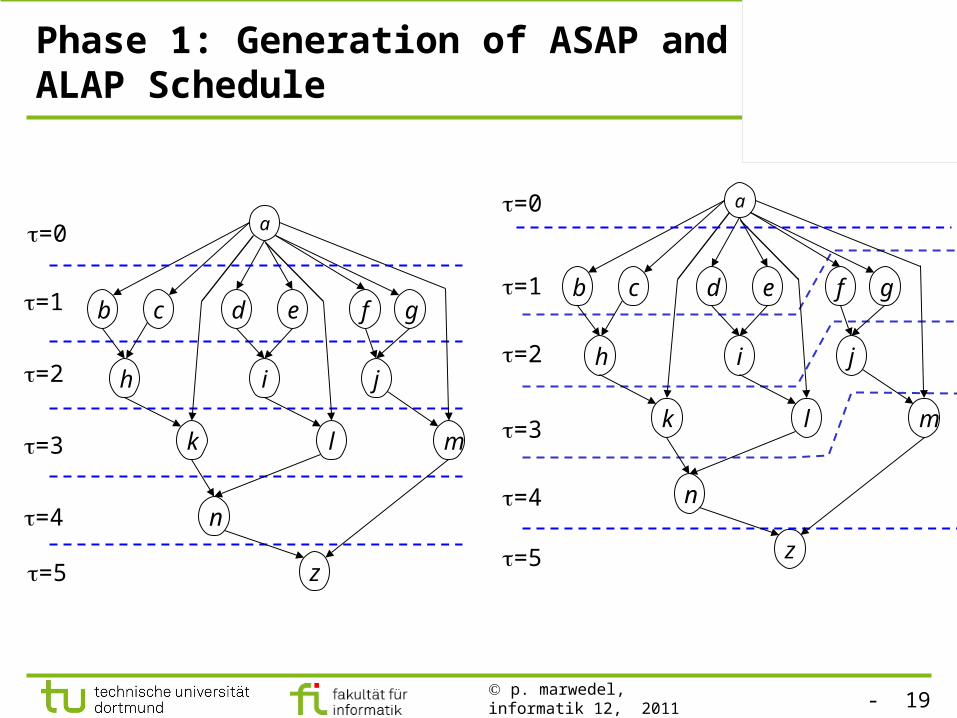
- 19 - p. marwedel, informatik 12, 2011
Phase 1: Generation of ASAP and ALAP Schedule
=1
=2
=3
=4
=5
=1
=2
=3
=4
=5
a
b c d e f g
h i j
k l m
n
z
=0
a
b c d e f g
h i j
k l m
n
z
=0

- 20 - p. marwedel, informatik 12, 2011
Next: computation of “forces”
Direct forces push each task into the direction of lowervalues of D(i).
Impact of direct forces on dependent tasks taken into account by indirect forces
Balanced resource usage smallest forces For our simple example and time constraint=6:
result = ALAP schedule0
1
2
3
4
5
2 31 4 5
i
=1
=2
=3
=4
=5
a
b c d e f g
h i j
k l m
n
z
=0
More precisely …

- 21 - p. marwedel, informatik 12, 2011
1.Compute time frames R(j); 2. Compute “probability“ P(j,i) of assignment j i
R(j)={ASAP-control step … ALAP-control step}
if
0 otherwise

- 22 - p. marwedel, informatik 12, 2011
3. Compute “distribution” D(i)(# Operations in control step i)
P(j,i) D(i)

- 23 - p. marwedel, informatik 12, 2011
4. Compute direct forces (1)
Pi( j,i‘): for force on task j in time step i‘,
if j is mapped to time step i.The new probability for executing j in i is 1;the previous was P ( j, i).
The new probability for executing j in i‘ i is 0; the previous was P (j, i).
i
if
otherwise

- 24 - p. marwedel, informatik 12, 2011
4. Compute direct forces (2)
SF(j, i) is the overall change of direct forces resulting from the mapping of j to time step i.
Example
otherwise
if

- 25 - p. marwedel, informatik 12, 2011
4. Compute direct forces (3)
Direct force if task/operation 1 is mapped to time step 2

- 26 - p. marwedel, informatik 12, 2011
5. Compute indirect forces (1)
DMapping task 1 to time step 2implies mapping task 2 to time step 3
Consider predecessor and successor forces:
Pj, i (j‘,i‘) is the in the probability of mapping j‘ to i‘
resulting from the mapping of j to i
j‘ predecessor of j
j‘ successor of j

- 27 - p. marwedel, informatik 12, 2011
5. Compute indirect forces (2)
Example: Computation of successor forces for task 1 in time step 2
j‘ predecessor of j
j‘ successor of j

- 28 - p. marwedel, informatik 12, 2011
Overall forces
The total force is the sum of direct and indirect forces:
In the example:
The low value suggests mapping task 1 to time step 2

- 29 - p. marwedel, informatik 12, 2011
Overall approach
procedure forceDirectedScheduling;begin
AsapScheduling;AlapScheduling;while not all tasks scheduled do
beginselect task T with smallest total force;schedule task T at time step minimizing forces;recompute forces;
end;end
May be repeated for different task/ processor classes
Not sufficient for today's complex, heterogeneous hardware platforms

- 30 - p. marwedel, informatik 12, 2011
Evaluation of HLS-Scheduling
Focus on considering dependencies
Mostly heuristics, few proofs on optimality
Not using global knowledge about periods etc.
Considering discrete time intervals
Variable execution time available only as an extension
Includes modeling of heterogeneous systems

- 31 - p. marwedel, informatik 12, 2011
Overview
Scheduling of aperiodic tasks with real-time constraints:Table with some known algorithms:
Equal arrival times; non-preemptive
Arbitrary arrival times; preemptive
Independent tasks
EDD (Jackson) EDF (Horn)
Dependent tasks
LDF (Lawler), ASAP, ALAP, LS, FDS
EDF* (Chetto)

- 32 - p. marwedel, informatik 12, 2011
Conclusion
HLS-based scheduling
• ASAP
• ALAP
• List scheduling (LS)
• Force-directed scheduling (FDS)
Evaluation