Mapping color equivalency in a proposed two metric … · Mapping color equivalency in a proposed...

Mapping color equivalency in a

proposed two metric system of color

rendition

Tony EspositoPh.D. Candidate

Penn State University

Department of Architectural Engineering

Overview

Introduction to color rendering

(refresher from previous presentation)

IES TM-30-15 Overview

Rf, Rg, CVG

Dissertation Research

Motivation/Purpose

Methodology

Data

Introduction to analysis

Discussion

2

Color Rendering

https://az616578.vo.msecnd.net/files/responsive/cover/main/desktop/2015/12/31/635871793084619033-1563657366_trippy.jpg

3

Color Rendering: CIE Method

5Tony Esposito | PhD Candidate, Penn State University

CIE General Color Rendering Index (Ra)

The accurate rendition of

color so that they appear

as they would under

familiar (reference)

illuminants

Color Fidelity

Color Rendering: CIE Method


CIE “CRI"


Test Source

Reference Source

CRI only accounts for the magnitude of shift, not direction!

Limitations of considering only fidelity


Perfect Fidelity



CRI = 80 CRI = 80

Increase Saturation

DecreaseSaturation



CRI = 80

CRI = 80

Increase Saturation

DecreaseSaturation

Positive Hue Shift

Negative Hue Shift



Increase Saturation

DecreaseSaturation

Positive Hue Shift

Negative Hue Shift

Constant Fidelity (CRI)



Increase Saturation

DecreaseSaturation

Positive Hue Shift

Negative Hue Shift

Constant Fidelity (CRI)

One metric is not enough!

How many metrics are needed?

14

Preference DiscriminationFidelity

Faithful color rendition in comparison to a reference light source

Rendition of objects such that they appear pleasant or flattering

The ability of a source to reveal slight hue variations of objects (when viewed simultaneously)

Fidelity metric, like CRI Goal: not to quantify individual preference

Most people prefer higher object saturation than achieved under the reference source

Goal: to maximize

How many metrics are needed?

15

Tend to be related to saturation, which can be

quantified with



Rendition of objects such that they appear pleasant or flattering


Fidelity metric, like CRI

gamut area

IES TM-30-15

16

IES Method for Color Rendition

17



Rendition of objects such that they appear pleasant, vivid, or flattering


Rg: A gamut-based metric for prediction of Preference and

Discrimination

Rf: Direct replacement for CRI

IES Method for Color Rendition

18

Fidelity Index (Rf)

The accurate rendition of

color so that they appear

as they would under


illuminants

The average level of

saturation relative to


illuminants.

Gamut Index (Rg)Ranges 0-100 ≈ 60-140 when Rf > 60

Visual description of hue

and saturation changes.

Color Vector Graphic(CVG)

Color Gamut Vector GraphicFidelity

IES TM30 System


Rf

Rg

140

120

130

110

100

90

80

70

6050 60 70 80 90 100

Decreasing Fidelity

Increased Saturation

(on average)

Decreased Saturation

(on average)

Rg > 100

Rg < 100Color Vector Graphic

Shows inc/dec saturation

relative to reference source

Doctoral Work“Mapping color equivalency in a proposed two

metric system of color rendition”

25

Problem

26

60

70

80

90

100

110

120

130

140

50 60 70 80 90 100

Gam

ut

Ind

ex,

Rg

Fidelity Index, Rf

1 2 1

2

Approx. limits for sources on the Planckian locus.

Approx. limits for practical light sources.

Rf-Rg Plot

IES TM-30-15 will not provide:

• Perceptual tradeoffs

• Design recommendations

• Performance thresholds

• Preference suggestions

31

• Fidelity

• Preference

• Discrimination

• CVG

Understand perceptual tradeoffs in the Rf-Rg Space in regards to:

Purpose

Method

How do we do this?

32

Method: CCT

Question: what CCT should be used for

experimentation?

(CCT must be constant)

http://www.banidea.com/wp-content/uploads/2012/09/Lamp-warm-white-day-light-cool-white.jpg

33

Method: CCT

Test: which (practical) CCT can the

TeleLumen most easily achieve?

http://www.banidea.com/wp-content/uploads/2012/09/Lamp-warm-white-day-light-cool-white.jpg

TeleLumen Light Replicator

34

35

MATLAB Simulation

30 million (random) linear combinations of the 16

channels

Keep SPD’s that meet the following

±25K of 3000, 3200, 3500, and 4000K

±0.02 DUV of BBL

Plot Rf/Rg Combinations

Method: CCT

36

Method: CCT

37

Method: CCT

Method

38

CCT 3500 K

Duv 0.000

Rf/Rg

E = 600 lx

70

80

90

100

110

120

130

60 65 70 75 80 85 90 95 100

Gam

ut

Ind

ex,

Rg

Fidelity Index, Rf

Rf-Rg Plot

Method

39

CCT 3500 K

Duv 0.000

Rf/Rg

E = 600 lx

70

80

90

100

110

120

130

60 65 70 75 80 85 90 95 100

Gam

ut

Ind

ex,

Rg

Fidelity Index, Rf

Rf-Rg Plot

Method

40

CCT 3500 K

Duv 0.000

Rf/Rg

E = 600 lx

70

80

90

100

110

120

130

60 65 70 75 80 85 90 95 100

Gam

ut

Ind

ex,

Rg

Fidelity Index, Rf

Rf-Rg Plot

Method

41

CCT 3500 K

Duv 0.000

Rf/Rg

E = 600 lx

70

80

90

100

110

120

130

60 65 70 75 80 85 90 95 100

Gam

ut

Ind

ex,

Rg

Fidelity Index, Rf

Rf-Rg Plot

Method

42

CCT 3500 K

Duv 0.000

Rf/Rg

E = 600 lx

54.1

73.5

78.4

69.8

68.4

77.9

102.4

68.0

55.5

55.0

60.7

112.9

89.7

78.6

102.2

72.0

61.0

80.0

68.1

82.8

88.5

108.9

111.8

131.0

70

80

90

100

110

120

130

60 65 70 75 80 85 90 95 100

Gam

ut

Ind

ex,

Rg

Fidelity Index, Rf

Rf-Rg Plot

Method

43

Rf 65 75 85 95

Rg

120

110

100

90 Y Y Y

80

Apparatus: booth

TeleLumen from above

Mirror for skin evaluations

Consumer products

Real objects (fruit)

Chin rest (for consistency)

44

Apparatus: objects

45

-40

-30

-20

-10

0

10

20

30

40

-40 -30 -20 -10 0 10 20 30 40

b'

a'

Consumer Goods

CocaCola

Orance Crush

Mustard

Sprite

Pepsi

Grape Crush

-40

-30

-20

-10

0

10

20

30

40

-40 -30 -20 -10 0 10 20 30 40b'

a'

Real Fruit

Apple

Orange

LemonApple

Blueberries

Red Onion

Method: participants

46

40 participants

23 male | 17 female

Mean age of 26

12 unique countries

Several unique languages

20

40

240

480

24

12

2

1

x

x

x

x

= 480

= 480

= 480

= 480

# Subjects# Scenes

(per sub.)

# Exp

Sessions

x

x

10

10

(physically can run 10

subjects per day)

10

10

10

10

10

10

10

10

10

10

Combo 1 Combo 2 Combo 3 Combo 4 Combo 5 Combo 6

Combo 7 Combo 8 Combo 9 Combo 10 Combo 11 Combo 12

8 weeks (≈550 hrs) to

completes all sessions

Method: participant structure

53

Method: word choice

Question: what words do we use for

rating scales?

Example:

??

What is “common” vocabulary for describing color?

(we don’t want results to be confounded due to lack of understanding

of vocabulary)

54

Method: word choice

55

Method: word choice

56

Method: final rating scale

Preference

Naturalness

Vividness

Skin

63

Procedure1. Participant enters room

2. Place chin in rest for 2 minutes

3. After 2 minutes, answer survey

• OVERALL survey • Like, Natural, Vivid, Skin

• OBJECT SPECIFIC survey• Like, Natural, Vivid

4. Remove chin rest from booth

5. Administer FM 100 test

• 4 trays, in random Order

http://www.planetecouleur.com/boutique_us/images_produits/fm100-b-z.jpg

64

Results: data points

24 SPD’s x 40 scales (per SPD) x 20 subjects (per SPD) = 19,200 points

Surveys:

Discrimination test:

24 SPD’s x 5 scales (per SPD) x 20 subjects (per SPD) = 2,400 points

19,200

2,400

21,600 total data points

(hand coded)

65

Results: OVERALL “Likeness”

66

Rf 65 75 85 95

Rg

120 4.0 4.3Overall "PREFERENCE" Rating

"Dislike - Like" (Scale 0 - 5)

110 3.5 3.9 3.9 4.3 4.1 4.1

100 3.2 3.9 3.9 3.6 4.1 3.7 4.2 3.7

90 3.2 3.9 3.7 3.5 3.7 3.2

80 2.4 2.5 0.0 5.0

Results: OVERALL “Naturalness”

67

Rf 65 75 85 95

Rg

120 2.4 3.7Overall "NATURALNESS" Rating

"Unnatural - Natural" (Scale 0 - 5)

110 2.3 3.8 3.0 3.9 3.6 3.8

100 2.6 3.8 3.3 3.6 3.5 3.7 4.0 3.6

90 2.6 3.9 3.1 3.3 3.8 3.8

80 2.7 2.7 0.0 5.0

Results: OVERALL “Vividness”

68

Rf 65 75 85 95

Rg

120 4.3 3.8Overall "VIVIDNESS" Rating

"Desaturated - Vivid" (Scale 0 - 5)

110 4.2 3.5 4.0 3.8 4.2 3.7

100 4.0 3.2 3.6 2.8 3.7 2.9 3.4 3.1

90 3.2 3.1 3.3 2.9 3.0 2.6

80 2.7 1.7 0.0 5.0

Results: OVERALL “Likeness” (skin)

69

Rf 65 75 85 95

Rg

120 3.6 3.8Overall "SKIN PREFERENCE" Rating

"Dislike - Like" (Scale 0 - 5)

110 3.5 3.8 3.5 3.8 3.9 4.0

100 3.4 3.1 3.6 3.1 3.7 3.3 3.9 3.6

90 3.2 2.9 3.3 3.3 3.6 2.8

80 2.5 2.0 0.0 5.0

70

Results: FM100 test (Total Error Score)

Rf

Rg

120 56.8 61.8

110 38.2 50.2 33.6 36.4 45.4 36.2

100 36.2 47.2 30 32.4 39 28.8 21.2 20.2

90 43 34.6 38.2 21.2 29.8 36.8

80 39 24.4

65 75 85 95

Farnsworth-Munsell 100 Hue Test

Average Total Error Score (TES)

71

Results: Consider 4 trays in FM100 test

72

Results: FM100 test by tray

73

Results: FM100 test by tray

Discussion: models

74

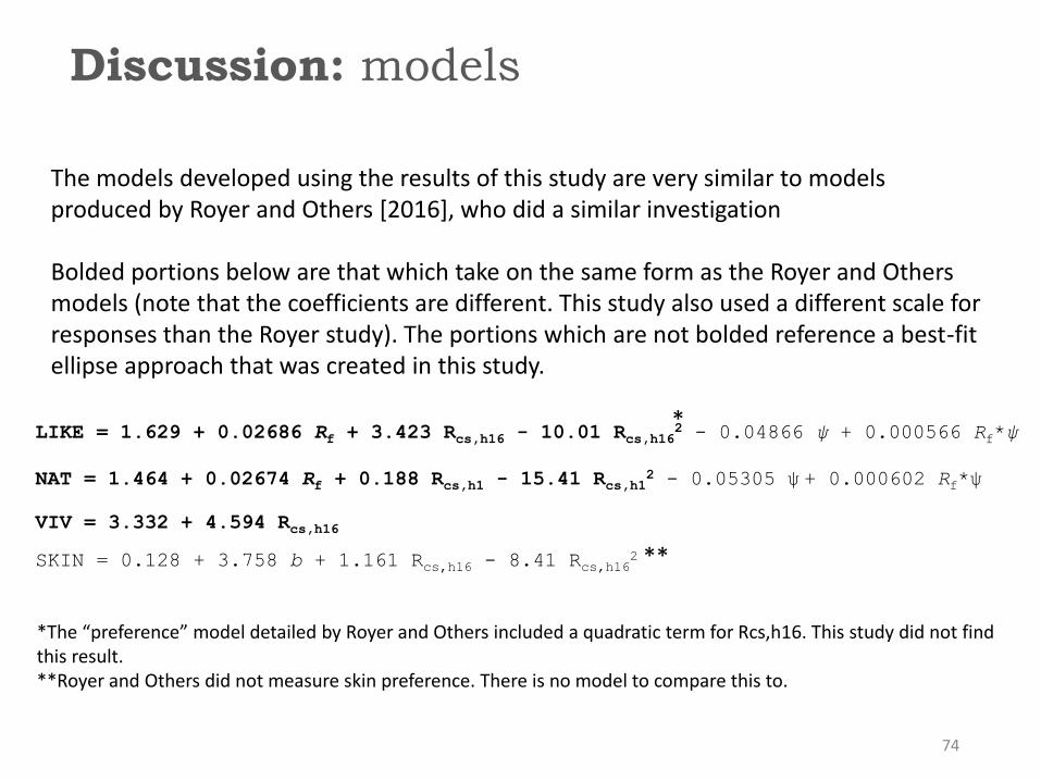
NAT = 1.464 + 0.02674 Rf + 0.188 Rcs,h1 - 15.41 Rcs,h12 - 0.05305 ψ + 0.000602 Rf*ψ

VIV = 3.332 + 4.594 Rcs,h16

LIKE = 1.629 + 0.02686 Rf + 3.423 Rcs,h16 - 10.01 Rcs,h162 - 0.04866 ψ + 0.000566 Rf*ψ

SKIN = 0.128 + 3.758 b + 1.161 Rcs,h16 - 8.41 Rcs,h162

The models developed using the results of this study are very similar to models produced by Royer and Others [2016], who did a similar investigation

Bolded portions below are that which take on the same form as the Royer and Others models (note that the coefficients are different. This study also used a different scale for responses than the Royer study). The portions which are not bolded reference a best-fit ellipse approach that was created in this study.

**

*The “preference” model detailed by Royer and Others included a quadratic term for Rcs,h16. This study did not find this result.**Royer and Others did not measure skin preference. There is no model to compare this to.

*

Discussion: influence of objects

75

4.55.0

3.4

5.5

3.7

4.8

4.24.7

4.13.6

3.1

5.9

1.0

2.0

3.0

4.0

5.0

6.0

7.0

R1 R2 O1 O2 Y1 Y2 G1 G2 B1 B2 P1 P2

Ave

rage

Co

ntr

ibu

tio

n R

atin

g

Object

Co

caC

ola

Can

Ora

nge

Cru

sh C

an

Mu

star

d B

ott

le

Spri

te C

an

Pep

si C

an

Gra

pe

Cru

sh

Red

Ap

ple

Ora

nge

Lem

on

Gre

en A

pp

le

Blu

eber

ries

On

ion

Leas

tM

ost

0

5

10

15

20

25

30

35

40

R1 R2 O1 O2 Y1 Y2 G1 G2 B1 B2 P1 P2

Co

un

t

Object

Number of times ranked in top 3

Co

caC

ola

Can

Ora

nge

Cru

sh C

an

Mu

star

d B

ott

le

Spri

te C

an

Pep

si C

an

Gra

pe

Cru

sh

Red

Ap

ple

Ora

nge

Lem

on

Gre

en A

pp

le

Blu

eber

ries

On

ion

Discussion: Color Vector Graphic

77

The CVG is simple to interpret, but numerically complex

It’s complexity does not lend itself to use in specification

The best-fit ellipse approach is a simpler method to describe the CVG

All best-fit models include metrics extracted from the CVG (Rcs,hi or ellipse parameters)

The CVG is not supplementary information!

Discussion: FM100

78

Discussion: FM100

79

Discussion: FM100

80

Metrics based on traditional ideas (e.g. fidelity and gamut) are not strong predictors of error score

We need to build custom metrics that directly reflect what is happening to color chips in color space

New metrics are proposed based on the concepts that:

1. Chips which are close together will be harder to distinguish (thus increasing error score)

2. That light sources which transpose color in color space will cause significant errors

The model built with metrics based on these underlying concepts is stronger than models than can be built with fidelity and gamut measures.

Summary

81

An experiment was performed which systematically varied Rf, Rg, and CVG orientation

Subjective ratings of preference, naturalness, and vividness were recorded

Color discrimination was also measured (FM100 hue test)

Best-fit ellipses were developed to quantify the CVG

Models (generally) agree with those proposed by Royer and Others [2016]

Custom color discrimination metrics were used to create models which are generally stronger than models built with average fidelity and gamut measures.

Analysis shows that it is important to consider the magnitude of object shifts when making inferences on participant rating strategies.

82TH

AN

K Y

OU

83

Questions?

Tony EspositoPh.D. Candidate

Penn State University

Department of Architectural Engineering

Mapping color equivalency in a proposed two metric … · Mapping color equivalency in a proposed...

Documents

Transcript of Mapping color equivalency in a proposed two metric … · Mapping color equivalency in a proposed...