Mapping Bedrock Topography of the Portage and Schoolcraft ...

Western Michigan University Western Michigan University

ScholarWorks at WMU ScholarWorks at WMU

Master's Theses Graduate College

4-2018

Mapping Bedrock Topography of the Portage and Schoolcraft NW Mapping Bedrock Topography of the Portage and Schoolcraft NW

7.5’ Quadrangles, Kalamazoo Co. MI, Using the HVSR Passive 7.5’ Quadrangles, Kalamazoo Co. MI, Using the HVSR Passive

Seismic Method Seismic Method

Benjamin B. Seiderman

Follow this and additional works at: https://scholarworks.wmich.edu/masters_theses

Part of the Geology Commons, Geophysics and Seismology Commons, and the Glaciology Commons

Recommended Citation Recommended Citation Seiderman, Benjamin B., "Mapping Bedrock Topography of the Portage and Schoolcraft NW 7.5’ Quadrangles, Kalamazoo Co. MI, Using the HVSR Passive Seismic Method" (2018). Master's Theses. 3401. https://scholarworks.wmich.edu/masters_theses/3401

This Masters Thesis-Open Access is brought to you for free and open access by the Graduate College at ScholarWorks at WMU. It has been accepted for inclusion in Master's Theses by an authorized administrator of ScholarWorks at WMU. For more information, please contact [email protected].

http://scholarworks.wmich.edu/


https://scholarworks.wmich.edu/

https://scholarworks.wmich.edu/masters_theses

https://scholarworks.wmich.edu/grad

https://scholarworks.wmich.edu/masters_theses?utm_source=scholarworks.wmich.edu%2Fmasters_theses%2F3401&utm_medium=PDF&utm_campaign=PDFCoverPages

http://network.bepress.com/hgg/discipline/156?utm_source=scholarworks.wmich.edu%2Fmasters_theses%2F3401&utm_medium=PDF&utm_campaign=PDFCoverPages



https://scholarworks.wmich.edu/masters_theses/3401?utm_source=scholarworks.wmich.edu%2Fmasters_theses%2F3401&utm_medium=PDF&utm_campaign=PDFCoverPages

mailto:[email protected]



MAPPING BEDROCK TOPOGRAPHY OF THE PORTAGE AND SCHOOLCRAFT NW 7.5’

QUADRANGLES, KALAMAZOO CO. MI, USING THE HVSR PASSIVE

SEISMIC METHOD

by


A thesis submitted to the Graduate College

in partial fulfillment of the requirements

for the degree of Master of Science

Geosciences

Western Michigan University

April 2018

Thesis Committee:

Alan E. Kehew, Ph.D., Chair

William A. Sauck, Ph.D.

Robb Gillespie, Ph.D.

Copyright by


2018

MAPPING BEDROCK TOPOGRAPHY OF THE PORTAGE AND SCHOOLCRAFT NW 7.5’

QUADRANGLES, KALAMAZOO CO., MI, USING THE HVSR PASSIVE

SEISMIC METHOD

Benjamin B. Seiderman, M.S.

Western Michigan University, 2018

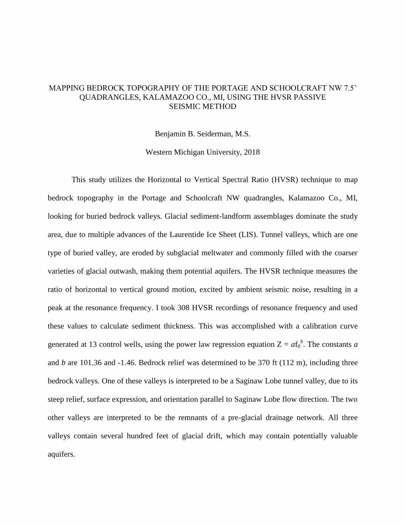
This study utilizes the Horizontal to Vertical Spectral Ratio (HVSR) technique to map

bedrock topography in the Portage and Schoolcraft NW quadrangles, Kalamazoo Co., MI,

looking for buried bedrock valleys. Glacial sediment-landform assemblages dominate the study

area, due to multiple advances of the Laurentide Ice Sheet (LIS). Tunnel valleys, which are one

type of buried valley, are eroded by subglacial meltwater and commonly filled with the coarser

varieties of glacial outwash, making them potential aquifers. The HVSR technique measures the

ratio of horizontal to vertical ground motion, excited by ambient seismic noise, resulting in a

peak at the resonance frequency. I took 308 HVSR recordings of resonance frequency and used

these values to calculate sediment thickness. This was accomplished with a calibration curve

generated at 13 control wells, using the power law regression equation Z = af0b. The constants a

and b are 101.36 and -1.46. Bedrock relief was determined to be 370 ft (112 m), including three

bedrock valleys. One of these valleys is interpreted to be a Saginaw Lobe tunnel valley, due to its

steep relief, surface expression, and orientation parallel to Saginaw Lobe flow direction. The two

other valleys are interpreted to be the remnants of a pre-glacial drainage network. All three

valleys contain several hundred feet of glacial drift, which may contain potentially valuable

aquifers.

ii

AKNOWLEDGEMENTS

First I would like to thank Dr. Sauck and Director John Yellich of the Michigan

Geological Survey for approaching me with the Portage Bedrock Mapping project, and for

funding a large portion of my research. This opportunity led me to my eventual research focus.

I would also like to thank Sita Karki and Scott Feldpausch for their assistance and

guidance using ArcMap GIS, and helping me with understanding and processing the HVSR data.

I want to thank my family for their continued love and support during my education, as

well as all the friends I have made in Kalamazoo along the way.

Finally, I would like to thank my advisor, Dr. Kehew, for all of his help, guidance, and

patience during the implementation of this project.


iii

TABLE OF CONTENTS

AKNOWLEDGEMENTS............................................................................................................ ii

LIST OF TABLES ........................................................................................................................ v

LIST OF FIGURES .....................................................................................................................vi

CHAPTER

I. INTRODUCTION ................................................................................................ 1

Study Area ...................................................................................................... 1

Bedrock Geology ............................................................................................ 5

Surficial Geology ............................................................................................ 5

The HVSR Method ......................................................................................... 8

II. REVIEW OF LITERATURE ............................................................................. 12

Tunnel Valleys .............................................................................................. 12

HVSR Studies ............................................................................................... 16

III. METHODS ......................................................................................................... 19

Equipment ..................................................................................................... 19

Surveying Technique .................................................................................... 19

Data Processing ............................................................................................. 20

Calibration..................................................................................................... 26

Mapping and Interpolation ............................................................................ 27

IV. RESULTS ........................................................................................................... 28

iv

Table of Contents – Continued

CHAPTER

HVSR Data ................................................................................................... 28

Bedrock Topography and Glacial Drift Thickness ....................................... 31

Cross Sections ............................................................................................... 34

V. DISCUSSION ..................................................................................................... 39

Bedrock Valleys ............................................................................................ 39

Quality of HVSR Data .................................................................................. 43

HVSR Sources of Error ................................................................................ 45

VI. CONCLUSIONS................................................................................................. 51

REFERENCES ........................................................................................................................... 53

APPENDICES ............................................................................................................................ 56

A. HVSR Data ..................................................................................................................... 56

v

LIST OF TABLES

1. Calibration curve HVSR data ......................................................................................... 43

2. Al Sabo Land Preserve error recordings ......................................................................... 47

3. Wood Hall error recordings ............................................................................................ 48

4. Three-hour recording ...................................................................................................... 49

vi

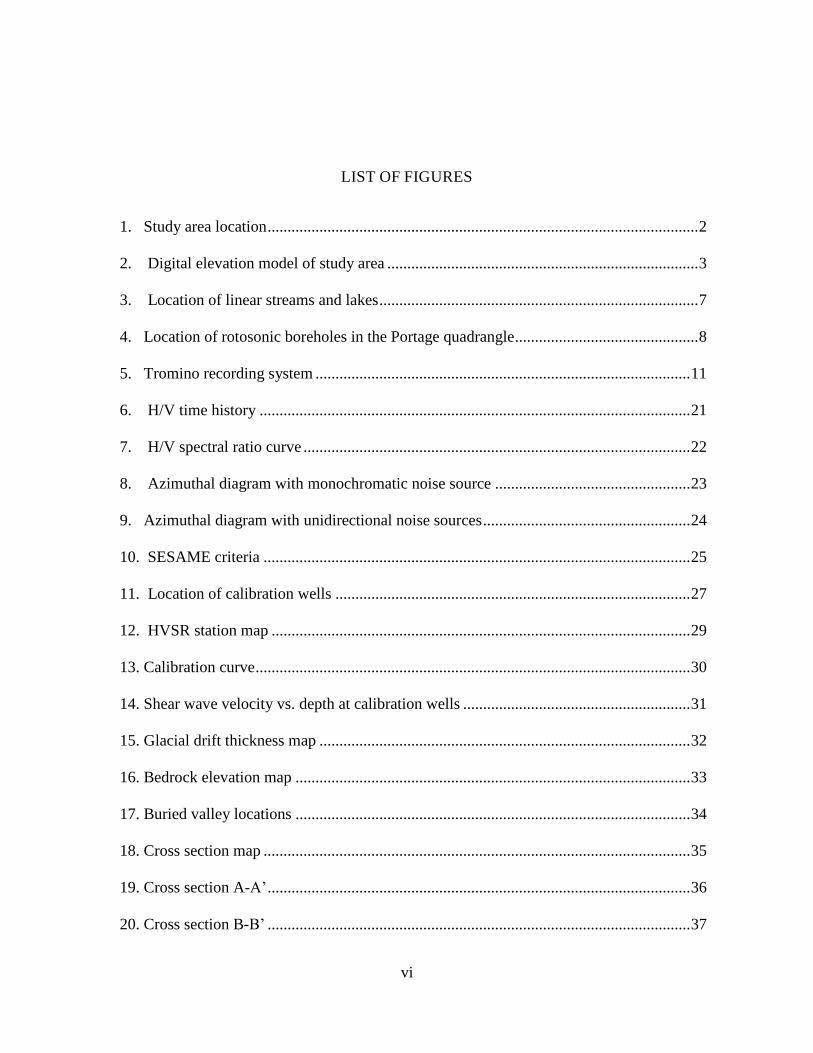
LIST OF FIGURES

1. Study area location ............................................................................................................ 2

2. Digital elevation model of study area .............................................................................. 3

3. Location of linear streams and lakes ................................................................................ 7

4. Location of rotosonic boreholes in the Portage quadrangle .............................................. 8

5. Tromino recording system .............................................................................................. 11

6. H/V time history ............................................................................................................ 21

7. H/V spectral ratio curve ................................................................................................. 22

8. Azimuthal diagram with monochromatic noise source ................................................. 23

9. Azimuthal diagram with unidirectional noise sources .................................................... 24

10. SESAME criteria ........................................................................................................... 25

11. Location of calibration wells ......................................................................................... 27

12. HVSR station map ......................................................................................................... 29

13. Calibration curve ............................................................................................................. 30

14. Shear wave velocity vs. depth at calibration wells ......................................................... 31

15. Glacial drift thickness map ............................................................................................. 32

16. Bedrock elevation map ................................................................................................... 33

17. Buried valley locations ................................................................................................... 34

18. Cross section map ........................................................................................................... 35

19. Cross section A-A’ .......................................................................................................... 36

20. Cross section B-B’ .......................................................................................................... 37

vii

List of Figures – Continued

21. Cross section C-C’ .......................................................................................................... 38

22. Bedrock and surface valleys ........................................................................................... 40

23. Low frequency noise HVSR curve ................................................................................. 45

1

CHAPTER I

INTRODUCTION

Study Area

The Portage and Schoolcraft NW 7.5’ quadrangles are located in the SW corner of

Kalamazoo County, Michigan (Figure 1). These quadrangles were selected to assess

groundwater resources for the City of Portage. There are numerous linear surface depressions

located in both quadrangles, possibly indicative of bedrock valleys. Many of these depressions

contain surface water bodies, such as lakes and streams, which are visible on available digital

elevation models (DEM) of the county. The study area for this project consists of a lowland

situated in the middle of a complex, interlobate moraine system which includes both the

Kalamazoo and Sturgis moraines and the Tekonsha upland. (Figure 2).These sediment-landform

assemblages reflect interactions between the Lake Michigan Lobe and the Saginaw Lobe of the

Laurentide Ice Sheet (LIS). The Kalamazoo moraine contains the highest elevations in

southwestern Michigan, and the Tekonsha upland lies approximately fifteen miles to the east.

2

Figure 1. The study area includes both Schoolcraft NW and Portage Quadrangles.

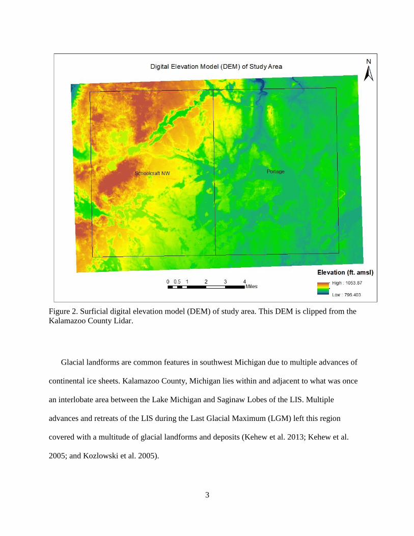
3

Figure 2. Surficial digital elevation model (DEM) of study area. This DEM is clipped from the

Kalamazoo County Lidar.

Glacial landforms are common features in southwest Michigan due to multiple advances of

continental ice sheets. Kalamazoo County, Michigan lies within and adjacent to what was once

an interlobate area between the Lake Michigan and Saginaw Lobes of the LIS. Multiple

advances and retreats of the LIS during the Last Glacial Maximum (LGM) left this region

covered with a multitude of glacial landforms and deposits (Kehew et al. 2013; Kehew et al.

2005; and Kozlowski et al. 2005).

4

Tunnel valleys are subglacial bedforms attributed to erosion by subglacial meltwater (O’

Cofaigh 1996). After erosion, which may or may not incise downward into bedrock, these

valleys can then be infilled with sediment, ice, and debris during glacial retreat. There are many

hypotheses to explain the mechanism behind tunnel valley formation. Additionally, recent

geophysical techniques can be employed to ascertain their location and distribution if they incise

into bedrock. The Horizontal to Vertical Spectral Ratio method, also known as Nakamura’s

method (Nakamura, 1989), can be used to determine the resonance frequency of the sediment

layer. It is a passive-seismic method, which does not require a user-generated seismic

disturbance. This method measures the ratio of the frequency spectra of horizontal to vertical

ground motion, resulting in a graphic peak at the resonance frequency. This peak frequency can

be used to determine the thickness of sediment overlying bedrock if the shear wave velocity (Vs)

is known, utilizing the relationship between sediment thickness (H) and resonance frequency,

given by the equation: f0 = Vs/4H.

This project demonstrates the usefulness of the passive-seismic method in acquiring and

processing data necessary to locate and identify natural resources. Bedrock valleys represent

possible water resources. Unconsolidated glacial outwash is an ideal medium for containing

aquifers, due to the high availability of pore space. Tunnel valleys commonly contain the more

coarse-grained varieties of glacial outwash, such as chaotic assemblages of glaciofluvial and

glaciolacustrine sands and gravels (O’ Cofaigh 1996). Therefore, it is likely that these features

contain potentially productive aquifers. Hence, it is beneficial to delineate bedrock valleys for

groundwater exploration. The HVSR method, which is an inexpensive, non–invasive method, is

an ideal method for mapping the bedrock surface and gathering data, especially for any area

devoid of hydrologic or subsurface data.

5

The objective of this project was to conduct a passive seismic survey of both the

Schoolcraft NW and Portage quadrangles using the HVSR method in order to detail and interpret

the bedrock topography, in particular to identify and locate any glacial tunnel valleys that may

incise into the bedrock topography.

Bedrock Geology

The Paleozoic bedrock located throughout the study area consists of Mississippian-age

Coldwater Shale, which dips gently NE towards the center of the Michigan Basin. Rieck and

Winters, 1979, noted that the surface topography of glaciated areas can be influenced by the

underlying bedrock. Pre-glacial stream valleys often fill with ice blocks that later become buried.

The ice blocks then slowly melt due to the insulation of outwash either caved in from the valley

sides or deposited during retreat, and may eventually become surface valleys. The contact

between the Coldwater shale and the glacial drift is critical to this study. Furthermore, the

impedance contrast between the glacial drift and the Coldwater Shale is an important variable in

determining the quality of the recording, and hence the precision of the resonance peak. The

minimum acoustic impedance ratio of the bedrock and the overlaying sediment layer must be

greater than 2:1 in order for the HVSR method to be effective (Lane et al. 2008).

Surficial Geology

Both the Portage and Schoolcraft NW quadrangles are located in Kalamazoo County,

Michigan (Figure 1). This area is located near what was once a boundary between two lobes of

the LIS, the Lake Michigan Lobe and the Saginaw Lobe (Kehew et al., 2013). The Saginaw Lobe

at one point during the Late Glacial Maximum occupied most of southwest Michigan. Much of

the current surface topography was produced when the Saginaw Lobe stagnated during its retreat

6

through this area. Tunnel valleys have been mapped within this region (Kehew et al., 2013,

Kehew et al., 2012, Kehew et al., 2005). There is evidence to suggest the movements of these

two lobes after the LGM, along with the Huron-Erie lobe to the east, may have been

asynchronous. This is supported by the presence of tills and outwash deposited over tunnel

valleys located in the land systems formed by the Saginaw Lobe (Kehew et al., 2013). Although

it is currently unknown how many previous advances of the Saginaw Lobe have occurred, burial

of surficial features deposited in the study area beneath glacial outwash during the retreat of the

Lake Michigan Lobe was likely.

The dominant surface geology of the Portage quadrangle consists of broad outwash fans

that emanated from the Lake Michigan Lobe. They extend east and gently grade from the

Kalamazoo Moraine (Kehew et al., 2005). Municipal water well data acquired from the

Michigan Geographic Database Library characterize the local surface geology as primarily sand

and gravel, with some interbedded clay layers.

The Schoolcraft NW quadrangle is situated directly west of the Portage quadrangle. The

western border of the quadrangle includes part of the Kalamazoo Moraine, which has the highest

elevations within the study area, and the most prominent surficial glacial feature. East of the

Kalamazoo moraine is a broad lowland that extends east into the Portage quadrangle. The

dominant lithology, based on well log data from the Michigan Geographic Database Library, is

the same as the Portage Quadrangle: It is primarily gravel and sand with interbedded layers of

clay and diamicton. This lowland is dotted with numerous kettle lakes and streams, which follow

linear surface depressions (Figure 3).

7

Figure 3. DEM of study area. Linear chains of lakes and streams are outlined by heavy dashed

lines.

The lowland within which the study area is located contains several of these lake

assemblages. Previous work in this area has interpreted them to be palimpsest tunnel valleys,

formed during the advance of the Saginaw Lobe during the LGM, and buried by outwash during

its retreat (Kehew et al. 1999). Four rotosonic boreholes were drilled in the Portage quadrangle

in 2003 to investigate if an incised tunnel valley was located beneath this trend of lakes (Figure

4).

8

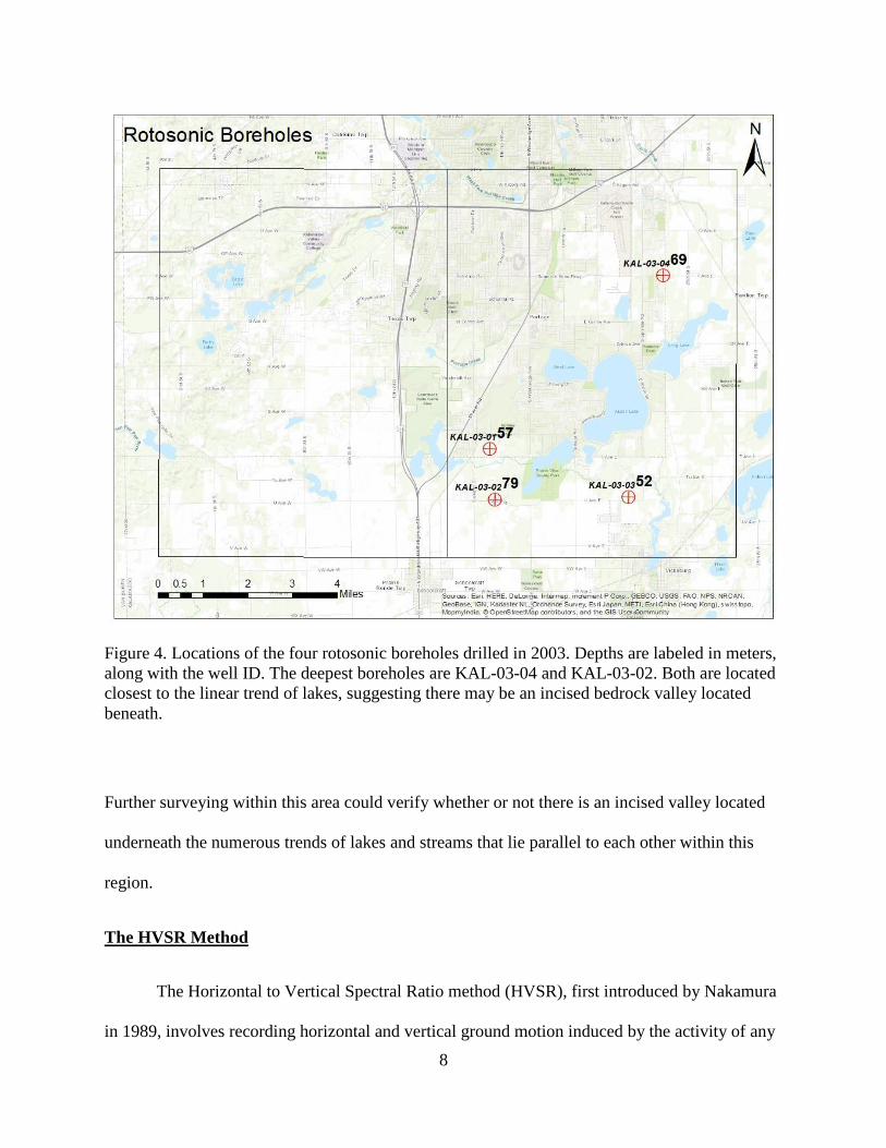
Figure 4. Locations of the four rotosonic boreholes drilled in 2003. Depths are labeled in meters,

along with the well ID. The deepest boreholes are KAL-03-04 and KAL-03-02. Both are located

closest to the linear trend of lakes, suggesting there may be an incised bedrock valley located

beneath.

Further surveying within this area could verify whether or not there is an incised valley located

underneath the numerous trends of lakes and streams that lie parallel to each other within this

region.

The HVSR Method

The Horizontal to Vertical Spectral Ratio method (HVSR), first introduced by Nakamura

in 1989, involves recording horizontal and vertical ground motion induced by the activity of any

9

and all seismic waves. The method uses the spectral ratio of horizontal to vertical ground motion

to calculate the resonance frequency of sediment overlaying bedrock. Resonance frequency is the

frequency at which a system oscillates at enhanced amplitude, due to an external driving force.

In this case, the frequency of sediment oscillations is driven by ambient seismic waves (also

termed microtremors) which are ubiquitous in the subsurface (Nakamura, 1989). A number of

forces, both natural and anthropogenic, cause these microtremors. Examples of natural causes

include the movement of ocean and lake swells and waves, wind, and the teleseisms of distant

earthquakes. Anthropogenic sources may include traffic, pumping of water wells, or drilling for

oil or gas. Seismic waves caused by natural sources typically exhibit low frequencies (0.003 –

0.5 Hz) whereas seismic waves caused by anthropogenic sources are typically higher frequency

(>1.0 Hz).

The HVSR method estimates resonance frequency by combining the two horizontal

spectra (N-S and E-W) and then dividing this result, point by point, by the spectrum of the

vertical motion. The HVSR instrument records the three components of ground motion for the

chosen period, then calculates the spectral H/V ratio during post-processing. The contact

between sediment and bedrock is what makes the resonance phenomenon possible in a two-layer

system of loose unconsolidated sediment over lithified bedrock; this is due to the difference in

shear wave acoustic impedance between the upper soft layer and the bedrock (Seht and

Wolhenberg, 1999; Lane et al. 2008; Chandler and Lively 2014; Johnson and Lane 2016).

Acoustic impedance is the product of shear wave velocity and density for a given layer. Acoustic

impedance ratio in geologic terms refers to the difference in shear wave velocity in different

lithologic units, based on the rigidity modulus, which controls shear wave velocity. In order for

the HVSR method to be effective, this ratio must be greater than 2.5:1. The fundamental

10

relationship between sediment thickness and resonance frequency in a uniform two-layer case is

described by the equation Z = Vs/4f0, where Z is thickness of the surface layer, f0 is the

resonance frequency, and Vs is the average shear wave velocity to the base of that layer (Lane

and Johnson 2008). Average shear wave velocity of a layer increases with compaction and

cementation; this occurs as the thickness of the layer increases. Glacial sediments deposited over

many cycles of glaciation tend to become indurated by repeated subglacial compaction and

deposition, and increased overburden in the form of younger sediment. Therefore, because the

study area displays a wide range of overburden thicknesses, using a constant value for Vs is not

appropriate. Instead, a non-linear graph of sediment thickness (H) vs resonance frequency (f0)

can be made from readings taken at calibration wells where bedrock depths are known.

Converting the two axes of the graph to log scales generally produces a distribution of points that

can be fit with a straight line of best fit. The equation of this line is in the form of the power law:

Z = af0b (Lane et al. 2008), where Z is thickness of the surface layer, f0 is the resonance

frequency, a is the intercept of the line with the vertical axis whose coordinate is 1.00, and b is

the slope of the line. This power law equation relates the change in Vs observed as both depth

and compaction of glacial drift increases.

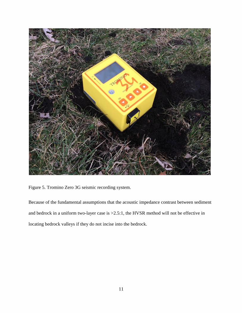
Instruments, such as the Guralp and the Tromino, measure the H/V spectrum of seismic

background noise. The Tromino (Figure 5) is a three-component broadband seismometer (Moho

Science & Technology). The three components measured are north-south, east-west, and vertical.

11

Figure 5. Tromino Zero 3G seismic recording system.

Because of the fundamental assumptions that the acoustic impedance contrast between sediment

and bedrock in a uniform two-layer case is >2.5:1, the HVSR method will not be effective in

locating bedrock valleys if they do not incise into the bedrock.

12

CHAPTER II

REVIEW OF LITERATURE

Tunnel Valleys

Tunnel valleys are characteristic features of glacial landscapes that have been discussed

for more than a century. They have long, undulating, convex-upward profiles that are oriented

parallel to glacier flow lines, terminate near former ice margins, often at the heads outwash fans,

and often occur in association with other subglacial landforms (Kehew et al. 2012). Despite this

consensus, little agreement exists concerning the origin of tunnel valleys. Many possible

mechanisms for their formation have been posited (Gao 2011; Hooke and Jennings 2006; Huuse

and Lykke-Anderson 2000; Jørgensen and Sandersen 2006; Kehew et al. 2012; Ó’ Cofaigh

1996). These hypotheses generally invoke subglacial meltwater as the main agent of tunnel

valley formation in models that include (1) steady-state formation by low-pressure meltwater, (2)

catastrophic outbursts of subglacial meltwater in discrete, high-pressure subglacial conduits, (3)

episodic outbursts of low to moderate magnitude, (4) time-transgressive formation behind a

retreating ice margin, and (5) composite valleys formed over multiple glacial cycles (Kehew et

al. 2012).

Steady-state formation by low-pressure meltwater

Physical properties of the glacier substrate are critical when considering sediment

deformation at the magnitude of tunnel valley erosion. Studies of the ice-bed-interface between

glaciers and their substrates show a distinction exists between hard, strain-resistant beds, and

soft, deformable beds (Boulton et al. 2001; Altuhafi et al. 2010). Boulton and Hindmarsh (1987)

propose the formation of tunnel valleys through steady state removal of sediment by subglacial

meltwater, flowing at low pressures through R-channels, which are subglacial conduits that

13

incise upwards into the glacier ice (Benn and Evans, 2010). One the meltwater begins to erode

into the substrate they become known as N-channels. For this model to work, the bed of the

glacier must be composed of soft deformable sediment that can creep into these N-channels due

to basal pressure differences. Meltwater can then flush them from the drainage system. However,

a shortcoming of this theory is that it cannot account for tunnel valleys that incise into bedrock

(O’ Cofaigh, 1996). In addition, other drainage systems can convey subglacial meltwater flow.

These include linked cavity networks, braided canal networks, groundwater flow, and water

films (Benn and Evans 2010).

Catastrophic outbursts of subglacial meltwater in discrete, high-pressure subglacial conduits

The catastrophic outburst theory for tunnel valley formation refers to the release of

impounded subglacial meltwater behind a glacial barrier, such as an ice margin, moraine, or

permafrost wedge. The main source of evidence for this theory comes from the genetic

relationship between tunnel valleys and other subglacial landforms and erosional features, such

as eskers (Cofaigh, 1996; Kehew et al. 2012). Hooke and Jennings (2006) proposed a model in

which reservoirs of meltwater, which may be englacial or subglacial, build up behind a barrier

complex. This barrier could be a frozen wedge of permafrost, moraine, or an ice barrier. The

barrier is sufficient to prevent escape of meltwater through intergranular flow in the sediment

substrate, braided systems, or other types of distributed drainage systems. As the reservoir of

meltwater builds up, pressure on the barrier increases until a breach develops, and the

accumulated meltwater bursts forth under high pressure through a small conduit. One possible

cause of catastrophic outbursts could be piping towards the ice margin. The high potential

gradient that develops within the ice-bed-interface creates an erosional cavity. This cavity has

lower pressure than at the ice-bed-interface, which forces water into the cavity, eroding through

14

the substrate (Hooke and Jennings 2006). Headward piping from the ice margin would be

required to tap into the interior of the reservoir, which would maintain the outburst flow. This

model explains the erosion of a tunnel valley during a single event.

Catastrophic outbursts of meltwater may also occur as massive sheet floods. These events

are hypothesized to have formed most types of subglacial landforms, including tunnel valleys,

eskers, and drumlins (Shaw, 1989; Shaw 2010, Fisher et al. 2005). This mechanism requires the

accumulation of meltwater in a massive subglacial lake, ponded by either a permafrost margin or

moraine. Failure of the impoundment results in the release of an enormous flood up to hundreds

kilometers wide. As the velocity of flow wanes, the sheet flood collapses into channelized flow

that can erode tunnel valleys (Brennand and Shaw, 1994; Fisher et al. 2005).

Episodic outbursts of low to moderate magnitude

Despite occurring at a lower magnitude than catastrophic outbursts, the episodic

discharge of meltwater at low to moderate magnitudes is another hypothesis for the formation

tunnel valley formation (Kehew et al., 2012; Jørgensen and Sanderson, 2006). Jørgensen and

Sanderson (2006) describe several series of buried and open tunnel valleys in Denmark. They

concluded that multiple advances and retreats of the Scandinavian Ice Sheet eroded several

generations of tunnel valleys, based on cut-and-fill structures, crosscutting relationships between

tunnel valley fills, and the overlapping pattern of open tunnel valleys superimposed on top of

buried bedrock valleys. Evidence for periodic outbursts include (1) boulder accumulations in fan

deposits associated with tunnel valleys, (2) the anastomosing nature of tunnel valley systems,

and (3), presence of bedforms associated with subglacial meltwater flow. Hooke and Jennings

(2006) applied this hypothesis to tunnel valleys located in Wisconsin and Minnesota at the

15

southern margin of the Laurentide Ice Sheet during formation. This model assumes extensive

permafrost proximal to the margin, which impounds subglacial meltwater.

Time-transgressive formation behind a retreating ice margin

Time transgressive formation of tunnel valleys refers to the formation of tunnel valleys

behind a retreating margin of a glacier (O’ Cofaigh, 1996). As the glacier retreats, tunnel valleys

form at or directly behind the margin by way of periodic outbursts. Headward erosion of the

tunnel valley towards the interior reservoir can take place as the glacier margin retreats (Kehew

et al., 2012). Very long tunnel (6 – 30 km) valleys continue to form behind the margin through

headward erosion.

Composite valleys formed over multiple glacial cycles

Composite valleys form as numerous glacial advances and retreats exploit erosional

features already present in the landscape. As glaciers advance, it is possible for existing valleys

to be re-occupied; in some cases open tunnel valleys can form above or cut through other

previous valleys. Tunnel valleys formed this way are known as palimpsest tunnel valleys (Kehew

et al., 2012). Jørgensen and Sanderson (2006) examined tunnel valleys located in the Danish

North Sea. Although one of the proposed mechanisms of tunnel valley formation for this area is

periodic outbursts of low to moderate magnitude, they also identified at least four generations of

tunnel valleys, by evaluating crosscutting relationships between the valleys, and the presence of

multiple cut-and-fill structures. In southwest Michigan, several palimpsest tunnel valleys evolved

through interactions between the Saginaw and Lake Michigan lobes of the Laurentide Ice Sheet

(Kehew et al. 2012). After erosion and filling with ice and debris by the Saginaw Lobe, they

16

were overridden or buried by sediment deposited by the Lake Michigan Lobe, forming

palimpsest tunnel valleys. Gently sloping outwash fans dip toward the east from the Lake

Michigan Lobe ice margin position, denoted by the Kalamazoo moraine. When the lobes

retreated, melting of the buried ice exhumed the Saginaw Lobe valleys.

HVSR Studies

Although the HVSR method is relatively recent, first appearing in 1989, it has become an

active field of study, useful in conjunction with other surveying techniques to collect hydrologic

and seismic data. For example, Seht and Wohlenberg (1999) evaluated sediment thicknesses in

the Lower Rhine Embayment of Germany using the HVSR method. This study is based on 102

recordings, with thirty-four recordings made within close proximity to drilling sites that reached

bedrock. These thirty-four calibration sites were used to plot resonance frequency against

sediment thickness, using a power law expression with constants “a” = 96 and “b” = -1.388. The

calculated sediment thicknesses were compared with refraction seismic cross sections mapped

through the study area. The bedrock profile generated by the survey correlated well with the

refraction cross-sectional values.

Gosar and Lenart (2009) evaluated sediment thickness in the Ljubljana Moor basin of

Slovenia using the HVSR method. The Ljubljana Moor basin is filled with varying amounts of

fluvial and lacustrine sediment, ranging in thickness from 0 – 200 m. These deposits overlay

Paleozoic bedrock, consisting of sandstones and shales. This survey utilized 53 HVSR

measurements, taken at boreholes that reached bedrock to identify the resonance frequency. This

frequency was then plotted with the known bedrock depths using a power law regression,

resulting in power law coefficients of “a” = 105.5 and “b” = -1.25. They also conducted a

17

seismic refraction survey along a 16km-long transect through the entire Ljubljana Moor basin.

They then applied the HVSR method to the same transect at 64 locations spaced 250m apart in

order to compare sediment thicknesses recorded by both methods. The results of this study

showed strong similarities between the thicknesses calculated using both the seismic refraction

survey and the HVSR method.

Haefner et al. (2010) applied the HVSR method in Franklin County, OH to determine

sediment thicknesses within the South Well Field (SWF). The study area for this project is also a

two-layer system of glacial drift and Devonian-age Ohio Shale, similar to the Portage, Michigan

area. For this study, both a site-specific regression equation and a published regression were used

to calculate sediment thickness. Using the site-specific regression equation, they observed a

mean difference of 14.2% between known and calculated sediment thicknesses at the control

wells.

Chandler and Lively (2014) have applied the HVSR method in Minnesota to determine

the thickness of Quaternary glacial deposits in three locations: (1) the Twin Cities metropolitan

area, (2) south-central Minnesota, and (3) the terrace and floodplain deposits in southeastern

Minnesota and adjacent sections of Wisconsin. They used over 35 control wells to generate

regional calibration curves for each study area. Effective results were acquired in the Twin Cities

metro area, where the underlying basement rock is composed of rigid Paleozoic sedimentary

rock cut by many igneous and metamorphic intrusions. However, in central and eastern

Minnesota, the bedrock geology consists of much softer saprolith, developed on top of

Precambrian rocks. The presence of this softer layer led to results that were more incoherent.

They concluded that the HVSR method is most effective in a two-layer scenario, with a strong

impedance contrast.

18

Guillier et al. (2006) applied the HVSR method to evaluate resonance frequency peaks

over different site structures, such as steep and gentle slopes, valley edges and sides, and flat

surfaces. They found that H/V peaks are more reliable and sharp when the bottom layer in a 2-

layer system is flat. The depth to bedrock may be overestimated if a recording is taken on a steep

slope. They associated sloping and steep surfaces with broad, plateau-shaped H/V curves. Flat

surfaces with a >2:1 impedance contrast yielded sharper H/V curves.

The HVSR method was also applied in Michigan. Students at Western Michigan

University have undertaken projects involving the HVSR method (Feldspausch, 2017,

VanderMeer, 2017). Feldpausch (2017) used the HVSR method jointly with gravity methods to

determine the bedrock topography of the Dowling and Maple Grove quadrangles, Barry County,

Michigan.

VanderMeer (2017) used the HVSR method in conjunction with high resolution LiDAR

and auger sampling to characterize the glacial geologic history for Pictured Rocks National

Lakeshore, Michigan. This investigation located a long and deeply incised tunnel valley

extending southward from the Lake Superior shoreline.

In addition, the creation of various regional and statewide calibration curves is currently

in progress (Esch, pers comm, 2017).

19

CHAPTER III

METHODS

Equipment

Data were acquired using a Tromino Zero 3G seismic recording system (Figure 4). A

Tromino is a 3-component broadband seismometer with N-S, E-W, and vertical components. It is

a passive-seismic device that measures horizontal and vertical ground motion excited by the

interactions of surface and body waves, eliminating the need for a user-generated seismic

disturbance.

I used Garmin eTrex 20x GPS to record the coordinates of each HVSR station. This GPS

model has an accuracy of + 3m for horizontal position, and a generally larger uncertainty for

elevation. To acquire more precise elevations, I extracted elevation data for each HVSR station

via ArcGIS 10.3.1 from Kalamazoo County Lidar, which has a resolution of + 1 m.

Surveying Technique

To take an HVSR reading, the Tromino is inserted in the ground oriented north after

clearing the sample area of all roots and vegetation to improve instrument/ground coupling.

Recording length is dependent on the expected frequency for the area in question. The sampling

frequency of each recording is 128 Hz. The Nyquist frequency for this sampling frequency is 64

Hz, which is within the range of frequencies detected by this method (SESAME 2004). I ran

HVSR measurements for 16 – 18 minutes at 128 Hz, based on the expected average bedrock

depth of 70 – 150 meters. Nominal station sampling was every half mile, with some variation

20

depending on available space along roadsides and/or limited access to level ground. Areas of

interest were sampled densely in order to increase resolution of the final bedrock map.

Data Processing

I used GRILLA V6.1 software (Moho Science and Technology) to process the field

measurements. The recording lengths of 16 and 18 minutes were divided into 20-second

processing windows. Hence, 16 minutes gives 48 windows, and 18 minutes gives 54 windows.

Spectra for each of the three components measured by the Tromino (north-south, east-west, and

vertical), were each calculated and then averaged for every 20-second processing window

(Figure 6).

21

Figure 6. H/V time history. The black lines are 20-second windows that have been edited to

remove undesired noise bursts.

Combination of the two horizontal spectra produces one resultant horizontal spectrum. This

spectrum is then divided (point by point) by the vertical spectrum; resulting in the H/V ratio.

Averaging all these curves produces one single curve, in addition to statistical measurements of

amplitude uncertainty and peak frequency uncertainty (Figure 7). Hence, there are two sets of

standard deviations: many for the amplitudes of the H/V ratio, and a single standard deviation for

the horizontal position of the resonance frequency peak.

22

Figure 7. Horizontal to vertical spectral ratio. The peak represents the resonance frequency of the

surficial layer (glacial outwash). Black lines above and below the red line represent the standard

deviation of the H/V ratio.

The Tromino also records the directional influence of seismic noise in the area. This

helps identify monochromatic noise sources that distort the resonance frequency. Examples of

this include noise from operating factories and power plants, rivers and streams, wind, or active

well pumping. When the noise source is unidirectional, it appears as a bullseye on the azimuthal

diagram (Figure 8). If the noise source is coming from multiple azimuths, which is preferred for

this method of survey, the azimuthal diagram will display a continuous band at the resonance

frequency (Figure 9). If the recording showed signs of distortion, I eliminated that recording

from the survey, and found either a new location or took a repeat recording.

23

Figure 8. Azimuthal diagram with a bulls-eye around 125 degrees. Directional influence is

calculated for every 10 degrees. The bulls-eye indicates a unidirectional noise source.

24

Figure 9. Directional influence of ground motion, calculated for every 10 degrees of azimuth.

The red line is continuous throughout the graph, indicating multiple noise sources. However,

note the stronger particle motion is at the 45 (225) degree azimuth.

Three criteria were considered in order to assess whether or not to include each HVSR

recording in the final mapped results: (1) the standard deviation of the frequency of the

resonance peak, (2) a subjective visual assessment of the sharpness of the resonance frequency

peak, and (3) the fulfillment at least 7 of the 9 criteria (SESAME) for a reliable and clear H/V

curve as explained by the SESAME (Site Effects assessment using Ambient Excitations)

association (SESAME 2004). After processing the HVSR recordings, a report is generated that

analyzes the quality of the HVSR curve for each station using nine statistical criteria (Figure 10).

25

Criteria for a reliable H/V curve

[All 3 should be fulfilled]

f0 > 10 / Lw 1.25 > 0.50 OK

nc(f0) > 200 1200.0 > 200 OK

A(f) < 2 for 0.5f0 < f < 2f0 if f0 > 0.5Hz

A(f) < 3 for 0.5f0 < f < 2f0 if f0 < 0.5Hz

Exceeded 0 out of 61 times OK

Criteria for a clear H/V peak

[At least 5 out of 6 should be fulfilled]

Exists f - in [f0/4, f0] | AH/V(f

-) < A0 / 2 0.844 Hz OK

Exists f +

in [f0, 4f0] | AH/V(f +

) < A0 / 2 1.625 Hz OK

A0 > 2 5.54 > 2 OK

fpeak[AH/V(f) ± A(f)] = f0 ± 5% |0.01141| < 0.05 OK

f < (f0) 0.01426 < 0.125 OK

A(f0) < (f0) 0.5635 < 1.78 OK

Figure 10. SESAME criteria for a clear and reliable H/V peak. At least seven out of the nine

criteria must be fulfilled in order to use the trace.

These nine criteria assess the reliability of the H/V curve using a number of parameters:

three for the H/V curve and six for the resonance frequency peak. For a reliable H/V curve: (1)

the frequency identified by the Tromino must undergo at least 10 different cycles (2) a

large(>20) number of windows must be used, and (3) the standard deviation of H/V must be

acceptably low. For a clear H/V peak: (1) a frequency (f-) must exist between f0/4 and f0 so that

the H/V peak amplitude divided by the amplitude of the H/V curve is > 2, (2) another frequency

(f+) must also lie between f0/4 and f0 so that the H/V peak amplitude divided by the amplitude of

26

the H/V curve is > 2, (3) the H/V peak amplitude must be greater than 2 Hz, (4) the H/V peak

must correspond to a mean +/- one standard deviation of the resonance frequency, and (5-6) the

standard deviation of the H/V peak frequency and the standard deviation of the H/V curve

amplitude must both be lower than a threshold value, depending on the frequency, that is

outlined in the SESAME report (2004).

Calibration

I took HVSR recordings at calibration wells with known bedrock depths in order to (1)

determine sediment thicknesses over the study area, (2) interpolate a wide range of frequencies,

and (3) determine shear wave (Vs) velocities of the glacial drift layer. Four of these wells were

drilled in the Portage quadrangle, in 2006. Also, numerous oil and gas wells no longer in use

were located using the Michigan Geowebface (Michigan Dept. of Environmental Quality, Office

of Oil, Gas and Minerals). I obtained the well logs of these wells in order to find out what the

drillers reported as the bedrock depth. Additionally, Pfizer Inc. allowed me to take calibration

recordings at 4 monitoring wells that drilled through bedrock on their Bishop Rd/Portage Rd

campus in Portage, Michigan. There are a total of 13 bedrock calibration wells used to make the

calibration curve used in this study (Figure 11). The following power law equation utilizes these

values: Z = af0b, where Z = sediment thickness, f0 = resonance frequency, a is the intercept of

the line with the vertical axis whose coordinate is 1.00, and b is the slope of the line (Lane et al.

2008). By inputting f0, determined during post-processing, the equation generates Z.

27

Figure 11. Bedrock calibration stations used this study.

Mapping and Interpolation

The results of the HVSR survey were mapped using ArcGIS 10.3.1. I created two maps:

(1) drift thickness and (2) bedrock topography. The drift thickness map was generated by taking

the values of Z as calculated by the calibration curve, and interpolating these values over the

entire study area. In order to determine the bedrock elevation at each HVSR station, I subtracted

the values of Z from the surface elevation of each HVSR station taken from the Kalamazoo

County LiDAR. Ordinary kriging methods were employed in order to interpolate drift thickness

and bedrock topography throughout the study area.

28

CHAPTER IV

RESULTS

HVSR Data

In total, I collected 336 HVSR stations within the Portage and Schoolcraft NW

quadrangles. Of these stations, 308 were determined to be usable, based on previously discussed

criteria. Recordings were also taken outside the study area to expand this investigation beyond

the perimeter of the quadrangles (Figure 12). The local HVSR calibration curve was generated

from 13 out of the 308 stations. These 13 recordings were made at wells with known depths to

bedrocks. Four of these recordings were taken near four rotosonic boreholes within the Portage

quadrangle. Four other recordings were taken at monitoring wells located on the campus of

Pfizer, Inc. The final five recordings were taken at plugged oil and gas wells, the locations of

which were taken from the Michigan DEQ Geowebface.

Resonance frequencies identified at each control point were used, along with the

observed bedrock depth at each well, to generate the calibration curve. This relationship was

plotted as a straight line on a log log plot, with an R2 of 0.8581. Constants a and b were

determined to be 101.36 and -1.46, respectively (Figure 13). The average error between

calculated depth and observed depth for the control wells is 8.12%.

Because glacial deposits are largely heterogeneous, and may contain interbedded clays

and tills, a graph of shear wave velocity (Vs) versus depth was generated for the calibration

stations (Figure 14). Higher velocities for Vs were shown to correlate with increasing depth, but

only with an R2 of 0.6248. Although these values do indicate a relationship between resonance

frequency and depth, the lower R2 value may be due to lateral changes of glacial stratigraphy

found throughout the study area.

29

Figure 12. HVSR stations in Portage and Schoolcraft NW, shown by black squares.

30

Figure 13. Power law regression of depth (m) versus resonant frequency (Hz) for recordings

taken at the 13 control wells

y = 101.36x-1.46 R² = 0.8579

10

100

1000

0.1 1 10

Wel

l Dep

th -

m

Resonant Freq. - Hz

Power-Law Regression (m), Portage and Schoolcraft NW Quadrangles, MI

31

Figure14. Graph of shear wave velocity (Vs – m/sec) versus depth (m) for the 13 control wells.

The correlation coefficient is 0.6248, indicating an increase in Vs with increasing depth.

Bedrock Topography and Glacial Drift Thickness

Two maps, one of glacial drift thickness (Figure 15) and the other of bedrock topography

(Figure 16), illustrate the general subsurface variation throughout the study area. The contour

interval for both maps is 10 meters. The glacial drift thickness at each HVSR station was

calculated using the local calibration curve, and elevations of the bedrock at each depth were

calculated by subtracting the drift thickness from the Kalamazoo County LiDAR surface

elevations determined for each HVSR station.

Overall bedrock relief within the study area is approximately 112 meters (370 feet).

Figure 17 delineates three bedrock valleys with dashed lines. These valleys are named Valley A,

Valley B, and Valley C. The first valley (Valley A) is located within the Schoolcraft NW

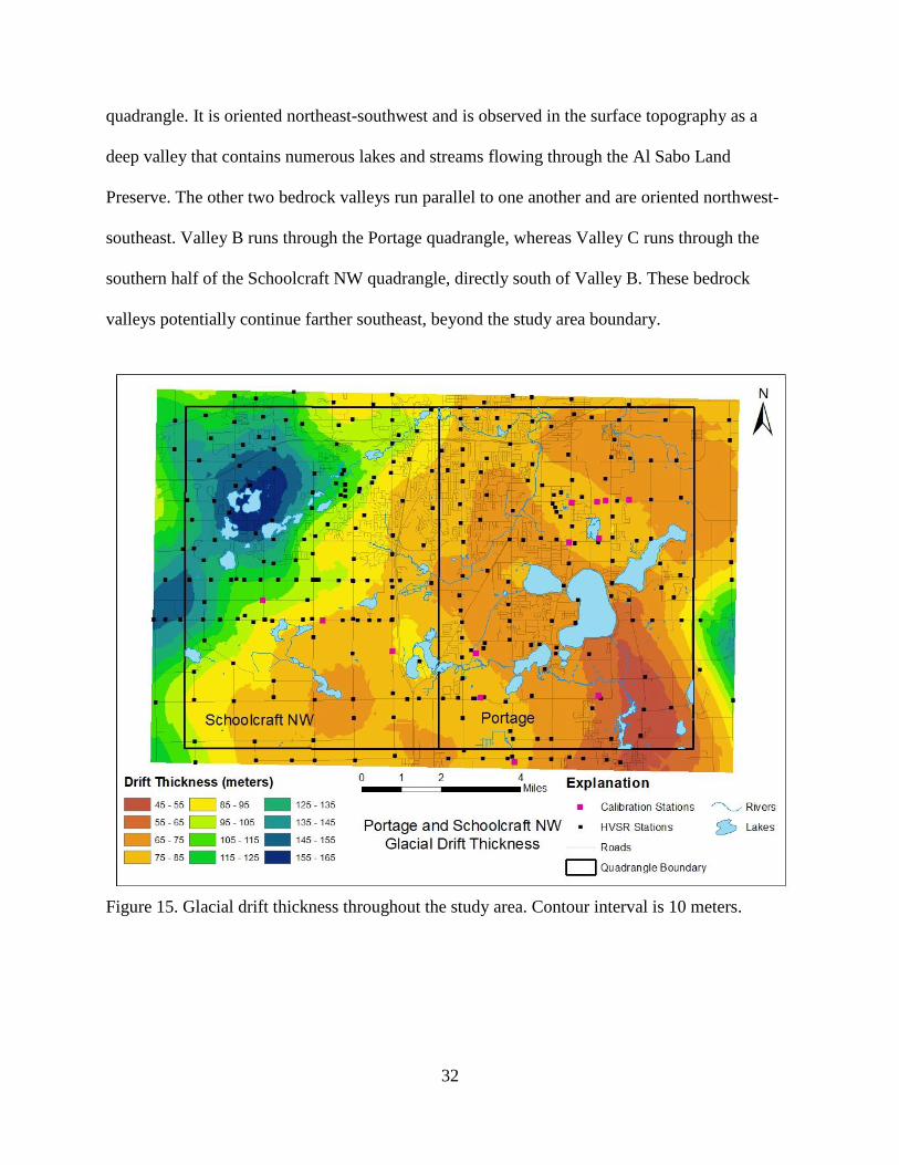
32

quadrangle. It is oriented northeast-southwest and is observed in the surface topography as a

deep valley that contains numerous lakes and streams flowing through the Al Sabo Land

Preserve. The other two bedrock valleys run parallel to one another and are oriented northwest-

southeast. Valley B runs through the Portage quadrangle, whereas Valley C runs through the

southern half of the Schoolcraft NW quadrangle, directly south of Valley B. These bedrock

valleys potentially continue farther southeast, beyond the study area boundary.

Figure 15. Glacial drift thickness throughout the study area. Contour interval is 10 meters.

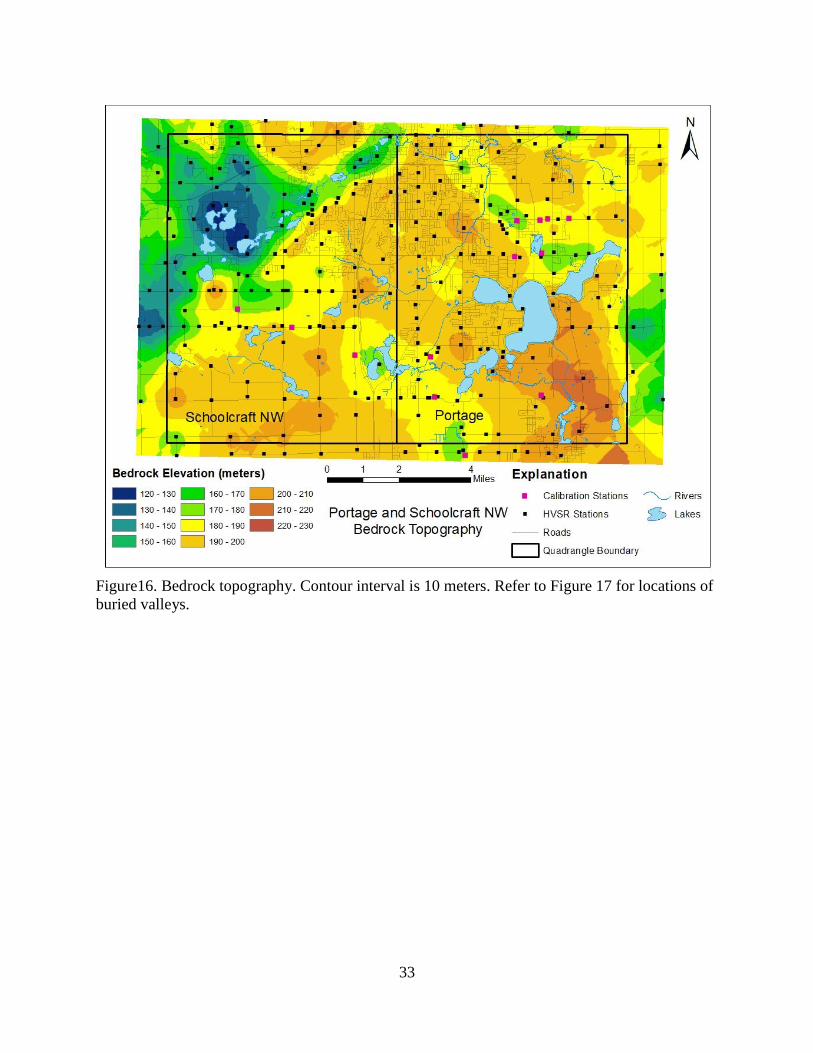
33

Figure16. Bedrock topography. Contour interval is 10 meters. Refer to Figure 17 for locations of

buried valleys.

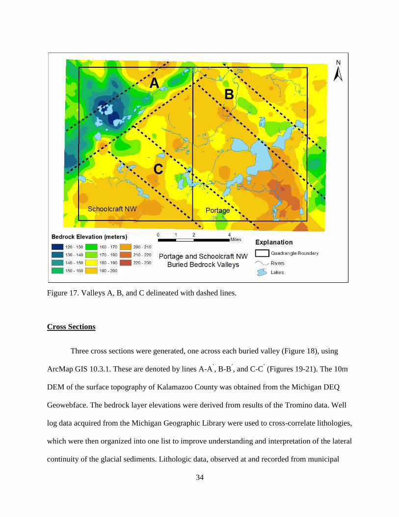
34

Figure 17. Valleys A, B, and C delineated with dashed lines.

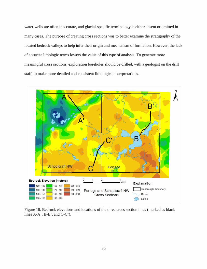
Cross Sections

Three cross sections were generated, one across each buried valley (Figure 18), using

ArcMap GIS 10.3.1. These are denoted by lines A-A’, B-B

’, and C-C

’ (Figures 19-21). The 10m

DEM of the surface topography of Kalamazoo County was obtained from the Michigan DEQ

Geowebface. The bedrock layer elevations were derived from results of the Tromino data. Well

log data acquired from the Michigan Geographic Library were used to cross-correlate lithologies,

which were then organized into one list to improve understanding and interpretation of the lateral

continuity of the glacial sediments. Lithologic data, observed at and recorded from municipal

35

water wells are often inaccurate, and glacial-specific terminology is either absent or omitted in

many cases. The purpose of creating cross sections was to better examine the stratigraphy of the

located bedrock valleys to help infer their origin and mechanism of formation. However, the lack

of accurate lithologic terms lowers the value of this type of analysis. To generate more

meaningful cross sections, exploration boreholes should be drilled, with a geologist on the drill

staff, to make more detailed and consistent lithological interpretations.

Figure 18. Bedrock elevations and locations of the three cross section lines (marked as black

lines A-A’, B-B’, and C-C’).

36

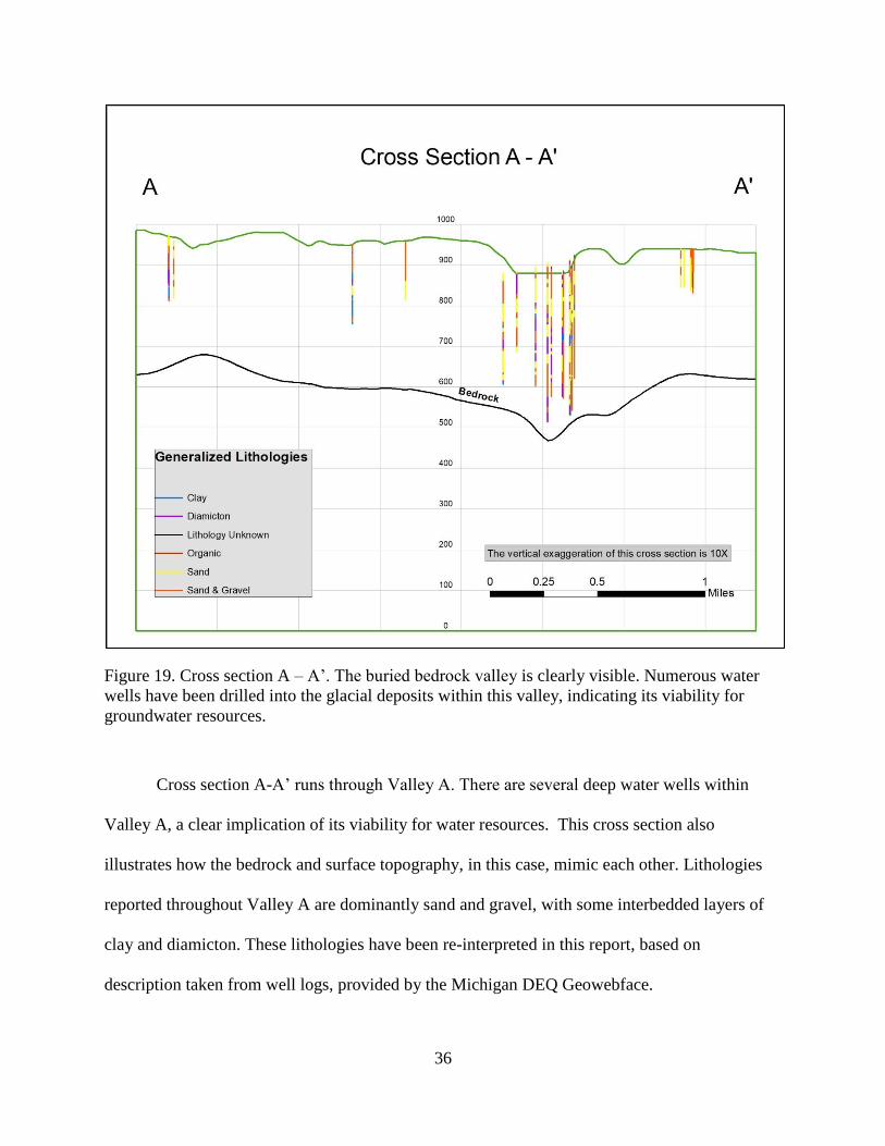
Figure 19. Cross section A – A’. The buried bedrock valley is clearly visible. Numerous water

wells have been drilled into the glacial deposits within this valley, indicating its viability for

groundwater resources.

Cross section A-A’ runs through Valley A. There are several deep water wells within

Valley A, a clear implication of its viability for water resources. This cross section also

illustrates how the bedrock and surface topography, in this case, mimic each other. Lithologies

reported throughout Valley A are dominantly sand and gravel, with some interbedded layers of

clay and diamicton. These lithologies have been re-interpreted in this report, based on

description taken from well logs, provided by the Michigan DEQ Geowebface.

37

Figure 20. Cross section B – B’. Valley B is more subdued in relief than Valley A. No wells in

this area are drilled to bedrock.

The bedrock surface in cross section B-B’ displays gentle relief. Valley B is not as clearly

incised as Valley A, showing only approximately 40 meters of relief. Cross section B-B’

illustrates the normal depths of the municipal water wells within the study area. The wells

displayed on this cross section are drilled to depths of approximaely 90 feet, and extend down

through the first impermeable clay/diamicton layer. However, there is approximately a total of

150 feet of glacial outwash lying above the bedrock surface. The deeper sections of these

outwash sediments can be futher explored and assessed for water resource viability.

38

Figure 21. Cross section C – C’. Similar to Valley B, the relief is subdued, and no wells in the

area drill to bedrock. In some areas, over 200ft of glacial outwash could still be explored.

Cross section C-C’ depicts a bedrock valley, showing gentle relief of approximately 35

meters. Also, this cross section shows that there are no wells within this area that drill deeper

than approximately 90 feet. Lithologies of these wells are primarily sand and gravel, with very

few occurrences of clay or diamicton. Several hundred feel of deeper glacial outwash has not

been drilled, and has yet to be assessed.

39

CHAPTER V

DISCUSSION

Bedrock Valleys

The objectives of this study were to (1) map the bedrock topography of the Portage and

Schoolcraft NW quadrangles, and (2) interpret and delineate any bedrock valleys located within

these quads. The HVSR method was successful in locating and delineating bedrock valleys.

Within the study area, there are three bedrock valleys, Valleys A, B, C (Refer to Figure 17).

Valley A has the sharpest relief of the three valleys, and is the only bedrock valley in the study

area to also be visible on the land surface. Valleys B and C are both perpendicular to Valley A in

the bedrock topography, and the linear arrangement of lakes and rivers in the study area.

Valley A is deeply incised into the bedrock with an overall relief of approximately 65

meters. It is located within the Schoolcraft NW quadrangle, northwest of another linear trend of

lakes and streams (Figure 22). It is possible that Valley A is a palimpsest tunnel valley, formed at

some point during the LGM. This would explain its expression on the surface topography

through a major depositional feature: the Kalamazoo Moraine. Valley A could have been eroded

during a Saginaw Lobe advance, filled with ice and debris, and then later overridden by another

advance of the Lake Michigan Lobe. Progradation of outwash from the Lake Michigan Lobe

covered the valley, and then subsided during meltout of the buried ice blocks, exhuming the

valley. This is clear on the surface DEM of the study area, which shows how the surface valley

overlaying Valley A is visible through the Kalamazoo Moraine (Figure 3). The results of this

investigation show how that surface valley is expressed in the bedrock as Valley A (Figure 22).

40

Figure 22. Bedrock and surface valleys. Note that both are parallel to each other, and the flow

direction of the Saginaw Lobe (northeast-southwest).

Valley A is possibly a tunnel valley eroded by the Saginaw Lobe of the Laurentide Ice

Sheet. Kehew et al. (2012) outlined several criteria used to identify tunnel valleys. These include

(1) orientation parallel or sub-parallel to ice flow direction, (2) long, undulating profiles that can

be convex upward (3) termination near the end of former ice margins, and (4) the presence of

other subglacial landforms in the same vicinity (such as eskers or drumlins). Valley A is parallel

to the glacial flow lines of the Saginaw Lobe during its Late Glacial Maximum advance, which

were northeast-southwest. It is also likely that Valley A extends beyond the study area both to

the northeast and the southwest, since tunnel valleys can sometimes have lengths upwards of 100

41

km (Kehew et al. 2012). Cross section A-A’ reveals both the sharpness of this relief displayed in

Valley A and the characteristics of the sediment infill (Figure 19). Large, unconsolidated

packages of coarse sand and gravel, along with interbedded layers of silt and clay are the

dominant lithologies. During ice retreat, valley sides may sometimes slump and fill in the valley.

Although these coarse-grained deposits make highly productive aquifers (due to high porosities

in glacial sediment), the heterogeneity and chaotic assemblage of the sediment makes continuity

difficult to accurately assess.

Valleys B and C are possibly remnants of the pre-glacial drainage network eroded soon

after the first glaciation that occurred after the bedrock was deposited. Rieck and Winters (1979)

attribute surface depressions containing linear chains of lakes, streams, and other waterbodies as

indicative of bedrock valleys. They propose that the surface mimics the bedrock topography.

Although Valley A is expressed on both the land surface and the bedrock, as shown by cross

section A-A’, this is not the case for all three valleys. Bedrock Valleys B and C trend

perpendicular to the surface valley containing water bodies within the quad. Therefore these

surface water bodies are not invariably expressions of bedrock topography in this case. Possibly,

it could be that the lakes in the Portage quadrangle near Valley B and Valley C are kettle lakes,

associated with ice retreat (depositional) and not associated with ice advance (erosional).

Advance of the Lake Michigan Lobe would have later buried the lowland area vacated by the

Saginaw Lobe. This advance covered the region with a broad outwash plain that gently slopes

down toward the east, emanating from the Kalamazoo Moraine directly west of the study area

(Kehew et al. 2005). Ice and debris from the Saginaw Lobe would have subsequently been

buried by this event, forming kettle lakes as the buried ice melted.

42

However, the orientation of these water bodies is perfectly aligned with Saginaw Lobe

flow direction. Furthermore, they are parallel to the lakes and streams within the surface valley

that overlies Valley A (Figure 22). Therefore, a possible explanation is that these lakes lie within

a Saginaw Lobe tunnel valley that did not incise into the bedrock, and were therefore undetected

by the Tromino.

Any tunnel valleys that do not completely incise into bedrock will be undetected by the

HVSR method, due to the absence of a strong (>2.5:1) acoustic impedance contrast. This

identifies a shortcoming of the Tromino in locating buried tunnel valleys. This is likely the case

with the surface valley containing linear chains of lakes and streams that are not expressed in the

bedrock. This result is also contrary to previous hypothesis on the origin of those lakes. Kehew et

al. (1999) proposed that the linear trend of lakes within the Portage quadrangle were the surface

expression of an incised tunnel valley, related to the Saginaw Lobe. While it is still possible that

these lakes lie within a tunnel valley, the results of this investigation show that there is no incised

bedrock valley within the Portage quadrangle. Instead, two bedrock valleys with gentle, subdued

relief flow perpendicular to Saginaw Lobe flow direction, 90 degrees from the orientation of the

northeast-southwest trend of lakes (Figure 17).

There is great potential for water resources within the Schoolcraft NW and Portage

quadrangles. Several tens of meters (40 - 50) of unconsolidated glacial sediment lay within these

valleys, far below the depths of most current municipal water wells (~90 ft). Further exploration

of these areas could prove successful in finding aquifers that are capped by clay and diamicton

layers that were deposited during advances of the LIS. If future exploration boreholes were

drilled throughout these subsurface bedrock valleys, the impermeable clay and diamicton layers

could be cross-correlated, and porous zones of sand and gravel could be identified.

43

Quality of the HVSR Data

The HVSR method was useful for determining sediment thickness and bedrock

topography. Calculated depths to bedrock deviated less than 10% from known depths at the

calibration wells, when applying the calibration curve derived from this study (Table 1). One

focus of this study was to identify buried bedrock valleys. The HVSR method revealed three

such valleys, one of which is interpreted to be a glacial tunnel valley. This interpretation is based

on the relief of Valleys B and C, which is approximately 10 to 15 meters extending for an

average width of 0.5 – 1.5 miles. However, Valley A has a sharper relief of 30 to more than 50

meters in some areas.

Table 1. Calibration curve HVSR data

Station

ID Well ID fo

Bedrock Depth

(m)

Calculated Depth

(m)

Vs

ft/sec

%

Error

KAL-271 KAL-03-03 1.5 52 56.08 1026.00 7.59

KAL-269 KAL-03-01 1.38 57 63.33 1032.24 11.12

KAL-354 Pfizer MW-121 1.47 68 57.75 1311.24 15.03

KAL-156 KAL-03-04 1.25 69 73.18 1135.00 5.76

KAL-154 KAL-03-02 1.19 79 78.63 1232.84 0.40

KAL-310 11696 1.19 83 78.63 1289.96 4.81

KAL-337 Pfizer MW-156 1.06 85 93.09 1187.20 9.08

KAL-335 Pfizer MW-157 1.03 87 97.08 1178.32 11.36

KAL-339 Pfizer MW-106 0.94 107 110.94 1319.76 3.70

KAL-430 11621 0.94 121 110.94 1492.72 8.32

KAL-08 5975 1.13 95 84.80 1414.76 11.12

KAL-402 6899 1.03 91 97.08 1236.00 6.17

Kal-405 18817 1.03 108 97.08 1238.00 10.03

The values calculated for a and b for the power law equation were 101.36 and -1.46 using

the local calibration curve. These values can be compared with other previous HVSR studies,

both in Michigan and other locations. Chandler and Lively (2014) derived a local calibration

44

curve within the Twin Cities metro area with a = 83 and b = -1.232. John Esch of the Michigan

Department of Environmental Quality office of Oil, Gas and Minerals (pers communication

2017) derived a local calibration curve for south-central Michigan with power law values a =

68.716 and b = -1.224. An earlier example of use of the power law equation comes from Seht

and Wohlenberg (1999) who mapped the Rhine graben in Germany use the HVSR method

jointly with a seismic reflection survey. For their study, they derived a = 96 and b = -1.388.

The HVSR method has also been used in southwest Michigan by other graduate students

at Western Michigan University. Scott Feldpausch (2017) mapped the Maple Gove and Dowling

7.5’ quadrangles and derived a = 121.09 and b = -1.188. Karl Backhaus (2018) mapped the

Bronson North and Bronson South 7.5’ quadrangles using the HVSR method and derived a =

80.492 and b = -1.869.

There are several explanations for the differences in these values from the local equation

derived for this study: (1) different local geology for each study area, (2) different recording

lengths at each calibration well, (3) different numbers of calibration wells, and (4) varying depths

at each calibration well. For example, Feldpausch (2017) utilized 21 calibration wells, and

Backhaus (2018) used 11 calibration wells. Generally, the greater number of calibration points,

the more improved the accuracy of the local calibration curve.

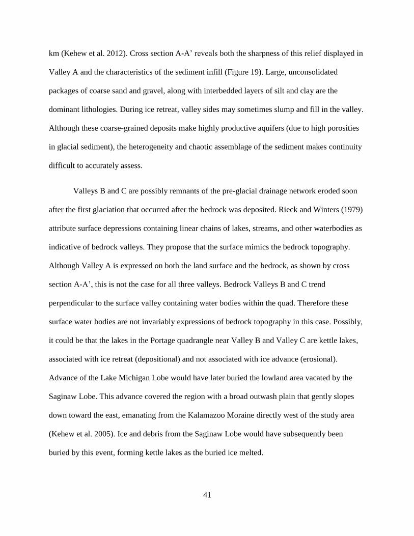
Weather is an important factor to consider when collecting HVSR data. Low-frequency

microtremors can be caused by ocean waves, distant earthquakes, wind, and other meteorological

sources (Bonnefoy-Claudet et al. 2006). On windy days, the resonance frequency was commonly

obliterated by low-frequency noise, such as station KAL-172 (Figure 23). Therefore, care was

taken to collect on days with gentle wind, in order to ensure the resonance peak could be

45

identified, and not be obliterated by low-frequency noise. This factor should be considered for

any future HVSR studies.

Figure 23. Station KAL-172. The resonance frequency is not apparent; however, there is a clear

peak at a much higher frequency. This is indicative of a boundary at 6-7 ft, such as diamicton, or

a local or industrial noise source. The large disturbance within the lower frequency spectra (<1.0

Hz) is likely due to wind.

HVSR Sources of Error

Resonance frequency of the subsurface depends on how much ambient seismic noise is

present within the subsurface. Resonance implies a dominant, although not consistent, frequency.

Therefore, based on processing data from the Tromino, it is likely that the resonance frequency

varies about a mean value with a standard deviation. I took 10 duplicate recordings, each in the

same location, on the Western Michigan west campus in front of Wood Hall (Table 2). Another

10 duplicate recordings were also taken in the parking lot at the Al Sabo land preserve (Table 3).

These recordings were processed and analyzed to assess the fluctuation of resonance frequency

with each recording. Furthermore, one single three-hour recording was taken to assess the

46

variability of ambient noise during a long period. This recording was parsed into overlapping 30

min segments to show the overall change of resonance frequency over time (Table 4).

47

Table 2. Al Sabo Land Preserve error recordings

Station

ID

Elevation

(ft) Latitude Longitude

Rec.Time

(min)

Pr.Window

(sec) Freq0 Std.Dev. SESAME Z (m)

Test-1 948 42.21217 -85.674 18 20 1.09 0.09 8 89

Test-2 948 42.21217 -85.674 18 20 1.09 0.04 9 89

Test-3 948 42.21217 -85.674 18 20 1.03 0.03 9 96

Test-4 948 42.21217 -85.674 18 20 1.13 0.03 9 84

Test-5 948 42.21217 -85.674 18 16 1.13 0.05 9 84

Test-6 948 42.21217 -85.674 18 20 1.13 0.04 9 84

Test-7 948 42.21217 -85.674 18 20 0.94 0.05 9 109

Test-8 948 42.21217 -85.674 18 20 1.19 0.05 9 78

Test-9 948 42.21217 -85.674 18 20 1.09 0.05 9 89

Test-10 948 42.21217 -85.674 18 20 1.03 0.09 8 96

48

Table 3. Wood Hall error recordings

Station

ID

Elevation

(ft) Latitude Longitude

Rec.Time

(min)

Pr.Window

(sec) Freq0 Std.Dev. SESAME Z (m)

WMU-1 921 42.28275 -85.617 18 20 1.13 0.03 9 84

WMU-2 921 42.28275 -85.617 18 20 1.13 0.03 9 84

WMU-3 921 42.28275 -85.617 18 20 1.13 0.04 9 84

WMU-4 921 42.28275 -85.617 18 20 0.97 0.03 9 104

WMU-5 921 42.28275 -85.617 18 20 1.03 0.08 8 96

WMU-6 921 42.28275 -85.617 18 20 1.06 0.12 7 92

WMU-7 921 42.28275 -85.617 18 20 1.09 0.06 8 89

WMU-8 921 42.28275 -85.617 18 20 1.06 0.06 8 92

WMU-9 921 42.28275 -85.617 18 20 1.03 0.01 9 96

WMU-10 921 42.28275 -85.617 18 20 0.94 0.03 9 109

49

Table 3. Three-hour recording

Window (min) Latitude Longitude f0 St Dev SESAME Z(m)

0-30 43.10018 -85.60416 1.41 0.11 8 61.38

20-50 43.10018 -85.60416 1.19 0.26 7 78.63

40-70 43.10018 -85.60416 1.25 0.17 7 73.18

60-90 43.10018 -85.60416 1.25 0.01 9 73.18

80-110 43.10018 -85.60416 1.25 0.06 9 73.18

100-130 43.10018 -85.60416 1.19 0.13 7 78.63

120-150 43.10018 -85.60416 1.25 0.01 9 73.18

140-170 43.10018 -85.60416 1.25 0.12 8 73.18

160-180 43.10018 -85.60416 1.25 0.11 8 73.18

50

Fluctuation in resonance frequency peaks demonstrates the variability of seismic noise in

a given location. The presence or absence of seismic noise leads to different peak forms, such as

sharp, plateau, or multiple peaks. This error investigation outlines several obstacles in front of

generating a power law function. There must be a statistically significant number of calibration

wells within the survey area to account for any variability in bedrock elevation, and more than

one recording should be taken at each calibration station. Furthermore, recordings at these

calibration wells should be greater than the sampling time for other HVSR stations in order to

reduce the standard deviation of the H/V ratio. Outliers on the calibration curve could be due to a

number of factors, such as faulty well depth data, bad weather, or poor instrumental coupling.

These should be eliminated, or re-sampled to ensure the validity of the calibration curve.

The standard deviation range for each HVSR point defines an uncertainty range for the

depth calculated at that location. Tunnel valley depths can vary greatly, along with the character

of the substrate, the hydrologic system, and the compaction of the sediment filling the valley.

Therefore, the standard deviation should also be expected to vary in accordance with the valley

with which it is associated.

51

CHAPTER IV

CONCLUSIONS

The HVSR method was successfully used to map the bedrock topography of the Portage

and Schoolcraft NW quadrangles. Three buried valleys were identified, one of which is

interpreted to be a glacial tunnel valley because of its orientation parallel to the flow direction of

the Saginaw Lobe, sharp relief along the valley sides, long extent, and surface expression

associated with topographic lows and a linear arrangement of lakes and streams. Numerous other

explanations exist for the two other valleys located in the study area, such as: (1) remnants of a

pre-glacial drainage network, or (2) valleys from a pre-Wisconsinan advance. The surface valley

containing the linear trend of lakes was not incised into the bedrock. These lakes could instead

be the surface expression of a tunnel valley that did not incise into the bedrock.

Cross section analysis revealed several hundreds of feet of drift in the bedrock valleys,

which can be further delineated and examined in order to assess water resource viability. This

demonstrates the usefulness of the HVSR method in determining sediment thickness, the results

of which can be applied to map bedrock topography, sediment thicknesses, and potential aquifer

occurrence.

Results of the HVSR survey were within 10% of known values of bedrock depth at the

calibration stations; however, additional calibration stations would be useful to help improve the

accuracy of this type of surveying.

Glacial drift is largely heterogeneous and can be laterally and vertically variable.

Furthermore, the presence of several feet of clay or diamicton can produce secondary resonance

52

frequency peaks that can be misinterpreted for the bedrock depth. Weather can also influence

resonance frequency. Heavy winds and poor coupling can lead to incoherent results, causing

noise to obliterate the signal at the peak frequency.

However, the HVSR method is effective provided there is a strong acoustic impedance

contrast between the bedrock and overlaying sediment. Clear resonance frequency peaks were

not observed in all locations in the study area. This could be due to the soft, weathered surfaces

of the Mississippian-age Coldwater Shale bedrock which would lower the acoustic impedance

contrast. This could also be due to the presence of tills or diamicton, an overriding

monochromatic noise source, or poor instrument coupling.

53

REFERENCES

Altuhafi, F., B. A. Baudet, and P. Sammonds. 2010. The mechanics of subglacial sediment: an

example of new “transitional” behaviour. Canadian Geotechnical Journal 47:775–790.

Backhaus, K. J. 2018. Geologic Mapping of the Bronson North and Bronson South 7.5-Minute

Quadrangles, Branch County, Michigan. Unpublished Masters thesis.

Benn, D. I. and D. J. A. Evans. 2010. Glaciers and Glaciation. Second edition. 802 p. Hobber

Education, London. ISBN 978-0-340-905791

Boulton, G. S., K. E. Dobbie, and S. Zatsepin. 2001. Sediment deformation beneath glaciers and

its coupling to the subglacial hydraulic system. Quaternary International 86:3–28.

Boulton, G. S. and R. C. A. Hindmarsh. 1987. Sediment deformation beneath glaciers: Rheology

and geological consequences. Journal of Geophysical Research: Solid Earth 92:9059-9082

Brennand, T. A. and J. Shaw. 1994. Tunnel channels and associated landforms, south-central

Ontario: their implications for ice-sheet hydrology. Canadian Journal of Earth Sciences

31:505-522

Chandler V. W. and R. S. Lively. 2014. Evaluation of the Horizontal-to-Vertical Spectral Ratio

(HVSR) passive seismic method for estimating the thickness of Quaternary deposits in

Minnesota and adjacent parts of Wisconsin. Minnesota Geological Survey Open File Report

14-01. 54p.

Cofaigh, C. (1999). Tunnel valley genesis. Progress in Physical Geography 20, 1:1-19

Cutler, P. M., P. M. Colgan, and D. M. Mickelson. 2002. Sedimentologic evidence for outburst

floods from the Laurentide Ice Sheet margin in Wisconsin, USA: implications for tunnel-

channel formation. Quaternary International 90:23–40.

Feldpausch, S. 2017. Gravity and passive seismic methods used jointly for understanding the

subsurface in a glaciated terrain: Dowling and Maple Grove quadrangles, Barry County,

Michigan. Unpublished masters thesis.

Fisher, T. G., H. M. Jol, A. M. Boudreau. 2005. Saginaw Lobe tunnel channels (Laurentide Ice

Sheet) and their significance in south-central Michigan, USA. Quaternary Science Reviews

24:2375-2391

Gao, C. 2011. Buried bedrock valleys and glacial and subglacial meltwater erosion in southern

Ontario, Canada. Canadian Journal of Earth Sciences 48:801–818.

Gosar, A., and A. Lenart. 2009. Mapping the thickness of sediments in the Ljubljana Moor basin

(Slovenia) using microtremors. Bulletin of Earthquake Engineering 8:501–518.

Guillier, B., K. Atakan, J. Chatelain, et al. 2008. Influence of instruments on the H/V spectral

ratios of ambient vibrations. Bulletin of Earthquake Engineering 6: 3.

Haefner, R. J., Sheets, R. A., Andrews, R. E. Evaluation of the Horizontal-to-Vertical Spectral

54

Ratio (HVSR) Seismic Method to Determine Sediment Thickness in the Vicinity of the

South Well Field, Franklin County, OH. Ohio Journal of Science 110, 4:77-85.

Hooke, R. L., and C. E. Jennings. 2006. On the formation of the tunnel valleys of the southern

Laurentide ice sheet. Quaternary Science Reviews 25:1364–1372.

Huuse, M., and H. Lykke-Andersen. 2000. Overdeepened Quaternary valleys in the eastern

Danish North Sea: morphology and origin. Quaternary Science Reviews 19:1233–1253.

Johnson, C. D. and J. W. Lane Jr. 2016. Statistical comparison of methods for estimating

sediment thickness from horizontal-to-vertical spectral ratio (HVSR) seismic methods: an

example from Tylerville, Connecticut, USA. Symposium on the Application of Geophysics

to Engineering and Environmental Problems, Marth 20-24, 2016, Denver, Colorado,

Proceedings: Denver, Colorado, Environmental and Engineering Geophysical Society. 7p.

Jørgensen, F., and P. B. E. Sandersen. 2006. Buried and open tunnel valleys in Denmark—

erosion beneath multiple ice sheets. Quaternary Science Reviews 25:1339–1363.

Kehew, A. 2012. Subglacial drainage of the Saginaw Lobe, Michigan, USA. Quaternary

International 279.

Kehew, A. E., S. P. Beukema, B. C. Bird, and A. L. Kozlowski. 2005. Fast flow of the Lake

Michigan Lobe: evidence from sediment-landform assemblages in southwestern Michigan,

USA. Quaternary Science Reviews 24:2335–2353.

Kehew, A. E., J. Esch, S. Karki. 2017. Sediment-landform assemblages in southern Michigan:

Implications for basal processes of the Saginaw Lobe of the Laurentide ice sheet. The

Geological Society of America Special Paper 530:115-137

Kehew, A. E., J. M. Esch, A. L. Kozlowski, and S. K. Ewald. 2012a. Glacial landsystems and

dynamics of the Saginaw Lobe of the Laurentide Ice Sheet, Michigan, USA. Quaternary

International 260:21–31.

Kehew, A. E., S. K. Ewald, J. M. Esch, and A. L. Kozlowski. 2013. On the origin of tunnel

valleys of the Saginaw Lobe of the Laurentide Ice Sheet; Michigan, USA. Boreas 42:442–

462.

Kehew, A. E., Nicks, L. P., & Straw, W. T. (1999). Palimpsest tunnel valleys: Evidence for

relative timing of advances in an interlobate area of the Laurentide ice sheet. Annals of

Glaciology 28:47-52

Kehew, A. E., J. A. Piotrowski, and F. Jørgensen. 2012. Tunnel valleys: Concepts and

controversies — A review. Earth-Science Reviews 113:33–58.

Kozlowski, A. L., A. E. Kehew, B.C. Bird. 2005. Outburst flood origin of the Central Kalamazoo

River Valley, Michigan, USA. Quaternary Science Reviews 24:2354-2374

Lane, J. W., E. A. White, G. V Steele, and J. C. Cannia. 2008. Estimation of bedrock depth using

the horizontal-to-vertical (H/V) ambient-noise seismic method. Symposium on the

Application of Geophysics to Engineering and Environmental Problems, April 6-10, 2008,

55

Philadelphia, Pennsylvania, Proceedings: Denver, Colorado, Environmental and

Engineering Geophysical Society:1–13.

Lang, N., and E. W. Wolff. 2011. Interglacial and glacial variability from the last 800 ka in

marine, ice and terrestrial archives. Clim. Past 7:361–380.

Leverett, F., and Taylor, F. B., 1915. The Pleistocene of Indiana and Michigan and the History of

the Great Lakes: U.S. Geological Survey Monograph 53

Michigan Department of Environmental Quality, Office of Oil, Gas, and Minerals.

http://www.deq.state.mi.us/GeoWebFace/

Michigan Geographic Data Library - MiGDL Center for Geographic Information.

https://www.mcgi.state.mi.us/mgdl/

Monaghan, G.W., Larson, G.J., Gephart, G.D., 1986. Late Wisconsinan drift stratigraphy of the

Lake Michigan Lobe in southwestern Michigan. Geological Society of America Bulletin

97:329–443

Nakamura, Y. 1989. A Method for Dynamic Characteristics Estimation of Subsurface using

Microtremor on the Ground Surface. Quarterly report of RTRI 30:25-33

Reick, R. L., Winters, H. A. 1979. Annals of the Association of American Geographers 69,

2:276-288.

Seht, M. I. V, and J. Wohlenberg. 1999. Microtremor Measurements Used to Map Thickness of

Soft Sediments. Bulletin of the Seismological Society of America 89:250–259.

SESAME, 2004, Guidelines for the implementation of the H/V spectral ratio technique on

ambient vibrations. Measurements, processing and interpretation, WP12 European

commission - Research general directorate project no. EVG1-CT-2000-0026 SESAME,

report D23.12, 62 pp.

Shaw, J. 2010. In defense of the meltwater (megaflood) hypothesis for the formation of

subglacial bedform fields. Journal of Quaternary Science 25:249-260

Shaw, J., D. R. Kvill, R. B. Rains. 1989. Drumlins and catastrophic subglacial sheetfloods.

Sedimentary Geology 62:177-202

56

APPENDIX A

HVSR Data

57

Data by Benjamin Seiderman. Kalamazoo County, MI

Local Eq. 11/2/2017 HVSR with Tromino as of 11/2/2017 Station

No.

Lat -Deg

N

Long-Deg

W UTM-mN UTM-mE

Elev

(m) F0

Std.

Dev.

Max

Ampl SESAME

Thicknes

s (m)

Bedrock

Elevation (m)

KAL-

150 42.16360 -85.60255 4668886.3 615437.8 266.7 1.13 9.7 3.74 7 85.09 181.61

KAL-

151 42.16156 -85.60309 4668659.1 615397.1 266.7 1.13 0.07 4.34 8 85.09 181.61

KAL-

152 42.14336 -85.60806 4666631.5 615019.4 267.0 1.09 0.1 4.3 8 89.62 177.39

KAL-

153 42.14334 -85.60733 4666630.1 615079.6 267.0 1.09 0.09 4.56 8 89.62 177.39

KAL-

154 42.14370 -85.60442 4666674.2 615319.7 267.0 1.19 0.06 5.02 8 78.99 188.02

KAL-

155 42.14324 -85.54545 4666704.4 620192.8 264.3 1.44 0.18 3.21 6 60.05 204.22

KAL-

156 42.21592 -85.53145 4674794.9 621211.3 261.2 1.25 0.02 2.5 9 73.60 187.62

KAL-

157 42.14368 -85.60261 4666674.1 615469.2 266.4 1.16 0.02 6.61 9 81.94 184.45

KAL-

158 42.14204 -85.59219 4666506.3 616333.3 264.6 1.19 0.04 4.74 9 78.99 185.58

KAL-

159 42.14435 -85.57930 4666780.1 617393.9 266.4 1.25 0.01 5.27 9 73.60 192.80

KAL-

160 42.14340 -85.61542 4666626.3 614411.3 266.4 1.13 0.06 4.2 9 85.09 181.31

KAL-

161 42.14330 -85.62306 4666604.3 613779.6 267.0 1.19 0.09 4.84 8 78.99 188.02

KAL-

162 42.14316 -85.63490 4666573.2 612801.5 270.7 1.19 0.05 6.28 9 78.99 191.67

KAL-

163 42.14510 -85.64746 4666772.8 611760.4 267.9 1.16 0.15 6.4 7 81.94 185.98

KAL-

164 42.14296 -85.64046 4666544.4 612342.4 270.1 1.16 0.1 5.79 8 81.94 188.11

KAL- 42.13621 -85.61326 4665830.5 614602.4 265.8 1.25 0.05 4.02 9 73.60 192.19

58

165

KAL-

166 42.12426 -85.61280 4664504.6 614661.7 269.4 1.13 0.23 4.4 6 85.09 184.35

KAL-

167 42.12134 -85.62046 4664169.7 614034.2 267.3 1.41 0.31 6.11 7 61.89 205.42

KAL-

168 42.12132 -85.60338 4664190.7 615446.1 264.9 1.16 0.17 3.45 7 81.94 182.93

KAL-

169 42.12131 -85.59113 4664206.6 616458.4 266.1 1 0.18 5.62 5 101.44 164.65

KAL-

170 42.12204 -85.58895 4664290.0 616637.5 266.4 0.94 0.02 5.47 8 110.88 155.52

KAL-

171 42.13137 -85.58978 4665324.9 616552.1 263.3 1.06 0.09 5.67 8 93.29 170.06

KAL-

172 42.14333 -85.56798 4666682.8 618331.1 265.8 0.16 0.03 15.46 4 1414.77 -1148.98

KAL-

173 42.15457 -85.56944 4667928.8 618190.1 262.1 3.94 0.33 7.27 7 14.12 248.01

KAL-

174 42.12130 -85.58011 4664220.4 617369.8 263.7 1.47 0.22 4.55 7 58.29 205.36

KAL-

175 42.12122 -85.56969 4664226.1 618231.0 263.7 1.19 0.04 6.24 9 78.99 184.66

KAL-

176 42.12179 -85.56087 4664301.4 618959.2 263.3 1.34 0.15 6.89 7 66.59 196.75

KAL-

177 42.12138 -85.55391 4664265.0 619535.1 259.4 1.59 1.01 4.89 7 52.07 207.31

KAL-

178 42.12100 -85.54256 4664238.9 620473.8 262.7 1.56 0.13 5.41 8 53.52 209.22

KAL-

179 42.11982 -85.53580 4664118.0 621035.6 260.6 1.44 0.12 5.78 8 60.05 200.56

KAL-

180 42.11982 -85.53580 4664118.0 621035.6 261.8 2.34 0.92 3.84 6 29.87 231.95

KAL-

181 42.13923 -85.52417 4666289.7 621959.1 264.6 1.41 0.3 3.21 7 61.89 202.68

KAL-

183 42.12852 -85.58852 4665010.1 616660.7 265.2 1.25 0.06 5.06 9 73.60 191.58

59

KAL-

184 42.12850 -85.57642 4665024.4 617661.6 263.0 1.09 0.2 6.46 7 89.62 173.43

KAL-

185 42.12861 -85.56959 4665046.4 618225.9 262.7 1.5 0.09 7.33 8 56.62 206.12

KAL-

187 42.13967 -85.54955 4666302.2 619860.9 264.9 1.13 2.73 2.91 7 85.09 179.78

KAL-

190 42.15066 -85.61336 4667434.4 614568.4 263.7 1.19 0.07 4.1 8 78.99 184.66

KAL-

191 42.15824 -85.61361 4668276.5 614533.9 268.2 1.25 0.07 3.48 8 73.60 194.63

KAL-

192 42.16553 -85.61364 4669085.7 614518.2 270.1 1.22 0.13 3.93 7 76.21 193.84

KAL-

193 42.17113 -85.61356 4669707.5 614514.9 269.7 1.28 0.03 4.39 9 71.13 198.62

KAL-

194 42.17539 -85.61431 4670179.3 614445.1 268.5 1.31 0.14 3.76 7 68.80 199.73

KAL-

195 42.18096 -85.61489 4670797.0 614386.7 262.7 1.22 0.21 5.35 7 76.21 186.53

KAL-

196 42.18812 -85.61340 4671593.9 614497.4 259.7 1.44 0.18 5.26 7 60.05 199.64

KAL-

197 42.20045 -85.61316 4672963.3 614495.0 264.3 1.25 0.01 5.54 9 73.60 190.67

KAL-

198 42.20741 -85.61436 4673734.6 614382.8 269.7 1.19 0.04 6.14 9 78.99 190.76

KAL-

199 42.21425 -85.61462 4674493.9 614349.0 270.7 1.19 0.02 5.32 9 78.99 191.67

KAL-

200 42.22275 -85.61342 4675439.5 614433.4 274.3 1.22 0.05 5.88 9 76.21 198.11

KAL-

201 42.22865 -85.61356 4676094.8 614410.5 277.4 1.22 0.15 4.67 7 76.21 201.16

KAL-

202 42.23436 -85.61338 4676728.5 614415.7 279.2 1.19 0.09 5.2 8 78.99 200.21

KAL-

203 42.24176 -85.61450 4677548.5 614309.2 272.2 1.19 0.01 5.95 9 78.99 193.20

KAL-

204 42.24543 -85.61460 4677956.6 614295.0 279.2 1.25 0.12 5.19 8 73.60 205.60

60

KAL-

205 42.24560 -85.60631 4677985.8 614978.0 265.8 1.25 0.1 6.27 8 73.60 192.19

KAL-

206 42.24581 -85.59657 4678022.4 615781.6 272.5 1.25 0.03 6.37 9 73.60 198.90

KAL-

207 42.24278 -85.59021 4677694.6 616311.4 260.0 1.19 0.08 4.06 8 78.99 181.01

KAL-

208 42.23617 -85.58991 4676961.2 616348.5 263.0 1.05 0.05 3.18 9 94.57 168.48

KAL-

209 42.23093 -85.60162 4676363.4 615392.2 276.1 1.22 0.05 5.45 9 76.21 199.94

KAL-

210 42.22896 -85.57898 4676175.9 617263.9 261.5 1.16 0.17 4.44 7 81.94 179.57

KAL-

211 42.20152 -85.59036 4673113.6 616375.0 265.8 1.16 0.13 4.55 7 81.94 183.84

KAL-

212 42.20124 -85.58344 4673091.6 616947.0 271.9 1.34 0.1 4.64 8 66.59 205.29

KAL-

213 42.20194 -85.57493 4673180.6 617648.5 268.2 1.22 0.05 5.18 9 76.21 192.01

KAL-

214 42.20157 -85.56723 4673150.5 618284.2 263.0 1.19 0.1 5.87 8 78.99 184.05

KAL-

215 42.20001 -85.55818 4672990.0 619035.0 263.3 1.34 0.08 5.47 8 66.59 196.75

KAL-

216 42.20033 -85.54659 4673042.5 619990.9 264.6 1.22 0.03 5.41 9 76.21 188.36

KAL-

217 42.20218 -85.53978 4673256.6 620549.4 264.0 0.97 0.12 6.2 8 105.98 157.98

KAL-

218 42.20993 -85.53981 4674117.7 620532.1 265.2 1.38 0.2 6.07 7 63.84 201.34

KAL-

219 42.22867 -85.58865 4676130.4 616466.8 268.5 1.16 0.06 5.17 9 81.94 186.59

KAL-

220 42.22282 -85.58152 4675490.9 617065.7 261.2 1.44 0.23 5.84 7 60.05 201.17

KAL-

221 42.21184 -85.58865 4674261.2 616497.3 263.3 1.78 0.14 6.65 8 44.27 219.08

KAL-

222 42.20635 -85.55964 4673692.1 618902.5 269.1 1.16 0.04 6.06 9 81.94 187.19

61

KAL-

223 42.21693 -85.55477 4674873.3 619284.1 265.5 1.19 0.11 6.22 8 78.99 186.49

KAL-

224 42.22313 -85.55970 4675555.3 618865.9 268.8 1.34 0.09 4.44 8 66.59 202.24

KAL-

225 42.23249 -85.56152 4676592.4 618698.3 267.0 1.25 0.21 4.83 7 73.60 193.41

KAL-

226 42.18993 -85.60132 4671811.5 615491.5 265.2 1.16 0.18 5.14 7 81.94 183.23

KAL-

227 42.18589 -85.59097 4671377.1 616353.1 263.3 1.25 0.14 5.86 7 73.60 189.75

KAL-

228 42.17760 -85.59102 4670456.5 616364.4 264.3 1.25 0.01 5.3 9 73.60 190.67

KAL-

229 42.17163 -85.59022 4669794.2 616441.7 266.7 1.25 0.05 5.34 9 73.60 193.11

KAL-

230 42.16477 -85.59039 4669032.8 616440.4 271.0 1.75 0.22 2.54 7 45.36 225.60

KAL-

231 42.19271 -85.56123 4672175.4 618796.6 263.3 1.25 0.14 6.14 7 73.60 189.75

KAL-

232 42.18453 -85.56377 4671263.3 618602.0 263.0 1.25 0.1 6.57 8 73.60 189.45

KAL-

233 42.18453 -85.56377 4671263.3 618602.0 267.0 1.25 0.15 5.12 7 73.60 193.41

KAL-

234 42.17934 -85.55653 4670697.4 619209.4 260.6 1.25 0.02 5.91 9 73.60 187.01

KAL-

235 42.17085 -85.55784 4669752.9 619117.5 270.7 1.25 0.04 4.59 9 73.60 197.07

KAL-

236 42.16197 -85.56714 4668753.4 618366.1 269.1 1.22 0.2 6.82 7 76.21 192.93

KAL-

237 42.19355 -85.53979 4672298.7 620564.9 264.9 1.09 0.04 5.29 9 89.62 175.26

KAL-

238 42.18557 -85.53984 4671413.1 620576.3 263.0 1.38 0.24 5.27 7 63.84 199.21

KAL-

239 42.17943 -85.53148 4670742.2 621278.5 265.2 1.44 0.13 4.9 7 60.05 205.13

KAL-

240 42.18072 -85.54043 4670872.9 620536.9 267.0 1.47 0.02 3.74 9 58.29 208.71

62

KAL-

241 42.24465 -85.57904 4677918.3 617229.8 257.6 1.31 0.06 3.96 9 68.80 188.76

KAL-

242 42.24280 -85.56988 4677724.9 617988.9 264.6 1.34 0.11 3.11 8 66.59 197.97

KAL-

243 42.24721 -85.55856 4678230.8 618914.4 263.3 1.25 0.04 5 9 73.60 189.75

KAL-

244 42.24596 -85.55000 4678104.0 619622.9 262.1 1.22 0.08 5.22 8 76.21 185.92

KAL-

245 42.24519 -85.53653 4678037.3 620736.4 259.7 1.34 0.1 5.5 8 66.59 193.10

KAL-

246 42.24520 -85.51377 4678071.0 622613.9 261.8 1.31 0.06 4.84 9 68.80 193.03

KAL-

247 42.24519 -85.51377 4678069.3 622613.6 262.4 1.47 0.03 5.04 9 58.29 204.14

KAL-

248 42.23799 -85.53884 4677234.8 620558.8 259.7 1.47 0.03 6.42 9 58.29 201.40

KAL-

249 42.23155 -85.54017 4676518.1 620461.8 262.1 1.47 0.1 4.93 8 58.29 203.84

KAL-

250 42.22359 -85.54321 4675629.0 620226.0 261.8 1.25 0.03 5.51 9 73.60 188.23

KAL-

251 42.21560 -85.53742 4674750.5 620718.8 264.9 1.19 0.29 4.13 7 78.99 185.88

KAL-

252 42.21604 -85.52062 4674823.1 622105.1 264.6 1.25 0.17 5.53 6 73.60 190.97

KAL-

253 42.21675 -85.50583 4674922.9 623323.9 264.0 1.5 0.03 4.48 9 56.62 207.33

KAL-

254 42.25423 -85.64804 4678888.4 611520.6 289.0 1.16 0.11 3.76 8 81.94 207.06

KAL-

255 42.24515 -85.64802 4677880.9 611538.2 280.0 1.19 0.02 4.24 9 78.99 201.01

KAL-

256 42.23949 -85.64476 4677256.6 611816.6 279.0 0.78 0.06 5.51 8 145.00 134.00

KAL-

257 42.23648 -85.64821 4676917.9 611537.8 268.0 0.88 0.08 4.2 8 121.91 146.09

KAL-

258 42.22989 -85.64738 4676187.4 611617.8 284.0 1.06 0.05 4.53 9 93.29 190.71

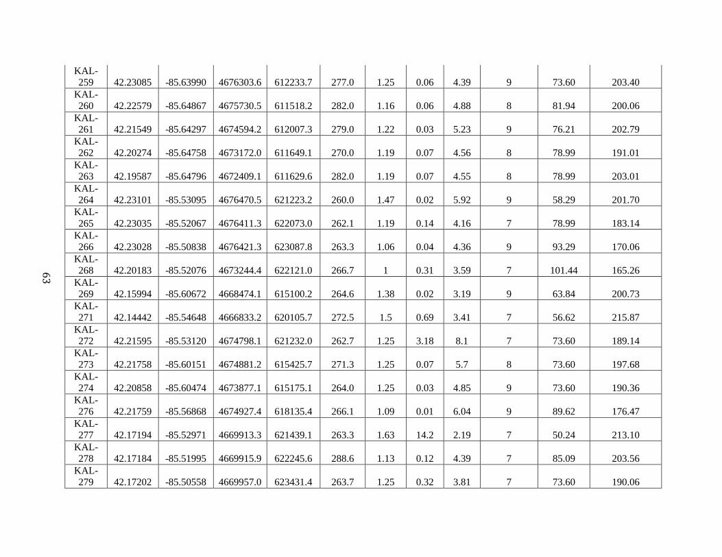
63

KAL-

259 42.23085 -85.63990 4676303.6 612233.7 277.0 1.25 0.06 4.39 9 73.60 203.40

KAL-

260 42.22579 -85.64867 4675730.5 611518.2 282.0 1.16 0.06 4.88 8 81.94 200.06

KAL-

261 42.21549 -85.64297 4674594.2 612007.3 279.0 1.22 0.03 5.23 9 76.21 202.79

KAL-

262 42.20274 -85.64758 4673172.0 611649.1 270.0 1.19 0.07 4.56 8 78.99 191.01

KAL-

263 42.19587 -85.64796 4672409.1 611629.6 282.0 1.19 0.07 4.55 8 78.99 203.01

KAL-

264 42.23101 -85.53095 4676470.5 621223.2 260.0 1.47 0.02 5.92 9 58.29 201.70

KAL-

265 42.23035 -85.52067 4676411.3 622073.0 262.1 1.19 0.14 4.16 7 78.99 183.14

KAL-

266 42.23028 -85.50838 4676421.3 623087.8 263.3 1.06 0.04 4.36 9 93.29 170.06

KAL-

268 42.20183 -85.52076 4673244.4 622121.0 266.7 1 0.31 3.59 7 101.44 165.26

KAL-

269 42.15994 -85.60672 4668474.1 615100.2 264.6 1.38 0.02 3.19 9 63.84 200.73

KAL-

271 42.14442 -85.54648 4666833.2 620105.7 272.5 1.5 0.69 3.41 7 56.62 215.87

KAL-

272 42.21595 -85.53120 4674798.1 621232.0 262.7 1.25 3.18 8.1 7 73.60 189.14

KAL-

273 42.21758 -85.60151 4674881.2 615425.7 271.3 1.25 0.07 5.7 8 73.60 197.68

KAL-

274 42.20858 -85.60474 4673877.1 615175.1 264.0 1.25 0.03 4.85 9 73.60 190.36

KAL-

276 42.21759 -85.56868 4674927.4 618135.4 266.1 1.09 0.01 6.04 9 89.62 176.47

KAL-

277 42.17194 -85.52971 4669913.3 621439.1 263.3 1.63 14.2 2.19 7 50.24 213.10

KAL-

278 42.17184 -85.51995 4669915.9 622245.6 288.6 1.13 0.12 4.39 7 85.09 203.56

KAL-

279 42.17202 -85.50558 4669957.0 623431.4 263.7 1.25 0.32 3.81 7 73.60 190.06

64

KAL-

280 42.17203 -85.49624 4669971.4 624203.3 270.1 0.81 0.33 3.28 5 137.34 132.71

KAL-

281 42.18019 -85.50953 4670857.9 623089.4 266.1 1.19 0.23 3.74 7 78.99 187.10

KAL-

282 42.18389 -85.51560 4671260.2 622581.1 268.8 1.19 0.15 3.74 7 78.99 189.84

KAL-

283 42.19269 -85.51614 4672236.7 622520.0 265.8 1.63 0.1 3.93 8 50.24 215.54

KAL-

285 42.16097 -85.60907 4668584.9 614903.9 264.6 1.06 0.27 4.01 7 93.29 171.28

KAL-

287 42.16309 -85.57553 4668866.0 617670.4 263.0 1.25 0.03 6.87 9 73.60 189.45

KAL-

288 42.16291 -85.57969 4668840.5 617327.4 266.7 1.19 0.08 6.19 8 78.99 187.71

KAL-

291 42.15958 -85.55122 4668510.3 619685.6 268.0 1.38 0.31 4.31 7 63.84 204.16

KAL-

295 42.15983 -85.56766 4668515.1 618326.9 274.0 1.34 0.1 5.81 8 66.59 207.41

KAL-

296 42.15398 -85.57310 4667858.0 617888.4 267.0 1.41 0.05 3.77 9 61.89 205.11

KAL-

298 42.17156 -85.56941 4669815.2 618160.5 269.0 1.31 0.12 5.43 8 68.80 200.20

KAL-

306 42.22610 -85.60450 4675823.1 615163.1 277.0 1.22 0.03 5.49 9 76.21 200.79

KAL-

310 42.21588 -85.54286 4674773.4 620269.4 271.0 1.19 0.07 5.01 8 78.99 192.01

KAL-

313 42.12841 -85.54015 4665064.9 620659.3 266.0 1.36 0.06 8.99 9 65.19 200.81

KAL-

314 42.12972 -85.52583 4665230.7 621840.4 262.0 1.94 0.3 4.59 7 39.12 222.88

KAL-

315 42.24536 -85.66759 4677878.3 609923.1 301.0 1.03 0.03 4.55 9 97.22 203.78

KAL-

317 42.24352 -85.69229 4677642.4 607888.4 296.0 1.09 0.07 4.05 8 89.62 206.38

KAL-

318 42.24500 -85.70048 4677796.4 607210.2 307.0 0.94 0.57 3.63 7 110.88 196.12

65

KAL-

319 42.24625 -85.71158 4677921.3 606292.4 304.0 0.78 0.19 3.06 7 145.00 159.00

KAL-

320 42.24416 -85.72573 4677671.7 605128.5 295.0 1.09 0.04 3.36 8 89.62 205.38

KAL-

321 42.24298 -85.67429 4677605.4 609374.4 292.0 1.09 0.17 5.86 7 89.62 202.38

KAL-

322 42.23610 -85.67528 4676840.2 609304.6 289.0 1.13 0.04 6.09 9 85.09 203.91

KAL-

325 42.22211 -85.65791 4675309.2 610762.3 291.0 1.13 0.12 4.75 7 85.09 205.91

KAL-

326 42.21868 -85.66446 4674919.9 610227.7 290.0 1.09 0.03 6.14 9 89.62 200.38

KAL-

327 42.21374 -85.67144 4674362.4 609660.2 293.0 1.06 0.11 6.11 7 93.29 199.71

KAL-

328 42.20674 -85.67982 4673574.4 608980.5 280.0 1.22 0.13 4.67 7 76.21 203.79

KAL-

329 42.20263 -85.68602 4673110.1 608475.7 280.0 1.19 0.02 4.57 9 78.99 201.01

KAL-

330 42.18646 -85.64826 4671363.4 611621.5 284.0 1.13 0.18 4.43 7 85.09 198.91

KAL-

332 42.21758 -85.67349 4674786.1 609484.3 309.0 0.91 18.99 2.92 7 116.17 192.83

KAL-

333 42.22187 -85.67578 4675259.5 609287.9 281.0 0.81 0.07 5.96 8 137.34 143.66

KAL-

334 42.22530 -85.67266 4675644.4 609539.5 267.0 0.81 21.79 3.14 7 137.34 129.66

KAL-

335 42.20203 -85.54604 4673231.0 620033.2 273.0 1.03 0.03 7.51 9 97.22 175.78

KAL-

336 42.20177 -85.54647 4673201.6 619998.1 271.0 1.03 0.02 8.27 7 97.22 173.78

KAL-

337 42.21534 -85.54692 4674707.7 619935.3 271.0 1.06 0.09 6.73 8 93.29 177.71

KAL-

338 42.21506 -85.54697 4674676.5 619931.7 268.0 1.19 0.06 7.45 8 78.99 189.01

KAL-

339 42.21518 -85.55969 4674672.1 618881.6 267.0 0.94 0.04 6.02 9 110.88 156.12

66

KAL-

341 42.20987 -85.56516 4674074.8 618440.0 265.0 1.22 0.05 5.93 9 76.21 188.79

KAL-

342 42.21145 -85.56727 4674247.3 618262.9 285.0 1.19 0.03 7.88 9 78.99 206.01

KAL-

343 42.21308 -85.56791 4674427.4 618207.0 270.0 1.23 0.44 4.55 6 75.32 194.68

KAL-

344 42.21449 -85.56914 4674582.3 618102.9 273.0 1.13 0.12 8.73 7 85.09 187.91

KAL-

345 42.23385 -85.62379 4676657.7 613557.3 279.0 1.13 0.04 4.88 9 85.09 193.91

KAL-

346 42.22678 -85.62082 4675876.6 613815.0 273.0 1.09 0.08 4.98 8 89.62 183.38

KAL-

347 42.21283 -85.62822 4674317.8 613229.3 275.0 1.09 0.03 5.27 9 89.62 185.38

KAL-

348 42.19935 -85.63268 4672815.2 612885.1 267.0 1.22 0.26 5.56 7 76.21 190.79

KAL-

349 42.18541 -85.62863 4671272.7 613244.4 283.0 1.16 24.63 3.38 7 81.94 201.06

KAL-

350 42.18636 -85.64422 4671357.6 611955.3 289.0 1.19 0.03 4.58 9 78.99 210.01

KAL-

351 42.15685 -85.63441 4668093.9 612817.8 264.0 1.06 0.04 5.3 9 93.29 170.71

KAL-

352 42.22653 -85.62848 4675838.7 613183.3 290.0 1.16 0.04 6.04 9 81.94 208.06

KAL-

353 42.12023 -85.58772 4664090.5 616742.5 264.0 1.31 0.09 5.34 8 68.80 195.20

KAL-

354 42.20063 -85.56074 4673055.0 618822.2 265.0 1.47 0.2 3.56 7 58.29 206.71

KAL-

355 42.21855 -85.56500 4675038.9 618437.0 276.0 0.88 0.13 6.17 8 121.91 154.09

KAL-

356 42.24961 -85.61491 4678419.5 614261.6 270.0 1.16 0.05 3.93 9 81.94 188.06

KAL-

357 42.25155 -85.60281 4678651.2 615256.2 278.0 1.09 0.04 6.66 9 89.62 188.38

KAL-

358 42.25388 -85.58891 4678928.8 616398.6 262.0 1.03 0.03 3.94 9 97.22 164.78

67

KAL-

359 42.25338 -85.57949 4678886.2 617176.6 280.0 1.24 0.05 3.66 9 74.45 205.55

KAL-

360 42.25281 -85.55993 4678850.0 618791.2 264.0 1.16 0.06 5.6 8 81.94 182.06

KAL-

361 42.25068 -85.53154 4678653.5 621137.2 258.0 1 0.11 3.68 7 101.44 156.56

KAL-

05 -42.17196 -85.64826 4669753.2 611647.4 274.1 1.00 0.09 4.12 8 101.44 172.67

KAL-

54 -42.18390 -85.64807 4671079.7 611641.3 273.9 1.19 0.02 4.66 9 78.99 194.88

KAL-

362 42.24522 -85.48212 4678118.7 625224.9 266.0 1.09 0.1 6.58 8 89.62 176.38

KAL-

363 42.23783 -85.48188 4677298.5 625259.3 263.0 1.34 2.76 3.83 7 66.59 196.41

KAL-

365 42.20115 -85.48108 4673226.8 625397.9 265.0 1.19 0.61 3.28 7 78.99 186.01

KAL-

366 42.19313 -85.48115 4672336.2 625407.9 261.0 1.16 0.04 3.91 9 81.94 179.06

KAL-

367 42.18673 -85.48111 4671625.6 625423.9 267.0 1.09 0.02 3.66 9 89.62 177.38

KAL-

368 42.14270 -85.48038 4666737.8 625571.2 261.0 0.88 0.64 5.28 7 121.91 139.09

KAL-

369 42.22116 -85.57427 4675315.8 617667.0 245.0 1.16 0.12 5.76 7 81.94 163.06

KAL-

370 42.20102 -85.52767 4673145.3 621551.8 1.13 0.1 4.43 8 85.09 -85.09

KAL-

372 42.18828 -85.50637 4671760.3 623334.7 1.19 1.8 4.89 7 78.99 -78.99

KAL-

373 42.20538 -85.66615 4673440.9 610111.3 284.0 0.94 0.03 6.09 9 110.88 173.12

KAL-

374 42.19422 -85.66682 4672200.9 610075.4 284.0 0.94 0.1 5 8 110.88 173.12

KAL-

375 42.21709 -85.67109 4674734.8 609683.3 281.0 1.06 0.05 3.59 9 93.29 187.71

KAL-

376 42.20137 -85.69118 4672963.7 608051.9 280.0 1 0.04 5.22 9 101.44 178.56

68

KAL-

377 42.20124 -85.70637 4672930.1 606798.0 279.0 0.72 0.03 4.05 9 162.69 116.31

KAL-

378 42.20338 -85.71505 4673156.9 606077.9 288.0 0.72 0.02 7.78 9 162.69 125.31

KAL-

379 42.21270 -85.68755 4674226.3 608332.2 285.0 0.78 0.02 8.36 9 145.00 140.00

KAL-

380 42.21859 -85.68714 4674880.8 608356.0 289.0 0.94 0.05 5.41 8 110.88 178.12

KAL-

382 42.22555 -85.68637 4675654.6 608407.6 291.0 0.81 0.08 3.79 8 137.34 153.66

KAL-

384 42.21931 -85.67112 4674981.3 609677.0 304.0 0.81 0.06 4.55 8 137.34 166.66

KAL-

385 42.22132 -85.67107 4675204.5 609677.6 299.0 0.78 0.07 5.77 8 145.00 154.00

KAL-

386 42.22666 -85.67176 4675796.6 609611.4 299.0 0.94 0.02 5.38 9 110.88 188.12

KAL-

387 42.23834 -85.70645 4677049.4 606728.9 293.0 0.75 0.03 5.38 9 153.42 139.58

KAL-

388 42.23420 -85.70617 4676590.1 606759.0 298.0 0.72 2.44 2.81 7 162.69 135.31

KAL-

389 42.22728 -85.70630 4675821.6 606759.9 293.0 0.75 0.08 3.4 8 153.42 139.58

KAL-

391 42.20835 -85.70712 4673718.6 606724.2 280.0 0.72 0.13 3.22 7 162.69 117.31

KAL-

392 42.21114 -85.72837 4674002.0 604965.4 287.0 0.75 0.04 5.91 8 153.42 133.58

KAL-

393 42.21526 -85.73552 4674450.7 604368.4 288.0 0.75 0.04 3.97 8 153.42 134.58

KAL-

394 42.21561 -85.74890 4674473.3 603263.4 292.0 1 0.09 3.53 8 101.44 190.56

KAL-

396 42.19617 -85.68716 4672391.4 608392.7 282.0 1.03 0.05 5.29 8 97.22 184.78

KAL-

397 42.18650 -85.68708 4671317.8 608415.8 275.0 1 0.1 4.91 8 101.44 173.56

KAL-

398 42.17928 -85.68968 4670512.8 608213.4 275.0 1.03 0.07 3.35 8 97.22 177.78

69

KAL-

399 42.17219 -85.68750 4669728.3 608405.5 275.0 1.13 0.1 5.05 8 85.09 189.91

KAL-

45 -42.17193 -85.76518 4669604.3 601990.3 269.2 0.78 0.01 5.300 9 145.00 124.16

KAL-

46 -42.17189 -85.75957 4669606.6 602453.1 278.9 0.75 0.04 5.558 9 153.42 125.48

KAL-

47 -42.17185 -85.75216 4669610.2 603065.5 280.2 0.75 0.01 4.905 9 153.42 126.74

KAL-

48 -42.17189 -85.74082 4669629.0 604002.1 287.1 0.81 0.02 4.108 9 137.34 149.71

KAL-

49 -42.17193 -85.73248 4669643.0 604690.7 299.3 0.88 0.07 4.280 8 121.91 177.36

KAL-

50 -42.17228 -85.72404 4669692.7 605387.6 288.5 1.06 0.0 5.50 9 93.29 195.22

KAL-

10 -42.17351 -85.72039 4669833.5 605686.4 286.6 1.00 0.10 4.570 8 101.44 185.17

KAL-

11 -42.17113 -85.71623 4669574.3 606034.1 280.4 1.03 0.06 4.950 8 97.22 183.17

KAL-

12 -42.17187 -85.71058 4669664.3 606499.6 282.4 1.13 0.06 5.250 9 85.64 196.73

KAL-

13 -42.17157 -85.70696 4669635.4 606799.0 281.8 1.13 0.06 6.490 9 85.09 196.68

KAL-

14 -42.17207 -85.69178 4669709.8 608052.2 274.7 1.21 0.02 5.100 9 77.58 197.15

KAL-

08 -42.17191 -85.68189 4669704.5 608869.8 274.4 1.13 0.02 4.800 9 85.09 189.36

KAL-

07 -42.17191 -85.67231 4669716.4

609660.6 274.8 1.00 0.07 4.602 8 101.44 173.38

KAL-

09 -42.17192 -85.66481 4669727.4 610280.2 273.9 1.25 0.07 4.300 9 73.60 200.32

KAL-

06 -42.1719 -85.65915 4669732.6 610747.5 274.6 1.38 0.05 4.175 9 63.84 210.79

KAL-

51 -42.17186 -85.65442 4669734.0 611138.4 273.1 1.13 0.0 5.498 9 85.09 187.99

KAL-

05R -42.172 -85.64808 4669758.8 611661.7 274.1 1.25 0.08 4.137 8 73.60 200.52

70

KAL-

64 -42.18647 -85.75946 4671225.2 602439.1 298.6 0.76 0.03 6.561 9 150.52 148.09

KAL-

63 -42.18649 -85.74759 4671242.0 603419.1 289.2 0.72 0.04 5.811 8 162.69 126.55

KAL-

62 -42.18649 -85.73707 4671254.7 604287.9 288.9 0.76 0.07 4.988 8 150.52 138.43

KAL-

66 -42.18641 -85.72724 4671257.4 605100.0 302.8 1.02 0.03 4.996 9 99.29 203.48

KAL-

61 -42.18666 -85.72479 4671288.1 605301.3 306.4 1.10 0.05 5.224 9 88.45 217.92

KAL-

67 -42.18649 -85.72087 4671274.6 605625.8 307.0 1.06 0.12 5.245 7 93.29 213.71

KAL-

59 -42.18652 -85.71284 4671287.5 606288.9 310.7 0.78 0.03 8.351 9 145.00 165.71

KAL-

58 -42.18654 -85.70414 4671300.5 607006.9 297.4 0.78 0.13 4.622 7 145.00 152.43

KAL-

57 -42.18658 -85.69529 4671316.3 607737.6 284.9 0.92 0.10 4.864 8 114.36 170.57

KAL-

56 -42.18658 -85.68560 4671328.9 608538.2 278.8 0.84 0.15 5.843 7 129.68 149.13

KAL-

60 -42.18648 -85.68427 4671319.5 608648.1 279.0 1.13 0.07 5.639 8 85.09 193.89

KAL-

55 -42.1864 -85.67445 4671323.2 609458.8 278.2 1.1 0.06 4.532 8 88.10 190.13

KAL-

52 -42.18639 -85.66749 4671330.9 610033.7 277.3 1.09 0.01 7.578 9 89.62 187.68

KAL-

53 -42.1864 -85.66018 4671342.0 610637.1 276.6 1.03 0.05 4.763 9 96.81 179.76

KAL-

54 -42.1839 -85.64807 4671079.7 611641.3 273.9 1.19 0.02 4.662 9 78.99 194.88

KAL-

400 42.18008 -85.64802 4670655.3 611652.6 275.0 1.25 33.65 3.51 7 73.60 201.40

KAL-

401 42.17202 -85.64803 4669760.3 611665.9 279.0 0.94 0.17 3.41 7 110.88 168.12

KAL-

402 42.16059 -85.64767 4668491.7 611715.8 274.0 1.03 0.06 4.44 8 97.22 176.78

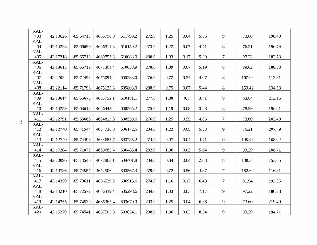
71

KAL-

403 42.13626 -85.64719 4665790.8 611798.2 272.0 1.25 0.04 5.56 9 73.60 198.40

KAL-

404 42.14298 -85.66699 4666511.3 610150.2 273.0 1.22 0.07 4.71 8 76.21 196.79

KAL-

405 42.17218 -85.66713 4669753.3 610088.0 280.0 1.03 0.17 5.39 7 97.22 182.78

KAL-

406 42.18615 -85.66719 4671304.4 610058.9 278.0 1.09 0.07 5.19 8 89.62 188.38

KAL-

407 42.22094 -85.72493 4675094.4 605233.0 276.0 0.72 0.54 4.07 8 162.69 113.31

KAL-

408 42.22114 -85.71796 4675125.3 605808.0 288.0 0.75 0.07 5.44 8 153.42 134.58

KAL-

409 42.13614 -85.66676 4665752.1 610181.1 277.0 1.38 0.1 3.71 8 63.84 213.16

KAL-

410 42.14259 -85.68618 4666443.4 608565.2 275.0 1.19 0.08 3.28 8 78.99 196.01

KAL-

411 42.12791 -85.68666 4664812.8 608550.6 276.0 1.25 0.55 4.86 7 73.60 202.40

KAL-

412 42.12740 -85.71544 4664720.0 606172.6 284.0 1.22 0.05 5.33 9 76.21 207.79

KAL-

413 42.12740 -85.74493 4664683.7 603735.2 274.0 0.97 0.04 4.71 9 105.98 168.02

KAL-

414 42.17204 -85.71075 4669682.4 606485.4 282.0 1.06 0.03 5.64 9 93.29 188.71

KAL-

415 42.20096 -85.73540 4672863.1 604401.8 284.0 0.84 0.04 2.68 8 130.35 153.65

KAL-

416 42.19786 -85.74557 4672506.4 603567.3 279.0 0.72 0.56 4.37 7 162.69 116.31

KAL-

417 42.14359 -85.70611 4666529.2 606916.6 274.0 1.16 0.17 6.43 7 81.94 192.06

KAL-

418 42.14210 -85.72572 4666339.4 605298.6 284.0 1.03 0.03 7.17 9 97.22 186.78

KAL-

419 42.14255 -85.74530 4666365.4 603679.9 293.0 1.25 0.04 6.36 9 73.60 219.40

KAL-

420 42.15279 -85.74541 4667502.3 603654.1 288.0 1.06 0.02 8.34 9 93.29 194.71

72

KAL-

421 42.15599 -85.72606 4667881.3 605247.5 282.0 1.09 0.09 5.97 8 89.62 192.38

KAL-

422 42.14962 -85.70630 4667198.7 606890.7 274.0 1.16 0.02 8.04 9 81.94 192.06

KAL-

423 42.24662 -85.73978 4677927.6 603965.3 286.0 1 0.35 2.15 7 101.44 184.56

KAL-

424 42.23422 -85.75540 4676531.8 602696.8 300.0 0.94 0.09 4.5 8 110.88 189.12

KAL-

425 42.23018 -85.74297 4676098.3 603729.0 312.0 0.72 0.05 5.81 8 162.69 149.31

KAL-

426 42.23827 -85.73724 4677003.6 604188.6 284.0 0.75 0.02 4.69 9 153.42 130.58

KAL-

427 42.20832 -85.74642 4673666.8 603480.0 296.0 0.94 0.07 4.68 8 110.88 185.12

KAL-

428 42.19764 -85.75111 4672475.3 603110.2 281.0 0.91 0.08 3.72 8 116.17 164.83

KAL-

429 42.17839 -85.74044 4670350.8 604022.7 316.0 0.88 0.02 4.94 9 121.91 194.09

KAL-

430 42.17917 -85.71159 4670473.0 606404.1 284.0 0.94 0.05 5.46 9 110.88 173.12

KAL-

431 42.16439 -85.74036 4668796.4 604052.3 320.0 0.88 0.02 5.86 9 121.91 198.09

KAL-

432 42.16553 -85.68678 4668989.7 608476.4 277.0 1.16 0.02 4.08 9 81.94 195.06

KAL-

433 42.15961 -85.66746 4668357.2 610082.6 279.0 1.38 0.07 3.67 9 63.84 215.16

KAL-

434 42.21030 -85.66196 4673992.7 610448.7 287.0 1.03 0.06 5.14 8 97.22 189.78

KAL-

436 42.19382 -85.69554 4672119.8 607704.7 288.0 1.19 0.17 5.2 7 78.99 209.01

KAL-

437 42.19247 -85.70633 4671956.4 606816.1 284.0 0.91 0.07 5.02 8 116.17 167.83

KAL-

438 42.19331 -85.71132 4672043.4 606402.7 294.0 0.94 0.08 4.3 8 110.88 183.12

KAL-

439 42.25080 -85.65750 4678495.4 610746.0 295.0 1.13 0.05 6.36 9 85.09 209.91

73

KAL-

440 42.25135 -85.67712 4678531.2 609126.5 296.0 0.84 0.12 3.8 8 130.35 165.65

KAL-

441 42.25514 -85.69670 4678927.1 607504.9 296.0 1.09 0.07 3.76 8 89.62 206.38

KAL-

443 42.25292 -85.71526 4678657.3 605977.6 305.0 0.72 0.07 4.86 8 162.69 142.31

KAL-

444 42.25367 -85.72586 4678727.5 605102.0 294.0 1.09 0.16 3.97 7 89.62 204.38

KAL-

445 42.24472 -85.75508 4677698.1 602706.1 288.0 0.78 0.02 5.29 9 145.00 143.00

KAL-

446 42.23866 -85.71370 4677075.9 606130.2 282.0 0.72 0.05 5.1 8 162.69 119.31

KAL-

447 42.12228 -85.64674 4664239.2 611860.0 273.0 1.22 0.08 6.88 8 76.21 196.79

KAL-

448 42.12051 -85.66620 4664017.3 610254.5 278.0 1.06 0.04 5.87 9 93.29 184.71

KAL-

449 42.12064 -85.68614 4664006.2 608606.0 273.0 1.25 0.08 5.27 8 73.60 199.40

KAL-

450 42.12060 -85.69720 4663987.8 607691.8 275.0 1.22 0.07 4.51 8 76.21 198.79

KAL-

451 42.12058 -85.71490 4663963.4 606228.7 281.0 1.19 0.12 3.83 8 78.99 202.01

KAL-

452 42.11979 -85.74467 4663839.1 603769.1 284.0 0.94 0.03 4.13 9 110.88 173.12

KAL-

453 42.14161 -85.76421 4666238.3 602118.8 306.0 0.84 0.03 5.77 9 130.35 175.65

KAL-

454 42.19365 -85.74067 4672045.0 603978.7 297.0 0.88 0.12 3.57 8 121.91 175.09

KAL-

455 42.12981 -85.52579 4665240.7 621843.5 265.0 1.53 0.04 3.83 9 55.03 209.97

KAL-

456 42.13997 -85.51086 4666390.3 623057.8 261.0 2.16 0.11 3.19 7 33.52 227.48

KAL-

461 42.21995 -85.66428 4675061.1 610240.4 290.0 1.06 0.3 2.87 7 93.29 196.71

KAL-

462 42.22412 -85.65714 4675533.4 610822.4 285.0 0.84 0.04 3.73 9 130.35 154.65

74

KAL-

463 42.24885 -85.62888 4678316.5 613110.5 271.0 0.94 0.06 6.49 8 110.88 160.12

KAL-

464 42.24090 -85.63589 4677424.5 612546.3 281.0 0.84 0.03 4.17 9 130.35 150.65

KAL-

465 42.22834 -85.72306 4675918.4 605375.1 278.0 0.81 0.31 2.59 7 137.34 140.66

KAL-

466 42.23172 -85.72612 4676289.9 605116.9 288.0 0.88 0.06 4.59 8 121.91 166.09

KAL-

467 42.23594 -85.72173 4676763.9 605472.2 288.0 0.94 0.1 4.84 8 110.88 177.12

KAL-

468 42.15111 -85.52364 4667608.9 621980.3 271.0 1.88 0.1 3.02 7 40.92 230.08

KAL-

469 42.15369 -85.49657 4667934.4 624211.9 273.0 1.06 0.09 3.88 8 93.29 179.71

Mapping Bedrock Topography of the Portage and Schoolcraft ...

Documents

Transcript of Mapping Bedrock Topography of the Portage and Schoolcraft ...