Mapamatics of Images

Multi-band images are picture sandwiches partitioned into pixels by remote sensing.

A raster map is a ‘paint-by-number’ grid layer for GIS.

The present concern is to recast a multi-band image in the manner of a raster map for GIS while retaining or improving its overall utility.

ASTER-1

.556 micrometers

ASTER-2

.661 micrometers

ASTER-3

.807 micrometers

ASTER-4

1.656 micrometers

ASTER-5

2.167 micrometers

ASTER-6

8.291 micrometers

ASTER-7

8.631 micrometers

ASTER-8

9.075 micrometers

ASTER-9

10.657 micrometers

ASTER-10

11.318 micrometers

ASTER-MAP

PSIMAPP ordered overtones

PSIMAPP Progressively Segmented Image Modeling As Poly-Patterns produces Image Models As Grouped Elements (IMAGE).

The grouping process provides an aggregated A-level model consisting of 250 (compound) segments that are numbered in order of overall intensity and recorded as a byte-binary map of segment numbers.

A finer B-level model has several thousand base segments that are nested within A-level segments up to a maximum of 255 B-segments in an A-segment.

Each level has tables of typical signal properties for the segments.

A mapped segment makes a PATTERN,and patterns within patterns are POLYPATTERNS.

Tonal transfer tables translate typical signals for A-level segments into palettes for pseudo-color images.

Amplifies major messages contained in the data.

PSIMAPP

Diminishes minor messages included in the data (smoothing filter).

Promotes pictorial parsimony (data compression)

Facilitates analysis of (I4C)

Image ContrastImage ContentImage ChangeImage Context

Kinds of Data

Spectral data (remote sensing)

Synoptic environmental indicators

LANDSAT MSS band 1

Central Pennsylvania 1991

LANDSAT MSS band 2

Central Pennsylvania 1991

LANDSAT MSS band 4

Central Pennsylvania 1991

The pattern pictures give considerable control of colors for creative coloration.

Each segment pattern can be color coded individually.

There are 4 stages to pattern processing.

Spreading (250) proto-patterns through signal space.Populating (250) preliminary patterns.Splitting preliminary patterns into primary patterns (B-level).Sorting primary patterns into (A-level) polypatterns.

Formulation of poly-pattern IMAGE model is done with PSISCANS program module.

PSIBRITE program module makes BRS table of relative intensities for signal bands (brightness), and BRI table of integrative image indexes such as modified NDVI (normalized difference vegetation index).

PSITONES program module makes tonal transfer tables (CLR and TRL) for colorized pattern pictures that mimic image enhancements of remote sensing for rendering with both freeware (MultiSpec or ArcExplorer) and commercial (ArcGIS) GIS software.

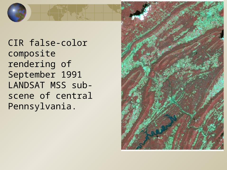
CIR false-color composite rendering of September 1991 LANDSAT MSS sub-scene of central Pennsylvania.

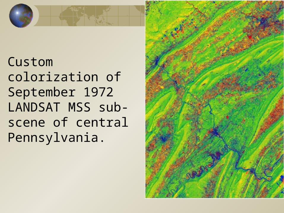
Custom colorization ofSeptember 1972LANDSAT MSS sub-scene of central Pennsylvania.

Red=Amphibian; Green=Turtle; Blue=Fish

Classification of Content

SupervisedUnsupervisedInterpretiveThematic transforms

Supervised classification of water using PSITHEME adaptive advisor module

Classification with PSITHEME works at the pattern level rather than the pixel level, and is thus in the nature of a hybrid between conventional supervised and unsupervised modes.

PSITHEME produces a thematic transform to colorize A-level patterns according to thematic category. A conventional thematic raster map can also be generated with PSICODES module if desired.

Interpretive classification of habitat.

Light gray= viable lowland

Med gray= viable upland

Dark gray=degraded lowland

Black= biotically impoverished

Using ArcGIS with pattern pictures, interactive interpretive classification can be done either by overlay operations or by on-screen digitizing.

Change detection and analysis.

Multi-temporal composite

PSIMAPP compression makes it more practical to combine bands from multiple dates into a multi-date (multi-temporal) composite image that shows additional details in changed areas.

Pattern-based change indicators such as scaled band differences and change vectors are less noisy than pixel-based counterparts due to smoothing from segmentation.

Change with landscape context

Pattern-based change indicators can be set into the context of a pattern picture.

Types of change

Multiple change indicators can be assembled as bands of image-structured data for modeling of change patterns. Then coloration of pattern pictures can be used to distinguished different types of change.

Change Advances

Spatial matching vs. signal matching.

Change sequences/series.

Instead of doing direct detection of differences, patterns enable a special indirect kind of change detection by comparison of pattern positions in the different dates. Perturbation of spatial correspondence can be translated into indicators of change even if the signals are of somewhat different kinds between occasions.

One poly-pattern model for a pair of occasions is chosen as the base occasion for comparison. Let the kth A-level pattern for the base occasion be denoted as ↓PPk and let ↑PPi denote the ith A-level pattern for the other occasion to be linked (link occasion) by pattern matching. Pattern ↓PPk occupies a particular set of pixel positions for the base occasion. These same positions are scanned for the link occasion to determine the pattern ↑PPi that occurs most frequently in this subset of pixels. This modal pattern becomes the counterpart of ↓PPk which we denote as ↓PPk►↑PPi.

Every pixel for the link occasion thus has two patterns associated with it. One of these is its own pattern ↑PPn and the other is the pattern ↑PPi that is expected to occur there on the basis of pattern matching as ↓PPk►↑PPi from the base occasion. Euclidean distance in signal space between ↑PPn and ↑PPi is then computed as a change vector length.

Change indicators from more than two occasions can be integrated into the set of pattern models for appropriate coloration to distinguish times of onset for change and recoveries.

Landscape Context

DIStribution of POSITION (i.e., DISPOSITION) among patterns can be explored to further elucidate spatial structure of the landscape.

Disposition of pattern 6 (left)

and 7 (right).

Joint disposition of patterns 6 & 7.

Differences in edge affinities (juxtaposition or adjacency) can serve to guide exploration of disposition.

Joint disposition of patterns 3 and 6.

Presence of patterns that are strongly situated with strong edge affinities suggest generations of generalization for patterns using both signal similarity and edge affinity.

Pattern generalization (231 on right side)

Panel Pattern ProfilesLandscapes often have characteristic composition in terms of component patterns in a vicinity. Such landscape mosaics can be analyzed by compiling profiles of pattern frequencies in square panels of pixels. Multi-scale analysis can be accomplished by using panels of different sizes. Second-order pattern recognition can be achieved by choosing panels from an area of interest as training sets.

Gray-tone representation of segment number at 90% cumulative frequency in 10x10 panels of pixels.

Compositional Consistency Components

Some subsets of patterns constitute intensity variants of similar signal constituents. In vector terms, these are patterns of like direction in signal space but having different vector lengths. In familiar terms, these are similar environmental features having different “illumination” intensities. Several such patterns may represent features for which all signals are of similar strength, but with different patterns having different overall intensity. It may be of interest to render such patterns distinctively in pattern pictures. This context can be addressed in terms of rank range runs and levels of partially ordered sets (POSETS).

Pattern picture showing senescent herbaceous vegetation in the valleys as light tones.

Restoration, Residuals, and Detrending

The B-level pattern model provides for somewhat smoothed restoration of image signal bands.The spatial distribution and relative magnitudes for errors of approximation can be mapped.The model can also be used for multivariate detrending in spatial statistics.

Restored band 2 (red) of September 1991 LANDSAT MSS image of central Pennsylvania with additional saturation stretching.

Residuals for Sept. 1991 LANDSAT MSS image of central Pennsylvania

Principal Pattern Properties

Signal structure of patterns can be investigated by compiling a frequency weighted covariance matrix from central signal vectors of patterns. Characteristic values and characteristic vectors are then computed in the manner of conventional principal components. Pattern pictures can then be rendered in terms of these principal properties.

Image of second A-level principal component for September 1991 Landsat MSS image of central Pennsylvania.

Contact

Dr. Wayne L. Myers

Prof. of Forest BiometricsDirector, Office for Remote Sensing and Spatial Information ResourcesPenn State Universitywlm@psu.edu