Volatility

• Many economic series, and most financial series, display conditional volatility – The conditional variance changes over time – There are periods of high volatility

• When large changes frequently occur

– And periods of low volatility • When large changes are less frequent

Weekly Stock Prices Levels and Returns

050

010

0015

00sp

1950w1 1960w1 1970w1 1980w1 1990w1 2000w1 2010w1t

-20

-10

010

20r

1950w1 1960w1 1970w1 1980w1 1990w1 2000w1 2010w1t

Conditional Mean

• The conditional mean of y is

• The regression error is mean zero and unforecastable

( )1| −ΩttyE

( ) 0| 1 =Ω −tteE

Conditional Variance

• The conditional variance of y is

• The squared regression error can be forecastable

( ) ( )( )( )( )1

21

211

|

|||var

−

−−−

Ω=

ΩΩ−=Ω

tt

tttttt

eEyEyEy

Forecastable Conditional Variance

• If the squared error is forecastable, then the conditional variance is time-varying and correlated. – The magnitude of changes is predictable – The sign is not predictable

Stock returns are unpredictable

-0.0

50.

000.

050.

10A

utoc

orre

latio

ns o

f r

0 10 20 30 40Lag

Bartlett's formula for MA(q) 95% confidence bands

Prob > F = 0.3009 F( 4, 3115) = 1.22

( 4) L4.r = 0 ( 3) L3.r = 0 ( 2) L2.r = 0 ( 1) L.r = 0

. testparm L(1/4).r

_cons .1337402 .0410395 3.26 0.001 .053273 .2142074 L4. -.0298138 .0264335 -1.13 0.259 -.0816427 .0220151 L3. -.0044898 .0282283 -0.16 0.874 -.0598378 .0508581 L2. .0466548 .0273551 1.71 0.088 -.0069811 .1002907 L1. -.01737 .032557 -0.53 0.594 -.0812053 .0464653 r r Coef. Std. Err. t P>|t| [95% Conf. Interval] Robust

Root MSE = 2.0793 R-squared = 0.0033 Prob > F = 0.3009 F( 4, 3115) = 1.22Linear regression Number of obs = 3120

. reg r L(1/4).r,r

Squared Returns are predictable

Prob > F = 0.0000 F( 4, 3115) = 9.72

( 4) L4.y = 0 ( 3) L3.y = 0 ( 2) L2.y = 0 ( 1) L.y = 0

. testparm L(1/4).y

_cons 2.282243 .3480455 6.56 0.000 1.599821 2.964665 L4. .0517234 .0506949 1.02 0.308 -.0476755 .1511222 L3. .125441 .0364307 3.44 0.001 .0540103 .1968717 L2. .0627729 .0308486 2.03 0.042 .0022873 .1232586 L1. .2332184 .1248813 1.87 0.062 -.0116395 .4780763 y y Coef. Std. Err. t P>|t| [95% Conf. Interval] Robust

Root MSE = 11.618 R-squared = 0.1092 Prob > F = 0.0000 F( 4, 3115) = 9.72Linear regression Number of obs = 3120

. reg y L(1/4).y,r

(1 missing value generated). gen y=(r-.1334364)^2

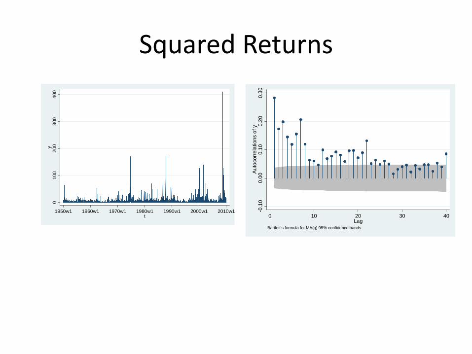
Squared Returns

-0.1

00.

000.

100.

200.

30A

utoc

orre

latio

ns o

f y

0 10 20 30 40Lag

Bartlett's formula for MA(q) 95% confidence bands

010

020

030

040

0y

1950w1 1960w1 1970w1 1980w1 1990w1 2000w1 2010w1t

ARCH

• Robert Engle (1982) proposed a model for the conditional variance – AutoRegressive Conditional

Heteroskedasticity – “ARCH” now describes volatility

models

• Nobel Prize 2003

ARCH(1) Model

• α>0 means that the conditional variance is high when the lagged squared error is high

• Large errors (either sign) today mean high expected errors (in magnitude) tomorrow.

• Small magnitude errors forecast next period small magnitude errors.

( )

00

|var 211

2

≥>

+=Ω=

+=

−−

αω

αωσ

µ

tttt

tt

eeey

Unconditional variance

• A property of expectations is that expected (average) conditional expectations are unconditional expectations.

• So the average conditional variance is the average variance – the variance of the regression error.

• Solving for the variance: ( ) ( ) 22

122 ασωαωσσ +=+== −tt eEE

αωσ−

=1

2

• Rewriting, this implies

• Substituting into ARCH(1) equation

or • This shows that the conditional variance is a

combination of the unconditional variance, and the deviation of the squared error from its average value.

( ) 21

22 1 −+−= tt eασασ

( )ασω −= 12

( )221

22 σασσ −+= −tt e

ARCH(1) as AR(1) in squares

• The model

implies the regression where u is white noise • Thus e-squared is an AR(1)

( ) ( ) 211

21 ||var −−− +=Ω=Ω ttttt eeEe αω

ttt uee ++= −2

12 αω

Estimation

• .arch r, arch(1)

_cons 2.926873 .0686021 42.66 0.000 2.792416 3.061331 L1. .3006982 .0216209 13.91 0.000 .2583219 .3430745 arch ARCH _cons .1996426 .0314495 6.35 0.000 .1380027 .2612825r r Coef. Std. Err. z P>|z| [95% Conf. Interval] OPG

Log likelihood = -6525.268 Prob > chi2 = .Distribution: Gaussian Wald chi2(.) = .Sample: 1950w2 - 2010w5 Number of obs = 3124

ARCH family regression

Variance Forecast

• Given the parameter estimates, the estimated conditional variance for period t is

• The forecasted out-of-sample variance is

( )212

12 ˆˆˆˆˆˆˆ µαωαωσ −+=+= −− ttt ye

( )221 ˆˆˆˆ µαωσ −+=+ nn y

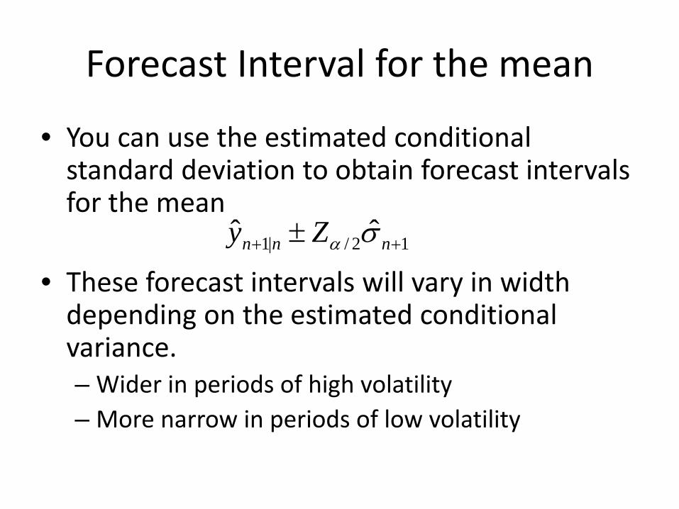
Forecast Interval for the mean

• You can use the estimated conditional standard deviation to obtain forecast intervals for the mean

• These forecast intervals will vary in width depending on the estimated conditional variance. – Wider in periods of high volatility – More narrow in periods of low volatility

12/|1 ˆˆ ++ ± nnn Zy σα

ARCH(p) model

• Allow p lags of squared errors

• Similar to AR(p) in squares • Estimation: ARCH(8)

– .arch r, arch(1/8) – ARCH model with lags 1 through 8

2222

211

2ptpttt

tt

eeeey

−−− ++++=

+=

αααωσ

µ

ARCH(8) Estimates

• .arch r, arch(1/8)

_cons 1.144063 .1001062 11.43 0.000 .9478582 1.340267 L8. .0706622 .0171741 4.11 0.000 .0370015 .1043229 L7. .041083 .0147083 2.79 0.005 .0122553 .0699107 L6. .0811242 .0192012 4.22 0.000 .0434906 .1187578 L5. .0284588 .0171987 1.65 0.098 -.0052501 .0621677 L4. .0912413 .0192753 4.73 0.000 .0534625 .1290202 L3. .1541191 .0225999 6.82 0.000 .1098241 .1984142 L2. .1099957 .0203355 5.41 0.000 .0701388 .1498526 L1. .1867283 .0163376 11.43 0.000 .1547071 .2187495 arch ARCH _cons .2027503 .0290226 6.99 0.000 .1458671 .2596335r r Coef. Std. Err. z P>|z| [95% Conf. Interval] OPG

Log likelihood = -6368.552 Prob > chi2 = .Distribution: Gaussian Wald chi2(.) = .Sample: 1950w2 - 2010w5 Number of obs = 3124

ARCH family regression

ARCH needs many lags

• Notice that we included 8 lags, and all appeared significant.

• This is commonly observed in estimated ARCH models – The conditional variance appears to be a function

of many lagged past squares

GARCH Model

• Tim Bollerslev (1986) – A student of Engle – Current faculty at Duke

proposed the GARCH model to simplify this problem

000

21

21

2

≥>>

++= −−

αωβ

αβσωσ ttt e

GARCH(1,1)

• This makes the variance a function of all past lags:

• It is also smoother than an ARCH model with a small number of lags

( )∑∞

=−−

−−

+=

++=

0

21

21

21

2

jjt

j

ttt

e

e

αωβ

αβσωσ

GARCH(p,q)

• p lags of squared error • q lags of conditional variance

• GARCH(1,1): – .arch r, arch(1) garch(1)

• GARCH(3,2): – .arch r, arch(1/3) garch(1/2)

2211

2211

2ptptqtqtt ee −−−− ++++++= αασβσβωσ

GARCH(1,1)

• Common GARCH features – Lagged variance has large coefficient – Sum of two coefficients very close to (but less than) one

_cons .1207574 .0221764 5.45 0.000 .0772924 .1642223 L1. .8444868 .0117076 72.13 0.000 .8215404 .8674333 garch L1. .1317621 .0094385 13.96 0.000 .113263 .1502613 arch ARCH _cons .1935287 .0296365 6.53 0.000 .1354421 .2516152r r Coef. Std. Err. z P>|z| [95% Conf. Interval] OPG

Log likelihood = -6359.118 Prob > chi2 = .Distribution: Gaussian Wald chi2(.) = .Sample: 1950w2 - 2010w5 Number of obs = 3124

ARCH family regression

GARCH(2,2) for Stock Returns

_cons .1233949 .0428309 2.88 0.004 .0394478 .207342 L2. .2373325 .2478461 0.96 0.338 -.248437 .7231021 L1. .5991681 .2941188 2.04 0.042 .0227059 1.17563 garch L2. -.0277704 .042739 -0.65 0.516 -.1115373 .0559964 L1. .1658834 .0149416 11.10 0.000 .1365984 .1951684 arch ARCH _cons .1913999 .0295859 6.47 0.000 .1334126 .2493872r r Coef. Std. Err. z P>|z| [95% Conf. Interval] OPG

Log likelihood = -6356.166 Prob > chi2 = .Distribution: Gaussian Wald chi2(.) = .Sample: 1950w2 - 2010w5 Number of obs = 3124

ARCH family regression

GARCH(1,1)

• The GARCH(1,1) often fits well, and is a useful benchmark. – Daily, weekly, or monthly asset returns, exchange

rates, or interest rates

Extensions

• There are many extensions of the basic GARCH model, developed to handle a variety of situations – Asymmetric Response – Garch-in-mean – Explanatory variables in variance – Non-normal errors

Asymetric GARCH

• Threshold GARCH

• The last tern is dummy variable for positive lagged errors

• This model specifies that the ARCH effect depends on whether the error was positive or negative – If the error is negative, the effect is α – If the error is positive, the full effect is α+γ

( )01 12

12

12

12 >+++= −−−− ttttt eee γαβσωσ

TARCH estimation • .arch r, arch(1) tarch(1) garch(1) • Negative errors have coefficient of 0.19 • Positive errors have coefficient of 0.05 • Negative returns increase volatility much more than positive returns

_cons .1540714 .0219836 7.01 0.000 .1109843 .1971585 L1. .8437111 .0132294 63.78 0.000 .817782 .8696403 garch L1. -.1408097 .0160892 -8.75 0.000 -.1723439 -.1092754 tarch L1. .1879679 .0154078 12.20 0.000 .1577692 .2181665 arch ARCH _cons .1474826 .0313132 4.71 0.000 .0861099 .2088552r r Coef. Std. Err. z P>|z| [95% Conf. Interval] OPG

Log likelihood = -6332.433 Prob > chi2 = .Distribution: Gaussian Wald chi2(.) = .Sample: 1950w2 - 2010w5 Number of obs = 3124

ARCH family regression

Leverage Effect

• This model describes what is called the “leverage effect” – A negative shock to equity increases the ratio

debt/equity of investors – This increases the leverage of their portfolios – This increases risk, and the conditional variance – Negative shocks have stronger effect on variance

than positive shocks

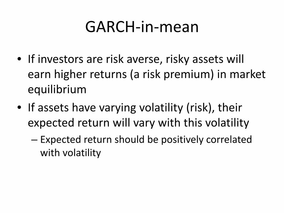
GARCH-in-mean

• If investors are risk averse, risky assets will earn higher returns (a risk premium) in market equilibrium

• If assets have varying volatility (risk), their expected return will vary with this volatility – Expected return should be positively correlated

with volatility

GARCH-M model

• .arch arch(1) garch(1) archm

21

21

2

2111

−−

−

++=

++=

ttt

tt

e

ey

αβσωσ

σββ

GARCH-M for Stock Returns

• Marginally positive effect

_cons .1193442 .022376 5.33 0.000 .075488 .1632004 L1. .8450762 .0118319 71.42 0.000 .8218862 .8682662 garch L1. .1315334 .0096454 13.64 0.000 .1126287 .1504381 arch ARCH sigma2 .024739 .0143783 1.72 0.085 -.003442 .0529199ARCHM _cons .1211625 .0512489 2.36 0.018 .0207165 .2216085r r Coef. Std. Err. z P>|z| [95% Conf. Interval] OPG

Log likelihood = -6357.259 Prob > chi2 = 0.0853Distribution: Gaussian Wald chi2(1) = 2.96Sample: 1950w2 - 2010w5 Number of obs = 3124

ARCH family regression

TARCH and GARCH-M

• .arch arch(1) tarch(1) garch(1) archm • archm term appears insignificant

_cons .1565728 .0228305 6.86 0.000 .1118259 .2013197 L1. .8425617 .0137719 61.18 0.000 .8155693 .8695542 garch L1. -.1391533 .0161185 -8.63 0.000 -.1707449 -.1075617 tarch L1. .1872044 .0155283 12.06 0.000 .1567694 .2176393 arch ARCH sigma2 .0059058 .0142042 0.42 0.678 -.021934 .0337456ARCHM _cons .1309694 .0512904 2.55 0.011 .030442 .2314967r r Coef. Std. Err. z P>|z| [95% Conf. Interval] OPG

Log likelihood = -6332.324 Prob > chi2 = 0.6776Distribution: Gaussian Wald chi2(1) = 0.17Sample: 1950w2 - 2010w5 Number of obs = 3124

ARCH family regression

Estimated standard deviation

• Estimated TARCH model • .predict v, variance • .gen s=sqrt(v) • Unconditional variance is 2.1

02

46

810

s

1950w1 1960w1 1970w1 1980w1 1990w1 2000w1 2010w1t

S&P, returns, and standard deviation 2006-2010

24

68

10s

2006w1 2007w1 2008w1 2009w1 2010w1t

600

800

1000

1200

1400

1600

sp

2006w1 2007w1 2008w1 2009w1 2010w1t

-20

-10

010

r

2006w1 2007w1 2008w1 2009w1 2010w1t