1

Manuals for DC programs Installation and manuals common to most programs Installation notes The relationships between programs, and default file names Some notes about input and printout that apply to all programs Notes for use of the graphics subroutines that are common to all programs Publication quality graphs from DCprogs Notes on installation of the CED1401-plus interface for use with CONSAM and CJUMP General purpose programs CVFIT Curve fitting List of equations that are available in CVFIT Direct fit of the Schild equation to data with CVFIT AUTPLOT Automatic (or posh) plotting of queued graphs. AUTPLOT will plot queued graphs (including 3D), histograms or single channel records that have been queued in any other program that offers the option to ‘queue plot’. Normally the queued plots are kept in a plot queue file (default suffix = ‘.plq’), but AUTPLOT will also plot out all or part of a CJUMP.CJD file, the raw data file generated by CJUMP (q.v.) to produce a quick summary of a jump experiment. RANTEST Does a two-sample randomisation test and displays the randomisation distribution. Single channel analysis SCAN Time course fitting of single channels (steady state or jump). EKDIST Fitting of many sorts of distribution to output from SCAN HJCFIT Fitting of rate constants for a specified mechanism to output from SCAN Notes on the theory that underlies HJCFIT CJUMP5 Do concentration jumps, or voltage jumps/ramps on-line CJFIT Average and fit macroscopic jumps (or aligned steady state bursts) CONSAM Digitise continuously (e.g. from tape) a recording (for SCAN) Single channel utilities

2

SCANFIX. Small utility to list, and if necessary correct, the header data in the output files from SCAN (SCAN.SCN files). PLOTSAMP. Stand alone program to plot an entire single channel record with specified number of seconds per page, lines per page, and line separation (on screen or plotter). This can also be done in AUTPLOT. FILTSAMP. Utility to omit points from and/or filter (with a digital Gaussian filter) a continuously sampled record (e.g. consam.dat file, Axon continuous data (.abf) file), or ASCII file Single channel theory programs How to define, or modify, a reaction mechanism (same for all theory programs, and HJCFIT) SCALCS. Calculates macroscopic jump time course and noise spectra (as in Colquhoun & Hawkes, 1977, 1995a,b) SCBST. Calculate properties of bursts of openings (as in Colquhoun & Hawkes, 1982) SCCOR Calculate properties of correlations between open times, shut times, burst lengths, openings within a burst etc. (see (as in Colquhoun & Hawkes, 1987) SCJUMP. Calculates properties of single channel elicited by a concentration jump (as in Colquhoun, Hawkes, Merlushkin & Edmonds,1997) SCSIM Calculates a simulated series of openings and shuttings (steady state or jump), and puts the results in a SCAN.SCN file for analysis by EKDIST or HJCFIT. It can also add noise to make a simulated CONSAM file. Derivations for channel simulations with time-varying concentration (method used in SCSIM)

3

Program Installation guide (see also http://www.ucl.ac.uk/Pharmacology/setup.html) (1) Download INSTALL.EXE into a temporary directory, for example C:\TEMP (2) Make a backup copy of c:\autoexec.bat (which will be modified by installation) (3) Run INSTALL.EXE following the instructions. The default location for the installation is C:\DCPROGS, but any other location/directory name can be chosen. (4) This program will install all the ancillary files that are needed to run the DC programs on your system. It will NOT install either the manuals, or the programs themselves. After running this installation you should download from our web site the latest versions of the manuals and programs (*.exe) that you need. These should go into the main directory (the default name for which is C:\dcprogs). Two other directories will be created, \gino, and \lf90\bin, but you should not touch these.

There is also an UNINSTALL icon , should you ever wish to remove the software from your system. Please note that this will NOT remove the files added after the installation, i.e. the manuals and the programs. You can delete these manually. (5) After installation, reboot the computer. Then go to the DOS prompt, and type the word PATH. You should see c:\dcprogs; c:\lf90\bin; c:\gino as part of the paths that are set when the computer is booted. They should appear in autoexec.bat either as part of a path command, thus PATH= c:\dcprogs; c:\lf90\bin; c:\gino or appended to a previous PATH command, thus SET PATH=%PATH%;C:\FORT90;C:\LF90\BIN;C:\gino WARNING for Windows 98 users In some versions of Windows 98 the autoexec.bat file may contain the line:

SET WIN32 DMIPATH=C:\DMI If the path to dcprogs gets appended (incorrectly) to this line, thus SET WIN32 DMIPATH=C:\DMI; c:\dcprogs; c:\lf90\bin; c:\gino you should delete the appended bit and insert it in the normal PATH command PATH= c:\dcprogs; c:\lf90\bin; c:\gino

(6) Download the manuals and programs you need ( e.g : SCAN.EXE) and put them in the main directory (C:\dcprogs by default). (7) Run the programs, either by typing the program name at the DOS prompt, or by double clicking the Windows icon. In the latter case it is a good idea to have the icon running not the program itself (e.g. SCAN.EXE) but a small batch file RSCAN.BAT, which contains two lines, thus. SCAN PAUSE Doing it this way means that if the program crashes, any error messages remain visible, rather than vanishing before they can be read (and passed on to us). Batch files like this are installed when you run INSTALL.EXE.

5

Relationships between various programs

7

Some notes about input and printout that apply to all programs Printout on disc (and computer identification)

When you run any of the programs, a blue window appears at the beginning asking if you want to keep the print-out in a disk file, HJCFIT.PRT. Press 1, 2, 3 or 4 (e.g. on numeric keypad).

No print out is kept if the items one and two are set to ‘N’. If the first item only is

‘Y’ then a new print file is started, which overwrites any existing file (without warning!). If both are set to ‘Y’ then the printout is appended to the existing print out. The safest procedure is to set both to ‘Y’ and then press F2 to keep this setting as the default for next time

The first time you run the program, choose option 3, set up this computer. Give the computer a name (this, together with date and time, appears on all the print files). Give the number of disk partitions (safest to say 26 for networked machines). State which disk partition the print-out files are to be written to. State the printer port is to be used; at present this must be LPT1 if you want graphical output (network printer is O.K. as long as it is called LPT1). Under Windows 2000 (at least) it is also possible to print on a USB printer (ask DC for details), but still specify LPT1 here. And say whether you have a colour screen. This information is kept in a file called C:\DCPROGS.INI which is referred to every time you run a program (it is created the first time you do this, and is always in C:\ wherever you put the programs themselves)

Some general notes about keyboard input Numerical input. All input is read in ASCII form so that it is not essential, for example, to have a decimal point in floating point numbers (as it is in basic Fortran). Thus 200, 200., 200.00, 2e2, 2.e2 are all acceptable inputs for the floating point number 200. If asked for two (occasionally 3) numbers at once, as for example ‘Xmin, Xmax = ‘, then enter two numbers separated by a comma.

Comment [DC1]: Bluewin.jpg

8

Most (but not all) inputs have a default (in square brackets) and hitting enter with typeing anything gives this default value. When 2 numbers are input, and the default is OK for one but not the other, then only the one to be changed need be entered, e.g. in response to ‘Xmin, Xmax [0,10] = ‘, typing only ‘1’ gives Xmin=1., Xmax=10., and typing only ‘,20’ (with comma before 20) would give Xmin = 0., Xmax = 20. Usually the numlock key switches itself on so you can use numerical keypad. Yes/No input. Type ‘Y’ or ‘N’ in response (upper or lower case). Again there is usually a default, as, in ‘Try again [Y] ?’. Hitting enter gives the default and hitting INS key gives the opposite of the default (so it is rarely necessary to use the ‘y’ or ‘n’ keys). Usually the numlock key switches itself on so you can use numerical keypad.

9

USER NOTES FOR STANDARD PLOTTING ROUTINES, (VHIST, VPLOT, and GPLOT3D (3D plots )

F90/GINO GRAPHICS VERSIONS

Almost all graphs are drawn by one of these plotting subroutines, which are

written using Gino graphics routines. For example they are used in CJFIT, CVFIT, AUTPLOT, EKDIST (single-channel histograms, and in all noise analysis and theory programs. VHIST5 draws histograms, VPLOT5 draws graphs (with SD bars if required; it can also show 'logos', i.e. markers that show position of concentration and/or voltage jumps, and can draw I-V plots conveniently).

Gino graphics provides far more options and better print quality than the old Hgraph system (though the quality of text on the screen is worse, apparently because vector fonts are used, rather than bit-mapped fonts, the hard copy on Laserjet or inkjet is much better). The output can be to a laserjet (postscript or non-postscript), to a colour deskjet, or as a graphics file which can be imported directly into Word or Powerpoint. The graphics file format available at present is .CGM (computer graphics metafile), though .WMF and .BMP can also be done and will be added if there is a demand.

As elsewhere, values in square brackets are defaults (hit enter to use them). An = sign means a number is expected (or two numbers separated by a comma). A ? sign indicates that Y or N is expected (in this case the INS key gives the opposite of the default response)/ DC -menus

Popup menus

A box appears with a option on each line (hit F1 for help on using the menu). Select the option you want by left-clicking on the line, highlighting it with up/down arrow keys, or typing the highlighted letter. Then right-click, or hit enter to do it. You can also double click on a line to do that option (two clicks with the left button, or use the centre button as a substitute for a double click)

Help F1 brings up help on the current operation almost everywhere in the program. F2 brings up a menu showing many of the help boxes that are available and allows you to see them at any point.

Control of both routines is mainly via menu boxes at the bottom of the screen: whenever these are showing, the NUM LOCK key is switched on from the program so the response can be given on the numeric keypad for speed (ordinary number keys are OK too). Hit key 0 for box 10. Submenus are either of the same type, or popup menus.

10

GRAPHICS OUTPUT TO PLOTTER OR FILE This is done with 7. PLOT NOW on the main menu. This brings up a popup

menu with options for the output type, which looks like this.

At present these include laserjet (postscript or non-postscript), a colour deskjet, or

as a graphics file. The graphics file formats available at present are .CGM (computer graphics metafile), and .WMF (Windows metafile). Both can be imported into Word, Powerpoint, Photopaint etc, and converted to gif or jpg format. The last option for is for ASCII file output. This will now produce an ascii file that contains all the curves on display (the first row for each being the number of points). If there is more than one curve. The x, y values for the first are followed by the x, y values for the second, and so on (in the order indicated by the legend at the right of the graph).

For a graphics file output, you simply specify the file name (the suffix will be appended automatically).

After the output type is specified, if hard copy is chosen you specify whole page or otherwise, you get a chance to cancel the plot, specify landscape or portrait, specify a scale factor, or define size with mouse. The last option brings up a white image of the A4 paper, and the corners of the graph can be dragged with the left mouse button to produce the size of graph, and position on the paper, that is required. Note that each plot will leave a file (often big) on your disk, so these should be deleted from time to time (they all have names with the suffix ‘.OUT’). These files can be printed again simply by copying them to LPT1 at the DOS prompt, so they could be renamed and kept. But usually it will be better to delete them (they could be automatically deleted after plotting if that was generally though to be better). In the current version the output files are named fit1.out, fit2.out, . . ., there being one file per page of output. Note that if you try to plot a single channel record that lasts 500 seconds with 10 seconds per page, and the record is sampled at 80 kHz, there will be 800,000 points per page, and each of the 50 fitn.out files will be nearly 10 Mb. You may not be able to plot all 50 pages at one session! If you are plotting more than one page you are asked to specify a delay between output of each page to the plotter. On the laserjet 4 a value of about 60 sec/megabyte of the plot output file seems about right. Obviously this should be as small as possible, but if too small the printer cannot keep up.

Comment [DC2]: D:\pictures\plotnow.jpg

11

Publication quality graphs from DCprogs The best way to get good quality graphs is to save the graph as a windows metafile (‘Plot now’ option 7, see above). The resolution of this file is quite good for the graph (rather less good for the fonts), but is easily lost by subsequent processing. Get the picture how you want in the program itself, or in AUTPLOT (posh option). Make sure the line thicknesses, arrows etc are as you wish. If you want to crop off the axis titles later (e.g. so they can be replaced in Powerpoint) it may be best to move them further away from the axes now (though they can always be erased in Photopaint, or masked in Powerpoint, later). Then '7: PLOT NOW' as a wmf file You seem to get a better definition result by inserting the wmf file directly into Powerpoint, rather than converting it to jpg first (though the latter will probably give a smaller file) In Powerpoint you can resize, crop, relabel, and arrange several graphs on a page. When it is as you want, save the Powerpoint page, again as wmf format. To change to black and white, or change the file format, or erase bits, read the wmf file into Photopaint -it will ask what definition you want -the default is quite small, but if you specify 150 or 300 dpi you get a much better result (and a bigger file of course). It is the setting at this point (rather than the original graphic) that has the biggest influence on sharpness. If you want to convert the page to black and white in Photopaint, go to image/mode and choose 'black and white (1 bit)' -for a line drawing anyway, but do NOT use the default setting ('halftone') -go to the top of the box and select 'line art' –this gives a much sharper result if you have no half-tones. From Photopaint, this file can then be saved in almost any graphics format. e.g. as .TIF for publication, or, to get smaller files, as .JPG.

MAIN MENU The initial display now shows 15 menu boxes at the bottom, viz 1.RESCALE; leads to rescale submenu (see below) 2. DEFAULTS; to read/write defaults as described under ‘more options’ menu, below 3. GRAPH SHAPE; leads to graph shape submenu (see below) 4. ALTER AXES; leads to alter axes submenu (see below) 5.POSH OPTIONS; leads to posh options submenu (see below) 6. GIVE TITLE; puts a title at the top of the plot. Hit F1 at any time while writing for instructions on how to change font, superscript, subscript etc. The title can be resized/moved etc like any other text, as described under ‘FIX TEXT’. 7. PLOT NOW; plots the graph on a plotter, or creates a graphics file, as described later under plotting.

12

8. QUEUE PLOT. Adds the data (in compressed form) to a plot queue file (by default, plotq.dat), which can be plotted later using AUTPLOT (either automatically, or by re-entering VPLOT or VHIST to make further adjustment/additions to the graph). After the first time you specifiy the name and path of the plot queue file, the same file appears as default, and normally the plot is queued in the next vacant record If you do not use the next vacant record, but specify an earlier record. then plots later than the specified record get overwritten. 9. END DISPLAY; This is the way out of VPLOT or VHIST. Sometimes the graph is left on the screen after leaving (e.g. so parts to be fitted can be marked with cursors), but the menu disappears and no further changes can be made. 10. REDRAW redraws the whole graph when required. In many cases, the effects requested (e.g. changes in scaling, line thickness, colour, fonts) do not appear until you redraw +. X-AXIS LABEL; Enter label for the X axis. . Hit F1 at any time while writing for instructions on how to change font, superscript, subscript etc. The label can be resized/moved etc like any other text, as described under ‘FIX TEXT’. -. Y-AXIS LABEL; Enter label for the Y axis. . Hit F1 at any time while writing for instructions on how to change font, superscript, subscript etc. The label can be resized/moved etc like any other text, as described under ‘FIX TEXT’. *. INTERPOLATE; adds points between the observed ones using cubic spline interpolation (obviously used only for digitised traces that are sampled fast relative to Nyquist frequency). /. OMIT POINTS or ALL POINTS (for plots with more than 2048 points); allows every nth point to be omitted from display to speed up drawing. This is less necessary as machines get faster, but is still useful when traces have more then 20000 points or so, if many REDRAWs are to be done while adjusting the graph. The omission of points affects only the display; the data are not altered and all points are always added to plot queue (unlike decimate data, below). . MORE OPTIONS. This leads to the MORE OPTIONS submenu (described below) (1) RESCALE SUBMENU This rescales the graph. It leads to the following submenu. 1. Xmin, Xmax: type in the new values for the first and last values on the X- axis (note that if X has a log scale, the log-values must be given).

13

2. Ymin, Ymax: same for Y-axis 3. Xtic, Ytic: type in new values for distance between the major (numbered) tics on X, Y axes. When a calibration bar replaces one or both axes, this box is labelled 3. X-bar, Y-bar, or 3. X-bar, Y-tic, or 3. X-tic, Y-bar (according to which axis has calibration bars) and can be used to change the lengths (X-bar, Y-bar) of the calibration bars. 4. X, Y crossing: type in new values for X,Y values at which axes intersect. When calibration bars are on display this box will be labelled 4. FIX CAL BARS, which provides options to move the calibration bars (separately, or as a unit) or invert or delete them. 5. TIC LAYOUT (previously called 'fix tics') allows orientation and length of tics, and number of minor tics, to be adjusted; keys are self explanatory. Hit key 10 when adjustments finished. 6. SCALE/OFFSET. This brings up a popup menu with options to scale or offset X and Y values. Scale mean to multiply by a constant; offset means to add a constant. There is also an option to invert the Y values (change their sign). This can be used, for example, to change molar units to micromolar, or to make values positive so a log scale can be used. 8. ON-JUMP t = 0, and 9.OFF-JUMP t = 0 (or, if there are no jumps, just 9.DEFINE t = 0); these allow, via a submenu, the X-axis to be shifted so that x = 0 appears either at a point that you define with vertical cursor, or to the beginning (ON-jump) or end (OFF-jump) of a specified C-jump or V-jump. 10. REDRAW redraws the whole graph when required rescaling has been defined. . DECIMATE DATA This option removes every nth point from the data (not just the display). It has limited use -e.g. to change the sample rate of a trace which can then be queued again (e.g. for reading into CJFIT) (3) GRAPH SHAPE SUBMENU This allows aspect ratio and size of graph to be changed. If this is to be done, it should be done first because positions of labels etc may become inappropriate if shape is changed. 1. USE MOUSE. A click with left mouse button marks the bottom left hand corner of the graph, a second click marks the top right hand corner 2. GIVE NUMBERS -type in size for X direction, and then in Y direction, for edges of graph (specified as % of page size); 3. DEFAULT SHAPE -the normal landscape plot 4. SQUARE SHAPE - is what it says; and for VPLOT only-

14

5. PORTRAIT SHAPE is what it says 6. FULL WIDTH -makes the graph as wide as possible 7. I/V PLOT SHAPE imposes the typical format of a current-voltage plot, i.e. no frame, portrait shape, with axes crossing at 0, 0 and with axis tics central. 8. (not used) 9. PAGE PREVIEW shows a red line round the are that will be printed (4) GRAPH AXES SUBMENU

This leads to a submenu to change the graph scales to/from arithmetic, log or Hill coordinates. It also controls whether axes or calibration bars are drawn.

Key 1 has three different possibilities 1. DRAW CAL BARS appears if the graph has arithmetic scales when it first appears, and this allows calibration bars to replace axes on X or Y axes, or both. 1. ARITHMETIC appears if the graph has one or both axes on log scales, and redraws the graph in its real coordinates. 1. DRAW AXES appears if the graph has calibration bars, to restore one or both axes 2. Y vs log(X). Makes the X axis a logarithmic scale. If any X value is equal to or less than zero, options for doing something about it are presented 3. log(Y) vs X. Makes the Y axis a logarithmic scale. If any Y value is equal to or less than zero, options for doing something about it are presented 4. log(Y) vs log(X). Makes a double-logarithmic plot 5. HILL PLOT. Plots (y y(0))/ (y(∞) y) against x, on log-log scales. You must specify the values of y(0) and y(∞) before this can be drawn. 6. sqrt(Y) vs X Plots √y against x 7. Y vs sqrt(X) Plots y against √x 8. QUEUE PLOT is same as on main menu 10. REDRAW +. . ALLOW X SCALING appears if the X axis is arithmetic and permits large numbers to be written in the exponent form, e.g. 3×103, rather than 3000.

15

*. ALLOW Y SCALING is same for Y axis . EXPONENT X NUM or . FIXED X NUM appears if the X axis is logarithmic to force each decade to be marked in exponent form (101, 100, 101 etc.), or in fixed form (0.1, 1, 10 etc). *. EXPONENT Y NUM is similar for logarithmic Y axis /. MORE allows display of 4 transformations that linearise a Langmuir equation (including Lineweaver-Burk and Scatchard). Use this with error bars displayed to show the appalling characteristics of such transformations. (5) POSH OPTIONS SUBMENU

This gives access to many options that allow publication-quality graphs to be made (most will probably not be needed for routine documentation of experiments, though if text is obscured by overlapping the graph it may need to be moved). A secondary menu of posh options appears, as follows. 1.ADD NEW TEXT. This allows new text to be written anywhere on the graph (e.g. to label curves). Click the mouse where you want the text to start -a cursor appears there and you type in the text. Hit F1 at any time for help (as for writing title and axis labels, above), and hit <enter> when finished. You can change all the characteristics of the text later by using FIX TEXT. 2.FIX TEXT. This allows text to be altered in various. Text means either the TITLE, the axis labels, the numbers on the axes, any ‘new text’ that has been added, or the box containing fitted parameter values if present. The mouse becomes active when this option is selected, and as the mouse is moved round the screen a box will appear round each bit of text. When there is a box around the bit you want to work on (only one box should show), press and hold the left mouse button to drag the text to a new position, OR, press the right button to select that text so its size, colour etc can be altered. When the text is selected by the right mouse button a popup menu appears. Select the option you want by left-clicking on the line, moving to it with arrow keys, or typing the highlighted letter. Then right-click, or hit enter to do it. You can also double click on a line to do that option (two clicks with the left button, or use the centre button as a substitute for a double click). This menu offers options to (1) move the text (normally done by dragging) (2) change size (type size, in points) in dialogue box at the top (3) change font (hit F1 when asked for font number to see fonts, or hit F2 at any time to bring up the help menus) (4) change colour -give the colour number (0 - 15; hit F1 to show colour options) (5) change angle -specify the number of degrees of rotation (6) toggle erase -invoking this once deletes the text; invoking it again undeletes it.

16

(7) toggle box -invoking this once deletes the box round text; invoking it again undeletes the box (8) End -use this when all the required alterations have been made 3.FIX NUMBERS. Allows alterations of the numbers on the axes. A submenu appears to specify whether to change all X numbers, all Y numbers, ar all numbers (both X and Y). After choosing one of these options, a popup menu appears as described for FIX TEXT. To change an individual number , use FIX TEXT 4. FIX CAL BAR(S). When calibration bars are in use (in VPLOT) this option allows them to be moved (together or separately) to new position(s), tics to be reversed or altered in length etc. 5. ADD ARROW/LINE. Allows addition of arrows, straight lines (in any position), horizontal lines air vertical lines to the graph, or deletion of any already added. The submenu specifies which of these is required. To add an arrow, or free (any slope/length) line, click with left mouse button to mark start and end (arrowhead is at end) To add a horizontal line, specify the Y value either as a number, or use cursor. If the latter is used, a line appears, and a box that shows the current Y value also appears. The line can be moved up and down with the up/down arrow keys (use INS to toggle between fast course steps and slow fine steps). The position of the start of the line can be controlled with the left/right arrow keys, which also control the position of the end of the line if control key is held down. The mouse cam also be used to drag the line (left button also controls start position, right button controls end position, and centre button drags the line without changing its length). Horizontal lines after the first offer the option to specify the position relative to the first line (useful, for example, if you want to draw a line exactly 5.1 pA from the previously-drawn baseline). Addition of vertical lines is similar to addition of horizontal lines. The keys labelled FIX arrows/lines can be used to alter the properties of arrows/lines already drawn (line type, colour, thickness etc). 6. SYMBOL TYPE Alter the type of data symbols (see HELP) 7. SYMBOL SIZE Alter the size of data symbols (see HELP) 8. FIX DATA (or HISTO) LINE Alter line type (continuous, dotted, dashed -see HELP or F1 for codes) for data line (lines joining points), or for line used to draw histogram (VHIST) (colour and thickness altered elsewhere). Line type=-1 deletes a line 9. FIX CALC LINE ditto for calculated curve(s). Also sets limits (on x axis between which the line is drawn).

17

0 REDRAW. Redraws the whole graph after all required alterations have been made. (+) OMIT FRAME /DRAW FRAME. Toggles off/on the box round the entire graph. () SHOW SD BARS/NO SD BARS Toggles SD bars on and off (when present) (*) FIX C-JUMP LOGO Alter shape/position of C-jump logo if present (/) FIX V-JUMP LOGO Alter shape/position of V-jump logo if present (.) LINE THICK. This allows the line thickness on laser or Deskjet plots to be controlled (unless DRAFT is chosen for plot when thickness=0 used -faster but very spindly). This leads to a menu showing various parts of the graph (axes, frame, text etc) for which thickness can be altered from the default values (which are stated). It is sometimes nice, for example, to distinguish different fitted curves by having one thick and one thin (rather than, say, using a dashed line for one of them). (. ) MORE OPTIONS SUBMENU Keys 1 to 9 can be used to set colours and line thicknesses for various parts of the graph, and to set the default text size and font (hit F1 when the menu is showing for brief descriptions of what each key does) () STORE DEFAULTS stores the current line thickness, fonts & sizes, and colours (in a file called VPLOT.INI), from which they can be read back as follows (*) READ DEFAULTS reads back the values stored by previous key (/ ) MULTIPLE TRACE. This is an option that allows you to plot out a continuously-sampled single channel record (CONSAM file or the AXON equivalent). The first time you invoke this key you are asked for the name of the file, and how many seconds of the record you want per page. Then you can plot it with any specified number of lines per page, with specified spacing between lines. You can view any page and then plot specified page(s) on laserjet or deskjet. If you want to change the spacing etc after the first display, then say the display is not OK when asked and specify new values. Pages with many points can take a long time to plot, so if you are plotting more than one page you are asked to specify a delay between output of each page to the plotter. On the laserjet 4 a value of about 60 sec/megabyte of the plot output file seems about right. Obviously this should be as small as possible, but if too small the printer cannot keep up.

19

Notes on installation of the CED1401-plus interface for use with CONSAM and CJUMP Installing the interface 1. Install the 1401 card in your computer 2. Install 1401 software supplied by CED . This will create the directory, e.g. C:\1401. 3. Run C:\1401\UTILS\TRY1401.EXE to verify the installation Note : Check with CED if the bug caused by Turbo Pascal in Windows 95 has been fixed. If not, you have to run TPLFIX.EXE for all *.EXE files supplied by CED (a) CONSAM Note : Do NOT run CONSAM from Windows ! 4. In the directory on your computer, e.g. C:\DCPROGS check if you have ADCDMA.GXC, AD5.EXE and CONSAM.EXE. 5. Copy the file ADCDMA.GXC into the directory C:\1401 (i.e. on same drive as CONSAM.EXE). Note : ADCDMA.GXC, AD5.EXE and CONSAM.EXE must be installed on the same directory 6. Add to your AUTOEXEC.BAT the path : PATH C:\1401;C:\DCPROGS (or whatever drive you have installed the programs on). 7. Reboot the computer 8. Run CONSAM from your directory prompt. For maximum sampling speed direct to disk it is best to sample onto an unfragmented disk partition. (b) CJUMP5 4. Copy the file USE1401.DLL into your WINDOWS directory (e.g. C:\WINDOWS). 5. Copy the file named CED_1401.386 into your WINDOWS\SYSTEM directory (e.g. C:\WINDOWS\SYSTEM). 6. Add the line :

20

DEVICE=CED_1401.386 into the [386.enh] section of the file SYSTEM.INI ( in your WINDOWS directory). Note : If you use a base address other than 300H you need to specify this. For example to set the base address to 390H you need two lines in SYSTEM.INI, thus DEVICE=CED_1401.386 CED1401BASE=9 Note : The jumpers on 1401 card must be changed to match this address and in CONFIG.SYS you should have: DEVICE=C:\1401\CED1401.SYS /a:9 7. In your AUTOEXEC.BAT, and to the path command: C:\1401 8. Reboot the computer Note : Cjump5 MUST be run from Windows! Add CJUMP5 to a Windows box (icon= CJUMP.ICO), or run from the WINDOWS MSDOS PROMPT In either case the easiest way is to run a small batch file, e.g. RCJUMP.BAT thus: CJUMP5 PAUSE

21

CVFIT PROGRAM

GENERAL PURPOSE CURVE-FITTING The CVFIT program is designed for weighted least-squares fitting of various equations (22 options at present, many with several sub-options) to relatively small amounts of data that can be typed in, and to calculate errors and plot the results. It is possible to fit several data sets simultaneously with the same equation, or to fit potency ratios (or dose ratios constrained by the Schild equation) to sets of dose-response curves. Plotting All graphs are drawn by the VPLOT5 subroutine, so see separate VPLOT notes for details of how to modify, plot and queue the graphs that appear on the screen. Data storage Data, once typed in, can be stored on disk (in a file called CVDAT.DAT by default, but any name can be used). Each CVDAT.DAT can contain several files, and each file can contain any number of data sets. The reason for this arrangement is so that several data sets (from the same file) can be plotted on the same graph, and can be fitted, either separately or simultaneously, together. Therefore the different sets in one file will generally contain related sorts of data (e.g. I/V curves on different cell types or with different ion concentrations, or dose-response curves with different antagonist concentrations). Each data set in a given file can have its own set variable specified (e.g. the ion concentration, or antagonist concentration, for each set). On the other hand, different files in the same CVDAT.DAT are quite independent; data in different files cannot be superimposed or fitted simultaneously, and different files may contain entirely different sorts of data. Fitting method All fitting is done by weighted least squares, i.e. we minimise

∑∑= =

−=k

j

n

iijijij

j

yYwY1 1

2)( (1)

where the Yij are the calculated Y values (e.g. response), and yij are the observed values. at xij, the ith x value (e.g. concentration) in the jth data set (see below). The number of data sets is k and the number of observations in the jth set is nj. The weights, wij, are defined as discussed next. Weighting options The fit is done by weighted least squares, and there are five different ways that the weights of each data point can be specified. For an optimum fit the weight should be 1/s2, where s is the standard deviation of the data point. The weighting options are as follows.

22

(1) Weights equal for all points. In this case the weights are set to 1.0, and give no information about the precision of the measurements. For the calculation of errors in the parameter estimates, the scatter is estimated from the extent to which the data points fail to lie exactly on the fitted curve, i.e. from the 'residuals' (so this method assumes that an equation has been chosen that really describes the data). (2) Standard deviation to be typed in. This is the best method when you have a legitimate estimate of the precision of each point. Usually the estimates will come from replicate observations at each X value, which are averaged, and the standard deviation of that mean (often, undesirably, called the ‘standard error’) used to calculate the weights (but see notes below concerning excessive fluctuation of the weights). (3) Calculate SD from x. It is common for the scatter of the points (as measured by s) to vary with x (and hence with y). Suppose that a straight line is a reasonable fit to a plot of s against x, and a fit of this line with : s = a + bx gives a and b as the intercept and slope. This option allows a and b to be specified, so the program can calculate s for each data point (from its x value). Relative values of weights can be specified this way too (see next paragraph). (4) Calculate SD from y. Suppose that a straight line, s = a + by, is a reasonable fit to a plot of s against y. This option allows a and b to be specified, so the program can calculate s for each data point (from its y value). The values for the fitted parameters depend only on the relative weights (only the error calculations need absolute values). Thus weighting with a constant coefficient of variation can be achieved e.g. by using a = 0 and b = 0.1 (for 10% coefficient of variation). This is similar to fitting log(y) values since the latter will be equally-weighted if the original y values have a constant coefficient of variation. (5) Specify arbitrary relative weights for each data point. Only relative values are given so they need contain no information about the size of the experimental error (errors are calculated from residuals as for method 1). One case in which this may be useful is when the data points are means, with different numbers of observations averaged for each. If you want to assume that all individual observations have equal precision then use method (5) and specify n, the number of values in the average, as the relative weight. The ideal method (option 2) is to type in the standard deviation for each data point (i.e. if the point is a mean of several replicate values, give the standard deviation of the mean –the so-called ‘standard error’). If, for example, the data point is a single observation, not a mean, then this may not be possible, and options (1) or (5) must be used. When it is possible, make sure that the standard deviations are not wildly scattered (as may happen when small numbers of points are averaged, for example). A very small standard deviation for one point may force the fitted line to go through that point, despite the fact that in reality it is not likely to be very much more precise than other points. If the standard deviations are very scattered then try plotting the standard deviation against the Y value (or against the X value), and draw a smooth curve through the plot by eye from which 'smoothed SDs can be read off, and these smoothed values typed in for

23

option 2. If the line is more-or-less straight then measure (approximately) its slope and intercept and use option (3) or (4). Note that the values for the parameter estimates are dependent only on the relative values of the weights for each point, but calculation of the errors in these estimates needs the absolute values (or a separate estimate of experimental error from residuals, as in options 1 and 5).

Running the program Starting First the usual blue window appears, asking whether you wish the print out (CVFIT.PRT) to be written to disk (in the directory you specified during set up), and if so whether it should be appended to the previous print file, or should overwrite it. You are asked for the array sizes. The latest version can take (subject to having enough RAM) any number of sets and any number of observations per set; you are asked for values for these so that array sizes can be defined (it does not matter if values given are too big). Data input. You can read back data that have already been stored on disc, read data from an ASCII file, read data from a plot queue, or type in new data. There is also an option to read in no data, which allows CVFIT to be used to plot a calculated curve only. If you ask to 'read data from disc' then you are asked where the data file (e.g. CVDAT.DAT) is. The number of files (see above) on the disc is stated, and you are asked if you want to list all the files on the disc. If you say yes, the title of every data set in the file, is given, and you get the chance to try a different disc if you want. Adding data Note that if you want to start a new file then choose the 'type in data' option (not 'read from disc'); type in the data and then specify the file number in which you want it kept. If, on the other hand, you want to add a data set to an existing file, then (a) read the file in question from disc (b) choose the option to view/modify the data (c) go through the window displays of the existing sets (hit ESC to go to the next as described below), and then (d) when presented with the list of options for altering the data choose '(2) add a new set'. Typing in new data You are first asked how many data sets you want to type in. For each set you then give the number of observations in the set (or just type <enter> and specify when data ends later by typing # in the data window -see below). You are asked whether you want to specify a set variable (see above), and if you say Yes, give its value. Next choose how you want to specify the weights (see above). A window then appears into which the data is typed. The number of columns depends on what weighting system is used. For methods (1), (3) and (4) (see above) there are only two columns, for X and Y values (in methods 3 and 4, you are asked for the values of a and b first). For methods (2) and (5) you specify a weight, or relative weight, for each observation: you are asked whether you want to specify the value as a standard deviation (s), or as a (relative) weight, and a third column, with appropriate heading, appears for these values.

24

When the data window appears you can get help on how to enter the data by hitting F1 (this is stated at the bottom of the screen). The help window gives the following information. ENTER or TAB: Move to next number INS or SHFT-TAB: Back to previous number ARROWS: move round in current window PAGE-DOWN: moves down one screenful (if window is too long for it all to fit on the screen at once). PAGE-UP: moves up one screenful HOME: moves up to start END: moves down to end Type # on line after last number to end: if the number of observations in the set was not specified above (or even if it was), then moving to the line following the last observation and typing '#' signifies that all data have been entered. ESC: finished: the window is left (and also use ESC to leave the HELP window) F2: X multiplier. F3: Y multiplier. If these are hit then a window appears that asks for a multiplier for the X or Y column. After it is specified all values in the appropriate column are multiplied by it. This is useful, for example, to convert all X values from nM to μM. F4: add a new observation. A new row is added at the bottom of the window for a new data point (most useful when altering data read from disc). F5: when several sets of data are being displayed, ESC moves on the next set, but F5

jumps out of the display altogether, CTRL-ARROW: moves the whole window to the left or right on the screen. This is a convenient method for entering data because you can correct a value simply by moving back to it in the window, and typing over it the corrected value. When all data are entered, leave the window with ESC (or #). You are then asked if you want to enter labels for the graph axes (if you do they are kept on the disc with the other data). In the F90/Gino version it is not, at present, feasible to enter Greek or mathematical symbols at this stage, but this can easily be done on the graph itself (see VPLOT notes). Lastly choose whether to keep the data that you have just entered as a file on the disc, for use again later. If so give a file number (if this file already contains data, the existing data will be overwritten). Data read from disc After the specified file has been read, you are asked if you want to VIEW/ALTER the data. If you say no, the data is used as it is read from the disc, except that you have an option to change the weighting method. If you say yes, a window appears that contains the data of the first set. This time the window has four columns, for X and Y values, and for both standard deviation and the corresponding weight. If the data are O.K. as they stand then just hit ESC and the next set appears. If you want to change any

25

values, then move to the value in the window (see above) and overtype it with the new value. Note that columns 3 and 4 are linked: if you change a standard deviation then, as soon as you move out of its field, the weight changes automatically to the corresponding value. And, vice versa, altering a weight causes the SD to change automatically. The easiest way to omit an observation is to simply set its weight to zero (or, equivalently, set its SD>1020); this prevents it from affecting the fit and also prevents the point from being plotted on the graph. After each set is seen to be satisfactory, press ESC for the next set, until all have been shown (the final values will appear on the print-out). You are then presented with a list of options for further alterations. If you want to make no more changes, hit <enter> to carry on. If you want to change entirely the weighting system, in particular if you want to change to equal weights, it is easiest to use option (1) here, rather than to alter the weight for every observation in the window display; all the weights are converted and the data shown again for approval. An important option here is (2) ADD A SET which allows you to add another data set to the same file. You can either type the new set in (as described above), or you can duplicate an existing set (and then change its title with option (4)). It saves work to duplicate an existing set if a substantial part of the new data is the same (e.g. the X values); save the data to disc, then read it back, edit the new set and re-save the corrected new set to disc. Option (3) is to remove the last set; option (4) is to change the title of a set; options (5) and (6) are to add or remove an observation (usually easier to do in the data window). Option (7) allows you to change the set variables, or specify them if none were specified originally. Once the data are approved, you are then asked if you want to enter labels for the graph axes (see above); if you do they are kept on the disc with the other data. Then choose whether to write the data back to the same (or a different) disc file. There is obviously no point in re-storing it if no changes have been made. Even if changes have been made you may want them to be temporary. For example if the data from disc have proper standard deviations, and you want to see what an unweighted fit is like, then use the option above to change to equally-weighted points, but do not store these data on disc so that it overwrites the original data file because this will replace all the standard deviations that you typed in with 1.0 Different fitting modes Once the data has been read in then, if the file contains more than one set of data, you are asked to select from the following options. Fitting modes: (1) Fit one data set only (2) Fit selected data sets separately (3) Fit selected data sets simultaneously with one equation (4) Fit selected data sets to estimate relative potencies (5) Fit selected data sets to estimate antagonist KB

26

FIT MODES 1 AND 2 –SEPARATE FITS

You next select which of the data set(s) are to be used. With option (2) the program is repeated once for each data set, doing a fit to one set on each repeat (the equation fitted may be different for each set (-you are asked for each set if the same equation is to be used as for the previous set). This mode should work with any of the equations that are provided. Fit mode 3 –simultaneous fit of several sets Option (3) (in most cases) fits all the data with one equation as though all the data were from a single set. Whereas fit mode 2 does a separate fit for each data set, fit mode 3 does only one fit for all sets. This can be used as a way to pool data from several sets, and when used in this way, any equation can be specified; and the parameters are all common to all data sets.

If you want some parameters to be shared between (common to) all sets, but others to be fitted separately to each set, it is essential to use this option. For example, in the case of set of concentration-response curves fitted with a Hill or Langmuir equation, you might want all curves to have a common maximum, or a common EC50, or you might want the log-concentration response curves to be parallel so the Hill coefficient, nH is shared between all sets (i.e. a single value of nH is estimated form all the data, as the best compromise between the values that would be found if the sets were fitted separately). You cannot use any of the equations for doing simultaneous fits with some parameters shared; only certain options have been programmed in, others are added as they are needed. The options are as follows (Feb. 1998). (1) Straight line (eq.1, polynomial of degree 1) –a set of lines can be constrained such that they all have the same intercept on the X axis (this was designed to fit a set of current-voltage curves with a common reversal potential) (2) Langmuir or Hill equations (eq.2 or 3). If each curve has one component, a set of curves can be fitted with a common maximum (Ymax) for all curves, or a common EC50 for all curves. If there are two components in each curve then there is a third option, to fit separate maximum and EC50 for each curve, but to have a common value for the relative amplitudes of the two components. (3) Receptor mechanisms (eq. 24, n sequential bindings + opening at equilibrium). The mechanism can be fitted separately to each curve, with one Ymax value for each (fit mode 1 or 2). But if fit mode 3 is chosen, only one Ymax value is fitted for all sets and in this case it is not the observed maximum for either curve, but the common Ymax that would be found when 100% of channels are open. This option assumes that the number of channels present is the same for both curves, and that their conductance is the same for both). This was originally added for comparison of equilibrium concentration-response curves for wild type and mutant glycine receptors (Lewis et al., J. Physiol., 507, 25-40, 1998). (4) Receptor mechanisms (eq. 25, Monod-Wyman-Changeux with n subunits at equilibrium). Options to have various parameters in common between the different sets (see list of equations at the end).

27

Fit modes 4 and 5: Potency ratios and dose ratios. Options (4) and (5) are specialist options for the case where the data sets consist of a set of putatively-parallel (on log scale) concentration-response curves, each set being done, for example, with a different agonist (option 4), or with the same agonist but with a different antagonist concentration for each. In the latter case the antagonist concentration must be specified for each set as the set variable when the data are entered. The fitting can be done, in principal, with any equation that describes the curves: usually it will be a Hill equation, Langmuir equation or power function. The fitting is done with the parameters exactly the same for each set apart from a horizontal shift (on the log concentration scale: i.e. the concentration is altered by a fixed factor for each data set). This ensures that the fitted curves are parallel, so a unique potency ratio or dose ratio can be estimated. In the case of option (4) potency ratios/dose ratios are estimated: in addition to the parameters for the fitted equation the list of fitted parameters (for which initial guesses must be specified) includes also the potency ratios, ri. For example if there are four sets we estimate r2, r3, r4 which are the potency ratios for sets 2, 3, 4 relative to set one (if we fitted only sets 1, 2 and 4 the parameters would be called r2 and r4). These ratios are defined like dose ratios -a rightward shift corresponds with r > 1. If the data consist of concentration-response curves at different antagonist concentrations, the r1, r2, . . . values are dose ratios, and can be used to construct a Schild plot; in this case the values could be typed into another CVFIT file and fitted with a straight line (the slope of which could be fixed at 1, if appropriate). In the case of option (5) the ratios are not free to vary independently, but are constrained to obey the Schild equation (by means of the antagonist concentrations that are supplied as set variables). In this case there is only one extra parameter, KB , the equilibrium constant for antagonist binding. The result is the best-fitting set of curves that are not only constrained to be parallel but are also constrained to be spaced such that they obey the Schild equation (the Schild plot need not be shown because it is inevitably exactly straight with a slope of one). The adequacy of the Schild equation is judged directly by seeing how the lines fit the original data. Do the constrained curves fit well enough? In the case of both options (4) and (5), after the fit is done you may fit the individual sets separately. By seeing how much better the separate fits are, compared with the constrained fit, a significance test can be done for the adequacy of the constrained fit. Again various options are given. The separate fits can be completely separate (the ideal). However this may not always be possible (e.g. some individual sets may not have enough points for the number of parameters to be estimated, or some may be incapable of estimating, for example, the maximum response). In such cases you can choose, in the case of Hill or Langmuir fits, to (2) fix all the maxima for the separate fits at the value just obtained for the parallel fit, or (3) to constrain the maximum to be the same for all the separate fits. After the separate fits are completed the results of the significance tests are printed. Choose the sets to be fitted Except in fit mode 1, you must next choose how many sets are to be fitted. Any number of sets from the current file can be chosen.

28

Normalising with respect to a common x value

If you fit several sets of data the program will detect if the same x value occurs in each set. If it does, then you are asked whether you wish to normalise the observations relative to the y value (‘response’) to the common x value (e.g. if x = 30 nM occurs in each set then use y(x)/y(30) as the response). These normalised observations are then fitted with the appropriate equation. For example, if the equation (calculated y value) is Y = f(x) then the normalised responses, for the example above, are fitted with Y(x)/Y(30). This fitted curve obviously goes through 1 at x = 30 (but no point should appear on the graph at x = 30). If you say that you do not want the data to be so normalised then various other options are available (e.g. the ‘log(y) fit’ described in the equation list below, for Hill/Langmuir curves). Generally, this is a rather ‘last-resort’ method of normalising (because it places a lot of reliance on a single ‘response’), so the default answer is no. Initial display After the fit mode has been chosen, and the data sets to be used have been selected, the data are plotted on the screen (without fitted curves) for inspection. You can select which sets are to be displayed on the graph (this will usually, but not necessarily, be the sets that are fitted, which is the default response). It is best to rescale the graph, so it is roughly as you want it, now, rather than after the fit (see VPLOT notes, and the fairly extensive help within VPLOT). Leave the graph with key 9. EXIT as usual. If you wish to fit it, you must next choose the equation to be fitted. Log scales and other transformations Within VPLOT you can show the data with various logarithmic and other scales. It is important to notice that this affects only the display –the data for fitting are not transformed. Normally the data are typed in as their raw untransformed values, and they stay like that however you display them. Thus, for example, if you plot log(y) against log(x), and the result looks like a more-or-less straight line, you do not choose a straight line (eqn. 1 in the list below) to fit to it, but a power function (eq. 23. see below), because a power function relationship between x and y is what gives rise to a linear relationship between log(y) against log(x). In most cases this is the best way to do fitting, especially if you provide appropriate weights for the points. If you do not wish to do it this way, then you must enter the transformed values as data; in the example above you would enter the numerical values of log(y) and log(x), choose the arithmetic scales (not log-log) for display in VPLOT, and choose the straight line equation to do the fit. Choosing an equation to fit Next choose which equation to fit; specify the equation number if you already know it, or type F1 to see a menu (shown below) of the equations that are available. The equations are listed at the end of this document.

29

The last two options lead to submenus, from which other equations can be chosen (see list of equations, below). The P(open) curves menu looks like this.

Initial guesses for the parameters All iterative methods require that initial guesses should be provided for each parameter. If the guesses are very bad the minimisation may not converge, and may well crash as a result, for example, of some parameter shooting off to infinity. But if the guesses are reasonable, the results should, of course, be independent of what guesses you use. But this is not always true. If parameter(s) are badly determined (i.e. changing their values hardly affects the quality of the fit), then their values will often depend on what starting guess you use and such values are, of course, useless. If error analysis shows

30

standard deviations above roughly 50% of the estimate, or correlation coefficients above 0.9 (see error section below) it is essential to try more than one initial guess to check that the convergence is genuine. In some cases the program will make initial guesses for you –they will appear as yellow lines superimposed on the graph. If this has not yet been programmed in, or you are not happy that the automatic guesses are reasonable ones, then you are asked to provide a guess for each parameter in turn. Each parameter has a name that is intended to suggest what the parameter means. The names of the parameters are given below, in the list of equations. At present automatic initial guesses are provided only for (a) straight lines, (b) Hill/Langmuir curves with one component, and (c) power functions.

Notice that an initial guess should never be zero, unless you intend to fix that parameter at zero. If you give a zero guess you will be warned about this; the program takes the initial step size for Simplex as a fixed fraction of the initial guess, and a zero step size will prevent fitting. Fixing parameters.

The guess values you type in can be used to plot a curve on the graph without any fitting at all (all parameters fixed). Usually you will want to fit, but you are asked if you want to fix any parameters (and if so, which), i.e. hold them constant (at the value you supplied for the guess), rather than letting the fitting process change the value. For example the Hill equation (equation 3) has not only K value(s), the high-concentration asymptote(s) Ymax, and the Hill coefficient(s) as parameters, but also Y(0), the asymptote at low concentrations. In most cases it is better to fix Y(0)=0 rather than try to estimate it.

After entering the guesses a menu appears that show the names of the parameters and the initial guesses. Choose a parameter that you want to be fixed (with arrows or mouse –see the help on the menu) and confirm the value that you want it to be fixed at. When everything has been fixed as you wish, choose the bottom line of the menu (“OK now”). The menu can show up to 20 parameters at a time –if you have more than this a 2nd menu appears with the rest of them on it. Constraining parameters.

You can also constrain the parameter estimates to be positive (this can make

fitting more robust in some cases, but be sure to ask for it only if you know that negative values are not allowed for any parameters).

Lastly you get the option to constrain the ratio of two parameters to a fixed value. For example,. if fitting a straight line to an I/V curve this allows the reversal potential to be fixed, even though the reversal potential is not one of the parameters of the fit; the x intercept (value of x at y = 0) is (intercept)/slope. If this value is specified, the number of parameters to be estimated is reduced by one. Another example might be in a receptor mechanism in which two rate constants were k2 and 2k2. Obviously in this case there is really only one parameter to be estimated (k2), so the second rate is constrained to be twice the first.

31

THE FITTING PROCESS The fitting now starts. In the present version the default is to show none of the iterations, but you get the choice to show them if you wish to follow the progress of the minimisation (the iteration number, and the weighted sum of squares that is being minimised, are shown) The fitting is usually very quick, but if convergence fails for some reason; the fitting can be aborted by hitting the F1 key. Failure to converge may occur when the initial guesses are bad enough, or when the data are not sufficiently precise to define all the parameters that you had hoped would be possible. For example, it is quite common to attempt to fit a Hill/Langmuir equation to points that do not saturate enough to define the maximum, Ymax. In such cases only the initial slope (Ymax /K) is well-defined so Ymax and K usual keep on getting bigger and bigger, their ratio staying constant. This will be shown as a very strong positive correlation between the two parameters (see section on errors below), and by large, or indeterminable, standard deviations for them. If this occurs you should always try alternative initial guesses, to test whether the convergence is genuine. After convergence (or abort of fit with F1) a window appears which shows the estimates of the parameters and, if you asked for them, the approximate standard deviation for each estimate (a zero or negative value means that the SD cannot be calculated, probably because the parameter is essentially indeterminate). If errors were requested, the next window displays the correlation matrix for the estimates -any correlation bigger than 0.9 or so is a warning of problems (see section on errors, below). The observed, calculated and residual values are printed to CVFIT.PRT, but do not appear on the screen.

The display of the fit appears next, and at this stage you may want to label it, rescale it, output it as a graphic file, plot it or queue it (see VPLOT notes). After the graph is left you may calculate likelihood intervals (next para), before going on to the next fit, or finishing. Error estimates: approximate SD and Likelihood intervals. Two methods are provided for expressing the precision of the parameter estimates, viz 'approximate standard deviations' (mentioned above), and likelihood intervals. These methods are discussed by Colquhoun & Sigworth (1995), in the slightly different context of fitting single-channel distributions (in that context the likelihood arises naturally from the problem, whereas for general purpose curve fitting, as done in CVFIT, the likelihood has to be calculated by assuming that experimental errors in the original observations are Gaussian). The approximate standard deviations are found from the inverse of the Hessian matrix ('observed information matrix'). This is defined as

V −

=

= −⎛

⎝⎜⎜

⎞

⎠⎟⎟

121

2∂

∂θ ∂θS

i j S Smin

where S is the weighted sum of squares defined in equation 1, and the θI are the parameter values If the observations have a Gaussian distribution then the log-likelihood of the parameter values would be L = S/2, and the maximum likelihood estimates are the

32

same as the least squares estimates because Lmax = Smin/2. Most commercial programs use a slightly different definition of the information matrix (the ‘expected information matrix’), but the definition above is preferable in theory, though the two definitions differ little in practice.

The partial second derivatives needed for the Hessian are calculated numerically, using a default step size for each parameter (unless you opt to specify the step size as a check). If the weights used to calculate S were not based on real standard, but were set to 1 for an equally-weighted fit, then the covariance matrix must be multiplied by an error variance. In this case the error variance is calculated from the residuals (deviations of observed from fitted points) as Smin/(n – p), where n is the number of points fitted and p is the number of free parameters.

The covariance matrix measures the curvature of the likelihood surface at the maximum. The greater the curvature, i.e. the steeper the sides of the hill are, the more sensitive is the fit to the parameter values, and so the better the precision of the parameter estimates. Therefore it makes sense that a measure of their imprecision can be obtained by inverting the information matrix to get the covariance matrix, V. The diagonal elements of the covariance matrix give approximate variances of the parameter estimates, and the off-diagonal elements can be used to calculate the correlations between one parameter estimate and another. The correlation coefficient between the estimates of the ith and jth parameters is calculated from the elements, vij of the covariance matrix as

rv

v vijij

ii jj

= .

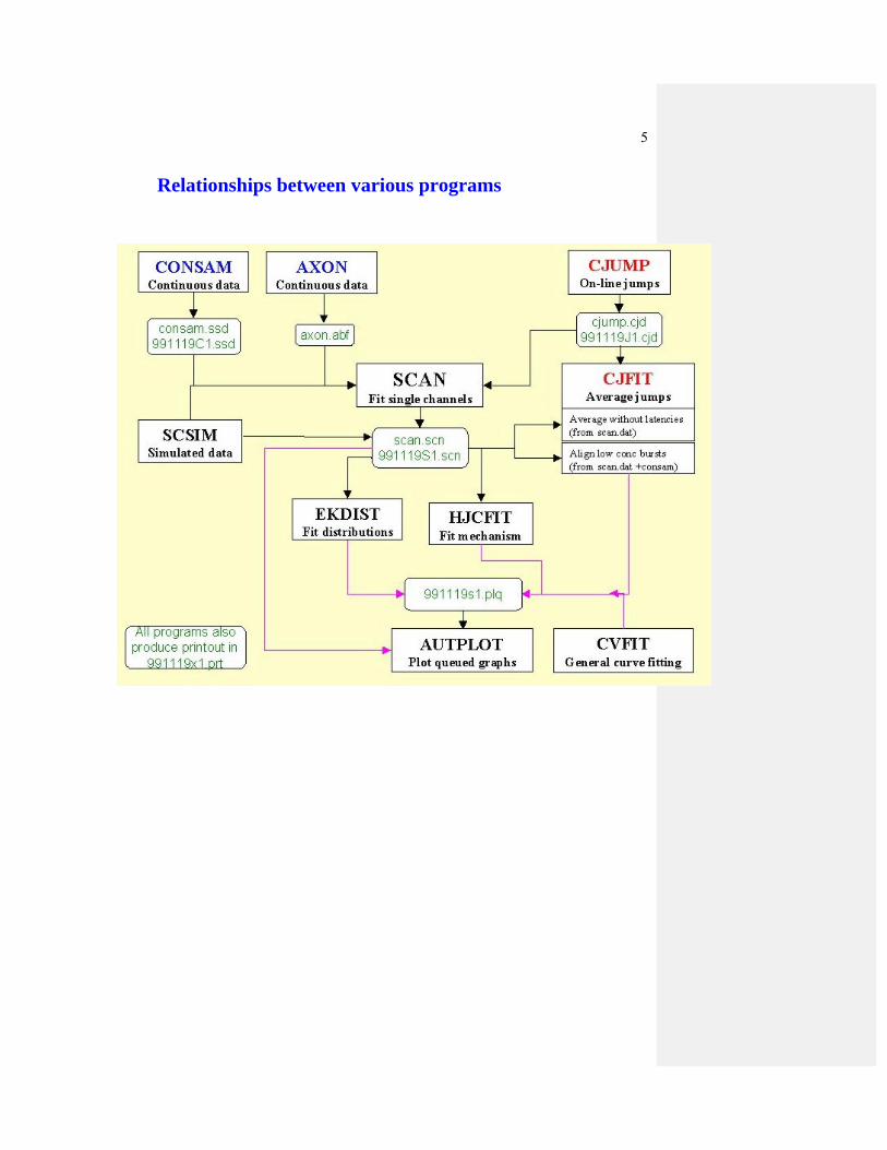
The meaning of these quantities can be illustrated by simulation. Suppose we have an experiment like that illustrated in Fig 1A. The true curve is a Langmuir hyperbola with Ymax = 1 and K = 1, and five concentrations are used, from 0.1K to 10K. The errors on the points are constant, s(y) = 0.1. We now simulate 10000 experiments, with random errors added to each of the points shown in Fig 1A, the errors having a Gaussian distribution, with a standard deviation of 0.1. Each of the 10000 ‘experiments’ is then fitted with a Hill equation (e.g. using eq. 3 in CVFIT –see list of equations). The fits produce 10000 estimates of K, 10000 estimates of Ymax, and 10000 estimates of the Hill coefficient, nH, which should, of course, be 1 in this case. The distributions of the 10000 estimates found in this way are shown in Figs 1B, 1C and 1D respectively. It can be seen that the estimates of Ymax are not too bad in most experiments, despite the fact that the points do not get as near to a plateau as would be desirable, but there is a long tail of Ymax estimates that are much too high. The values for K and nH show a considerable scatter, some values being far too large. None of the distributions is symmetrical, and that is why the (symmetrical) error limits give by citing a standard deviation are rather crude. Likelihood intervals (see below) cater for this asymmetry.

33

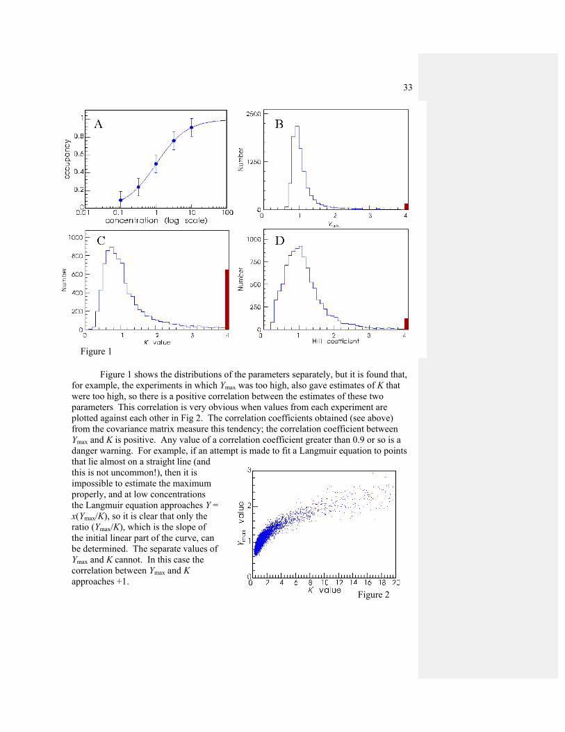
Figure 1 shows the distributions of the parameters separately, but it is found that,

for example, the experiments in which Ymax was too high, also gave estimates of K that were too high, so there is a positive correlation between the estimates of these two parameters This correlation is very obvious when values from each experiment are plotted against each other in Fig 2. The correlation coefficients obtained (see above) from the covariance matrix measure this tendency; the correlation coefficient between Ymax and K is positive. Any value of a correlation coefficient greater than 0.9 or so is a danger warning. For example, if an attempt is made to fit a Langmuir equation to points that lie almost on a straight line (and this is not uncommon!), then it is impossible to estimate the maximum properly, and at low concentrations the Langmuir equation approaches Y = x(Ymax/K), so it is clear that only the ratio (Ymax/K), which is the slope of the initial linear part of the curve, can be determined. The separate values of Ymax and K cannot. In this case the correlation between Ymax and K approaches +1.

Figure 1

Figure 2

34

The use of a standard deviation implies that the error limits are symmetrical (i.e. can be expressed as the best estimate plus or minus some fixed value). These standard deviations are helpful only insofar as the likelihood surface has a quadratic (and therefore symmetrical) shape near its maximum. This is frequently not the case for non-linear problems. For example if you are trying to estimate a maximum Popen value which is close to 1.0, the upper error limit can obviously not exceed one, though the lower limit may be quite low. For example, if the best estimate of the parameter was 0.95, the approximate standard method might produce a standard deviation of 0.15 giving limits (± 1 SD) as 0.8 to 1.1, which is meaningless! For the same data the corresponding Likelihood interval might be 0.7 to 0.98, which makes more sense. In other cases, where a parameter is not well-defined, the 'standard deviations' may be highly unreliable, but calculation of likelihood intervals may reveal that a sensible lower limit can be found even though the upper limit is undefined (essentially infinite). Practical examples of such calculations are given by Colquhoun & Ogden (1988, Journal of Physiology, 395, 131-159). Calculation of likelihood After the fit, the minimum in the sum of squared deviations, Smin, is printed. If the further assumption is made that the errors in y (at a given x) have a Gaussian distribution, then this can be converted into a likelihood, and the fitting process is, with this assumption, a maximum likelihood fit. The corresponding value of the maximum log(likelihood) is also printed after the fit (the way in which this was calculated was corrected 11-May-2001 for the case where weights are set to 1 and errors are estimated form residuals). The likelihood of the observations, for Gaussian errors, is

∏= ⎥

⎥⎦

⎤

⎢⎢⎣

⎡⎟⎟⎠

⎞⎜⎜⎝

⎛ −−n

i i

ii

i

y1

2

2

2)(

exp2

1σ

μπσ

The log(likelihood), needed for doing a likelihood ratio test to compare two fits, is therefore

∑∑==

⎟⎟⎠

⎞⎜⎜⎝

⎛ −−⎟

⎟⎠

⎞⎜⎜⎝

⎛=

n

i i

iin

i i

YyL

12

2

1max 2

)ˆ(2

1lnσπσ

For comparison of fits of two different (nested) model to the same data, this value can be used for a likelihood ratio test. (Nested means that one equation is a special case of the other, e.g. 2 versus 1 Langmuirean components.). In general, my own feeling is that such tests are not very useful (see p.546 in Colquhoun, D. & Sigworth, F. J. (1995). Analysis of single ion channel data. In Single channel recording, Sakmann, B. & Neher, E., pp. 483-587, Plenum Press, New York). In the case where the weights are set to 1 and the error variance is estimated from residuals (weighting method 1), then if we use the (biassed) maximum likelihood estimate of σ2, namely sres

2 = Smin/n, the maximum log(likelihood) becomes

35

( )1)π2ln(2

2resmax +−= snL

The log-likelihood ratio is found as the difference between the values of this quantity for the two fits, and twice this value is distributed approximately as χ2 with a number of degrees of freedom equal to 2 (the difference between the number of free parameters in the two fits). Calculation of Likelihood intervals.

If you ask for this calculation, then first specify the value of m for m-unit likelihood intervals. A value of m = 0.5 corresponds roughly to (± 1 SD limits, and m = 2.0 corresponds roughly to ± 2 SD limits (see Colquhoun & Sigworth, 1995). Next specify which parameters to calculate them for (it is simpler to ask for one parameter at a time). Then you are asked if you want to calculate a lower limit, an upper limit or both. The calculation is done by a bisection method, using a minimisation at each iteration with the parameter in question fixed, until the parameter value that makes the maximum log-likelihood m units below the value for the best estimate is found. This may be slow with complicated functions or large amounts of data, but for the typical CVFIT problem it does not take long. At the end of each calculation the calculated limits is printed. As a check the maximum log-likelihood for the original fit (Lmax) is printed, together with the value m units lower (Lcrit = Lmax - m); if the calculation has been successful the log-likelihood corresponding to the calculated limit, Llimit , should be very close to its target value, Lcrit.

Calculation of each limit needs a pair of initial guesses that bracket the value for the lower limit. For example if the best estimate of a parameter was 5.2 with approximate SD of 0.5, then to calculate the lower m=0.5 unit limit the upper guess must be safe if you give 5.2, and the lower guess will be safe if you make it substantially lower than 5.2 - 0.5 = 4.7; say 4.0 or even 2.0. The present version supplies these initial guesses for you, and in ‘clean’ cases the values for the limits will simply be printed out. Given that one tends to want likelihood intervals in ‘difficult’ cases, in which parameters are not well determined, you may not be so lucky. If the automatic guesses do not appear to contain the result you will get asked to supply different guesses, and if no guesses seem to contain the result then that limit may be infinite. It is also possible that some of the minimisations may not converge, in which case Llimit may appear to change erratically with the value used for the limit. It is worth noting that a strong argument can be made for the view that the best method of assessing the certainty of a parameter value is neither to use SDs nor likelihood intervals, but is to do as many separate experiments as possible. If each experiment can provide a value of the parameter, then it is simple to see how consistent the values are.

36

List of equations that are available in CVFIT (Feb 1998) (Warning –some of these options have not been used for a long time –they stem from the original PDP 11-40 version. Let me know if they don’t work any longer!) Equation (1) Polynomial equation In general the polynomial of degree n is

in

ii xaYxY ∑

=

+=1

)0()(

In the program, the parameters appear as Y(0), a1, a2 etc Special cases include (a) straight line (degree 1), with intercept Y(0) and slope a1,

Y = Y(0) + a1x (b) quadratic

Y = Y(0) + a1x + a2x2 , and so on. Sub-options You can fit a disjoint polynomial, i.e. on that has degree n1, say, below a specified x value, but a different degree above that x value. For example the empirical description of a current-voltage relationship can sometimes require a straight line below a certain voltage but a quadratic or cubic above that voltage. The Schild plot option If you specify a straight line, then you are offered the option to fit the Schild equation

B

1KxY +=

where Y the dose ratio, x is the antagonist concentration, and KB is the equilibrium constant for antagonist binding (it is the only free parameter in this case, because the slope is unity in the Schild equation). (There is also an option that allows you to do this if you entered dose ratio − 1, rather than dose ratio). The advantage of this option is that the error calculations give errors for KB itself, rather than its reciprocal which is what a regular straight line fit would give.

N.B. you enter as data the concentrations and dose-ratios not their logarithms (see notes above on Log scales and other transformations).

Common X intercept for a set of lines.

When fit mode 3 is used (see above), a set of lines can be constrained such that they all have the same intercept on the X axis (this was designed to fit a set of current-voltage curves with a common reversal potential). In this case the free parameters are a separate slope for each line, plus the common intercept.

Equations (2) Langmuir equation, and (3) Hill equation

37

These will be discussed together, since the former is a special case of the latter in which the Hill slope, nH, is fixed to 1. The Langmuir and Hill plot fits now have many options, as follows. Any number (m say, see below) of Langmuir/Hill components can be fitted to each set (curve) now. The equation fitted is as follows. Define Y(x) as the sum of m Hill-equation components

∑= +

+=k

rn

r

nrr

KxKxY

YxY1

max

H

H

)/(1)/(

)0()(

where x is usually the concentration of some ligand. The K values are not in general real equilibrium constants, and should usually be denoted EC50, rather than K. This increases with x from the baseline value Y(0) at zero concentration, to a total amplitude of Y(0) + ΣYmax (usually Y(0) will be fixed to 0, but it can be estimated if necessary). There is also an option to fit a decreasing Hill/Langmuir curve which falls from Y(∞) + ΣYmax at zero concentration to a baseline value of Y(∞) at high concentration. Commonly Y(∞) will be fixed at 0, but in some cases it should be estimated as a free parameter.

∑= +

+∞=k

rn

r

r

KxYYxY

1

max

H)/(1)()(

In the program the parameters appear as Y(0) or Y(inf), and Ymax1, Ymax2, K1, K2, nH1, nH2 etc (for the first and 2nd components in each curve). If several sets are being fitted simultaneously (fit mode = 3) you are asked whether you want to estimate all the parameters, or to have some in common for all sets. (a) a common Ymax value for all sets, but separate K values for each set (b) a common K value for all sets, but separate Ymax values for each set (c) as (b) but fitting to the log(y) values, as described next. This is available only if there is one component (m = 1) only is fitted and the baseline value is zero. (d) When two components are fitted to each curve (m = 2), another option appears, to fit the EC50s (K values) and maxima separately to each curve, but to have the fraction of the total amplitude that is accounted for by the first component as a common parameter between all curves, i.e. p = Ymax1/(Ymax1 + Ymax2)is treated as a parameter that is common to all curves. The log(y) fit for Hill equations. It is often the case that smaller values of y have smaller standard deviations. If there are not good estimates of the standard deviations then this sort of weighting may be achieved by using weighting option 4 (see above) to give a constant coefficient of variation to each y value. This may, for example be done with option (b) above (common K value for all sets, but separate Ymax values). However, a similar effect can be obtained by doing the fit with log(Yij) values (equally weighted, implying constant coefficient of variation in Yij themselves). If each curve has only one component then, although the response is non-linearly related to K and nH (requiring an iterative procedure), log(Yij) is linearly related to log(Yj

max). This means that only K and nH need to be estimated iteratively (by Simplex), and, at each stage the k values of Yj

max (one for each set) can be

38

calculated explicitly from the current values of K and nH. Writing down the least squares equations shows that they can be found from

log( ){log( ) log[ ( / ) ]}

maxYy x K

nji

n

ij ijn

j

j

=

+ +=∑

11

where yij is the observed response for ith concentration in the jth set. This is a rather nice mixed linear/non linear procedure. It is very fast, but for any normal number of data points this does not matter any more, now that computers are so fast. Equation (4): Langmuir hyperbola(s)+ straight line This is a sum of Langmuir components + a linear component, slope*x. This is actually a sub-option of eq.2, with the addition of one value of the parameter slope for each set fitted. It was designed for fitting results of binding experiments in which ‘non-specific’ binding is fitted as a linear component (as In Paton & Rang, 1966). Equation (5): Hill equation(s) + straight line Same as (4), but Hill rather than Langmuir equations. Equation (6): Power function It is not uncommon to determine only the lower end of the dose-response curves, when doing a Schild analysis. Without maxima, it is not possible to fit Hill equations etc to the curves, but we often find that the low-concentration limit of the Hill equation is quite adequate. This is a power function (y = axn), which corresponds to a straight line in log-log coordinates. There are all sorts of ways in which this could be parametrised, but the one used in CVFIT is

n

xxyy ⎟⎟

⎠

⎞⎜⎜⎝

⎛=

0

.

The two free parameters are n and x0, the latter being the value of x when y = y , and y is the mean of all your y values, which is a constant determined by your data. It is not essential to include the scaling constant y ; the reason for formulating it in this way is to make it easier to provide initial guesses for the value of x0, which is needed for fitting (though the current version of CVFIT does the guesses for you so you will only have to provide them manually if the automatically generated guess is bad). Since y is roughly at the midpoint of your data, it is easy to eyeball the corresponding value of x. The value used for y appears along with the fitted parameters, and, on the print out, the result is also expressed in its logarithmic form

)(log)(log 1010 xnay += , where

39

)(log)(log 01010 xnya −= , and n is the slope of the log-log plot. Equation (7): Equilibrium binding inhibition curves (Langmuir) This is designed for experiments in which equilibrium binding of a labelled ligand (y) is plotted against inhibitor concentration (x). A single decreasing Langmuir curve is fitted, but instead of fitting the IC50 (as eq.2 would do) would, the fitted parameter is KB, the equilibrium constant for binding of the antagonist. The equation for this sort of experiment is that for competitive inhibition, viz.

BA

A

/11)0()(

KxccYYY

+++

+∞= ,

where cA is the normalised concentration of the labelled ligand (its concentration divided by its equilibrium constant). Values for cA are given as the set variable when data are entered. The asymptote, at high inhibitor concentration, Y(∞), may be fixed at zero if appropriate. By fitting the correct equation we obtain errors for KB directly, and we avoid the so-called Cheng-Prusoff correction (which is, of course, only a correction for having fitted the wrong equation). Equation (8): Exponential binding onset curves Designed to fit exponential onset of binding.

])(exp[)( 11max xkckYtY −+ +−= , where x is time, and the ligand concentration for each data set, c is specified as the ste variable when data are entered. The association rate constant, k+1, and the dissociation rate constant, k-1, are denoted ak1 and ak2 in the program. There are two options –the zero-time value, Ymax, may be common to all data sets, or estimated separately for each set. Equation (9): General exponential and geometric curves The exponential option fits a general sum of n exponential terms, with amplitude ai and time constant τi for the ith component, thus

∑=

τ−+∞=n

iii xaYxY

1)/exp()()( ,

where x is usually time, and the parameters Y(∞), ai and τI are denoted in the program as Y(inf), amp1, amp2 etc, and tau1, tau2 etc. The geometric option fits a sum of n geometrically-decaying time constants, in which the place of the time constant is taken by the ‘mean’ for each component μI’ The equation is

Y x Y aii

x

i

n( ) ( )= ∞ + −

⎛⎝⎜

⎞⎠⎟

=∑ 1

1

1 μ,

where μi is referred to in the program as ‘tau1’, ‘tau2’ etc.

40

Equations for equilibrium Popen curves These are listed on the (green) submenu, above. The mechanisms listed all involve binding of two agonist molecules (apart from 24 and 25 which are general for n molecules). No singly-liganded binding is included, but all the options include the possibility of channel block by the agonist iteslef.. The case where the two binding sites are equivalent can be represented, for mechanisms (10) to (17) as

Note: throughout this section, the ‘efficacy’ or ‘gating constant’, denoted E, is defined as opening rate divided by shutting rate. For concentration-response curves and arbitrary maximum response, Ymax, can be fitted, but for genuine Popen versus concentration curves, Ymax should be fixed to 1.0. For mechanisms (10) and (12), the following equation is fitted (with K1 = K2 for the former).

⎥⎦

⎤⎢⎣

⎡⎟⎟⎠

⎞⎜⎜⎝

⎛++++

=

B2

21

2

1

21

2

2

1121max

KxE

KKx

Kx

KKxE

Yy

where x is agonist concentration. When the sites are not equivalent

⎥⎦

⎤⎢⎣

⎡⎟⎟⎠

⎞⎜⎜⎝

⎛+++++

=

B2

21

2

21

21

2

2

111max

KxE

KKx

Kx

Kx

KKxE

Yy

41

Mechanisms (11), (13) and (17) ask you to specify a single channel burst length, which is used to constrain the parameters (to be used for real Popen curves only). Mechanism 15 Two independent del Castillo-Katz subunits This refers to a receptor with two independent subunits each of which can bind one agonist molecule, and bot of which must be in the AR* state for the channel to open

Mechanisms 16 and 17: Non-equivalent subunits The case where the two binding sites are not equivalent can be represented as

In this scheme the two binding sites may be different and Kij represents the equilibrium constant for binding to the ith binding site (subunit), with j = 1 for the first binding (other site vacant) and j = 2 for the second binding (other site occupied). Microscopic reversibility dictates that

21122211 KKKK = . The parameters for the fit are chosen as K11 and ‘non-eq’ = K12/ K22 = K11/ K21 , and ‘coop’ = K11/ K12 = K21/ K22 , (the two forms for each follow from the microscopic reversibility constraint). After the fit the values of all four equilibrium constants are printed out. The expression that is fitted for this mechanism is

42

⎥⎦

⎤⎢⎣

⎡⎟⎟⎠

⎞⎜⎜⎝

⎛+++++

=

B2

2211

2

2111

2211

2

2

111max

KxE

KKx

Kx

Kx

KKxE

Yy .

Mechanism 24 and 25 are general, for binding of n agonist molecules Mechanism 24 Sequential binding of n molecules followed by opening

If we have n binding steps, followed by a single activation step from the fully-liganded state (with equilibrium constant En), the argument is very like that for the Adair equation, except that there is now one more state, the active state, which gives rise to the last term on the top and bottom lines. The equilibrium fraction in the active state is

pE

K

B n rK

EK

n

n

nr

rn

n

nr

nact

A]

A] A]( )

[

( , ) [ [∞ =

+ +=

∑11

where we define

K Kr ii

r=

=∏

1

so K K K K K K K2 1 2 3 1 2 3= =, etc. These quantities have units of (M)r , and the rth roots are the geometric means of the K values. This makes sense because it is equivalent to averaging log(K) values, i.e. to averaging free energies. Similarly the equilibrium fraction of sites that are occupied is

43

pB n r

KE

K

B n rK

EK

r

rn

n

nr

n

r

rn

n

nr

nocc

A] A]

A] A]( )

( , ) [ [

( , ) [ [∞ =

− − +

+ +

=

=

∑

∑

1 1

1

1

1

As in the Adair case (section 1.4), analytical expressions for the EC50 and BC50 are possible only for n <4. The Hill slope for the active state, pact(∞), is, in general,

nn n r B n r

K

B n rK

r

rr

n

r

rr

nH

A]

A]=

+ −

+

=

−

=

−

∑

∑

( ) ( , ) [

( , ) [1

1

1

11

.

Notice that this does not depend either on En or on Kn. The Hill slope, nH, for the binding curve can also be written explicitly for any n, but the expression is too long to include here. Mechanism 25 Monod-Wyman-Changeux mechanism with n subunits A mechanism with only two conformations can be written, for the general case of n binding site. This scheme represents the MWC mechanism, if we suppose, in addition, that the affinity is the same for all receptors in the inactive conformation, so K1 = K2= K3 = ..... = Kn (= K say), and that that the affinity is the same for all receptors in the active conformation, so K1* = K2* = K3* = ..... = Kn* (= K* say).

The equilibrium constant for binding to a site on the inactive conformation (R) is denoted K, and for binding to a site on the active conformation (R*) is denoted K*; according to the MWC assumption these are the same regardless of how many ligands are already bound, so no subscript is needed.

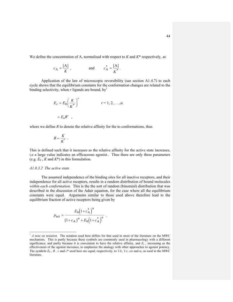
44

We define the concentration of A, normalised with respect to K and K* respectively, as

cKAA

=[ ] , and c

KA* A

=[ ]

* .

Application of the law of microscopic reversibility (see section A1.4.7) to each cycle shows that the equilibrium constants for the conformation changes are related to the binding selectivity, when r ligands are bound, by1

E E KK

r

r=

⎛⎝⎜

⎞⎠⎟0 * r = 1, 2, . . .,n.

= E Rr

0 , where we define R to denote the relative affinity for the to conformations, thus

R KK

= * .

This is defined such that it increases as the relative affinity for the active state increases, i.e a large value indicates an efficaceous agonist.. Thus there are only three parameters (e.g. E0 , K and K*) in this formulation. A1.8.3.2 The active state The assumed independence of the binding sites for all inactive receptors, and their independence for all active receptors, results in a random distribution of bound molecules within each conformation. This is the the sort of random (binomial) distribution that was described in the discussion of the Adair equation, for the case where all the equilibrium constants were equal. Arguments similar to those used above therefore lead to the equilibrium fraction of active receptors being given by

( )

( ) ( )p

E c

c E c

n

n nactA

A A

=+

+ + +

0

0

1

1 1

*

* .

1 A note on notation. The notation used here differs for that used in most of the literature on the MWC mechanism. This is partly because these symbols are commonly used in pharmacology with a different significance, and partly because it is convenient to have the relative affinity, and Er , increasing as the effectiveness of the agonist increases, to emphasize the analogy with other approaches to agonist potency. The symbols E0 , R , c and c* used here are equal, respectively, to 1/L, 1/c, cα and α, as used in the MWC literature.

45

This, multiplied by a maximum response, Ymax, is what is fitted by CVFIT. For genuine Popen curves, fix Ymax to 1.0.

46

Notes on fitting the Schild equation with CVFIT

(1) The case of full dose-response curves

When the dose-response curves all have well-defined maxima, the best procedure is to pool the curves after normalising them to the same maximum response. The normalisation can be done as follows.

(a) Fitting the curves separately (fit mode 2) with some suitable equation (often the Hill equation will suffice). (b) Accept the option to normalise with respect to the fitted maxima (c) Re-fit the set of normalised dose-response curves with the same equation, using either fit-mode 4 to get dose-ratios, or, probably better, fit-mode 5 to fit the Schild equation directly to the set of dose-response curves. The latter procedure is illustrated in the Summer Course notes, and amounts to constraining the fitted curves to have the spacing defined by the Schild equation (as well as constraining them to be parallel). The result will, of course, correspond to an exactly straight Schild plot with a slope of 1. With this approach there is no need to do Schild plot at all, though it is probably sensible to do it anyway.

(2) The case where the dose-response curves have no well-defined maximum

If the dose-response curves have not got well defined maxima, but have an x value (agonist concentration) in common, you can use the option in CVFIT to normalise with respect to the response at a particular agonist concentration, and then proceed as above. However, good Schild data are unlikely to have such a common agonist concentration, so the following procedure will be better.

If the dose-response curves cannot safely be averaged, the Schild plot should be used.

(a) Each set of dose response curves should be fitted separately for estimation of dose-ratios, using fit mode 4. When only low agonist concentrations are used, the low-concentration limit of the Hill equation (the power function, equation 23) will often be a suitable thing to fit (see below for notes on the power function).

(b) Average the dose ratios for all experiments and calculate the standard deviation of this mean (the so-called “standard error”). Enter into CVFIT the mean dose ratio − 1 as the y value, antagonist concentration as the x value, and the standard deviation of the mean (smoothed if necessary) in the SD column, to be used for weighting the fit (NB do not take their logs before entering -the SD you have is for the non-logged value).

(c) Display the averaged (dose ratio − 1) data in log-log coordinates and fit with the power function (eq. 23). This is a straight line with a slope of n in log-log coordinates. Thus n is the slope of the Schild plot. Judge whether the line is sufficiently

47

straight, and (from the estimate of n and its standard deviation) whether the slope is sufficiently close to 1 for you to believe that the Schild equation is valid.

(d) If you decide that the Schild equation is valid, then re-fit the (dose ratio − 1) with the Schild equation for estimation of the antagonist equilibrium constant, KB. This means fitting with a straight line that has a slope fixed at 1. A new option in CVFIT allows this to be done conveniently. If you choose eq. 1 (polynomial fit) with degree=1 (i.e. a straight line) you now get offered the option to fit the Schild equation to the original data (not in logged form). Choose this option and do a weighted fit; this fits a line to

y = (dose ratio − 1) = [B]/ KB. There is only one free parameter, KB, so you can get estimates of error directly for the fitted KB value, as the usual approximate standard deviation, and/or as likelihood intervals for KB. Notes on the power function (eq, 23) It is not uncommon to determine only the lower end of the dose-response curves, when doing a Schild analysis. Without maxima, it is not possible to fit Hill equations etc to the curves, and we often find that the low-concentration limit of the Hill equation is quite adequate. This is a power function which corresponds to a straight line in log-log coordinates. There are all sorts of ways in which this could be parametrised, but the one used in CVFIT is

n

xxyy ⎟⎟

⎠

⎞⎜⎜⎝

⎛=

0

.

The two free parameters are n and x0, the latter being the value of x when y = y , and y is the mean of all your y values, which is a constant determined by your data. It is not essential to include the scaling constant y ; the reason for formulating it in this way is to make it easier to provide initial guesses for the value of x0, which is needed for fitting (though the current version of CVFIT does the guesses for you so you will only have to provide them manually if the automatically generated guess is bad). Since y is roughly at the midpoint of your data, it is easy to eyeball the corresponding value of x. The value used for y appears along with the fitted parameters, and, on the print out, the result is also expressed in its logarithmic form

)(log)(log 1010 xnay += ,

where )(log)(log 01010 xnya −= .

DC 18-Aug-97

49

Help notes for SCAN

Single channel time-course fitting for PC Some general notes about keyboard input Numerical input. All input is read in ASCII form so that it is not essential, for example, to have a decimal point in floating point numbers (as it is in basic Fortran). Thus 200, 200., 200.00, 2e2, 2.e2 are all acceptable inputs for the floating point number 200. If asked for two (occasionally 3) numbers at once, as for example ‘Xmin, Xmax = ‘, then enter two numbers separated by a comma. Most (but not all) inputs have a default (in square brackets) and hitting enter with typeing anything gives this default value. When 2 numbers are input, and the default is OK for one but not the other, then only the one to be changed need be entered, e.g. in response to ‘Xmin, Xmax [0,10] = ‘, typing only ‘1’ gives Xmin=1., Xmax=10., and typing only ‘,20’ (with comma before 20) would give Xmin = 0., Xmax = 20. Usually the numlock key switches itself on so you can use numerical keypad. Yes/No input. Type ‘Y’ or ‘N’ in response (upper or lower case). Again there is usually a default, as, in ‘Try again [Y] ?’. Hitting enter gives the default and hitting INS key gives the opposite of the default (so rarely necessary to use the ‘y’ or ‘n’ keys). Usually the numlock key switches itself on so you can use numerical keypad. New data structure: files used by SCAN (Jan 1999) The progressive demise of the floppy disk has made the original data structure no longer ideal. In particular, the idea of keeping a summary of many analyses on a scandat.dat floppy disk has become rather clumsy, for the purposes of record keeping. Now that we always keep the scantemp.dat file (which was originally designed to be temporary) space is actually wasted because scantemp.dat contains everything that is in an experiment file on you scandat.dat floppy (as well as much else). It is proposed now to keep only a (modified version of) scantemp.dat, and this will be referred to generically as a SCAN.SCN (or SCAN.DAT) file. This is a single file, one is generated each time a run of SCAN is completed (there will no longer be several analyses on one scandat.dat file). Default suffices, as below, have been incorporated into program defaults (May 2000) to

reduce possible ambiguities that result from having different sorts of file that end in .DAT.

Default file names

The identification of files will be aided if they are named according to the date on

whicj the experiment was done (not the date it was analysed). If we restrict the file names to

8 characters then the following system is suggested, for an experiment that was done on 16-

Oct-96. The US date order, 96-10-16, makes sense, so that when files are sorted ‘by name’,

experiments will appear in chronological order.

50

961016cs.SSD (previously 961016cs.DAT) for CONSAM file 961016cs.PRT for CONSAM printout 961016cj.CJD (previously 961016cs.DAT) for output of data from CJUMP5 961016cj.PRT for CJUMP5 printout 961016sc.PRT for SCAN printout 961016sc.PLQ for SCAN plot queue 961016sc.SCN (previously 961016sc.DAT) for output from SCAN It might be useful also to distinguish whether the output is from analysis of a steady state record (e.g. 961016ss.SCN ) or from analysis of single channel after a jump (e.g. 961016cj.SCN) 961016ek.PRT for EKDIST printout 961016ek.PLQ for EKDIST plot queue (or put all plots into 961016sc.PLQ) The only way to distinguish different patches on the same date is to insert another number. This can be done with one digit if you have up to analysable 10 patches on the same day. The present default file name therefore uses only one letter to distinguish which program the file originates from (C=CONSAM; J= CJUMP; S=SCAN and E= EKDIST, with the patch number after it. Use of the default suffices now (May 2000) suggested, also clarifies which program a file came from Thus we have, for patch number n, on 16-Oct-96,

961016Cn.DAT for CONSAM file (n = 0, . . 9) 961016Cn.PRT for CONSAM printout (n = 0, . . 9) 961016Jn.CJD for output of data from CJUMP5 961016Jn.PRT for CJUMP5 printout 961016Sn.PRT for SCAN printout (n = 0, . . 9) 961016Sn.PLQ for SCAN plot queue (n = 0, . . 9) 961016Sn.DAT for SCAN results (a SCAN.DAT file, the input for EKDIST) 961016En.PRT for EKDIST printout (n = 0, . . 9) 961016En.PLQ for EKDIST plot queue (or put all plots into 961016Sn.PLQ) 961016Hn.PRT for HJCFIT printout (n = 0, . . 9) If a single patch record is split up into several consam files (e.g. because it is so long that you have not got enough disk space to hold a single 300 Mb consam), then it will be necessary to change the suffix too. For example if patch number two on 16-Oct-96 was digitised in two parts, the two consam files would be named 961016C2.DA1 and 961016C2.DA2, with analagous .suffices for the other files.

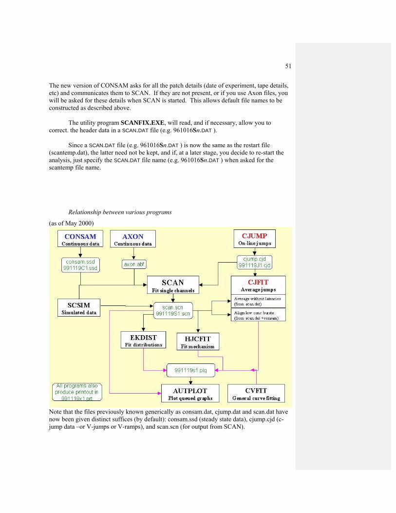
51

The new version of CONSAM asks for all the patch details (date of experiment, tape details, etc) and communicates them to SCAN. If they are not present, or if you use Axon files, you will be asked for these details when SCAN is started. This allows default file names to be constructed as described above. The utility program SCANFIX.EXE, will read, and if necessary, allow you to correct. the header data in a SCAN.DAT file (e.g. 961016Sn.DAT ). Since a SCAN.DAT file (e.g. 961016Sn.DAT ) is now the same as the restart file (scantemp.dat), the latter need not be kept, and if, at a later stage, you decide to re-start the analysis, just specify the SCAN.DAT file name (e.g. 961016Sn.DAT ) when asked for the scantemp file name.

Relationship between various programs

(as of May 2000)

Note that the files previously known generically as consam.dat, cjump.dat and scan.dat have now been given distinct suffices (by default): consam.ssd (steady state data), cjump.cjd (c-jump data –or V-jumps or V-ramps), and scan.scn (for output from SCAN).

52

Old data structure: files used by SCAN SCAN.INI: keeps values of the settings used for the last analysis SCANTEMP.DAT: this file stores the whole current state of the analysis, including the position of every transition in the data. It is what is used to re-start an analysis where you left of, after leaving SCAN, and it is what is written automatically to the hard disk (as often as specified in the blue parameter menu). It can also be written at any time using the More Options menu. Originally this was intended as a temporary file, but now increased disk and network capacity means that it has become feasible to keep this file, and the original CONSAM file. When this is done it is possible to go back to any specified opening in the record at any time. SCANDAT.DAT. This is the main summary of the output from SCAN, and it is what is read by EKDIST for the fitting of distributions. It contains all the open times, shut times and amplitudes (but not their exact position in CONSAM, or the baseline positions). It is designed to fit on a 3.5” floppy disk, for easy backup. RSCAN.BAT: a little file to be run by Windows to run SCAN. Using this ensures that any error messages are visible if there is a crash. SCAN.ICO: an icon for WINDOWS EKDIST.TMP: a file output automatically by EKDIST when transition sequences are listed. (in the root segment, C:\, not the directory where the program is run). I is kept in the root segment, C:\, not in the directory where the program is run. When it is present an item, show ekdist data, appears on the SCAN goto pop-up menu which allows you to view in the original data any of the transition sequences listed by SCAN Getting started. The program starts with the usual ‘blue window’, to specify how you want to keep the print-out on disk, for printing later (see separate notes for details). Restarting. The next question asks whether you wish to restart SCAN. Details of the run are written to disk automatically after every n transitions (n is set in the parameter window, see below). Also whenever you leave SCAN, details are kept on the disk (whether or not you ask for data to be written to permanent file). These details are kept in a file (SCANTEMP.DAT, in same directory as program), and they allow the program to be restarted at the point where it was left (or from where it was at the time of the last automatic disk-write if the program crashes). If you say that you wish to restart, you are asked whether you want to ‘go straight to write permanent data file?’. Say yes only if the object of restarting was to make a permanent data disk; otherwise the data will appear on the screen showing the last fitting that was done (marked with vertical yellow arrow), and you can carry on fitting as usual. Normal start. First say where the data are. There are various options, but the values are always expected to be 16 bit integers, and to be continuously sampled to disc with no breaks.

Our standard sampling program CONSAM produces such a file, CONSAM.DAT, with a header that contains information such as sampling rate and filter cut off frequency.

There are also options to read data from AXON INSTRUMENTS (e.g. pClamp) files, from PDP CONSAM files and from any unspecified 16-bit integer data file (as long as you can specify where the data start, i.e. the length of any header that the file may have).

53

To use the Axon (pClamp) option, the data file must be an Axon Binary format (.ABF) file, sampled with no gaps (operationmode=3), with 16-bit integer data (dataformat=0), sample on one channel only (inchan=1). It should work for either Digidata 1200 or the older Labmaster/TL-1. Note that the display is scaled so that full-scale is the whole dynamic range of the ADC converter to encourage use of the full range. If you have not done so then set a display gain factor greater than the default value of 1.0 (see below).

Note that these continuous data files can be plotted out with multiple lines per page, whenever you are in the graph drawing subroutine VPLOT. e.g. in AUTPLOT or CVFIT or any other program that draws graphs (rather than histograms), by going to ‘.: MORE OPTIONS’ and then ‘/: MULTIPLE TRACE’ –see VPLOTHLP.DOC for more details. There is now also a stand-alone program, PLOTSAMP.EXE which will plot these files without having to run AUTPLOT etc.

Specify the path and name for the data file (e.g. CONSAM.DAT) that contains the digitised single channel record. Then specify which step-response function is to be used, by specifying the set-up, and filter setting, appropriate for your data. When this has been done, a large blue window appears containing the default parameter values. This works rather like a spreadsheet; you can move up and down with the arrow (cursor) keys, or with TAB/ SHIFT-TAB. When F1 is hit, a help box appears that explains the meaning of the current parameter. Each entry can be edited (see help box); the space bar toggles the Y(es)/ N(o) entries, and new numerical values can be typed in. When all the values are as required, then hit enter or esc to continue. Further notes on default parameters. The blue parameter window

This appears when SCAN is first started, and can be changed at any time after fitting has started, via ‘.: MORE OPTIONS’, and ‘NEW PARAMETERS’

Various values that are essential for the proper function of the program are set here. Some values concern matters like the display and array sizes, and these will rarely need to be changed. The most important values set here are those that control the sensitivity and other behaviour of the automatic search for an initial guess for fitting, as used by FIT-AUTO. These will usually need to be tailored for the sort of record that you are fitting, in order to reduce the number of times that manual intervention is needed to get the fit you want. The aim is to tailor the fitting parameters so that FIT (AUTO) works as reliably as possible.

Each line has a brief description which appears when F1 is hit. The individual items are as follows.

First page • 1. Invert trace. Openings must appear as downward deflections on screen. Set to

‘yes’ of the digitised data has openings upwards [NB can be set only at start of a new analysis].

• 2. Auto-fit to avoid sublevels if possible. Set to Yes if you want an attempt to be made to fit open-shut-open, rather than a sublevel. If two transitions in the same direction are ‘close’ (see below) together, then if this parameter is set to No a sublevel is fitted, but if it is set to Yes, then the program looks at the first derivative

54

of the trace in an attempt to find a guess for the positions of a rapid open-shut-open sequence on the opening phase (or shut-open-shut on the shutting phase). Sensitivity controlled by parameter 19.

• 3. Percent of full amplitude for critical level/or Multiple of RMS noise for critical level. The threshold level used by the program when searching for transitions, to get the initial guess for fitting. This can be expressed as a percentage of the rough ‘full amplitude’ which is set when SCAN is started (usually 12-18% is OK), or it can be expressed as a multiple of the RMS baseline noise (set via parameter 31 below or via pop-up ‘new sensitivity’ menu (more options/3)).

• 4. Number of points past critical level. The number of data points that must pass the level set by the previous parameter for a transition to be deemed to have occurred (1 to 3 usually).

• 5. Number of shut points to be fitted at ends. the number of baseline (shut) points to be included at each end of the fitting of an opening (these are used to estimate amplitude, and the final fitted baseline is used to re-adjust the display so that the baseline is set at a fixed place (see Display baseline) on the screen. (40 points is usually reasonable)

• 6. Minimum number of shut points for baseline. During the fitting, any piece of baseline with more points than the number specified here is used to estimate the amplitude of the opening(s) adjacent to it. These points are initially shown in blue after the fit. (10 points is usually reasonable)

• 7. Initial display expansion factor. Factor by which display is expanded when Expand is first hit.

• 8. Auto-write to disc every nth transition. The results are written automatically to SCANTEMP.DAT every nth transition. This is partly to guard against loss of work if the computer crashes. It is also useful if the fitting gets into a mess from which you can’t recover, in which case you can take the emergency exit (so SCANTEMP.DAT is not written) and you can then restart from the point of the last auto-write. Making n small means that you don’t have to re-fit too much when you restart, but if too small it increases the chance that in the event of the fitting getting in a mess you won’t be able to go back far enough to recover. I use n =100 usually.

• 9. Display gain factor. The display shows the full range of the AD converter, and normally signals should be amplified before digitising so they occupy at least half of the range of the converter. Thus normally the display gain factor should be 1. If another value is to be used it must be set at the time the analysis is first started. It cannot be changed once the analysis has been started.

• 10. Display baseline (percent of Y axis). The point on the screen where the baseline (shut level) appears (it is re-adjusted to this position after each fit). Openings must appear as downward deflections on the screen, so a value of 75% is reasonable.

• 11. Trigger position (percent of X axis). When the rolling display is stopped because a point crosses the red trigger line, the point at which the crossing occurs is shown at this position on the screen (10 to 20% usually).

55

• 12. Fraction of filter length to jump after transition. When a transition has been located, the search for the next transition must start at a later point so the same transition is not located again. Normally 0.6 is fine.

• 13. Minimum interval (microseconds). Length of fitted event (μs) below which refit, omitting short events, is offered. Events guessed to be shorter than this are rejected from the initial guess before fitting, and if the final fit contains events shorter than this you will be asked whether to re-fit without them. A value of 15-50 μs is usually appropriate -the value must, of course, me substantially smaller than the resolution which will eventually be imposed on the results (see EKDIST).

• 14. ‘Short’ interval (as multiple of risetime). Length (expressed as a multiple of the filter risetime) of an event below which its amplitude is fixed, because it is too short to be estimated (for such events the full amplitude will not be attained and the initial guess for its length is found from its peak amplitude). Usually 2 risetimes is suitable.

• 15. ‘Long’ interval (as multiple of risetime). Length of an opening (expressed as a multiple of the filter risetime) above which its amplitude is deemed to be sufficiently well-defined that it can be used to fix the amplitude (and hence allow estimation of duration) an adjacent brief opening. Usually 3 or 4 risetimes.

• 16. ‘Close’ transitions (as multiple of risetime). Length (multiple of risetime) of the interval between two transitions, both in the same direction, below which an attempt is made to fit brief events rather than a sublevel. Usually 3 or 4 risetimes.

• 17. Fraction of maximum amplitude for ‘real’ difference. Amplitude difference (as fraction of the approximate full amplitude) below which openings are deemed to have the ‘same’ amplitude: for the purposes (a) elimination of short gaps (b) setting the initial guesses.

• 18. Error factor for fitting. This is what controls the convergence of least-squares fit of transition times and amplitudes by the simplex routine. Convergence is attained when the step sizes for all parameters are less than this factor times there initial guess. Usually a value of 0.0001 or less would be reasonable, but very high accuracy is not needed here and such a small value can make convergence rather slow and a value of 0.005 seems to be satisfactory.

• 19. Sensitivity for multiple transitions (vs sublevels). If the second parameter is set to Yes, then the program looks at the first derivative of the trace in an attempt to find a guess for the positions of a rapid open-shut-open sequence on the opening phase (or shut-open-shut on the shutting phase). It has to be decided what constitutes a real genuine peak in the first derivative, and the factor specified here is the multiple of the SD of the first derivative which, when exceeded, is judged to be a real peak, i.e. an inflection in the original signal. A small value e.g. 1.0 - 2.0 makes it more likely that multiple transitions will be fitted, rather than sublevel. Sometimes values as low as 0.5 may help.

• 20. Default zoom factor. This is factor by which trace is amplified when zoom is requested (e.g. to see better channels with small amplitude). This does not work in a very useful way yet -to be fixed.

• 21. Filter cutoff frequency when zoomed. When zoom is requested the record can be filtered at a lower cutoff frequency, specified here. This does not work in a very useful way yet -to be fixed.

56

• 22. Full amplitude for zoomed display. The approximate amplitude of openings that are to be inspected when display is zoomed -a value is needed so that transitions can be sought in small openings.

Second page • 23. Minimisation method. The least squares fit of transition times and

amplitudes always starts with simplex, because of its robustness, and because it allows complicated things such as constraining the amplitude of an opening to be constrained to be the same as that of an adjacent, longer, opening. If this parameter is set to 1, only simplex is used. If it is set to 2 then after a certain number of iterations (next parameter) the minimisation method swaps to a steepest-descent method (the Davidon-Fletcher-Powell variable metric method, dfpmin) which converges much more rapidly (but which does not allow complicated constraints). A value of 3 means that dfpmin only is used (undesirable). Normally set to 2. If a fit is not making sense, it is often because dfpmin has messed it up. In this case either increase the number of simplex iterations before switching to dfpmin (next line), or switch off dfpmin altogether.

• 24. Number of simplex iterations before DFPMIN used. This should be large enough that constrained amplitudes have reached a reasonable value, because they become fixed at the values attained on exit from simplex, once dfpmin is entered. But if too large then dfpmin will rarely be reached and the aim of speeding up fitting is not attained. I use 500 on slower machines, 1000 on faster machines. The default is now set to 1000 because lower values may cause long fits to be corrupted.

• 25. Simplex contraction factor. Controls how fast the simplex contracts around a putative minimum. Usually 0.5; smaller value (down to 0.2) may give faster convergence but fit may be worse'

• 26. Number of data points per section. The single channel record is read from the hard disc in sections of this length (the section boundaries are shown on the progress line at the top of the screen). Default is 65536 (=1024*64) but can be bigger if you have enough RAM: I usually use 500,000.

• 27. Number of data points in overlap. The number of ‘extra’ points read before start and after end of above sections, to provide an overlap between sections to allow display of events which would otherwise span section boundaries. Usually 2048 is OK

• 28. Mark specified levels on screen. Draws horizontal lines on screen at specified distance from baseline -do not use normally because it may bias your fitting.

• 29. Show transition points on display. For debugging • 30. Show first derivative on display when used. For debugging • 31. Definition of critical level. The critical level set above (parameter 3 above)

can be defined in either of two ways (1) as a fraction of the ‘full amplitude’, or (2) as a multiple of the RMS baseline noise which is determined when the baseline is set at the beginning of the analysis. This can also be changed via the pop-up ‘new sensitivity’ menu (more options/3).

57

• 32. Use variable critical level? Normally the critical level for detection of transitions (whichever way it is defined -see (31)) is fixed. For records that contain both large and small amplitude openings, it may be better to use a smaller level for small openings. If this option is chosen, SCAN looks for the most negative (largest amplitude) point in the fitted region, and expresses this as a fraction of the ‘full amplitude. The critical level is then reduced by this fraction, such that a near zero amplitude will have a the minimum critical level set as the next parameter. This can also be switched on and off via the pop-up ‘new sensitivity’ menu (more options/3).

• 33. Minimum critical level. When ‘variable critical amplitude’ is switched on, this is the lowest critical amplitude that should be used when all openings in the fitted region are very small (default value is 3.0 * RMS noise)

• 34. Initial step size factor for Simplex fitting. The step size for each parameter when Simplex starts should not be too small or fitting will be slow and may not get to the best fit. But if it is too large the guesses may, for example, move a brief shutting so far away from the data points that they no longer overlap so Simplex has no information to find its way back. In this case a good initial guess may be spoiled by Simplex and and event that looks ‘obvious’ to the eye may seem to be missed. The initial step size is calculated (roughly speaking) as a fraction of the initial guess and the value for this fraction is specified here. For a while it was set internally to 0.2 but 0.1 (the present default) is safer, and if events seem to be missed a smaller value could be tried.

The values for the parameters that I have set at present are as follows (but some of these will depend on the nature of the record that you are trying to fit).

58

Some of the default values are kept in the SCAN.INI file, so the values appear automatically next time SCAN is run. If you want the values to be so saved, answer Y(es) when asked whether they should be saved in SCAN.INI. All-point amplitude histogram only mode It is now possible to run SCAN to get an all-point amplitude histogram, without doing any fitting. This is not usually a sensible thing to do, but may be useful for screening records to get approximate amplitudes, when there is real doubt as to whether they are worth fitting properly. Detailed notes are given at the end of this document.

Parameter values Page 1 Invert trace? N Auto-fit to avoid sublevels if possible Y Percent of full amp for critical level 14.0 Number of points past critical level 2 Number of shut points to be fitted at ends 50 Min number of shut points for baseline 10 Initial display expansion factor 2.00 Auto-write to disc every n'th transition 100 Display gain factor 1.00 Display baseline (percent of Y axis) 75.00 Trigger position (percent of X axis) 20.00 Fraction of filter length to jump after trans 0.60 Minimum interval (microsec) 15.00 'Short' interval (multiple of risetime) 2.00 'Long' interval (multiple of risetime) 3.00 'Close' transitions (multiple of risetime) 4.00 Fraction of max amp for 'real' difference 0.08 Error factor for fitting 0.0050 Sensitivity for multiple trans (vs sublevel) 3.00 Default zoom factor 1 Filter cut-off frequency when zoomed (Hz) 4000.0 'Full amplitude' for zoomed display 5.00 F1=HELP; PgUp/PgDn=page; ENTER or ESC=quit

Parameter values Page 2 Minimisation method (see help). 2 No of SIMPLEX iterations before DFPMIN used 1200 Simplex contraction factor 0.50 Number of points per section 500000 Number of point for overlap except 2048 Mark specified levels on screen ? N Mark transition points on display ? N Show 1st derivative on display when used ? N Definition of critical level (see HELP) 1 Use variable critical level (see HELP) ? N Minimum critical level (see HELP): multiple of RMS 3.0

59

Fitting the data.

Three preliminaries

(1) Decide on what step-response function to use Ideally, you should measure the actual step response function of your entire set-up

(by inducing a square input in the head stage using a good triangular wave generator, and tabulating the result into a step response file that can be read from the program (use option 4 below). If you want to do this, ask DC about the format of the file. We have not got a PC program to help with this at the moment, though we used to do it when we used the PDP for analysis. We have found that if data are heavily filtered before sampling, using a theoretical Gaussian step response function is fine. However high resolution data may be quite lightly filtered and in this case simply specifying the filter cutoff that was used for sampling may not work at all well. This arose recently with 12 pA channels that were filtered at 14 kHz for sampling (and pre-filtered at 20 kHz on the Axopatch). Attempting to use SCAN when the filter was specified as 14 kHz caused many brief shuttings to be fitted as sublevels (because they were broader than would be expected for a 14 kHz filter). An option has therefore been added to allow an empirical fit of the best ‘effective filter cut-off frequency’.

When SCAN is started for the first time, rather than offering the filter cut-off that was used for sampling as default, you are now presented with 3 options CHOOSE THE FILTER FUNCTION (1) Use nominal filter frequency (fc = 4000 Hz) (2) Calculate effect of pre-filter (3) Measure effective fc by fitting openings (4) Specify a different filter here Option number [ 1 ] = The first (default) option is as before The second option asks you for the prefilter cut off and calculates the net result in the normal way, e.g. if filtered at 14 kHz during sampling, and prefiltered at 20 kHz, you are offered 11.47 kHz as the fc for the Gaussian filter used for fitting (this may not be quite right if, for example, the pre-filter is only 4-pole Bessel). The third option allows you to find empirically which cut-off frequency (for a Gaussian filter) best fits channel openings or shuttings. This is better, but even so it is not as good as determining the actual step response function of the entire set-up (which may well not be close to a Gaussian filter in shape). If you have determined this, use option 4 to select the file that contains the tabulated step-response function.

When option 3 is selected, then, once the baseline has been set, the EXPAND button is highlighted, because you must expand in order to fit the corner frequency. Locate a clean opening or shutting with a reasonable length of flat trace on each side of it so the amplitude can be estimated (if you choose a ‘full opening’ this will serve also as the initial amplitude estimate). Expand the trace so it fills most of the screen, and hit key 4 (labelled ‘ FIT fc and Amp’, rather then the usual ‘Fit auto’) –a vertical hairline cursor then appears and you move it with the mouse, and click first on the start of the region to be fitted, and then on the end of

60

the region to be fitted (NB this region must contain only one transition). The fit appears immediately and the best cut-off frequency value is shown in the dialogue box. You can fit more openings and shuttings in the same way, but if you say you don’t want more, you are asked what filter cut-off frequency you want to use for analysis (default is the last one fitted). Once that, and the full amplitude, have been defined, fitting proceeds as usual

(2) Set the baseline The start of the data file now appears on the screen. Before fitting is started, there are two preliminary things to be done. First of all, the position of the baseline, i.e. the shut level, (and the RMS noise in the baseline) must be established. You are asked, in the dialogue box (bottom of screen, above menu options) to ‘get bit of empty baseline on screen for SD’. Use the roll-on, roll-back and expand/shift menu options as necessary to get a typical bit of baseline, with no channel openings, filling the screen entirely (not too short, so you can get good estimate of RMS noise). Hit F1 for help on the various menu options. When there is a suitable bit of baseline on screen, hit key 4 (‘accept baseline’). The display is redrawn with the baseline shifted to the position specified under default parameters, and with a green baseline drawn through it. If the green line goes correctly through the data, then say Y(es) when asked (in the dialogue box) if it is O.K. Say N(o) if the green baseline does not go through data (e.g. because an opening was inadvertently present on screen), and try again.

(3) Set the ‘full amplitude’ The dialogue box now asks you to ‘Fit good full opening for amplitude’. This is necessary so that the program has a preliminary idea of how big the openings are. This value is used as the amplitude for fitting only if (a) the opening(s) being fitted are so short that their amplitude cannot be estimated from the data, and (b) the fitted region contains no other openings that are larger then the short ones and sufficiently long to be defined. Unless the short opening being fitted is clearly larger than any of the subconductance levels this full amplitude may not be the correct amplitude, but it is still better to fit (to minimise errors in the shut time distribution), and to omit short openings of uncertain amplitude at a later stage, when analysing in EKDIST. If the record contains openings of very different amplitudes, this should be set to the largest (common) amplitude. A ’clean’ large opening may not occur until some way into the record, so either scroll through until you find one, or, if you already know how big they are, specify the ‘full amplitude’ as a number (use MORE OPTIONS/− : RESET FULL AMP).

To fit a full amplitude again use the roll-on, roll-back and expand/shift menu options as necessary to get on the screen a reasonably typical single full-size channel opening. When roll-on is hit, the data scrolls across the screen until a data point crosses the red threshold (‘trigger’) line. The display then stops rolling with the trigger point near the left hand edge (how near is set under default parameters). Usually you will then hit expand and shift left or shift right, to get a good display, and then hit key 4, auto-fit, to fit the opening. The dialogue box shows the amplitude (in pA), and also shows the signal-to-noise ratio (ratio of amplitude to RMS noise), and asks if the fit is O.K. (default = Y). A small box then appears (bottom left of data area) saying, for example, ‘trig=45 μs’: this means that an opening that just reaches the trigger level will have a duration (in the absence of noise) of 45 μs, and so this is, approximately, the shortest event that will be detected by the current trigger level

61

setting. If it is not satisfactory, then hit key 6,’ trigger level’, and move the trigger level up or down with the up/down arrow keys; then hit <enter> when done. The ‘trig=‘ box then shows the new value. The display now goes back to the beginning of the data, and the dialogue box says ‘NOW START FITTING’; fitting-proper can now begin. Roll through the data until transitions are located. Although you can fit directly from the main menu, the usual method is to expand (key 3); then expand and shift the display until the transitions you want to fit are on the screen, and choose one of the four fitting options (usually auto fit key 4). Only the auto-fit option is available from the main menu (the other three options are available only from the expanded mode menu). The main (roll-mode) menu (blue screen background) The data section of the screen has a dark blue background when in roll-mode. This mode is designed to roll the data record across the screen so it can be inspected and single channel openings located for fitting. The menu options are: 1: ROLL ON Roll forward through the data (position in CONSAM is shown on the progress line at the top of the screen). 2: ROLL BACK. Roll backwards through the data. 3: EXPAND. Expand the display (by factor shown in the parameter menu); this is the usual preliminary to fitting. 4: FIT (AUTO). Go straight of auto-fit directly from roll-mode, without expanding first. 5: GO TO . . . Brings up a popup menu with 5 options. (1) Go to red cursor: allows the square red cursor below the progress line to be moved with horizontal arrow (cursor) keys, or home/end keys; when enter is hit the display will change to the data starting at the indicated position in CONSAM. (2) Go to most recent fit -this returns the display to the position where the arrow which marks the last transition to be fitted appears at the left side of the screen. This is very useful if you roll ahead in the data to see what is happening next (e.g. to see whether double openings are coming up, so a chunk should be labelled as unusable); after looking later in the record you can use this option to return to where the last fit was, ready for doing the next fit. (3) and (4) Go back 1 (or n) fittings: shifts the display so the last, or earlier, fitting is on screen (it shifts the display only, nothing is re-done). (5) and (6) Redo last (1 or n) fittings. This cancels the last 1 (or n fittings, and shifts the display to show the new ‘last fitting’.

The popup menu works with mouse (hit F1 for help). Note that if you redo fitting(s), the point amplitude histogram is not corrected for any points that were wrongly accepted. If this is important, then take emergency exit and restart (from point of the last automatic disc-write) rather than using redo. 6: TRIGGER LEVEL. Allows the trigger level (red line) to be moved with vertical arrow (cursor) keys; hit enter when it is in the required position. The rolling display will stop whenever a data point crosses this line, and display the data at a position that is set in the blue parameter menu (e.g. 10% of display is pre-trigger). The ‘Trig= ‘ box will change to reflect the new level. This trigger level has nothing to do with fitting or finding transitions -its only purpose is to stop the rolling display. 7: SET GAP UNUSABLE. (Same as key 9 on the accept/reject menu.). This is how to deal with stretches of record which contain rubbish (e.g. temporary patch breakdown), or stretches

62

that have more than one channel open at a once. Such stretches are marked as unusable shut times (gaps). This key pops up a list of the most recent events -choose which shut time is to be set unusable. Note that the channel must be shut (as shown in box at top right hand side of screen) when this is done. i,e, we have finished fitting an opening.. After rolling through the bad section fit another opening -the shut time between these two openings is what is marked as unusable. It is simplest to do this before fitting the opening that follows the bad section; in this case the shut time to be set unusable is the last one in the pop-up list which is marked as having an amplitude of zero, but as yet undetermined duration as indicated by a question mark 8: STOP ROLL. Stops rolling at any time, and allows other options to be chosen. 9: QUIT. Leaves the program for good (asks for confirmation first, in case you hit 9 by mistake). The option is offered to store the data on a single channel permanent data disk (to a SCANDAT.DAT file); there is no need to do this until all transitions are fitted. Even if data is not stored on a permanent data disk, the temporary file, SCANTEMP.DAT will still be written to disk automatically, to allow restart of SCAN from the current position (use EMERGENCY EXIT to avoid this). 0: ADJUST BASELINE. This allows the position of the baseline to be adjusted if it drifts. For the two manual fitting modes it is essential that the baseline is adjusted correctly before you do the fit. The two auto-fitting methods will deal with modest amounts of drift without resetting the baseline manually (they make ask you to confirm that a level is shut rather than open). The only time when it may be needed to adjust the baseline manually is when there is a substantial change in the baseline between the end of one opening and the beginning of the next, such that when you try to fit the latter you run into problems. + : FASTER ROLL. Each time this is hit the roll speed increases. − : SLOWER ROLL. Each time this is hit the roll speed decreases. *: FAST FIT MODE / NORMAL FIT MODE. Toggles between normal fitting mode, and the faster fitting mode described below. When in fast fit mode a small red square appears below the box containing the calibrations (lower right). /: SCROLL DIALOG. Allows the text in the dialogue box (above menu) to be scrolled back for inspection (up to 30 lines at present). .: MORE OPTIONS. This produces a new menu, with the new options listed below. The region to be fitted.

It is important to realise that all the points that are visible on the screen are fitted (unless the ‘up to here’ arrow, which marks the last fitted transition is on the screen, in which case all points which follow this arrow are fitted). The fit always goes up to the right hand edge of the screen so it is important to make sure that there are enough points at the ‘same’ level (preferably at least 5 or 10) at the right hand edge of the screen, so the final level at the end of the fit is well-defined. If the channel is shut at the end of the fit, this final level is used to reset the baseline level, as well as for estimation of the channel amplitudes. If the channel is open at the end of the fit, the final level is assumed to be the (fixed) first level of the next fit, which is supposed to remain the same until another transition is detected. The EXPAND menu (grey screen background)

63

The usual procedure is to expand the trace and then do the fitting, using one of the four fitting methods (keys 4, 5, 6, 7 described below). The region to be fitted (see above) is adjusted using expand, contract, shift left, shift right, before the fit is done. 1: REROLL Return to roll-mode display (blue screen background). 2: CONTRACT. Contracts the display further each time it is hit. 3: EXPAND. Expands the display further each time it is hit. 4: FIT (AUTO). The method used whenever possible. A blue curve appears which shows the initial guess for the fit, and after convergence of the minimisation, the final fit appears as a red line. In this method all transition times and amplitudes are estimated by the least squares fit. The result will normally be satisfactory insofar as the initial guess is satisfactory. The aim is to set the parameters in the blue menu so that the initial guess is satisfactory in as many cases as possible. 5: FIT: ONE AMP. This is similar to FIT (AUTO) but only one amplitude is fitted, i.e. it is assumed that all openings in the fit are to the same amplitude, and the best (least squares) estimate of this amplitude is obtained. 6: FIT: MANUAL. The number of transitions to be fitted is specified in this case, rather than being found automatically as in the above cases. After specifying this, set the amplitude. In this case the amplitude is not estimated from the data at all, but is set by eye. First set the amplitude (F1 for help on how to do this); a single amplitude for all openings is assumed, as in the previous option. Then an initial guess appears for the times of the transitions. If these are not satisfactory, adjust the positions of the transitions (the amplitude is fixed). Then hit enter to do the fit, which estimates the times at which the transitions occur. 7: FIT: SUBLEVEL. This is like the previous options, except that the amplitudes are not assumed to be the same for all openings. Again the amplitudes are set by eye, and are fixed at these values, and are not changed by the fit. First specify the number of transitions (this is not found automatically). Then an initial guess appears (F1 or key 1 for help). If the guess is not too bad, hit key 2 (modify this guess) which allows the guess to be adjusted by hand (F1 for help on how to do it). If the guess is terrible, hit key 3 (make a new guess) to specify every transition time and amplitude with keys/mouse (F1 for help on how to do this). If the guess is good enough to provide a starting point for the fit as it is, hit key 4 (use this guess). Then hit enter to do the fit -only the transition times are fitted. If the shape/size of the event is such that a reasonable fit cannot be obtained by any of these methods then use key 3 (make a new guess), and once the guess has been ‘drawn’, use the “.” key (use as shown) -this leads straight to the accept/reject menu without doing any fitting at all. Note that when amplitudes are being set in the last two methods, be careful about what amplitude is being specified for short events, which will not attain the specified amplitude. Especially be careful that shut levels are actually set as shut (to be sure, use key 7, shut level, to set the amplitude, rather than the mouse. If it is ambiguous whether a specified amplitude is shut or not, then it may be marked with a read arrow and you are asked to specify whether it is shut or not. Note also that the last two (manual) methods require that the baseline should be set correctly before the fit is done. 8: SHIFT LEFT. Shifts the display to the left (left arrow key does the same)

64

9: SHIFT RIGHT. Shifts the display to the right (right arrow key does the same) 10: QUEUE PLOT. Queues the channel record that is on the screen. The data (or its position on the CONSAM file) are kept in a PLOTQ.DAT file for plotting later in AUTPLOT (q.v.). + : BIGGER SHIFT. Controls the size by which the display is expanded/contracted or shifted at each key hit. − : SMALLER SHIFT. Controls the size by which the display is expanded/contracted or shifted at each key hit. * : SIMPLEX/DFP FIT. Toggles between the fitting methods described under parameter 23 of the blue parameter menu. N.B. never use DFP alone. / : ZOOM/FILTER. This option is not yet fixed in a very satisfactory way The Accept/Reject menu. After the fit has converged, when the red curve showing it has appeared, the menu changes to allow the fit to be accepted, rejected or re-done. In addition to the fit appearing, some shut points turn blue. These shut points are the stretches (of minimum length set by parameter 6 on the blue parameter menu) that are used to define the amplitudes of the openings between them. If these blue points are not satisfactory stretches of shut baseline then the fit should be rejected, or re-fitted.

Before the final fit appears, you may get asked some questions, as follows. (1) Set ALL levels with red arrow as SHUT: OK (2=reject) [Y] ? If this question appears, one or more levels will be marked with red arrows on the screen. These are levels which are close to the shut ) baseline) level, but no so close that they are unambiguous. Answering Yes (the default) confirms that all the levels so marked ar shut. If you say No (or INS to give opposite of default) then (a) if there is only one red arrow showing, the level is taken to be a low-amplitude open level, or (b) if there is more than one red arrow on the screen you are asked separately whether each of them is indeed shut. Entering ‘3’ means that none of the marked levels is set to be shut. (Hit F1 for a reminder about these options.) When a level is set to be shut in this way, you are asked whether to refit with amplitudes that were reset fixed at shut level? It is usually advisable to do this because if the amplitude is changed much this will influence the estimated duration of brief shuttings. If the final fit contains very short events (shorter than the minimum set in the blue parameter menu, eg 15 μs), you will be asked whether to refit without events less than 15 μs ? Again it is best to say yes (unless your machine is so slow that it would cause a delay to do so), because such brief events will certainly be eliminated anyway, when a realistic resolution is imposed on the results (see EKDIST notes).

F1 displays help on the meaning of the coloured arrows/lines that appear on the fit etc, while the ’,’ key displays help on the menu options. A blue arrow on the final fit indicates a level that has been fixed at the shut level, rather than being a fitted level -this is what has to be done for brief shuttings (see blue parameter menu) Green and purple arrows on the final fit indicate what has been done with openings that were too short for their amplitudes to be fitted. If the fit contains only short openings then no amplitude at all can be estimated; in this case it is assumed that the amplitude is the

65

‘mean full amplitude’ that was defined when SCAN started, and openings that have this (fixed) amplitude are marked with a purple arrow. If the fit contains one or more long openings (‘long’ as defined in the blue parameter menu), then short openings in the same fitting are constrained to have the same amplitude as the amplitude of the nearest long opening (as long as this is bigger than the peak amplitude of the short one). Short openings whose amplitude has been fixed in this way are marked with a green arrow (and a green dashed line joins them to the opening which was used to define their amplitude). Of course, there is no unambiguous way to know what the amplitude of a short opening actually is, but this is the best that can be done. The short openings should, of course, be fitted anyway because their omission would bias the shut time distribution. 1: ALTER RANGE. The section of the record that has been fitted, chosen by the program, is shown as a red bar above the trace. Fitting over a different range can be forced by altering the start and/or end point of this bar (F1 shows how to do it). 2. REJECT FIT. The fit was unsatisfactory so reject it and return to roll mode (blue screen) or expand mode (grey screen), as set on main menu. 3. ACCEPT FIT. The fit seems O.K. so accept it. The first time accept is hit, the trace changes colour again. All the points that are deemed to be shut turn blue, and those that are deemed to be open are turned green, but the transitional points (those between shut and open) stay yellow. The blue and green points are those entered into the separate shut and open-point histograms, respectively. Check that the blue points are indeed shut before hitting accept a second time to finally accept the fit. After this is done we return to roll mode (blue screen) or expand mode (grey screen), as set on main menu. 4: REFIT AUTO. This, and the next 3 refit options, may be used if the fit was not satisfactory, but was not so bad that it has to be rejected entirely. Refitting straight away is rarely helpful. Usually the initial guesses, and perhaps the fit range, will be adjusted first (key 1, or minus key = alter guesses), and then one of the four refit options chosen (usually auto). These fit options were described above. 5: REFIT: ONE AMP. See refit auto. 6. REFIT: MANUAL. See refit auto. 7: REFIT: SUBLEVEL. See refit auto. 8: EXPAND FIT. This option allows the fitted region to be expanded and shifted, to allow closer inspection of the quality of the fit. It was introduced at the same time as the fast fit mode, because in this mode the short events may be very compressed on the screen, and difficult to see, but it can be used in normal mode too. When this key is hit, the trace is expanded, initially by 2-fold (or whatever was set in the parameter menu). It is also shifted to bring the shortest event fitted near the centre of the screen, on the presumption that this is what you want to inspect. You can expand/contract/shift to see the bits you want. Then hit FINISH EXPAND to return to the accept/reject menu. (in earlier versions this key was ‘SET AMP DUBIOUS’, which is now available only under ‘MORE OPTIONS’ from the main menu). 9: SET GAP UNUSABLE. This is how to deal with stretches of record which contain rubbish (e.g. temporary patch breakdown), or stretches that have more than one channel open at a once. Such stretches are marked as unusable shut times (gaps). This key pops up a list of the most recent events -choose which shut time is to be set unusable. Note that the channel must be shut (as shown in box at top right hand side of screen) when this is done. i,e,

66

we have finished fitting an opening.. After rolling through the bad section fit another opening -the shut time between these two openings is what is marked as unusable. It is simplest to do this before fitting the opening that follows the bad section; in this case the shut time to be set unusable is the last one in the pop-up list which is marked as having an amplitude of zero, but as yet undetermined duration as indicated by a question mark 10: QUEUE PLOT. Queues the screen display (including the fitted line) for plotting later (like key 10 in expand menu). + : ADJUST BASELINE. As above, but baseline not usually adjusted here -better done in roll mode. − : ALTER GUESSES. This is a useful option if the fit is not quite right. You are first asked in the dialogue box whether you want to fit the same number of transitions as last time. If so, you can choose between defining new guesses by hand or modifying the existing fit to provide new guesses. If you choose a different number of transitions you have to define new guesses by hand. This is all quite slow of course. Use F1 for help on how to define/modify guesses. When they are OK hit enter, and then one of the refit buttons (usually refit auto). * : FAST FIT MODE / NORMAL FIT MODE. Toggles between normal fitting mode, and the faster fitting mode described below. When in fast fit mode a small red square appears below the box containing the calibrations (lower right). / : SCROLL DIALOG. Allows the text in the dialogue box to be scrolled up and down to see things that have gone off screen.. . : HELP FOR MENU. Pops up help for the above menu items.

After the fit has been accepted the amplitudes and durations of each event are listed in the dialogue box. The top line shows the transition number (green), the next line the duration (yellow) and the third line shows amplitude in pA. There are 8 values per line so if more than 8 transitions are fitted at once, the values scroll out of view and the scroll dialog key must be used to see them.

What is the resolution of the analysis?

It a good idea to check the durations of short events, so that a judgement can be made, while doing the fitting, of the shortest event that can be considered reliable. This observation makes an important contribution the judgement of an appropriate resolution to impose on the results later (see EKDIST) What to do if you get into a problem You may occasionally find that you have got stuck, either because of a program bug or your own mistake) (e.g. channel is persistently labelled as open when it should be shut). (1) It may be possible to escape by using “5: GO TO . . .” to redo the last fitting, or the last few fittings. The only problem with this is that when fit is ‘redone’, the accumulated point amplitude histogram is not corrected: the points corresponding to the old fit stay in it, and those for the new fit of the same data are added (it would take an enormous amount of storage to keep enough information to correct the point amplitude histogram). (2) A more drastic solution is to use “.: more options”/”9: emergency exit” to leave without writing the SCANTEMP.DAT file, and then restart (from the point where the last automatic write of scantemp.dat was done -with luck this will be at a point before the problem occurred)

67

Another problem occurs when an event is such an odd shape (or so small) that none of the fitting methods work satisfactorily. In this case the only option is to skip the fitting and ‘draw’ the best guess you can. Do this by using “7: fit sublevel”, specify the number of transitions, then key 3 (make a new guess), and once the guess has been ‘drawn’, then use the “.” key (use as shown) -this leads straight to the accept/reject menu without doing any fitting at all. Alternatively, after an unsatisfactory fit, use “: alter guess” to ‘draw’ the best fit you can and then use “3: accept (no fit)” when that appears on the menu. The MORE OPTIONS menu 1: SET NEW PARAMS. Leads to the blue parameter menu (see above) so the search parameters can be adjusted for your data, to make auto-fit work as often as possible. 2: NEW RMS NOISE. The baseline position, and rms noise, are set at the time SCAN is first started. They can be reset via this button if necessary. 3: NEW SENSITIVITY. A pop-up menu to provide a short cut method of changing the search threshold (same as item 3 of the blue parameter menu) (percent of full amplitude for critical level 4: SET AMP DUBIOUS. If the shape of the current is indecipherable, fit it anyway (for the sake of the shut time distribution), but use this key to mark the amplitude as dubious so it can be excluded from the amplitude distribution. Do not set an amplitude as dubious just because the opening is short -short events can be dealt with separately (see EJDIST notes). The key pops up a list of the most recent events -choose the one to be set as dubious 5: EXP AFTER FIT/ROLL AFTER FIT. Initially the display returns to the roll-mode display (blue screen) after a fit has been completed. This key toggles between this mode of operation, and returning to the expand mode (grey screen) after a fit has been completed. The latter mode may be more convenient when fitting a long stretch of record in which the channel is open for most of the time. 6: LIST RESULTS. Displays the values for all fits done so far. F1 brings up help which explains the ‘properties’ column. This lists a number which is attached to each event (and which is stored with it in SCAN.SCN). This can take the value 0, 1, 2, 4, or 8, with the following meanings. 0 = normal estimate 1 = dubious amplitude 2 = fixed amplitude (not estimated from least squares fit of the data) 4 = constrained amplitude (eg constrained to be same as that of an adjacent longer opening) 8 = duration unusable (e.g. for shut time that contained a bad bit or double openings) 16 = amplitude fitted with cursor and, for single channels after a jump only, 32 = value before the first transition that follows jump 64 = value after the last transition that follows jump Notice that these values are the bits of a binary number so an event can any combination of them e.g. a value of 6 means that the event has both property 2 and property 4. Use page up/page down or home/end to move through the list. If you have fitted 20000 transitions it may take a liitle time for the table to appear, because 100000 numbers have to be converted to ascii in order to produce the table. In this case the next key option may be preferable.

68

7: LIST LATEST. Same as the last key, but only the latest 22 events are listed (as many as will fit on the screen at once). 8: PRINT NOTE. This allows a note (only 1 line at present) to be typed in, which will appear on the print out. 9: EMERGENCY EXIT. This allows exit from the program without the usual writing of the present position to the SCANTEMP.DAT file. Use this if the fit has got into a mess and you don’t want the mess recorded. After leaving, you can restart at the position which had been reached at the last automatic disk-write (of SCANTEMP.DAT). 10: QUEUE PLOT. As before +: AMPLITUDE HISTO. This shows the current state of the point-amplitude histogram -either all-point, or shut-point (the blue points shown after each fit) and/or open point (the green points shown after each fit). Note that the relative areas of the shut and open components in these histograms are meaningless because, although all open points appear in them, not all the shut points are included -only those that were included in fits (the advantage of this is slow drift during long shut periods will cause little distortion). − : RESET FULL AMP. The ‘mean full amplitude’ set at the start of SCAN can be changed to a specified value here if, for some reason, the initial value is inappropriate. * WRITE SCANTEMP. This is, in a sense, the opposite of emergency exit. It forces the SCANTEMP.DAT to be written to disk, so use it if want to be sure that you can restart SCAN from the current position. All-point amplitude histogram only mode It is now possible to run SCAN to get an all-point amplitude histogram, without doing any fitting. This is not usually a sensible thing to do, but may be useful for screening records to get approximate amplitudes, when there is real doubt as to whether they are worth fitting properly.

.At present you start this mode by replying Y to the last question before going into graphics mode. First set the baseline, as below. Then identify the sections of record that are to go into the histogram. The fitting options do not appear on the menus now, and key 4 (on both normal and expand mode menus) is now toggles between ‘start good bit’ and ‘end good bit’. Before starting a good bit (i.e. a section of data to go into the histogram), make sure the baseline is correct (this is set by eye using ‘adjust baseline’. When key 4 is hit, the box on the screen changes from ‘Not recording’ to ‘Recording’. All points from the leftmost point on the screen will be used. You now roll forwards/backwards, and use expand if you want, until you come to the end of the section of data that you want to go into the histogram. When key 4 is hit again, all points up to the rightmost on the screen will be included. (If you adjust the baseline again while ‘recording’, the baseline will be taken as the mean if the initial and final values, but obviously it is not good to use sections in which there is any baseline change.) Thus, if you hit key 4 twice, without rolling on in between, you record one screenful of data (normally 640 points).

After recording all the data you want (or at any time before then, when ‘not recording’ is displayed), show the point amplitude histogram in the normal way (‘more options, then + key). You aren’t asked what sort here, because only the all-point histogram is possible in this mode. After leaving the histogram display (key 9), you are asked whether

69

you want to fit it (much as in EKDIST). Usually it will not be possible to fit the entire histogram with multiple Gaussians, because the fit is disturbed by the smear of points between the peaks. Unless peaks are close together, it will probably be necessary to set the fit range to fit them one at a time.

NB after running SCAN in all-point only mode, you cannot write the data to a scandat.dat file, so any fitting must be done within SCAN, and the only permanent record is the printout and the graphs (which can be queued or output as files in the normal way). Also, it is not possible to use ‘restart’, after running in all-point only mode. The fast fit mode This mode speeds up fitting by reducing the number of key presses that have to be done. It is suitable only for records in which FIT (AUTO) works most of the time. It is recommended that you get used to using the normal fitting mode before trying the fast fit mode. In fast fit mode, after a fit has been accepted, the data immediately rolls across the screen until a transition crosses the red threshold line, and as soon as this happens, the whole screen is auto-fitted without any further key presses being needed. If the fit is accepted the process is repeated, so while all is going well, all you need do is keep hitting accept (twice) to accept each fit. While in fast fit mode a small red square appears below the box containing the calibrations (lower right). If you reject a fit, then the small red square turns yellow, and the message ‘reverting temporarily to normal mode’ appears in the dialogue box. This allows you to cope with the rejected fit as though in normal mode –for example expand it and/or fit manually, or if you rejected because of a double opening, then ‘set gap unusable’ and roll on to the next good opening and fit it. While the yellow square is showing, as soon as you accept a fit the program reverts to fast fit mode. To switch off fast fit mode for good, just hit the * key again, and the red/yellow square disappears. If the fitting ends in the open level (as shown in the OPEN/SHUT message box) then the program also reverts temporarily to normal mode, until a fitting ends in the shut state. The reason for this is that it is possible to miss short shuttings if this is not done (there is no red trigger line to catch everything while you are at the open level, so if the initial guess misses a short shutting it disappears off screen and you don't realise it it was there) In this mode, the short events may appear quite squashed up on the screen so the ‘expand fit’ button has been added to allow you to inspect more closely the quality of the fit (see above)

70

EKDIST HELP NOTES

Fitting distributions to results from SCAN

Relationship between various programs

Note that the files previously known generically as consam.dat, cjump.dat and scan.dat have now been given distinct suffices (by default): consam.ssd (steady state data), cjump.cjd (c-jump data –or V-jumps or V-ramps), and scan.scn (for output from SCAN).

Some general notes about keyboard input

Numerical input. All input is read in ASCII form so that it is not essential, for example, to have a decimal point in floating point numbers (as it is in standard Fortran). Thus 200, 200., 200.00, 2e2, 2.e2 are all acceptable inputs for the floating point number ‘200.’. If asked for two (occasionally 3) numbers at once, as for example ‘Xmin, Xmax = ‘ when rescaling a graph , then enter two numbers separated by a comma.

71

Most (but not all) inputs have a default (in square brackets) and hitting enter without typing anything gives this default value. When two numbers are input, and the default is OK for one but not the other, then only the one to be changed need be entered, e.g. in response to ‘Xmin, Xmax [0,10] = ‘, typing only ‘1’ gives Xmin=1., Xmax=10., and typing only ‘,20’ (with comma before 20) would give Xmin = 0., Xmax = 20. Usually the numlock key switches itself on so you can use numerical keypad. Yes/No input. Type ‘Y’ or ‘N’ in response (upper or lower case). Again there is usually a default, as, in ‘Try again [Y] ?’. Hitting enter gives the default and hitting INS key gives the opposite of the default (so rarely necessary to use ‘y’ or ‘n’ keys). Usually the numlock key switches itself on so you can use numerical keypad.

Getting started.

The program starts with the usual ‘blue window’, to specify how you want to keep the print-out on disk, for printing later (see separate notes for details). First specify the name of the data file that contains the idealised results that is the output from SCAN (a SCAN.SCN file, or, for old format files, one or more experiments from a SCANDAT.DAT file -see SCANHELP.DOC for a description of the data files). For older results the analysis may be spread over several files in SCANDAT.DAT and if so specify which ones are to be pooled (they need not be contiguous, or even on the same SCANDAT disk, in the case of old format data files). The present version will take up to 10 sets of data from scan (SCN files) and allow them to be fitted with some or all time constants constrained to be the same across data sets , but with different areas for each set. (At present areas cannot be so constrained, but it would be difficult to see why one should want to do this.) When more than one set is specified, you will be asked for the ligand concentration for each set (this is not used for anything in EKDIST, but is merely for identification purposes). Various parts of the program, such as specifying resolutions, or tcrit values for bursts are repeated for SET 1, SET 2 etc. if you specify more than one set. If you have (as is usually the case) only one set of data, the program should function exactly as it did before except for a single question at the beginning asking how many data sets you have (default = 1). There is next an option to exclude all openings in a specified amplitude window, or to do a calculation (as in Howe et al., 1991) to calculate optimum values for the resolution when sublevels are present. Next the resolution must be imposed on the data.

Check the programmer! If you are in any doubt about what is happening to your data (or want to check for bugs -always advisable) put the CAPLOCK key on while resolution is being calculated, or while the values that go into any distribution are being calculate, and you will see the original data (from SCANDAT.DAT), and the output found from it, on the screen.

72

Imposing a fixed resolution

Unless a fixed resolution is imposed on the data before looking at distributions, there will be inconsistency between open and shut time distributions, as described in Single Channel Recording (Colquhoun & Sigworth, 1995, section 5.2). The resolution should be decided on the basis of what are believed to be genuinely detectable transitions of the channel. It may well not be desirable to fit events as short as this resolution, as, for example, when we wish to fit only those shuttings that are sufficiently long that we can be sure that the channel really shuts rather than going to a sublevel. Note, though, that the question of the duration at which fitting is started is a quite separate question from what events are detectable (though they are often confused). Definition of resolution When the single-channel record is fitted in SCAN, the usual procedure would be to fit every detectable opening and gap (shut time). The length of opening (or gap) considered 'detectable' will depend on who the operator is, and, quite possibly, on how tired he or she is. This will not matter too much as long as care is taken to fit everything that might possibly be an opening or shutting, so that when a realistic resolution is subsequently imposed, it can be said with certainty that events longer than this chosen resolution will not have been omitted during the fitting process. How to decide on what resolution to use. There are three criteria that can be used. (1) During analysis in SCAN, every event is fitted even if it is so short that its reality is dubious. While this is being done, a judgement should be made as to the shortest duration that can be trusted (this value may not be the same for open times and for shut times). This is quite subjective; a value on the safe side should be chosen. (2) Another criterion for safe resolution is the false event rate, which is printed out when a resolution is specified here. Note, though, that the false event rate is (a) a very steep function of the resolution so is sensitive to, for example a change in noise d1uring the experiment (it is based on the baseline rms noise measured at the beginning of SCAN, at the time the baseline is fixed), and (b) the open channel noise is often bigger than the baseline noise so a longer shut time resolution may be appropriate -though when the record contains much more shut time than open time, there is more time in which false openings can occur which suggests a longer open time resolution may be sensible. (3) For most distributions it can be assumed that they should decline monotonically. Thus, if the distribution is plotted for the shortest intervals before imposing resolution (not, of course, using the distribution of log intervals), any fall in the histogram for very short intervals would be attributable to missed short events. It may then be possible to guess an appropriate resolution from this histogram by eye. This method is probably the least reliable (for a start, not all distributions decline monotonically) but can be used in addition to the others. How the resolution is imposed in EKDIST (1) All open times that are shorter than tres are removed. Shut times that are separated by openings shorter than tres are treated as single shut periods. The lengths of all such shut times are concatenated (together with the lengths of intervening short openings) and inserted

73

in the revised data record as a single shut time. (2) Removal of shut times (‘gaps’) shorter than tres is a bit more complicated, because the openings on each side of the ‘short gap’ may or may not have the ‘same amplitude’ (the value of tres does not have to be the same as was used for openings). It is necessary to define first what 'the same amplitude' means. SCAN may fit many direct transitions from one open level to another during a single open period, and if the search parameters are excessively sensitive many of these changes in amplitude may be too small to be believable transitions to/from well defined sublevels. Therefore, after specifying the resolutions, you are asked to specify “pA for ‘real’ amplitude difference”. This value, Amin say, is such that any two amplitudes which differ by less than Amin are treated as ‘equal’ for the purpose of imposing the resolution. When a short (less than tres ) is removed we are left with two or more contiguous openings. Any series of contiguous openings which differ in amplitude by less than Amin are then concatenated into a single opening, to which is assigned an amplitude which is the mean (weighted by duration) of the individual openings that are concatenated. For example the amplitude sequence 0 → 4.8 → 5 → 0 would (if all resolvable) be unchanged by imposition of resolution (whatever Amin was used), but 0 → 4.8 → 0 → 5 → 0 would, if the central shutting was irresolvable in the latter, both be concatenated to 0 → 4.9 → 0 when Amin = 0.5 pA, and both would give 0 → 4.8 → 5.0 → 0 when Amin = 0. There is much to be said for using a small or zero Amin -this distorts the input as little as possible, while still imposing the required resolution. BUT setting Amin (the default value at present) may leave many small (real?) direct transitions (especially if your SCAN parameters resulted in 'overfitting'), and in this case it is essential to use open periods (see below), not individual openings.

Up to March 2000, if two resolved openings of different amplitude are separated by an interval that is below the resolution, the irresolvable interval has been eliminated and half its duration added to the resolved interval that precedes it, and half to the resolved interval that follows it. This is a perfectly reasonable thing to do, but it is not exactly the Hawkes-Jalali-Colquhoun (HJC) definition of an ‘apparent open time’, and consequently not what should be used in programs like HJCFIT that use the HJC correction for missed brief events. According to HJC an observed open interval starts with a resolved open time, and includes any subsequent unresolved intervals (of any amplitude), until it ends when a resolved interval of different amplitude (shut, or a different open amplitude) is reached. This definition implies, in the example above, in which two resolved openings of different amplitude are separated by an irresolvable interval, the whole of the duration of the irresolvable interval is added to the first open time. This definition has now been implemented and it means that the lengths of quite a lot of intervals in the final record are slightly different from before (by half the length of unresolved intervals). I have fitted several steady state distributions by both methods and have found (thank heavens) that the appearance of, and fit to, the distributions is not perceptibly affected by defining resolution in the new way. After resolution has been imposed, the number of intervals in the revised record is printed together with a summary of the various concatenations that have been done. Next we choose what is to be done with the results.

74

Excluding certain amplitudes A rarely-used option is to remove all openings in a specified amplitude range at the

time the resolution is imposed (with concatenation of removed openings, and shut times that surround them into one long shut time). This would be sensible only if you had two different channels that were unambiguously distinguishable by amplitudes, and you wanted to remove one of them. It is chosen by selecting (2) Exclude all openings in a specified amplitude window

The original version removed sequences of contiguous openings only if ALL of them were within the specified range (so some openings with excluded amplitudes could appear in the final result if they were contiguous with opening(s) that were not in the excluded range.

A second option has now been added, which excludes sequences of one or more contiguous openings if ANY of them are in the excluded range. Which method is to be used is chosen by selecting the method when asked: (1) Concatenate if ALL consec openings are in range (2) Concatenate if ANY consec openings are in range Remember to put CAP LOCK on to check that what is being done is what you wanted.

Display and fitting of distributions

All displays and fitting are as described in Colquhoun & Sigworth (1995) (except for the new logarithmic display for geometric distributions -see below). For distributions of durations the default display is the distribution of log(duration), with the ordinate being the square root of the frequency. For other histograms there is an option to plot the histogram with more than one different bin width. The units on the ordinate are labelled, for example, number of values per 0.1 ms. This form of labelling is essential to deal with variable bin widths and, and is in any case necessary so that the units for the histogram bins are the same as those for the fitted probability density function (e.g. s−1). All fitting is done by the method of maximum likelihood using the original observations, so the fit is entirely independent of the method that is chosen to display the results.

THE MAIN MENU OF DISTRIBUTIONS

The main choices are as follows. They are listed in the order in which they should (typically) be done.

75

If you specified more than one set of data, in order to do a simultaneous fit with some constrained to be the same for all sets, or in order to do a randomisation test, then the menu options are much more restricted at present (see simultaneous fits, below)

If you are analysing single channels after a concentration jump the menu appears as

(1) Stability plots for amplitudes

This plots all the amplitudes as dots, against event number, making it easy to see

MENU OF DISTRIBUTION TYPES (1) Stability plots for amplitudes (2) Stability plots for open periods, shut times or P(open) (3) Amplitudes (4) Shut times (and times when NOT in specified amp range) (5) Open times and open periods Also open-shut, open-open conditional pdfs and means (and times when IN specified amp range) (6) Bursts (7) Burst means (obsolete –now under ‘bursts’) (8) Subconductance sequence listing (9) Bivariate distributions and dependency plots Option number [ 1] =

MENU OF DISTRIBUTION TYPES (for simultaneous fit of 2 or more data sets) (4) Shut times (and times when NOT in specified amp range) (5) Open times and open periods Also open-shut, open-open conditional pdfs and means (and times when IN specified amp range) (6) Bursts Option number [6] =

MENU OF DISTRIBUTION TYPES FOR JUMPS' (1) Amplitudes (all jumps) (2) Shut times after jump (3) Open periods (length or number) after jump

(and means for open|adjacent shut and open|open)' (4) Activation length, Popem/per activation, and open time/jump (5) Bursts within jumps Option number [ 1] =

76

whether the various amplitude levels stay constant throughout the experiment (it is surprising, and salutary, to see how often they do not). (The dots are single pixels, but it may be better to change then to small circles or squares for hard copy.) The amplitudes will normally be show individually, though there is an option to display a running average of several amplitudes. The usual plot contains no information about time on the abscissa, and it is not feasible to plot against time (this would look much like the original record). However there is an option to plot against pseudo-time, to give some indication of temporal grouping. In this case the x (abscissa) increments are not equal, but are longer for widely-separated opening. At present there are two options for a pseudo-time axis: (1) x increment = 1 for shut time < 1 ms; x increment = √(shut time) for shut time > 1 ms (2) x increment = short for shut time < tcrit; x increment = long for shut time > tcrit. (2) Stability plots for open periods, shut times or P(open)

The open times and shut times, being very variable, must be averaged in groups before plotting against event number. The defaults are to calculate running averages of 50 open (or shut) times, with a start increment of 25 (i.e., average 1-50, then 27-75, then 51-100, and so on), but any values can be chosen. The overlap provides some smoothing, but you may prefer to set the increment to be the same (e.g. 50) as the number of points averaged so the samples do not overlap. The mean open and shut time, and the Popen calculated from them, are plotted (together or separately) on a log scale against event number. There is now an option to average open times and shut times over fixed lengths of time (default 1 second segments). This option is suitable only for records that contain large numbers of openings. Its disadvantage is that the number of points that are averaged (and hence the precision of the values) may be very variable. Generally it will advisable to eliminate long shut times when that option is offered. The advantage of this display is that the ordinate shows time, not event number.

SUMMARY OF SUBMENUS

(details to be completed) Open time and open periods

The default option is too look at the durations of open periods, i..e. times for which the channel is continuously open, regardless of amplitude (see notes on SCAN; this is preferable if the settings in scan have allowed the fitting of many small amplitude transitions that are not real subconductance levels)

Open time and open periods (1) Duration of individual apparent openings') (2) Duration of contiguous open times (open PERIODS) and mean length of open periods that are adjacent to shut times or open periods with duration in specified ranges (3) Distribution of lengths of individual app. openings that are adjacent to a gap with duration in a specified range (4) Distribution of lengths of apparent open PERIODS that are adjacent to a gap with duration in a specified range (5) Distribution of lengths of apparent open PERIODS that bounded on BOTH sides by shut times in a specified range'

77

Options 3, 4 and 5 require you to specify a shut time range

Lower, upper limits for length of adjacent gap (ms) = (e.g. enter 10, 100 here). The last option, (5) is a rather specialist one. If you select it you have two options (1) INCLUDE only open periods with this gap on BOTH sides (2) EXCLUDE open periods with this gap on BOTH sides' Option number [1] =

Options for looking at open periods in a specified amplitude range

There are two options (1) Use isolated open periods only' (2) Use all open periods in the window

The definition of these is as follows (the help option will show them in the program). (1) Isolated open periods

0.9An open period in the specified amplitude window is defined thus: (a) it must start by transition from shut level to a level in the window, (b) then any number of open/open transitions as long as all open levels are in the window, (c) open period ends with transition to shut state (transition to any other open level outside the window causes rejection of value). (2) All open periods in window

The open period (a) starts with a transition from ANY level outside the window to a level within the window (b) then any number of open/open transitions as long as all open levels are within the window, (c) ends with transition to ANY level outside the window. Shut times

Shut times (1) Duration of all shut times (2) Duration of all shut times that are bordered on each side by openings IN a specified amplitude range (3) Duration of all sojourns at amplitudes that are NOT in a specified amplitude range'

78

These three options are self-explanatory. Options 2 and 3 have not been used much recently so it is advisable to check (by setting CAPS LOCK on) that it they are producing the values you want.

Amplitudes

The ‘normal’ option is (1) Distribution of fitted amplitudes. This plots a histogram of the amplitudes that were fitted in SCAN, and allows a mixture of Gaussian distributions to be fitted to it. In principle this is not the correct form of distribution to fit (see Colquhoun & Sigworth, 1995 for the correct form), but in practice it is usually adequate. Options (2) to (5) are various forms of point amplitude histogram (see Colquhoun & Sigworth, 1995). (8) Patlak mean-low variance histogram This option implements a variation of the method of Patlak (Patlak, J. B. (1988). Sodium channel subconductance levels measured with a new variance-mean analysis. Journal of General Physiology 92, 413-430). The method selects ‘flat’ portions of the raw data file, and plots a histogram of their amplitudes. The mean and standard deviation of a segment of n data points is calculated (default n = 10). If the standard deviation is less than a specified value (default = standard deviation of baseline noise as estimated in SCAN) then the segment is deemed to be ‘flat’, and its mean is included in the histogram. The first point of the segment is then incremented (by one point as default), and the process repeated. Thus if there are N data points, N − n means and standard deviations are calculated (usually many millions). The original Patlak method relied on use of sections of the record with no baseline drift. However this option uses the baseline that was fitted in SCAN to subtract from the mean (the baseline estimate nearest to the current segment is used). This compensates for baseline drift (but means that the method cannot be used until after the data have been analysed in SCAN). No other information (apart from the rms baseline noise) is used from SCAN (in particular, no information about fitted amplitudes is used). The means that are accepted for the histogram are kept internally as frequencies in a histogram with bin width 0.01 pA, but any multiple of this can be used to display the histogram (default 0.05 pA). The original 0.01 pA bins are used for fitting Gaussian, regardless of what bin width is used for the display.

Amplitudes (1) Distribution of fitted amplitudes (2) All point amplitude distribution (3) Shut point amplitude distribution') (4) Open point amplitude distribution') (5) Open and shut point amplitude distribution') (6) Largest fitted amplitude in each open period (7) Fitted amplitudes -weight proportional',/, to duration (as in open point amplitude)' ) (8) Patlak mean-low variance histogram

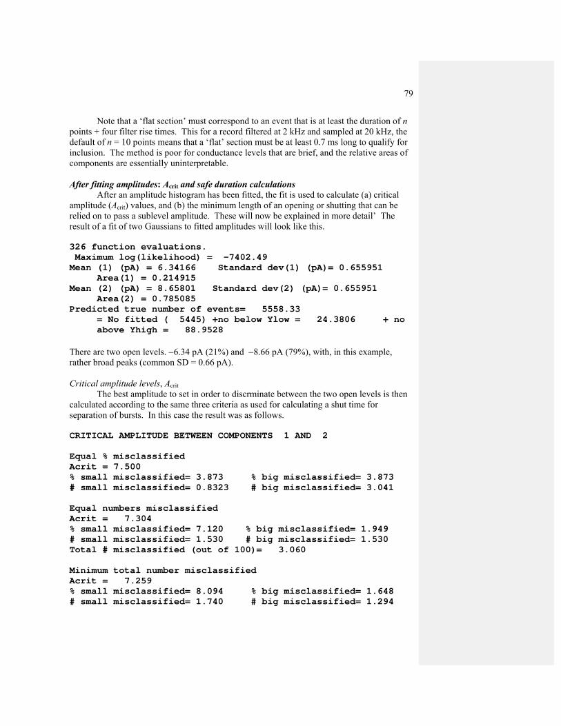
79

Note that a ‘flat section’ must correspond to an event that is at least the duration of n points + four filter rise times. This for a record filtered at 2 kHz and sampled at 20 kHz, the default of n = 10 points means that a ‘flat’ section must be at least 0.7 ms long to qualify for inclusion. The method is poor for conductance levels that are brief, and the relative areas of components are essentially uninterpretable. After fitting amplitudes: Acrit and safe duration calculations

After an amplitude histogram has been fitted, the fit is used to calculate (a) critical amplitude (Acrit) values, and (b) the minimum length of an opening or shutting that can be relied on to pass a sublevel amplitude. These will now be explained in more detail’ The result of a fit of two Gaussians to fitted amplitudes will look like this. 326 function evaluations. Maximum log(likelihood) = -7402.49 Mean (1) (pA) = 6.34166 Standard dev(1) (pA)= 0.655951

Area(1) = 0.214915 Mean (2) (pA) = 8.65801 Standard dev(2) (pA)= 0.655951

Area(2) = 0.785085 Predicted true number of events= 5558.33

= No fitted ( 5445) +no below Ylow = 24.3806 + no above Yhigh = 88.9528

There are two open levels. −6.34 pA (21%) and −8.66 pA (79%), with, in this example, rather broad peaks (common SD = 0.66 pA). Critical amplitude levels, Acrit The best amplitude to set in order to discrminate between the two open levels is then calculated according to the same three criteria as used for calculating a shut time for separation of bursts. In this case the result was as follows. CRITICAL AMPLITUDE BETWEEN COMPONENTS 1 AND 2 Equal % misclassified Acrit = 7.500 % small misclassified= 3.873 % big misclassified= 3.873 # small misclassified= 0.8323 # big misclassified= 3.041 Equal numbers misclassified Acrit = 7.304 % small misclassified= 7.120 % big misclassified= 1.949 # small misclassified= 1.530 # big misclassified= 1.530 Total # misclassified (out of 100)= 3.060 Minimum total number misclassified Acrit = 7.259 % small misclassified= 8.094 % big misclassified= 1.648 # small misclassified= 1.740 # big misclassified= 1.294

80

Total # misclassified (out of 100)= 3.034 Following this, the same sort of calculation as described by Howe et al. (1991) is performed. The idea is to calculate the duration of an event that is needed so that its amplitude reaches, or surpasses by one or two SD, a subconductance level. Minimum duration to reach sublevel CALCULATION OF EVENT DURATION NEEDED TO PASS SUBLEVEL Amplitude of MAIN level (pA) = 8.658 Calculate time for event to reach sublevel +/- n*sd: n = [2.0] = 1.0 Minimum usable open time (ms) calculated as duration of opening that reaches Acrit (pA)=sublevel + 1.0*SD Minimum usable shut time (ms) calculated as duration of shutting that reaches Acrit=full-(sublevel - 1.0*SD) If required level is < 0 or > 1, '-' is printed Sublevel SD ____ Open time____ ____ Shut time____ (pA ) (pA) Acrit Duration Acrit Duration 1 6.34 0.66 7.00 0.1153 2.97 0.0393 Thus open times shorter than 0.115 ms cannot be guaranteed to surpass the sublevel by one SD and we cannot therefore be sure whether shorter openings are to the sublevel or to the main level. Distributions for bursts of openings

Options for the definition of bursts There are three options, though normally only the first one is used. (1) Bursts to include ANY open state separated by shut periods that are all shorter than tcrit (normal definition). (2) Bursts consist of any series of openings to a specified amplitude (range), these openings being separated by periods in ANY other level (open or shut) that is (a) not in the specified amplitude range, and (b) has total duration < tcrit '. Burst ended by any sojourn longer than tcrit outside the specified range. This is the ''50pS/non-50pS'' print definition in which all amps NOT in range are treated as ''shut''. Looks at transitions from specified amp to all other states, and back. Bursts consist of any series of openings to a specified amplitude (range), these openings being separated by periods in ANY other level (open or shut) that is (a) not in the specified amplitude range, and (b) has total duration < tcrit ', (the ''50pS/non-50pS'' print definition in which all amps outside range are treated as ''shut'').

81

(3) Bursts consist of alternations between open (in specified amplitude range) and SHUT (<tcrit). Bursts consist of alternations open (in specified range) and SHUT (<tcrit). Burst ends when (a) shut period > tcrit found, OR (b) transition from specified open level to ANY other open level (whatever its duration) is found, OR (c) transition to shut period of ANY duration is found if the shut period is followed by transition to an opening outside the specified range. Looks at transitions from specified amplitude to brief shut states, and back.

Display of bursts

There is now an option to display the bursts in the raw digitised data (as long as this file is available of course). This uses a two window display (subroutine VSAMP) with the burst shown in the lower window, and a more compressed display in the upper window which shows the shut time on each side of the burst. The region coloured red in the upper window is what appears, expanded, in the lower window. The display in the lower window can be shifted left or right, and expanded or contracted. Cursors can be used (in the upper window) to define a new section for the expanded (lower) display. Data outside the region shown in the upper window cannot be shown at present. F1 key gives a brief description of each menu key. The first time you use the display you will be asked for the name of the continuous data file (CONSAM, or AXON data file; the name is remembered in the ekdist.ini file for the next run). The window below the display gives information about the burst on display (interval numbers in the burst, number of open periods per burst, total open time, shut

Distribution types for bursts (1) No of individual openings per burst (2) No of open periods per burst (=1+short gaps/bst) (3) Total burst length (4) Total burst length (exc time outside spec range) (5) Total open time per burst (6) Total open time per burst (exc time outside spec range) (7) Burst length for bursts with k apparent openings (or k or more) (8) Open time/burst for bursts with k apparent openings (or k or more) (9) Length of gaps within bursts (10) Length of open periods (1st, 2nd...) in a burst (11) Correlation of ith and jth opening in burst (12) Distribution of ''mean amplitudes'' of bursts (13) Distribution of ''mean amplitudes'' of bursts with signs reversed (14) Distribution of Popen for bursts (15) Print means for kth open period or shut time (16) Length of the last open period in burst' (17) Length of the last gap (shut time) in burst

82

time and total length, and Popen values (with and without the last open period included). When a valid value for the distribution is found it is displayed (as “dist = “) at the end of the first line (the value can be rejected by key 1 whenever the menu at the bottom has 1.REJECT showing). Distribution of Popen for bursts (option 14) When this option is used to find the Popen within a group of openings, it is common to omit the last opening in each burst (so there are equal numbers of open and shut times). It is also common to omit short bursts, e.g. those with less than 50 ms length, or with fewer than 10 openings (open periods) in the burst. Options for doing all these are presented. Bursts that are shorter than the specified length may, optionally, still displayed but are labelled (at end of the first text line) as REJECTED (TOO SHORT), and in this case the 1.REJECT button does not show –just hit 9.ACCEPT/NEXT. After display of the distribution of Popen values, it can be fitted.–The only option at present is to fit with Gaussian(s), which is not the theoretically-expected form, but may fit well enough to be useful. Number of openings or open periods per burst (geometric distributions) A new logarithmic display for geometric distributions as been included, which is not yet described in Colquhoun & Sigworth, 1995). Details will therefore be given now. This display is described in Wyllie et al., 2000, J. Phyiol. Single-channel analysis of a NMDA receptor possessing an amino acid point mutation in the region of the glutamate binding site).

Logarithmic display of geometric distributions Distributions such as that of the number of open periods per burst are expected to be described by mixtures of geometric distributions (Colquhoun & Hawkes, 1982). Observations are best fitted by maximum likelihood, as described by Colquhoun & Sigworth (1995). The conventional display of these distributions makes it hard to see, and compare, the tail of the distribution, which often has low amplitude. In the case of distributions of durations (e.g. shut times), this problem is usually solved by showing the results as distributions of log(duration), the square root of the number values normally being plotted, as here (ref***). This is not feasible in the case of a discrete variable such as the number of open periods per burst. This number, r say, can take only integer values, r = 1, 2, 3, . . . We have therefore introduced a display for geometric distributions which is analogous to that for log(duration). If the number of times a value equal ot r is observed is denoted f(r), then the display is constructed by plotting

)(rfr against log(r) (1) Recalling that the probability density function, g(x) say, of x = log(t) is given by

)()( tftxg = , (2) (Colquhoun & Sigworth, 1995), the new plot is seen to bear a close analogy to the distribution of log(duration), and becomes identical with the latter for geometric distributions with large means (it is close when the mean value of r is greater than 10 or so). In the case of

83

durations, the observations are grouped into bins whose boundaries are equally spaced on a logarithmic scale, and the frequency of observations in the lowest bins is low because the lowest bins are narrow. In the case of an integer variable the bin width cannot be altered, but the same effect is obtained by multiplying the observed frequency by r (compare eqs. 1 and 2) The simple geometric distribution with mean μ is

1111)(

−

⎟⎟⎠

⎞⎜⎜⎝

⎛−=

r

rPμμ

. (3)

Since r is a discrete variable, these probabilities exist only at r = 1, 2, 3, . . .. If we define G(r) = r P(r), then the ratio of two successive terms is

rrG

rG11

11

)1()(

−

−=

−μ , (4)

which is greater than one if and only if r < μ. Thus G(r) = r P(r) rises to a maximum at a value that is the integer part of μ (the mean rounded down to the nearest integer), and then declines. If μ happens to be an integer, which in general will not be so, then there will be two equal maxima, at r = μ −1 and at r = μ.. The envelope of the display, found by treating r as a continuous variable, has a maximum at r = −1/ln(1 − 1/μ), which approaches μ − 0.5 for large μ. Thus the peak of the display is close to the mean of the distribution, like the analogous distribution of log(duration), for which the peak is at the mean, τ. For geometric distributions with means smaller than 10 or so, the new plot has a different shape from the distribution of log(durations) and this is illustrated in Fig 1. Fig 1A shows the conventional display of the simple geometric distribution of P(r), with means μ = 1.1, 2, 5 and 10.Figure 1 B shows the same values, plotted in the new way, as )(rPr against log(r). The probabilities exist, of course, only at r = 1, 2, 3, . . ., and so should be plotted as points or vertical lines at these values of r. It may increase visibility if these points are joined, purely for cosmetic purposes, by straight lines., as in Fig 1.

Comment [DC3]: Page: 1 \pictures\wyllie\logGeo1.jpg and logGeo2.jpg from LogGeo.opj and LogGeo.xls

84

(8) Subconductance sequence listing

There are two main options AMPLITUDE SEQUENCE LISTING OPTIONS (1) List frequencies of direct transitions between amp levels. (2) List amplitude levels that occur in each burst

Both options require the definition of several amplitude ranges (‘windows’), which may or may not include the shut level. These will usually be defined on the basis of a fit to the amplitude distribution, the boundaries being based on the acrit values that discriminate best between the peaks on this distribution.

You also need to set the resolution to be used for open and shut times. The resolution for shut times will normally be that set at the start of the program (this is the default). But the resolution for open time must be bigger because we are interested in measured amplitudes so only openings that are long enough for their amplitude to be measured can be used (the default is two filter rise times, but this may be a bit short). You can set a different resolution for each amplitude window (and also for each file, if you are pooling more than one data file from SCAN). (1) List frequencies of direct transitions between amp levels.

The first option looks at direct transitions between one amplitude level and another, for all possible pairs, triplets etc of amplitude levels, wherever these sequences occur in the record. There is now an option to display the direct transitions. This uses a two window display (subroutine VSAMP) with the transition sequence (plus 10 ms on each side of it) in thelower window (the sequence itself is highlighted in purple). The upper window shows a more compressed display (50 ms on each side of the sequence) (see Burst distributions, above, for more details). (2) List amplitude levels that occur in each burst In this option the record is divided into bursts in the same was as when looking at distributions of burst length etc. This is designed to test which combinations of levels occur in bursts e.g. if there is a mixed population of channels is each activation characterised by a particular set of sublevels. The program lists something like the following (when three amplitude windows have been defined). Number of bursts that contain opening(s) to specified levels ONLY (NB : could also contain levels that are not in ANY specified amp range) Levels number percent 1 0 0.00 2 3 1.19 3 53 20.95

85

Distributions for single channels after a concentration jump SHUT TIMES AFTER JUMP

(1) Latency to the first opening (2) Length of nth shut time after t = 0 (3) Length of all shut times (and shut-shut correlation) (4) Mean length of nth shut time for n = 0, 1,.2, . . .

OPEN TIMES (1) Length of nth open period in the jump (2) Length of all open periods (3) Mean length of nth open period for n = 0, 1,.2, . . . (4) Number of open periods per jump (5) Mean open period adjacent to shut time in specified range (6) Mean open period adjacent to open period in specified range (7) Length of the last open period in the jump

TOTAL ACTIVATION OPTIONS (1) Time from t = 0 to end of last opening (2) Time from start of first opening to end of last (3) Total open time per jump (4) Popen within activation (exc latency) (5) Popen within activation (inc latency)

BURSTS WITHIN JUMPS (1) Total burst length (2) Total open time per burst (3) Number of open periods per burst (4) Number of bursts per jump

Combinations of 2 levels 1 2 1 0.40 1 3 93 36.76 2 3 2 0.79 Combinations of 3 levels 1 2 3 101 39.92 TOTALS 253 100.00 Note that the combination 1 2 means that these bursts have levels 1 and 2 ONLY, with no level 3. The results are listed with and without bursts that contain a single opening, and, if one of the levels is the shut level, they are also listed with and without the shut level. There is now an option to display the bursts. This uses a two window display (subroutine VSAMP) with the burst shown in the lower window, and a more compressed display in the upper window which shows the shut time on each side of the burst (see Burst distributions, above, for more details). The baseline (as defined in SCAN) is shown, together with dashed lines that show the boundaries of the amplitude windows (these lines can be hidden with key 8 if wished). If you choose to display bursts, a drop down menu appears that allows you to choose whether to display all bursts, or only those that contain specified amplitude levels. Options for distributions for single channels after a concentration jump

86

Correlations At various points throughout EKDIST you are offered the option to look for correlations between things like open-open times, shut-shut times and open-shut times. These options calculate (a) runs tests and (b) autocorrelation coefficients, by the methods described in Colquhoun & Sakmann (1985). Autocorrelation coefficients may be plotted against lag, at such plots are expected to decay to zero. in Colquhoun & Hawkes (1987). The question of the origin and meaning of such correlations is discussed in Single Channel Recording (Colquhoun & Hawkes, 1995, and references therein). The graphs are also plotted after transformation to Gaussian, though I’m not sure that this is much use. . A variable t, that follows a simple exponential distribution with mean t, can be transformed to a Gaussian variable, z, as follows

)/exp( τtq −= ))1(4log(5.0 qqx −−= π if q ≤ 0.5

))1(4log(5.0 qqx −−−= π if q > 0.5 765433 103728.410881.2108365.7 xxxxz −−− ×+×−×+=

This transformation results in a Gaussian variate only in the case of a simple exponential, but the program uses it whatever the distribution of the intervals. The calculation of quantities such as the correlation between an open time an the next (next but one etc), and similar calculations for shut-shut and open-shut, has been found to be quite sensitive to instabilities in the data. The usual effect of instability (baseline drift or step changes) seems to be to give a positive correlation that does not decay with lag. A warning to inspect stability plots carefully before calculating correlations has added to EKDIST. If the correlation coefficient is found not to decay to zero, the reason is probably either

(1) You have not calculated large enough lags, or (2) The data are not stable

More sophisticated approaches to looking at correlations are available under main menu option (9) Bivariate distributions and dependency plots Fitting of distributions ===details to be finished Simultaneous fits and randomisation tests Usually only one data set is fitted at a time (though it may consist of several comparable experiments pooled together). If more than one data is specified then it is possible to do the following tricks.

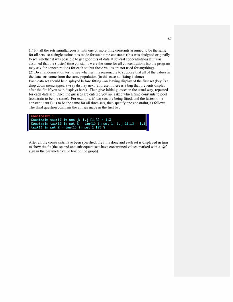
87

(1) Fit all the sets simultaneously with one or more time constants assumed to be the same for all sets, so a single estimate is made for such time constants (this was designed originally to see whether it was possible to get good fits of data at several concentrations if it was assumed that the (faster) time constants were the same for all concentrations (so the program may ask for concentrations for each set but these values are not used for anything). (2) Do a randomisation test to see whether it is reasonable to suppose that all of the values in the data sets come from the same population (in this case no fitting is done) Each data set should be displayed before fitting –on leaving display of the first set (key 9) a drop down menu appears –say display next (at present there is a bug that prevents display after the fits if you skip displays here). Then give initial guesses in the usual way, repeated for each data set. Once the guesses are entered you are asked which time constants to pool (constrain to be the same). For example, if two sets are being fitted, and the fastest time constant, tau(1), is to be the same for all three sets, then specify one constraint, as follows. The third question confirms the entries made in the first two.

After all the constraints have been specified, the fit is done and each set is displayed in turn to show the fit (the second and subsequent sets have constrained values marked with a ‘@’ sign in the parameter value box on the graph).

89

Help notes for HJCFIT Maximum likelihood fitting of a mechanism with exact allowance for missed brief events

This program uses the exact solutions for single channel distributions with missed events

derived by Hawkes et al.,(1990, 1992). The maximum likelihood method that was described by

Colquhoun et al. (1996), and this method is implemented in HJCFIT. The equations that are used

will (almost) all be found in Colquhoun Hawkes & Srodzinski (1996). A brief description of the

relevant theory is given in HJCNOTES.DOC, and these notes are appended to the end of this

manual.

These notes refer to the latest version which takes up to 100 states and 10 ligands. For detailed

notes on the theory click here.

Some general points concerning the running of the program

The program is similar to other DC programmes in general approach. In particular the

graphics subroutines are the same as in other programs, so they are described in a separate plot

section.

When you run any of the programs, a blue window appears at the beginning asking if

you want to keep the print-out in a disk file, HJCFIT.PRT. Press 1, 2, 3 or 4 (e.g. on numeric

keypad). No print out is kept if the items one and two are set to ‘N’. If the first item only is ‘Y’

then a new print file is started, which overwrites any existing file (without warning!). If both are

set to ‘Y’ then the printout is appended to the existing print out. The safest procedure is to set

both to ‘Y’ and then press F2 to keep this setting as the default for next time

The first time you run the program, choose option 3, set up this computer. Give the

computer a name (this, together with date and time, appears on all the print files). Give the

number of disk partitions (safest to say 26 for networked machines). State which disk partition

the print-out files are to be written to. State the printer port is to be used; at present this must be

LPT1 if you want graphical output (network printer is O.K. as long as it is called LPT1). Under

Windows 2000 (at least) it is also possible to print on a USB printer (ask DC for details), but still

90

specify LPT1 here. And say whether you have a colour screen. This information is kept in a

file called C:\DCPROGS.INI which is referred to every time you run a program (it is created the

first time you do this, and is always in C:\ wherever you put the programs themselves)

Some general notes about keyboard input Numerical input. All input is read in ASCII form so that it is not essential, for example,

to have a decimal point in floating point numbers (as it is in basic Fortran). Thus 200, 200.,

200.00, 2e2, 2.e2 are all acceptable inputs for the floating point number 200.

If asked for two (occasionally 3) numbers at once, as for example ‘Xmin, Xmax = ‘, then

enter two numbers separated by a comma.

Most (but not all) inputs have a default (in square brackets) and hitting enter with typing

anything gives this default value. When 2 numbers are input, and the default is OK for one but

not the other, then only the one to be changed need be entered, e.g. in response to ‘Xmin, Xmax

[0,10] = ‘, typing only ‘1’ gives Xmin=1., Xmax=10., and typing only ‘,20’ (with comma before

20) would give Xmin = 0., Xmax = 20.

Usually the numlock key switches itself on so you can use numerical keypad.

Yes/No input. Type ‘Y’ or ‘N’ in response (upper or lower case). Again there is usually

a default, as, in ‘Try again [Y] ?’. Hitting enter gives the default and hitting INS key gives

the opposite of the default (so it is rarely necessary to use the ‘y’ or ‘n’ keys). Usually the

numlock key switches itself on so you can use numerical keypad.

Summary of stages in an HJCFIT analysis These notes refer to the latest version (Aug-03), that takes up to 100 states and 10 ligands.

Quite a lot of things have to be specified to run the program. In summary, these are as

follows.

(1) Define which mechanism is to be fitted. If the default mechanism from the last run is not

right, then choose a different one from the list, or define a new one. (At this stage the set of

91

values for the rate constants that was stored with the model in QMECHS.MEC is also read in, but

these are not used or displayed now, that is done later in step 10). If you are doing a simulation,

the mechanism used for simulation is specified first, then the mechanism to be fitted (which may

be different). Note the file that contains records of mechanisms and rates was formerly

called, by default, qmechs.dat. This file contains many records each of which defines a

mechanism and a set or rate constants for that mechanism. The default extension has now

been changed from .dat to .mec to make the files more easily recognisable but the name

does not matter –you can type in any name (remember it must have 8.3 format).

If the mechanism contains cycles then you are asked here to choose between two methods for

dealing with them (see ***)

===up to here!

(2) Specify the data to be fitted. These are the output from SCAN (one or more SCAN.SCN files, or

files from the old style SCANDAT.DAT discs). There is now an option (2) to use an internally-

generated simulated .SCN file (simulated .SCN files generated by SCSIM.EXE should be analysed as

though they were experimental files)

(3) Specify the resolution to be imposed (see EKDIST notes. ekhelp.doc, for details).

(4) Inspect stability plots, and, if really necessary, excise some parts of the record

(5) Specify whether or not the entire experimental record is to be analysed as though it came

from one individual channel. If not, decide how the record is to divided into groups of openings

all of which do come from one channel only (see below, and HJCNOTES.DOC).

(6) Decide whether to set long open times as unusable (this is usually done only if a mistake in

scan has caused spuriously long openings to appear to be present).

(7) Specify the ligand concentration(s) for each data set.

(8) Specify which rate constants (if any) are to be constrained to be a fixed multiple of another

(see below, and HJCNOTES).

92

(9) Specify which rate constants (if any) are to be constrained by being given a value that

produces a specified EC50.

(10) Specify the rate constants to be used for initial guesses. If you asked for simulated data to

be generated with HJCFIT, you are also asked (first) for the ‘true’ rate constant values to be used

for the simulation.

(11) Specify which rate constants (if any) are to have their values fixed, (see below, and

HJCNOTES). Also specify the maximum allowable value for any association rate constant.

(12) Specify the inputs for the simplex optimisation (the defaults are usually fine), and wait for

the fit to converge (anything from 2 minutes to 4 hours).

(13) Check the quality of the fit by seeing how well the fitted rate constants describe the data

(both unconditional and conditional distributions).

(14) Save the fitted values of rate constants

(15) Calculate standard deviations of, and correlations between, the fitted rate constants (see

below, and HJCNOTES.DOC).

Each of these stages will now be described in more detail.

First specify an initialisation file (default name, HJCFIT.INI). For some problems the number of

inputs that are needed is large, and it is usual to save all the details in HJCFIT.INI. That allows the

same problem to be run again using the same inputs as last time, simply by hitting <enter> to

accept all the defaults. It is usually convenient to save the ini file under a distinctive name

(remember DOS file names must be 8+3 characters). This name can be typed in, e.g.

Name for hjcfit.ini file: (use home/end/arrows/bs/ins/del)

HJCdemo.INI.............................

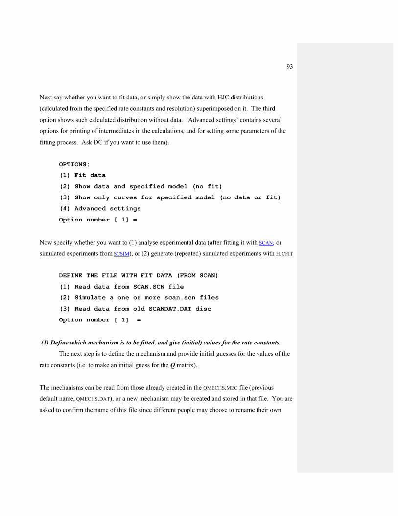
93

Next say whether you want to fit data, or simply show the data with HJC distributions

(calculated from the specified rate constants and resolution) superimposed on it. The third

option shows such calculated distribution without data. ‘Advanced settings’ contains several

options for printing of intermediates in the calculations, and for setting some parameters of the

fitting process. Ask DC if you want to use them).

OPTIONS:

(1) Fit data

(2) Show data and specified model (no fit)

(3) Show only curves for specified model (no data or fit)

(4) Advanced settings

Option number [ 1] =

Now specify whether you want to (1) analyse experimental data (after fitting it with SCAN, or

simulated experiments from SCSIM), or (2) generate (repeated) simulated experiments with HJCFIT

DEFINE THE FILE WITH FIT DATA (FROM SCAN)

(1) Read data from SCAN.SCN file

(2) Simulate a one or more scan.scn files

(3) Read data from old SCANDAT.DAT disc

Option number [ 1] =

(1) Define which mechanism is to be fitted, and give (initial) values for the rate constants.

The next step is to define the mechanism and provide initial guesses for the values of the

rate constants (i.e. to make an initial guess for the Q matrix).

The mechanisms can be read from those already created in the QMECHS.MEC file (previous

default name, QMECHS.DAT), or a new mechanism may be created and stored in that file. You are

asked to confirm the name of this file since different people may choose to rename their own

94

(mine has been renamed as qmechsDC.dat, and the equivalent name for the demonstration files

on the web is qmechdem.mec).

-----------------------------------------------------------

-

Name/path for models file: (use home/end/arrows/bs/ins/del)

qmechdem.mec............................

Now there are several options DEFINE THE REACTION MECHANISM Last run used mechanism # 29: Two unequal bindings (Milone et al 1997) with rates from file # 51: (1) Use mechanism as in last run (2) Choose a mechanism from those already defined (3) Define a completely new mechanism (4) Define a new mechanism by modifying an existing one (5) List all the models in QMECHS.MEC (new version) (6) Exit Option number [ 1] =

Enter 1, 2, 3, . . , or 6

Option 1 reads, from HJCFIT.INI, both the mechanism and the rate constants that were used in the

last run (either or both can be changed however).

Option 2 allows choice of any of the mechanisms that have already been defined (they are stored

in the file QMECHS.MEC). If the name of the QMECHS file is not the same is in the last run, then

you will be forced to use option 2 (because the same mechanism may have a different number in

different QMECHS file).

Options 3 and 4 allow definition of new mechanism, which can then be stored in QMECHS.MEC fo

r subsequent use.

95

Definition of a new mechanism

Choosing option 3 displays a blank blue chessboard (option 4 displays a predefined

mechanism). Put the states in the blue squares and the connections between them in the black

squares). The F1 key displays help for definition of the mechanism. States are denoted by a

letter which must be ‘c’ or ‘o’ (closed and open, respectively), and by a state number (1 to 99, or

0 to denote 10). For state numbers greater than 10, the initial letter is omitted. The open states

must have the lowest numbers (1, 2, . . .), according to our usual convention (Colquhoun &

Hawkes, 1982). If it is intended to calculate burst properties (e.g. in SCBST.EXE) then short-lived

shut states should have the next lowest numbers (though states can always be renumbered at a

later stage). For example states in the del Castillo-Katz would be numbered c3, c2, o1.

Connections between states are states are entered with ‘ − ‘(minus) for horizontals, ‘!’ for

verticals, and home, end Pgup. PgDn for corners (corners can be used only to join horizontal or

vertical connectors -they cannot join states directly). For example, the mechanism discussed in

HJCNOTES.DOC would be entered thus:

c5 | c4 − o1 | | c3 − o2 Once the mechanism has been drawn correctly hit the Esc key to finish. The reaction mechanism

diagram employs line-drawing characters that are above ascii 127, and which are not present in

all character sets. In our experience they generally print correctly with the default character set

on inkjet printers, but for laser printers you may have to change the default character set to get

correct printing.

This entry method cannot have links between states that cross, and cannot define 3D

mechanisms. Such complex mechanisms can be defined by manual entry of the rate constants

and connections, or with the new Windows version that is under development now.

The number of open states (denoted kA),and the number of shut states (denoted kF) is

printed. You are then asked to define the number of short-lived (‘within-burst’) shut states (kB),

96

the number of long-lived (‘between burst’) shut states (kC), and the number of long-lived

(‘between cluster’) shut states (kD). The states in set A (open) must have higher state numbers

than those in set B, and so on. These values are relevant to the definition of bursts, and clusters

of burst, according to Colquhoun & Hawkes (1982; see 1995 also), but they are not relevant to

HJCFIT, so it does not matter what values are given here (as long as kB + kC + kD = kF ). The

connections between states, and any cycles in the mechanism are now printed out, and it should

be checked that the program has got them right.

If there are cycles, you are asked

Should ALL cycles be constrained my microscopic reversibility?

In the latest version it is possible. if you say ‘N’ here, to specify that some cycles do and others

do not. If you specified that microscopic reversibility is to be obeyed, then say which rate

constant in each cycle is to be calculated from all the others (e.g. enter ‘2,1’ for the scheme

above to calculate the dissociation rate constant for loss of an agonist molecule from the doubly-

occupied open state).

Next specify how many ligands are present (at the moment this must be 0, 1 or 2), and

then the number of rate constants that should be multiplied by concentration (i.e. the number of

association rate constants in the mechanism, with dimensions M−1s−1). For each such rate

constant you must then specify which connection it is (from the ith state to jth state) by entering

values for i, j (e.g. enter ‘3,2’ for the del Castillo-Katz mechanism, ‘5,4’ , ‘4.3’ and ‘1,2’ in the

example above), and if more than one ligand is present, specify which of the ligands is being

bound for each of these association reactions.

If the mechanism is new, there will be no stored rate constants for it, so there is no point

in trying to read them. A blue window appears (with the mechanism you just defined shown to

the left of the window, for reference). The association rate constants (and those calculated by

microscopic reversibility, if any) are already marked (at the leftmost edge of the window). The

F1 key brings up a help window that explains the notation, and how to enter values. A name for

each rate constant is entered into the column headed Rate constant (any ASCII text can be used),

and the numerical value for that rate constant (i.e. the initial guess for a fit) is entered into the

rightmost column (headed Value). The name given to a parameter that includes a ‘statistical

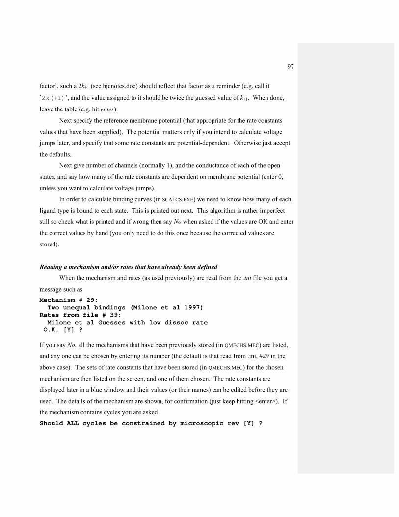
97

factor’, such a 2k+1 (see hjcnotes.doc) should reflect that factor as a reminder (e.g. call it

’2k(+1)’, and the value assigned to it should be twice the guessed value of k+1. When done,

leave the table (e.g. hit enter).

Next specify the reference membrane potential (that appropriate for the rate constants

values that have been supplied). The potential matters only if you intend to calculate voltage

jumps later, and specify that some rate constants are potential-dependent. Otherwise just accept

the defaults.

Next give number of channels (normally 1), and the conductance of each of the open

states, and say how many of the rate constants are dependent on membrane potential (enter 0,

unless you want to calculate voltage jumps).

In order to calculate binding curves (in SCALCS.EXE) we need to know how many of each

ligand type is bound to each state. This is printed out next. This algorithm is rather imperfect

still so check what is printed and if wrong then say No when asked if the values are OK and enter

the correct values by hand (you only need to do this once because the corrected values are

stored).

Reading a mechanism and/or rates that have already been defined

When the mechanism and rates (as used previously) are read from the .ini file you get a

message such as Mechanism # 29: Two unequal bindings (Milone et al 1997) Rates from file # 39: Milone et al Guesses with low dissoc rate O.K. [Y] ? If you say No, all the mechanisms that have been previously stored (in QMECHS.MEC) are listed,

and any one can be chosen by entering its number (the default is that read from .ini, #29 in the

above case). The sets of rate constants that have been stored (in QMECHS.MEC) for the chosen

mechanism are then listed on the screen, and one of them chosen. The rate constants are

displayed later in a blue window and their values (or their names) can be edited before they are

used. The details of the mechanism are shown, for confirmation (just keep hitting <enter>). If

the mechanism contains cycles you are asked Should ALL cycles be constrained by microscopic rev [Y] ?

98

If you say ‘N’ then you can set individual cycles (if there is more than one) to be constrained to

obey macroscopic reversibility, or not to be so constrained.

After the mechanism has been defined, there is an option to keep either or both for future

use by writing the to a QMECHS.MEC file (this dies not have to be the same one that was read

form).

Simulated experiments generated in HJCFIT

If you are doing simulations –then the first mechanism to be requested is that used to generate

the simulated data (the windows appear in green). You are asked whether the same mechanism

should be used for fitting. It is possible to specify a different mechanism for fitting, in which

case the whole of the previous section is repeated (but the windows are now the usual blue

colour) to define it. For example you might simulate data using a mechanism that includes

desensitised state(s), but fit it (in bursts) without the desensitised state.

(2) Specify the data to be fitted

The experimental data consists of one or more steady state single channel recordings that

have been fitted with SCAN, so the SCAN.SCN (also known as SCAN.DAT) files that contain the

results of this fitting must be specified. Several (up to 10) data sets can be specified, and the

agonist concentration, resolution etc may be different for each set. Each set can consist of more

than one SCAN.SCN files that are pooled into a single data set (all of these files must have the

same concentration, resolution etc). This input consists of a sequence of open times, their

amplitudes and shut times (in the order that they occur). At present the program requires that

these have been fitted by SCAN, because additional information about unusable openings,

indefinable amplitudes etc. is expected that other programs do not provide.

The names of the files, together with resolutions, concentrations, constraints etc. are kept

in HJCFIT.INI, and are presented as defaults so it is easy to run HJCFIT several times with the same

data.

The name of the data file(s) used in the last run are displayed, and can be accepted

straight away. If you want to analyse a different experiment, not the same one again, then you

are asked how many data sets (e.g. different concentrations) you wish to fit simultaneously, and

99

for each set, how many SCAN.SCN files are to be pooled (latter is normally 1).

Simulated experiments generated in HJCFIT

In the case of internally-generated simulated data there is no SCN data file, and you are

asked only for the number of channel transitions to be generated, ligand concentration(s),

resolution, the seeds for the random number generator (NB if the default seeds contain zeros

your RANDOM.DAT file is invalid: enter 3 random integers separated by commas), and the names

for the files where the output is to be written. The is another program (SIMAN.EXE) for analysing

this output (not yet on web site)

Next you can specify (or confirm) the name of the file where queued plots are to go (e.g.

191016h1.plq).

(3) Specify the resolution

This section is exactly as in EKDIST (see EKDIST notes for a detailed description), except

that the HJC theory requires that a single resolution be imposed, the same for both open and shut

times. The number of resolved intervals is then printed.

(4) Show stability plots?

There is next an option to show stability plots for amplitudes and/or for open and shut

times (exactly as in EKDIST). After the display is left you have, as in EKDIST, a chance to define

areas to be omitted from the analysis, by means of cursors on the plot. The omitted regions are

recorded in the .INI file so the analysis can be repeated with identical omissions.

(4a) New option (June 2002) [This is now found under ‘advanced settings’ at the start]

A new option, that will rarely be needed, allows open periods to be excluded form the analysis if

the are bordered in BOTH sides by shut time in a specified range (as used by Hatton et al.,

2002). After the stability plots you are asked Exclude any open times on basis of adjacent shut times [N] ?

Normally the default (No) is appropriate. If you say Yes, you are asked (separately for each set)

to confirm this decision, and if the option is used you specify the shut time range Lower, upper limits for length of adjacent gap (ms) =

100

When this is used, the open periods to be eliminated are concatenated with the bordering shut

times into one long shut time, before fitting (and they are similarly eliminated for the data

histogram displayed after fitting. The number of open periods that are so excluded is printed, for

each set, just before ‘Final values of rate constants’.

(5) Does whole the record contain only one channel? If not, divide the record into groups

each of do arise from one channel by defining a critical shut time

Next specify whether or not the whole single channel record arose from only one

individual channel.

Did patch contain only one channel (AND all relevant states

are included in the mechanism being fitted) [N] ?

Ideally the answer would always be Yes, so the whole record could be analysed as one long

sequence. However in most cases this will probably not be the true, and when it is not we must

now decide what to do.

When more than one channel is present it would be possible, in principle, to do an optimum

analysis if the number of channels in the patch were known. However HJCFIT cannot do this (the

necessary theory has yet to be worked out), and in any case it is rare that the number of channels

in the patch can be estimated with any certainty. The solution to this problem is to define

sections of the record that we can be sure arise from a single channel. This is done by defining a

critical shut time to divide the record into groups of openings. Therefore if the answer to the last

question was No then you must now specify the critical shut time, tcrit, for division of the record

into one-channel groups (this would normally be found from the shut time distribution -values of

tcrit are printed in EKDIST after fitting the shut time distribution).

Set 1: critical shut time (tcrit) (ms) [3.5] =

There are two common situations where division into groups is possible.

(a) In recordings made at high agonist concentrations, long groups of openings occur within

which the channel is open for a substantial fraction of the time, so that the presence of

101

more than one channel would be obvious. These clusters of openings are separated by

more or less long shut times, during which all the channels in the patch are desensitised

((Sakmann et al., 1980)). These groups of openings can be demarcated by defining a

critical shut time, tcrit, such that any shut time longer than tcrit is deemed to end a group.

(b) In records made at low agonist concentrations, in which the channel is open for only a small

fraction of the time it is usually impossible to know how many channels are present.

However individual activations of the channel usually consist of groups of openings

(‘bursts’) separated by more-or-less short shut times. Usually it is clear that the openings

in one activation all arise from the same individual channel, and this was first exploited

by (Colquhoun & Sakmann, 1985;Colquhoun & Sakmann, 1981) to allow information

about mechanisms to be extracted from the recording. At low enough agonist

concentrations these activations will be separated by long shut times, so again these

groups of openings can be demarcated by defining a critical shut time, tcrit, such that any

shut time longer than tcrit is deemed to end a group.

Once a critical shut time has been defined, the likelihood is then calculated separately for each

group, and the overall likelihood that is maximised is found as the product of these separate

group likelihoods (see HJCNOTES.DOC). Notice that, almost always, some shut times will have

already been labelled as unusable during the analysis of the raw data in SCAN. This is done if, for

example, an occasional double opening has to be excluded from the analysis, or if the patch

temporarily becomes noisy. It is important that such events should be labelled because HJCFIT

requires that events are in the actual order in which they occur. The calculation of the likelihood

of the entire sequence of open and shut times must stop when an unusable shut time is

encountered, and be restarted at the next good opening. The effect of the presence of unusable

shut times is to break the record up into groups of openings for each of which the likelihood is

calculated separately, the overall likelihood that is maximised being the product of the separate

likelihoods for each group (see HJCNOTES.DOC, eq. 7.3).

If you said that the whole record was not from one channel then the strategy to be

adopted depends on whether the long shut times that separate one-channel groups are spent in

states that are included in the mechanism to be fitted.

102

Set 1: Are long shut times spent in states that are included in the mechanism being fitted [Y means that CHS vectors are used for the start and end of bursts] [Y] ?

For example, for a very low concentration record the answer should be Yes (Y). But for high

concentration records the answer would be Yes only if the mechanism being fitted includes

desensitised state(s) explicitly. If it does not (as in the example in HJCNOTES.DOC), the answer

should be no (N).

The answer to this last question controls the way in which the program calculates the

initial and final vectors for each group of openings (see HJCNOTES.DOC). If the answer is yes,

then correct allowance can be made for the nature of the states in which the long shut times are

spent. Because we do not know the number of channels in the patch, we do not know the true

length of the long shut times (which is why they cannot be included in the likelihood

calculation), but we do know that they are longer than tcrit, and this information can be used, for

example, to calculate correctly the probability that the first opening of the next group of opening

starts in each of the open states. If the answer to this question is No, then the normal steady-

state initial vector has to be used, though this will not be quite right if the next opening follows

emergence of a channel from desensitised state(s). The most common reason for answering No

is because desensitised states are not included in the mechanism, but in such experiments the

groups of openings are quite long which means that a small error in the initial vector causes little

error in the final result.

If the record is divided into bursts then long shut times are already excluded so the next question

does not appear. If, on the other hand, the record is analysed as though it all came from a one-

channel patch then you are asked the following question Data set 1 Long shut times can be set as bad (e.g. because they result from fitting errors, or from states that are visited very rarely, or from states that are not included in the mechanism being fitted). Set very long shut times as bad [N] ?

If you say yes you are asked

103

Set 1: set all shut times as bad if longer than t (ms) [100] =

The effect of this is to set the selected shut times unusable in the same way that some ar set as

unusable in SCAN.

(6) Decide whether to set long open times as unusable

This will usually be necessary only when a mistake has been made in SCAN, such that one

or two erroneously long openings appear in the results. It might also be used if there are a few

genuine extra long openings that are too few in number to be fitted.

Set 1: set all open times as bad if longer than t (ms) [20] =

The effect of setting them unusable is that the group of openings for which likelihood is

calculated (see HJCNOTES.DOC) is ended at the previous good shut time, and a new group is

started at the next good opening.

(7) Specify the ligand concentration(s) for each data set

Next state the ligand concentrations that were used for each data set. (One aim of fitting

simultaneously two (or more) data sets, obtained at different concentrations, is to see whether the

mechanism can predict correctly the observed concentration-dependence.)

(8) Specify which rate constants (if any) are to be constrained to be a fixed multiple of

another, or to have their values fixed,

Despite the fact that openings and shuttings, and their sequence, contribute information

for the fitting, it is possible (probably usual) that a single record will not be sufficient to define

all the parameters (rate constants). It is therefore often necessary to reduce the number of free

parameters (the ones that HJCFIT attempts to find values for). You are asked how many

parameters should be constrained, and how many should be fixed.

For example, for a mechanism with two bindings (e.g. as in HJCNOTES.DOC), a run

at low concentration will almost certainly have insufficient information to tell whether or not the

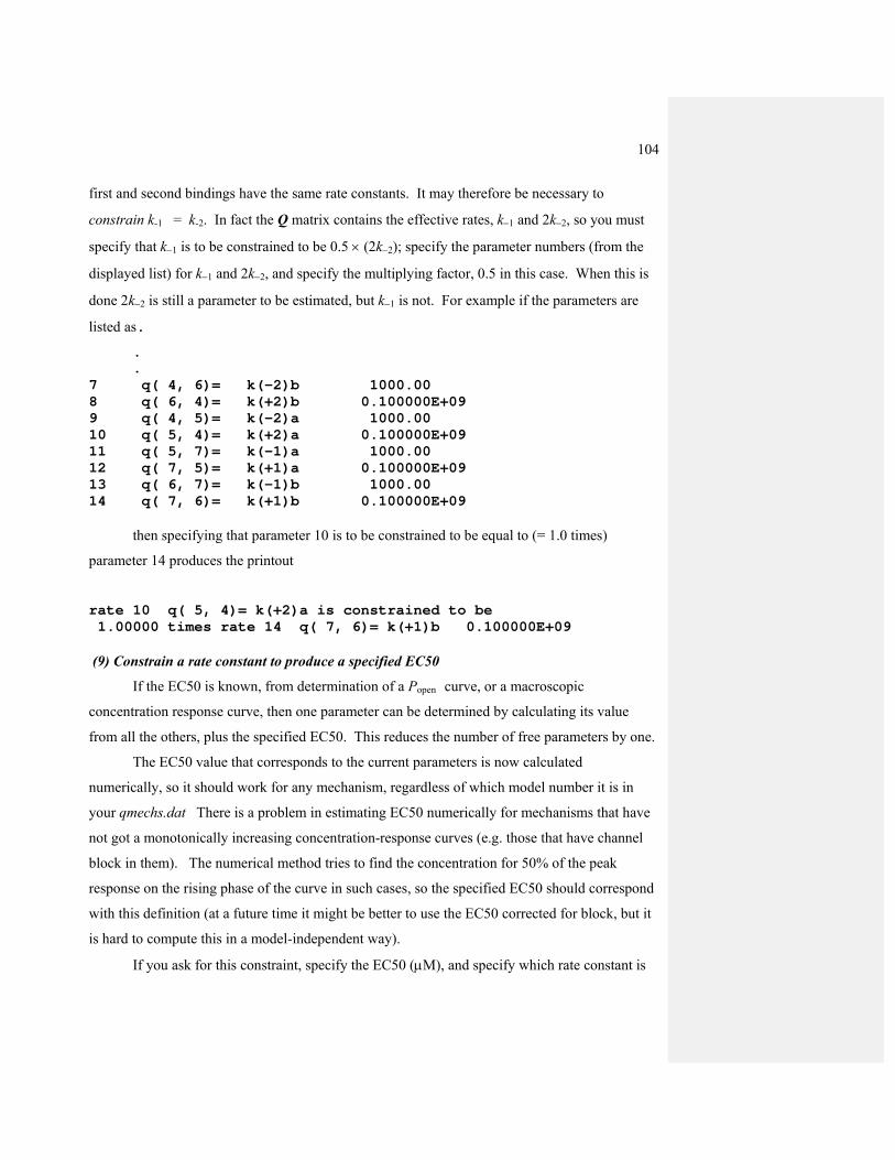
104

first and second bindings have the same rate constants. It may therefore be necessary to

constrain k-1 = k-2. In fact the Q matrix contains the effective rates, k−1 and 2k−2, so you must

specify that k−1 is to be constrained to be 0.5 × (2k−2); specify the parameter numbers (from the

displayed list) for k−1 and 2k−2, and specify the multiplying factor, 0.5 in this case. When this is

done 2k−2 is still a parameter to be estimated, but k−1 is not. For example if the parameters are

listed as.

.

. 7 q( 4, 6)= k(-2)b 1000.00 8 q( 6, 4)= k(+2)b 0.100000E+09 9 q( 4, 5)= k(-2)a 1000.00 10 q( 5, 4)= k(+2)a 0.100000E+09 11 q( 5, 7)= k(-1)a 1000.00 12 q( 7, 5)= k(+1)a 0.100000E+09 13 q( 6, 7)= k(-1)b 1000.00 14 q( 7, 6)= k(+1)b 0.100000E+09

then specifying that parameter 10 is to be constrained to be equal to (= 1.0 times)

parameter 14 produces the printout

rate 10 q( 5, 4)= k(+2)a is constrained to be 1.00000 times rate 14 q( 7, 6)= k(+1)b 0.100000E+09

(9) Constrain a rate constant to produce a specified EC50

If the EC50 is known, from determination of a Popen curve, or a macroscopic

concentration response curve, then one parameter can be determined by calculating its value

from all the others, plus the specified EC50. This reduces the number of free parameters by one.

The EC50 value that corresponds to the current parameters is now calculated

numerically, so it should work for any mechanism, regardless of which model number it is in

your qmechs.dat There is a problem in estimating EC50 numerically for mechanisms that have

not got a monotonically increasing concentration-response curves (e.g. those that have channel

block in them). The numerical method tries to find the concentration for 50% of the peak

response on the rising phase of the curve in such cases, so the specified EC50 should correspond

with this definition (at a future time it might be better to use the EC50 corrected for block, but it

is hard to compute this in a model-independent way).

If you ask for this constraint, specify the EC50 (μM), and specify which rate constant is

105

to be calculated from it. (e.g. specify 7,6 to constrain q(7,6), see below, and HJCNOTES).

You must also specify next, a range of values within which the constrained rate constant

must lie. For example when, as in the example, it is an association rate constant, it might be

restricted to the range 106 to 1012 M−1s−1. The purpose of this is to (a) prevent the production of

estimates that make no physical sense, and (b) to prevent the program crashing if the value of a

rate constant becomes absurdly large.

If the program cannot find any value for the rate constant (within the specified range) that

produces the specified EC50, then a penalty function method is used to steer the fit away from

the current parameter values. The penalty consists, by default, of subtracting 1 log-likelihood

unit from the likelihood for every 10% error in the best attainable EC50 estimate. You can now

specify how big the penalty is, because after giving the upper and lower limits for the

constrained rate, you are asked Factor for penalty function[10] =

If this factor (default value =10) is denoted f, the required ec50 is e50 and the EC50 calculated

from the current set of parameters is E50, the penalty to be subtracted from the log(likelihood) is

if E50, > e50,

or

50

5050 )(E

Eeabsfp

−= if E50, < e50,

(if E50 < 10-8. p =100 is used to prevent zero divide).

Setting a large enough penalty factor should usually be able to enforce the required EC50,

though possibly at the cost of a poor fit to the distributions.

If the penalty is still in effect when convergence is attained then a message to that effect is

printed, but in all cases tried so far, the penalty has been needed only during the early stages of

the fit and eventually values have been found that produce the required EC50, so the final

(maximum) likelihood has no penalty included in it.

For example, if this is done, the print file will include a statement such as Rate 14 q( 7, 6) = k(+1)b is constrained to give

50

5050 )(e

Eeabsfp −=

106

EC50 = 10.0000 micromolar

(10) Define values for the rate constants

It is always necessary to specify values of rate constants as the initial guesses for the fit (if the fit

is skipped, then the distributions that correspond with these rate constants are plotted). A list is

shown of all the sets of rate constants that have been defined (in your QMECHS.DAT file) for the

mechanism that was specified at the beginning. These values are displayed in a blue window,

with all of the specified constraints applied to them (in earlier versions, the rates were specified

before the constraints so this could not be done). If you change any of the values in the blue

window, the change will be printed to the disc file, and the window will be displayed again, with

the constraints re-calculated. If a rate constant(s) are to be fixed, it is simplest to put the value at

which you wish it to be fixed in the blue window (see next step). If the rate constants are

changed you may wish to save the values as a new record in QMECHS.DAT.

If you asked for simulated data to be used, you are asked first for which set of pre-defined rate

constants are to be used as the ‘true’ values that are used to generate the data. These appear in a

green window, and can be altered at this stage, as for the initial guesses. If you chose to simulate

the data using a mechanism different from that used for fitting then a warning is displayed to

remind you that it is your responsibility to ensure that the rate constants specified for simulation

obey all the constraints that you wish. The constraints are applied to the simulation rate constants

for you only in the case where the same mechanism is used for both simulation and fit (simply to

avoid having to type in a separate set of constraints for the former).

(11) Fix the values of rate constant(s), and set maximum for association rate constants

It will always help the fitting if some parameters can be fixed, e.g. at values determined

previously from runs at different concentrations, or different experiments.

If all openings are not from the same channel, so the openings are fitted in groups

(defined by tcrit), then information from long shut periods is lost. For example this may mean it

is not known how frequent activations are (for one channel), and this means that the forward

binding rates cannot be determined from the data. In this case it will probably be necessary to fix

107

say k+1 to some plausible value, e.g. 108 (M−1 s−1), (and also constrain k+2 to be half the fixed

value of 2k+1 , or just fix k+2 too). For example, if one parameter, say #14, is specified as fixed

the printout states

The following parameters are fixed: 14 q( 7, 6)= k(+1)b 0.100000E+09

After this you are asked what should be the maximum allowable value for any association

rate constant. The first time this is used the default value is 109 M−1s−1. If you want no

constraint then just specify a very large value here. In general values much bigger than 109

M−1s−1. are physically implausible (except for protons), so this constraint may be useful to obtain

the best fit that is possible with a physically realistic value for association rate constants. Note

that only association rate constants that are fitted freely can be constrained in this way (not those

that are found as a multiple of another parameter, or calculated by microscopic reversibility)

(12) The fitting process

In HJCFIT you are now asked if you want to skip the fitting process and simply plot curves

based on the supplied parameters. If you do not skip the fitting it is now done, using the Simplex

algorithm to maximise the likelihood, which is calculated as described in the theory notes.

Fitting using log(rate constant)

Recently (January 2002) the option was added was to use, with the simplex algorithm, the log of

the rat constant rather than the rate constant itself. This will influence the way in which the path

taken while searching for the maximum, but should not change the final results (maximum

likelihood estimates are invariant under transformations). This strategy seems to be so

successful that it has now been made the default option. If you want to use the original method say

No when asked "Use log(rate constant) in Simplex ?" Some notes on this

approach follow.

The main reason for trying this method was so that the initial step size in the simplex search The log rates

are used only within simplex, so they affect the direction of the search but should not affect the final value

obtained. When using this method was not equal in each direction. For example of the initial guess is

108

1000 (/s) it is hard to explore a large range of possible values because you cant take a step in each

direction of more than 1000 without getting a negative rate -therefore the initial step cannot go above

2000.

An additional advantage of the log(rate) method is that there is no need to use the constraint that rates

must be positive -however negative the log(rate) becomes, the rate must always be positive. In the

original method, a rate constant that stepped to a negative value was reset to a value just above zero, but

this value might be far from correct and the fitting might take some time to recover from being given a

near zero rate (or might not recover at all).

In the original method the factor for the initial step had to be between greater than 0 and less than 1 (=1 in

example above). In the logfit method, the initial step factor is multiplicative and must be greater than 1

(you will be warned if you give an inappropriate value). I have been using a value of 5 for simulations

and that seems to be OK That means that the initial step is 1/5 of guess in one direction and 5* guess in

the other (200 to 5000 in example above).

Two options are given for the convergence criterion when log fitting is used, but they seem to give very

similar results, and the default (option 1) seems fine.

A note on convergence in Simplex A 'simplex' is the simplest polyhedron in n dimensions. In 2 dimensions it is a triangle, in 3 dimensions it is a tetrahedron. To illustrate the 2D case, imagine a contour map of the likelihood surface (contours of likelihood, with the 2 parameters to be estimated on the axes). The three (n+1 in general) vertices of the triangle represent 3 different sets of parameter values. The initial size of the triangle is dictated by the initial step size you specify. The likelihood is evaluated at each of these 3 sets of values and the triangle is reflected, expanded or contracted according to which values give the highest likelihood. Eventually the triangle contracts (we hope) round the required maximum, and is judged to have finished when all its sides are shorter than the critical step length that is specified by the error factor (default value 0.001). In the usual fitting a value of 0.001 for the error factor means that this critical step length is 0.001×initial guess, so the final value should be within roughly 0.1% of the maximum. With log fitting, convergence criterion #1 means that the value of 0.001 is taken as the critical step size for the log(rate). log(rate) ± 0.001 implies that the rate is determine to within a factor of exp(0.001). Now for small x, exp(x) is close to 1+x (from series expansion), e.g. exp(0.001) = 1.001005 . . .. This means that the critical step length for convergence for a parameter k is effectively form 1.001k to k/1.001. Again the estimate should be within about 0.1% of maximum Convergence method 2 is very similar except that the antilog of each log(rate) is taken before the convergence test is done, and it is then done exactly as in the original method.

Before simplex starts you are asked for values for some Settings for Simplex. The

defaults are usually fine, bit for a wider-ranging search try something like Initial step size factor [0.2] = 0.5 Contraction factor [0.5] =0.8

(default is 0.2 when not using log(rate) option)

109

Once running, fitting can, as usual, be aborted by hitting F1 (it may be necessary

to hit it several times because the program spends most of its time calculating the likelihood, and

not much in Simplex!).

There are several problems that can occur during fitting. The worst of these

occurs during the determination of the time constants for the asymptotic distributions (see

HJCNOTES.DOC). The procedure described by Hawkes, Jalali & Colquhoun (1992) involved

finding graphically the roots of a particular determinantal equation. For fitting purposes this has

been automated; a routine (called ROOTSCH) searches through the graph to look for zero

crossings (which locate a root approximately and provide initial guesses for accurate

determination of the root by bisection). If all roots are so found (e.g. kA roots for the e-open time

pdf) there is no problem. If not all are found then the search is repeated with smaller step sizes,

and up to 5 step size reductions are done before failure is admitted.

Changes in August 2003 version: the Ball method

Since August 2003, the procedure for finding the asymptotic roots has been greatly

improved by implementation of a method devised by Frank Ball (Maths, Nottingham) on the

basis of a theorem of Jalali & Hawkes (1992,. Generalised eigenproblems arising in aggregated

Markov processes allowing for time interval omission, Advances in Applied Probability, 24, 302-

312). A Mathcad document that explains the method in detail is available from DC on request.

The subroutine ROOTSCH has been replaced by ROOT_FB. The equation to be solved is det(W(s))

= 0, where W(s) = sI - H(s) is a matrix defined by Jalali & Hawkes (see Hawkes, Jalali &

Colquhoun, 1992, eq, 54). This would be an ordinary eigenvalue problem if H were a constant

matrix, but is complicated by the fact the H is a function of s. Ball’s procedure allows the

number of roots between any pair of s values to be calculate simply by finding the eigenvalues of

H(s) at the values of s in question. If there are n roots this allows intervals on s to be found (in n

– 1 steps) each of which is know to contain one route, These provide ideal starting guesses for

bisection to find the exact roots. This method can fail only if (a) extreme numerical values cause

rounding errors, (b) it may (in the present implementation) cause problems if two roots are

genuinely equal. The derivation assumes that the reaction mechanism obeys microscopic

reversibility, and the performance of the method when this is not true has not yet been tested.

110

After the first evaluation of the likelihood, guesses for bisection of the asymptotoic roots

are taken half way (on log scale) between the roots from the previous iteration. If these guesses

fail, the Ball method (ROOT_FB) which generates printout on the screen (this will not go into the

printout file, HJCFIT.PRT, unless you ask for it to do so in the debugging options under ‘advanced’

when the program is started). After a certain number of iterations (set under ‘advanced’) with no

resort to ROOT_FB being needed, the fit is deemed to be ‘stable’

If you cannot get satisfactory convergence, then try again with different starting

guesses. If all else fails, ask DC.

At the end of fitting the parameter estimates are printed out, together with the

time constants and areas of the asymptotic distributions of e-open and e-shut times (see

HJCNOTES.DOC). The coefficients that are used to calculate the exact distributions in the first two

dead-times are also printed (though these coefficients are not easily interpretable without reading

the original HJC papers).

(13) Check the quality of the fit by seeing how well the fitted rate constants describe the data

The whole process of fitting has been carried out without looking at any

distributions at all. Obviously it is now essential to see whether the estimated parameter values

do in fact describe the data. The quality of the fit is best judged by looking at the data with the

fits superimposed. Although the whole record is fitted at once, in order to display the fit it is still

necessary to show separate histograms. The e-open and e-shut times can be shown, and two

types of plots (as used by Magleby) to display the extent to which fits describe correctly the

correlations in the data.

Notice that the data have to be shown as a histogram (or a graph for plot type 4, below),

and the predicted curve (blue) appears superimposed on this histogram, but this blue curve was

not fitted to the data in the histogram in the usual way. It was calculated from the mechanism

using the values for the rate constants that have just been estimated (and the known resolution, to

allow for missed brief events). If it fits the histogram reasonably well, despite not having been

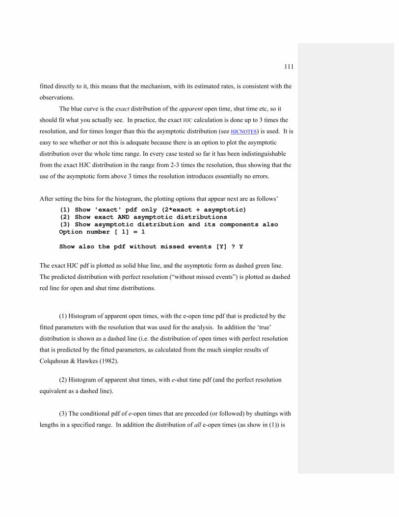
111

fitted directly to it, this means that the mechanism, with its estimated rates, is consistent with the

observations.

The blue curve is the exact distribution of the apparent open time, shut time etc, so it

should fit what you actually see. In practice, the exact HJC calculation is done up to 3 times the

resolution, and for times longer than this the asymptotic distribution (see HJCNOTES) is used. It is

easy to see whether or not this is adequate because there is an option to plot the asymptotic

distribution over the whole time range. In every case tested so far it has been indistinguishable

from the exact HJC distribution in the range from 2-3 times the resolution, thus showing that the

use of the asymptotic form above 3 times the resolution introduces essentially no errors.

After setting the bins for the histogram, the plotting options that appear next are as follows’ (1) Show 'exact' pdf only (2*exact + asymptotic) (2) Show exact AND asymptotic distributions (3) Show asymptotic distribution and its components also Option number [ 1] = 1 Show also the pdf without missed events [Y] ? Y

The exact HJC pdf is plotted as solid blue line, and the asymptotic form as dashed green line.

The predicted distribution with perfect resolution (“without missed events”) is plotted as dashed

red line for open and shut time distributions.

(1) Histogram of apparent open times, with the e-open time pdf that is predicted by the

fitted parameters with the resolution that was used for the analysis. In addition the ‘true’

distribution is shown as a dashed line (i.e. the distribution of open times with perfect resolution

that is predicted by the fitted parameters, as calculated from the much simpler results of

Colquhoun & Hawkes (1982).

(2) Histogram of apparent shut times, with e-shut time pdf (and the perfect resolution

equivalent as a dashed line).

(3) The conditional pdf of e-open times that are preceded (or followed) by shuttings with

lengths in a specified range. In addition the distribution of all e-open times (as show in (1)) is

112

superimposed as a dashed line. This display may be repeated for different shut time ranges. For

example, to look at distributions of apparent open times that are adjacent to short shut times,

specify a shut time range of, say, 0.025 to 0.1 ms. The dashed red line shows the unconditional

HJC distribution (for all shut times), for comparison.

(4) The mean open time for openings that are preceded (or followed) by shuttings with

lengths in a specified series of ranges (e.g. 0.05 to 0.15ms, 0.15 to 1ms, 1 to 10ms and 10 to

10000ms; you are asked for the number of ranges first, then for the lower and upper limits for

each range). Note that, for a useful comparison with data, ranges must be chosen that contain

reasonable numbers of shut periods. The observed mean open times (with standard deviation of

mean) are plotted against the mean length of the shuttings in each range (green at present, but see

screen and printout). The HJC values that are calculated from the fitted rate constants for the

same shut-time ranges (Colquhoun Hawkes & Srodzinski, 1996) are also plotted (blue at present,

but see screen and printout). The theoretical continuous relationship between mean open time

and previous or following shut time (red/yellow line at present) is also plotted, but this cannot be

observed directly.

The conditional distributions can all tend to 0/0 at high enough values of the adjacent

shut time. Once all exponentials but the slowest have decayed a limiting form of the

relationships in Colquhoun Hawkes & Srodzinski (1996) is used to calculate the plots (the results

are given below).

(5) The 3D distributions. The bivariate distribution of open time and adjacent shut time,

f(to, ts), (or of open times separated by specified lag) can be plotted. It is hard to make much of

this visually, so Magleby & Song (1992), suggested that the useful information in it could be

more helpfully plotted as a “dependency plot”. See also Colquhoun & Hawkes (1995) for a brief

account.

Dependency is defined as

1)()(

),(),(

ssoo

soso −=

tftfttf

ttd

where f(to, ts) is the bivariate pdf, as above, and fo(to) and fs(ts) are the normal unconditional open

time and shut time distributions, respectively. The dependency will therefore be zero if open and

113

shut times are independent, above zero if there is an excess of open times at any specified shut

time, and below zero if there is a deficiency.

The parameters for the histograms etc are set exactly as in EKDIST (see EKHELP.DOC).

All plotting is done with the same routines (VHIST or VPLOT) that are used in other

programs (see separate help notes, VPLOTHLP.DOC, for details of how to change colours, line

thickness etc, and how print or queue the plots).

(14) Save the fitted values of rate constants

After the fit, the calculated EC50 is printed out (this is done numerically, so unlike the

EC50 constraint, it should work whatever model you used).

After this has been printed, you are asked whether you want to save the fitted parameters

and if you say you do, then you are offered a default file name. Often it will be convenient to

crate a new QMECHS.MEC file with a name that suggests which fit it came form (e.g.

QDEMO.MEC). This will be a file identical with QMECHS.MEC but containing only one model, that

just fitted, and the fitted values of the rate constants. You can now use the fitted rate constants in

any of the theory programs by specifying its name when asked for the QMECHS file.

(15) Calculate standard deviations of, and correlations between, the fitted rate constants (see

below, and HJCNOTES.DOC).

After the plots are finished, you are asked whether you want the errors of the parameters

to be found (this is postponed until after plots gave been done in case the error calculation

crashes, though the present version has been very stable). The method for calculation of the

approximate standard deviations for each parameter estimate (and for correlations between

parameter estimates) is outlined in HJCNOTES.DOC. The calculations involve the numerical

estimation of partial second derivatives, and the accuracy of these depends on choice of a

suitable step size for each parameter. The default procedure is to look for an increment in each

parameter that reduces the log-likelihood by about 0.1 unit, and this seems satisfactory. If in

doubt, repeat the calculation with a larger or smaller step (the smaller the better as long as it is

114

not so small that the calculation suffers from rounding errors). The results should be

independent of the step size chosen.

Indeterminate parameters. It is, unfortunately, by no means uncommon for the value of

one or more rate constants to be poorly defined. This means that the likelihood is insensitive to

the value of that parameter, and a value of the second derivative that is needed for the

information matrix may be impossible to calculate. When this happens it becomes impossible to

invert the information matrix (see HJCNOTES.DOC). Rather than abandon the error calculations

altogether, we omit the row(s) and column(s) that correspond to indeterminate parameters from

the information matrix, and proceed to invert what is left. This procedure is an approximation (it

can be justified only if the off-diagonal elements are small enough), but it is likely to be a

reasonable approximation. In any case, standard deviations for parameter estimates that are

found in this way are almost always over-optimistic, in the sense that they indicate a smaller

amount of variability than is actually seen when the experiment is repeated several times.

After the error calculations, the correlation matrix is printed (see HJCNOTES.DOC), and the

parameter estimates are printed again, this time with their (approx) standard deviations, and

coefficient of variation (expressed as a percentage). The (first part of) a typical printout might

look like this

FINAL VALUES OF RATE CONSTANTS

Number of evaluations = 3163 Max log(likelihood) = 54600.1

Set 1: Agonist conc (micromolar) = 0.100000 Analysed in bursts, tcrit (ms) = 3.50000 Resolution (microsec) = 25.0000

initial final approx SD CV(%) 1 q( 1, 4)= alpha2 1500.00 1198.72 49.3282 4.11508 2 q( 4, 1)= beta2 50000.0 68849.5 1587.07 2.30512 3 q( 2, 5)= alpha1a 7000.00 2350.76 224.721 9.55949 4 q( 5, 2)= beta1a 60.0000 21.0282 2.78150 13.2275 5 q( 3, 6)= alpha1b 30000.0 37619.2 2444.26 6.49737 6 q( 6, 3)= beta1b 6.00000 152.090 13.5940 8.93813 7 q( 4, 6)= k(-2)b 1000.00 2508.85 not def (constrained) 8 q( 6, 4)= k(+2)b 0.100000E+09 0.682540E+09 0.637798E+08 9.34447 9 q( 4, 5)= k(-2)a 1000.00 752.371 not def (constrained) . . .

115

References

Colquhoun, D. & Hawkes, A. G. (1982). On the stochastic properties of bursts of single ion channel openings and of clusters of bursts. Philosophical Transactions of the Royal Society London B 300, 1-59.

Colquhoun, D. & Hawkes, A. G. (1995). The principles of the stochastic interpretation of ion channel mechanisms. In Single Channel Recording, eds. Sakmann, B. & Neher, E., pp. 397-482. Plenum Press, New York.

Colquhoun, D., Hawkes, A. G., & Srodzinski, K. (1996). Joint distributions of apparent open times and shut times of single ion channels and the maximum likelihood fitting of mechanisms. Philosophical Transactions of the Royal Society London A 354, 2555-2590.

Colquhoun, D. & Sakmann, B. (1981). Fluctuations in the microsecond time range of the current through single acetylcholine receptor ion channels. Nature 294, 464-466.

Colquhoun, D. & Sakmann, B. (1985). Fast events in single-channel currents activated by acetylcholine and its analogues at the frog muscle end-plate. Journal of Physiology (London) 369, 501-557.

Hawkes, A. G., Jalali, A., & Colquhoun, D. (1990). The distributions of the apparent open times and shut times in a single channel record when brief events can not be detected. Philosophical Transactions of the Royal Society London A 332, 511-538.

Hawkes, A. G., Jalali, A., & Colquhoun, D. (1992). Asymptotic distributions of apparent open times and shut times in a single channel record allowing for the omission of brief events. Philosophical Transactions of the Royal Society London B 337, 383-404.

Magleby, K. L. & Song, L. (1992). Dependency plots suggest the kinetic structure of ion channels. Proceedings of the Royal Society London B 249, 133-142.

Sakmann, B., Patlak, J., & Neher, E. (1980). Single acetylcholine-activated channels show burst-kinetics in presence of desensitizing concentrations of agonist. Nature 286, 71-73.

116

Wyllie, D., Béhé, P., Edmonds, B., Nassar, M., Schoepfer, R., & Colquhoun, D. (1996). Whole-cell and single-channel currents from recombinant NMDA NR1/2D receptors expressed in Xenopus oocytes. Journal of Physiology (London) 491, 135-136P.

117

\word_doc\HJCNOTES.DOC

MISSED EVENTS: A VERY BRIEF SUMMARY OF THE THEORY 1. Open and shut time distributions

2. Missed events: definition of e-open times

3. Distribution of the e-open times -what you actually see.

4. Calculation of the e-open time distribution 5. Fitting experimental records: the traditional method

6. Fitting experimental records: direct fitting of a mechanism to the whole sequence

7. What to do if the whole record is not from one channel

8. Determinacy of parameters: constraints and correlations

References

1. Open and shut time distributions

In the simplest case of a single open state (and no missed events) the probability density function (pdf) for the distribution of open times is a simple exponential distribution, viz

f(t) = τ −1 exp(−t/τ) (1.1)

where τ is the mean open time. In terms of the rate constant λ = 1/τ, this is

f(t) = λ exp(−λt) (1.2)

If there are several open and shut states, the open time pdf can still be written in a very similar way to that in (2), viz

f(t) = φA exp(QAA t) (−QAA) uA (1.3)

Although this is entirely general, and is valid for any mechanism, it does not look much different from the simple exponential in eq. (1.2), with the matrix −QAA in place of the λ in eq. (1.2). The only differences from eq. (1.2), apart from this, are the initial vector φA, which contains the

118

relative probabilities of an opening starting in each of the open states, and the final column vector, uA , with all elements unity, which has the effect of summing over all open states. When eq. 1.3 is appropriately expanded it turns out to be a mixture of kA exponentials.

In order to explain what QAA is, we may proceed as follows. Divide the total number of states, k say, into two subsets: set A contains the open states, kA in number, and set F contains the shut states, kF in number. The mechanism can be described by a Q matrix. The element in ith row and jth column of this table is denoted qij. The off-diagonal entries (i ≠ j) contain the transition rates (in s-1) for transition from state i to state j (or zero for states that are not connected). The diagonal entries (i = j) are then constructed so as to make the rows sum to zero; inspection of the example shows that the mean lifetime of state i is therefore −1/qii, because the diagonal elements, qii ,contain the sum of the rates for leaving state i.

As an example consider the usual nicotinic mechanism, with the states numbered as follows.

Scheme 1

The Q matrix is therefore

⎥⎥⎥⎥⎥⎥

⎦

⎤

⎢⎢⎢⎢⎢⎢

⎣

⎡

−++β−β

+β−βα+α−

α+α−

=

++

−−++

−−

−−

++

][2][2000)][(][0

02)2(000)2(200][])[(

11

112121

2222

2*

22*

2

1*

2*

21

AkAkkkAkAk

kkkk

AkAk

Q (1.4)

119

= ⎥⎦

⎤⎢⎣

⎡

FFA

AFAA

QQQQ

F

(1.5)

The dotted lines show the matrix partitioned into open and shut states. For example the submatrix QAA in this case is

QAA = ⎥⎦

⎤⎢⎣

⎡

+−+−

−−

++

)2(2]A[])A[(

*22

*2

*2

*21

kkkk

αα

(1.6)

This is an example of the matrix QAA that is used in eq. (1.3).

The open time pdf in eq. (1.3) can also be written in the form

f(t) = φA exp(QAA t) QAF uF

= φA GAF(t) uF (1.7)

where the matrix GAF(t) is defined as exp(QAA t) QAF. This matrix, with kA rows and kF columns

has elements gij(t) that give probability densities for staying open (i.e. in one or other of the open

states) for a time t, and then leaving for shut state number j, given that we started in open state

number i. The equilibrium initial vector φA gives the probabilities of starting in each of the open

states (i = 1 or i = 2 in the example, so φA = [φ1 φ2]); the value of φA can be calculated from the

Q matrix as the average fraction of openings that start in open state i in the steady state (the

equations assume the channels are in a steady state, not necessarily at equilibrium). The final

unit column vector (all elements = 1), uF, sums over the shut states (an opening is ended by entry

into any of the shut states). This example is explained in slightly more in the introductory

section of Colquhoun & Hawkes (1982, pp. 13-15).

2. Missed events: definition of e-open times

The aim is to derive the distribution of what is actually seen, rather than the distribution

of what would be seen if we had perfect resolution. In other words we want the distribution of

the observed or apparent open times (and shut times). In order to do this we must define

precisely what an observed open time means. Firstly we suppose that all events longer than

120

some specified resolution or dead-time, tres, are detected and measured accurately, but no events

shorter than tres are present (this is achieved by imposing a resolution in our programs, though not

in most others). The usual definition is an extended open time, or e -open time, which starts

when an opening longer than tres occurs, and continues until a shutting longer than tres is

encountered. The e-opening can therefore contain any number of shuttings, as long as they are

all shorter than tres, separating openings that may be of any length (except for the first, which

must be greater than tres). Note that this definition allows an e-opening to contain a succession of

consecutive short opens and gaps, possibly all less than tres, that might give rise to a wobbly

looking opening, or the false appearance of a sublevel, so this definition cannot in all respects

describe an 'observed opening' in the same way as if would be judged (subjectively) while fitting

real data. This definition of an observed opening (or shutting) is what is now implemented when

a fixed resolution is imposed on the single channel record in HJCFIT or EKDIST.

The extended shut time, or e-shut time, is defined in an exactly analogous way, as an

approximation to the observed, or apparent, shut times that are measured from real data.

3. Distribution of the e-open times -what you actually see.

By use of suitable notation, Hawkes, Jalali & Colquhoun (1990, 1992) make the pdf for

the e-open time, to, look no more complicated than that already given in (1.7), viz

f(to) = φA eGAF(to) uF (3.1)

The difference is that GAF(t) is replaced by an analogous matrix, eGAF(t), that is defined in a way

that allows for missed events (the 'e' appended to the symbol signifies extended times). This

simplicity disguises, of course, the fact that eGAF (t) is a good deal more complicated to calculate

than GAF(t). In a precisely analogous way the pdf for e-shut times, ts, can be written (e.g. simply

by exchanging A and F) as

f(ts) = φF eGFA(ts) uA (3.2)

121

4. Calculation of the e-open time distribution

Several approximate solutions to the problem have been proposed since e-openings were

defined, and the simplest 2-state case solved, in (Colquhoun & Sigworth, 1995). One of these

approximations is used in the only other program that does the same sort of fitting as HJCFIT,

namely QUB ((Qin et al., 1997) and http://barrel.med.buffalo.edu/) . However an exact solution

was found by (Hawkes et al., 1992;Hawkes et al., 1990) (the initial letters of the authors names

gave rise to the abbreviation HJC distributions). This solution is unusual in that it is piecewise;

the solution is different for the 1st, 2nd, . . . dead time. For example if the resolution (dead time)

is 25 µs then in the 1st dead time range, i.e. from 25 to 50 µs, the solution is a mixture of k−1

exponentials (but with the time constants that would appear in a noise, or relaxation analysis, the

eigenvalues of −Q, rather than the kA eigenvalues of QAA). In the 2nd dead time range, from 50

to 75 µs, the solution has the same exponentials but each is multiplied by a linear function of

time, and in the 3rd dead time range (75 to 100 µs) each exponential is multiplied by a quadratic

function of time. These polynomials of ever higher degree soon make the exact solution

numerically unstable so it is usable only for smallish times. However an approximation for large

times is given by Hawkes, Jalali & Colquhoun (1992), the asymptotic solution, and tests suggest

that it is necessary to use the exact solution only for the first two dead times, i.e. for intervals of

duration up to t = 3tres; thereafter the asymptotic form holds to an excellent approximation. The

really elegant thing about the asymptotic e-open time solution is that it has the form of a mixture

of kA exponentials, exactly as it would if no events were missed, though the time constants and

areas are, of course different when events are missed.

5. Fitting experimental records: the traditional method

Suppose that we have a series of alternating open and shut times (e.g. as fitted by the

SCAN program), thus

(5.1) open1: to1 = 2 ms

shut1: ts1 = 10 ms

open2: to2 = 5 ms

122

Fitting could be done separately for the apparent open and shut times, burst lengths and so on

This, however, tells us nothing directly about mechanisms. If we have no idea what kinetic

mechanism underlies the channel activity (which is usually the case) then it is all we can do, and

it does provide an empirical summary of what was observed. The procedure is based on the

premise that any Markovian mechanism will give rise to distributions that are the sum of

exponential (or geometric) components. When observed distributions are fitted with such

components (usually by the maximum likelihood criterion as done in the EKDIST program), we

maximise the likelihood for the time constants and areas for each distribution separately. This

works as follows, int the case of fitting the open time distribution..

For open times we have observed values of to1, to2, to3. . .. Denote the distribution of the

open times is denoted f(to); this might be a mixture of two exponential densities with time

constants τ1 and τ2, and areas a1 and a2 = 1− a1, thus

)/exp()/exp()( 2o1

221o1

11o ττττ tatatf −+−= −− (5.2)

Two components would be expected in the case of scheme 1, but in the absence of a specified

mechanism there is no reason to expect any particular number (criteria for the number to be fitted

are discussed by (Colquhoun & Sigworth, 1995)). the probability (density) of observing to1 and

to2 and to3 and . . .is usually taken as the product of the densities for each opening (though this is

not exact when open times are correlated, as is often the case). This is the likelihood of a the

particular parameters (τ1, τ2, a1) used to calculate it, and is given by

L = f(to1) f(to2) f(to3) . . . . (5.3)

The values for the parameters (τ1, τ2, a1) are adjusted to as to maximise this likelihood.

If we subsequently want to infer something about mechanism from the results, we are

faced with many different distributions that have to be synthesised into a consistent mechanism.

Often these distributions will contain overlapping information (for example the distribution of

burst length, and of total open time per burst, will be similar if shut times within bursts are

123

short). This synthesis may be far from easy. Furthermore, the conventional maximum

likelihood fits, used in EKDIST and other programs, assume that open times etc are independent of

each other, which is rarely true; usually they show correlations. If we want to fit a mechanism,

and have a candidate mechanism in mind, it will obviously be preferable to take a different

approach, and the optimum approach is described next.

6. Fitting experimental records: direct fitting of a mechanism to the whole sequence

We want to fulfil the following criteria.

(a) We want to fit as the free parameters the rate constants in the mechanism (i.e. the Q matrix),

not arbitrary time constants and areas foe each sort of distribution separately.

(b) We want to fit all the data simultaneously, rather than taking open and shut times separately.

(c) We want to take into account the order in which the openings and shuttings occur so information from the correlation between them can be taken into account properly. Horn & Lange (1983) described such a method, but it did not become really feasible in practice until it became possible to allow properly for the limited frequency response of real recordings ((Colquhoun et al., 1996), (Qin et al., 1997)).

In the case where there is only one channel contributing to the observed record this can be done very elegantly now that missed events can be taken into account at the time of fitting (it was not possible when, as up to now, corrections for missed events could be made only retrospectively). We simply calculate the likelihood as the probability (density) of the whole observed sequence of open and shut times, in the order in which they occur, as

L = φA eGAF(to1) eGFA(ts1) eGAF (to2) eGFA(ts2) eGAF(to3) . . . . uF .. (6.1)

This can be evaluated from the known resolution and the Q matrix, which specifies the mechanism, and the values of the rate constants in it. The parameters are not now the τ1, τ2, a1 , etc for arbitrary exponentials, but are the elements the Q matrix, i.e the rate constants in the mechanism. These rate constants are adjusted so as to maximise the likelihood in eq.6.1. This procedure not only takes into account both open and shut times but also takes into account their sequence: if there are correlations between open and shut times, as there are for nicotinic and NMDA receptors, then there will be information in the sequence and this method exploits it.

There are two ways to look at the result in eq. 6.1. One way is to look at is an enormous (matrix) product of probabilities (densities) that gives the joint probability of making all the observations. Another, rather nicer, way is to regard it as repeated calculation of the initial vector for each opening an shutting so that it has the appropriate values given the past history of

124

the record (the probability of entering each of the shut states, for example, will depend on what state the system was in at the time when that state is entered -e.g. ins scheme 1, if the previous opening was singly liganded, AR*, the next shutting must start in AR). From this point of view, notice that φA is a (1 × kA) vector that gives the probability that an opening starts in each of the open states at equilibrium, and when the next factor in eq. 6.1 is included, φA

eGAF (to1) is a (1 × kF) vector that gives the probability that the next shut period starts in each of the shut states following an opening of length to1; and φA

eGAF (to1) eGFA (ts1) is again a (1 × kA ) vector that gives the probability that the next opening starts in each of the open states following an opening of length t01 and a shutting of length ts1, and so on, up to the end of the data record.

7. What to do if the whole record is not from one channel

There are two slightly different methods for dealing with the problem that the

number of channels present is often not known. Both methods depend on dividing the observed record into groups of openings that are sufficiently short that we can be sure that all the openings in each group do come from one individual channel. Two cases can be distinguished by the following examples.

(1) At medium and high agonist concentrations there will often be sufficient desensitisation that long groups or clusters of openings, that are clearly separated by longer silent periods during which all channels in the patch are desensitised, as first observed by (Sakmann et al., 1980). The probability of the channel being open during each such group may be high enough that we can be confident that the whole group comes for on individual channel if no double openings are seen (Colquhoun & Ogden, 1988; Colquhoun & Hawkes, 1990).

(2) In steady state records measured at low agonist concentrations, the number of

channels that are present will never be known. In this case the best that can be done is to suppose that all the openings in single activations of the channel come from the same individual channel. For example (Colquhoun & Sakmann, 1985) exploited the fact that all the (1-10 or so) openings in a burst (single activation) of the nicotinic receptor were almost certainly from the same channel. The shut times within such bursts can be predicted by the model, but not the shut times between burst.

In either case, groups of openings must be defined in the experimental record by

specifying an appropriate critical shut time, tcrit, such that all openings that are separated by shut times less than tcrit can be assumed to come from one individual channel. What we do next depends on whether or not the long shut times (longer than tcrit) that separate groups are spent in states that are included in the kinetic mechanism that is being fitted. For example, in case (2) it might be assumed that there is very little desensitisation, so a mechanism like scheme (1) would be an adequate description of all the states. However in the first example above, this would be true only if desensitised states were added to scheme (1). If we used scheme (1) without adding desensitised states to it, then the best that could be done is to calculate the likelihood separately, using eq. 6.1, for each group of openings. We then multiply together the likelihoods for each of the groups to obtain a final likelihood for all of the observation, and that is what is maximised. Strictly speaking the initial and end vectors would not be correct because each group of openings starts from, and exits into, shut states that are not included in the mechanism. However this is

125

not likely to matter much in practice because the groups of openings obtained in such experiments are usually quite long (contain many open and shut times)so the initial and final vectors do not affect the answer much.

However we can do a little better in the cases where the specified reaction mechanism does contain all the states present in the data. The length of the shut time that precedes the first opening in a group is not known precisely, but it is known to be greater than tcrit. The probability that the first opening in a group begins in open state i (state 1 or 2 in the example above) must take account of this knowledge, rather than supposing (as the equilibrium φA used above does) that it could be any length. Likewise the shutting that follows the last opening of a group is known to be longer than tcrit, though how much longer is unsure. We thus can define a likelihood for the rth group, with n openings in it, as

Lr = φb eGAF (to1) eGFA (ts1) eGAF (to2) eGFA (ts2) . . . . eGAF (ton) eF , (7.1)

where the initial and final vectors, φb and eF , are now those appropriate to the specified tcrit value. These can be defined, not by the method of defining bursts in terms of a subset of short-lived shut states (as in Colquhoun & Hawkes, 1982), but directly from the specified tcrit value. Thus the (kF × 1) column vector at the end does not have all entries = 1 (uF) as in eq.(6.1), but rather is (Colquhoun et al., 1996)

∫∞

=crit

d)(t

AFAe

F tt uGe . (7.2)

This simply specifies that after the last opening of the group one of the shut states is entered and the channel remains within the shut (F) states for any time from tcrit to ∞, before eventually reopening. The initial vector φb can be defined along the same lines. + Once tcrit is specified the observed record can be divided up in N groups and the likelihood for each group can be calculated from eqs.7.1 and 7.2. The final likelihood, which is to be maximised is then the product of the likelihoods for each group.

L = L1 L2 L3 . . . LN (7.3)

In practice the record is almost always broken up into groups anyway, because the analysis of the raw data in SCAN will usually have labelled some of the shut times as being unusable. This is done if, for example, an occasional double opening has to be excluded from the analysis, or if the patch temporarily becomes noisy. It is important that such events should be labelled because HJCFIT requires that events are in the actual order in which they occur.

8. Determinacy of parameters: constraints and correlations

It will often be the case that the data contain insufficient information to determine values for all of the rate constants in the mechanism. For example, if the data are not all from one

126

channel, and have to be fitted one activation at a time, there will be essentially no information about the association rate constants for binding of agonist. In this case it will be necessary to either fix the association rate constants at plausible values, or to constrain them so that the results conform to an EC50 values that is specified on the basis of independent experiments (see HJCFIT notes, hjchelp.doc, for more details). The number of parameters to be estimated can also be reduced if some constraints can be incorporated. For example, in scheme 1, if it were justified to assume that there order of binding were irrelevant (no inherent cooperativity in binding to shut channels) then k+1 = 2 k+2, and k−2 = 2 k−1 so the number of parameters to be estimated is reduced by two (see HJCFIT notes, HJCHELP.DOC, for more details). The errors in the fitted parameters can be found by calculation of the covariance matrix. An idea of how precisely a parameter is determined can be found by looking at how sharply the peak of the likelihood surface (see Fig 1) is defined. If the peak of the hill is very flat, this means that the value of a parameter can be moved quite a long way from the peak (maximum likelihood value) without causing a very big decrease in L, i.e. without causing the fit to become much worse. This means that the value of this parameter is not very well-defined by the data. On the other hand, if the hill as steep sides, even a small change in a parameter value will cause the fit to become much worse, and the value of that parameter is well-defined by the data. This is illustrated in Figure 1, which shows a range of values for the opening and shutting rate constants (like α2 and β2 in scheme 1). For each pair of α2 and β2 values, the corresponding log(likelihood) is plotted on the vertical axis. There were, of course, other free parameters in the fit, but to reduce the problem to only 3 dimensions, these were all fixed at their maximum likelihood values.

The rate at which the slope changes near the maximum in this surface gives a measure of the curvature (‘non-flatness’) of the top of the hill. The rate of change of slope is measured by the second derivative, so it makes sense that the observed information matrix is defined, in general, thus.

127

⎥⎥⎦

⎤

⎢⎢⎣

⎡−=

=

−

θθ∂θ∂θ

∂

ˆ

21

ji

LV , (8.1)

where θ represents the array of parameters, and L is the log-likelihood defined above. The subscript indicates that this is evaluated at the minimum, the point at which we are interested in the curvature. If there were no correlation between the parameter estimates, all the off-diagonal elements would be zero, and the diagonal elements would the reciprocals of the variances of the estimates, so inversion of (17) would give variances for the parameter estimates. More generally, inversion of (17) gives the covariance matrix, V, the diagonal elements of which are variances of the parameter estimates, and the off-diagonal estimates are their covariances. The latter are usually presented as correlation coefficients, r, found for the covariances via the relationship

)(var)var() ,cov(

),(21

2121 θrθ

θθθθr = (8.2)

The HJCFIT program makes a numerical estimate of (17) and uses it to calculate approximate standard deviations for the estimates (as square roots of the diagonal elements of the covariance matrix), and the correlation matrix.

It has been found while fitting mechanisms like that in scheme (1) that there is often a strong correlation between α2 and β2, with r(α2 , β2) = -0.85 to 0.99. This is seen graphically as the diagonal ridge in Figure 1. This ridge shows that the fit does not get much worse (L does not decrease much) when α2 is increase if β2 is also increased. This has a simple physical meaning. Increasing α2 means that individual openings are shorter, but increasing β2 means that more re-openings occur. The correlation means that it is not easy to tell whether the observed apparent openings consist of many short openings, or fewer longer openings.

The fact that α2 and β2 are positively correlated also means that their ratio, the efficay E2 , is better defined than the separate rate constants.

128

The existence of the ridge in Figure 1 can also slow down the fitting process. The values of α2 and β2 tend to increase and decrease in parallel as simplex tries to crawl along the ridge. The progress of a fit in which the correlation was very high (0.99) is shown in Figure 2

Progress from the initial guess at the bottom is initially rapid, but then both α2 and β2 increase in parallel before coming back down the ridge, both decreasing, to reach a maximum (many points have been omitted for clarity).

References

129

Colquhoun, D. & Hawkes, A. G. (1982). On the stochastic properties of bursts of single ion

channel openings and of clusters of bursts. Philosophical Transactions of the Royal Society

London B 300, 1-59.

Colquhoun, D. & Hawkes, A. G. (1990). Stochastic properties of ion channel openings and

bursts in a membrane patch that contains two channels: evidence concerning the number of

channels present when a record containing only single openings is observed. Proceedings of the

Royal Society London B 240, 453-477.

Colquhoun, D., Hawkes, A. G., & Srodzinski, K. (1996). Joint distributions of apparent open

times and shut times of single ion channels and the maximum likelihood fitting of mechanisms.

Philosophical Transactions of the Royal Society London A 354, 2555-2590.

Colquhoun, D. & Ogden, D. C. (1988). Activation of ion channels in the frog end-plate by high

concentrations of acetylcholine. Journal of Physiology (London) 395, 131-159.

Colquhoun, D. & Sakmann, B. (1985). Fast events in single-channel currents activated by

acetylcholine and its analogues at the frog muscle end-plate. Journal of Physiology (London)

369, 501-557.

Colquhoun, D. & Sigworth, F. J. (1995). Fitting and statistical analysis of single-channel records.

In Single Channel Recording, eds. Sakmann, B. & Neher, E., pp. 483-587. Plenum Press, New

York.

Hawkes, A. G., Jalali, A., & Colquhoun, D. (1990). The distributions of the apparent open times

and shut times in a single channel record when brief events can not be detected. Philosophical

Transactions of the Royal Society London A 332, 511-538.

130

Hawkes, A. G., Jalali, A., & Colquhoun, D. (1992). Asymptotic distributions of apparent open

times and shut times in a single channel record allowing for the omission of brief events.

Philosophical Transactions of the Royal Society London B 337, 383-404.

Horn, R. & Lange, K. (1983). Estimating kinetic constants from single channel data. Biophysical

Journal 43, 207-223.

Qin, F., Auerbach, A., & Sachs, F. (1997). Maximum likelihood estimation of aggregated

Markov processes. Proceeding s of the Royal Society London B 264, 375-383.

Sakmann, B., Patlak, J., & Neher, E. (1980). Single acetylcholine-activated channels show burst-

kinetics in presence of desensitizing concentrations of agonist. Nature 286, 71-73.

131

The limiting form of the conditional mean open time for large adjacent shut times

The expressions derived below are used to calculate conditional distributions (plot types 3 and 4) in HJCFIT when the ‘adjacent shut time’ is so large that the conventional expressions tend to 0/0. (1) Theoretical continuous form The theoretical continuous form of this relationship is given by eq 3.5 in Colquhoun Hawkes & Srodzinski (1996) (referred to as CHS96 below). Because it is a missed-event (HJC) distribution it looks quite complicated.

AFAe

F

FFFAFs

AFA

eF

cot

dssdt

tTTEuGφ

uQQRGφ

)(

)exp()()(

)(1

0

*1

1

ξ

ξ =⎥⎥⎦

⎤

⎢⎢⎣

⎡

+== ,

(3.5) where the denominator is the HJC shut time p.d.f., fTc(t1), and ξ is the resolution. The denominator must obviously, like any p.d.f., tend to zero as the shut time, t1, increases. The numerator also tends to zero. In both numerator and denominator, the only function of time is eGFA(t), and this is given by (see CHS eq 2.13)

)exp()()( ξξ AAFAF

FAe tt QQRG −= where R(t) is the ‘survivor function’. Since we are interested only in large times, this survivor function can be written (see 2.28) in its HJC asymptotic form as a sum of kF exponentials, the time constants of which are the HJC time constants for the asymptotic shut time distribution.

)/)(exp()(1

i

k

ii

FF ttF

τξξ −−=− ∑=

RR ,

where FRi are constant matrices. Thus the only function of time in (3.5) is this sum of exponentials. As time increases, these all tend to zero, but the terms with the fastest time constants declining fastest. The last term to vanish is that with the slowest time constant, τslow say. As time increases, eventually all terms but this slowest one become negligible. In fact, in the numerical calculations it is not possible to calculate a number smaller than exp(−708), so when the exponent gets below –708 the exponential gets set to zero exactly, to prevent floating underflow; thus as time increases the only non-zero term left is the slowest. When there is only one exponential in the sum, then

132

)/)(exp()( slowslowFF tt τξξ −−≈− RR

Now exp(−(t−ξ)/τslow) is a scalar multiplier in both numerator and denominator and so it can be cancelled. Thus the limiting form can be calculated by using the constant FRslow in place of FR(t−ξ) in both numerator and denominator, i.e. by replacing eGFA(t) in (3.5) by

)exp( ξAAFAslowF QQR (2) Mean open time conditional on adjacent shut time being within specified range This is given by eq 4.8 in CHS96

)()()exp()]()([)(

loThiT

FAFAAFAloF

hiF

Fhicloo tFtF

tttTtTEcc

−−−−

+=<<uZQQKKφ ξξξξ

4.8 where ZAF stands for the product of several constant matrices (see original). The cumulative matrices in the numerator are defined in CHS96, eq. 4.4, for large times as

∑=

−− −+=F

iik

i

uii

FFF u1

//2 )ee()2()( ττξτξ RKK , u > 2ξ,

where u ≡ t – ξ is the ‘excess time. Much of this is constant, and subtracts out when the difference between two K matrices is found in the numerator of 4.8. This part can be written as

∑=

−− −=−−−F

ihiilok

i

uuii

Flo

Fhi

F tt1

// )ee()]()([ τττξξ RKK

The denominator of 4.8 can be written (for large t), using CHS eq.4.5 and 4.4, as AAAFAlo

Fhi

FFloThiT tttFtF

ccuQQKKφ )exp()]()([)()( ξξξ −−−=−

AAAFA

k

i

uuii

FF

Fihiilo uQQRφ )exp(])ee([

1

// ξτ ττ∑=

−− −=

When all exponentials in the sum have decayed to zero apart from the slowest, that with τslow , we are left with

)/)(exp()( slowslowFF tt τξξ −−≈− RR .

In this case both numerator and denominator contain the same scalar factor,

133

)ee( // slowhislowlo uu

slowτττ −− − ,

which can therefore be cancelled leaving the limiting value of the conditional mean open time, (4.8) as

FAAFAslowF

F

FAFAAFAslowF

Fhicloo tTtTE

uQQRφuZQQRφ

)exp()exp()(limξ

ξξ +=<<

(3) Mean shut time within a specified range This is the x value against which the conditional mean open time in para (2) is plotted From CHS96. eq. 4.9 it is

)()()exp()]()([)(

loThiT

FAAFAloF

hiF

Fhicloc tFtF

tttTtTEcc

−−−−

+=<<uQQMMφ ξξξξ , (4.9)

where, for large t, M is given by CHS96, eq. 4.11,

∑=

−− +−++=F

iik

i

uiiii

FFF uu1

//2 ]e)(e)2[()2()( ττξ τξττξ RMM . u > 2ξ,

where u ≡ t – ξ is the ‘excess time. Thus the difference between two such terms, as in the numerator of (4.9), is

∑=

τ−τ− +τ−+ττ=ξ−−ξ−F

ihiilo

k

i

uhii

uloiii

Flo

Fhi

F uutt1

// ]e)(e)[()]()([ RMM

The denominator is the same as in para (2), so when all exponentials but the slowest (with time constant τs) have decayed we get

FAAFAuu

ssF

F

FAAFAu

hisu

losssF

Fhicloc shislo

shislo uutTtTEuQQRφ

uQQRφ)exp(]ee[[

)exp(]e)(e)[()( //

//

ξ−τξ+τ−+ττ

+ξ=<< τ−τ−

τ−τ−

.

Taking out the scalar multipliers this becomes

⎟⎟⎠

⎞⎜⎜⎝

⎛−τ

+τ−+ττξξ

+ξ=<< τ−τ−

τ−τ−

]ee[]e)(e)[(

)exp()exp()( //

//

shislo

shislo

uus

puhis

uloss

FAAFAsF

F

FAAFAsF

Fhicloc

uutTtTEuQQRφuQQRφ

The matrix expressions are scalar and so can be cancelled giving

134

⎟⎟⎠

⎞⎜⎜⎝

⎛−τ

+τ−+ττ+ξ=<< τ−τ−

τ−τ−

]ee[]e)(e)[()( //

//

shislo

shislo

uus

puhis

uloss

hiclocuutTtTE

⎟⎟⎠

⎞⎜⎜⎝

⎛−

+τ−+τ+ξ= τ−−

τ−−

puu

puuhislos

slohi

slohiuu/)(

/)(

e1]e)()(

and for large times this is,

losloshicloc tutTtTE +=++=<< ττξ )()( Not surprisingly, the result has simplified to the mean of values greater than tlo for a the simple exponential distribution, f(t) = 1/τs exp(-t/τs), i.e.

los

t

t tttf

tttf

lo

lo +=

∫

∫∞

∞

τd)(

d)(

DC 17-May-02

135

CJUMP AND CJFIT PROGRAMS

All programs run with the 1401-plus interface. Note that when the computer is booted errors may be reported from the 1401. These errors are usually not real but result from having apparatus (especially switched-off apparatus) on the DAC and ADC connectors which impose a big capacitative load. When these are disconnected the 'errors' go away. (A) CJUMP To do concentration jumps and/or V-jumps and/or V-ramps on line. (1) Input/output. Current is recorded on ADC0 and, in the case of V-ramps only at present, voltage is recorded on ADC1. The signal for the C-jump piezo is on DAC2, and the membrane potential command signal is on DAC3. The outputs from the 1401 are undefined before switching it on, and can do odd things (e.g. oscillate) after switching it off. Therefore always switch the 1401 on first (and run the program to set the holding potential), and switch of piezo power supply before switching off 1401. (2) Triggering The ADC sampling is triggered through event 4, and DAC output through event 3, so these should be connected together so they are triggered simultaneously (there is also an option to trigger from keyboard, which issues an instruction to trigger E3 and E4 via software when <ENTER> is hit). The best way is to make a small box that can be triggered by a push-button to deliver a negative-going trigger to E3, E4 (the same trigger pulse can also be used to trigger a scope). (3) Running (a) Choose name for the data file and print file (b) Choose the disc partition where the data file (until recently CJUMP.DAT, but default name now CJUMP.CJD) will be written. Nothing is actually written to disc unless RECORD is on (the default is to have it on from the start, but you are asked whether you want it OFF initially). You can append data to an existing file, or overwrite an existing one. Too much data in one file can be confusing (especially if you don't put titles in). Make sure that there is room on the disc (files can get big). Rename old CJUMP.CJD files, or copy them to backup device, if you want to keep them (see BACKUP notes for details). The easiest way to check what's in an existing file is to run CJFIT and use the option to list all the titles in the file (scroll lock on to print them). (c) Give patch number, temperature, patch type, filter setting (d) Read parameters from disc?. Sets of parameters can be stored, once they have been defined in a file (the current version of the file is named CJUMP4.SPR), and the stored parameters can be read in at this stage. If you say NO then you are asked for all details of

136

gains, C-jumps and V-jumps, and ADC sample, and details of which of the sampled points are to be kept on the disc (simplest to keep all of them if you have a big enough hard disc). You must specify the following. (i) The DAC frequency; this is normally 1 kHz = 1 ms resolution, unless you want very long DAC pulses (use 0.1 kHz, 10 ms resolution), or very short (e.g. short gap before 1st jump) (for which use 10 kHz, 0.1 ms resolution). (ii) Duration of ADC sample; voltage to apply to piezo (max=5000mV, may need amplification externally) (iii) Details of c-jump protocol; gain for voltage command signal on DAC3 (Vcommand/V membrane pot). (iv) Holding potential. (v) Details of V-jump/ramp protocol (iv) ADC sampling frequency. Finally the number of points per ADC sample is given for approval. Once the sweep protocol is defined, the parameters can be saved (see below) and can be read back here by specifying set number. The parameters are typed for approval, and can be used as they are, modified or rejected. When several sets have been saved it is useful to make a printed version of what they are: easiest way is to put Scroll Lock on while reading in each set, so they are printed straight away (they are not put in the print-to-disc file).

After a new set of parameters is read from disc (at start, or, via key 7 during the experiment) you are asked whether you want (1) to use them as they are (default) (2) modify the multiple sweep details (see next para) (3) modify which points are to be kept on disc (4) modify all values (this goes through all questions; as when protocol not read from disc except that the values read come up as defaults) (5) read a different set. If you want to change only one or two things (e.g. c-jump length) it is easier to accept the protocol from disc as it is, but then alter the c-jump length once the menu boxes appear (e.g. with special jump-length key if it has been requested, or via C-JUMP protocol key on 2nd-level menu).

If, in CJUMP, you ask to modify which points are kept on disc, then if multiple sweeps are being done you can opt to keep the same points for each sweep, to keep sections of points that are in the same position relative to the c-jumps or v-jumps (which may change in position from one sweep to next), or to specify separately for every sweep exactly which points are to be kept (and whether to keep points at reduced frequency between the specified 'high resolution' sections). (e) Multiple sweeps. This option allows a specified sweep to be repeated several times, with a specified number of seconds between each sweep. When the number of sweeps is specified as 1, then the program functions as before. (At present the program downloads all parameters to the 1401 between each sweep, and displays the response between each sweep; the time taken for this means that the minimum time between sweeps is of the order of 400ms + sweep length; a warning is given if the time between sweeps is too short to do all these jobs.)

If the number of sweeps is greater than 1 then you have the option to change a single parameter between one sweep and the next. At present the options are (i) all sweeps the same (ii) change potential of voltage jump (iii) change duration of a c-jump (or of all c-jumps if more than one done per sweep), (iv) change length of the interval

137

between a pair of c-jumps done in a single sweep (the length of the first and second jumps are set to any required value in the ordinary way). If a multiple sweep protocol is read from the disc you get an extra option; viz to modify only the multiple sweep part of the protocol, i.e. the individual sweeps remain as specified but the number of sweeps, the interval between them, or the values that are changed from one sweep to the next, can be altered.

If a multiple sweep protocol is chosen you will be asked if you want to RANDOMISE the order of the sweeps (unless 'all sweeps the same' was chosen). If you say YES then a random permutation of n (the number of sweeps) is chosen; if the same multiple sweep protocol is run again then a new randomisation is done for each run. Pressing ESC will abort the series of sweeps, and print a message to that effect in print out, just as it will abort a single sweep while waiting for trigger (see para e, below). (f) After the protocol is defined you are asked about the gain for the ADC sample: calibration =10mV/pA, Gain=10 O.K. [Y] ? (or whatever values of calibration and amplifier gain have been read from disc). Just hit enter if this is correct, otherwise say N when you will be presented with the normal questions to define the calibration (N.B. do not say 'gain not to be specified here' because this sets the calibration factor to -1.0, as a signal that it hasn't been set yet, and will appear to reverse the direction of all currents!). Also specify gain for V-recording (mV out from clamp/mV membrane pot). Next you are asked what options to use for the special keys, as follows. (g) A title for the sample is requested, which goes onto disc (while recording) an helps to identify it. If the protocol was read from disc, the title comes up with the protocol title (if defined when saving protocol -see below) already in it (to save typing), and the title can be edited with home/end/left arrow/right arrow/backspace and DEL keys (when in graphics mode the cursor is not visible so editing is harder). (h) A graph appears (with no data the first time, when number averaged appears as zero), with boxes that control what is done next. Normally the next thing will be to do a jump. Hit key 1 or 2 on the main menu to do a jump (or any of the other keys for options specified next).

After the jump, a display of current vs time, for whole sweep, is shown. Vertical scale is whole 1401 range (-5 to +5 V at input). Zero line is dark blue, current sweep is green; mean of all sweeps (since last NEW MEAN) is red. Bars show the position of c-jump(s) (white), and v-jumps/ramps (yellow). At top title is shown, followed by the number of traces averaged. At top right a message shows whether data is being recorded on disc. Boxes at bottom of display ( the Main, or 1st level, menu) again give various options. Main (1st level) menu options

KEYS 1 and 2 (AGONIST and CONTROL JUMPS). Normally key 1 is used to do the

jump. If V-jumps/ramps are being done then hit key 1 (AGONIST JUMP) to do jumps in

agonist, or key 2 to do CONTROL JUMP (no agonist) jump. Key 2 causes V-jump/ramp

138

to be done without activating the piezo, and keeps the jump, and average jump, for

controls separate from those in agonist.

If you specified external trigger, a message appears saying 'waiting for external trigger . . .' , and the system is hung until trigger is received. If ESC key is hit at this point, instead of triggering, the jump is not done (and a message JUMP ABORTED appears on screen, and in the print-out), and the options boxes appear again to choose what to do next.

If keyboard trigger was requested, then the jump is done as soon as the AGONIST JUMP or CONTROL JUMP key is hit.

To do another jump hit key 1 (or 2, as above). It may be useful, especially for setting up, not to have to hit the keyboard (key 1 or 2) before each jump, so you can enter AUTO MODE (key 3). Key 3: 'AUTO MODE'. In this mode each press of the trigger produces a jump (agonist or control, whichever was in force when auto-mode entered). In this case there is no access to the options boxes, until auto mode is left by hitting ESC key while waiting for trigger. If RECORD was off at the time AUTO-MODE was entered it stays off, but a menu box (0. RECORD SWEEP) appears which allows the sweep that has just appeared on the screen to be recorded on disc (the same as when the special key option 6 is requested). KEY 4: 'NEW TITLE' allows a title to be attached to the jump, as well as the number averaged. This is very useful for keeping track of what's what when analysing the results later. KEY 5: 'NEW MEAN' starts a new average (for both agonist and control if V-jumps/ramps being done). A new average is also started automatically whenever the parameters are changed (sample rate, length, C- or V-jump protocol, holding pot or jump pot). KEY 6: 'RECORD' starts/stops recording of the data on disc (in CJUMP.DAT). Each individual jump is recorded, and in addition the current means are recorded (if they are means of more than one jump) whenever a new average is started (either with key 5, or automatically when parameters changed). Note that nothing is recorded until requested, but option now provided to switch recording on from start -this prevents forgetting to switch it on (hard experience!), but is only usable if you have everything pretty well set up, ready to go. While recording the number of the recorded trace appears on the screen (below 'Recording'), and can be noted as an aid to keeping track later. KEY 7: 'SHOW PARAMS'. This (i) types out the current set of parameters on the screen KEY 8: 'SHOW V-JUMP' This option allows the V-jump or V-ramp to be displayed at any time. The default option is to use the current mean agonist and control records, but the option is given to read specified earlier records from the disc for display. Then the

139

option is given either to show the V-jumps/ramps (unsubtracted or net), or to simply show voltage vs time for the whole sweep (if the sweep has a single V-ramp then short brown bars are drawn to indicate the voltages that the ramp should attain if voltage is well-controlled). The net I/V curves are calculated by the crude method (see CJFIT notes). If more than one jump/ramp is done during a sweep you will be asked which one to display. Jumps are shown as current vs time, and ramps are shown as I/V plots. In each case the agonist trace is red, the control trace is light blue and the net (difference) trace is yellow (if both agonist and control have not yet been done, only the one that has been done is displayed). KEYS 9 :'CALIBRATION' allows CALIBRATION to be altered (e.g. if you change mV/pA, amplifier gain etc; if you forget to change it here the calibration can be given in CJFIT, as long as you know the right values!). KEY 10: 'CJUMP LENGTH' changes the cjump length KEY -: 'PIEZO VOLTS' allows the voltage for piezo to be changed KEY +: MORE takes the user to the second level menu. KEY *: 'READ PARAMETERS' allows a new set of parameters to be READ from the disc. KEY /: 'SAVE PARAMETERS' allows the current parameters to be SAVED on the disc (overwriting an existing set if you want); when saving you are asked whether you want to give the protocol a short title (e.g. 'Gap series 10=500ms:', or 'V-ramp 3 sec:') -if given this will automatically appear in the sweep title in order to save typing when giving titles. KEY .: 'EXIT' exits the program. 2nd level menu options

KEY 1: 'HOLDING POTENTIAL' allows holding potential to be altered KEYS 2, 3 and 4 of the 2nd level menu allow change, respectively, of ADC sample rate and length, C-jump protocol and V-jump protocol; if, for example, a c-jump shorter than 1 ms is requested then the DAC output rate will be (re)set to 10kHz (0.1ms/point) (if a very long v-jump were being requested at the same time this could make the DAC array too long, but the program will tell you if so). KEY 5 toggles between External Trigger and Keyboard Trigger. KEY 6: 'JUMP POTENTIAL' allows jump potential to be altered

140

KEY 7: 'PRINT NOTE' asks for a note to be typed in (it can be edited as above) and this note is printed on the print-out (not in CJUMP.DAT) -useful, for example, to say 'gain was set wrongly in last 6 sweeps' (more hard experience). KEY 9: 'SWEEPS' redefine number of sweeps. KEY 10: 'MAIN MENU' takes the user back to main Menu KEY . 'EXIT PROGRAM' exits the program Permananent Data Storage

Experience shows that you will want to keep the original CJUMP.DAT data files, rather than relying on analyses and plots done during CJFIT. At the end of the experiment copy them to, say, disc L:\ and rename them at the same time, e.g. as CJUMP1.DAT, CJUMP2.DAT etc. (CJFIT can read these). Also copy to back-up floppies (they usually seem to fit on a floppy). The periodic mag tape backups should provide additional security. Plotting raw data

AUTPLOT has option to plot the raw current records from an entire CJUMP.CJD (CJUMP.DAT) file automatically, e.g., 4 per page (for 'speed'), without having to fit them first. This gives a nice record of the experiment for C-jumps (but is not much use for V-jumps or ramps for which the unsubtracted current records are not very informative.

141

(B) CJFIT PROGRAM

This program can re-do averages of records produced by CJUMP, and fit the results. At present averaged jumps can be fitted with rise time/peak or sums of exponentials, and I/V curves can be fitted with various functions (as in CVFIT). The input is the file produced by CJUMP (default file name CJUMP.CJD), but other options for the input to CJFIT are now available, thus. (1) Take data from CJUMP program (CJUMP.CJD) (2) Import data from MathCad (MCDAT.DAT) (3) Take data for fitting from plot queue(s) (PLOTQ.PLQ) (4) Average aligned bursts from CONSAM.SSD Option number [1] = The first option is the main, and original, version. The third option was added primarily to allow re-fitting of averaged relaxations, to avoid having to re-do the averaging. The only way to store such an average is to queue the plot, and this option allows a queued relaxation to be read in. The fourth option allows steady state data that have been fitted in SCAN to be read in, and bursts of openings to be read in Overwritten files

If the option to overwrite an existing CJUMP.CJD file was chosen in CJUMP then the new sweeps are added to the file starting at the beginning. However if the new experiment has generates fewer data than the one being overwritten, the size of CJUMP.CJD will stay as it originally was, and will still contain results from the original experiment that have not yet been overwritten (though the index to where they are has been overwritten). If the CJUMP.CJD is bigger than expected from the indexed (latest) sweeps then you will be told at this stage, and offered 3 options. (1) Leave the file as it is (this does no harm but wastes disc space). (2) To truncate the file to remove data from the earlier (partially overwritten) experiment from it, so the file now occupies less disc space (use this as long as you overwrote the earlier file on purpose and do not need to recover it). (3) To recover data from the older experiment that has not yet been overwritten by the newer (use this if you overwrote by accident!). This option starts with the last sweep it knows about, and searches through any subsequent records until it finds a valid file header (the date contains '199' for the 1st 3 characters of the year). If one is found then the space it occupies is calculated and the next sweep found. The results of this are not kept on the disk, so if you want to use any of these 'recovered' sweeps you must run this search each time the program is started. You can now either specify (1) which records to fit (either an individual jump, or the mean jump written to disc by CJUMP), or (2) you can go through the individual jumps to form a new average for fitting (this allows inspection of the records before they go into average, unlike in CJUMP). When records are taken straight from CJUMP you can specify a single record number to be fitted, or two record numbers (e.g. agonist and

142

control) the difference between which is to be fitted. Similarly when the sweeps are re-averaged you can make a single average, or two different ones (e.g. agonist and control). There are also options to (3) fit the next single sweep, or (4) fit the next single sweep using the same graph scaling/interpolation as the last (faster as long as the interesting area of each graph is the same), or (5) to SUPERIMPOSE up to 10 sweeps. The default answer to this question, as with several others in CJFIT, is 'learned' by the program; e.g. if you ask for option '(3) fit next single jump' once, then this option comes up as the default next time. The option to superimpose plots is rather rudimentary at present. It was written to superimpose a series of sweeps at different potentials, or a series of double pulse sweeps with different delays between pulses. It works only for current versus time sweeps, and no fitting is allowed at present. You specify the number of sweeps to be superimposed, and then which sweeps they are (not necessarily contiguous numbers). Then the option is offered to normalise all sweeps to the same baseline (e.g. for sweeps at different potentials) and, if this is requested, then you are asked for the times (ms from start of sample) between which the baseline is to be averaged to calculate the necessary vertical offset to line them up (e.g. if the jump starts at 50 ms from the start of the sample then you might use the bit from 25 to 45 ms to line them up). (3) Once the records to be fitted have been defined, you can specify the calibration here, if it was set wrongly in CJUMP (so this wrong value is read from the disc). If you change the calibration then for subsequent records you will be asked if you want to use the same corrected calibration again (default =Y), so you do not have to keep typing in the same correction. If you say No then the program reverts to reading the calibration from the disc. (4) The chosen records are displayed, the display options depend on the sort of experiment that was done. If a single record was fitted the display shows current vs time, I(t) vs t, with option to show voltage vs time (V(t) vs t) if voltage was recorded (V-ramps). If two records are specified you can show (1) I(t) vs t for both records (the whole record); (2) I(t) vs t for a specified V-jump only (if more than one V-jump done) or I/V plot for both records (for V-ramps); (3) The difference between the 2 records displayed in option 2, i.e. the net jump or net I/V curve; or (4) V(t) vs t for (the whole of) both records (in the case of a single voltage ramp, dashed lines show the potentials that the ramp should reach, as a quick check). If records with more than 2048 points are displayed then initially points are skipped so that no more than 2048 are put on screen. All points can be plotted by hitting POSH OPTION, SYMBOLS/LINES, ALL POINTS, i.e. KEYS 5, 6, 7 (repeat to revert to omission of points). During averaging and plotting all points are used, whether or not all are displayed on the screen. (5) For the case of voltage ramps, the analysis has now been altered to allow for the fact that voltage control may not be perfect (particularly in oocytes), so the measured voltage may not be the same (at a given time) in the agonist and control ramps. It is essential that the currents that are subtracted are at the same membrane potential (that against which they are plotted on the net I/V curve). To achieve this polynomials (degree

143

5 by default) are fitted separately to each limb of the measured voltage). The first time that an I/V curve is requested these are shown for agonist and control separately, together with the fitted polynomial, for approval of the quality of the fit (if they do not fit well you have the option to refit with a higher degree polynomial, or to give up). Once approved these do not appear again when you replot the graphs. If the fit is O.K. then interpolation of the current is done at a fixed set of voltage values (by cubic spline interpolation). The program was designed to interpolate at the nominal voltages output by the ramp command, but for data acquired before this version (5-Mar-91) these values were not stored, so at present the program interpolates at arbitrary fixed intervals (set to 1.0 mV at present). The net I/V curve is constructed from all the voltages that occur on both the agonist and control curves. At present the option to show the crude subtraction has also been left in, e.g. in case of problems with the fancy calculation (the crude version assumes that the voltage has exactly the value requested, and which also does not correct for the fact that the voltage samples are actually taken half-a-sample-interval later than the current samples) (6) FITTING. When you exit from display you are asked whether you want to fit it. If so define region to be fitted with cursors (+ mouse), and, if really necessary, a region to be omitted from fit. Relaxations (current vs time) plots You are offered the options (1) to fit peak amplitude and risetime measured with cursors, (2) to measure the mean current during a section of the trace the beginning and end of which are defined by vertical cursors, or (3) to fit the time course with sums of exponentials. In the current version t=0 is defined for the purpose of fitting exponentials as the time at the first point to be fitted; thus the amplitude found is that at this point (and therefore meaningless). It is therefore no longer necessary to move t=0 to the start of the jump being fitted, as it was previously. For posh plots, though, it looks better to have t=0 at the start of the jump, and this is done as follows. Pick RESCALE and then 'ON-JUMP t=0' or 'OFF-JUMP t=0' as according to which is being fitted. Then hit the key for the C-JUMP or V-JUMP you are fitting (or define t=0 with the vertical cursor by hitting 'DEFINE t=0'). You will probably also want to rescale the graph (or use ZOOM option) to show the part to be fitted nicely. This may be done differently according to whether you are measuring rise time, or fitting exponentials. This must be done before leaving the display. When display is left (Key 9: EXIT) you are asked whether you want to fit it, and if you say yes then next choose (1) fit of amplitude and risetime with cursors, (2) mean current during defined section of trace, or (3) fit of time course with exponentials (or 4=none if no further fitting wanted).. To fit peak amplitude and risetime you use cursors first to mark baseline (precisely) and also the time at which the relaxation starts (approx); then use cursors to mark peak amplitude (precisely) and the time at which peak reached (approx). The times are used only to define the region of the data that is used to interpolate (by cubic spline) the 20-80% risetime, so it need not be precise. The amplitude and risetime are printed. To measure mean current, mark the start and then end of a section of trace with vertical cursors; a horizontal line is drawn through the mean, and you are offered chance to do another one.

144

To fit exponentials, define start and end points to be fitted with vertical cursors (and, if really necessary, define with vertical cursors a section to be omitted from fit). Give initial guesses for the parameters (negative going signals have negative amplitudes for guesses). Default initial guesses are now supplied (for fitting 1 or 2 exponentials) and they seem usually to be good enough. The final display now shows the fitted curve (as a continuous line) starting from the first point that was fitted; the line goes to the edge of the display, but after the last point fitted it changes to a dashed line (this enables you to see easily the actual range of points that were fitted). I/V curves. These can be fitted with various equations (as in CVFIT), after defining the region to be fitted with cursors. Plotting All displays are done with the standard routines (see special VPLOT notes). After fitting, or if you do not fit it, you can make a final plot (use rescale and POSH OPTIONS if necessary) and plot it straight away (if you don't mind the time it takes). However it is usually more convenient to QUEUE (key 3) the plots after giving them a TITLE (key 4) so they can be plotted later (with AUTPLOT). For unattended automatic queuing in AUTPLOT all rescaling, posh options etc must be done before queuing the plot. However AUTPLOT (see special notes) also allows plots to be read from the queue one at a time so they can be altered before plotting (see also notes on permanant data storage, above). If, after fitting (e.g. of peak and risetime), you find that you are no longer in the plotting routine (menu boxes 1-10 not displayed at bottom of screen), then choose option to '(1) Refit same data' (see below) to redisplay the graph for plotting or queuing. What next? After the display you are asked if you want to put a note on the printout, and then whether to store data on a 'jump floppy' (probably usually better to keep original data plus poshplots). You then have option to (1) redisplay and refit the same data, (2) get new data (from the same CJUMP.DAT file) or (3) to leave the program.

145

Theory and simulation programs This set of programs is designed to evaluate various equations, most of which are to be found in various papers with Hawkes. They all require that a mechanism should be specified (i.e. a Q matrix, though that is done for you). Most calculations assume that concentrations and voltages change only stepwise, but are otherwise constant (though SCALCS has an option that will deal with time-varying concentration). All programs apart from HJCFIT (described above) make no allowance for ‘missed brief events’. However HJCFIT can be used in non-fitting mode, to make predictions of behaviour with exact allowance for missed events. The first thing that has to be done for all these programs (including HJCFIT) is to define a mechanism, and give values for the rate constants. This part of the code is the same for all of the programs, so it will be described first. Changes to the theory programs (April 2000)

SCBST, SCALCS, SCJUMP, SCSIM, SCCOR. As described in manuals and on web site.) Improvements have been made in SCBST, SCALCS, SCJUMP, SCCOR, SCSIM, and HJCFIT. There are 5 main changes, (1) Up to 100 states allowed in the model (rather than 10, before), and up to 10 ligands (rather than 2 as before). (2) Mechanisms with independent subunits. New section added (same for all programs), to allow entry of models that involve independent subunits. (3) Complex mechanisms. There is also a change that allows definition of mechanisms that cannot be drawn on the ‘chessboard’, though this has not been tested fully yet. (4) Ancillary files The old versions required three ancillary files, QMODEL.DAT, QDAT.DAT and QGEN.INI (and, if states had been renumbered, this was recorded in RENUM.DAT). In the new version, the three files are replaced by a single ancillary file, QMECHS.DAT. If present, this will be used, and if not present then your current QMODEL.DAT, QDAT.DAT and QGEN.INI will be converted automatically to QMECHS.DAT. What has been done will be recorded in scbst.prt, and it would be wise to print this out in case bugs emerge in the conversion process. (5) State names In the same way that names can be defined for rate constants in the old versions, it is now possible to define sensible names (e.g. A2R) for states. These are stored along with the mechanism in the new QMECHS.DAT file. Older mechanisms that were already defined before use of the new versions will not have state names, but they can be defined in a blue window, and the amended model written back to the disc in the same record.

146

These are defined/confirmed/edited in a blue window that looks like this

On the left is the mechanism as it is entered on the chessboard window. On the right is a window in which physically-meaningful names can be entered (or edited) for each state. Once these names have been entered and stored, then the mechanism appears on the printout in a form that uses them, thus This display does not appear for independent subunit mechanisms.

Note than the connector lines appear correctly on the screen, and on inkjet printers, but on laser printers it may be necessary to change the printer character set to one that has line-draw characters above ascii 128 Definition of a mechanism The first step is to define the mechanism and provide initial guesses for the values of the rate constants (i.e. to define the Q matrix). There are five options (1) Read mechanism and rate constants from <prog>.ini (2) Choose a mechanism from those already defined (3) Define a completely new mechanism (4) Define a new mechanism by modifying an existing one (5) List all the models in QMECHS.DAT (new version) (6) Exit Option number [1] = Enter 1, 2, 3, 4, 5 or 6.

Comment [DC4]: Page: 1 Bluewin-2.jpg, bluemech2.jpg

147

Option 1 reads, from the .INI file (e.g. SCALCS.INI) both the mechanism and the rate constants that were used in the last run (either or both can be changed however). Option 2 allows choice of any of the mechanisms that have already been defined (they are stored in the file QMECHS.DAT). Options 3 and 4 allow definition of new mechanism, which can then be stored in QMECHS.DAT for subsequent use. Option 5 lists all the mechanisms that have been defined in your QMECHS.DAT file (if you have inherited this file from someone else it may refer to mechanisms for which no rate constants have been defined, and these will not be available to you).

Definition of a new mechanism Choosing option 3 displays a blank blue chessboard (option 4 displays a predefined mechanism). Put the states in the blue squares and the connections between them in the black squares). The F1 key displays help for definition of the mechanism. States are denoted by a letter which must be ‘c’ or ‘o’ (closed and open, respectively), and by a state number (1 to 9, or 0 to denote 10). The open states must have the lowest numbers (1, 2, . . .), according to our usual convention ((Colquhoun & Hawkes, 1982)). If it is intended to calculate burst properties (e.g. in SCBST.EXE, see below) then short-lived shut states should have the next lowest numbers (though states can always be renumbered at a later stage). For example states in the del Castillo-Katz would be numbered c3, c2, o1. Connections between states are states are entered with ‘ − ‘(minus) for horizontals, ‘!’ for verticals, and home, end Pgup. PgDn for corners (corners can be used only to join horizontal or vertical connectors -they cannot join states directly). For example, the mechanism discussed in the hjcfit notes would be entered thus: c5 | c4 − o1 | | c3 − o2 Once the mechanism has been drawn correctly hit the Esc key to finish. The reaction mechanism diagram employs line-drawing characters that are above ascii 127, and which are not present in all character sets. In our experience they generally print correctly with the default character set on inkjet printers, but for laser printers you may have to change the default character set to get correct printing. When the entry window for rate constant values appears (see below) this mechanism appears to the left of it, for easy reference, thus: Comment [DC5]: Modwin.jpg

148

The number of open states (denoted kA),and the number of shut states (denoted kF)

is printed. You are then asked to define the number of short-lived (‘within-burst’) shut states (kB), the number of long-lived (‘between burst’) shut states (kC), and the number of long-lived (‘between cluster’) shut states (kD). The states in set A (open) must have higher state numbers than those in set B, and so on. These values are relevant to the definition of bursts, and clusters of burst, according to Colquhoun & Hawkes (1982; see 1995 also) (see SCBST etc) but they are not relevant to HJCFIT, so it does not matter what values are given (as long as kB + kC + kD = kF ). The connections between states, and any cycles in the mechanism are now printed out, and it should be checked that the program has got them right.

If there are cycles in the mechanism, you are asked

Constrain ALL cycles to obey microscopic reversibility [Y] ?

Normally the answer is yes, but there is nothing in the equations that requires microscopic reversibility, and occasionally it does not hold (e.g. the NR1/NR2D type of NMDA receptor (Wyllie et al., 1996). If you say No to this question then you are asked separately, for each cycle, whether or not you want it to be constrained by microscopic reversibility. For every cycle that is constrained by microscopic reversibility, you are asked to specify which rate constant in each cycle is to be calculated from all the others (e.g. enter ‘2,1’ for the scheme above to calculate, from the other rates in the cycle, q21, the dissociation rate constant for loss of an agonist molecule from the doubly-occupied open state).

Next specify how many ligands are present (at the moment this must be 0, 1 or 2),

and then the number of rate constants that should be multiplied by concentration (i.e. the

149

number of association rate constants in the mechanism, with dimensions M−1s−1). For each such rate constant you must then specify which connection it is (from the ith state to jth state) by entering values for i, j (e.g. enter ‘3,2’ for the del Castillo-Katz mechanism, ‘5,4’ , ‘4.3’ and ‘1,2’ in the example above), and if more than one ligand is present, specify which of the ligands is being bound for each of these association reactions.

If the mechanism is new, there will be no stored rate constants for it, so there is no point in trying to read them. A blue window appears (with the mechanism you just defined shown to the left of the window, for reference), as shown above. The association rate constants (and those calculated by microscopic reversibility, if any) are already marked (at the leftmost edge of the window). The F1 key brings up a help window that explains the notation, and how to enter values. A name for each rate constant is entered into the column headed Rate constant (any ASCII text can be used), and the numerical value for that rate constant (i.e. the initial guess for a fit) is entered into the rightmost column (headed Value). The name given to a parameter that includes a ‘statistical factor’, such a 2k+1 (see hjcnotes.doc) should reflect that factor as a reminder (e.g. call it ’2k(+1)’, and the value assigned to it should be twice the guessed value of k+1. When done, leave the table (e.g. hit enter).

Next specify the reference membrane potential (that appropriate for the rate constants values that have been supplied). The potential matters only if you intend to calculate voltage jumps later, and specify that some rate constants are potential-dependent. Otherwise just accept the defaults.

Next give number of channels (normally 1), and the conductance of each of the open states, and say how many of the rate constants are dependent on membrane potential (enter 0, unless you want to calculate voltage jumps).

In order to calculate binding curves (in SCALCS.EXE) we need to know how many of each ligand type is bound to each state. This is printed out next. This algorithm is rather imperfect still so check what is printed and if wrong then say No when asked if the values are OK and enter the correct values by hand (you only need to do this once because the corrected values are stored).

Reading a mechanism and/or rates that have already been defined When the mechanism and rates (as used previously) are read from the .ini file you get a message such as Mechanism # 29: Two unequal bindings (Milone et al 1997) Rates from file # 39: Milone et al Guesses with low dissoc rate O.K. [Y] ? If you say No, all the mechanisms that have been previously stored (in QMECHS.DAT) are listed, and any one can be chosen by entering its number (the default is that read from .ini, #29 in the above case). The sets of rate constants that have been stored (in QMECHS.DAT) for the chosen mechanism are then listed on the screen, and one of them chosen. The rate constants are displayed in the blue window and their values (or their names) can be edited before they are used.

150

After both mechanism and rate constant values have defined, there is an option to keep either or both for future use. Independent subunit mechanisms A change was needed for coping with such mechanisms, because for them, unlike those used so far, each rate constant in the reaction mechanism appears several times in the Q matrix. In the example below, for two independent dimers, each dimer existing in 4 states, there are 12 rate constants in the mechanism, but 48 rates in the Q matrix, because each rate constant appears 4 times. In most mechanisms each rate constant appears once in Q and the programs ask for values for all the rates. For independent models, we want to ask for 12 rates not 48, but then 36 constraints must also be set to specify where the other values appear in the Q matrix.

For ‘normal’ mechanisms (those that do not involve independent subunits) the function of the programs should not differ from before, apart from the question Define an independent subunit mechanism [N] ? Only if you answer ‘Y’ to this question will the programs look different. Thus all that needs to be described here is: the method for entry of new mechanisms that involve independent subunits The example below is based on two independent dimers

Scheme 1

The states of the receptor is represented can be represented by two digits, the first represent the state (1 to 4) of the NR1 dimer, and the second representing the state (1 to 4) of the NR2 dimer. With this notation the mechanism can be represented as follows.

R AR A2R A2R*2q43[A]

q34

R=NR1-dimer, A=glycine

4 3 2 12q23

q32[A] β1

α1

R GR G2R G2R*2k43[G]

k344 3 2 12k23

k32[G] β2

α2

R=NR2-dimer, G=glutamate

151

Scheme 2 This mechanism contains many cycles, but notice that the way the rate constants are defined means thatmicroscopic reversibility is always automatically obeyed, so there is no need to introduce microscopic reversibility constraints, in the way that the program would have wanted to do if you hadn’t told it that this was an independent subunit mechanism. The only time such constraints are needed is when the individual subunit mechanisms, in scheme 1 above, contain cycles. In this example they do not, so the number of cycles is entered as 0. In cases where subunits do contain cycles, the cycles must be entered by hand. The program cannot detect them automatically (as it would for ‘normal’ mechanisms. The dialogue to enter this as a new model is as follows. What the user types is shown in red (of course there is no need to type it if it is the default) Rates constrained to obey microscopic reversibility [Y] ? Y (1) Read mechanism and rate constants from <prog>.ini (2) Choose a mechanism from those already defined (3) Define a completely new mechanism (4) Define a new mechanism by modifying an existing one Option number [1] = 3

11 12 13 14

21 22 23 24

31 32 33 34

41 42 43 44

1 2 3 4

16

5

12

8

13

9

76

1110

1514

α1

2q43[A]

α1 α1 α1

2q43[A] 2q43[A] 2q43[A]

β1 β1 β1 β1

q34 q34 q34 q34

α2

α2

α2

α2

β2

β2

β2

β2

2q23 2q23 2q23 2q23q32[A] q32[A] q32[A] q32[A]

2k23

2k23

2k23

2k23

k32[G]

k32[G]

k32[G]

k32[G]

k34

k34

k34

k34

2k43[G]

2k43[G]

2k43[G]

2k43[G]

152

Mechanisms with independent subunits are such that the same rate constant appears several times in the Q matrix. Define an independent subunit mechanism [N] ? y Can model be drawn on chess board (2D and at most 11 x 18) [Y] ? Y Now enter the scheme on the chessboard. Only two characters are allowed in each square so closed states above c9 are entered without the ‘c’, as 10, 11, . . .,99. Thus a maximum of 9 open states are possible at present.

Number of underlying rate constants in the mechanism = 12 Now define names of the 12 basic rate constants (up to 10 characters) At this point you enter appropriate names for the rate constants (the 12 rate constants in scheme 1 in this example). As in the earlier versions the numerical values of these, and their names, should include any ‘statistical factors’, so enter 2q34, for example. Not q34, and when numerical values are given below, enter 2q34.

12 rate constants param name 1: 2q43 2: q34 3: q32 4: 2q23 5: beta1 6: alpha1 7: 2k43 8: k34 9: k32 10: 2k23 11: beta2 12: alpha2

o1--c2--c3--c4 ¦ ¦ ¦ ¦ c5--c6--c7--c8 ¦ ¦ ¦ ¦ c9--10--11--12 ¦ ¦ ¦ ¦ 13--14--15--16

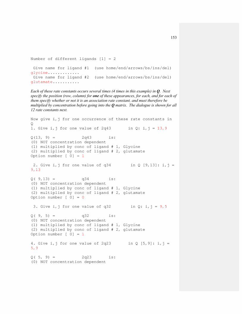
153

Number of different ligands [1] = 2 Give name for ligand #1 (use home/end/arrows/bs/ins/del) glycine............. Give name for ligand #2 (use home/end/arrows/bs/ins/del) glutamate........... Each of these rate constants occurs several times (4 times in this example) in Q. Next specify the position (row, column) for one of these appearances, for each, and for each of them specify whether or not it is an association rate constant, and must therefore be multiplied by concentration before going into the Q matrix. The dialogue is shown for all 12 rate constants next. Now give i,j for one occurrence of these rate constants in Q 1. Give i,j for one value of 2q43 in Q: i,j = 13,9 Q(13, 9) = 2q43 is: (0) NOT concentration dependent (1) multiplied by conc of ligand # 1, Glycine (2) multiplied by conc of ligand # 2, glutamate Option number [ 0] = 1 2. Give i,j for one value of q34 in Q [9,13]: i,j = 9,13 Q( 9,13) = q34 is: (0) NOT concentration dependent (1) multiplied by conc of ligand # 1, Glycine (2) multiplied by conc of ligand # 2, glutamate Option number [ 0] = 0 3. Give i,j for one value of q32 in Q: i,j = 9,5 Q( 9, 5) = q32 is: (0) NOT concentration dependent (1) multiplied by conc of ligand # 1, Glycine (2) multiplied by conc of ligand # 2, glutamate Option number [ 0] = 1 4. Give i,j for one value of 2q23 in Q [5,9]: i,j = 5,9 Q( 5, 9) = 2q23 is: (0) NOT concentration dependent

154

(1) multiplied by conc of ligand # 1, Glycine (2) multiplied by conc of ligand # 2, glutamate Option number [ 0] = 0 5. Give i,j for one value of beta1 in Q: i,j = 5,1 Q( 5, 1) = beta1 is: (0) NOT concentration dependent (1) multiplied by conc of ligand # 1, Glycine (2) multiplied by conc of ligand # 2, glutamate Option number [ 0] = 0 6. Give i,j for one value of alpha1 in Q [1,5]: i,j = 1,5 Q( 1, 5) = alpha1 is: (0) NOT concentration dependent (1) multiplied by conc of ligand # 1, Glycine (2) multiplied by conc of ligand # 2, glutamate Option number [ 0] = 0 7. Give i,j for one value of 2k43 in Q: i,j = 4,3 Q( 4, 3) = 2k43 is: (0) NOT concentration dependent (1) multiplied by conc of ligand # 1, Glycine (2) multiplied by conc of ligand # 2, glutamate Option number [ 0] = 2 8. Give i,j for one value of k34 in Q [3,4]: i,j = 3,4 Q( 3, 4) = k34 is: (0) NOT concentration dependent (1) multiplied by conc of ligand # 1, Glycine (2) multiplied by conc of ligand # 2, glutamate Option number [ 0] = 0 9. Give i,j for one value of k32 in Q: i,j = 3,2 Q( 3, 2) = k32 is: (0) NOT concentration dependent (1) multiplied by conc of ligand # 1, Glycine (2) multiplied by conc of ligand # 2, glutamate Option number [ 0] = 2

155

10. Give i,j for one value of 2k23 in Q [2,3]: i,j = 2,3 Q( 2, 3) = 2k23 is: (0) NOT concentration dependent (1) multiplied by conc of ligand # 1, Glycine (2) multiplied by conc of ligand # 2, glutamate Option number [ 0] = 0 11. Give i,j for one value of beta2 in Q: i,j = 2,1 Q( 2, 1) = beta2 is: (0) NOT concentration dependent (1) multiplied by conc of ligand # 1, Glycine (2) multiplied by conc of ligand # 2, glutamate Option number [ 0] = 0 12. Give i,j for one value of alpha2 in Q [1,3]: i,j = 1,2 Q( 1, 2) = alpha2 is: (0) NOT concentration dependent (1) multiplied by conc of ligand # 1, Glycine (2) multiplied by conc of ligand # 2, glutamate Option number [ 0] = 0 Now specify cycles that require a microscopic reversibility constraint to be applied (see above) Are there any cycles WITHIN independent units [N] ? N Next a blue box appears in which numerical values for the rate constants can ebe entered. The names of the parameters can be edited too (but not the specification of which ligand is bound in the third column)

12 rate constants name value ligand 1: 2q43 2.e8 glycine 2: q34 100 3: q3 1.e8 glycine 4: 2q23 200 5: beta1 2000 6: alpha1 1000 7: 2k43 2.e8 glutamate 8: k34 100 9: k32 1.e8 glutamate 10: 2k23 200 11: beta2 3000 12: alpha2 500

156

Now comes the tedious bit. Each of the rate constants appears four times, but the position of only one of these occurrences has been specified so far. The positions of all the others must be specified now. The other 3 occurrences of each is then set automatically (much like the constraints in HJCFIT, though the values entered below are kept, as part of the mechanism, separately from constraints applied while fitting). An attempt has been made to provide suitable defaults but may not always work 36 q(i,j) to be set same as the basic 12 rate constants Number of q(i,j) equal to q(13, 9) (rate( 1),2q43 ) [ 3] =3 1: specify i,j [ 0, 0] = 14,10 2: specify i,j [15,11] = 15,11 3: specify i,j [16,12] = 16,12 Number of q(i,j) equal to q( 9,13) (rate( 2),q34 ) [ 3] = 3 1: specify i,j [ 0, 0] = 10,14 2: specify i,j [11,15] = 11,15 3: specify i,j [12,16] = 12,16 And so on (for 10 more rate constants in this example) After this conductance of open states, voltage dependence of rate constants etc, are specified exactly as before, and the new mechanism (and rates) can be kept (in QMECHS.DAT)

157

SCALCS

This program calculates and displays various macroscopic properties of ion channels as described in Colquhoun & Hawkes (1977). Noise spectra, the response to various sorts of concentration jump, can be displayed and plotted. After defining the mechanism and rates as above, the main menu of options is as follows. (1) Calculate a c-jump (assuming initial equilibrium) (or specify arbitrary initial vector) (2) Calculate a c-jump (not assuming initial equilibrium) (3) Calculate relaxation in response to a conc-pulse (4) Calculate relaxation for conc-pulse with pre-pulse (5) Calculate relaxation with time-dependent concentration (6) Calculate noise spectrum (at -80.0 mV; 1.00000 muM) (7) As (1) but plot d/r curves for series of post jump conc (8) As (1) but plot binding curves for series of post jump

conc (9) As (1) but for range of values of a rate constant (10) Calculate response for a series of pulses Option number [ 1] = Option 1 is for a step change in concentration following a preincubation with a specified concentration (which may be zero) for long enough for equilibrium to be reached. Option two is similar, but the length of the preincubation is specified so the condition at the time of the step can be calculated. Options 3 and 4 calculate the responses to a rectangular agonist pulses (of specified concentration and duration), whereas option 5 can deal with some cases where the agonist concentration varies with time. Option 7 plots peak and steady state response against concentration, rather than against time, and 8, 9 do the same thing for binding and for values of the observed (macroscopic) rate constant(s). Once the type of jump is specified, the various concentrations are given. For example, with option 1, you may specify a step for 0 μM to 1.0 μM. The equilibrium occupancies of the 5 states at 1.0 μM are then printed out as follows. Subset Open Equilibrium Mean life Mean latency (ms) state occupancy (ms) to next shutting (#i) given start in i A 0.351805E-02 0.679515 1 0.293054E-04 0.990099E-01 0.106078 2 0.348874E-02 0.713857 0.713921 Subset Shut Equilibrium Mean life Mean latency (ms) state occupancy (ms) to next opening

158

(#i) given start in i B 0.196346E-01 0.979055E-01 3 0.976847E-04 0.142857E-01 168.614 4 0.195369E-01 0.988631E-01 590.099 C 0.976847 5.00000 5 0.976847 5.00000 595.099 This table also gives the equilibrium fraction in each subset (A, B, C –see SCBST), the mean duration of a sojourn in each state, and in each subset of states, and the mean latency to the next opening or shutting, conditional on the starting state. These numbers are often useful for spotting the physical significance of the macroscopic time constants.

The initial and final occupancies are then printed followed by the time constants and amplitudes of the exponential components that describe the time course of the current and of the binding. Then various things can be plotted (see help notes for plots). If you choose to plot the relaxation, you get the following options.

(1) Plot current (with exponential components) (2) Plot current only (3) Plot binding only (4) Plot current + binding (5) Plot occupancy of specified state(s) against time (6) Plot occupancy of a specified state with components (7) Plot specified transition frequencies vs time (8) Finish Option number [ 2] = For example, option 5 will show the time course of change of the occupancies of any (by default, all) of the individual states in the mechanism. Such plots can be very useful in understanding what underlies the macroscopic current (plotted in options 2 or 1). After the display, the curve may be fitted ‘experimentally’ with exponentials, in an attempt to see what might be fitted during analysis of an experiment in which not all components were separable. The curve can also be calculated over a new time rang (e.g. to expand the first few points, without loss of resolution). After the ‘concentration-response curve’ and ‘concentration-binding curve’ options (main menu, options 7 and 8) the following plotting options appear. Hill slope at equilibrium EC50 (2.404 muM) = 1.89215 (1) Plot peak and equilibrium concentration-response curves (2) Plot Hill-slope of (1) against concentration (3) Plot predominant rate constant against concentration (4) Plot slope of (2) against concentration (5) Finish Option number [ 1] =

159

There is now an option (2) to plot the Hill slope of the equilibrium curve against concentration, and the Hill slope at the EC50 is printed as above (the Hill slope is found numerically from adjacent points of the 512 points that make up the plotted curve). Option (3) allows the predominant rate constant (or time constant if this is chosen at the start) to be plotted against concentration. Finally there is an option to show the predicted time course for aligned bursts of activity in a steady state record (see Wyllie et al., 1998).

SCBST This calculates the properties of bursts of openings in the steady state, from the results given by Colquhoun & Hawkes (1982) [On the stochastic properties of bursts of single ion channel openings and of clusters of bursts, Phil. Trans. R. Soc. Lond. B300, 1-59]. After definition of the mechanism (as above), the concentration of agonist is approved. The definition of bursts that is used here depends on division of all the individual states in the mechanism into three subsets. Subset A contains all open states, whereas subset C contains long-lived shut states, such that one (or more) entries in to a C state will produce a shut time so long that the burst will be ended. Subset B contains short lived shut states in which shut times within a burst of openings are spent. For example, in the mechanism discussed above, at sufficiently low agonist concentration, only state 5, the resting unoccupied state would be in set C, the other three shut states being in set B. This would be specified as follows. number of open states, kA= 2 number of short shut states, kB=2 number of long-lived shut states C, kC=1 number of very long (between cluster) shut states, kD= 0

(NB kD=0 for this program) O.K. [Y] ? Remember that the numbering of the states must be such that the open states have the lowest numbers, and the C states have the highest numbers. The final line refers to a definition needed only when analysing clusters of bursts (as in Colquhoun & Hawkes, 1982), and that is not done in this program. Two things must be emphasised about the definition of bursts that is used here. (1) It is up to the user to check that, under the conditions used, the C states are indeed sufficiently long-lived to separate bursts clearly. The program does not check this. (2) Since it is impossible to tell which individual shut state the channel is in, it is not possible to define bursts of openings from an experimental record using this definition. For experimental analysis, bursts have to be defined by specifying a critical shut time (see EKDIST). If the shut times between bursts are much greater than shut times within

160

bursts, so the bursts are well separated, there will not be much difference between the theoretical definition of a burst and the experimental definition. Of course it would be possible (though more complicated) to make predictions of burst length etc that were based on the experimental definition of bursts, but such predictions would not have any simple physical interpretation. The reason for using the theoretical definition is that it allows a connection to be made between bursts that are observed in an experimental record, and the actual physical states of the channel. The default (short version) prints out the following distributions (in SCBST.PRT). (1) Distribution of the number of openings per burst (2) Distribution of the duration of the first opening in all bursts that have two or more

openings (3) Distribution of the duration of all open times (4) Distribution of the duration of the shut times within a burst (5) Distribution of the duration of the total open time per burst (6) Distribution of the duration of the burst length (7) Distribution of the duration of the shut times between bursts (8) Distribution of the duration of all shut times

These are all calculated from the equations given by Colquhoun & Hawkes (1982).

At the end there are calculations that allow comparison of the theoretical definition of bursts that were used for the calculations, and the experimental definition based on a critical shut time.

The long version of the program, which can be chosen at the start, will also print out distributions that are conditional on the initial state. For example, it will calculate the distribution of number of openings for bursts that start in open state 1, and for those that start in open state 2, as well as the overall distribution. (These conditional distributions cannot be observed experimentally unless the two open states have different conductances, but they may be a useful aid for understanding the physical basis of the observations.) It will also calculate distributions of things like the length of the 3rd opening in all bursts that have 5 openings etc.

SCCOR This program calculates the correlations between open-open, open shut and shut-

shut times, as a function of lag. It also calculates the correlation between durations of the first and the kth opening within a burst (bursts being defined by the subsets of states described in the SCBST notes).

After the mechanism and values for the rate constants, have been defined, as above, simply define the number of lags required (for example open-open correlation with lag=2 means the correlation between the length of an opening and the length of the next but one opening). The calculations are done according to the results given by Colquhoun & Hawkes (1987) [A note on correlations in single ion channel records. Proc. R. Soc. Lond. B 230,15-52.]. At the end of the program you can also calculate the distribution of open times conditional on the openings being adjacent to shut times in a

161

specified range (the perfect resolution version of the conditional distribution use in HJCFIT). This is calculated as described in Colquhoun, Hawkes. & Srodzinski, (1996). [Joint distributions of apparent open times and shut times of single ion channels and the maximum likelihood fitting of mechanisms. Philosophical Transactions of the Royal Society London A 354, 2555-2590.]

SCJUMP

This program calculates various properties of single channels following a jump, or pulse, in agonist concentration (voltage jumps not yet fixed). The calculations are done as described by Colquhoun & Hawkes (1997) [Properties of single ion channel currents elicited by a pulse of agonist concentration or voltage. Philosophical Transactions of the Royal Society London A. 355, 1743-1786]. After the mechanism and values for the rate constants, have been defined, as above, state what sort of concentration jump or pulse is required. For example, a 1 ms pulse of 1 mM agonist, starting from and reverting to zero concentration, would be described as follows on the screen. (1) Calculate a c-jump (assuming initial equilibrium) (2) Calculate a c-jump (not assuming initial equilibrium) Option number [2] = 2 Initial and final concentrations = 1000.00 0.000000 muM: O.K. [Y] ? Y Length of exposure to 1000.00 muM (ms) [1.00] = 1 Concentration before this (muM) [0.00] = 0 (notice that this describes channels after the step to zero concentration, not during the pulse).

Many sorts of distribution are then printed out, as described by Colquhoun & Hawkes (1997). The particular case of a concentration jump to zero concentration can give rise to problems because various matrices become singular at zero concentration. This is a common case, because it is the sort of calculation that will often be done to mimic a pulse of transmitter at a synapse, so the program is written to cope with these problems. In order to do such calculations it may be necessary to redefine the subset, C, of long-lived shut-states so that it is absorbing (cannot be left) at zero concentration, as described by Colquhoun & Hawkes (1997), and the program will do this.

SCSIM

This program generates simulated experimental data. The output consists of a list of open times, shut times and amplitudes, as would be produced form experimental

162

results in SCAN (a SCAN.SCN file). It is possible to simulate either a steady state experiment or a jump or jump experiment, and in the former case the program can also generate a simulated CONSAM file, with added white noise, that can be analysed in SCAN as though it were a real experiment. The SCAN.SCN file can be analysed in EKDIST or HJCFIT as though it were from an experiment. Most simulation programs work by generating the state of the system at fixed time points, so it is necessary to define how far apart these time points should be, a question about which there is always some ambiguity. In SCSIM, advantage is taken of two facts. (a) The distribution of the length of time spent in any individual state is exponentially distributed (with mean –qii for state i) and (b) a random exponentially distributed value with mean τ can be generated as z= − τ log(u), where u is a random (uniformly-distributed) value between 0 and 1. This method can be extended to time-varying concentrations as described below.

Values of u are generated by the high quality pseudo-random number generator described by Wichmann & Hill.( 1985,. An efficient and portable pseudo-random number generator. In Applied Statistics Algorithms, ed. Griffiths, P., pp. 238-242. Ellis Horwood, Chichester). This requires three integer seed values. The current values of these are kept on disk (in the file RANDOM.DAT) so you can choose to repeat an identical random number sequence if you need to, though normally the values at the end of one run are used as seeds for the next run (if a sample were taken continuously every ms it would take 220 years for the sequence to repeat).

First the mechanism and rates are defined, exactly as in the other theory programs. Then say if a new random number sequence is to be used, how many intervals are to be generated and so on. Note that many individual sojourns in interconnected shut states may be needed to generate a single ‘observed’ shut time (and similarly for open states of equal conductance).

Derivations for channel simulations with time-varying concentration

D. Colquhoun and A.G. Hawkes (original notes, 15-Feb-91) When concentration varies with time, we can no longer ignore the time at which a sojourn starts (for any state the lifetime of which is concentration-dependent). Therefore the usual equation must be re-written to specify the time, t0 say, at which the sojourn starts (we suppose that the concentration at this time is known). Thus, rather than considering the interval t, t +Δt (or just 0, Δt) we must formulate the problem as follows. For any particular state Prob[leave state in interval t0+t, t0+t +Δt⏐in that state at t0] = αc(t0+t)Δt + βΔt + o(Δt) (1) where α = sum of concentration-dependent rate constants for leaving, and β = sum of rate constants that are independent of concentration.

163

Now define P(t;t0) = Prob[ in specified state throughout interval t0 to t0+t⏐in that state at t0] (2) Thus P(t+Δt ; t0) = P(t ; t0).Prob[does not leave in Δt]

=P(t ; t0).[1 - αc(t0+t) Δt - βΔt - o(Δt)] (3)

so

⎟⎠⎞

⎜⎝⎛

ΔΔ

+++−=Δ

−Δ+

ttttcttPt

ttPtttP )o()();()0;();(

00

0βα (4)

and letting Δt →0 we get

])([);(d

)0;(d00 βα ++−= ttcttP

t

ttP (5)

so, if channel the lifetime is z

d dP t tP t tt

z zP z t c t t t( ; )

( ; ) log ( ; ) [ ( ) ]000 0 00=∫ ∫= = − + +α β (6)

⎥⎦⎤

⎢⎣⎡ +−=⎥⎦

⎤⎢⎣⎡ ++−= ∫∫

+

=

zt

t

z

tzttcztttca 0

0

d).(d)(0 0 βαβ (7)

so

⎥⎦⎤

⎢⎣⎡ ⎟

⎠⎞⎜

⎝⎛ +−= ∫

+zt

tzttctzP 0

0

]d)(exp);( 0 βα (8)

= Prob[ life time > z ⏐ life started at t0] = 1 − F(z) (9)

164

Simulation with random number generator (method suggested by A.G. Hawkes) To simulate want 1 − F(z) = u, where u has uniform (0, 1) distribution. (1) If concentration is constant then 1 − F(z) = exp(−z/τ) where τ = 1/(αc+β) = mean channel lifetime, so the simulated lifetime is z= − τ log(u), as usual. (2) Exponentially rising and falling concentration. Say c t c t t( ) [exp( / ) exp( / )]= − − −m d rτ τ (10) where τd, τr are the time constants for decay and rise of concentration. In this case we need

∫+

+=−=−zt

t

zttcutzP0

0

d)()log());(log( 0 βα

zztztc βττττττα +−−−−−−−= ))]/exp(1)(/exp())/exp(1)(/exp([ rr0rdd0dm (11) For given u this can be solved numerically for z (note u = 1 gives z = 0). However before trying to do so, we must first see if lifetime is infinite. Infinite lifetimes when β = 0.

For z → ∞ in (11) we get, when β = 0, ))/exp()/exp(()log( r0rd0dmmin ττττα ttcu −−−=− or ),(]}/exp()/exp([exp{ 0r0rd0dmmin tPttcu ∞=−−−−= ττττα (12) so umin is the probability that a lifetime is infinite, i.e. the concentration has decayed to essentially to zero without any occupancy ever occurring. Hence any value of u < umin gives an infinite lifetime; above umin the lifetime decreases, very rapidly at first, until it approaches 0 as u approaches 1. To apply Newton-Raphson to (11) we need its first derivative with respect to z, viz

βττττα +−−−−− )]/exp()/exp()/exp()/[exp( rr0dd0m ztztc (13) Some trouble was encountered with the pure Newton-Raphson method, but a routine based on RTSAFE (from Numerical Recipes) works beautifully; this method constrains z by using a bisection step if the solution goes out of bounds, before reverting to Newton.

165

In this case, z was constrained to be positive by setting bounds 0 to 1010 with an initial guess of z = 1 ms. (3) Case of a rectangular concentration pulse. This is useful, if only because the result can be checked against the eigenvalue solution. Say the concentration is constant from t = 0 to t = td, and then falls to zero.

c t c t tc t t t( ) ,( ) ,

= < <= >

m d

d

00

(14) For any state for which all the exit routes involve binding (β = 0), its lifetime is infinite if the sojourn starts after td; if the sojourn starts before td then define the time left from when the sojourn starts to when the concentration falls as t t t1 = −d 0 (15) If the sojourn ends after the end of the pulse, the time from the end of the pulse to the end of the sojourn is defined as t t z t z t2 1= + − = −0 d , so z t t= +1 2 t=0 t0 td t0+z t1 t2

The general result is

− = ++

∫log( ) ( )u c t t zt

t z

α βd0

0

= (αcm + β)z if t0 + z < td , (16) so when t0 + z < td (i.e. the sojourn ends before the concentration falls so cm is constant throughout) we have, as usual,

zu

cu=

−+

= −log( )

log( )α β

τm

(17)

conc

vacant occupied z

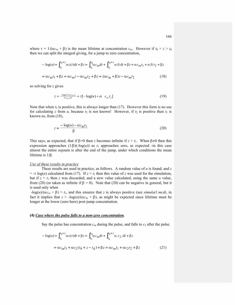
166

where τ = 1/(αcm + β) is the mean lifetime at concentration cm. However if t0 + z > td then we can split the integral giving, for a jump to zero concentration, − = + = + + = + +

+ +∫ ∫∫log( ) ( ) . . . .u c t t z c t t z c t t ztt z

tt z

tt

α β α α β α α βd d dm md

d

0

0 0

00 01 2

= + = − + = + −α β α α β α β αc t z c z c t z c z c tm m m m m1 2 2( ) (18) so solving for z gives ])log([ 2m

)log(m

2m tcuz ctcu ατβα

α +−== ++− (19)

Note that when t2 is positive, this is always longer than (17). However this form is no use for calculating z from u, because t2 is not known! However, if t2 is positive then t1 is known so, from (18),

zu c t

=− −log( ) α

βm 1 (20)

This says, as expected, that if β=0 then z becomes infinite if z > t1. When β≠0 then this expression approaches (1/β)(-log(u)) as t1 approaches zero, as expected -in this case almost the entire sojourn is after the end of the jump, under which conditions the mean lifetime is 1/β. Use of these results in practice

These results are used in practice, as follows. A random value of u is found, and z = -τ log(u) calculated from (17). If z < t1 then this value of z was used for the simulation, but if z > t1 then z was discarded, and a new value calculated, using the same u value, from (20) (or taken as infinite if β = 0). Note that (20) can be negative in general, but it is used only when -log(u)/(αcm + β) > t1, and this ensures that z is always positive (see simulat1.mcd), in fact it implies that z > -log(u)/(αcm + β), as might be expected since lifetime must be longer at the lower (zero here) post-jump concentration. (4) Case where the pulse falls to a non-zero concentration. Say the pulse has concentration cm during the pulse, and falls to c2 after the pulse.

− = + = + ++ +

∫ ∫∫log( ) ( ) . .u c t t z c t c t ztt z

tt z

tt

α β α α βd d dmd

d

0

0 0

02

= + + − + = + +α α β α α βc t c t z t z c t c t zm 2 d m 21 0 1 2( ) (21)

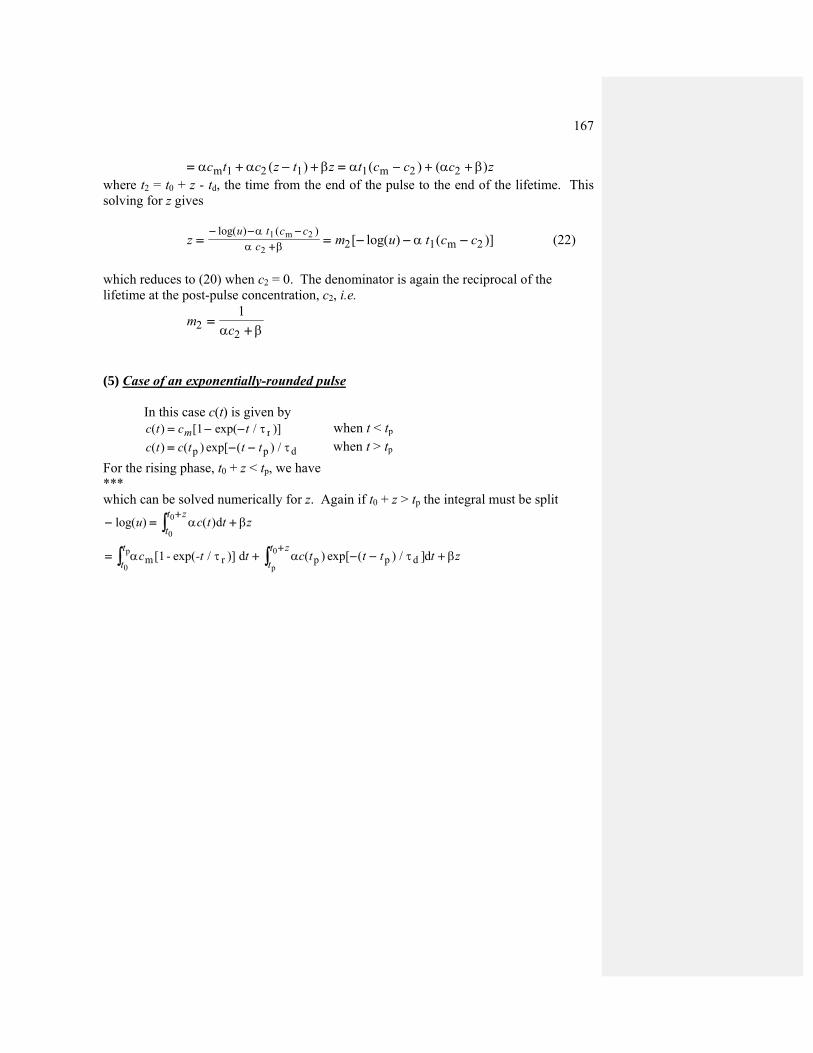
167

= + − + = − + +α α β α α βc t c z t z t c c c zm 2 m 21 1 1 2( ) ( ) ( ) where t2 = t0 + z - td, the time from the end of the pulse to the end of the lifetime. This solving for z gives

z m u t c cu t c c

c= = − − −− − −

+log( ) ( )

[ log( ) ( )]α

α β α1 22 1 2

m

2 m (22)

which reduces to (20) when c2 = 0. The denominator is again the reciprocal of the lifetime at the post-pulse concentration, c2, i.e.

mc2

2

1=

+α β

(5) Case of an exponentially-rounded pulse In this case c(t) is given by

c t c tm( ) [ exp( / )]= − −1 τ r when t < tp c t c t t t( ) ( ) exp[ ( ) /= − −p p dτ when t > tp

For the rising phase, t0 + z < tp, we have *** which can be solved numerically for z. Again if t0 + z > tp the integral must be split

− = +

= + − − +

+

+

∫

∫∫

log( ) ( )

( ) exp[ ( ) / ]

u c t t z

c -t t c t t t t z

tt z

tt z

tt

α β

α τ α τ β

d

[1 - exp( / )] d dm r p p dp

p

0

0

0

0