I

Manual for Code

VISCO-PLASTIC SELF-CONSISTENT (VPSC)

Version 7c

(last updated: November 13, 2009)

C.N. Tomé

(Los Alamos National Laboratory - USA) tome@lanl.gov

and

R.A. Lebensohn

(Los Alamos National Laboratory - USA) lebenso@lanl.gov

II

INDEX

Copyright / Disclosure ……………………………………………………. 1

General Description / Recommendation …………..……..………………. 2

What’s new in VPSC7………………………………..…………..……..… 3

SECTION 1: Theory and Models

1-1 Introduction ………………………..……………………………. 4

1-2 Kinematics …………………………….………………………… 4

1-3 Updating crystal orientation and grain shape …………………… 6

1-3-1 Crystallographic & morphologic texture rotation

1-3-2 Grain co-rotation

1-5 Self-consistent polycrystal formalism……………………………. 8

1-5-1 Local behavior and homogenization

1-5-2 Green function and Fourier transform

1-5-3 Viscoplastic inclusion and Eshelby tensors

1-5-4 Interaction and localization equations

1-5-5 Self-consistent equations

1-5-6 Algorithm

1-5-7 Secant, affine, tangent and intermediate linearizations

1-6 Hardening of slip and twinning systems………………………… 21

1-6-1 Voce hardening

1-6-2 MTS hardening

1-7 Twinning model ………………………………………………… 26

1-8- Second order formulation ……………………………………..… 27

1-8-1 Second order moments

1-8-2 Second order procedure

1-8-3 Numerical implementation

1-9 References……………………………………………………….. 33

III

SECTION 2: Description of VPSC code

2-1 Numerical algorithm……………………………………………… 35

2-2 Simulation of deformation: Input/Output options………………… 36

2-3-1 Grain shape evolution option

2-3-2 Variable velocity gradient option

2-4 Code architecture ………………………………………………. 41

2-5 Units, reference system and conventions ..…………………….. 42

2-6 Description of Input files……………………………………….. 44

2-7 Description of Output files……………………………………… 55

2-8 Interfacing VPSC with FE codes (VPSC7FE) ….……………… 62

SECTION 3: Examples and applications of VPSC code

Example 1: Tension and Compression of FCC ………………..…… 66

Example 2: Rolling of FCC ………………………………………… 70

Example 3: Rolling of BCC ………………………………………… 74

Example 4: Rolling of a 2-phase FCC+BCC aggregate ……….…… 77

Example 5: Torsion of FCC …..…………………………………….. 79

Example 6: Application of MTS model to rolled aluminum ……….. 82

Example 7: Twinning and anisotropy of HCP zirconium …………… 85

Example 8: Compression of (orthorhombic) olivine ………………… 91

Example 9: Compression of ice (constant rate and creep)…………… 94

Example 10: Equal Channel Angular Extrusion of FCC…………… 98

Examples of VPSC7FE ……………………………………………… 100

SECTION 4: Appendices

Appendix A: Taylor factor ………………..……………………… 102

Appendix B: Von Mises equivalent stress & strain ………………..… 105

Appendix C: Voce hardening and algorithm ………………..…… 107

Appendix D: Crystal rotation and misorientation ………………..…… 109

1

Code Visco-Plastic Self-Consistent (VPSC)

Version 7c – November 2009

C.N. Tomé, Los Alamos National Laboratory, USA, tome@lanl.gov

R.A. Lebensohn, Los Alamos National Laboratory, USA, lebenso@lanl.gov

==============================================================

COPYRIGHT NOTICE

Portions of this program were prepared by the Regents of the University of California at

Los Alamos National Laboratory (the University) under Contract No. W-7405-ENG-36

with the U.S. Department of Energy (DOE). This software can be identified by the code

LA-CC-99-72 issued by the Classification Office of Los Alamos National Laboratory.

The University has certain rights in the program pursuant to the contract and the program

should not be copied or distributed outside your organization. All rights in the program

are reserved by the DOE and the University. Neither the U.S. Government nor the

University makes any warranty, express or implied, or assumes any liability or

responsibility for the use of this software.

==============================================================

DISCLOSURE

We distribute this code free of charge on a personal basis and ask you not to make it

available to other users. We would appreciate if you acknowledge its use when reporting

your results.

These notes contain a description of the theory, the capabilities of the VPSC code, and

several examples. The code itself is in a permanent state of change and new options, bug-

fixes and changes are incorporated as required by new developments, new applications,

or as suggested by interactions with the users. In addition, not every possible combination

of running conditions is tested when the code is modified. As a consequence use it at

your own risk and let us know if you find bugs or run into trouble while using it. We

2

appreciate comments and suggestions that may improve the interface with the users. We

strongly recommend running the benchmark cases included in the examples and make

sure that you can reproduce the same results.

GENERAL DESCRIPTION

VPSC is a computer code written in FORTRAN 77 which simulates the plastic

deformation of polycrystalline aggregates. VPSC stands for Visco Plastic Self Consistent

and refers to the particular mechanical regime addressed (VP) and to the approach used

(SC). VPSC was developed for application to low-symmetry materials (hexagonal,

trigonal, orthorhombic, trigonal), although it also performs well on cubic materials.

VPSC accounts for full anisotropy in properties and response of the single crystals and

the aggregate. It simulates the plastic deformation of aggregates subjected to external

strains and stresses. VPSC is based on the physical shear mechanisms of slip and

twinning, and accounts for grain interaction effects. In addition to providing the

macroscopic stress-strain response, it accounts for hardening, reorientation and shape

change of individual grains. As a consequence, it predicts the evolution of hardening and

texture associated with plastic forming. The simulation procedure can be applied to

deformation of metals, intermetallics and geologic aggregates.

RECOMMENDATION

The VPSC7 manual includes a thorough description of the related theory. Most of

Section 1 can be skipped if you are only interested in running the code. However,

Subsections 1-6 and 1-7, dealing with hardening and twinning models, should be read. In

addition, most of Section 2, describing input and output files, should be read. The user is

advised to become familiar with the examples in Section 3, because they highlight

different capabilities of the code. Reproducing the numerical results of the examples is

highly recommended both, to become familiar with the input/output files and procedures,

and to make sure that the code was properly installed in the user’s computer.

When compiling VPSC, always use the double precision option.

3

WHAT IS NEW IN VPSC7 ?

By comparison with VPSC6, several features and improvements were added to VPSC7.

In general: we have improved and accelerated some of the numerical algorithms,

subroutines have been added/modified aiming for more flexibility and modulation in the

code, and the structure of the main input file (VPSC7.IN) has changed a bit.

The new capabilities of the code are:

* We have retained (from VPSC6) the full constraints, secant, tangent and neff

=10

linearization procedures that control grain-matrix interaction.

* We have implemented a new ‘affine’ linearization procedure which allows the user to

run simulations where different deformation modes may have different rate sensitivities

(parameter NRS). This more rigorous feature replaces the rather empirical approach to

this problem implemented in VPSC6.

* We have implemented a new ‘second order’ linearization procedure based on

calculating and using intragranular stress fluctuations for describing the grain response.

This procedure is onerous in computing time but is more appropriate for simulation of

systems with large variations in stiffness between grains (either directional variations

because of anisotropy, or grain-to-grain variations associated with multi-phase systems).

* We have retained (from VPSC6) the capability to impose mixed stress and strain-rate

boundary conditions, and we have added the possibility of enforcing a stress component

as test control. This feature allows for simulations of creep tests.

* A new type of ‘process’ was added. When ivgvar=4 the code rotates rigidly the

crystallographic and morphologic texture of the aggregate without imposing deformation.

4

SECTION 1: THEORY AND MODELS

1-1 INTRODUCTION

During plastic forming the contribution to deformation from elasticity is negligibly small

(typically 10-3

) by comparison to the plastic component (typically >10-1

). In addition,

once the elasto-plastic transition is over, the evolution of stress in the grains is controlled

by plastic relaxation (slip activity). This means that the size and evolution of the single

crystal yield surface controls the stress in the grain. As a consequence, in our formulation

we disregard elasticity and describe only plastic contribution to deformation.

1-2 KINEMATICS

In this Section we provide a brief overview of the equations used in kinematics. They

apply to any continuum plastic body and, in particular, to crystallographic grains and to

aggregates. The reader is referred to the book of Gurtin (1981) for a comprehensive

treatise on kinematics. We define:

X : initial coordinates of a point in the undeformed crystal

x(X) : final coordinates of a point in the deformed crystal

u=x-X : displacement of the point

The deformation in the grain is characterized by the displacement gradient tensor Lc and

the deformation gradient tensor Fc , defined as:

j

cic

ij x

uL

∂

∂=ɺ

(2-1)

j

icij X

xF

∂

∂= (2-2)

With the property:

i ij jx F X= (2-3)

Using the definitions of the different tensors it can be shown that:

ccc F:LF =ɺ (2-4)

5

In addition, since plastic deformation is accommodated by shear, and since shear

preserves the orientation of the crystal, it is useful to utilize what is called the ‘polar

decomposition’ of the deformation gradient. Such procedure amounts to treat

displacements as two sequential steps: a ‘plastic stretch’ coF which distorts the crystal

without reorienting it, followed by a rigid crystal rotation cR that transforms from initial

to final crystal axes:

c

o

cc F.RF = (2-5)

In crystal axes the stretch obeys a relation like (2-4):

co

co

co FLF =ɺ (2-6)

where

j

cic

o X

uL

ij ∂

∂=ɺ

(2-7)

is the velocity gradient in the reference frame attached to the crystal axes, given by the

linear superposition of shear rates on all active slip and twinning systems:

sj

si

s

sco

nbLij

∑ γ= ɺ (2-8)

The vectors n and b remain invariant in crystal axes. Decomposing the dyadic ss nb ⊗

into the symmetric and skew symmetric components:

( )( )s

isj

sj

si2

1sij

si

sj

sj

si2

1sij

nbnbq

nbnbm

−=

+= (2-9)

allows us to decompose the velocity gradient into a strain rate and a rotation rate (spin):

co

co

co ijijij

WDL += (2-10a)

where

∑ γ=s

sij

sco

mDij

ɺ (2-10b)

∑ γ=s

sij

sco

qWij

ɺ (2-10c)

6

Replacing (2-5) in (2-3) and using (2-6):

( ) Tcc0

cTccTc1c0

c0

cc0

c1cc0

c RLRRRRFFRFRFFL +=

+==

−−ɺɺɺɺ (2-11)

Which can be decomposed, using (2-10), into a strain rate and a rotation rate:

cij

cij

cij

WDL += (2-12)

where

+=+=

==TccR,c

o

TccTcco

cc

R,co

Tcco

cc

RRWRRRWRW

DRDRD

ɺɺ

(2-13)

The distortion rate Dc is simply a transformation from crystal into ‘current’ frame, but the

rotation rate Wc contains an extra contribution.

1-3 UPDATING CRYSTAL ORIENTATION AND GRAIN SHAPE

The kinematics expressions of the previous section are completely general, and

applicable to any polycrystal model. Specifically, the polycrystal model will provide a

value for the velocity gradient in each grain ccc WDL += . With it we do the following:

1) We use (2-13) to obtain the rate of change of the crystal orientation matrix

cR,co

cc R)WW(R −=ɺ (3-1)

which is in turn used to update incrementally the orientation of the crystal and, as a

consequence, to follow the texture evolution. The matrix cRɺ is skew-symmetric and, as

a consequence, cR t∆ɺ does not represent a transformation and cannot be used to calculate

an incremental rotation of the crystal. Instead, the Rodrigues formula has to be used. See

Appendix D for explanation and SUBROUTINE RODRIGUES for algorithm. The

calculation ofcRɺ is done in SUBROUTINE UPDATE_ORIENTATION.

2) We use an incremental form of (2-4) for updating the deformation gradient of the

grain:

oldcccoldcnewc F)tLI()tFF(F ∆+=∆+= ɺ (3-2)

7

(See SUBROUTINE UPDATE_FIJ).

3) We use the updated deformation gradient to update the shape of the grain as follows:

assume a spherical locus of points X in the undeformed state, which obey the equation

1XX T =⋅ (3-3)

The corresponding locus in the deformed state can be calculated using Eq (2-4) as:

1xx)FF( kj1

jkT =⋅ − (3-4)

which is the equation of a general ellipsoid. The eigenvectors and the (square root of the)

eigenvalues of )FF( T⋅ define the direction and length of the axes of the ellipsoid which

represents the grain.

(See SUBROUTINE UPDATE_SHAPE).

1-3-1 CRYSTALLOGRAPHIC & MORPHOLOGIC TEXTURE ROTATION

Section 1-3 above gives the kinematic expressions used to update crystal axes orientation

and the grain’s deformation gradient. These magnitudes are updated incrementally by

VPSC during a deformation simulation. However, there are some situations when the

ellipsoid and the ‘attached’ crystal axes need to be rotated rigidly with respect to a

‘laboratory’ reference system. VPSC allows the user to apply a ‘process’ (IVGVAR=4)

which is a rigid rotation of the crystallographic and morphologic textures. This is done

inside SUBROUTINE TEXTURE_ROTATION. The input in this case is the rotation

matrix ROTMAT that operates on crystallograpic and morphologic texture as follows:

a- rigid rotation of the sample with respect to laboratory axes: ROTMAT rotates the

sample from 'old' to 'new position. Columns of ROTMAT are the sample axes after

rotation, expressed in the laboratory system. An example of this process is sequential

passes during ECAE route: the sample leaving the exit channel of the die is rotated and

reinserted into the entry channel. The texture and grain shape need to be referred to the

axes attached to the die (lab system)

b - change of reference system : columns of ROTMAT are 'old' system axes expressed

in 'new' system. ROTMAT transforms vectors and tensors expressed in 'old' set of axes,

and expresses their components in 'new' set of axes:

8

vnew(i) =rotmat(i,j)*vold(j) and tnew(i,j)=rotmat(i,k)*rotmat(j,l)*told(k,l)

An example is a Lankford test, where tension is applied at an angle α with respect to the

rolling direction. For numerical simplicity in applying load conditions it is easier to

assume that the tensile direction is always ‘axis 1’, and that the rolling texture appears as

rotated by α with respect to such system.

1-3-2 GRAIN CO-ROTATION

It is to be expect that the reorientation of a grain during deformation will be affected (to

some extent) by the neighboring grains. Specifically, if neighboring grains exhibit

different reorientation trends, it can be expected that they will ‘drag’ each other. An

empirically simple way of accounting for such effect inside VPSC is to assign a neighbor

at random to every grain, to calculate the spin of each grain ‘c’ (given by )WW( co

c − ),

to average the spin of the two randomly paired grains, and to assign this average spin to

each of them. As a result of this procedure grains with the same initial orientation will

reorient differently during deformation because each of them will interact with a different

neighbor (see Tomé, Lebensohn, Necker (2002) for details).

This procedure is controlled by the variable NNEIGH which is read from file VPCS6.IN.

If NNEIGH=0 no neighbor is assigned, and if NNEIGH=1 one neighbor is assigned to

each grain.

(see SUBROUTINE_NEIGHBOURS)

1-5 SELF-CONSISTENT POLYCRYSTAL FORMALISM

In what follows, we present the basic equations of the 1-site viscoplastic selfconsistent

model, originally due to Molinari et al (1987) and extended to fully anisotropic behavior

by Lebensohn and Tomé (1993). The present derivation is completely general, based on

the fully incompressible formulation of Lebensohn et al. (1998a) and the generalized

affine linearization scheme of Masson et al. (2000). Comprehensive derivations can be

found in Lebensohn et al. (2004) and Tomé and Lebensohn (2004).

9

In brief, the polycrystal is represented by means of weighted orientations. The

orientations represent grains and the weights represent volume fractions. The latter are

chosen to reproduce the initial texture of the material. Each grain is treated as an

ellipsoidal visco-plastic inclusion embedded in an effective visco-plastic medium. Both,

inclusion and medium have fully anisotropic properties. The effective medium represents

the ‘average’ environment ‘seen’ by each grain. Deformation is based on crystal

plasticity mechanisms -slip and twinning systems- activated by a Resolved Shear Stress.

1-5-1 Local constitutive behavior and homogenization

Let us consider a polycrystalline aggregate. The viscoplastic constitutive behavior at local

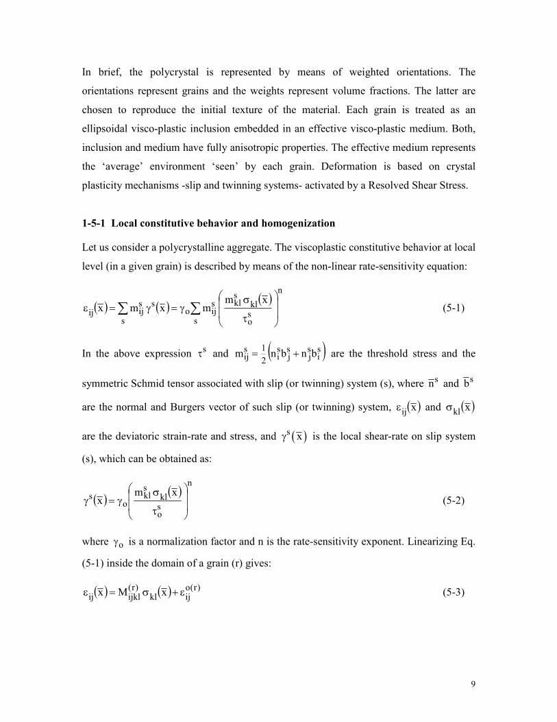
level (in a given grain) is described by means of the non-linear rate-sensitivity equation:

( ) ( )( )

n

sso

klskls

ijos

s

sijij

xmmxmx ∑∑

τ

σγ=γ=ε (5-1)

In the above expression sτ and ( )si

sj

sj

si2

1sij bnbnm += are the threshold stress and the

symmetric Schmid tensor associated with slip (or twinning) system (s), where sn and sb

are the normal and Burgers vector of such slip (or twinning) system, ( )xij

ε and ( )xkl

σ

are the deviatoric strain-rate and stress, and ( )s xγ is the local shear-rate on slip system

(s), which can be obtained as:

( )( )

n

so

klskl

os xm

x

τ

σγ=γ (5-2)

where oγ is a normalization factor and n is the rate-sensitivity exponent. Linearizing Eq.

(5-1) inside the domain of a grain (r) gives:

( ) ( ) )r(oijkl

)r(ijklij

xMx ε+σ=ε (5-3)

10

where )r(

ijklM and

)r(oij

ε are the viscoplastic compliance and the back-extrapolated term of

grain (r), respectively. Same relation holds for the average strain-rate and stress in grain

(r):

)r(oij

)r(kl

)r(ijkl

)r(ij

M ε+σ=ε (5-4)

Depending on the linearization assumption, )r(

ijklM and

)r(oij

ε can be chosen differently.

Later in this section we discuss the possible choices for the local linearized behavior.

Performing homogenization on this linearized heterogeneous medium consists in

assuming a linear relation analogous to (5-3) at the effective medium (polycrystal) level:

oijklijklij

EME +Σ= (5-5)

where ij

E and ijΣ are overall (macroscopic) magnitudes and ijklM and oijE are the

macroscopic viscoplastic compliance and back extrapolated term, respectively. The latter

moduli are unknown a priori and need to be adjusted self-consistently. Invoking the

concept of the equivalent inclusion (Mura 1987), the local constitutive behavior can be

rewritten in terms of the homogeneous macroscopic moduli, so that the inhomogeneity is

’hidden’ inside a fictitious eigen-strain-rate, as:

( ) ( ) ( )xExMx *ij

oijklijklij

ε++σ=ε (5-6)

( )x*ijε is the eigen-strain-rate field, which follows from replacing the inhomogeneity by

an equivalent inclusion. Rearranging and subtracting (5-5) from (5-6) gives:

( ) ( ) ( )( )xx~Lx~ *klklijklij ε−ε=σ (5-7)

The symbol "~" denotes local deviations of the corresponding tensor from macroscopic

values and 1ijklijkl ML −= . Combining (5-7) with the equilibrium condition:

( ) ( ) ( ) ( )x~x~x~x mi,j,ij

cj,ij

cj,ij σ+σ=σ=σ (5-8)

11

where cσ and mσ are the Cauchy and mean stresses, respectively. Using the relation

( ) ( ) ( )( )xu~xu~x~i,jj,i2

1ij +=ε between strain-rate and velocity-gradient, and adding the

incompressibity condition, we obtain:

( ) ( ) ( )( ) 0xu~

0xfx~xu~L

k,k

imi,lj,kijkl

=

=+σ+

(5 9a)

(5 9b)

−

−

where the fictitious volume force associated with the heterogeneity is:

( ) ( ) ( )xxLxf *j,ij

*j,klijkli σ=ε−= (5-10)

The field ( ) ( )xLx *klijkl

*ij ε−=σ defined in (5-10) will be called in what follows eigen-

stress field.

1-5-2 Green function method and Fourier transform solution

System (5-9) consists of four differential equations with four unknowns: three are the

components of velocity deviation vector ( )xu~i , and one is the mean stress deviation

( )x~mσ . A system of N linear differential equations with N unknown functions and an

inhomogeneity term, such as (5-9), can be solved using the Green function method, as

explained in what follows. Let us call ( ) ( )xHandxG mkm the Green functions

associated with ( )xu~i and ( )x~mσ , which solve the auxiliary problem of a unit volume

force, with a single non-vanishing m-component, and applied at 0x = :

( ) ( ) ( )( ) 0xG

0xxHxGL

k,km

imi,mlj,kmijkl

=

=δδ++

(5 11a)

(5 11b)

−

−

Here ( )xδ is Dirac’s delta function and δim is the Kronecker delta. Once the solution of

(5-11) is obtained, the solution of (5-9) is given by the convolution integrals:

( ) ( ) ( )∫ ′′′−=3R

ikik xdfGu~ xxxx (5-12)

12

( ) ( ) ( )∫ ′′′−=σ3R

iim xdxfxxHx~ (5-13)

System (5-11) can be solved using the Fourier transform method (Lebensohn et al.,

2003). Expressing the Green functions in terms of their inverse Fourier transforms, the

differential system (5-11) transforms into an algebraic system:

( ) ( )( ) 0kGk

kHikkGkL

km2

k

immikm2

ijkllj

=α

δ=α+αα

(5 14a)

(5 14b)

−

−

where k and α are the modulus and the unit vector associated with a point of Fourier

space α= kk , respectively. Calling ijkllj

dik

LA αα= , system (5-14) can be expressed as

a matrix product CBA =× where A, B and C are matrices given by:

C

000

100

010

001

0

AAA

AAA

AAA

A

B

HikHikHik

GkGkGk

GkGkGk

GkGkGk

321

3d33

d32

d31

2d23

d22

d21

1d13

d12

d11

321

332

322

312

232

222

212

132

122

112

=

ααα

α

α

α

=

=

(5-15)

The 4x4 matrix A is real and symmetric. As a consequence, its inverse will also be real

and symmetric. Using the explicit form of matrix C, we can write the solution of (5-15)

as:

=×=

−−−

−−−

−−−

−−−

−

143

142

141

133

132

131

123

122

121

113

112

111

1

AAA

AAA

AAA

AAA

CAB (5-16)

Finally, comparing (5-15) and (5-16):

1ijij

2 AGk −= (5-17)

13

1i4i AHik −= (5-18)

Since the components of A are real functions of αi , so are the components of A-1

, and so

are ij2Gk and iHik . This property leads to real integrals in the derivation that follows.

1-5-3 Viscoplastic inclusion and Eshelby tensors

Now that we have a solution for the Green tensors, we can write the solution of our

eigen-strain-rate problem using the convolution integrals (5-12)-(5-13). Taking partial

derivatives to Eq. (5-14) we obtain:

( ) ( ) ( )∫ ′′′−=3R

il,kil,k xdfGu~ xxxx (5-19)

Replacing (5-10) in (5-19), recalling that ( ) ( ) x/xxGx/xxG ijij ′∂′−−∂=∂′−∂ ,

integrating by parts, and using the divergence theorem, we obtain:

( ) ( ) ( )∫ ′′σ′−=3R

*ijjl,kil,k xdxGu~ xxx (5-20)

Equation (5-20) provides an exact implicit solution to the problem. Such solution requires

knowing the local dependence of the eigen-stress tensor. However, we know from the

elastic Eshelby inclusion formalism that if the eigen-strain is uniform over an ellipsoidal

domain where the stiffness tensor is uniform, then the stress and the strain are constant

over the domain of the inclusion (r). The latter suggests us to assume an eigen-stress of

constant value (a priori unknown) within the volume Ω of the inclusion, and zero

outside. This allows us to average the local field (5-20) over the domain Ω and obtain an

average strain-rate inside the inclusion of the form:

( ) )r(*mnijmnjl,ki

)r(l,k LxdxdG

1u~ ε

′′−

Ω−= ∫ ∫

ΩΩ

xx (5-21)

14

where )r(l,ku~ and )r*(

mnε have to be interpreted as average quantities inside the inclusion (r).

Expressing the Green tensor in terms of the inverse Fourier transform and taking

derivatives we obtain:

( )( ) ( )[ ]

)r(*mnijmnklij

)r(*mnijmn

3R

ki2

lj3)r(l,k

LT

LxdxdkdxxkiexpkGk8

1u~

ε=

ε

′′−−αα

Ωπ= ∫ ∫ ∫

ΩΩ (5-22)

Writing kd in spherical coordinates: ϕθθ= dddksinkkd 2 and using relation (5-17),

the Green interaction tensor klij

T can be expressed as:

( ) ( ) ϕθθαΛαααΩπ

= ∫ ∫π π

− ddsinA8

1T

2

0 0

1kilj3klij

(5-23)

where ϕθ and are the spherical coordinates of the Fourier unit vector α and:

( ) ( )[ ]∫ ∫ ∫∞

ΩΩ

′′−−=αΛ

0

2dkkxdxdxxkiexp (5-24)

Integration of (5-24) inside an ellipsoidal grain of radii ( )c,b,a is given by (Bervellier et

al. 1987):

( ) ( )( )[ ]3

23 abc

3

8

αρ

π=αΛ (5-25)

Where ( ) [ ] 2/123

22

21 )c()b()a( α+α+α=αρ . Replacing (5-25) in (5-23), the

expression of klij

T for an ellipsoidal grain results:

( )( )[ ]∫ ∫

ππ −

ϕθθαρ

ααα

π=

2

0 03

1kilj

klijddsin

A

4

abcT (5-26)

15

The convolution integral over the Green tensor ( )xH allows us to obtain an expression

for the mean stress deviation ( )x~mσ , which is the fourth unknown function in differential

system (5-9). This way of computing the hydrostatic pressure field has been used by

Lebensohn et al. (1998) in a particular application of VPSC, to make a transition from

viscoplastic incompressible loading to elastic unloading.

Expression (5-26) has to be integrated numerically using, for instance, a Gauss-Legendre

technique. The evaluation of the integrand requires us to invert the 4x4 linear system (5-

17) for each integration point. The symmetric and skew-symmetric Eshelby tensors are

defined as:

( )mnkljinmijnmjimnijmnijkl

LTTTT4

1S +++= (5-27)

( )mnkljinmijnmjimnijmnijkl

LTTTT4

1−+−=Π (5-28)

(see SUBROUTINE_ESHELBY for the numerical implementation of Eqs. 5-26 to 5-28)

Taking symmetric and skew-symmetric components to (5-22) and using (5-27)-(5-28),

we obtain the strain-rate and rotation-rate deviations in the ellipsoidal domain:

)r*(klijkl

)r(ij S~ ε=ε (5-29)

)r(mn

1klmnijkl

)r*(klijkl

)r(ij

~S~ εΠ=εΠ=ω − (5-30)

1-5-4 Interaction and localization equations

Expressions similar to Eq. (5-7), relating deviations with respect to overall quantities,

also holds for the average stress, strain-rate, and eigen-strain-rates in the grains:

( ))r(*kl

)r(klijkl

)r(ij

~L~ ε−ε=σ (5-31)

16

Replacing the eigen-strain-rate given by (5-29) into the deviation equation (5-31), we

obtain the following interaction equation:

)r(klijkl

)r(ij

~M~~ σ−=ε (5-32)

where the interaction tensor is given by:

( ) pqklmnpq1

ijmnijkl MSSIM~ −−= (5-33)

Replacing the local and overall deviatoric constitutive relations (5-4) and (5-5) into the

interaction equation (5-32) we can write, after some manipulation, the following

localization equation:

)r(ijkl

(r)ijkl

)r(ij

bB +Σ=σ

(5-34)

where the localization tensors are defined as:

( ) ( )mnkl

1

ijmn(r)(r)

ijkl M~

MM~

MB ++=−

(5-35)

( ) ( )o(r)kl

okl

1-

ijkl(r)(r)

ij εEM~

Mb −+= (5-36)

1-5-5 Selfconsistent equations

The derivation presented in the previous sections solves the problem of a viscoplastic

incompressible inclusion embedded in a viscoplastic incompressible effective medium

being subject to external loading conditions. In this section we are going to use the

previous result to construct a polycrystal model, consisting in regarding each grain as an

ellipsoidal inclusion embedded in an effective medium which represents the polycrystal.

The properties of such medium are not known a priori but have to be found thorough an

iterative self-consistent procedure. Replacing the stress localization equation (5-34) in the

local constitutive equation (5-4) we obtain:

)r(oij

)r(kl

)r(ijklmn

(r)klmn

)r(ijkl

)r(oij

)r(kl

)r(ijkl

)r(ij

bMBMM ε++Σ=ε+σ=ε (5-37)

17

Enforcing the condition that the weighted average of the strain-rate over the aggregate

has to coincide with the macroscopic quantities, i.e.:

)r(ijijE ε= (5-38)

In what follows the brackets “ ” denote average over the grains, weighted by the

associated volume fraction. Using (5-37) and the macroscopic constitutive equation (5-5)

we obtain:

)r(oij

)r(kl

)r(ijklmn

(r)klmn

)r(ijkl

oijmnijmn bMBMEM ε++Σ=+Σ (5-39)

Equating the linear and independent terms leads to the following self-consistent equations

for the homogeneous compliances and back-extrapolated term:

(r))r(ijkl B:MM = (5-40a)

)r(o)r()r(oij b:ME ε+= (5-40b)

The self-consistent equations (5-40), are derived imposing the average of the local strain-

rates to coincide with the applied macroscopic strain-rate (Eq. 5-38). If the grain

ellipsoids have the same shape and orientation, it can be shown that the same equations

are obtained from the condition that the average of the local stresses coincides with the

macroscopic stress. If the grains have each a different shape, they have associated

different Eshelby tensors, and the interaction tensors cannot be factored from the

averages. In this case, the following general self-consistent expressions should be used

(Walpole 1969; Lebensohn et al. 1996; Lebensohn et al 2003, 2004):

1)r((r))r(

ijkl B:B:MM−

= (5-41a)

)r(1

)r((r))r()r(o)r()r(oij b:B:B:Mb:ME

−−ε+= (5-41b)

The self-consistent equations (5-40) are a particular case of (5-41). Both sets constitute

fix-point equations that provide improved estimates of ijklM and oijE , when they are

18

solved iteratively starting from an initial guess. From a numerical point of view, Eqs. (5-

41) are more robust and improve the speed and stability of the convergence procedure,

even when solving a problem where all the inclusions have the same shape.

1-5-6 Algorithm

To illustrate the use of this formulation, we describe here the steps required to predict the

local and overall viscoplastic response of a polycrystal, for an applied macroscopic

velocity gradient ijijj,i WEU += (decomposed here into the symmetric strain-rate ijE

and the skew-symmetric rotation-rate ijW ). In order to start an iterative search of the

local states, one should assume initial values for the local deviatoric stresses and moduli.

Starting with an initial Taylor guess, i.e.: ij)r(

ij E=ε for all grains, we solve the non-linear

Eq. (5-1) and use an appropriate linearization scheme (see next subsection) to calculate

initial values of )r(o

ij)r(

ijkl)r(

ij andM, εσ , respectively, for each grain (r) (Eq. 5-4). Next,

initial guesses for the macroscopic moduli oijijkl EandM (usually simple averages of the

corresponding grain moduli) are obtained (Eq. 5-5). With them, and the applied strain-

rate ijE , the initial guess for the macroscopic stress follows from the inversion of the

macroscopic constitutive law (Eq. 5-5), while the Eshelby tensors ijmnijmn

andS Π can

be calculated using the macroscopic moduli and the grain shape by means of the

procedure described above (Eqs. 5-27, 5-28). Subsequently, the interaction tensor ijklM~

(Eq. 5-33), and the localization tensors (r)ijklB and

(r)ijb (Eqs. 5-35 and 5-36), can be

obtained as well. With these tensors, new estimates of oijijkl EandM are obtained by

solving iteratively the selfconsistent equations (5-40) (for unique grain shape) or (5-41)

(for a distribution of grain shapes). After achieving convergence on the macroscopic

moduli (and, consequently, also on the macroscopic stress ijΣ and the interaction tensor

19

ijklM~

), a new estimate of the grain stress can be obtained combining the local

constitutive equation and the interaction equation (5-32) as follows:

( )kl

)r(klijklij

n

ss

)r(pq

spqs

ijo M~

Em

m Σ−σ−=−

τ

σγ ∑ (5-42)

Equation (5-42) constitutes a 5x5 non-linear system of algebraic equations, where the

unknowns are the five independent components of the deviatoric stress tensor )r(

klσ of the

grain. If the recalculated local stresses are different from the input values for any of the

grains that constitute the polycrystal, a new iteration should be started. Otherwise, the

iterative scheme is completed and the shear-rates on the slip (or twinning) of each system

(s) in each grain (r) are calculated as (c.f. Eq.5-2):

n

so

)r(pq

spq

o)r(s m

τ

σγ=γ (5-43)

The rotation-rates of the inclusion and the lattice associated with each grain are obtained

respectively as:

)r(ijij

)r(incij

~W ω+=ω (5-44a)

)r(ij0

)r(ijij

)r(latij

W~W −ω+=ω (5-44b)

where )r(

ij~ω is given by Eq. (5-30) and:

∑ γ=s

)r(ssij

)r(ij0

qW (5-45)

where:

( )si

sj

sj

si bnbn

2

1sijq −= (5-46)

The above numerical scheme can be used either to obtain the anisotropic response of the

polycrystal, probing it along different strain-paths (i.e.: applying different strain-rates ijE

20

and obtaining the corresponding stress response ijΣ ), or to predict texture development,

by applying incremental deformation steps. The latter case requires the incremental

updating of the shape and the orientation of the grains (due to both to slip and twinning

reorientation) and updating the critical stress of the deformation systems, due to strain

hardening, as well. Details of these updating schemes are given in the next section.

1-5-7 Secant, affine, tangent and intermediate linearizations

As stated earlier, different choices are possible for the linearized behavior at grain level

(Eq. 5-4). Evidently, the results of the self-consistent scheme depend on this choice. The

following are the linearization schemes implemented in the VPSC code:

a) Secant (Hutchinson, 1976):

1n

sso

)r(pq

spq

so

skl

sij

osec),r(

ijkl

mmmM

−

∑

τ

σ

τγ= (5-47a)

0sec),r(o

ij =ε (5-47b)

b) Affine (Masson et al., 2000, Lebensohn et al., 2003, 2004):

1n

sso

)r(pq

spq

so

skl

sij

oaff),r(

ijkl

mmmnM

−

∑

τ

σ

τγ= (5-48a)

( ) ( ) )r()r(kl

aff),r(ijkl

sec),r(ijkl

aff),r(oij n1MM ε−=σ−=ε (5-48b)

c) Tangent (Lebensohn and Tomé, 1993):

In this case aff),r(

ijkltg),r(

ijkl MM = and, formally, aff),r(o

ijtg),r(o

ijε=ε . However, instead of

these expressions, use is made of the secant SC scheme (Eqs. 42) to get secM , in

combination with the tangent-secant relation: sectg MnM = (Hutchinson, 1976), so that

the expression of the interaction tensor (see Eq. 10) is given by:

21

( ) ( ) sec1tg1 M:S:SInM:S:SIM~ −− −=−= (5-49)

An inspection of the interaction equation (5-32) indicates that the smaller the compliance,

the smaller is going to be the local deviation of the strain-rate with respect to the average.

As a consequence, for ∞→n the tangent approximation tends to a uniform stress state

(Sachs or lower-bound approximation). On the other hand, it has been proved that the

secant interaction is stiff and tends to a uniform strain-rate state (Taylor or upper-bound

approximation) in the rate-insensitive limit. On the contrary, the affine model remains

between bounds for ∞→n . Another intermediate approximation that gives polycrystal’s

responses in-between the stiff secant and the compliant tangent approaches, can be

obtained introducing an adjustable parameter effn , such that nn1 eff << . The interaction

tensor is therefore given by:

( ) ( ) tg1sec1eff M:S:SI)n/n(M:S:SInM~ eff −− −=−= (5-50)

On top of the above first-order approximations (i.e. the linearized moduli assigned to

grain (r) depend only on the average stress in the grain )r(σ ), VPSC7 allows using a

more sophisticated and accurate based on second-order moments (see section 1-8).

(See SUBROUTINE VPSC for implementation of the self-consistent formalism

discussed in this Section).

1-6 HARDENING OF SLIP AND TWINNING SYSTEMS

The threshold stress sτ which appears in Eq. 5-1 describes (in an average way) the

resistance for activation that the deformation modes experience and it usually increases

with deformation. The code has the capability of using a reference hardening function

for each system, described by an extended Voce law (Tomé et al. 1984), or using a

threshold stress given by the Mechanical Threshold Stress (MTS) model (Kok et al.

2002).

22

1-6-1 Voce hardening

It is characterized by an evolution of the threshold stress with accumulated shear strain in

each grain of the form

))exp(1)((ˆs1

s0s

1s1

s0

s

τ

θΓ−−Γθ+τ+τ=τ (6-1)

where ∑ γ∆=Γs

s is the accumulated shear in the grain; τ0, θ0, θ1, (τ0+τ1) are the initial

CRSS, the initial hardening rate, the asymptotic hardening rate and the back-extrapolated

CRSS. While θ0 and τ1 are usually positive, their absolute values are used in (6-1) in

order to accommodate some special cases. In addition, we allow for the possibility of

‘self’ and ‘latent’ hardening by defining coupling coefficients hss'

which empirically

account for the obstacles that new dislocations associated with s' activity represent for the

propagation of system s. Eventually, the increase in the threshold stress of a system due

to shear activity 'sγ∆ in the grain systems is calculated as:

∑ γ∆Γτ

=τ∆'s

's'sss

s hd

ˆd (6-2)

where

τθ

Γ−Γθτθ

+τθ

Γ−θ−ττθ

+θ=Γτ

)exp()exp()(d

ˆd

1

01

1

0

1

011

1

01

s (6-3)

We use self-hardening as a reference and set hss

=1. It is evident that when 'self' and

'latent' hardening are indistinguishable then hss’

=1 and the evolution of the threshold

stress is given by only the Voce hardening function:

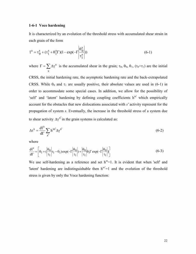
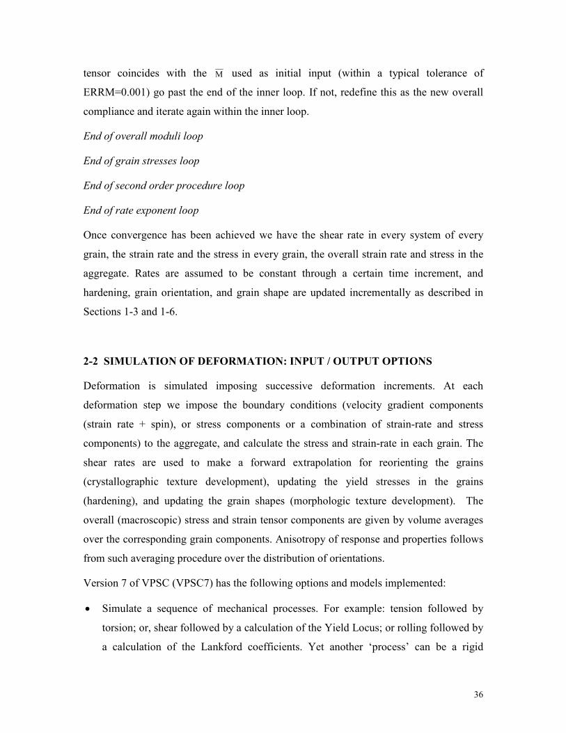
23 0 1 2

0

1

2

3

τ0=1 / τ

1=1 / θ

0=0.2 / θ

1=2

τ(Γ)

τ0=1 / τ

1=1 / θ

0=5 / θ

1=-0.2

τ0=1 / τ

1=-0.5 / θ

0=-5 / θ

1=-0.2

θ1=-0.2θ

0

(τ0+τ

1)

Γ

τ0

0 1 20

1

2

3

τ(Γ)

τ0=1 / τ

1=0 / θ

0=0 / θ

1=0

τ0=1 / τ

1=0 / θ

0=0.2 / θ

1=0.2

τ0=1 / τ

1=1 / θ

0=5 / θ

1=0.2

θ1

θ0

(τ0+τ

1)

Γ

τ0

∆ΓΓτ

=τ∆d

ˆd ss (6-4)

The hardening law described by Eqs. 6-1 to 6-3 permits us to describe the high hardening

rate observed at the onset of plasticity, and its decrease towards a constant hardening rate

at large strains. The condition 0,0 110 ≥τ≥θ≥θ corresponds to increasing yield stress and

decreasing hardening rate tending to linear saturation. Linear hardening is a limit case of

this law corresponding to 0s1 =τ and the case of rigid-perfectly-plastic hardening

corresponds to 0110 =τ=θ=θ (see Figure). The parameters in Eqs. (6-1) and (6-2)

associated with hardening of each slip mode are read from file FILECRYS.

The threshold associated with each system in each grain is updated inside SUBROUTINE

UPDATE_CRSS_VOCE. However, the incremental expression (6-2) represents a

forward extrapolation which tends to overestimate the hardening and make it dependent

on the step size, more so when the

derivative is large. As a consequence, we

have implemented an analytic integration

of Eq. 6-2 inside SUBROUTINE

UPDATE_CRSS_VOCE. The

procedure is described in Appendix C.

Non-kosher Voce hardening: Normally,

the evolution of the threshold stress

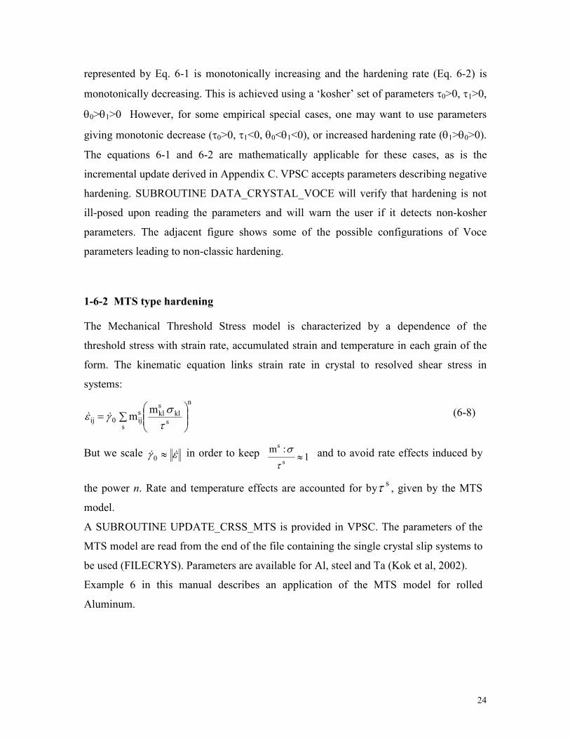
24

represented by Eq. 6-1 is monotonically increasing and the hardening rate (Eq. 6-2) is

monotonically decreasing. This is achieved using a ‘kosher’ set of parameters τ0>0, τ1>0,

θ0>θ1>0 However, for some empirical special cases, one may want to use parameters

giving monotonic decrease (τ0>0, τ1<0, θ0<θ1<0), or increased hardening rate (θ1>θ0>0).

The equations 6-1 and 6-2 are mathematically applicable for these cases, as is the

incremental update derived in Appendix C. VPSC accepts parameters describing negative

hardening. SUBROUTINE DATA_CRYSTAL_VOCE will verify that hardening is not

ill-posed upon reading the parameters and will warn the user if it detects non-kosher

parameters. The adjacent figure shows some of the possible configurations of Voce

parameters leading to non-classic hardening.

1-6-2 MTS type hardening

The Mechanical Threshold Stress model is characterized by a dependence of the

threshold stress with strain rate, accumulated strain and temperature in each grain of the

form. The kinematic equation links strain rate in crystal to resolved shear stress in

systems:

n

skl

skl

s

sij0ij

mm

∑=

τσ

γε ɺɺ (6-8)

But we scale εγ ɺɺ ≈0 in order to keep 1

:m

s

s

≈τ

σ and to avoid rate effects induced by

the power n. Rate and temperature effects are accounted for bysτ , given by the MTS

model.

A SUBROUTINE UPDATE_CRSS_MTS is provided in VPSC. The parameters of the

MTS model are read from the end of the file containing the single crystal slip systems to

be used (FILECRYS). Parameters are available for Al, steel and Ta (Kok et al, 2002).

Example 6 in this manual describes an application of the MTS model for rolled

Aluminum.

25

Crystallographic MTS Model Associated equations and parameters for Ta

Main equation

0

ˆ)T,(S

0

ˆ)T,(S i

ia

µτ

εµτ

εµτ

µτ ε

ε ɺɺ ++=

Where: aτ = 16.46 MPa

Shear modulus vs T

−−=

1)T

Texp(

D1

00

0µµ

Where: µ0 = 62250 MPa

0D = 0.00582MPa

0T = 40 K

Forest independent structure factor

ii

lngb

kT1)T,(S

p/1q/1

i0

i03i

−=εε

µε

ɺ

ɺɺ

Where: i0εɺ = 1x107 s-1

qi = 3/2

pi = 1/2

=ig 0 0.1236

iσ = 495 MPa

Forest related structure factor

εε

εε

µε ε

εε

p/1q/1

0

03

lngb

kT1)T,(S

−=

ɺ

ɺɺ

Where: εε0ɺ = 1x107 s-1

g0ε = 1.6

qε = 1

pε = 2/3

Forest related hardening

κ

ττ

µµ

θετ

ε

εε

−⋅=

v0

0ˆ

ˆ1

d

ˆd

Where: =κ 2.0

0θ =1.479 MPa

Saturation stress vs rate and temperature

=

s0s03

0s

s lngb

kT

ˆ

ˆln

εεε

ε

εε

µττ

ɺ

ɺ

Where: g 0εs = 0.2625

0sετ =144 MPa

s0εεɺ = 1x107 s-1

1-7 TWINNING MODEL

26

While here we assume that twinning has associated, as slip, a critical resolved shear of

activation in the twinning plane and along the twinning direction, it differs from slip in its

directionality, which we model by allowing activation only if the resolved shear stress is

positive (along the Burgers vector of the twin).

Another aspect of twinning that needs to be incorporated into the models is the fact that

the twinned fractions are regions (usually of lamellar morphology) with a different

orientation than the surrounding matrix. These twinned regions not only contribute to the

texture of the aggregate but, most important, act as effective barriers for the propagation

of dislocations or of other twin lamellae. The hardening induced by the twins is

empirically enforced here by assigning high values to the latent hardening coefficients hss'

describing slip-twin and twin-twin interactions.

As for the effect on texture of the twinned fractions, here we use the Predominant Twin

Reorientation Scheme (PTR) proposed by Tomé et al [1991], which works as follows:

within each grain g we keep track of the shear strain g,tγ contributed by each twin system

t, and of the associated volume fraction tg,tg,t S/V γ= as well (St is the characteristic

twin shear). The sum over all twin systems associated with a given twin mode, and over

all grains, represents the 'accumulated twin fraction' Vacc, mode

in the aggregate for the

particular twin mode (the one that one would measure by SEM).

t

g,t

g t

emod,acc

SV γ= ∑∑ (7-1)

Since it is not numerically feasible to consider each twinned fraction as a new orientation,

the PTR scheme adopts a statistical approach. At each incremental step we fully reorient

some grains by twinning provided certain conditions are fulfilled. We call 'effective

twinned fraction' Veff, mode

the volume associated with the fully reoriented grains for that

mode, and define a threshold volume fraction as

emod,acc

emod,eff2th1themod,th

V

VAAV += (7-2)

After each deformation increment we pick a grain at random and identify the twin system

with the highest accumulated volume fraction. If the latter is larger than the threshold

Vth, mode

then the grain is allowed to reorient and Veff, mode

and Vth, mode

are updated. The

27

process is repeated until either all grains are randomly checked or until the effective twin

volume exceeds the accumulated twin volume. In the latter case we stop reorientation by

twinning and proceed to the next deformation step. Two things are achieved in this

process: a) only the historically most active twin system in each grain is considered for

reorienting the whole grain by twinning; b) the twinned fraction is consistent with the

shear activity that the twins contribute to deformation. The algorithm given by Eq. 7-2

prevents grain reorientation by twinning until a threshold value Ath1

is accumulated in

any given system (typically 10-25% of grain volume) and rapidly raises the threshold to a

value around Ath1

+Ath2

(typically 50-60% of grain volume).

The PTR scheme is implemented inside SUBROUTINE UPDATE_TWINNING, and the

user can define different values of Ath1

and Ath2

for each twin mode. These parameters are

read from file FILECRYS and are stored in arrays THRES1 & THRES2. The user has

the option to allow or prevent twin reoriented grains from undergoing a second

reorientation by twinning. Secondary twinning is controlled by ISECTW (=1 allow

retwinning, =0 no retwinning) which is read from FILECRYS for each twin mode.

This feature is also handled inside SUBROUTINE UPDATE_TWINNING.

1-8 SECOND-ORDER FORMULATION

1-8-1 Second-order moments

The effective stress potential TU of a linear ‘thermoelastic’ polycrystal described by Eq.

(5-5) may be written in the form (Liu and Ponte Castañeda, 2004):

( ) G2

1:oE::MU

2

1T +Σ+Σ⊗Σ= (8-1)

where M and oE are calculated by means of Eqs. 5-40 and G is the energy under zero

applied stress a stress potential. Let us rewrite the expressions for M and oE and add the

expression for G as:

∑==r

)r()r()r()r()r( B:McB:MM (8-2)

28

∑ ε=ε+=r

)r()r(o)r()r(o)r()r(o B:cb:ME (8-3)

∑ ε=r

)r()r(o)r( b:cG (8-4)

where )r(c is the volume fraction associated with grain (r).

The average second-order moment of the stress over grain (r) is given by (Liu and Ponte

Castañeda, 2004):

( ))r()r()r()r()r()r()r(

T)r(

)r(

M

G

c

1:

M

oE

c

1::

M

M

c

1

M

U

c

2

∂

∂+Σ

∂

∂+Σ⊗Σ

∂

∂=

∂

∂=σ⊗σ (8-5)

The first derivative in the right term can be obtained solving the following equation [9]:

)uv,r(ij)r(

uv

klijkl

M

Mπ=

∂

∂Ω (8-6)

where ijklΩ and )uv,r(

ijπ are given elsewhere (Lebensohn et al, 2005). Expression (8-6) is

a linear system of 25 equations with 25 unknowns (i.e. the components of )r(uvkl MM ∂∂ ).

In turn, the other two derivatives appearing in Eq. (8-5) can be calculated as:

)r(uv

klikl

)uv,r(i)r(

uv

oi

M

M

M

E

∂

∂ζ+θ=

∂

∂ ,

)r(uv

oi

i)uv,r(

)r(uv M

E

M

G

∂

∂ϑ+η=

∂

∂ (8-7)

where iklζ , iϑ , )uv,r(

iθ and

)uv,r(η are given in Lebensohn et al (2005).

Once the average second moments of the stress are obtained, the corresponding second

moments of the strain-rate can be calculated as follows:

( ) )r(o)r(o)r()r(o)r(o)r()r()r()r()r(::MM ε⊗ε−ε⊗ε+ε⊗ε+σ⊗σ⊗=ε⊗ε (8-8)

(See SUBROUTINE FLUCTUATIONS for details of the implementation of the

calculation of second-order moments).

The above average second moments over grain (r) (Eqs. 8-5 and 8-8) can be used to

generate the average second moment of the equivalent stress and strain-rate in grain (r)

as:

29

2/1)r(

2

3)r(eq ::I

σ⊗σ=σ (8-9a)

2/1)r(

3

2)r(eq ::I

ε⊗ε=ε (8-9b)

The standard deviations of the equivalent magnitudes in grain (r) are defined as:

( ) ( ) ( )2)r(eq

2)r(eqeq

)r(SD σ−σ=σ (8-10a)

( ) ( ) ( )2)r(eq

2)r(eqeq

)r(SD ε−ε=ε (8-10b)

The standard deviations of the equivalent magnitudes over the whole polycrystal are

defined as:

( ) 2eq

2eqeqSD Σ−Σ=σ (8-11a)

( ) 2eq

2eqeq EESD −=ε (8-11b)

where:

( ) ( )∑ σ=σ=Σr

2)r(eq

)r(2)r(eq

2eq c (8-12a)

( ) ( )∑ ε=ε=r

2)r(eq

)r(2)r(eq

2eq cE (8-13b)

It is worth noting that the overall SD’s defined by Eqs. (8-11) are a global scalar

indicators that contain information about both intergranular and intragranular stress and

strain-rate heterogeneity.

(See SUBROUTINE SDPX and output file FLUCT.OUT).

1-8-2 Second-order procedure

30

Once the average second-order moments of the stress field over each grain are obtained

by means of the calculation of the derivatives appearing in Eq. (8-5), the implementation

of the SO procedure follows the work of Liu and Ponte Castañeda (2004). The covariance

tensor of stress fluctuations is given by:

)r()r()r()r(C σ⊗σ−σ⊗σ=σ (8-14)

The average and the average fluctuation of resolved shear stress on slip system (k) of

grain (r) is given by:

)r(k)r()k(

:m σ=τ , ( ) 21k)r(k)r()k(

)r()k(

m:C:mˆ σ±τ=τ (8-15)

where the positive (negative) branch should be selected if )r()k(

τ is positive (negative). The

slip potential of slip system (k) in every grain is defined as:

( )1n

ko

ko

)k(1n

+

τ

τ

+τ

=τφ (8-16)

Two scalar magnitudes associated with each slip system (k) of each grain (r) are defined

by (see SUBROUTINE SOP and arrays ASO and ESO):

( )( )( ) ( )( )

)r()k(

)r()k(

)r()k(

r)k(

)r()k(

r)k(r

)k(ˆ

ˆ

τ−τ

τφ′−τφ′=α ,

( ) ( )( ) )r()k(

)r()k(

)r()k(

r)k(

r)k(

e τα−τφ′= (8-17)

where ( ) ( )ττφ=τφ′ d/d)k()k(

. The linearized local behavior associated with grain (r) is

then given by SO),r(o)r(SO),r()r( :M ε+σ=ε , where (See SUBROUTINE SOMOD):

( )∑ ⊗α=k

kk)r()k(

SO),r(mmM , ∑=ε

k

k)r()k(

SO),r(ome (8-18)

The SO procedure requires iterating over SO),r(

M and SO),r(oε to derive improved

estimations of a linear comparison polycrystal. Each of these polycrystals has associated

31

different first- and second-order moments of the stress field in the grains. These statistical

moments can be used to obtain new values of )r()k(

α and )r()k(

e , which in turn define a new

linear comparison polycrystal, etc. This convergence procedure is terminated when the

input and output values of )r()k(

α and )r()k(

e coincide within a certain tolerance.

1-8-3 Numerical implementation of the SO

Initial guess for )r()k(

α and )r()k(

e :

The above scheme to adjust the values of )r()k(

α and )r()k(

e requires the adoption of initial

guesses for these magnitudes. In the present implementation we adopted the “affine”

guess. From Eq. (43), the “affine” local compliance and back-extrapolated term of grain

(r) are given by:

( )( )

( )kk

knk

o

1n)r(k

oaff),r(

mm:m

nM ⊗τ

σγ= ∑

−

(8-19)

( ) k

k

n

ko

)r(k

oaff),r(o

m:m

n1 ∑

τ

σγ−=ε (8-20)

The “affine” initial guesses for )r()k(

α and )r()k(

e are given by (see SUBROUTINE

GRAIN_RATE_AND_MODULI called by INITIAL_STATE_GUESS)

[ ] ( )( )nk

o

1n)r(k

oo)r(

)k(

:mn

τ

σγ=α

−

(8-21)

[ ] ( )

n

ko

)r(k

oo)r(

)k(

:mn1e

τ

σγ−= (8-22)

‘Incremental’ procedure for low rate-sensitive materials:

32

If a SO calculation should be performed for a low rate sensitive material, the procedure

described above for the adjustment )r()k(

α and )r()k(

e of could fail to converge. In that case,

the convergence could be achieved by using incremental steps in the exponent n.

Typically, it is necessary to: a) obtain converged values of )r()k(

α and )r()k(

e for the first

three values in a sequence of increasing exponents n, b) use those three initial values of

)r()k(

α and )r()k(

e to perform a quadratic interpolation for each of these magnitudes, c)

obtain extrapolated estimations of )r()k(

α and )r()k(

e to be used as initial guesses for the

subsequent exponent in the incremental sequence (see Increasing rate exponent loop: DO

JXRS=JXRSINI, JXRSFIN, JXRSTEP in SUBROUTINE VPSC, and SUBROUTINE

EXTRAPOLSO).

‘Partial’ update of )r()k(

α and )r()k(

e

Since the values of the second moments are strongly dependent on the ‘linear comparison

polycrystal’ (determined by the set of )r()k(

α and )r()k(

e ) and this set of values is obtained

precisely from second moments, it is sometimes necessary to adopt a ‘partial’ update

criterion for iterative adjustment of )r()k(

α and )r()k(

e . For example, if ]i[)r(

)k(α and

]new[)r()k(

α

are, respectively, the current value and the corresponding new estimation of )r()k(

α

obtained by means of Eq. (62), a smooth convergence requires the actual updated value

of )r()k(

α be calculated as: ]new[)r(

)k(]i[)r(

)k(]1i[)r(

)k(3132 α+α=α +

(see SUBROUTINE

FLUCTUATIONS).

33

1-8 REFERENCES

M. Berveiller, O. Fassi-Fehri and A. Hihi, 1987. “The problem of two plastic and

heterogeneous inclusions in an anisotropic medium”. Int. J. Eng. Sci. 25, 691-709.

I.J. Beyerlein, R.A. Lebensohn and C.N. Tomé, "Modeling of texture and

microstructural evolution in the equal channel angular process", Mats. Sc. and

Engineering A345 (2003) 122-138.

O. Engler, M.Y. Huh and C.N. Tomé, 2000. "A study of through-thickness texture

gradients in rolled sheets". Metall. Mater. Trans. 31A, 2299-2315

M.E. Gurtin, 1981. "An Introduction to Continuum Mechanics", Academic Press (San

Diego).

J.W. Hutchinson, 1976. “Bounds and self-consistent estimates for creep of polycrystalline

materials”. Proc. R. Soc. London A 348, 101-121.

G.C. Kaschner, C.N. Tomé, I.J. Beyerlein, S.C. Vogel, D.W. Brown, R.J. McCabe, 2006.

“Role of twinning in the hardening response of Zr during temperature reloads”,

Acta Materialia 54, 2887-96

U.F. Kocks, C.N. Tomé and H.-R. Wenk, 2000. “Texture and Anisotropy”, Cambridge

University Press (2nd

edition).

S. Kok, A.J. Beaudoin and D.A. Tortorelli, 2002. "A polycrystal plasticity model based

on the mechanical threshold", Int. J. Plasticity 18, 715-741.

R.A. Lebensohn and C.N. Tomé, 1993. "A self-consistent anisotropic approach for the

simulation of plastic deformation and texture development of polycrystals -

Application to zirconium alloys", Acta Metall Mater 41 (1993) 2611-2624.

R.A. Lebensohn, D. Solas, G.R. Canova and Y. Brechet, 1996. "Modelling damage of Al-

Zn-Mg alloys". Acta Mater. 44, 315-325.

R.A. Lebensohn, P.A. Turner, J.W. Signorelli, G.R. Canova and C.N. Tomé, 1998a.

"Calculation of intergranular stresses based on a large strain visco-plastic self-

consistent model", Mod. Sim. Mats. Sc. Eng. 6, 447-465.

R.A. Lebensohn, H.-R. Wenk and C.N. Tomé, 1998b. "Modeling deformation and

recrystallization textures in calcite", Acta mater. 46, 2683-2693.

R.A. Lebensohn, C.N. Tomé and P.J. Maudlin, 2003. “An extended self-consistent visco-

plastic formulation: application to polycrystals with voids”. Int. Report of Los

Alamos Natl. Lab. LA-UR-03-1193. (available at

http://www.lanl.gov/mst/voids.shtml).

R.A. Lebensohn, C.N. Tomé and P.J. Maudlin, 2004. “A selfconsistent formulation for

the prediction of the anisotropic behavior of viscoplastic polycrystals with voids”. J.

Mech. Phys. Solids 52, 249-278.

R.A. Lebensohn, C.N. Tomé and P. Ponte Castañeda, 2005. "Improving the self-

consistent predictions of texture development of polycyrystals incorporating

intragranular field fluctuations" Materials Science Forum 495-497, 955-964.

34

Y. Liu and P. Ponte Castañeda. 2004 "Second-order theory for the effective behavior and

field fluctuations in viscoplastic polycrystals. J. Mech. Phys. Solids 52, 467–495.

R. Masson., M. Bornert, P. Suquet and A. Zaoui, 2000. “An affine formulation for the

prediction of the effective properties of nonlinear composites and polycrystals”. J.

Mech. Phys. Solids 48, 1203-1227.

A. Molinari., G.R. Canova and S. Ahzi, 1987. “A self-consistent approach of the large

deformation polycrystal viscoplasticity”. Acta metall. 35, 2983-2994.

Mura T., 1987. Micromechanics of defects in solids (2nd

edition). Martinus Nijhoff

Publishers, Dordrecht, The Netherlands.

C.N. Tomé, 1999. "Self-consistent polycrystal models: a directional compliance criterion

to describe grain interactions ", Mod. Sim. Mats. Sc. Eng. 7, 723-738.

C.N. Tomé, G.R. Canova, U.F. Kocks, N. Christodoulou and J.J. Jonas, 1984."The

relation between macroscopic and microscopic strain hardening in FCC

polycrystals", Acta metall. 32, 1637-1653.

C.N. Tomé and R.A. Lebensohn, 2004. "Self consistent homogeneization methods for

texture and anisotropy", in "Continuum Scale Simulation of Engineering Materials:

Fundamentals, Microstructures, Process Applications", edited by D. Raabe, F.

Roters, F. Barlat and L.Q. Chen, Wiley-VCH Verlag GmbH & Co, KGaA,

Weinheim, pp 473-499.

C.N. Tomé, R. A. Lebensohn and U.F. Kocks, 1991. "A model for texture development

dominated by deformation twinning: application to zirconium alloys", Acta Metall.

Mater. 39, 2667.

C.N. Tomé, R.A. Lebensohn and C.T. Necker, "Anisotropy and orientation correlations

of recrystallized aluminum", Metall. and Materials Transactions 33A (2002) 2635-

48

C.N. Tomé, P.J. Maudlin, R.A. Lebensohn and G.C. Kaschner, 2001. "Mechanical

response of zirconium. Part I: Derivation of a polycrystal constitutive law and Finite

Element analysis", Acta Materialia 49, 3085-96

L.J. Walpole, 1969. On the overall elastic moduli of composite materials, J. Mech. Phys.

Solids 17, 235-251.

35

SECTION 2: DESCRIPTION OF THE VPSC CODE

2-1 NUMERICAL ALGORITHM

The self-consistent algorithm is solved inside SUBROUTINE VPSC. It consists of two

nested iterations. The outer iteration varies the stress (and so the grain compliance) in

each grain. The inner iteration varies the overall viscoplastic moduli of the aggregate.

The previous loops are nested inside two more external loops: the outermost allows for an

incremental variation of the rate sensitivity exponent ‘n’ (not run by default; used to

achieve convergence). The innermost of the two corresponds to the Second Order (SO)

procedure (is only required when running this approximation). When comparing tensors

inside VPSC we calculate the norm of their difference divided by the norm of their

average. This criterion permits to define relative discrepancies and to use always the

same relative tolerance (typically 0.001).

Increasing rate exponent loop: DO N=NRSINI, NRSFIN, NRSTEP

Second order loop: DO ITSO=1, ITMAXSO (or tolerance<ERRSO)

Grain stresses loop: DO IT1=1,ITMAX1 (or tolerance<ERRS & ERRD)

For the first iteration define initial stress guess )r(σ in each grain enforcing an upper-

bound (Taylor) interaction (impose same E)r( =ε in every grain), and define an initial

guess for the overall compliance M as the inverse of the average of the inverse grain

compliances. Define also an initial guess for oE compatible with the latter (Eq 5-5). For

every step calculate in each grain )r(σ (using the interaction equation), and the plastic

compliance (r)M and the back-extrapolated term )r(oε as a function of

)r(σ (Section 1-5-

7).

Overall moduli loop: DO IT2=1,ITMAX2 (or tolerance<ERRM)

1) Calculate Eshelby tensor as a function of M and the ellipsoid axes; 2) Calculate M~

and )r(

B and )r(

b using Eqs.(5-33 to 5-36); 3) Calculate M using Eq.(5-41) and if this

36

tensor coincides with the M used as initial input (within a typical tolerance of

ERRM=0.001) go past the end of the inner loop. If not, redefine this as the new overall

compliance and iterate again within the inner loop.

End of overall moduli loop

End of grain stresses loop

End of second order procedure loop

End of rate exponent loop

Once convergence has been achieved we have the shear rate in every system of every

grain, the strain rate and the stress in every grain, the overall strain rate and stress in the

aggregate. Rates are assumed to be constant through a certain time increment, and

hardening, grain orientation, and grain shape are updated incrementally as described in

Sections 1-3 and 1-6.

2-2 SIMULATION OF DEFORMATION: INPUT / OUTPUT OPTIONS

Deformation is simulated imposing successive deformation increments. At each

deformation step we impose the boundary conditions (velocity gradient components

(strain rate + spin), or stress components or a combination of strain-rate and stress

components) to the aggregate, and calculate the stress and strain-rate in each grain. The

shear rates are used to make a forward extrapolation for reorienting the grains

(crystallographic texture development), updating the yield stresses in the grains

(hardening), and updating the grain shapes (morphologic texture development). The

overall (macroscopic) stress and strain tensor components are given by volume averages

over the corresponding grain components. Anisotropy of response and properties follows

from such averaging procedure over the distribution of orientations.

Version 7 of VPSC (VPSC7) has the following options and models implemented:

• Simulate a sequence of mechanical processes. For example: tension followed by

torsion; or, shear followed by a calculation of the Yield Locus; or rolling followed by

a calculation of the Lankford coefficients. Yet another ‘process’ can be a rigid

37

rotation of the crystallographic texture and the grain morphology, as found in

sequential ECAE routes.

• Mixed boundary conditions (complementary components of stress and velocity

gradient) can be imposed. In particular, creep conditions.

• Twinning modes can be used to accommodate shear, and twinning reorientation is

treated according to the Predominant Twin Reorientation (PTR) scheme described

above.

• Non-reversible slip modes can be used. In this case slip takes place in the sense of the

Burgers vector read from FILECRYS but not in the opposite sense. This feature is

useful for representing non-centro-symmetric slip observed in geologic materials.

Twin shear is treated using this feature.

• Grain reorientation can be 'coupled' to the reorientation of one or more neighbors.

• Evolution of fcc rolling components (Brass, Goss, copper, cube, S, rotated cube) can

be followed during deformation.

• Evolution of individual grain ellipsoid shape and orientation (morphologic texture)

can be followed. Evolution of the average (macroscopic) ellipsoid is always

followed.

• Mixed exponents: slip and twinning systems may have different rate sensitivities

(exponent n).

• Simulate a non-uniform deformation path (parameter IVGVAR=1) by entering a

history of deformation. See description of SUBROUTINE VAR_VEL_GRAD in

following page.

• It is possible to calculate a 2-dim projection of the Polycrystal Yield Surface (PCYS)

declaring IVGVAR=2 in VPSC.IN (requires to enter components of the 2-d

subspace), or to calculate Lankford coefficients between 0 and 90 deg with respect

to. the RD by declaring IVGVAR=3 (requires to provide angular increment for

‘probing’).

• It is possible to save the state of grains and polycrystal corresponding to deformation

step n in a file POSTMORT.OUT by setting ISAVE=n in VPSC.IN, and start a

simulation from POSTMORT.IN by setting IRECOVER=1. By default ISAVE=0

and no postmortem file is written.

38

• It is possible to simulate deformation of a multiphase aggregate. Initial texture and

hardening parameters of each phase are entered through VPSC.IN.

• The code has been adapted for future interfacing with Finite Element codes, to be

used as a material subroutine of the latter. As a consequence, it contains a ‘multi-

element’ option. Note: an FE material subroutine based on VPSC7 has yet to be

developed. The last one available (VPSC5FE) was based on VPSC5.

• The code solves the self-consistent algorithm defined by Eqs. 5-40 or 5-41. It also

allows one to impose the Taylor condition of equal strain increment to every grain.

Note: Relaxed Constraint conditions are not provided in VPSC7. However, RC is a

limit case of the Self Consistent model, when the grain shape becomes highly

distorted.

The input to the code consists in:

• Initial crystallographic texture (grain orientations and weights).

• Single crystal properties (active slip and twinning systems, their critical resolved

shear stresses, and the associated hardening parameters).

• Initial morphological texture (initial grain shapes and shape orientations).

• Boundary conditions (overall velocity gradient components, or overall stress

components. Also temperature if running the MTS model (IHARDLAW=1).

• Parameters controlling convergence, precision and type of run.

• Optional input: strain history, rolling components (CUBCOMP.IN), previous state of

grains (POSTMORT.IN).

The output of the code is:

• Final (optionally intermediate) crystallographic and morphologic textures of each

phase after deformation.

• Evolution of the stress and strain components during deformation.

• Statistics of slip and twinning systems activity during deformation.

• Statistic over grain stress and strain-rate components and their standard deviations.

39

• Optional output: morphologic texture of each phase, rolling components, PCYS scan,

Lankford scan, directional Young modulus, state of grains and polycrystal

(POSTMORT.OUT)

2-3-1 GRAIN SHAPE EVOLUTION OPTIONS

The VPSC model treats each grain as an ellipsoidal inclusion, and explicitly accounts for

individual grain shape and its evolution with strain. As a consequence, VPSC provides a

tool to analyze how grain shape affects slip activity, hardening and texture evolution.

Refer to Section 1.3, describing the connection between grain shape and the deformation

gradient, and to Section 1.5.3, describing the Eshelby tensor. See Beyerlein et al (2003)

for ‘grain fragmentation model’. (Inside the code see implementation in SUBROUTINE

UPDATE_SHAPE)

Under severe plastic deformation grains adopt distorted shapes and extreme aspect ratios,

and tend to rotate with the flow field at a faster rate than equiaxed grains. However, there

are physical and numerical limits to how distorted a grain can become. From a numerical

point of view the evaluation of the integrals associated with the Eshelby tensor (5.27)

becomes less accurate. From a physical point of view, severely distorted grains, are

likely to split into sub-grains. VPSC has two options for dealing with grain shape

evolution:

Option 1 (IFRAG=0): when the ratio between the longest and shortest axes of the

ellipsoid reaches a critical value CRIT_SHP (typically, CRIT_SHP=25), the code

‘freezes’ the shape and stops updating the axes. The ellipsoid is still allowed to rotate

rigidly.

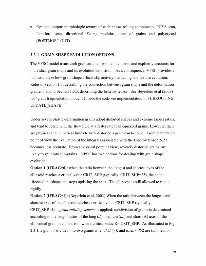
Option 2 (IFRAG=1): (Beyerlein et al, 2003) When the ratio between the longest and

shortest axes of the ellipsoid reaches a critical value CRIT_SHP (typically,

CRIT_SHP=5), a grain splitting scheme is applied: subdivision of grains is determined

according to the length ratios of the long (dl), medium (dm) and short (ds) axes of the

ellipsoidal grain in comparison with a critical value R= CRIT_SHP. As illustrated in Fig.

2.3.1, a grain is divided into two grains when dl/ds > R and dm/ds < R/2 are satisfied, or

40

into four grains when dl/ds > R and dm/ds > R/2. The crystallographic orientation

immediately before and after the split remains the same.

original grain, Vf

L/2

L

Vf/2

M/2

M

(a) Elongated grain, one split

(b) flat ellipsoid, two splits

new grains Vf/4

S

2-3-2 VARIABLE VELOCITY GRADIENT OPTION

It is possible to run a non-uniform deformation path by setting IVGVAR=1 in input file

VPSC7.IN, and providing the path & name of the strain history file. The history file may

correspond to the output for a given element from a Finite Element run, or may be a file

created previously by the user. Under this option the code will call the SUBROUTINE

VAR_VEL_GRAD (VARiable VELocity GRADient) and set the boundary conditions to

‘fully imposed velocity gradient’ (this setting is hardwired but may be changed if

needed). VAR_VEL_GRAD is called at each incremental step and the following

information is read: the 9 components of the velocity gradient UDOT(i,j) and the time

increment TINCR for the step (see file LIJ_HIST.DAT in Example 2, corresponding to

rolling with a superimposed variable shear). Inside VAR_VEL_GRAD the following

magnitudes are calculated and passed to the calling module: the strain rate tensor

DSIM(I,J) (symmetric component of the velocity gradient), and its 5-dimensional vector

representation DBAR(I).

41

2-4 CODE ARCHITECTURE

The modules of the code are: 1) a driver VPSC7.FOR; 2) an array declaration file

VPSC7.DIM; 3) a library of specific plasticity routines VPSC7.SUB; 4) a library of

general numerical routines LIBRARY7.SUB.

1) VPSC7.FOR: Controls the simulation run and the output. Ideally the user should not

need to modify subroutines for performing a specific calculation (such as calculating

Lankford coefficients, or yield surfaces). The opening of I/O units and the unit numbers

are also controlled from this module. At the end of VPSC7.FOR the following two

statements:

INCLUDE VPSC7.SUB

INCLUDE LIBRARY7.SUB

include the subroutines into the main file when compiling the code.

2) VPSC7.DIM: Dimensions arrays to be shared by MAIN and SUBROUTINES in

COMMON declarations. This file is included through a statement:

INCLUDE VPSC7.DIM

which appears in VPSC7.FOR and in most subroutines of VPSC7.SUB.

The user controls dimensions by modifying only this file. Meaningful variables and

arrays (in COMMON areas) are made available through this module for manipulation,

access and output to be done from VPSC7.FOR.

The following parameters are used for dimensioning arrays and have to be defined by the

user. When launched, the code checks the input data against the maximum dimensions

declared and issues a warning if they are exceeded. The actual number of systems,

modes, phases or grains in a particular may be smaller than the dimension declared by the

parameters:

NPHPEL (number of phases per element): maximum number of (crystallographic) phases

in the aggregate. When running the Finite Element material subroutine only one

crystallographic phase can be considered per element.

42

NPHMX (number of phases maximum): maximum number of (crystallographic) phases

in the aggregate or (alternatively) maximum number of elements. The latter applies to a

multi-element run or a finite element application.

NMODMX: maximum number of active slip plus twinning modes in any of the

crystallographic phases.

NSYSMX: maximum number of slip & twinning systems in any of the crystallographic

phases.

NTWMMX: maximum number of twinning modes in any of the crystallographic phases.

NGRMX: maximum number of grains over all the phases in the aggregate (when

NELEM=1) or maximum number of grains over all the elements considered (when

NELEM>1).

NGRPEL: maximum number of grains per element. It represents the grains in the

aggregate independently of whether NELEM=1 or NELEM>1).

NNEIMX: maximum number of neighbors considered in the grain-neighbor interaction

(usually 1).

3) VPSC7.SUB: Library of specific subroutines. A list of them with a brief description

will eventually be included in an Appendix.

4) LIBRARY7.SUB: Algebraic and mathematical subroutines (matrix inversion, linear

systems, eigenvalues and eigenvectors, random number generator, etc) from the

NUMERICAL RECIPES library.

2-5 UNITS, REFERENCE SYSTEM AND CONVENTIONS

Internally, the code works with a 5x1 and 5x5 matrix representation of second and fourth

order tensors, respectively (see Kocks, Tomé and Wenk, Ch. 7, 2000). The convention

used for the matrix representation is controlled by the basis of symmetric tensors defined

inside SUBROUTINE CHG_BASIS. In the current version stress and strain-rate

components are represented using the following ‘vector’ convention:

[ ]121323112233112254321 2,2,2,6/)2(,2/)(),,,,( σσσσ−σ−σσ−σ=σσσσσ

43

The output file STR_STR.OUT gives cartesian components of stress (deviatoric or

Cauchy) and strain rate using the Voigt convention:

[ ]12132333221154321 ,,,,,),,,,( σσσσσσ=σσσσσ

As in any numerical code, units are implicit and the numerical values of all the

parameters and magnitudes have to be consistent. Equation (5-1) indicates that the crystal

strain-rate is in the same units as 0γɺ (i.e. 1/sec). As a consequence, the values of the

imposed overall velocity gradient components UDOT(i) are implicitly assumed to be in

the same units. Equation (5-1) also indicates that the grain stress tensor has to be in the

same units as the threshold stress sτ (i.e. MPa). As a consequence, the calculated

macroscopic stress values will be in the same units. The time increment for each step

(TINCR) has to be in inverse of the strain-rate units (i.e. sec).

A frequent subject of confusion has to do with the set of axes in which texture and

deformation are expressed. The texture is read from an input file containing sets of Euler

angles and their respective volume fractions. These Euler angles represent three

successive rotations required to bring the crystal axes (originally coincident with the

sample axes) to their actual position in the aggregate. As a consequence, the sample axes

to which the texture is referred (i.e.: RD=1, TD=2, ND=3) are the same axes in which the

imposed deformation tensor (UDOT(i,j)) has to be expressed. For example, tension along

the transverse direction of the rolled sheet requires to enforce the component UDOT(2,2).

44

2-6 DESCRIPTION OF INPUT FILES

The information about the run conditions and the paths and names of the various input

files that the code may require are all declared in VPSC7.IN, which may be regarded as

the 'master' input file.

2-6-1 File VPSC7.IN

Contains information about input files, deformation path to be simulated and test

conditions.

Line by Line:

Line 1: number of elements ‘NELEM’ (nelem=1 unless running VPSC7FE).

Line 2: number of crystallographic phases in the aggregate ‘NPH’.

Line 3: relative volume fractions of the phases ‘WPH(1:nph)’.

Follows one block per phase with the information about each phase:

Line 4: reminder.

Line 5: grain morphology control (ISHAPE=0 to 4), grain fragmentation control

(IFRAG), critical grain shape (CRIT_SHP).

a- If ISHAPE=0 : average grain shape (ellipsoid orientation and axes) is assumed for

each grain when calculating the Eshelby tensor. This is the usual setting for ISHAPE.

If ISHAPE=1 : same as before, but keeps track of individual grain ellipsoid evolution,

although they are not used in the simulation.

If ISHAPE=2 : uses individual grain ellipsoids to calculate Eshelby tensors and the

grain-matrix interaction.

If ISHAPE=3 : same as ISHAPE=2 but reads initial grain ellipsoid orientations from

FILEAXES.

If ISHAPE=4 : same as ISHAPE=2 but reads initial grain ellipsoid orientation and

axes from FILEAXES.

b- IFRAG=0 : when the ratio between the longest and shortest axes of the ellipsoid

reaches a critical value CRIT_SHP (typically, CRIT_SHP=25), the code ‘freezes’ the

shape and stops updating the axes. The ellipsoid is still allowed to rotate rigidly.

45

IFRAG=1: when the ratio between the longest and shortest axes of the ellipsoid

reaches a critical value CRIT_SHP (typically, CRIT_SHP=5) a grain splitting scheme

is applied (see description in Section 2.3.1)

c- CRIT_SHP : the ratio between the longest and shortest axes of the ellipsoid defining

the threshold for applying either the ‘grain freeze’ or the ‘grain fragmentation’

criterion.

Line 6: initial length of ellipsoid axes (length1, length2, length3) describing average grain

shape (dummy if ISHAPE=4). Only the ratios matter, and not the absolute values.

Line 7: Euler angles describing the initial position of the average ellipsoid with respect to

the sample axes (dummy if ISHAPE=3,4). Axis1 is assumed to have length1, axis2

to have length2, axis3 to have length3.

Line 8: reminder.

Line 9: name and path of crystallographic texture file FILETEXT.

Line 10: reminder.

Line 11: name and path of single crystal properties file FILECRYS.

Line 12: reminder.

Line 13: name and path of grain morphology file FILEAXES (dummy if ISHAPE=0,1,2).

Tolerance settings for convergence procedures (unless expert, use default):

Line 14: reminder.

Line 15: relative tolerances ERRS, ERRD, ERRM, ERRSO allowed in the convergence

procedures inside SUBROUTINE VPSC7 (see Section 2-1). Typically 0.001..

Line 16: maximum number of iterations ITMAXEXT and ITMAXINT allowed in the

convergence procedure of the loop over grain stress states, and the loop over the overall

modulus. Typically ITMAXEXT=100 and ITMAXINT=25. Also number of iterations

associated with the Second Order loop (typically 25).

Line 17: parameter IRSVAR and related parameters. Controls the outermost loop in

SUBROUTINE VPSC. If IRSVAR=0 (default) the other parameters are ignored.

Line 18: convergence parameter IBCINV. Inside SUBR VPSC solves either Eqs. 5-40

(IBCINV=0) or Eqs. 5-41 (IBCINV=1 this is the default).

46

INPUT/OUTPUT settings for the run (unless expert, use 0 as default parameter):

Line 19: reminder

Line 20: parameter IRECOVER.

If IRECOVER=0 uses Taylor stresses as the initial guess in the first step.

If IRECOVER=1 reads grain and polycrystal states from POSTMORT.IN.

Line 21 parameter ISAVE.

If ISAVE=0 does not write initial state of grains and polycrystal.

If ISAVE=n writes grain and polycrystal states into POSTMORT.OUT for

deformation step n. See EXAMPLE 8 for usage.

Line 22: parameter ICUBCOM.

If ICUBCOM=1 calculates the volume fraction associated with each of the typical fcc

rolling components (copper, cube, Goss, S) for each deformation step. VPSC7 will

look for file CUBCOMP.IN to read orientation of all crystallographically equivalent

components.

If ICUBCOMP=0 skips such calculation.

Line 23: parameter NWRITE controls frequency of texture writing in file

TEX_PHn.OUT. Texture is written every NWRITE incremental steps. If NWRITE=0

(default) texture is written only for the last step.

Parameters controlling modeling conditions for the run (user needs to modify):

Line 24: reminder

Line 25: parameter IHARDLAW.

If IHARDLAW=0 uses the hardening parameters associated with the Voce law.

Parameters are read from file FILECRYS.

If IHARDLAW=1 uses MTS hardening parameters. Parameters are read at the end of

file FILECRYS. Voce parameters are ignored.

If IHARDLAW=2 uses a ‘composite grain’ hardening model, specific to twinning

barriers. This is not an option provided in the distribution version.

Line 26: parameter IRATESENS.

If IRATESENS=1 it allows for the rate sensitivity induced by the power n in Eq. 5-1.

If IRATESENS=0 it scales in Eq. 5-1 to the norm of the macroscopic strain-rate,

47

which has the effect of making the result rate-insensitive.

This option does not affect system activity or texture evolution; only affects the

stress.

Line 27: type of inclusion-matrix INTERACTION to be used. (0:Taylor, 1:affine,

2:secant, 3:neff

=10, 4:tangent, 5: second order). see Sections 1-5-7 and 1-8-3.

Line 28: parameters IUPDORI, IUPDSHP, IUPDHAR.

If the corresponding parameter is =1 (default) updates grain orientation, grain shape

and grain hardening after every incremental step.

If the corresponding parameter =0 it keeps constant the initial orientation, shape or

CRSS throughout the run.

Line 29: parameter NNEIGH.

If NNEIGH=0 it does not couple the reorientation of the grains when updating

orientation. This should be the default.

If NNEIGH=n it couples the reorientation of every grain with the reorientation of ‘n’

neighbors chosen randomly from the discrete texture file (typically NNEIGH=1). The

effect of this coupling is to slow down the evolution of texture during deformation.

The following parameters are best left alone unless expert:

Line 30: parameter IFLU. If IFLU=1 calculates intragranular stress fluctuations inside

grains. Slows down the run considerably. Default is IFLU=0, unless running the Second

Order approximation (INTERACTION=5).

Information about tests to be run (user needs to enter information):

Line 31: reminder.

Line 32: number of sequential tests (i.e.: strain paths, yield surface probes, etc) to be run

in the simulation.

Line 33: reminder.

Each process requires two lines in what follows. The first line declares IVGVAR, the

second line contains information pertinent to the process, as follows:

Line 34-35+: IVGVAR.

* If IVGVAR=0 the code will enforce the same velocity gradient in every step. The

load conditions are read from a PROCESS file: path\name are declared in this line

48

* If IVGVAR=1 the code will call SUBROUTINE VAR_VEL_GRAD at each

deformation step (see description in Section 2-3-2) and read the components of the

velocity gradient UDOT and time increment TINCR from a file (typically, the

deformation history of a given element generated by a FE code) whose path and name

is declared in VPSC7.IN.

* If IVGVAR=2 the code calculates a 2-dimensional projection of the Polycrystal

Yield Surface, by probing the aggregate with strain-rate vectors contained in the

projection subspace. Instead of a PROCESS file the user should provide in this line

the two components (out of the 5 deviatoric components) defining the projection sub-

space (see Section 2-5 and EXAMPLE2).

* If IVGVAR=3 the code calculates the Lankford coefficient by simulating tensile

tests in the (x1,x2) plane of the texture (see EXAMPLE2). Instead of a PROCESS file

the user should provide in this line the angular increment (in degrees) for the tensile

‘probing’, from the RD to the TD.

* If IVGVAR=4 the code rotates rigidly the crystallographic and the morphologic

texture of the grains. An example (see EXAMPLE10) is the simulation of an ECAE

route, where after each pass the sample is rotated and reinserted in the die. The

second line gives the path and name of a file containing the 3x3 rotation matrix to be

used for the rigid rotation (see Section 2-3-3 for description).

Example of file VPSC7.IN (unit=0) (corresponding to EXAMPLE2):

1 number of elements (nelem)

1 number of phases (nph)

1.0 0.0 relative vol. fract. of phases (wph(i))

*INFORMATION ABOUT PHASE #1

0 0 25 grain shape contrl, fragmentn, crit aspect ratio

1.0 1.0 1.0 initial ellipsoid ratios (dummy if ishape=4)

0.0 0.0 0.0 init Eul ang ellips axes (dummy if ishape=3,4)

* name and path of texture file (filetext)

example2\rand500.tex

* name and path of single crystal file (filecrys)

example2\fcc.sx2

* name and path of grain shape file (dummy if ishape=0) (fileaxes)

shape1.100

*PRECISION SETTINGS FOR CONVERGENCE PROCEDURES (default values)

0.001 0.001 0.001 0.001 errs,errd,errm,errso

100 100 25 itmax: max # of iter, external, internal and SO loops

49

0 2 10 2 irsvar & jrsini,jrsfin,jrstep (dummy if irsvar=0)

1 ibcinv (0: don't use <Bc>**-1, 1: use <Bc>**-1 in SC eq)

*INPUT/OUTPUT SETTINGS FOR THE RUN (default is zero)

0 irecover:read grain states from POSTMORT.IN (1) or not (0)?

0 isave: write grain states in POSTMORT.OUT at step 'isave'?

1 icubcomp:calculate fcc rolling components?

0 nwrite (frequency of texture downloads)

*MODELING CONDITIONS FOR THE RUN

0 ihardlaw (0:Voce, 1:MTS, 2:composite grain)

1 iratesens (0:rate insensitive, 1:rate sensitive)

1 interaction (0:FC,1:affine,2:secant,3:neff=10,4:tangent,5:SO)

1 1 1 iupdate: update orient, grain shape, hardening

0 nneigh (0 for no neighbors, 1 for pairs, etc.)

0 iflu (0: don't calc, 1: calc fluctuations)

*NUMBER OF PROCESSES (Lij const; Lij variable; PCYS ;LANKFORD; rigid rotatn)

3

*IVGVAR AND PATH\NAME OF FILE OR STRESS SUBSPACE OR ANGULAR INCREMENT

1

example2\lij_hist.dat

2 ivgvar=2 will calculate PCYS at the end

1 2 --> section of stress space

3 ivgvar=3 will calculate Lankford coefficients at the end

10 --> angular increment for tensile probing

2-6-2-1 MONOTONIC PROCESS file (path & name read from VPSC7.IN)

Contains information about velocity gradient and mechanical test conditions.

Line by line:

Line 1: parameters NSTEPS, ICTRL, CTRLINCR, TEMP:

• NSTEPS: number of incremental deformation steps.

• ICTRL: Type of incremental step imposed to achieve final deformation.

If ICTRL=0 a Von Mises equivalent strain increment is imposed.

If 1<ICTRL<6 one of the strain or stress tensor components is imposed, which

one, depends on the value of IUDOT or ISCAU read below. (Voigt convention

used: 1,2,3,4,5,6 indicate 11,22,33,23,13,12 respectively).

If ICTRL=7 the time increment TINCR is imposed and multiplies the imposed

strain rate tensor to give the strain increment.

• CTRLINCR: Magnitude of increment imposed to achieve final deformation.

If ICTRL=0 the CTRLINCR is the Von Mises strain increment.

50

If 1<ICTRL<6 the CTRLINCR is the increment of the strain tensor component

when a strain component is enforced or the time increment when a stress

component (creep) is enforced.

If ICTRL=7 then CTRLINCR is the time increment. Case of strain rate imposed.

• TEMP: temperature (not used unless running MTS hardening: IHARDLAW=1).

Line 2: reminder.

Lines 3-5: flags IUDOT(3,3) associated with each of the nine components of the velocity

gradient tensor Li,j . The corresponding component is enforced or not when IUDOT(i,j) is

1 or 0 respectively. Three of the non-diagonal components have to be enforced because

the rigid body rotation of the sample is part of the boundary conditions.

Lines 6-8: components of the macroscopic velocity gradient in arbitrary units. All nine

are to be given in order to make an initial guess. Only those with IUDOT=1 are enforced.

Lines 9-11: flags ISCAU(6) associated with each of the six independent components of

the Cauchy stress tensor. The corresponding component is enforced or not when

ISCAU(i) is 1 or 0 respectively. ISCAU and IUDOT have to be complementary.

Lines 12-14: components of the macroscopic Cauchy stress in arbitrary units. Only those

with IUDOT=1 are enforced and need to be given (usually equal to zero for free

surfaces).

Example of process file (the sample below corresponds to EXAMPLE2\ROLLING):

50 3 0.02 298. nsteps ictrl eqincr temp

* boundary conditions

1 1 1 iudot | flag for vel.grad.

1 1 1 | (0:unknown-1:known)

1 1 1 |

|

1.0 0. 0. udot | vel.grad

0. 0. 0. |

0. 0. -1.0 |

|

0 0 0 iscau | flag for Cauchy

0 0 |

0 |

|

0. 0. 0. scauchy | Cauchy stress

0. 0. |

0. |

51

2-6-2-2 VARIABLE PROCESS file (path & name read from VPSC7.IN)

Contains information about velocity gradient components and time increment to be

enforced at each step. In its present version it enforces all the components. See meaning

of parameters in description 2-6-2-1 above

Line 1: parameters NSTEPS, ICTRL, CTRLINCR, TEMP

(CTRLINCR & TEMP are dummy, ICTRL has to be equal to 7)

Line 2: remainder

Line 3+: dummy sequential number, Lij, time increment

51 7 0.02 298. nsteps ictrl eqincr temp

step L11 L12 L13 L21 L22 L23 L31 L32 L33 tincr

1 0.1000E+01 0.0000E+00 0.0000E+00 0.0000E+00 0.0000E+00 0.0E+00 0.0000E+00 0.0E+00 -0.1000E+01 0.2E-01

2 0.1000E+01 0.0000E+00 0.1567E+00 0.0000E+00 0.0000E+00 0.0E+00 0.1567E+00 0.0E+00 -0.1000E+01 0.2E-01

3 0.1000E+01 0.0000E+00 0.3109E+00 0.0000E+00 0.0000E+00 0.0E+00 0.3109E+00 0.0E+00 -0.1000E+01 0.2E-01

4 0.1000E+01 0.0000E+00 0.4602E+00 0.0000E+00 0.0000E+00 0.0E+00 0.4602E+00 0.0E+00 -0.1000E+01 0.2E-01

5 0.1000E+01 0.0000E+00 0.6022E+00 0.0000E+00 0.0000E+00 0.0E+00 0.6022E+00 0.0E+00 -0.1000E+01 0.2E-01

……………………………

2-6-3 File FILETEXT (path & name read from VPSC7.IN)

Contains information about initial crystallographic texture.

Line by Line:

Line 1: dummy.

Line 2: dummy.

Line 3: dummy.

Line 4: first letter of the texture convention being used (Roe, Bunge, Kocks) and the

number of orientations to be read from the file.

Line 5 to end: the three Euler angles defining each orientation, and the associated volume

fraction. They are read using free format.

Example of input texture file FILETEXT (unit=2):

52

AXES OF THE REPRESENTATIVE ELLIPSOID

5.0 1.0 0.2

DISCRETE TEXTURE FROM ODF FILE PT420.ODF (1=axis,2=hoop,3=radious)

B 1144

95.00 5.00 5.00 0.00014528

135.00 5.00 5.00 0.00016130

145.00 5.00 5.00 0.00084955

155.00 5.00 5.00 0.00014641

95.00 15.00 5.00 0.00033814

... ... ... ...

2-6-4 File FILECRYS (path & name read from VPSC7.IN)

Contains information about initial single crystal parameters and deformation modes.

Line by Line:

Line 1: reminder

Line 2: crystal symmetry ‘ICRYST’. Could be CUBIC, HEXAGonal, TRIGOnal,

TETRAgonal, ORTHOtropic, MONOClinic, TRICLinic. Only the first five letters of the

word are read.

Line 3: crystal lattice parameters: relative length (a,b,c) of the unit cell axes, and angles

),,( γβα between the axes.

Line 4: reminder.

Line 5-10: elastic constants of the crystal (Voigt notation). VPSC calculates the Voigt,

Reuss and Self-Consistent elastic constants of the initial texture, and writes them in

RUN_LOG.OUT. Elastic constants are a bonus and do not enter in the plastic simulation.

Line 11: reminder.

Line 12: thermal expansion coefficients of the crystal (Voigt notation). Read but ignored

by VPSC.

Line 13: reminder.

Line 14: total number of deformation modes listed in the file.

Line 15: the number of modes to be used in the calculation ‘NMODES’.

Line 16: the correlative numbers that identify the active modes.

Next follows the information about each mode:

Line 17: a label for the mode.

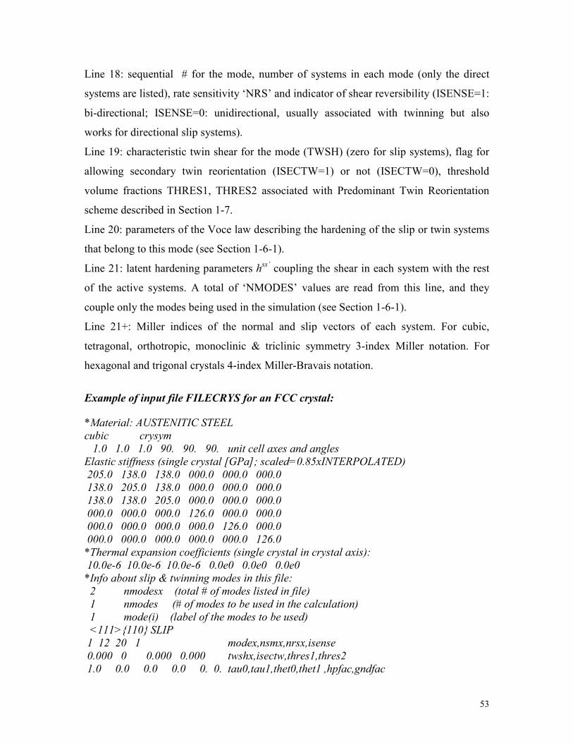
53

Line 18: sequential # for the mode, number of systems in each mode (only the direct

systems are listed), rate sensitivity ‘NRS’ and indicator of shear reversibility (ISENSE=1:

bi-directional; ISENSE=0: unidirectional, usually associated with twinning but also

works for directional slip systems).

Line 19: characteristic twin shear for the mode (TWSH) (zero for slip systems), flag for

allowing secondary twin reorientation (ISECTW=1) or not (ISECTW=0), threshold

volume fractions THRES1, THRES2 associated with Predominant Twin Reorientation

scheme described in Section 1-7.

Line 20: parameters of the Voce law describing the hardening of the slip or twin systems

that belong to this mode (see Section 1-6-1).

Line 21: latent hardening parameters hss’ coupling the shear in each system with the rest

of the active systems. A total of ‘NMODES’ values are read from this line, and they

couple only the modes being used in the simulation (see Section 1-6-1).

Line 21+: Miller indices of the normal and slip vectors of each system. For cubic,

tetragonal, orthotropic, monoclinic & triclinic symmetry 3-index Miller notation. For

hexagonal and trigonal crystals 4-index Miller-Bravais notation.

Example of input file FILECRYS for an FCC crystal:

*Material: AUSTENITIC STEEL

cubic crysym

1.0 1.0 1.0 90. 90. 90. unit cell axes and angles

Elastic stiffness (single crystal [GPa]; scaled=0.85xINTERPOLATED)

205.0 138.0 138.0 000.0 000.0 000.0

138.0 205.0 138.0 000.0 000.0 000.0

138.0 138.0 205.0 000.0 000.0 000.0

000.0 000.0 000.0 126.0 000.0 000.0

000.0 000.0 000.0 000.0 126.0 000.0

000.0 000.0 000.0 000.0 000.0 126.0

*Thermal expansion coefficients (single crystal in crystal axis):

10.0e-6 10.0e-6 10.0e-6 0.0e0 0.0e0 0.0e0

*Info about slip & twinning modes in this file:

2 nmodesx (total # of modes listed in file)

1 nmodes (# of modes to be used in the calculation)

1 mode(i) (label of the modes to be used)

<111>110 SLIP

1 12 20 1 modex,nsmx,nrsx,isense

0.000 0 0.000 0.000 twshx,isectw,thres1,thres2

1.0 0.0 0.0 0.0 0. 0. tau0,tau1,thet0,thet1 ,hpfac,gndfac

54

1.0 1.0 hlat(nmodes)

1 1 1 0 1 -1

1 1 1 1 0 -1

1 1 1 1 -1 0

-1 1 1 0 1 -1

-1 1 1 1 0 1

-1 1 1 1 1 0

-1 -1 1 0 1 1

-1 -1 1 1 0 1

-1 -1 1 1 -1 0

1 -1 1 0 1 1

1 -1 1 1 0 -1

1 -1 1 1 1 0

<111>112 TWIN

2 12 20 0 modex,nsmx,nrsx,isense

0.707 0 0.100 0.500 twshx,isectw,thres1,thres2

1.0 0.0 0.0 0.0 0. 0. tau0,tau1,thet0,thet1 ,hpfac,gndfac

1.0 1.0 hlat(nmodes)

1 1 1 -2 1 1

1 1 1 1 -2 1

1 1 1 1 1 -2

-1 1 1 2 1 1

-1 1 1 -1 -2 1

-1 1 1 -1 1 -2

-1 -1 1 2 -1 1

-1 -1 1 -1 2 1

-1 -1 1 -1 -1 -2

1 -1 1 -2 -1 1

1 -1 1 1 2 1

1 -1 1 1 -1 -2

55

2-7 DESCRIPTION OF OUTPUT FILES

All output files have the extension *.OUT. Most output files are opened inside

VPSC7.FOR for easier control by the user. All the input/output units are defined inside

VPSC7.FOR.

2-7-1 Log file RUN_LOG.OUT (unit=10)

Contains input data read by the code. Provides the Voigt, Reuss and Self-Consistent

elastic constants of the initial aggregate. If some WRITE statements are activated inside

subroutines it also provides information about selected grains.

2-7-2 Optional output file PCYS.OUT (unit=14)

Gets written if IVGVAR=2. Contains the two cartesian coordinates of the 5-dim stress

vector and the strain-rate states associated with a 2-dim projection of the Polycrystal

Yield Surface. The user is prompted to choose two dimensions (i & j) of the 5

dimensional deviatoric space. Plot of Si vs Sj gives the desired projection. The usual π-

plane representation is obtained plotting S2 vs S1 (see EXAMPLE2 and EXAMPLE5).

The probing is done inside SUBROUTINE PCYS using normalized strain rate vectors εɺ

and calculating the associated stress σ . Both tensors are renormalized to εɺ and σ , such

as to give the same dissipation rate for every point of the yield surface, namely: k k 1ε σ =ɺ

S1 S2 D1 D2

0.3712E+00 0.8931E+01 -0.5489E-04 0.1000E+01

0.9334E+00 0.8784E+01 0.1760E+00 0.9984E+00

0.1691E+01 0.8484E+01 0.3572E+00 0.9820E+00

0.3766E+01 0.7483E+01 0.5341E+00 0.9253E+00

0.7736E+01 0.4803E+01 0.6634E+00 0.7918E+00

0.8186E+01 0.4257E+01 0.7595E+00 0.6384E+00

. . .

2-7-3 Optional output file LANKFORD.OUT (unit=15)

Gets written if IVGVAR=3. For each ‘probe’ angle (with respect to the RD) gives the

directional Young modulus, the Lankford coefficient (ratio between in-plane strain-rate

D22 and through-thickness strain-rate D33), the diagonal strain rate components induced

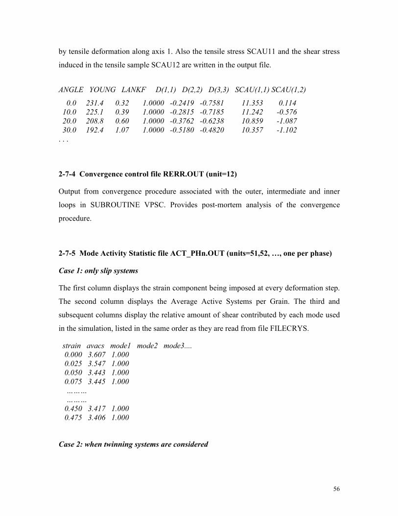
56

by tensile deformation along axis 1. Also the tensile stress SCAU11 and the shear stress

induced in the tensile sample SCAU12 are written in the output file.

ANGLE YOUNG LANKF D(1,1) D(2,2) D(3,3) SCAU(1,1) SCAU(1,2)

0.0 231.4 0.32 1.0000 -0.2419 -0.7581 11.353 0.114

10.0 225.1 0.39 1.0000 -0.2815 -0.7185 11.242 -0.576

20.0 208.8 0.60 1.0000 -0.3762 -0.6238 10.859 -1.087

30.0 192.4 1.07 1.0000 -0.5180 -0.4820 10.357 -1.102

. . .

2-7-4 Convergence control file RERR.OUT (unit=12)

Output from convergence procedure associated with the outer, intermediate and inner

loops in SUBROUTINE VPSC. Provides post-mortem analysis of the convergence

procedure.

2-7-5 Mode Activity Statistic file ACT_PHn.OUT (units=51,52, …, one per phase)

Case 1: only slip systems

The first column displays the strain component being imposed at every deformation step.

The second column displays the Average Active Systems per Grain. The third and

subsequent columns display the relative amount of shear contributed by each mode used

in the simulation, listed in the same order as they are read from file FILECRYS.

strain avacs mode1 mode2 mode3....

0.000 3.607 1.000

0.025 3.547 1.000

0.050 3.443 1.000

0.075 3.445 1.000

………

………

0.450 3.417 1.000

0.475 3.406 1.000

Case 2: when twinning systems are considered

57

The first column displays the strain component being imposed at every deformation step.

The second column displays the Average Active Systems per Grain. The third and fourth

columns display the volume fraction associated with primary twin reoriented grains and

with secondary twin reoriented grains. The following columns display the relative

amount of shear contributed by each mode used in the simulation for each step. The

following columns display the Accumulated Twin Fraction and the Effective Twin

Fraction for each of the twinning modes. When the aggregate is formed by more than one

phase all the above information is displayed for each of the phases separately.

STRAIN AVACS PRITW SECTW MODE1 MODE2 MODE3 MODE4 TWFR3 EFFR3 TWFR4 EFFR4

0.000 2.960 0.000 0.000 0.090 0.000 0.004 0.906 0.000 0.000 0.000 0.000

0.002 2.951 0.000 0.000 0.089 0.000 0.004 0.907 0.000 0.000 0.023 0.000

………………………………………….

0.220 3.303 0.593 0.000 0.237 0.000 0.620 0.143 1.655 0.004 0.588 0.588

2-7-6 Overall statistics file STATS.OUT (unit=11)

Displays general statistics at every incremental step. Most of it is commented out. What

is presently displayed is: the standard deviation with respect to the average of the 5

components of strain rate and stress, expressed in the basis of symmetric tensors (matrix

representation), (normalized with the norm of the strain-rate or the stress, respectively).

epsacu sdev1 sdev2 sdev3 sdev4 sdev5 ddev1 ddev2 ddev3 ddev4 ddev5

0.000 0.101 0.151 0.147 0.160 0.147 0.147 0.240 0.169 0.207 0.169

0.020 0.102 0.147 0.146 0.161 0.152 0.141 0.230 0.166 0.204 0.169

0.040 0.101 0.142 0.139 0.155 0.151 0.144 0.234 0.168 0.206 0.174

… … … … … …

0.980 0.159 0.090 0.075 0.062 0.231 0.054 0.077 0.101 0.373 0.192

1.000 0.161 0.090 0.075 0.061 0.235 0.053 0.074 0.100 0.376 0.192

2-7-7 Stress-strain file STR_STR.OUT (unit=13)

Contains 14 columns with the following information for each deformation step: First two

columns give the overall Von Mises strain and the Von Mises stress. Next six columns

give the six component of the accumulated strain tensor (E11, E22, E33, E23, E13, E12).

58

Next six columns give the six components of the deviatoric stress tensor (S11, S22, S33,

S23, S13, S12) or the six components of the Cauchy stress tensor when the boundary

conditions imposed permit to infer the pressure (i.e.: axial compression test).

Evm Svm E11 E22 E33 E23 E31 E12

SDEV11 SDEV22 SDEV33 SDEV23 SDEV13 SDEV12

0.0000E+00 0.2706E+01 0.000E+00 0.000E+00 0.000E+00 0.000E+00 0.000E+00 0.000E+00 -

0.180E+01 0.929E+00 0.875E+00 0.356E-02 -0.124E-02 -0.941E-02

0.2500E-01 0.4357E+01 -0.250E-01 0.125E-01 0.125E-01 0.000E+00 0.000E+00 0.000E+00 -

0.290E+01 0.149E+01 0.141E+01 0.142E-01 -0.621E-02 -0.169E-01

…………………

…………………

0.4498E+00 0.3292E+02 -0.450E+00 0.225E+00 0.225E+00 0.000E+00 0.000E+00 0.000E+00 -

0.219E+02 0.115E+02 0.104E+02 -0.251E+00 -0.286E+00 -0.105E+00

0.4748E+00 0.3482E+02 -0.475E+00 0.238E+00 0.238E+00 0.000E+00 0.000E+00 0.000E+00 -

0.232E+02 0.122E+02 0.110E+02 -0.283E+00 -0.308E+00 -0.945E-01

2-7-8 Final state in grains and PX file POSTMORT.OUT (unit=19)

Contains the distortion, constitutive moduli, stress of the polycrystal for the particular

step at which it was downloaded. Also contains the stress, the CRSS of every system, the

Euler angles and the accumulated shear in every grain. If appropriate, also contains

information about twinning fractions in each grain and in each phase. The

POSTMORT.OUT file is used to continue a run along the same path or along a different

deformation path, accounting for grain shape, hardening and orientation. For using it as

initial state in a subsequent run it has to be renamed POSTMORT.IN. The option to open

and read it is controlled by the parameter IRECOVER=1 defined inside VPSC7.IN. This

file was originally intended for running sequential strain path changes. Since VPSC7

allows to do sequential deformation histories in one run, now this file is not so relevant.

2-7-9 Output texture files TEX_PHn.OUT or TEX_ELn.OUT (units=31, 32 ….)

One texture file for each of the phases in the aggregate, or for each aggregate (element).

The format is the same as the input texture file FILETEXT. It describes the crystal

orientations with respect to the sample axes, and also gives the volume fraction of each

orientation. The first 3 lines represent a heading. The fourth line contains a ‘B’ for Bunge

convention and the number of orientations in the file. The following lines list, for each

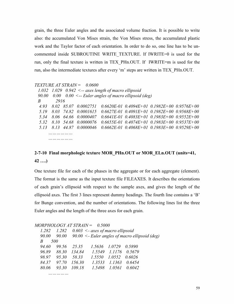
59

grain, the three Euler angles and the associated volume fraction. It is possible to write

also: the accumulated Von Mises strain, the Von Mises stress, the accumulated plastic

work and the Taylor factor of each orientation. In order to do so, one line has to be un-

commented inside SUBROUTINE WRITE_TEXTURE. If IWRITE=0 is used for the

run, only the final texture is written in TEX_PHn.OUT. If IWRITE=m is used for the

run, also the intermediate textures after every ‘m’ steps are written in TEX_PHn.OUT.

TEXTURE AT STRAIN = 0.0600

1.032 1.029 0.942 <-- axes length of macro ellipsoid

90.00 0.00 0.00 <-- Euler angles of macro ellipsoid (deg)

B 2916

4.93 8.02 85.07 0.0002751 0.6620E-01 0.4094E+01 0.1982E+00 0.9576E+00

5.19 8.03 74.82 0.0001615 0.6627E-01 0.4091E+01 0.1982E+00 0.9568E+00

5.34 8.06 64.66 0.0000407 0.6641E-01 0.4083E+01 0.1983E+00 0.9552E+00

5.32 8.10 54.68 0.0000076 0.6655E-01 0.4074E+01 0.1983E+00 0.9537E+00

5.13 8.13 44.87 0.0000046 0.6662E-01 0.4068E+01 0.1983E+00 0.9529E+00

………………

………………

2-7-10 Final morphologic texture MOR_PHn.OUT or MOR_ELn.OUT (units=41,

42 ….)

One texture file for each of the phases in the aggregate or for each aggregate (element).

The format is the same as the input texture file FILEAXES. It describes the orientations

of each grain’s ellipsoid with respect to the sample axes, and gives the length of the

ellipsoid axes. The first 3 lines represent dummy headings. The fourth line contains a ‘B’

for Bunge convention, and the number of orientations. The following lines list the three

Euler angles and the length of the three axes for each grain.

MORPHOLOGY AT STRAIN = 0.5000

1.282 1.282 0.603 <- axes of macro ellipsoid

90.00 90.00 90.00 <- Euler angles of macro ellipsoid (deg)

B 500

94.60 99.56 25.35 1.5636 1.0729 0.5890

96.89 88.30 134.84 1.5549 1.1176 0.5679

98.97 95.30 58.33 1.5550 1.0552 0.6026

84.37 97.70 156.30 1.3533 1.1363 0.6454

80.06 93.30 109.18 1.5498 1.0561 0.6042

……………

60

……………

2-7-11 Rolling components for each phase CUBCOMPn.OUT (units=61, 62 ….)

One file for each of the phases in the aggregate or for each aggregate (element). Each

line gives the current accumulated deformation and the volume fraction of each cubic

rolling component: Balance, COPPER, BRASS, S, GOSS, CUBE , ROTATED CUBE

and the average misorientation.

EPS OTH CU BR S GOS CUB ROT AVMISO

0.0100 53.8 6.6 6.5 14.1 2.7 6.9 9.3 16.1

0.0200 53.8 6.6 6.7 13.9 2.7 6.9 9.3 16.1

0.0300 53.7 6.6 6.7 14.0 2.8 6.9 9.3 16.1

…………………

…………………

0.1500 52.4 4.2 10.3 12.1 3.5 6.9 10.6 16.3

0.1600 52.8 3.8 10.6 11.7 3.6 6.9 10.6 16.3

2-7-12 Convergence control file for the second-order procedure SO.OUT (unit=97)

Output from convergence procedure associated with the rate exponent and second-order

loops in SUBROUTINE VPSC. The relative errors ERRASO and ERRESO are

calculated as averages of the relative errors of the two scalar magnitudes defined per

system and per grain (see Eq. 8-17). It is written only if INTERACTION=5.

2-7-13 Average fluctuations and SD per grain FLUCT.OUT (unit=83)

This file contains the equivalent stress and strain-rate first-order moments (average

values), second-order moments (average field fluctuations, Eqs. 8-9) and Standard

Deviations (SD) (Eqs. 8-10) in every grain, plus the values of the overall SDs

(inter+intragranular) (Eq. 8-11), and intergranular only (inter), after every deformation

step. It is written only when IFLUCT=1.

STEP = 1

NRS = 3

61

GR# SEQ1 SEQ2 SDSEQ DEQ1 DEQ2 SDDEQ

1 0.639E-01 0.104E+00 1.272 0.147E-07 0.224E-07 1.693

2 0.729E-01 0.114E+00 1.350 0.156E-07 0.225E-07 1.623

. . .

499 0.665E-01 0.105E+00 1.253 0.141E-07 0.221E-07 1.706

500 0.971E-01 0.126E+00 1.229 0.622E-08 0.181E-07 1.706

S SDPX (inter+intra) = 1.511

S SDPX (inter) = 0.771

D SDPX (inter+intra) = 1.836

D SDPX (inter) = 0.766

62

2-8 INTERFACING VPSC WITH FINITE ELEMENT CODES outdated

Section!

In order to be able to run several aggregates simultaneously (each one associated with

one element of a FE mesh), we implemented a version of VPSC7 in which the arrays and

the subroutines are minimized. This version consists of a driver named VPSC7FE.FOR,

which plays the role of VPSC7.FOR in the stand-alone version. This driver calls a subset

of the VPSC7 subroutines called VPSC7FE.SUB, which are INCLUDED at the end of

the file. The numerical subroutines in LIBRARY7.SUB are also INCLUDED. This driver

us uses a reduced form of the COMMON statements file, named VPSC7FE.DIM.

The strategy is to use the multi-phase capability of the code, assign the grains associated

with each phase inside each FE element to different 'phases'. By assigning pointers to the

grains belonging to each phase inside each element we can enforce an arbitrary load

history to each element, and carry all internal calculations for each element

independently.

2-8-1 File VPSC7FE.FOR

This driver is a stand-alone application designed to test the multi-element calculation.

The user will have to modify it in order to interface it with his FE code of choice. Please

check comments inside the file for guidance. Internally, this driver calls a SUBROUTINE

VPSC_FE passing the following arguments:

CALL VPSC_FE (INPUT, INITIALIZE, IELEM, TEMP)

• INPUT=.true. instructs the code to open and read the input files containing initial

texture and crystallographic system information, and to copy them into every element

(we assume that initially all elements have the same texture and the same multi-phase

composition). This has to be the first call to VPSC_FE, and for subsequent calls

INPUT should be set to .false.

• INITIALIZE: it has to be set to .true. for the first deformation step imposed to each

element. It enforces an initial Taylor guess for the stress in each grain, in order to

initiate the iterative procedure. Alternatively, it directs the code to use a stress value

for each grain which corresponds to a previous deformation state, and which has been

63

read from POSTMORT.IN if directed to do so inside VPSC7.IN. After VPSC_FE has

been called once for all elements INITIALIZE has to be set to .false.

• IELEM: Is the number that identifies each element in the FE grid. Internally it is used

to identify the grains associated with the aggregate assigned to such element. These

grains are assigned the tags NGR1 to NGR2, and DO LOOPS inside the code will run

between these two limits when solving for element IELEM.

• TEMP: Is the temperature associated with the element. Presently it is used only if the

MTS hardening model is run. TEMP is updated because of adiabatic heating inside

the SUBROUTINE UPDATE_CRSS_MTS, which returns a changed value for TEMP

(unless the user comments out the last three lines, in which case adiabatic heating is

suppressed and TEMP is left unchanged).

The following polycrystal arrays have to be stored after each step because they are used

as starting values when the next strain increment is imposed to the element:

• SAVELE (5,NELEM) : deviatoric stress (S)

• XMTGELE (5,5,NELEM) : tangent compliance (Mtg

)

• XLTGELE (5,5,NELEM) : tangent stiffness (L=M-1

)

• DZEROELE (5,NELEM) : independent term in the constitutive law D=Mtg

:S+D0

• TEMPELE (NELEM) : temperature of the element

The symmetric component of the velocity gradient UDOT(3,3) imposed to the element

has to be copied into DSIM(3,3) and it is passed to VPSC_FE through a COMMON. The

element arrays of the previous step are copied into SAV(5), XMTG(5,5), XLTG(5,5),

DZERO(5) and are passed through a COMMON. They have to be saved when exiting

VPSC_FE.

IMPORTANT: All tensors and the texture used by VPSC are referred to element axes.

The FE code has to keep track of the relative position of the element with respect to

absolute reference system. This includes accounting for the rigid body rotation of the

element (that is why only the symmetric component of the velocity gradient is passed to

VPSC_FE).

64

In the stand-alone application we run a certain number of elements (three) independently

and simultaneously for a number of deformation steps (typically 30), and impose to each

element a different monotonic velocity gradient. This information is read from separate

process files, one for each element. In a real FE application the velocity gradient for each

element will be passed by the calling program, rather than being read from a file.

2-8-2 Input Files

We use the same input files as for VPSC7 (see description in Section 2.6). Only the

differences are addressed in what follows.

VPSC7.IN: The number of FE elements has to be declared in the first line. Differs from

VPSC7 in that, at the end of the file, instead of reading the number and type of processes

to be applied sequentially to the aggregate, VPSC7FE reads the number of elements and

the process file (deformation history) to be applied to each element.

FILETEXT: Initial texture of the elements. Path and name read from VPSC7.IN

FILECRYS: Active slip and twinning systems. Hardening parameters. Path and name

read from VPSC7.IN.

FILEPROC (process file): differs from the VPSC7 process files because VPSC7FE

assumes that all components of the velocity gradient are imposed (this is not necessary

but reflects the way a FE calculation is run). The first line (# of steps, component

controlled, component increment, temperature) is the same. The following lines (in

groups of three) contain the 9 components of the velocity gradient UDOT(i,j) for every

step in the process. Follows an example of tension along axis 1:

15 1 0.01 76 nsteps ictrl eqincr temp

0.001 0. 0.

0. -0.0009 0.

0. 0. -0.0001

0.001 0. 0.

0. -0.0009 0.

0. 0. -0.0001

65

0.001 0. 0.

0. -0.0009 0.

0. 0. -0.0001

……………

……………

POSTMORT.IN: A file POSTMORT.OUT containing the final state of each element and

of every grain in the element gets written at the end of every run. Rename it to

POSTMORT.IN and set IRECOVER=1 inside VPSC7.IN if you want to restart the run

from this state.

2-8-3 OUTPUT FILES

VPSC7FE.OUT: this is a log file meant for the stand-alone application only. It contains

some relevant magnitudes (such as VonMises stress and strain, average grain shape, etc)

for each element and for each step.

STR_STR.OUT: this is a log file meant for plotting and associated with the stand-alone

application only. It contains Von Mises stress and strain for each element and for each

step.

ELEn_PHi.TEX: several files, giving the final texture for each phase ‘i’ in each element

‘n’. The user can dump the texture of any FE element 'ielem', at any step of the

simulation by calling the subroutine WRITE_TEXTURE_FE (IELEM, EVM) from the

driver.

POSTMORT.OUT: contains the final state of each element and of every grain in the

element. It can be written at any step of the simulation by calling the subroutine

POSTMORTEM_FE (2) from the driver. Rename this output file POSTMORT.IN if you

want to use it as input for a subsequent run.

66

SECTION 3: EXAMPLES AND APPLICATIONS

In this Section we describe several application examples for which we provide the

INPUT and the OUTPUT files. These examples illustrate the capabilities of VPSC, and

the characteristics of the interaction approaches implemented in the code. These

examples should be useful both, for testing the installation of the code, and for becoming

acquainted with INPUT files and procedures corresponding to different loading

conditions and material properties. Input files VPSC7.IN, initial texture, single crystal

parameters, and process files are given in all cases. Output files with final texture, stress-

strain history, statistics and activity are also included.

Examples #1 to #6 correspond to cubic aggregates. Example #7 corresponds to an HCP

aggregate deforming by slip and twinning. Example #8 corresponds to orthotropic

olivine, a geological material with less than 5 independent slip systems. Example #9

applies to (hexagonal) ice, and shows how the Second Order formulation deals with a

material with mostly one active deformation mode (basal).

The associated I/O files are stored in separate directories labeled EXAMPLEn. The files

themselves have the same name as described in the manual, but the extension identifies

the different cases considered in the example. For example VPSC7.INb and TEX_PH1.b

are the input file VPSC7.IN and the output file TEX_PH1.OUT, corresponding to Case b.

EXAMPLE 1: Tension and compression of FCC

This simple example is meant to familiarize the user with a basic simulation of texture

evolution, and to visualize the difference that the interaction assumption makes in the

response of the material. For experimental textures and a more comprehensive analysis of

the modeling results see T&A, Chapter 5, Section 1.1, and T&A, Chapter 11, Section 5.1.

Run conditions:

• Random texture file with 500 orientations (file RAND500.TEX).

• FCC crystal with slip on (111)<110> and no hardening: Voce parameters

0,0,0,1 1010 =θ=θ=τ=τ (file FCC.SX). The rate sensitivity parameter is n=20.

67

• Axial tension and compression along x3 up to ε33=100%. All velocity gradient

components are imposed (files TENSION.3 & COMPRE.3).

The results are illustrated in terms of inverse pole figures, showing the tensile or

compressive axis in the crystal reference frame (Figure 1-1) and the stress-strain response

and the slip system activity as a function of the deformation strain (Figure 1-2).

The simulations were done using: the Full Constraints approach (INTERACTION=0), the

affine formulation (INTERACTION=1), the secant formulation (neff

=1,

INTERACTION=2), an intermediate grain-medium interaction (neff

=10,

INTERACTION=3), the tangent formulation (neff

=20, INTERACTION=4), and the

Second Order formulation (INTERACTION=5).

The output files provided are: stress vs strain (STR_STR.*), activity of slip systems

(ACT_PH1.*) and final texture (TEX_PH1.*). The extension identifies tension (t) or

compression (c) plus the particular interaction approach used (0-6). For example

TEX_PH1.c3 is the texture after 100% compression using INTERACTION=3.

It is evident that the different approximations predict differences in final texture, stress

evolution and system activity. The secant case represents a stiff grain-matrix interaction,

and is close to the upper bound represented by the full constraints case (infinitely stiff).

The more compliant cases, tangent and second order, are more efficient in

accommodating deformation and closer to a lower bound: they require less active systems

per grain because grains tend to deform by plane (as opposed to axial) strain, and they

also require lower yield stress. The affine case and neff

=10 give results between the upper

and lower bounds, and their predictions are probably more realistic. The more relevant

consequence of the SC formalism is that for compression it correctly predicts that the

compressive axis tends to align with the <110> crystal direction, a result that the full

constraints formulation fails to predict: the maximum predicted by the FC model is

shifted away from such direction (see Fig 1-1).

68

AFFINE n=10 TANSECFC

(111)

(110)(001) 1

2

4

8

16

32(111)

(110)(001)

Figure 1-1: Inverse pole figure of the tensile axis (top) and the compressive axis (bottom)

after 100% strain. Simulations were done using: Full Constraints (FC), affine, secant

(SEC), neff

=10, and tangent (TAN) in the interaction equation. In all cases n=20 in the

visco-plastic law.

69

0.0 0.5 1.0

2.5

3.0

TENSION

stress

0.0 0.5 1.0

COMPRESSION

0.0 0.5 1.0

0

2

4

6

8

slip activity

s tra in0.0 0.5 1.0

Taylor

affine

secant

neff=10

tangent

2nd ord

s tra in

Figure 1-2: Evolution of stress and Average Active Systems per Grain during tensile and

compressive deformation of FCC polycrystal up to 100% strain. See also caption to

Figure 1-1.

70

EXAMPLE 2: Rolling of FCC

This example is meant to familiarize the user with the simulation of sequential processes

and the rolling ‘capabilities’ of VPSC7. Rolling (plane strain) to 63% reduction is

followed by a calculation of the Polycrystal Yield Surface, and a calculation of Lankford

coefficients and directional Young modulus. The evolution of the characteristic rolling

components is also provided.

In addition there is a simulation of non-uniform deformation path (variable shear

superimposed to plane strain) using the SUBROUTINE VAR_VEL_GRAD.

For experimental textures and a more comprehensive discussion see Kocks et al (Chapter

5, Section 1.2) (2000), and Engler et al (2000).

Run conditions:

• Initial random texture file RAND500.TEX with 500 orientations.

• FCC crystals with slip on (111)<110> and linear hardening 1,1,0,1 1010 =θ=θ=τ=τ

(file FCC.SX2).

• Rolling up to ε33=100%. All velocity gradient components are imposed (file

ROLLING).

• Linearization used: INTERACTION=3 (Neff=10)

Case A:

Plane strain deformation (rolling), followed by a calculation of a π-plane projection of the

Polycrystal Yield Surface corresponding to ε33=100%, followed by a calculation of the

Lankford coefficients and the directional Young moduli in the plane of the sheet.

Corresponding data is reported in files TEX_PH1.a, PCYS.a and LANKFORD.a. In

addition, setting ICUBCOMP=1 allows us to calculate the evolution of several texture

rolling components (Goss, cube, copper, etc) with deformation (see file CUBCOMP1.a).

For calculating the π-plane projection of the PCYS set IVGVAR=2 and choose stress

components #1 and #2 inside VPSC7.IN. The calculation of the Lankford coefficients

71

requires to declare IVGVAR=3 in VPSC7.IN. The tensile ‘probing’ is done at angular

increments of 10° between the RD and the TD.

The linear hardening used in this example will not affect the final texture, or the Lankford

coefficient, or the shape of the PCYS. Only the scale of the PCYS is affected.

Case B:

Same as Case A, but superimposing a shear/reverse shear component to the plane strain

deformation (udot13 = udot31 = 1.25*sin(2πε33) ). The velocity gradient imposed at each

step is read inside SUBROUTINE VAR_VEL_GRA from the input file LIJ_HIT.DAT,

which contains the successive component of the velocity gradient and the time

increments. See format below:

51 7 0.02 298. nsteps ictrl eqincr temp

step L11 L12 L13 L21 L22 L23 L31 L32 L33 tincr

1 0.1000E+01 0.0000E+00 0.0000E+00 0.0000E+00 0.0000E+00 0.0E+00 0.0000E+00 0.0E+00 -0.1000E+01 0.2E-01

2 0.1000E+01 0.0000E+00 0.1567E+00 0.0000E+00 0.0000E+00 0.0E+00 0.1567E+00 0.0E+00 -0.1000E+01 0.2E-01

3 0.1000E+01 0.0000E+00 0.3109E+00 0.0000E+00 0.0000E+00 0.0E+00 0.3109E+00 0.0E+00 -0.1000E+01 0.2E-01

4 0.1000E+01 0.0000E+00 0.4602E+00 0.0000E+00 0.0000E+00 0.0E+00 0.4602E+00 0.0E+00 -0.1000E+01 0.2E-01

5 0.1000E+01 0.0000E+00 0.6022E+00 0.0000E+00 0.0000E+00 0.0E+00 0.6022E+00 0.0E+00 -0.1000E+01 0.2E-01

……………………………

Texture, π-plane projection of the Yield Surface, and Lankford coefficients vs angle are

calculated for the 100% rolled aggregate, and reported in files TEX_PH1.b, PCYS.b and

LANKFORD.b. The evolution of the rolling components is also plotted and listed in file

CUBCOMP1.b.

Observe in Fig 2-1 that the shear component breaks the orthotropic symmetry of the

texture. Figure 2-2 shows that it also affects the formability properties of the rolled sheet,

which now exhibits Lankford coefficients below one for every angle.

72

RD RD RD

(100) (110) (111)

(100) (110) (111)

plane stra in + shear

plane stra in

SIMULATED ROLLING OF FCC (63% reduction)

0.7

1.0

1.4

2.0

2.8

4.0

5.6

8.0

11.

Figure 2-1: Simulated final textures after 63% rolling reduction. (a) enforcing plane

strain; (b) superimposing a shear/reverse shear component to the plane strain component.

-10 0 10

-10

0

10

0 30 60 90

0

1

2

3

0.0 0.5 1.0

0

10

20

30

40

-10 0 10

-10

0

10

0 30 60 90

0

1

2

3

0.0 0.5 1.0

0

10

20

30

40

σ22

σ33

σ11

Lankford

Lankford

Cu

brass

S

Goss

cube

%

RD α TD

160

180

200

220

240

Young [GPa]

σ22

σ33

σ11

Lankford

160

180

200

220

240

%

RD α TD

73

Figure 2-2: Polycrystal Yield Surface, Lankford coefficient, directional elastic Young

modulus associated with plane strain (63% rolling reduction), and plain strain + shear.

Also shown is the evolution of the FCC ideal rolling components of the texture.

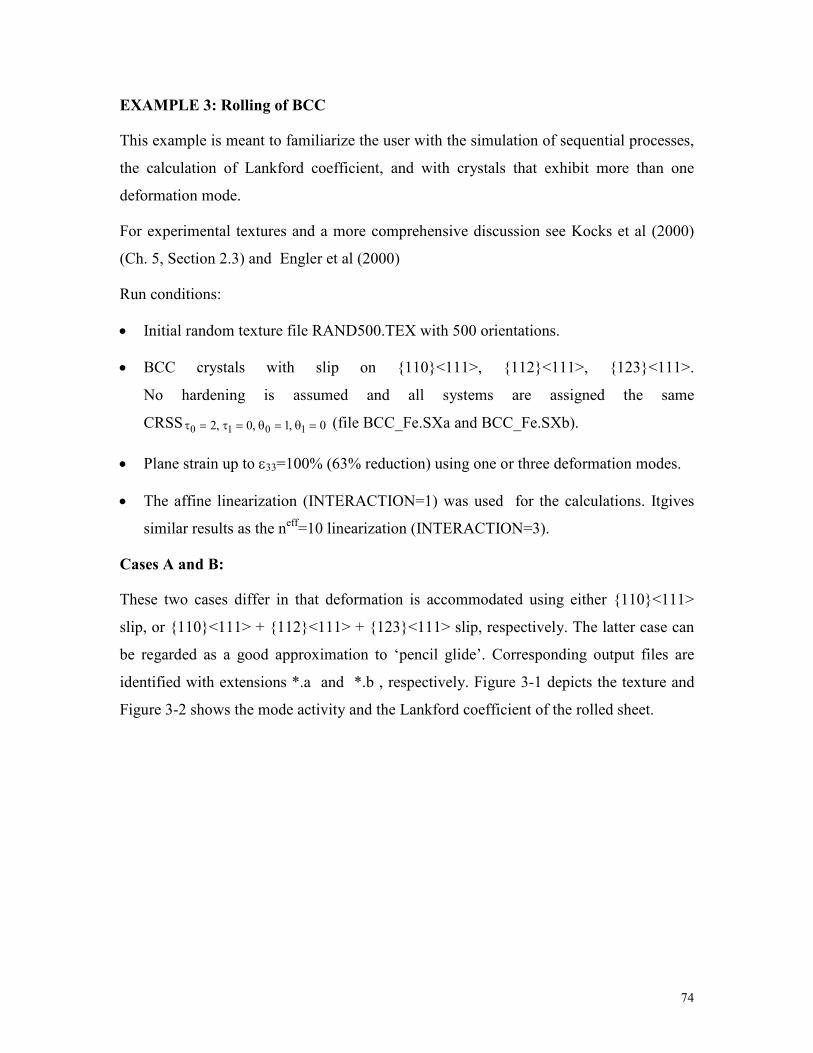
74

EXAMPLE 3: Rolling of BCC

This example is meant to familiarize the user with the simulation of sequential processes,

the calculation of Lankford coefficient, and with crystals that exhibit more than one

deformation mode.

For experimental textures and a more comprehensive discussion see Kocks et al (2000)

(Ch. 5, Section 2.3) and Engler et al (2000)

Run conditions:

• Initial random texture file RAND500.TEX with 500 orientations.

• BCC crystals with slip on 110<111>, 112<111>, 123<111>.

No hardening is assumed and all systems are assigned the same

CRSS 0,1,0,2 1010 =θ=θ=τ=τ (file BCC_Fe.SXa and BCC_Fe.SXb).

• Plane strain up to ε33=100% (63% reduction) using one or three deformation modes.

• The affine linearization (INTERACTION=1) was used for the calculations. Itgives

similar results as the neff

=10 linearization (INTERACTION=3).

Cases A and B:

These two cases differ in that deformation is accommodated using either 110<111>

slip, or 110<111> + 112<111> + 123<111> slip, respectively. The latter case can

be regarded as a good approximation to ‘pencil glide’. Corresponding output files are

identified with extensions *.a and *.b , respectively. Figure 3-1 depicts the texture and

Figure 3-2 shows the mode activity and the Lankford coefficient of the rolled sheet.

75

RD RD RD(100) (110) (111)

RD RD RD

0.6

1.5

3.0

5.0

9.0

15.0

simulated: 110<111> slip

simulated: pencil glide (3 modes)

ROLLING OF BCC (63% reduction)

(100) (110) (111)

RD RD RD

experimental texture

(100) (110) (111)

Figure 3-1: Texture of BCC after 63% rolling reduction. Simulations assume either 110

<111> slip, or 110<111> + 112<111> + 123<111> slip (pencil glide).

0.0 0.5 1.0

0.0

0.5

1.0MODE ACTIVITY

110<111>

112<111>

123<111>

relative activity

strain

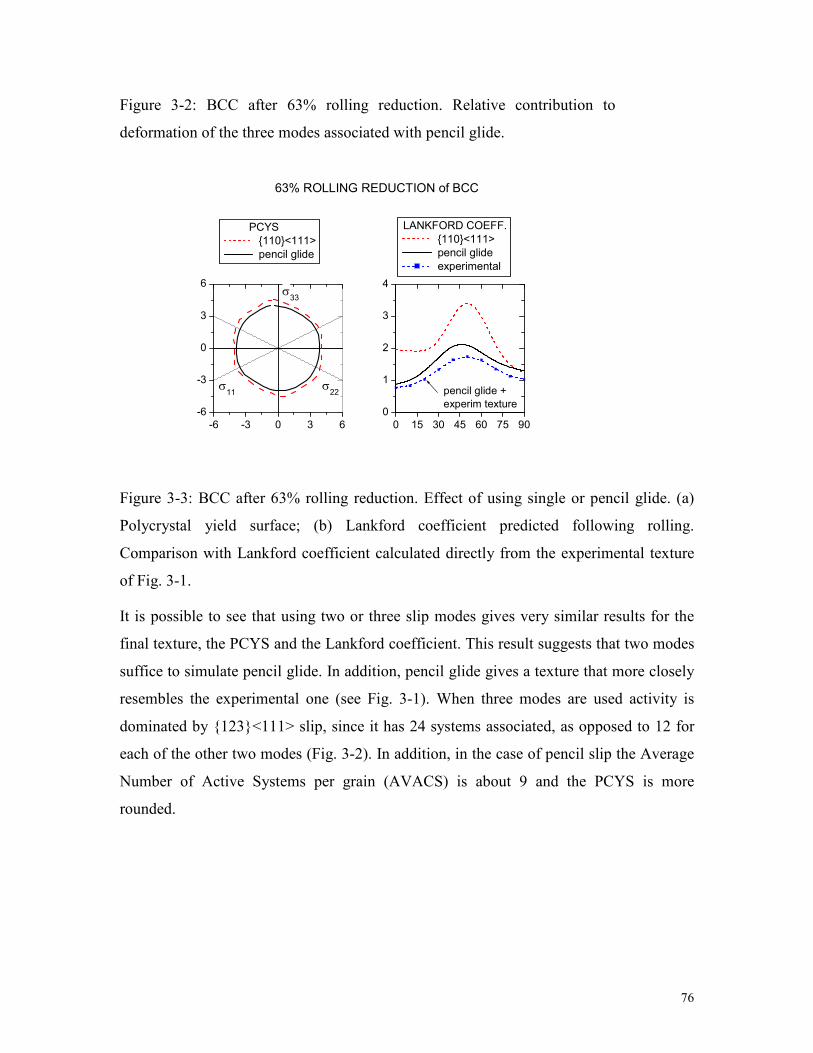
76

Figure 3-2: BCC after 63% rolling reduction. Relative contribution to

deformation of the three modes associated with pencil glide.

0 15 30 45 60 75 90

0

1

2

3

4

-6 -3 0 3 6

-6

-3

0

3

6

PCYS

110<111>

pencil glide

pencil glide +

experim texture

63% ROLLING REDUCTION of BCC

LANKFORD COEFF.

110<111>

pencil glide

experimental

σ22

σ33

σ11

Figure 3-3: BCC after 63% rolling reduction. Effect of using single or pencil glide. (a)

Polycrystal yield surface; (b) Lankford coefficient predicted following rolling.

Comparison with Lankford coefficient calculated directly from the experimental texture

of Fig. 3-1.

It is possible to see that using two or three slip modes gives very similar results for the

final texture, the PCYS and the Lankford coefficient. This result suggests that two modes

suffice to simulate pencil glide. In addition, pencil glide gives a texture that more closely

resembles the experimental one (see Fig. 3-1). When three modes are used activity is

dominated by 123<111> slip, since it has 24 systems associated, as opposed to 12 for

each of the other two modes (Fig. 3-2). In addition, in the case of pencil slip the Average

Number of Active Systems per grain (AVACS) is about 9 and the PCYS is more

rounded.

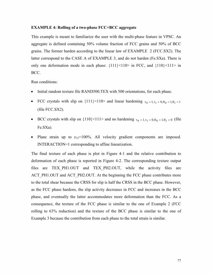
77

EXAMPLE 4: Rolling of a two-phase FCC+BCC aggregate

This example is meant to familiarize the user with the multi-phase feature in VPSC. An

aggregate is defined containing 50% volume fraction of FCC grains and 50% of BCC

grains. The former harden according to the linear law of EXAMPLE 2 (FCC.SX2). The

latter correspond to the CASE A of EXAMPLE 3, and do not harden (Fe.SXa). There is

only one deformation mode in each phase: 111<110> in FCC, and 110<111> in

BCC.

Run conditions:

• Initial random texture file RAND500.TEX with 500 orientations, for each phase.

• FCC crystals with slip on 111<110> and linear hardening 1,1,0,1 1010 =θ=θ=τ=τ

(file FCC.SX2).

• BCC crystals with slip on 110<111> and no hardening 0,1,0,1 1010 =θ=θ=τ=τ (file

Fe.SXa).

• Plane strain up to ε33=100%. All velocity gradient components are imposed.

INTERACTION=1 corresponding to affine linearization.

The final texture of each phase is plot in Figure 4-1 and the relative contribution to

deformation of each phase is reported in Figure 4-2. The corresponding texture output

files are TEX_PH1.OUT and TEX_PH2.OUT, while the activity files are

ACT_PH1.OUT and ACT_PH2.OUT. At the beginning the FCC phase contributes more

to the total shear because the CRSS for slip is half the CRSS in the BCC phase. However,

as the FCC phase hardens, the slip activity decreases in FCC and increases in the BCC

phase, and eventually the latter accommodates more deformation than the FCC. As a

consequence, the texture of the FCC phase is similar to the one of Example 2 (FCC

rolling to 63% reduction) and the texture of the BCC phase is similar to the one of

Example 3 because the contribution from each phase to the total strain is similar.

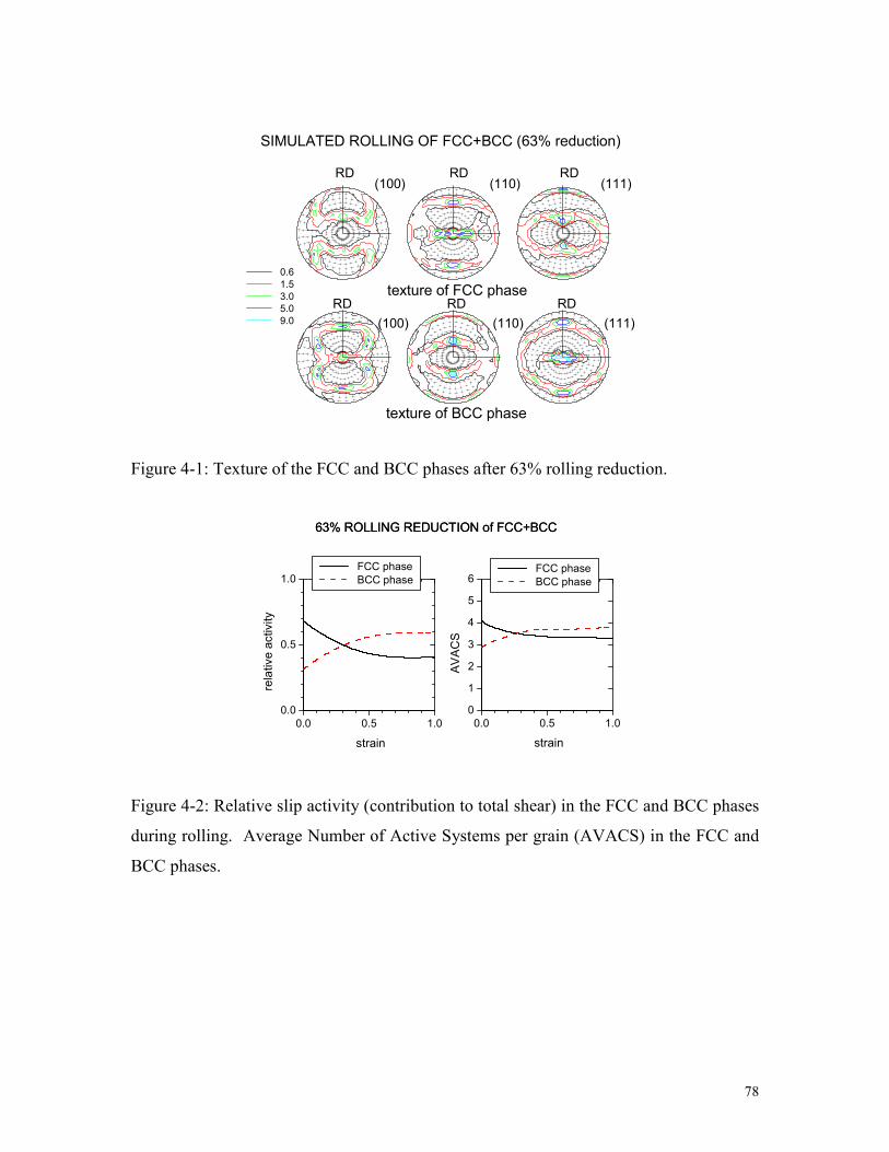
78

0.6

1.5

3.0

5.0

9.0

RD RD RD

(100) (110) (111)

(100) (110) (111)RD RD RD

texture of BCC phase

texture of FCC phase

SIMULATED ROLLING OF FCC+BCC (63% reduction)

Figure 4-1: Texture of the FCC and BCC phases after 63% rolling reduction.

0.0 0.5 1.0

0.0

0.5

1.0

0.0 0.5 1.0

0

1

2

3

4

5

6 FCC phase

BCC phase

63% ROLLING REDUCTION of FCC+BCC

relative activity

strain

FCC phase

BCC phase

63% ROLLING REDUCTION of FCC+BCC

AVACS

strain

Figure 4-2: Relative slip activity (contribution to total shear) in the FCC and BCC phases

during rolling. Average Number of Active Systems per grain (AVACS) in the FCC and

BCC phases.

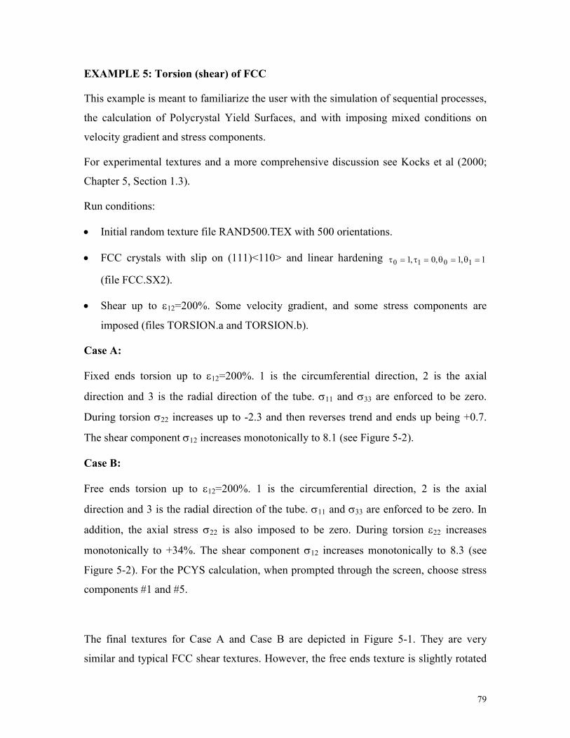
79

EXAMPLE 5: Torsion (shear) of FCC

This example is meant to familiarize the user with the simulation of sequential processes,

the calculation of Polycrystal Yield Surfaces, and with imposing mixed conditions on

velocity gradient and stress components.

For experimental textures and a more comprehensive discussion see Kocks et al (2000;

Chapter 5, Section 1.3).

Run conditions:

• Initial random texture file RAND500.TEX with 500 orientations.

• FCC crystals with slip on (111)<110> and linear hardening 1,1,0,1 1010 =θ=θ=τ=τ

(file FCC.SX2).

• Shear up to ε12=200%. Some velocity gradient, and some stress components are

imposed (files TORSION.a and TORSION.b).

Case A:

Fixed ends torsion up to ε12=200%. 1 is the circumferential direction, 2 is the axial

direction and 3 is the radial direction of the tube. σ11 and σ33 are enforced to be zero.

During torsion σ22 increases up to -2.3 and then reverses trend and ends up being +0.7.

The shear component σ12 increases monotonically to 8.1 (see Figure 5-2).

Case B:

Free ends torsion up to ε12=200%. 1 is the circumferential direction, 2 is the axial

direction and 3 is the radial direction of the tube. σ11 and σ33 are enforced to be zero. In

addition, the axial stress σ22 is also imposed to be zero. During torsion ε22 increases

monotonically to +34%. The shear component σ12 increases monotonically to 8.3 (see

Figure 5-2). For the PCYS calculation, when prompted through the screen, choose stress

components #1 and #5.

The final textures for Case A and Case B are depicted in Figure 5-1. They are very

similar and typical FCC shear textures. However, the free ends texture is slightly rotated

80

clockwise with respect to the fixed end texture. Such difference is what leads to the

development of an axial strain component. The situation is clearly illustrated by the

PCYS in Figure 5-2. Observe that at ε12=100% , the normal to the PCYS at the

intersection with the σ22 axis has a marked positive component. Such component tends

to disappear when ε12=200%.

TORSION TEXTURES AT ε12=1 & ε

12=2

2 2

11

0.7

1.0

1.4

2.0

4.0

8.0

(111) (111)

FREE END TORSION

FIX END TORSION

2 2

11 (111) (111)

Figure 5-1: (111) pole figures associated with fix-end and free-end torsion testing.

-15 -10 -5 0 5 10 15

-15

-10

-5

0

5

10

15

0.0 0.5 1.0 1.5 2.0

0

5

fix end

ε12=1

ε12=2

σ22

σ12

fix end

ε22=0 ε

22

σ22

σ12

stress

ε12

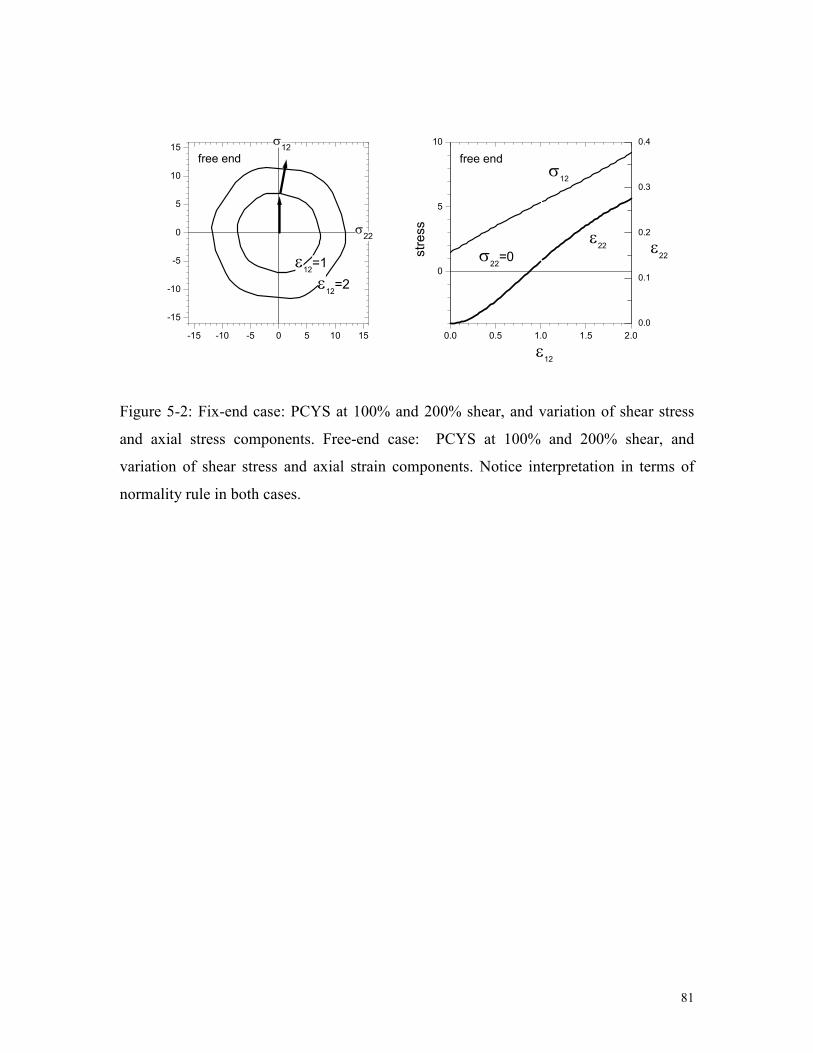
81

-15 -10 -5 0 5 10 15

-15

-10

-5

0

5

10

15

0.0 0.5 1.0 1.5 2.0

0

5

10

free end

ε12=1

ε12=2

σ22

σ12

free end

ε22 ε

22σ22=0

σ12

stress

ε12

0.0

0.1

0.2

0.3

0.4

Figure 5-2: Fix-end case: PCYS at 100% and 200% shear, and variation of shear stress

and axial stress components. Free-end case: PCYS at 100% and 200% shear, and

variation of shear stress and axial strain components. Notice interpretation in terms of

normality rule in both cases.

82

EXAMPLE 6: Application of MTS model to rolled aluminum

This example is the only one in the manual where we use the MTS hardening model

described in Section 6-2. This application compares evolution of yield stress during

compression, at different temperature and/or rates. It includes a simulation of strain-rate

jump.

Run conditions:

• Mesured initial texture of a rolled cold-strip aluminum (file Al_ROLL.TEX 956

orientations). Directions 1,2,3 correspond to RD,TD,ND.

• FCC crystals with slip on (111)<110> and MTS parameters adjusted to reproduce

experimental compression results by Kok et al (2002) (file Al_5182.SX).

• Uniaxial compression up to ε11=30% along the RD. σ11 and σ22 are enforced to be

zero. The following conditions are simulated:

Reference: T=298K at a rate of 10-3

s-1

. File COMP_RF1.30

High temp: T=598K at a rate of 10-3

s-1

. File COMP_HT1.30

High rate: T=298K at a rate of 103 s

-1 . File COMP_HR1.30

Mix rates: T=298K, 15% at 10-3

s-1

, 15% at 103 s

-1 . Files COMP_RF1.15 and

COMP_HR1.15

The texture of the initial and compressed material is depicted in Figure 6-1. The stress-

strain response is given in Figure 6-2.

Case A:

A file VPSC7.INa is provided. The user has to replace the proper ‘process’ file at the end

in order to reproduce the data. Those files are COMP_RF1.30, COMP_HT1.30, and

COMP_HR1.30

The initial texture is depicted in Fig 6-1 (a) and the 30% compression texture in Fig. 6-1

(b). Rate or temperature conditions do not affect the texture development.

The stress is clearly much lower at 598K, and much higher at 103s

-1 (see Fig. 6-2)

Case B:

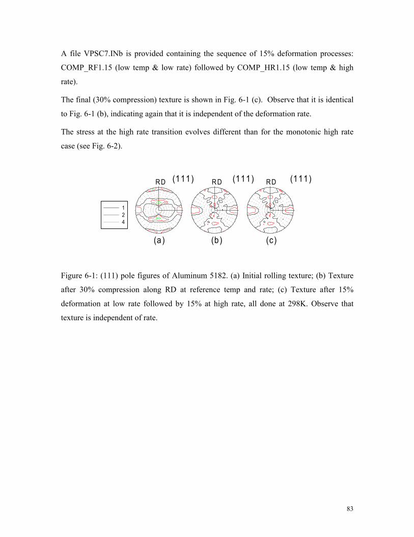
83

A file VPSC7.INb is provided containing the sequence of 15% deformation processes:

COMP_RF1.15 (low temp & low rate) followed by COMP_HR1.15 (low temp & high

rate).

The final (30% compression) texture is shown in Fig. 6-1 (c). Observe that it is identical

to Fig. 6-1 (b), indicating again that it is independent of the deformation rate.

The stress at the high rate transition evolves different than for the monotonic high rate

case (see Fig. 6-2).

(a) (b) (c)

RD RD RD(111) (111) (111)

1

2

4

Figure 6-1: (111) pole figures of Aluminum 5182. (a) Initial rolling texture; (b) Texture

after 30% compression along RD at reference temp and rate; (c) Texture after 15%

deformation at low rate followed by 15% at high rate, all done at 298K. Observe that

texture is independent of rate.

84

0.0 0.1 0.2 0.3

0

100

200

300

400

500

600

700

800

Y Axis Title

X Axis T itle

298K / 10-3s-1

298K / 103s-1

598K / 10-3s-1

298K / 10-3 to 10

3s-1

Figure 6-2: Macroscopic hardening of AA5182 in compression along RD, predicted by

the MTS model, for different loading conditions discussed in the text.

85

EXAMPLE 7: Twinning and anisotropy of HCP Zr

Zirconium is an HCP metal below about 900 K. This example is meant to familiarize the

user with a system which exhibits slip and twinning deformation modes, and which is

highly anisotropic both, at the single crystal and polycrystal level. This is the only

example in this manual where twinning is considered. Twinning is treated using the

Predominant Twin Reorientation scheme described in Section 7.1. Hardening is treated

with the extended Voce law and latent hardening parameters that empirically account for

the barrier effect of twins upon dislocations or other twins.

In this example we use the constitutive law for Zr at room temperature reported by

Kaschner et al (2006). The parameters are reported in Table 7.1 below. We also report the

parameters for liquid nitrogen temperature (76K) but do not provide examples. These

parameters are slightly different from the ones reported by Tomé et al (2000): the

difference reflects a different Zr batch and modifications made in the treatment of

hardening since 2000.

Run conditions:

• Initial texture ( Zr_5678.TEX) is represented using 1944 orientations and corresponds

to clock-rolled and annealed Zr plate with a strong basal component (hard) along the

ND (direction 3) of the plate (see Fig. 7.1).

• HCP crystals deform by (10-10)<11-20> prismatic <a> slip, (10-11)<11-23>

pyramidal <c+a> slip and (10-12)<11-23> tensile twinning at room temperature. We

include (11-22)<11-2-3> compressive twins in the calculation, although their

hardening parameters are such that they do not contribute to deformation at 293K.

The single crystal hardening parameters (file Zr_293K.SX) were adjusted to

experimental tensile and compression data. We also provide the 76K parameters in

file Zr_76K.SX. See Table 7.1 below.

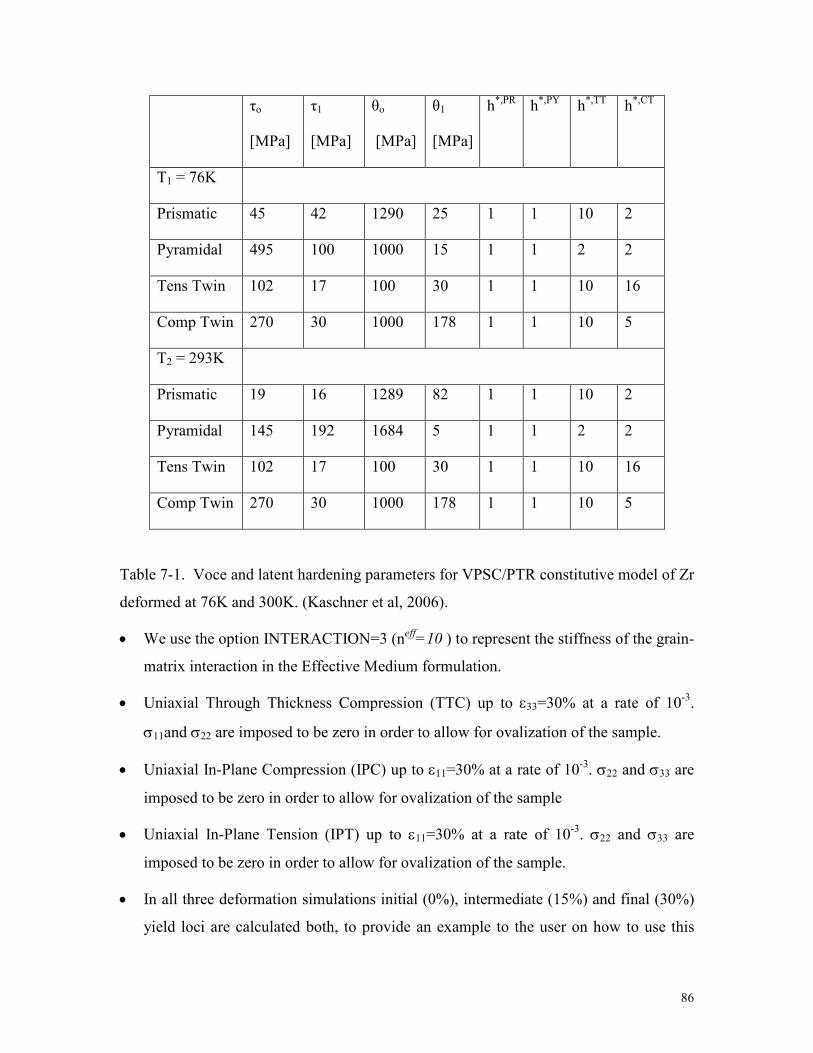
86

τo

[MPa]

τ1

[MPa]

θo

[MPa]

θ1

[MPa]

h*,PR

h*,PY

h*,TT

h*,CT

T1 = 76K

Prismatic 45 42 1290 25 1 1 10 2

Pyramidal 495 100 1000 15 1 1 2 2

Tens Twin 102 17 100 30 1 1 10 16

Comp Twin 270 30 1000 178 1 1 10 5

T2 = 293K

Prismatic 19 16 1289 82 1 1 10 2

Pyramidal 145 192 1684 5 1 1 2 2

Tens Twin 102 17 100 30 1 1 10 16

Comp Twin 270 30 1000 178 1 1 10 5

Table 7-1. Voce and latent hardening parameters for VPSC/PTR constitutive model of Zr

deformed at 76K and 300K. (Kaschner et al, 2006).

• We use the option INTERACTION=3 (neff=10 ) to represent the stiffness of the grain-

matrix interaction in the Effective Medium formulation.

• Uniaxial Through Thickness Compression (TTC) up to ε33=30% at a rate of 10-3

.

σ11and σ22 are imposed to be zero in order to allow for ovalization of the sample.

• Uniaxial In-Plane Compression (IPC) up to ε11=30% at a rate of 10-3

. σ22 and σ33 are

imposed to be zero in order to allow for ovalization of the sample

• Uniaxial In-Plane Tension (IPT) up to ε11=30% at a rate of 10-3

. σ22 and σ33 are

imposed to be zero in order to allow for ovalization of the sample.

• In all three deformation simulations initial (0%), intermediate (15%) and final (30%)

yield loci are calculated both, to provide an example to the user on how to use this

87

VPSC code feature, and to show the effect of twinning upon the yield surface. Only

π-plane projections, corresponding to the subspace

[ ]6/)2(,2/)(),( 112233112221 σ−σ−σσ−σ=σσ ,are calculated (see Section 2.5)

THROUGH THICKNESS COMPRESSION

2 (0002)(0002)

1

2

30%15%0 %

2 (0002)

IN PLANE COMPRESSION2 (0002)(0002)

1

2

30%15%0 %

0.7

1.0

1.4

2.0

2.8

4.0

5.6

2

IN PLANE TENSION

2 (0002)(0002)

1

2

30%15%0 %

2 (0002)

Figure 7-1: (0002) basal pole figures. Initial (0%) and predicted deformation textures of

clock-rolled Zr after 15% and 30% deformation in Through Thickness Compression, In-

Plane Compression and In-Plane Tension (referred to plate axes).

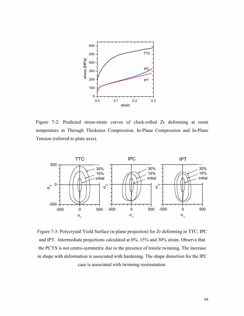
88

0.0 0.1 0.2 0.3

0

100

200

300

400

500

600

IPT

IPC

TTC

stress [MPa]

strain

Figure 7-2: Predicted stress-strain curves of clock-rolled Zr deforming at room

temperature in Through Thickness Compression, In-Plane Compression and In-Plane

Tension (referred to plate axes).

-500 0 500

-500

0

500

TTC

σ2

σ1

30%

15%

initial

-500 0 500

IPC

σ2

σ1

30%

15%

initial

-500 0 500

IPTσ2

σ1

30%

15%

initial

Figure 7-3: Polycrystal Yield Surface (π-plane projection) for Zr deforming in TTC, IPC

and IPT. Intermediate projections calculated at 0%, 15% and 30% strain. Observe that

the PCYS is not centro-symmetric due to the presence of tensile twinning. The increase

in shape with deformation is associated with hardening. The shape distortion for the IPC

case is associated with twinning reorientation.

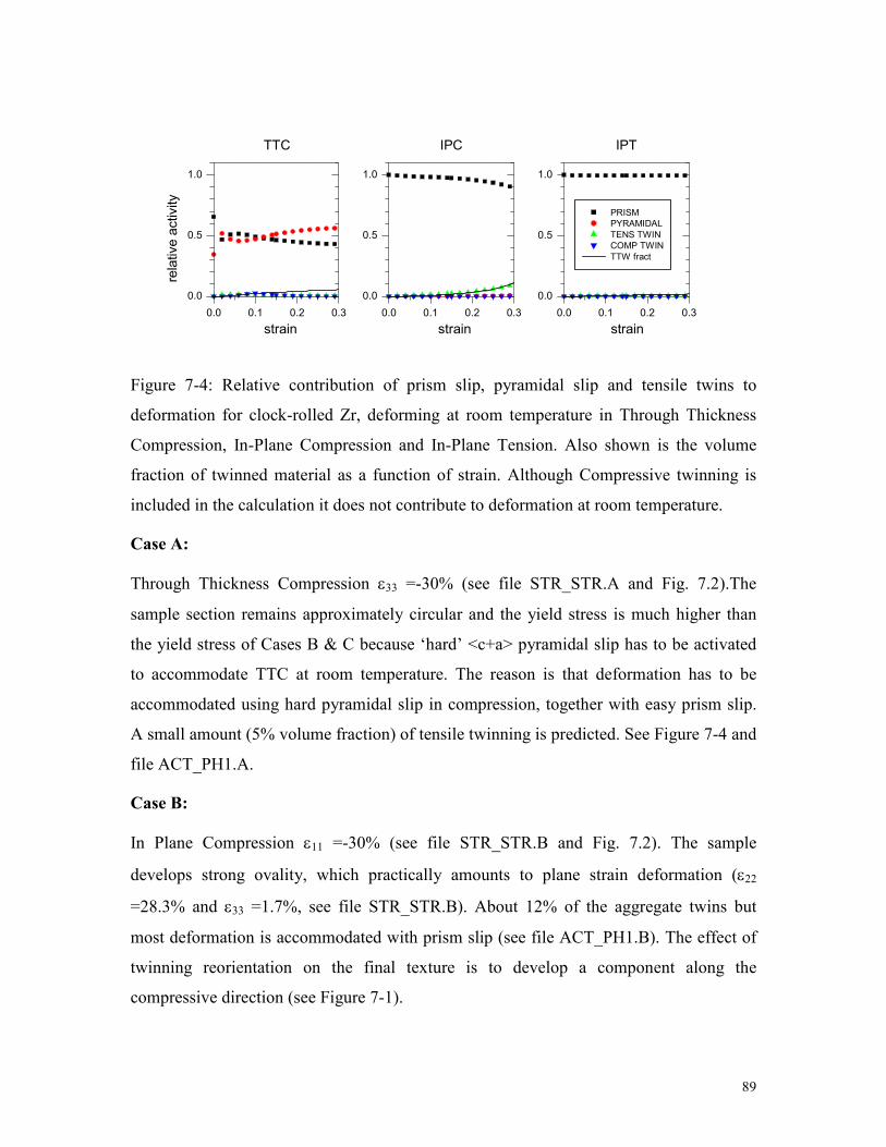
89

0.0 0.1 0.2 0.3

0.0

0.5

1.0

0.0 0.1 0.2 0.3

0.0

0.5

1.0

0.0 0.1 0.2 0.3

0.0

0.5

1.0

IPTIPCTTC

relative activity

PRISM

PYRAMIDAL

TENS TWIN

COMP TWIN

TTW fract

strain strain

strain

Figure 7-4: Relative contribution of prism slip, pyramidal slip and tensile twins to

deformation for clock-rolled Zr, deforming at room temperature in Through Thickness

Compression, In-Plane Compression and In-Plane Tension. Also shown is the volume

fraction of twinned material as a function of strain. Although Compressive twinning is

included in the calculation it does not contribute to deformation at room temperature.

Case A:

Through Thickness Compression ε33 =-30% (see file STR_STR.A and Fig. 7.2).The

sample section remains approximately circular and the yield stress is much higher than

the yield stress of Cases B & C because ‘hard’ <c+a> pyramidal slip has to be activated

to accommodate TTC at room temperature. The reason is that deformation has to be

accommodated using hard pyramidal slip in compression, together with easy prism slip.

A small amount (5% volume fraction) of tensile twinning is predicted. See Figure 7-4 and

file ACT_PH1.A.

Case B:

In Plane Compression ε11 =-30% (see file STR_STR.B and Fig. 7.2). The sample

develops strong ovality, which practically amounts to plane strain deformation (ε22

=28.3% and ε33 =1.7%, see file STR_STR.B). About 12% of the aggregate twins but

most deformation is accommodated with prism slip (see file ACT_PH1.B). The effect of

twinning reorientation on the final texture is to develop a component along the

compressive direction (see Figure 7-1).

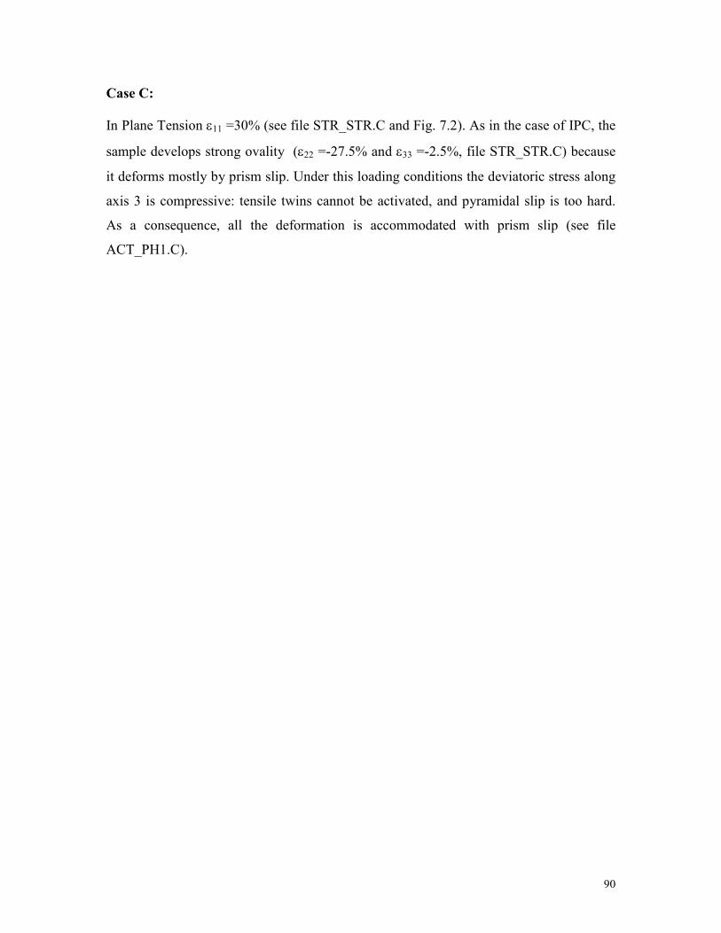
90

Case C:

In Plane Tension ε11 =30% (see file STR_STR.C and Fig. 7.2). As in the case of IPC, the

sample develops strong ovality (ε22 =-27.5% and ε33 =-2.5%, file STR_STR.C) because

it deforms mostly by prism slip. Under this loading conditions the deviatoric stress along

axis 3 is compressive: tensile twins cannot be activated, and pyramidal slip is too hard.

As a consequence, all the deformation is accommodated with prism slip (see file

ACT_PH1.C).

91

EXAMPLE 8: Compression of olivine (MgSiO4 )

Olivine (orthorhombic) enters in the composition of the Earth mantle. Olivine texture

affects the characteristics of seismic wave propagation.

For a comprehensive discussion of simulation and experiments see Kocks et al (2000; Ch.

6, Sec. 1.4; Ch. 7, Sec. 3.5 and Ch. 11, Sec. 5.4).

This example is meant to familiarize the user with an application of VPSC to a material

which lacks five independent slip systems, and show that the self-consistent formalism

can still be used for describing plastic deformation to such systems. It also shows how to

use the POSTMORTEM file, which is a feature of VPSC that allows to start from a

previous deformation state, or to provide an initial guess for the first deformation step.

Run conditions:

• Initial random texture (RAND500.TEX 500 orientations).

• Orthorhombic crystals with slip on:

(010)<100> : 4.00 =τ and no hardening

(001)<100> : 4.00 =τ and no hardening

(010)<001> : 4and0.1 10 =θ=τ linear hardening.

In order to close the yield surface the following auxiliary slip systems with high CRSS

are considered:

(110)<1-10>:0 15.0 and 4τ = θ = linear hardening.

(021)<1-12>:0 15.0 and 4τ = θ = linear hardening.

• Uniaxial compression. Strain increments of 2% up to ε33=50% at a rate of 1-s.

Case A:

Compression is simulated using the 5 slip modes described above. Texture and activity is

recorded for comparison with Case B. Particularly relevant is the output file

POSTMORT.OUT, containing the initial stress tensor in every grain, and the initial

polycrystal compliance. Observe that this file is written just after the first deformation

92

step (ISAVE=1) but the simulation is run up to 25 deformation steps. POSTMORT.OUT

can be written at any step in the deformation process, and used to restart the code from

the associated polycrystal state.

Deformation is accommodated mostly by the three soft modes, which contribute from 90

to 80% of the shear (see ACT_PH1.a). Specifically, the mode (021)<1-12> exhibits a

non-negligible activity in Case A, despite being much harder. The presence of the two

hard modes has the effect of increasing the stress and the average number of active

systems per grain by comparison with Case B (see Fig. 8.2). The final texture, though, is

not affected by the extra slip modes (see Fig. 8.1).

Case B:

Compression is simulated using the 3 slip modes which are actually observed in olivine.

The file POSTMORT.OUT of Case A is copied into POSTMORT.IN, and the variable

IRECOVER is set to 1 in VPSC7.IN. The Single Crystal Yield Surface is open, but the

run is started from the initial state contained in POSTMORT.IN in order to avoid the

initial Taylor guess which is the default in VPSC. The code converges and simulates

compression up to 50%. The final texture and the system activity are shown in Figure 8-1

and Figure 8-2. The final texture resembles the experimental one (Kocks et al, 2000) and

deformation is accommodated using less than 3 active systems per grain (see Figure 8-2).

See output files TEX_PH1.b and ACT_PH1.b. A comparison with Case A (files

TEX_PH1.a and ACT_PH1.a) shows that the final texture is similar.

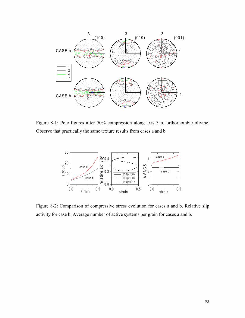
93

CASE b

CASE a

1

1

1

2

4

7

3 3 3 (100) (010) (001)

Figure 8-1: Pole figures after 50% compression along axis 3 of orthorhombic olivine.

Observe that practically the same texture results from cases a and b.

0.0 0.5

0.0

0.2

0.4

0.0 0.5

0

2

4

(010)<100>

(001)<100>

(010)<001>relative activity

stra in

case a

case b

AVACS

s train

0.0 0.5

0

10

20

30

case b

case a

s train

stress

Figure 8-2: Comparison of compressive stress evolution for cases a and b. Relative slip

activity for case b. Average number of active systems per grain for cases a and b.

94

EXAMPLE 9: Compression of polycrystaline ice (strain imposed and creep)

Due to the very large plastic anisotropy of hcp ice (i.e. while almost all the deformation

in the single crystals is carried by basal dislocations, basal slip provides only two

independent slip systems), the prediction of texture development of polycrystalline ice is

a challenging problem serving to discriminate among the various SC approaches.

Moreover, a better understanding of the deformation mechanisms and the microstructural

evolution of ice deforming in compression is relevant in glaciology, since compression

(together with shear) is one of the main deformation modes of glacier ice. In what

follows, we will use the basal texture factor along the axial direction (defined as the

weighted average of the projections of the c-axis along that direction) to characterize the

evolving texture of ice in compression.

Run conditions:

• Initial random texture (RAND500.TEX: 500 orientations).

• Hexagonal ice crystals deforming by easy (0001)<11-20> basal slip, hard (10-

10)<11-20> prismatic <a> slip ( bas20pr τ×=τ ), and harder (11-2-2)<11-23> pyramidal

<c+a> slip ( bas200pyr τ×=τ ). File ICE.SX.

Case A:

Uniaxial compression (strain fully imposed). 30 strain increments of 5%, up to ε=150%

at a rate of 1x10-8

(order of magnitude compatible with glacier ice deformation) (file

COMP150.3) using tangent (TG), affine (AF) and second-order linearization (SO). Files

extensions are TGD, AFD and SOD. The auxiliary program TFACTOR.FOR uses

TFACTOR.IN (=TEX_PH1.*) and gives the evolution on the basal texture factor along

the axial direction.

On the one hand, the ‘stiff’ Taylor and SC secant models are not suitable to simulate

plastic deformation of polycrystalline ice because the strong constraints that these models

impose upon strain are incompatible with the shortage of independent slip systems in ice.

On the other hand, the compression textures of ice typically exhibit a strong basal pole

maximum along the axial direction. The formation of this maximum is related with the

95

crystallographic plastic rotations associated with basal slip. However, as the basal poles

become aligned with the axial direction, the basal slip systems become unfavorably

oriented to accommodate deformation. Therefore, at large strains, even a ‘soft’ model

like the tangent SC fails in reproducing the observed texture, with only basal slip. Up to

now, the oversimplified Sachs model (which completely disregards strain compatibility)

has been the only approach able to give a reasonable effective behavior with predominant

basal slip at large strains, when the basal texture along the compressive direction

becomes very strong.

Fig. 9-1 shows the compression texture evolution (in terms of the basal texture factor

along the axial direction), the effective stress, the relative basal activity, and the average

number of active slip systems per grain, for the case of an initially random ice

polycrystal. As expected, all models predict an increase of the basal texture factor along

the axial direction, and a progressive geometric hardening. The tangent and the affine

models predict the fastest and the slowest alignment of basal poles along the compression

direction. This is consistent with the initial highest basal activity predicted by the tangent

model, followed by the ones obtained with the SO and the affine formulations. However,

at around 75% strain, the tangent results show a sudden drop in the basal activity,

together with an increase in the effective stress (not attributable to geometric hardening

only) and in the number of active deformation systems. All this indicates that, at large

compressive deformation, the strain accommodation starts requiring the activation of the

200 times harder pyramidal systems. In other words, under the tangent SC approach, the

basal slip by itself is not enough to accommodate the compressive deformation when the

basal poles become strongly aligned with the compression direction. The SO results are

superior to the affine results, since the deformation takes place at higher basal activities,

and also to the tangent results, since the SO model does not require the activation of the

hard pyramidal mode, even after the texture factor reaches the value at which the tangent

model predictions start to deteriorate.

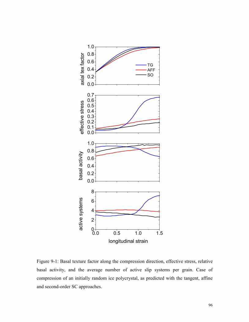
96

0.0

0.2

0.4

0.6

0.8

1.0

0.0

0.2

0.4

0.6

0.8

1.0

0.00.10.20.30.40.50.60.7

0.0 0.5 1.0 1.50

2

4

6

8

axial tex factor

TG

AFF

SO

basal activity

effective stress

longitudinal strain

active systems

Figure 9-1: Basal texture factor along the compression direction, effective stress, relative

basal activity, and the average number of active slip systems per grain. Case of

compression of an initially random ice polycrystal, as predicted with the tangent, affine

and second-order SC approaches.

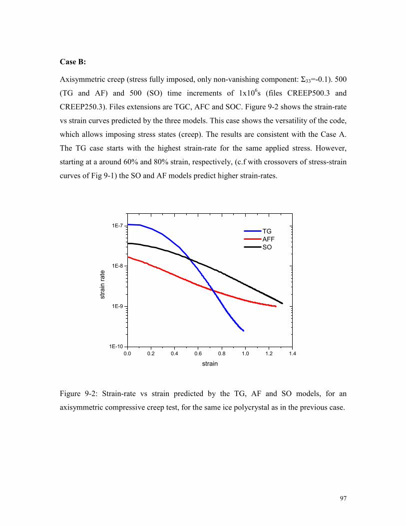
97

Case B:

Axisymmetric creep (stress fully imposed, only non-vanishing component: Σ33=-0.1). 500

(TG and AF) and 500 (SO) time increments of 1x106s (files CREEP500.3 and

CREEP250.3). Files extensions are TGC, AFC and SOC. Figure 9-2 shows the strain-rate

vs strain curves predicted by the three models. This case shows the versatility of the code,

which allows imposing stress states (creep). The results are consistent with the Case A.

The TG case starts with the highest strain-rate for the same applied stress. However,

starting at a around 60% and 80% strain, respectively, (c.f with crossovers of stress-strain

curves of Fig 9-1) the SO and AF models predict higher strain-rates.

0.0 0.2 0.4 0.6 0.8 1.0 1.2 1.4

1E-10

1E-9

1E-8

1E-7 TG

AFF

SO

strain rate

strain

Figure 9-2: Strain-rate vs strain predicted by the TG, AF and SO models, for an

axisymmetric compressive creep test, for the same ice polycrystal as in the previous case.

98

EXAMPLE 10: Equal Channel Angular Extrusion of FCC

This example is meant to familiarize the user with the simulation of sequential processes,

consisting of plastic forming and rigid rotations of the sample (described in Section

1.3.1). It also uses the option of ‘grain fragmentation’ described in Section 2.3.1. ECAE

consists in extruding the sample repeatedly through a 90° die. In each pass about 100%

shear strain is enforced with the advantage that the section of the sample is kept constant.

This process is meant to substantially reduce the grain size, while increasing yield stress

and retaining ductility. In practice, four extrusion routes are used, and each one imposes

a different deformation history to the sample. Here we describe two of them: Route BA

and Route C, and simulate two passes in each case. The extrusion process through the

die is the same for all routes and passes (process file ECAE.50), and for all routes the

sample is rotated 90°CW around die axis 3, in order to reinsert it in the die. What

differentiates the routes is an extra rotation around axis 2 of the die, before reinserting it.

Route A: no rotations.

Route BA: alternate rotations of 90°CW, 90°CCW, 90°CW, etc, around die axis 2.

Route BC: same rotations of 90°CW, 90°CW, 90°CW, etc, around die axis 2.

Route C: same rotations of 180°CW, 180°CW, 180°CW,etc, around die axis 2. This

route reverses the sense of shear at each pass.

For the simulations presented in Example 10 we use the following conditions:

• Initial random texture (file RAND500.TEX) with 500 orientations.

• FCC crystals with slip on (111)<110> and no hardening 0 1 0 1

1, 0, 0, 0τ = τ = θ = θ = (file

FCC.SX).

• Process file: 50 steps of shear at 45° with respect to the die axes (file ECAE.50),

which represents a shear of ε12=100%. The Exit:Entry:Flow axes of the die are axis

1:2:3 respectively

Case BA:

99

The input file is VPSC7.inB; the output files have extension *.Ba. An input file

POLE8.inB is provided for plotting the sequence of (111) poles for the initial, extruded,

rotated and extruded sample. A plot of the poles is in file POLES_Ba.pdf

Case C:

The input file is VPSC7.in; the output files have extension *.C

See below the sequence of (111) poles that result from each process applied to the sample

along both routes.

100

EXAMPLES of VPSC7FE last update April 2007!

The following describes in a summarily way some benchmark runs done with the

Material Subroutine version of VPSC7. The user is supposed to be familiar with VPSC7

first. Using SUBROUTINE VPSC7_FE as a material subroutine with an FE code will

require to understand I/O protocols and figure out the transfer and storage of arrays

specific to VPSC. The driver VPSC7FE contains comments that should be helpful in

doing so.

In what follows we explain cases #2 to #5. The distribution folders contain the input and

output files associated with these cases. Typically, output consists in stress-strain history

and final texture. In all cases we run three elements simultaneously, imposing a different

strain path to each.

Case 2a: Three FCC initially random aggregates with 500 grains are subjected to

%6033 =ε in compression, tension and rolling.

Case 2b: Same as before, except that the aggregates are subjected to %3033 =ε , a

POSTMORTEM file is created and an additional 30% is imposed starting from the

intermediate state. Case 2a and Case 2b give the same final result.

Case 3: This case tests the multi-phase capability. An aggregate containing 500 random

FCC grains and 300 random BCC grains. We assume 60% FCC volume fraction and 40%

BCC volume fraction. The FCC deforms by 111<110> slip, and the BCC by

110<111> and 112<111>. Compression, tension and rolling are imposed to 30%

strain.

Case 4: This case tests the twinning capability. Three elements containing a Zr aggregate

with an initial clock-rolled texture are deformed in Through Thickness Compression, In

Plane Compression and In Plane Tension up to 30%. We use the Zr hardening parameters

corresponding to 76K, where prism slip, tensile twins and compressive twins are active.

We verified that the result coincides with there separate and independent runs of VPSC7,

one for each deformation mode. We also controlled the POSTMORTEM capability by

running up to 15% and restating from such state.

101

Case 5: This cases tests the twinning capability in combination with the multi-phase

capability. The same aggregate as in Case 4 (representing 40% volume fraction) is mixed

with 60% volume fraction of FCC grains (500 of them). Through Thickness

Compression, In Plane Compression and In Plane Tension are applied up to 30%. The

final texture for the HCP and FCC phases are representative of the deformation mode

imposed.

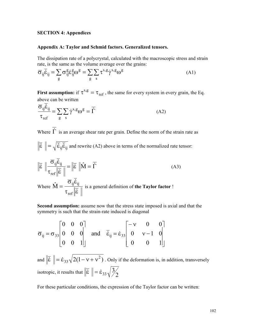
102

SECTION 4: Appendices

Appendix A: Taylor and Schmid factors. Generalized tensors.

The dissipation rate of a polycrystal, calculated with the macroscopic stress and strain

rate, is the same as the volume average over the grains:

∑∑∑ ωγτ=ωεσ=εσg

gg,s

s

g,s

g

ggij

gijijij ɺɺɺ (A1)

First assumption: if refg,s τ=τ , the same for every system in every grain, the Eq.

above can be written

Γ=ωγ=τ

εσ∑∑ ɺɺ

ɺ

g s

gg,s

ref

ijij (A2)

Where Γɺ is an average shear rate per grain. Define the norm of the strain rate as

ijijεε=ε ɺɺɺ and rewrite (A2) above in terms of the normalized rate tensor:

Γ=ε=ετ

εσε ɺɺ

ɺ

ɺɺ M

ref

ijij (A3)

Where ετ

εσ=

ɺ

ɺ

ref

ijijM is a general definition of the Taylor factor !

Second assumption: assume now that the stress state imposed is axial and that the

symmetry is such that the strain-rate induced is diagonal

−ν

ν−

ε=ε

σ=σ

100

010

00

and

100

000

000

33ij33ij ɺɺ

and )1(2 233 ν+ν−ε=ε ɺɺ . Only if the deformation is, in addition, transversely

isotropic, it results that 2

333ε=ε ɺɺ

For these particular conditions, the expression of the Taylor factor can be written:

103

23

23

M

ref

33

33ref

3333

ref

ijij

τ

σ=

ετ

εσ=

ετ

εσ=

ɺ

ɺ

ɺ

ɺ

Which can be written as: refref33 MM2

3 τ=τ=σ

Where M2

3M = is what is defined in the literature as the Taylor factor.

And the expression above for the rates can be rewritten as:

Γ=ε=ε=ε ɺɺɺɺ MM2

3M 3333

A generalized Schmid factor

The Schmid factor is a geometric factor defined for uniaxial stress states as the ratio

between the resolved shear in a slip plane n and along the slip direction b, over the

applied uniaxial stress. Two simple special cases, axial tension and simple shear, are

sketched below.

The corresponding stress tensors are

σ

σ

=σ

σ

=σ

000

00

00

and

000

000

00

12

12

ij

11

ij

The corresponding Schmid tensors are:

C1

C2

τr n _

b

_

ө

σ11

Axial tension

C1

C2

τr n _

b

_

σ12

Simple shear

104

1SandsincosS12

res

11

res =στ

=θθ=στ

=

If we define a general Schmid tensor as

σ

σ=

στ

= ijijresm

S

It reduces to the expressions above for the two simple cases, and can be applied to any

arbitrary stress tensor.

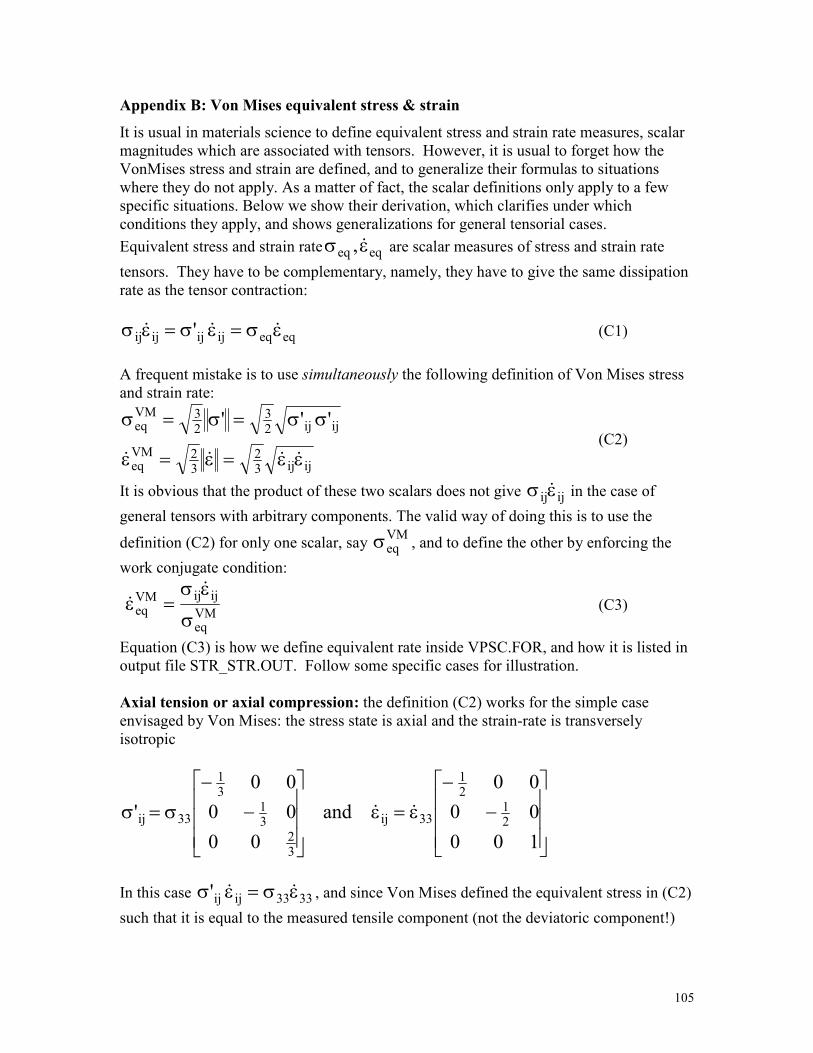
105

Appendix B: Von Mises equivalent stress & strain

It is usual in materials science to define equivalent stress and strain rate measures, scalar

magnitudes which are associated with tensors. However, it is usual to forget how the

VonMises stress and strain are defined, and to generalize their formulas to situations

where they do not apply. As a matter of fact, the scalar definitions only apply to a few

specific situations. Below we show their derivation, which clarifies under which

conditions they apply, and shows generalizations for general tensorial cases.

Equivalent stress and strain rate eqeq ,εσ ɺ are scalar measures of stress and strain rate

tensors. They have to be complementary, namely, they have to give the same dissipation

rate as the tensor contraction:

eqeqijijijij ' εσ=εσ=εσ ɺɺɺ (C1)

A frequent mistake is to use simultaneously the following definition of Von Mises stress

and strain rate:

ijij32

32VM

eq

ijij2

3

2

3VMeq '''

εε=ε=ε

σσ=σ=σ

ɺɺɺɺ

(C2)

It is obvious that the product of these two scalars does not give ijijεσ ɺ in the case of

general tensors with arbitrary components. The valid way of doing this is to use the

definition (C2) for only one scalar, say VMeqσ , and to define the other by enforcing the

work conjugate condition:

VMeq

ijijVMeq

σ

εσ=εɺ

ɺ (C3)

Equation (C3) is how we define equivalent rate inside VPSC.FOR, and how it is listed in

output file STR_STR.OUT. Follow some specific cases for illustration.

Axial tension or axial compression: the definition (C2) works for the simple case

envisaged by Von Mises: the stress state is axial and the strain-rate is transversely

isotropic

−

−

ε=ε

−

−

σ=σ

100

00

00

and

00

00

00

'21

21

33ij

32

31

31

33ij ɺɺ

In this case 3333ijij' εσ=εσ ɺɺ , and since Von Mises defined the equivalent stress in (C2)

such that it is equal to the measured tensile component (not the deviatoric component!)

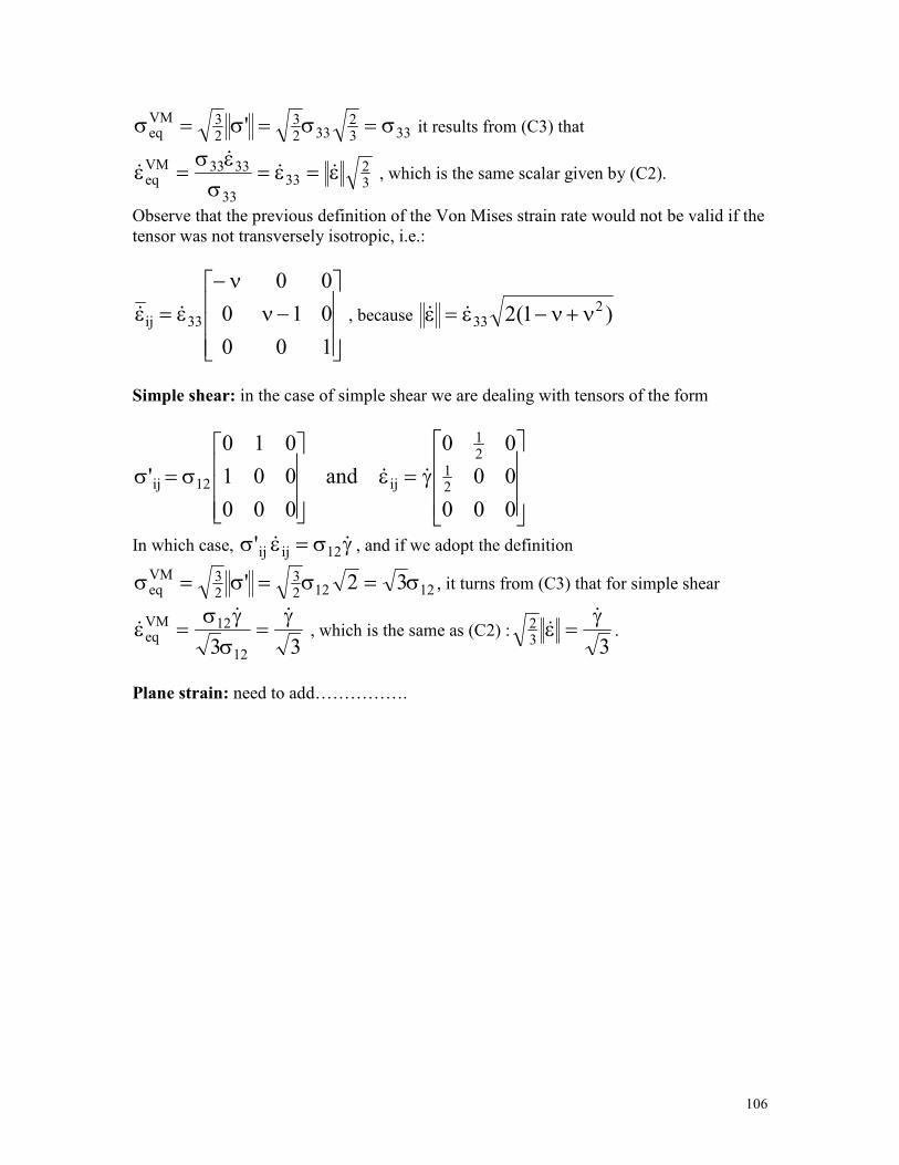
106

3332

3323

23VM

eq ' σ=σ=σ=σ it results from (C3) that

32

33

33

3333VMeq ε=ε=

σεσ

=ε ɺɺɺ

ɺ , which is the same scalar given by (C2).

Observe that the previous definition of the Von Mises strain rate would not be valid if the

tensor was not transversely isotropic, i.e.:

−ν

ν−

ε=ε

100

010

00

33ij ɺɺ , because )1(2 233 ν+ν−ε=ε ɺɺ

Simple shear: in the case of simple shear we are dealing with tensors of the form

γ=ε

σ=σ

000

00

00

and

000

001

010

'21

21

ij12ij ɺɺ

In which case, γσ=εσ ɺɺ 12ijij' , and if we adopt the definition

121223

23VM

eq 32' σ=σ=σ=σ , it turns from (C3) that for simple shear

33 12

12VMeq

γ=

σγσ

=εɺɺ

ɺ , which is the same as (C2) :33

2 γ=εɺ

ɺ .

Plane strain: need to add…………….

107

Appendix C: Voce hardening and VPSC algorithm

Express Kocks-Mecking equation for evolution of density in terms of total shear rate in

grain and Taylor law for the threshold stress sτ (see Karaman et al, 2000):

( )Γρ−ρ=ρ ɺɺ 21kk (C1)

ραµ+τ=τ b0 (C2)

Here s

s

Γ = γ∑ɺ ɺ is the sum of the shear rates over all systems. From (C2):

b/)( 0 αµτ−τ=ρ (C3)

and ρρ

αµ=τ ɺɺ

2

b (C4)

Replace (C3) in (C1), and replace (C1) in (C4):

( )Γτ−=Γ

τ

τ

θ−τ+τ

τ

θ=Γ

τ−τ−αµ

=τ ɺɺɺɺ ba)()(k2

bk

1

010

1

0021 (C5)

Where we define: 1

010

1

02

1

010 b,)(a,

2

k,

2

bk

τθ

=τ+ττθ

==τθαµ

=θ (C6)

Integrating (C5) gives:

Γτ

τ Γ=τ−−

00)baln(

b

1

From where: Γ−τ−=τ− b0 e)ba()ba(

Replacing the parameters defined in (C6) leads to a saturating Voce law describing the

evolution of the threshold with shear:

))exp(1(1

010 τ

θΓ−−τ+τ=τ (C7)

The increase in the threshold stress of a system due to shear activity 'sγ∆ in the grain

systems is calculated as:

∑ γ∆Γτ

=τ∆'s

's'sss

s hd

ˆd (C8)

where

108

τθ

Γ−Γθτθ

+τθ

Γ−θ−ττθ

+θ=Γτ

)exp()exp()(d

ˆd

1

01

1

0

1

011

1

01

s (C9)

The threshold associated with each system in each grain is updated inside SUBROUTINE

UPDATE_CRSS_VOCE. However, the incremental expression (C8) represents a forward

extrapolation which tends to overestimate the hardening and make it dependent on the

step size, more so when the derivative is large. As a consequence, we have implemented

an analytic integration of Eq. (C9) inside SUBROUTINE UPDATE_CRSS_VOCE. The

procedure is as follows.

∫ ∑∆Γ+Γ

Γ

γΓτ

=τ∆0

0's

's'sss

s dhd

ˆd (C10)

If we express: )10(and0

ss0

s <α<∆Γα+Γ=Γγ∆α+γ=γ

Then: Γ∆Γγ∆

=αγ∆=γα∆Γ=Γ dddanddds

ss

Replacing in (C10):

∫ ∑∫ ∑∆Γ+Γ

Γ

=α

=α

∆Γγ∆

ΓΓτ

=Γ∆Γγ∆

Γτ

=τ∆0

0's

s'ss

s1

0 's

s'ss

ss hd

d

ˆddh

d

ˆd (C11)

Replacing in (C11) the derivative given by (C9), recalling the primitive integrals

1

0

2

axaxaxax awhere)ax1(

a

edxxeande

a

1dxe

τ

θ=+−=−=

−−−− ∫∫

and accounting for the integration extremes, gives the incremental change of the

threshold stress as:

Γ+−∆Γ+Γ+θ

−

−θ−τ

−∆Γθ

∆Γγ∆

=τ∆∆Γ−Γ−

∆Γ−Γ−

∑]a1[)](a1[ee

a

)1e(ea

a

h

00aa1

aa111

's

s'sss

0

0

(C12)

109

Appendix D: Crystal rotation and misorientation

Equation (3-1) describes the rate of change of the crystal orientation matrix as

c c c c,R

oR R where (W W )= Ω Ω = −ɺ ɺ ɺ (D1)

If the tensor Ωɺ is assumed to be constant within a time increment, the solution to (D1) is

c c cR (t t) R (t) exp( t) R (t) exp( )+ ∆ = Ω∆ = Ωɺ (D2)

Where tΩ = Ω∆ɺ is a skew symmetric tensor and can be written in a form that will give

a straightforward meaning to its components, namely

3 2

3 1

2 1

0

ˆ0

0

−ω ω Ω = ω −ω = ωΩ −ω ω

where (D3)

3 2

2 2 2

3 1 1 2 3

2 1

ˆ ˆ0

ˆ ˆ ˆ0 and

ˆ ˆ 0

−ω ω Ω = ω −ω ω = ω +ω +ω −ω ω

According to (D2), updating the crystal orientation matrix requires to evaluate the

exponential of a tensor, which is done using the Taylor expansion n

n 0

exp( )n!

∞

=

ΩΩ = ∑ (D4)

But because of the special form (D3) of Ω , the powers have the property: 0

1

2 2 2 2

3 3

4 4 2

5 5

I

ˆ

ˆ ˆ ˆ( I )

ˆ

ˆ

ˆ

.......

Ω =

Ω = ωΩ

Ω = ω Ω = ω − +ω⊗ω

Ω = −ω Ω

Ω = −ω Ω

Ω = ω Ω

(D5)

Replacing in (D4) and regrouping alternate terms, one obtains a series expansion for sinω

and cosω

110

2 22 3 4

3 5 2 4 62

2

ˆ ˆ ˆ ˆexp( ) I ...

1! 2! 3! 4!

ˆ ˆexp( ) I ... ...1! 3! 5! 2! 4! 6!

ˆ ˆexp( ) I sin (1 cos )

Ω Ω Ω ΩΩ = +ω +ω −ω −ω

ω ω ω ω ω ωΩ = +Ω − + − +Ω − + −

Ω = +Ω ω+ Ω − ω

(D6)

This form of the transformation matrix based on a spin ω around a normalized axis ω is

often referred to as the Rodrigues equation. It is also relevant to the definition of

misorientation between two crystal systems. If one assumes that RA and RB transform

from crystals A and B to sample axes, then RBT RA transforms from crystal A to crystal

B. If one expresses such transformation using Rodrigues it will be of the form

T 2

B Aˆ ˆR R I sin (1 cos )= +Ω ω+Ω − ω (D7)

Taking the trace of the tensors and using the form of Ω and 2Ω given by (D3) and (D5)

one obtains the rotation angle (misorientation angle) that makes A and B coincide

T

1 B Atr(R R ) 1

cos2

− −ω =

(D8)