VT EPSCoR Research on Adaptation to Climate Change (RACC)

Internship Program - Summer 2015

VT EPSCoR Center for Workforce Development and Diversity Saint Michael’s College Email: cwdd@smcvt.edu One Winooski Park, Box 137 Website: www.uvm.edu/~cwdd Colchester, VT 05439 Fax: 802.654.2940 Office: 251 Founder’s Annex, Saint Michael’s College Lab: 126 Cheray Science Hall, Saint Michael’s College, Lab Phone: 802.654.1916 Laura Yayac, Project Manager Janel Roberge, Research Technician Phone: 802.654.3270 Phone: 802.654.3271 Email: lyayac@smcvt.edu Email: jroberge@smcvt.edu

Lindsay Wieland, Director Phone: 802.654.3272 Email: lwieland@smcvt.edu

Manual Contents

Section 1: Payroll Instructions

Section 2: Research

Section 3: Field Safety

Section 4: Background

VT EPSCOR

RACC Intern Payroll Instructions and Schedule

June 1 – August 7, 2015

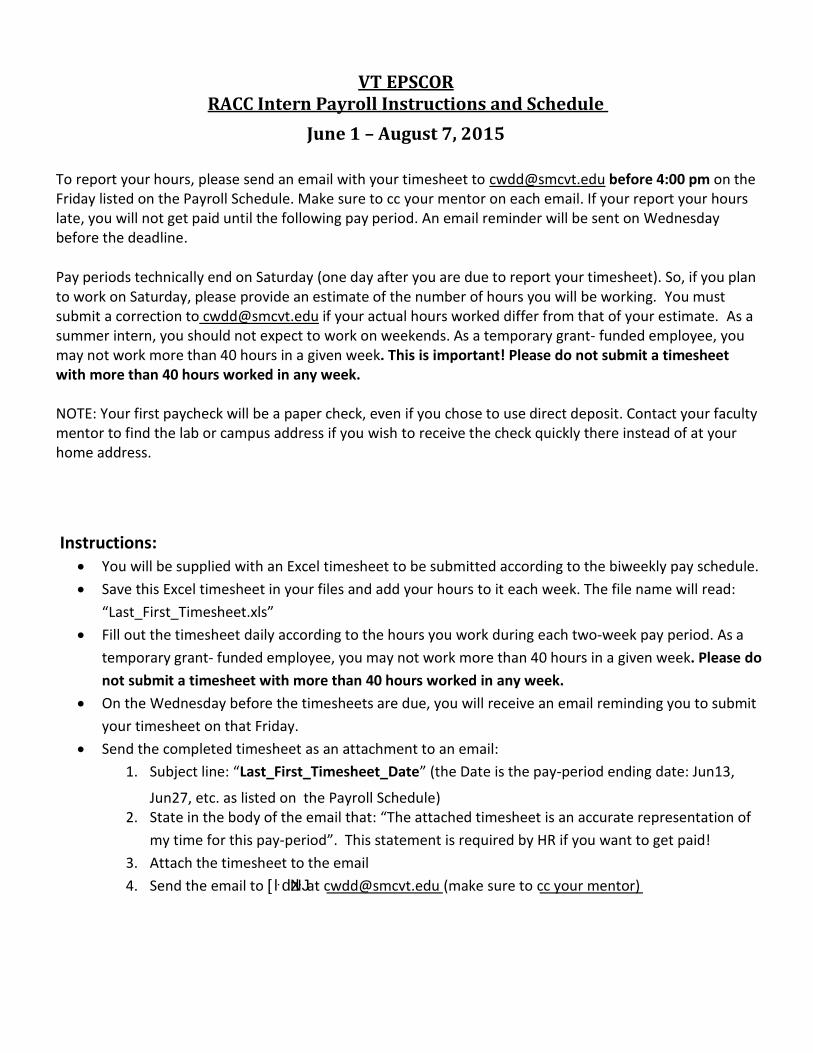
To report your hours, please send an email with your timesheet to cwdd@smcvt.edu before 4:00 pm on the Friday listed on the Payroll Schedule. Make sure to cc your mentor on each email. If your report your hours late, you will not get paid until the following pay period. An email reminder will be sent on Wednesday before the deadline. Pay periods technically end on Saturday (one day after you are due to report your timesheet). So, if you plan to work on Saturday, please provide an estimate of the number of hours you will be working. You must submit a correction to cwdd@smcvt.edu if your actual hours worked differ from that of your estimate. As a summer intern, you should not expect to work on weekends. As a temporary grant- funded employee, you may not work more than 40 hours in a given week. This is important! Please do not submit a timesheet with more than 40 hours worked in any week. NOTE: Your first paycheck will be a paper check, even if you chose to use direct deposit. Contact your faculty mentor to find the lab or campus address if you wish to receive the check quickly there instead of at your home address.

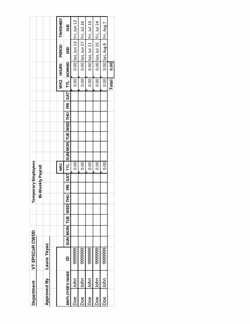
Instructions: You will be supplied with an Excel timesheet to be submitted according to the biweekly pay schedule.

Save this Excel timesheet in your files and add your hours to it each week. The file name will read:

“Last_First_Timesheet.xls”

Fill out the timesheet daily according to the hours you work during each two-week pay period. As a

temporary grant- funded employee, you may not work more than 40 hours in a given week. Please do

not submit a timesheet with more than 40 hours worked in any week.

On the Wednesday before the timesheets are due, you will receive an email reminding you to submit

your timesheet on that Friday.

Send the completed timesheet as an attachment to an email:

1. Subject line: “Last_First_Timesheet_Date” (the Date is the pay-period ending date: Jun13,

Jun27, etc. as listed on the Payroll Schedule) 2. State in the body of the email that: “The attached timesheet is an accurate representation of

my time for this pay-period”. This statement is required by HR if you want to get paid!

3. Attach the timesheet to the email

4. Send the email to [ŀdzNJŀ at cwdd@smcvt.edu (make sure to cc your mentor)

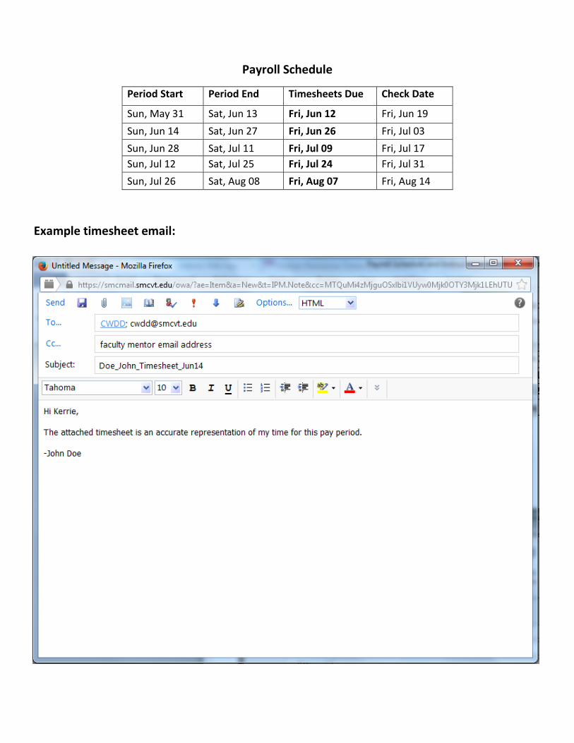
Payroll Schedule

Period Start Period End Timesheets Due Check Date

Sun, May 31 Sat, Jun 13 Fri, Jun 12 Fri, Jun 19

Sun, Jun 14 Sat, Jun 27 Fri, Jun 26 Fri, Jul 03

Sun, Jun 28 Sat, Jul 11 Fri, Jul 09 Fri, Jul 17

Sun, Jul 12 Sat, Jul 25 Fri, Jul 24 Fri, Jul 31

Sun, Jul 26 Sat, Aug 08 Fri, Aug 07 Fri, Aug 14

Example timesheet email:

De

pa

rtm

en

tV

T E

PS

Co

R C

WD

DT

em

po

rary

Em

plo

ye

es

B

i-W

ee

kly

Pa

yro

ll

Ap

pro

ve

d B

yL

au

ra Y

aya

c

WK

1W

K2

HO

UR

SP

ER

IOD

T

IMES

HEET

SU

NM

ON

TU

EW

ED

TH

UFR

IS

AT

TT

LS

UN

MO

NT

UE

WE

DT

HU

FR

IS

AT

TT

LW

OR

KED

EN

DD

UE

Doe

John

9999

999

0.0

00

.00

0.0

0Sa

t, J

un

13

Fri,

Ju

n 1

2

Doe

John

9999

999

0.0

00

.00

0.0

0Sa

t, J

un

27

Fri,

Ju

l 2

6

Doe

John

9999

999

0.0

00

.00

0.0

0Sa

t, J

ul

11

Fri,

Ju

l 1

0

Doe

John

9999

999

0.0

00

.00

0.0

0Sa

t, J

ul

25

Fri,

Ju

l 2

4

Doe

John

9999

999

0.0

00

.00

0.0

0Sa

t, A

ug

8Fr

i, A

ug

7

To

tal

0.0

0

EM

PL

OY

EE'S

NA

ME

ID

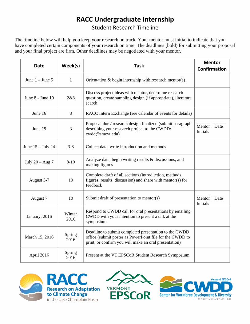
RACC Undergraduate Internship Student Research Timeline 

The timeline below will help you keep your research on track. Your mentor must initial to indicate that you have completed certain components of your research on time. The deadlines (bold) for submitting your proposal and your final project are firm. Other deadlines may be negotiated with your mentor.

Date  Week(s)  Task Mentor 

Confirmation 

June 1 – June 5 1 Orientation & begin internship with research mentor(s)

June 8 - June 19 2&3 Discuss project ideas with mentor, determine research question, create sampling design (if appropriate), literature search

June 16 3 RACC Intern Exchange (see calendar of events for details)

June 19 3 Proposal due / research design finalized (submit paragraph describing your research project to the CWDD: cwdd@smcvt.edu)

______ ______ Mentor Date Initials

June 15 – July 24 3-8 Collect data, write introduction and methods

July 20 – Aug 7 8-10 Analyze data, begin writing results & discussions, and making figures

August 3-7 10 Complete draft of all sections (introduction, methods, figures, results, discussion) and share with mentor(s) for feedback

August 7 10 Submit draft of presentation to mentor(s) _____ ______ Mentor Date Initials

January, 2016 Winter 2016

Respond to CWDD call for oral presentations by emailing CWDD with your intention to present a talk at the symposium

March 15, 2016 Spring 2016

Deadline to submit completed presentation to the CWDD office (submit poster as PowerPoint file for the CWDD to print, or confirm you will make an oral presentation)

April 2016 Spring 2016 Present at the VT EPSCoR Student Research Symposium

Data Analysis

You should begin thinking about your preparing your poster or presentation for the annual VT EPSCoR Student Research Symposium in April as soon as possible. Your poster or presentation will describe your research and your contribution to the overall RACC effort.

If your project includes data analysis, the CWDD data analysis tutorial may be useful. This tutorial guides you through the process of exploring and asking more in-depth analysis questions about your dataset. The tutorial can be found on the Vermont EPSCoR website here:

http://www.uvm.edu/~epscor/new02/?q=node/1027

The first link on the page that says “Complete Tutorial Series - All Modules” will open a pdf with all of the modules compiled into one document. The subsequent links are for accessing modules individually. The tutorial guides you through working with the online Streams Project dataset, which may or may not pertain to your work, however the guidance on working with datasets is applicable to many types of datasets. The following is a list of the individual modules and what they cover:

Module 1: What is science? Module 2: Understanding Streams Project Data Module 3: Refining and Retrieving Data Module 4: Data Exploration Module 5: Statistical Analysis Module 6: Summarizing Results and Drawing Conclusions

In this tutorial, statistical analysis is demonstrated using Microsoft Excel. Within each module, look for the “WATCH VIDEO” icon that looks like this:

These videos help you visualize a number of procedures outlined in the tutorial.

Presenting Your Data: VT EPSCoR Student Research Symposium

All participants of the RACC Undergraduate Internship program commit to presenting their research findings at the annual Vermont EPSCoR Student Research Symposium. A symposium is a great way for researchers to present and discuss their work and it provides an important channel for the exchange of information between researchers. At the Vermont EPSCoR Student Research Symposium, participants have the option to choose whether they present their research through a poster or an oral presentation. Both are great ways to share your work!

Posters versus Oral Presentations

Although it can be challenging to present a year’s worth of work in 10 minutes, oral presentations can be a rewarding experience because you are the only one front of an audience whose attention you know you have. Oral presentations are brief and consequently the presentation must be clearly and succinctly presented.

Posters are a visual presentation of information that is understandable to the viewer without verbal explanation. Poster presenters have the opportunity to share their work with one person at a time, over an extended period of time. This allows the presenter to describe and discuss their research in greater detail than would be possible in an oral presentation to significantly more people, and allows for dialogue with poster viewers.

Posters A research or academic poster provides a means of communicating your research at a conference or research symposium. Posters printed by Vermont EPSCoR are 3’ x 4’ (or 36’’ x 48”), horizontally or vertically aligned. Upload your final poster file when registering for the symposium by the deadline announced in early March. The CWDD will print and set up your poster at the symposium.

How to Create a Poster Using PowerPoint For many, this is the first time creating a research poster. Here are some tips for making an informative and attractive research poster:

1. Open PowerPoint 2. Click the ‘Design’ menu/tab at the top of the screen and select ‘Page Setup’

i. Change the dimensions of the slide from the default setting to: Width=48, Height=36 (for a horizontal poster), or Width=36, Height=48 (for a vertical poster). This is an important FIRST step – if you change the dimensions after putting content on the slide, you will have to re-format all text boxes, graphs, tables, photos, etc.

3. Critical poster elements: i. Title, Author(s) and affiliation(s)

ii. Abstract/Summary (optional) iii. Introduction/Background: a brief but important overview to secure the viewer’s attention iv. Materials and Methods: a brief description of the processes and procedures used, photos

(optional) should be >300dpi v. Results: outcomes, findings and data displayed through text, tables, graphs, photos, etc.

• Bulleted lists (rather than paragraphs) may help the reader understand the most important findings

• Tables, graphs and photos should have captions. Graphs should have a legend, avoid 3-D graphs as they are hard to interpret

vi. Discussion/Conclusions: summary or discussion of the significance and relevance of the results, identify possible future research

vii. References viii. Acknowledgements

ix. Please include the following text somewhere on the poster: Funding provided by NSF Grant EPS-1101317

4. Upload final poster file when registering for the symposium

Tips:

A. Use the “Designing Conference Posters” website to get ideas on poster layout and to download poster templates: http://colinpurrington.com/tips/academic/posterdesign

B. Choose a background and text color scheme. No need to go crazy: a white/light poster with black/dark text is often much easier to read than a multi-colored poster. Use cool/muted colors, solid colors, a color gradient, etc.

C. Lettering can make a difference in how easy-to-read your poster is. Here are some suggestions: • Title: at least 72 pt., bold preferred • Section Headings: at least 48 pt., bold preferred • Body Text: at least 24 pt.

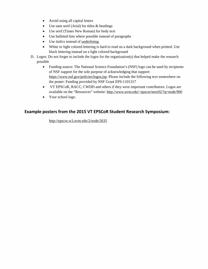
• Avoid using all capital letters • Use sans serif (Arial) for titles & headings • Use serif (Times New Roman) for body text • Use bulleted lists where possible instead of paragraphs • Use italics instead of underlining • White or light colored lettering is hard to read on a dark background when printed. Use

black lettering instead on a light colored background D. Logos: Do not forget to include the logos for the organization(s) that helped make the research

possible • Funding source: The National Science Foundation’s (NSF) logo can be used by recipients

of NSF support for the sole purpose of acknowledging that support: https://www.nsf.gov/policies/logos.jsp. Please include the following text somewhere on the poster: Funding provided by NSF Grant EPS-1101317

• VT EPSCoR, RACC, CWDD and others if they were important contributors. Logos are available on the “Resources” website: http://www.uvm.edu/~epscor/new02/?q=node/900

• Your school logo.

Example posters from the 2015 VT EPSCoR Student Research Symposium:

http://epscor.w3.uvm.edu/2/node/2635

Oral Presentations A research talk provides a means of communicating your research at a conference or research symposium. Oral presentations at the VT EPSCoR Student Research Symposium are limited to 10 minutes: 8 minutes to present your research, 2 minutes for the audience to ask questions. Presenters often use the general rule of “2 slides per minute”; however the number of slides needed varies based on the complexity of the content of the slides. Upload your final PowerPoint file when registering for the symposium by the deadline announced in early March or bring the file to the symposium on a USB drive. The CWDD will provide the computer, screen, podium, microphone and laser pointer for your use.

Oral Presentation Structure (suggested): • Title, Author(s), Affiliation (1 slide) • Outline, optional (1 slide): overview of the structure of your talk, some speakers prefer to put this

at the bottom of their title slide, audiences like predictability • Introduction/Background

o Motivation and problem statement (1-2 slides): Why should anyone care? Most researchers overestimate how much the audience knows about the problem they are addressing.

o Related Work (0-1 slides) o Methods (1 slide): Cover quickly in short talks

• Results (4-6 slides): Present key results and key insights. This is the main body of the talk. Its structure varies greatly as a function of the research conducted. Do not superficially cover all results; cover key result well. Do not just present numbers; interpret them to give insights. Do not put up large tables of numbers as your audience will not have time to take in that much information at once.

• Discussion/Conclusions (1 slide): summary or discussion of the significance and relevance of the results, identify possible future research.

• References • Acknowledgements • Please include the following text somewhere on your slides: Funding provided by NSF Grant

EPS-1101317 Logos: Do not forget to include the logos for the organization(s) that helped make the research possible!

• Funding source: The National Science Foundation’s (NSF) logo can be used by recipients of NSF support for the sole purpose of acknowledging that support: https://www.nsf.gov/policies/logos.jsp. Please include the following text somewhere on your slides: Funding provided by NSF Grant EPS-1101317

• VT EPSCoR, RACC, CWDD and others if they were important contributors. Logos are available on the “Resources” website: http://www.uvm.edu/~epscor/new02/?q=node/900

• Your school logo.

Example presentations from the 2015 VT EPSCoR Student Research Symposium: http://epscor.w3.uvm.edu/2/node/2634

Resources

Symposium Resources: http://www.uvm.edu/~epscor/new02/?q=node/1221

• Includes links to datasets available online, including:

Data and Data Analysis

• VT Department of Environmental Conservation Lake Champlain Long Term Monitoring • VT Department of Environmental Conservation Volunteer Monitoring • USGS Stream Gauge Data • Vermont Water Quality Data • NOAA Quality Controlled Local Climatological Data • VT EPSCoR Data Analysis Tutorials • Data Analysis in Excel

• Helpful hints on posters and oral presentations

• High resolution logos to include on your poster, etc.

Present your Research!

There are many venues in which you can participate and present the research you conduct this summer. You are required to present your project at the VT EPSCoR Student Research Symposium in the spring of 2016, and we encourage you to also present your research at other conferences to gain valuable experience. Scientific and policy associations and organizations exist for every discipline and most encourage undergraduate participation. Check with your department/college and faculty mentors to learn about these opportunities!

These are some annual symposia/conferences:

Vermont EPSCoR Student Research Symposium (Spring, annually) This symposium provides an opportunity for students, faculty, and other RACC researchers and interested groups to share their findings and learn about the status of the Research on Adaptation to Climate Change effort. (http://www.uvm.edu/~epscor/new02/?q=node/190) Lake Champlain Research Consortium - Spring Student Symposium (Late April, annually) The mission of the Lake Champlain Research Consortium is to coordinate and facilitate research and scholarship of the Lake Champlain ecosystem and related issues; to provide opportunities for training and education of students on lake issues; and to aid in the dissemination of information gathered through lake endeavors. (http://academics.smcvt.edu/lcrc/) Saint Michael’s College Symposium (Late April, annually) Sponsored by the SMC Undergraduate Research Committee, the Symposium is a day set aside by the College community for the presentation of student scholarship such as a thesis, research project, or performance. (http://academics.smcvt.edu/smcsymposium/Home.html) UVM Student Research Conference (Late April, annually) As part of the University of Vermont's weeklong celebration of student achievement, the UVM Student Research Conference (SRC) showcases the research and scholarly activity of undergraduate, graduate and medical students across campus. All students working on a research or creative project with a UVM faculty member are eligible to present some aspect of their research at this forum. Research and creative projects at any stage of completion are welcome. The event also serves as a resource for students who are not yet involved with research but wish to learn about how to engage in research pursuits. (http://www.uvm.edu/~uvmsrc/?Page=about/default.php&SM=about/_aboutmenu.html) Johnson State College Extended Classroom Experiences Showcase Event (April, annually) Faculty, staff, students, trustees, community partners and friends are invited to join us in a celebration and exhibition of student work outside of the classroom. (http://www.jsc.edu/Academics/BeyondTheClassroom/ECE.aspx) SACNAS Conference (Society for Advancement of Hispanics/Chicanos and Native Americans) in Science; October 29 - 31, 2015 In 2015, this national conference will be held in Maryland (8 miles south of Washington, D.C.). The SACNAS National Conference showcases cutting-edge science and features mentoring and training sessions for students and scientists at all levels. (http://sacnas.org/) Should you present at any of these symposia or others, please let CWDD know! Email us at cwdd@smcvt.edu with any updates on your professional presentation portfolio (say that three times fast ).

Research Internship Guidelines

As with any academic work, we expect the work that you do for the Vermont EPSCoR program to be completed in a professional manner using your own words and concepts, or proper citations where appropriate. Below are definitions and resources to assist you in conducting high quality, professional research.

Plagiarism Plagiarism is often thought of as passing work completed by someone else off as your own. This represents an extreme case. Plagiarism takes a number of subtler forms as well, from improper paraphrasing or citation of a resource, to passing an existing idea or concept off as your own. As you conduct your research and draft your poster or presentation, please review the following web page to familiarize yourself with the different forms of plagiarism:

http://www.plagiarism.org/

Plagiarism is a very serious offense and will not be tolerated by Vermont EPSCoR and the Research on Adaptation to Climate Change program.

Professionalism The Vermont EPSCoR staff, faculty, postdocs, and graduate students are all excited to be working with you, though it’s important to keep in mind that people have other time commitments. To best use your time and that of others, please consider the following:

Come to meetings prepared with ideas and questions you’d like to discuss.

If you need help or have questions related to your research don’t wait until the last minute to set up a meeting with your mentor.

Review your poster thoroughly yourself before submitting it to your mentor to review.

Do not wait until the last minute to have your poster reviewed.

Be on time – this applies to meetings, work, and deadlines.

Section 3: Field Safety

First Aid Kit When working in the field, it is important to be prepared for emergencies. Although you will not be traveling far from the vehicle when you visit field sites for the VT EPSCoR Project, accidents may still happen. Therefore, a well-stocked first aid kit is an important thing to have. Carry a first aid kit with you to your site or keep one in the vehicle. You may purchase a pre-made kit at the store, or you may make your own using the recommended list of items below as a reference. Whichever you chose, it is important to include any personal items such as medications and emergency phone numbers. Check the kit regularly and replace any used or out-of-date items. Adhesive bandages (assorted sizes) Antibiotic ointment Antiseptic wipes Instant cold compress Hydrocortisone ointment Scissors Sterile gauze pads (assorted sizes) Butterfly bandages Tweezers Prescription medications (asthma inhalers, Epipen) Emergency phone numbers Charged cell phone Always notify your mentor when you are going out into the field, and tell him/her where you will be and for how long you will be gone. Never go to a field site alone – always go with a partner.

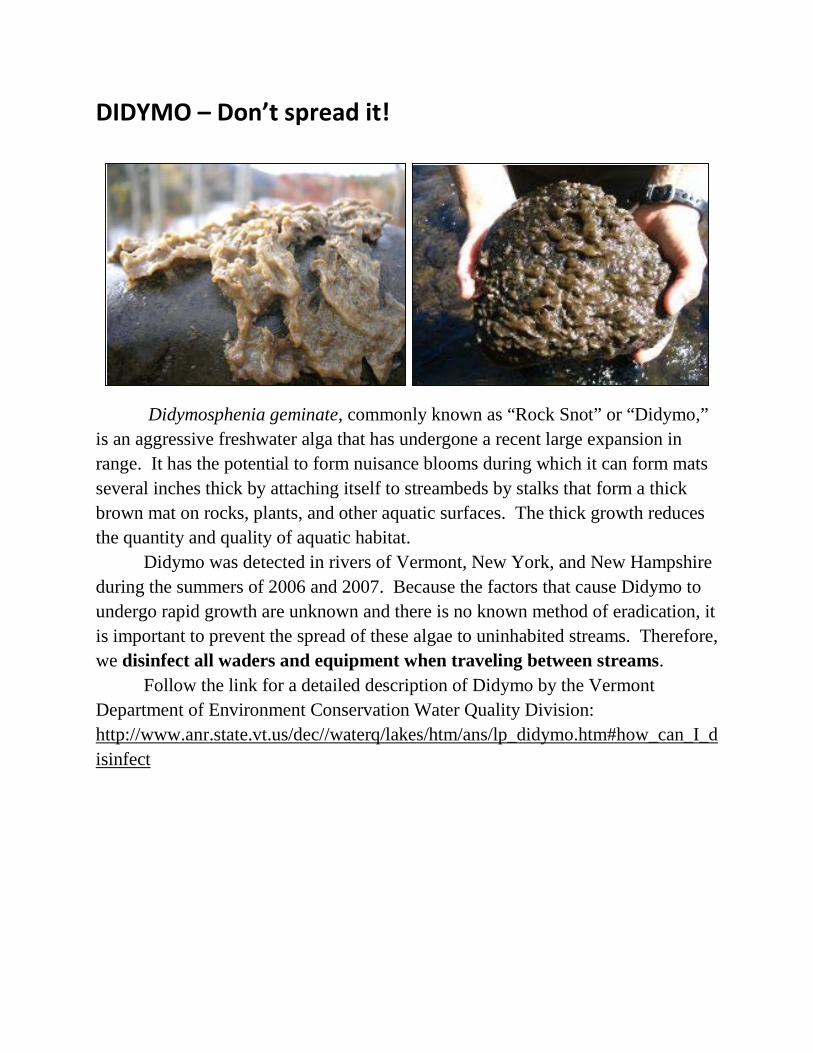
DIDYMO – Don’t spread it!

Didymosphenia geminate, commonly known as “Rock Snot” or “Didymo,” is an aggressive freshwater alga that has undergone a recent large expansion in range. It has the potential to form nuisance blooms during which it can form mats several inches thick by attaching itself to streambeds by stalks that form a thick brown mat on rocks, plants, and other aquatic surfaces. The thick growth reduces the quantity and quality of aquatic habitat.

Didymo was detected in rivers of Vermont, New York, and New Hampshire during the summers of 2006 and 2007. Because the factors that cause Didymo to undergo rapid growth are unknown and there is no known method of eradication, it is important to prevent the spread of these algae to uninhabited streams. Therefore, we disinfect all waders and equipment when traveling between streams.

Follow the link for a detailed description of Didymo by the Vermont Department of Environment Conservation Water Quality Division: http://www.anr.state.vt.us/dec//waterq/lakes/htm/ans/lp_didymo.htm#how_can_I_disinfect

Disinfecting Waders

If you will be walking around in streams, you will need to use concentrated Quaternary Ammonium Disinfectant (Quat solution) to kill and prevent the spread of nuisance biological agents such as Didymo. This procedure is adapted from the Vermont Agency of Natural Resources method for equipment disinfection. ATTENTION: Quat is a highly basic solution. Protective gloves MUST be worn when handling the concentrated solution. Once diluted with water, it is safe to handle

• To prepare a 2.5% solution: Add 25mL of concentrated Quat to a spray bottle. Dilute to 1L. (For 500mL of solution, add 12.5mL of concentrated Quat and dilute with water to 500mL.) Quat solutions should be replaced every 2 – 3 days to remain effective, so prepare only as much as is necessary for a site visit.

• Fill the second spray bottle with water.

• When exiting the stream following sampling, spray waders and other equipment thoroughly with the 2.5% Quat solution. Let sit for ~2 minutes. Spray with the water to rinse.

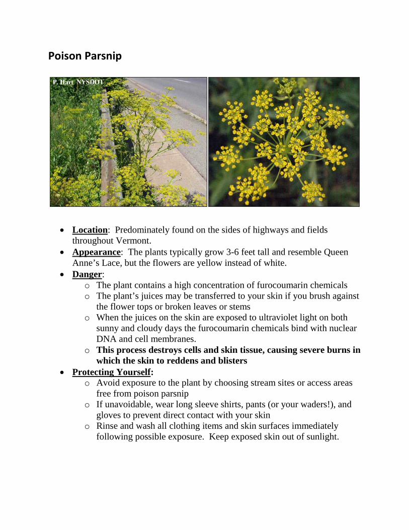
Poison Parsnip

• Location: Predominately found on the sides of highways and fields throughout Vermont.

• Appearance: The plants typically grow 3-6 feet tall and resemble Queen Anne’s Lace, but the flowers are yellow instead of white.

• Danger: o The plant contains a high concentration of furocoumarin chemicals o The plant’s juices may be transferred to your skin if you brush against

the flower tops or broken leaves or stems o When the juices on the skin are exposed to ultraviolet light on both

sunny and cloudy days the furocoumarin chemicals bind with nuclear DNA and cell membranes.

o This process destroys cells and skin tissue, causing severe burns in which the skin to reddens and blisters

• Protecting Yourself: o Avoid exposure to the plant by choosing stream sites or access areas

free from poison parsnip o If unavoidable, wear long sleeve shirts, pants (or your waders!), and

gloves to prevent direct contact with your skin o Rinse and wash all clothing items and skin surfaces immediately

following possible exposure. Keep exposed skin out of sunlight.

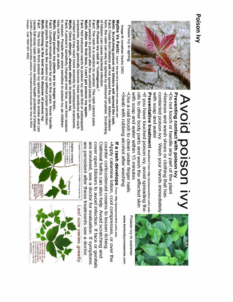
Poison Ivy

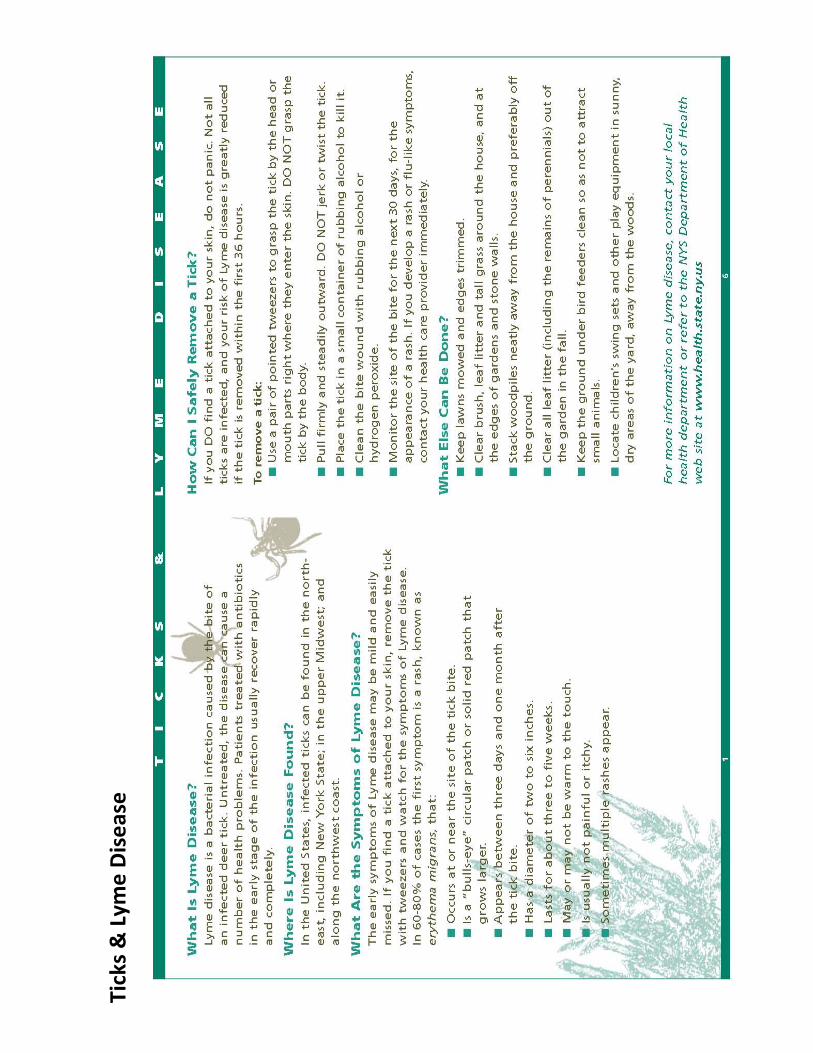
Tick

s & L

yme

Dis

ease

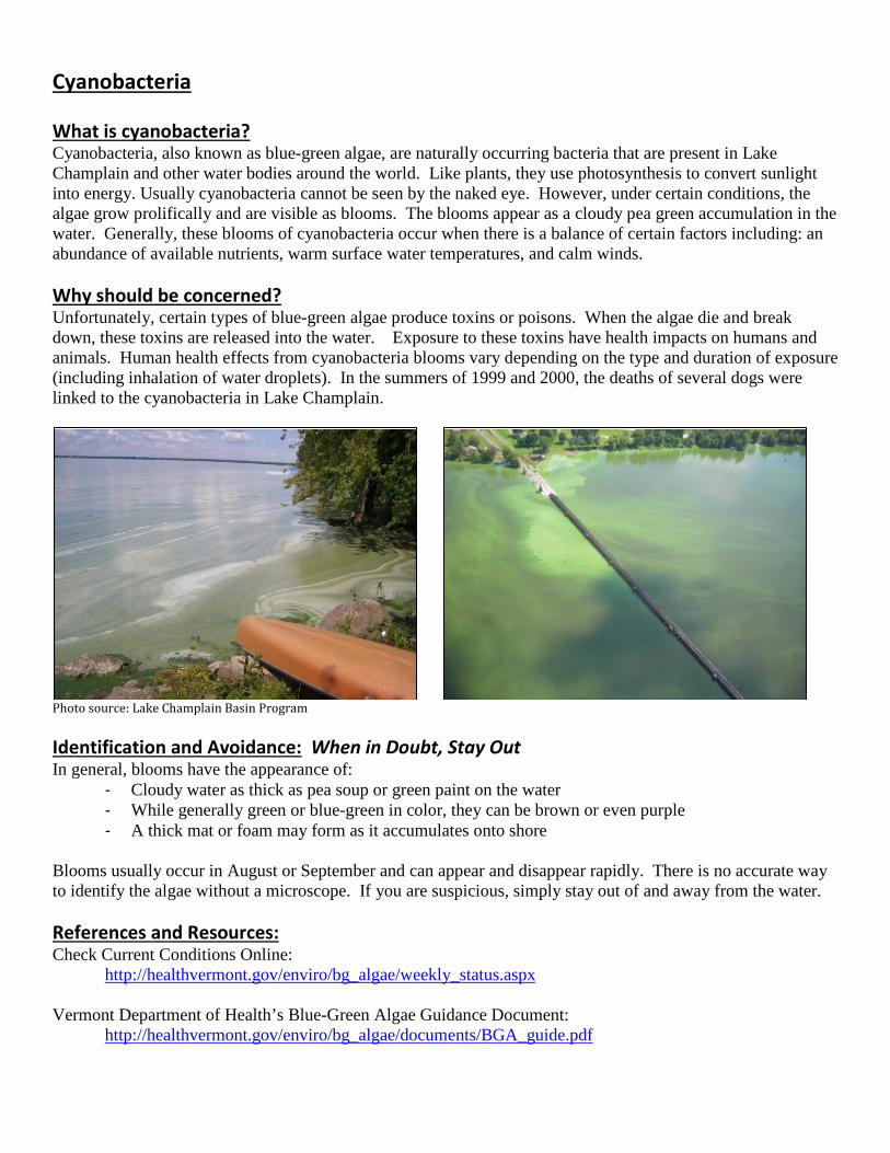
Cyanobacteria What is cyanobacteria? Cyanobacteria, also known as blue-green algae, are naturally occurring bacteria that are present in Lake Champlain and other water bodies around the world. Like plants, they use photosynthesis to convert sunlight into energy. Usually cyanobacteria cannot be seen by the naked eye. However, under certain conditions, the algae grow prolifically and are visible as blooms. The blooms appear as a cloudy pea green accumulation in the water. Generally, these blooms of cyanobacteria occur when there is a balance of certain factors including: an abundance of available nutrients, warm surface water temperatures, and calm winds. Why should be concerned? Unfortunately, certain types of blue-green algae produce toxins or poisons. When the algae die and break down, these toxins are released into the water. Exposure to these toxins have health impacts on humans and animals. Human health effects from cyanobacteria blooms vary depending on the type and duration of exposure (including inhalation of water droplets). In the summers of 1999 and 2000, the deaths of several dogs were linked to the cyanobacteria in Lake Champlain.

Photo source: Lake Champlain Basin Program Identification and Avoidance: When in Doubt, Stay Out In general, blooms have the appearance of:

- Cloudy water as thick as pea soup or green paint on the water - While generally green or blue-green in color, they can be brown or even purple - A thick mat or foam may form as it accumulates onto shore

Blooms usually occur in August or September and can appear and disappear rapidly. There is no accurate way to identify the algae without a microscope. If you are suspicious, simply stay out of and away from the water. References and Resources: Check Current Conditions Online:

http://healthvermont.gov/enviro/bg_algae/weekly_status.aspx Vermont Department of Health’s Blue-Green Algae Guidance Document:

http://healthvermont.gov/enviro/bg_algae/documents/BGA_guide.pdf

Websites: http://healthvermont.gov/enviro/bg_algae/bgalgae.aspx http://www.lcbp.org/water-environment/human-health/cyanobacteria/ http://www.lakechamplaincommittee.org/lcc-at-work/algae-in-lake/

Photo Galleries:

http://www.lcbp.org/2012/12/photo-gallery-2008-cyanobacteria-blooms/ http://healthvermont.gov/enviro/bg_algae/photos.aspx#bg

Report a Blue-green Algae Bloom: If you have questions or want to report a suspected bloom: Call 1-800-439-8550 or 802-863-7220, or email AHS.VDHBlueGreenAlgae@state.vt.us If you believe that someone has become ill because of exposure to blue-green algae, seek medical attention and contact the Health Department at 1-800-439-8550.

Journal of Great Lakes Research 38 (2012) 6–18

Contents lists available at SciVerse ScienceDirect

Journal of Great Lakes Research

j ourna l homepage: www.e lsev ie r .com/ locate / jg l r

Environmental change in Lake Champlain revealed by long-term monitoring

Eric Smeltzer a,⁎, Angela d. Shambaugh a,1, Pete Stangel b,2

a Vermont Department of Environmental Conservation, Watershed Management Division, 103 South Main St., Waterbury, VT 05671, USAb Lake Champlain Basin Program, Vermont Department of Environmental Conservation, Watershed Management Division, 103 South Main St., Waterbury, VT 05671, USA

⁎ Corresponding author. Tel.: +1 802 338 4840.E-mail addresses: eric.smeltzer@state.vt.us (E. Smelt

angela.shambaugh@state.vt.us (A. Shambaugh), pete.sta1 Tel.: +1 802 338 4821.2 Tel.: +1 802 654 8958.

0380-1330/$ – see front matter © 2012 International Adoi:10.1016/j.jglr.2012.01.002

a b s t r a c t

a r t i c l e i n f o

Article history:Received 28 September 2010Accepted 4 January 2012Available online 31 January 2012

Communicated by J. Ellen Marsden

Keywords:Lake ChamplainSecchiPhosphorusNitrogenChlorideDreissena

Long-term monitoring data on Lake Champlain spanning the past two to five decades were analyzed to docu-mentwater quality and biological changes in the lake. Augustmean surfacewater temperatures increased during1964–2009 inmost Lake Champlain regions at rates (0.035–0.085 °C/year) similar to what has been observed inthe LaurentianGreat Lakes and elsewhere. Secchi disk transparency increased by over ameter during 1964–2009in regions along the main stem of the lake, with much of the increase occurring after the 1993 zebra mussel in-vasion. Transparency declined in northeastern regions where zebra mussel densities were lower. No trends inhypolimnetic dissolved oxygen concentrations or depletion rateswere found in any of the deep lake regions during1990–2009. Sodium concentrations tripled in the Main Lake region since the 1960s. Chloride increased in theMain Lake by 30% since 1992, but declined in northeastern regions of the lake during recent years, coincidentwith reductions in road salt use in Vermont. Total phosphorus concentrations decreased during 1979–2009in southern and northwestern lake regions, but increased by 72% in Missisquoi Bay where chlorophyll-aconcentrations doubled over the period. There was a general lakewide trend of decreasing total nitrogenlevels during 1992–2009 that may have been due in part to reductions in atmospheric nitrogen loadingto the watershed. Cyanobacteria increased their dominance within the phytoplankton community innortheastern regions of the lake since the 1970s.

© 2012 International Association for Great Lakes Research. Published by Elsevier B.V. All rights reserved.

Introduction

Awareness of environmental change, and an understanding ofthe response of ecosystems to air and water pollution and land-usechanges, are essential to designing appropriate management inter-ventions (Lovett et al., 2007; Watzin, 2007). Because the rate ofmost ecological changes is very slow, usually occurring over decadesto centuries, long-term environmental monitoring is essential fordetecting trends in ecological variables.

Lakes are often the subject of long-termmonitoring because repre-sentative samples can be readily obtained that integrate the influence ofwatershed and atmospheric disturbances (Schindler, 2009). Importantknowledge has been gained from long-term monitoring of large lakes,including insights about lake ecosystem response to nutrient loadings,invasions by nonnative species, and climate change (Eimers et al.,2005; Rockwell et al., 2005; Jankowski et al., 2006; Dobiesz and Lester,2009; Fahnenstiel et al., 2010; Mida et al., 2010). In some cases, long-term lake monitoring data were used for purposes that were unfore-seeable at the time the monitoring program was initiated(Hampton et al., 2008).

zer),ngel@state.vt.us (P. Stangel).

ssociation for Great Lakes Research.

Lake Champlain is one of the largest lakes in North America, with a1127 km2 surface area, a mean depth of 22 m, and a 21,326 km2

drainage basin that are shared by the States of Vermont and NewYork and the Province of Quebec (Cohn et al., 2007). The lake has acomplex morphology with numerous shallow bays and arms thatare partially isolated from the deep main stem of the lake by naturalland forms or causeways. As a result, a wide variety of limnologicalconditions exists in Lake Champlain with respect to phosphorusloadings and trophic state (Medalie and Smeltzer, 2004), ionic com-position (Potash et al., 1969), thermal and hydrodynamic features(Manley et al., 1999), optical properties (Effler et al., 1991), and planktoncommunities (Shambaugh et al., 1999).

Like many large lakes worldwide, Lake Champlain faces a numberof environmental stressors. Global climate change, land use changes,agricultural and industrial contaminants in water runoff, and increasedopportunities for transport of exotic species all have the potential tosubstantially alter lake ecosystems. A substantial proportion of theLake Champlain drainage was deforested in the 1800s and convertedto farmland, leading to increased erosion and anthropogenic inputsof fertilizers. In comparison with the Great Lakes, the Lake Cham-plain Basin has a relatively low human population density and fewmajor industrial discharges. Similarly, the lake does not receivesubstantial shipping traffic, which is a major vector of exotic speciesintroductions in the Great Lakes and elsewhere. However, there areseveral stressors affecting the Lake Champlain Basin that would beexpected to produce environmental changes within the lake.

Published by Elsevier B.V. All rights reserved.

7E. Smeltzer et al. / Journal of Great Lakes Research 38 (2012) 6–18

Water temperature increases in large lakes have provided evidenceof a warming global climate (Dobiesz and Lester, 2009; Austin andColman, 2007; Hampton et al., 2008). Summer air temperatures haveincreased in the Lake Champlain region over the past several decades(Stager and Thill, 2010, Fig. 1a), and we would expect summer lakewater temperatures to have increased in Lake Champlain as a result.

Increasing chloride concentrations have been found in lakes(Chapra et al., 2009; Novotny and Stefan, 2009), rivers (Robinsonet al., 2003; Kauschal et al., 2005), and groundwater (Mullaney et al.,

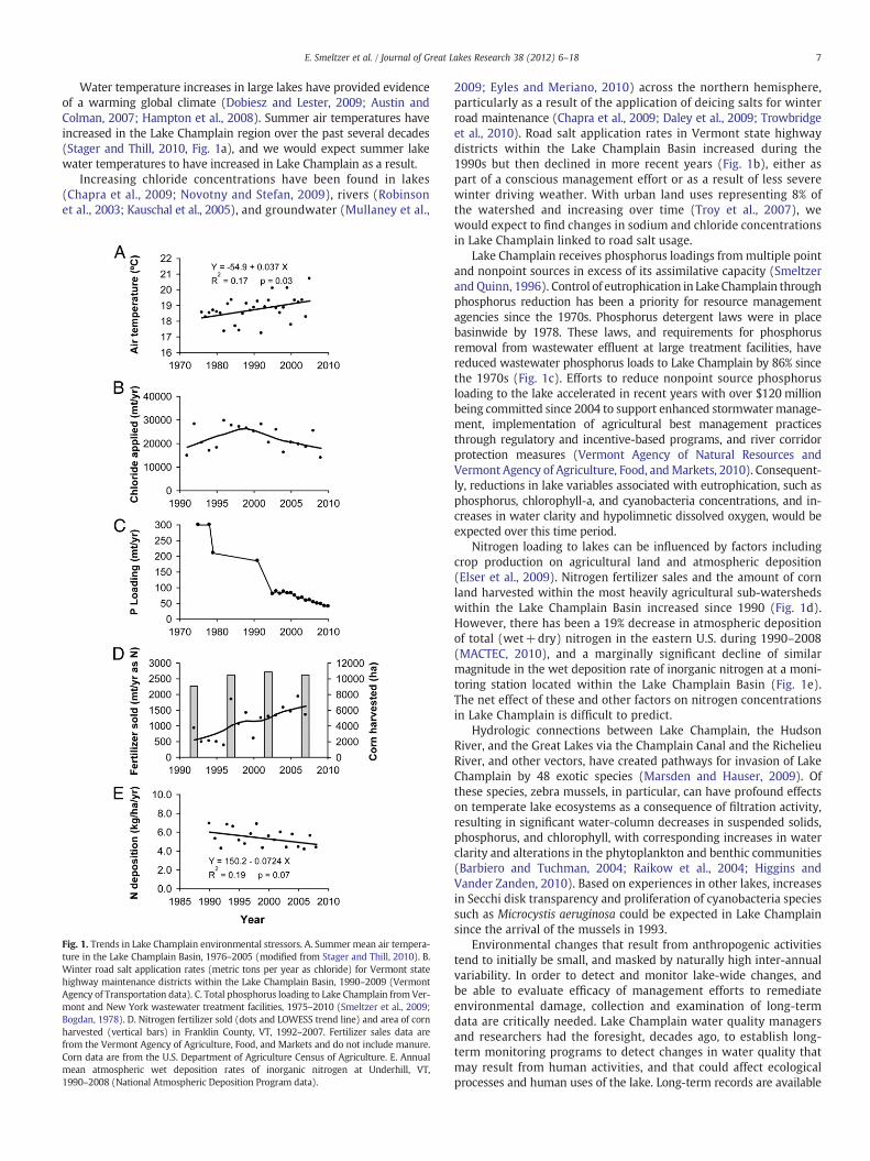
Fig. 1. Trends in Lake Champlain environmental stressors. A. Summer mean air tempera-ture in the Lake Champlain Basin, 1976–2005 (modified from Stager and Thill, 2010). B.Winter road salt application rates (metric tons per year as chloride) for Vermont statehighway maintenance districts within the Lake Champlain Basin, 1990–2009 (VermontAgency of Transportation data). C. Total phosphorus loading to Lake Champlain from Ver-mont and New York wastewater treatment facilities, 1975–2010 (Smeltzer et al., 2009;Bogdan, 1978). D. Nitrogen fertilizer sold (dots and LOWESS trend line) and area of cornharvested (vertical bars) in Franklin County, VT, 1992–2007. Fertilizer sales data arefrom the Vermont Agency of Agriculture, Food, and Markets and do not include manure.Corn data are from the U.S. Department of Agriculture Census of Agriculture. E. Annualmean atmospheric wet deposition rates of inorganic nitrogen at Underhill, VT,1990–2008 (National Atmospheric Deposition Program data).

2009; Eyles and Meriano, 2010) across the northern hemisphere,particularly as a result of the application of deicing salts for winterroad maintenance (Chapra et al., 2009; Daley et al., 2009; Trowbridgeet al., 2010). Road salt application rates in Vermont state highwaydistricts within the Lake Champlain Basin increased during the1990s but then declined in more recent years (Fig. 1b), either aspart of a conscious management effort or as a result of less severewinter driving weather. With urban land uses representing 8% ofthe watershed and increasing over time (Troy et al., 2007), wewould expect to find changes in sodium and chloride concentrationsin Lake Champlain linked to road salt usage.

Lake Champlain receives phosphorus loadings frommultiple pointand nonpoint sources in excess of its assimilative capacity (Smeltzerand Quinn, 1996). Control of eutrophication in LakeChamplain throughphosphorus reduction has been a priority for resource managementagencies since the 1970s. Phosphorus detergent laws were in placebasinwide by 1978. These laws, and requirements for phosphorusremoval from wastewater effluent at large treatment facilities, havereduced wastewater phosphorus loads to Lake Champlain by 86% sincethe 1970s (Fig. 1c). Efforts to reduce nonpoint source phosphorusloading to the lake accelerated in recent years with over $120 millionbeing committed since 2004 to support enhanced stormwater manage-ment, implementation of agricultural best management practicesthrough regulatory and incentive-based programs, and river corridorprotection measures (Vermont Agency of Natural Resources andVermont Agency of Agriculture, Food, andMarkets, 2010). Consequent-ly, reductions in lake variables associated with eutrophication, such asphosphorus, chlorophyll-a, and cyanobacteria concentrations, and in-creases in water clarity and hypolimnetic dissolved oxygen, would beexpected over this time period.

Nitrogen loading to lakes can be influenced by factors includingcrop production on agricultural land and atmospheric deposition(Elser et al., 2009). Nitrogen fertilizer sales and the amount of cornland harvested within the most heavily agricultural sub-watershedswithin the Lake Champlain Basin increased since 1990 (Fig. 1d).However, there has been a 19% decrease in atmospheric depositionof total (wet+dry) nitrogen in the eastern U.S. during 1990–2008(MACTEC, 2010), and a marginally significant decline of similarmagnitude in the wet deposition rate of inorganic nitrogen at a moni-toring station located within the Lake Champlain Basin (Fig. 1e).The net effect of these and other factors on nitrogen concentrationsin Lake Champlain is difficult to predict.

Hydrologic connections between Lake Champlain, the HudsonRiver, and the Great Lakes via the Champlain Canal and the RichelieuRiver, and other vectors, have created pathways for invasion of LakeChamplain by 48 exotic species (Marsden and Hauser, 2009). Ofthese species, zebra mussels, in particular, can have profound effectson temperate lake ecosystems as a consequence of filtration activity,resulting in significant water-column decreases in suspended solids,phosphorus, and chlorophyll, with corresponding increases in waterclarity and alterations in the phytoplankton and benthic communities(Barbiero and Tuchman, 2004; Raikow et al., 2004; Higgins andVander Zanden, 2010). Based on experiences in other lakes, increasesin Secchi disk transparency and proliferation of cyanobacteria speciessuch as Microcystis aeruginosa could be expected in Lake Champlainsince the arrival of the mussels in 1993.

Environmental changes that result from anthropogenic activitiestend to initially be small, and masked by naturally high inter-annualvariability. In order to detect and monitor lake-wide changes, andbe able to evaluate efficacy of management efforts to remediateenvironmental damage, collection and examination of long-termdata are critically needed. Lake Champlain water quality managersand researchers had the foresight, decades ago, to establish long-term monitoring programs to detect changes in water quality thatmay result from human activities, and that could affect ecologicalprocesses and human uses of the lake. Long-term records are available

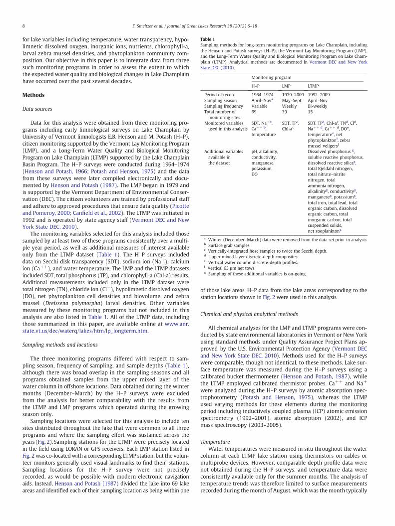
Table 1Sampling methods for long-term monitoring programs on Lake Champlain, includingthe Henson and Potash surveys (H–P), the Vermont Lay Monitoring Program (LMP),and the Long-Term Water Quality and Biological Monitoring Program on Lake Cham-plain (LTMP). Analytical methods are documented in Vermont DEC and New YorkState DEC (2010).

Monitoring program

H–P LMP LTMP

Period of record 1964–1974 1979–2009 1992–2009Sampling season April–Nova May–Sept April–NovSampling frequency Variable Weekly Bi-weeklyTotal number ofmonitoring sites

69 39 15

Monitored variablesused in this analysis

SDT, Na+b,Ca++ b,temperature

SDT, TPc,Chl-ac

SDT, TPd, Chl-ac, TNd, Cld,Na++ d, Ca++ d, DOe,temperaturee, netphytoplanktonf, zebramussel veligersf

Additional variablesavailable inthe dataset

pH, alkalinity,conductivity,manganese,potassium,DO

Dissolved phosphorus g,soluble reactive phosphorus,dissolved reactive silicag,total Kjeldahl nitrogen,total nitrate–nitritenitrogen, totalammonia nitrogen,alkalinityg, conductivityg,manganeseg, potassiumg,total iron, total lead, totalorganic carbon, dissolvedorganic carbon, totalinorganic carbon, totalsuspended solids,net zooplanktong

a Winter (December–March) data were removed from the data set prior to analysis.b Surface grab samples.c Vertically-integrated hose samples to twice the Secchi depth.d Upper mixed layer discrete-depth composites.e Vertical water column discrete-depth profiles.f Vertical 63 µm net tows.g Sampling of these additional variables is on-going.

8 E. Smeltzer et al. / Journal of Great Lakes Research 38 (2012) 6–18

for lake variables including temperature, water transparency, hypo-limnetic dissolved oxygen, inorganic ions, nutrients, chlorophyll-a,larval zebra mussel densities, and phytoplankton community com-position. Our objective in this paper is to integrate data from threesuch monitoring programs in order to assess the extent to whichthe expected water quality and biological changes in Lake Champlainhave occurred over the past several decades.

Methods

Data sources

Data for this analysis were obtained from three monitoring pro-grams including early limnological surveys on Lake Champlain byUniversity of Vermont limnologists E.B. Henson and M. Potash (H–P),citizen monitoring supported by the Vermont Lay Monitoring Program(LMP), and a Long-Term Water Quality and Biological MonitoringProgram on Lake Champlain (LTMP) supported by the Lake ChamplainBasin Program. The H–P surveys were conducted during 1964–1974(Henson and Potash, 1966; Potash and Henson, 1975) and the datafrom these surveys were later compiled electronically and docu-mented by Henson and Potash (1987). The LMP began in 1979 andis supported by the Vermont Department of Environmental Conser-vation (DEC). The citizen volunteers are trained by professional staffand adhere to approved procedures that ensure data quality (Picotteand Pomeroy, 2000; Canfield et al., 2002). The LTMP was initiated in1992 and is operated by state agency staff (Vermont DEC and NewYork State DEC, 2010).

The monitoring variables selected for this analysis included thosesampled by at least two of these programs consistently over a multi-ple year period, as well as additional measures of interest availableonly from the LTMP dataset (Table 1). The H–P surveys includeddata on Secchi disk transparency (SDT), sodium ion (Na+), calciumion (Ca++), and water temperature. The LMP and the LTMP datasetsincluded SDT, total phosphorus (TP), and chlorophyll-a (Chl-a) results.Additional measurements included only in the LTMP dataset weretotal nitrogen (TN), chloride ion (Cl−), hypolimnetic dissolved oxygen(DO), net phytoplankton cell densities and biovolume, and zebramussel (Dreissena polymorpha) larval densities. Other variablesmeasured by these monitoring programs but not included in thisanalysis are also listed in Table 1. All of the LTMP data, includingthose summarized in this paper, are available online at www.anr.state.vt.us/dec/waterq/lakes/htm/lp_longterm.htm.

Sampling methods and locations

The three monitoring programs differed with respect to sam-pling season, frequency of sampling, and sample depths (Table 1),although there was broad overlap in the sampling seasons and allprograms obtained samples from the upper mixed layer of thewater column in offshore locations. Data obtained during the wintermonths (December–March) by the H–P surveys were excludedfrom the analysis for better comparability with the results fromthe LTMP and LMP programs which operated during the growingseason only.

Sampling locations were selected for this analysis to include tensites distributed throughout the lake that were common to all threeprograms and where the sampling effort was sustained across theyears (Fig. 2). Sampling stations for the LTMP were precisely locatedin the field using LORAN or GPS receivers. Each LMP station listed inFig. 2 was co-locatedwith a corresponding LTMP station, but the volun-teer monitors generally used visual landmarks to find their stations.Sampling locations for the H–P survey were not preciselyrecorded, as would be possible with modern electronic navigationaids. Instead, Henson and Potash (1987) divided the lake into 69 lakeareas and identified each of their sampling location as being within one

of those lake areas. H–P data from the lake areas corresponding to thestation locations shown in Fig. 2 were used in this analysis.

Chemical and physical analytical methods

All chemical analyses for the LMP and LTMP programs were con-ducted by state environmental laboratories in Vermont or New Yorkusing standard methods under Quality Assurance Project Plans ap-proved by the U.S. Environmental Protection Agency (Vermont DECand New York State DEC, 2010). Methods used for the H–P surveyswere comparable, though not identical, to these methods. Lake sur-face temperature was measured during the H–P surveys using acalibrated bucket thermometer (Henson and Potash, 1987), whilethe LTMP employed calibrated thermistor probes. Ca++ and Na+

were analyzed during the H–P surveys by atomic absorption spec-trophotometry (Potash and Henson, 1975), whereas the LTMPused varying methods for these elements during the monitoringperiod including inductively coupled plasma (ICP) atomic emissionspectrometry (1992–2001), atomic absorption (2002), and ICPmass spectroscopy (2003–2005).

TemperatureWater temperatures were measured in situ throughout the water

column at each LTMP lake station using thermistors on cables ormultiprobe devices. However, comparable depth profile data werenot obtained during the H–P surveys, and temperature data wereconsistently available only for the summer months. The analysis oftemperature trends was therefore limited to surface measurementsrecorded during themonth of August, whichwas themonth typically

Fig. 2. Location of sampling stations in Lake Champlain. Stations sampled by the H–Psurveys were not precisely located, but corresponded to the general lake regionindicated.

9E. Smeltzer et al. / Journal of Great Lakes Research 38 (2012) 6–18

having the largest number of measurements. All temperaturesrecorded at 1 m depth during August (N=1–5/year) were averagedby year to calculate an August mean surface temperature in each lakeregion for years where data were available.

Hypolimnetic dissolved oxygenHypolimnetic DO was measured by the LTMP using both Winkler

titration and in situ electrode methods (Vermont DEC and NewYork State DEC, 2010). However, several different instruments wereemployed across the years for the electrode measurements and theWinkler method provided more consistently calibrated data overthe entire monitoring period. Therefore, only the Winkler titrationresults were used for long-term trends analysis.

Conventional measures of hypolimnetic hypoxia such as the arealor volumetric hypolimnetic oxygen depletion rate (Burns et al.,2005; Matthews and Effler, 2006) were difficult to apply to LakeChamplain because the complex morphometry and sometimes in-distinct thermocline created uncertainty about the spatial extent ofthe hypolimnion at some sampling stations. Trends in hypolimnetichypoxia were assessed instead using measurements of late-summerDO concentrations recorded by the LTMP in the near-bottom watersof three deep lake regions, including the Main Lake (90 m), MallettsBay (25 m), and the Northeast Arm (45 m). In order to standardizethe comparison of late-summer DO conditions across years, DO con-centrations were interpolated between sampling dates to providean estimate of the DO concentration at these depths on September1 of each year. Additionally, summer-long hypolimnetic DO depletionrates were calculated from the differences in bottom-water DO con-centrations between June 1 and September 1 each year. The depthlocations of the hypolimnetic DO samples used for this analysiswere the same across all years within each lake region. DO dataobtained during 1990–1991 by a preceding study using comparablemethods (Vermont DEC and New York State DEC, 1997) were usedto supplement the LTMP dataset for this analysis.

Zebra mussel veligersZebra mussel adults were first discovered in the South Lake region

of Lake Champlain in 1993, and their planktonic larvae (veligers)were monitored by the LTMP starting in 1994 to provide an indirectmeasure of population densities as the mussels spread to other regionsof the lake. Zebra mussel veligers were sampled by vertical net towsconcurrently with the water quality monitoring efforts (Stangel andShambaugh, 2005). Tow depths varied between 3 and 10 m dependingon the depth of the sampling station. Enumeration procedures fol-lowed Marsden (1992). The seasonal timing of veliger productionvaried from site to site and year to year. In order to provide a stan-dardized basis for comparison, veliger densities at each station werereported as a time-weighted season mean calculated by numericallyintegrating the measured densities over 150-day periods within eachMay–October sampling season, starting and ending with zero densityobservations (Stangel and Shambaugh, 2005).

PhytoplanktonLarge phytoplankton were sampled by the LTMP beginning in

2006 using a 63 μm mesh Wisconsin net. Samples were collected byvertical net tows from twice the Secchi depth and preserved withacid Lugol's solution for later analysis. Individuals with at leastone linear dimension >50 μm were identified to the lowest taxo-nomic level practical and enumerated. Ten randomly selected in-dividuals from each taxon were measured and the median valuesof these dimensions were used with standard geometric formu-lae to determine a representative biovolume per cell (Wetzel andLikens, 2000).

Statistical analysis

All sampling results were averaged for each date to reduce fieldreplicates to a single value per sampling date. Locally weightedscatterplot smoothing (LOWESS) was used to visualize temporaltrends in the data including any non-linearity, while illustratingthe variability in the data. LOWESS identifies the centerline of thetime series plots, illustrating the underlying trends amidst the con-siderable variability present in the data (Helsel and Hirsch, 2005).Regression window widths for weighting were controlled usingmoderate smoothness values of 0.4–0.6 for most variables in thisanalysis.

One of the concerns about using data from monitoring programswith different sampling methods operating over different time pe-riods (Table 1) is the potential for an apparent temporal trend to be

10 E. Smeltzer et al. / Journal of Great Lakes Research 38 (2012) 6–18

an artifact of methodological differences. To check for such differ-ences and minimize the influence of method artifacts, annual meanvalues for STD, TP, and Chl-a were calculated from data that werelog-transformed for normality for all lake stations and years thatwere sampled concurrently by the LMP and LTMP programs. A pairedt-test (pb0.05) was used to test the statistical significance of anydifferences between these two sampling programs in the distribu-tions of the annual means for each lake station and water qualityvariable. Where significant differences were found, separate LOWESScurves were fit to data from the LMP and LTMP programs and shownin parallel. Since the H–P surveys did not overlap in time with theother two monitoring programs, it was not possible to test for bias inthe H–P results relative to the LMP or LTMP data.

The statistical significance of temporal trends suggested by theLOWESS plots was tested by linear regression of concentration vs.time in decimal years over the entire monitoring period. Means ofthe annual mean values were compared between the LMP andLTMP for each variable and lake station. For any variable and lakestation found to be significantly different between the two programsduring concurrent time periods, indicating possible programmaticbias, data from the LMP only were retained for the regressionsbecause of the longer period of record from this program, and LTMPresults were excluded. Unless noted otherwise, trends reported inthe results as “increasing” or “decreasing” had slopes that were signif-icantly different from zero (pb0.05), based on the linear regressionanalysis.

Intervals between sampling events within a particular lake regionwere typically a week or more, but the potential for temporal auto-correlation and overstated statistical significance of the regressionresults exists. While not tested, the influence of possible temporalautocorrelation on the general findings of these analyses is likely tobe small because most regressions noted as statistically significanthad p values well below the 0.05 criterion.

Results and discussion

Temperature

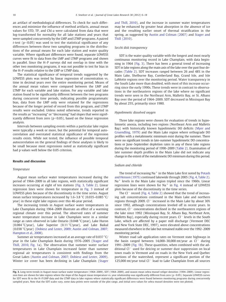
August mean surface water temperatures increased during theperiod of 1964–2009 in all lake regions, with statistically significantincreases occurring at eight of ten stations (Fig. 3, Table 2). Linearregression lines were shown for temperature in Fig. 3 instead ofLOWESS plots because of the discontinuity in the time series. Augustmean surface temperatures increased by 1.6–3.8 °C (0.035–0.085 °C/year) in these eight lake regions over this 46-year period.

The increasing trends in August surface water temperatures inLake Champlain during 1964–2009 illustrate an effect of a warmingregional climate over this period. The observed rates of summerwater temperature increase in Lake Champlain were in a similarrange as rates observed in Lake Ontario (0.048 °C/year), Lake Huron(0.084 °C/year), Lake Superior (0.11 °C/year), and Lake Baikal(0.038 °C/year) (Dobiesz and Lester, 2009; Austin and Colman, 2007;Hampton et al., 2008).

Summer air temperatures increased at an average rate of 0.037 °C/year in the Lake Champlain Basin during 1976–2005 (Stager andThill, 2010, Fig. 1a). The observation that summer water surfacetemperatures in Lake Champlain increased faster than summerregional air temperatures is consistent with findings from theGreat Lakes (Austin and Colman, 2007; Dobiesz and Lester, 2009).Winter ice cover has been declining in Lake Champlain (Stager

Fig. 3. Long-term trends in August mean surface water temperature (1964–2009), SDT (196sion lines are shown for lake regions where the slope of the August mean temperature vs. yefor SDT were fit to the H–P/LMP data and the LTMP data in lake regions where statisticallysampled years. Note that the SDT scales vary, some data points were outside of the plot ran

and Thill, 2010), and the increase in summer water temperaturesmay be enhanced by greater heat absorption in the absence of iceand the resulting earlier onset of thermal stratification in thespring, as suggested by Austin and Colman (2007) and Stager andThill (2010).

Secchi disk transparency

SDT is the water quality variable with the longest and most nearlycontinuous monitoring record in Lake Champlain, with data begin-ning in 1964 (Fig. 3). There has been a general trend of increasingSDT in lake regions along themain axis of the lake over the past four de-cades (Table 2). SDT increases ranged between 26 and 48% in theMain Lake, Shelburne Bay, Cumberland Bay, Grand Isle, and IsleLaMotte regions over the monitoring period. Water transparency inthe South Lake more than doubled, with most of this increase occur-ring since the early 1990s. These trends were in contrast to observa-tions in the northeastern regions of the lake where no significanttrends were seen in the Northeast Arm, Malletts Bay, or St. AlbansBay over the period of 1964–2009. SDT decreased in Missisquoi Bayby about 25%, primarily since 1980.

Hypolimnetic dissolved oxygen

Three lake regions were chosen for evaluation of trends in hypo-limnetic anoxia, including two regions (Northeast Arm and MallettsBay) with historically known hypolimnetic DO deficits (Myer andGruendling, 1979) and the Main Lake region where orthograde DOprofiles with a metalimnetic minimum exist during the summer. Therewere no significant trends in late-summer hypolimnetic DO concentra-tions or June–September depletion rates in any of these lake regionsduring the monitoring period of 1990–2009 (Table 2). Examination oflate summer depth profiles in the Main Lake did not indicate anychange in the extent of themetalimnetic DOminimumduring this period.

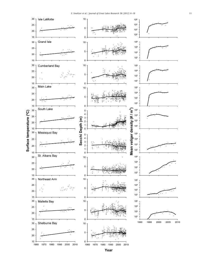
Sodium and chloride

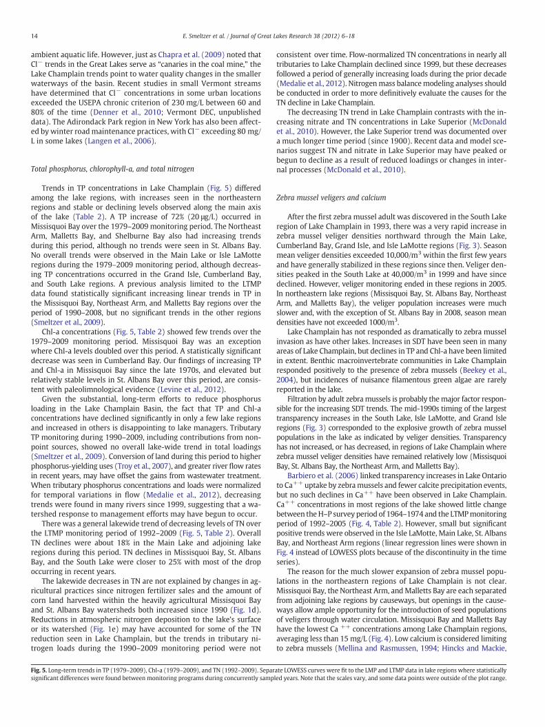
The trend of increasing Na+ in the Main Lake first noted by PotashandHenson (1975) continued lakewide through 2005 (Fig. 4, Table 2).Na+ levels in the Main Lake region tripled since the 1960s. Linearregression lines were shown for Na+ in Fig. 4 instead of LOWESSplots because of the discontinuity in the time series.

The Cl− record (Fig. 4, Table 2) showed that the trend of increas-ing salt concentrations continued in the Main Lake and northernregions through 2009. Cl− increased in the Main Lake by about 30%since 1992, although concentrations leveled off in recent years. Incontrast, Cl− concentrations declined in the northeastern regions ofthe lake since 1992 (Missisquoi Bay, St. Albans Bay, Northeast Arm,Malletts Bay), especially during recent years. Cl− levels in the SouthLake, which are affected by a paper mill discharge (Vermont DECand New York State DEC, 1997), were elevated above concentrationsmeasured elsewhere in the lake but remained stable over the 1992–2009monitoring period.

Winter road salt application rates on Vermont state highways inthe basin ranged between 14,000–30,000 mt/year as Cl− during1991–2009 (Fig. 1b). These quantities, when combined with the ad-ditional Cl− used for deicing or summer dust suppression on localtown roads in Vermont and on roads in the New York and Quebecportions of the watershed, represent a significant portion of the125,000 mt/year total Cl− load to Lake Champlain from all sources

4–2009), and season mean zebra mussel veliger densities (1994–2009). Linear regres-ar relationship was significantly different from zero (pb0.05). Separate LOWESS curvessignificant differences were found between monitoring programs during concurrentlyge, and initial zero values for zebra mussel densities were not plotted.

11E. Smeltzer et al. / Journal of Great Lakes Research 38 (2012) 6–18

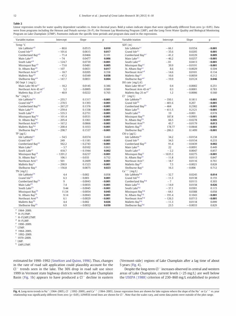
Table 2Linear regression results for water quality dependent variables vs. time in decimal years. Bold p values indicate slopes that were significantly different from zero (pb0.05). Datawere from programs including the Henson and Potash surveys (H–P), the Vermont Lay Monitoring Program (LMP), and the Long-Term Water Quality and Biological MonitoringProgram on Lake Champlain (LTMP). Footnotes indicate the specific time periods and program data used in the regressions.

Variable/station Intercept Slope p Variable/station Intercept Slope p

Temp °C SDT (m)Isle LaMottea,b −80.6 0.0515 0.010 Isle LaMottea,c −66.1 0.0354 b0.001Grand Islea,b −101.6 0.0615 0.017 Grand Islea,c −35.6 0.0205 0.001Cumberland Baya,b −71.4 0.0466 0.101 Cumberland Baya,c −41.2 0.0229 0.005Main Lakea,b −74 0.0477 0.006 Main Lakea,c −46.2 0.0257 b0.001South Lakea,b −124.7 0.0739 b0.001 South Lakea,d −81 0.0413 b0.001Missisquoi Baya,b −73.6 0.0481 0.005 Missisquoi Baya,c 39.9 −0.0191 b0.001St. Albans Baya,b −107 0.0651 0.017 St. Albans Baya,c 8.6 −0.0029 0.504Northeast Arma,b −18.7 0.0205 0.358 Northeast Arma,d −14.6 0.0101 0.134Malletts Baya,b −47.2 0.0349 0.038 Malletts Baya,c 16.6 −0.0059 0.212Shelburne Baya,b −147.7 0.0851 0.004 Shelburne Baya,d −19.9 0.0124 0.046

DO Sept 1 (mg/L) DO rate (mg/L/d)Main Lake 90 me,f −18.2 0.0145 0.386 Main Lake 90 me,f 0.4 −0.0002 0.251Northeast Arm 45 me,f 5.2 −0.0005 0.989 Northeast Arm 45 me,f 0.3 −0.0001 0.783Malletts Bay 25 me,f −40.9 0.0222 0.765 Malletts Bay 25 me,f 1.2 −0.0006 0.560

Na+ (mg/L) Cl− (mg/L)Isle LaMotteb,g −255.7 0.1317 b0.001 Isle LaMottef,h −350.1 0.1811 b0.001Grand Isleb,g −270.5 0.1393 b0.001 Grand Islef,h −401.6 0.207 b0.001Cumberland Bayb,g −267.27 0.1376 b0.001 Cumberland Bayf,h −464 0.2382 b0.001Main Lakeb,g −259.4 0.1338 b0.001 Main Lakef,h −411.5 0.2121 b0.001South Lakeb,g −535.3 0.2751 b0.001 South Lakef,h 19 −0.001 0.978Missisquoi Bayb,g −101.4 0.0531 b0.001 Missisquoi Bayf,h 187.8 −0.0901 b0.001St. Albans Bayb,g −205.4 0.1061 b0.001 St. Albans Bayf,h 66.5 −0.0278 0.005Northeast Armb,g −167.2 0.0866 b0.001 Northeast Armf,h 45.7 −0.0179 0.013Malletts Bayb,g −200.4 0.1033 b0.001 Malletts Bayf,h 178.77 −0.0844 b0.001Shelburne Bayb,g −298.7 0.1537 b0.001 Shelburne Bayf,h −286.3 0.1499 b0.001

TP (μg/L) Chl-a (μg/L)Isle LaMottei,j −54.5 0.0374 0.460 Isle LaMottei,k 34.2 −0.0154 0.238Grand Islei,k 249 −0.1181 b0.001 Grand Islei,k 34.5 −0.0154 0.233Cumberland Bayi,k 562.2 −0.2743 b0.001 Cumberland Bayi,k 91.4 −0.0439 0.002Main Lakei,j −3.7 0.0102 0.863 Main Lakei,k 22 −0.0091 0.449South Lakei,j 418.7 −0.1944 0.002 South Lakei,k −2.2 0.0047 0.857Missisquoi Bayi,k −1201.2 0.6237 b0.001 Missisquoi Bayi,j −1635.3 0.8275 b0.001St. Albans Bayi,j 106.1 −0.035 0.752 St. Albans Bayi,k −11.8 0.0113 0.847Northeast Armi,j −501 0.2609 0.001 Northeast Armi,j −18.7 0.0116 0.761Malletts Bayi,j −290.9 0.1523 b0.001 Malletts Bayi,k 7.5 −0.0021 0.828Shelburne Bayi,j −156.8 0.0875 0.023 Shelburne Bayi,j 16.3 −0.006 0.712

TN (mg/L) Ca++ (mg/L)Isle LaMottef,h 4.4 −0.002 0.058 Isle LaMotteb,g −32.7 0.0245 0.014Grand Islef,h 6.3 −0.003 0.001 Grand Isleb,g −11.3 0.0138 0.155Cumberland Bayf,h 9 −0.0043 b0.001 Cumberland Bayb,g −7 0.0115 0.303Main Lakef,h 7.4 −0.0035 b0.001 Main Lakeb,g −14.9 0.0158 0.026South Lakef,h 9.44 −0.0045 b0.001 South Lakeb,g −37.1 0.0301 0.115Missisquoi Bayf,h 11.54 −0.0054 0.045 Missisquoi Bayb,g −64.1 0.0388 0.058St. Albans Bayf,h 9.14 −0.0043 0.001 St. Albans Bayb,g −191.4 0.1043 b0.001Northeast Armf,h 6.1 −0.0029 b0.001 Northeast Armb,g −126.3 0.0713 b0.001Malletts Bayf,h 4.4 −0.002 0.026 Malletts Bayb,g −11.3 0.0118 0.099Shelburne Bayf,h 6.9 −0.0032 0.030 Shelburne Bayb,g 23.5 −0.0033 0.829

a 1964–2009.b H–P,LTMP.c H–P,LMP,LTMP.d H–P,LMP.e 1990–2009.f LTMP.g 1964–2005.h 1992–2009.i 1979–2009.j LMP.k LMP,LTMP.

12 E. Smeltzer et al. / Journal of Great Lakes Research 38 (2012) 6–18

estimated for 1990–1992 (Smeltzer and Quinn, 1996). Thus, changesin the rate of road salt application could plausibly account for theCl− trends seen in the lake. The 30% drop in road salt use since1999 in Vermont state highway districts within the Lake ChamplainBasin (Fig. 1b) appears to have produced a Cl− decline in eastern

Fig. 4. Long-term trends in Na+ (1964–2005), Cl− (1992–2009), and Ca++ (1964–2005). Linerelationship was significantly different from zero (pb0.05). LOWESS trend lines are shown for

(Vermont-side) regions of Lake Champlain after a lag time of about5 years (Fig. 4).

Despite the long-term Cl− increases observed in central and westernareas of Lake Champlain, current levels (b25 mg/L) are well belowthe USEPA (1988) criterion of 230–860 mg/L established to protect

ar regression lines are shown for lake regions where the slope of the Na+ or Ca++ vs. yearCl−. Note that the scales vary, and some data points were outside of the plot range.

13E. Smeltzer et al. / Journal of Great Lakes Research 38 (2012) 6–18

14 E. Smeltzer et al. / Journal of Great Lakes Research 38 (2012) 6–18

ambient aquatic life. However, just as Chapra et al. (2009) noted thatCl− trends in the Great Lakes serve as “canaries in the coal mine,” theLake Champlain trends point to water quality changes in the smallerwaterways of the basin. Recent studies in small Vermont streamshave determined that Cl− concentrations in some urban locationsexceeded the USEPA chronic criterion of 230 mg/L between 60 and80% of the time (Denner et al., 2010; Vermont DEC, unpublisheddata). The Adirondack Park region in New York has also been affect-ed by winter roadmaintenance practices, with Cl− exceeding 80 mg/L in some lakes (Langen et al., 2006).

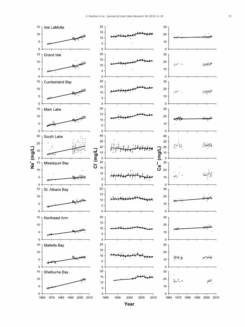
Total phosphorus, chlorophyll-a, and total nitrogen

Trends in TP concentrations in Lake Champlain (Fig. 5) differedamong the lake regions, with increases seen in the northeasternregions and stable or declining levels observed along the main axisof the lake (Table 2). A TP increase of 72% (20 μg/L) occurred inMissisquoi Bay over the 1979–2009 monitoring period. The NortheastArm, Malletts Bay, and Shelburne Bay also had increasing trendsduring this period, although no trends were seen in St. Albans Bay.No overall trends were observed in the Main Lake or Isle LaMotteregions during the 1979–2009 monitoring period, although decreas-ing TP concentrations occurred in the Grand Isle, Cumberland Bay,and South Lake regions. A previous analysis limited to the LTMPdata found statistically significant increasing linear trends in TP inthe Missisquoi Bay, Northeast Arm, and Malletts Bay regions over theperiod of 1990–2008, but no significant trends in the other regions(Smeltzer et al., 2009).

Chl-a concentrations (Fig. 5, Table 2) showed few trends over the1979–2009 monitoring period. Missisquoi Bay was an exceptionwhere Chl-a levels doubled over this period. A statistically significantdecrease was seen in Cumberland Bay. Our findings of increasing TPand Chl-a in Missisquoi Bay since the late 1970s, and elevated butrelatively stable levels in St. Albans Bay over this period, are consis-tent with paleolimnological evidence (Levine et al., 2012).

Given the substantial, long-term efforts to reduce phosphorusloading in the Lake Champlain Basin, the fact that TP and Chl-aconcentrations have declined significantly in only a few lake regionsand increased in others is disappointing to lake managers. TributaryTP monitoring during 1990–2009, including contributions from non-point sources, showed no overall lake-wide trend in total loadings(Smeltzer et al., 2009). Conversion of land during this period to higherphosphorus-yielding uses (Troy et al., 2007), and greater river flow ratesin recent years, may have offset the gains from wastewater treatment.When tributary phosphorus concentrations and loads were normalizedfor temporal variations in flow (Medalie et al., 2012), decreasingtrends were found in many rivers since 1999, suggesting that a wa-tershed response to management efforts may have begun to occur.

There was a general lakewide trend of decreasing levels of TN overthe LTMP monitoring period of 1992–2009 (Fig. 5, Table 2). OverallTN declines were about 18% in the Main Lake and adjoining lakeregions during this period. TN declines in Missisquoi Bay, St. AlbansBay, and the South Lake were closer to 25% with most of the dropoccurring in recent years.

The lakewide decreases in TN are not explained by changes in ag-ricultural practices since nitrogen fertilizer sales and the amount ofcorn land harvested within the heavily agricultural Missisquoi Bayand St. Albans Bay watersheds both increased since 1990 (Fig. 1d).Reductions in atmospheric nitrogen deposition to the lake's surfaceor its watershed (Fig. 1e) may have accounted for some of the TNreduction seen in Lake Champlain, but the trends in tributary ni-trogen loads during the 1990–2009 monitoring period were not

Fig. 5. Long-term trends in TP (1979–2009), Chl-a (1979–2009), and TN (1992–2009). Separsignificant differences were found between monitoring programs during concurrently samp

consistent over time. Flow-normalized TN concentrations in nearly alltributaries to Lake Champlain declined since 1999, but these decreasesfollowed a period of generally increasing loads during the prior decade(Medalie et al., 2012). Nitrogenmass balancemodeling analyses shouldbe conducted in order to more definitively evaluate the causes for theTN decline in Lake Champlain.

The decreasing TN trend in Lake Champlain contrasts with the in-creasing nitrate and TN concentrations in Lake Superior (McDonaldet al., 2010). However, the Lake Superior trend was documented overa much longer time period (since 1900). Recent data and model sce-narios suggest TN and nitrate in Lake Superior may have peaked orbegun to decline as a result of reduced loadings or changes in inter-nal processes (McDonald et al., 2010).

Zebra mussel veligers and calcium

After the first zebra mussel adult was discovered in the South Lakeregion of Lake Champlain in 1993, there was a very rapid increase inzebra mussel veliger densities northward through the Main Lake,Cumberland Bay, Grand Isle, and Isle LaMotte regions (Fig. 3). Seasonmean veliger densities exceeded 10,000/m3 within the first few yearsand have generally stabilized in these regions since then. Veliger den-sities peaked in the South Lake at 40,000/m3 in 1999 and have sincedeclined. However, veliger monitoring ended in these regions in 2005.In northeastern lake regions (Missisquoi Bay, St. Albans Bay, NortheastArm, and Malletts Bay), the veliger population increases were muchslower and, with the exception of St. Albans Bay in 2008, season meandensities have not exceeded 1000/m3.

Lake Champlain has not responded as dramatically to zebra musselinvasion as have other lakes. Increases in SDT have been seen in manyareas of Lake Champlain, but declines in TP and Chl-a have been limitedin extent. Benthic macroinvertebrate communities in Lake Champlainresponded positively to the presence of zebra mussels (Beekey et al.,2004), but incidences of nuisance filamentous green algae are rarelyreported in the lake.

Filtration by adult zebramussels is probably themajor factor respon-sible for the increasing SDT trends. The mid-1990s timing of the largesttransparency increases in the South Lake, Isle LaMotte, and Grand Isleregions (Fig. 3) corresponded to the explosive growth of zebra musselpopulations in the lake as indicated by veliger densities. Transparencyhas not increased, or has decreased, in regions of Lake Champlain wherezebra mussel veliger densities have remained relatively low (MissisquoiBay, St. Albans Bay, the Northeast Arm, and Malletts Bay).

Barbiero et al. (2006) linked transparency increases in Lake Ontarioto Ca++ uptake by zebramussels and fewer calcite precipitation events,but no such declines in Ca++ have been observed in Lake Champlain.Ca++ concentrations in most regions of the lake showed little changebetween theH–P survey period of 1964–1974 and the LTMPmonitoringperiod of 1992–2005 (Fig. 4, Table 2). However, small but significantpositive trends were observed in the Isle LaMotte, Main Lake, St. AlbansBay, and Northeast Arm regions (linear regression lines were shown inFig. 4 instead of LOWESS plots because of the discontinuity in the timeseries).

The reason for the much slower expansion of zebra mussel popu-lations in the northeastern regions of Lake Champlain is not clear.Missisquoi Bay, the Northeast Arm, andMalletts Bay are each separatedfrom adjoining lake regions by causeways, but openings in the cause-ways allow ample opportunity for the introduction of seed populationsof veligers through water circulation. Missisquoi Bay and Malletts Bayhave the lowest Ca ++ concentrations among Lake Champlain regions,averaging less than 15 mg/L (Fig. 4). Low calcium is considered limitingto zebra mussels (Mellina and Rasmussen, 1994; Hincks and Mackie,

ate LOWESS curves were fit to the LMP and LTMP data in lake regions where statisticallyled years. Note that the scales vary, and some data points were outside of the plot range.

15E. Smeltzer et al. / Journal of Great Lakes Research 38 (2012) 6–18

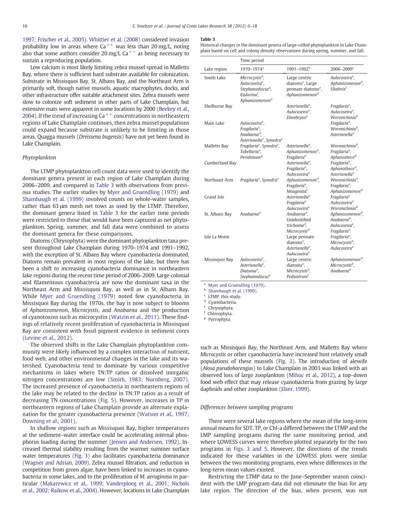
Table 3Historical changes in the dominant genera of large-celled phytoplankton in Lake Cham-plain based on cell and colony density observations during spring, summer, and fall.

Time period

Lake region 1970–1974a 1991–1992b 2006–2009c

South Lake Microcystisd,Aulocoseirae,Stephanodiscuse,Eudorinaf,Aphanizomenond

Large centricdiatomse, Largepennate diatomse,Aphanizomenond

Aulocoseirae,Aphanizomenond,Ulothrixf

Shelburne Bay Asterionellae,Aulocoseirae,Dinobryone

Fragilariae,Aulocoseirae,Woronichiniad

Main Lake Aulocoseirae,Fragilariae,Anabaenad,Asterionellae, Synedrae

Fragilariae,Woronichiniad,Asterionellae

Malletts Bay Fragilariae, Synedrae,Tabellariae,Peridiniumg

Asterionellae,Aphanizomenond,Fragilariae

Woronichiniad,Fragilariae,Aphanotheced

Cumberland Bay Asterionellae,Fragilariae,Aulocoseirae

Fragilariae,Aphanotheced,Asterionellae

Northeast Arm Fragilariae, Synedrae Aphanizomenond,Fragilariae,Mougeotiaf

Woronichiniad,Fragilariae,Aphanizomenond

Grand Isle Asterionellae Fragilariae

Fragilariae Aulocoseirae

Aulocoseirae Woronichiniad

St. Albans Bay Anabaenad Anabaenad,Unidentifiedtrichomed,Microcystisd

Aphanizomenond,Anabaenad,Aulocoseirae,Fragilariae

Isle La Motte Large pennatediatomse,Asterionellae,Aulocoseirae

Fragilariae,Microcystisd,Aulocoseirae

Missisquoi Bay Aulocoseirae,Asterionellae,Diatomae,Stephanodiscuse

Large centricdiatomse,Microcystisd,Pediastrumf

Aphanizomenond,Microcystisd,Anabaenad

a Myer and Gruendling (1979).b Shambaugh et al. (1999).c LTMP, this study.d Cyanobacteria.e Chrysophyta.f Chlorophyta.g Pyrrophyta.

16 E. Smeltzer et al. / Journal of Great Lakes Research 38 (2012) 6–18

1997; Frischer et al., 2005). Whittier et al. (2008) considered invasionprobability low in areas where Ca++ was less than 20 mg/L, notingalso that some authors consider 20 mg/L Ca++ as being necessary tosustain a reproducing population.

Low calcium is most likely limiting zebra mussel spread in MallettsBay, where there is sufficient hard substrate available for colonization.Substrate in Missisquoi Bay, St. Albans Bay, and the Northeast Arm isprimarily soft, though native mussels, aquatic macrophytes, docks, andother infrastructure offer suitable attachment sites. Zebra mussels wereslow to colonize soft sediment in other parts of Lake Champlain, butextensive mats were apparent in some locations by 2000 (Beekey et al.,2004). If the trend of increasing Ca++ concentrations in northeasternregions of Lake Champlain continues, then zebra mussel populationscould expand because substrate is unlikely to be limiting in thoseareas. Quagga mussels (Dreissena bugensis) have not yet been found inLake Champlain.

Phytoplankton

The LTMP phytoplankton cell count data were used to identify thedominant genera present in each region of Lake Champlain during2006–2009, and compared in Table 3 with observations from previ-ous studies. The earlier studies by Myer and Gruendling (1979) andShambaugh et al. (1999) involved counts on whole-water samples,rather than 63 μm mesh net tows as used by the LTMP. Therefore,the dominant genera listed in Table 3 for the earlier time periodswere restricted to those that would have been captured as net phyto-plankton. Spring, summer, and fall data were combined to assessthe dominant genera for these comparisons.

Diatoms (Chrysophyta)were the dominant phytoplankton taxa pre-sent throughout Lake Champlain during 1970–1974 and 1991–1992,with the exception of St. Albans Bay where cyanobacteria dominated.Diatoms remain prevalent in most regions of the lake, but there hasbeen a shift to increasing cyanobacteria dominance in northeasternlake regions during the recent time period of 2006–2009. Large colonialand filamentous cyanobacteria are now the dominant taxa in theNortheast Arm and Missisquoi Bay, as well as in St. Albans Bay.While Myer and Gruendling (1979) noted few cyanobacteria inMissisquoi Bay during the 1970s, the bay is now subject to bloomsof Aphanizomenon, Microcystis, and Anabaena and the productionof cyanotoxins such as microcystin (Watzin et al., 2011). These find-ings of relatively recent proliferation of cyanobacteria in MissisquoiBay are consistent with fossil pigment evidence in sediment cores(Levine et al., 2012).

The observed shifts in the Lake Champlain phytoplankton com-munity were likely influenced by a complex interaction of nutrient,food web, and other environmental changes in the lake and its wa-tershed. Cyanobacteria tend to dominate by various competitivemechanisms in lakes where TN:TP ratios or dissolved inorganicnitrogen concentrations are low (Smith, 1983; Nurnberg, 2007).The increased presence of cyanobacteria in northeastern regions ofthe lake may be related to the decline in TN:TP ratios as a result ofdecreasing TN concentrations (Fig. 5). However, increases in TP innortheastern regions of Lake Champlain provide an alternate expla-nation for the greater cyanobacteria presence (Watson et al., 1997;Downing et al., 2001).

In shallow regions such as Missisquoi Bay, higher temperaturesat the sediment–water interface could be accelerating internal phos-phorus loading during the summer (Jensen and Andersen, 1992). In-creased thermal stability resulting from the warmer summer surfacewater temperatures (Fig. 3) also facilitates cyanobacteria dominance(Wagner and Adrian, 2009). Zebra mussel filtration, and reduction incompetition from green algae, have been linked to increases in cyano-bacteria in some lakes, and to the proliferation of M. aeruginosa in par-ticular (Makarewicz et al., 1999; Vanderploeg et al., 2001; Nicholset al., 2002; Raikow et al., 2004). However, locations in Lake Champlain

such as Missisquoi Bay, the Northeast Arm, and Malletts Bay whereMicrocystis or other cyanobacteria have increased host relatively smallpopulations of these mussels (Fig. 3). The introduction of alewife(Alosa pseudoharengus) to Lake Champlain in 2003 was linked with anobserved loss of large zooplankton (Mihuc et al., 2012), a top–downfood web effect that may release cyanobacteria from grazing by largedaphnids and other zooplankton (Elser, 1999).

Differences between sampling programs

There were several lake regions where the mean of the long-termannual means for SDT, TP, or Chl-a differed between the LTMP and theLMP sampling programs during the same monitoring period, andwhere LOWESS curves were therefore plotted separately for the twoprograms in Figs. 3 and 5. However, the directions of the trendsindicated for these variables in the LOWESS plots were similarbetween the two monitoring programs, even where differences in thelong-term mean values existed.

Restricting the LTMP data to the June–September season coinci-dent with the LMP program data did not eliminate the bias for anylake region. The direction of the bias, when present, was not

17E. Smeltzer et al. / Journal of Great Lakes Research 38 (2012) 6–18

consistently positive or negative among the lake regions, which sug-gests that a difference in sampling technique between programs(Table 1) was probably not the major factor responsible for the bias.

Differences in navigation methods used by the LMP (visual land-marks) and the LTMP (electronic aids) could have led to samples beingobtained from slightly different locations within these lake regions.Strong spatial water quality gradients are known to exist in someareas of Lake Champlain, particularly in the South Lake, ShelburneBay, and St. Albans Bay, and errors in locating sampling locationsmight explain the discrepancies in the results for these areas. Pro-viding citizen monitors with navigation aids such as global position-ing system devices would be an appropriate way to eliminate thispotential problem in future monitoring programs on Lake Champlainand other large lakes.

Conclusions

The “long-term” monitoring window of 18–46 years for the datapresented here represents an extremely brief period of time relativeto the 9000 years that Lake Champlain has existed in its present geo-logic form. The fact that measureable environmental trends wereobserved during the monitoring period suggests that anthropogenicinfluences were primarily responsible. However, the changes in thelake did not always occur as predicted from trends in environmentalstressors and management activities. The spread of zebra musselshas been slower than expected in northeastern lake regions andmay be limited by low Ca++ concentrations. There was no prolifera-tion of cyanobacteria species such as M. aeruginosa that could belinked to zebra mussels, as has occurred in some of the Great Lakes.TP and Chl-a declined in some areas of the lake but not in the moreeutrophic northeastern lake regions, despite significant manage-ment efforts at controlling point and nonpoint sources in the water-shed. The lakewide decline in TN was a surprising finding, given theincreases in corn production and fertilizer use in the watershed, andmight have been due in part to regional reductions in atmosphericnitrogen deposition rates.

The scope and sometimes unexpected nature of environmentalchanges that have occurred in Lake Champlain illustrate the impor-tance of continuing the long-term monitoring programs. The aware-ness and understanding of alterations in the lake's ecosystem gainedfrom monitoring can be used to direct management responses in amore timely and effective manner. Lake Champlain experienced his-torically unprecedented flooding during the spring of 2011, followedby destructive river flows from Tropical Storm Irene in August, 2011.The data provided by the ongoing monitoring programs will beinvaluable in assessing the environmental effects of these extremeweather events.

This paper presents only a limited subset of the variables andmonitoring sites encompassed in the current monitoring databases,and numerous research questions remain. The authors hope that theavailability of the Long-Term Monitoring Program dataset on the in-ternet may stimulate further analyses and investigation of ecologicalchanges in Lake Champlain.

Acknowledgments

The LTMP has been supported by the Lake Champlain Basin Pro-gram and by the States of Vermont and New York. We thank themany staff of the Vermont DEC and the New York State DEC who pro-vided field assistance and laboratory analyses in support of the LTMPover the years, and all past and present LMP program coordinatorsand volunteers for making that long-term dataset possible. We thankJ.E. Marsden and two anonymous reviewers for comments that im-proved the manuscript.

References

Austin, J.A., Colman, S.M., 2007. Lake Superior summer water temperatures are increasingmore rapidly than regional air temperatures: a positive ice-albedo feedback. Geophys.Res. Lett. 34, L06604. doi:10.1029/2006GL029021.

Barbiero, R.P., Tuchman, M.L., 2004. Long-term dreissenid impacts on water clarity inLake Erie. J. Great Lakes Res. 30 (4), 557–565.

Barbiero, R.P., Tuchman, M.L., Millard, E.S., 2006. Post-dreissenid increases in trans-parency during summer stratification in the offshore waters of Lake Ontario: isa reduction in whiting events the cause? J Great Lakes Res. 32 (1), 131–141.

Beekey,M.A.,McCabe, D.J., Marsden, J.E., 2004. Zebramussel colonisation of soft sedimentsfacilitates invertebrate communities. Freshw. Biol. 49, 535–545.

Bogdan, K.G., 1978. Estimates of the annual loading of total phosphorus to Lake Champlain.Prep. for the Eutrophication Task Force, Lake Champlain Basin Study. New EnglandRiver Basins Commission, Burlington, VT.

Burns, N.M., Rockwell, D.C., Bertram, P.E., Dolan, D.M., Ciborowski, J.J.H., 2005.Trends in temperature, Secchi depth, and dissolved oxygen depletion rates inthe Central Basin of Lake Erie, 1983–2002. J. Great Lakes Res. 31 (Supplement 2),35–49.

Canfield Jr., D.E., Brown, C.D., Bachmann, R.W., Hoyer, M.V., 2002. Volunteer lakemonitoring: testing the reliability of data collected by the Florida LAKEWATCHProgram. Lake Reserv. Manage. 18 (1), 1–9.

Chapra, S.C., Dove, A., Rockwell, D.C., 2009. Great Lakes chloride trends: long-termmass balance and loading analysis. J. Great Lakes Res. 35 (2), 272–284.

Cohn, A.B., Manley, T.O., Manley, P.L., Smeltzer, E., Watzin, M.C., 2007. Lake Champlain:research and management in the presence of history. LakeLine 27 (4), 46–56 NorthAmerican Lake Management Society. Madison, WI.

Daley, M.L., Potter, J.D., McDowell, W.H., 2009. Salinization of urbanizing New Hampshirestreams and groundwater: effects of road salt and hydrologic variability. J. N. Am.Benthol.l Soc. 28 (4), 929–940.

Denner, J.C., Clark Jr., S.F., Smith, T.E., Medalie, L., 2010. Effects of highway road saltingon the water quality of selected streams in Chittenden County, Vermont, November2005–2007. U.S. Geological Survey Scientific Investigations Report 2009–5236. 43 p.

Dobiesz, N.E., Lester, N.P., 2009. Changes in mid-summer water temperature and clarityacross the Great Lakes between 1968 and 2002. J. Great Lakes Res. 35 (3), 371–384.

Downing, J.A., Watson, S.B., McCauley, E., 2001. Predicting cyanobacteria dominance inlakes. Can. J. Fish. Aquat. Sci. 58 (10), 1905–1908.

Effler, S.W., Perkins, M., Johnson, D.L., 1991. Optical heterogeneity in Lake Champlain.J. Great Lakes Res. 17 (3), 322–332.

Eimers, M.C., Winter, J.G., Scheider, W.A., Watmough, S.A., Nicholls, K.H., 2005. Recentchanges and patterns in the water chemistry of Lake Simcoe. J. Great Lakes Res. 31(3), 322–332.

Elser, J.J., 1999. The pathway to noxious cyanobacteria blooms in lakes: the food web asthe final turn. Freshw. Biol. 42, 537–543.

Elser, J.J., Andersen, T., Baron, J.S., Bergstrom, A.K., Jansson, M., Kyle, M., Nydick, K.R.,Steger, L., Hessen, D.O., 2009. Shifts in lake N:P stoichiometry and nutrient limita-tion driven by atmospheric nitrogen deposition. Science 326, 835–837.

Eyles, N., Meriano, M., 2010. Road-impacted sediment and water in a Lake Ontariowatershed and lagoon, City of Pickering, Ontario, Canada: an example of urbanbasin analysis. Sediment. Geol. 224 (1), 15–28.

Fahnenstiel, G., Nalepa, T., Pothoven, S., Carrick, H., Scavia, D., 2010. Lake Michiganlower food web: long-term observations and Dreissena impact. J. Great Lakes Res.36 (Supplement 3), 1–4.

Frischer, M.E., McGrath, B.R., Hansen, A.S., Vescio, P.A., Wyllie, J.A., Wimbush, J., Nierzwicki-Bauer, S.A., 2005. Introduction pathways, differential survival of adult and larval zebramussels (Dreissena polymorpha), and possible management strategies, in anAdirondack Lake, Lake George, NY. Lake Reserv. Manage. 21 (4), 391–402.

Hampton, S.E., Izmesteva, L.R., Moore, M.V., Katz, S.L., Dennis, B., Silow, E., 2008. Sixtyyears of environmental change in the world's largest freshwater lake—Lake Baikal,Siberia. Global Change Biol. 14 (8), 1947–1958.

Helsel, D.R., Hirsch, R.M., 2005. Statistical methods in water resources. U.S. GeologicalSurvey, Techniques of Water Resources Investigations, Book 4, Chapter A3.

Henson, E.B., Potash, M., 1966. A synoptic survey of Lake Champlain, summer 1965.Univ. Michigan Great Lakes Res. Div. Publ. No. 15, pp. 38–43.

Henson, E.B., Potash, M., 1987. Sampling strategies for detecting water qualitytrends in Lake Champlain. Completion Report to the U.S. Dept. Interior Officeof Water Resources and Technology. Project No. 03. University of Vermont,Burlington.

Higgins, S.N., Vander Zanden, M.J., 2010. What a difference a species makes: a meta-analysis of dreissinid mussel impacts on freshwater ecosystems. Ecol. Monogr. 80(2), 179–196.

Hincks, S.S., Mackie, G.L., 1997. Effects of pH, calcium, alkalinity, hardness, and chloro-phyll on the survival, growth, and reproductive success of zebra mussel (Dreissenapolymorpha) in Ontario lakes. Can. J. Fish. Aquat. Sci. 54 (9), 2049–2057.

Jankowski, T., Livingstone, D.M., Buhrer, H., Forster, R., Niederhauser, P., 2006. Conse-quences of the 2003 European heat wave for lake temperature profiles, thermalstability, and hypolimnetic oxygen depletion: implications for a warmer world.Limnol. Oceanogr. 51 (2), 815–819.

Jensen, H.S., Andersen, F.O., 1992. Importance of temperature, nitrate, and pH for phos-phate release from aerobic sediments of four shallow, eutrophic lakes. Limnol.Oceanogr. 37 (3), 577–589.

Kauschal, S.S., Groffman, P.M., Likens, G.E., Belt, K.T., Stack, W.P., Kelly, V.R., Band, L.E.,Fisher, G.T., 2005. Increased salinization of fresh water in the northeastern UnitedStates. Proc. Nat. Acad. Sci. 102 (38), 13517–13520.

Langen, T.A., Twiss, M., Young, T., Janoyan, K., Stager, J.C., Osso Jr., J., Prutzman, H.,Green, B., 2006. Environmental impacts of winter road management at the Cascade

18 E. Smeltzer et al. / Journal of Great Lakes Research 38 (2012) 6–18

Lakes and Chapel Pond. Clarkson Center for the Environment. Report 1. ClarksonUniversity, Potsdam, NY.

Levine, S.N., Lini, A., Ostrofsky, M.L., Bunting, L., Burgess, H., Leavitt, P.R., Reuter, D.,Lami, A., Guilizzoni, P., 2012. The eutrophication of Lake Champlain's NortheastArm: insights from paleolimnological analyses. J. Great Lakes Res. 38 (Supplement 1),35–48.

Lovett, G.M., Burns, D.A., Driscoll, C.T., Jenkins, J.C., Mitchell, M.J., Rustad, L., Shanley, J.B.,Likens, G.E., Haeuber, R., 2007. Who needs environmental monitoring? Front. Ecol.Environ. 5 (5), 253–260.

MACTEC Engineering and Consulting, Inc., 2010. Clean Air Status and Trends Network(CASTNET) 2008 annual report. Prep. for U.S. Environmental Protection Agency.Washington, D.C.

Makarewicz, J.C., Lewis, T.W., Bertram, P., 1999. Phytoplankton composition and bio-mass in the offshore waters of Lake Erie: pre- and post-Dreissena introduction(1983–1993). J. Great Lakes Res. 25 (1), 135–148.

Manley, T.O., Hunkins, K.L., Saylor, J.H., Miller, G.S., Manley, P.L., 1999. Aspects ofsummertime and wintertime hydrodynamics of Lake Champlain. In: Manley, T.O.,Manley, P.L. (Eds.), Lake Champlain in Transition: FromResearch Toward Restoration:American Geophysical Union. Water Sci. Appl., 1, pp. 67–115. Washington, D.C.

Marsden, J.E., 1992. Standard protocols for monitoring and sampling zebra mussels.Illinois Natural History Survey Biological Notes 138. Champaign, IL.

Marsden, J.E., Hauser, M., 2009. Exotic species in Lake Champlain. J. Great Lakes Res. 35(2), 250–265.

Matthews, D.A., Effler, S.W., 2006. Assessment of long-term trends in the oxygen resourcesof a recovering urban lake, Onondaga Lake, NY. Lake Reserv. Manage. 22 (1), 19–32.

McDonald, C.P., Urban, N.R., Casey, C.M., 2010. Modeling historical trends in LakeSuperior total nitrogen concentrations. J. Great Lakes Res. 36, 715–721.

Medalie, L., Smeltzer, E., 2004. Status and trends of phosphorus in Lake Champlain andits tributaries, 1990–2000. In: Manley, T., et al. (Ed.), Lake Champlain: Partnershipand Research in the New Millennium. Kluwer Academic/Plenum Publishers, NewYork, pp. 191–219.

Medalie, L., Hirsch, R.M., Archfield, S.A., 2012. Use of flow-normalization to evaluatenutrient concentration and flux changes in Lake Champlain tributaries, 1990–2009.J. Great Lakes Res. 38 (Supplement 1), 58–67.

Mellina, E., Rasmussen, J.B., 1994. Patterns in the distribution and abundance of zebramussel (Dreissena polymorpha) in rivers and lakes in relation to substrate andother physicochemical factors. Can. J. Fish. Aquat. Sci. 51 (5), 1024–1036.

Mida, J.L., Scavia, D., Fahnenstiel, G.L., Pothoven, S.A., Vanderploeg, H.A., Dolan, D.M.,2010. Long-term and recent changes in southern Lake Michigan water quality withimplications for present trophic status. J. Great Lakes Res. 36 (Supplement 3), 42–49.

Mihuc, T.B., Dunlap, F., Binggeli, C., Pershyn, C., Myers, L., Groves, A., Waring, A., 2012.Long-term patterns in Lake Champlain's zooplankton: 1992–2010. J. Great LakesRes. 38 (Supplement 1), 49–57.

Mullaney, J.R., Lorenz, D.L., Arntson, A.D., 2009. Chloride in groundwater and surfacewater in areas underlain by the glacial aquifer system, northern United States.U.S. Geological Survey Scientific Investigations Report 2009–5086. 41 p.

Myer, G.E., Gruendling, G.K., 1979. Limnology of Lake Champlain. Prep. for New EnglandRiver Basins Commission. Burlington, VT.

Nichols, K.K., Heintsch, L., Carney, E., 2002. Univariate step-trend andmulti-variate assess-ments of the apparent effects of P loading reductions and zebra mussels on the phy-toplankton of the bay in Quinte, Lake Ontario. J. Great Lakes Res. 28 (1), 15–31.

Novotny, E.V., Stefan, H.G., 2009. Projections of chloride concentrations in urban lakesreceiving road de-icing salt. Water Air Soil Pollut. doi:10.1007/s11270-009-0297-0.

Nurnberg, G.K., 2007. Low-nitrate-days (LND), a potential indicator of cyanobacteriablooms in a eutrophic hardwater reservoir. Water Qual. Res. J. Can. 42 (4), 269–283.

Picotte, A., Pomeroy, S., 2000. Vermont Lay Monitoring Manual. Vermont Agency ofNatural Resources, Waterbury, VT.

Potash, M., Henson, E.B., 1975. Chemical changes in Lake Champlain: a decade of obser-vations. Verh. Internat. Verein. Limnol. 19, 421–428.

Potash, M., Sundberg, S.E., Henson, E.B., 1969. Characterization of water masses ofLake Champlain. Verh. Internat. Verein. Limnol. 17, 140–147.

Raikow, D.F., Sarnelle, O., Wilson, A.E., Hamilton, S.K., 2004. Dominance of the noxiouscyanobacterium Microcystis aeruginosa in low-nutrient lakes is associated withexotic zebra mussels. Limnol. Oceanogr. 49 (2), 482–487.

Robinson, K.W., Campbell, J.P., Jaworski, N.A., 2003. Water-quality trends in New Englandrivers during the 20th century. U.S. Geological SurveyWater Resources InvestigationsReport 03–4012.

Rockwell, D.C., Warren, G.J., Bertram, P.E., Salisbury, D.K., Burns, N.M., 2005. The U.S.EPA Lake Erie indicators monitoring program 1983–2002: trends in phosphorus,silica, and chlorophyll a in the Central Basin. J. Great Lakes Res. 31 (Suppl. 2), 23–34.

Schindler, D.W., 2009. Lakes as sentinels and integrators for the effects of climatechange on watersheds, airsheds, and landscapes. Limnol. Oceanogr. 54, 2349–2358(6, part 2).

Shambaugh, A.D., Duchovnay, A., McIntosh, A., 1999. A survey of Lake Champlain'splankton. In: Manley, T.O., Manley, P.L. (Eds.), Lake Champlain in Transition:from research toward restoration: American Geophysical Union. Water Sci. Appl.,1, pp. 323–340. Washington, D.C.

Smeltzer, E., Quinn, S., 1996. A phosphorus budget, model, and load reduction strategyfor Lake Champlain. Lake Reserv. Manage. 12 (3), 381–393.

Smeltzer, E., Dunlap, F., Simoneau, M., 2009. Lake Champlain phosphorus concentra-tions and loading rates, 1990–2008. Lake Champlain Basin Program Tech. Rep.57. Grand Isle, VT.

Smith, V.H., 1983. Low nitrogen to phosphorus ratios favor dominance by blue-greenalgae in lake phytoplankton. Science 221, 669–671.

Stager, J.C., Thill, M., 2010. Climate change in the Lake Champlain Basin: what naturalresource managers can expect and do. Prep. for The Nature Conservancy. KeeneValley, NY and Montpelier, VT.

Stangel, P., Shambaugh, A., 2005. Lake Champlain 2004 zebra mussel monitoring pro-gram. Final Report. Vermont Dept. Environ. Conserv, Waterbury, VT.

Trowbridge, P.R., Sassan, D., Heath, D.L., Walsh, E.M., 2010. Relating road salt to excee-dances of the water quality standard for chloride in New Hampshire Streams.Environ. Sci. Technol. 44 (13), 4903–4909.

Troy, A., Wang, D., Capen, D., 2007. Updating the Lake Champlain Basin land use data toimprove prediction of phosphorus loading. Lake Champlain Basin Program Tech.Rep, 54. Grand Isle, VT.

U.S. Environmental Protection Agency, 1988. Ambient Water Quality Criteria for Chloride—1988. Office of Water, Washington D.C. EPA 440/5-88-001.

Vanderploeg, H.A., Liebig, J.R., Carmichael, W.W., Agy, M.A., Johengen, T.H., Fahnenstiel,G.L., Nalepa, T.F., 2001. Zebra mussel (Dreissena polymorpha) selective filtrationpromoted toxic Microcystis blooms in Saginaw Bay (Lake Huron) and Lake Erie.Can. J. Fish. Aquat. Sci. 58 (6), 1208–1221.

Vermont Agency of Natural Resources and Vermont Agency of Agriculture, Food andMarkets, 2010. Vermont clean and clear action plan 2009 annual report. Submittedto the Vermont General Assembly. Montpelier, VT.

Vermont Department of Environmental Conservation and New York State Departmentof Environmental Conservation, 1997. A phosphorus budget, model, and load re-duction strategy for Lake Champlain. Lake Champlain Diagnostic-FeasibilityStudy Final Report. . Waterbury, VT and Albany, NY.

Vermont Department of Environmental Conservation and New York State Departmentof Environmental Conservation, 2010. Long-term water quality and biologicalmonitoring project for Lake Champlain. Quality Assurance Project Plan. : Prep. forLake Champlain Basin Program. Grand Isle, VT.

Wagner, C., Adrian, R., 2009. Cyanobacteria dominance: quantifying the effects of cli-mate change. Limnol. Oceanogr. 54, 2460–2468 (6, part 2).

Watson, S.B., McCauley, E., Downing, J.A., 1997. Patterns in phytoplankton taxonomiccomposition across temperate lakes of differing nutrient status. Limnol. Oceanogr.42 (3), 487–495.

Watzin, M.C., 2007. The promise of adaptive management. In: Schepf, M., Cox, C. (Eds.),Managing agricultural landscapes for environmental quality: strengthening thescience base. Soil and Water Conservation Society Press, Ankeny, IA, pp. 147–158.

Watzin, M., Fuller, S., Bronson, L., Gorney, R., Shuster, L., 2011. Monitoring and evalua-tion of cyanobacteria in Lake Champlain, summer 2009. Lake Champlain Basin Pro-gram Tech. Rep. No. 61. Grand Isle, VT.

Wetzel, R.G., Likens, G.E., 2000. Limnological Analyses, 3rd ed. Springer-Verlag, NewYork. 429 pp.

Whittier, T.R., Ringold, P.L., Herlihy, A.T., Pierson, S.M., 2008. A calcium-based invasionrisk assessment for zebra and quagga mussels (Dreissena spp.). Front. Ecol. Environ.(6). doi:10.1890/070073.

Journal of Great Lakes Research 38 (2012) 1–5

Contents lists available at SciVerse ScienceDirect

Journal of Great Lakes Research

j ourna l homepage: www.e lsev ie r .com/ locate / jg l r

Lake Champlain 2010: A summary of recent research and monitoring initiatives

Douglas E. Facey a,⁎, J. Ellen Marsden b,1, Timothy B. Mihuc c,2, Eric A. Howe d,3

a 302B Cheray Science Hall, Saint Michael's College, Colchester, VT 05439, USAb Rubenstein School of Environment and Natural Resources, Aiken Center, 81 Carrigan Dr., University of Vermont, Burlington, VT 05405, USAc Lake Champlain Research Institute, SUNY Plattsburgh, Plattsburgh, NY 12901, USAd Lake Champlain Basin Program, 54 West Shore Rd., Grand Isle, VT, USA 05458

⁎ Corresponding author. Tel.: +1 802 654 2625.E-mail addresses: dfacey@smcvt.edu (D.E. Facey), el

(J.E. Marsden), mihuctb@plattsburgh.edu (T.B. Mihuc),1 Tel.: +1 802 656 0684; fax: +1 802 656 8683.2 Tel.: +1 518 564 3039; fax: +1 518 564 5267.3 Tel.: +1 802 372 3213; fax: +1 802 372 3233.

0380-1330/$ – see front matter © 2011 International Adoi:10.1016/j.jglr.2011.12.001

a b s t r a c t

a r t i c l e i n f o

Article history:Received 24 October 2011Accepted 1 December 2011Available online 31 December 2011

Communicated by Joseph C. Makarewicz

Index words:ManagementHydrodynamicsHistoryRecreationFisheriesCormorants

Lake Champlain shares a geological history with the Great Lakes and, as part of the St. Lawrence drainage, alsoshares biological and ecological similarities. The complex bathymetry and extensive shoreline provide a varietyof lacustrine habitats, fromdeep oligotrophic areas to shallowbays that are highly eutrophic. The large basin:lakeratio (19:1)makes Lake Champlain vulnerable to impacts associatedwith land use, and in some parts of the lakethese impacts are further exacerbated by limited water exchange among lake segments due to both natural andanthropogenic barriers. Research in Lake Champlain and the surrounding basin has expanded considerably sincethe 1970s, with a particularly dramatic increase since the early 1990s. This special issue of the Journal of GreatLakes Research brings together 16 reports from recent research and monitoring efforts in Lake Champlain. Thepapers cover a variety of topics but primarily focus on lake hydrodynamics; historical and recent chemicalchanges in the lake; phosphorus loading; recent changes in populations of phytoplankton, zooplankton, and fish-es; impacts of invasive species; recreational use; and the challenges of management decision-making in a lakethat falls within the legal jurisdictions of two U.S. states, one Canadian province, two national governments,and the International Joint Commission. The papers provide not only evaluations of progress on some criticalmanagement issues but also valuable reference points for future research.

© 2011 International Association for Great Lakes Research. Published by Elsevier B.V. All rights reserved.

Introduction

After the last ice age drew to a close and the Laurentide ice sheetretreated northward, for a period of about 1500 years water from theGreat Lakes region drained throughwhat is now the Lake Champlain val-ley on its way to the Atlantic Ocean. As a result, the Great Lakes and LakeChamplain share a geological history and biological and ecological simi-larities. Lake Champlain is much smaller and shallower and has a shortretention time relative to theGreat Lakes. In contrast, the Lake Champlaindrainage basin is quite large compared to the lake area (a 19:1 ratio);11 major rivers (32–102 km) and many smaller streams drain theGreen Mountains to the east and the Adirondack Mountains to thewest. Consequently, the lake is highly vulnerable to severe precipitationevents, snowmelt conditions, and human alterations of the landscape. Asevidence of this, the water level normally fluctuates 1–2 m in a year; inthe historic spring flood of 2011, the lake level rose to 103.3′ above sealevel (31.5 m), 1 m above the flood stage of 30.5 m, and over 2 mabove the mean lake level (29.1 m).

len.marsden@uvm.eduehowe@lcbp.org (E.A. Howe).

ssociation for Great Lakes Research.

Lake Champlain has a complex bathymetry, with over 70 islands, ashoreline of over 800 km (Myer and Gruendling, 1979), and manysemi-isolated bays and inlets. The lake is divided into fivemajor lake ba-sins created by natural and anthropogenic barriers: the South Lake, theMain Lake, the Northeast Arm,Malletts Bay, andMissisquoi Bay (Fig. 1).The South Lake is shallow (b7 m), narrow (averagewidth 1 km),warm,eutrophic, and essentially riverine. Water flows northward through anarrow constriction at Crown Point into the Main Lake, which extendsnorthward to the Canadian border and drains, via the Richelieu River,into the St. Lawrence River near Montreal. The Main Lake, which is oli-gotrophic to mesotrophic, extends from the Crown Point bridge northto Rouses Point, New York, at the Canadian border and contains over80% of the total lake volume, including almost 60% of the surface areaand the deepest portion of the lake (122 m) (Myer and Gruendling,1979). The Alburg peninsula, two large islands, and a series of cause-ways separate the northern Main Lake to the west from three smallerbasins to the east. The southernmost of these basins is Malletts Bay,which is moderately deep (maximum depth 30 m) and mesotrophic.Water from Malletts Bay flows west into the Main Lake through twonarrow gaps in an old railroad causeway, and north through a gap in asecond causeway into the Northeast Arm, also known locally as the In-land Sea. Historically, the Northeast Arm was partially isolated fromMalletts Bay by a shallow sandbar resulting from sediments depositedby the Lamoille River; a highway causeway with a single narrow open-ing now crosses that sandbar. The Northeast Arm is moderately deep

Published by Elsevier B.V. All rights reserved.

Fig. 1. Map of Lake Champlain showing the five basins.

2 D.E. Facey et al. / Journal of Great Lakes Research 38 (2012) 1–5

(maximum 50m) and oligotrophic to mesotrophic. To the north of theNortheast Arm is Missisquoi Bay, a shallow (4.3 m), warm, now eutro-phic bay that spans the Vermont–Quebec border. The natural narrowopening between the Northeast Arm and Missisquoi Bay was furtherconstricted by a highway causeway, which was replaced by a bridgein 2003. As a result of its bathymetric profile – long, narrow, with adeep ravine – the lake has a complex hydrological dynamic involvinglong-term and short-term seiches and substantial currents (Manley,2004; Manley et al., 1999b, 2012b).

Management and research background

Similar to the Great Lakes, management and policy decisions regard-ing Lake Champlain are made all the more challenging by the fact thatmultiple legal entities have jurisdiction over different parts of the lakeand the basin. In Lake Champlain, as many as six jurisdictional entitiesmay weigh in on some issues — the states of New York and Vermont,the province of Quebec, the U.S. and Canadian federal governments,and the International Joint Commission. Québec, NewYork, and Vermonthave a formal memorandum of understanding on cooperation of envi-ronmental management of Lake Champlain. The Lake Champlain SpecialDesignation Act created the Lake Champlain Basin Program (LCBP) in1990 with the goal of coordinating and funding efforts which benefitthe Lake Champlain basin's water quality, fisheries, wetlands, wildlife,recreation, and cultural resources. Among the challenges faced by theLCBP has been negotiating positions among the six legal jurisdictions.In this special issue, Wroth (2012) reviews the historical legacies of thesix managing jurisdictions and offers insight into potential ways to fur-ther facilitate solutions to the issues confronting those agencies withthe responsibility of addressing the multiple environmental challengesof the Lake Champlain basin.

Many agencies have conductedmonitoring and research programsin the watershed. The first major biological survey of Lake Champlainwas conducted in the early 1900s by the New York State ConservationDepartment (Moore, 1930). Extensive work on lake habitat, hydrody-namics, chemistry, and the lower food web was conducted in the1960s and 1970s by Henson and Potash (1970) and Myer andGruendling (1979). Subsequent fisheries surveys were conducted byboth states (reviewed by Marsden and Langdon, 2012).

In 1991 the newly formed Lake Champlain Research Consortium(LCRC) brought together seven academic institutions in the Lake Cham-plain basin to coordinate and facilitate research on Lake Champlain. TheLCBP and LCRC have cooperatively and independently organized and fa-cilitated several small research conferences, and larger conferences in1998, 2002, and 2008; papers from the first two conferences were pub-lished in special volumes (Manley and Manley, 1999; Manley et al.,2004; http://academics.smcvt.edu/lcrc/). In 2010, the LCRC and LCBPco-hosted a research conference that brought together a range of re-search presentations focusing on Lake Champlain and its watershed(http://academics.smcvt.edu/lcrc/); many of the papers published inthis special issue of the Journal of Great Lakes Research are based on re-search presented at that conference.

Hydrodynamics

The complexphysical structure of LakeChamplain presents challengesfor understanding the lake's hydrodynamic patterns. New York's Adiron-dack Mountains to the west and Vermont's Green Mountains to the eastchannel winds through the Champlain Valley, such that prevailingwinds are from the south or north.Winds produce internal seiche activityin the Main Lake that extends as far as the South Lake and create circularcurrents along thewestern and eastern sides of the lake (Manley, 2004). Acloser study of these circular patterns from 2002 to 2004 byManley et al.(2012b) in this issue revealed three main circulation systems: (1) off-shore, both the epilimnion and hypolimnion showed circular to ellipticalmotions; (2) nearshore currents created linear to curvilinear motions;and (3) southerly winds generated a strong westerly subsurface flow(10–16 m) and a strong southerly flownear thewestern shore. Thewest-ern subsurface flow seems to be driven by upwelling of hypolimneticwater along some parts of the shoreline. Northerly winds may create anopposite circulation pattern, with easterly subsurface flows and a north-erly current along the east shore (Manley et al., 2012b).

The benthic currents created by the seiche activity are capable of dis-placing sediments, thereby creating areas of erosion anddepositionbasedon benthic topography. Benthic sedimentary furrows oriented along thelong axis of Lake Champlain are a result of the redistribution of sedimentsby seiche-driven bottom currents (Manley et al., 1999a). In more recentwork presented in this issue, high-resolution seismic profiles in a deepsection of theMain Lake show two lacustrine sediment drifts, and subse-quent dating of sediment core reveal that these began developing about8700–8800 years ago (Manley et al., 2012a).

Chemical and biological characteristics

The large size of Lake Champlain's watershed, relative to lake volume,makes the lake vulnerable to land-use changes such as deforestation, in-creasing use of manure and fertilizer in agriculture, wastewater inputs,and industrial effluent. Monitoring of several fundamental physical andchemical parameters of Lake Champlain was conducted in the 1960s,but a more intensive and regular long-term monitoring program beganin 1992, conducted jointly by the Vermont and New York Departmentsof Environmental Conservation in collaboration with the LCBP. In thisissue, Smeltzer et al. (2012) evaluate data from this long-term monitor-ing effort to assess changes in physical and chemical attributes of thelake. For example, summer water clarity in the Main Lake increased byover a meter between 1964 and 2009. Most of this increase occurredafter 1993, the year that zebra mussels (Dreissena polymorpha) became

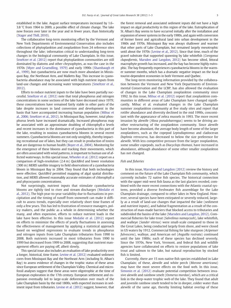
3D.E. Facey et al. / Journal of Great Lakes Research 38 (2012) 1–5

established in the lake. August surface temperatures increased by 1.6–3.8 °C from 1964 to 2009, a possible effect of climate change. The lakenow freezes over later in the year and in fewer years, than historically(Stager and Thill, 2010).

The collaborative long-term monitoring effort by the Vermont andNew York Departments of Environmental Conservation also includescollections of phytoplankton and zooplankton from 24 reference sitesthroughout the lake; information critical to understanding long-termchanges in the biological community of Lake Champlain. In this issue,Smeltzer et al. (2012) report that phytoplankton communities are stilldominated by diatoms and other chrysophytes, as was the case in the1970s (Myer and Gruendling, 1979) and early 1990s (Shambaugh etal., 1999), but cyanobacteria are now much more abundant in Missis-quoi Bay, the Northeast Arm, and Malletts Bay. This increase in cyano-bacteria abundance may be associated with high nutrient inputs fromland-use changes and increasing water temperatures (Smeltzer et al.,2012).

Efforts to reduce nutrient inputs to the lake have been partially suc-cessful. Smeltzer et al. (2012) note that total phosphorus and nitrogenconcentrations in some sections of the lake have decreased since 1979;these concentrations have remained fairly stable in other parts of thelake despite increases in land conversion and development in thebasin that have accompanied increasing human population (Mihuc etal., 2006; Smeltzer et al., 2012). In Missisquoi Bay, however, total phos-phorus levels have increased dramatically. Increased phosphorus maybe associated with an approximate doubling of chlorophyll-a levelsand recent increases in the dominance of cyanobacteria in this part ofthe lake, resulting in noxious cyanobacteria blooms in several recentsummers. Cyanobacteria blooms are not only unsightly, thereby impact-ing recreational use of lakes, but they can result in production of toxinsthat are dangerous to human health (Boyer et al., 2004). Monitoring forthe emergence of these blooms and tracking their movements, whichare often associatedwithwind patterns, is important to humanuse of af-fected waterways. In this special issue, Wheeler et al. (2012) report on acomparison of high-resolution (2.4 m) QuickBird and lower resolution(300 m)MERIS satellite imagery to field observations of a cyanobacteriabloom in Missisquoi Bay in 2004. They found that both technologieswere effective; QuickBird permitted mapping of algal spatial distribu-tion, and MERIS allowed reasonably accurate estimates of chlorophyll aand phycocyanin concentrations.

Not surprisingly, nutrient inputs that stimulate cyanobacteriablooms are tightly tied to river and stream discharges (Medalie etal., 2012). The high year-to-year variability due to fluctuations in pre-cipitation and the timing of runoff from snowmelt can make it diffi-cult to assess trends, especially over relatively short time frames ofonly a few years. This has led to frustration of resource managers, pol-icy makers, and the public as a whole in determining whether themany, and often expensive, efforts to reduce nutrient loads in thelake have been effective. In this issue Medalie et al. (2012) reporton efforts to minimize the effects of yearly fluctuations in assessingthe effectiveness of management by applying a statistical approachbased on weighted regressions to evaluate trends in phosphorusand nitrogen inputs from Lake Champlain tributaries from 1990 to2008. Both nutrients increased in most tributaries from 1990 to1999 but decreased from 1999 to 2008, suggesting that nutrient man-agement efforts are paying off, albeit slowly.

This special issue also includes an evaluation of lake productivity overa longer, historical, time frame. Levine et al. (2012) evaluated sedimentcores from Missisquoi Bay and the Northeast Arm (including St. Alban'sBay) to assess evidence of changes in the trophic status of these areassince European settlement of the Champlain Valley. Chemical andmicro-fossil analyses suggest that these areas were oligotrophic at the time ofEuropean exploration in the 17th century. European settlement and ex-pansion eventually led to large-scale deforestation over much of theLake Champlain basin by the mid 1800s, with expected increases in sed-iment input from tributaries. Levine et al. (2012) suggest, however, that

the forest removal and associated sediment inputs did not have a highimpact on algal productivity in this region of the lake. Eutrophication ofSt. Alban's Bay seems to have occurred initially after the installation andexpansion of sewer systems in the early 1900s, and againwith conversionof former forest and agricultural land into urban development in the1960s and 1970s. Missisquoi Bay was always shallower and warmerthat other parts of Lake Champlain, but remained largely mesotrophicuntil about the 1970s (Levine et al., 2012). Since that time, much of thegravel substrate that supported spawning by lake whitefish (Coregonusclupeaformis, Marsden and Langdon, 2012) has become silted, littoralmacrophyte growth has increased, and the bay has become highly eutro-phic. The bay frequently experiences cyanobacteria blooms in the warm-er summer months, which has a dramatic negative impact on the localtourist-dependent economies in both Vermont and Quebec.

The long-term monitoring information provided by the collabora-tion between the Vermont and New York Departments of Environ-mental Conservation and the LCBP, has also allowed the evaluationof changes in the Lake Champlain zooplankton community since1992. In this issue, Mihuc et al. (2012) report that zooplankton com-munities in different areas of Lake Champlain have changed signifi-cantly. Mihuc et al. evaluated changes in the Lake Champlainsummer zooplankton community at five study sites and report thatrotifer abundance and diversity declined in the mid 1990s, concomi-tant with the appearance of zebra mussels in 1993. The more recentinvasion by alewife (Alosa pseudoharengus) seems to be driving an-other restructuring of the zooplankton community. Since alewifehave become abundant, the average body length of some of the largerzooplankters, such as the copepod Leptodiaptomus and cladoceranDaphnia retrocurva, has decreased to below the size preference foralewife. With less competitive pressure from the larger zooplankton,some smaller copepods, such as Diacyclops thomasi, have increased inabundance, although abundance of some other smaller zooplanktonhas not changed.

Fish and fisheries

In this issue, Marsden and Langdon (2012) review the history andcomment on the future of the Lake Champlain fish community, whichcurrently includes 72 native fish species. The historical connectionwith the upper mid-west fish fauna as the last glaciers receded, com-bined with the more recent connections with the Atlantic coastal sys-tems, provided a diverse freshwater fish assemblage for the LakeChamplain drainage, compared to other lakes in New England. How-ever, several species have been extirpated or severely reduced, large-ly as a result of land-use changes that impacted the lake (sedimentand nutrient inputs), and habitat fragmentation as a result of the con-struction of man-made barriers that blocked access to tributaries andsubdivided the basins of the lake (Marsden and Langdon, 2012). Com-mercial fisheries for lake trout (Salvelinus namaycush), lake whitefish,and walleye (Sander vitreus) were small-scale compared to those inthe Great Lakes, being conducted largely from shore, and were closedin US waters by 1912. Commercial fishing for lake sturgeon (Acipenserfulvescens), walleye, and American eel (Anguilla rostrata) continueduntil the late 1900s; each of these species has declined severely.Since the 1970s, New York, Vermont, and federal fish and wildlifeagencies have collaborated on efforts to restore populations of laketrout and salmon to the lake, but natural reproduction by stockedfish is limited.

Currently, there are 15 non-native fish species established in LakeChamplain; of these, alewife and white perch (Morone americana)may have the most severe effects on the food web. In this issue,Simonin et al. (2012) evaluate potential competition between inva-sive alewife and rainbow smelt (Osmerus mordax), which are a criticallink in the deep-water trophic web of the lake. They found that adultand juvenile rainbow smelt tended to be in deeper, colder water thanalewife of the same age, thereby limiting habitat overlap of these

4 D.E. Facey et al. / Journal of Great Lakes Research 38 (2012) 1–5

fishes within the lake. There was, however, some overlap betweenthe upper/warmer limit of the rainbow smelt range and the deeper/cooler limits of the alewife range.

Managing nuisance species

There are currently 48 non-native species in Lake Champlain, in-cluding fishes. Several of these species have reached nuisance status(Marsden and Hauser, 2009) and are the focus of management effortsto control their populations. The nuisance species that presents thegreatest management challenge is the sea lamprey (Petromyzon mar-inus) which, in contrast to its status in the upper Great Lakes, is likelynative to Lake Champlain. Anthropogenic changes in the watershedand to fish communities appear to have altered the balance of sealamprey and their prey in the Lake Champlain ecosystem (Marsdenand Langdon, 2012). In consequence, sea lamprey control hasemerged as one of the top fishery-related management issues inLake Champlain. An experimental sea lamprey control programfrom 1990 to 1998 reduced the incidence of lamprey wounding onsalmonids, and a long-term control program began in 2002. The pri-mary means of control have been chemicals that target the filter-feeding larvae, but there is ongoing concern about the impacts ofthese chemical treatments on nontarget species, some of which areendangered or threatened. Alternative control methods, includingpermanent barriers and seasonal traps to block adults from spawninghabitat, have been used in several streams, and additional alterna-tives such as pheromones to attract pre-spawning adults have beenexplored. In this issue, Howe et al. (2012) present a model of sea lam-prey population dynamics created to help guide more effective con-trol of sea lamprey populations. The model is based on life historyparameters, and the results suggest that targeting the larval stage iscritical to effective control, but that supplemental efforts to reducesurvivorship at early life stages and to block spawning may also be ef-fective aspects of an overall control strategy.

Double-crested cormorant (Phalacrocorax auritus) are also consid-ered by many people to be a nuisance species in the Lake Champlainbasin, due in part to the impact of their nesting colonies on terrestrialhabitats and other colonial nesting bird species, and because of theirconsumption of fish. In this special issue, Kuentzel et al. (2012) reporton a study of attitudes of different recreation groups toward cormo-rants and found that most respondents had an overall negative viewof the species, supported their designation as a “nuisance” species,and therefore support control measures designed to prevent thespread of nesting areas, such as hazing, shooting, and oiling of eggs.The authors found that the most negative attitudes toward cormo-rants were expressed by anglers and lakeshore homeowners, andalso noted that negative attitudesmay be linked to socioeconomic sta-tus of the respondents.

This special issue contains two additional research studies of LakeChamplain's cormorants, both focused in part on the diet of this popula-tion. DeBruyne et al. (2012) compared diets of double-crested cormo-rants during the breeding seasons of 2001–02 and 2008–09 and noteda shift to consumption of alewife in recent years as this species has be-come abundant. Cormorant diets are, however, also somewhat site-specific, with those nesting on Young Island eating large numbers ofyellow perch. This diet is probably a consequence of the proximity ofYoung Island to areas with large yellow perch populations. Manage-ment efforts to limit the expansion of cormorant nesting ground haveincluded oiling of eggs at Young Island; this action has resulted in cor-morants moving to the Four Brothers Islands further south and in theMain Lake. The movement of nesting colonies has resulted in a shift incormorant diets from yellow perch to rainbow smelt and may resultin an overall increase in the number and mass of fish eaten, as the cor-morantsmeet the bioenergetics demands of having to travel further be-tween nesting and feeding areas (Duerr et al., 2012).

Recreation

Lake Champlain has been an attractive area for the development of“low-impact” recreational use such as canoeing and kayaking, and theLake Champlain Paddler's Trail, comprised of simple camping areasalong the lake, is an appealing option. This issue includes two studies ofattitudes and impressions of recreational paddlers in their use of LakeChamplain. Goonan et al. (2012) report on an evaluation of the primitivecampsites along Lake Champlain and elsewhere in the northeastern USand found that those along Lake Champlain are high in quality with re-spect to size and condition of vegetation. The authors suggest that thismay be in part due to the use of a camping “at large” policy rather thanconfining camping to designated spots. Finding acceptable ways to bal-ance the quality and impacts of different types of recreational uses has al-ways been a challenge, and recreational use of Lake Champlain is noexception. Anderson et al. (2012) assessed the quality of the paddling ex-perience on parts of Lake Champlain and found that shoreline develop-ment and the presence of sailboats and motorboats are approaching a“minimum acceptable level condition”, suggesting that other lake usersmay already be impacting the paddling experience.

Conclusion

Lake Champlain is a magnificent resource— a beautiful lake betweentwomountain rangeswith finewinds for sailing, space for boating,watersuitable for swimming, and excellentfishing opportunities.Water qualityhas improved dramatically in many parts of the lake due to decades oftightened regulations. However, some problems persist, and new issuescontinue to arise. Beach closings, although rare, still occur occasionallyafter heavy rains overwhelm municipal wastewater facilities, leading toincreased bacterial counts in nearshore areas. Efforts to limit nutrient in-puts appear to have had some positive effects (Medalie et al., 2012) butongoing land development and dramatic increases in precipitation andrunoff in recent years seem to be preventing overall progress. Cyanobac-teria blooms have become common in some areas, in part due to thecombined effects of nutrients and higher water temperatures, and canlimit recreational access due to health concerns about cyanotoxins thatmay accompany blooms. Fishing is excellent, and sea lampreywoundinghas declined, but consumption advisories remain in effect due to con-cerns about levels of mercury or PCBs in older fishes of some species.

Lake Champlain has experienced substantial physical, chemical, andbiological changes over the past two centuries due to the rapid increasein the human population and its influence on the watershed. Manyof these changes are either irreversible, such as the addition of self-sustaining non-native species, or will be very slow to reverse, such asphosphorus loading, eutrophication, and reconnecting aquatic habitatsthrough removal of dams and alteration of causeways. Natural resourcemanagers in New York, Vermont, and Québec, working at the federal,state, provincial, and local level, are committed to finding ways to buildon past successes, address new issues as they arise, and protect and pre-serve the valuable regional resource that is Lake Champlain. The researchsummarized in this issuewill be valuable as reference points formeasur-ing our progress in the future.

References

Anderson, L.E., Manning, R.E., Monz, C.A., Goonan, K.A., 2012. Indicators and standardsof quality for paddling on Lake Champlain. J. Great Lakes Res. 38 (Supplement 1),150–166.

Boyer, G.L., Satchwell, M.F., Shambaugh, A., Watzin, M., Mihuc, T.B., Rosen, B., 2004. Theoccurrence of cyanobacterial toxins in Lake Champlain Waters. In: Manley, T.O.,Manley, P.L., Mihuc, T.B. (Eds.), Lake Champlain: Partnerships and Research inthe New Millennium. Kluwer Academic/Plenum Press, pp. 241–257.

DeBruyne, R.L., DeVault, T.L., Duerr, A.E., Capen, D.E., Pogmore, F.E., Jackson, J.R., Rudstam,L.G., 2012. Spatial and temporal comparisons of double-crested cormorant dietsfollowing the establishment of alewives in Lake Champlain. USA. J. Great Lakes Res.38 (Supplement 1), 123–130.

5D.E. Facey et al. / Journal of Great Lakes Research 38 (2012) 1–5

Duerr, A.E., Capen, D.E., Donovan, T.M., 2012. Energetic considerations for managingdouble-crested cormorants on Lake Champlain. J. Great Lakes Res. 38 (Supplement1), 131–140.

Goonan, K.A., Monz, C.A., Manning, R.E., Anderson, L.E., 2012. Resource conditions andvisitor standards for primitive campsites along Lake Champlain. J. Great Lakes Res.38 (Supplement 1), 157–166.

Henson, E.B., Potash, M., 1970. Limnology of Lake Champlain: 1965–1970. CompletionReport to the Department of Interior. Available from http://www2.q-city.com/shelbayreports/shelburnebay/job08.pdf. accessed Nov. 26, 2011.

Howe, E.A., Marsden, J.E., Donovan, T.M., Lamberson, R.H., 2012. A life cycle approach tomodeling sea lamprey population dynamics in the Lake Champlain basin to evalu-ate alternative control strategies. J. Great Lakes Res. 38 (Supplement 1), 101–114.

Kuentzel, W.F., Capen, D.E., Richards, Z.L., Higgins, B.R., 2012. When are biological nui-sance species also social nuisances? Attitude strength and Lake Champlain cormo-rants. J. Great Lakes Res. 38 (Supplement 1), 141–149.

Levine, S.N., Lini, A., Ostrofsky, M.L., Bunting, L., Burgess, H., Leavitt, P.R., Dahlen, D., Lami,A., Guilizzoni, R., 2012. The eutrophication of Lake Champlain's Northeast Arm: in-sights from paleolimnological analyses. J. Great Lakes Res. 38 (Supplement 1), 35–48.

Manley, T.O., 2004. Hydrodynamics of the south Main Lake and South Lake, Lake Cham-plain. In: Manley, T.O., Manley, P.L., Mihuc, T.B. (Eds.), Lake Champlain: Partnershipsand Research in the New Millennium. Kluwer Academic/Plenum Press, pp. 349–383.

Manley, T.O.,Manley, P.L., 1999. Lake Champlain in transition: from research toward restora-tion. American Geophysical Union Water Science and Application, 1. Washington, D.C.

Manley, P.L., Manley, T.O., Saylor, J., Hunkins, K.L., 1999a. Sediment deposition andresuspension within Lake Champlain. In: Manley, T.O., Manley, P.L. (Eds.), LakeChamplain in transition: from restoration toward restoration: American Geophys-ical Union Water Science and Application, 1, pp. 157–181. Washington, D.C.

Manley, T.O., Hunkins, K.L., Saylor, J., Miller, G.,Manley, P.L., 1999b. Aspects of summertimeand wintertime hydrodynamics of Lake Champlain. In: Manley, T.O., Manley, P.L.(Eds.), Lake Champlain in transition: from restoration toward restoration: AmericanGeophysical Union Water Science and Application, 1, pp. 67–116. Washington, D.C.

Manley, T.O.,Manley, P.L., Mihuc, T.B., 2004. Lake Champlain in Transition: Partnerships inProgress. Kluwer Academic/Plenum Press.

Manley, P.L., Manley, T.O., Hayo, K., Cronin, T., 2012a. Small-scale lacustrine drifts inLake Champlain. Vermont. J. Great Lakes Res. 38 (Supplement 1), 88–100.

Manley, T.O., McCormick, M., Gascard, J.C., Tillier, P., Hunkins, K., Manley, P.L., 2012b.An initial view of subsurface Lagranigan observations in Lake Champlain; general

patterns, cross lake flow and coastal currents. J. Great Lakes Res. 38 (Supplement1), 76–87.

Marsden, J.E., Hauser, M., 2009. Exotic species in Lake Champlain. J. Great Lakes Res. 35,250–265.

Marsden, J.E., Langdon, R.W., 2012. History and future of Lake Champlain's fish andfisheries. J. Great Lakes Res. 38 (Supplement 1), 19–34.

Medalie, L., Hirsch, R.M., Archfield, S.A., 2012. Trends in nutrient concentrations andyields in Lake Champlain tributaries 1990–2008: an evaluation using new statisti-cal methods. J. Great Lakes Res. 38 (Supplement 1), 58–67.

Mihuc, T.B., Boyer, G., Jones, J., Satchwell, M., Watzin, M., 2006. Lake Champlain phyto-plankton and algal toxins: present and past. Great Lakes Res. Rev. 7, 18–21.

Mihuc, T.B., Dunlap, F., Binggeli, C., Pershyn, C., Myers, L., Groves, A., Waring, A., 2012.Long-term patterns in Lake Champlain's zooplankton: 1992–2010. J. Great LakesRes. 38 (Supplement 1), 49–57.

Moore, E., 1930. A biological survey of the Champlain watershed. Supplement to the19th annual report of the New York State Conservation Department, Albany, NY.

Myer, G.E., Gruendling, G.K., 1979. Limnology of Lake Champlain. Lake Champlain BasinStudy, Burlington, VT.

Shambaugh, A.D., Duchovnay, A., McIntosh, A., 1999. A survey of Lake Champlain'splankton. In: Manley, T.O., Manley, P.L. (Eds.), Lake Champlain in transition: fromresearch toward restoration: American Geophysical Union. Water Sci. Appl., 1,pp. 323–340. Washington, D.C.

Simonin, P.W., Parrish, D.L., Rudstam, L.G., Sullivan, P.J., Pientka, B., 2012. Native rain-bow smelt and nonnative alewife distribution related to temperature and light gra-dients in Lake Champlain. J. Great Lakes Res. 38 (Supplement 1), 115–122.

Smeltzer, E., Shambaugh, A., Stangel, P., 2012. Environmental change in Lake Cham-plain revealed by long-term monitoring. J. Great Lakes Res. 38 (Supplement 1),6–18.

Stager, J.C., Thill, M., 2010. Climate change in the Champlain Basin: what naturalresource managers can expect and do. The Nature Conservancy. 42 pages. Availablefrom http://www.nature.org/idc/groups/webcontent/@web/@vermont/documents/document/prd_002936.pdf. accessed Nov. 26, 2011.

Wheeler, S.M., Morrissey, L.A., Levine, S.N., Livingston, G.P., Vincent, W.F., 2012. Map-ping cyanobacterial blooms in Lake Champlain's Missisquoi Bay using QuickBirdand MERIS satellite data. J. Great Lakes Res. 38 (Supplement 1), 68–75.

Wroth, K., 2012. Six flags over Lake Champlain. J. Great Lakes Res. 38 (Supplement 1),167–175.

Climate Change Adaptation White Paper Series

Climate Change in Vermont Alan K. Betts, June 2011 (edited 10/29/2011)

Vermont’s climate has changed substantially in the past fifty years. Continuing change is certain, as the Earth’s climate is being driven towards a warmer state by the increase of greenhouse gases in the atmosphere. The primary driver is the increase of atmospheric CO2 from the burning of fossil fuels, which reduces the cooling of the Earth to space. The small warming from the increase of CO2 is amplified several times1 because atmospheric water vapor, another powerful greenhouse gas, increases as temperature increases. Reductions in snow and sea-ice cover at northern latitudes also amplify the warming, because less of the sun’s energy is reflected. We have two complementary reference frameworks when planning for the future:

1) Regional projections from climate models 2) Climate trends in Vermont and New England in recent decades

Global model projections help us look into an uncertain future and explore humanity’s options. For example, we can estimate how the patterns of temperature and precipitation will change, and see how reducing greenhouse gas emissions give a smaller temperature rise by the end of this century. Our models for the Earth’s climate system necessarily contain simplifications, but they are continually revised as understanding improves. In 2007, a major synthesis was completed by an international team of 500 lead authors and 2,000 expert reviewers for the Intergovernmental Panel on Climate Change. This Fourth Assessment Report (IPCC-AR4)2 documented the global and regional changes in temperature and precipitation expected this century. This report contains results from regional studies for the United States and New England that were based on the IPCC-AR4 report. Some 800 experts are now working on the next update, the Fifth Assessment Report, expected to be finished in 2014.

Our biggest challenge is that our ability to predict the future climate in detail is limited. So it is very helpful to examine climate trends in Vermont and New England in recent decades as a guide for the future. These recent observational trends are familiar to local communities and can help us understand the relationship between the local climate change that we are experiencing and projected global climate changes.

Author: Alan K. Betts, Atmospheric Research, Pittsford, VT 05763 http://alanbetts.com Version Date: October 29, 2011

Climate Change Adaptation White Paper Series – Introduction _______________________________________________________________________

2

How does predicting climate differ from forecasting weather?

Predicting climate is very different from forecasting weather. With global models we can forecast the day-to-day weather for about a week – generally forecast skill lasts a few days longer in winter than in summer. Further into the future we can only predict the general climate.

For example, we can predict with certainty that next July will be warmer than it was in January – because the sun heats the Earth more when it is high in the sky – but we can’t forecast whether it will rain on the 4th of July. Furthermore, even though the sun follows the same path in the sky every year, some summers are drier and warmer or wetter and cooler than ‘usual.’ This is because regional weather patterns vary widely, depending, for example, on the position and movement of the jet streams. Scientists say the climate system has a lot of internal variability.

Similarly as CO2 rises in the atmosphere, we know this will push the Earth towards a warmer climate, because CO2 is a greenhouse gas that traps the Earth’s heat. And as the earth warms, more water evaporates – and because water vapor is another greenhouse gas, the warming is further amplified. And as the Earth warms, ice and snow cover are reduced, so less sunlight is reflected. This amplifies the warming further. So we can predict that the Arctic (and northern winters) will warm faster as the reflective snow and sea ice decrease. In contrast, the Antarctic ice sheets are thousands of feet thick and will take hundreds to thousands of years to melt as the Earth warms.

We can also predict that the continents will warm faster than the oceans. As the climate warms, heat is only conducted down a short distance into the ground over land. But the oceans circulate heat down to the ocean depths, so they warm more slowly.

While we can predict a broad warming climate trend as atmospheric greenhouse gases rise, we cannot predict the detailed future weather. We must expect the large variability from year to year to continue; in fact, it may increase.

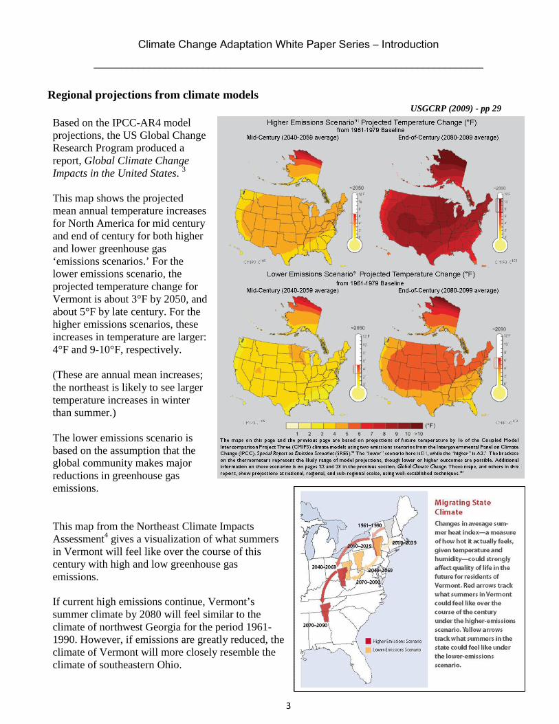
Climate Change Adaptation White Paper Series – Introduction _______________________________________________________________________

3

Regional projections from climate models Based on the IPCC-AR4 model projections, the US Global Change Research Program produced a report, Global Climate Change Impacts in the United States. 3

USGCRP (2009) - pp 29

This map shows the projected mean annual temperature increases for North America for mid century and end of century for both higher and lower greenhouse gas ‘emissions scenarios.’ For the lower emissions scenario, the projected temperature change for Vermont is about 3°F by 2050, and about 5°F by late century. For the higher emissions scenarios, these increases in temperature are larger: 4°F and 9-10°F, respectively.

(These are annual mean increases; the northeast is likely to see larger temperature increases in winter than summer.)

The lower emissions scenario is based on the assumption that the global community makes major reductions in greenhouse gas emissions.

This map from the Northeast Climate Impacts Assessment4 gives a visualization of what summers in Vermont will feel like over the course of this century with high and low greenhouse gas emissions.

If current high emissions continue, Vermont’s summer climate by 2080 will feel similar to the climate of northwest Georgia for the period 1961- 1990. However, if emissions are greatly reduced, the climate of Vermont will more closely resemble the climate of southeastern Ohio.

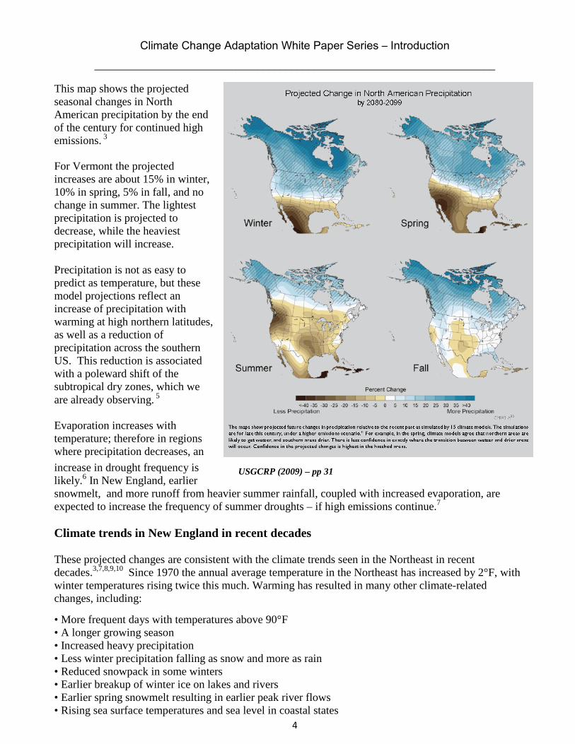
Climate Change Adaptation White Paper Series – Introduction _______________________________________________________________________

4

This map shows the projected seasonal changes in North American precipitation by the end of the century for continued high emissions. 3

For Vermont the projected increases are about 15% in winter, 10% in spring, 5% in fall, and no change in summer. The lightest precipitation is projected to decrease, while the heaviest precipitation will increase.

Precipitation is not as easy to predict as temperature, but these model projections reflect an increase of precipitation with warming at high northern latitudes, as well as a reduction of precipitation across the southern US. This reduction is associated with a poleward shift of the subtropical dry zones, which we are already observing. 5

Evaporation increases with temperature; therefore in regions where precipitation decreases, an increase in drought frequency is likely.6 In New England, earlier

USGCRP (2009) – pp 31

snowmelt, and more runoff from heavier summer rainfall, coupled with increased evaporation, are expected to increase the frequency of summer droughts – if high emissions continue.7

Climate trends in New England in recent decades

These projected changes are consistent with the climate trends seen in the Northeast in recent decades.3,7,8,9,10 Since 1970 the annual average temperature in the Northeast has increased by 2°F, with winter temperatures rising twice this much. Warming has resulted in many other climate-related changes, including:

• More frequent days with temperatures above 90°F • A longer growing season • Increased heavy precipitation • Less winter precipitation falling as snow and more as rain • Reduced snowpack in some winters • Earlier breakup of winter ice on lakes and rivers • Earlier spring snowmelt resulting in earlier peak river flows • Rising sea surface temperatures and sea level in coastal states

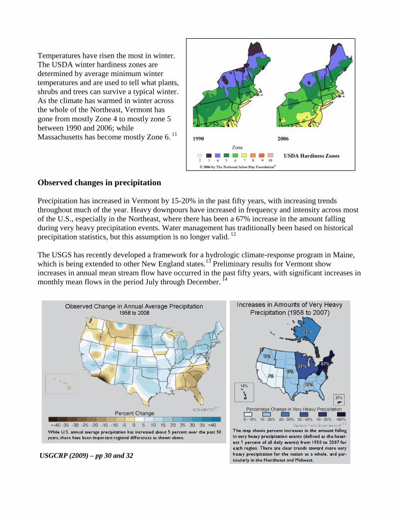
Temperatures have risen the most in winter. The USDA winter hardiness zones are determined by average minimum winter temperatures and are used to tell what plants, shrubs and trees can survive a typical winter. As the climate has warmed in winter across the whole of the Northeast, Vermont has gone from mostly Zone 4 to mostly zone 5 between 1990 and 2006; while Massachusetts has become mostly Zone 6. 11

Observed changes in precipitation

Precipitation has increased in Vermont by 15-20% in the past fifty years, with increasing trends throughout much of the year. Heavy downpours have increased in frequency and intensity across most of the U.S., especially in the Northeast, where there has been a 67% increase in the amount falling during very heavy precipitation events. Water management has traditionally been based on historical precipitation statistics, but this assumption is no longer valid. 12

The USGS has recently developed a framework for a hydrologic climate-response program in Maine, which is being extended to other New England states.13 Preliminary results for Vermont show increases in annual mean stream flow have occurred in the past fifty years, with significant increases in monthly mean flows in the period July through December. 14

USGCRP (2009) – pp 30 and 32

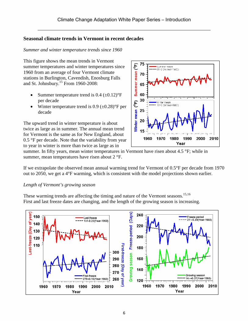
Climate Change Adaptation White Paper Series – Introduction _______________________________________________________________________

6

Seasonal climate trends in Vermont in recent decades Summer and winter temperature trends since 1960

This figure shows the mean trends in Vermont summer temperatures and winter temperatures since 1960 from an average of four Vermont climate stations in Burlington, Cavendish, Enosburg Falls and St. Johnsbury.15 From 1960-2008:

• Summer temperature trend is 0.4 (±0.12)°F

per decade • Winter temperature trend is 0.9 (±0.28)°F per

decade The upward trend in winter temperature is about twice as large as in summer. The annual mean trend for Vermont is the same as for New England, about 0.5 °F per decade. Note that the variability from year to year in winter is more than twice as large as in summer. In fifty years, mean winter temperatures in Vermont have risen about 4.5 °F; while in summer, mean temperatures have risen about 2 °F.

If we extrapolate the observed mean annual warming trend for Vermont of 0.5°F per decade from 1970 out to 2050, we get a 4°F warming, which is consistent with the model projections shown earlier.

Length of Vermont’s growing season

These warming trends are affecting the timing and nature of the Vermont seasons.15,16

First and last freeze dates are changing, and the length of the growing season is increasing.

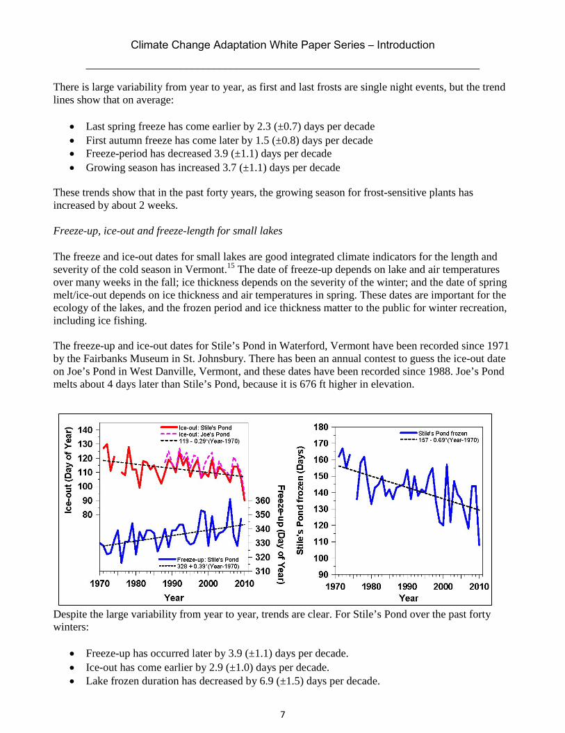
Climate Change Adaptation White Paper Series – Introduction _______________________________________________________________________

7

There is large variability from year to year, as first and last frosts are single night events, but the trend lines show that on average:

• Last spring freeze has come earlier by 2.3 (±0.7) days per decade • First autumn freeze has come later by 1.5 (±0.8) days per decade • Freeze-period has decreased 3.9 (±1.1) days per decade • Growing season has increased 3.7 (±1.1) days per decade

These trends show that in the past forty years, the growing season for frost-sensitive plants has increased by about 2 weeks.

Freeze-up, ice-out and freeze-length for small lakes

The freeze and ice-out dates for small lakes are good integrated climate indicators for the length and severity of the cold season in Vermont.15 The date of freeze-up depends on lake and air temperatures over many weeks in the fall; ice thickness depends on the severity of the winter; and the date of spring melt/ice-out depends on ice thickness and air temperatures in spring. These dates are important for the ecology of the lakes, and the frozen period and ice thickness matter to the public for winter recreation, including ice fishing.

The freeze-up and ice-out dates for Stile’s Pond in Waterford, Vermont have been recorded since 1971 by the Fairbanks Museum in St. Johnsbury. There has been an annual contest to guess the ice-out date on Joe’s Pond in West Danville, Vermont, and these dates have been recorded since 1988. Joe’s Pond melts about 4 days later than Stile’s Pond, because it is 676 ft higher in elevation.

Despite the large variability from year to year, trends are clear. For Stile’s Pond over the past forty winters:

• Freeze-up has occurred later by 3.9 (±1.1) days per decade. • Ice-out has come earlier by 2.9 (±1.0) days per decade. • Lake frozen duration has decreased by 6.9 (±1.5) days per decade.

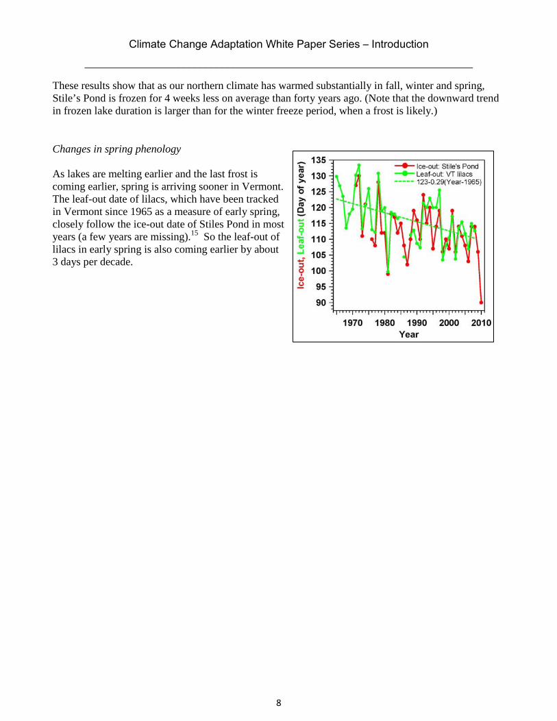
Climate Change Adaptation White Paper Series – Introduction _______________________________________________________________________

8

These results show that as our northern climate has warmed substantially in fall, winter and spring, Stile’s Pond is frozen for 4 weeks less on average than forty years ago. (Note that the downward trend in frozen lake duration is larger than for the winter freeze period, when a frost is likely.)

Changes in spring phenology

As lakes are melting earlier and the last frost is coming earlier, spring is arriving sooner in Vermont. The leaf-out date of lilacs, which have been tracked in Vermont since 1965 as a measure of early spring, closely follow the ice-out date of Stiles Pond in most years (a few years are missing).15 So the leaf-out of lilacs in early spring is also coming earlier by about 3 days per decade.

Climate Change Adaptation White Paper Series – Introduction _______________________________________________________________________

9

Summary of expected changes in the climate of Vermont The observed changes in Vermont’s climate over the past fifty years match those seen in New England. These changes are also consistent with the changes projected by global climate models through 2050. Winter temperatures are rising fastest, so the winter season is shrinking and becoming less severe. Spring is coming earlier and fall later, so the summer growing season is lengthening. As the climate warms, total precipitation in Vermont is expected to increase in all seasons except summer. The frequency of heavy precipitation events is likely to increase in all seasons, with the heaviest precipitation events occurring in the summer season. Stream flow is likely to increase.

Although we cannot predict in detail the changes in weather patterns resulting from climate change, we can summarize the seasonal changes we are likely to see in Vermont in the coming decades:

In winter:

• Later arrival of winter • Warmer winters: upward shift of USDA climate zones • More overwintering of pests • Shortened ski, snowmobile, ice-fishing, and snowshoeing season • Increased winter precipitation • More wet snow and freezing rain • Multiple melt events in the winter with possible flooding

In spring: • Reduced productivity of sugar maples • Earlier end to sugaring season • Earlier spring melt and run-off; possibly larger stream flows • Earlier arrival of spring • Earlier bloom dates of many plant species • Earlier last spring frost • Earlier ice-out of lakes and ponds

In summer: • Hotter summers • Reduced productivity of cold-weather crops • Reduced productivity of dairy cows • Longer growing season • More heavy rain events • More frequent floods and associated flood damage • Greater frequency of 1-2 month droughts • Increased warm-weather pest species, such as mosquitoes, ticks, and algae • Increased threats to cold-water fish and wildlife species • Increased hazards to human health, including heat waves and the spread of disease • Increased hazards to human safety, such as landslides, flooding, and violent storm events • Increased threat to infrastructure, such as roads and bridges near streams and rivers • Worsening air quality in some areas

In fall: • Later first fall frost • Warmer fall temperatures • Later fall color • Increased fall precipitation and stream flow

10

10

References

1. Lacis, A.A., G.A. Schmidt, D. Rind and R.A. Ruedy (2010): Atmospheric CO2: Principal Control Knob Governing Earth’s Temperature. Science, 330, 356-359. DOI:10.1126/science.1190653.

2. IPCC (2007): Climate Change 2007: Synthesis Report. Pachauri, R. K., and A. Reisinger, Eds. http://www.ipcc.ch/pdf/assessment-report/ar4/syr/ar4_syr.pdf

3. USGCRP (2009): Global Climate Change Impacts in the United States. U.S. Global Change Research Program. http://downloads.globalchange.gov/usimpacts/pdfs/climate-impacts-report.pdf

4. NECIA (2007): Vermont. Confronting Climate Change in the U.S.Northeast. http://www.climatechoices.org/assets/documents/climatechoices/vermont_necia.pdf

5. Zhou, Y. P. K-M. Xu, Y. C. Sud and A.K. Betts (2011), Recent Trends of Tropical Hydrological Cycle Inferred from GPCP and ISCCP Data. J. Geophys. Res., 116, D09101, doi:10.1029/2010JD015197.

6. Dai, A. (2011): Drought under global warming: a review. WIRES Clim. Change, 2, 45-65. DOI: 10.1002/wcc.81.

7. Frumhoff, P. C., J. J. McCarthy, J. M. Melillo, S. C. Moser, and D. J. Wuebbles, 2007: Confronting climate change in the U.S. Northeast: Science, impacts and solutions. Northeast Climate Impacts Assessment (NECIA), Union of Concerned Scientists, Synthesis Rep., 160 pp. http://www.climatechoices.org/assets/documents/climatechoices/confronting-climate-change-in-the-u-s-northeast.pdf

8. Hayhoe, K., Wake, C.P., Huntington, T.G., Luo, L., Schwartz, M.D., Sheffield, J., Wood, E., Anderson, B., Bradbury, J., DeGaetano, A., Troy, T.J., and D. Wolfe (2007): Past and future changes in climate and hydrological indicators in the US Northeast. Climate Dynamics, 28, 381-407.

9. NECIA (2006): Climate Change in the U.S. Northeast. http://www.climatechoices.org/assets/documents/climatechoices/NECIA_climate_report_final.pdf

10. Burakowski, E.A., C.P. Wake, B. Braswell, and D.P. Brown (2008): Trends in wintertime climate in the northeastern United States: 1965–2005. J. Geophys. Res., 113, D20114, doi:10.1029/2008JD009870.

11. Arbor Day Foundation maps. http://www.arborday.org/media/map_change.cfm

12. Milly, P.C.D., J. Betancourt, M. Falkenmark, R.M. Hirsch, Z.W. Kundzewicz, D.P. Lettenmaier, and R.J. Stouffer (2008): Stationarity is dead: Whither water management? Science, 319, 573-574.

13. Hodgkins G.A., R.M. Lent, R.W. Dudley and C.W. Schalk (2009): Framework for a U.S. Geological Survey Hydrologic Climate-Response Program in Maine. U.S. Geological Survey Open-File Report 2009–1115, 34pp. http://pubs.usgs.gov/of/2009/1115/

14. Hodgkins et al. (2010): Trends in Streamflow Characteristics at Selected Streamgages in Vermont. Draft manuscript.

15. Betts, A. K. (2011a), Vermont Climate Change Indicators. Weather, Climate and Society, 3, doi: 10.1175/2011WCAS1096.1. (In press, available at http://alanbetts.com/research)

16. Betts, A. K. (2011b), Seasonal Climate Transitions in New England. Weather, 66, doi: 10.1002/wea.754. (In press, available at http://alanbetts.com/research)

Preparation of this report was supported in part by NSF grant AGS05-29797. Document available at http://www.anr.state.vt.us/anr/climatechange/Adaptation.html