
Manual - CivilTech · AllPile can handle all types of piles: drilled shaft, driven pile, auger-cast...
103
User’s Manual Volume 1 and 2 CivilTech Software 2017 AllPile Version 7
Transcript of Manual - CivilTech · AllPile can handle all types of piles: drilled shaft, driven pile, auger-cast...

CivilTech Software
User’s Manual
Volume 1 and 2
CivilTech Software 2017
AllPile Version 7
CivilTech Software
All the information, including technical and engineering data, processes, and
results, presented in this program have been prepared according to recognized
contracting and/or engineering principles, and are for general information
only. If anyone uses this program for any specific application without an
independent competent professional examination and verification of its
accuracy, suitability, and applicability by a licensed professional engineer,
he/she does so at his/her own risk and assumes any and all liability resulting
from such use. In no event shall CivilTech be held liable for any damages
including lost profits, lost savings, or other incidental or consequential
damages resulting from the use of or inability to use the information
contained within.
Information in this document is subject to change without notice and does not
represent a commitment on the part of CivilTech. This program is furnished
under a license agreement, and the program may be used only in accordance
with the terms of the agreement. The program may be copied for backup
purposes only.
The program or user’s guide shall not be reproduced, stored in a retrieval
system, or transmitted in any form or by any means, electronic, mechanical,
photocopying, recording, or otherwise, without prior written consent from
CivilTech.
Copyright 2017 CivilTech Software. All rights reserved.
Simultaneously published in the U.S. and Canada.
Printed and bound in the United States of America.
Published by
CivilTech Software
Web Site: http://www.civiltech.com
2
TABLE OF CONTENTS
VOLUME 1
CHAPTER 1 INTRODUCTION .................................................................. 4 1.1 ABOUT ALLPILE .......................................................................................................................................... 4 1.2 ABOUT THE MANUAL................................................................................................................................... 4 1.3 ABOUT THE COMPANY ................................................................................................................................. 4
CHAPTER 2 INSTALLATION AND ACTIVATION ................................................................... 5 2.1 INSTALLATION AND RUN .............................................................................................................................. 5
CHAPTER 3 OVERVIEW .............................................................................................................. 8 3.1 PROGRAM OUTLINE ..................................................................................................................................... 8 3.2 PROGRAM INTERFACE.................................................................................................................................. 9 3.3 PULL-DOWN MENUS .................................................................................................................................. 10
3.3.1 FILE .................................................................................................................................................... 10 3.3.2 EDIT ................................................................................................................................................... 10 3.3.3 RUN .................................................................................................................................................... 11 3.3.4 SETUP ................................................................................................................................................. 11 3.3.5 HELP ................................................................................................................................................... 11
3.4 SPEED BAR ................................................................................................................................................ 12 3.5 SAMPLE AND TEMPLATES .......................................................................................................................... 12
CHAPTER 4 DATA INPUT............................................................................................................ 13 4.1 INPUT PAGES ............................................................................................................................................. 13 4.2 PILE TYPE PAGE ........................................................................................................................................ 13
4.2.1 PROJECT TITLES ................................................................................................................................. 14 4.2.2 COMMENTS ........................................................................................................................................ 14 4.2.3 UNITS ................................................................................................................................................. 14
4.3 PILE PROFILE PAGE .................................................................................................................................... 15 4.4 PILE PROPERTIES PAGE ............................................................................................................................... 17
4.4.1 PILE PROPERTY TABLE ....................................................................................................................... 17 4.4.2 ADD TIP SECTION ............................................................................................................................... 18 4.4.2 ADD TIP SECTION ............................................................................................................................... 19 4.4.3 PILE SECTION SCREEN ........................................................................................................................ 19 4.4.4 EFFECTIVE AREA AND TOTAL AREA ................................................................................................... 22 4.4.5 SHALLOW FOOTING ............................................................................................................................ 23
4.5 LOAD AND GROUP ..................................................................................................................................... 25 4.5.1 SINGLE PILE ........................................................................................................................................ 25 4.5.2 GROUP PILES ...................................................................................................................................... 27 4.5.3 TOWER FOUNDATION ......................................................................................................................... 29
4.6 SOIL PROPERTY PAGE ................................................................................................................................. 30 4.6.1 SOIL PROPERTY TABLE ............................................................................................................................. 31 4.6.2 SOIL PARAMETER SCREEN .................................................................................................................. 33
4.7 ADVANCED PAGE ...................................................................................................................................... 35 4.7.1 ZERO RESISTANCE AND NEGATIVE RESISTANCE (DOWNDRAG FORCE) .............................................. 35
4.8 UNITS OF MEASURE ................................................................................................................................... 38
CHAPTER 5 RESULTS .................................................................................................................. 39 5.1 PROFILE ..................................................................................................................................................... 39 5.2 VERTICAL ANALYSIS RESULTS .................................................................................................................. 39
5.2.1 DEPTH (Z) VS. S, F, Q .......................................................................................................................... 40
3
. . . . . . . . .
5.2.2 LOAD VS. SETTLEMENT ...................................................................................................................... 41 5.2.3 CAPACITY VS. LENGTH ....................................................................................................................... 41 5.2.4 T-Z CURVE .......................................................................................................................................... 42 5.2.5 Q-W CURVE ........................................................................................................................................ 42 5.2.6 SUBMITTAL REPORT ........................................................................................................................... 43 5.2.7 SUMMARY REPORT ............................................................................................................................. 43 5.2.8 DETAIL REPORT .................................................................................................................................. 43 5.2.9 EXPORTING TO EXCEL ........................................................................................................................ 44 5.2.10 FIGURE NUMBER ................................................................................................................................ 44
5.3 LATERAL ANALYSIS RESULTS .................................................................................................................... 44 5.3.1 DEPTH (Z) VS. YT, M, P AND PRESSURES ............................................................................................. 44 5.3.2 LOAD (P) - YT, M ................................................................................................................................ 45 5.3.3 DEPTH VS. YT ...................................................................................................................................... 46 5.3.4 DEPTH VS. M ...................................................................................................................................... 46 5.3.5 P-Y CURVE .......................................................................................................................................... 47 5.3.6 SUBMITTAL REPORT ........................................................................................................................... 47 5.3.7 SUMMARY REPORT ............................................................................................................................. 47 5.3.8 COM624S OUTPUT/INPUT ................................................................................................................... 47 5.3.9 EXPORTING TO EXCEL ........................................................................................................................ 48 5.3.10 FIGURE NUMBER ................................................................................................................................ 48
5.4 STIFFNESS [ K] RESULTS ............................................................................................................................ 48 5.5 PREVIEW AND PRINT SCREEN .................................................................................................................... 49 5.6 ERRORS AND TROUBLESHOOTING .............................................................................................................. 50
CHAPTER 6 SETUP ....................................................................................................................... 52 6.1 SETUP SCREEN ........................................................................................................................................... 52 6.2 PULL-DOWN MENU: SETUP ....................................................................................................................... 52 6.3 SPEED BAR ................................................................................................................................................ 53 6.4 TABBED PAGES .......................................................................................................................................... 53
6.4.1 REPORT FORMAT PAGE ...................................................................................................................... 53 6.4.2 MATERIALS PAGE ............................................................................................................................... 54 6.4.3 PILE TYPE PAGE ................................................................................................................................. 56
CHAPTER 7 SAMPLES ................................................................................................................. 58 7.1 SAMPLES.................................................................................................................................................... 58
VOLUME 2
SEE PAGE 59 FOR Table of Contents
4
. . . . . . . . .
CHAPTER 1 INTRODUCTION
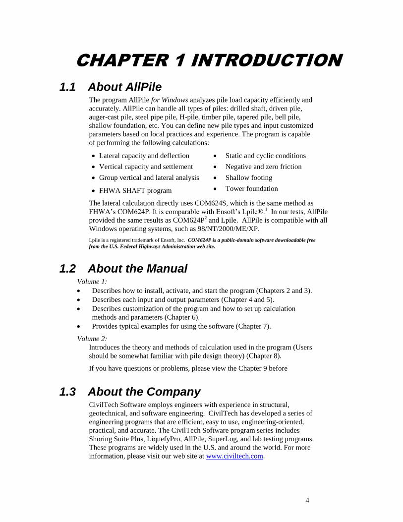
1.1 About AllPile The program AllPile for Windows analyzes pile load capacity efficiently and
accurately. AllPile can handle all types of piles: drilled shaft, driven pile,
auger-cast pile, steel pipe pile, H-pile, timber pile, tapered pile, bell pile,
shallow foundation, etc. You can define new pile types and input customized
parameters based on local practices and experience. The program is capable
of performing the following calculations:
Lateral capacity and deflection
Vertical capacity and settlement
Group vertical and lateral analysis
FHWA SHAFT program
Static and cyclic conditions
Negative and zero friction
Shallow footing
Tower foundation
The lateral calculation directly uses COM624S, which is the same method as
FHWA’s COM624P. It is comparable with Ensoft’s Lpile®.1 In our tests, AllPile
provided the same results as COM624P2 and Lpile. AllPile is compatible with all
Windows operating systems, such as 98/NT/2000/ME/XP.
Lpile is a registered trademark of Ensoft, Inc. COM624P is a public-domain software downloadable free
from the U.S. Federal Highways Administration web site.
1.2 About the Manual Volume 1:
Describes how to install, activate, and start the program (Chapters 2 and 3).
Describes each input and output parameters (Chapter 4 and 5).
Describes customization of the program and how to set up calculation
methods and parameters (Chapter 6).
Provides typical examples for using the software (Chapter 7).
Volume 2:
Introduces the theory and methods of calculation used in the program (Users
should be somewhat familiar with pile design theory) (Chapter 8).
If you have questions or problems, please view the Chapter 9 before
1.3 About the Company CivilTech Software employs engineers with experience in structural,
geotechnical, and software engineering. CivilTech has developed a series of
engineering programs that are efficient, easy to use, engineering-oriented,
practical, and accurate. The CivilTech Software program series includes
Shoring Suite Plus, LiquefyPro, AllPile, SuperLog, and lab testing programs.
These programs are widely used in the U.S. and around the world. For more
information, please visit our web site at www.civiltech.com.
5
. . . . . . . . .
CHAPTER 2 INSTALLATION
AND ACTIVATION
2.1 Installation and Run USB key:
If you have CivilTech
USB key, the
program is inside the
key.
Introduction of USB key
Civiltech USB key functions the same way as a USB flash drive,
(or called memory sticks or jump drive), but with a special chipset
inside. It has a memory of 128 MB, and USB 2.0 connectivity. The
key is compatible with Windows 2000, Xp, 7, 8 and higher, but
may not work with Windows 98 (You need to install USB driver
for Win98).
Insert the key into any USB port in your computer. If you do not
have an extra USB port, you should buy a USB extension cord
(about $10-$20)
Wait until the small light on the back of the USB key stops
flashing and stays red. This means that Windows has detected the
USB key. A small panel may pop up that says “USB mass storage
device found”, you can either close this panel or click “OK”.
Do not remove the key while the light is blinking, as that will
damage the key. You can remove the key only during the following
situations:
1. Your computer is completely turned off, or
2. You have safely ejected the key from the system. You can do
this by going down to the Windows task bar, finding the icon
that says “Unplug or Eject Hardware” (usually located at the
bottom right-hand side of the screen) and clicking on that. It
will then tell you when it is safe to remove the hardware.
Running the Program within the Key.
No installation is required.
After you insert the key, use Windows Explorer (or click My
Computer) to check the USB drive (on most computers, it is either
called D:, E:, or F:). You will find some files inside. There is a
folder called “/Keep” inside. Do not change, remove, or delete this
folder or the files inside, or else your key will become void.
You will find a folder called “/AllPile7”. Open this folder and find
AllPile.exe. Double click this program to run AllPile from your key.
You can also create a new folder, save and open your project files
directly to and from your key. There should be enough room on the
6
. . . . . . . . .
key for your files.
The manual is also located in the key in the root directory. Double-
click on the file to open it. You need Adobe PDF to read this file,
which is downloadable free of charge from Adobe’s website.
(http://www.adobe.com)
The USB key cannot be plugged in a network server and used by
many stations. It may damage the USB key.
Running the Program from your Hard Disk:
You can also run the program from your hard disk; the program
may run a little bit faster from your hard disk.
There is a file called al_setup.exe in the root directory of the key.
Double-click on the file to start installation.
The installation process will help you to install the program on
your local hard disk. Installation to network drive or disk is not
recommended. The program may not work properly.
The installation will create a shortcut on your desktop. Click the
icon to start the program.
You still need to plug the USB key into the USB port to run the
program. It will automatically detect the USB key.
The key activation status can be checked from Help manual under
Activation.
No USB key:
If you received the
program from email
or from download…
Installation:
The installation file is called al_setup.exe. Click it will start up the
installation process automatically. The installation process will help you to
install the program on your local hard disk and create a shortcut on your
desktop.
Activation:
Follow the instruction from Email we sent to you to open Activation
panel.
The CPU number is shown on the panel. This is a unique number for
your computer, which must be reported to CivilTech by email. The
email can be found on our web side: http://www.civiltech.com.
An Activation Code will email back to you after we verify you have
purchased the program.
Input the Activation Code in the Activation Pane, and then close the
program.
Click the icon to start the program, which has full function now.
7
. . . . . . . . .
Download Manual
from Internet
The most updated manual for AllPile can be downloaded from our
Web site (www.civiltech.com/software/download.html). Click on
AllPile Manual link to open the manual, (you must have Adobe
Acrobat Reader to open the file). Then, save the PDF file onto your
hard drive.
Quitting the
Program
From the File menu, select [Exit] or Ctrl+X.
Input Firm and User
Name
From the Help menu, select Firm and User. Once the panel pulls
out, enter in your firm’s name and the user’s name. This information
will be printed in the report.
About Program From the Help menu, select About. This will provide you with the
version of the program. Click anywhere on the screen to exit back to
the program.
Note: The program is not compatible for networking. You cannot
install the program on your network server and run it from
workstations. The program is one copy per license, which can only be
installed in one workstation.
Problem, Questions & Answers and Troubleshooting
If you encounter any problems, please save your data file and send us an email with the input files
for each module. Most time, telephone call cannot solve the problem. Attached input files and
email can solve the problem quickly. Email: [email protected]. Please review Chapter
9, Questions & Answers before contact us.
If you need administrative assistance such as USB problem, please email your request to
8
. . . . . . . . .
CHAPTER 3 OVERVIEW
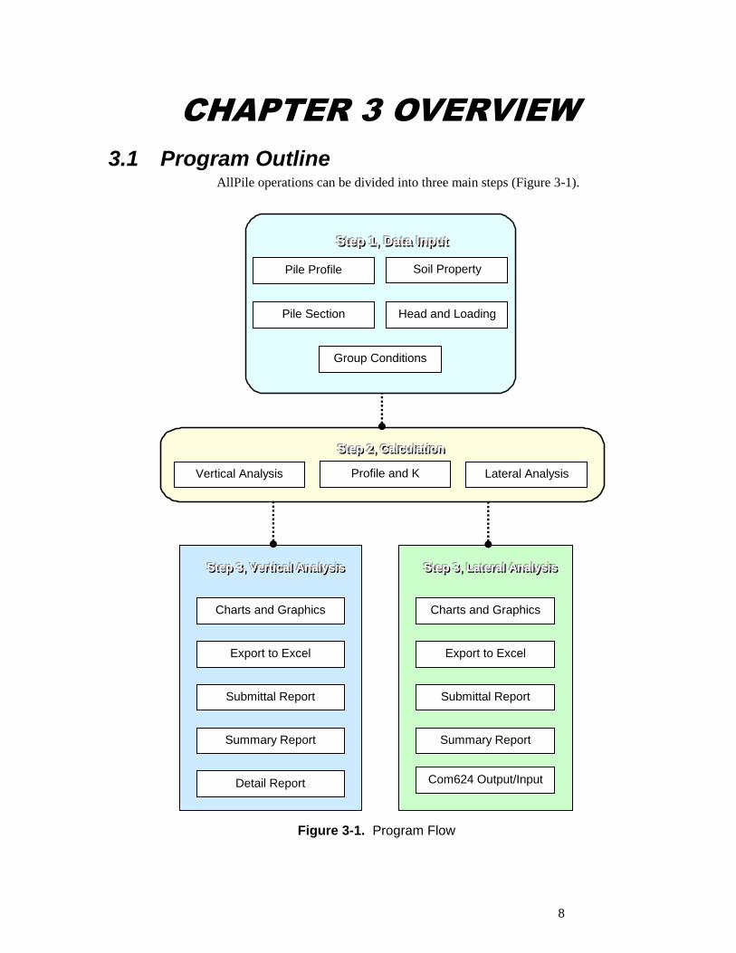
3.1 Program Outline AllPile operations can be divided into three main steps (Figure 3-1).
SSSttteeeppp 333,,, VVVeeerrrttt iiicccaaalll AAAnnnaaalllyyysssiiisss SSSttteeeppp 333,,, LLLaaattteeerrraaalll AAAnnnaaalllyyysssiiisss
Charts and Graphics Charts and Graphics
Export to Excel Export to Excel
Submittal Report Submittal Report
Summary Report
Detail Report
Summary Report
Com624 Output/Input
Figure 3-1. Program Flow
SSSttteeeppp 222,,, CCCaaalllcccuuulllaaattt iiiooonnn
Vertical Analysis Lateral Analysis Profile and K
SSSttteeeppp 111,,, DDDaaatttaaa IIInnnpppuuuttt
Pile Profile
Pile Section
Group Conditions
Head and Loading
Soil Property
9
. . . . . . . . .
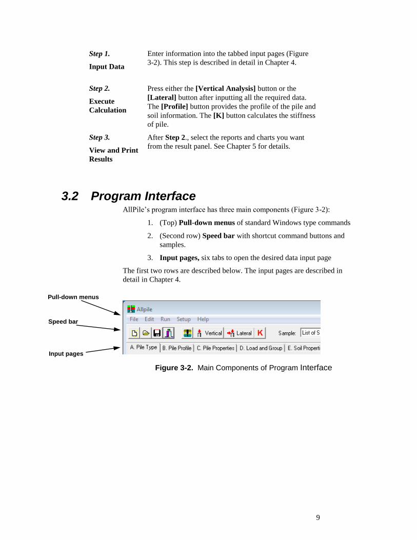
Step 1.
Input Data
Enter information into the tabbed input pages (Figure
3-2). This step is described in detail in Chapter 4.
Step 2.
Execute
Calculation
Press either the [Vertical Analysis] button or the
[Lateral] button after inputting all the required data.
The [Profile] button provides the profile of the pile and
soil information. The [K] button calculates the stiffness
of pile.
Step 3.
View and Print
Results
After Step 2., select the reports and charts you want
from the result panel. See Chapter 5 for details.
3.2 Program Interface AllPile’s program interface has three main components (Figure 3-2):
1. (Top) Pull-down menus of standard Windows type commands
2. (Second row) Speed bar with shortcut command buttons and
samples.
3. Input pages, six tabs to open the desired data input page
The first two rows are described below. The input pages are described in
detail in Chapter 4.
Figure 3-2. Main Components of Program Interface
Pull-down menus
Speed bar
Input pages
10
. . . . . . . . .
3.3 Pull-Down Menus
HINT: You can use the F key such as F4, F5, F10 to execute functions.
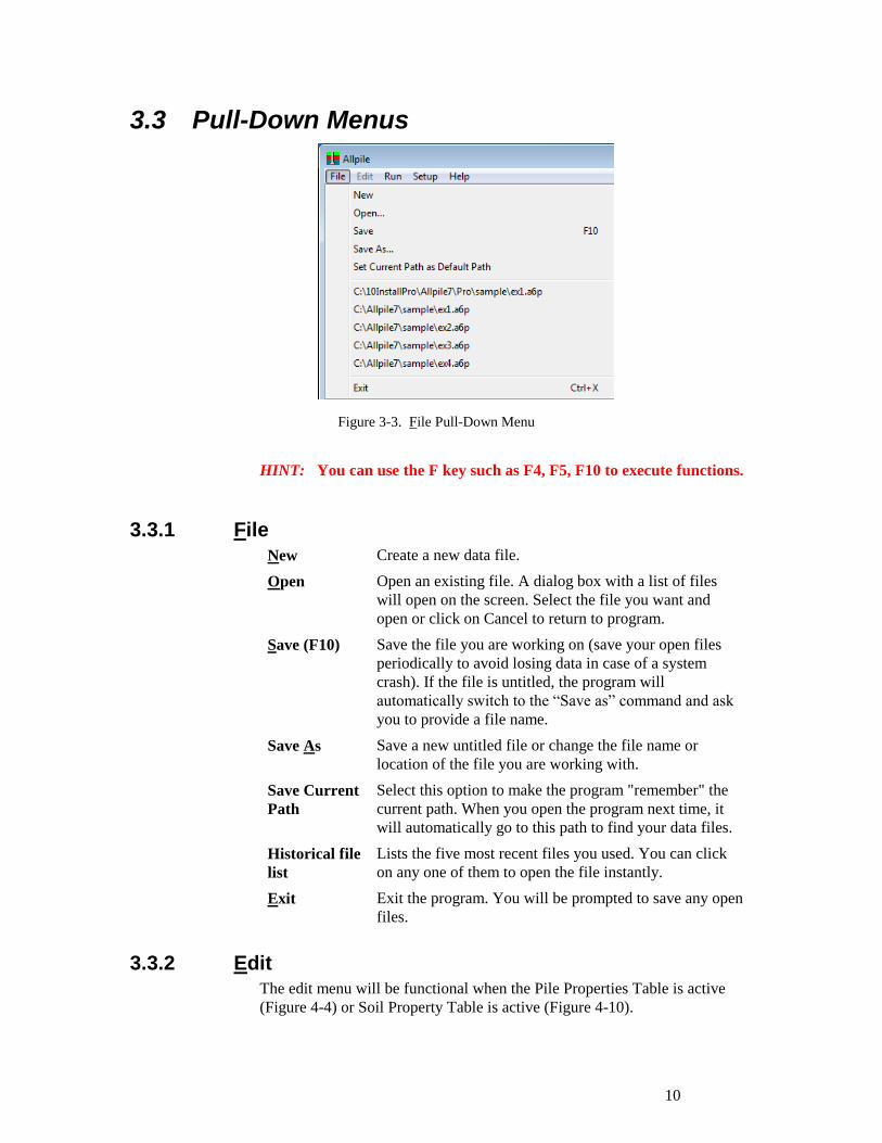
3.3.1 File
New Create a new data file.
Open Open an existing file. A dialog box with a list of files
will open on the screen. Select the file you want and
open or click on Cancel to return to program.
Save (F10)
Save the file you are working on (save your open files
periodically to avoid losing data in case of a system
crash). If the file is untitled, the program will
automatically switch to the “Save as” command and ask
you to provide a file name.
Save As Save a new untitled file or change the file name or
location of the file you are working with.
Save Current
Path
Select this option to make the program "remember" the
current path. When you open the program next time, it
will automatically go to this path to find your data files.
Historical file
list
Lists the five most recent files you used. You can click
on any one of them to open the file instantly.
Exit Exit the program. You will be prompted to save any open
files.
3.3.2 Edit The edit menu will be functional when the Pile Properties Table is active
(Figure 4-4) or Soil Property Table is active (Figure 4-10).
Figure 3-3. File Pull-Down Menu
11
. . . . . . . . .
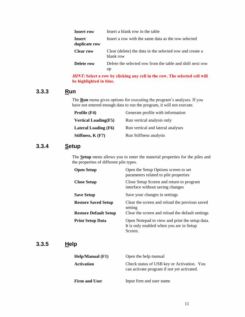
Insert row Insert a blank row in the table
Insert
duplicate row
Insert a row with the same data as the row selected
Clear row Clear (delete) the data in the selected row and create a
blank row
Delete row Delete the selected row from the table and shift next row
up
HINT: Select a row by clicking any cell in the row. The selected cell will
be highlighted in blue.
3.3.3 Run
The Run menu gives options for executing the program’s analyses. If you
have not entered enough data to run the program, it will not execute.
Profile (F4) Generate profile with information
Vertical Loading(F5) Run vertical analysis only
Lateral Loading (F6) Run vertical and lateral analyses
Stiffness, K (F7) Run Stiffness analysis
3.3.4 Setup
The Setup menu allows you to enter the material properties for the piles and
the properties of different pile types.
Open Setup Open the Setup Options screen to set
parameters related to pile properties
Close Setup Close Setup Screen and return to program
interface without saving changes
Save Setup Save your changes in settings
Restore Saved Setup Clear the screen and reload the previous saved
setting
Restore Default Setup Clear the screen and reload the default settings
Print Setup Data Open Notepad to view and print the setup data.
It is only enabled when you are in Setup
Screen.
3.3.5 Help
Help/Manual (F1) Open the help manual
Activation Check status of USB key or Activation. You
can activate program if not yet activated.
Firm and User Input firm and user name
12
. . . . . . . . .
About Display information about the version of your
program.
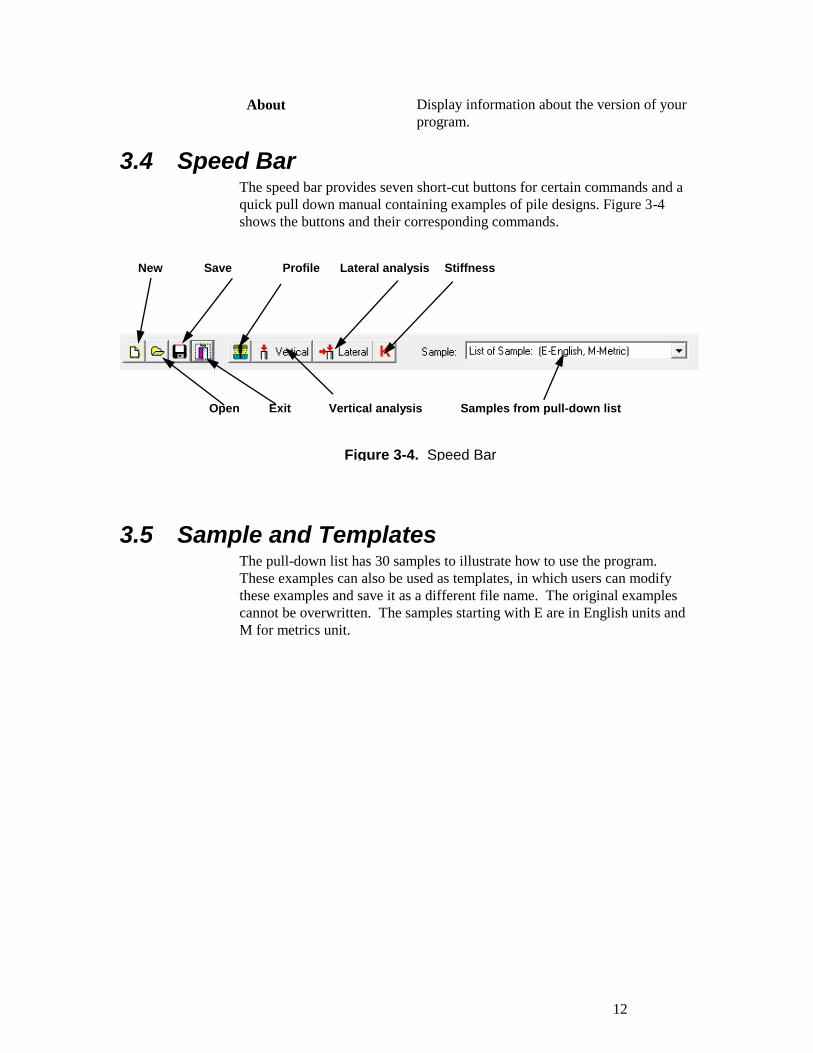
3.4 Speed Bar The speed bar provides seven short-cut buttons for certain commands and a
quick pull down manual containing examples of pile designs. Figure 3-4
shows the buttons and their corresponding commands.
3.5 Sample and Templates The pull-down list has 30 samples to illustrate how to use the program.
These examples can also be used as templates, in which users can modify
these examples and save it as a different file name. The original examples
cannot be overwritten. The samples starting with E are in English units and
M for metrics unit.
New Save Profile Lateral analysis Stiffness
Figure 3-4. Speed Bar
Open Exit Vertical analysis Samples from pull-down list
13
. . . . . . . . .
CHAPTER 4 DATA INPUT
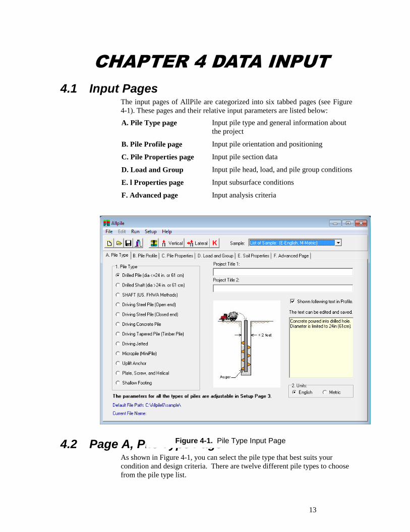
4.1 Input Pages The input pages of AllPile are categorized into six tabbed pages (see Figure
4-1). These pages and their relative input parameters are listed below:
A. Pile Type page Input pile type and general information about
the project
B. Pile Profile page Input pile orientation and positioning
C. Pile Properties page Input pile section data
D. Load and Group Input pile head, load, and pile group conditions
E. l Properties page Input subsurface conditions
F. Advanced page Input analysis criteria
4.2 Page A, Pile Type Page As shown in Figure 4-1, you can select the pile type that best suits your
condition and design criteria. There are twelve different pile types to choose
from the pile type list.
Figure 4-1. Pile Type Input Page
14
. . . . . . . . .
1. Drilled pile diameter less than or equal to 24 inches, such as auger cast
2. Drilled pile diameter is more than 24 inches, such as drilled shaft or pier
3. Shaft using US FHWA SHAFT methods of analysis
4. Driving steel pile with opened end, such as H-pile or open-end pipe. For
plugged condition or friction inside of pile, refer to 4.4.4 of this chapter
and Chapter 8, Section 8.7. You can add a tip section to specify partially
open/close.
5. Driving steel pipe with closed end including pipe with shoe on the tip
6. Driving concrete pile: such as pre-cased circular or square concrete pile
7. Driving timber pile: tapered pile with small tip and large top
8. Driving jetted pile: soils are jetted during driving
9. Micropile: is a pressure-grouted small-diameter pile, also called mini-pile.
10. Uplift anchor: frictionless steel bar with grouted ends (uplift only)
11. Plate, Screw, and Helical: frictionless steel bar with concrete or steel
plates at the end (uplift only)
12. Shallow footing, spread footing for shallow foundations
NOTE: The parameters of each pile type can be customized in the Setup
Screen (Chapter 6).
4.2.1 Project Titles The project title and subtitle can be input in these two boxes. The text will
appear in the report. The location and font can be customized in the Setup
screen described in Chapter 6.
4.2.2 Comments
The Comments box is for additional comments or descriptions of the project.
You can choose to include this message in the profile section of the report by
checking the Show text in Profile page.
4.2.3 Units Select between English or Metric units to be used throughout the program. If
you change the units after input of data, the data you have entered will
automatically convert to the units specified. However, the data will not be
exactly the same after some truncation during conversion.
15
. . . . . . . . .
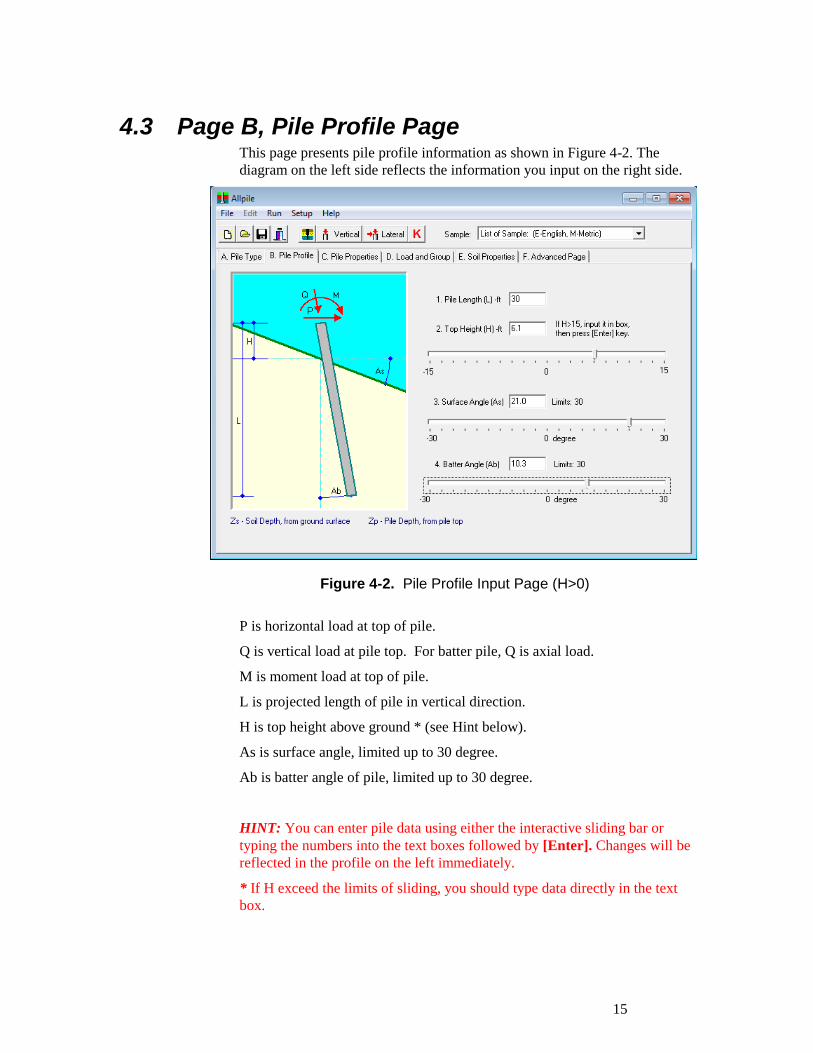
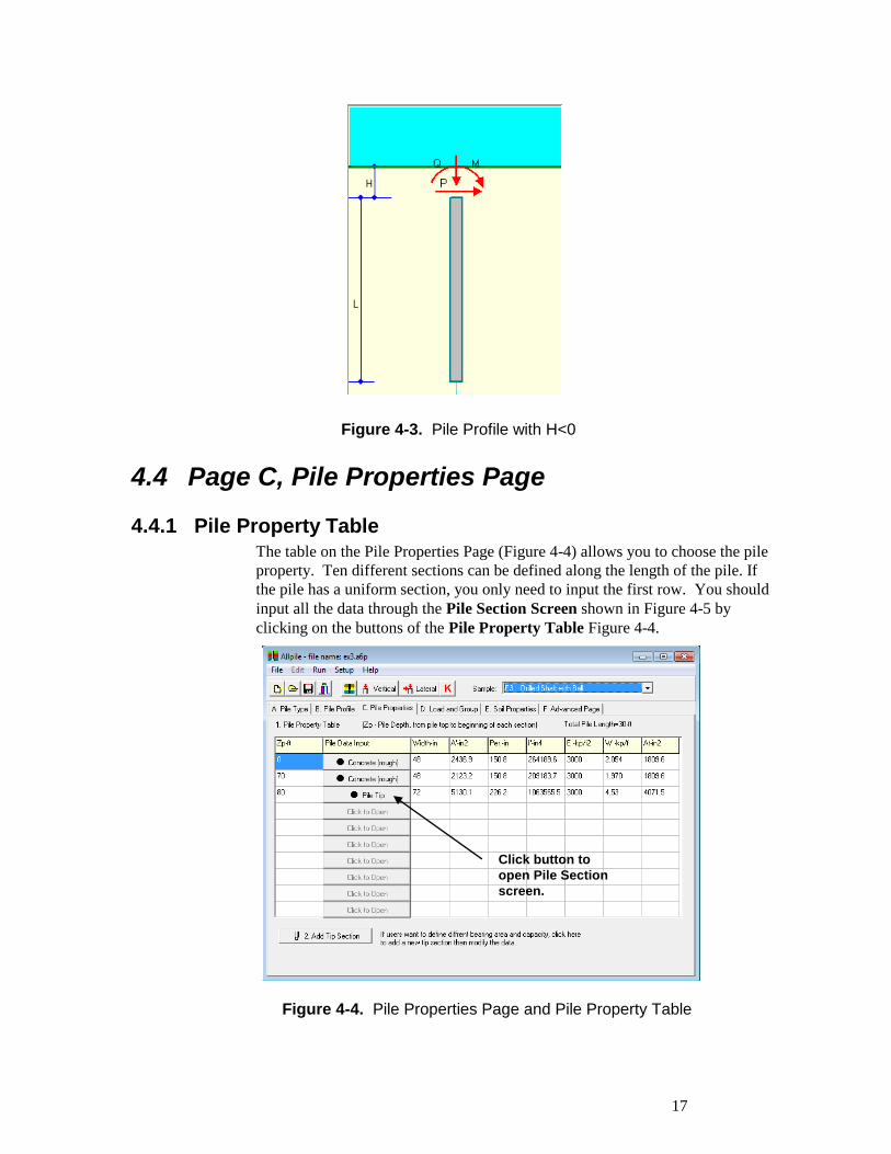
4.3 Page B, Pile Profile Page This page presents pile profile information as shown in Figure 4-2. The
diagram on the left side reflects the information you input on the right side.
P is horizontal load at top of pile.
Q is vertical load at pile top. For batter pile, Q is axial load.
M is moment load at top of pile.
L is projected length of pile in vertical direction.
H is top height above ground * (see Hint below).
As is surface angle, limited up to 30 degree.
Ab is batter angle of pile, limited up to 30 degree.
HINT: You can enter pile data using either the interactive sliding bar or
typing the numbers into the text boxes followed by [Enter]. Changes will be
reflected in the profile on the left immediately.
* If H exceed the limits of sliding, you should type data directly in the text
box.
Figure 4-2. Pile Profile Input Page (H>0)
16
. . . . . . . . .
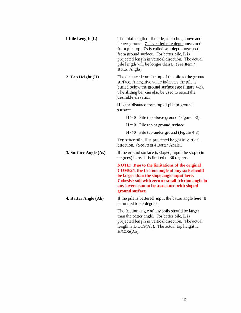
1 Pile Length (L) The total length of the pile, including above and
below ground. Zp is called pile depth measured
from pile top. Zs is called soil depth measured
from ground surface. For better pile, L is
projected length in vertical direction. The actual
pile length will be longer than L (See Item 4
Batter Angle).
2. Top Height (H) The distance from the top of the pile to the ground
surface. A negative value indicates the pile is
buried below the ground surface (see Figure 4-3).
The sliding bar can also be used to select the
desirable elevation.
H is the distance from top of pile to ground
surface:
H > 0 Pile top above ground (Figure 4-2)
H = 0 Pile top at ground surface
H < 0 Pile top under ground (Figure 4-3)
For better pile, H is projected height in vertical
direction. (See Item 4 Batter Angle).
3. Surface Angle (As) If the ground surface is sloped, input the slope (in
degrees) here. It is limited to 30 degree.
NOTE: Due to the limitations of the original
COM624, the friction angle of any soils should
be larger than the slope angle input here.
Cohesive soil with zero or small friction angle in
any layers cannot be associated with sloped
ground surface.
4. Batter Angle (Ab) If the pile is battered, input the batter angle here. It
is limited to 30 degree.
The friction angle of any soils should be larger
than the batter angle. For batter pile, L is
projected length in vertical direction. The actual
length is L/COS(Ab). The actual top height is
H/COS(Ab).
17
. . . . . . . . .
4.4 Page C, Pile Properties Page
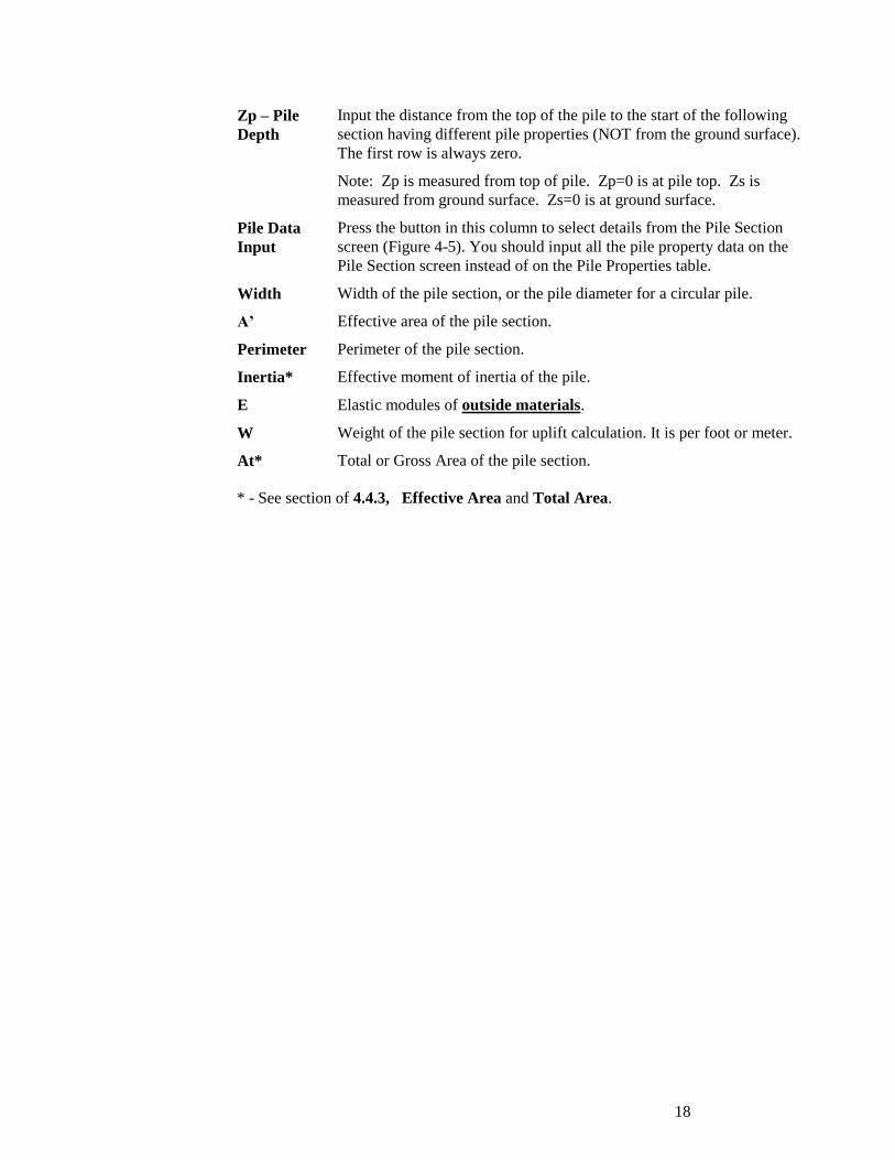
4.4.1 Pile Property Table The table on the Pile Properties Page (Figure 4-4) allows you to choose the pile
property. Ten different sections can be defined along the length of the pile. If
the pile has a uniform section, you only need to input the first row. You should
input all the data through the Pile Section Screen shown in Figure 4-5 by
clicking on the buttons of the Pile Property Table Figure 4-4.
Figure 4-4. Pile Properties Page and Pile Property Table
Click button to
open Pile Section
screen.
Figure 4-3. Pile Profile with H<0
18
. . . . . . . . .
Zp – Pile
Depth
Input the distance from the top of the pile to the start of the following
section having different pile properties (NOT from the ground surface).
The first row is always zero.
Note: Zp is measured from top of pile. Zp=0 is at pile top. Zs is
measured from ground surface. Zs=0 is at ground surface.
Pile Data
Input
Press the button in this column to select details from the Pile Section
screen (Figure 4-5). You should input all the pile property data on the
Pile Section screen instead of on the Pile Properties table.
Width Width of the pile section, or the pile diameter for a circular pile.
A’ Effective area of the pile section.
Perimeter Perimeter of the pile section.
Inertia* Effective moment of inertia of the pile.
E Elastic modules of outside materials.
W Weight of the pile section for uplift calculation. It is per foot or meter.
At* Total or Gross Area of the pile section.
* - See section of 4.4.3, Effective Area and Total Area.
19
. . . . . . . . .
4.4.2 Add Tip Section (Input page C. Item 2) This button will add an optional tip section at the bottom of pile. The area is
based on the outside perimeter of the pile. Users can modify the data, which
is only for tip resistance calculation. If tip section is not added, then program
assumes the tip section is the same as the last section, which uses effective
area.
The tip section screen is different from the overall section screen as shown in
Figure 4-5. A tip section uses total area, A, instead of the effective Area, A’.
For more details, refer to “4.4.3 Effective Area and Total Area” section of
this chapter. For tip section input, users can choice to input their own
ultimate bearing pressure (capacity) or let the program generate its’ own. If
users define their own ultimate capacity, the program will directly use the
value for analysis without modification in the calculation.
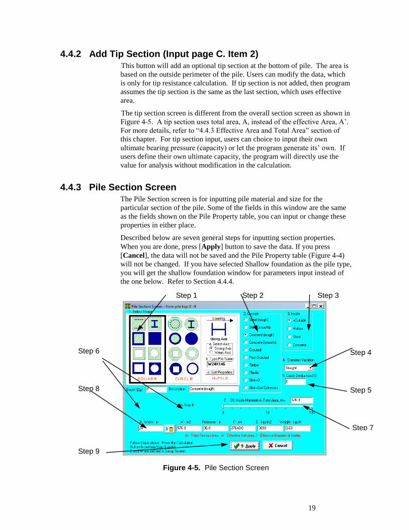
4.4.3 Pile Section Screen The Pile Section screen is for inputting pile material and size for the
particular section of the pile. Some of the fields in this window are the same
as the fields shown on the Pile Property table, you can input or change these
properties in either place.
Described below are seven general steps for inputting section properties.
When you are done, press [Apply] button to save the data. If you press
[Cancel], the data will not be saved and the Pile Property table (Figure 4-4)
will not be changed. If you have selected Shallow foundation as the pile type,
you will get the shallow foundation window for parameters input instead of
the one below. Refer to Section 4.4.4.
Figure 4-5. Pile Section Screen
Step 1 Step 2 Step 3
Step 4
Step 5
Step 7
Step 6
Step 8
Step 9
20
. . . . . . . . .
Step 1 . Select Pile Shape
The shape of the pile can be square/rectangular, circular/octangular, or H-
shaped. The internal configuration of the pile can be solid (one material),
hollow (square or circular space inside), or different material on the skin than
on the inside.
If you select H-pile, you can also input the pile designation, such as W24X94.
Then select strong or weak axis (used for lateral analysis). Strong axis means
the lateral load is acting in the same direction as the pile axis (X-X). Next,
press [Get Properties] and the program will search the database and get the
corresponding properties for the H-pile. If no match is found, the program
will select the closest size pile or give a warning message.
Step 2. Select Outside Skin Materials
Select the outside skin material from the materials list. Skin material affects
the result for vertical analysis. The parameter of each material can be modify
in setup screen. The E of the outside materials are used for E input.
Steel-Rough Specially treated rough surface
Steel-Smooth Steel pipe or H-pile with normal surface
Concrete-Rough Concrete cast directly against the soil such as auger-
cast piles
Concrete-Smooth Concrete cast in steel casing with smooth surface or
pre-cast concrete pile
Grouted Cement with high grouting pressure during
installation such as tie-back anchor or micro pile
Post-Grouted Grouting twice or more with higher grouting
pressure
Timber (Tapered) Timber pile with large top and smaller tip (users
should define the start depth and the start diameter,
then the end depth and the end diameter)
Plastic Pile with plastic surface
No-friction Steel No friction, or frictionless part of pile, such as the
unbound length of tieback anchor
Sf = Soil Cohesion The ultimate side resistance (adhesion) equals to soil
cohesion. Users can directly input C as adhesion in
Input Page E.
Step 3. Select Inside Materials
The inside of the pile can be:
= Outside The same material as the outside skin
Hollow No material inside
Steel Reinforcement bar in concrete
Concrete Steel pipe filled with concrete
21
. . . . . . . . .
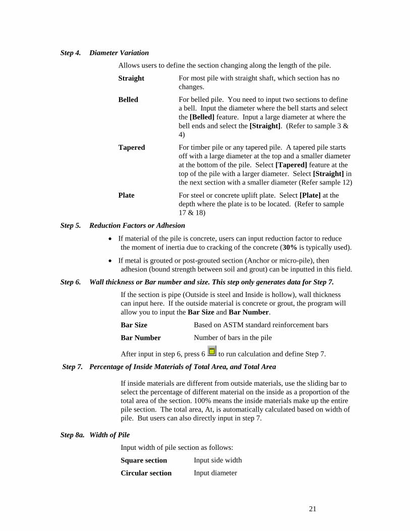
Step 4. Diameter Variation
Allows users to define the section changing along the length of the pile.
Straight For most pile with straight shaft, which section has no
changes.
Belled For belled pile. You need to input two sections to define
a bell. Input the diameter where the bell starts and select
the [Belled] feature. Input a large diameter at where the
bell ends and select the [Straight]. (Refer to sample 3 &
4)
Tapered For timber pile or any tapered pile. A tapered pile starts
off with a large diameter at the top and a smaller diameter
at the bottom of the pile. Select [Tapered] feature at the
top of the pile with a larger diameter. Select [Straight] in
the next section with a smaller diameter (Refer sample 12)
Plate For steel or concrete uplift plate. Select [Plate] at the
depth where the plate is to be located. (Refer to sample
17 & 18)
Step 5. Reduction Factors or Adhesion
If material of the pile is concrete, users can input reduction factor to reduce
the moment of inertia due to cracking of the concrete (30% is typically used).
If metal is grouted or post-grouted section (Anchor or micro-pile), then
adhesion (bound strength between soil and grout) can be inputted in this field.
Step 6. Wall thickness or Bar number and size. This step only generates data for Step 7.
If the section is pipe (Outside is steel and Inside is hollow), wall thickness
can input here. If the outside material is concrete or grout, the program will
allow you to input the Bar Size and Bar Number.
Bar Size Based on ASTM standard reinforcement bars
Bar Number Number of bars in the pile
After input in step 6, press 6 to run calculation and define Step 7.
Step 7. Percentage of Inside Materials of Total Area, and Total Area
If inside materials are different from outside materials, use the sliding bar to
select the percentage of different material on the inside as a proportion of the
total area of the section. 100% means the inside materials make up the entire
pile section. The total area, At, is automatically calculated based on width of
pile. But users can also directly input in step 7.
Step 8a. Width of Pile
Input width of pile section as follows:
Square section Input side width
Circular section Input diameter
22
. . . . . . . . .
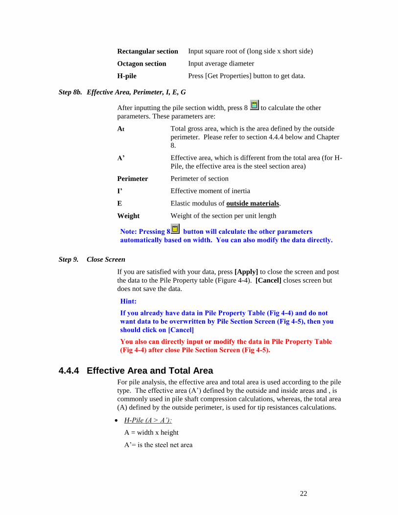
Rectangular section Input square root of (long side x short side)
Octagon section Input average diameter
H-pile Press [Get Properties] button to get data.
Step 8b. Effective Area, Perimeter, I, E, G
After inputting the pile section width, press 8 to calculate the other
parameters. These parameters are:
At Total gross area, which is the area defined by the outside
perimeter. Please refer to section 4.4.4 below and Chapter
8.
A’ Effective area, which is different from the total area (for H-
Pile, the effective area is the steel section area)
Perimeter Perimeter of section
I’ Effective moment of inertia
E Elastic modulus of outside materials.
Weight Weight of the section per unit length
Note: Pressing 8 button will calculate the other parameters
automatically based on width. You can also modify the data directly.
Step 9. Close Screen
If you are satisfied with your data, press [Apply] to close the screen and post
the data to the Pile Property table (Figure 4-4). [Cancel] closes screen but
does not save the data.
Hint:
If you already have data in Pile Property Table (Fig 4-4) and do not
want data to be overwritten by Pile Section Screen (Fig 4-5), then you
should click on [Cancel]
You also can directly input or modify the data in Pile Property Table
(Fig 4-4) after close Pile Section Screen (Fig 4-5).
4.4.4 Effective Area and Total Area For pile analysis, the effective area and total area is used according to the pile
type. The effective area (A’) defined by the outside and inside areas and , is
commonly used in pile shaft compression calculations, whereas, the total area
(A) defined by the outside perimeter, is used for tip resistances calculations.
H-Pile (A > A’):
A = width x height
A’= is the steel net area
23
. . . . . . . . .
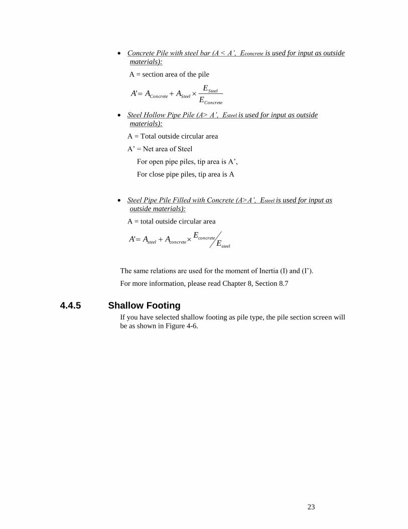
Concrete Pile with steel bar (A < A’, Econcrete is used for input as outside
materials):
A = section area of the pile
Concrete
Steel
SteelConcreteE
EAAA '
Steel Hollow Pipe Pile (A> A’, Esteel is used for input as outside
materials):
A = Total outside circular area
A’ = Net area of Steel
For open pipe piles, tip area is A’,
For close pipe piles, tip area is A
Steel Pipe Pile Filled with Concrete (A>A’, Esteel is used for input as
outside materials):
A = total outside circular area
steel
concreteconcretesteel E
EAAA '
The same relations are used for the moment of Inertia (I) and (I’).
For more information, please read Chapter 8, Section 8.7
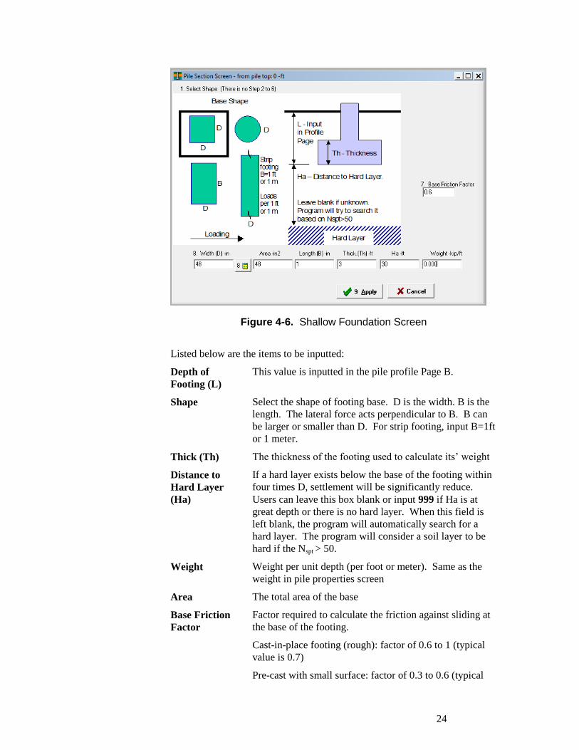
4.4.5 Shallow Footing If you have selected shallow footing as pile type, the pile section screen will
be as shown in Figure 4-6.
24
. . . . . . . . .
Listed below are the items to be inputted:
Depth of
Footing (L)
This value is inputted in the pile profile Page B.
Shape Select the shape of footing base. D is the width. B is the
length. The lateral force acts perpendicular to B. B can
be larger or smaller than D. For strip footing, input B=1ft
or 1 meter.
Thick (Th) The thickness of the footing used to calculate its’ weight
Distance to
Hard Layer
(Ha)
If a hard layer exists below the base of the footing within
four times D, settlement will be significantly reduce.
Users can leave this box blank or input 999 if Ha is at
great depth or there is no hard layer. When this field is
left blank, the program will automatically search for a
hard layer. The program will consider a soil layer to be
hard if the Nspt > 50.
Weight Weight per unit depth (per foot or meter). Same as the
weight in pile properties screen
Area The total area of the base
Base Friction
Factor
Factor required to calculate the friction against sliding at
the base of the footing.
Cast-in-place footing (rough): factor of 0.6 to 1 (typical
value is 0.7)
Pre-cast with small surface: factor of 0.3 to 0.6 (typical
Figure 4-6. Shallow Foundation Screen
25
. . . . . . . . .
value 0.4 is used)
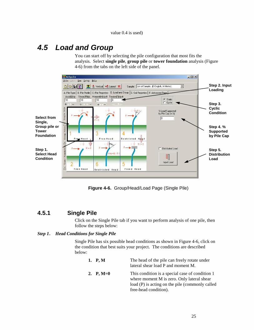
4.5 Load and Group You can start off by selecting the pile configuration that most fits the
analysis. Select single pile, group pile or tower foundation analysis (Figure
4-6) from the tabs on the left side of the panel.
4.5.1 Single Pile Click on the Single Pile tab if you want to perform analysis of one pile, then
follow the steps below:
Step 1 . Head Conditions for Single Pile
Single Pile has six possible head conditions as shown in Figure 4-6, click on
the condition that best suits your project. The conditions are described
below:
1. P, M The head of the pile can freely rotate under
lateral shear load P and moment M.
2. P, M=0 This condition is a special case of condition 1
where moment M is zero. Only lateral shear
load (P) is acting on the pile (commonly called
free-head condition).
Figure 4-6. Group/Head/Load Page (Single Pile)
Select from
Single,
Group pile or
Tower
Foundation
Step 1.
Select Head
Condition
Step 2. Input
Loading
Step 3.
Cyclic
Condition
Step 4. %
Supported
by Pile Cap
Step 5.
Distribution
Load
26
. . . . . . . . .
3. P=0, M Shear load is zero and only moment is acting on
the pile top, a special case of condition 1.
4. P, St St is the top rotation in degrees. Input St to
force the pile head to rotate to a certain degree.
5. P, St=0 Commonly called fixed-head, there is no
rotation in the pile head, since St=0. Moment
will be generated at the pile head.
6. P, Kms Kms is head rotation stiffness in moment per
unit slope (useful for some structural analyses).
Input Kt along with P. If Kms=0, then it is the
same as condition 2 above (P, M=0).
NOTE: All the conditions can be combined with vertical load (Q).
Step 2. Load Conditions for Single Pile
Based on the head conditions, there are many combinations of loads. The
program automatically selects load combinations based on the head condition
selected. Possible loads are:
Vertical load (Q) – Downward and uplift working load at pile top. Input a
negative value for uplift load. The program will calculate both downward and
uplift capacity in the vertical analysis. For batter pile, Q is axial load.
Shear load (P) – Lateral working load at pile top. Positive value of P is from
left to right, and negative value is from right to left.
Moment (M) – Working moment on the pile head. A positive value if M is
clockwise and a negative value if M is counterclockwise.
Torsion (T) – Torsion generated at the pile cap. Twisting of the pile cap due
to external load.
Slope (St) – The known slope angle at the pile head. Negative value is
clockwise and positive value is counterclockwise (unit is deflection/length).
Stiffness (Kms or Kt) – The rotation stiffness Kms or Kt is the ratio of
moment/slope (M/St). Negative value is clockwise and positive value is
counterclockwise (unit is the same as M).
Step 3 Cyclic Conditions
Select Static or Cyclic shear load. If the load is cyclic, specify the number of
cycles in the No. of Cycles box (between 2 and 500).
NOTE: The cyclic condition only applies to lateral analysis, not vertical.
Step 4 Percentage Load Supported by Pile Cap
You can adjust the amount of vertical load carried by the pile cap. For 0%
load supported by the pile cap, the entire load is transfer to the pile therefore
27
. . . . . . . . .
dissipated by the pile at greater depth. For 100% load supported, the entire
load is supported by the pile cap.
Note: To be conservation using 0% is recommended.
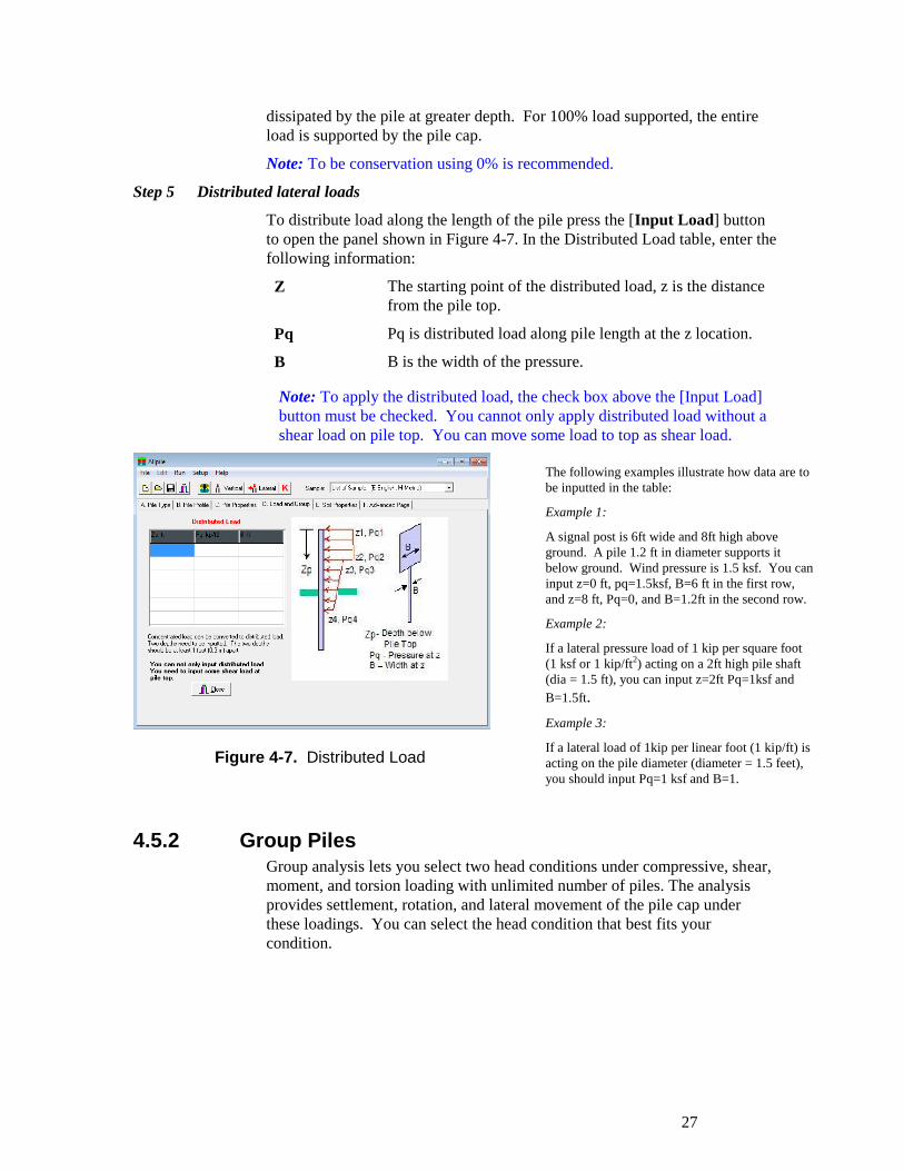
Step 5 Distributed lateral loads
To distribute load along the length of the pile press the [Input Load] button
to open the panel shown in Figure 4-7. In the Distributed Load table, enter the
following information:
Z The starting point of the distributed load, z is the distance
from the pile top.
Pq Pq is distributed load along pile length at the z location.
B B is the width of the pressure.
4.5.2 Group Piles Group analysis lets you select two head conditions under compressive, shear,
moment, and torsion loading with unlimited number of piles. The analysis
provides settlement, rotation, and lateral movement of the pile cap under
these loadings. You can select the head condition that best fits your
condition.
The following examples illustrate how data are to
be inputted in the table:
Example 1:
A signal post is 6ft wide and 8ft high above
ground. A pile 1.2 ft in diameter supports it
below ground. Wind pressure is 1.5 ksf. You can
input z=0 ft, pq=1.5ksf, B=6 ft in the first row,
and z=8 ft, Pq=0, and B=1.2ft in the second row.
Example 2:
If a lateral pressure load of 1 kip per square foot
(1 ksf or 1 kip/ft2) acting on a 2ft high pile shaft
(dia = 1.5 ft), you can input z=2ft Pq=1ksf and
B=1.5ft.
Example 3:
If a lateral load of 1kip per linear foot (1 kip/ft) is
acting on the pile diameter (diameter = 1.5 feet),
you should input Pq=1 ksf and B=1.
Figure 4-7. Distributed Load
Note: To apply the distributed load, the check box above the [Input Load]
button must be checked. You cannot only apply distributed load without a
shear load on pile top. You can move some load to top as shear load.
28
. . . . . . . . .
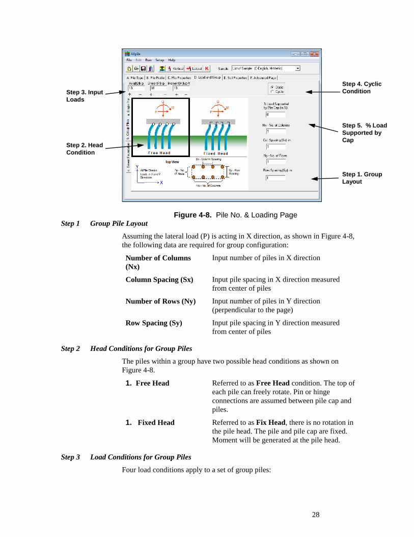
Step 1 Group Pile Layout
Assuming the lateral load (P) is acting in X direction, as shown in Figure 4-8,
the following data are required for group configuration:
Number of Columns
(Nx)
Input number of piles in X direction
Column Spacing (Sx) Input pile spacing in X direction measured
from center of piles
Number of Rows (Ny) Input number of piles in Y direction
(perpendicular to the page)
Row Spacing (Sy) Input pile spacing in Y direction measured
from center of piles
Step 2 Head Conditions for Group Piles
The piles within a group have two possible head conditions as shown on
Figure 4-8.
1. Free Head Referred to as Free Head condition. The top of
each pile can freely rotate. Pin or hinge
connections are assumed between pile cap and
piles.
1. Fixed Head Referred to as Fix Head, there is no rotation in
the pile head. The pile and pile cap are fixed.
Moment will be generated at the pile head.
Step 3 Load Conditions for Group Piles
Four load conditions apply to a set of group piles:
Figure 4-8. Pile No. & Loading Page
Step 4. Cyclic
Condition
Step 5. % Load
Supported by
Cap
Step 1. Group
Layout
Step 3. Input
Loads
Step 2. Head
Condition
29
. . . . . . . . .
Vertical load (Q) – Downward and uplift working load at pile cap, equally
distributed to all piles in the group. Input a negative value for uplift load.
Lateral load (P) – Lateral working load at pile cap. Positive value of P is
from left to right, and negative value is from right to left. Load will be
distributed to all piles in the group based on their lateral stiffness.
Moment (M) – Moment generated at the pile cap. Positive value of P is
clockwise and a negative value is counterclockwise. There are no moments
at the tip of each pile individually due to the fixation of head by the pile cap.
Step 4 Cyclic Conditions
Select Static or Cyclic shear load. No. of Cycles (between 2 and 500). Only
for lateral analysis
Step 5 Percentage of Load Supported by Pile Cap
You can adjust the amount of vertical load carried by the pile cap. For 0%
load supported by the pile cap, the entire load is transfer to the pile therefore
dissipated by the pile at greater depth. For 100% load supported, the pile cap
supports the entire load.
Note: To be conservative using 0% is recommended.
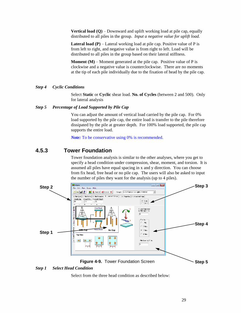
4.5.3 Tower Foundation Tower foundation analysis is similar to the other analyses, where you get to
specify a head condition under compression, shear, moment, and torsion. It is
assumed all piles have equal spacing in x and y direction. You can choose
from fix head, free head or no pile cap. The users will also be asked to input
the number of piles they want for the analysis (up to 4 piles).
Step 1 Select Head Condition
Select from the three head condition as described below:
Figure 4-9. Tower Foundation Screen
Step 2
Step 1
Step 3
Step 4
Step 5
30
. . . . . . . . .
Free Head Top of the pile can freely rotate. Pin or hinge
connections are assumed between pile caps and piles.
Fixed Head There are no rotation in the pile cap. Piles and pile cap
are fixed. Moment will be generated at the pile head.
No Cap There is no pile cap to connect each pile.
Step 2 Load Conditions for Group Piles
Four load conditions apply to a set of group piles:
Vertical load (Q) – Downward and uplift working load at pile cap, equally
distributed to all piles in the group. Input a negative value for uplift load.
Shear load (P) – Lateral working load at pile cap. Positive value of P is from
left to right, and negative value is from right to left. Load will be distributed
to all piles in the group based on their lateral stiffness.
Moment (M) – Moment generated at the pile cap. Positive value of P is
clockwise and a negative value is counterclockwise. There are no moments
at the tip of each pile individually due to the fixation of head by the pile cap.
Step3 Cyclic Conditions
Select Static or Cyclic shear load. No. of Cycles (between 2 and 500). This
information is for lateral analyses only.
Step 4 Pile Number
The total number of piles under a tower.
Step 5 Pile Spacing
The spacing between piles are assumed to be equal. Spacing has to be input
in inches or cm. It is assumed x and y direction have the same spacing.
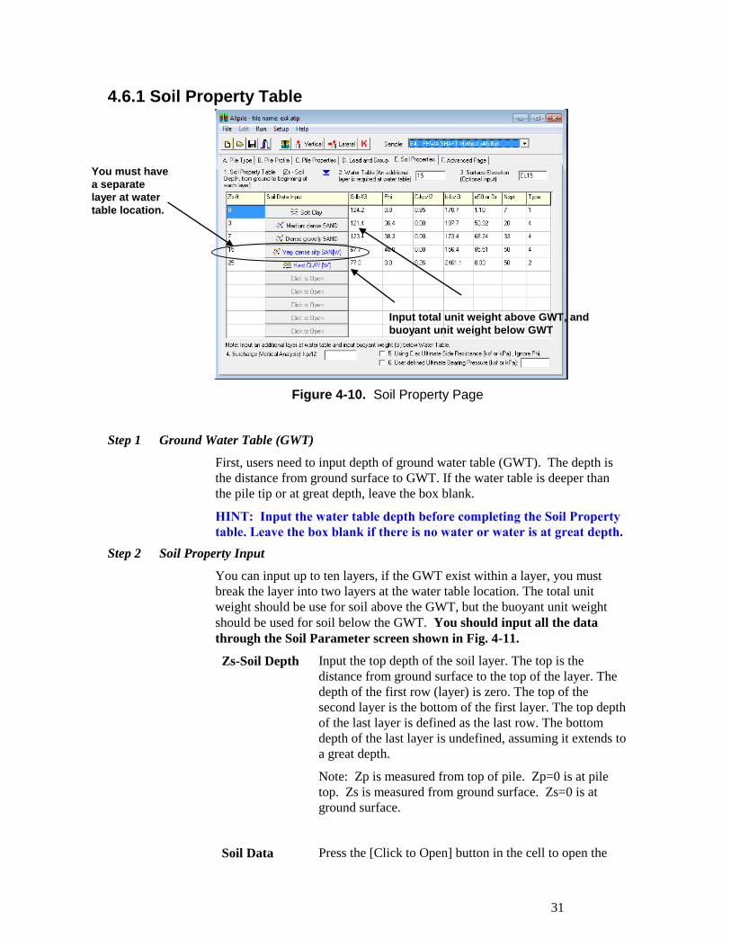
4.6 Soil Property Page The Soil Property page (Figure 4-10) allows you to input water and soil
information in four easy steps.
31
. . . . . . . . .
4.6.1 Soil Property Table
Step 1 Ground Water Table (GWT)
First, users need to input depth of ground water table (GWT). The depth is
the distance from ground surface to GWT. If the water table is deeper than
the pile tip or at great depth, leave the box blank.
HINT: Input the water table depth before completing the Soil Property
table. Leave the box blank if there is no water or water is at great depth.
Step 2 Soil Property Input
You can input up to ten layers, if the GWT exist within a layer, you must
break the layer into two layers at the water table location. The total unit
weight should be use for soil above the GWT, but the buoyant unit weight
should be used for soil below the GWT. You should input all the data
through the Soil Parameter screen shown in Fig. 4-11.
Zs-Soil Depth Input the top depth of the soil layer. The top is the
distance from ground surface to the top of the layer. The
depth of the first row (layer) is zero. The top of the
second layer is the bottom of the first layer. The top depth
of the last layer is defined as the last row. The bottom
depth of the last layer is undefined, assuming it extends to
a great depth.
Note: Zp is measured from top of pile. Zp=0 is at pile
top. Zs is measured from ground surface. Zs=0 is at
ground surface.
Soil Data Press the [Click to Open] button in the cell to open the
Figure 4-10. Soil Property Page
You must have
a separate
layer at water
table location.
Input total unit weight above GWT, and
buoyant unit weight below GWT
32
. . . . . . . . .
Input Soil Parameter screen (see next section).
HINT: It is recommended to input all soil parameters
to the Soil Parameters screen (Figure 4-11).
G Unit weight of soil. If the soil is under the water table,
buoyant weight must be input. (This is why it is necessary
to divide a layer into two if the GWT sits within this
layer.) Buoyant weight is the total unit weight of the soil
minus the unit weight of the water.
HINT: Input total unit weight above GWT and
buoyant weight below GWT.
Phi Friction angle of soil.
C Cohesion of soil.
K Modulus of Subgrade Reaction of soil (for lateral analysis
only). If you only run vertical analysis, you don’t have to
input this value (Refer to Ch.8 for description).
e50 or Dr
If soil is silt, rock, or clay, e50 is strain at 50% deflection
in p-y curve (only used for cohesive soil in lateral
analysis) (Refer to Ch.8). If soil is sand, Dr is the relative
density from 0 to 100 (%). It is for reference only and is
not used in the analysis.
Nspt Standard Penetration Test (SPT) or N value, the number
of blows to penetrate 12 inches in soil (304.8 mm) with a
140-lb (622.72 N) hammer dropping a distance of 30
inches (0.762 m). Corrected SPT (N1) should be used. If
you do not have N1, use SPT instead.
Type Number of Soil Type defined in Soil Parameter screen
HINT: for more detail on k and e50, refer to Chapter 8, Lateral Analysis.
Step 3 Surface Elevation
It is optional to input a value in this field. If an elevation is inputted, the
depth of the pile is shown on the left side and the elevation is shown on the
right side of the chart.
33
. . . . . . . . .
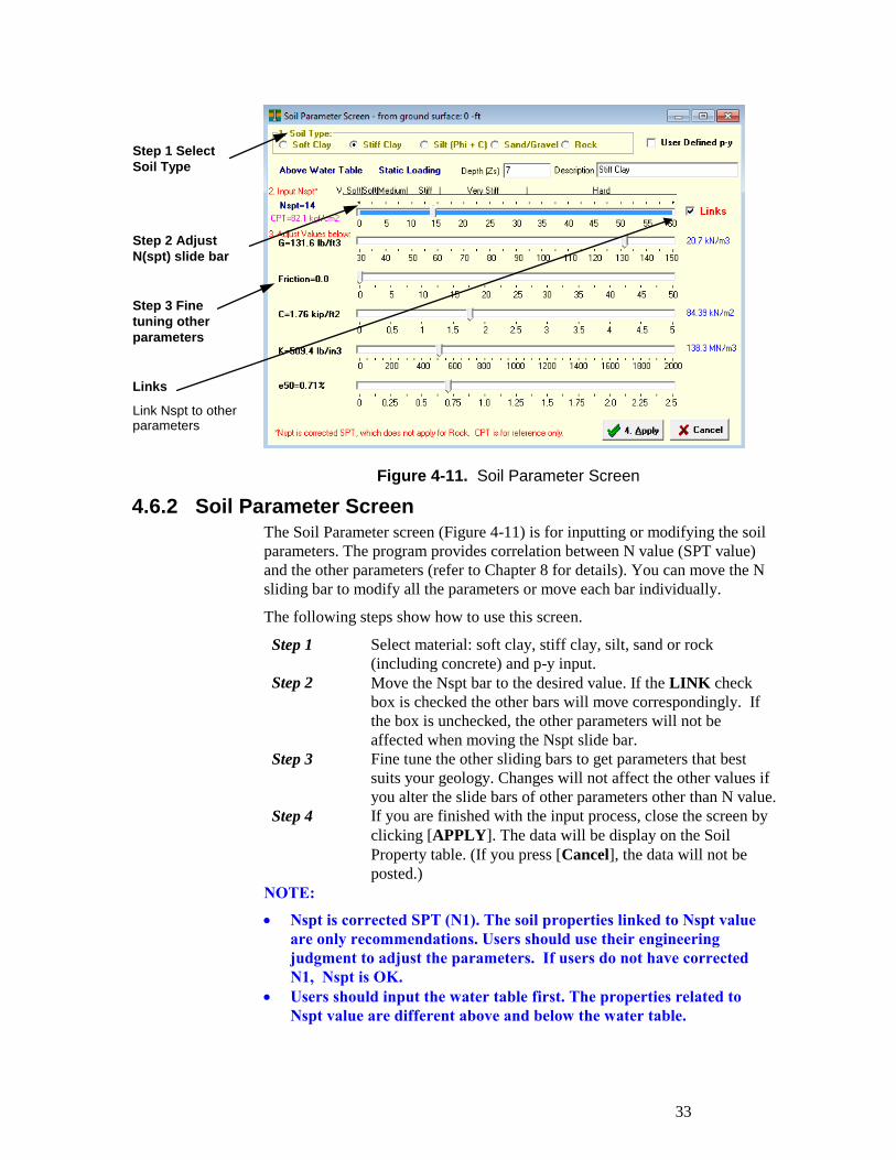
4.6.2 Soil Parameter Screen The Soil Parameter screen (Figure 4-11) is for inputting or modifying the soil
parameters. The program provides correlation between N value (SPT value)
and the other parameters (refer to Chapter 8 for details). You can move the N
sliding bar to modify all the parameters or move each bar individually.
The following steps show how to use this screen.
Step 1 Select material: soft clay, stiff clay, silt, sand or rock
(including concrete) and p-y input.
Step 2 Move the Nspt bar to the desired value. If the LINK check
box is checked the other bars will move correspondingly. If
the box is unchecked, the other parameters will not be
affected when moving the Nspt slide bar.
Step 3 Fine tune the other sliding bars to get parameters that best
suits your geology. Changes will not affect the other values if
you alter the slide bars of other parameters other than N value.
Step 4 If you are finished with the input process, close the screen by
clicking [APPLY]. The data will be display on the Soil
Property table. (If you press [Cancel], the data will not be
posted.)
NOTE:
Nspt is corrected SPT (N1). The soil properties linked to Nspt value
are only recommendations. Users should use their engineering
judgment to adjust the parameters. If users do not have corrected
N1, Nspt is OK.
Users should input the water table first. The properties related to
Nspt value are different above and below the water table.
Figure 4-11. Soil Parameter Screen
Step 1 Select
Soil Type
Step 2 Adjust
N(spt) slide bar
Step 3 Fine
tuning other
parameters
Links
Link Nspt to other parameters
34
. . . . . . . . .
If the users have a known properties (for example, C=5 ksf), users
can move N bar until the known properties reaches its value (In the
example, let C reach to 5 ksf).
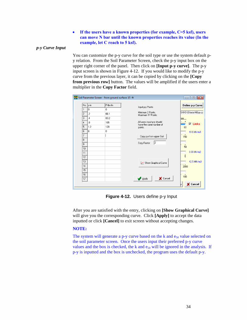
p-y Curve Input
You can customize the p-y curve for the soil type or use the system default p-
y relation. From the Soil Parameter Screen, check the p-y input box on the
upper right corner of the panel. Then click on [Input p-y curve]. The p-y
input screen is shown in Figure 4-12. If you would like to modify the p-y
curve from the previous layer, it can be copied by clicking on the [Copy
from previous row] button. The values will be amplified if the users enter a
multiplier in the Copy Factor field.
After you are satisfied with the entry, clicking on [Show Graphical Curve]
will give you the corresponding curve. Click [Apply] to accept the data
inputted or click [Cancel] to exit screen without accepting changes.
NOTE:
The system will generate a p-y curve based on the k and e50 value selected on
the soil parameter screen. Once the users input their preferred p-y curve
values and the box is checked, the k and e50 will be ignored in the analysis. If
p-y is inputted and the box is unchecked, the program uses the default p-y.
Figure 4-12. Users define p-y Input
35
. . . . . . . . .
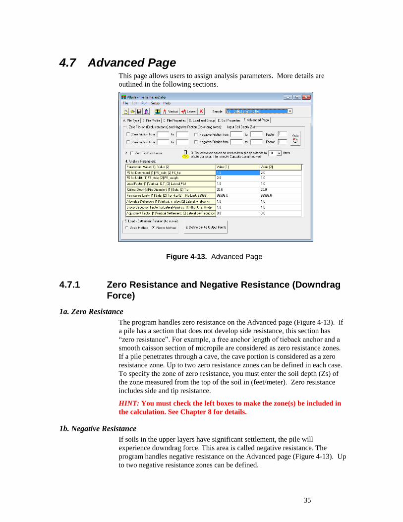
4.7 Advanced Page This page allows users to assign analysis parameters. More details are
outlined in the following sections.
4.7.1 Zero Resistance and Negative Resistance (Downdrag
Force)
1a. Zero Resistance
The program handles zero resistance on the Advanced page (Figure 4-13). If
a pile has a section that does not develop side resistance, this section has
“zero resistance”. For example, a free anchor length of tieback anchor and a
smooth caisson section of micropile are considered as zero resistance zones.
If a pile penetrates through a cave, the cave portion is considered as a zero
resistance zone. Up to two zero resistance zones can be defined in each case.
To specify the zone of zero resistance, you must enter the soil depth (Zs) of
the zone measured from the top of the soil in (feet/meter). Zero resistance
includes side and tip resistance.
HINT: You must check the left boxes to make the zone(s) be included in
the calculation. See Chapter 8 for details.
1b. Negative Resistance
If soils in the upper layers have significant settlement, the pile will
experience downdrag force. This area is called negative resistance. The
program handles negative resistance on the Advanced page (Figure 4-13). Up
to two negative resistance zones can be defined.
Figure 4-13. Advanced Page
36
. . . . . . . . .
“Factor” is the effective factor, Kneg. It ranges from 0 to 1 depending on the
impact of soil settlement on the pile shaft. If the factor equals 1, then the
negative friction is equal to the friction in the downward capacity analysis. If
the factor equals 0, then there is no friction between pile and soils. It is the
same as zero friction. If the pile has a smooth surface and the soil has small
settlement, Kneg is in the range of 0 to 0.3. If the pile has a rough surface and
the soil has a large settlement, Kneg is 0.3 to 0.6.
HINTS:
1. If Kneg = 0, there is no resistance between the pile and the soil, i.e., it
is the same as zero resistance.
2. Kneg should be a positive value rather than using a negative value.
3. You must check the check box on the left side so that the calculation
will take into account the negative resistance.
4. The negative resistance only applies to downward side resistance, not
tip resistance. The induced downdrag force reduces the pile capacity
in the analysis.
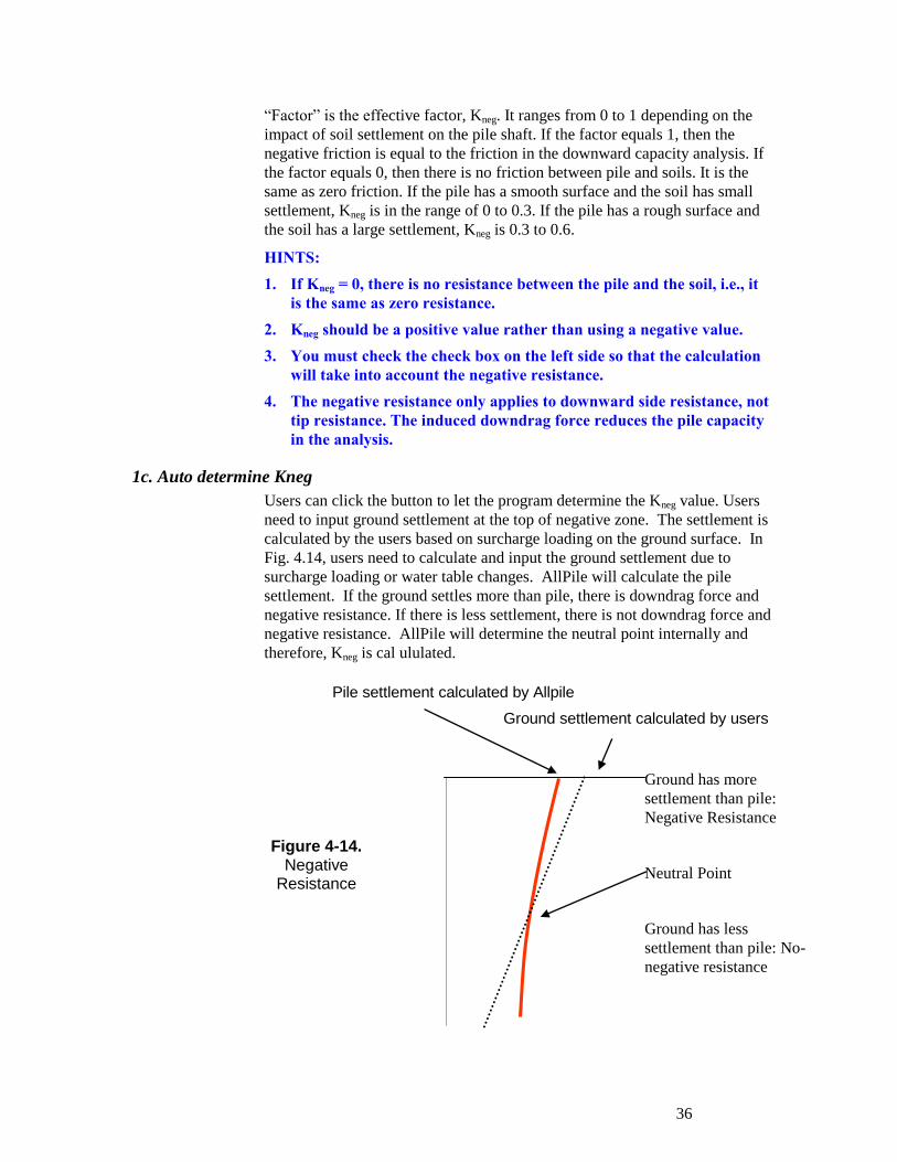
1c. Auto determine Kneg
Users can click the button to let the program determine the Kneg value. Users
need to input ground settlement at the top of negative zone. The settlement is
calculated by the users based on surcharge loading on the ground surface. In
Fig. 4.14, users need to calculate and input the ground settlement due to
surcharge loading or water table changes. AllPile will calculate the pile
settlement. If the ground settles more than pile, there is downdrag force and
negative resistance. If there is less settlement, there is not downdrag force and
negative resistance. AllPile will determine the neutral point internally and
therefore, Kneg is cal ululated.
Pile settlement calculated by Allpile
Ground settlement calculated by users
Ground has more
settlement than pile:
Negative Resistance
Neutral Point
Ground has less
settlement than pile: No-
negative resistance
Figure 4-14. Negative
Resistance
37
. . . . . . . . .
2. Zero Tip Resistance
If users do not want the tip resistance included in the vertical capacity, this box
can be checked.
3. Define Tip Stratum
Tip resistance calculation is based on the soil properties at pile tip. There may
be several very thin layers under the tip. If the stratum is not defined (as zero),
the first layer below the tip will control the results. Users should define a
stratum thick enough to include all the influence layers. 10 times pile diameter
is recommended. This will provide more reasonable results and also smooth the
pile capacity vs. pile length curve. For shallow footing, 4 times footing width is
recommended. If a hard stratum is defined in footing property screen, the Tip
Stratum is limited to the hard stratum.
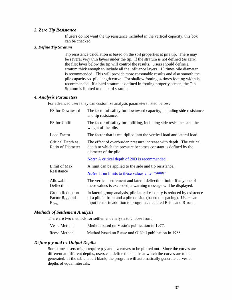
4. Analysis Parameters
For advanced users they can customize analysis parameters listed below:
FS for Downward The factor of safety for downward capacity, including side resistance
and tip resistance.
FS for Uplift The factor of safety for uplifting, including side resistance and the
weight of the pile.
Load Factor The factor that is multiplied into the vertical load and lateral load.
Critical Depth as
Ratio of Diameter
The effect of overburden pressure increase with depth. The critical
depth to which the pressure becomes constant is defined by the
diameter of the pile.
Note: A critical depth of 20D is recommended
Limit of Max
Resistance
A limit can be applied to the side and tip resistance.
Note: If no limits to these values enter “9999”
Allowable
Deflection
The vertical settlement and lateral deflection limit. If any one of
these values is exceeded, a warning message will be displayed.
Group Reduction
Factor Rside and
Rfront
In lateral group analysis, pile lateral capacity is reduced by existence
of a pile in front and a pile on side (based on spacing). Users can
input factor in addition to program calculated Rside and Rfront.
Methods of Settlement Analysis
There are two methods for settlement analysis to choose from.
Vesic Method Method based on Vesic’s publication in 1977.
Reese Method Method based on Reese and O’Neil publication in 1988.
Define p-y and t-z Output Depths
Sometimes users might require p-y and t-z curves to be plotted out. Since the curves are
different at different depths, users can define the depths at which the curves are to be
generated. If the table is left blank, the program will automatically generate curves at
depths of equal intervals.
38
. . . . . . . . .
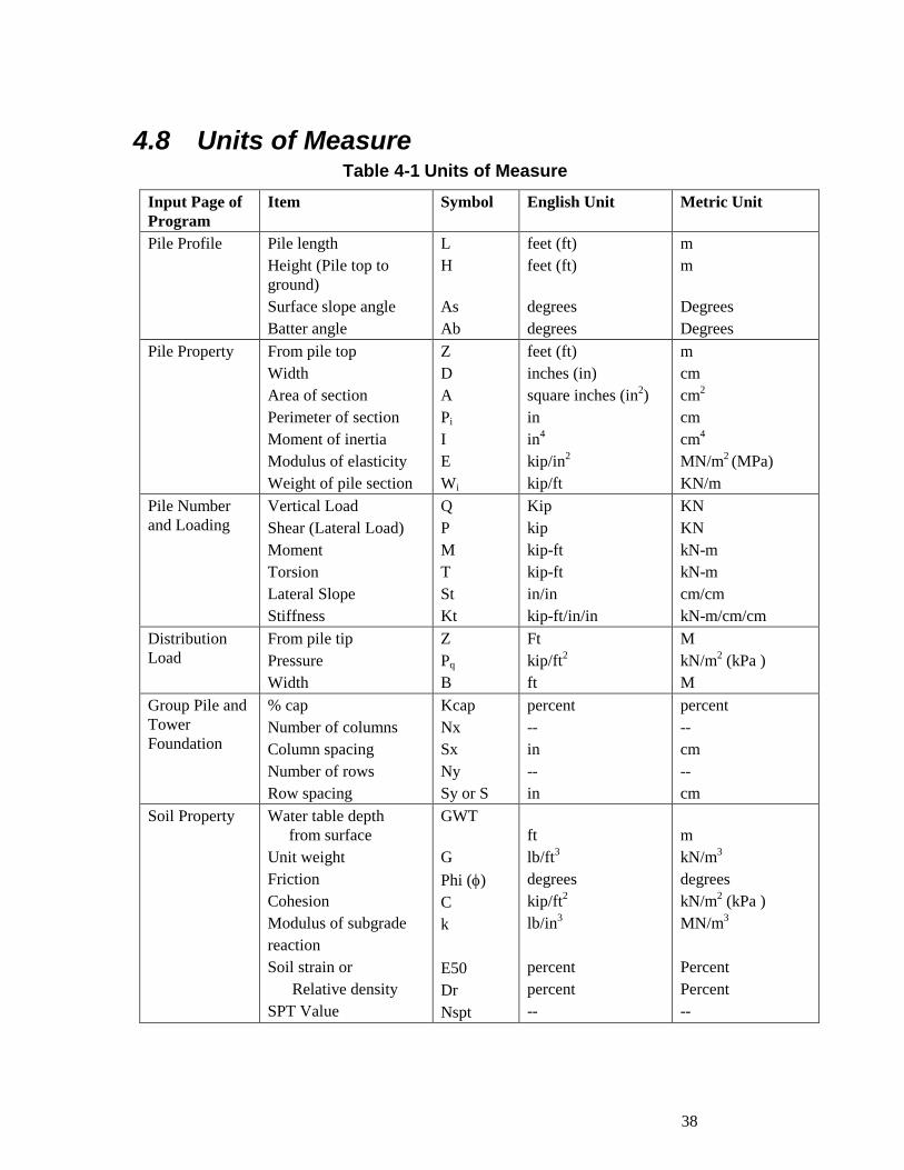
4.8 Units of Measure Table 4-1 Units of Measure
Input Page of
Program
Item Symbol English Unit Metric Unit
Pile Profile Pile length
Height (Pile top to
ground)
Surface slope angle
Batter angle
L
H
As
Ab
feet (ft)
feet (ft)
degrees
degrees
m
m
Degrees
Degrees
Pile Property From pile top
Width
Area of section
Perimeter of section
Moment of inertia
Modulus of elasticity
Weight of pile section
Z
D
A
Pi
I
E
Wi
feet (ft)
inches (in)
square inches (in2)
in
in4
kip/in2
kip/ft
m
cm
cm2
cm
cm4
MN/m2 (MPa)
KN/m
Pile Number
and Loading
Vertical Load
Shear (Lateral Load)
Moment
Torsion
Lateral Slope
Stiffness
Q
P
M
T
St
Kt
Kip
kip
kip-ft
kip-ft
in/in
kip-ft/in/in
KN
KN
kN-m
kN-m
cm/cm
kN-m/cm/cm
Distribution
Load
From pile tip
Pressure
Width
Z
Pq
B
Ft
kip/ft2
ft
M
kN/m2 (kPa )
M
Group Pile and
Tower
Foundation
% cap
Number of columns
Column spacing
Number of rows
Row spacing
Kcap
Nx
Sx
Ny
Sy or S
percent
--
in
--
in
percent
--
cm
--
cm
Soil Property
Water table depth
from surface
Unit weight
Friction
Cohesion
Modulus of subgrade
reaction
Soil strain or
Relative density
SPT Value
GWT
G
Phi ()
C
k
E50
Dr
Nspt
ft
lb/ft3
degrees
kip/ft2
lb/in3
percent
percent
--
m
kN/m3
degrees
kN/m2 (kPa )
MN/m3
Percent
Percent
--
39
. . . . . . . . .
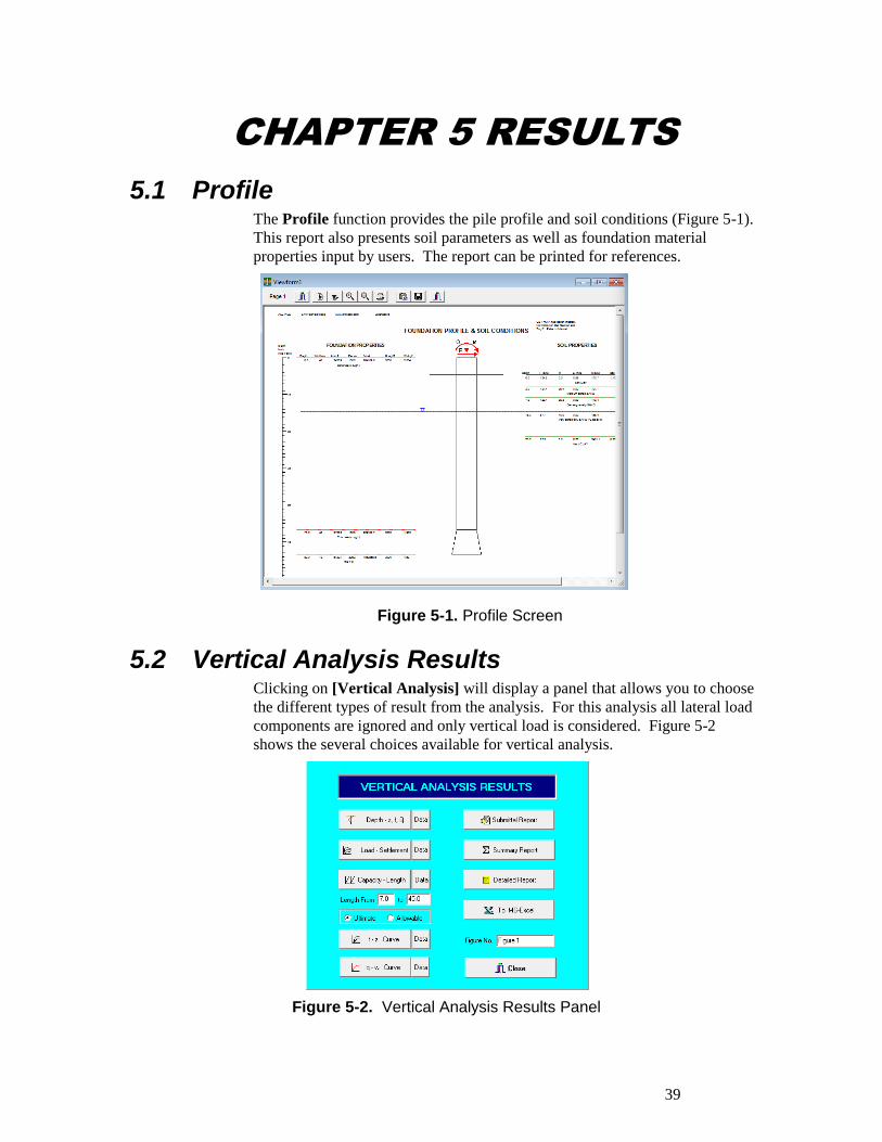
CHAPTER 5 RESULTS
5.1 Profile The Profile function provides the pile profile and soil conditions (Figure 5-1).
This report also presents soil parameters as well as foundation material
properties input by users. The report can be printed for references.
5.2 Vertical Analysis Results Clicking on [Vertical Analysis] will display a panel that allows you to choose
the different types of result from the analysis. For this analysis all lateral load
components are ignored and only vertical load is considered. Figure 5-2
shows the several choices available for vertical analysis.
Figure 5-2. Vertical Analysis Results Panel
Figure 5-1. Profile Screen
40
. . . . . . . . .
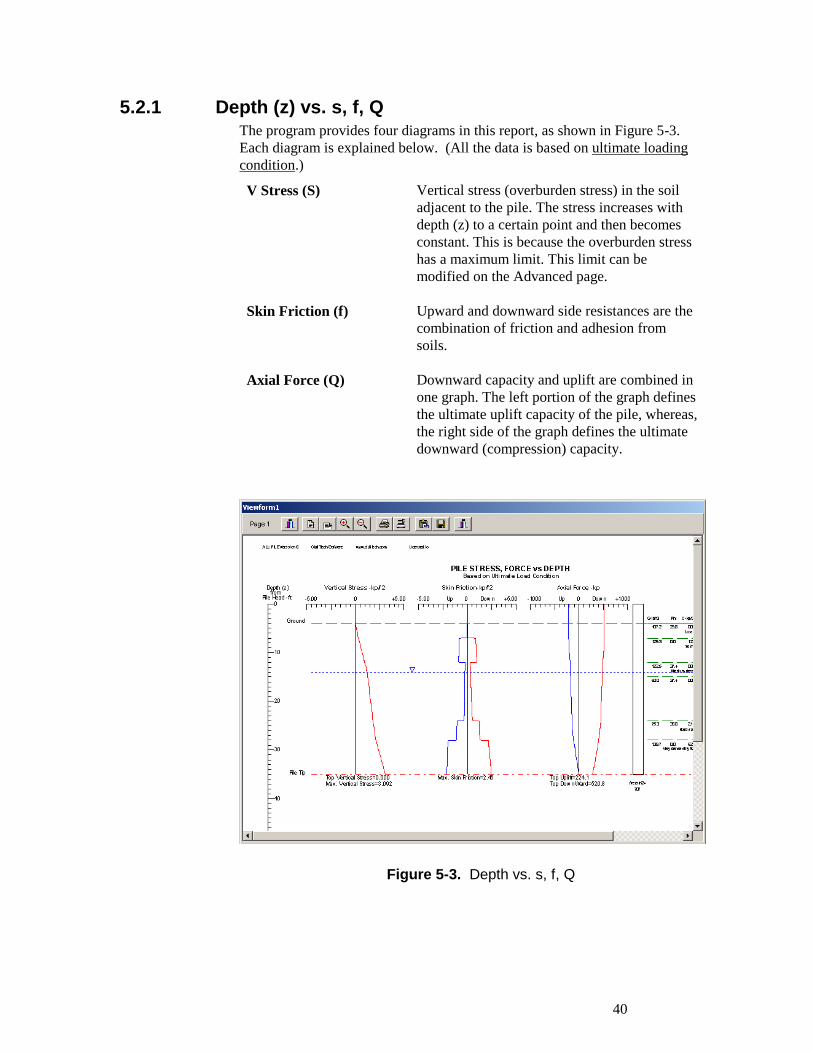
5.2.1 Depth (z) vs. s, f, Q The program provides four diagrams in this report, as shown in Figure 5-3.
Each diagram is explained below. (All the data is based on ultimate loading
condition.)
V Stress (S) Vertical stress (overburden stress) in the soil
adjacent to the pile. The stress increases with
depth (z) to a certain point and then becomes
constant. This is because the overburden stress
has a maximum limit. This limit can be
modified on the Advanced page.
Skin Friction (f) Upward and downward side resistances are the
combination of friction and adhesion from
soils.
Axial Force (Q) Downward capacity and uplift are combined in
one graph. The left portion of the graph defines
the ultimate uplift capacity of the pile, whereas,
the right side of the graph defines the ultimate
downward (compression) capacity.
Figure 5-3. Depth vs. s, f, Q
41
. . . . . . . . .
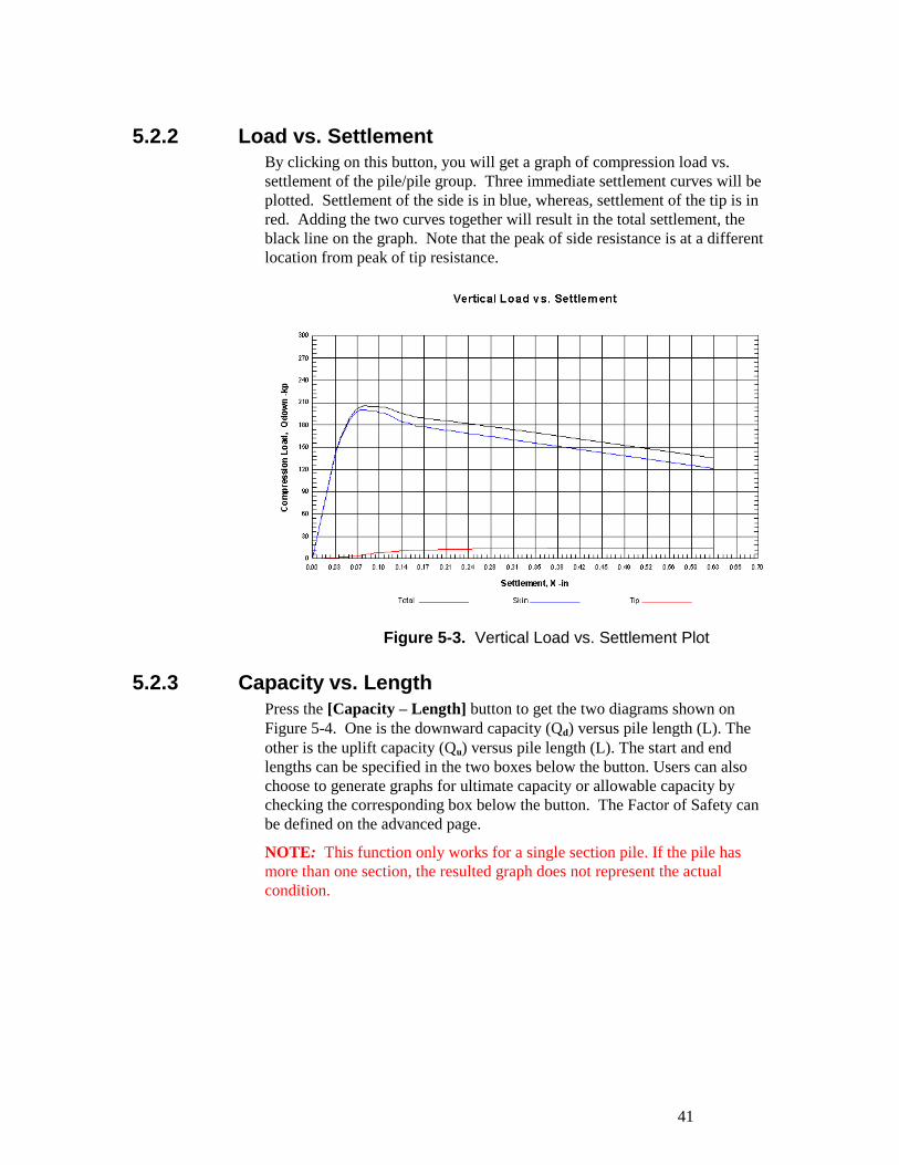
5.2.2 Load vs. Settlement By clicking on this button, you will get a graph of compression load vs.
settlement of the pile/pile group. Three immediate settlement curves will be
plotted. Settlement of the side is in blue, whereas, settlement of the tip is in
red. Adding the two curves together will result in the total settlement, the
black line on the graph. Note that the peak of side resistance is at a different
location from peak of tip resistance.
5.2.3 Capacity vs. Length
Press the [Capacity – Length] button to get the two diagrams shown on
Figure 5-4. One is the downward capacity (Qd) versus pile length (L). The
other is the uplift capacity (Qu) versus pile length (L). The start and end
lengths can be specified in the two boxes below the button. Users can also
choose to generate graphs for ultimate capacity or allowable capacity by
checking the corresponding box below the button. The Factor of Safety can
be defined on the advanced page.
NOTE: This function only works for a single section pile. If the pile has
more than one section, the resulted graph does not represent the actual
condition.
Figure 5-3. Vertical Load vs. Settlement Plot
42
. . . . . . . . .
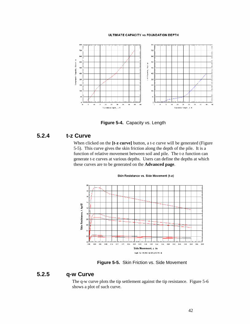
5.2.4 t-z Curve
When clicked on the [t-z curve] button, a t-z curve will be generated (Figure
5-5). This curve gives the skin friction along the depth of the pile. It is a
function of relative movement between soil and pile. The t-z function can
generate t-z curves at various depths. Users can define the depths at which
these curves are to be generated on the Advanced page.
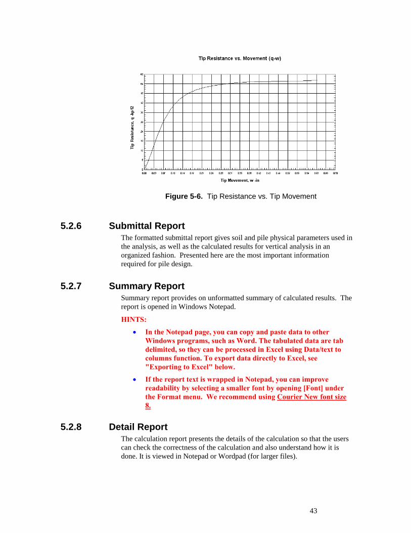
5.2.5 q-w Curve The q-w curve plots the tip settlement against the tip resistance. Figure 5-6
shows a plot of such curve.
Figure 5-4. Capacity vs. Length
Figure 5-5. Skin Friction vs. Side Movement
43
. . . . . . . . .
5.2.6 Submittal Report The formatted submittal report gives soil and pile physical parameters used in
the analysis, as well as the calculated results for vertical analysis in an
organized fashion. Presented here are the most important information
required for pile design.
5.2.7 Summary Report Summary report provides on unformatted summary of calculated results. The
report is opened in Windows Notepad.
HINTS:
In the Notepad page, you can copy and paste data to other
Windows programs, such as Word. The tabulated data are tab
delimited, so they can be processed in Excel using Data/text to
columns function. To export data directly to Excel, see
"Exporting to Excel" below.
If the report text is wrapped in Notepad, you can improve
readability by selecting a smaller font by opening [Font] under
the Format menu. We recommend using Courier New font size
8.
5.2.8 Detail Report The calculation report presents the details of the calculation so that the users
can check the correctness of the calculation and also understand how it is
done. It is viewed in Notepad or Wordpad (for larger files).
Figure 5-6. Tip Resistance vs. Tip Movement
44
. . . . . . . . .
5.2.9 Exporting to Excel If you have Microsoft Excel 97 or 2000 installed on your computer, clicking
on this button will launch a pre-designed Excel file called “AllPile.xls”. If
your Excel program has an option called Virus Macro Protection, you will see
a dialogue box when AllPile launches Excel. You should check the [Enable
Macros] option to allow the operation to be continued.
After the Excel file is opened, on the first sheet (Data), there is a button
called [Update Vertical Data]. Press this button to update data from AllPile.
Then you can view graphics presented in the next few sheets. You can edit
the graphics to customize your report, but do not change the structures and
the settings of the Data sheet.
All the instructions are presented in the Excel file.
5.2.10 Figure Number The figure number box allows you to input a figure/plate number or page
number so that you can insert the graphic into your own report. The number
you entered will be displayed on anyone of the above-mentioned report. The
format of the report and the company name and logo can be modified in the
Setup/Options screen (refer to Chapter 6 for detail).
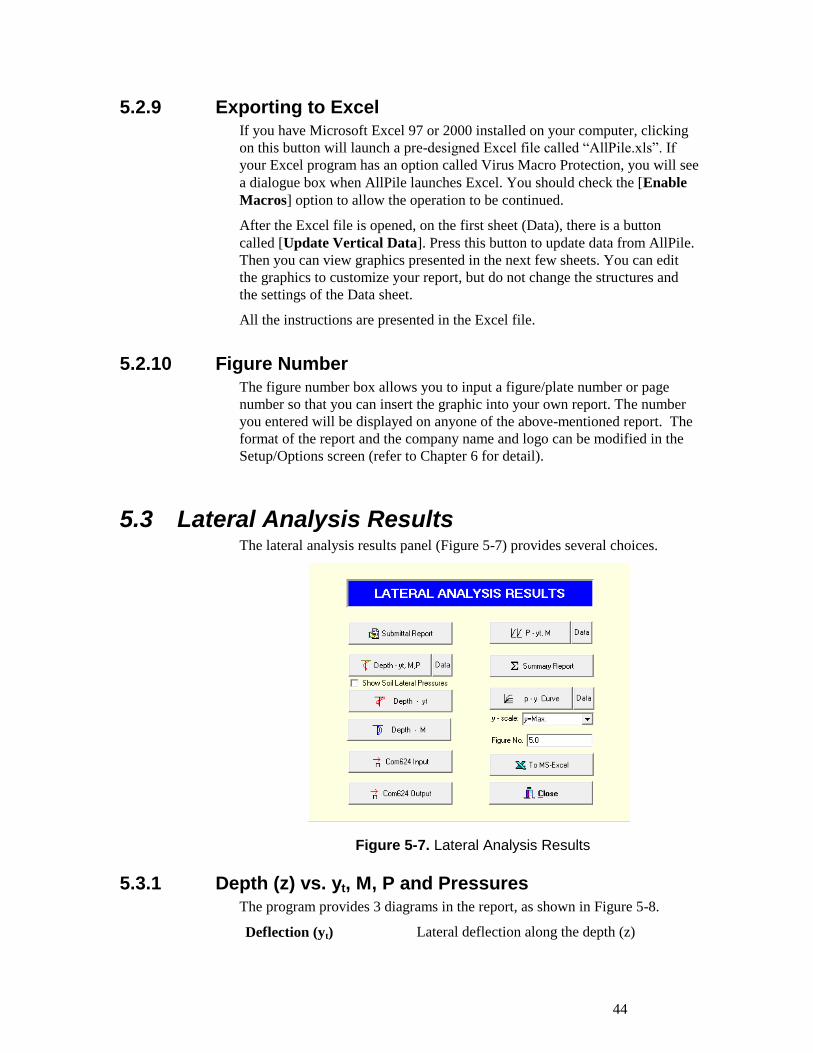
5.3 Lateral Analysis Results The lateral analysis results panel (Figure 5-7) provides several choices.
5.3.1 Depth (z) vs. yt, M, P and Pressures The program provides 3 diagrams in the report, as shown in Figure 5-8.
Deflection (yt) Lateral deflection along the depth (z)
Figure 5-7. Lateral Analysis Results
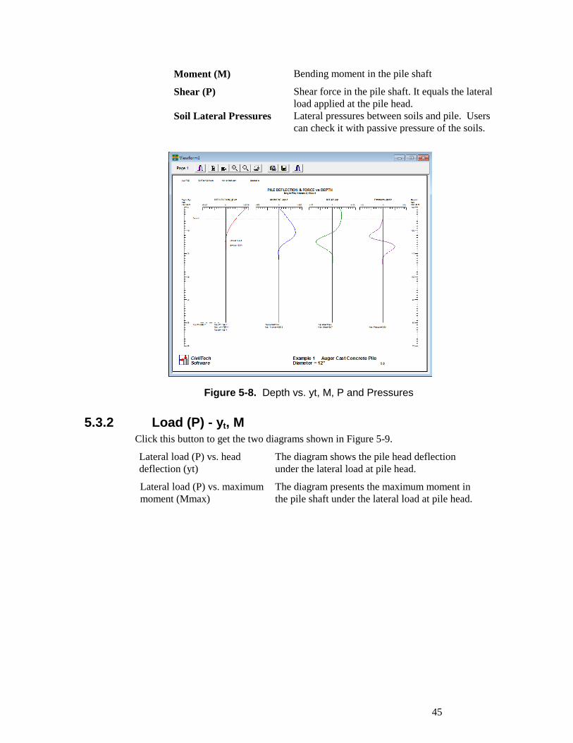
45
. . . . . . . . .
Moment (M) Bending moment in the pile shaft
Shear (P) Shear force in the pile shaft. It equals the lateral
load applied at the pile head.
Soil Lateral Pressures Lateral pressures between soils and pile. Users
can check it with passive pressure of the soils.
5.3.2 Load (P) - yt, M Click this button to get the two diagrams shown in Figure 5-9.
Lateral load (P) vs. head
deflection (yt)
The diagram shows the pile head deflection
under the lateral load at pile head.
Lateral load (P) vs. maximum
moment (Mmax)
The diagram presents the maximum moment in
the pile shaft under the lateral load at pile head.
Figure 5-8. Depth vs. yt, M, P and Pressures
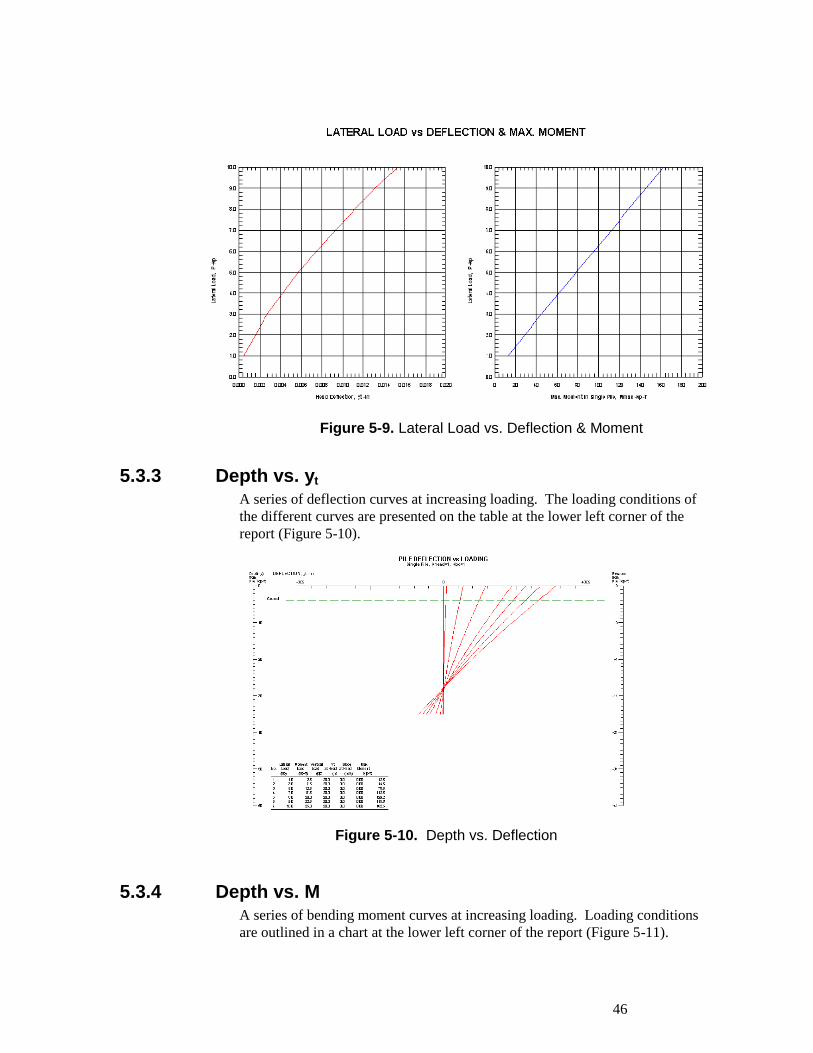
46
. . . . . . . . .
5.3.3 Depth vs. yt
A series of deflection curves at increasing loading. The loading conditions of
the different curves are presented on the table at the lower left corner of the
report (Figure 5-10).
5.3.4 Depth vs. M A series of bending moment curves at increasing loading. Loading conditions
are outlined in a chart at the lower left corner of the report (Figure 5-11).
Figure 5-9. Lateral Load vs. Deflection & Moment
Figure 5-10. Depth vs. Deflection
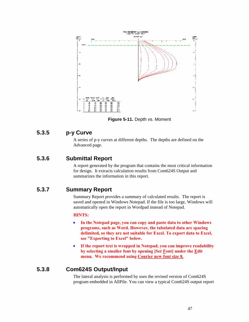
47
. . . . . . . . .
5.3.5 p-y Curve A series of p-y curves at different depths. The depths are defined on the
Advanced page.
5.3.6 Submittal Report A report generated by the program that contains the most critical information
for design. It extracts calculation results from Com624S Output and
summarizes the information in this report.
5.3.7 Summary Report Summary Report provides a summary of calculated results. The report is
saved and opened in Windows Notepad. If the file is too large, Windows will
automatically open the report in Wordpad instead of Notepad.
HINTS:
In the Notepad page, you can copy and paste data to other Windows
programs, such as Word. However, the tabulated data are spacing
delimited, so they are not suitable for Excel. To export data to Excel,
see "Exporting to Excel" below.
If the report text is wrapped in Notepad, you can improve readability
by selecting a smaller font by opening [Set Font] under the Edit
menu. We recommend using Courier new font size 8.
5.3.8 Com624S Output/Input The lateral analysis is performed by uses the revised version of Com624S
program embedded in AllPile. You can view a typical Com624S output report
Figure 5-11. Depth vs. Moment
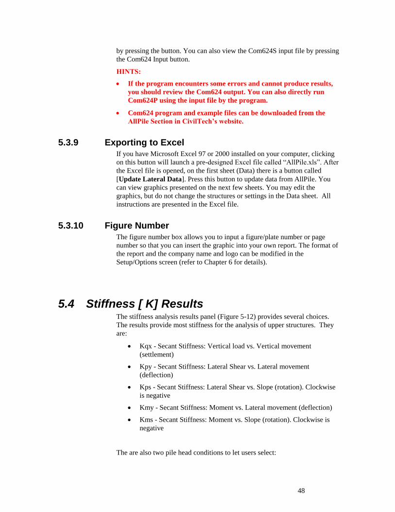
48
. . . . . . . . .
by pressing the button. You can also view the Com624S input file by pressing
the Com624 Input button.
HINTS:
If the program encounters some errors and cannot produce results,
you should review the Com624 output. You can also directly run
Com624P using the input file by the program.
Com624 program and example files can be downloaded from the
AllPile Section in CivilTech’s website.
5.3.9 Exporting to Excel If you have Microsoft Excel 97 or 2000 installed on your computer, clicking
on this button will launch a pre-designed Excel file called “AllPile.xls”. After
the Excel file is opened, on the first sheet (Data) there is a button called
[Update Lateral Data]. Press this button to update data from AllPile. You
can view graphics presented on the next few sheets. You may edit the
graphics, but do not change the structures or settings in the Data sheet. All
instructions are presented in the Excel file.
5.3.10 Figure Number The figure number box allows you to input a figure/plate number or page
number so that you can insert the graphic into your own report. The format of
the report and the company name and logo can be modified in the
Setup/Options screen (refer to Chapter 6 for details).
5.4 Stiffness [ K] Results The stiffness analysis results panel (Figure 5-12) provides several choices.
The results provide most stiffness for the analysis of upper structures. They
are:
Kqx - Secant Stiffness: Vertical load vs. Vertical movement
(settlement)
Kpy - Secant Stiffness: Lateral Shear vs. Lateral movement
(deflection)
Kps - Secant Stiffness: Lateral Shear vs. Slope (rotation). Clockwise
is negative
Kmy - Secant Stiffness: Moment vs. Lateral movement (deflection)
Kms - Secant Stiffness: Moment vs. Slope (rotation). Clockwise is
negative
The are also two pile head conditions to let users select:
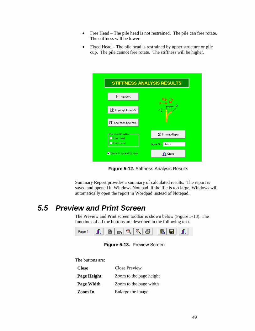
49
. . . . . . . . .
Free Head – The pile head is not restrained. The pile can free rotate.
The stiffness will be lower.
Fixed Head – The pile head is restrained by upper structure or pile
cup. The pile cannot free rotate. The stiffness will be higher.
Summary Report provides a summary of calculated results. The report is
saved and opened in Windows Notepad. If the file is too large, Windows will
automatically open the report in Wordpad instead of Notepad.
5.5 Preview and Print Screen The Preview and Print screen toolbar is shown below (Figure 5-13). The
functions of all the buttons are described in the following text.
The buttons are:
Close
Page Height
Close Preview
Zoom to the page height
Page Width Zoom to the page width
Zoom In Enlarge the image
Figure 5-13. Preview Screen
Figure 5-12. Stiffness Analysis Results
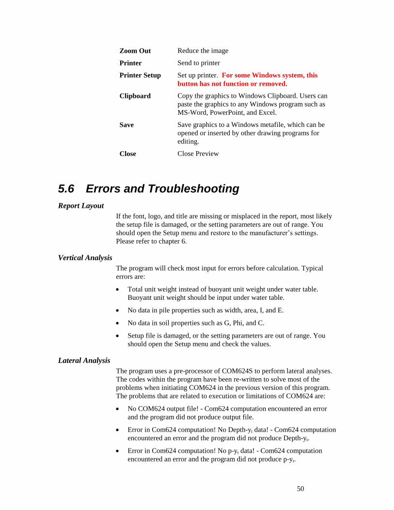
50
. . . . . . . . .
Zoom Out Reduce the image
Printer Send to printer
Printer Setup Set up printer. For some Windows system, this
button has not function or removed.
Clipboard Copy the graphics to Windows Clipboard. Users can
paste the graphics to any Windows program such as
MS-Word, PowerPoint, and Excel.
Save Save graphics to a Windows metafile, which can be
opened or inserted by other drawing programs for
editing.
Close Close Preview
5.6 Errors and Troubleshooting
Report Layout
If the font, logo, and title are missing or misplaced in the report, most likely
the setup file is damaged, or the setting parameters are out of range. You
should open the Setup menu and restore to the manufacturer’s settings.
Please refer to chapter 6.
Vertical Analysis
The program will check most input for errors before calculation. Typical
errors are:
Total unit weight instead of buoyant unit weight under water table.
Buoyant unit weight should be input under water table.
No data in pile properties such as width, area, I, and E.
No data in soil properties such as G, Phi, and C.
Setup file is damaged, or the setting parameters are out of range. You
should open the Setup menu and check the values.
Lateral Analysis
The program uses a pre-processor of COM624S to perform lateral analyses.
The codes within the program have been re-written to solve most of the
problems when initiating COM624 in the previous version of this program.
The problems that are related to execution or limitations of COM624 are:
No COM624 output file! - Com624 computation encountered an error
and the program did not produce output file.
Error in Com624 computation! No Depth-yt data! - Com624 computation
encountered an error and the program did not produce Depth-yt.
Error in Com624 computation! No p-yt data! - Com624 computation
encountered an error and the program did not produce p-yt.
51
. . . . . . . . .
If any one of the above warnings is encountered, please check the data. Most
of the cases are related to excessive calculated deflection, which exceeds the
allowable yt. This causes COM624 to terminate the calculations. The problem
occurs when the pile is too flexible, soils are too soft, or load is too large.
Pile too flexible – If the I and E of the pile section are too small,
COM624 stops.
Soils are too soft or loose – If Phi or K is too small for sandy soils and C
or e50 is too small for cohesive soils, COM624 stops.
Load is too large – If P, M, or yt is too large, COM624 stops.
Large surface slope angle or batter angle – If the surface or batter angle is
larger than the soil friction angle, COM624 stops.
Large H – If the distance between pile top and ground surface is too
large, COM624 stops.
HINT: view the COM624 OUTPUT report to get the error message.
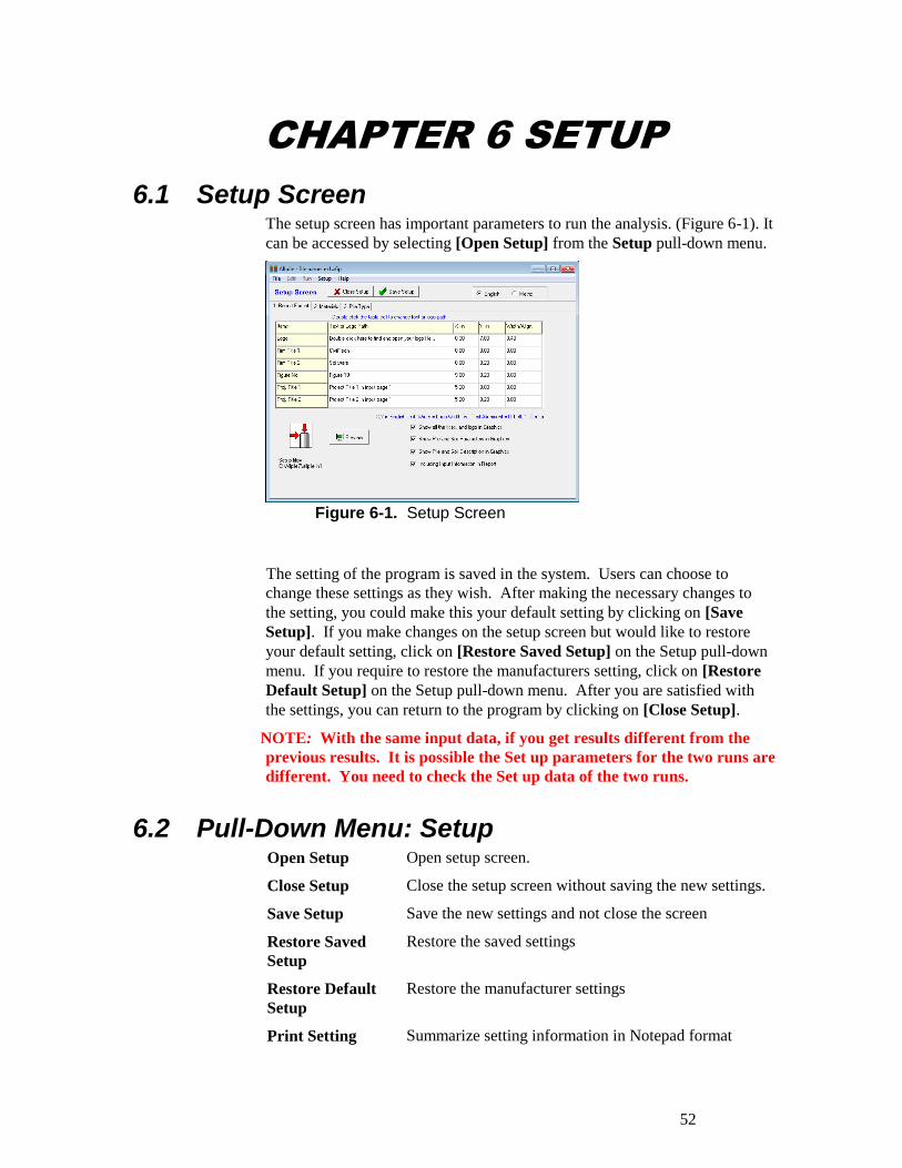
52
. . . . . . . . .
CHAPTER 6 SETUP
6.1 Setup Screen The setup screen has important parameters to run the analysis. (Figure 6-1). It
can be accessed by selecting [Open Setup] from the Setup pull-down menu.
The setting of the program is saved in the system. Users can choose to
change these settings as they wish. After making the necessary changes to
the setting, you could make this your default setting by clicking on [Save
Setup]. If you make changes on the setup screen but would like to restore
your default setting, click on [Restore Saved Setup] on the Setup pull-down
menu. If you require to restore the manufacturers setting, click on [Restore
Default Setup] on the Setup pull-down menu. After you are satisfied with
the settings, you can return to the program by clicking on [Close Setup].
NOTE: With the same input data, if you get results different from the
previous results. It is possible the Set up parameters for the two runs are
different. You need to check the Set up data of the two runs.
6.2 Pull-Down Menu: Setup Open Setup Open setup screen.
Close Setup Close the setup screen without saving the new settings.
Save Setup Save the new settings and not close the screen
Restore Saved
Setup
Restore the saved settings
Restore Default
Setup
Restore the manufacturer settings
Print Setting Summarize setting information in Notepad format
Figure 6-1. Setup Screen
53
. . . . . . . . .
which allows you to print
6.3 Speed Bar The speed bar has two buttons:
Save Setup Save the modified settings
Close Setup Close the setup screen and return to the program
6.4 Tabbed Pages The three tabbed pages are summarized below. Each page is described in
detail in this chapter.
1. Report Format Customize graphical output (reports)
2. Materials Configure pile materials
3. Pile Type Configure pile type and method code
6.4.1 1. Report Format Page You can customize the format of the output report by designating the position
of each item. The location of each item are position based on coordinates,
where (0,0) is located at the upper left corner of the page. Positive X is in the
direction to the right, and positive Y is in the direction vertically downwards.
The units of measurements are in inches or centimeters.
The items listed in the rows are as follows:
Logo The logo shown in the report can be a bmp, gif, or jpeg
file. Double click the row to specify the file path. The
width of the logo can be changed on the right most
column (W) in inches or centimeters.
Firm Title 1 Your company name is presented here. X and Y define
the coordinates. Double click the row to select text font.
Firm Title 2 You may enter a company subtitle here. X and Y define
the coordinates. Double click the row to select text font.
Figure Number The page or figure number in the report. X and Y define
the coordinates. Double click the row to select text font.
The page number shown in the table is a dummy. The
actual text in the report is from the Lateral Analysis
Result or Vertical Analysis Result panel.
Project Title 1
& Project Title 2
This row specifies the location and font of the project
title. X and Y define the coordinates. The text shown in
the table is a dummy. The actual text in the report is
from the Pile Type page.
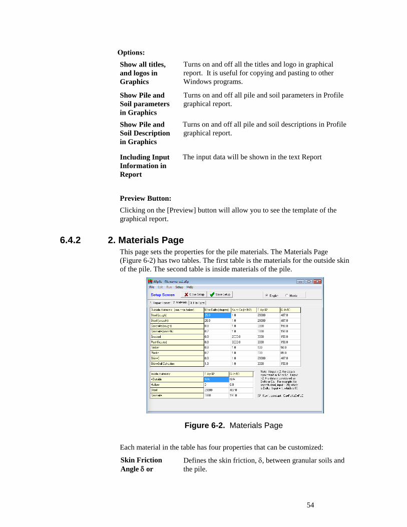
54
. . . . . . . . .
Options:
Show all titles,
and logos in
Graphics
Turns on and off all the titles and logo in graphical
report. It is useful for copying and pasting to other
Windows programs.
Show Pile and
Soil parameters
in Graphics
Turns on and off all pile and soil parameters in Profile
graphical report.
Show Pile and
Soil Description
in Graphics
Turns on and off all pile and soil descriptions in Profile
graphical report.
Including Input
Information in
Report
The input data will be shown in the text Report
Preview Button:
Clicking on the [Preview] button will allow you to see the template of the
graphical report.
6.4.2 2. Materials Page This page sets the properties for the pile materials. The Materials Page
(Figure 6-2) has two tables. The first table is the materials for the outside skin
of the pile. The second table is inside materials of the pile.
Each material in the table has four properties that can be customized:
Skin Friction
Angle or
Defines the skin friction, , between granular soils and
the pile.
Figure 6-2. Materials Page
55
. . . . . . . . .
Faction Kf
If you input a value > 2, the program will recognize
it as skin friction ()
If you input a value ranging from 0.1 to 2, the
program recognizes it as Kf . The program
multiplies Kf by the soil internal friction, to get
the skin friction, :
= Kf
Where, Kf – friction factor (0.1 ~ 2)
NOTE: Internal friction, , is the friction between
granular soil particles. Skin friction, , is the skin
friction between soil and pile. is not the same as -
- usually is less than .
Adhesion Ca or
Factor Kc
Defines the adhesion, Ca, between cohesive soils and
the pile.
If you input a value >2, the program recognizes it as
adhesion, Ca.
If you input a factor (range 0.1 to 2), the program
recognizes it as Kc. The program multiplies Kc by the
soil cohesion, C, to get the adhesion, Ca:
Ca = Kc KaC
Where,
Ka – adhesion factor (0.1 ~ 2). Users define it.
Ka – adhesion ratio (0.1 ~ 1.5). Program defines it
based on pile type and C (See Chapter 8).
Ka can be set to 1. It will bypass Ka calculation. This
option is in a check box of this page.
NOTE: Cohesion, C, is the shear strength between
cohesive soils. Adhesion, Ca, is the shear resistance
between soil and pile. Ca is not equal to C. Usually
Ca is less than C.
E Defines elastic modulus of pile materials.
G Specifies unit weight of pile materials.
The second table is the materials properties of the inside of the pile. For
example, a steel pipe pile filled with concrete has outside materials = steel
and inside materials = concrete. A concrete pile with steel bars has outside
materials = concrete and inside materials = steel. The material properties can
be customized:
E Defines elastic modulus of inside pile materials.
G Specifies unit weight of inside pile materials.
Check Box for Ka=1: See explanation of Ca and Kc above.
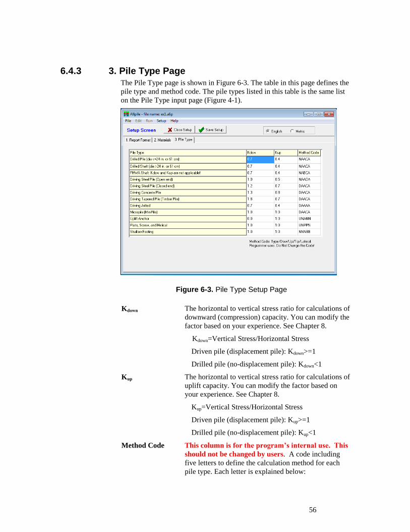
56
. . . . . . . . .
6.4.3 3. Pile Type Page The Pile Type page is shown in Figure 6-3. The table in this page defines the
pile type and method code. The pile types listed in this table is the same list
on the Pile Type input page (Figure 4-1).
Kdown The horizontal to vertical stress ratio for calculations of
downward (compression) capacity. You can modify the
factor based on your experience. See Chapter 8.
Kdown=Vertical Stress/Horizontal Stress
Driven pile (displacement pile): Kdown>=1
Drilled pile (no-displacement pile): Kdown<1
Kup The horizontal to vertical stress ratio for calculations of
uplift capacity. You can modify the factor based on
your experience. See Chapter 8.
Kup=Vertical Stress/Horizontal Stress
Driven pile (displacement pile): Kup>=1
Drilled pile (no-displacement pile): Kup<1
Method Code This column is for the program’s internal use. This
should not be changed by users. A code including
five letters to define the calculation method for each
pile type. Each letter is explained below:
Figure 6-3. Pile Type Setup Page
Figure 6-2. Pile Type Page
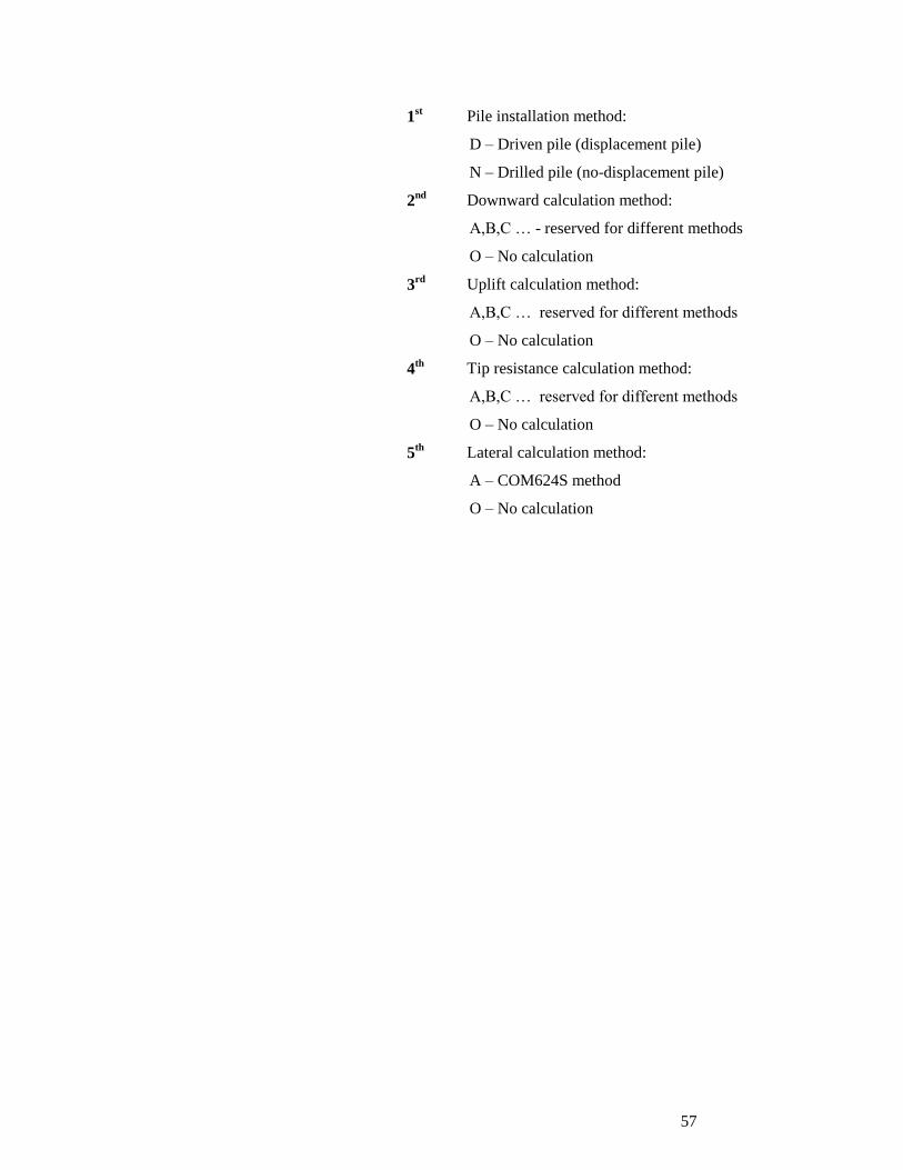
57
. . . . . . . . .
1st Pile installation method:
D – Driven pile (displacement pile)
N – Drilled pile (no-displacement pile)
2nd
Downward calculation method:
A,B,C … - reserved for different methods
O – No calculation
3rd
Uplift calculation method:
A,B,C … reserved for different methods
O – No calculation
4th
Tip resistance calculation method:
A,B,C … reserved for different methods
O – No calculation
5th
Lateral calculation method:
A – COM624S method
O – No calculation
58
. . . . . . . . .
CHAPTER 7 SAMPLES
7.1 Samples Samples with different soil conditions and pile types are included in the program. These
examples are intended to demonstrate the capabilities of the program and allow users to
learn more about the input process and other key functions. The samples include:
1. Auger Cast Concrete Pile
2. Drilled Shaft No Bell
3. Drilled Shaft with Bell
4. FHWA SHAFT Method with Bell
5. Driving Steel Pipe, Close Ended
6. Driving Steel Pipe, Open Ended
7. Driving Steel H Pile, Open Ended
8. Driving Steel Pile in Sloped Ground
9. Driving Steel Pile with Battered Angle
10. Driving Concrete Pile with Battered Angle
11. Driving Concrete Pile with Stinger
12. Driving Timber Pile with Battered Angle
13. Driving Jetted Pile
14. Micropile with Pressure Grout
15. Uplift Anchor based on Soil Strength
16. Uplift Anchor based on Bound Strength
17. Uplift Plate in Shallow Mode
18. Uplift Plate in Deep Mode
19. Shallow Foundation
20. COM624 Sample 1, One Soil
21. COM624 Sample 2, Five Soils
22. COM624 Sample 3, in Butter Angle
23. COM624 Sample 4, P-Y Input
24. COM624 Sample 5, Sloped Ground
25. Group Steel Piles
26. Group Auger Cast Piles
27. Group Pre-cast Concrete Piles
28. Tower Mono-Pile
29. Tower with 3 Piles
30. Tower with 4 Piles
Please open the sample files stored in the program and run them to see the input and
output data. The samples are in English units. For Metric (SI) units, open the sample
then choose metric on the Pile Type page.
59
. . . . . . . . .
CHAPTER 8
CALCULATION THEORY
.
CHAPTER 8 CALCULATION THEORY
Detailed in this chapter:
The theories behind the
program
The equations and methods
that are use to perform the
analyses.
Volume 2
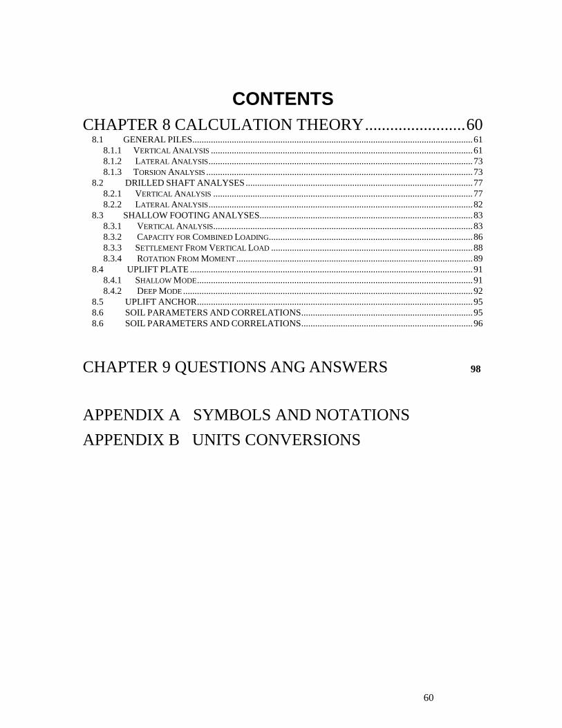
60
. . . . . . . . .
CONTENTS
CHAPTER 8 CALCULATION THEORY ........................ 60
8.1 GENERAL PILES ......................................................................................................................... 61 8.1.1 VERTICAL ANALYSIS ................................................................................................................. 61 8.1.2 LATERAL ANALYSIS .................................................................................................................. 73
8.1.3 TORSION ANALYSIS ................................................................................................................... 73
8.2 DRILLED SHAFT ANALYSES .................................................................................................. 77 8.2.1 VERTICAL ANALYSIS ................................................................................................................ 77 8.2.2 LATERAL ANALYSIS .................................................................................................................. 82
8.3 SHALLOW FOOTING ANALYSES............................................................................................ 83 8.3.1 VERTICAL ANALYSIS ................................................................................................................ 83 8.3.2 CAPACITY FOR COMBINED LOADING ........................................................................................ 86 8.3.3 SETTLEMENT FROM VERTICAL LOAD ....................................................................................... 88 8.3.4 ROTATION FROM MOMENT ...................................................................................................... 89
8.4 UPLIFT PLATE .......................................................................................................................... 91 8.4.1 SHALLOW MODE ....................................................................................................................... 91 8.4.2 DEEP MODE ............................................................................................................................. 92
8.5 UPLIFT ANCHOR ....................................................................................................................... 95 8.6 SOIL PARAMETERS AND CORRELATIONS .......................................................................... 95 8.6 SOIL PARAMETERS AND CORRELATIONS .......................................................................... 96
CHAPTER 9 QUESTIONS ANG ANSWERS 98
APPENDIX A SYMBOLS AND NOTATIONS
APPENDIX B UNITS CONVERSIONS
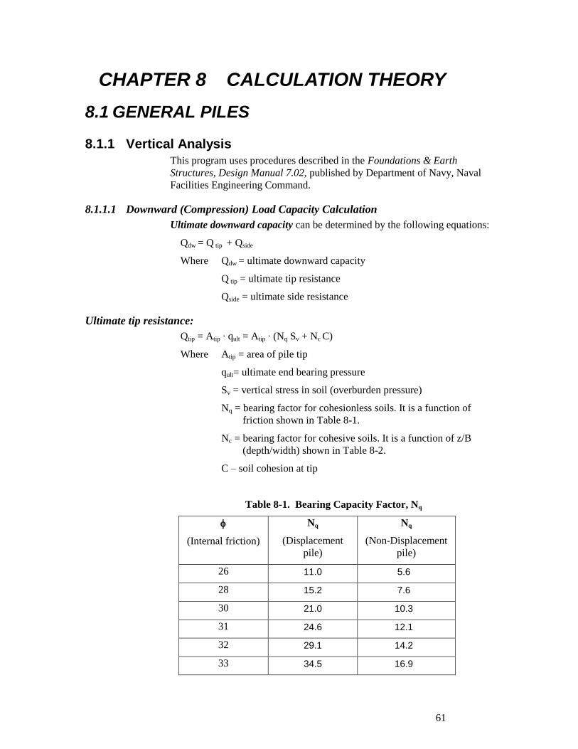
61
. . . . . . . . .
CHAPTER 8 CALCULATION THEORY
8.1 GENERAL PILES
8.1.1 Vertical Analysis This program uses procedures described in the Foundations & Earth
Structures, Design Manual 7.02, published by Department of Navy, Naval
Facilities Engineering Command.
8.1.1.1 Downward (Compression) Load Capacity Calculation
Ultimate downward capacity can be determined by the following equations:
Qdw = Q tip + Qside
Where Qdw = ultimate downward capacity
Q tip = ultimate tip resistance
Qside = ultimate side resistance
Ultimate tip resistance:
Qtip = Atip ∙ qult = Atip ∙ (Nq Sv + Nc C)
Where Atip = area of pile tip
qult= ultimate end bearing pressure
Sv = vertical stress in soil (overburden pressure)
Nq = bearing factor for cohesionless soils. It is a function of
friction shown in Table 8-1.
Nc = bearing factor for cohesive soils. It is a function of z/B
(depth/width) shown in Table 8-2.
C – soil cohesion at tip
Table 8-1. Bearing Capacity Factor, Nq
(Internal friction)
Nq
(Displacement
pile)
Nq
(Non-Displacement
pile)
26 11.0 5.6
28 15.2 7.6
30 21.0 10.3
31 24.6 12.1
32 29.1 14.2
33 34.5 16.9
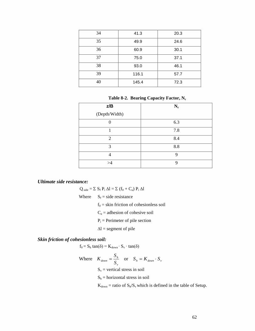
62
. . . . . . . . .
34 41.3 20.3
35 49.9 24.6
36 60.9 30.1
37 75.0 37.1
38 93.0 46.1
39 116.1 57.7
40 145.4 72.3
Table 8-2. Bearing Capacity Factor, Nc
z/B
(Depth/Width)
Nc
0 6.3
1 7.8
2 8.4
3 8.8
4 9
>4 9
Ultimate side resistance:
Q side = Sf Pi l = (f0 + Ca) Pi l
Where Sf = side resistance
f0 = skin friction of cohesionless soil
Ca = adhesion of cohesive soil
Pi = Perimeter of pile section
l = segment of pile
Skin friction of cohesionless soil:
f0 = Sh tan(δ) = Kdown ∙ Sv ∙ tan(δ)
Sv = vertical stress in soil
Sh = horizontal stress in soil
Kdown = ratio of Sh/Sv which is defined in the table of Setup.
vdownh
v
h
down SKSS
SK orWhere
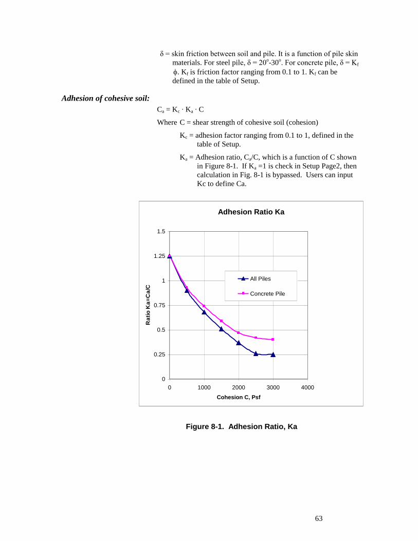
63
. . . . . . . . .
δ = skin friction between soil and pile. It is a function of pile skin
materials. For steel pile, δ = 20o-30
o. For concrete pile, δ = Kf
. Kf is friction factor ranging from 0.1 to 1. Kf can be
defined in the table of Setup.
Adhesion of cohesive soil:
Ca = Kc ∙ Ka ∙ C
Where C = shear strength of cohesive soil (cohesion)
Kc = adhesion factor ranging from 0.1 to 1, defined in the
table of Setup.
Ka = Adhesion ratio, Ca/C, which is a function of C shown
in Figure 8-1. If Ka =1 is check in Setup Page2, then
calculation in Fig. 8-1 is bypassed. Users can input
Kc to define Ca.
Adhesion Ratio Ka
0
0.25
0.5
0.75
1
1.25
1.5
0 1000 2000 3000 4000
Cohesion C, Psf
Ra
tio
Ka
=C
a/C
All Piles
Concrete Pile
Figure 8-1. Adhesion Ratio, Ka
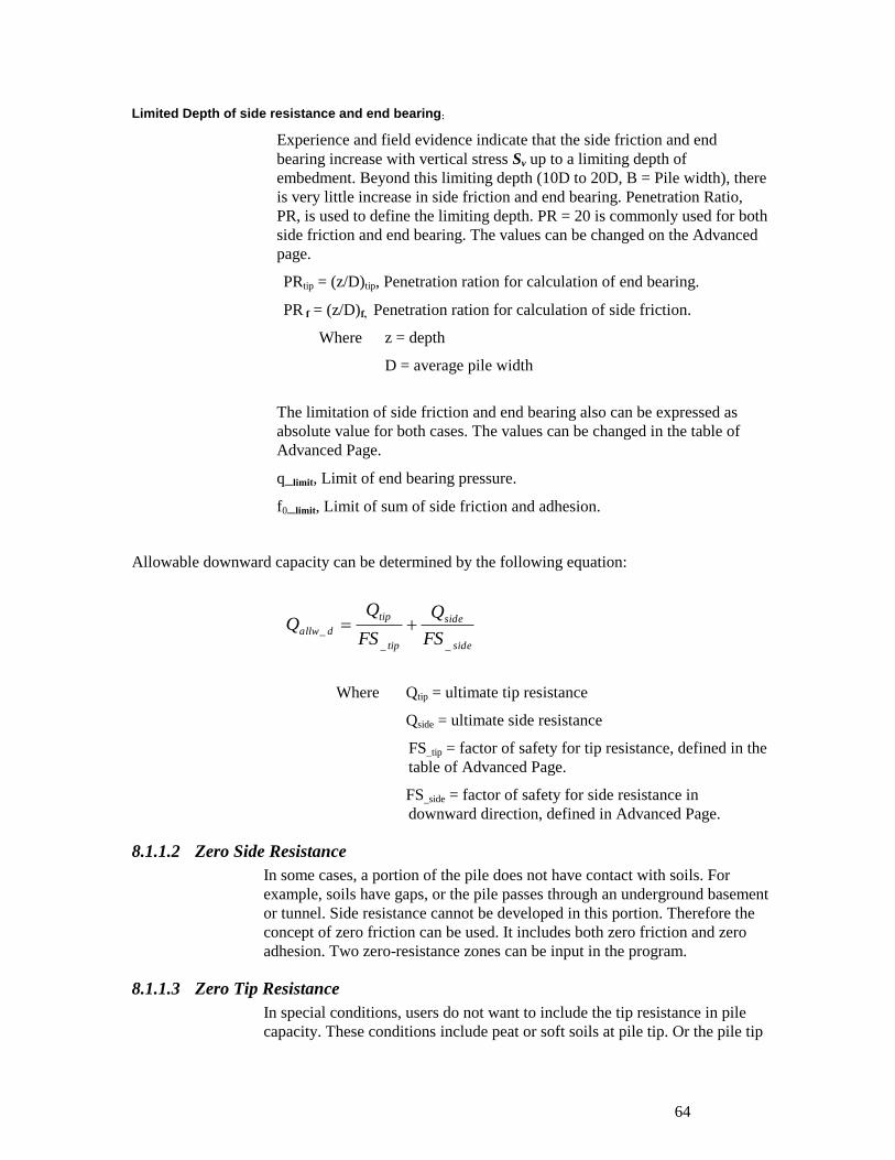
64
. . . . . . . . .
Limited Depth of side resistance and end bearing:
Experience and field evidence indicate that the side friction and end
bearing increase with vertical stress Sv up to a limiting depth of
embedment. Beyond this limiting depth (10D to 20D, B = Pile width), there
is very little increase in side friction and end bearing. Penetration Ratio,
PR, is used to define the limiting depth. PR = 20 is commonly used for both
side friction and end bearing. The values can be changed on the Advanced
page.
PRtip = (z/D)tip, Penetration ration for calculation of end bearing.
PR f = (z/D)f, Penetration ration for calculation of side friction.
Where z = depth
D = average pile width
The limitation of side friction and end bearing also can be expressed as
absolute value for both cases. The values can be changed in the table of
Advanced Page.
q_limit, Limit of end bearing pressure.
f0_limit, Limit of sum of side friction and adhesion.
Allowable downward capacity can be determined by the following equation:
Where Qtip = ultimate tip resistance
Qside = ultimate side resistance
FS_tip = factor of safety for tip resistance, defined in the
table of Advanced Page.
FS_side = factor of safety for side resistance in
downward direction, defined in Advanced Page.
8.1.1.2 Zero Side Resistance
In some cases, a portion of the pile does not have contact with soils. For
example, soils have gaps, or the pile passes through an underground basement
or tunnel. Side resistance cannot be developed in this portion. Therefore the
concept of zero friction can be used. It includes both zero friction and zero
adhesion. Two zero-resistance zones can be input in the program.
8.1.1.3 Zero Tip Resistance
In special conditions, users do not want to include the tip resistance in pile
capacity. These conditions include peat or soft soils at pile tip. Or the pile tip
side
side
tip
tip
dallwFS
Q
FS
__
_
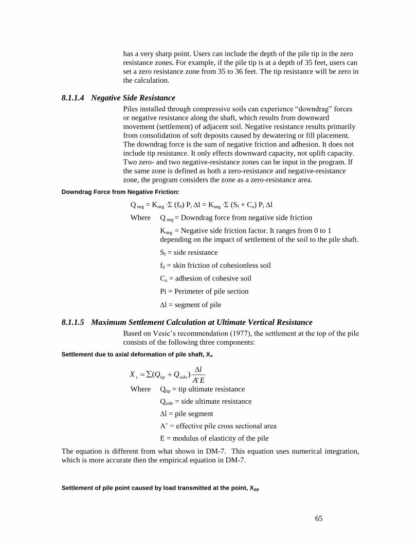
65
. . . . . . . . .
has a very sharp point. Users can include the depth of the pile tip in the zero
resistance zones. For example, if the pile tip is at a depth of 35 feet, users can
set a zero resistance zone from 35 to 36 feet. The tip resistance will be zero in
the calculation.
8.1.1.4 Negative Side Resistance
Piles installed through compressive soils can experience “downdrag” forces
or negative resistance along the shaft, which results from downward
movement (settlement) of adjacent soil. Negative resistance results primarily
from consolidation of soft deposits caused by dewatering or fill placement.
The downdrag force is the sum of negative friction and adhesion. It does not
include tip resistance. It only effects downward capacity, not uplift capacity.
Two zero- and two negative-resistance zones can be input in the program. If
the same zone is defined as both a zero-resistance and negative-resistance
zone, the program considers the zone as a zero-resistance area.
Downdrag Force from Negative Friction:
Q neg = Kneg ∙ (f0) Pi l = Kneg ∙ (Sf + Ca) Pi l
Where Q neg = Downdrag force from negative side friction
Kneg = Negative side friction factor. It ranges from 0 to 1
depending on the impact of settlement of the soil to the pile shaft.
Sf = side resistance
f0 = skin friction of cohesionless soil
Ca = adhesion of cohesive soil
Pi = Perimeter of pile section
l = segment of pile
8.1.1.5 Maximum Settlement Calculation at Ultimate Vertical Resistance
Based on Vesic’s recommendation (1977), the settlement at the top of the pile
consists of the following three components:
Settlement due to axial deformation of pile shaft, Xs
Where Qtip = tip ultimate resistance
Qside = side ultimate resistance
∆l = pile segment
A’ = effective pile cross sectional area
E = modulus of elasticity of the pile
The equation is different from what shown in DM-7. This equation uses numerical integration,
which is more accurate then the empirical equation in DM-7.
Settlement of pile point caused by load transmitted at the point, Xpp
EA
lQQX sidetips
')(
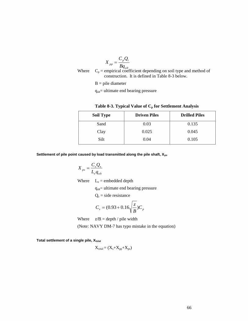
66
. . . . . . . . .
ult
tp
ppBq
QCX
Where Cp = empirical coefficient depending on soil type and method of
construction. It is defined in Table 8-3 below.
B = pile diameter
qult= ultimate end bearing pressure
Table 8-3. Typical Value of Cp for Settlement Analysis
Soil Type Driven Piles Drilled Piles
Sand 0.03 0.135
Clay 0.025 0.045
Silt 0.04 0.105
Settlement of pile point caused by load transmitted along the pile shaft, Xps
Where Le = embedded depth
qult= ultimate end bearing pressure
Qs = side resistance
ps CB
zC )16.093.0(
Where z/B = depth / pile width
(Note: NAVY DM-7 has typo mistake in the equation)
Total settlement of a single pile, Xtotal
Xtotal = (Xs+Xpp+Xps)
ulte
ss
psqL
QCX
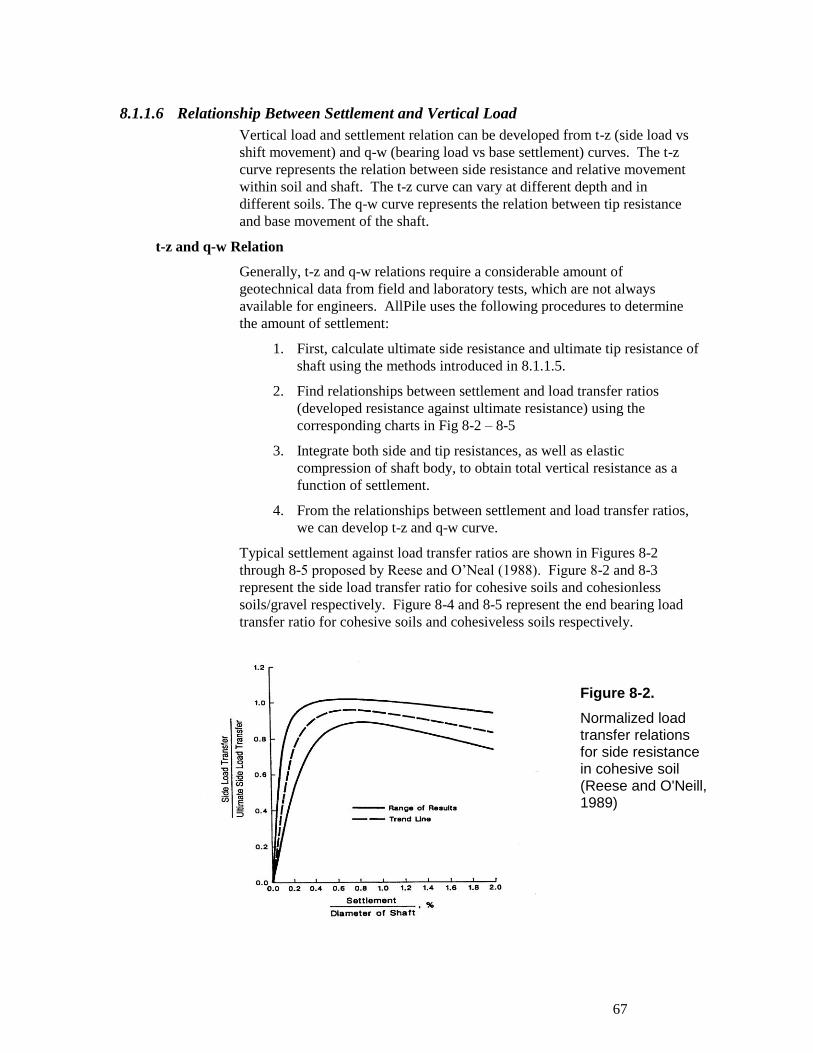
67
. . . . . . . . .
8.1.1.6 Relationship Between Settlement and Vertical Load
Vertical load and settlement relation can be developed from t-z (side load vs
shift movement) and q-w (bearing load vs base settlement) curves. The t-z
curve represents the relation between side resistance and relative movement
within soil and shaft. The t-z curve can vary at different depth and in
different soils. The q-w curve represents the relation between tip resistance
and base movement of the shaft.
t-z and q-w Relation
Generally, t-z and q-w relations require a considerable amount of
geotechnical data from field and laboratory tests, which are not always
available for engineers. AllPile uses the following procedures to determine
the amount of settlement:
1. First, calculate ultimate side resistance and ultimate tip resistance of
shaft using the methods introduced in 8.1.1.5.
2. Find relationships between settlement and load transfer ratios
(developed resistance against ultimate resistance) using the
corresponding charts in Fig 8-2 – 8-5
3. Integrate both side and tip resistances, as well as elastic
compression of shaft body, to obtain total vertical resistance as a
function of settlement.
4. From the relationships between settlement and load transfer ratios,
we can develop t-z and q-w curve.
Typical settlement against load transfer ratios are shown in Figures 8-2
through 8-5 proposed by Reese and O’Neal (1988). Figure 8-2 and 8-3
represent the side load transfer ratio for cohesive soils and cohesionless
soils/gravel respectively. Figure 8-4 and 8-5 represent the end bearing load
transfer ratio for cohesive soils and cohesiveless soils respectively.
Figure 8-2.
Normalized load transfer relations for side resistance in cohesive soil (Reese and O'Neill, 1989)
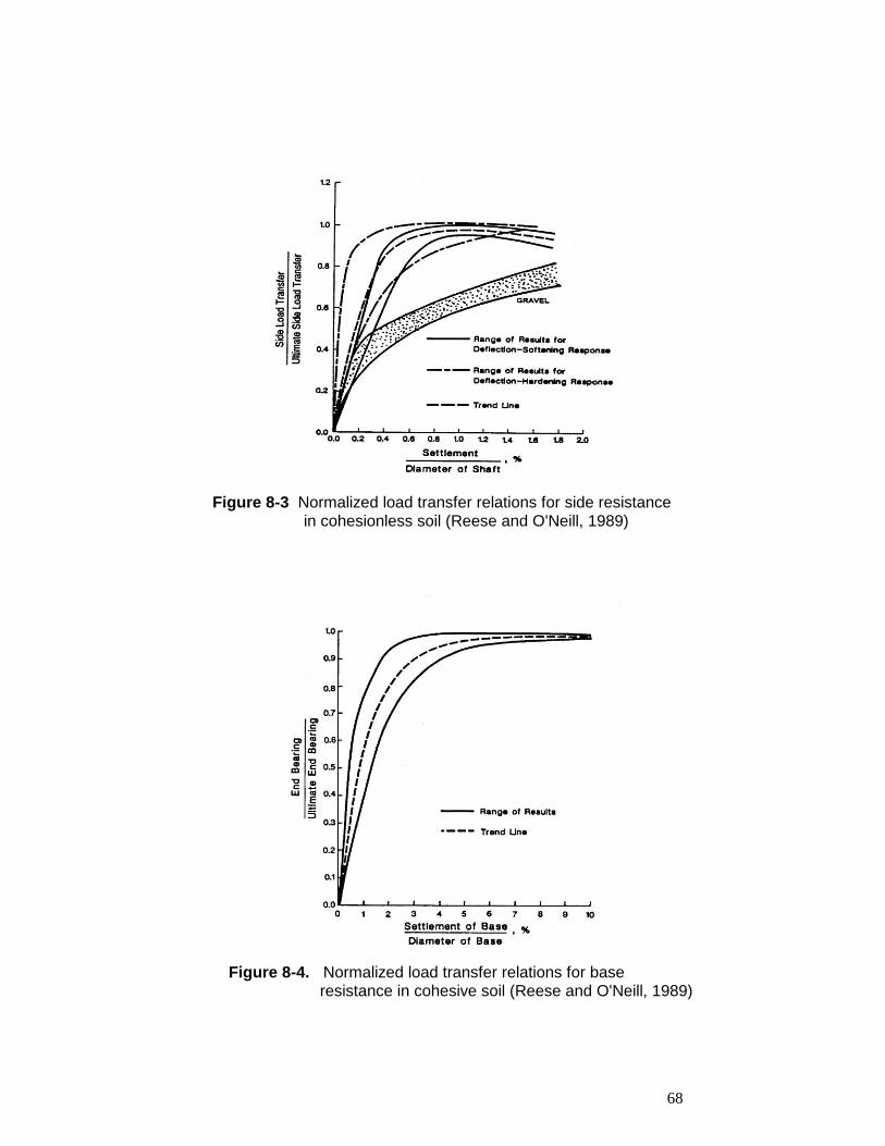
68
. . . . . . . . .
Figure 8-3 Normalized load transfer relations for side resistance in cohesionless soil (Reese and O'Neill, 1989)
Figure 8-4. Normalized load transfer relations for base resistance in cohesive soil (Reese and O'Neill, 1989)
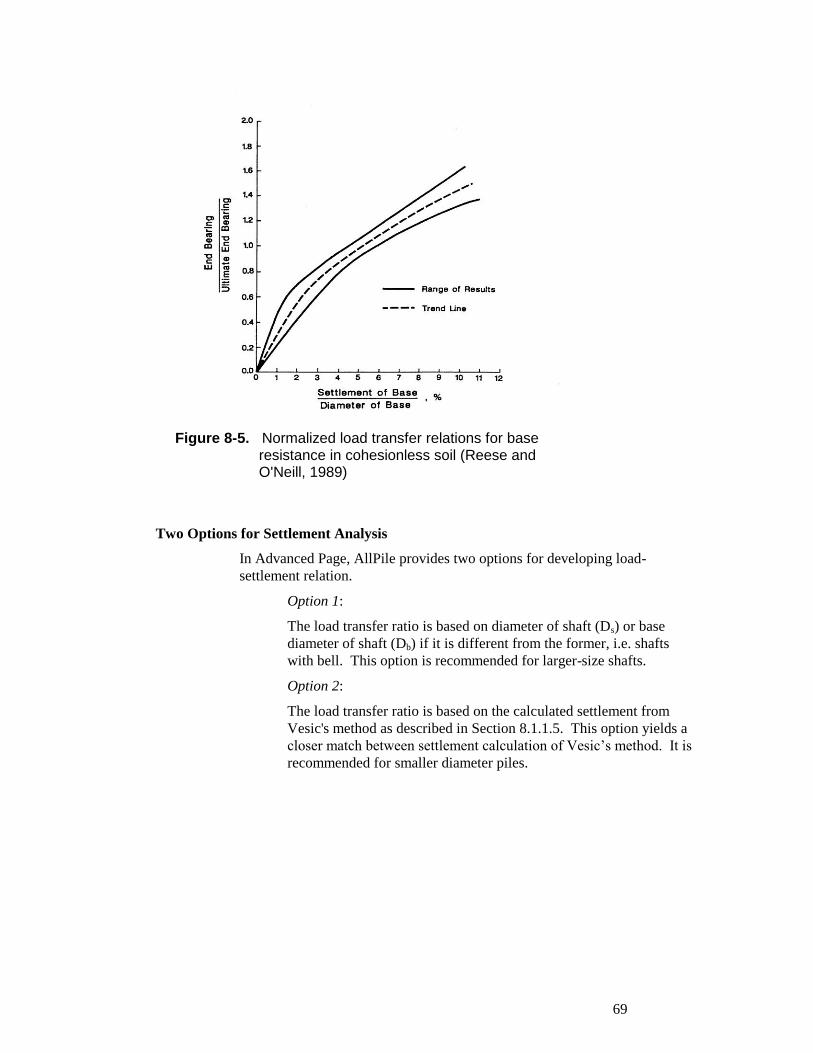
69
. . . . . . . . .
Two Options for Settlement Analysis
In Advanced Page, AllPile provides two options for developing load-
settlement relation.
Option 1:
The load transfer ratio is based on diameter of shaft (Ds) or base
diameter of shaft (Db) if it is different from the former, i.e. shafts
with bell. This option is recommended for larger-size shafts.
Option 2:
The load transfer ratio is based on the calculated settlement from
Vesic's method as described in Section 8.1.1.5. This option yields a
closer match between settlement calculation of Vesic’s method. It is
recommended for smaller diameter piles.
Figure 8-5. Normalized load transfer relations for base resistance in cohesionless soil (Reese and O'Neill, 1989)
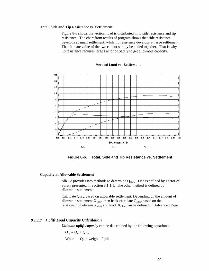
70
. . . . . . . . .
Total, Side and Tip Resistance vs. Settlement
Figure 8-6 shows the vertical load is distributed in to side resistance and tip
resistance. The chart from results of program shows that side resistance
develops at small settlement, while tip resistance develops at large settlement.
The ultimate value of the two cannot simply be added together. That is why
tip resistance requires large Factor of Safety to get allowable capacity.
Capacity at Allowable Settlement
AllPile provides two methods to determine Qallow. One is defined by Factor of
Safety presented in Section 8.1.1.1. The other method is defined by
allowable settlement.
Calculate Qallow based on allowable settlement. Depending on the amount of
allowable settlement Xallow, then back-calculate Qallow based on the
relationship between Xallow and load. Xallow can be defined on Advanced Page.
8.1.1.7 Uplift Load Capacity Calculation
Ultimate uplift capacity can be determined by the following equations:
Qup = Qw + Qside
Where Qw = weight of pile
Figure 8-6. Total, Side and Tip Resistance vs. Settlement
71
. . . . . . . . .
Qside = ultimate side resistance
Qw = ∑Wi ∆l
Where Wi = weight of pile section in unit length
∆l = segment of pile
Q side = Sf Pi∙l = (f0 + Ca) Pi l
Where Sf = side resistance
f0 = skin friction of cohesionless soil
Ca = adhesion of cohesive soil
l = segment of pile
Pi = Perimeter of pile section
f0 = Kup ∙Sv tanδ
Sv = vertical stress in soil
Sh = horizontal stress in soil
Kup = ratio of Sh/Sv which is defined in the table of Setup
δ = skin friction between soil and pile. It is function of pile side
materials. For steel pile, δ = 20o-30
o. For concrete pile, δ = KfФ.
Kf is a friction factor ranging from 0.1 to 1. Kf can be defined in in
the table of Setup.
Ca = Kc ∙ Ka ∙ C
Where C = shear strength of cohesive soil (cohesion)
Kc = adhesion factor ranging from 0.1 to 1, defined in the table of
Setup.
Ka = Adhesion ratio, Ca/C, which is a function of C shown in
Figure 8-1.
Allowable Uplift Capacity can be determined by following equations:
Where Qw = weight of pile
vuph
v
h
up SKSorS
SK Where
up
side
w
wUallw
FS
Q
FS
__
_
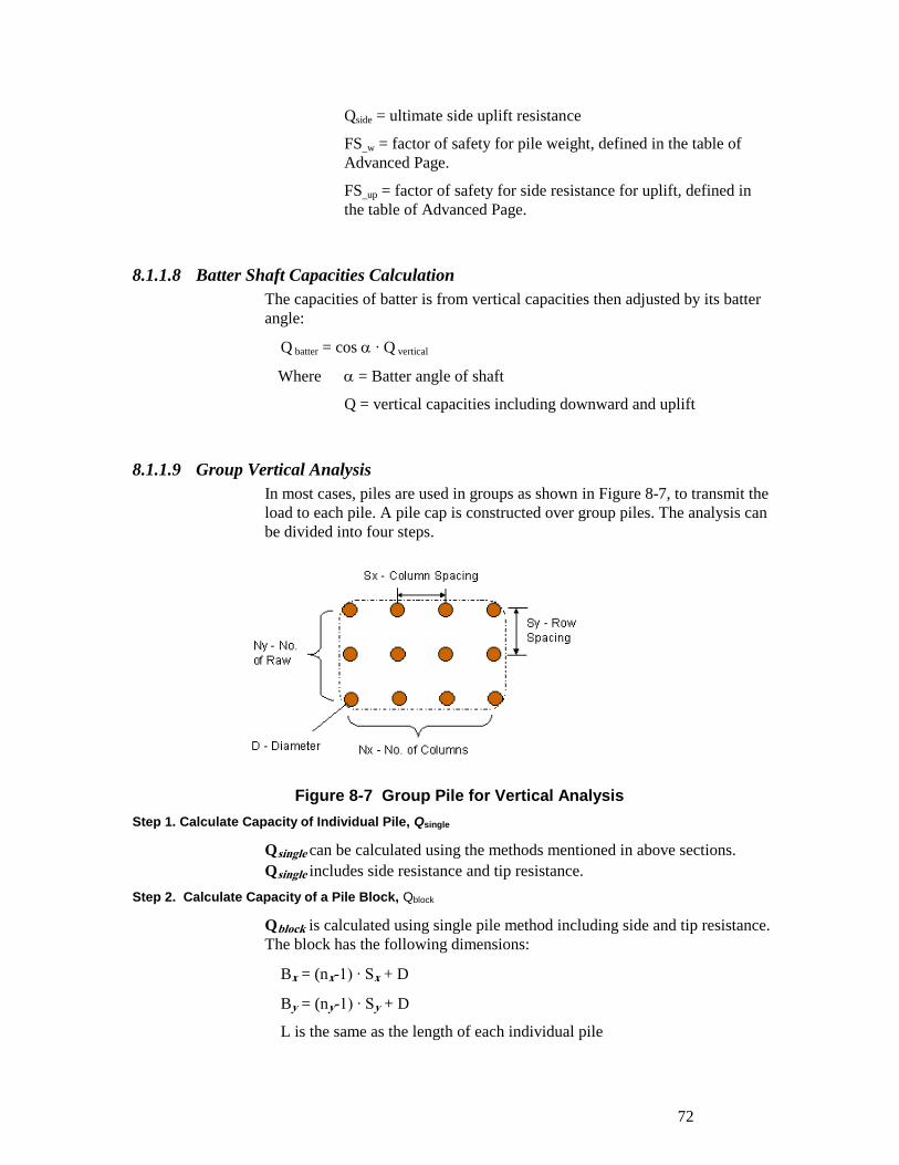
72
. . . . . . . . .
Qside = ultimate side uplift resistance
FS_w = factor of safety for pile weight, defined in the table of
Advanced Page.
FS_up = factor of safety for side resistance for uplift, defined in
the table of Advanced Page.
8.1.1.8 Batter Shaft Capacities Calculation
The capacities of batter is from vertical capacities then adjusted by its batter
angle:
Q batter = cos ∙ Q vertical
Where = Batter angle of shaft
Q = vertical capacities including downward and uplift
8.1.1.9 Group Vertical Analysis
In most cases, piles are used in groups as shown in Figure 8-7, to transmit the
load to each pile. A pile cap is constructed over group piles. The analysis can
be divided into four steps.
Figure 8-7 Group Pile for Vertical Analysis
Step 1. Calculate Capacity of Individual Pile, Qsingle
Qsingle can be calculated using the methods mentioned in above sections.
Qsingle includes side resistance and tip resistance.
Step 2. Calculate Capacity of a Pile Block, Qblock
Qblock is calculated using single pile method including side and tip resistance.
The block has the following dimensions:
Bx = (nx-1) ∙ Sx + D
By = (ny-1) ∙ Sy + D
L is the same as the length of each individual pile
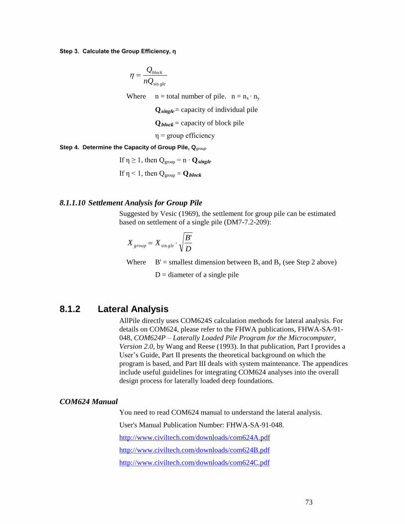
73
. . . . . . . . .
Step 3. Calculate the Group Efficiency, η
Where n = total number of pile. n = nx ∙ ny
Qsingle = capacity of individual pile
Qblock = capacity of block pile
η = group efficiency
Step 4. Determine the Capacity of Group Pile, Qgroup
If η ≥ 1, then Qgroup = n ∙ Qsingle
If η < 1, then Qgroup = Qblock
8.1.1.10 Settlement Analysis for Group Pile
Suggested by Vesic (1969), the settlement for group pile can be estimated
based on settlement of a single pile (DM7-7.2-209):
Where B' = smallest dimension between Bx and By (see Step 2 above)
D = diameter of a single pile
8.1.2 Lateral Analysis AllPile directly uses COM624S calculation methods for lateral analysis. For
details on COM624, please refer to the FHWA publications, FHWA-SA-91-
048, COM624P – Laterally Loaded Pile Program for the Microcomputer,
Version 2.0, by Wang and Reese (1993). In that publication, Part I provides a
User’s Guide, Part II presents the theoretical background on which the
program is based, and Part III deals with system maintenance. The appendices
include useful guidelines for integrating COM624 analyses into the overall
design process for laterally loaded deep foundations.
COM624 Manual You need to read COM624 manual to understand the lateral analysis.
User's Manual Publication Number: FHWA-SA-91-048.
http://www.civiltech.com/downloads/com624A.pdf
http://www.civiltech.com/downloads/com624B.pdf
http://www.civiltech.com/downloads/com624C.pdf
gle
block
nQ
Q
sin
D
BXX glegroup
'sin
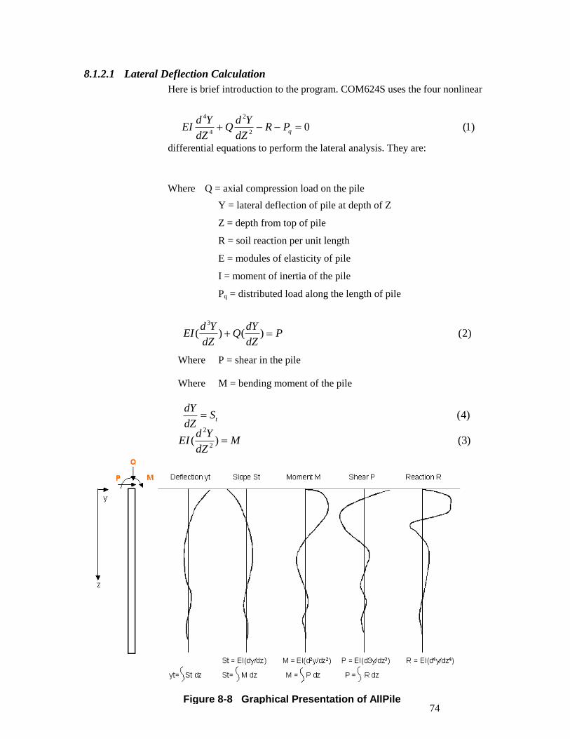
74
. . . . . . . . .
Figure 8-8 Graphical Presentation of AllPile
Results
8.1.2.1 Lateral Deflection Calculation
Here is brief introduction to the program. COM624S uses the four nonlinear
differential equations to perform the lateral analysis. They are:
Where Q = axial compression load on the pile
Y = lateral deflection of pile at depth of Z
Z = depth from top of pile
R = soil reaction per unit length
E = modules of elasticity of pile
I = moment of inertia of the pile
Pq = distributed load along the length of pile
Where P = shear in the pile
Where M = bending moment of the pile
Where St = slope of the elastic curve defined by the axis of pile
1)( 02
2
4
4
qPRdZ
YdQ
dZ
YdEI
2)( )()(3
PdZ
dYQ
dZ
YdEI
)3( )(2
2
MdZ
YdEI
)4( tSdZ
dY
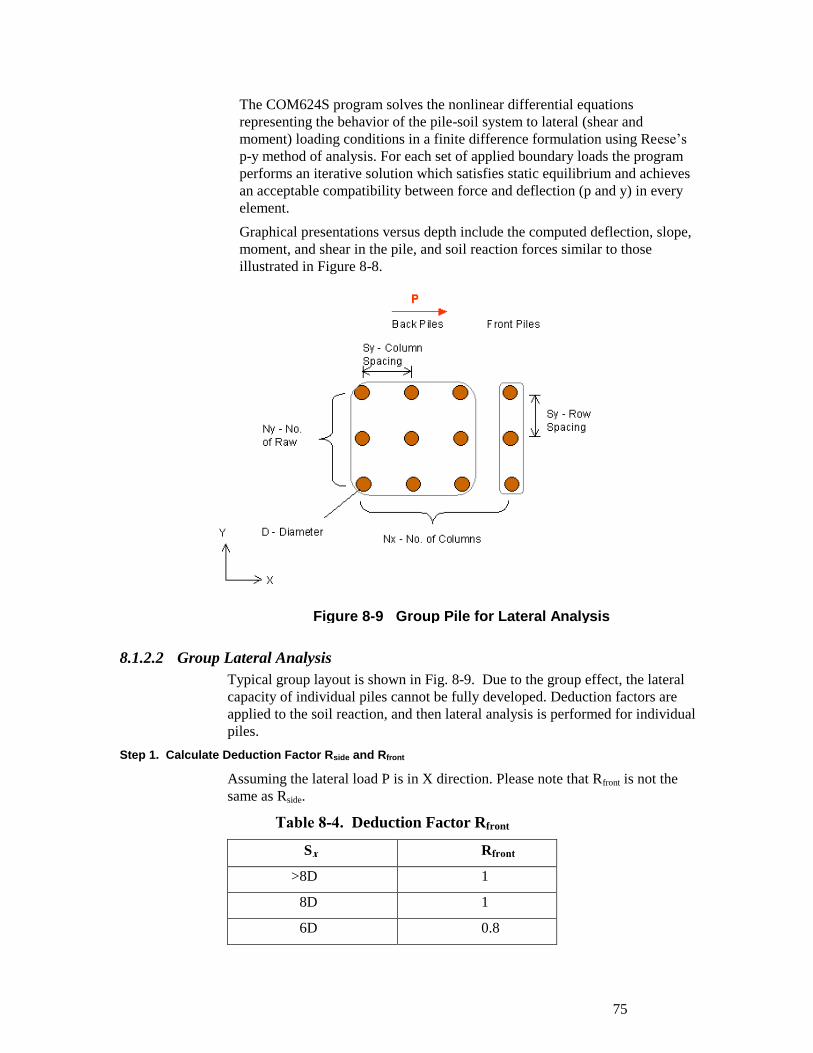
75
. . . . . . . . .
Figure 8-9 Group Pile for Lateral Analysis
The COM624S program solves the nonlinear differential equations
representing the behavior of the pile-soil system to lateral (shear and
moment) loading conditions in a finite difference formulation using Reese’s
p-y method of analysis. For each set of applied boundary loads the program
performs an iterative solution which satisfies static equilibrium and achieves
an acceptable compatibility between force and deflection (p and y) in every
element.
Graphical presentations versus depth include the computed deflection, slope,
moment, and shear in the pile, and soil reaction forces similar to those
illustrated in Figure 8-8.
8.1.2.2 Group Lateral Analysis
Typical group layout is shown in Fig. 8-9. Due to the group effect, the lateral
capacity of individual piles cannot be fully developed. Deduction factors are
applied to the soil reaction, and then lateral analysis is performed for individual
piles.
Step 1. Calculate Deduction Factor Rside and Rfront
Assuming the lateral load P is in X direction. Please note that Rfront is not the
same as Rside.
Table 8-4. Deduction Factor Rfront
Sx Rfront
>8D 1
8D 1
6D 0.8
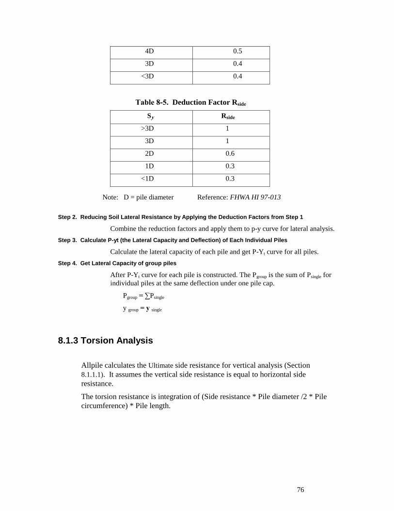
76
. . . . . . . . .
4D 0.5
3D 0.4
<3D 0.4
Table 8-5. Deduction Factor Rside
Sy Rside
>3D 1
3D 1
2D 0.6
1D 0.3
<1D 0.3
Note: D = pile diameter Reference: FHWA HI 97-013
Step 2. Reducing Soil Lateral Resistance by Applying the Deduction Factors from Step 1
Combine the reduction factors and apply them to p-y curve for lateral analysis.
Step 3. Calculate P-yt (the Lateral Capacity and Deflection) of Each Individual Piles
Calculate the lateral capacity of each pile and get P-Yt curve for all piles.
Step 4. Get Lateral Capacity of group piles
After P-Yt curve for each pile is constructed. The Pgroup is the sum of Psingle for
individual piles at the same deflection under one pile cap.
Pgroup = ∑Psingle
y group = y single
8.1.3 Torsion Analysis
Allpile calculates the Ultimate side resistance for vertical analysis (Section
8.1.1.1). It assumes the vertical side resistance is equal to horizontal side
resistance.
The torsion resistance is integration of (Side resistance * Pile diameter /2 * Pile
circumference) * Pile length.
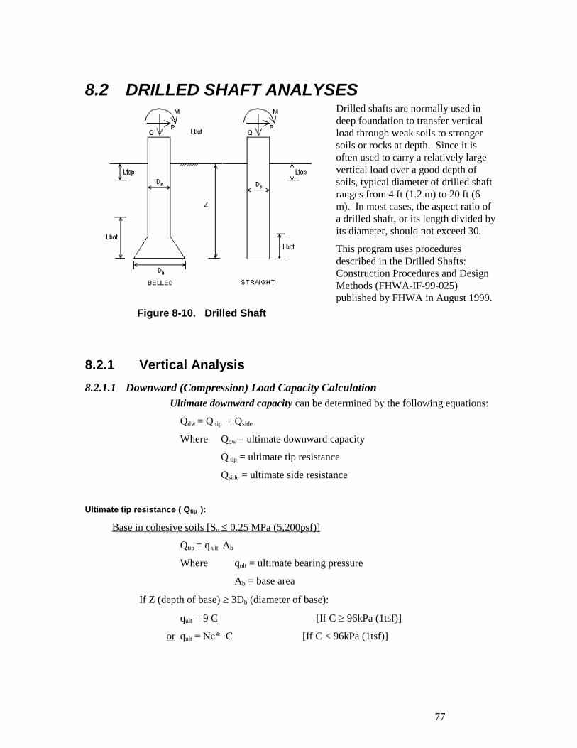
77
. . . . . . . . .
8.2 DRILLED SHAFT ANALYSES Drilled shafts are normally used in
deep foundation to transfer vertical
load through weak soils to stronger
soils or rocks at depth. Since it is
often used to carry a relatively large
vertical load over a good depth of
soils, typical diameter of drilled shaft
ranges from 4 ft (1.2 m) to 20 ft (6
m). In most cases, the aspect ratio of
a drilled shaft, or its length divided by
its diameter, should not exceed 30.
This program uses procedures
described in the Drilled Shafts:
Construction Procedures and Design
Methods (FHWA-IF-99-025)
published by FHWA in August 1999.
8.2.1 Vertical Analysis
8.2.1.1 Downward (Compression) Load Capacity Calculation
Ultimate downward capacity can be determined by the following equations:
Qdw = Q tip + Qside
Where Qdw = ultimate downward capacity
Q tip = ultimate tip resistance
Qside = ultimate side resistance
Ultimate tip resistance ( Qtip ):
Base in cohesive soils [Su 0.25 MPa (5,200psf)]
Qtip = q ult Ab
Where qult = ultimate bearing pressure
Ab = base area
If Z (depth of base) 3Db (diameter of base):
qult = 9 C [If C 96kPa (1tsf)]
or qult = Nc* ∙C [If C < 96kPa (1tsf)]
Figure 8-10. Drilled Shaft
78
. . . . . . . . .
Where C (or Sv) = undrained shear strength below base
Nc* = modified bearing capacity factor for cohesive soils. It
can be assumed to be a function of Su in UU triaxial
compression as shown in Table 8-6.
Table 8-6. Modified Bearing Capacity Factor, Nc*
C
(Undrained Shear Strength)
Nc*
(Bearing Capacity Factor)
24kPa (500psf) 6.5
48kPa (1000psf) 8.0
96kPa (2000psf) 9.0
If Z (depth of base) < 3Db (diameter of base):
Base in cohesionless soils (NSPT 50)
In Metric unit: qult (kPa) = 57.5 ∙ NSPT
In English unit: qult (tsf) = 0.6 ∙ NSPT
Where NSPT = blow count per 0.3m or 1ft of penetration in the Standard
Penetration Test. If N>51, 50 is used.
Base in rocks [0.25MPa (2.5tsf) < C < 2.5MPa (25tsf)]
If embedment in rock 1.5B (diameter of base):
qult = 5 ∙ C = 2.5 ∙ qu
If embedment in rock < 1.5B (diameter of base):
qult = 4 ∙ C = 2.0 ∙ qu
Where qu = unconfined compressive strength below base
*Attention: The two equations above were developed for drilled shafts sitting on or
embedded in good quality bedrock with RQD close to 100%. If rock is jointed or fractured,
please consult geotechnical engineer for correct procedures to calculate tip resistance.
Ultimate side resistance ( Qside ):
Q side = f0 ∙ l ∙ Pi
uc
b
ult SND
Zq
*
61
3
2
79
. . . . . . . . .
Where f0 = skin friction
l = segment of pile
Pi = perimeter of pile
Shaft in cohesive soils [Su 0.25 MPa (5,200psf)]
f0 = ∙ C
= 0.55 (for Su / Pa 1.5)
(for 1.5 Su / Pa 2.5)
Where = shear strength reduction factor
Pa = atmospheric pressure = 101kPa or 2.12ksf
Shaft in cohesionless soils (NSPT 50)
f0 = ∙ C
In sand:
= 1.5 - 0.245 [Z(m)]0.5
[If NSPT 15 B/0.3m]
or = NSPT /15 ∙ {1.5 - 0.245 [Z(m)]0.5
} [If NSPT < 15 B/0.3m]
Where = empirical factor which varies with depth
Sv = effective vertical stress at depth Z
Z = depth where side resistance is calculated
Attention: - Z must be converted to meter before calculating .
- Range of : 0.25 1.2
Shaft in rocks [0.25MPa (2.5tsf) < C < 2.5MPa (25tsf)]
Where qu = unconfined compressive strength at depth where side
resistance is calculated
Pa = atmospheric pressure = 101kPa or 2.12ksf
8.2.1.2 Uplift Load Capacity Calculation
Ultimate uplift capacity can be determined by the following equations:
Qup = Qw + Q'side + Q'b
5.11.055.0
a
u
P
S
5.0
0q
65.0f
a
ua
PP
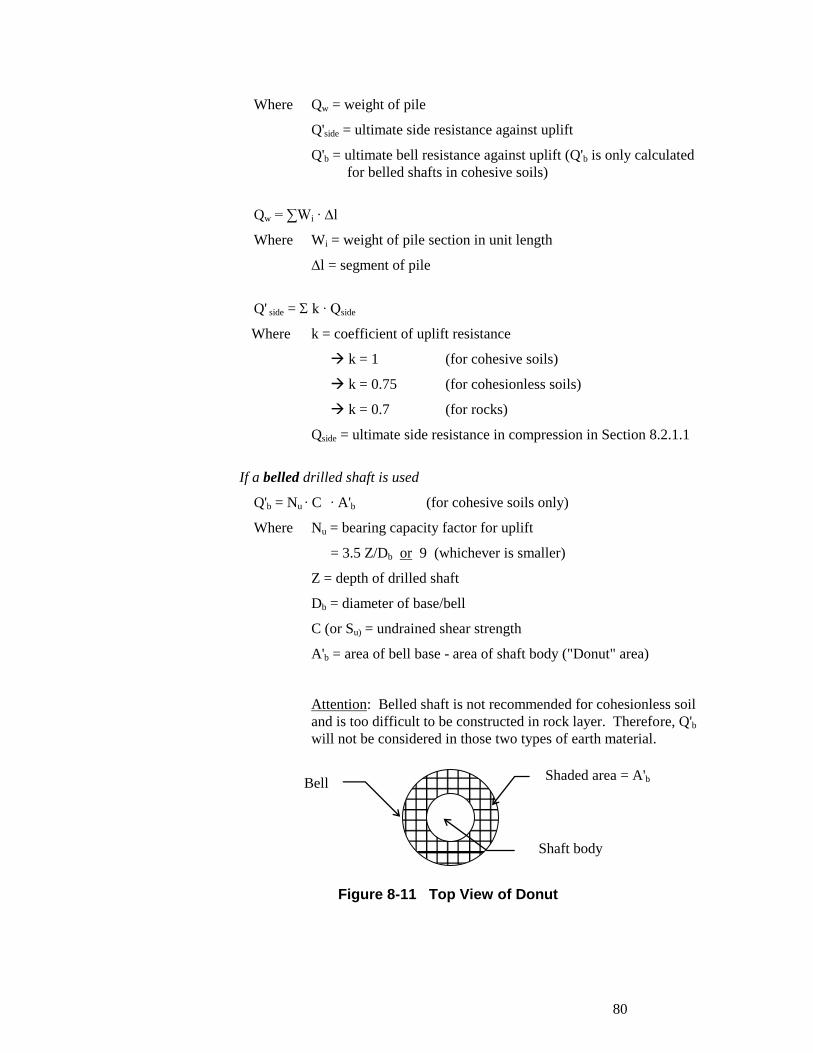
80
. . . . . . . . .
Where Qw = weight of pile
Q'side = ultimate side resistance against uplift
Q'b = ultimate bell resistance against uplift (Q'b is only calculated
for belled shafts in cohesive soils)
Qw = ∑Wi ∙ ∆l
Where Wi = weight of pile section in unit length
∆l = segment of pile
Q' side = k ∙ Qside
Where k = coefficient of uplift resistance
k = 1 (for cohesive soils)
k = 0.75 (for cohesionless soils)
k = 0.7 (for rocks)
Qside = ultimate side resistance in compression in Section 8.2.1.1
If a belled drilled shaft is used
Q'b = Nu ∙ C ∙ A'b (for cohesive soils only)
Where Nu = bearing capacity factor for uplift
= 3.5 Z/Db or 9 (whichever is smaller)
Z = depth of drilled shaft
Db = diameter of base/bell
C (or Su) = undrained shear strength
A'b = area of bell base - area of shaft body ("Donut" area)
Attention: Belled shaft is not recommended for cohesionless soil
and is too difficult to be constructed in rock layer. Therefore, Q'b
will not be considered in those two types of earth material.
Shaded area = A'b
Figure 8-11 Top View of Donut
Shaft body
Bell Shaded area = A'b
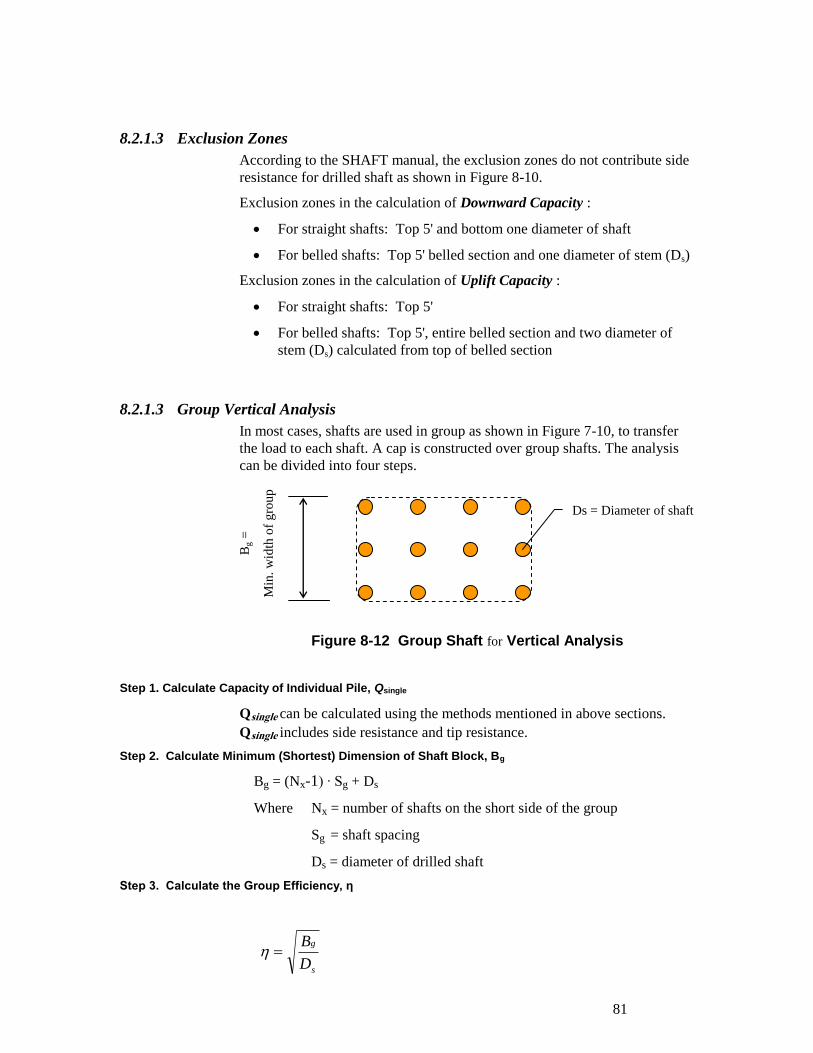
81
. . . . . . . . .
8.2.1.3 Exclusion Zones
According to the SHAFT manual, the exclusion zones do not contribute side
resistance for drilled shaft as shown in Figure 8-10.
Exclusion zones in the calculation of Downward Capacity :
For straight shafts: Top 5' and bottom one diameter of shaft
For belled shafts: Top 5' belled section and one diameter of stem (Ds)
Exclusion zones in the calculation of Uplift Capacity :
For straight shafts: Top 5'
For belled shafts: Top 5', entire belled section and two diameter of
stem (Ds) calculated from top of belled section
8.2.1.3 Group Vertical Analysis
In most cases, shafts are used in group as shown in Figure 7-10, to transfer
the load to each shaft. A cap is constructed over group shafts. The analysis
can be divided into four steps.
Figure 8-12 Group Shaft for Vertical Analysis
Step 1. Calculate Capacity of Individual Pile, Qsingle
Qsingle can be calculated using the methods mentioned in above sections.
Qsingle includes side resistance and tip resistance.
Step 2. Calculate Minimum (Shortest) Dimension of Shaft Block, Bg
Bg = (Nx-1) ∙ Sg + Ds
Where Nx = number of shafts on the short side of the group
Sg = shaft spacing
Ds = diameter of drilled shaft
Step 3. Calculate the Group Efficiency, η
s
g
D
B
Bg =
Min
. w
idth
of
gro
up
Ds = Diameter of shaft
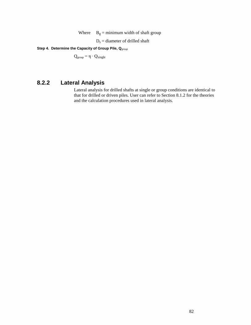
82
. . . . . . . . .
Where Bg = minimum width of shaft group
Ds = diameter of drilled shaft
Step 4. Determine the Capacity of Group Pile, Qgroup
Qgroup = η ∙ Qsingle
8.2.2 Lateral Analysis
Lateral analysis for drilled shafts at single or group conditions are identical to
that for drilled or driven piles. User can refer to Section 8.1.2 for the theories
and the calculation procedures used in lateral analysis.
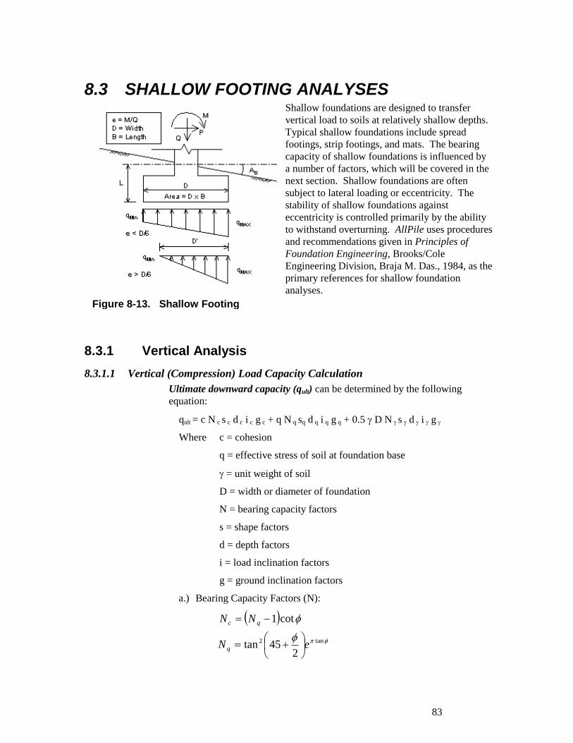
83
. . . . . . . . .
Figure 8-13. Shallow Footing
8.3 SHALLOW FOOTING ANALYSES Shallow foundations are designed to transfer
vertical load to soils at relatively shallow depths.
Typical shallow foundations include spread
footings, strip footings, and mats. The bearing
capacity of shallow foundations is influenced by
a number of factors, which will be covered in the
next section. Shallow foundations are often
subject to lateral loading or eccentricity. The
stability of shallow foundations against
eccentricity is controlled primarily by the ability
to withstand overturning. AllPile uses procedures
and recommendations given in Principles of
Foundation Engineering, Brooks/Cole
Engineering Division, Braja M. Das., 1984, as the
primary references for shallow foundation
analyses.
8.3.1 Vertical Analysis
8.3.1.1 Vertical (Compression) Load Capacity Calculation
Ultimate downward capacity (qult) can be determined by the following
equation:
qult = c N c s c d c i c g c + q N q sq d q i q g q + 0.5 D N s d i g
Where c = cohesion
q = effective stress of soil at foundation base
= unit weight of soil
D = width or diameter of foundation
N = bearing capacity factors
s = shape factors
d = depth factors
i = load inclination factors
g = ground inclination factors
a.) Bearing Capacity Factors (N):
2
45tan tan2 eN q
cot1 qc NN
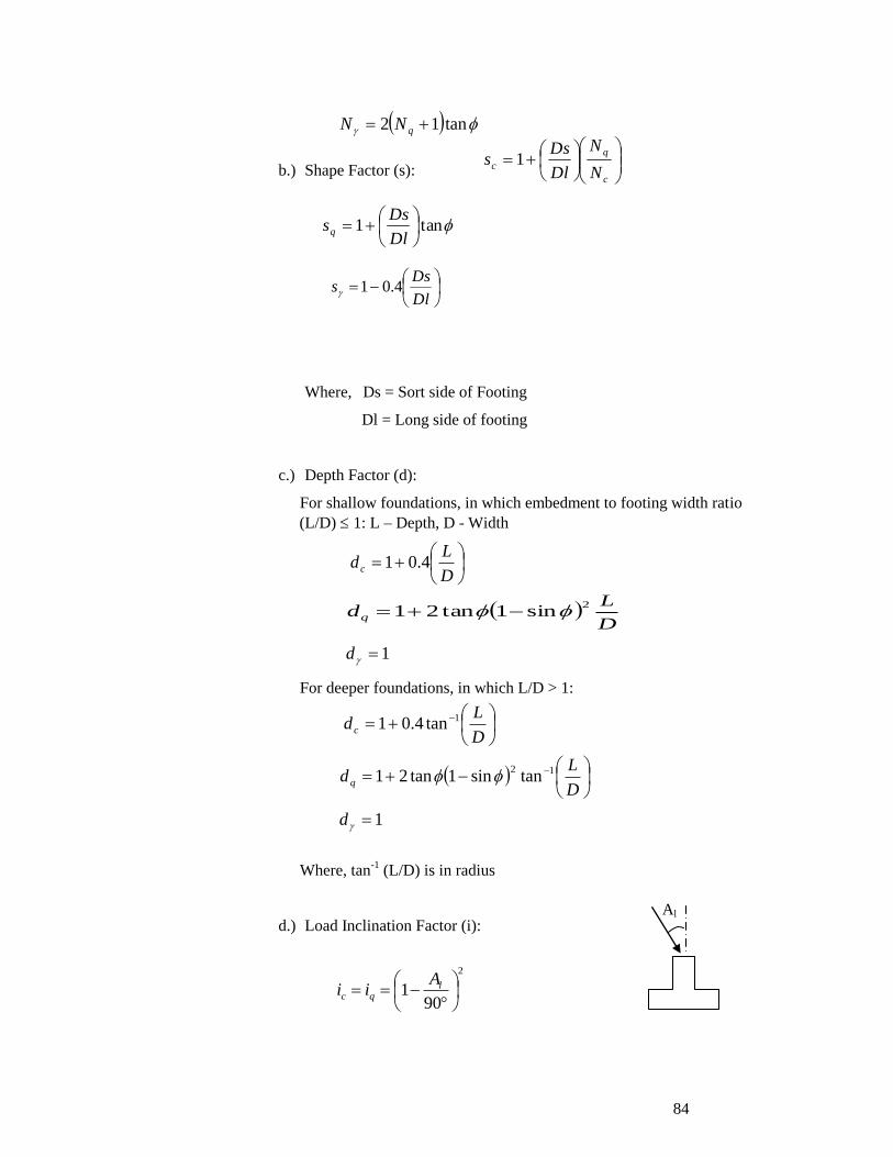
84
. . . . . . . . .
tan12 qNN
D
Ldc
1tan4.01
D
Ldc 4.01
D
Ldq
2sin1tan21
b.) Shape Factor (s):
Where, Ds = Sort side of Footing
Dl = Long side of footing
c.) Depth Factor (d):
For shallow foundations, in which embedment to footing width ratio
(L/D) 1: L – Depth, D - Width
For deeper foundations, in which L/D > 1:
Where, tan-1
(L/D) is in radius
d.) Load Inclination Factor (i):
D
Ld q
12tansin1tan21
1d
2
901
l
qc
Aii
1d
Al
c
q
cN
N
Dl
Dss 1
tan1
Dl
Dssq
Dl
Dss 4.01
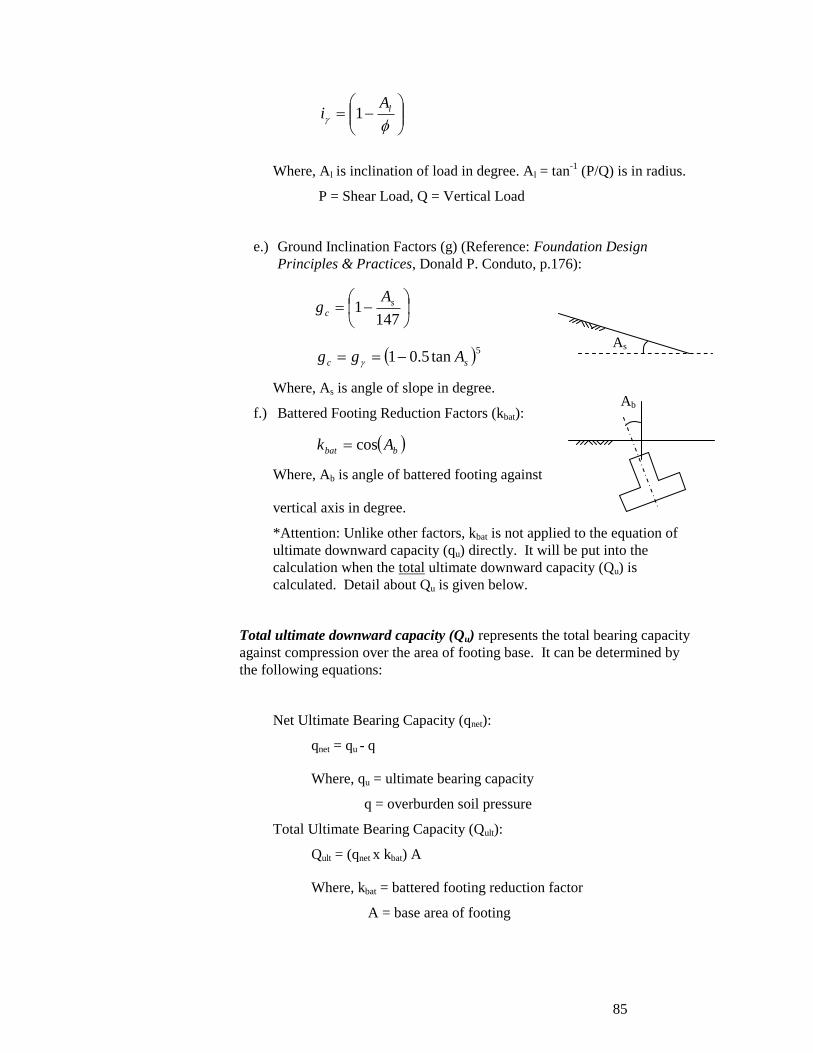
85
. . . . . . . . .
Where, Al is inclination of load in degree. Al = tan-1
(P/Q) is in radius.
P = Shear Load, Q = Vertical Load
e.) Ground Inclination Factors (g) (Reference: Foundation Design
Principles & Practices, Donald P. Conduto, p.176):
Where, As is angle of slope in degree.
f.) Battered Footing Reduction Factors (kbat):
Where, Ab is angle of battered footing against
vertical axis in degree.
*Attention: Unlike other factors, kbat is not applied to the equation of
ultimate downward capacity (qu) directly. It will be put into the
calculation when the total ultimate downward capacity (Qu) is
calculated. Detail about Qu is given below.
Total ultimate downward capacity (Qu) represents the total bearing capacity
against compression over the area of footing base. It can be determined by
the following equations:
Net Ultimate Bearing Capacity (qnet):
qnet = qu - q
Where, qu = ultimate bearing capacity
q = overburden soil pressure
Total Ultimate Bearing Capacity (Qult):
Qult = (qnet x kbat) A
Where, kbat = battered footing reduction factor
A = base area of footing
As
lA
i 1
1471 s
c
Ag
5tan5.01 sc Agg
bbat Ak cos
Ab
86
. . . . . . . . .
Allowable downward capacity (Qallow) can be calculated by the following
equation:
8.3.2 Capacity for Combined Loading
8.3.2.1 Vertical (Compression) Load (Q) Only
If there is only a vertical load, Q, without any lateral loading, i.e. shear loads
and bending moment, the Factor of Safety of the shallow foundation can be
calculated using the equation below:
Where, Qult = ultimate bearing capacity
Q = total vertical load
Users can also check the ratio between Q and the allowable bearing capacity,
Qallow, to see if the shallow foundation is considered stable. If Q > Qallow, the
foundation is insufficient.
8.3.2.2 Vertical Load With Moment (Q + M)
Typical lateral loads on the foundation include bending moment (M) and
shear load (P) as illustrated in the next diagram. In this section, we will study
the procedures used to determine footing capacity against the combination of
vertical load and bending moment (Q+M).
Eccentricity (e) will be generated by the moment and vertical load (see Figure
8-12):
a.) If e D/6, the pressure on the foundation can be determined by:
..SF
ult
allow
...
Q
QSF
ult
Q
Me
BD
M
DB
2max
6
BD
M
DB
2min
6
87
. . . . . . . . .
Where, D = width of foundation base in lateral load direction
B = length of foundation base in the other direction
Reaction pressure at the base of the foundation distributed in a trapezoid
pattern across the full width (D) of the foundation.
b.) If e > D/6, then:
Reaction pressure at the base of the foundation is distributed in a triangular
pattern across the effective width (D') of the foundation.
Due to the distribution of reaction pressure, a new ultimate bearing
capacity called, qult', has to be recalculated using the same procedures as
mentioned in Section 8.3.1.1, but based on D' instead of D.
To calculate the Factor of Safety:
or
Where, Qult' = qult' D' B
8.3.2.3 Vertical Load With Shear Load (Q + P)
The shear load (P) has two impacts to the shallow foundation calculation:
1. It generates load inclination Al = tan-1
(P/Q) which affects vertical
bearing capacity calculation (see Section 8.3.1.1).
2. Footing base sliding calculation becomes necessary. The sliding
resistance (Pf) can be calculated by the following equation:
0min q
eDB
24
4max
eDD 2'
max
'..
q
qSF
ult
Q
QSF
ult '..
)( QWkP ff
88
. . . . . . . . .
Where, kf = base friction factor for cast-in-place foundation
kf is close to tan ( = angle of internal friction)
kf = 0.3-0.8 is recommended
W = weight of footing and the soil above
Factor of Safety against sliding can be calculated by:
8.3.3 Settlement From Vertical Load If only vertical load is applied to the shallow foundation, the elastic
settlement (X0) of the footing can be calculated using the equation below:
Where, q0 = pressure under working load
Ds – Short side of footing
Dl – Long side of footing
- Poisson ratio; = 0.3 is recommended for general
soil conditions
Es - Young's modulus
Es = 766NSPT for cohesionless soils
Es = 375C for cohesive soils
Where, NSPT = blow count over 12" of soil
C = undrained cohesion of soil
= Settlement factor for flexible foundation, which is a
function of Dl/Ds (footing shape ratio)
[Note 1] X0 is the elastic settlement at the center of a footing. If there is soft
clay underneath the footing, consolidation settlement, which is time-
dependent, should be considered. AllPile does not include calculation of
consolidation settlement as it is not within the scope of the program.
[Note 2] AllPile assumes that a hard layer of soil, i.e. rock or intermediate
geomaterials (IGMs) is in great depth from the base of footing. If Ha, the
distance between footing base and hard soil, is over 4 times the footing width
(D), the actual elastic settlement will not change considerably.
If Ha is less than 4D, the elastic settlement can be calculated based on the
following equation:
P
PSF
f..
)4(4
' 00 a
a HD
HXX
)1( 20
0
sE
DsqX
..00
SF
qqor
Area
Qq u
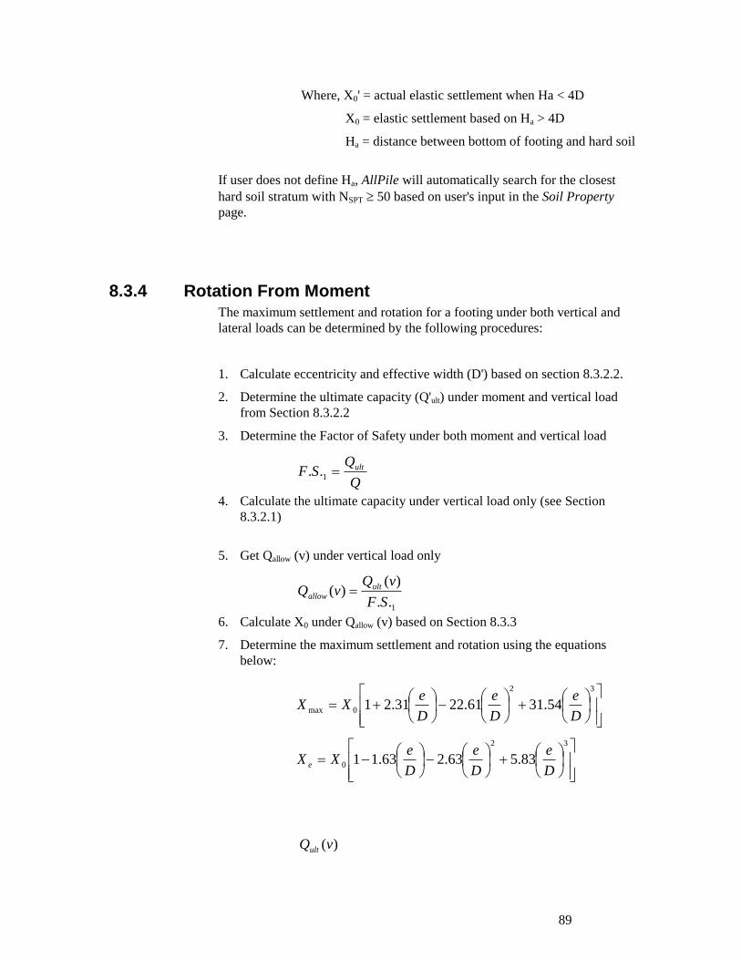
89
. . . . . . . . .
Where, X0' = actual elastic settlement when Ha < 4D
X0 = elastic settlement based on Ha > 4D
Ha = distance between bottom of footing and hard soil
If user does not define Ha, AllPile will automatically search for the closest
hard soil stratum with NSPT 50 based on user's input in the Soil Property
page.
8.3.4 Rotation From Moment The maximum settlement and rotation for a footing under both vertical and
lateral loads can be determined by the following procedures:
1. Calculate eccentricity and effective width (D') based on section 8.3.2.2.
2. Determine the ultimate capacity (Q'ult) under moment and vertical load
from Section 8.3.2.2
3. Determine the Factor of Safety under both moment and vertical load
4. Calculate the ultimate capacity under vertical load only (see Section
8.3.2.1)
5. Get Qallow (v) under vertical load only
6. Calculate X0 under Qallow (v) based on Section 8.3.3
7. Determine the maximum settlement and rotation using the equations
below:
Q
QSF ult1..
1..
)()(
SF
vQvQ ult
allow
)(vQult
32
0max 54.3161.2231.21D
e
D
e
D
eXX
32
0 83.563.263.11D
e
D
e
D
eXX e
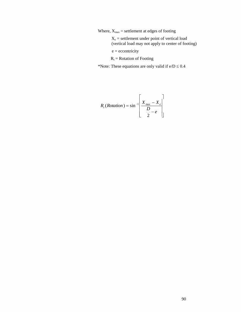
90
. . . . . . . . .
Where, Xmax = settlement at edges of footing
Xe = settlement under point of vertical load
(vertical load may not apply to center of footing)
e = eccentricity
Rt = Rotation of Footing
*Note: These equations are only valid if e/D 0.4
eD
XXRotationR e
t
2
sin)( max1
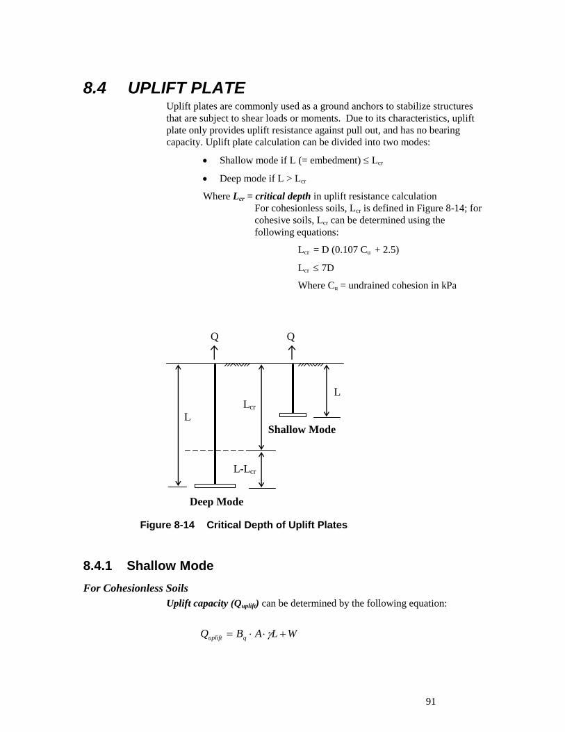
91
. . . . . . . . .
8.4 UPLIFT PLATE Uplift plates are commonly used as a ground anchors to stabilize structures
that are subject to shear loads or moments. Due to its characteristics, uplift
plate only provides uplift resistance against pull out, and has no bearing
capacity. Uplift plate calculation can be divided into two modes:
Shallow mode if L (= embedment) Lcr
Deep mode if L > Lcr
Where Lcr = critical depth in uplift resistance calculation
For cohesionless soils, Lcr is defined in Figure 8-14; for
cohesive soils, Lcr can be determined using the
following equations:
Lcr = D (0.107 Cu + 2.5)
Lcr 7D
Where Cu = undrained cohesion in kPa
8.4.1 Shallow Mode
For Cohesionless Soils
Uplift capacity (Quplift) can be determined by the following equation:
WLABQ quplift
L-Lcr
Lcr L
L
Deep Mode
Shallow Mode
Q Q
Figure 8-14 Critical Depth of Uplift Plates
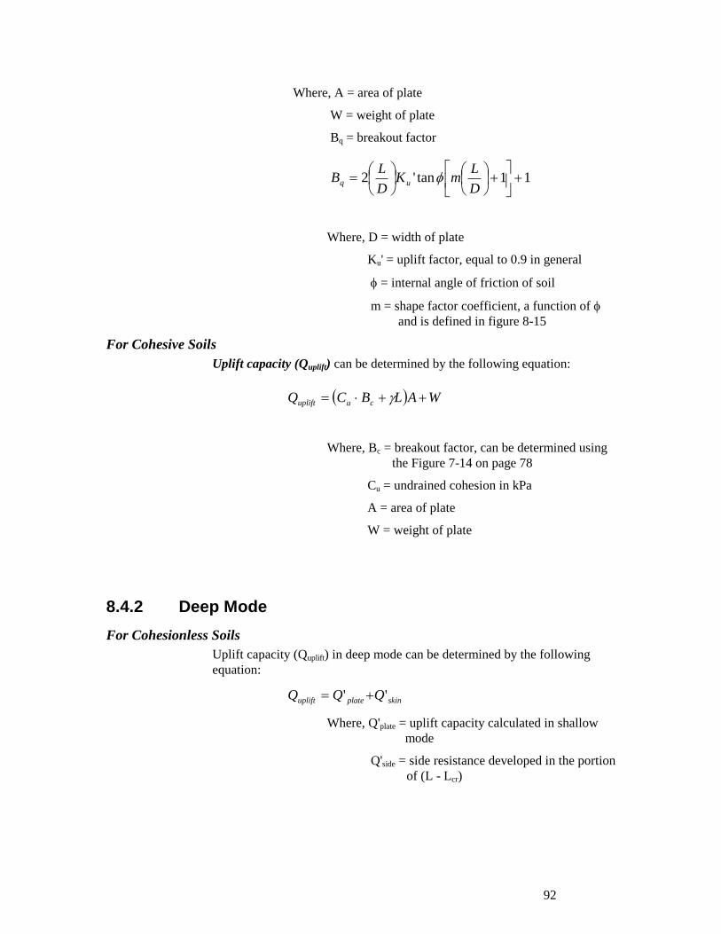
92
. . . . . . . . .
Where, A = area of plate
W = weight of plate
Bq = breakout factor
Where, D = width of plate
Ku' = uplift factor, equal to 0.9 in general
= internal angle of friction of soil
m = shape factor coefficient, a function of
and is defined in figure 8-15
For Cohesive Soils
Uplift capacity (Quplift) can be determined by the following equation:
Where, Bc = breakout factor, can be determined using
the Figure 7-14 on page 78
Cu = undrained cohesion in kPa
A = area of plate
W = weight of plate
8.4.2 Deep Mode
For Cohesionless Soils
Uplift capacity (Quplift) in deep mode can be determined by the following
equation:
Where, Q'plate = uplift capacity calculated in shallow
mode
Q'side = side resistance developed in the portion
of (L - Lcr)
11tan'2
D
LmK
D
LB uq
WALBCQ cuuplift
skinplateuplift QQQ ''
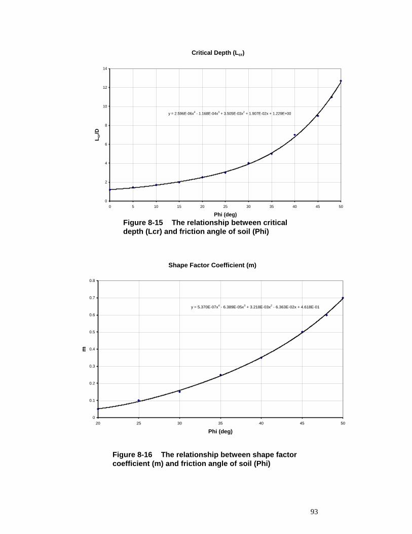
93
. . . . . . . . .
Critical Depth (Lcr)
y = 2.596E-06x4 - 1.168E-04x
3 + 3.505E-03x
2 + 1.907E-02x + 1.229E+00
0
2
4
6
8
10
12
14
0 5 10 15 20 25 30 35 40 45 50
Phi (deg)
Lcr/D
Figure 8-15 The relationship between critical
depth (Lcr) and friction angle of soil (Phi)
Shape Factor Coefficient (m)
y = 5.370E-07x4 - 6.389E-05x
3 + 3.218E-03x
2 - 6.363E-02x + 4.618E-01
0
0.1
0.2
0.3
0.4
0.5
0.6
0.7
0.8
20 25 30 35 40 45 50
Phi (deg)
m
Figure 8-16 The relationship between shape factor
coefficient (m) and friction angle of soil (Phi)
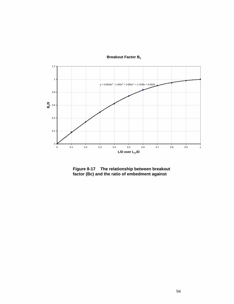
94
. . . . . . . . .
Breakout Factor Bc
y = 0.6818x4 - 1.493x
3 + 0.085x
2 + 1.7209x + 0.0034
0
0.2
0.4
0.6
0.8
1
1.2
0 0.1 0.2 0.3 0.4 0.5 0.6 0.7 0.8 0.9 1
L/D over Lcr/D
Bc/9
Figure 8-17 The relationship between breakout
factor (Bc) and the ratio of embedment against
critical depth
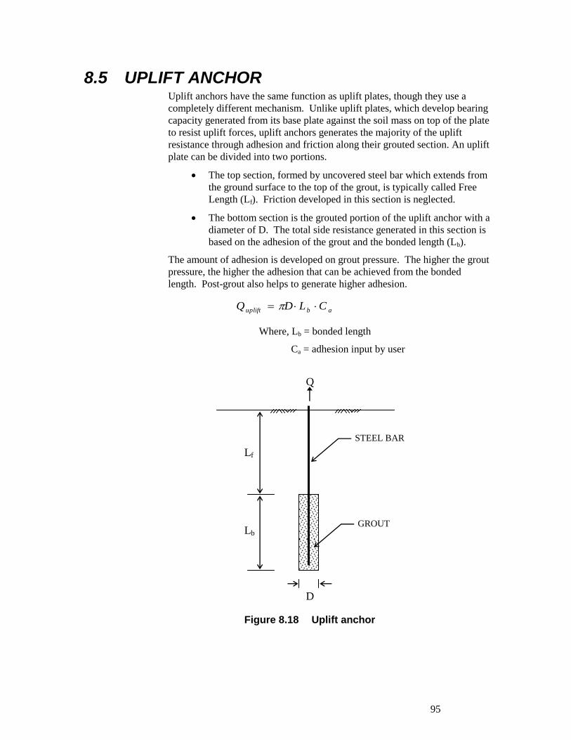
95
. . . . . . . . .
8.5 UPLIFT ANCHOR Uplift anchors have the same function as uplift plates, though they use a
completely different mechanism. Unlike uplift plates, which develop bearing
capacity generated from its base plate against the soil mass on top of the plate
to resist uplift forces, uplift anchors generates the majority of the uplift
resistance through adhesion and friction along their grouted section. An uplift
plate can be divided into two portions.
The top section, formed by uncovered steel bar which extends from
the ground surface to the top of the grout, is typically called Free
Length (Lf). Friction developed in this section is neglected.
The bottom section is the grouted portion of the uplift anchor with a
diameter of D. The total side resistance generated in this section is
based on the adhesion of the grout and the bonded length (Lb).
The amount of adhesion is developed on grout pressure. The higher the grout
pressure, the higher the adhesion that can be achieved from the bonded
length. Post-grout also helps to generate higher adhesion.
Where, Lb = bonded length
Ca = adhesion input by user
abuplift CLDQ
Lf
Lb
D
Q
GROUT
STEEL BAR
Figure 8.18 Uplift anchor
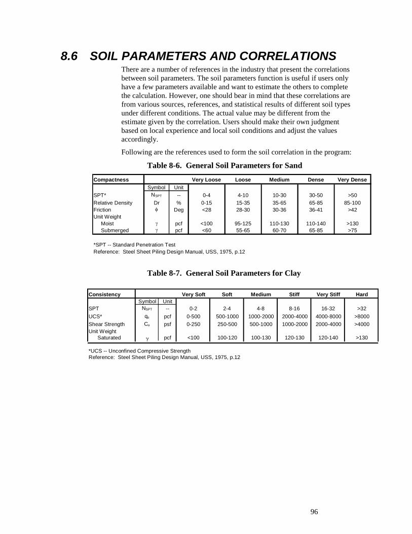
96
. . . . . . . . .
8.6 SOIL PARAMETERS AND CORRELATIONS There are a number of references in the industry that present the correlations
between soil parameters. The soil parameters function is useful if users only
have a few parameters available and want to estimate the others to complete
the calculation. However, one should bear in mind that these correlations are
from various sources, references, and statistical results of different soil types
under different conditions. The actual value may be different from the
estimate given by the correlation. Users should make their own judgment
based on local experience and local soil conditions and adjust the values
accordingly.
Following are the references used to form the soil correlation in the program:
Table 8-6. General Soil Parameters for Sand
Table 8-7. General Soil Parameters for Clay
Compactness Very Loose Loose Medium Dense Very Dense
Symbol Unit
SPT* NSPT -- 0-4 4-10 10-30 30-50 >50
Relative Density Dr % 0-15 15-35 35-65 65-85 85-100
Friction Deg <28 28-30 30-36 36-41 >42
Unit Weight
Moist pcf <100 95-125 110-130 110-140 >130
Submerged pcf <60 55-65 60-70 65-85 >75
*SPT -- Standard Penetration Test
Reference: Steel Sheet Piling Design Manual, USS, 1975, p.12
Consistency Very Soft Soft Medium Stiff Very Stiff Hard
Symbol Unit
SPT NSPT -- 0-2 2-4 4-8 8-16 16-32 >32
UCS* qu pcf 0-500 500-1000 1000-2000 2000-4000 4000-8000 >8000
Shear Strength Cu psf 0-250 250-500 500-1000 1000-2000 2000-4000 >4000
Unit Weight
Saturated pcf <100 100-120 100-130 120-130 120-140 >130
*UCS -- Unconfined Compressive Strength
Reference: Steel Sheet Piling Design Manual, USS, 1975, p.12
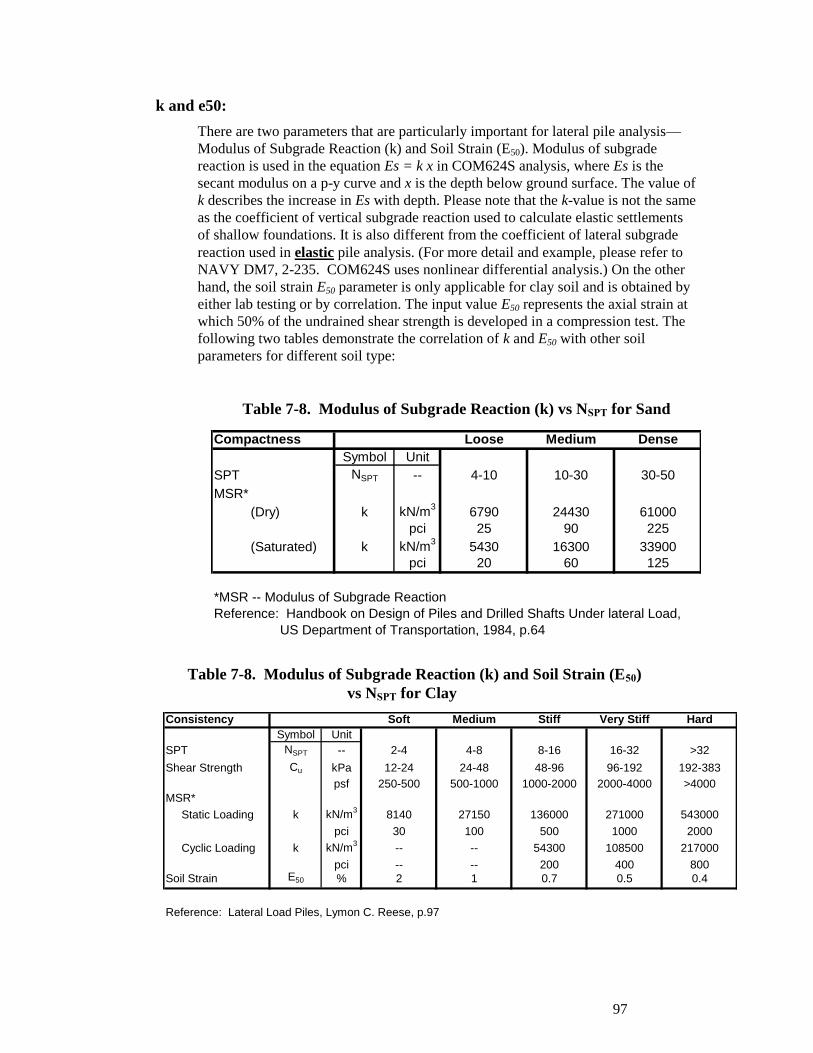
97
. . . . . . . . .
k and e50:
There are two parameters that are particularly important for lateral pile analysis—
Modulus of Subgrade Reaction (k) and Soil Strain (E50). Modulus of subgrade
reaction is used in the equation Es = k x in COM624S analysis, where Es is the
secant modulus on a p-y curve and x is the depth below ground surface. The value of
k describes the increase in Es with depth. Please note that the k-value is not the same
as the coefficient of vertical subgrade reaction used to calculate elastic settlements
of shallow foundations. It is also different from the coefficient of lateral subgrade
reaction used in elastic pile analysis. (For more detail and example, please refer to
NAVY DM7, 2-235. COM624S uses nonlinear differential analysis.) On the other
hand, the soil strain E50 parameter is only applicable for clay soil and is obtained by
either lab testing or by correlation. The input value E50 represents the axial strain at
which 50% of the undrained shear strength is developed in a compression test. The
following two tables demonstrate the correlation of k and E50 with other soil
parameters for different soil type:
Table 7-8. Modulus of Subgrade Reaction (k) vs NSPT for Sand
Table 7-8. Modulus of Subgrade Reaction (k) and Soil Strain (E50)
vs NSPT for Clay
Compactness Loose Medium Dense
Symbol Unit
SPT NSPT -- 4-10 10-30 30-50
MSR*
(Dry) k kN/m3
6790 24430 61000
pci 25 90 225
(Saturated) k kN/m3
5430 16300 33900
pci 20 60 125
*MSR -- Modulus of Subgrade Reaction
Reference: Handbook on Design of Piles and Drilled Shafts Under lateral Load,
US Department of Transportation, 1984, p.64
Consistency Soft Medium Stiff Very Stiff Hard
Symbol Unit
SPT NSPT -- 2-4 4-8 8-16 16-32 >32
Shear Strength Cu kPa 12-24 24-48 48-96 96-192 192-383
psf 250-500 500-1000 1000-2000 2000-4000 >4000
MSR*
Static Loading k kN/m3
8140 27150 136000 271000 543000
pci 30 100 500 1000 2000
Cyclic Loading k kN/m3
-- -- 54300 108500 217000
pci -- -- 200 400 800
Soil Strain E50 % 2 1 0.7 0.5 0.4
Reference: Lateral Load Piles, Lymon C. Reese, p.97
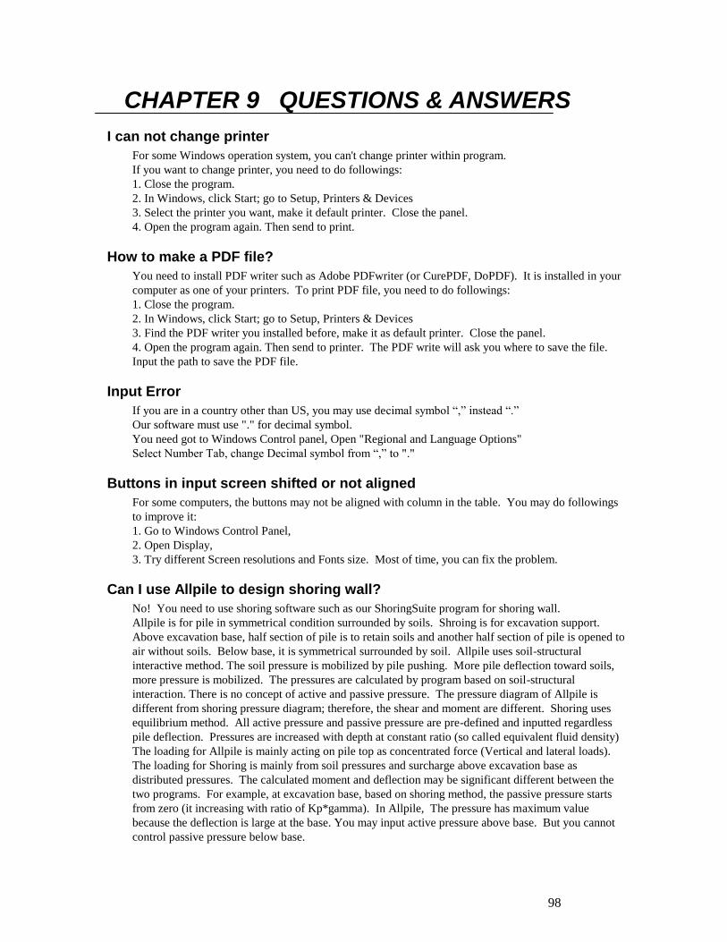
98
. . . . . . . . .
CHAPTER 9 QUESTIONS & ANSWERS
I can not change printer
For some Windows operation system, you can't change printer within program.
If you want to change printer, you need to do followings:
1. Close the program.
2. In Windows, click Start; go to Setup, Printers & Devices
3. Select the printer you want, make it default printer. Close the panel.
4. Open the program again. Then send to print.
How to make a PDF file?
You need to install PDF writer such as Adobe PDFwriter (or CurePDF, DoPDF). It is installed in your
computer as one of your printers. To print PDF file, you need to do followings:
1. Close the program.
2. In Windows, click Start; go to Setup, Printers & Devices
3. Find the PDF writer you installed before, make it as default printer. Close the panel.
4. Open the program again. Then send to printer. The PDF write will ask you where to save the file.
Input the path to save the PDF file.
Input Error
If you are in a country other than US, you may use decimal symbol “,” instead “.”
Our software must use "." for decimal symbol.
You need got to Windows Control panel, Open "Regional and Language Options"
Select Number Tab, change Decimal symbol from “,” to "."
Buttons in input screen shifted or not aligned
For some computers, the buttons may not be aligned with column in the table. You may do followings
to improve it:
1. Go to Windows Control Panel,
2. Open Display,
3. Try different Screen resolutions and Fonts size. Most of time, you can fix the problem.
Can I use Allpile to design shoring wall?
No! You need to use shoring software such as our ShoringSuite program for shoring wall.
Allpile is for pile in symmetrical condition surrounded by soils. Shroing is for excavation support.
Above excavation base, half section of pile is to retain soils and another half section of pile is opened to
air without soils. Below base, it is symmetrical surrounded by soil. Allpile uses soil-structural
interactive method. The soil pressure is mobilized by pile pushing. More pile deflection toward soils,
more pressure is mobilized. The pressures are calculated by program based on soil-structural
interaction. There is no concept of active and passive pressure. The pressure diagram of Allpile is
different from shoring pressure diagram; therefore, the shear and moment are different. Shoring uses
equilibrium method. All active pressure and passive pressure are pre-defined and inputted regardless
pile deflection. Pressures are increased with depth at constant ratio (so called equivalent fluid density)
The loading for Allpile is mainly acting on pile top as concentrated force (Vertical and lateral loads).
The loading for Shoring is mainly from soil pressures and surcharge above excavation base as
distributed pressures. The calculated moment and deflection may be significant different between the
two programs. For example, at excavation base, based on shoring method, the passive pressure starts
from zero (it increasing with ratio of Kp*gamma). In Allpile, The pressure has maximum value
because the deflection is large at the base. You may input active pressure above base. But you cannot
control passive pressure below base.
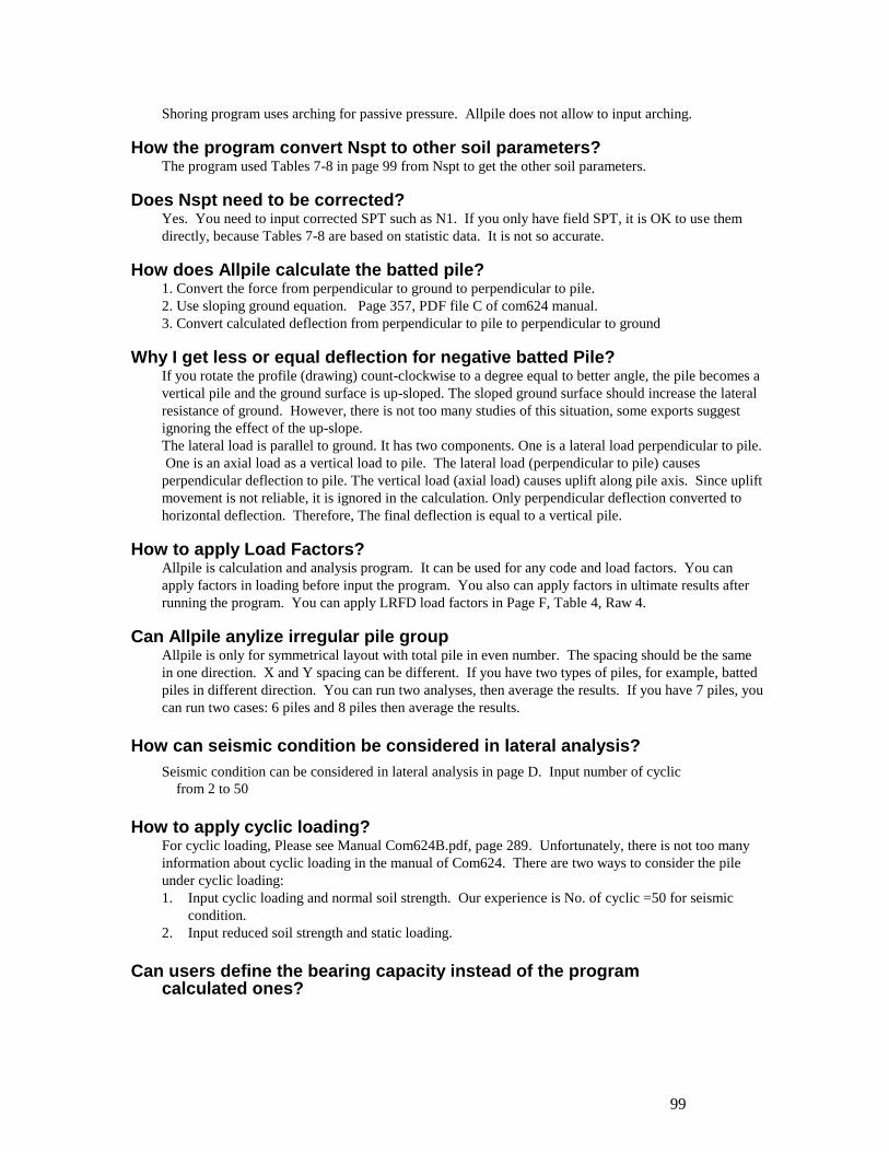
99
. . . . . . . . .
Shoring program uses arching for passive pressure. Allpile does not allow to input arching.
How the program convert Nspt to other soil parameters? The program used Tables 7-8 in page 99 from Nspt to get the other soil parameters.
Does Nspt need to be corrected?
Yes. You need to input corrected SPT such as N1. If you only have field SPT, it is OK to use them
directly, because Tables 7-8 are based on statistic data. It is not so accurate.
How does Allpile calculate the batted pile?
1. Convert the force from perpendicular to ground to perpendicular to pile.
2. Use sloping ground equation. Page 357, PDF file C of com624 manual.
3. Convert calculated deflection from perpendicular to pile to perpendicular to ground
Why I get less or equal deflection for negative batted Pile?
If you rotate the profile (drawing) count-clockwise to a degree equal to better angle, the pile becomes a
vertical pile and the ground surface is up-sloped. The sloped ground surface should increase the lateral
resistance of ground. However, there is not too many studies of this situation, some exports suggest
ignoring the effect of the up-slope.
The lateral load is parallel to ground. It has two components. One is a lateral load perpendicular to pile.
One is an axial load as a vertical load to pile. The lateral load (perpendicular to pile) causes
perpendicular deflection to pile. The vertical load (axial load) causes uplift along pile axis. Since uplift
movement is not reliable, it is ignored in the calculation. Only perpendicular deflection converted to
horizontal deflection. Therefore, The final deflection is equal to a vertical pile.
How to apply Load Factors?
Allpile is calculation and analysis program. It can be used for any code and load factors. You can
apply factors in loading before input the program. You also can apply factors in ultimate results after
running the program. You can apply LRFD load factors in Page F, Table 4, Raw 4.
Can Allpile anylize irregular pile group
Allpile is only for symmetrical layout with total pile in even number. The spacing should be the same
in one direction. X and Y spacing can be different. If you have two types of piles, for example, batted
piles in different direction. You can run two analyses, then average the results. If you have 7 piles, you
can run two cases: 6 piles and 8 piles then average the results.
How can seismic condition be considered in lateral analysis?
Seismic condition can be considered in lateral analysis in page D. Input number of cyclic
from 2 to 50
How to apply cyclic loading?
For cyclic loading, Please see Manual Com624B.pdf, page 289. Unfortunately, there is not too many
information about cyclic loading in the manual of Com624. There are two ways to consider the pile
under cyclic loading:
1. Input cyclic loading and normal soil strength. Our experience is No. of cyclic =50 for seismic
condition.
2. Input reduced soil strength and static loading.
Can users define the bearing capacity instead of the program
calculated ones?

100
. . . . . . . . .
Users can define the bearing capacity in page C. Please click Item 2, add a tip section.
Then open the pile section screen and input the bearing capacity in Item 7. Users can
also easily set bearing capacity to zero in page F, Item 2.
What are the differences between Drilled Shafts and SHAFT (US FHWA methods) in pile type?
Drilled Shafts have two types: One type is for diameters less than 24 inches; the other is for
diameters larger than 24 inches. The calculation methods are the same for both types, but the
parameters are different. Please review the parameters in Setup screen. SHAFT uses calculation
methods recommended by US FHWA. It mainly uses SPT for bearing capacity. Some side
resistances are ignored in exclusion zone. SHAFT is a more conservative method.
How many layers of soil can I input?
Up to 10 layers of soil. If you have more than 10 layers of soil, you need
to combine two or three similar layers to one layer. Here are some
examples: If you have the following layers:
2m thick with SPT=5, 3m thick with SPT=12, 1m thick with SPT=7.
You can combine them into one layer: 6m thick with
SPT=(5x2+12x3+7x1)/6=8.8
Can Allpile design the reinforcement?
No. You need to estimate the reinforcement first and input to the program, and then the program
calculate the capacity of pile and the moment in the pile. Using the Max. Moment, you can design the
reinforcement based on concrete design code. Sometime, you may need concrete design software.
There are some software can help you.
1. Enercalc http://www.enercalc.com/products.html
2. PCA software http://www.structurepoint.org/soft/soft_profile.asp?l_family_id=30
Open End Pile with Plugged CondItions
For diving pile, users can select between open-end pile and close-end pile in Page A, Item 1.
In open-end pile program uses effective area (A' - the area of steel tube) for tip resistance calculation.
In close-end pile, program uses total gross area (At - the area base on outside diameter) for tip
resistance calculation.
In both types, you always can add a tip section (Page C, Item 2), and then specify a tip area you want in
following steps:
1. Select open-end pile or close-end pile in Page A, Item 1.
2. Create a tip section in Page C, Item 2.
Input a tip area (Here we call it as A_plug).
You need estimate A_plug based on soil type, local experience and knowledge of piles.
A_plug always falls between A and A'
If pile is fully plugged, use A_plug=At
If pile is not plugged, use A_plug=A’
The easy way is using A_plug=(A+A')/2
If it is more plug and more friction inside, A_plug close to At.
If it is less plug and less friction inside, A_plug close to A'.
The side resistance calculation outside pile is the same between two types of piles.
Why the tip resistance is diffrent from my hand calulation?
You need to set Input Page F, Item 3 to zero.
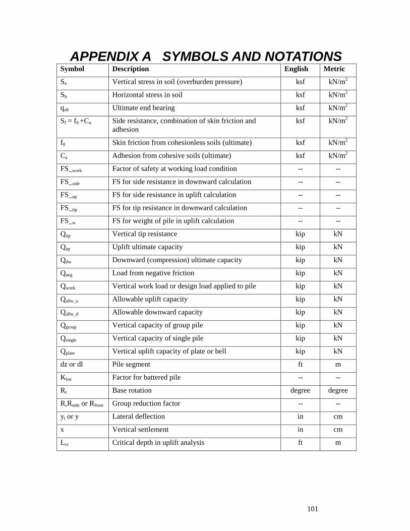
101
. . . . . . . . .
APPENDIX A SYMBOLS AND NOTATIONS
Symbol Description English Metric
Sv Vertical stress in soil (overburden pressure) ksf kN/m2
Sh Horizontal stress in soil ksf kN/m2
qult Ultimate end bearing ksf kN/m2
Sf = f0 +Ca Side resistance, combination of skin friction and
adhesion
ksf kN/m2
f0 Skin friction from cohesionless soils (ultimate) ksf kN/m2
Ca Adhesion from cohesive soils (ultimate) ksf kN/m2
FS_work Factor of safety at working load condition -- --
FS_side FS for side resistance in downward calculation -- --
FS_up FS for side resistance in uplift calculation -- --
FS_tip FS for tip resistance in downward calculation -- --
FS_w FS for weight of pile in uplift calculation -- --
Qtip Vertical tip resistance kip kN
Qup Uplift ultimate capacity kip kN
Qdw Downward (compression) ultimate capacity kip kN
Qneg Load from negative friction kip kN
Qwork Vertical work load or design load applied to pile kip kN
Qallw_u Allowable uplift capacity kip kN
Qallw_d Allowable downward capacity kip kN
Qgroup Vertical capacity of group pile kip kN
Qsingle Vertical capacity of single pile kip kN
Qplate Vertical uplift capacity of plate or bell kip kN
dz or dl Pile segment ft m
Kbat Factor for battered pile -- --
Rt Base rotation degree degree
R,Rside or Rfront Group reduction factor -- --
yt or y Lateral deflection in cm
x Vertical settlement in cm
Lcr Critical depth in uplift analysis ft m
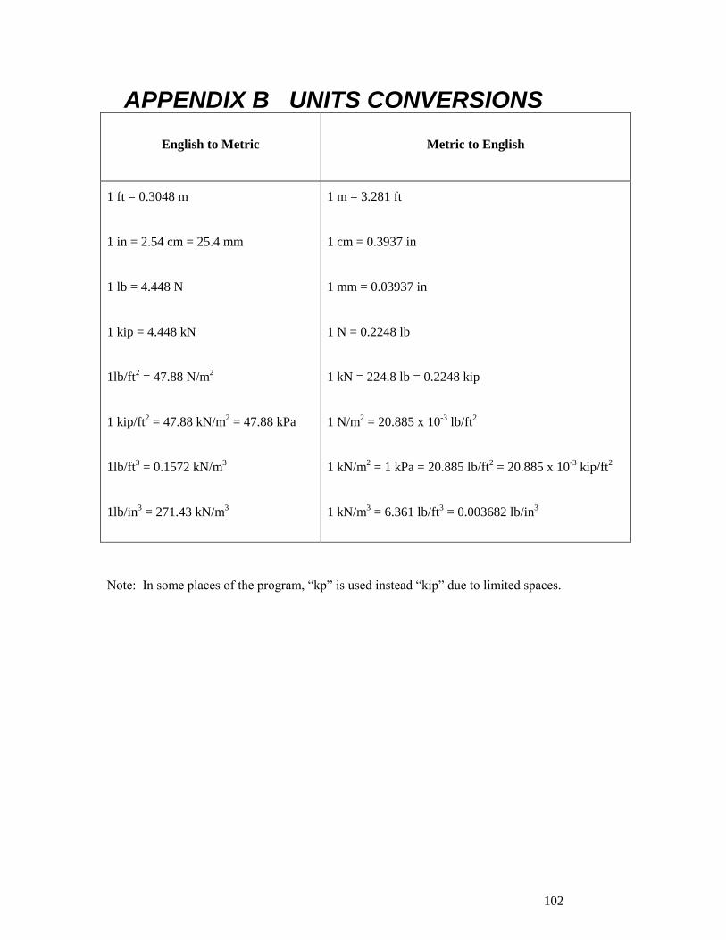
102
. . . . . . . . .
APPENDIX B UNITS CONVERSIONS
English to Metric
Metric to English
1 ft = 0.3048 m
1 in = 2.54 cm = 25.4 mm
1 lb = 4.448 N
1 kip = 4.448 kN
1lb/ft2 = 47.88 N/m
2
1 kip/ft2 = 47.88 kN/m
2 = 47.88 kPa
1lb/ft3 = 0.1572 kN/m
3
1lb/in3 = 271.43 kN/m
3
1 m = 3.281 ft
1 cm = 0.3937 in
1 mm = 0.03937 in
1 N = 0.2248 lb
1 kN = 224.8 lb = 0.2248 kip
1 N/m2 = 20.885 x 10
-3 lb/ft
2
1 kN/m2 = 1 kPa = 20.885 lb/ft
2 = 20.885 x 10
-3 kip/ft
2
1 kN/m3 = 6.361 lb/ft
3 = 0.003682 lb/in
3
Note: In some places of the program, “kp” is used instead “kip” due to limited spaces.


![[04899] - Design of Pile & Pile-Cap](https://static.fdocuments.net/doc/165x107/5695d3331a28ab9b029d273d/04899-design-of-pile-pile-cap.jpg)