Mangroves as a Source of Greenhouse Gases to theAtmosphere and Alkalinity and Dissolved Carbonto the Coastal Ocean: A Case Study From theEverglades National Park, FloridaGloria M. S. Reithmaier1 , David T. Ho2 , Scott G. Johnston1 , and Damien T. Maher1

1Southern Cross Geoscience, Southern Cross University, Lismore, New South Wales, Australia, 2Department ofOceanography, University of Hawaii at Manoa, Honolulu, HI, USA

Abstract Most research evaluating the potential of mangroves as a sink for atmospheric carbon hasfocused on carbon burial in sediments. However, the few studies that have quantified lateral exchange ofcarbon and alkalinity indicate that the dissolved carbon and alkalinity export may be several‐fold moreimportant than burial. This study aims to investigate rates and drivers of alkalinity, dissolved carbon, andgreenhouse gas fluxes of the mangrove‐dominated Shark River estuary located in the EvergladesNational Park in Florida, USA. Spatial surveys and 29‐hr time series were conducted to assess total alkalinity(TAlk), organic alkalinity (OAlk), dissolved inorganic carbon (DIC), dissolved organic carbon (DOC),carbon dioxide (CO2), methane (CH4), and nitrous oxide (N2O) dynamics. Dissolved carbon and greenhousegas concentrations were coupled to porewater input, which was examined using radon‐222. Shark Riverwas a source of CO2 (92 mmol/m2/day), CH4 (56 μmol/m2/day), and N2O (2 μmol/m2/day) to theatmosphere. Dissolved carbon export (DIC = 142 mmol/m2/day, DOC = 39 mmol/m2/day, normalized tomangrove area) was several‐fold higher than previously reported carbon burial rates in the study area(~28 mmol/m2/day). The majority of the DIC was exported as TAlk (97 mmol/m2/day), which remainsdissolved in the ocean for millennia and, therefore, represents a long‐term sink for atmospheric carbon. Byintegrating our results with previous studies, we argue that alkalinity, dissolved carbon, and greenhousegas fluxes should be considered in future blue carbon budgets.

Plain Language Summary Protecting mangroves can help us deal with one of the biggestchallenges of our time: Climate change. Mangroves remove carbon dioxide – the gas that is making theworld hotter – from the air around us and store it in their surrounding soils. Many scientists have studiedhow much carbon is trapped in mangrove soils, and the newest studies say that some of that trapped carbonis flushed out to the coastal ocean. We wanted to find out for ourselves so we went to Everglades NationalPark, which protects the biggest mangrove forest in North America. We cruised along the Shark Riverestuary and spent day and night on the boat to uncover this carbon mystery. We found that the estuary losesgreenhouse gasses to the atmosphere, but much less compared to what it loses to the Gulf of Mexico. Wecould also confirm that the amount of carbon lost was much greater than what is trapped in soils. Weencourage other researchers to investigate dissolved carbon export in other mangroves in order to find outhow much mangroves can alleviate the impacts of climate change.

1. Introduction

Mangroves play a disproportionately large role in the coastal carbon cycle, as carbon storage in these ecosys-tems is exceptionally high compared to other forest ecosystems (Donato et al., 2011). Globally, mangrovesoils store ∼2.6 Pg C (9.5 Pg of CO2) (Atwood et al., 2017), and the global carbon burial rate is estimatedto be ∼26 Tg C/y (Breithaupt et al., 2012). The blue carbon policy framework, which is increasingly usedto protect and restore coastal ecosystems, focuses on carbon burial of mangroves and other vegetated coastalhabitats. However, the carbon sink capacity of mangroves extends beyond carbon burial (Maher et al., 2018).Part of the buried carbon is remineralized and exported as dissolved carbon (Friesen et al., 2018; Maher,Santos, Golsby‐Smith, et al., 2013), which is largely unaccounted for in current blue carbon budgets.Furthermore, carbon remineralization results in greenhouse gas emissions, which partly offset carbon

©2020. American Geophysical Union.All Rights Reserved.

RESEARCH ARTICLE10.1029/2020JG005812

Key Points:• Two spatial surveys and two 29‐hr

time series were conducted toexplore the biogeochemistry of theShark River estuary

• The mangrove‐dominated estuarywas a source of dissolved carbon andgreenhouse gases

• Alkalinity, dissolved carbon andgreenhouse gas fluxes shouldbe integrated in future blue carbonbudgets

Correspondence to:G. M. S. Reithmaier,g.reithmaier.10@student.scu.edu.au

Citation:Reithmaier, G. M. S., Ho, D. T.,Johnston, S. G., & Maher, D. T. (2020).Mangroves as a source of greenhousegases to the atmosphere and alkalinityand dissolved carbon to the coastalocean: A case study from the EvergladesNational Park, Florida. Journal ofGeophysical Research: Biogeosciences,125, e2020JG005812. https://doi.org/10.1029/2020JG005812

Received 30 APR 2020Accepted 17 NOV 2020Accepted article online 28 NOV 2020

Author Contributions:Conceptualization: Gloria M. S.Reithmaier, David T. Ho, Damien T.MaherData curation: Gloria M. S.ReithmaierFormal analysis: Gloria M. S.Reithmaier, Damien T. MaherFunding acquisition: David T. Ho,Damien T. MaherInvestigation: Gloria M. S.Reithmaier, David T. Ho, Scott G.JohnstonMethodology: Gloria M. S.Reithmaier, David T. Ho, Damien T.MaherProject administration: David T. Ho,Damien T. MaherResources: David T. Ho, Damien T.MaherSupervision: Scott G. Johnston,Damien T. MaherVisualization: Gloria M. S. Reithmaier(continued)

REITHMAIER ET AL. 1 of 16

sequestration (Rosentreter et al., 2018b). To date, there are very few studies that examine and integrate allaspects of mangrove carbon cycling and their role in mitigating climate change, including carbon burial, car-bon remineralization, and subsequent lateral export, as well as greenhouse gas emissions.

Whether mangroves act as a source or sink for greenhouse gases appears to vary strongly between sites. Aportion of the carbon fixed by mangroves outgasses as CO2 to the atmosphere. The global average CO2 emis-sion by mangroves is estimated to be 34 ± 5 Tg C/y or 125 ± 18 Tg CO2/y (Rosentreter et al., 2018a), which isslightly higher than estimated global carbon burial rates in mangroves (26 Tg C/y; Breithaupt et al., 2012).Compared to CO2, total methane (CH4) emissions (water and sediment fluxes) by mangroves are thoughtto be small (0.2 ± 0.04 Tg C/y or 7.6 ± 1.5 Tg CO2 equivalents/y) (Rosentreter et al., 2018b). Nonetheless,accounting for CH4 emissions is important due to CH4 having a higher global warming potential, whichis defined as the amount of warming a gas causes over 100 y, when compared to CO2 (IPCC, 2014).Nitrous oxide (N2O), which is an even more potent greenhouse gas than CH4, is believed to be emitted atrates of 0.01–0.09 Tg N/y (4–37 Tg CO2 equivalents/y) by mangroves globally (Murray et al., 2015), but pris-tine mangroves can also act as N2O sink (Maher et al., 2016).

In addition to atmospheric exchanges, carbon is laterally exchanged between mangroves and the coastalocean. Dissolved carbon is predominantly exported to the coastal ocean as dissolved inorganic carbon(DIC = CO2 + HCO3

−+ CO32−) and to a lesser extent as dissolved organic carbon (DOC) (Faber et al., 2014;

Ho et al., 2017; Maher, Santos, Golsby‐Smith, et al., 2013; Taillardat et al., 2018). The global DOC exported bymangroves is estimated to be 24 ± 21 Tg C/y (Bouillon et al., 2008). Despite the important role of lateral DICexport, current global estimates (43 ± 12 Tg C/y) are derived from only six Australian mangrove creeks(Sippo et al., 2016). This limited spatial coverage of lateral DIC export estimates represents a significant bar-rier to developing a holistic understanding of global mangrove carbon cycling. During export to the coastalocean, DIC partly outgasses as CO2 to the atmosphere, whereas carbonate alkalinity (HCO3

−+ 2CO32−) can

effectively remain dissolved in the ocean with an oceanic residence time of ~100,000 y (Emerson &Hedges, 2008; Middelburg et al., 2020). Therefore, lateral export of total alkalinity (TAlk) can represent along‐term atmospheric carbon sink, which might be comparable to soil organic carbon stocks (Faberet al., 2014; Maher et al., 2018; Sippo et al., 2016).

An understudied component of TAlk is organic alkalinity (OAlk). Previous studies have found significantcontributions of OAlk in rivers (Hunt et al., 2011), estuaries (Cai et al., 1998; Tishchenko et al., 2006), coastalwaters (Hernández‐Ayon et al., 2007; Hunt et al., 2011; Ko et al., 2016), and the open ocean (Fong &Dickson, 2019). In the coastal and marine environment, OAlk is produced by photosynthesis, for instanceby phytoplankton (Kim& Lee, 2009) and algae (Hernández‐Ayon et al., 2007), or by carbon remineralization(Lukawska‐Matuszewska et al., 2018). To our knowledge, research investigating OAlk in mangroves islimited to one study, which reported OAlk values up to 47 μmol/kg for seven‐point measurements (Yanget al., 2015).

This study aims to update the mangrove carbon and greenhouse gas budget, with a specific focus on aquaticexports, by examining alkalinity, dissolved carbon, and greenhouse gas fluxes in the mangrove‐dominateShark River located in Everglades National Park, Florida, USA. We quantified estuarine fluxes and evalu-ated their underlying drivers, such as carbon remineralization and porewater inputs, by applying contrastingspatial surveys and time series approaches. Furthermore, we present the first study analyzing the dynamicsand relevance of OAlk in mangrove‐dominated estuaries.

2. Methods2.1. Study Site

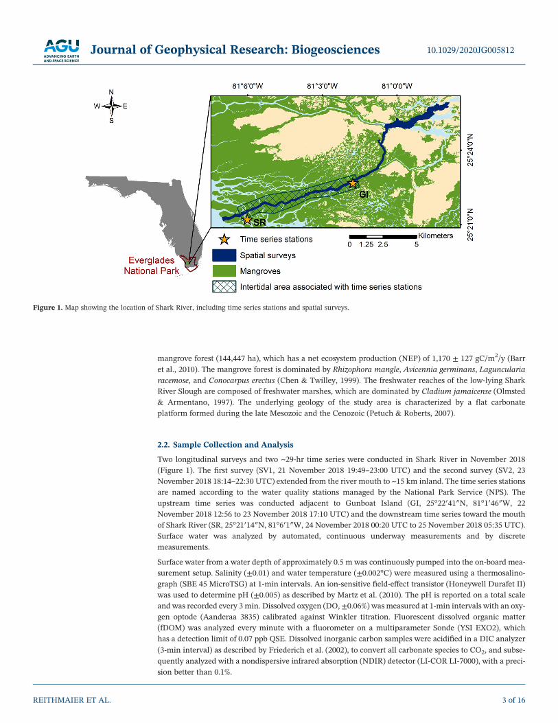
Shark River is located in Everglades National Park, South Florida, USA (Figure 1) and flows into the Gulf ofMexico. The subtropical climate of South Florida is characterized by a dry season from November to April(average monthly rainfall 54 mm) and a wet season from May to October (average monthly rainfall189 mm). Average monthly minimum and maximum temperatures range between 12°C and 34°C(Southeast Regional Climate Center; http://www.sercc.com). The area is subject to a semidiurnal tidalregime, with a mean tidal amplitude of 0.5–1 m. The estuary has an average depth of 2.8 m, a total intertidalarea of 15.9 km2 (Ho et al., 2014), and a surface area of 3.4 km2. Shark River is surrounded by a large

10.1029/2020JG005812Journal of Geophysical Research: Biogeosciences

REITHMAIER ET AL. 2 of 16

Writing – original draft: Gloria M. S.ReithmaierWriting – review & editing: David T.Ho, Scott G. Johnston, Damien T.Maher

mangrove forest (144,447 ha), which has a net ecosystem production (NEP) of 1,170 ± 127 gC/m2/y (Barret al., 2010). The mangrove forest is dominated by Rhizophora mangle, Avicennia germinans, Lagunculariaracemose, and Conocarpus erectus (Chen & Twilley, 1999). The freshwater reaches of the low‐lying SharkRiver Slough are composed of freshwater marshes, which are dominated by Cladium jamaicense (Olmsted& Armentano, 1997). The underlying geology of the study area is characterized by a flat carbonateplatform formed during the late Mesozoic and the Cenozoic (Petuch & Roberts, 2007).

2.2. Sample Collection and Analysis

Two longitudinal surveys and two ~29‐hr time series were conducted in Shark River in November 2018(Figure 1). The first survey (SV1, 21 November 2018 19:49–23:00 UTC) and the second survey (SV2, 23November 2018 18:14–22:30 UTC) extended from the river mouth to ~15 km inland. The time series stationsare named according to the water quality stations managed by the National Park Service (NPS). Theupstream time series was conducted adjacent to Gunboat Island (GI, 25°22′41″N, 81°1′46″W, 22November 2018 12:56 to 23 November 2018 17:10 UTC) and the downstream time series toward the mouthof Shark River (SR, 25°21′14″N, 81°6′1″W, 24 November 2018 00:20 UTC to 25 November 2018 05:35 UTC).Surface water was analyzed by automated, continuous underway measurements and by discretemeasurements.

Surface water from a water depth of approximately 0.5 m was continuously pumped into the on‐board mea-surement setup. Salinity (±0.01) and water temperature (±0.002°C) were measured using a thermosalino-graph (SBE 45 MicroTSG) at 1‐min intervals. An ion‐sensitive field‐effect transistor (Honeywell Durafet II)was used to determine pH (±0.005) as described by Martz et al. (2010). The pH is reported on a total scaleand was recorded every 3 min. Dissolved oxygen (DO, ±0.06%) was measured at 1‐min intervals with an oxy-gen optode (Aanderaa 3835) calibrated against Winkler titration. Fluorescent dissolved organic matter(fDOM) was analyzed every minute with a fluorometer on a multiparameter Sonde (YSI EXO2), whichhas a detection limit of 0.07 ppb QSE. Dissolved inorganic carbon samples were acidified in a DIC analyzer(3‐min interval) as described by Friederich et al. (2002), to convert all carbonate species to CO2, and subse-quently analyzed with a nondispersive infrared absorption (NDIR) detector (LI‐COR LI‐7000), with a preci-sion better than 0.1%.

Figure 1. Map showing the location of Shark River, including time series stations and spatial surveys.

10.1029/2020JG005812Journal of Geophysical Research: Biogeosciences

REITHMAIER ET AL. 3 of 16

Concentrations of CO2, N2O, CH4 (1‐min intervals), and radon‐222 (222Rn, 10‐min intervals) were measuredvia a showerhead equilibrator coupled to gas analyzers (Santos et al., 2012). Concentrations of CO2 and CH4

were analyzed during SV1 and time series at GI with a mobile gas concentration analyzer (PicarroGasScouter™ G4301) with a raw precision of 0.4 ppm and 3 ppb, respectively. N2O concentrations(±2 ppb) for the entire sampling period and CO2 (±10 ppm) and CH4 (±10 ppb) concentrations for SV2and the SR time series were analyzed by cavity ring‐down spectroscopy (Picarro G2308) (Maher, Santos,Leuven, et al., 2013). Methods of CO2 and CH4 measurements varied temporarily due to equipment failure.Methods with the largest data coverage have been selected for each survey or time series. Simultaneous mea-surements (31 hr) of both instruments showed that CO2 and CH4 measurements differed by less than 12%,justifying the use of both methods. A radon detector (Durridge RAD7) was used to measure 222Rn (Burnettet al., 2001). Equilibration times of all gases were corrected according to Webb et al. (2016), shifting the datasets by 30min for 222Rn and CH4 and by 10min for CO2 andN2O. This approachwas validated by comparingmeasured pCO2 and calculated pCO2 (using measured DIC and pH).

Discrete samples for TAlk, OAlk, and DOC were taken hourly during the time series and at salinity changesof approximately two salinity units during the spatial surveys. For TAlk and OAlk analysis, samples werefiltered with 0.7 μm GFF filters and measured within 1 day, using a titrator (Metrohm 888 Titrando withTiamo light), which has a precision better than 5 μM. Deviations and drifts in the acid concentration(0.05 M hydrochloric acid) were accounted for, using certified reference materials (CRM batch 175 andCRM batch 178) according to Dickson (2010). The method developed by Cai et al. (1998) was adapted forOAlk determination. Following the first Gran titration, which determines TAlk, samples were purged withultrahigh purity (99.999%) N2 for 5 min to remove the CO2 and then back‐titrated to the initial pH withsodium hydroxide (0.05 M). Subsequently, a second Gran titration was undertaken on the sample, whichdetermines the noncarbonate alkalinity. To calculate OAlk, results were corrected for borate alkalinity,which was calculated from DIC, pH, temperature, and salinity using CO2SYS Version 2.5 (Lewis &Wallace, 1998). Within CO2SYS, the dissociation constants of Millero (2010) were chosen, which apply toestuarine waters. For the remaining settings we used “KHSO” from Dickson (1990), “KHF” from Perezand Fraga (1987), and the “[B]T Value” from Lee et al. (2010). The calculated borate alkalinity ranged from0.3–47 μmol/kg and accounted for, on average, 17% of the noncarbonate alkalinity. For DOC analysis, sam-ples were filtered with 0.7 μmGFF filters, preserved with phosphoric acid, and analyzed with a total organiccarbon analyzer (Shimadzu TOC‐L CSH/CSN), which has a precision better than 2%.

2.3. Calculations2.3.1. Lateral Alkalinity and Dissolved Carbon FluxesA Lagrangian method has been applied to analyze lateral fluxes of alkalinity and dissolved carbon to deter-mine the exchange between the estuary and the coastal ocean as described by Ho et al. (2017). Briefly, theestuary was divided into 100‐m longitudinal sections. For each survey, DIC, TAlk, DOC, and OAlk concen-trations were corrected for tidal excursion using current speed at GI (U.S. Geological Survey, 2018).Polynomial functions were fitted to the measured concentrations as a function of salinity to increase the datadensity (allowing for a concentration value to be assigned to each salinity measurement). These data werethen used to calculate the moles of each constituent within each section by multiplying average concentra-tion within each section by the corresponding volume. The mass of constituent within each section wassummed across the entire study domain to calculate estuarine inventory. The polynomial fits were highlyrepresentative for DIC (SV1: R2 = 0.99, RMSE = 31 μmol/L, SV2: R2 = 0.99, RMSE = 44 μmol/L), TAlk(SV1: R2 = 0.99, RMSE = 53 μmol/L; SV2: R2 = 0.99, RMSE = 39 μmol/L), DOC (SV1: R2 = 0.98,RMSE = 42 μmol/L; SV2: R2 = 0.96, RMSE = 60 μmol/L), and OAlk (SV1: R2 = 0.99, RMSE = 31 μmol/L;SV2: R2 = 0.99, RMSE = 44 μmol/L). In order to calculate estuarine fluxes, the inventories have been cor-rected for conservative mixing. Conservative mixing lines were fitted by connecting observed values at thelowest and highest salinities.

Lateral fluxes were calculated, assuming the systemwas in steady state, by dividing the inventories correctedfor conservative mixing by the water residence time (8.3 days), which was calculated by applying an equationdeveloped for Shark River by Ho et al. (2016):

10.1029/2020JG005812Journal of Geophysical Research: Biogeosciences

REITHMAIER ET AL. 4 of 16

τ ¼ 3:678þ 26:718e−0:367Q (1)

where τ is the residence time and Q (4.8 m3/s) is the tidally filtered discharge at Gunboat Island, whichwas retrieved from U.S. Geological Survey (2018), who used the index‐velocity method for tidal filtering(Ruhl & Simpson, 2005). Assuming steady state during the measurement period is reasonable since theresidence time was short, and Volta et al. (2018) found that carbon fluxes varied by little within each sea-son at Shark River. Positive values represent lateral exports to the ocean. Rates were normalized to theassociated tidally inundated area (15.9 km2) for Shark River (Ho et al., 2017) for comparison with previousstudies. Due to the high uncertainty about this area, ranges for areal fluxes were determined by using halfand twice the size of the inundated area.

In addition to the Lagrangian approach, an Eulerian method was applied to quantify lateral fluxes. LateralTAlk, DIC, and DOC fluxes were calculated bymultiplying concentrations, which were sampled during timeseries measurements, with discharge at 15‐min intervals. To attain higher temporal resolution for TAlk,OAlk, and DOC flux rates, TAlk was calculated using CO2SYS from high‐resolution measurements ofDIC and pH (Pierrot et al., 2009), and DOC, as well as OAlk, was calculated from fDOM using linear rela-tionships (see section 3.3). Concentrations were averaged for each time step. Discharge values (15‐min inter-vals) were retrieved from the U.S. Geological Survey station at Gunboat Island and ranged from −186 to 189m3/s during the GI time series and from −239 to 218 m3/s during the SR time series, which negative valuesrepresenting fluxes in the upstream direction (U.S. Geological Survey, 2018). Start and end time wereadjusted to balance the water volumes and included two complete tidal cycles. The overall Eulerian lateralexport was calculated as the difference between the lateral fluxes at both time series stations, which can beattributed to the input by the mangrove‐dominated area in between. Positive values indicate fluxes directedtoward the ocean.

To get area‐normalized rates (i.e., mmol/m2/day), total fluxes have been scaled to the estimated inundatedarea between the time series stations (8.7 km2), which is shown in Figure 1. Due to the lack of ahigh‐resolution digital elevation model (DEM), the boundary of the intertidal area has been examinedmanually in ArcMap. The area is characterized by extremely flat terrain and a complex network of streams.During high tide, the areas between the streams are largely flooded, interconnecting the streams, making itcomplicated to assign an accurate drainage area to a single stream. Therefore, the boundary of the inundatedarea has been defined arbitrarily as halfway between Shark River and the largest neighboring streams,assuming that 50% of the inundated water drains to Shark River and 50% to the largest neighboring streams.To account for this large uncertainty, uncertainty bands for the areal fluxes have been examined by halvingand doubling the inundation area.2.3.2. Greenhouse Gas FluxesConcentrations of CO2, CH4, and N2O were corrected for water vapor removal and converted to partial pres-sure according to the methods detailed in Pierrot et al. (2009). Air‐water gas fluxes of O2, CO2, CH4, and N2Owere determined (1‐min intervals), as a product of the gas transfer velocity, the solubility coefficient, and thedifference in the air‐water partial pressure:

FGas ¼ kGas K0 pGas waterð Þ–pGas airð Þ� �

(2)

where FGas is the gas flux (mmol/m2/day), kGas is the gas transfer velocity, K0 is the solubility coefficient,pGas(water) is the partial gas pressure in water, and pGas(air) is the partial gas pressure in the air. The solu-bility coefficients were calculated as a function of salinity and temperature for O2 (Benson &Krause, 1984), CO2 (Weiss, 1974), CH4 (Wiesenburg & Guinasso, 1979), and N2O (Weiss & Price, 1980).Atmospheric partial pressures of 412 μatm for CO2, 1.8 μatm for CH4, and 0.33 μatm for N2O were used(European Environment Agency, 2019). According to the convention, positive values represent a fluxtoward the atmosphere. The gas transfer velocity was calculated:

kGas ¼ k 600ð Þ ScGas=600ð Þ−0:5; (3)

where k(600) is the gas transfer velocity normalized to a Schmidt number of 600 and ScGas is theSchmidt number, which was calculated as a function of temperature and salinity assuming a linear

10.1029/2020JG005812Journal of Geophysical Research: Biogeosciences

REITHMAIER ET AL. 5 of 16

dependence of the Schmidt number on salinity (Wanninkhof, 2014). We integrated wind speed, currentvelocity, and water depth to calculate k(600) according to Ho et al. (2016), who conducted 3He/SF6deliberate gas tracer experiments in the Shark River to derive an empirical equation for k(600)determination:

k 600ð Þ ¼ 0:77v0:5 h−0:5 þ 0:266u102; (4)

where v is the current velocity, h is the mean depth of Shark River (2.8 m) (Ho et al., 2014), and u10 is thewind speed at 10 m height, which was recorded on‐site (0.81 and 1.88 m/s) with a sonic anemometer(ATMOS 41). Gas fluxes were interpolated to the water area of the entire Shark River estuary (2.2 km2)and the area between the time series stations (0.9 km2)—see Figure 1—using the spatial analyst tool“spine,” which uses a series of linear equations to minimize curvature of the interpolated surface(Franke, 1982), followed by masking the interpolated file with the shape of Shark River in ArcGIS10.6.1 (Maher & Eyre, 2012).2.3.3. Statistical AnalysisStatistical analysis was conducted in SigmaPlot 14.0. The Pearson correlation coefficients (r) were deter-mined for alkalinity, dissolved carbon, greenhouse gases, and the explanatory variables (salinity, 222Rn,and DO) to evaluate underlying drivers. The probability levels are presented as *if p < 0.05, **if p < 0.01,and ***if p < 0.001. Testing the use of potential proxies, linear regressions between OAlk, DOC, and fDOMhave been determined, reporting coefficients of determination (R2).

3. Results3.1. Spatial Surveys

Ranges and trends of all measured parameters varied little between the two spatial surveys (Figure 2). DOsaturation (36–82%) and pH (7.4–7.8) showed a concave down pattern along the salinity gradient, whichranged from 0.7 to 29. The average water temperature during SV1 (25.9°C) was slightly higher than duringSV2 (25.2°C). 222Rn decreased toward the river mouth (3,173–5,246 dpm/m3). During both surveys, pCO2

(1,299–5,872 μatm) increased at intermediate salinities. In contrast, CH4 (18–109 μatm) and N2O(0.36–0.47μatm) decreased toward higher salinity. Both TAlk and DIC showed similar concentrations andtrends ranging from 2,913 to 4,255 μmol/kg and from 2,753 to 4,277 μmol/kg, respectively. Concentrationsof OAlk (0–81 μmol/kg), DOC (604–1,422 μmol/L), and fDOM (39–161 ppb) decreased with increasingsalinity. The overall trends along the salinity gradient during the spatial surveys were similar to the trendsobserved during the time series. Due to equipment failure, no 222Rn and pCH4 data exist for SV2.

3.2. Time Series

The two time series stations were exposed to contrasting salinity ranges, with values ranging from 3 to 22 atGI and from 26 to 29 at SR (Figure 3). The upstream site GI experienced freshwater DO input during low tideand seawater DO input during high tide (34–41% saturation), and the pH ranged between 7.4 and 7.6. Thedownstream site SR was mainly influenced by the ocean, and DO (34–84% saturation) and pH (7.6–7.9) werepositively correlated with salinity. Water temperatures were similar at both time series stations, averaging24.8°C. At the GI site, 222Rn reached twofold higher values (5,648–9,969 dpm/m3) compared to the SR site(3,473–6,515 dpm/m3).

At both stations, CO2, CH4, N2O, TAlk, DIC, DOC, and fDOM were higher during low tides (lower salinity)than during high tides (Figure 3). During the time series at GI, pCO2 (3,976–6,239 μatm) and pCH4 (47–100μatm) were several‐fold higher compared to pCO2 (1,256–2,272 μatm) and pCH4 (12–34 μatm) at SR. Incontrast, N2O reached almost similar values at both stations (0.35–0.42 μatm). At GI, TAlk ranged from3,704–4,368 μmol/kg and at SR from 2,832–3,315 μmol/kg. Concentrations of DIC ranged from3,702–4,348 μmol/kg at GI and from 2,765–3,214 μmol/kg at SR. Due to equipment failure, OAlk data areonly available for the GI site (35–61 μmol/kg). Concentrations of DOC were two times and fDOM was threetimes higher at GI (934–1,458 μmol/L, 91–159 ppb) compared to SR (504–825 μmol/L, 35–59 ppb).

10.1029/2020JG005812Journal of Geophysical Research: Biogeosciences

REITHMAIER ET AL. 6 of 16

3.3. Drivers of Alkalinity, Dissolved Carbon, and Greenhouse Gas Dynamics

Pearson's correlation coefficients between alkalinity, dissolved carbon, greenhouse gases, and the explana-tory variables salinity, DO, and 222Rn provide insights into underlying drivers of estuarine processes(Table 1). Salinity was a good predictor (negatively correlated) for all parameters during all measurements.DO (a proxy for aerobic metabolism) was also negatively correlated to most parameters, with the exceptionof N2O during the GI time series. The natural groundwater tracer 222Rn was positively correlated to all para-meters except OAlk (all experiments) and DOC at SR.

We explored potential proxies for OAlk and DOC (Figure 4). Linear regressions showed that DOC (R2 = 0.78)and fDOM (R2 = 0.78) were good predictors for OAlk. Furthermore, fDOM was an excellent proxy for DOC(R2 = 0.98) over a broad salinity range. The high correlation between fDOM and DOC indicates that mea-surements with fDOM sensors are a cost and time efficient substitution for high‐resolution OAlk andDOC monitoring in Shark River and potentially other mangrove dominated systems.

Figure 2. Biochemical parameters were measured during two spatial surveys along the Shark River. Salinity gradients of (a) oxygen (DO), (b) radon‐222 (222Rn),(c) temperature, (d) carbon dioxide (pCO2), (e) methane (pCH4), (f) nitrous oxide (pN2O), (g) total alkalinity (TAlk), (h) dissolved inorganic carbon (DIC), (i) pH,(j) organic alkalinity (OAlk), (k) dissolved organic carbon (DOC) and (l) fluorescent dissolved organic matter (fDOM). The pH is shown on a total scale.Dashed lines represent conservative mixing lines.

10.1029/2020JG005812Journal of Geophysical Research: Biogeosciences

REITHMAIER ET AL. 7 of 16

Figure 3. Biochemical parameters were measured at upstream (GI) and downstream (SR) time series stations at Shark River. Salinity gradients of (a) oxygen(DO), (b) radon‐222 (222Rn), (c) temperature, (d) carbon dioxide (pCO2), (e) methane (pCH4), (f ) nitrous oxide (pN2O), (g) total alkalinity (TAlk), (h)dissolved inorganic carbon (DIC), (i) pH, ( j) organic alkalinity (OAlk), (k) dissolved organic carbon (DOC) and (l) fluorescent dissolved organic matter (fDOM).The pH is shown on a total scale. Arrows pointing right indicate flood and arrows pointing left indicate ebb tides.

Table 1Pearson Correlations Between Dissolved Carbon, Alkalinity, Greenhouse Gases, and the Explanatory Variables for Upstream (GI) and Downstream (SR) Time Seriesand Both Spatial Surveys (SV)

Variable DIC TAlk DOC OAlk CO2 CH4 N2O

SV Salinity −0.73*** −0.7*** −0.96*** −0.92*** −0.83*** −0.89*** −0.82***

DO −0.9*** −0.84*** −0.5* −0.3 −0.9*** −0.17* −0.51***222Rn 0.84*** 0.65* 0.66* 0.03 0.74*** 0.83*** 0.85***

SR Salinity −0.96*** −0.74*** −0.48* NA −0.91*** −0.86*** −0.73***

DO −0.61*** −0.32 −0.32 NA −0.67*** −0.77*** −0.49***222Rn 0.72*** 0.64*** 0.26 NA 0.75*** 0.79*** 0.61***

GI Salinity −0.89*** −0.86*** −0.94*** −0.78*** −0.95*** −0.8*** −0.43***

DO −0.64*** −0.49* −0.36 −0.14 −0.67*** −0.12*** 0.16***222Rn 0.33*** 0.42* 0.57** 0.36 0.45*** 0.76*** 0.56***

Note. Due to equipment failure, no OAlk data are available for the SR time series. The probability levels are presented as* if p < 0.05,** if p < 0.01 and*** if p < 0 .001.

10.1029/2020JG005812Journal of Geophysical Research: Biogeosciences

REITHMAIER ET AL. 8 of 16

3.4. Alkalinity, Dissolved Carbon, and Greenhouse Gas Fluxes

Shark River was a source of all measured greenhouse gases to theatmosphere and a sink for DO (Table 2). Referenced to the water areabetween the time series stations (0.94 km2), DO uptake by the river(−2.1 × 105 mol/day) was threefold higher than CO2 emissions(6.4 × 104 mol/day). In comparison, CH4 emissions (28 mol/day) playedonly a minor role, and N2O emissions (1 mol/day) were negligible.

During the time series measurements, dissolved carbon and alkalinitywere exported to the ocean (Table 2). The lateral fluxes at GI (upstream)were considerably lower, constituting only 4–15% of the lateral fluxes atSR (downstream). At GI, DIC and DOC fluxes were comparable, whereasat SR, DIC was the major dissolved carbon export (76% of the total).Lateral fluxes of DIC and TAlk were similar (1 × 106 mol/day) at SR, butat GI, DIC (5 × 104 mol/day) was lower than TAlk (1 × 105 mol/day).At both sites, the OAlk flux accounted for 2% of the TAlk flux and 5% ofthe DOC flux. Lateral fluxes estimated with the Lagrangian approach,which calculated fluxes of the entire estuary, were slightly lower thanthe fluxes determined using the Eulerianmethod (Table 2), which focusedon the mangrove‐dominated section of the estuary.

4. Discussion4.1. Drivers of Alkalinity, Dissolved Carbon, and GreenhouseGas Dynamics

Despite the comprehensive data acquisition during the measurementspresented here, our measurements were conducted over a short period.Alkalinity, dissolved carbon, and greenhouse gases are known to varybetween seasons (Koné & Borges, 2008; Volta et al., 2018) and over springneap cycles (Call et al., 2015) within mangrove systems. Therefore, whileour data provide insights into the flux rates and mechanisms driving car-bon and greenhouse gas dynamics in Shark River during the study period,long‐term seasonal and interannual variability cannot be assessed.

In estuarine sediments, TAlk, dissolved carbon, and greenhouse gases areknown to be driven by redox reactions coupled to remineralization oforganic matter (Burdige, 2011). The relative importance of different meta-bolic processes as well as carbonate dissolution can be examined throughlinear regression of salinity normalized TAlk (TAlkn) and salinity normal-ized DIC (DICn) (Bouillon et al., 2007; Friis et al., 2003). The TAlkn:DICn

ratios are characteristic for the prevailing process:−0.2 for aerobic respira-tion, 0.8 for denitrification, 1.0 for sulfate reduction, 2.0 for CaCO3 disso-lution, 4.0 for manganese reduction, and 8.0 for iron reduction.

The TAlkn:DICn ratios found during the spatial surveys (0.87), and the GI (0.64) and SR (0.45) time series(Figure 5) are within the range of ratios reported in the literature (0.44–0.92), which have been interpretedas a mixture of sulfate reduction and aerobic respiration, which are commonly the dominant estuarine remi-neralization processes (Bouillon et al., 2007; Ho et al., 2017; Koné & Borges, 2008; Sippo et al., 2016; Zablockiet al., 2011). The ratio of individual time series and the surveys varied considerably, suggesting spatial andtemporal changes of the dominant metabolic processes. The overall ratio (0.93), combing all measurements,was slightly higher than previously reported values, which might be due to the additional TAlk productionfrom carbonate dissolution since Shark River drains a large carbonate basin. Similarly, Ho et al. (2017) foundhigh TAlkn:DICn ratios (0.84–0.92) during earlier surveys at Shark River.

In addition to carbonate alkalinity, OAlk can contribute to TAlk within carbon‐rich systems. At Shark River,OAlk concentrations (0–81 μmol/kg) accounted for ~1% of TAlk, and the concentrations were comparable to

Figure 4. Correlations between organic alkalinity (OAlk) and (a) dissolvedorganic carbon (DOC) and (b) fluorescent dissolved organic matter (fDOM).fDOM was highly correlated with DOC for both the surveys and timeseries (c). Linear regression lines are presented for the individual time series(GI and SR) and spatial surveys (SV). All linear regressions had probabilitylevels of p < 0.001, except for fDOM versus DOC at SR (p = 0.004).

10.1029/2020JG005812Journal of Geophysical Research: Biogeosciences

REITHMAIER ET AL. 9 of 16

literature values for mangroves and other vegetated coastal habitats. Yang et al. (2015) calculated OAlk forseven mangrove sites in the Gulf of Mexico, Florida, reporting values up to 47 μmol/kg for salinities higherthan 23. Measuring OAlk along salinity gradients of saltmarsh dominated rivers in Georgia, Cai et al. (1998)found OAlk concentrations ranging from 8 to 112 μmol/L. At a Ramsar site in San Quintín Bay, Mexico,which is vegetated by seagrasses and saltmarshes, OAlk concentrations ranged between 20 and 75 μmol/kg (Hernández‐Ayon et al., 2007). The small share of OAlk concentrations to TAlk concentrations (on aver-age 1% for all measurements) compared to previous studies (up to 23%) (Cai et al., 1998) is attributed to thehigher overall TAlk concentrations (up to 4,368 μmol/kg) in Shark River.

Within estuaries, sediments are often a dominant source of TAlk, dissolved carbon, and greenhouse gases.These metabolic products can be delivered to surface waters via porewater exchange, which inmangrove‐dominated systems is primarily driven by tidal pumping (Call et al., 2015; Chen et al., 2018;Maher, Santos, Golsby‐Smith, et al., 2013). Positive correlations between TAlk, dissolved carbon, and green-

house gases with 222Rn (Table 1) suggest that porewater input might be animportant driver of carbon cycling at Shark River. Similarly, previous stu-dies reported positive correlations for 222Rn with TAlk, DIC, DOC, CO2,CH4, and N2O in mangroves (Call et al., 2015, 2019; Faber et al., 2014;Maher, Santos, Golsby‐Smith, et al., 2013; Reading et al., 2017;Sadat‐Noori et al., 2016; Taillardat et al., 2018). Maher, Santos, Golsby‐Smith, et al. (2013) found that 89–92% of DOC and 93–99% of DIC exportfrom a subtropical mangrove creek were driven by porewater input.Results of Call et al. (2015) showed that porewater exchange controlledCO2 and CH4 concentrations with exchange rates driven by tidal ampli-tude changes over spring‐neap cycles. Santos et al. (2019) reported signif-icant porewater fluxes of TAlk (124 ± 131 mmol/m2/day), DIC(256 ± 203 mmol/m2/day), DOC (283 ± 190 mmol/m2/day), CO2

(120 ± 78 mmol/m2/day), and CH4 (1.2 ± 0.8 mmol/m2/day) at a subtro-pical mangrove and saltmarsh dominated creek.

4.2. Alkalinity, Dissolved Carbon, and Greenhouse Gas Fluxes

The investigation of seasonal changes was beyond the scope of this study,since our measurements have been limited to a short period. However,

Table 2Air‐Water Greenhouse Gas Fluxes and Lateral Fluxes of Alkalinity and Dissolved Carbon

Air‐water DO flux CO2 flux CH4 flux N2O flux

Shark River (mol/day) −6.3 × 105 2.0 × 105 123 3.6Shark River (mmol/m2/day) −285 92 0.06 0.002Mangrove area (mol/day) −2.1 × 105 6.4 × 104 28 1.0Mangrove area (mmol/m2/day) −222 68 0.03 0.001

Lateral DIC flux TAlk flux DOC flux OAlk flux

GI station (mol/day) 5.5 × 104 1.3 × 105 5.5 × 104 2.9 × 103

SR station (mol/day) 1.3 × 106 9.7 × 105 4.0 × 105 2.0 × 104

Eulerian (mol/day) 1.2 × 106 8.4 × 105 3.4 × 105 1.7 × 104

Eulerian (mmol/m2/day) 142 (71–284) 97 (48–193) 39 (20–79) 1.9 (1.0–3.9)Lagrangian (mol/day) 3.3 × 105 2.5 × 105 4.2 × 104 3.0 × 103

Lagrangian (mmol/m2/day) 21 (10–41) 16 (8–31) 3 (1–5) 0.2 (0.1–0.4)

Note. Air‐Water Gas Fluxes Are Shown for the Entire Surface Area of Shark River (3.4 km2) and the Mangrove‐Dominated Section of Shark River Between Time Series Stations (1.8 km2). Positive gas fluxes indicate fluxes towardthe atmosphere. Lateral fluxes are presented for the upstream station (GI), the downstream station (SR), and the inputby the tidally inundated mangrove‐dominated area (8.7 km2) between the time series stations using the Eulerianmethod. Lateral fluxes determined using the Lagrangian method have been scaled to the tidally indurated area ofthe entire estuary (15.9 km2) as proposed by Ho et al. (2017). Positive lateral fluxes indicate an export toward the coastalocean. Uncertainty bands for area‐normalized rates are shown in brackets.

Figure 5. Salinity normalised alkalinity (TAlkn) plotted against salinitynormalised dissolved inorganic carbon (DICn) for upstream (GI) anddownstream (SR) time series measurements and both spatial surveys (SV).

10.1029/2020JG005812Journal of Geophysical Research: Biogeosciences

REITHMAIER ET AL. 10 of 16

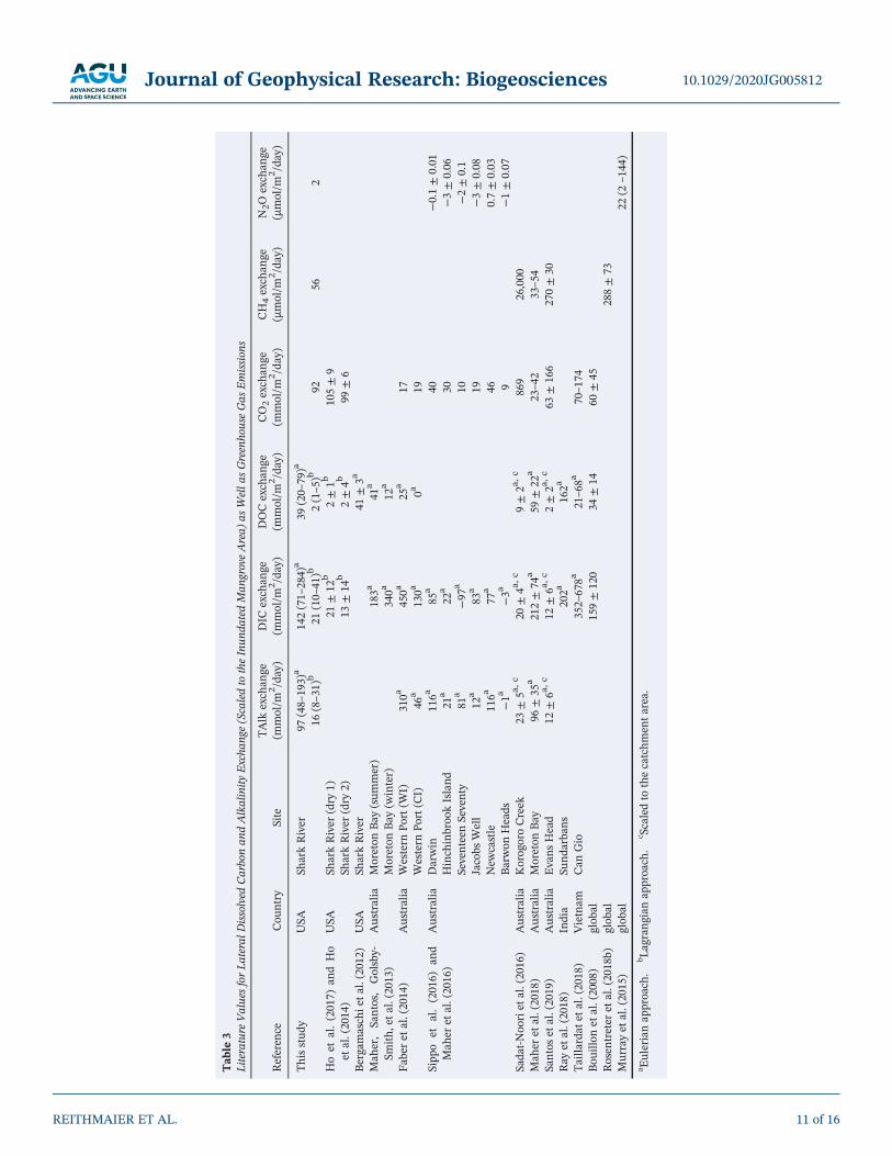
Tab

le3

LiteratureValuesforLateral

Dissolved

Carbonan

dAlkalinityExcha

nge

(Scaledto

theInun

datedMan

groveArea)

asWella

sGreenho

useGas

Emission

s

Referen

ceCou

ntry

Site

TAlk

exch

ange

(mmol/m

2 /da

y)DIC

exch

ange

(mmol/m

2 /da

y)DOCexch

ange

(mmol/m

2 /da

y)CO2exch

ange

(mmol/m

2 /da

y)CH4exch

ange

(μmol/m

2 /da

y)N2O

exch

ange

(μmol/m

2 /da

y)

Thisstud

yUSA

SharkRiver

97(48–193)a

142(71–284)a

39(20–79)a

16(8–31)b

21(10–41)b

2(1–5)b

9256

2Hoet

al.(2017)

andHo

etal.(2014)

USA

SharkRiver

(dry

1)21

±12

b2±1b

105±9

SharkRiver

(dry

2)13

±14

b2±4b

99±6

Bergamasch

ietal.(2012)

USA

SharkRiver

41±3a

Mah

er,

Santos,

Golsby‐

Smith,etal.(2013)

Australia

Moreton

Bay

(sum

mer)

183a

41a

Moreton

Bay

(winter)

340a

12a

Faber

etal.(2014)

Australia

Western

Port(W

I)310a

450a

25a

17Western

Port(CI)

46a

130a

0a19

Sipp

oet

al.(2016)

and

Mah

eret

al.(2016)

Australia

Darwin

116a

85a

40−0.1±0.01

Hinch

inbroo

kIsland

21a

22a

30−3±0.06

Seventeen

Seventy

81a

−97

a10

−2±0.1

Jacobs

Well

12a

83a

19−3±0.08

New

castle

116a

77a

460.7±0.03

Barwon

Heads

−1a

−3a

9−1±0.07

Sada

t‐Noo

riet

al.(2016)

Australia

KorogoroCreek

23±5a

,c

20±4a

,c

9±2a

,c

869

26,000

Mah

eret

al.(2018)

Australia

Moreton

Bay

96±35

a212±74

a59

±22

a23–42

33–54

Santoset

al.(2019)

Australia

EvansHead

12±6a

,c

12±6a

,c

2±2a

,c

63±166

270±30

Ray

etal.(2018)

India

Sunda

rban

s202a

162a

Tailla

rdat

etal.(2018)

Vietnam

Can

Gio

352–678a

21–68a

70–174

Bou

illon

etal.(2008)

glob

al159±120

34±14

60±45

Rosen

treter

etal.(2018b)

glob

al288±73

Murrayet

al.(2015)

glob

al22

(2–144)

a Eulerianap

proach

.bLagrangian

approach

.c Scaledto

thecatchmen

tarea.

10.1029/2020JG005812Journal of Geophysical Research: Biogeosciences

REITHMAIER ET AL. 11 of 16

analyzing fluxes at Gunboat Island (GI) for an entire year, Volta et al. (2018) found that DIC (23.2–25.4× 105 mol/day) and CO2 emissions (5.5–7.8 × 105 mol/day) varied little between seasons. Thus, eventhough this study was limited to a short period, the fluxes might still be representative of this site. AtShark River, TAlk, DIC, and DOC were produced within the estuary and exported to the Gulf of Mexico(Table 2). The lateral carbon export was dominated by DIC (87–89%), whereas DOC played only a minor role(11–13%). Similarly, previous studies showed that in mangroves most of the dissolved carbon is exported inthe form of DIC (Faber et al., 2014; Ho et al., 2017; Maher, Santos, Golsby‐Smith, et al., 2013; Maheret al., 2018; Taillardat et al., 2018).

To compare lateral export with literature values, fluxes were normalized to the tidally inundated area, whichwas associated with large uncertainties, resulting in large uncertainty ranges for the area‐normalized fluxes(Table 3). However, lateral TAlk, DIC and DOC fluxes were consistent with previously published rates forShark River as well as concordant with exchange rates reported for other mangrove‐dominated systems.The estuarine DIC and DOC fluxes, which have been calculated using the Lagrangian method, were nearlyidentical to earlier measurements at Shark River that were based on the same method (Ho et al., 2017).Compared to the Eulerian fluxes, the Lagrangian fluxes were considerably smaller, since the Lagrangianmethod covered the entire estuary with decreasing mangrove coverage in the upstream sections of the estu-ary (Figure 1). Further, the upper estuarine sections likely had lower rates of porewater exchange due to tidaldamping. In contrast, The Eulerian method covered a different study domain focusing on the mangrovedominated area in the lower estuary; therefore, higher area‐normalized rates highlight the influence of man-groves on estuarine carbon fluxes. Similarly, previous studies identified mangroves as major estuarinesources for dissolved carbon (Bouillon et al., 2007; Ray et al., 2018).

The majority of studies examining the lateral alkalinity and dissolved carbon exchange in mangroves usedthe Eulerian method, reporting rates concordant to our Eulerian exchange rates (Table 3). The TAlk export(48–193 mmol/m2/day) was within the range of previously reported TAlk exchange rates (−1–310 mmol/m2/day) of mangrove‐dominated sites. The DIC export (71–284 mmol/m2/day) was also in line with mea-sured literature rates (−97–678 mmol/m2/day) as well as the global DIC export (158 mmol/m2/day)estimated by Bouillon et al. (2008), who suggested that DIC fluxes may be the unaccounted carbon sink inmangroves. The Eulerian DOC export (20–79 mmol/m2/day) was similar to exchange rates reported by

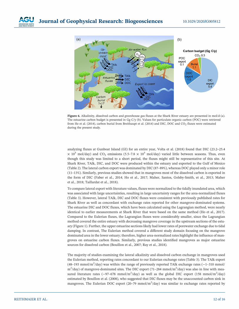
Figure 6. Alkalinity, dissolved carbon and greenhouse gas fluxes at the Shark River estuary are presented in mol/d (a).The estuarine carbon budget is presented in Gg C/y (b). Values for particulate organic carbon (POC) were retrievedfrom He et al. (2014), carbon burial from Breithaupt et al. (2014) and DIC, DOC and CO2 fluxes were estimatedduring the present study.

10.1029/2020JG005812Journal of Geophysical Research: Biogeosciences

REITHMAIER ET AL. 12 of 16

Bergamaschi et al. (2012) (41 mmol/m2/day) and consistent with the global average (34 mmol/m2/day)(Bouillon et al., 2008).

Shark River was a source of CO2, CH4, and N2O to the atmosphere. The air‐water flux of CO2

(92 mmol/m2/day) was close to previously measured emissions at this site (Ho et al., 2017) and was higherthan the global average for mangrove systems (60 mmol/m2/day) (Bouillon et al., 2008). High CO2 emissionsat Shark River are driven by upstream DIC input originating from freshwater marshes (Ho et al., 2017). Incontrast to CO2, CH4 (56 μmol/m2/day) and N2O emissions (2 μmol/m2/day) were much lower than theglobal average for mangroves (Murray et al., 2015; Rosentreter et al., 2018b). Air‐water fluxes of CH4 werepossibly reduced by increased CH4 oxidation within the water column as a result of oxygen‐rich fresh andsaltwater input, compared to more oxygen‐limited waters such as tidal creeks, which have been overrepre-sented in previous studies. Low N2O emissions might be due to nitrate limitation within the mangrove area(Inglett et al., 2011). Other pristine mangrove systems, which are naturally low in nitrogen, were found tohave minimal N2O emissions (Reading et al., 2017) and even N2O undersaturation (Maher et al., 2016).

The Shark River estuary was a net source of TAlk and dissolved carbon to the coastal ocean and a source ofgreenhouse gases to the atmosphere (Figure 6a). Alkalinity, dissolved carbon, and greenhouse gas fluxes atthe Shark River estuary are presented inmol/day (Figure 6a). The estuarine carbon budget is presented in GgC/y (Figure 6b). Values for particulate organic carbon (POC) were retrieved from He et al. (2014), carbonburial from Breithaupt et al. (2014), and DIC, DOC, and CO2 fluxes were estimated during the present study(Figure 6a). Most of the inorganic carbon was exported laterally (62–95%), whereas only a small share wasemitted to the atmosphere as CO2 and CH4. To provide an estimate of the complete carbon budget for theShark River estuary (Figure 6b), literature values have been used for lateral POC fluxes (He et al., 2014)and carbon burial rates (Breithaupt et al., 2014). It is important to note that these fluxes in this carbon budgethave been measured at different times and encompass different temporal scales. Nonetheless, the estimatedcarbon budget suggests that DIC export might be the dominant carbon flux at the Shark River estuary. TheEulerian DIC export (226–903 g C/m2/y) presented here was two to seven times higher than carbon burialrates (123 ± 19 g C/m2/y) of the mangrove forest surrounding Shark River estimated by Breithauptet al. (2014), thereby emphasizing the importance of considering lateral carbon export in blue carbonbudgets.

Averaging previously reported TAlk and DIC export rates and those determined during this study (Table 3)per latitudinal band and scaling it to the corresponding mangrove area to the global mangrove area (Giriet al., 2011) suggest a global TAlk export of 4.8 Tmol/y and a DIC export of 151 Tg C/y, which is an orderof magnitude higher than the global burial rate of ∼26 Tg C/y determined by Breithaupt et al. (2012).Both estimated export rates are higher than previous global estimates for TAlk (4.2 Tmol/y) and DIC(43 ± 12 Tg C/y) export, which were limited to six Australian mangrove creeks (Sippo et al., 2016).However, the global estimates presented here are based on a relatively small number of studies, and moreresearch is required to improve estimates of global TAlk and DIC export rates. This is especially the casein the low latitude tropics (0–5°) where most mangroves occur, yet the number of estimates of TAlk andDIC export rates remains very limited.

5. Conclusion

By combining spatial surveys and short‐term time series at the mangrove‐dominated Shark River, we foundthat the estuary was a source for alkalinity and dissolved carbon to the Gulf of Mexico and a source of green-house gases to the atmosphere. Carbonate dissolution and porewater inputs were identified as important dri-vers controlling carbon fluxes. Lateral TAlk export exceeds mangrove sedimentary carbon burial rates by atleast twofold, resulting in an underestimation of the net carbon sequestration effect of mangroves. The cli-mate change mitigation provided by the mangrove‐dominated estuary was partly offset by CH4 and N2Oemissions. However, greenhouse gas emissions were minor compared to carbon sequestration and alkalinityexport. We argue that accounting for lateral alkalinity and dissolved carbon export, as well as greenhouse gasfluxes, is crucial to more holistically evaluate the potential of mangroves to act as atmospheric carbon sinks.We, therefore, urge the scientific community to work toward integrating these processes into blue carbonbudgets.

10.1029/2020JG005812Journal of Geophysical Research: Biogeosciences

REITHMAIER ET AL. 13 of 16

Conflict of Interest

The authors declare that there is no conflict of interest.

Data Availability Statement

Data sets for this research are available on the PANGAEA database (https://doi.pangaea.de/10.1594/PANGAEA.916154).

ReferencesAtwood, T. B., Connolly, R. M., Almahasheer, H., Carnell, P. E., Duarte, C. M., Lewis, C. J. E., et al. (2017). Global patterns in mangrove soil

carbon stocks and losses. Nature Climate Change, 7(7), 523–528. https://doi.org/10.1038/NCLIMATE3326Barr, J. G., Engel, V., Fuentes, J. D., Zieman, J. C., O'Halloran, T. L., Smith, T. J. III, & Anderson, G. H. (2010). Controls on mangrove

forest‐atmosphere carbon dioxide exchanges in western Everglades National Park. Journal of Geophysical Research, 115, G02020.https://doi.org/10.1029/2009JG001186

Benson, B. B., & Krause, D. (1984). The concentration and isssotopic fractionation of oxygen dissolved in freshwater and seawater inequilibrium with the atmosphere. Limnology and Oceanography, 29(3), 620–632. https://doi.org/10.4319/lo.1984.29.3.0620

Bergamaschi, B. A., Krabbenhoft, D. P., Aiken, G. R., Patino, E., Rumbold, D. G., & Orem, W. H. (2012). Tidally driven export of dissolvedorganic carbon, total mercury, and methylmercury from a mangrove‐dominated estuary. Environmental Science & Technology, 46(3),1371–1378. https://doi.org/10.1021/es2029137

Bouillon, S., Borges, A. V., Castañeda‐Moya, E., Diele, K., Dittmar, T., Duke, N. C., et al. (2008). Mangrove production and carbon sinks: Arevision of global budget estimates. Global Biogeochemical Cycles, 22, GB2013. https://doi.org/10.1029/2007GB003052

Bouillon, S., Dehairs, F., Velimirov, B., Abril, G., & Borges, A. V. (2007). Dynamics of organic and inorganic carbon across contiguousmangrove and seagrass systems (Gazi Bay, Kenya). Journal of Geophysical Research, 112, G02018. https://doi.org/10.1029/2006JG000325

Breithaupt, J. L., Smoak, J. M., Smith, T. J. III, & Sanders, C. J. (2014). Temporal variability of carbon and nutrient burial, sedimentaccretion, and mass accumulation over the past century in a carbonate platform mangrove forest of the Florida Everglades. Journal ofGeophysical Research: Biogeosciences, 119, 2032–2048. https://doi.org/10.1002/2014JG002715

Breithaupt, J. L., Smoak, J. M., Smith, T. J. III, Sanders, C. J., & Hoare, A. (2012). Organic carbon burial rates in mangrove sediments:Strengthening the global budget. Global Biogeochemical Cycles, 26, GB3011. https://doi.org/10.1029/2012GB004375

Burdige, D. (2011). Estuarine and coastal sediments‐coupled biogeochemical cycling. Treatise on Estuarine and Coastal Science, 30(5),753–766. https://doi.org/10.1002/2015GB005324

Burnett, W., Kim, G., & Lane‐Smith, D. (2001). A continuous monitor for assessment of 222Rn in the coastal ocean. Journal ofRadioanalytical and Nuclear Chemistry, 249(1), 167–172. https://doi.org/10.1023/A:1013217821419

Cai, W.‐J., Wang, Y., & Hodson, R. E. (1998). Acid‐base properties of dissolved organic matter in the estuarine waters of Georgia, USA.Geochimica et Cosmochimica Acta, 62(3), 473–483. https://doi.org/10.1016/S0016‐7037(97)00363‐3

Call, M., Maher, D. T., Santos, I. R., Ruiz‐Halpern, S., Mangion, P., Sanders, C. J., et al. (2015). Spatial and temporal variability of carbondioxide and methane fluxes over semi‐diurnal and spring‐neap‐spring timescales in a mangrove creek. Geochimica et CosmochimicaActa, 150, 211–225. https://doi.org/10.1016/j.gca.2014.11.023

Call, M., Santos, I. R., Dittmar, T., de Rezende, C. E., Asp, N. E., & Maher, D. T. (2019). High pore‐water derived CO2 and CH4 emissionsfrom a macro‐tidal mangrove creek in the Amazon region. Geochimica et Cosmochimica Acta, 247, 106–120. https://doi.org/10.1016/j.gca.2018.12.029

Chen, R., & Twilley, R. R. (1999). Patterns of mangrove forest structure and soil nutrient dynamics along the Shark River Estuary, Florida.Estuaries, 22(4), 955–970. https://doi.org/10.2307/1353075

Chen, X., Zhang, F., Lao, Y., Wang, X., Du, J., & Santos, I. R. (2018). Submarine groundwater discharge‐derived carbon fluxes in man-groves: An important component of blue carbon budgets? Journal of Geophysical Research: Oceans, 123, 6962–6979. https://doi.org/10.1029/2018JC014448

Dickson, A. G. (1990). Standard potential of the reaction: AgCl (s) + 12H2 (g) = Ag (s) + HCl (aq), and the standard acidity constant of theion HSO4− in synthetic sea water from 273.15 to 318.15 K. The Journal of Chemical Thermodynamics, 22(2), 113–127. https://doi.org/10.1016/0021‐9614(90)90074‐Z

Dickson, A. G. (2010). Standards for ocean measurements. Oceanography, 23(3), 34–47. https://doi.org/10.5670/oceanog.2010.22Donato, D. C., Kauffman, J. B., Murdiyarso, D., Kurnianto, S., Stidham, M., & Kanninen, M. (2011). Mangroves among the most

carbon‐rich forests in the tropics. Nature Geoscience, 4(5), 293–297. https://doi.org/10.1038/NGEO1123Emerson, S., & Hedges, J. (2008). Chemical oceanography and the marine carbon cycle. Cambridge, UK: Cambridge University Press.

https://doi.org/10.1017/CBO9780511793202European Environment Agency (2019). Atmospheric greenhouse gas concentrations. Retrieved: 06/08/2020 from https://www.eea.europa.

eu/data‐and‐maps/indicators/atmospheric‐greenhouse‐gas‐concentrations‐6/assessment‐1Faber, P. A., Evrard, V., Woodland, R. J., Cartwright, I. C., & Cook, P. L. (2014). Pore‐water exchange driven by tidal pumping causes

alkalinity export in two intertidal inlets. Limnology and Oceanography, 59(5), 1749–1763. https://doi.org/10.4319/lo.2014.59.5.1749Fong, M. B., & Dickson, A. G. (2019). Insights from GO‐SHIP hydrography data into the thermodynamic consistency of CO2 system

measurements in seawater. Marine Chemistry, 211, 52–63. https://doi.org/10.1016/j.marchem.2019.03.006Franke, R. (1982). Smooth interpolation of scattered data by local thin plate splines. Computers & Mathematics with Applications, 8(4),

273–281. https://doi.org/10.1016/0898‐1221(82)90009‐8Friederich, G., Walz, P., Burczynski, M., & Chavez, F. (2002). Inorganic carbon in the central California upwelling system during the

1997–1999 El Niño‐La Niña event. Progress in Oceanography, 54(1–4), 185–203. https://doi.org/10.1016/S0079‐6611(02)00049‐6Friesen, S. D., Dunn, C., & Freeman, C. (2018). Decomposition as a regulator of carbon accretion in mangroves: A review. Ecological

Engineering, 114, 173–178. https://doi.org/10.1016/j.ecoleng.2017.06.069Friis, K., Körtzinger, A., & Wallace, D. W. (2003). The salinity normalization of marine inorganic carbon chemistry data. Geophysical

Research Letters, 30, 1085. https://doi.org/10.1029/2002GL015898

10.1029/2020JG005812Journal of Geophysical Research: Biogeosciences

REITHMAIER ET AL. 14 of 16

AcknowledgmentsThis research project was funded by theAustralian Research Council(DP180101285) and the NationalAeronautics and Space Administration(NNX14AJ92G) under the CarbonCycle Program. We are particularlygrateful to Benjamin Hickman for thetechnical support during the fieldtripand the data analysis. We also like tothank James Ash for supporting us inthe field, as well as Matheus Carvalhode Carvalho for conducting the DOCmeasurements.

Giri, C., Ochieng, E., Tieszen, L. L., Zhu, Z., Singh, A., Loveland, T., et al. (2011). Status and distribution of mangrove forests of the worldusing earth observation satellite data.Global Ecology and Biogeography, 20(1), 154–159. https://doi.org/10.1111/j.1466‐8238.2010.00584.x

He, D., Mead, R. N., Belicka, L., Pisani, O., & Jaffé, R. (2014). Assessing source contributions to particulate organic matter in a subtropicalestuary: A biomarker approach. Organic Geochemistry, 75, 129–139. https://doi.org/10.1016/j.orggeochem.2014.06.012

Hernández‐Ayon, M. J., Alberto, A., Dickson, A., Camiro‐Vargas, T., & Valenzuela‐Espinoza, E. (2007). Estimating the contribution oforganic bases from microalgae to the titration alkalinity in coastal seawaters. Limnology and Oceanography: Methods, 5(7), 225–232.https://doi.org/10.4319/lom.2007.5.225

Ho, D. T., Coffineau, N., Hickman, B., Chow, N., Koffman, T., & Schlosser, P. (2016). Influence of current velocity and wind speed onair‐water gas exchange in a mangrove estuary. Geophysical Research Letters, 43, 3813–3821. https://doi.org/10.1002/2016GL068727

Ho, D. T., Ferrón, S., Engel, V. C., Anderson, W. T., Swart, P. K., Price, R. M., & Barbero, L. (2017). Dissolved carbon biogeochemistryand export in mangrove‐dominated rivers of the Florida Everglades. Biogeosciences, 14(9), 2543–2559. https://doi.org/10.5194/bg‐14‐2543‐2017

Ho, D. T., Ferrón, S., Engel, V. C., Larsen, L. G., & Barr, J. G. (2014). Air‐water gas exchange and CO2 flux in a mangrove‐dominatedestuary. Geophysical Research Letters, 41, 108–113. https://doi.org/10.1002/2013GL058785

Hunt, C., Salisbury, J., & Vandemark, D. (2011). Contribution of non‐carbonate anions to total alkalinity and overestimation of pCO2 inNew England and New Brunswick rivers. Biogeosciences, 8(10), 3069–3076. https://doi.org/10.5194/bg‐8‐3069‐2011

Inglett, P., Rivera‐Monroy, V., & Wozniak, J. (2011). Biogeochemistry of nitrogen across the Everglades landscape. Critical Reviews inEnvironmental Science and Technology, 41(sup1), 187–216. https://doi.org/10.1080/10643389.2010.530933

IPCC (2014). Climate change 2013: The physical science basis: Working Group I contribution to the Fifth Assessment Report of theIntergovernmental Panel on Climate Change. Cambridge: Cambridge University Press.

Kim, H. C., & Lee, K. (2009). Significant contribution of dissolved organic matter to seawater alkalinity. Geophysical Research Letters, 36,L20603. https://doi.org/10.1029/2009GL040271

Ko, Y. H., Lee, K., Eom, K. H., & Han, I. S. (2016). Organic alkalinity produced by phytoplankton and its effect on the computation of oceancarbon parameters. Limnology and Oceanography, 61(4), 1462–1471. https://doi.org/10.1002/lno.10309

Koné, Y.‐M., & Borges, A. (2008). Dissolved inorganic carbon dynamics in the waters surrounding forested mangroves of the Ca MauProvince (Vietnam). Estuarine, Coastal and Shelf Science, 77(3), 409–421. https://doi.org/10.1016/j.ecss.2007.10.001

Lee, K., Kim, T.‐W., Byrne, R. H., Millero, F. J., Feely, R. A., & Liu, Y.‐M. (2010). The universal ratio of boron to chlorinity for theNorth Pacific and North Atlantic oceans. Geochimica et Cosmochimica Acta, 74(6), 1801–1811. https://doi.org/10.1016/j.gca.2009.12.027

Lewis, E., & Wallace, D. (1998). Program developed for CO2 system calculations, carbon dioxide information analysis center. Oak RidgeNational Laboratory, US Department of Energy. https://doi.org/10.2172/639712

Lukawska‐Matuszewska, K., Grzybowski, W., Szewczun, A., & Tarasiewicz, P. (2018). Constituents of organic alkalinity in pore water ofmarine sediments. Marine Chemistry, 200, 22–32. https://doi.org/10.1016/j.marchem.2018.01.012

Maher, D. T., Call, M., Santos, I. R., & Sanders, C. J. (2018). Beyond burial: Lateral exchange is a significant atmospheric carbon sink inmangrove forests. Biology Letters, 14(7), 20180200. https://doi.org/10.1098/rsbl.2018.0200

Maher, D. T., & Eyre, B. D. (2012). Carbon budgets for three autotrophic Australian estuaries: Implications for global estimates of thecoastal air‐water CO2 flux. Global Biogeochemical Cycles, 26, GB1032. https://doi.org/10.1029/2011GB004075

Maher, D. T., Santos, I. R., Golsby‐Smith, L., Gleeson, J., & Eyre, B. D. (2013). Groundwater‐derived dissolved inorganic and organic carbonexports from a mangrove tidal creek: The missing mangrove carbon sink? Limnology and Oceanography, 58(2), 475–488. https://doi.org/10.4319/lo.2013.58.2.0475

Maher, D. T., Santos, I. R., Leuven, J. R., Oakes, J. M., Erler, D. V., Carvalho, M. C., & Eyre, B. D. (2013). Novel use of cavity ring‐downspectroscopy to investigate aquatic carbon cycling from microbial to ecosystem scales. Environmental Science & Technology, 47(22),12,938–12,945. https://doi.org/10.1021/es4027776

Maher, D. T., Sippo, J. Z., Tait, D. R., Holloway, C., & Santos, I. R. (2016). Pristine mangrove creek waters are a sink of nitrous oxide.Scientific Reports, 6(1), 25701. https://doi.org/10.1038/srep25701

Martz, T. R., Connery, J. G., & Johnson, K. S. (2010). Testing the Honeywell Durafet® for seawater pH applications. Limnology andOceanography: Methods, 8(5), 172–184. https://doi.org/10.4319/lom.2010.8.172

Middelburg, J. J., Soetaert, K., & Hagens, M. (2020). Ocean alkalinity, buffering and biogeochemical processes. Reviews of Geophysics, 58,e2019RG000681. https://doi.org/10.1029/2019RG000681

Millero, F. J. (2010). Carbonate constants for estuarine waters. Marine and Freshwater Research, 61(2), 139–142. https://doi.org/10.1071/MF09254

Murray, R. H., Erler, D. V., & Eyre, B. D. (2015). Nitrous oxide fluxes in estuarine environments: Response to global change. Global ChangeBiology, 21(9), 3219–3245. https://doi.org/10.1111/gcb.12923

Olmsted, I. C., & Armentano, T. V. (1997). Vegetation of Shark Slough. Everglades National Park: South Florida Natural Resources Center,Everglades National Park Homestead, FL.

Perez, F. F., & Fraga, F. (1987). Association constant of fluoride and hydrogen ions in seawater.Marine Chemistry, 21(2), 161–168. https://doi.org/10.1016/0304‐4203(87)90036‐3

Petuch, E. J., & Roberts, C. (2007). The geology of the everglades and adjacent areas. New York: CRC Press. https://doi.org/10.1201/9781420045598

Pierrot, D., Neill, C., Sullivan, K., Castle, R., Wanninkhof, R., Lüger, H., et al. (2009). Recommendations for autonomous underwaypCO2 measuring systems and data‐reduction routines. Deep Sea Research Part II, 56(8–10), 512–522. https://doi.org/10.1016/j.dsr2.2008.12.005

Ray, R., Baum, A., Rixen, T., Gleixner, G., & Jana, T. (2018). Exportation of dissolved (inorganic and organic) and particulate carbon frommangroves and its implication to the carbon budget in the Indian Sundarbans. Science of the Total Environment, 621, 535–547. https://doi.org/10.1016/j.scitotenv.2017.11.225

Ray, R., Michaud, E., Aller, R. C., Vantrepotte, V., Gleixner, G., Walcker, R., et al. (2018). The sources and distribution of carbon (DOC,POC, DIC) in a mangrove dominated estuary (French Guiana, South America). Biogeochemistry, 138(3), 297–321. https://doi.org/10.1007/s10533‐018‐0447‐9

Reading, M. J., Santos, I. R., Maher, D. T., Jeffrey, L. C., & Tait, D. R. (2017). Shifting nitrous oxide source/sink behaviour in a subtropicalestuary revealed by automated time series observations. Estuarine, Coastal and Shelf Science, 194, 66–76. https://doi.org/10.1016/j.ecss.2017.05.017

10.1029/2020JG005812Journal of Geophysical Research: Biogeosciences

REITHMAIER ET AL. 15 of 16

Rosentreter, J. A., Maher, D., Erler, D., Murray, R., & Eyre, B. (2018a). Seasonal and temporal CO2 dynamics in three tropical mangrovecreeks—A revision of global mangrove CO2 emissions. Geochimica et Cosmochimica Acta, 222, 729–745. https://doi.org/10.1016/j.gca.2017.11.026

Rosentreter, J. A., Maher, D. T., Erler, D. V., Murray, R. H., & Eyre, B. D. (2018b). Methane emissions partially offset “blue carbon” burial inmangroves. Science Advances, 4(6), eaao4985. https://doi.org/10.1126/sciadv.aao4985

Ruhl, C. A., & Simpson, M. R. (2005). Computation of discharge using the index‐velocity method in tidally affected areas, Rep. US GeologicalSurvey Denver, CO, USA: US Department of the Interior.

Sadat‐Noori, M., Maher, D. T., & Santos, I. R. (2016). Groundwater discharge as a source of dissolved carbon and greenhouse gases in asubtropical estuary. Estuaries and Coasts, 39(3), 639–656. https://doi.org/10.1007/s12237‐015‐0042‐4

Santos, I. R., Maher, D. T., & Eyre, B. D. (2012). Coupling automated radon and carbon dioxide measurements in coastal waters.Environmental Science & Technology, 46(14), 7685–7691. https://doi.org/10.1021/es301961b

Santos, I. R., Maher, D. T., Larkin, R., Webb, J. R., & Sanders, C. J. (2019). Carbon outwelling and outgassing vs. burial in an estuarine tidalcreek surrounded by mangrove and saltmarsh wetlands. Limnology and Oceanography, 64(3), 996–1013. https://doi.org/10.1002/lno.11090

Sippo, J. Z., Maher, D. T., Tait, D. R., Holloway, C., & Santos, I. R. (2016). Are mangroves drivers or buffers of coastal acidification? Insightsfrom alkalinity and dissolved inorganic carbon export estimates across a latitudinal transect. Global Biogeochemical Cycles, 30, 753–766.https://doi.org/10.1002/2015GB005324

Taillardat, P., Willemsen, P., Marchand, C., Friess, D. A., Widory, D., Baudron, P., et al. (2018). Assessing the contribution of porewaterdischarge in carbon export and CO2 evasion in a mangrove tidal creek (can Gio, Vietnam). Journal of Hydrology, 563, 303–318. https://doi.org/10.1016/j.jhydrol.2018.05.042

Tishchenko, P. Y., Wallmann, K., Vasilevskaya, N., Volkova, T., Zvalinskii, V., Khodorenko, N., & Shkirnikova, E. (2006). The contributionof organic matter to the alkaline reserve of natural waters. Oceanology, 46(2), 192–199. https://doi.org/10.1134/S0001437006020068

U.S. Geological Survey (2018). National Water Information System data available on the World Wide Web (USGS Water Data for theNation), accessed 13 August 2019, at URL: https://waterdata.usgs.gov/nwis/uv. Retrieved: 20 August 2019 from https://waterdata.usgs.gov/nwis/uv

Volta, C., Ho, D. T., Friederich, G., Engel, V. C., & Bhat, M. (2018). Influence of water management and natural variability on dissolvedinorganic carbon dynamics in a mangrove‐dominated estuary. Science of the Total Environment, 635, 479–486. https://doi.org/10.1016/j.scitotenv.2018.04.088

Wanninkhof, R. (2014). Relationship between wind speed and gas exchange over the ocean revisited. Limnology and Oceanography:Methods, 12(6), 351–362. https://doi.org/10.4319/lom.2014.12.351

Webb, J. R., Maher, D. T., & Santos, I. R. (2016). Automated, in situ measurements of dissolved CO−2, CH4, and δ13C values using cavityenhanced laser absorption spectrometry: Comparing response times of air‐water equilibrators. Limnology and Oceanography: Methods,14(5), 323–337. https://doi.org/10.1002/lom3.10092

Weiss, R., & Price, B. (1980). Nitrous oxide solubility in water and seawater.Marine Chemistry, 8(4), 347–359. https://doi.org/10.1016/0304‐4203(80)90024‐9

Weiss, R. F. (1974). Carbon dioxide in water and seawater: The solubility of a non‐ideal gas. Marine Chemistry, 2(3), 203–215. https://doi.org/10.1016/0304‐4203(74)90015‐2

Wiesenburg, D. A., & Guinasso, N. L. Jr. (1979). Equilibrium solubilities of methane, carbon monoxide, and hydrogen in water and seawater. Journal of Chemical and Engineering Data, 24(4), 356–360. https://doi.org/10.1021/je60083a006

Yang, B., Byrne, R. H., & Lindemuth, M. (2015). Contributions of organic alkalinity to total alkalinity in coastal waters: A spectrophoto-metric approach. Marine Chemistry, 176, 199–207. https://doi.org/10.1016/j.marchem.2015.09.008

Zablocki, J. A., Andersson, A. J., & Bates, N. R. (2011). Diel aquatic CO2 system dynamics of a Bermudian mangrove environment. AquaticGeochemistry, 17(6), 841–859. https://doi.org/10.1007/s10498‐011‐9142‐3

10.1029/2020JG005812Journal of Geophysical Research: Biogeosciences

REITHMAIER ET AL. 16 of 16