Managing Spillovers: an Endogenous Sunk Cost Approach∗

Olena Senyuta Kresimir Zigic

CERGE-EI†

October 21, 2015

∗ This project was financially supported by grant number P402/12/0961 from the Grant Agency of the Czech Republic. Wereceived a lot of beneficial ”knowledge spillovers” from John Sutton, Stefan Behringer, Avner Shaked, Jan Kmenta, Levent Celik,Jeroen Hinloopen, and Vilem Semerak. Finally, we are very grateful to Prof. Lisa George, the editor of IEP, whose subtle yetingenious suggestion has added a new quality to our article. Also, this work was developed with institutional support RVO:67985998.† Kresimir Zigic: CERGE-EI, Charles University, Prague, Politickych veznu 7, 111 21, Czech Republic. Phone: +420-224

005 245; E-mail: Kresimir.Zigic@cerge-ei.cz; Olena Senyuta: CERGE-EI, Charles University, Prague, Politickych veznu 7, 11121, Czech Republic; E-mail: osenyuta@gmail.com; Please address correspondence to: Olena Senyuta, CERGE-EI, CharlesUniversity, Prague, Politickych veznu 7, 111 21, Czech Republic; E-mail: osenyuta@gmail.com

Managing Spillovers: an Endogenous Sunk Cost Approach

Abstract

For many real-world markets (such as media, telecommunications, high tech markets, commer-cial aircrafts, etc.), incurring endogenous sunk costs (in the form of quality enhancing expenditures),in the presence of R&D spillovers, is an essential feature of competition. We study the interactionbetween these sunk costs and R&D spillovers relying on the Sutton’s concept of endogenous sunkcosts and show that with spillovers increasing and the effectiveness of investment in raising qualitydecreasing, the lower bound on concentration for an industry decreases and ultimately collapsesto zero when spillovers are large enough and/or effectiveness of investment is low enough. Wealso show that for an intermediate range of spillovers firms do invest in R&D although the marketstructure becomes fragmented as market size grows (no lower bound). In the second part, we allowfirms to protect their investment against spillovers and focus on the symmetric equilibria, where allfirms either protect their investment or do not protect at all. We show that higher spillovers and/orlower effectiveness of investment may induce firms to protect themselves against spillovers, leadingto higher investment in quality, and to more concentrated market structure. Thus, the Sutton’sresult on the concentration bound is preserved.

JEL Classification: L13, O30

Keywords: endogenous sunk costs, innovations, knowledge spillovers, market concentration, R&D

1 Introduction

In his influential book, John Sutton (1991) provides us with the theory that explains why some markets

remain highly concentrated. His theory predicts that in the presence of a certain type of sunk costs

there is lower bound on the level of concentration in an industry. More precisely, the number of firms

in a free entry equilibrium would reach some finite number, even if the size of the market approaches

infinity. The reason for that is that the sunk costs ”escalate” as market size grows. This special type of

sunk costs that leads to such an outcome is coined ”endogenous sunk costs”. Sutton (1991) focuses on

advertising outlays as the premier type of endogenous sunk costs, but any kind of R&D expenditures

like cost-reducing investment, or investment into quality, can be considered as an endogenous sunk

cost. For instance, in the media market (in particular, the newspaper industry) sunk expenditures

on product quality increase in market size, yet the market remains concentrated: no matter how big

it is, the largest newspaper publisher has about 20% of the market (see Berry and Waldfogel, 2010).

Finally, note that in Sutton’s approach both endogenous sunk costs and market concentration are

endogenously determined in industry equilibrium by such parameters like market size and efficiency

of the sunk costs in affecting the market outcome (say, preferences of consumers).

Much like Sutton (1991) and Sutton (2007), we focus on the markets at which incurring endogenous

sunk costs is an essential feature of competition but these sunk costs stem from an investment in

product quality improvement rather than advertisement. Moreover, we introduce the knowledge or

R&D spillovers stemming from firms’ investment in product quality1. A firm’s effective quality of the

good is thus influenced by both the firm’s own investment in quality, and investment in quality by

other firms. In other words, a firm’s product quality is a sum of its own quality innovations, and some

portion of quality innovations developed independently by other firms. Thus, spillovers are assumed to

be mutual; each firm benefits from spillovers coming from the other firms (”receiving spillovers”) but

at the same time each firm involuntarily provides spillovers to all other firms in an industry (”giving

away spillovers”). These features are consistent with the fact that innovations and imitations may be

complements and reinforce each other (see Shenkar, 2010).

As for the empirical relevance of such setup, one of the stylized facts about R&D investment

1Note, however, that our analysis would be basically the same for the type of advertising known as ”informativeadvertising” that spills over to the competitors and beneficially affects them

1

(endogenous sunk costs in our case) is knowledge diffusion and imperfect appropriability of innovations.

Reverse-engineering2, labor force flows and strategic alliances among firms, among others, may serve

as examples of such mutual knowledge spillovers and the mode by which they can be practically

realized in an industry (see Shenkar, 2010, for many examples of these kind of knowledge leakages);

see also Senyuta and Zigic (2012) for more detailed description of the modes of knowledge diffusion

and for the related literature on it. Problem of imitation and imperfect appropriability is especially

characteristic for high-tech product markets. For example, Koski and Kretschmer (2010) studies

new product introduction in cellular phone market along several qualitative dimensions: size, battery

duration, etc. Authors find that most product introductions consist of imitative innovations rather

than true innovations.

In the basic version of our model we treat R&D spillovers as exogenous to firms (captured by a

single parameter) in the sense that firms cannot affect the intensity of those spillovers, while in the

second part of the paper, we allow for the possibility for firms to manage spillovers (protect from

giving away spillovers). By that we mean deliberate actions of the firms to constrain giving away

spillovers and to prevent a leakage of relevant knowledge to its competitors. In this case, we make

distinction between ex-ante spillovers (that are exogenously given from the point of view of the firm),

and ex-post spillovers, which are spillovers (if any!) that remain after the firms’ protective actions. In

other words, in the basic version of the model we consider only ex-ante spillovers, while in the extended

model we allow firms to use protective measures and so the notion of ex-post spillovers appear. These

protective measures, besides patents and copyrights, include also costly private protection that firms

undertake to reduce or eliminate spillovers if they find it optimal. In some cases, spillovers might

be characterized as information leakage or imitations that are on the border of intellectual property

rights (IPR) violations and cannot be effectively suppressed by the public IPR protection (patents or

copyrights). In this case, private or technical protection (see Strelicky and Zigic, 2011; Scotchmer,

2006, chapter 7) is an example of managing giving away spillovers.

Note that this extended setup (in which firms manage spillovers) can be also viewed as the situation

in which both public (patents, copyrights, etc.) and private (secrecy, increasing product complexity,

masquing, etc.) IPR protection are present. More specifically, the ex ante spillovers can be considered

as the information leakages that do exist despite the public protection like copyright or even patents

2Reverse-engineering is disassembling of the product to learn how it was built and how it works.

2

(and are, as we argued above, at the edge of IPR violations or even represent IPR violations). Ex

post spillovers,on the other hand, can be considered as the information leakages that remain after the

firms add their private protection on the top of already existing public IPR protection.

There are several aims of our analysis: Firstly, we investigate the robustness of the lower bound

on concentration in the above setup in which knowledge spillovers are exogenous, and study the

impact of spillovers on the equilibrium values such as endogenous sunk costs or market concentration.

More specifically, we aim to study the incentives of a firm to invest in quality enhancement in the

presence of knowledge spillovers and to analyze how an interplay between spillovers, market size, the

effectiveness of R&D investment in quality improvement (in further text shortened to ”the effectiveness

of investment”) and free entry affects endogenous sunk costs (that is, R&D outlays) and, consequently,

market concentration. In this respect, we decompose the change of endogenous sunk costs induced by

change in market size into i) entry and ii) escalation effects and then study how the size of spillovers

and the size of market affect these two effects and, consequently, the total change in endogenous sunk

costs. Secondly, we allow firms to manage spillovers on their own, and study how the levels of spillovers

and the effectiveness of investment in quality improvement would affect a firm’s decision to protect

or not against the giving away spillovers. In other words we investigate the interaction between the

public and private protection given that our extended setup allows for simultaneous presence of both

protections. That is, we, among the other things, explore how, say, relaxation of public protection

affects its private counterpart. Thirdly, we analyze how the possibility to restrain the giving away

spillovers affects the lower bound of concentration and the level of endogenous sunk costs. Finally,

we also investigate how the level of effectiveness of investment affects the endogenous sunk costs and,

consequently, the market concentration in the situation when firms manage spillovers.

The effect of spillovers on the lower bound of market concentration is not only an interesting

theoretical exercise but it also provides important insight to the antitrust authorities given the empir-

ical relevance of spillovers. The competition office would surely like to know how the actual market

concentration deviates from the corresponding lower bound in order to assess the possible barriers to

entry and, consequently, the degree of competitiveness in an industry.

To best of our knowledge, our analysis is novel and, as we will discuss it in the next section,

rather different in its focus compared to related literature that builds on Sutton (1991) seminal work.

3

Moreover, it yields several interesting testable hypothesis. For instance, when spillovers are exogenous,

market concentration and its lower bound will be lower, and may even disappear when spillovers

exceeds a particular threshold and when the effectiveness of investment falls beyond certain critical

value. Another testable hypothesis arises when firms manage spillovers. Then ex ante spillovers large

enough may induce a more concentrated market structure due to the possibility of firms’ private

protection from spillovers.

The rest of the paper is organized as follows. In section 2 we briefly review the related literature,

while in section 3 we present the basic model in which spillovers are assumed exogenous to the firms

and study i) the effects of spillovers and the effectiveness of R&D investment on the lower bound of

concentration, ii) R&D and profit disincentives due to spillovers and iii) the effect of market size on

endogenous sunk costs under different level of spillovers and its decomposition into entry and escalation

effects. In section 4, we allow the firms to eliminate giving away spillovers by means of some private

protection if they find it optimal and study how this added feature affects the relationship between

the market size and concentrations for different levels of initial or ex ante spillovers. Moreover, we

also study how the effectiveness of investment and the firm’s cost of protection affect firms’ decision

whether or not to manage spillovers. Finally, in section 5 we make some concluding remarks.

2 Survey of the literature

Despite undisputable importance of Sutton’s (1991) and (2001) works, intriguingly enough, subsequent

theoretical and empirical research in this area is relatively scant.

As for theoretical work that builds up on the Sutton’s setup, there are various directions and themes

on which the subsequent theoretical literature progressed and focused. Bresnahan (1992) was one of

the first to review Sutton’s (1991) concept of endogenous sunk costs in relation to the existing market

structure literature. In particular, Bresnahan (1992) concludes that it would be necessary to use

strategic approach put forward by Sutton for further research of industry structure and concentration

(that is, to account for the possible existence of endogenous sunk costs in an industry and its economic

impact).

The importance of endogenous sunk costs concept was reaffirmed in other papers, which studied

4

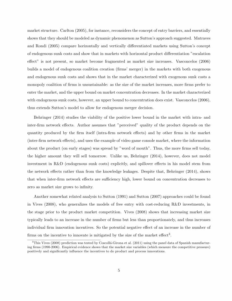
market structure. Carlton (2005), for instance, reconsiders the concept of entry barriers, and essentially

shows that they should be modeled as dynamic phenomenon as Sutton’s approach suggested. Matraves

and Rondi (2005) compare horizontally and vertically differentiated markets using Sutton’s concept

of endogenous sunk costs and show that in markets with horizontal product differentiation ”escalation

effect” is not present, so market become fragmented as market size increases. Vasconcelos (2006)

builds a model of endogenous coalition creation (firms’ merger) in the markets with both exogenous

and endogenous sunk costs and shows that in the market characterized with exogenous sunk costs a

monopoly coalition of firms is unsustainable: as the size of the market increases, more firms prefer to

enter the market, and the upper bound on market concentration decreases. In the market characterized

with endogenous sunk costs, however, an upper bound to concentration does exist. Vasconcelos (2006),

thus extends Sutton’s model to allow for endogenous merger decision.

Behringer (2014) studies the viability of the positive lower bound in the market with intra- and

inter-firm network effects. Author assumes that ”perceived” quality of the product depends on the

quantity produced by the firm itself (intra-firm network effects) and by other firms in the market

(inter-firm network effects), and uses the example of video game console market, where the information

about the product (on early stages) was spread by ”word of mouth”. Thus, the more firms sell today,

the higher amount they will sell tomorrow. Unlike us, Behringer (2014), however, does not model

investment in R&D (endogenous sunk costs) explicitly, and spillover effects in his model stem from

the network effects rather than from the knowledge leakages. Despite that, Behringer (2014), shows

that when inter-firm network effects are sufficiency high, lower bound on concentration decreases to

zero as market size grows to infinity.

Another somewhat related analysis to Sutton (1991) and Sutton (2007) approaches could be found

in Vives (2008), who generalizes the models of free entry with cost-reducing R&D investments, in

the stage prior to the product market competition. Vives (2008) shows that increasing market size

typically leads to an increase in the number of firms but less than proportionately, and thus increases

individual firm innovation incentives. So the potential negative effect of an increase in the number of

firms on the incentive to innovate is mitigated by the size of the market effect3.

3This Vives (2008) prediction was tested by Coscolla-Girona et al. (2011) using the panel data of Spanish manufactur-ing firms (1990-2006). Empirical evidence shows that the market size variables (which measure the competitive pressure)positively and significantly influence the incentives to do product and process innovations.

5

Concerning the related empirical literature, most of it focuses on testing for the presence of endoge-

nous sunk costs in an industry and its consequences for market concentration and competition and so

this literature is more relevant for our forthcoming analysis than the reviewed theoretical literature.

There is an important distinction between exogenous and endogenous sunk costs given their respective

role and impact on the the nature of competition in given markets (named Type I and Type II markets

respectively, following Schmalensee (1992)).

In the Type I markets, market size does not affect sunk costs. Therefore, as market grows more

firms enter the market, and market is likely to become more fragmented. On the other hand, increase

in the market size leads to an increase in the R&D expenditures (or other endogenous sunk costs)

by the incumbents on Type II markets who, in turn, create the barriers to entry for other firms, and

the market is more likely to remain concentrated. Thus, the predictions about the market size and

market concentration are clear in both cases: i) an increase in the market size in the exogenous sunk

costs markets does not influence R&D investment, but leads to new firm entry and decreased market

concentration; ii) in the endogenous sunk costs markets an increase in the market size leads to an

increase in R&D investment, and consequently limits or prevents the entry of new firms.

One of the examples of empirical tests of the endogenous sunk costs theory is the paper by Dick

(2007), which focuses on the banking industry. The author conjectures that the banking industry

is the endogenous sunk costs market. Using geographical definitions of the bank markets in USA

(defined by metropolitan statistical areas), the author finds that the correlation between market size

and concentration is close to zero, and provides evidence that banks invest extensively in quality to

raise the barriers to entry, which shows that banking industry are likely to be the Type II industry.

Furthermore, the paper investigates the quality provision in the banking industry. All quality measures

are positively associated with market size (advertising and branch intensity are among the measures

of quality), and so dominant banks in the markets provide higher quality than fringe banks.

Other empirical paper, testing endogenous sunk costs theory, is Robinson and Chiang (1996).

Authors use heterogeneous sample of consumer and industrial product markets and show that in

exogenous sunk costs markets minimum values of concentration decline towards zero as market size

increases, and in the endogenous sunk costs markets concentration remains bounded away from zero.

Similarly, Matraves (1999) finds that endogenous sunk costs play crucial role in pharmaceutical indus-

6

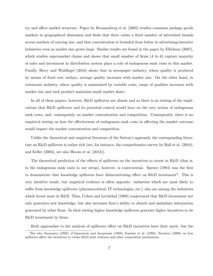
try and affect market structure. Paper by Bronnenberg et al. (2005) studies consumer package goods

markets in geographical dimension and finds that there exists a fixed number of advertised brands

across markets of varying size, and that concentration is bounded from below in advertising-intensive

industries even as market size grows large. Similar results are found in the paper by Ellickson (2007),

which studies supermarket chains and shows that small number of firms (4 to 6) capture majority

of sales and investment in distribution system plays a role of endogenous sunk costs in this market.

Finally, Berry and Waldfogel (2010) shows that in newspaper industry, where quality is produced

by means of fixed cost outlays, average quality increases with market size. On the other hand, in

restaurant industry, where quality is maintained by variable costs, range of qualities increases with

market size and each product maintains small market share.

In all of these papers, however, R&D spillovers are absent and so there is no testing of the impli-

cations that R&D spillovers and its potential control would have on the very notion of endogenous

sunk costs, and, consequently on market concentration and competition. Consequently, there is no

empirical testing on how the effectiveness of endogenous sunk costs in affecting the market outcome

would impact the market concentration and competition.

Unlike the theoretical and empirical literature of the Sutton’s approach, the corresponding litera-

ture on R&D spillovers is rather rich (see, for instance, the comprehensive survey by Hall et al. (2010),

and Keller (2004), see also Bloom et al. (2013)).

The theoretical prediction of the effects of spillovers on the incentives to invest in R&D (that is,

in the endogenous sunk costs in our setup), however, is controversial. Spence (1984) was the first

to demonstrate that knowledge spillovers have disincentivising effect on R&D investment4. This is

very intuitive result, but empirical evidence is often opposite: industries which are most likely to

suffer from knowledge spillovers (pharmaceutical, IT technologies, etc.) also are among the industries

which invest most in R&D. Thus, Cohen and Levinthal (1989) conjectured that R&D investment not

only generates new knowledge, but also increases firm’s ability to absorb and assimilate information

generated by other firms. In their setting higher knowledge spillovers generate higher incentives to do

R&D investment by firms.

Both approaches to the analysis of spillovers effect on R&D incentives have their merit, but the

4See also Suzumura (1992); d’Aspremont and Jacquemin (1988); Kamien et al. (1992); Tesoriere (2008) on howspillovers affect the incentives to create R&D joint ventures and other cooperation mechanisms.

7

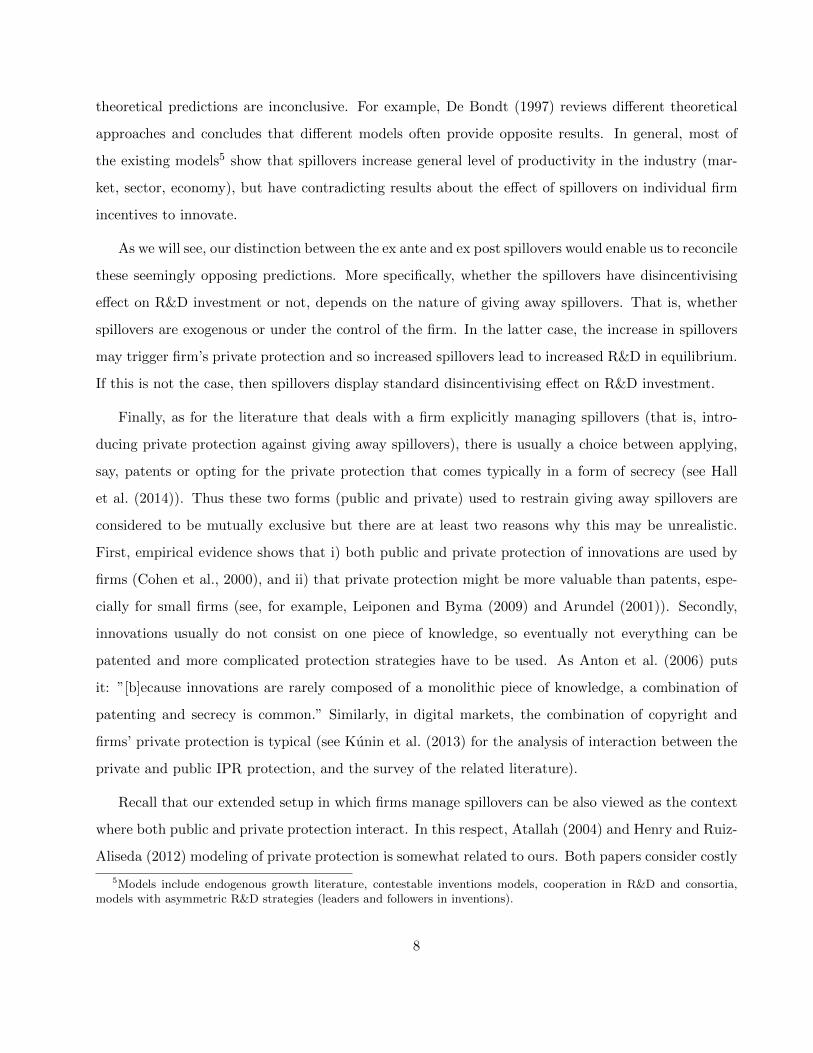
theoretical predictions are inconclusive. For example, De Bondt (1997) reviews different theoretical

approaches and concludes that different models often provide opposite results. In general, most of

the existing models5 show that spillovers increase general level of productivity in the industry (mar-

ket, sector, economy), but have contradicting results about the effect of spillovers on individual firm

incentives to innovate.

As we will see, our distinction between the ex ante and ex post spillovers would enable us to reconcile

these seemingly opposing predictions. More specifically, whether the spillovers have disincentivising

effect on R&D investment or not, depends on the nature of giving away spillovers. That is, whether

spillovers are exogenous or under the control of the firm. In the latter case, the increase in spillovers

may trigger firm’s private protection and so increased spillovers lead to increased R&D in equilibrium.

If this is not the case, then spillovers display standard disincentivising effect on R&D investment.

Finally, as for the literature that deals with a firm explicitly managing spillovers (that is, intro-

ducing private protection against giving away spillovers), there is usually a choice between applying,

say, patents or opting for the private protection that comes typically in a form of secrecy (see Hall

et al. (2014)). Thus these two forms (public and private) used to restrain giving away spillovers are

considered to be mutually exclusive but there are at least two reasons why this may be unrealistic.

First, empirical evidence shows that i) both public and private protection of innovations are used by

firms (Cohen et al., 2000), and ii) that private protection might be more valuable than patents, espe-

cially for small firms (see, for example, Leiponen and Byma (2009) and Arundel (2001)). Secondly,

innovations usually do not consist on one piece of knowledge, so eventually not everything can be

patented and more complicated protection strategies have to be used. As Anton et al. (2006) puts

it: ”[b]ecause innovations are rarely composed of a monolithic piece of knowledge, a combination of

patenting and secrecy is common.” Similarly, in digital markets, the combination of copyright and

firms’ private protection is typical (see Kunin et al. (2013) for the analysis of interaction between the

private and public IPR protection, and the survey of the related literature).

Recall that our extended setup in which firms manage spillovers can be also viewed as the context

where both public and private protection interact. In this respect, Atallah (2004) and Henry and Ruiz-

Aliseda (2012) modeling of private protection is somewhat related to ours. Both papers consider costly

5Models include endogenous growth literature, contestable inventions models, cooperation in R&D and consortia,models with asymmetric R&D strategies (leaders and followers in inventions).

8

investment by firms in making the product more complex and more complicated to copy. Henry and

Ruiz-Aliseda (2012) model R&D investment as invention race, with leading firms and several followers,

while Atallah (2004) considers R&D as non-tournament investment cost-decreasing investment, which

is more similar to our setup.

Like Atallah (2004), we show that public protection (patents) and private protection act as sub-

stitutes: the higher the level of ex ante (or exogenous) spillovers (that is, the lower the level of public

protection), the higher incentives to use costly private protection. Contrary to Atallah (2004), how-

ever, we show that investment in protection from spillovers is more likely if R&D investment becomes

less efficient. The reason for those difference is that we assume that R&D costs and protection costs

are interrelated. That is, decision to protect from spillovers increases R&D costs by some fraction,

unlike in Atallah (2004), where the costs of R&D and costs of protection are additively separable in

firms’ profit function. As a result, if R&D investments are less efficient, firms spend less on R&D, and

therefore protection is less costly. Moreover, as the consequence of lower barriers to entry (that is,

lower protection costs), more firms would enter the market. Clearly both factors point towards more

private protection.

Major difference of our approach from the related literature on knowledge spillover management

is, in general, that market structure (number of firms) is not given in our setup but it is, among other

things, the outcome of the interaction between the private and public protection from giving away

spillovers.

3 The Basic Model

3.1 Model setup

Much like Sutton (1991) or Sutton (2007) we also exploit essentially the same three-stage game setup

in our basic model. In the first stage firms decide whether or not to enter the market and the firms

that enter incur sunk entry cost, F0. In the second stage the firms choose sunk investment to set the

quality of the product, which we refer to as R&D investment. Finally, in the last stage, N firms which

entered the market simultaneously choose quantities, xi. The total cost of choosing quality level ui

for firm i is Fi = F0 + uβi , where ui is the quality level of good i, F0 is a setup cost, and β > 1 is a

9

model parameter that measures the effectiveness of R&D in raising perceived quality. A lower value

of β means that a given level of fixed R&D outlays leads to a greater increase in quality. When β

tends to infinity, R&D investment becomes more ineffective in enhancing quality. We consider R&D

investment as an instrument to produce product innovations (product quality), which are valued by

consumers. Due to spillovers, those innovations can be simultaneously developed by all firms in the

market and the examples of such a kind of product innovation could be, for instance, new models or

modifications of mobile phones, personal computers, or automobiles. Such kind of spillovers are coined

”output spillovers” (Hinloopen, 2000) since the competitors benefit from already achieved innovation

(”output”) rather than from investment in innovation that would instead imply ”input spillovers” (for

the distinction and the economic implications of the these two types of spillovers see Amir, 2000; Amir

et al., 2003).

Consumers, who are (as in Sutton, 1991, 2007) assumed to be homogenous in valuation of quality,

buy a good from firm i, based on the observed quality ui. A typical consumer’s utility function is of

the form

U = (ux)δz1−δ

where z is the outside good, and x is the ”quality” good, u ≥ 1 reflects the perception of good x′s

quality.

We start solving the model backward. Each firm offers a single good with quality ui at price pi.

Now, the consumer after observing prices and qualities of all firms, chooses to buy from the one, which

has the highest ui/pi ratio. For firms to have positive sales in equilibrium, we must have that

ui/pi = uj/pj for any i and j. (1)

With the given Cobb-Douglas form of utility function, let δ be the share of income spent on the

”quality” good (for derivations of that see Appendix A.1). Following the notation of Sutton (2007),

total spending on ”quality good” in the market S is such that S =N∑j=1

(pjxj). Note that S is the key

parameter that serves as the measure of the market size6. Also, we define ui/pi = uj/pj = 1/λ, where

λ can be interpreted as the price of good x with a unit quality. Now, if the price of a good x with a

6S can be also expressed asMδy, whereM is the measure of consumers in the market and y is income of a representativeconsumer.

10

unit quality is λ, the price of a good with quality ui is pi = λui = Sui/N∑j=1

(ujxj)7.

At the last stage of the game, investment in qualities are already sunk, and firms simultaneously

choose quantities to be sold to maximize profits. Firm i solves:

maxxi

Πi = pixi − cxi = λuixi − cxi

FOC(xi) : λui + uixidλ

dxi− c = 0

uixi =S

λ− cS

λ2ui

Summing up first-order conditions for all i = 1, ..., N, and rearranging it, we obtain profit expression

for firm i, after simultaneous choice of xi by each firm, as a function of quality choice ui:

Πi = S

1− N − 1

uiN∑j=1

(1/uj)

2

= S

1− N − 1

1 + ui∑j 6=i

(1/uj)

2

(2)

In the second stage, the firm i makes a decision about ui and faces the following choice: it can

stick with the basic quality level described with ui = 1, or invest in R&D and opt for higher quality

where ui > 1. In the former case, there is no R&D investment and thus no spillovers from other firms

since the basic quality is already known and well established, while in the latter case (setting ui to

ui > 1), the firm i chooses its investment in R&D and also benefits from the R&D of the other firms

via knowledge spillovers. We focus on the latter case that turns out to be relevant when market size

is ”large” enough.

Thus firms choose optimal level of investment in quality ui, while for consumers firm’s i perceived

product quality would be effectively u∗i ≥ ui. The reason for that are spillovers from other firms in the

industry. It is at this stage of the model, that we depart from Sutton’s original 3-stage game setup

and introduce knowledge spillovers to the model. Similar to Spence (1984) and Kamien et al. (1992),

7If we divide S by the total quantity of good x sold (weighed by quality),N∑j=1

(ujxj), then S/N∑j=1

(ujxj) = λ

11

we define u∗i in a linear way as

u∗i = ui +∑j 6=iθuj , (3)

where θ is an industry spillover parameter such that θ ∈ [0, 1). We denote the own quality choice by

firm i as ui, and uj is the quality choice by each of the other N − 1 firms. So firm’s i effective quality

comprises from the quality choice ui of the given firm i, and the fraction θ of the quality choices of

other firms, which enter u∗i through spillovers.

In other words, u∗i includes both the features and qualities developed by firm i, and some portion

of features and qualities developed independently by other firms in the market, and, as discussed in

the introduction, the channels via which this transfer of knowledge takes place are reverse-engineering,

labor force flows among firms, strategic alliances between firms, knowledge dispersion to competitors

through ”vertical channel” (supplier-client), etc.

With this definition of spillovers, the profit expression to be used in the second stage now becomes:

Πi = S

1− N − 1

u∗iN∑j=1

(1/u∗j )

2

= S

1− N − 1

1 + u∗i∑j 6=i

(1/u∗j )

2

(4)

When firm i makes a decision about ui, it compares the marginal benefit with the marginal cost

of the investment in quality.

The marginal benefit from investing in quality is:

dΠi

dui=∂Πi

∂u∗i

du∗idui

+∑j 6=i

∂Πi

∂u∗j

du∗jdui

(5)

Now,du∗idui

= 1 anddu∗jdui

= θ from (3). Deriving the expressions for ∂Πi∂u∗i

and ∂Πi∂u∗j

and imposing the

12

symmetry condition 8, we obtain expression for dΠidui

:

dΠi

dui=

2S(N − 1)2(1− θ)N3u(1 + (N − 1)θ)

(6)

Also, note that dFidui

= βuβ−1.

As we have argued above, for small market size, the investment in quality does not pay off. The

marginal benefit is then lower than marginal costs (that is, dΠidui

∣∣∣∣u=1

≤ dFidui

∣∣∣∣u=1

) so firms do not invest

in quality enhancing R&D and the standard quality ui = 1 prevails in the market equilibrium. As

a result, the number of firms is determined by exogenous fixed entry outlays, F0, and we label this

market setup as the exogenous sunk costs regime. As market size increases in this regime, more

firms enter the market, the market concentration decreases without a limit and, in the absence of

endogenous sunk costs, would approach zero as market size goes to infinity. Beyond a certain critical

value of S, (say, S), however, it may pay off for a firm to deviate and start investing in quality (that

is, to set, ui > 1)9. Thus, for market size large enough, profit maximization (with respect to u) may

require a shift to another, endogenous sunk cost regime that results in quality enhancing investment.

This would be exactly the case in our model (when spillovers are not ”too large”) so for S > S a firm

chooses ui > 1 by setting dΠidui

= dFidui

and this yields:

Fi =2S(N − 1)2(1− θ)N3β(1 + (N − 1)θ)

+ F0, (7)

which gives us optimal investment into quality for each firm in symmetric equilibrium, given N firms

entered 10.

Finally, to compute the number of firms entering in the first stage, we impose zero profit condition

(free entry): Fi = Πi. Expression for Πi in symmetric equilibrium becomes Πi = S(

1N

)2, with (7) we

8Symmetry condition which simplifies following expressions is ui = uj = u, yielding:

u∗i = ui +∑j 6=iθuj = u+ θ(N − 1)u = u(1 + (N − 1)θ);

u∗j = uj + θui +∑

k 6=i,k 6=jθuk = u+ θu+ θ(N − 2)u = u(1 + (N − 1)θ);

and u∗i = u∗j = u∗ = u(1 + (N − 1)θ).9Appendix A.5 provides an example how to calculate critical value S for certain parameter values.

10It is easy to demonstrate that d(dΠidui− dFi

dui

)/dui < 0 at ui = 2S(N∗−1)2(1−θ)

N∗3β(1+(N∗−1)θ)

1/β

. Therefore, the second order

condition is satisfied.

13

obtain:

2S(N − 1)2(1− θ)N3β(1 + (N − 1)θ)

+ F0 = S

(1

N

)2

(8)

The relation (8) above is an implicit equation for the optimal number of firms, N∗, from which we

can express N∗ as a function of market size S and parameters (F0, θ, β).

3.2 The lower bound of concentration, spillovers and the effectiveness of R&D

investment

The above analysis sets a stage to study how an interplay between spillovers, market size, and the

effectiveness of investment in quality improvement affects firms’ R&D outlays (that is, endogenous

sunk costs) and, consequently, equilibrium number of firms and market concentration under condition

of free entry. The effect of an increase in market size, S, on the endogenous sunk costs (in the absence

of spillovers) is already well known mainly due to the influential work of Sutton (1991; 2001; 2007).

Thus, the key insight of Sutton is that an increase in S leads to escalation of R&D expenditure and so

to the restrain of entry of new firms that in turn results in rather concentrated market even when the

market sizes grows without limit. Here we briefly discuss how these Sutton’s basic finding change once

we allow for spillovers among the firms. In this section we focus on the effects of spillovers on lower

bound of market concentration, while in the subsection 3.4 we look more closely at the interaction

between spillovers and the change in the endogenous sunk costs. We use the Herfindahl index, H as

the standard measure of market concentration that in the symmetric equilibrium assumes the value

H = 1/N∗. We rewrite (8) as:

F0

S=Nβ(1 + (N − 1)θ)− 2(N − 1)2(1− θ)

N3β(1 + (N − 1)θ)(9)

and it, in turn, enable us to state our first proposition.

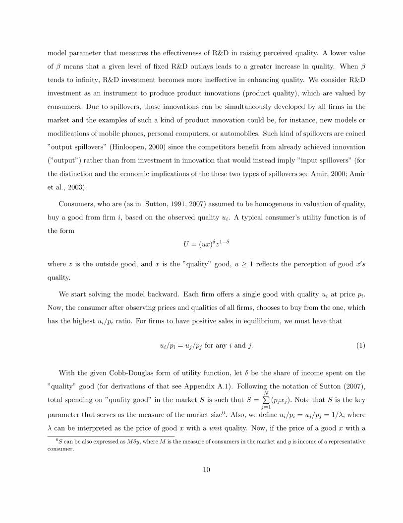
Proposition 1 An industry with low spillovers (that is, θ < 22+β ), for which endogenous sunk costs

matter, will, ceteris paribus, remain highly concentrated as size of the market increases, while an

industry with high spillovers will become fragmented with an increase in S.

14

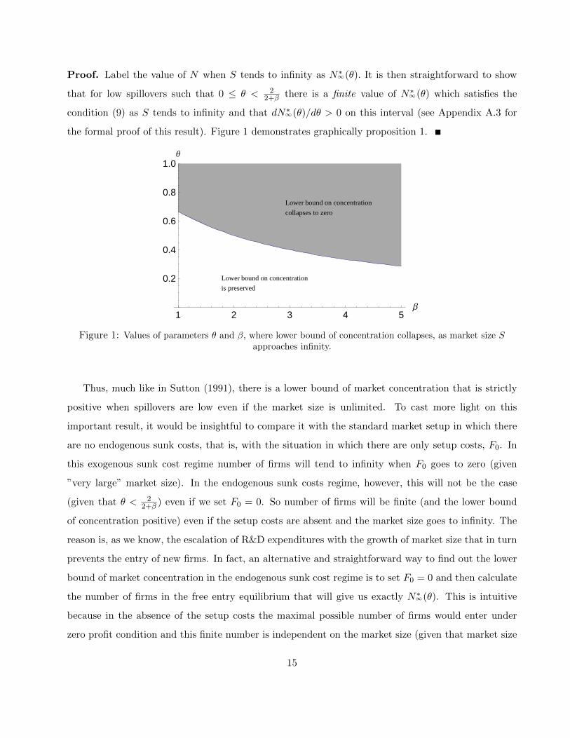
Proof. Label the value of N when S tends to infinity as N∗∞(θ). It is then straightforward to show

that for low spillovers such that 0 ≤ θ < 22+β there is a finite value of N∗∞(θ) which satisfies the

condition (9) as S tends to infinity and that dN∗∞(θ)/dθ > 0 on this interval (see Appendix A.3 for

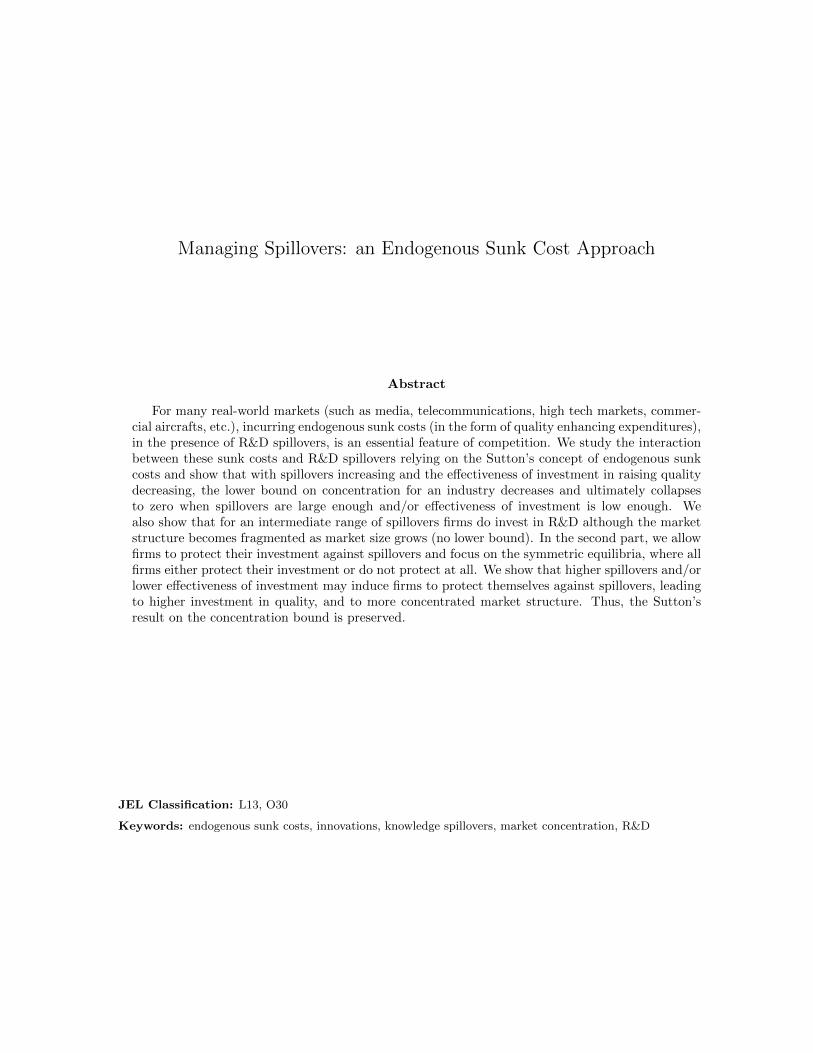
the formal proof of this result). Figure 1 demonstrates graphically proposition 1.

Lower bound on concentration

is preserved

Lower bound on concentration

collapses to zero

1 2 3 4 5Β

0.2

0.4

0.6

0.8

1.0Θ

Figure 1: Values of parameters θ and β, where lower bound of concentration collapses, as market size Sapproaches infinity.

Thus, much like in Sutton (1991), there is a lower bound of market concentration that is strictly

positive when spillovers are low even if the market size is unlimited. To cast more light on this

important result, it would be insightful to compare it with the standard market setup in which there

are no endogenous sunk costs, that is, with the situation in which there are only setup costs, F0. In

this exogenous sunk cost regime number of firms will tend to infinity when F0 goes to zero (given

”very large” market size). In the endogenous sunk costs regime, however, this will not be the case

(given that θ < 22+β ) even if we set F0 = 0. So number of firms will be finite (and the lower bound

of concentration positive) even if the setup costs are absent and the market size goes to infinity. The

reason is, as we know, the escalation of R&D expenditures with the growth of market size that in turn

prevents the entry of new firms. In fact, an alternative and straightforward way to find out the lower

bound of market concentration in the endogenous sunk cost regime is to set F0 = 0 and then calculate

the number of firms in the free entry equilibrium that will give us exactly N∗∞(θ). This is intuitive

because in the absence of the setup costs the maximal possible number of firms would enter under

zero profit condition and this finite number is independent on the market size (given that market size

15

is large enough to support endogenous sunk cost regime). That, in turn, yields the lower bound of

market concentration for F0 > 0 and market size tending to infinity.

For large spillovers, on the other hand, the market outcome is a bit different. When θ ≥ θ = 22+β ,

and as S goes to infinity, it has to be that the N∗∞(θ) also goes to infinity, in order for (9) to be satisfied.

In other words, N∗∞(θ) =∞. Thus the positive lower bound of concentration disappears11. The firm’s

sunk outlays, however, do not vanish once the spillovers reach or slightly exceed the threshold level,

θ, but become insufficient to block the new entry once the market size increases. So there is kind of

hybrid regime in which there are endogenous sunk costs on the one side, but the positive lower bound

of concentration vanishes, on the other side. Finally, at another, higher threshold of the spillover

level, θ > θ, the disincentives effect of spillovers prevails and is so strong that a firm opts for the

basic quality by setting ui = 1. The level of θ depends on the underlying parameters of the model,

that is, θ(β, S, F0) (see Appendix A.6 for the derivation of θ). Much like θ, it decreases in β, yielding

the lower critical level of spillovers beyond which there is a exogenous sunk cost regime (for given S

and F0). In addition, θ increases in S because larger market size gives motivation to invest more in

R&D so larger spillovers are needed to offset this incentive. Lastly and also intuitively, θ increases in

fixed entry costs since this increase, ceteris paribus, makes entry more difficult and therefore enhance

incentive to invest in R&D. In order to offset this, the critical level of spillovers θ has to increase.

Finally, it can be shown that limS→∞

θ = 2(1+F0)2(1+F0)+β < 1, so for the spillovers larger than this limit, there

is exogenous sunk cost regime irrespective of market size12.

We now switch for the moment to another important parameter of the model - the effectiveness of

R&D investment, β. First recall that β is an inverse measure of R&D effectiveness and this implies

that the larger β is, the lower will be investment in R&D investment. Consequently, when β tends

to infinity, a firm ceases to invest in R&D in the limit and sticks to basic quality ui = 1 (note that

limβ→∞

ui = 1).

11Moreover, N∗ approaches infinity at a different rate, depending on the value of the spillover parameter, with higherspillovers leading to a higher speed at which N∗increases.

12Nocke (2007), however, shows that large spillovers restore endogenous sunk cost regime in a particular dynamic modelin which firms compete in endogenous sunk outlays on quality and there is a collusive ”underinvestment” equilibriumwithout spillovers initially. So firms do not deviate from this equilibrium, because if one of them does it, the other firmsretaliate and also keep increasing their level of u from that time on. Such permanent escalation in sunk costs is verycostly and so not profitable compared to collusion but the appearance of large spillovers changes it completely. Theincentives to deviate is still present but the escalation of sunk costs will not be so costly because of spillovers. Thuspunishment would not be effective and therefore the ”underinvestment” equilibrium would not be sustained anymore (soonly the escalation equilibrium is possible).

16

Proposition 2 An industry, in which it would be easy to enhance the (perceived) product quality

(”low” β), would be more concentrated than an industry that has lower R&D effectiveness (”high” β)

given that both industries are exposed to the same ”low” level of spillovers (that is, θ < θ) and have

the same market size.

Proof. Note that both the critical levels of spillovers, θ and θ, depend on β; increase in β leads to a

fall in θ so the lower bound of concentration falls. By the same token, rise in β results in the fall of

θ and so, ceteris paribus, the exogenous sunk regime appears at the lower critical spillover level while

the associated market concentration is lower.

As expected, if R&D investment is not very effective in raising quality (β is high), firms do not

invest much in the R&D, and so barriers to entry are lower. In such circumstances a lower level of

spillovers is needed for the number of entrants to grow without limit as market size increases leading

the lower bound of concentration to collapse to zero.

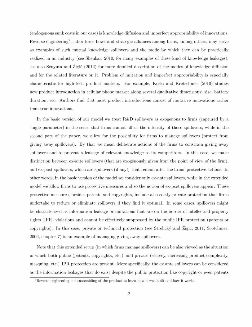
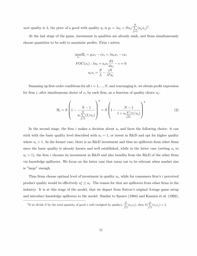
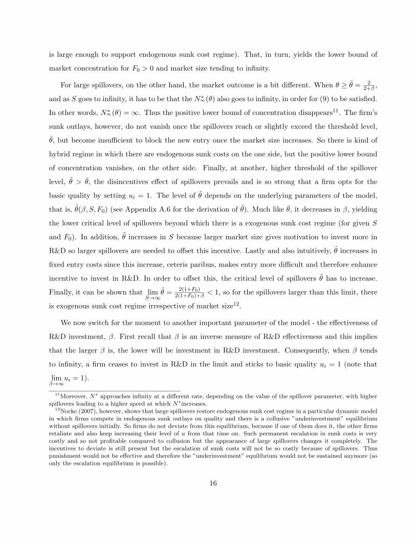
To illustrate how spillovers affect market concentration, we provide the numerical example below

(using parameter values β = 2, F0 = 2), and solve the model for the equilibrium N∗ for different values

of θ. The figure below demonstrates how the equilibrium concentration 1/N∗ and its lower bound

changes for different values of θ as market size S increases. For example, the upper line represents

the standard case when θ = 0, (spillovers are zero). For small S (dotted part of that curve), there is

exogenous sunk costs regime. For S high enough, there is endogenous sunk cost regime, lower bound

of market concentration approaches approximately 0.4, and the equilibrium number of firms is finite.

The lowest full line represents the case where θ = 0.7. Lower bound on concentration approaches zero

with S going to infinity, and equilibrium number of firms approaches infinity. So, with θ = 0.7 there

is an exogenous sunk cost regime for small S, and hybrid regime for S > 303. On the other hand, for

θ = 0.9 for any S we obtain exogenous sunk costs regime: for the assumed parameter values β and

F0, we have that 0.9 > θ, and we are in the exogenous sunk costs regime for all S.

As we can see from the parameterized example, the lower bound on equilibrium concentration level

(1/N∗) decreases with spillovers, and for the values of spillover parameter θ > θ = 22+β , it completely

disappears.

As for the empirical relevance of the above interplay between the market size, concentration,

spillovers and the lower bound of concentration, there are quite a few markets where endogenous sunk

17

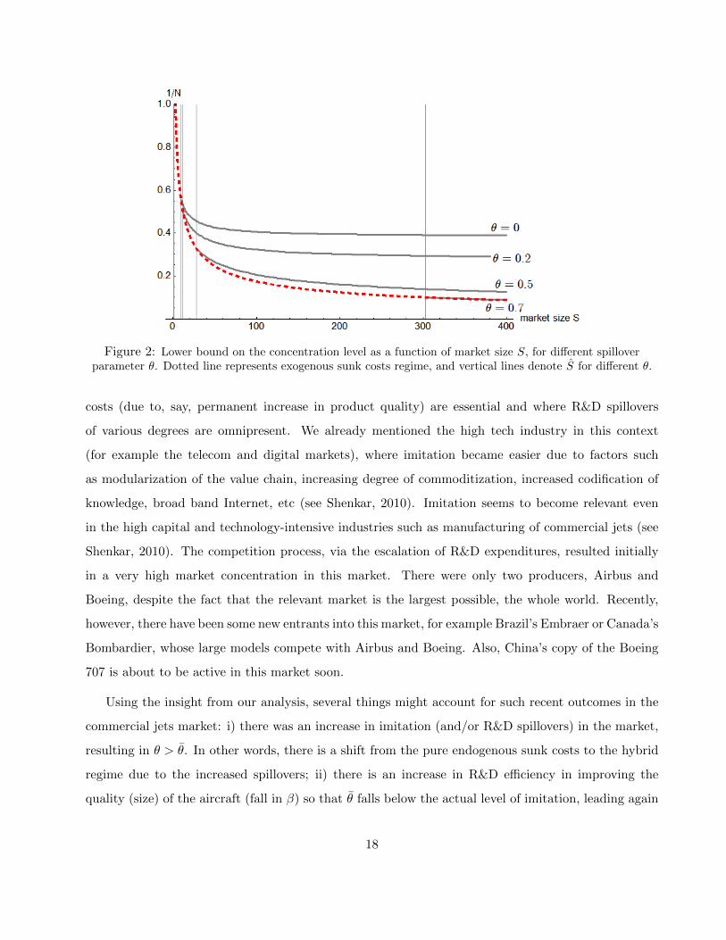
Figure 2: Lower bound on the concentration level as a function of market size S, for different spilloverparameter θ. Dotted line represents exogenous sunk costs regime, and vertical lines denote S for different θ.

costs (due to, say, permanent increase in product quality) are essential and where R&D spillovers

of various degrees are omnipresent. We already mentioned the high tech industry in this context

(for example the telecom and digital markets), where imitation became easier due to factors such

as modularization of the value chain, increasing degree of commoditization, increased codification of

knowledge, broad band Internet, etc (see Shenkar, 2010). Imitation seems to become relevant even

in the high capital and technology-intensive industries such as manufacturing of commercial jets (see

Shenkar, 2010). The competition process, via the escalation of R&D expenditures, resulted initially

in a very high market concentration in this market. There were only two producers, Airbus and

Boeing, despite the fact that the relevant market is the largest possible, the whole world. Recently,

however, there have been some new entrants into this market, for example Brazil’s Embraer or Canada’s

Bombardier, whose large models compete with Airbus and Boeing. Also, China’s copy of the Boeing

707 is about to be active in this market soon.

Using the insight from our analysis, several things might account for such recent outcomes in the

commercial jets market: i) there was an increase in imitation (and/or R&D spillovers) in the market,

resulting in θ > θ. In other words, there is a shift from the pure endogenous sunk costs to the hybrid

regime due to the increased spillovers; ii) there is an increase in R&D efficiency in improving the

quality (size) of the aircraft (fall in β) so that θ falls below the actual level of imitation, leading again

18

to a shift in regimes; and iii) the phenomena in both i) and ii) occur and reinforce each other. This

appears to be the most likely reason.

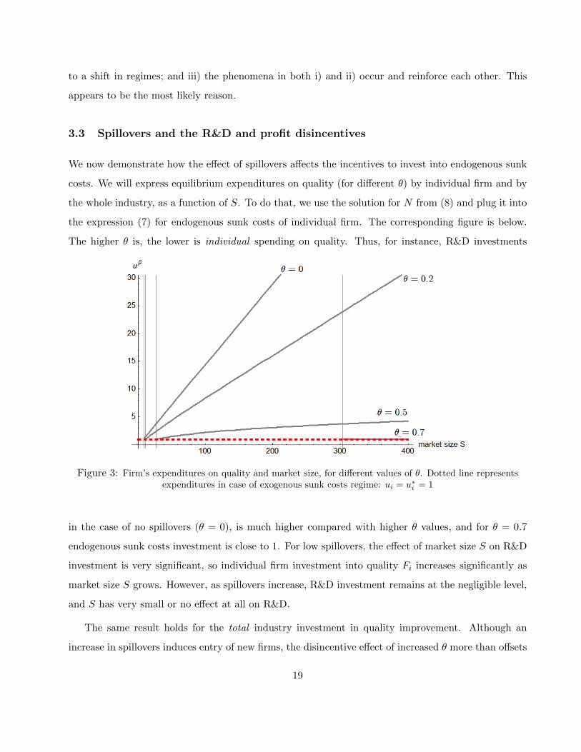
3.3 Spillovers and the R&D and profit disincentives

We now demonstrate how the effect of spillovers affects the incentives to invest into endogenous sunk

costs. We will express equilibrium expenditures on quality (for different θ) by individual firm and by

the whole industry, as a function of S. To do that, we use the solution for N from (8) and plug it into

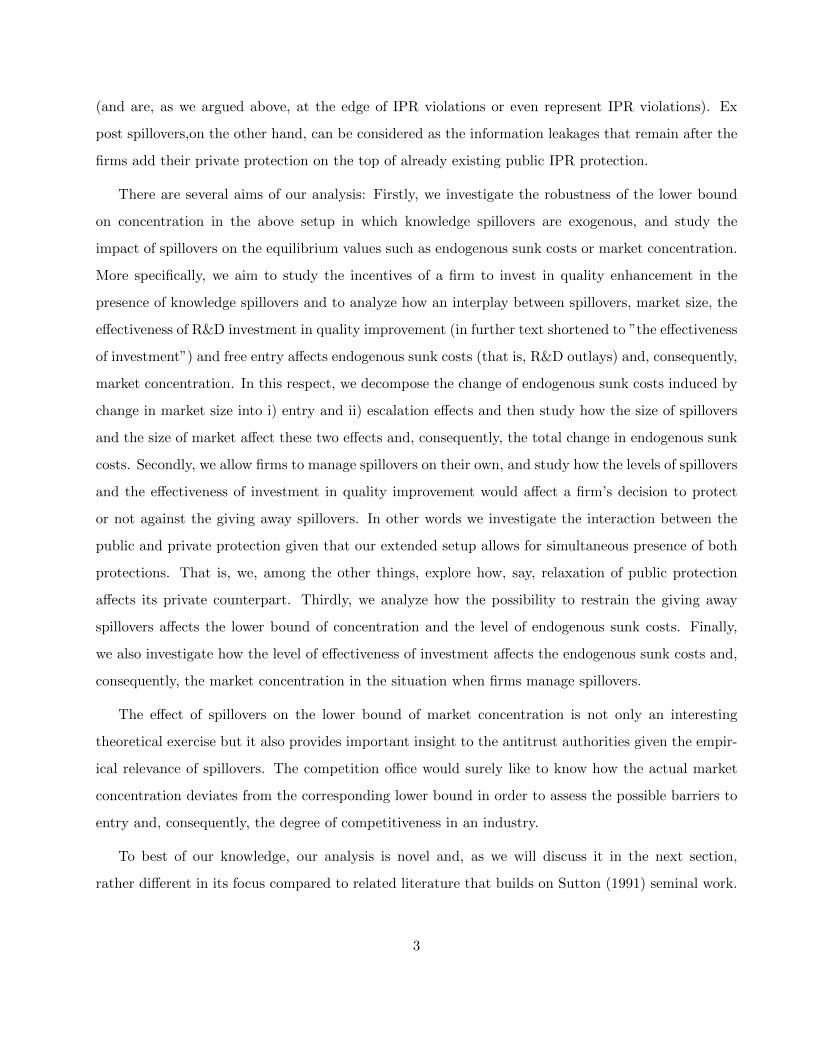
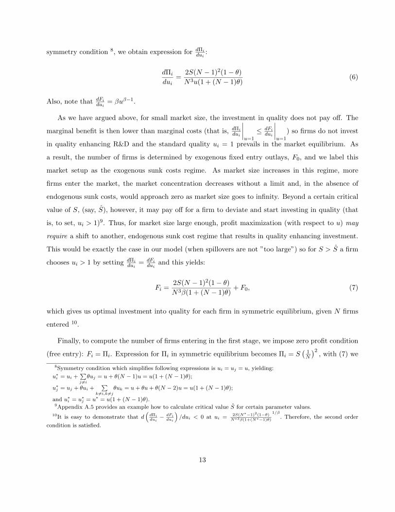
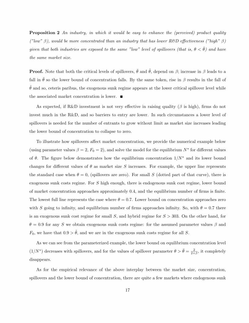
the expression (7) for endogenous sunk costs of individual firm. The corresponding figure is below.

The higher θ is, the lower is individual spending on quality. Thus, for instance, R&D investments

Figure 3: Firm’s expenditures on quality and market size, for different values of θ. Dotted line representsexpenditures in case of exogenous sunk costs regime: ui = u∗i = 1

in the case of no spillovers (θ = 0), is much higher compared with higher θ values, and for θ = 0.7

endogenous sunk costs investment is close to 1. For low spillovers, the effect of market size S on R&D

investment is very significant, so individual firm investment into quality Fi increases significantly as

market size S grows. However, as spillovers increase, R&D investment remains at the negligible level,

and S has very small or no effect at all on R&D.

The same result holds for the total industry investment in quality improvement. Although an

increase in spillovers induces entry of new firms, the disincentive effect of increased θ more than offsets

19

it so the total industry R&D investment falls as well. Thus, we would obtain an analogous graph for

the industry total R&D expenditure as that for the firm’s individual R&D investment. Therefore,

our next testable hypothesis is that the higher knowledge spillovers are, the lower R&D expenditures

are by both individual firm and an industry as a whole, other things being equal. In other words,

increasing the size of the market leads to an increase in R&D expenditure, but in the industries with

high spillovers this increase in R&D is happening at a much lower rate (if at all) than in the industries

with low spillovers.

The intuition for the above results, summarized in Figures 2 and 3, goes roughly as follows:

the impact of giving away spillovers becomes stronger than its receiving counterpart as the industry

spillover parameter rises. Each firm realizes that all other firms will free-ride on its investment, and

also it would be optimal to free-ride on others’ investment. Thus the consequence of rising spillovers

are decreasing endogenous sunk costs (see Figure 3), larger entry in the industry and, other things

being equal, lower market concentration (see Figure 2). Once spillovers surpass the threshold of

θ = 22+β , the disincentives to invest become so strong that the firms reduced their investment in R&D

so much that these investment cease to serve as the effective control of entry so that the lower bound

of concentrations disappears. That is, N∗ tends to infinity as market sizes increases.

Note also the disincentive effect that spillovers exhibit on a firm’s profit that we put in Lemma 1.

Lemma 1 As R&D spillovers increase, firm profits decline. That is, dΠidθ = ∂Πi

∂N∗dN∗

dθ + ∂Πi∂θ < 0.

This is in line with the empirical finding by Hanel and St-Pierre (2002) who show that information

spillovers negatively affect profits. Interestingly enough, the negative sign here does not come from

the direct effect of spillovers since it vanishes (that is, ∂Πi∂θ = 0) due to the symmetry in receiving

and giving away spillovers. Apparently, the key is in the indirect effect that turns out to be negative.

That is, the equilibrium profit declines in the number of firms while the equilibrium number of firms

increases with spillovers due to the mechanism described above (that is, ∂Πi∂N∗ < 0, and dN∗

dθ > 0; see

Appendix A.2 for the complete proof).

20

3.4 Endogenous versus exogenous sunk costs regimes: entry and escalation effects

We now aim to study how an interplay among spillovers, market size and free entry affects the firm’s

outlays on R&D. For that purpose, we decompose the change of endogenous sunk costs (dFi/dS)

into the direct and indirect effect. Thus, dFi/dS = (∂Fi/∂N) × (dN∗/dS) + ∂Fi/∂S where the first

part (∂Fi/∂N) × (dN∗/dS) stands for ”entry effect” while the second part (∂Fi/∂S), describes ”the

escalation effect” 13. The entry effect is typically negative and tells us what would be the change in

the endogenous sunk cost outlays of a firm due to entry of new firms induced by the increasing market

size14. More specifically, the increased size of the market would result in some entry that would in

turn negatively affect the investment in R&D due to the fact that the incentives to invest decrease

with more firms in the market.

The entry effect in our setup is ∂Fi∂N ×

dN∗

dS = F0S × f(N∗(S), θ, β), where f(N∗(S), θ, β) is the

function of the N∗ and the model parameters (see Appendix A.4).

Lemma 2 The entry effect tends to vanish as the market size goes to infinity and so the escalation

effect is the predominant one for the ”large” market given that spillovers are low (that, is 0 ≤ θ < θ).

As can be seen from the expression (A.3), the key determinant of the entry effect is the ratio of

setup costs to market size, F0/S, as it defines the ”capacity” for additional entry (see Appendix A.4

for more details). When, for instance, F0/S is low (say, due to large market size) there is already

”enough” firms in the market equilibrium so further decreases in this ratio makes room for smaller

and smaller additional entry. So as S approaches infinity, the ratio F0/S, goes to zero and in the limit

there is no space for any additional entry because all entry possibilities got exhausted. Thus entry

effect is of second-order importance for ”large markets” (since the ratio F0/S is then small). Moreover,

it would be completely absent when there are no set-up costs, F0, (that is, when F0 = 0, dN/dS = 0).

Recall that the total entry (in the limit) is comprised from either finite or infinite number of firms

depending on the spillovers level: for 0 ≤ θ < θ, there is the finite number of firms when S tends to

13Formally, ”escalation effect” and ”entry effect” are derived in the Appendix A.4.14It turns out that for very small or zero spillovers this derivative can be positive. As Vives (2008) showed, the entry

of new firms has two opposing effects on the R&D investment: the direct demand and the indirect price pressure effectsthat work in opposite directions. The direct demand effect typically dominates the price pressure effect, and R&Ddecreases with the number of firms. It is possible, however, that price pressure effect dominates the demand effect sothat an increase in the number of firms causes an increase in R&D expenditures (see the Appendix A.4 for more detaileddiscussion on this points).

21

infinity while for the spillover such that θ > θ, N goes to infinity as S goes to infinity.

As for the second, escalation effect, (unlike the entry effect), it does not depend on S so it does

not vanish in the limit when S tends to infinity provided that spillovers are low (that, is 0 ≤ θ < θ)

and is strictly positive.∂Fi∂S

=2(N∗ − 1)2(1− θ)

N∗3β(1 + (N∗ − 1)θ)> 0 (10)

Recall that the escalation effect, (when strong enough!) is at the heart of the non-fragmented market

structure and, consequently, a strictly positive lower bound of concentration15. This effect, however,

monotonically weakens with the rise of spillovers and for spillovers such that θ > θ, increase in market

size leads to an unlimited increase in number of firms, that, in turn, results in the zero escalation effect

in the limit, that is, limS→∞

∂Fi∂S

∣∣∣∣θ≥θ

= 0 (and, consequently, limS→∞

dFidS

∣∣∣∣θ≥θ

= 0, given that entry effect also

vanishes in the limit). Finally, at θ there is a switch to the exogenous sunk cost regime, as we saw,

and so the firms cease to invest in R&D (∂Fi∂S = 0 and so dFi/dS = 0 for θ ∈ [θ, 1)) irrespective of the

size of the market.

To conclude, the key factor in governing the total change of the sunk costs in the large markets

(small F0/S ratio) is the size of the escalation effect. The non-fragmented market structure appears

when spillovers are small (that, is 0 ≤ θ < θ). Beyond the critical level θ, however, the total effect,

dFi/dS, although positive, becomes ”too weak” to hold down the entry of new firms when the market

size increases. Thus, as we saw, for θ ∈ [θ, θ) there is a kind of hybrid regime: firms do invest in

R&D (that is, there are endogenous sunk costs), but, on the other hand, these investment do not

escalate when the market sizes grows. Instead the level of endogenous sunk costs barely changes but

the number of firms increase with the growing size of the market. In other words, there appears, like in

the exogenous sunk cost regime, fragmented market structure whereby market concentration tends to

zero. Apparently, spillovers and R&D act as the substitutes: the larger are mutual R&D spillovers the

lower R&D effort are needed to achieve the given level of perceived quality and so the firms curb R&D

when spillovers rise. Finally, for the spillovers level above θ, dFi/dS = 0, so there is exogenous sunk

costs in this case. Note that in the standard, Sutton (1991), setup without spillovers, the exogenous

sunk costs regime appears only for a ”small” market (when S < S), while in our setup the exogenous

sunk cost regime appears when θ > θ irrespective of the size of market.

15See Etro (2013) for an example where market concentration can even rise with the increase in market size.

22

Note that we could do the similar exercise, and decompose the effect of spillovers on a firm’s R&D

on its direct and indirect effects, that is, dFi/dθ = (∂Fi/∂N) × (dN∗/dθ) + ∂Fi/∂θ. Clearly, direct

effect of spillovers is negative due to the prevailing disincentive effect while the indirect effect is also

typically negative given that increase in spillovers makes entry easier (dN∗/dθ > 0) while presence of

more firms usually induce all firms to restrain their R&D outlays (∂Fi/∂N < 0) in equilibrium (see

Vives, 2008, and Appendix A.4).

4 Extended Model: Managing Spillovers

4.1 Model setup

Firms need to expect future profits (rents), in order to have incentives to invest in R&D but, as

we just saw, increased spillovers have a negative impact on a firm’s profit and R&D incentives so a

firm may consider the prevailing giving away spillovers to be excessive and may try to curb them.

In this light, one typically thinks of patents and copyrights as the means to prevent spillovers and

restore the incentives for innovation. Cohen and Levin (1989), however, provide an extensive review of

literature on effectiveness of patenting in different industries and come to the conclusion that in many

industries (machinery, electronics, food processing, etc.) only a negligible share of firms use patents16.

Instead, firms use other measures to protect R&D investment from spillovers like: secrecy, product

complexity, ability to learn quickly. As Shenkar (2010) noted ”. . . [L]egal protections have weakened at

the same time that codification, standardization, new manufacturing techniques, and growing employee

mobility making copying easier”. Also, Cohen et al. (2002) demonstrate that secrecy and lead time

appropriability mechanisms are more effective than patents in protecting innovations for firms in US.

Along the same line, Scotchmer (2006) defines so called private or technical IPR protection as an

alternative to legal patents. International trade literature (see, for example Taylor, 1993) refers to

physical ”masquing” techniques which are used by the producers who try to ensure the appropriability

of their product innovation.

So we now allow firms to use costly measures to privately protect their R&D investment from

16Mansfield (1986) shows that patent protection is important almost exclusively for innovations in pharmaceuticalindustry: 60% of innovations would not be developed without patent protection; while in other industries (machinery,metal, electrical equipment, instruments, motor vehicles, textiles) only between 0 and 15% if innovations would not bedeveloped without patent protection.

23

giving away spillovers. As we argued in the introduction, one situation when private protection

against spillovers may emerge is the case when adopting quality improvements of other firms by firm

i is at the edge of IPR violation and this would be especially the case if the public IPR protection is

not possible or, more likely, if it is not effective (say, due to enforceability problems, high litigation

costs, etc.). For instance, in the case when spillovers are realized through reverse-engineering17, such

a costly private protection measure would be making the product more complicated to disassemble

and copy. Atallah (2004) interprets this prevention of spillovers as any costly activity which enhances

secrecy of the product. If spillovers are realized through the labor force flows between firms, costly

private protection measures may mean that companies pay key employees more to prevent them from

leaving as, for instance, in Zabojnik (2002), Gersbach and Schmutzler (2003). They interpret the

costly prevention of spillovers as extra wages the workers are paid so that they do not leave the firm

and do not transfer important information to competitors; and in the case of receiving spillovers - this

is the extra wage the firm has to pay to the competitor’s workers to be able to hire them.

A somewhat different notion of endogenous spillovers than the one we use here was adopted in

the early literature on spillovers where endogenous spillovers typically mean that firms deliberately

fully or partially share their research output with each other. So firms cooperate in R&D by setting

research joint ventures or research consortia in which they endogenously and cooperatively set both

giving and receiving spillovers18.

Finally, note that unlike in the above literature on cooperation in R&D, the notion of endogenous

knowledge spillovers in our context has the meaning of unilaterally (non-cooperatively) curbing the

giving away spillovers.

By decreasing the spillover θ, firm i will also decrease the effective qualities of all other firms, which

will in turn have a positive effect on its profits (∂Πi∂u∗j

< 0 for all j 6= i).

In this section we assume that firms have an option to adopt costly protection against spillovers.

Thus, firms are able to restrain the size of spillovers if they find them too large and if this is not too

costly to do. For simplicity, we assume that firm i has a choice to decrease spillovers from θ to 0.

17Samuelson and Scotchmer (2002) describe legal issues related to reverse engineering, referring to it as appropriateand allowed industrial practice, and describes costly measures taken by firms to protect their product from such copying.

18The pioneering article in this sense was the Kamien et al. (1992), followed by Poyago-Theotoky (1999), Amir et al.(2003), and Tesoriere (2008). See also De Bondt (1997) for an early survey about the role of spillovers in R&D incentiveswho, among other things, noted that in reality spillovers are endogenous to a large extent, and possibly interacting withexogenous information leakages.

24

In this case, the costs would be Fi = F0 + αuβi , with α > 1, where α is a cost shifter that reflects

the fact that private protection of quality is costly as compared to costs Fi = F0 + uβi , when firm i

does not prevent spillovers19. On the benefit side, if firm i protects its investment from spillovers,

its effective quality remains the same (given that no other firm chooses to protect its investment):

u∗i = ui +∑j 6=iθuj , but the effective quality of all other firms decreases: u∗j = uj +

∑k 6=j, k 6=i

θuk, as

compared to u∗j = uj + θui +∑

k 6=j,k 6=iθuk.

We look for the set of parameters which satisfy the conditions for symmetric Nash equilibria,

where all firms either simultaneously choose to protect their investment from spillovers, or they do

not protect.

The timing of the model is much like in the previous section, with one more step introduced. In

the first stage firms decide whether or not to enter the market, in the second stage, the firms that

entered pay sunk entry cost, F0, and also choose sunk investment in quality of the product. In the

third stage firms decide whether to protect their investment from spillovers or not. Note that sunk

costs investment and protection decisions are taken at different stages (see, for example, Gersbach and

Schmutzler, 2003; Atallah, 2004, for similar timing). Such ”sequential” setup implies that firms, while

deciding on the protection, observe the level of R&D investment of their competitors. Finally, in the

last stage, N firms which entered the market simultaneously choose quantities, xi.

First, consider the equilibrium where all firms choose to manage spillovers. Given that all firms

have chosen protection (implying that θ = 0), the firms choose optimally investment level into quality.

For this equilibrium to be well defined, the firms, as we know, have to operate in the endogenous sunk

costs regime. That is, the market size has to be large enough (S ≥ S) and we assume that this is the

case. (For instance, for β = 2, F0 = 2, θ = 0, market size has to be such that S ≥ S = 8.5)20.

From (6), we obtain that dΠidui

= 2S(N−1)2

N3u, and dFi

dui= βαuβ−1. Profit maximization requires that

dΠidui

= dFidui, and by symmetry assumption, uβ = 2S(N−1)2

N3β α. Much as in the previous section, we have

the zero-profit condition,

α2S(N − 1)2

N3βα+ F0 = S

(1

N

)2

(11)

19See Taylor (1993) for the related definition of the cost function of a firm which adopts ”masquing” techniques toprevent or make giving away spillovers more difficult.

20For details on deriving S, see Appendix A.5.

25

that determines the number of firms which enter the market in ”protection” equilibrium.

Now, assume that a firm i decides to deviate and stops protecting from spillovers at stage 3. Profit

expression for firm i changes to:

ΠDi = S

1− (N − 1)

1 + u∗i∑j 6=i

(1/u∗j )

2

where u∗i = ui, and for all other firms u∗j = uj + θui. Now, with this symmetry assumption profit

expression becomes:

ΠDi = S

((2−N)θ + 1

N + θ

)2

< S

(1

N

)2

The cost expression for a deviant firm i becomes FDi = F0 + uβ = F0 + 2S(N−1)2

N3β α. Now, if

ΠDi − FDi = S

((2−N)θ + 1

N + θ

)2

− F0 −2S(N − 1)2

N3β α≤ 0, (12)

where N is the solution to implicit equation (11), firm i does not have incentives to deviate from sym-

metric equilibria, where all firms protect against spillovers. This means that for θ ≥ θ(β) symmetric

protection equilibrium can be sustained, where θ(β) is determined by (12) which holds with equality.

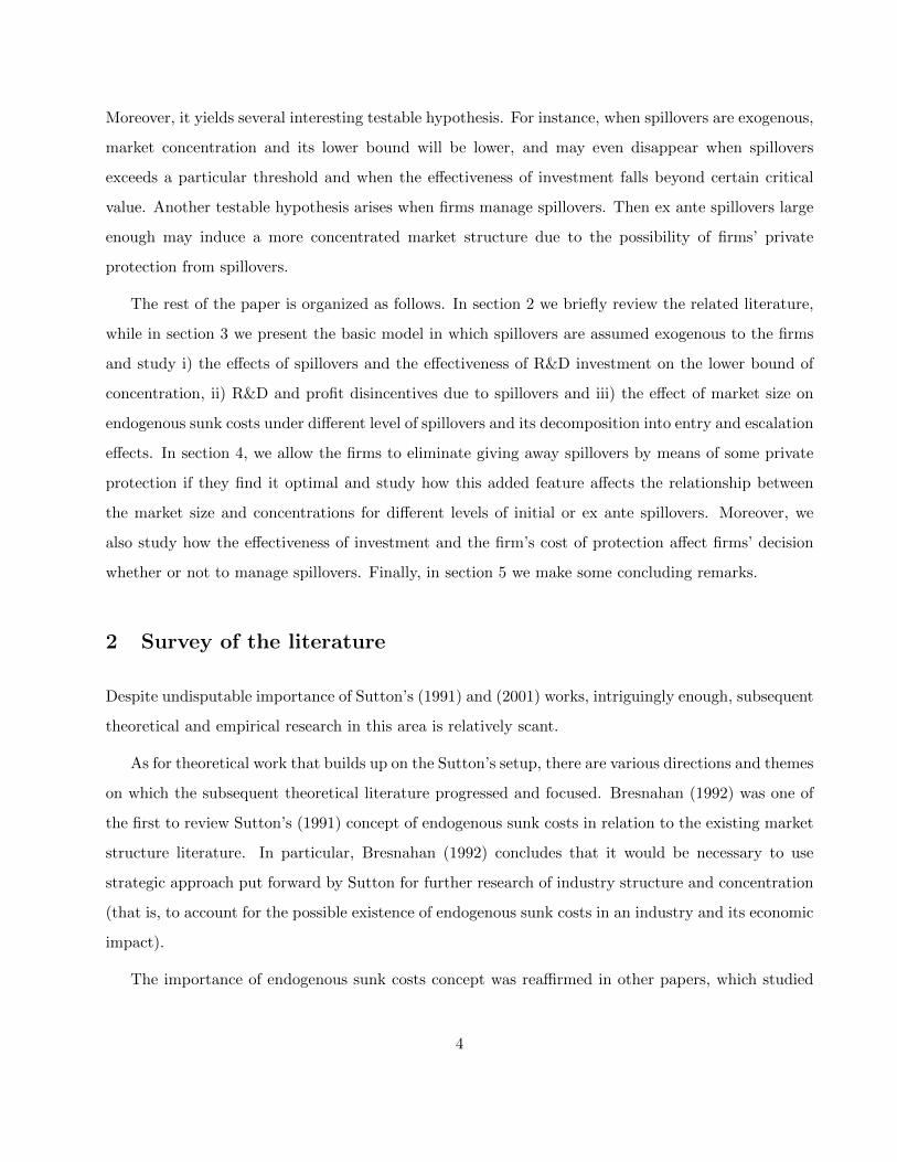
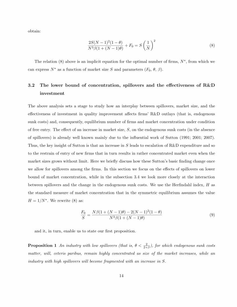
We demonstrate the solution to inequality (12) with a numerical example. For the parameter

values (S = 100, F0 = 2), we define such a combination of values of spillover θ and investment cost

parameter β, that (12) holds. On the Figure 4 below, the dashed area defines the set of parameters β

and θ, for which ”protection” equilibrium will exist. We can see that for high enough spillovers firms

will not deviate from protection. There is a critical level of spillovers, θ(β), represented by the lower

bound of the dashed area on Figure 4, above which the protection regime is sustained.

Now, consider the equilibrium where none of the firms use protection against spillovers. As in the

previous section, (7) defines costs of investment for firm i, and profit is S(

1N

)2. Now, assume that a

firm i decides to deviate and starts protecting from spillovers at stage 3. Profit expression for firm i

26

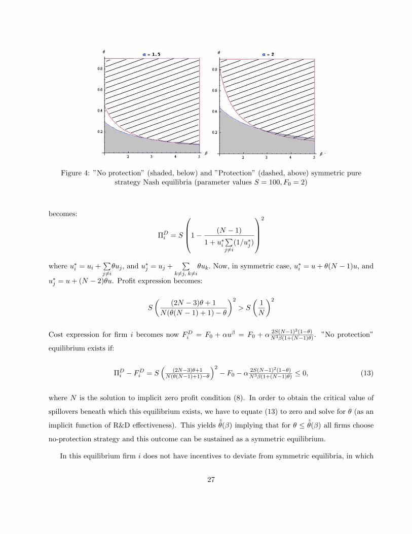
Figure 4: ”No protection” (shaded, below) and ”Protection” (dashed, above) symmetric purestrategy Nash equilibria (parameter values S = 100, F0 = 2)

becomes:

ΠDi = S

1− (N − 1)

1 + u∗i∑j 6=i

(1/u∗j )

2

where u∗i = ui +∑j 6=iθuj , and u∗j = uj +

∑k 6=j, k 6=i

θuk. Now, in symmetric case, u∗i = u+ θ(N − 1)u, and

u∗j = u+ (N − 2)θu. Profit expression becomes:

S

((2N − 3)θ + 1

N(θ(N − 1) + 1)− θ

)2

> S

(1

N

)2

Cost expression for firm i becomes now FDi = F0 + αuβ = F0 + α 2S(N−1)2(1−θ)N3β(1+(N−1)θ)

. ”No protection”

equilibrium exists if:

ΠDi − FDi = S

((2N−3)θ+1

N(θ(N−1)+1)−θ

)2− F0 − α 2S(N−1)2(1−θ)

N3β(1+(N−1)θ)≤ 0, (13)

where N is the solution to implicit zero profit condition (8). In order to obtain the critical value of

spillovers beneath which this equilibrium exists, we have to equate (13) to zero and solve for θ (as an

implicit function of R&D effectiveness). This yields ˆθ(β) implying that for θ ≤ ˆθ(β) all firms choose

no-protection strategy and this outcome can be sustained as a symmetric equilibrium.

In this equilibrium firm i does not have incentives to deviate from symmetric equilibria, in which

27

none of the firms protects from spillovers. In the Figure 4 above the shaded area defines the set

of parameters β and θ, for which (13) holds and ”no protection” equilibrium exist (for S = 100,

α = {1.5; 2}, F0 = 2).

Proposition 3 For ex ante spillovers such that θ ≥ θ(β) there exists a symmetric ”protection” equi-

librium. That is, all firms in an industry adopt protection (resulting in zero ex post spillovers) and

no single firm has unilateral incentive to deviate to ”no protection” strategy. If, however, θ < ˆθ(β)

then no single firm has an incentive to unilaterally adopt protection strategy and thus ”no protection”

equilibrium could be sustained as a symmetric equilibrium. Moreover there is no difference between the

ex ante and ex post spillovers in this case.

For spillovers low enough, firms will not undertake costly protection measures. The reason is that

costs of protection (in terms of higher R&D expenditures) do not directly depend on the level of

spillovers, but the benefits (in terms of profit gain) do. So if spillovers are low, benefits of starting

protection (or alternatively, the loss of profit because of not protecting) are low compared to incurred

costs of protection. Note, further, that the critical values of spillovers depend on the effectiveness of

R&D. For high enough values of β firms would tolerate only very small spillovers and so the range of

parameter θ for which no-protection equilibrium would exists, becomes smaller as β increases. The

reason for that is that the low effectiveness of R&D (high β), leads to low endogenous sunk cost (see

the expression 7) and to more firms entering the market. With more firms in the market, the benefit

from protection rises, and a firm is willing to undertake it even for small spillovers.

It is insightful to interpret the above story in the context of the interaction between the public

and the private protection. When public protection is ”lax enough” (that is, when θ ≥ θ(β)), it

triggers private protection that eliminates giving away spillovers. Thus, private and public protection

become ”complements” to each other once the threshold spillovers level has been reached and the

protection equilibrium occurs then. For the ex- ante spillovers that are below a threshold level, firms,

however, do not use private protection but rely instead on the (imperfect) public protection that serves

as a substitute for the costly private protection, and so there is no-protection equilibrium outcome.

Moreover, the lower is the efficiency of R&D investment (that is, the larger is β), the easier is to

induce private protection (that is, even relatively strong but not perfect public protection triggers

private protection when β is large).

28

Much like in the case of protection equilibria, for ”no protection” equilibrium to be well defined,

the firms have to invest in R&D (that is, they have to operate in either endogenous or hybrid regime).

Thus, the level of spillovers in the case of no protection equilibrium has to be beneath the critical level

θ in order to preclude the exogenous sunk cost regime (see Figure 4). Moreover, for a ”no protection”

equilibrium to exist, the necessary condition is that spillovers have to be low enough not to trigger

the protection, that is, θ < θ(β)21.

For the values of parameters that are not in the shaded or dashed areas (intermediate θ and low β

values), there is no symmetric equilibrium in pure strategies. For such values of parameters if all firms

protect, there are always incentives for one firm to deviate to ”no protection”. On the other hand,

if all firms do not protect, a firm always has incentives to deviate from ”no protection” behavior and

starts protecting its quality features. Also, there is an area (where dashed and shaded areas intersect)

on the Figure 4 above where both ”protection” and ”non protection” equilibria exist. That is, if all

firms choose to protect their investment from spillovers, each single firm would not prefer to deviate

to not protecting; on the other hand, if all firms choose not to protect, each single firm would not

prefer to deviate and start protecting.

Also, as α increases from 1.5 to 2, ”no protection” (shaded) area become larger - it is now more

costly to protect against spillovers, and ”no protection” equilibrium is more likely, other things being

equal. On the contrary, the ”protection” (dashed) area shrinks as it becomes more costly to protect.

4.2 The lower bound of concentration when spillovers are managed

As Figure 4 demonstrates, for different values of θ different equilibria will emerge. In the following

analysis we fix cost parameters β = 2, α = 2, F0 = 2, and draw the concentration schedule as a

function of market size for different θ (Figure 5).

For θ = 0 and θ = 0.2, we have ”no protection” equilibria, and the concentration versus market

size schedule is the same as in Figure 2. However, for higher values of θ ”protection” equilibria will

emerge, meaning that firms will choose to manage spillovers and decrease them to zero. For these cases

concentration versus market size schedule coincides with the upper curve in Figure 2. As a result, we

21Note that for ”no protection” equilibrium to be well defined, θ < θ has to hold and this is always the case in oursetup, if market size S is large enough.

29

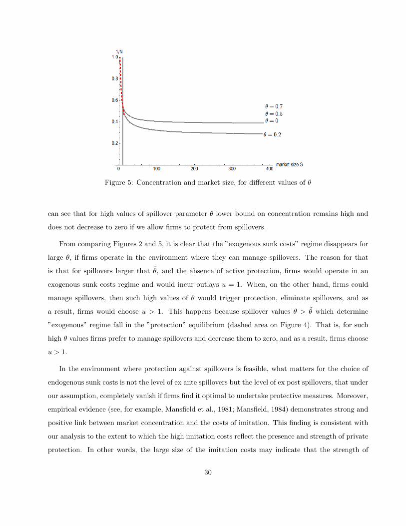
Figure 5: Concentration and market size, for different values of θ

can see that for high values of spillover parameter θ lower bound on concentration remains high and

does not decrease to zero if we allow firms to protect from spillovers.

From comparing Figures 2 and 5, it is clear that the ”exogenous sunk costs” regime disappears for

large θ, if firms operate in the environment where they can manage spillovers. The reason for that

is that for spillovers larger that θ, and the absence of active protection, firms would operate in an

exogenous sunk costs regime and would incur outlays u = 1. When, on the other hand, firms could

manage spillovers, then such high values of θ would trigger protection, eliminate spillovers, and as

a result, firms would choose u > 1. This happens because spillover values θ > θ which determine

”exogenous” regime fall in the ”protection” equilibrium (dashed area on Figure 4). That is, for such

high θ values firms prefer to manage spillovers and decrease them to zero, and as a result, firms choose

u > 1.

In the environment where protection against spillovers is feasible, what matters for the choice of

endogenous sunk costs is not the level of ex ante spillovers but the level of ex post spillovers, that under

our assumption, completely vanish if firms find it optimal to undertake protective measures. Moreover,

empirical evidence (see, for example, Mansfield et al., 1981; Mansfield, 1984) demonstrates strong and

positive link between market concentration and the costs of imitation. This finding is consistent with

our analysis to the extent to which the high imitation costs reflect the presence and strength of private

protection. In other words, the large size of the imitation costs may indicate that the strength of

30

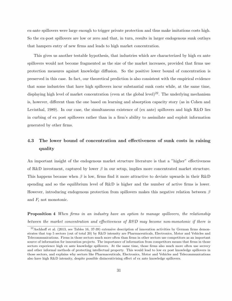
ex-ante spillovers were large enough to trigger private protection and thus make imitations costs high.

So the ex-post spillovers are low or zero and that, in turn, results in larger endogenous sunk outlays

that hampers entry of new firms and leads to high market concentration.

This gives us another testable hypothesis, that industries which are characterized by high ex ante

spillovers would not become fragmented as the size of the market increases, provided that firms use

protection measures against knowledge diffusion. So the positive lower bound of concentration is

preserved in this case. In fact, our theoretical prediction is also consistent with the empirical evidence

that some industries that have high spillovers incur substantial sunk costs while, at the same time,

displaying high level of market concentration (even at the global level)22. The underlying mechanism

is, however, different than the one based on learning and absorption capacity story (as in Cohen and

Levinthal, 1989). In our case, the simultaneous existence of (ex ante) spillovers and high R&D lies

in curbing of ex post spillovers rather than in a firm’s ability to assimilate and exploit information

generated by other firms.

4.3 The lower bound of concentration and effectiveness of sunk costs in raising

quality

An important insight of the endogenous market structure literature is that a ”higher” effectiveness

of R&D investment, captured by lower β in our setup, implies more concentrated market structure.

This happens because when β is low, firms find it more attractive to deviate upwards in their R&D

spending and so the equilibrium level of R&D is higher and the number of active firms is lower.

However, introducing endogenous protection from spillovers makes this negative relation between β

and Fi not monotonic.

Proposition 4 When firms in an industry have an option to manage spillovers, the relationship

between the market concentration and effectiveness of R&D may become non-monotonic if there is

22Aschhoff et al. (2013, see Tables 16, 37-39) extensive description of innovation activities by German firms demon-strates that top 5 sectors (out of total 20) by R&D intensity are Pharmaceuticals, Electronics, Motor and Vehicles andTelecommunications. Firms in those sectors much more often than firms in other sectors use competitors as an importantsource of information for innovation projects. The importance of information from competitors means that firms in thosesectors experience high ex ante knowledge spillovers. At the same time, those firms also much more often use secrecyand other informal methods of protecting intellectual property. This would lead to low ex post knowledge spillovers inthose sectors, and explains why sectors like Pharmaceuticals, Electronics, Motor and Vehicles and Telecommunicationsalso have high R&D intensity, despite possible disincentivising effect of ex ante knowledge spillovers.

31

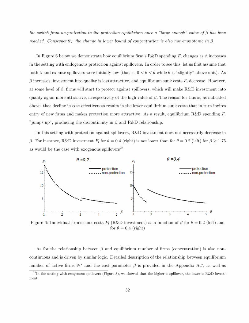
the switch from no-protection to the protection equilibrium once a ”large enough” value of β has been

reached. Consequently, the change in lower bound of concentration is also non-monotonic in β.

In Figure 6 below we demonstrate how equilibrium firm’s R&D spending Fi changes as β increases

in the setting with endogenous protection against spillovers. In order to see this, let us first assume that

both β and ex ante spillovers were initially low (that is, 0 < θ < θ while θ is ”slightly” above unit). As

β increases, investment into quality is less attractive, and equilibrium sunk costs Fi decrease. However,

at some level of β, firms will start to protect against spillovers, which will make R&D investment into

quality again more attractive, irrespectively of the high value of β. The reason for this is, as indicated

above, that decline in cost effectiveness results in the lower equilibrium sunk costs that in turn invites

entry of new firms and makes protection more attractive. As a result, equilibrium R&D spending Fi

”jumps up”, producing the discontinuity in β and R&D relationship.

In this setting with protection against spillovers, R&D investment does not necessarily decrease in

β. For instance, R&D investment Fi for θ = 0.4 (right) is not lower than for θ = 0.2 (left) for β ≥ 1.75

as would be the case with exogenous spillovers23.

Figure 6: Individual firm’s sunk costs Fi (R&D investment) as a function of β for θ = 0.2 (left) andfor θ = 0.4 (right)

As for the relationship between β and equilibrium number of firms (concentration) is also non-

continuous and is driven by similar logic. Detailed description of the relationship between equilibrium

number of active firms N∗ and the cost parameter β is provided in the Appendix A.7, as well as

23In the setting with exogenous spillovers (Figure 3), we showed that the higher is spillover, the lower is R&D invest-ment.

32

corresponding graphs.

Therefore, our last testable hypothesis relates R&D expenditures (and market concentration) to

the effectiveness of those expenditures, in the sense that lower effectiveness of R&D expenditures

(higher β) would not lead to lower endogenous sunk costs if the firm starts to use costly protection

against spillovers for higher values of β. Moreover, if ex ante spillovers are high, firms are more likely to

use protection against spillovers even for effective R&D expenditures (low β). This would lead to even

higher R&D expenditures (because of curbed spillovers and low β), and an even more concentrated

market structure.

5 Concluding Remarks

We used a simple version of the Sutton (2007) model that illustrates the economic consequences

of endogenous sunk costs on firms’ entry and market concentration and extended it by allowing for

spillovers stemming from firms’ investment in product quality. In the first part of our paper, we assume

that spillovers are exogenous to the firms. As expected (in this setup), spillovers tend to decrease the

lower bound of market concentration and when strong enough completely eliminate it. Eliminating the

lower bound does not, however, imply immediate elimination of a firm incurring endogenous sunk costs

nor, consequently, switch to the exogenous sunk costs regime. We showed that for an intermediate

range of spillovers, θ ∈ [θ, θ), firms do invest in R&D although the market concentration becomes

fragmented as market size grows (that is, there is no positive lower bound). Finally, for very large

spillovers, (θ > θ), firms do not invest in quality improvement due to very strong disincentive effects

of spillovers. In other words, potential leakages of information in the industry is so large that firms

refrain from R&D so that spillovers do not become materialized at all. The effectiveness of R&D

investment plays a key role in determining both threshold levels of spillovers beyond which lower

bound disappears, θ, and beyond which the exogenous sunk cost regime appears, θ. The testable

hypothesis, given exogenous spillovers assumption, is that market concentration and its lower bound

will be lower when spillovers are higher and the effectiveness of investment in raising quality is lower.

In the second part we allow firms to protect their investment against spillovers, if it would be

optimal for them. We focus on symmetric pure strategy Nash equilibria, where all firms either protect

their investment or not. As a result, for different values of parameters different equilibria may arise. For

33

low values of θ ”no protection” equilibrium exists while for high enough values of θ and β ”protection”

equilibrium occurs. Contrary to the case of exogenous spillovers, we show that ex ante spillovers

may lead to a more concentrated market structure due to the possibility of firms’ private protection

from spillovers, and this represents another testable hypothesis. It also suggests the related testable

hypothesis that lower effectiveness of raising quality (higher β) does not lead to lower endogenous sunk

costs, and, consequently, to lower market concentration if it triggers firms to use costly protection

against spillovers.

We also show that the framework in which firms manage spillovers can be viewed as the situation

where both public and private protections are present and that, in turn, enables one to study the

economic interaction of the two forms of protection.

Finally, it is worth stressing that our paper is related to three separate topics in industrial organi-

zation literature: i) innovation and R&D incentives, ii) market structure and iii) knowledge spillovers.

While the related literature usually studies all three notions separately, commonly assuming mar-

ket structure and R&D spillovers as exogenous parameters, we put forward a theoretical model that

simultaneously and endogenously determines the equilibrium values of all three features under consid-

erations.

34

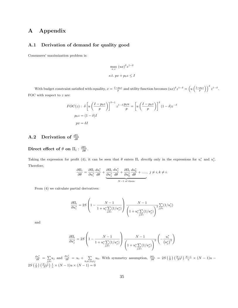
A Appendix

A.1 Derivation of demand for quality good

Consumers’ maximization problem is:

maxx,z

(ux)δz1−δ

s.t. px+ p0z ≤ I

With budget constraint satisfied with equality, x = I−p0zp

and utility function becomes (ux)δz1−δ =(u(I−p0zp

))δz1−δ.

FOC with respect to z are:

FOC(z) : δ

[u

(I − p0z

p

)]δ−1

z1−δ p0u

p=

[u

(I − p0z

p

)]δ(1− δ)z−δ

p0z = (1− δ)I

px = δI

A.2 Derivation of dΠidθ

Direct effect of θ on Πi : ∂Πi∂θ .

Taking the expression for profit (4), it can be seen that θ enters Πi directly only in the expressions for u∗i and u∗j .

Therefore,∂Πi

∂θ=∂Πi

∂u∗i

du∗idθ

+∂Πi

∂u∗j

du∗jdθ

+∂Πi

∂u∗k

du∗kdθ

+ .....︸ ︷︷ ︸N−1 of them

, j 6= i, k 6= i.

From (4) we calculate partial derivatives:

∂Πi

∂u∗i= 2S

1− N − 1

1 + u∗i∑j 6=i

(1/u∗j )

N − 1(1 + u∗i

∑j 6=i

(1/u∗j )

)2

∑j 6=i

(1/u∗j )

and

∂Πi

∂u∗j= 2S

1− N − 1

1 + u∗i∑j 6=i

(1/u∗j )

N − 1(1 + u∗i

∑j 6=i

(1/u∗j )

)2

(− u∗i(

u∗j)2)

du∗idθ

=∑j 6=iuj and

du∗jdθ

= ui +∑

k 6=i,k 6=juk. With symmetry assumption, ∂Πi

∂θ= 2S

(1N

) (N−1N2

)N−1u× (N − 1)u −

2S(

1N

) (N−1N2

)1u× (N − 1)u× (N − 1) = 0

35

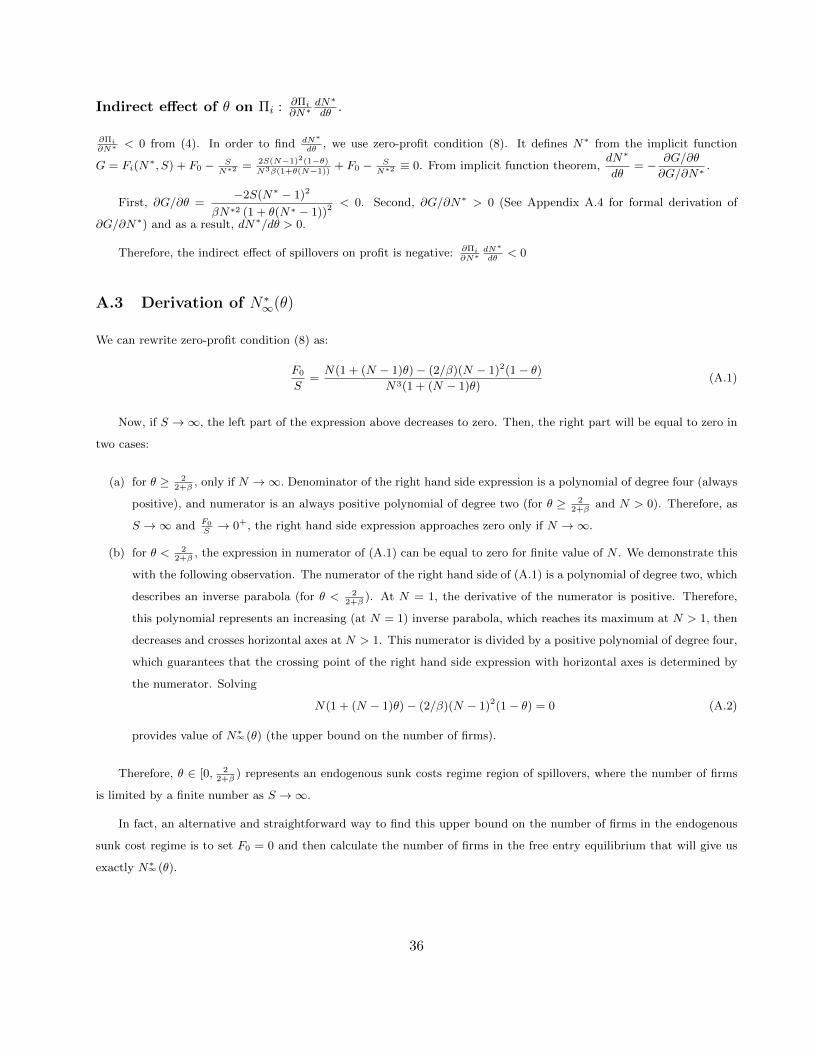
Indirect effect of θ on Πi : ∂Πi∂N∗

dN∗

dθ .

∂Πi∂N∗ < 0 from (4). In order to find dN∗

dθ, we use zero-profit condition (8). It defines N∗ from the implicit function

G = Fi(N∗, S) + F0 − S

N∗2 = 2S(N−1)2(1−θ)N3β(1+θ(N−1))

+ F0 − SN∗2 ≡ 0. From implicit function theorem,

dN∗

dθ= − ∂G/∂θ

∂G/∂N∗.

First, ∂G/∂θ =−2S(N∗ − 1)2

βN∗2 (1 + θ(N∗ − 1))2 < 0. Second, ∂G/∂N∗ > 0 (See Appendix A.4 for formal derivation of

∂G/∂N∗) and as a result, dN∗/dθ > 0.

Therefore, the indirect effect of spillovers on profit is negative: ∂Πi∂N∗

dN∗

dθ< 0

A.3 Derivation of N∗∞(θ)

We can rewrite zero-profit condition (8) as:

F0

S=N(1 + (N − 1)θ)− (2/β)(N − 1)2(1− θ)

N3(1 + (N − 1)θ)(A.1)

Now, if S →∞, the left part of the expression above decreases to zero. Then, the right part will be equal to zero in

two cases:

(a) for θ ≥ 22+β

, only if N →∞. Denominator of the right hand side expression is a polynomial of degree four (always

positive), and numerator is an always positive polynomial of degree two (for θ ≥ 22+β

and N > 0). Therefore, as

S →∞ and F0S→ 0+, the right hand side expression approaches zero only if N →∞.

(b) for θ < 22+β

, the expression in numerator of (A.1) can be equal to zero for finite value of N . We demonstrate this

with the following observation. The numerator of the right hand side of (A.1) is a polynomial of degree two, which

describes an inverse parabola (for θ < 22+β

). At N = 1, the derivative of the numerator is positive. Therefore,

this polynomial represents an increasing (at N = 1) inverse parabola, which reaches its maximum at N > 1, then

decreases and crosses horizontal axes at N > 1. This numerator is divided by a positive polynomial of degree four,

which guarantees that the crossing point of the right hand side expression with horizontal axes is determined by

the numerator. Solving

N(1 + (N − 1)θ)− (2/β)(N − 1)2(1− θ) = 0 (A.2)

provides value of N∗∞(θ) (the upper bound on the number of firms).

Therefore, θ ∈ [0, 22+β

) represents an endogenous sunk costs regime region of spillovers, where the number of firms

is limited by a finite number as S →∞.

In fact, an alternative and straightforward way to find this upper bound on the number of firms in the endogenous

sunk cost regime is to set F0 = 0 and then calculate the number of firms in the free entry equilibrium that will give us

exactly N∗∞(θ).

36

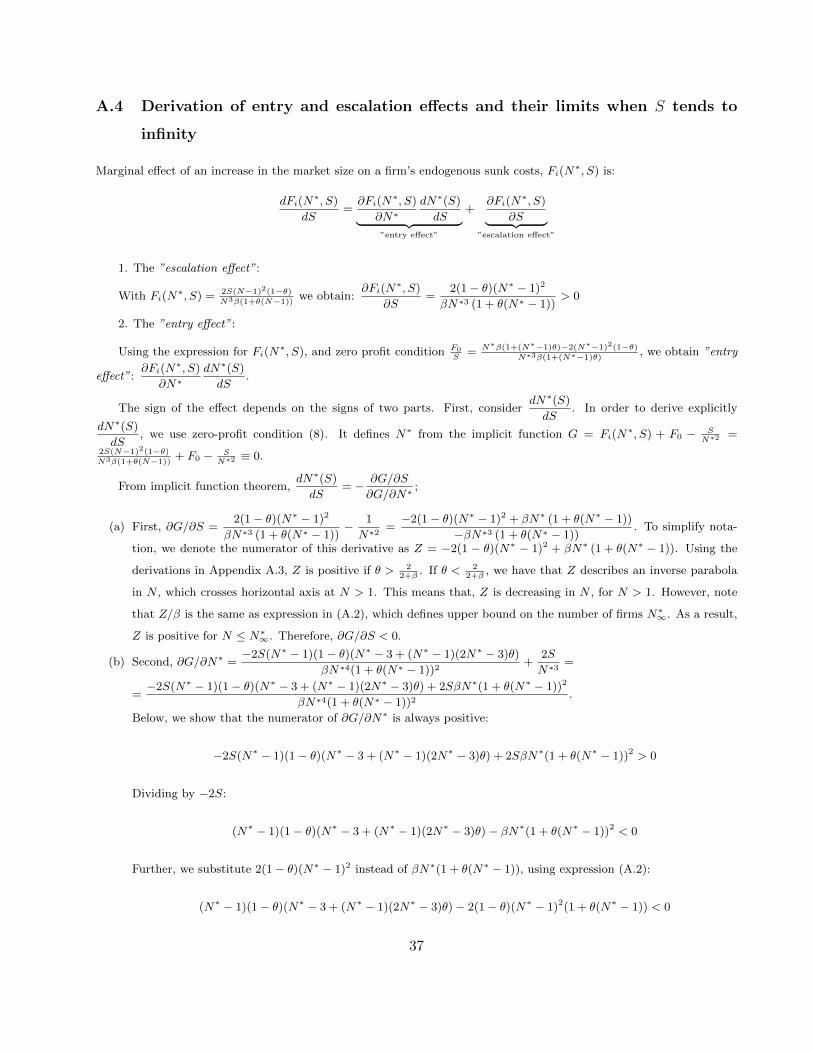
A.4 Derivation of entry and escalation effects and their limits when S tends to

infinity

Marginal effect of an increase in the market size on a firm’s endogenous sunk costs, Fi(N∗, S) is:

dFi(N∗, S)

dS=∂Fi(N

∗, S)

∂N∗dN∗(S)

dS︸ ︷︷ ︸”entry effect”

+∂Fi(N

∗, S)

∂S︸ ︷︷ ︸”escalation effect”

1. The ”escalation effect”:

With Fi(N∗, S) = 2S(N−1)2(1−θ)

N3β(1+θ(N−1))we obtain:

∂Fi(N∗, S)

∂S=

2(1− θ)(N∗ − 1)2

βN∗3 (1 + θ(N∗ − 1))> 0

2. The ”entry effect”:

Using the expression for Fi(N∗, S), and zero profit condition F0

S= N∗β(1+(N∗−1)θ)−2(N∗−1)2(1−θ)

N∗3β(1+(N∗−1)θ), we obtain ”entry

effect”:∂Fi(N

∗, S)

∂N∗dN∗(S)

dS.

The sign of the effect depends on the signs of two parts. First, considerdN∗(S)

dS. In order to derive explicitly

dN∗(S)

dS, we use zero-profit condition (8). It defines N∗ from the implicit function G = Fi(N

∗, S) + F0 − SN∗2 =

2S(N−1)2(1−θ)N3β(1+θ(N−1))

+ F0 − SN∗2 ≡ 0.

From implicit function theorem,dN∗(S)

dS= − ∂G/∂S

∂G/∂N∗;

(a) First, ∂G/∂S =2(1− θ)(N∗ − 1)2

βN∗3 (1 + θ(N∗ − 1))− 1

N∗2=−2(1− θ)(N∗ − 1)2 + βN∗ (1 + θ(N∗ − 1))

−βN∗3 (1 + θ(N∗ − 1)). To simplify nota-

tion, we denote the numerator of this derivative as Z = −2(1 − θ)(N∗ − 1)2 + βN∗ (1 + θ(N∗ − 1)). Using the

derivations in Appendix A.3, Z is positive if θ > 22+β

. If θ < 22+β

, we have that Z describes an inverse parabola

in N , which crosses horizontal axis at N > 1. This means that, Z is decreasing in N , for N > 1. However, note

that Z/β is the same as expression in (A.2), which defines upper bound on the number of firms N∗∞. As a result,

Z is positive for N ≤ N∗∞. Therefore, ∂G/∂S < 0.

(b) Second, ∂G/∂N∗ =−2S(N∗ − 1)(1− θ)(N∗ − 3 + (N∗ − 1)(2N∗ − 3)θ)

βN∗4(1 + θ(N∗ − 1))2+

2S

N∗3=

=−2S(N∗ − 1)(1− θ)(N∗ − 3 + (N∗ − 1)(2N∗ − 3)θ) + 2SβN∗(1 + θ(N∗ − 1))2

βN∗4(1 + θ(N∗ − 1))2.

Below, we show that the numerator of ∂G/∂N∗ is always positive:

−2S(N∗ − 1)(1− θ)(N∗ − 3 + (N∗ − 1)(2N∗ − 3)θ) + 2SβN∗(1 + θ(N∗ − 1))2 > 0

Dividing by −2S:

(N∗ − 1)(1− θ)(N∗ − 3 + (N∗ − 1)(2N∗ − 3)θ)− βN∗(1 + θ(N∗ − 1))2 < 0

Further, we substitute 2(1− θ)(N∗ − 1)2 instead of βN∗(1 + θ(N∗ − 1)), using expression (A.2):

(N∗ − 1)(1− θ)(N∗ − 3 + (N∗ − 1)(2N∗ − 3)θ)− 2(1− θ)(N∗ − 1)2(1 + θ(N∗ − 1)) < 0

37

Dividing by (N∗ − 1)(1− θ):

(N∗ − 3 + (N∗ − 1)(2N∗ − 3)θ)− 2(N∗ − 1)(1 + θ(N∗ − 1)) < 0

N∗ − 3 + (N∗ − 1)(2N∗ − 3)θ < 2(N∗ − 1)(1 + θ(N∗ − 1))

Opening the brackets:

N∗ − 3 + 2N∗2θ − 5N∗θ + 3θ < −2 + 2N∗ + 2θ − 4N∗θ + 2N∗2θ

and simplifying, we obtain

−1 + θ < N∗(1 + θ)

which always holds. Therefore, ∂G/∂N∗ > 0.

As a result, we have that dN∗/dS > 0.

Now, we consider the first part of ”entry effect”:∂Fi(N

∗, S)

∂N∗. Typically, as the number of firms increases, each firm

has fewer incentives to invest into quality:∂Fi(N

∗, S)

∂N∗< 0. In our setup this is also the case unless spillovers are zero

or rather small.

∂Fi(N∗, S)

∂N∗=−2S(N∗ − 1)(1− θ)(N∗ − 3 + (N∗ − 1)(2N∗ − 3)θ)

βN∗4(1 + θ(N∗ − 1))2. The sign of this derivative depends on the sign

of N∗ − 3 + (N∗ − 1)(2N∗ − 3)θ. For θ > θc, where θc = 3−N∗(N∗−1)(2N∗−3)

, we have that N∗ − 3 + (N∗ − 1)(2N∗ − 3)θ > 0

and∂Fi(N

∗, S)

∂N∗< 0. On the other hand, for θ < θc, we have that

∂Fi(N∗, S)

∂N∗> 0

Vives (2008) assigns the general ambiguity of the sign of∂Fi(N

∗, S)

∂N∗to the two opposing effects: i) the direct demand

(or size) effect, and ii) the indirect (or elasticity) price pressure effects. The direct demand effect predicts that, for a

given market size, if more firms enter, the residual demand of a firm will decline, and a firm has less incentives to invest

in R&D. The elasticity of residual demand however will increase, and this will have positive effect of the R&D incentives

because with higher elasticity of demand (that a firm faces) it is optimal for a firm to expand output and that, in turn,

makes the investment in R&D more attractive. The latter describes the second, indirect price pressure (elasticity) effect.

Note that the direct demand effect typically dominates the price pressure effect, and R&D decreases with the number of

firms. However, as we have just seen, it is possible that under certain circumstances (zero or very small spillovers in our

case) it is the other way around (see Vives, 2008, for a comprehensive discussion on this point).

As already noted, this ”entry effect” ∂Fi(N∗,S)

∂N∗ × dN∗

dSis of second order importance for large market. Thus, the

direct ”escalation effect” ∂Fi(N∗,S)

∂Sdominates, and governs the effect of S on endogenous sunk costs. In our setup, the

”entry effect” turns out to be:

∂Fi(N∗, S)

∂N∗× dN∗

dS=

=F0

S

(N∗ − 1)(θ − 1)(N∗ − 3 + 1(N∗ − 1)(2N∗ − 3)θ)

(N∗(4−N∗ + β) + 6θ − 3− 2N∗(6 +N∗2 + β −N∗(4 + β))θ + (N∗ − 1)2(N∗(2 + β)− 3)θ2(A.3)

38

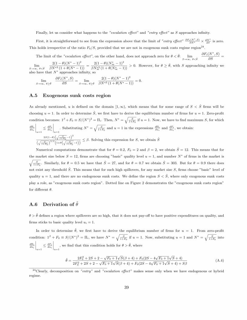
Finally, let us consider what happens to the ”escalation effect” and ”entry effect” as S approaches infinity.

First, it is straightforward to see from the expression above that the limit of ”entry effect” ∂Fi(N∗,S)

∂N∗ × dN∗

dSis zero.

This holds irrespective of the ratio F0/S, provided that we are not in exogenous sunk costs regime region24.

The limit of the ”escalation effect”, on the other hand, does not approach zero for θ < θ: limS→∞, θ<θ

∂Fi(N∗, S)

∂S=

limS→∞, θ<θ

2(1− θ)(N∗ − 1)2

βN∗3 (1 + θ(N∗ − 1))=

2(1− θ)(N∗∞ − 1)2

βN∗3∞ (1 + θ(N∗∞ − 1))> 0. However, for θ ≥ θ, with S approaching infinity we

also have that N∗ approaches infinity, so

limS→∞, θ≥θ

∂Fi(N∗, S)

∂S= limS→∞, θ≥θ

2(1− θ)(N∗ − 1)2

βN∗3 (1 + θ(N∗ − 1))= 0.

A.5 Exogenous sunk costs region

As already mentioned, u is defined on the domain [1,∞), which means that for some range of S < S firms will be

choosing u = 1. In order to determine S, we first have to derive the equilibrium number of firms for u = 1. Zero-profit

condition becomes: 1β +F0 ≡ S/(N∗)2 = Πi. Then, N∗ =√

S1+F0

if u = 1. Now, we have to find maximum S, for which

dΠidui

∣∣∣∣u=1

≤ dFidui

∣∣∣∣u=1

. Substituting N∗ =√

S1+F0

and u = 1 in the expressions dΠidui

and dFidui

, we obtain:

2S(1−θ)(√

S1+F0

−1)2

(√S

1+F0

)3/2(1+θ

(√S

1+F0−1)) ≤ β. Solving this expression for S, we obtain S

Numerical computations demonstrate that for θ = 0.2, F0 = 2 and β = 2, we obtain S = 12. This means that for

the market size below S = 12, firms are choosing ”basic” quality level u = 1, and number N∗ of firms in the market is√S

1+F0. Similarly, for θ = 0.5 we have that S = 27, and for θ = 0.7 we obtain S = 303. But for θ = 0.9 there does

not exist any threshold S. This means that for such high spillovers, for any market size S, firms choose ”basic” level of

quality u = 1, and there are no endogenous sunk costs. We define the region S < S, where only exogenous sunk costs

play a role, as ”exogenous sunk costs region”. Dotted line on Figure 2 demonstrates the ”exogenous sunk costs region”

for different θ.

A.6 Derivation of θ

θ > θ defines a region where spillovers are so high, that it does not pay-off to have positive expenditures on quality, and

firms sticks to basic quality level ui = 1.

In order to determine θ, we first have to derive the equilibrium number of firms for u = 1. From zero-profit

condition: 1β + F0 ≡ S/(N∗)2 = Πi, we have N∗ =√

S1+F0

if u = 1. Now, substituting u = 1 and N∗ =√

S1+F0

into

dΠidui

∣∣∣∣u=1

≤ dFidui

∣∣∣∣u=1

, we find that this condition holds for θ > θ, where

θ =2F 2

0 + 2S + 2−√F0 + 1

√S(β + 4) + F0(2S − 4

√F0 + 1

√S + 4)

2F 20 + 2S + 2−

√F0 + 1

√S(β + 4) + F0(2S − 4

√F0 + 1

√S + 4) + Sβ

(A.4)

24Clearly, decomposition on ”entry” and ”escalation effect” makes sense only when we have endogenous or hybridregime.

39

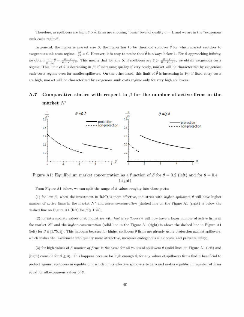
Therefore, as spillovers are high, θ > θ, firms are choosing ”basic” level of quality u = 1, and we are in the ”exogenous

sunk costs regime”.

In general, the higher is market size S, the higher has to be threshold spillover θ for which market switches to

exogenous sunk costs regime: dθdS

> 0. However, it is easy to notice that θ is always below 1. For S approaching infinity,

we obtain limS→∞

θ = 2(1+F0)2(1+F0)+β

. This means that for any S, if spillovers are θ > 2(1+F0)2(1+F0)+β

, we obtain exogenous costs

regime. This limit of θ is decreasing in β: if increasing quality if very costly, market will be characterized by exogenous

sunk costs regime even for smaller spillovers. On the other hand, this limit of θ is increasing in F0: if fixed entry costs

are high, market will be characterized by exogenous sunk costs regime only for very high spillovers.

A.7 Comparative statics with respect to β for the number of active firms in the

market N∗

Figure A1: Equilibrium market concentration as a function of β for θ = 0.2 (left) and for θ = 0.4(right)

From Figure A1 below, we can split the range of β values roughly into three parts:

(1) for low β, when the investment in R&D is more effective, industries with higher spillovers θ will have higher

number of active firms in the market N∗ and lower concentration (dashed line on the Figure A1 (right) is below the

dashed line on Figure A1 (left) for β ≤ 1.75);

(2) for intermediate values of β, industries with higher spillovers θ will now have a lower number of active firms in

the market N∗ and the higher concentration (solid line in the Figure A1 (right) is above the dashed line in Figure A1

(left) for β ∈ [1.75, 3]). This happens because for higher spillovers θ firms are already using protection against spillovers,

which makes the investment into quality more attractive, increases endogenous sunk costs, and prevents entry;

(3) for high values of β number of firms is the same for all values of spillovers θ (solid lines on Figure A1 (left) and

(right) coincide for β ≥ 3). This happens because for high enough β, for any values of spillovers firms find it beneficial to

protect against spillovers in equilibrium, which limits effective spillovers to zero and makes equilibrium number of firms

equal for all exogenous values of θ.

40

References

Amir, R. (2000). Modelling imperfectly appropriable R&D via spillovers. International Journal of

Industrial Organization 18 (7), 1013–1032.

Amir, R., I. V. Evstigneev, and J. Wooders (2003). Noncooperative versus cooperative R&D with

endogenous spillover rates. Games and Economic Behavior 42 (2), 183–207.

Anton, J. J., H. Greene, and D. A. Yao (2006). Policy implications of weak patent rights. Innovation

Policy and the Economy 6, 1.

Arundel, A. (2001). The relative effectiveness of patents and secrecy for appropriation. Research

policy 30 (4), 611–624.

Aschhoff, B., E. Baier, D. Crass, M. Hud, P. Hunermund, C. Kohler, B. Peters, C. Rammer,

E. Schricke, T. Schubert, and F. Schwiebacher (2013). Innovation in Germany - results of the

German CIS 2006 to 2010. Background report on the Innovation Surveys 2007, 2009 and 2011 of

the Mannheim Innovation Panel. ZEW Dokumentationen 13-01, ZEW - Zentrum fur Europaische

Wirtschaftsforschung / Center for European Economic Research.

Atallah, G. (2004). The protection of innovations. Cirano working papers, CIRANO.

Behringer, S. (2014). Network effects, spillovers and market structure. The Manchester School 82 (2),

143–159.

Berry, S. and J. Waldfogel (2010). Product quality and market size. The Journal of Industrial

Economics 58 (1), 1–31.

Bloom, N., M. Schankerman, and J. Van Reenen (2013). Identifying technology spillovers and product

market rivalry. Econometrica 81 (4), 1347–1393.

Bresnahan, T. F. (1992). Sutton’s sunk costs and market structure: Price competition, advertising,

and the evolution of concentration.

Bronnenberg, B. J., S. K. Dhar, and J.-P. Dube (2005). Endogenous sunk costs and the geographic

distribution of brand shares in consumer package goods industries. Technical report, Citeseer.

41

Carlton, D. W. (2005, Oct). Barriers To Entry. NBER Working Papers 11645, National Bureau of

Economic Research, Inc.

Cohen, W. M., A. Goto, A. Nagata, R. R. Nelson, and J. P. Walsh (2002). R&D spillovers, patents

and the incentives to innovate in Japan and the United States. Research Policy 31 (8), 1349–1367.

Cohen, W. M. and R. C. Levin (1989). Empirical studies of innovation and market structure. In

R. Schmalensee and R. Willig (Eds.), Handbook of Industrial Organization (1 ed.), Volume 2, Chap-

ter 18, pp. 1059–1107. Elsevier.

Cohen, W. M. and D. A. Levinthal (1989). Innovation and learning: The two faces of R&D. The

Economic Journal 99 (397), pp. 569–596.

Cohen, W. M., R. R. Nelson, and J. P. Walsh (2000). Protecting their intellectual assets: Appro-

priability conditions and why us manufacturing firms patent (or not). Technical report, National

Bureau of Economic Research.

Coscolla-Girona, P., P. Beneito, A. Sanchis Llopis, and M. E. Rochina Barrachina (2011). Competitive

pressure determinants and innovation at the firm level. Technical report, Instituto Valenciano de

Investigaciones Economicas, SA (Ivie).

d’Aspremont, C. and A. Jacquemin (1988). Cooperative and noncooperative R&D in duopoly with

spillovers. American Economic Review 78 (5), 1133–37.

De Bondt, R. (1997). Spillovers and innovative activities. International Journal of Industrial Organi-

zation 15 (1), 1–28.

Dick, A. A. (2007). Market size, service quality, and competition in banking. Journal of Money, Credit

and Banking 39 (1), 49–81.

Ellickson, P. B. (2007). Does Sutton apply to supermarkets? The RAND Journal of Economics 38 (1),

43–59.

Etro, F. (2013). Some thoughts on the Sutton approach. Journal of Economics, 1–15.

Gersbach, H. and A. Schmutzler (2003). Endogenous spillovers and incentives to innovate. Economic

Theory 21 (1), 59–79.

42

Hall, B., C. Helmers, M. Rogers, and V. Sena (2014). The choice between formal and informal

intellectual property: A review. Journal of Economic Literature 52 (2), 1–50.

Hall, B. H., J. Mairesse, and P. Mohnen (2010). Chapter 24 - Measuring the returns to R&D. In B. H.

Hall and N. Rosenberg (Eds.), Handbook of the Economics of Innovation, Volume 2, Volume 2 of

Handbook of the Economics of Innovation, pp. 1033 – 1082. North-Holland.

Hanel, P. and A. St-Pierre (2002). Effects of R&D spillovers on the profitability of firms. Review of

Industrial Organization 20 (4), 305–322.

Henry, E. and F. Ruiz-Aliseda (2012). Innovation beyond patents: Technological complexity as a

protection against imitation. Technical report, CEPR Discussion Papers.

Hinloopen, J. (2000, October). More on subsidizing cooperative and noncooperative R&D in duopoly

with spillovers. Journal of Economics 72 (3), 295–308.

Kamien, M., E. Muller, and I. Zang (1992). Research joint ventures and R&D cartels. American

Economic Review 82 (5), 1293–306.

Keller, W. (2004). International technology diffusion. Journal of economic literature, 752–782.

Koski, H. and T. Kretschmer (2010). New product development and firm value in mobile handset

production. Information Economics and Policy 22 (1), 42–50.

Kunin, M., J. Strelicky, and K. Zigic (2013). The interaction between private and public ipr protection

in a software market: A positive and normative analysis. CERGE-EI Working Paper Series (490).

Leiponen, A. and J. Byma (2009). If you cannot block, you better run: Small firms, cooperative

innovation, and appropriation strategies. Research Policy 38 (9), 1478–1488.

Mansfield, E. (1984). R&D and innovation: some empirical findings. In Z. Griliches (Ed.), R&D,

Patents, and Productivity, NBER Chapters, pp. 127–154. National Bureau of Economic Research,

Inc.

Mansfield, E. (1986). Patents and innovation: an empirical study. Management science 32 (2), 173–181.

Mansfield, E., M. Schwartz, and S. Wagner (1981). Imitation costs and patents: an empirical study.

Economic Journal 91 (364), 907–18.

43

Matraves, C. (1999). Market structure, R&D and advertising in the pharmaceutical industry. Journal

of Industrial Economics 47 (2), 169–94.

Matraves, C. and L. Rondi (2005). Product differentiation, turbulence and sustainability of competitive

advantage. Technical report, working paper, March.

Nocke, V. (2007). Collusion and dynamic (under-) investment in quality. The RAND Journal of

Economics 38 (1), 227–249.

Poyago-Theotoky, J. (1999). A note on endogenous spillovers in a non-tournament R&D duopoly.

Review of Industrial Organization 15 (3), 253–262.

Robinson, W. T. and J. Chiang (1996). Are ’s predictions robust?: Empirical insights into advertising,

R&D, and concentration. The Journal of Industrial Economics, 389–408.

Samuelson, P. and S. Scotchmer (2002). The law and economics of reverse engineering. Yale Law

Journal , 1575–1663.

Schmalensee, R. (1992). Sunk costs and market structure: A review article. The Journal of Industrial

Economics, 125–134.

Scotchmer, S. (2006). Innovation and Incentives (1 ed.), Volume 1. The MIT Press.

Senyuta, O. and K. Zigic (2012). Managing spillovers: an endogenous sunk cost approach. Economics

Institute, Academy of Sciences of the Czech Republic.

Shenkar, O. (2010). Copycats: How Smart Companies Use Imitation to Gain a Strategic Edge.

McGraw-Hill Education.

Spence, A. M. (1984). Cost reduction, competition, and industry performance. Econometrica 52 (1),

101–21.

Strelicky, J. and K. Zigic (2011). Intellectual property rights protection and enforcement in a software

duopoly. CERGE-EI Working Paper Series (435).

Sutton, J. (1991). Sunk Costs and Market Structure: Price Competition, Advertising, and the Evolution

of Concentration. The MIT Press.

44

Sutton, J. (2001). Technology and Market Structure: Theory and History (1 ed.), Volume 1. The MIT

Press.

Sutton, J. (2007). Market structure: Theory and evidence. In M. Armstrong and R. Porter (Eds.),

Handbook of Industrial Organization, Volume 3, Chapter 35, pp. 2301–2368. Elsevier.

Suzumura, K. (1992). Cooperative and noncooperative R&D in an oligopoly with spillovers. American

Economic Review 82 (5), 1307–20.

Taylor, M. S. (1993). Trips, trade, and technology transfer. The Canadian Journal of Economics 26 (3),

625–637.

Tesoriere, A. (2008). A further note on endogenous spillovers in a non-tournament R&D duopoly.

Review of Industrial Organization 33 (2), 177–184.

Vasconcelos, H. (2006). Endogenous mergers in endogenous sunk cost industries. International Journal

of Industrial Organization 24 (2), 227–250.

Vives, X. (2008). Innovation and competitive pressure. Journal of Industrial Economics 56 (3), 419–

469.

Zabojnik, J. (2002). A theory of trade secrets in firms. International Economic Review 43 (3), 831–855.

45