Managing financial risk in planning under uncertainty - ResearchGate

Managing Financial Risk in Planningunder Uncertainty

Andres Barbaro and Miguel J. BagajewiczSchool of Chemical Engineering and Materials Science, University of Oklahoma, Norman, OK 73019

DOI 10.1002/aic.10094Published online in Wiley InterScience (www.interscience.wiley.com).

A methodology is presented to include financial risk management in the framework oftwo-stage stochastic programming for planning under uncertainty. A known probabilisticdefinition of financial risk is adapted to be used in this framework and its relation todownside risk is analyzed. Using these definitions, new two-stage stochastic programmingmodels that manage financial risk are presented. Computational issues related to thesemodels are also discussed. © 2004 American Institute of Chemical Engineers AIChE J, 50:963–989, 2004Keywords: planning, financial risk, robust optimization

Introduction

Planning under uncertainty is a common class of problemsfound in process systems engineering. Some examples widelyfound in the literature are capacity expansion, scheduling,supply chain management, resource allocation, transportation,unit commitment, and product design problems. The first stud-ies on planning under uncertainty could be accredited toDantzig (1955) and Beale (1955), who proposed the two-stagestochastic models with recourse, which provide the mathemat-ical framework for this article.

The industrial importance of planning process capacity ex-pansions under uncertainty has been widely recognized anddiscussed by several researchers (Ahmed and Sahinidis, 2000b;Berman and Ganz, 1994; Eppen et al., 1989; Liu and Sahinidis,1996; Murphy et al., 1987; Sahinidis et al., 1989). In themajority of industrial applications, capacity expansion plansrequire considerable amount of capital investment over a long-range time horizon. Moreover, the inherent level of uncertaintyin forecast demands, availabilities, prices, technology, capital,markets, and competition make these decisions very challeng-ing and complex. Therefore, several approaches were proposedto formulate and solve this problem. They mainly differ in theway uncertainty is handled, the robustness of the plans, and

their flexibility. This article follows the two-stage stochasticprogramming approach with discretization of the uncertaintyspace by random sampling of the parameter probability distri-butions. In turn, the feasibility constraints for the problem areenforced for every scenario in a deterministic fashion (takingrecourse actions with an associated cost) such that the resultingplan or design is feasible under every possible uncertaintyrealization.

A formal two-stage stochastic model for capacity planning inthe process industry was presented by Liu and Sahinidis (1996)as an extension of the deterministic models developed bySahinidis et al. (1989). In the two-stage stochastic approach, itis assumed that the capacity expansion plan is decided beforethe actual realization of uncertain parameters (scenarios), al-lowing only some operational recourse actions to take place toimprove the objective and correct any infeasibility. In thisformulation, the objective is usually to maximize the expectedprofit or to minimize the expected cost over the two stages ofthe capacity expansion project. Typically, the resulting objec-tive function is accounted using the expected net present valueor ENPV. In addition to the two-stage optimization, otherapproaches have been proposed to deal with uncertainties in themodel parameters such as chance-constrained optimization(Charnes and Cooper, 1959), fuzzy programming (Bellman andZadeh, 1970; Zimmermann, 1987), and the design flexibilityapproach (Ierapetritou and Pistikopoulos, 1994).

In the chance-constrained approach, some of the problemconstraints are expressed in terms of probabilistic statements,

Correspondence concerning this article should be addressed to M. J. Bagajewicz [email protected].

© 2004 American Institute of Chemical Engineers

PROCESS SYSTEMS ENGINEERING

AIChE Journal 963May 2004 Vol. 50, No. 5

typically requiring that they be satisfied with a probabilitygreater than a desired level. This approach is particularly usefulwhen the cost and benefits of second-stage decisions are diffi-cult to assess because the use of second-stage or recourseactions is avoided.

In turn, fuzzy programming assumes that the uncertain pa-rameters can be represented by fuzzy numbers, whereas con-straints are considered fuzzy sets. This approach also allowssome constraint violation and their degree of satisfaction isdefined as the membership function of the constraint. A com-parison of fuzzy and two-stage stochastic programming madeby Liu and Sahinidis (1996), in the context of capacity plan-ning problems, showed that the latter offers several advantagesover the former.

Finally, Ierapetritou and Pistikopoulos (1994) proposed anapproach in which the plan or design is feasible only inside acertain region of the uncertainty space rather than for allpossible uncertainty realizations. Then, a flexibility index isused to measure the extent of the plan’s feasible uncertaintyregion. In the cited article, the authors used a flexibility indexthat represents the largest hypercube that can be inscribedinside the plan’s feasible uncertainty region. In this approach,however, it is difficult to assess the trade-off between cost andflexibility.

A major limitation of all the mentioned approaches is thatthey consider, in one way or another, “expected outcomes” ofthe problem objective without explicitly taking into account itsvariability. Specifically, the two-stage stochastic models do nottake into account the variability of the second-stage cost orprofit but only its expected value. This was first discussed byEppen et al (1989) in their work on automotive industry ca-pacity planning. They proposed to use the concept of downsiderisk to measure the recourse cost variability and obtain solu-tions appealing to a risk-averse investor. Another approach todeal with the second-stage cost variability was proposed byMulvey et al. (1995), who introduced the concept of robustnessas the property of a solution for which the objective value forany realized scenario remains “close” to the expected objectivevalue over all possible scenarios. Originally, the models forrobust planning under uncertainty presented by Mulvey et al.(1995) used the variance of the cost as a “measure” of therobustness of the plan: that is, less variance corresponds tohigher robustness. More recently, Ahmed and Sahinidis (1998),aiming at eliminating the nonlinearities introduced by the vari-ance, proposed the use of the upper partial mean (UPM) as ameasure of the variability of the recourse costs. They also offera complete literature review on the problem. In addition to itslinearity, the main advantage of using the UPM, as opposed tothe variance, is its asymmetric nature that penalizes only theunfavorable cases from a risk perspective. However, the UPMsuffers from limitations that make it an inappropriate measureto assess and manage financial risk. Because of the way theUPM is defined, a solution may falsely reduce its variabilityjust by not choosing optimal second-stage decisions. Makingnonoptimal second-stage decisions reduces the expected profit,allowing the positive deviation between the expected second-stage profit and the profit for that scenario (�s) to be zero forsome scenarios that otherwise would have a profit lower thanthe actual expected value and therefore �s greater than zero.Because nobody would want to obtain a lower profit when ahigher value is already attainable, operating with nonoptimal

second-stage policies does not make sense from a financialpoint of view. This is discussed in detail by Takriti and Ahmed(2003), who present sufficient conditions for the variabilitymeasure of a robust optimization to ensure that the solutionsare optimal in profit.

A different perspective to evaluate risk is also presented inthe work of Ierapetritou and Pistikopoulos (1994). In thatarticle, the authors proposed to use regret functions as anindirect measure of financial risk. For any realization of uncer-tain parameters, the regret function measures the differencebetween the objective function resulting from the actual plan ordesign, and the plan that is optimal for that realization ofuncertain parameters. Then, the idea is to find plans that havelow regret for the set of feasible uncertain parameters. Thisapproach has two major difficulties. First, financial risk isevaluated only indirectly because the regret functions measureonly the potential losses of the actual plan in comparison witha hypothetical plan that is optimal for only a specific uncer-tainty realization (no information is given about the feasibilityof that plan under other circumstances). Thus, the regret func-tions do not provide any information about the financial risk.The second disadvantage of this approach is that to constructeach regret function a separate optimization problem has to besolved for each possible uncertainty realization, which greatlyincreases the computational complexity of the problems.

Another approach, recently suggested by Cheng et al.(2003), is to rely on a Markov decision process modeling thedesign/production decisions at each epoch of the process as atwo-stage stochastic program. The Markov decision processused is similar in nature to a multistage stochastic program-ming where structural decisions are also considered as possiblerecourse actions. Their solution procedure relies on dynamicprogramming techniques and is applicable only if the problemsare separable and monotone. In addition, they propose to departfrom single-objective paradigms, and use a multiobjective ap-proach, rightfully claiming that cost is not necessarily the onlyobjective and that other objectives are usually also important,like social consequences, environmental impact, and processsustainability, for example. Among these other objectives, theyinclude risk (measured by downside risk, as introduced byEppen et al., 1989), which under the assumption that decisionmakers are risk-averse, they claim should be minimized.

Aside from the fact that some level of risk could be tolerableat low profit aspirations to achieve larger gains at higher ones,thus promoting a risk-taking attitude, this assumption has someimportant additional limitations. As it will become apparentlater in this article, given that downside risk is a function notonly of the first-stage decisions but also of the aspiration ortarget profit level, minimizing downside risk at one level doesnot imply its minimization at another. Moreover, minimizingdownside risk does not necessarily lead to minimizing financialrisk for the specified target, a result that is discussed later inthis article. Thus, treating financial risk as a single objectivepresents some limitations, and we propose that risk be managedover the entire range of aspiration levels. Applequist et al.(2000) proposed to manage risk at the design stages by usingthe concept of risk premium. They observed that for a varietyof investments, the rate of return correlates linearly with thevariability, which leads to the definition risk premium. Basedon this observation, they suggest benchmarking new investmentsagainst the historical risk premium mark. Thus, they propose a

964 AIChE JournalMay 2004 Vol. 50, No. 5

two-objective problem, where the expected net present valueand the risk premium are both maximized. The technique relieson using the variance as a measure of variability and thereforeit penalizes scenarios at both sides of the mean equally, whichis the same limitation discussed above. Recently, Gupta andMaranas (2003), while analyzing risk, also realized that sym-metric measures were disadvantageous and therefore proposedto use a function very similar to the one we discuss in thisarticle, but due to computational problems they resort to max-imize the worst case scenario outcome. We point out that theirdefinition of risk similar to the one proposed earlier by Barbaroand Bagajewicz (2003) have been used previously to assess(but not manage) risk, one of the most notorious examplesbeing the petroleum exploration and production field (McCray,1975).

The main objective of this article is to develop new mathe-matical formulations for problems dealing with planning anddesign under uncertainty that allow management of financialrisk according to the decision maker’s preference. A major steptoward this objective is the use of a formal probabilistic defi-nition of financial risk. In addition to this, the connectionbetween downside risk, first introduced by Eppen et al. (1989),and financial risk is discussed. Using these two definitions, newtwo-stage stochastic programming models that are able tomanage financial risk are developed. The advantages of theproposed approaches are that they maintain the original MILPstructure of the problem. The theory developed in this article isof general application to any planning and design under uncer-tainty problem that can be formulated using a two-stage sto-chastic formulation.

The article is organized as follows. The “Two-Stage Sto-chastic Programming” section reviews general aspects of thetwo-stage stochastic formulation for planning under uncer-tainty. A theoretical definition of financial risk is introduced inthe “Financial Risk Management” section, and the “DownsideRisk: An Advantageous Measure to Assess and Manage Finan-cial Risk” and “Other Measure of Risk: Value at Risk and RiskAdjusted Project Value” sections explore the connection be-tween this definition and other risk measures. The “Two-StageStochastic Programming with Financial Risk Constraints” and“Two-Stage Stochastic Programming Using Downside Risk”sections outline new two-stage stochastic programming modelsto manage financial risk that are then applied to an illustrativeprocess planning problem in the “Illustrative Example” section.Finally, “Computational Issues for Large-Scale Problems Us-ing Model RO-SP-DR” discusses some issues related to thecomputational performance of the proposed formulations.

Two-Stage Stochastic Programming

This kind of optimization problems is characterized by twoessential features: the uncertainty in the problem data and thesequence of decisions. Some of the model parameters areconsidered random variables with a certain probability distri-bution. In turn, some decisions are taken at the planning stage,that is, before the uncertainty is revealed, whereas a number ofother decisions can be made only after the uncertain databecome known. The first class of decisions is called the first-stage decisions, and the period when these decisions are takenis referred to as the first stage. On the other hand, the decisionsmade after the uncertainty is unveiled are called second-stage

or recourse decisions and the corresponding period is called thesecond stage. Typically, first-stage decisions are structural andmost of the time related to capital investment at the beginningof the project, whereas the second-stage decisions are oftenoperational. Yet, some structural decisions corresponding to afuture time can be considered as a second stage, that is, onemay want to wait until some uncertainty (not necessarily all) isrealized to make additional structural decisions. This kind ofsituations is formulated through the so-called multistage mod-els, which are a natural extension of the two-stage case. Amongthe two-stage stochastic models, the expected value of the cost(or profit) resulting from optimally adapting the plan accordingto the realizations of uncertain parameters is referred to as therecourse function. Thus, a problem is said to have completerecourse if the recourse cost (or profit) for every possibleuncertainty realization remains finite, independently of thenature of the first-stage decisions. In turn, if this statement istrue only for the set of feasible first-stage decisions, the prob-lem is said to have relatively complete recourse (Birge andLouveaux, 1997). This condition means that for every feasiblefirst-stage decision, there is a way of adapting the plan to therealization of uncertain parameters. Another important prop-erty of certain two-stage problems, referred to as fixed re-course, will be discussed later. These properties are highlydesirable and are found in most practical applications of thiskind of optimization problems.

A large and useful collection of literature exists on two-stagestochastic programming modeling and solution techniques.Some excellent references are the books by Infanger (1994),Kall and Wallace (1994), Higle and Sen (1996), Birge andLouveaux (1997), Marti and Kall (1998), and Uryasev andPardalos (2001). In addition, the articles by Pistikopoulos andIerapetritou (1995), Cheung and Powell (1995), Iyer andGrossmann (1998), and Verweij et al. (2003) provide verygood references on solution techniques for these problems.

The general extensive form of a two-stage mixed-integerlinear stochastic problem for a finite number of scenarios canbe written as follows (Birge and Louveaux, 1997).

Model SP

Max E�Profit� � �s�S

psqsTys � cTx (1)

s.t.

Ax � b (2)

Tsx � Wys � hs � s � S (3)

x � 0 x � X (4)

ys � 0 � s � S (5)

In the above model, x represents the first-stage mixed-integerdecision variables and ys are the second-stage variables corre-sponding to scenario s, which has occurrence probability ps.The objective function is composed of the expectation of theprofit generated from operations minus the cost of first-stage


decisions (capital investment). The uncertain parameters in thismodel appear in the coefficients qs, the technology matrix Ts,and in the independent term hs. In this article, the study wasrestricted to the cases where W, the recourse matrix, is deter-ministic. This is referred to in the literature as a problem withfixed recourse and ensures that the second-stage feasible regionis convex and closed, and that the recourse function is apiecewise linear convex function in x (Birge and Louveaux,1997). Cases where W is not fixed are found for instance inportfolio optimization when the interest rates are uncertain(Dupacova and Romisch, 1998). The above formulation con-siders the maximization of profit as an objective function butthe same concepts and analysis developed in this article arevalid for the case where the objective is the minimization ofcost.

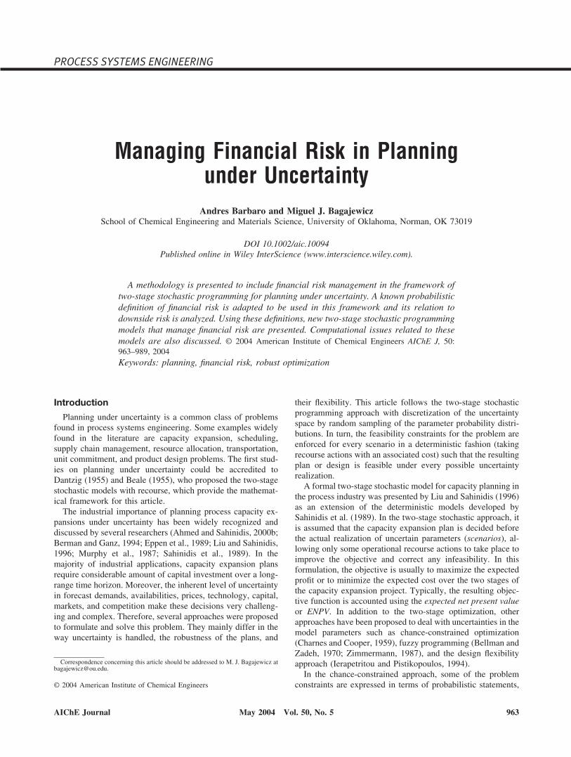
When trying to analyze the usefulness of model SP in thecontext of risk management one first notices that, even thoughit maximizes the total expected profit, it does not provide anycontrol over the variability of the profit over the differentscenarios. For instance, consider the profit histogram of twogeneric feasible solutions shown in Figure 1. The first designhas a higher expected profit (M$ 3.38) than the second one (M$3.35); however, Design I is riskier than Design II becausefinancial loss can occur under several scenarios. On the otherhand, Design II renders positive profits for all scenarios.

Thus, a risk-averse investor would prefer Design II becauseit gives almost the same expected profit level and exhibitslower financial risk. This kind of preferences cannot be cap-tured using model SP, because it does not contain any infor-mation about the variability of the profit. Then, a proper mea-sure of financial risk needs to be included in the formulation toallow the decision maker to obtain solutions according tohis/her desired risk exposure level.

Financial Risk Management

This section introduces several theoretical aspects for riskmanagement. A formal definition of financial risk in the frame-work of two-stage stochastic programming is first introducedand then analyzed in terms of the profit probability distribution.

This is the core of the risk management strategies that will bepresented later in this article.

Probabilistic definition of financial risk

Financial risk associated with a planning project can bedefined as the probability of not meeting a certain target profit(maximization) or cost (minimization) level referred to as �.For the two-stage stochastic problem (SP), the financial riskassociated with a design x and a target profit � is thereforeexpressed by the following probability

Risk�x, �� P�Profit�x� � �� (6)

where Profit(x) is the actual profit, that is, the profit resultingafter the uncertainty has been unveiled and a scenario realized.As stated above, this definition has been made before (McCray,1975). For instance, if one revisits the examples shown inFigure 1, one can see there is a 12% probability that Design Idoes not make a positive profit (� � 0). Similarly, Design IIhas no risk of yielding negative profits, that is, Risk(Design II,0) � 0.

To obtain an explicit expression for financial risk, let theprofit corresponding to the realization of each scenario be

Profits�x� � qsTys � cTx � s � S (7)

where ys is the optimal second-stage solution for scenario s.Because uncertainty in the two-stage formulation is representedthrough a finite number of independent and mutually exclusivescenarios, the above probability can be expressed in terms ofthe probability of not meeting the target profit in each individ-ual scenario realization

Risk�x, �� s�S

P�Profits�x� � �� s�S

P�qsTys � cTx � ��

(8)

Furthermore, for a given design the probability of not meet-ing the target profit in each particular scenario is either zero orone. That is, for any scenario, the profit is either greater orequal than the target level, in which case the correspondentprobability P[Profits(x) � �] is zero, or the profit for thescenario is smaller than the target, rendering a probability ofone. Therefore, the definition of risk can be rewritten as follows


pszs�x, �� (9)

where zs is a new binary variable defined for each scenario, asfollows

zs� x, �� 1 If qsTys � cTx � �

0 otherwise � s � S (10)

Equations 9 and 10 constitute a formal definition offinancial risk for two-stage stochastic problems with fixedrecourse and discrete scenarios. This definition can now be

Figure 1. Solutions for the model SP with different finan-cial risk levels.


used to assess and manage the amount of risk related to theinvestment plan.

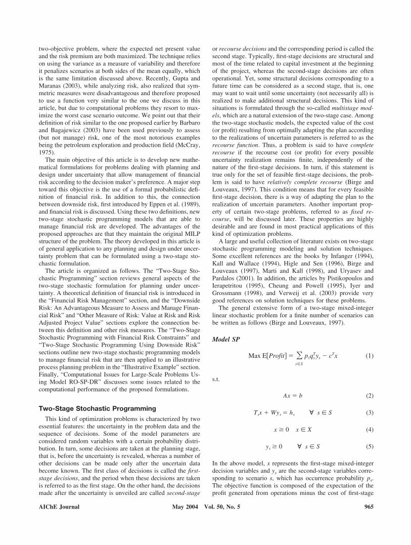
For conceptual purposes, the extension of this definition tothe case where the uncertainty is represented by a continuousprobabilistic distribution is now discussed. Intuitively, one maythink of this case as a limiting one, where the number ofscenarios becomes increasingly large, that is, Cardinality(S)3. Therefore, when profit has a continuous probability distri-bution, financial risk—defined as the probability of not meet-ing a target profit �—can be expressed as

Risk�x, ��

�

f�x, ��d� (11)

where f (x, �) is the profit probability distribution function(PDF), which is shown in Figure 2. The equivalent of the PDFin the discrete case is a histogram of frequencies similar to thatdepicted in Figure 1. A formal connection between the riskdefinition for the continuous case (Eq. 11) and the one for thediscrete scenario-based case (Eq. 9) is provided in Appendix A.

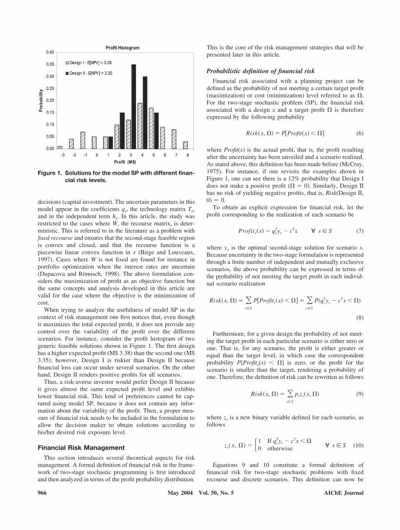
From the integral in Eq. 11, it follows that financial riskassociated to design x and a target profit � is given by the areaunder the curve f (x, �) from � � to � � �, as shown inFigure 2. Alternatively, in the discrete scenario case, financialrisk is given by the cumulative frequency obtained from theprofit histogram as depicted by Figure 3.

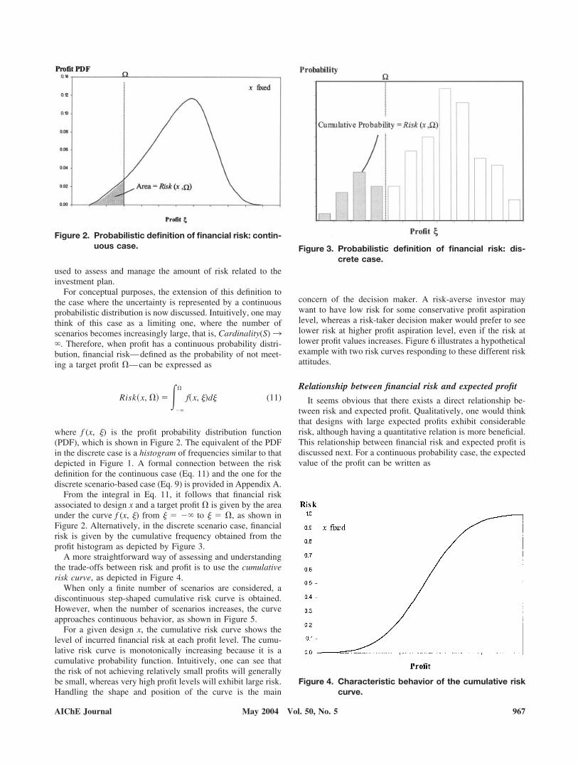
A more straightforward way of assessing and understandingthe trade-offs between risk and profit is to use the cumulativerisk curve, as depicted in Figure 4.

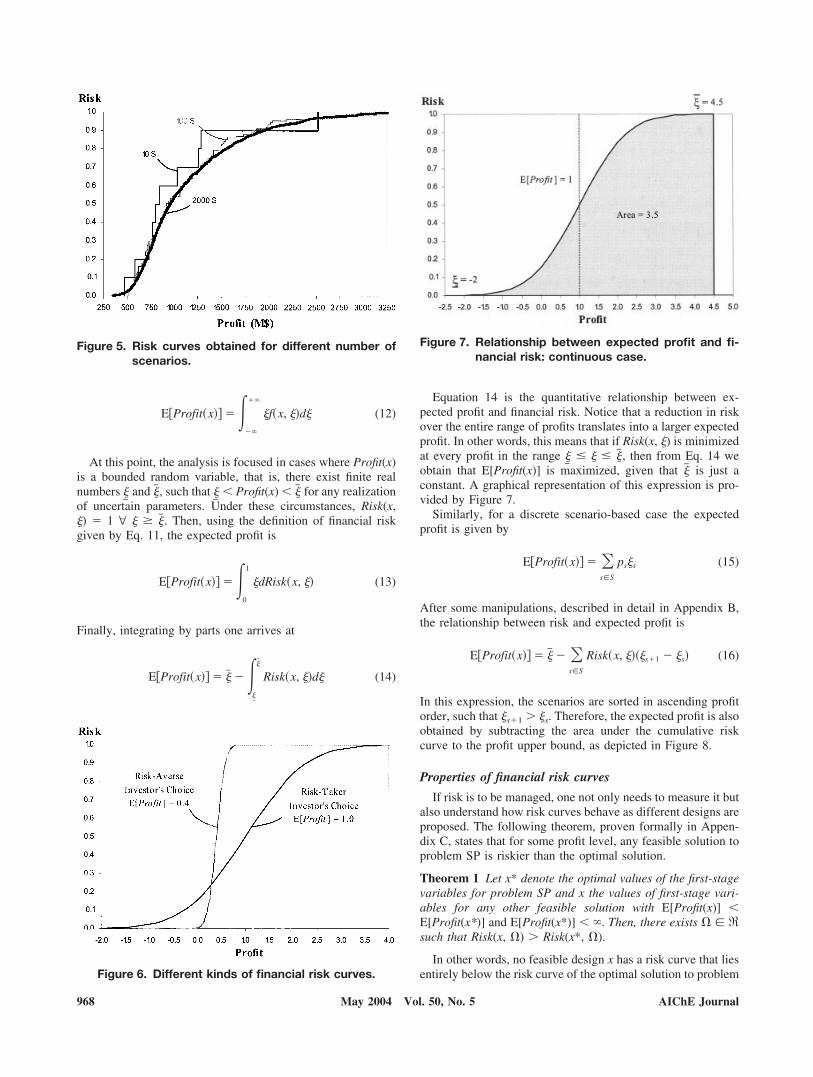
When only a finite number of scenarios are considered, adiscontinuous step-shaped cumulative risk curve is obtained.However, when the number of scenarios increases, the curveapproaches continuous behavior, as shown in Figure 5.

For a given design x, the cumulative risk curve shows thelevel of incurred financial risk at each profit level. The cumu-lative risk curve is monotonically increasing because it is acumulative probability function. Intuitively, one can see thatthe risk of not achieving relatively small profits will generallybe small, whereas very high profit levels will exhibit large risk.Handling the shape and position of the curve is the main

concern of the decision maker. A risk-averse investor maywant to have low risk for some conservative profit aspirationlevel, whereas a risk-taker decision maker would prefer to seelower risk at higher profit aspiration level, even if the risk atlower profit values increases. Figure 6 illustrates a hypotheticalexample with two risk curves responding to these different riskattitudes.

Relationship between financial risk and expected profit

It seems obvious that there exists a direct relationship be-tween risk and expected profit. Qualitatively, one would thinkthat designs with large expected profits exhibit considerablerisk, although having a quantitative relation is more beneficial.This relationship between financial risk and expected profit isdiscussed next. For a continuous probability case, the expectedvalue of the profit can be written as

Figure 2. Probabilistic definition of financial risk: contin-uous case. Figure 3. Probabilistic definition of financial risk: dis-

crete case.

Figure 4. Characteristic behavior of the cumulative riskcurve.


E�Profit�x��

�

�f�x, ��d� (12)

At this point, the analysis is focused in cases where Profit(x)is a bounded random variable, that is, there exist finite realnumbers

�� and �� , such that

�� Profit(x) � �� for any realization

of uncertain parameters. Under these circumstances, Risk(x,�) � 1 @ � � �� . Then, using the definition of financial riskgiven by Eq. 11, the expected profit is

E�Profit�x�� 0

1

�dRisk�x, �� (13)

Finally, integrating by parts one arrives at

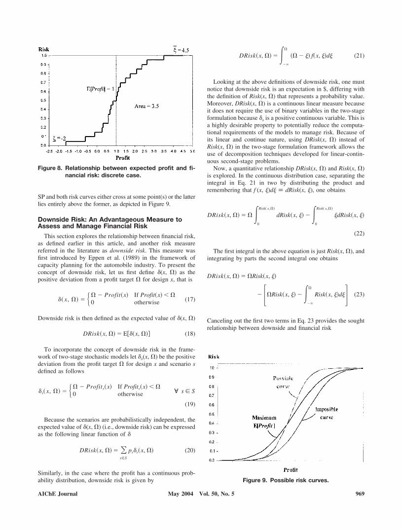
E�Profit�x��

��

Risk�x, ��d� (14)

Equation 14 is the quantitative relationship between ex-pected profit and financial risk. Notice that a reduction in riskover the entire range of profits translates into a larger expectedprofit. In other words, this means that if Risk(x, �) is minimizedat every profit in the range

�� , then from Eq. 14 we

obtain that E[Profit(x)] is maximized, given that �� is just aconstant. A graphical representation of this expression is pro-vided by Figure 7.

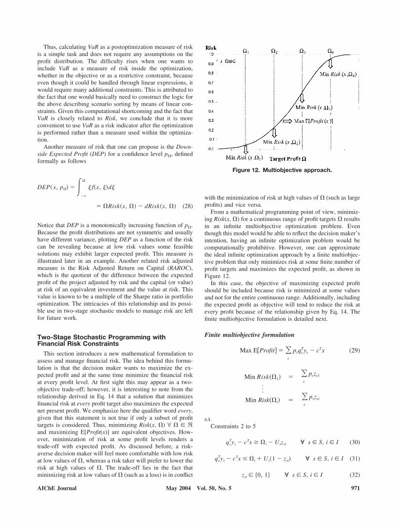
Similarly, for a discrete scenario-based case the expectedprofit is given by

E�Profit�x�� s�S

ps�s (15)

After some manipulations, described in detail in Appendix B,the relationship between risk and expected profit is


Risk�x, ��s�1 � �s� (16)

In this expression, the scenarios are sorted in ascending profitorder, such that �s�1 � �s. Therefore, the expected profit is alsoobtained by subtracting the area under the cumulative riskcurve to the profit upper bound, as depicted in Figure 8.

Properties of financial risk curves

If risk is to be managed, one not only needs to measure it butalso understand how risk curves behave as different designs areproposed. The following theorem, proven formally in Appen-dix C, states that for some profit level, any feasible solution toproblem SP is riskier than the optimal solution.

Theorem 1 Let x* denote the optimal values of the first-stagevariables for problem SP and x the values of first-stage vari-ables for any other feasible solution with E[Profit(x)] �E[Profit(x*)] and E[Profit(x*)] � . Then, there exists � � �such that Risk(x, �) � Risk(x*, �).

In other words, no feasible design x has a risk curve that liesentirely below the risk curve of the optimal solution to problem

Figure 5. Risk curves obtained for different number ofscenarios.

Figure 6. Different kinds of financial risk curves.

Figure 7. Relationship between expected profit and fi-nancial risk: continuous case.


SP and both risk curves either cross at some point(s) or the latterlies entirely above the former, as depicted in Figure 9.

Downside Risk: An Advantageous Measure toAssess and Manage Financial Risk

This section explores the relationship between financial risk,as defined earlier in this article, and another risk measurereferred in the literature as downside risk. This measure wasfirst introduced by Eppen et al. (1989) in the framework ofcapacity planning for the automobile industry. To present theconcept of downside risk, let us first define (x, �) as thepositive deviation from a profit target � for design x, that is

� x, �� Profit�x� If Profit�x� � �0 otherwise (17)

Downside risk is then defined as the expected value of (x, �)

DRisk�x, �� E��x, �� (18)

To incorporate the concept of downside risk in the frame-work of two-stage stochastic models let s(x, �) be the positivedeviation from the profit target � for design x and scenario sdefined as follows

s� x, �� Profits�x� If Profits�x� � �0 otherwise � s � S

(19)

Because the scenarios are probabilistically independent, theexpected value of (x, �) (i.e., downside risk) can be expressedas the following linear function of

DRisk�x, �� s�S

pss�x, �� (20)

Similarly, in the case where the profit has a continuous prob-ability distribution, downside risk is given by

DRisk�x, ��

�

�� f�x, ��d� (21)

Looking at the above definitions of downside risk, one mustnotice that downside risk is an expectation in $, differing withthe definition of Risk(x, �) that represents a probability value.Moreover, DRisk(x, �) is a continuous linear measure becauseit does not require the use of binary variables in the two-stageformulation because s is a positive continuous variable. This isa highly desirable property to potentially reduce the computa-tional requirements of the models to manage risk. Because ofits linear and continue nature, using DRisk(x, �) instead ofRisk(x, �) in the two-stage formulation framework allows theuse of decomposition techniques developed for linear-contin-uous second-stage problems.

Now, a quantitative relationship DRisk(x, �) and Risk(x, �)is explored. In the continuous distribution case, separating theintegral in Eq. 21 in two by distributing the product andremembering that f (x, �)d� dRisk(x, �), one obtains

DRisk�x, �� 0

Risk� x,��

dRisk�x, �� 0

Risk� x,��

�dRisk�x, ��

(22)

The first integral in the above equation is just Risk(x, �), andintegrating by parts the second integral one obtains

DRisk�x, �� Risk�x, ��

� ��Risk�x, ��

�

Risk�x, ��d�� (23)

Canceling out the first two terms in Eq. 23 provides the soughtrelationship between downside and financial risk

Figure 8. Relationship between expected profit and fi-nancial risk: discrete case.

Figure 9. Possible risk curves.


DRisk�x, ��

�

Risk�x, ��d� (24)

Therefore, downside risk is defined as the integral of finan-cial risk or area under the cumulative risk curve from profits� � to � � �, as shown in Figure 10.

In the previous section, Eq. 14 showed that the expectedprofit is related to the area under the cumulative risk curve fromprofits

�� to �� . Considering that downside risk is also defined as

the area under the risk curve, we obtain a straightforwardrelationship between expected profit and downside risk

E�Profit�x�� DRisk�x, �� (25)

At this point, an interesting observation concerning the re-lationship between downside and financial risk can be drawnkeeping in mind the decision maker’s intention to minimizerisk at every profit level. Because Risk(x, �) is an increasingfunction of the profit target, an intuitive way for reducing itover an entire continuous interval (

�� ) would be to

minimize the area under it, that is, to minimize the value of theintegral of Risk(x, �) from

�� to �� . This is the exact definition

of downside risk as given in Eq. 24. Then, one may presumethat minimizing DRisk(x, �) would be a convenient way ofaccomplishing the goal of minimizing financial risk. One mustnotice, however, that reducing the downside risk at a targetprofit � does not explicitly mean that financial risk is minimumat every single value of profit in the interval � � � �. Thisis because at a given value of � there might exist some riskcurves that having the same downside risk (that is, area) stillexhibit different financial risk at some profits below �. Ahypothetical example of this behavior is depicted in Figure 11for a profit target � � 0.5.

In view of the above discussion, one needs to analyze whatshould be the profit interval where minimizing downside riskhelps to find solutions that satisfy the risk preference of thedecision maker.

Other Measures of Risk: Value at Risk andDownside Expected Profit

Financial risk measured using the Risk function provides theprobability of achieving any given aspiration level. In the riskmanagement literature it is also usual to report the expectedvalue of profit connected to such probability or confidencelevel. A widely used measure of this kind is referred as Valueat Risk or VaR (Jorion, 2000), which was introduced by J. P.Morgan (Guldimann, 2000) and is defined as the expected lossfor a certain confidence level, usually set at 5% (Linsmeier andPearson, 2000). A more general definition of VaR is given bythe difference between the mean value of the profit and theprofit value corresponding to the p-quantile. For instance, aportfolio that has a normal profit distribution with zero meanand variance , VaR is given by zp, where zp is the number ofstandard deviations corresponding to the p-quantile of the profitdistribution. Most of the uses of VaR are concentrated onapplications where the profit probability distribution is as-sumed to follow a known distribution (usually the normal) sothat it can be calculated analytically. The relationship betweenVaR and Risk is generalized as follows

VaR�x, p�� E�Profit�x�� Risk1�x, �� (26)

where p� is the confidence level related to profit �, that is,p� � Risk(x, �). Notice that VaR requires the computation ofthe inverse function of Risk. Moreover, because Risk is amonotonically increasing function of �, one can see from Eq.26 that VaR is a monotonically decreasing function of p�.

For two-stage stochastic problems with a finite number ofscenarios, VaR can be easily estimated by sorting the scenariosin ascending profit order and simply taking the profit value ofthe scenario for which the cumulative probability equals thespecified confidence level; that is

VaR�x, p�� E�Profit�x�� Profitsp�x�

sp � �s� �k�1

s

pk � p�� (27)

Figure 10. Interpretation of downside risk.

Figure 11. Downside and financial risk.


Thus, calculating VaR as a postoptimization measure of riskis a simple task and does not require any assumptions on theprofit distribution. The difficulty rises when one wants toinclude VaR as a measure of risk inside the optimization,whether in the objective or as a restrictive constraint, becauseeven though it could be handled through linear expressions, itwould require many additional constraints. This is attributed tothe fact that one would basically need to construct the logic forthe above describing scenario sorting by means of linear con-straints. Given this computational shortcoming and the fact thatVaR is closely related to Risk, we conclude that it is moreconvenient to use VaR as a risk indicator after the optimizationis performed rather than a measure used within the optimiza-tion.

Another measure of risk that one can propose is the Down-side Expected Profit (DEP) for a confidence level p�, definedformally as follows

DEP� x, p��

�

� f�x, ��d�

� �Risk�x, �� dRisk�x, �� (28)

Notice that DEP is a monotonically increasing function of p�.Because the profit distributions are not symmetric and usuallyhave different variance, plotting DEP as a function of the riskcan be revealing because at low risk values some feasiblesolutions may exhibit larger expected profit. This measure isillustrated later in an example. Another related risk adjustedmeasure is the Risk Adjusted Return on Capital (RAROC),which is the quotient of the difference between the expectedprofit of the project adjusted by risk and the capital (or value)at risk of an equivalent investment and the value at risk. Thisvalue is known to be a multiple of the Sharpe ratio in portfoliooptimization. The intricacies of this relationship and its possi-ble use in two-stage stochastic models to manage risk are leftfor future work.

Two-Stage Stochastic Programming withFinancial Risk Constraints

This section introduces a new mathematical formulation toassess and manage financial risk. The idea behind this formu-lation is that the decision maker wants to maximize the ex-pected profit and at the same time minimize the financial riskat every profit level. At first sight this may appear as a two-objective trade-off; however, it is interesting to note from therelationship derived in Eq. 14 that a solution that minimizesfinancial risk at every profit target also maximizes the expectednet present profit. We emphasize here the qualifier word every,given that this statement is not true if only a subset of profittargets is considered. Thus, minimizing Risk(x, �) @ � � �and maximizing E[Profit(x)] are equivalent objectives. How-ever, minimization of risk at some profit levels renders atrade-off with expected profit. As discussed before, a risk-averse decision maker will feel more comfortable with low riskat low values of �, whereas a risk taker will prefer to lower therisk at high values of �. The trade-off lies in the fact thatminimizing risk at low values of � (such as a loss) is in conflict

with the minimization of risk at high values of � (such as largeprofits) and vice versa.

From a mathematical programming point of view, minimiz-ing Risk(x, �) for a continuous range of profit targets � resultsin an infinite multiobjective optimization problem. Eventhough this model would be able to reflect the decision maker’sintention, having an infinite optimization problem would becomputationally prohibitive. However, one can approximatethe ideal infinite optimization approach by a finite multiobjec-tive problem that only minimizes risk at some finite number ofprofit targets and maximizes the expected profit, as shown inFigure 12.

In this case, the objective of maximizing expected profitshould be included because risk is minimized at some valuesand not for the entire continuous range. Additionally, includingthe expected profit as objective will tend to reduce the risk atevery profit because of the relationship given by Eq. 14. Thefinite multiobjective formulation is detailed next.

Finite multiobjective formulation

Max E�Profit� � �s

psqsTys � cTx (29)

Min Risk��1� � �s

pszs1

···Min Risk��i� � �

s

pszsi

s.t.Constraints 2 to 5

qsTys � cTx � �i � Uszsi � s � S, i � I (30)

qsTys � cTx � �i � Us�1 � zsi� � s � S, i � I (31)

zsi � �0, 1� � s � S, i � I (32)

Figure 12. Multiobjective approach.


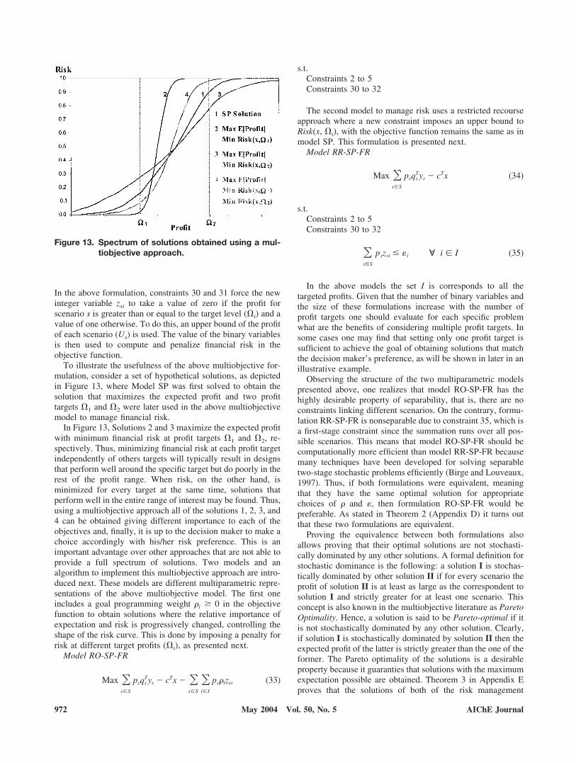
In the above formulation, constraints 30 and 31 force the newinteger variable zsi to take a value of zero if the profit forscenario s is greater than or equal to the target level (�i) and avalue of one otherwise. To do this, an upper bound of the profitof each scenario (Us) is used. The value of the binary variablesis then used to compute and penalize financial risk in theobjective function.

To illustrate the usefulness of the above multiobjective for-mulation, consider a set of hypothetical solutions, as depictedin Figure 13, where Model SP was first solved to obtain thesolution that maximizes the expected profit and two profittargets �1 and �2 were later used in the above multiobjectivemodel to manage financial risk.

In Figure 13, Solutions 2 and 3 maximize the expected profitwith minimum financial risk at profit targets �1 and �2, re-spectively. Thus, minimizing financial risk at each profit targetindependently of others targets will typically result in designsthat perform well around the specific target but do poorly in therest of the profit range. When risk, on the other hand, isminimized for every target at the same time, solutions thatperform well in the entire range of interest may be found. Thus,using a multiobjective approach all of the solutions 1, 2, 3, and4 can be obtained giving different importance to each of theobjectives and, finally, it is up to the decision maker to make achoice accordingly with his/her risk preference. This is animportant advantage over other approaches that are not able toprovide a full spectrum of solutions. Two models and analgorithm to implement this multiobjective approach are intro-duced next. These models are different multiparametric repre-sentations of the above multiobjective model. The first oneincludes a goal programming weight �i � 0 in the objectivefunction to obtain solutions where the relative importance ofexpectation and risk is progressively changed, controlling theshape of the risk curve. This is done by imposing a penalty forrisk at different target profits (�i), as presented next.

Model RO-SP-FR

Max �s�S

psqsTys � cTx � �

s�S

�i�I

ps�izsi (33)

s.t.Constraints 2 to 5Constraints 30 to 32

The second model to manage risk uses a restricted recourseapproach where a new constraint imposes an upper bound toRisk(x, �i), with the objective function remains the same as inmodel SP. This formulation is presented next.

Model RR-SP-FR

Max �s�S

psqsTys � cTx (34)


�s�S

pszsi � �i � i � I (35)

In the above models the set I is corresponds to all thetargeted profits. Given that the number of binary variables andthe size of these formulations increase with the number ofprofit targets one should evaluate for each specific problemwhat are the benefits of considering multiple profit targets. Insome cases one may find that setting only one profit target issufficient to achieve the goal of obtaining solutions that matchthe decision maker’s preference, as will be shown in later in anillustrative example.

Observing the structure of the two multiparametric modelspresented above, one realizes that model RO-SP-FR has thehighly desirable property of separability, that is, there are noconstraints linking different scenarios. On the contrary, formu-lation RR-SP-FR is nonseparable due to constraint 35, which isa first-stage constraint since the summation runs over all pos-sible scenarios. This means that model RO-SP-FR should becomputationally more efficient than model RR-SP-FR becausemany techniques have been developed for solving separabletwo-stage stochastic problems efficiently (Birge and Louveaux,1997). Thus, if both formulations were equivalent, meaningthat they have the same optimal solution for appropriatechoices of � and �, then formulation RO-SP-FR would bepreferable. As stated in Theorem 2 (Appendix D) it turns outthat these two formulations are equivalent.

Proving the equivalence between both formulations alsoallows proving that their optimal solutions are not stochasti-cally dominated by any other solutions. A formal definition forstochastic dominance is the following: a solution I is stochas-tically dominated by other solution II if for every scenario theprofit of solution II is at least as large as the correspondent tosolution I and strictly greater for at least one scenario. Thisconcept is also known in the multiobjective literature as ParetoOptimality. Hence, a solution is said to be Pareto-optimal if itis not stochastically dominated by any other solution. Clearly,if solution I is stochastically dominated by solution II then theexpected profit of the latter is strictly greater than the one of theformer. The Pareto optimality of the solutions is a desirableproperty because it guaranties that solutions with the maximumexpectation possible are obtained. Theorem 3 in Appendix Eproves that the solutions of both of the risk management

Figure 13. Spectrum of solutions obtained using a mul-tiobjective approach.


models presented above are always Pareto-optimal. Taking acloser look at models RO-SP-FR and RR-SP-FR, one realizesthat constraints 30 and 31 break the original fixed-recourseproperty of the problem because in these constraints the coef-ficients of the second-stage variables ys are stochastic. Giventhat having a fixed recourse matrix ensures the feasible regionof the second-stage problem is convex and closed (Birge andLouveaux, 1997), breaking this property seems at first sight tobe a considerable disadvantage of the proposed formulations.However, Theorem 4 in Appendix F proves that the feasibleregion of the model RO-SP-FR is the same as the feasibleregion of model SP and therefore it is still convex and closed.This is also true for model RR-SP-FR, given that the values of�i make this model equivalent to model RO-SP-FR.

Next, an algorithm for the implementation of the multiob-jective approach to financial risk management is presented. Inview of the advantages mentioned in the previous discussion,model RO-SP-FR is used in this procedure.

Risk Management Procedure Using the MultiobjectiveModel RO-SP-FR

(1) Solve the SP problem to obtain a solution that maxi-mizes the expected profit.

(2) Construct the corresponding risk curve. If the decisionmaker is satisfied with the current level of risk, then stop;otherwise, go to Step 3.

(3) Let the decision maker choose an arbitrary set of profittargets �i for which financial risk is to be reduced, if possible.Additionally, for every target define a sequence of ki weights�i

ki � {�i1, . . . , �i

ki} to manage the trade-off between expectedprofit and risk.

(4) Generate a set of n � �i ki instances of problem RO-SP-FR corresponding to all combinations of weights � for thedifferent profit targets. Solve all instances and construct theresulting risk curves associated with the optimal solution ofeach instance.

(5) Let the decision maker evaluate the results. If the deci-sion maker is satisfied with the risk curve of one or moresolutions, then stop; otherwise, go to Step 3.

In summary, the formulations presented in this section ad-dress the problem of controlling the financial risk curve of thesolutions to the two-stage stochastic problem such that thedecision maker can satisfy his/her risk preference. Computa-tionally, however, the inclusion of new integer variables couldin some cases represent a major limitation of these formula-tions. Adding integer second-stage variables eliminates thepossibility of using efficient decomposition techniques devel-oped for linear problems with continuous variables. Ap-proaches to solve stochastic programs with mixed-integer first-and second-stage variables were introduced by Caroe andSchultz (1997) and by Ahmed et al. (2000). However, thecomputational expense to solve large-scale problems usingthese methods is still significant. In additions, using General-ized Bender’s Decomposition to solve these models can guar-antee optimality only when the integer variables zsi are treatedas first-stage decisions because nonconvex second-stage sub-problems would arise otherwise. This limits the efficiency ofthe method for problems with large number of scenarios andfirst-stage decision variables that include integers. Thus, moreresearch effort should be directed to efficiently solve thesemixed-integer stochastic formulations. Nonetheless, for someapplications the computational limitations can be overcome

using presampling methods, such as the stochastic averageapproximation (Verweij et al., 2001), which yield modest sizeMILP instances. To ameliorate some of these problems analternative measure of risk is discussed next.

Two-Stage Stochastic Programming UsingDownside Risk

In this section we suggest that DRisk(x, �) be the measureused to control financial risk at different profit targets. Inaddition, Eq. 14 indicates that E[Profit(x)] may also be taken asa measure of financial risk at higher profit levels. Including theexpected profit in the objective would also help the modelchoose the solution with higher expectation in cases where twoor more solutions exhibit the same downside risk at a target �.The proposed model is as follows.

Model RO-SP-DR

Max ��s�S


s�S

pss (36)


s � � � cTx � qsTys � s � S (37)

s � 0 � s � S (38)

In this case also a procedure that generates a full spectrum ofsolutions is presented. This is accomplished by varying theprofit target � from small values around � � mins

{Profits( x*SP)} up to higher values around � � maxs

{Profits( x*SP)}. In this way, solutions obtained for lower val-ues of � will generally respond to a risk-averse investor andsolutions obtained with higher � will be more appealing torisk-taker investors.

Parametric algorithm for financial risk managementusing downside risk

(1) Solve the SP problem to obtain a solution that maxi-mizes the expected profit.

(2) Construct the corresponding risk curve. If the decisionmaker is satisfied with the current level of risk, then stop;otherwise, let k � 1 and go to Step 3.

(3) Define �0 � mins{Profits�x*SP)} and � 0.001 (oran equivalent small number).

(4) Choose a profit target �k � �k1. Let lk � 1.(5) Generate and solve problem RO-SP-DR using �k. Add

the new solution to the cumulative risk curve chart.(6) Let the decision maker evaluate the results. If the deci-

sion maker is satisfied with the risk curve of one or moresolutions, then stop; otherwise, let k � k � 1 and go to Step 4.

Quite clearly, different values of can possibly lead todifferent solution, even for the same profit target. The same istrue for different values of �i

ki in the case of the the RO-SP-FRmodel. Models with smaller value of will likely providesmaller ENPV. This is clearly another tool that the decision


maker has to obtain more risk curves to choose from, as weshall see below.

Illustrative Example

This section illustrates the usefulness of the proposed riskmanagement models using a capacity-planning problem. Con-sider the two-stage stochastic model presented by Liu andSahinidis (1996), which is an extension of the deterministicmixed-integer linear programming formulation introduced bySahinidis et al. (1989).

Model PP

Max ENPV � �s�1

NS �t�1

NT

psLt��l�1

NM �j�1

NC

��jltsSjlts � �jltsPjlts�

� �i�1

NP

itsWits� � �i�1

NP �t�1

NT

��itEit � �itYit� (39)

s.t.

YitEitL � Eit

L � YitEitU i � 1, . . . , NP t � 1, . . . , NT

(40)

Qit � Qi�t1� � Eit i � 1, . . . , NP t � 1, . . . , NT

(41)

�t�1

NT

Yit � NEXPi i � 1, . . . , NP (42)

�i�1

NP

��itEit � �itYit� � CIt t � 1, . . . , NT (43)

Wits�Qit

i � 1, . . . , NP t � 1, . . . , NT s � 1, . . . , NS (44)

�l�1

NM

Pjlts � �i�1

NP

�ijWits � �l�1

NM

Sjlts � �i�1

NP

ijWits

j � 1, . . . , NC t � 1, . . . , NT s � 1, . . . , NS (45)

ajltsL � Pjlts � ajlts

U j � 1, . . . , NC l � 1, . . . , NM

t � 1, . . . , NT s � 1, . . . , NS (46)

djltsL � Sjlts � djlts

U j � 1, . . . , NC l � 1, . . . , NM

t � 1, . . . , NT s � 1, . . . , NS (47)

Yit � �0, 1� i � 1, . . . , NP t � 1, . . . , NT (48)

Eit, Qit, Wits, Pjlts, Sjlts � 0 � i, j, l, t, s (49)

In this model, the objective function 39 maximizes theexpected net present value (ENPV) over the two stages of thecapacity expansion project, defined as the difference betweensales revenues and the investment, operating and raw materialcosts. The investment cost in terms of the design variables isrepresented by a variable term that is proportional to thecapacity expansion E and a fixed-charge term that taken intoaccount using binary decision variables Y. The second stage orrecourse cost is described as the expectation of the sales rev-enues and the expectation of the second-stage operating costsover finitely many, mutually exclusive scenarios s for eachtime period. Constraint 40 enforces lower and upper bounds inthe capacity expansion by means of the binary variables Y.Constraint 41 defines the total capacity available for process iduring time period t. Limits on the number of expansions ofprocesses and the capital budget are imposed by inequalities 42and 43, respectively. Constraint 44 ensures that the operatinglevel of a process does not exceed the installed capacity. Inturn, Eq. 45 expresses the material balances for each process,whereas constraints 46 and 47 enforce lower and upper boundsfor raw materials availability and products sales on each mar-ket. Observe that constraints 40 through 43 are expressed onlyin terms of first-stage variables; hence they are referred asfirst-stage constraints. On the other hand, constraints 44through 47 are indexed over all possible scenarios and are thencalled second-stage constraints. In the above formulation thedifferent scenarios between different time periods have beentreated independently because there are no second-stage con-straints linking time periods. Thus, a total of NS independentscenarios per time period are considered. Next, two models tomanage financial risk are presented, the first one using Risk(x,�) and the second one DRisk(x, �) as measures of risk.

Model RO-PP-FR

Max �s�1

NS �t�1

NT

psLs��l�1

NM �j�1

NC

��jltsSjlts � �jltsPjlts� � �i�1

NP

itsWits��

i�1

NP �t�1

NT

��itEit � �itYit� � �s�1

NS �n�1

NR

�npszsn (50)


�t�1

NT

Lt� �l�1

NM �j�1

NC


NP

itsWits��

i�1

NP �t�1

NT

��itEit � �itYit�

� �n � Us�1 � zsn�n � 1, . . . , NRs � 1, . . . , NS (51)


�t�1

NT

Lt� �l�1

NM �j�1

NC


NP

itsWits��

i�1

NP �t�1

NT

��itEit � �itYit� � �n � Uszsn

n � 1, . . . , NRs � 1, . . . , NS

(52)

zsn � �0, 1�n � 1, . . . , NRs � 1, . . . , NS (53)

Model RO-PP-DR

Max ��s�1

NS �t�1

NT

psLt��l�1

NM �j�1

NC

��jltsSjlts � �jltsPjlts�

� �i�1

NP

itsWits� � �i�1

NP �t�1

NT

��itEit � �itYit�� s�1

NS

pss (54)


s � � � �i�1

NP �t�1

NT

��itEit � �itYit� � �t�1

NT

Lt� �l�1

NM �j�1

NC

��jltsSjlts

� �jltsPjlts� � �i�1

NP

itsWits� s � 1, . . . , NS (55)

s � 0 s � 1, . . . , NS (56)

Example

This example consists of an investment project involvingfive chemical processes and eight chemicals arranged in aprocess network, as shown in Figure 14. The project is stagedin three periods of length one, two and a half, and three and ahalf years, respectively. The maximum number of expansionsallowed for each process is two and the capital limits at eachperiod are 100, 150, and 200 M$, respectively. The upperbound on capacity expansion is 100 kton/yr for all processes inall periods and none of the processes had initial capacityinstalled. Tables 1 and 2 show the fixed and variable invest-ment costs for each process, respectively, and Table 3 gives theoperational costs. Mass balance coefficients for products andraw materials are given in Tables 4 and 5. All these parametersare considered deterministic (i.e., nonstochastic). On the otherhand, market prices, availabilities, and demands were consid-ered as uncertain parameters characterized by a normal prob-ability distribution, with mean value and standard deviation asgiven in Tables 6 to 9. The uncertainty realizations for thisproblem were simulated through 400 independent scenariosgenerated by random sampling from the probability distribu-tions of the problem parameters.

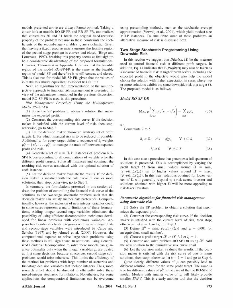
To manage financial risk for the above-described problem,model PP was solved first, obtaining the solution that maxi-mizes the expected net present value, without taking financialrisk into account. This solution, the risk curve for which isshown in Figure 15, is detailed in Table 10 and graphicallyrepresented in Figure 16.

After solving model PP the idea is then to explore the riskbehavior of other solutions by using models RO-PP-FR andRO-PP-DR. In this way, the decision maker is provided a seriesof solutions reflecting different levels of risk exposure to makea selection according to his/her criteria. First, the results usingmodel RO-PP-FR are presented.

Results using model RO-PP-FR

To explore different alternatives using this model, financialrisk at several NPV targets from 600 to 1500 M$ was mini-mized (with weight � � 10,000) considering one target at atime. The results for each target are shown in Table 11, where

Figure 14. Process network for the example.

Table 1. Fixed Investment Cost Coefficients

Process

�it (k$)

t1 t2 t3

i1 20,000 19,000 18,000i2 21,000 19,000 17,000i3 40,000 39,500 39,000i4 44,000 42,500 40,000i5 48,000 46,000 44,000

Table 2. Variable Investment Cost Coefficients

Process

�it (k$ � yr/kton)

t1 t2 t3

i1 800 795 790i2 780 770 760i3 1400 1360 1320i4 1360 1340 1320i5 1300 1290 1280

Table 3. Operation Cost Coefficients

Process

it (k$ � yr/kton)

t1 t2 t3

i1 2000 2200 2400i2 2100 2000 1900i3 1500 1400 1300i4 1300 1300 1300i5 1400 1200 1100


the solution for model PP is also included for comparisonpurposes. The risk curves corresponding to the different solu-tions are shown in Figure 17. A total of 200 scenarios was usedin all instances of problem RO-PP-FR.

Observe that for this example, solutions obtained by mini-mizing financial risk at targets below the maximum expectednet present value of M$ 1140 exhibit lower risk of realizing asmall NPV. On the other hand, when risk was minimized athigher NPV targets the solutions showed considerably higherrisk at small profits and only a small reduction in risk at higherNPV values with respect to the solution given by model PP.Thus, minimizing risk at large NPV targets brings about higherrisk at lower NPV values. This is in agreement with the theo-retical behavior described in previous sections. Then, one canconclude that for this example it does not seem worthwhile tochoose solutions that minimize risk at NPV targets higher thanM$ 1000.

To further analyze the results, notice from Table 12 that asthe NPV target (�) is incremented, the expected net presentvalue of the solutions approaches to the maximum value ob-tained with model PP. This is attributed to the relationshipbetween financial risk and expected profit established by Eq.14, which shows that as the profit target increases and financialrisk approaches unity, minimizing risk becomes equivalent tomaximizing the expected profit.

So far, a set of solutions showing different risk characteris-tics was obtained. This set should next be analyzed by thedecision maker and some solution(s) selected. In a situationwhere none of the solutions satisfies the decision maker’spreference, more solutions should be explored using differenttargets � and weights � as described in “Two-Stage StochasticProgramming with Financial Risk Constraints.” The procedureshould be repeated until the decision maker is satisfied orfinancial risk cannot be managed further. One can concludefrom Figure 17 that most of the risk behavior for this examplehas been already captured by the shown solutions.

One final observation can be made regarding the risk behav-ior of the decision makers: it is usually assumed that decisionmakers are risk-averse, that is, they want to lower their expo-sure to losses. However, this characteristic may be problem-dependent: for instance, in this example all solutions guarantee

profit under every scenario. Moreover, solutions reducing riskto almost zero at a target of � � 600 M$ also exhibit aprobability greater than 50% of not making a profit larger thanM$ 1000. On the other hand, the solution obtained withoutpenalizing risk (using model SP), has only around 10% risk atthis profit target, but a respectable chance of making muchhigher profits. Therefore, even a risk-averse decision makermay become a risk taker under these circumstances. Thisreasoning shows the importance of obtaining a full spectrum ofsolutions such as the one generated using the proposed models,and the need to present them to the decision maker so he/shecan make the final choice.

Results using model RO-PP-DR

This section presents the results obtained with model RO-PP-DR. The strategy in this case was to handle the risk curvesby minimizing the downside risk at several NPV targets from600 to 1500 M$ with weight � 0.001 for the expected NPV.The results for each target are shown in Table 12 and thecorresponding risk curves plotted in Figure 18. The total num-ber of scenarios in all instances was 400.

Looking at Figure 18 one may notice that some risk curvesare similar to those presented in the previous section; however,in this case all the curves lay below the curve with maximumENPV (obtained with model PP) for small NPV values. Recallthat when model RO-PP-FR was used to minimize financialrisk at high NPV targets it produced solutions with high risk atsmall NPV values. These solutions were not found using modelRO-PP-DR because they lead to such a small reduction in riskfor large NPV values that the area under the risk curve (that is,the downside risk) turns out to be almost always higher thanthat of other solutions. Not finding these curves is not disad-vantageous for this problem because they show no improve-ment from a risk perspective.

Two different kinds of probability distributions can be wellidentified in Figure 18: solutions for � � 600–900 M$ behaveas normally distributed random variables, whereas the rest ofthe solutions respond to a different kind of distribution. Threesolutions have been selected to more clearly depict this obser-vation in Figures 19 and 20. A schematic representation of thesolutions for � � 900 and 1100 is given in Figures 21 and 22,respectively.

Table 4. Raw Material Stoichiometric Coefficients

Process

ij

j1 j2 j3 j4 j5 j6 j7 j8

i1 1i2 1i3 1i4 1i5 1

Table 5. Product Stoichiometric Coefficients

Process

�ij

j1 j2 j3 j4 j5 j6 j7 j8

i1 1i2 1 1i3 1i4 1i5 1 1

Table 6. Expected Purchase Prices and Availabilities

Market l1

Chemical

Price (k$/kton)Availability

(kton/yr)

t1 t2 t3 t1 t2 t3

j1 4000 4300 4600 50 60 70j2 5000 5500 6000 60 80 100j3 6000 6100 6200 40 42 44

Table 7. Expected Sale Prices and Demands

Market l1

Chemical

Price (k$/kton) Demand (kton/yr)

t1 t2 t3 t1 t2 t3

j5 6000 6200 6400 75 90 105j6 14000 14500 15000 30 60 90j7 8000 8100 8200 80 85 90j8 24000 24200 24400 120 130 140


A final observation based on Figure 17 is that as the NPVtargeted is increased, the resulting risk curves approach to thecurve with maximum ENPV. This is predicted by Eq. 25 of thefirst part, which establishes the relationship between downsiderisk and expected profit and shows that minimizing downsiderisk at high profit targets is equivalent to maximizing theexpected profit.

Finally, one can conclude that using model RO-PP-DR al-lows managing financial risk because a set of solutions show-ing different risk curves was obtained. In the next section, thismodel is used to examine the effect of inventory on the riskcurves.

Downside expected profit

The DEP is shown in Figure 23 for the optimal solution ofmodel PP and a solution obtained using model RO-PP-FR with� � 900, which has an expected value of M$ 908. Consider forinstance any level of risk, say 50%. The risk downside ex-pected profit DEP(x, 50%) is the expected profit with a levelrisk of 50%. Notice that in this way, the actual expected profit(ENPV) is given by DEP(x, 100%). For this reason, the PPsolution (which has the maximum expected net present value)has the highest value of DEP(x, 100%). However, at otherlevels of confidence (from 0% up to about 67%) the solutionfor � � 900 has a higher expected profit. This kind of plots,therefore, provides the decision maker additional insight aboutthe risk exposure of each solution.

Computational Issues for Large-Scale ProblemsUsing Model RO-SP-DR

Two methods are presented in this section aiming at obtain-ing improved computational performance when solving large-scale risk management problems with a large number of sce-narios. First the Sampling Average Approximation method isintroduced and later a solution algorithm that exploits thedecomposable structure of model RO-SP-DR is described.

Sampling average approximation (SAA) method

In large-scale optimization of stochastic problems, samplingmethods coupled with mathematical decomposition have beenwidely applied to many applications and incorporated in sev-

eral algorithms [see Birge and Louveaux (1997), Higle and Sen(1996), and Infanger (1994) for reviews of these techniques].Recently, Verweij et al. (2001) reported excellent computa-tional results for different classes of large-scale stochasticrouting problems using the sampling average approximationmethod (SAA). Additionally, the stochastic decompositionmethod (L-shaped) using Monte Carlo sampling (Higle andSen, 1996) or importance sampling (Infanger, 1991) may showimproved computational efficiency in some cases. In this arti-cle, the SAA method using Monte Carlo sampling was imple-mented and tested.

In the SAA technique, the expected second-stage profit (re-course function) in the objective function is approximated byan average estimate of NS independent random samples of theuncertain parameters, and the resulting problem is called the“approximation problem.” Here, each sample corresponds to apossible scenario and so NS is the total number of scenariosconsidered. Then, the resulting approximation problem issolved repeatedly for M different independent samples (each ofsize NS) as a deterministic optimization problem. In this way,the average of the objective function of the approximationproblems provides an estimate of the stochastic problem ob-jective. Notice that this procedure may generate up to Mdifferent candidate solutions. To determine which of these M(or possibly less) candidates is optimal in the original problem,the values of the first-stage variables corresponding to each

Figure 15. Solution that maximizes the expected netpresent value.

Table 8. Standard Deviation of PurchasePrices and Availabilities

Market l1

Chemical

Price (k$/kton) Availability (kton/yr)

t1 t2 t3 t1 t2 t3

j1 1000 1075 1150 12.5 15 17.5j2 1250 1375 1500 15 20 25j3 300 305 310 2 2.1 2.2

Table 9. Standard Deviation of Sale Prices and Demands

Market l1

Chemical

Price (k$/kton) Demand (kton/yr)

t1 t2 t3 t1 t2 t3

j5 1500 1550 1600 18.75 22.5 26.25j6 3500 3625 3750 7.5 15 22.5j7 400 405 410 4 4.25 4.5j8 1200 1210 1220 6 6.5 7

Table 10. Solution Using Model PP

Process Expanded at Period

i1 t1, t3

i2 t3

i3 t1

i4 t2

i5 t2

E[NPV] 1140 M$E[Sales] 5833 M$E[Purchases] 3131 M$E[Operation Cost] 1162 M$Investment 400 M$


candidate solution are fixed and the problem is solved againusing a larger number of scenarios NS� �� NS to distinguishthe candidates better. After solving these new problems, anestimate of the optimal solution of the original problem (x*) isobtained. Therefore, x* is given by the solution of the approx-imate problems that yields the highest objective value for theapproximation problem with NS� samples. This algorithm ispresented next.

SAA algorithm

Select NS, NS�, MFor m � 1 to M

For s � 1 to NSUse Monte Carlo sampling to generate an independentobservation of the uncertain parameters, �s,m � (qs, Ts,hs). Define ps � 1/NS.

Next sSolve problem RO-SP-DR with NS scenarios. Let the xm

be the optimal first-stage solution.Next mFor m � 1 to M

For s � 1 to NS�Use Monte Carlo sampling to generate an independentobservation of the uncertain parameters, �s,m � (qs, Ts,hs). Define ps � 1/NS�.

Next sSolve problem RO-SP-DR with NS� scenarios, fixing xm

as the optimal first-stage solution.Next mUse x* � argmax{Obj(xm) m � 1, 2, . . . , M} as theestimate of the optimal solution to the original problemwhere Obj(x*) is the estimate of the optimal objective value.End

Results

The performance of the above SAA algorithm was evaluatedfor the illustrative example considering the stochastic program-

Figure 16. Solution that maximizes the expected netpresent value.

Figure 17. Solutions obtained using model RO-PP-FR.

Table 11. Solutions Obtained Using Formulation RO-PP-FR

�1 PP 600 700 800 900 1000 1100 1200 1300 1400 1500�1 — 10000 10000 10000 10000 10000 10000 10000 10000 10000 10000

Process Period(s) in Which Capacity Expansion Is Performedi1 t1, t3 t1 t1 t1, t3 t1, t2 t1, t2 t1, t2 t1, t2 t1, t2 t1, t2 t1

i2 — t3 t3 t1, t2 t1, t2 t1, t2 t1, t2 t1, t2 t1, t2 t1, t3 t2

i3 t1 t1 t1 t1 t2 t2 T2 t2 t2 t2 t2

i4 t2 t2 t2 t2 t3 t3 T3 t3 t3 t3 t3

i5 t2 t2 t2 t2 t3 t3 T3 t3 t3 t3 t3

E[NPV] M$ 1140 876 906 1000 1064 1081 1081 1071 1066 1069 1075E[Sales] M$ 5833 3693 3971 4702 6191 6220 6169 6201 6173 6314 6226E[Purchases] M$ 3131 1947 2104 2509 3387 3387 3349 3381 3363 33495 3403E[Operation Cost] M$ 1162 624 689 868 1343 1358 1345 1352 1348 1370 1362Investment M$ 400 247 272 325 397 394 394 397 396 439 385


ming and the downside risk models. Eight different samplesizes (i.e., total number of scenarios) from 50 to 400 wereconsidered and the problems for each sample were repeatedlysolved 20 times (M � 20). Finally, the optimal first-stagesolution (referred to here as Sol1) was determined by solvingthe models for each of the candidate solutions with NS� �2000. The rest of the candidate solutions are labeled Sol2, Sol3,and so forth, according to their frequency. For this problem, thestructure of the candidate solutions is given by the binaryvariables Yit, representing the decision of constructing or ex-panding process i at period t. For each model, the sampleaverage and standard deviation of the ENPV were computed asfollows

ENPV Average � �m�1

M

ENPVm (57)

ENPV Std Dev � �¥m�1M �ENPVm � ENPV Average�2

M � 1

(58)

Similar equations were used to compute the average andstandard deviation for DRisk, as shown next

DRisk Average � �m�1

M

DRiskm (59)

DRisk Std Dev � �¥m�1M �DRiskm � DRisk Average�2

M � 1

(60)

The results for the different models are presented in Tables 13through 15.

By analyzing the results presented in the above tables onecan see that in this example the SAA method performs verywell in terms of differentiating the optimal first-stage solution(Sol1) from the rest of the candidates. Notice that in all casesthe optimal solution appears with a much higher frequency thanthat of the rest of the candidates and that for samples with NS �150 it is almost the only solution found. Additionally, in mostcases only two solutions are selected as candidates, which is a

Figure 18. Solutions obtained using model RO-PP-DR.Figure 19. Selected solutions obtained using model RO-

PP-DR.

Table 12. Solutions Obtained Using Formulation RO-PP-DR (Downside Risk Approach)

Profit Target

�

PP 500 600 700 800 900 1000 1100 1200 1300 1400 1500

Process Period(s) in Which Capacity Expansion Is Performed

i1

t1,t3 — t1 t1 t1 t1

t1,t3

t1,t3

t1,t3

t1,t3

t1,t3

t1,t3

i2 t3 — — t3 t3 t3 t3 t3 t3 t3 t3 t3

i3 t1 t1 t1 t1 t1 t1 t1 t1 t1 t1 t1 t1

i4 t2 t2 t2 t2 t2 t2 t2 t2 t2 t2 t2 t2

i5 t2 t2 t2 t2 t2 t2 t2 t2 t2 t2 t2 t2

E[NPV] 1140 855 875 897 908 9008 1032 1074 1099 1107 1122 1125E[Sales] 5833 3472 3698 3916 3977 3981 4936 5221 5407 5378 5591 5610E[Purchases] 3131 1843 1946 2072 2108 2110 2637 2795 287 2867 2999 3010E[Operation Cost] 1162 551 631 675 689 690 932 1005 1052 1039 1099 1104Investment 400 222 246 271 273 273 334 348 358 363 370 372


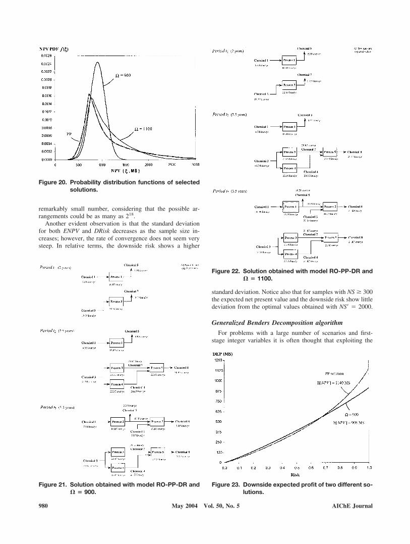
remarkably small number, considering that the possible ar-rangements could be as many as 218.

Another evident observation is that the standard deviationfor both ENPV and DRisk decreases as the sample size in-creases; however, the rate of convergence does not seem verysteep. In relative terms, the downside risk shows a higher

standard deviation. Notice also that for samples with NS � 300the expected net present value and the downside risk show littledeviation from the optimal values obtained with NS� � 2000.

Generalized Benders Decomposition algorithm

For problems with a large number of scenarios and first-stage integer variables it is often thought that exploiting the

Figure 20. Probability distribution functions of selectedsolutions.

Figure 21. Solution obtained with model RO-PP-DR and� � 900.

Figure 22. Solution obtained with model RO-PP-DR and� � 1100.

Figure 23. Downside expected profit of two different so-lutions.


decomposable structure of the problem could help reduce thecomputational effort to solve it. In this sense, GeneralizedBenders Decomposition (GBD) (Benders, 1962; Geoffrion,1972) has been found to be efficient to solve some MILPproblems arising in stochastic programming (Liu and Sahini-dis, 1996). Generally, the computational efficiency of thisalgorithm is highly dependent on the specific structure andcharacteristics of the problem. Hence, strategies that combinethe GBD algorithm with other approaches such as branch andcut (Verweij et al., 2001), addition of integer cuts (Iyer andGrossman, 1989), or heuristics (Ahmed and Sahinidis, 2000a),designed for the specific application, may greatly improvecomputational performance.

As a first step, the incorporation of GBD to solve large-scaleinstances of risk management model RO-SP-DR in the pro-posed SAA algorithm is suggested, and two different GBDalgorithms are explored. In the first one, the first-stage vari-ables are taken as complicating variables, rendering a Benders’Primal problem with only second-stage constraints and vari-ables, which is then solved simultaneously for all scenarios.This algorithm will be referred to in this article as “Benders.”In addition, the second GBD algorithm also considers thefirst-stage variables as complicating ones, although the result-ing Benders’ Primal problem is solved separately for eachscenario, taking advantage of the decomposable structure of theproblem. This algorithm is referred to here as “Benders-SD”and corresponds to a stochastic decomposition of the originalproblem. Before presenting the structure of the GBD algo-rithms, the optimization problems that are used inside thealgorithm are defined.

Optimality Primal P(k)

Max �s�S

psqsTys

k � �s�S

pssk (61)

s.t.

Wysk � hs � Tsx

k � s � S (62)

sk � qs

Tysk � � � cTxk � s � S (63)

ysk, s

k � 0 � s � S (64)

Feasibility Primal F(k)

Min �s�S

�eT�s� � eT�s � eT�s

� (65)

s.t.

Wysk � I�s

� � I�s � hs � Tsx

k � s � S (66)

sk � qs

Tysk � I�s � � � cTxk � s � S (67)

ysk, si

k , �s�, �s

, �s � 0 � s � S (68)

Master Problem M(k)

Max � (69)

s.t.

Axk � b (70)

Table 13. SAA Method Results for Model PP

NSNS� M ENPV Average ENPV Std Dev

Candidate Solutions Frequency

Sol1 Sol2 Sol3 Sol4

50 20 1177.1 78.3 13 4 2 1100 20 1144.4 56.7 18 2 — —150 20 1144.7 31.9 20 — — —200 20 1152.3 33.1 20 — — —250 20 1156.2 30.5 20 — — —300 20 1150.3 24.2 20 — — —350 20 1157.6 30.8 20 — — —400 20 1154.3 30.9 20 — — —

2000 — 1152.4 — — — — —

Table 14. SAA Method Results for Model RO-PP-DR (� � 900, � � 0.001)

NSNS� M ENPV Average ENPV Std Dev DRisk Average DRisk Std Dev

Candidate Solutions Frequency

Sol1 Sol2 Sol3 Sol4

50 20 972.7 78.5 53.1 12.7 8 6 4 2100 20 932.9 42.5 57.0 7.1 15 5 — —150 20 917.6 28.7 56.5 5.3 19 1 — —200 20 927.4 48.7 58.6 4.0 16 3 — 1250 20 931.0 36.6 57.6 6.2 16 4 — —300 20 919.6 27.8 57.6 5.1 18 2 — —350 20 924.5 33.2 56.6 5.3 18 2 — —400 20 915.3 22.5 58.6 4.1 18 2 — —

2000 — 914.2 — 58.1 — 1 — — —


� � cTxk � �s�S

��s1,k�hs � Tsx

k� � �s2,k�� cTxk��

k � Ko (71)

0 � �s�S

�s1,k�hs � Tsx

k� � s2,k�� cTxk�� k � Kf

(72)

xk � 0 xk � X (73)

The above problems are used in each iteration (k) of theBenders algorithm. The first problem, P(k) or Optimality Pri-mal is used to generate an optimality cut constraint that is alinear approximation of the recourse function. If subproblemP(k) turns out to be infeasible, then a feasibility primal problemF(k) is solved to generate a feasibility cut that reduces thefeasible region of the master problem, eliminating infeasibili-ties in the second-stage. Finally, the master problem M(k) isiteratively solved to update the first-stage decisions until opti-mality is achieved.

The optimization problems for the Benders-SD algorithm arepresented next. In this case, the optimality and feasibilityproblems are solved independently for each different scenario.

Optimality Primal P(k, s)

Max qsTys

k � sk (74)

s.t.

Wysk � hs � Tsx

k (75)

sk � qs

Tysk � � � cTxk (76)

ysk, s

k � 0 (77)

Feasibility Primal F(k, s)

Min eT�s� � eT�s � eT�s

(78)

s.t.

Wysk � I�s

� � I�s � hs � Tsx

k (79)

sk � qs

Tysk � I�s � � � cTxk (80)

ysk, si

k , �s�, �s

, �s � 0 (81)

Master Problem M(k)

Max � (82)

s.t.

Axk � b (83)

� � cTxk � �s

ps��s1,k�hs � Tsx

k� � �s2,k�� cTxk��

k � Ko (84)

0 � s1,k�hs � Tsx

k� � s2,k�� cTxk� s � Sk, k � Kf (85)

xk � 0 xk � X (86)

Having properly defined the correspondent optimizationproblems, the GBD algorithms are presented next.

Benders algorithm

Initialization Set k3 1 and choose x1 � {x Ax � b, x � 0}.Set UB 3 and LB 3 . Let the set of optimality andfeasibility cuts be Ko 3 {�} and Kf 3 {�}, respectively.

Step 1 Solve optimality primal P(k).If P(k) is feasible, then:

● Let �s1,k and �s

2,k be the optimal Lagrange multipliersassociated with constraints 62 and 63, respectively.

● Set Ko 3 Ko � {k}.● Let ys

k* and sk* be the optimal values of the variables in

P(k) and go to Step 2.Else,

● Solve the feasibility cut primal F(k).● Let s

1,k and s2,k be the optimal Lagrange multipliers

associated with constraints 66 and 67, respectively.● Set Kf 3 Kf � {k} and go to Step 3.Step 2 Let LB � max{LB, (¥s psqs

Tysk* cTxk) ¥s

pssk*}. If UB LB � tolerance, then terminate with xk being

an optimal solution to the problem.

Table 15. SAA Method Results for Model RO-PP-DR (� � 1100, � � 0.001)

NSNS� M ENPV Average ENPV Std Dev DRisk Average DRisk Std Dev

Candidate SolutionsFrequency

Sol1 Sol2 Sol3

50 20 1055.5 74.5 176.8 25.9 14 4 2100 20 1055.5 59.2 180.0 23.6 19 1 —150 20 1076.4 36.5 172.0 13.5 20 — —200 20 1073.7 47.2 175.0 17.8 20 — —250 20 1074.8 35.0 171.8 14.2 20 — —300 20 1088.2 23.3 167.8 11.6 20 — —350 20 1086.1 27.9 169.0 10.5 20 — —400 20 1081.0 28.4 172.0 9.3 20 — —

2000 — 1092.9 — 168.2 — 1 — —


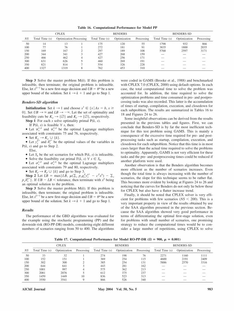
Step 3 Solve the master problem M(k). If this problem isinfeasible, then terminate; the original problem is infeasible.Else, let xk�1 be a new first-stage decision and UB � �* be a newupper bound of the solution. Set k3 k � 1 and go to Step 1.

Benders-SD algorithm

Initialization Set k 3 1 and choose x1 � {x Ax � b, x �0}. Set UB 3 and LB 3 . Let the set of optimality andfeasibility cuts be Ko 3 {�} and Kf 3 {�}, respectively.

Step 1 For each s solve optimality primal P(k, s).If P(k, s) is feasible @ s, then:

● Let �s1,k and �s

2,k be the optimal Lagrange multipliersassociated with constraints 75 and 76, respectively.

● Set Ko 3 Ko � {k}.● Let ys

k* and sk* be the optimal values of the variables in

P(k, s) and go to Step 2.Else,

● Let Sk be the set scenarios for which P(k, s) is infeasible.● Solve the feasibility cut primal F(k, s) @ s � Sk.● Let s

1,k and s2,k be the optimal Lagrange multipliers

associated with constraints 79 and 80, respectively.● Set Kf 3 Kf � {k} and go to Step 3.Step 2 Let LB � max{LB, (¥s psqs

Tysk* cTxk) ¥s

pssk*}. If UB LB � tolerance, then terminate with xk being

an optimal solution to the problem.Step 3 Solve the master problem M(k). If this problem is

infeasible, then terminate; the original problem is infeasible.Else, let xk�1 be a new first-stage decision and UB � �* be a newupper bound of the solution. Set k3 k � 1 and go to Step 1.

Results

The performance of the GBD algorithms was evaluated forthe example using the stochastic programming (PP) and thedownside risk (RO-PP-DR) models, considering eight differentnumbers of scenarios ranging from 50 to 400. The algorithms

were coded in GAMS (Brooke et al., 1988) and benchmarkedwith CPLEX 7.0 (CPLEX, 2000) using default options. In eachcase, the total computational time to solve the problem wasaccounted for. In addition, the time required to solve theoptimization problems and time consumed in pre- and postpro-cessing tasks was also recorded. This latter is the accumulationof times of startup, compilation, execution, and closedown foreach subproblem. The results are summarized in Tables 16 to18 and Figures 24 to 26.

Some insightful observations can be derived from the resultspresented in the previous tables and figures. First, we canconclude that Benders-SD is by far the most inefficient tech-nique for this test problem using GAMS. This is mainly aconsequence of the excessive time required for pre- and post-processing tasks such as startup, compilation, execution, andclosedown for each subproblem. Notice that this time is in mostcases larger than the actual time required to solve the problemsto optimality. Apparently, GAMS is not very efficient for thesetasks and the pre- and postprocessing times could be reduced ifanother platform were used.

Another observation is that the Benders algorithm becomesmore efficient as the number of scenarios increases. Eventhough the total time is always increasing with the number ofscenarios, the slope for this technique seems to be rather flat.This becomes more evident by looking at Figures 24 to 26 andnoticing that the curves for Benders do not only lie below thosefor CPLEX but also have a flatter increase trend.

Finally, it should be noted that CPLEX solver is very effi-cient for problems with few scenarios (NS � 200). This is avery important property in view of the results obtained by useof the SAA algorithm presented in the previous section. Be-cause the SAA algorithm showed very good performance interms of differentiating the optimal first-stage solution, evenfor problems with small number of scenarios, one promisingstrategy to reduce the computational times would be to con-sider a large number of repetitions, using CPLEX to solve

Table 16. Computational Performance for Model PP

NS

CPLEX BENDERS BENDERS-SD

Total Time (s) Optimization Processing Total Time (s) Optimization Processing Total Time (s) Optimization Processing

50 14 13 1 175 120 55 1798 932 866100 77 76 1 272 181 91 3835 1800 2035150 169 167 2 297 189 108 5768 2597 3171200 344 341 3 427 268 159 — — —250 466 462 4 427 256 171 — — —300 631 626 5 460 269 191 — — —350 821 814 7 554 326 228 — — —400 1327 1319 8 762 453 310 — — —

Table 17. Computational Performance for Model RO-PP-DR (� � 900, � � 0.001)

NS



50 33 32 1 274 198 76 2271 1160 1111100 152 151 1 369 254 115 4600 2191 2409150 302 300 2 385 254 131 5886 2570 3316200 644 641 3 443 281 162 — — —250 1001 997 4 575 362 213 — — —300 2081 2076 5 612 375 237 — — —350 1459 1449 10 836 523 313 — — —400 3550 3541 9 866 526 340 — — —


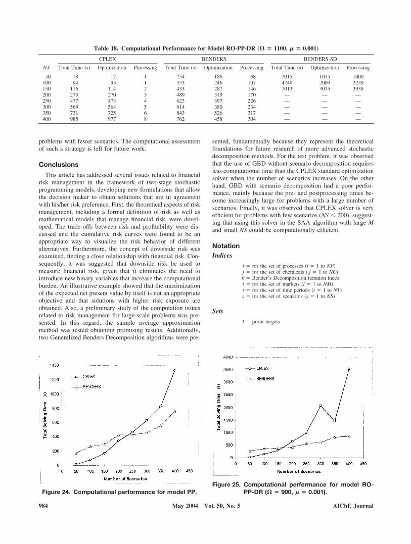
problems with fewer scenarios. The computational assessmentof such a strategy is left for future work.

Conclusions

This article has addressed several issues related to financialrisk management in the framework of two-stage stochasticprogramming models, developing new formulations that allowthe decision maker to obtain solutions that are in agreementwith his/her risk preference. First, the theoretical aspects of riskmanagement, including a formal definition of risk as well asmathematical models that manage financial risk, were devel-oped. The trade-offs between risk and profitability were dis-cussed and the cumulative risk curves were found to be anappropriate way to visualize the risk behavior of differentalternatives. Furthermore, the concept of downside risk wasexamined, finding a close relationship with financial risk. Con-sequently, it was suggested that downside risk be used tomeasure financial risk, given that it eliminates the need tointroduce new binary variables that increase the computationalburden. An illustrative example showed that the maximizationof the expected net present value by itself is not an appropriateobjective and that solutions with higher risk exposure areobtained. Also, a preliminary study of the computation issuesrelated to risk management for large-scale problems was pre-sented. In this regard, the sample average approximationmethod was tested obtaining promising results. Additionally,two Generalized Benders Decomposition algorithms were pre-

sented, fundamentally because they represent the theoreticalfoundations for future research of more advanced stochasticdecomposition methods. For the test problem, it was observedthat the use of GBD without scenario decomposition requiresless computational time than the CPLEX standard optimizationsolver when the number of scenarios increases. On the otherhand, GBD with scenario decomposition had a poor perfor-mance, mainly because the pre- and postprocessing times be-come increasingly large for problems with a large number ofscenarios. Finally, it was observed that CPLEX solver is veryefficient for problems with few scenarios (NS � 200), suggest-ing that using this solver in the SAA algorithm with large Mand small NS could be computationally efficient.

NotationIndices

i � for the set of processes (i � 1 to NP)j � for the set of chemicals ( j � 1 to NC)k � Bender’s Decomposition iteration indexl � for the set of markets (l � 1 to NM)t � for the set of time periods (t � 1 to NT)s � for the set of scenarios (s � 1 to NS)

Sets

I � profit targets

Figure 24. Computational performance for model PP.Figure 25. Computational performance for model RO-

PP-DR (� � 900, � � 0.001).

Table 18. Computational Performance for Model RO-PP-DR (� � 1100, � � 0.001)

NS



50 18 17 1 254 186 68 2015 1015 1000100 94 93 1 353 246 107 4248 2009 2239150 116 114 2 433 287 146 7013 3075 3938200 273 270 3 489 319 170 — — —250 477 473 4 623 397 226 — — —300 569 564 5 614 380 234 — — —350 731 725 6 843 526 317 — — —400 985 977 8 762 458 304 — — —


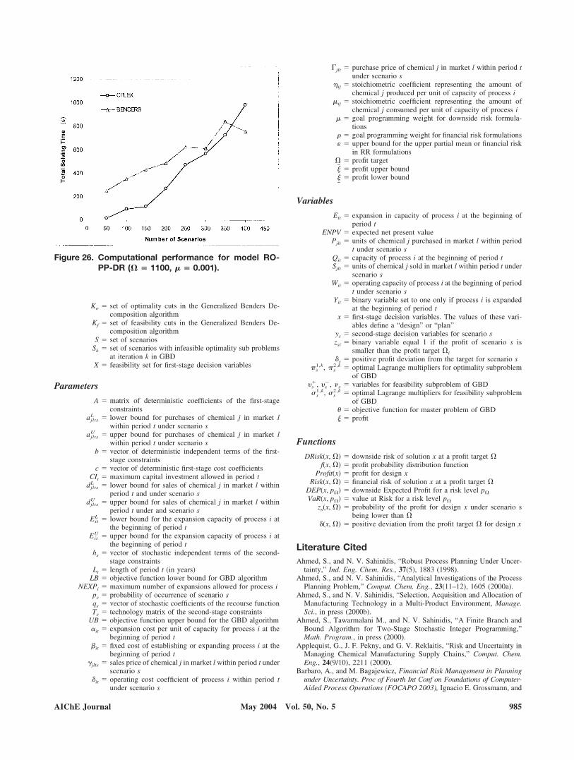
Ko � set of optimality cuts in the Generalized Benders De-composition algorithm

Kf � set of feasibility cuts in the Generalized Benders De-composition algorithm

S � set of scenariosSk � set of scenarios with infeasible optimality sub problems

at iteration k in GBDX � feasibility set for first-stage decision variables

Parameters

A � matrix of deterministic coefficients of the first-stageconstraints

ajltsL � lower bound for purchases of chemical j in market l

within period t under scenario sajlts

U � upper bound for purchases of chemical j in market lwithin period t under scenario s

b � vector of deterministic independent terms of the first-stage constraints

c � vector of deterministic first-stage cost coefficientsCIt � maximum capital investment allowed in period t

djltsL � lower bound for sales of chemical j in market l within

period t and under scenario sdjlts

U � upper bound for sales of chemical j in market l withinperiod t under and scenario s

EitL � lower bound for the expansion capacity of process i at

the beginning of period tEit

U � upper bound for the expansion capacity of process i atthe beginning of period t

hs � vector of stochastic independent terms of the second-stage constraints

Lt � length of period t (in years)LB � objective function lower bound for GBD algorithm

NEXPi � maximum number of expansions allowed for process ips � probability of occurrence of scenario sqs � vector of stochastic coefficients of the recourse functionTs � technology matrix of the second-stage constraints

UB � objective function upper bound for the GBD algorithm�it � expansion cost per unit of capacity for process i at the

beginning of period t�it � fixed cost of establishing or expanding process i at the

beginning of period t�jlts � sales price of chemical j in market l within period t under

scenario sit � operating cost coefficient of process i within period t

under scenario s

�jlt � purchase price of chemical j in market l within period tunder scenario s

�ij � stoichiometric coefficient representing the amount ofchemical j produced per unit of capacity of process i

ij � stoichiometric coefficient representing the amount ofchemical j consumed per unit of capacity of process i

� goal programming weight for downside risk formula-tions

� � goal programming weight for financial risk formulations� � upper bound for the upper partial mean or financial risk

in RR formulations� � profit target�� profit upper bound

�� profit lower bound

Variables

Eit � expansion in capacity of process i at the beginning ofperiod t

ENPV � expected net present valuePjlt � units of chemical j purchased in market l within period

t under scenario sQit � capacity of process i at the beginning of period tSjlt � units of chemical j sold in market l within period t under

scenario sWit � operating capacity of process i at the beginning of period

t under scenario sYit � binary variable set to one only if process i is expanded

at the beginning of period tx � first-stage decision variables. The values of these vari-

ables define a “design” or “plan”ys � second-stage decision variables for scenario szsi � binary variable equal 1 if the profit of scenario s is

smaller than the profit target �i

s � positive profit deviation from the target for scenario s�s

1,k, �s2,k � optimal Lagrange multipliers for optimality subproblem

of GBD�s

�, �s, �s � variables for feasibility subproblem of GBD

s1,k, s

2,k � optimal Lagrange multipliers for feasibility subproblemof GBD

� � objective function for master problem of GBD� � profit

Functions

DRisk(x, �) � downside risk of solution x at a profit target �f(x, �) � profit probability distribution function

Profit(x) � profit for design xRisk(x, �) � financial risk of solution x at a profit target �

DEP(x, p�) � downside Expected Profit for a risk level p�

VaR(x, p�) � value at Risk for a risk level p�

zs(x, �) � probability of the profit for design x under scenario sbeing lower than �

(x, �) � positive deviation from the profit target � for design x

Literature CitedAhmed, S., and N. V. Sahinidis, “Robust Process Planning Under Uncer-

tainty,” Ind. Eng. Chem. Res., 37(5), 1883 (1998).Ahmed, S., and N. V. Sahinidis, “Analytical Investigations of the Process

Planning Problem,” Comput. Chem. Eng., 23(11–12), 1605 (2000a).Ahmed, S., and N. V. Sahinidis, “Selection, Acquisition and Allocation of

Manufacturing Technology in a Multi-Product Environment, Manage.Sci., in press (2000b).

Ahmed, S., Tawarmalani M., and N. V. Sahinidis, “A Finite Branch andBound Algorithm for Two-Stage Stochastic Integer Programming,”Math. Program., in press (2000).

Applequist, G., J. F. Pekny, and G. V. Reklaitis, “Risk and Uncertainty inManaging Chemical Manufacturing Supply Chains,” Comput. Chem.Eng., 24(9/10), 2211 (2000).

Barbaro, A., and M. Bagajewicz, Financial Risk Management in Planningunder Uncertainty. Proc of Fourth Int Conf on Foundations of Computer-Aided Process Operations (FOCAPO 2003), Ignacio E. Grossmann, and

Figure 26. Computational performance for model RO-PP-DR (� � 1100, � � 0.001).


Conor M. McDonald, eds, ISBN-0965589110, Coral Springs, FL (Jan.,2003).

Beale, E. M. L., “On Minimizing a Convex Function Subject to LinearInequalities,” J. Royal Stat. Soc., Series B 17, 173 (1955).

Bellman, R., and L. A. Zadeh, “Decision-making in a Fuzzy Environment,”Manage. Sci., 17, 141 (1970).

Benders, J. F., “Partitioning Procedures for Solving Mixed-Variables Pro-gramming Problems,” Numerische Mathematik, 4, 238 (1962).

Berman, O., and Z. Ganz, “The Capacity Expansion Problem in the ServiceIndustry,” Comput. Operations Res., 21, 557 (1994).

Birge, J. R., and Louveaux F., Introduction to Stochastic Programming,Springer-Verlag, New York (1997).

Brooke, A., D. Kendrick, and A. Meeraus, GAMS—A User’s Guide, TheScientific Press, Redwood City, CA (1988).

Caroe, C. C, and R. Schultz, “Dual Decomposition in Stochastic IntegerProgramming,” Operations Res. Lett., 24, 37-45 (1999).

Charnes, A., and W. W. Cooper, “Chance-Constrained Programming,”Manage. Sci., 6, 73 (1959).

Cheng, L., E. Subrahmanian, and A. W. Westerberg, “Design and Planningunder Uncertainty: Issues on Problem Formulation and Solution,” Com-put. Chem. Eng., 27(6), 781 (2003).

Cheung, R. K. M., and W. B. Powel, “Shape—A Stochastic HybridApproximation Procedure for Two-Stage Stochastic Programs,” Oper-ations Res., 48(1), 73 (2000).

CPLEX. CPLEX 7.0 User’s Manual. ILOG CPLEX Division. InclineVillage, NV (2000).

Dantzig, G. B., “Linear Programming under Uncertainty,” Manage. Sci., 1,197 (1955).

Dupacova, J., and W. Romisch, “Quantitative Stability for Scenario-BasedStochastic Programs,” Prague Stochastics, 98, S. 119, JCMF, Praha(1998).

Eppen, G. D., Martin R. K., and L. Schrage, “A Scenario Approach toCapacity Planning,” Operations Res., 37, 517 (1989).

Geoffrion, A. M., “Generalized Benders Decomposition,” J. OptimizationTheory Appl., 10, 237 (1972).

Guldimann, T., “The Story of Risk Metrics,” Risk, 13(1), 56 (2000).Gupta, A., and C. Maranas. “Market-Based Pollution Abatement Strate-

gies: Risk Management Using Emission Option Contracts,” Ind. Eng.Chem. Res., 42, 802 (2003).

Higle, J. L., and S. Sen, Stochastic Decomposition. A Statistical Method forLarge Scale Stochastic Linear Programming, Kluwer Academic Pub-lishers, Norwell, MA (1996).

Ierapetritou, M. G., and E. N. Pistikopoulos, “Simultaneous Incorporationof Flexibility and Economic Risk in Operational Planning under Uncer-tainty,” Comput. Chem. Eng., 18(3), 163 (1994).

Infanger, G., “Monte Carlo (Importance) Sampling within a Benders De-composition Algorithm for Stochastic Linear Programs (Extended Ver-sion: Including Results of Large-Scale Problems),” Technical ReportSOL 91-6, Systems Optimization Laboratory, Stanford University, CA(1991).

Infanger, G., Planning under Uncertainty: Solving Large-Scale StochasticLinear Programs, Boyd and Fraser, Danvers, MA (1994).

Iyer, R. R., and I. E. Grossmann, “A Bilevel Decomposition Algorithm forLong-Range Planning of Process Networks,” Ind. Eng. Chem. Res., 37,474 (1998).

Jorion, P., Value at Risk. The New Benchmark for Managing FinancialRisk, 2nd Edition, McGraw Hill, New York (2000).

Kall, P., and S. W. Wallace, Stochastic Programming, Wiley, Chichester,UK (1994).

Linsmeier, T. J., and N. D. Pearson, “Value at Risk,” Financial Analysts J.,56(2), March/April (2000).

Liu, M. L., and N. V. Sahinidis, “Optimization in Process Planning underUncertainty,” Ind. Eng. Chem. Res., 35, 4154 (1996).

Marti, K., and P. Kall, eds., Stochastic Programming Methods and Tech-nical Applications, LNEMS, Vol. 458, Springer-Verlag, Berlin-Heidel-berg (1998).

McCray, A. W. Petroleum Evaluations and Economic Decisions, PrenticeHall, Englewood Cliffs, NJ (1975).

Mulvey, J. M., R. J. Vanderbei, and S. A. Zenios, “Robust Optimization ofLarge-Scale Systems,” Operations Res., 43, 264 (1995).

Murphy, F. H., S. Sen, and A. L. Soyster, “Electric Utility ExpansionPlanning in the Presence of Existing Capacity: A Nondifferentiable,Convex Programming Approach,” Comput. Operations Res., 14, 19(1987).

Pistikopoulos, E. N., and M. G. Ierapetritou, “Novel Approach for OptimalProcess Design under Uncertainty,” Comput. Chem. Eng., 19(10), 1089(1995).

Sahinidis, N. V., I. E. Grossmann, R. E. Fornari, and M. Chathrathi,“Optimization Model for Long Range Planning in the Chemical Indus-try,” Comput. Chem. Eng., 13, 1049 (1989).

Takriti, S., and S. Ahmed, “On Robust Optimization of Two-Stage Sys-tems,” Mathematical Programming, On-line Publication. DOI 10.1007/s10107-003-0373-y (2001).

Uryasev, S., and P. M. Pardalos, eds., Stochastic Optimization: Algorithmand Applications, Kluwer Academic, Norwell, MA (2001).

Verweij, B., S. Ahmed, A. J. Kleywegt, G. Nemhauser, and A. Shapiro,“The Sample Average Approximation Method Applied to StochasticRouting Problems: A Computational Study,” Comput. Appl. Optimiza-tion, 24, 289 (2003).

Zimmermann, H. J., Fuzzy Sets and Decision Making, and Expert Systems,Kluwer Academic Publishers, Boston (1987).

Appendix

A. Continuous behavior of the cumulative risk curves

This appendix proves formally that, if Profit(x) has a con-tinuous probability distribution, then, when the number ofscenarios becomes increasingly large [Cardinality(S)3 ], thecumulative risk curves calculated using scenarios approachcontinuous behavior.

Mathematically, the mentioned observation comes from thefact that the continuous and discrete definitions of financial riskyield the same value, that is

limCard�S�3

�s

pszs�x, ��

�

f�x, ��d� (A1)

Using the definition of risk, one can relate the probabilitydistribution function f (x, �) with a probability as follows

Risk�x, �� P��

�

f�x, ��d� (A2)

Now assume that one takes NS random samples of theuncertainty space using the probability distributions of theuncertain parameters for the problem. Then, each sample sconstitutes a possible scenario with a probability of occurrencedefined as ps � 1/NS, rendering ¥s�S ps � 1.

From probability theory, it is well known that when thenumber of samples (scenarios) becomes increasingly large, thesample distribution approximates the actual distribution of theoriginal probability space. Then, the profit distribution obtainedusing the sampled parameters will approximate to the actualprofit distribution.

Assume now that one has solved the two-stage stochasticproblem with NS scenarios obtaining the resulting profit foreach scenario, �s, among which there are N different values,with N � NS. Afterward, the scenarios were sorted in ascend-ing profit order such that �n�1 � �n for n � 1 to N. In turn, thetotal number of scenarios having a profit less or equal than thetarget � is denoted as N�. Because of the convergence of thesample distribution to the actual distribution of the uncertaintyspace, it follows that when the profit has a continuous proba-bility distribution and NS3 , then N3 , N�3 , and thedifference ��n � �n�1 �n tends to zero.


Now, given that f (x, �) is a continuous function, the MeanValue Theorem may be used to approximate its value at anygiven value of profit �. Then, from Eq. A2, one obtains

f� x, �n� � limNS3

P�� n�1� � P�� n�

��n�1 � �n�(A3)

From probability theory, it follows that the numerator on theright-hand side of Eq. A3 is just the probability of the profitbeing between �n and �n�1 [i.e., P(�n � � � �n�1)]. Using thisresult, the integral defining financial risk in Eq. A2 becomes

�

�

f� x, ��d� � limNS3

�n�1

N� �P��n � � � �n�1�

��n��n

� limNS3

�n�1

N�

P��n � � � �n�1� (A4)

In order to calculate the probability P(�n � � � �n�1), wedefine the set �n as follows: �n � {s �n � �s � �n}. Then

P��n � � � �n�1� � limNS3

Card��n�

NS(A5)

In turn, the cardinality of the set �n can be calculated usingbinary numbers for each scenario, as follows

�sn � �1 If �s � �n

0 otherwise � s � S, 1 � n � N (A6)

Then,

Card��n� � �s

��s,n�1 � �s,n� (A7)

Using this result together with Eq. A5 and the definition ofps, Eq. A4 becomes

�

�


�n�1

N� �s

ps��s,n�1 � �s,n�

� limNS3

�s

ps �n�1

N�

��s,n�1 � �s,n� (A8)

Now the possible values for the last summation in the aboveequation are

�n�1

N�

��s,n�1 � �s,n� � �1 If �s � �0 otherwise � s � S (A9)

Notice that Eq. A9 coincides with the definition of zs givenin Eq. 10. Then, using this observation to replace the lastsummation into Eq. A8 the result sought is finally achieved

�

�


�s

pszs (A10)

B. Relation between expected profit and financial riskfor scenario-based cases

This appendix derives the relationship between expectedprofit and financial risk for the case where the profit has adiscrete probability distribution obtained from a finite numberof scenarios. Assume that the two-stage stochastic problemwith NS scenarios is solved obtaining the resulting profit foreach scenario, �s. Therefore, the expected value of the profitand the financial risk are given by


ps�s (B1)


pszs�x, �� (B2)

Afterward, the scenarios were sorted in ascending profitorder, such that �s�1 � �s. Additionally, for the last scenario[the one with the highest profit and Ordinal(s) � NS] �NS�1 isdefined as �� , with �� being any value larger than �NS. Similarly,�� is defined as the lowest scenario profit [Ordinal(s) � 1].Using these definitions, the incurred financial risk at a profit �s

can be expressed as

Risk��x, �s� � Risk��x, �s1� � ps (B3)

Here, the superscript “�” stands for the limit coming from theright, given that in the scenario-based cases Risk(x, �) is adiscontinuous step-shaped function at �s for all s � S. Solvingfor ps and replacing in Eq. B1 yields


Ord�s��1

�Risk��x, �s� � Risk��x, �s1��s

� Risk��x,��

�� (B4)

By distributing the summations and rearranging, this lastexpression becomes


Ord�s��1

Risk��x, �s��s � Risk��x,��

��

� �s�S

Ord�s��1

Risk��x, �s1��s (B5)

Notice that the term between parentheses in Eq. B5 is equal to�s�S Risk�(x, �s)�s. In turn, the last term can be written as

�s�S

Ord�s��NS

Risk��x, �s��s�1

or simply


�s�S

Risk��x, �s��s�1 � ��

Finally, using these expressions in Eq. B5, the relationshipsought is obtained:


Risk��x, �s��s�1 � �s� (87)

The summation in this expression represents the area underthe cumulative risk curve, as illustrated in Figure 8.

C. Behavior of the risk curves

Theorem 1 Let x* denote the optimal values of the first-stagevariables for problem SP and x the values of first-stage vari-ables for any other feasible solution with E[Profit(x)] �E[Profit(x*)] and E[Profit(x*)] � . Then, there exists � � �such that Risk(x, �) � Risk(x*, �).

Proof: The proof is by contradiction. Consider the case wherethe profit has a continuous probability distribution, given thatthe discrete distribution case can be seen as a particular case ofthe former. Assume that there exists a solution x for whichRisk(x, �) � Risk(x*, �) @ � � �. Then, the strategy is toshow that this yields E[Profit(x)] � E[Profit(x*)], which isimpossible because x* is the optimal solution to model SP.Under these assumptions

Risk�x, ��

�

f�x, ��d� (C1)

Risk�x*, ��

�

f�x*, ��d� (C2)

E�Profit�x�� lim�3

��

�

�f�x, ��d� � lim�3

�Risk� x,��

Risk� x,��

�dRisk�x, ��

(C3)

E�Profit�x*�� lim�3

��

�

�f�x*, ��d�

� lim�3

�Risk� x*,��

Risk� x*,��

�dRisk�x*, �� (C4)

Integrating by parts, the expected values can be rewritten as

E�Profit�x�� lim�3

��Risk�x, ��

�

�

Risk�x, ��d�� (C5)

E�Profit�x*�� lim�3

��Risk�x*, ��

�

�

Risk�x*, ��d��(C6)

The difference between the expected values is

E�Profit�x*�� E�Profit�x�� lim�3

��Risk�x*, ��

� Risk�x, ��

�

�

�Risk�x, �� Risk�x*, ��d�� (C7)

The first term in the righthand side of Eq. C7 vanishes, giventhat Risk(x*, �) � Risk(x, �) � 1 and Risk(x*, �) � Risk(x,�) � 0 for some sufficiently large value of �. In addition,because of the assumption that Risk(x, �) � Risk(x*, �) @ � ��, the integrand in the second term is negative @ � � �. Thus,one arrives at E[Profit(x)] � E[Profit(x*)], which is the con-tradiction sought.

Corollary 1 It is impossible to obtain a feasible design xhaving a risk curve that lies entirely below the risk curve of theoptimal design of problem SP.

D. Equivalence of models RO-SP-FR and RR-SO-FR

Theorem 2 For a given �i � 0, (x*, y*, z*) is an optimalsolution of problem RR-SP-FR if and only if there exist �i � 0such that (x*, y*, z*) is an optimal solution of problem RO-SP-FR.

Proof: The approach for this proof was first presented inAhmed and Sahinidis (1998), applied to the robustness formu-lations. Consider the following Lagrangian relaxation (LR) ofproblem RR-SP-FR where constraints 35 are relaxed and �i arethe corresponding Lagrange multipliers.

LR

Max �s�S


i�I

�i��s�S

pszsi � �i (88)


Because the set of constraints 35 is convex, the strongduality theorem proves that a solution (x*, y*, z*) is optimal toRR-SP-FR if and only if it is optimal to the above relaxedproblem (LR) with �i � 0. The proof follows by realizing thatRO-SP-FR is equivalent to LR for positive �i.

E. Pareto optimality of the solutions of riskmanagement models

Theorem 3 An optimal solution to models RO-SP-FR andRR-SP-FR is not stochastically dominated by any other solu-tion; that is, the solution is Pareto optimal.


Proof: Assume solution I to be an optimal solution to modelRR-SP-FR. Furthermore, assume I is stochastically dominatedby another feasible solution II. Then, by definition of stochasticdominance, II has an expected profit strictly greater than that ofI. However, this contradicts the assumption that solution I isoptimal. Thus, an optimal solution to RR-SP-FR cannot bestochastically dominated by any other solution. The proof formodel RO-SP-FR follows from the equivalence derived inTheorem 2.

F. Feasible region of problems SP and RO-SP-FR

Theorem 4 Any first-stage solution x that is feasible for prob-lem SP with Profit(x) � , is also feasible in problem RO-SP-FR; that is, the problems have the same feasible region.

Proof: Clearly, if solution x is feasible in problem SP it mustsatisfy constraints 2 to 5, which are also present in problemRO-SP-FR. In addition, constraints 30 to 32 are satisfied forany value of x provided Us is a valid profit upper bound.Consequently, all constraints of problem RO-SP-FR are satis-fied and, thus, x is feasible in RO-SP-FR. Then, if everyfeasible solution to problem SP is also feasible in problemRO-SP-FR, it follows that the feasible region of the latterincludes the feasible region of the former. In turn, any feasiblesolution of problem RO-SP-FR has to satisfy constraints 2 to 5and is therefore feasible in SP. From this it follows that bothfeasible regions are equal.

Manuscript received Aug. 19, 2003, and revision received Aug. 21, 2003.


Managing financial risk in planning under uncertainty - ResearchGate

Documents

Transcript of Managing financial risk in planning under uncertainty - ResearchGate