Managing Con⁄icts in Relational Contracts · The Lincoln Electric Company provides an example of...

Managing Con�icts in Relational Contracts�

Jin Liy Niko Matouschekz

Northwestern University Northwestern University

December 2012

Abstract

A manager and a worker are in an in�nitely repeated relationship in which the manager privatelyobserves her opportunity costs of paying the worker. We show that the optimal relationalcontract generates periodic con�icts during which e¤ort and expected pro�ts decline graduallybut recover instantaneously. To manage a con�ict, the manager uses a combination of informalpromises and formal commitments that evolves with the duration of the con�ict. Finally, weshow that liquidity constraints limit the manager�s ability to manage con�icts but may alsoinduce the worker to respond to a con�ict by providing more e¤ort rather than less.

Keywords: relational contracts, imperfect monitoring

JEL classi�cations: C73, D23, D82, J33

�An earlier version of this paper circulated under the title "The Burden of Past Promises." We thank the editorLarry Samuelson and three anonymous referees for their comments and suggestions. We are also grateful to MajaButovich, Anne Duchene, Florian Ederer, Matthias Fahn, Yuk-Fai Fong, Bob Gibbons, Marina Halac, Tom Hubbard,Ed Lazear, Arijit Mukherjee, Mike Powell, Michael Raith, Takuro Yamashita, and Pierre Yared for discussions andconversations. Finally, we thank seminar and conference participants at the ASSA meeting, Chinese Universityof Hong Kong, Columbia, Cornell, CSIO/IDEI Conference on Industrial Organization, Harvard/MIT, IIOC, IIT,National University of Singapore, NBER, Peking University, Queen�s, Shanghai University of Finance and Economics,Utah Winter Business Economics Conference, and the 8th Workshop on Industrial Organization and ManagementStrategy. All remaining errors are of course our own.

yKellogg School of Management, [email protected] School of Management, [email protected].

1 Introduction

Relational contracts often su¤er from con�icts during which workers punish managers for broken

promises. A common cause for such con�icts is disagreement over the availability and e¢ cient use

of funds. In a typical con�ict of this sort, workers demand that a bonus be paid while managers

insist that the necessary funds are either non-existent or would be better spent on something else,

such as an exceptional investment opportunity.

One source of disagreement over the availability and e¢ cient use of funds is asymmetric in-

formation. Managers are typically better informed about the challenges and opportunities that

their �rms face and therefore often have private information about the opportunity costs of paying

their workers. The aim of this paper is to explore optimal relational contracts in such a setting.

For this purpose, we examine the repeated relationship between a manager and a worker in which

the manager�s opportunity costs of paying the worker are stochastic and privately observed by

her. In the optimal relational contract, the manager promises a bonus if opportunity costs are

low but none if they are high. Con�icts therefore arise whenever the manager does not pay the

bonus. To manage these con�icts, the manager relies on a combination of informal promises and

formal commitments that evolves with the duration of the con�ict. As a result, e¤ort and expected

pro�ts decline during a con�ict only gradually and then recover instantaneously. The same pat-

tern is repeated over time. The relationship between the manager and the worker therefore never

terminates, nor does it reach a steady state. Instead, it cycles inde�nitely.

The Lincoln Electric Company provides an example of the type of situation that motivates this

paper. In the early 1990s, Lincoln Electric was a leading manufacturer of welding machines, well-

known for its promise to share a signi�cant fraction of pro�ts with its factory workers. In 1992,

Lincoln�s U.S. business had generated a signi�cant pro�t and as a result its U.S. workers expected

to be paid their bonus. Mounting losses in its recently acquired foreign operations, however, more

than wiped out U.S. pro�ts. This presented CEO Donald Hastings with a dilemma: �Our 3,000

U.S. workers would expect to receive, as a group, more than $50 million. If we were in default, we

might not be able to pay them. But if we didn�t pay the bonus, the whole company might unravel�

(Hastings 1999, p.164). To prevent the company from unraveling, Hastings decided to borrow

$52.1 million and pay the bonus.

Why would Hastings have to take the seemingly ine¢ cient step of borrowing money to pay

the bonus? After all, the bonus was explicitly a �cash-sharing bonus� and U.S. workers had a

long history of accepting �uctuations in the bonus in response to �uctuations in U.S. pro�ts. The

reason, it seems, was that U.S. workers were unable to observe foreign losses and therefore did not

1

know whether U.S. pro�ts really were needed to cover those losses. This explains why shortly after

he paid the bonus, Hastings �[...] instituted a �nancial education program so that employees would

understand that no money was being hidden from them [...]�(Hastings 1999, p.172).

The Lincoln Electric case illustrates the issues that arise if a manager is privately informed

about the opportunity costs of paying her worker. In such a setting, if the manager does not pay

a bonus, the worker cannot observe her motives. Is the manager not paying the bonus because it

is more e¢ cient to spend resources on something else, as she claims? Or is she just making up an

excuse to extract some of the worker�s rents? To keep the manager honest, the worker must then

punish her whenever she does not pay a bonus. As a result, the manager faces a trade-o¤ between

the current bene�ts of adapting bonus payments to their opportunity costs and the future costs the

worker in�icts on her if she does not pay a bonus. In short, the manager faces a trade-o¤ between

the bene�ts of adaptation and the costs of con�ict.

To explore this trade-o¤, we examine a �rm that consists of a risk-neutral owner-manager

and a risk-neutral but liquidity-constrained worker. Output and e¤ort are observable but not

contractible. At the beginning of every period the manager o¤ers the worker a contractible wage

and a non-contractible bonus. After accepting the o¤er, the worker decides on his e¤ort level.

E¤ort is continuous and imposes a cost on the worker. Finally, output is realized and the manager

decides how much to pay the worker. So far this is a relational contracting model with public

information that is well understood (MacLeod and Malcomson 1989). The only change we make

to this standard model is to assume that the manager�s opportunity costs of paying the worker

are stochastic and privately observed by her. In particular, just before the manager decides how

much to pay the worker, she observes whether the �rm has been hit by a shock� in which case

opportunity costs are high� or not� in which case they are low.

In this setting, it is optimal for the manager to motivate the worker by promising to pay

him a bonus. The bonus, however, is contingent on opportunity costs being low. To keep

the manager honest, the worker punishes her when she does not pay a bonus and rewards her

when she does. In particular, if the manager does not pay the bonus this period, expected

pro�ts will be lower next period, unless they are already at their lower bound, in which case

they stay there. In contrast, expected pro�ts immediately jump to their upper bound if the

manager does pay the bonus. Expected pro�ts therefore cycle inde�nitely and the relationship

never terminates. These cycles di¤er in length depending on the number of consecutive shock

periods the �rm experiences. They all, however, follow the same pattern in which downturns are

gradual and recoveries instantaneous. In our setting, it is therefore not optimal for the parties

2

to alternate between high pro�t �cooperation�phases and low pro�t �punishment�phases, as in

Green and Porter (1984). Nor is it optimal for them to adopt termination contracts in which the

failure to pay the bonus triggers the termination of their relationship with some probability, as in

Levin (2003).

One reason for why downturns are gradual and recoveries instantaneous is that joint surplus is

increasing in expected pro�ts. Essentially, the larger is the manager�s stake in the relationship, the

less tempted she is to renege, and thus the more e¤ort the worker is willing to provide. Rewarding

the manager for paying a bonus is therefore not only good for her incentives to act truthfully but

is also e¢ ciency enhancing. As a result, it is optimal for expected pro�ts to jump to their upper

bound when the manager pays the bonus. In contrast, punishing the manager for not paying the

bonus destroys joint surplus. Since the production function is concave, the most e¢ cient way to

punish the manager is then to reduce pro�ts gradually.

To see how the optimal punishment is implemented, consider a period in which expected pro�ts

are not at their lower bound and suppose the manager does not pay the bonus. In the next period,

the manager will then have to o¤er the worker a larger bonus. Moreover, the manager will either

have to accept a reduction in e¤ort or o¤er a higher wage. In particular, the optimal punishment

calls for a reduction in e¤ort if expected pro�ts are high and an increase in the wage if they are

low. The reason for this pattern is again the concavity of the production function, which makes it

more e¢ cient to punish the manager through a reduction in e¤ort if expected pro�ts are high and

through an increase in wages if they are low.

The optimal punishment gives rise to con�icts that go through up to three distinct phases.

Initially, the manager responds to a con�ict by o¤ering the worker a larger and larger bonus but

she does not commit to a wage. In response, the worker provides less and less e¤ort. Once

expected pro�ts are su¢ ciently low, the con�ict enters its second phase during which the manager

complements his promise to pay larger and larger bonuses with the formal commitment to also

pay higher and higher wages. In response, the worker no longer reduces e¤ort. Finally, expected

pro�ts reach their lower bound and the con�ict enters its �nal phase. During this phase the bonus

and the wage stay constant at their maximized levels and the worker continues to provide the same

level of e¤ort. The �nal phase of the con�ict continues until a period in which the �rm is not hit

by a shock, at which point the con�ict ends and expected pro�ts return to their upper bound.

A key assumption in our model is that the �rm is not liquidity-constrained. The manager can

therefore always pay the worker any positive amount, even if the opportunity costs of doing so may

be high. In our main extension we relax this assumption. We show that liquidity constraints

3

limit the manager�s ability to manage con�icts, which slows down recoveries and may lead to

termination. They can also, however, induce the worker to respond to a con�ict by providing

more e¤ort rather than less. Essentially, the worker understands that more e¤ort relaxes the �rm�s

liquidity constraint, which, in turn, allows the manager to pay him a larger bonus.

To illustrate the role of liquidity constraints in managing relational contracts, we return to the

Lincoln Electric case. In early 1993, a few months after he had borrowed the necessary funds

to pay his workers, CEO Hastings realized that European losses would once again wipe out U.S.

pro�ts. The covenants in the debt that he took on the previous year, however, prevented him from

again borrowing the necessary funds to pay the bonus:

�[...] we turned to our U.S. employees for help. I presented a 21-point plan to the board that

called for our U.S. factories to boost production dramatically [...]. �We blew it,�I said [to the U.S.

employees]. �Now we need you to bail the company out. If we violate the covenants, banks won�t

lend us money. And if they don�t lend us money, there will be no bonus in December��(Hastings

1999, pp.171-172).

According to Hastings, his �statement appealed not only to [the U.S. workers�] loyalty but also

to what James F. Lincoln called their �intelligent sel�shness�� (Hastings 1999, p.172). And,

apparently, it worked:

�Thanks to the Herculean e¤ort in the factories and in the �eld, we were able to increase

revenues and pro�ts enough in the United States to avoid violating our loan covenants�(Hastings

1999, p.178).

As a result, Hastings was able to renew the covenants, which, in turn, allowed him to once again

borrow the necessary funds and pay the bonus. In line with the reasoning that we sketched above,

therefore, Lincoln Electric�s U.S. workers increased their e¤orts so as to relax the �rm�s liquidity

constraints, which, in turn, ensured that they were paid their bonus.

2 Related Literature

There is a large literature that examines relational contracts both between and within �rms; see

MacLeod (2007) and Malcomson (forthcoming) for recent reviews. Our paper contributes to the

branch of this literature that studies the actions managers can take to sustain relational contracts

better, such as the timing of payments (MacLeod and Malcomson 1998), the design of explicit

contracts (Baker, Gibbons, and Murphy 1994, Che and Yoo 2001), the allocation of ownership

rights (Baker, Gibbons, and Murphy 2002, Rayo 2007), the di¤erential treatment of workers (Levin

2002), the grouping of tasks (Mukherjee and Vasconcelos 2011), and others. In contrast to these

4

papers, our focus is on how to manage con�icts once they arise, rather than on how to prevent

them in the �rst place.

Our paper contributes to the branch of the literature on relational contracts in which the

manager is privately informed about aspects of the relationship. In this context, three closely

related papers are Levin (2003), Fuchs (2007), and Englmaier and Segal (2011). In the second

part of Levin (2003), the manager privately observes the worker�s performance. In contrast to

our setting, the worker�s e¤ort is privately observed, which makes joint punishments necessary.

Levin shows that the optimal contract is stationary and can be implemented through a termination

contract. In the same setting, Fuchs (2007) allows for private monitoring and shows that while the

optimal contract can still be implemented through a termination contract, it is no longer stationary.

In both models e¢ cient transfers are always available. In contrast, in our setting e¢ cient transfers

are not always available and as a result termination contracts are not optimal.

Englmaier and Segal (2011) correspond to a version of our model in which e¤ort is binary and

the manager�s opportunity costs in a shock period are in�nite. They focus on a particular relational

contract in which the parties alternate between phases with high and low e¤ort. In contrast, we

characterize the optimal relational contract and show that under such a contract con�icts evolve

more gradually.

Another closely related paper, albeit in a di¤erent context, is Yared (2010). He characterizes

the optimal sequential equilibria in a game between an aggressive country that demands transfers

from a peaceful one, where the peaceful country is privately informed about the costs of paying the

transfers. In this setting, the aggressive country can punish the peaceful one through the binary

choice of going to war or not. In contrast, in our setting the worker can punish the manager

by providing less e¤ort or demanding higher wages, both of which are continuous choices. As a

result, optimal temporary con�icts are more gradual in our setting than optimal temporary wars

in Yared�s paper. Moreover, while in his setting the parties eventually engage in permanent war,

termination is never optimal in ours.

Our paper also contributes to the recent and growing literature on dynamics within relational

contracts. Chassang (2010) studies a model of exploration with private information and shows

that the relationship is path-dependent and can settle in di¤erent long-run equilibria. Fong and Li

(2010) study a moral hazard problem in which the worker has limited liability and explore patterns

of the worker�s job security, pay level, and the sensitivity of pay to performance. Padro i Miquel and

Yared (2011) examine a political economy model and study the likelihood, duration, and intensity

of war. Thomas and Worrall (2010) examine a partnership game with perfect information and

5

two-sided limited liability. They show that the relationship becomes more e¢ cient over time as the

division of future rents becomes more equal. Dynamics also arise in models of relational contracts

in which agents have private and �xed types; see, for example, Halac (forthcoming), Watson (1999,

2002), and Yang (2011). In these papers, dynamics arise when the principal updates her beliefs

about the agent�s type.

In terms of its analytical structure, our model is related to the literature on dynamic games

with hidden information; see, for example, Abdulkadiroglu and Bagwell (2010), Athey and Bagwell

(2001, 2008), Athey, Bagwell and Sanchirico (2004), Hauser and Hopenhayn (2008), Mobius (2001),

and for surveys, Mailath and Samuelson (2006) and Samuelson (2006). A distinct feature of our

model is the occasional availability of e¢ cient transfers. As a result, the dynamics in our model

feature gradual downturns or instantaneous recoveries.

Our model is also related to the literature on dynamic contracting between banks and privately

informed entrepreneurs (DeMarzo and Fishman 2007, DeMarzo and Sannikov 2006, Biais et al.

2007, and Clementi and Hopenhayn 2006). In contrast to this literature, we focus on a setting in

which long-term contracts are not feasible. The unavailability of long-term contracts is crucial for

our results. In particular, we show in Section 7 that if the long-term contracts were feasible, the

parties could approximate �rst-best.

Finally, since the e¢ ciency of transfers depends on the state of the world, our model is related

to the large literature on risk sharing. Kocherlakota (1996) and Ligon, Thomas, and Worrall (2002)

explore e¢ cient risk sharing between risk-averse agents when information is public and commit-

ment is limited. Hertel (2004) examines the case with two-sided asymmetric information without

commitment. Thomas and Worrall (1990) study a one-sided asymmetric information problem with

commitment. This literature typically assumes that the player�s endowments are exogenously given

and path-independent. In our model, instead, output depends on the worker�s e¤ort and thus on

how it was divided in the past.

3 The Model

A �rm consists of a risk-neutral owner-manager and a risk-neutral but liquidity-constrained worker.

The manager and the worker are in an in�nitely repeated relationship. Time is discrete and denoted

by t = f1; 2; :::;1g.At the beginning of any period t the manager makes the worker an o¤er. The o¤er consists of

a contractible commitment to pay wage wt � 0 and a non-contractible promise to pay bonuses bs;tand bn;t, where s and n stand for �shock�and �no-shock.� The worker either accepts the o¤er or

6

rejects it. We denote the worker�s decision by dt, where dt = 0 if he rejects the o¤er and dt = 1 if

he accepts it. If the worker rejects the o¤er, the manager and the worker realize their per-period

outside options � > 0 and u > 0 and time moves on to period t+ 1.

If, instead, the worker accepts the manager�s o¤er, he next decides on his e¤ort level et � 0.

E¤ort is costly to the worker and we denote his e¤ort costs by c(et). The cost function is strictly

increasing and strictly convex with c (0) = c0 (0) = 0 and lime!1 c0(e) = 1. After the worker

provides e¤ort et, the manager realizes output y(et). The output function is strictly increasing

and strictly concave with y (0) = 0. E¤ort et, e¤ort costs c (et), and output y (et) are observable

but not contractible.

After the manager realizes output y(et), she privately observes the state of the world �t 2 fs; ng,where, as mentioned above, s and n stand for �shock� and �no-shock.� The states are drawn

independently across time from a binary distribution. The probability with which a shock state

occurs is given by � 2 (0; 1). The state of the world determines the opportunity cost of paying

the worker: if the �rm is not hit by a shock, paying the worker an amount of w + b costs the

manager w + b; if, instead, the �rm is hit by a shock, paying the worker w + b costs the manager

(1 + �) (w+ b), where � 2 (0;1). We do not model explicitly why opportunity costs may be high.As discussed above, however, managers do sometimes face high opportunity costs of paying their

workers. This may be the case, for instance, because they need to borrow money to make their

payments, as in the Lincoln Electric case.

After the manager observes the state of the world, she pays the worker the wage wt and a bonus

bt � 0. Since the promised bonus is not contractible, the payment bt can be di¤erent from the

promises bn;t and bs;t.

Finally, at the end of period t, the manager and the worker observe the realization xt of a public

randomization device. This allows the players to publicly randomize at the beginning of any period

t + 1 � 2 based on the realization of the public randomization device observed at the end of the

previous period. To allow the players to publicly randomize in period 1, we assume that they can

also observe a realization of the randomization device at the beginning of that period. We denote

this realization by x0. The existence of a public randomization device is a common assumption in

the literature and is made to convexify the set of equilibrium payo¤s. The timing is summarized

in Figure 1.

7

Worker chooseseffort

Manager realizesoutput

Manager decideshow much to pay

Manager observesthe state

Publicrandomization

Manager offersbonuses and wage

Worker acceptsor rejects offer

Worker chooseseffort

Manager realizesoutput

Manager decideshow much to pay

Manager observesthe state

Publicrandomization

Manager offersbonuses and wage

Worker acceptsor rejects offer

Figure 1: Timeline

The manager and the worker share the same discount factor � 2 (0; 1). At the beginning of

any period t, their respective expected payo¤s are therefore given by

�t = (1� �)1X�=t

��tE�d��y (e� )�

�1 + 1f��=sg�

�(w� + b� )

�+ (1� d� )�

�and

ut = (1� �)1X�=t

��tE [d� (w� + b� � c (e� )) + (1� d� )u] .

Note that we multiply the right-hand side of each expression by (1� �) to express pro�ts andpayo¤s as per-period averages.

We follow the literature on imperfect public monitoring and de�ne a �relational contract�as a

pure-strategy Perfect Public Equilibrium (henceforth PPE) in which the manager and the worker

play public strategies and, following every history, the strategies are a Nash Equilibrium. Public

strategies are strategies in which the players condition their actions only on publicly available

information. In particular, the manager�s strategy does not depend on her past private information.

Our restriction to pure strategy is without loss of generality because our game has only one-sided

private information and is therefore a game with the product structure (see, for instance, p.310 in

Mailath and Samuelson (2006)). In this case, there is no need to consider private strategies since

every sequential equilibrium outcome is also a PPE outcome (see, for instance, p.330 in Mailath

and Samuelson (2006)).

Formally, let ht+1 = fw� ; bn;� , bs;� , d� , e� , b� , x�gt�=1 denote the public history at the beginningof any period t + 1 and let Ht+1denote the set of period t + 1 public histories. Note that H1 =

�. A public strategy for the manager is a sequence of functions fWt; Bs;t, Bn;t, Btg1t=1, whereWt : Ht ! [0;1) ; Bs;t : Ht ! [0;1), Bn;t : Ht ! [0;1), and Bt : Ht [ fwt; bs;t, bn;t, dt, et; �tg ![0;1). Similarly, a public strategy for the worker is a sequence of functions fDt, Etg1t=1, whereDt : Ht [ fwt; bs;t, bn;tg ! f0; 1g and Et : Ht [ fwt; bs;t, bn;t, dtg ! [0;1).

We de�ne an �optimal relational contract�as a PPE with payo¤s that are not Pareto-dominated

by any other PPE. Note that when the discount factor is su¢ ciently small, the only relational

8

contract is a trivial one in which the parties always take their outside options � and u. To make

the analysis interesting, we assume that the parties are su¢ ciently patient so that a non-trivial

relational contract exists. A su¢ cient condition for a non-trivial relational contract to exist is

y�eFB

�� (1 + ��)

�c�eFB

�+ u

�� 1� �

�(1 + ��) c

�eFB

�;

where eFB is the �rst-best e¤ort that maximizes y (e)� c (e).

4 Preliminaries

In this section we �rst list the constraints that have to be satis�ed for a payo¤ pair to be in the

PPE payo¤ set. We then consider a relaxed problem that ignores one of these constraints. For

this relaxed problem we characterize properties of the PPE payo¤ set in Section 4.2 and properties

of the optimal relational contract in Section 4.3. These properties of the relaxed problem will then

allow us to characterize the optimal relational contract in Section 5.

4.1 The Constraints

We denote the set of PPE payo¤s by E. Each payo¤ pair (�; u) 2 E is associated with a pro�le ofactions (e; w; bs; bn) and continuation payo¤s (�s; �n; us; un), where �s and �n are the manager�s

continuation payo¤s associated with shock and no-shock states and us and un are de�ned analo-

gously. We say that a PPE payo¤ pair (�; u) can be �supported�by pure actions if there exists

a pro�le of actions (e; w; bs; bn) and continuation payo¤s (�s; �n; us; un) that satisfy the following

three sets of constraints.

Feasibility: For the actions to be feasible, the wage, bonuses, and e¤ort have to be non-negative.

Speci�cally, the non-negativity constraints are given by

w � 0; (NNW)

bn � 0; (NNN)

bs � 0; (NNS)

and

e � 0: (NNe)

Moreover, for the continuation payo¤s to be feasible, they also need to be PPE payo¤s. The

self-enforcing constraints are therefore given by

(�n; un) 2 E (SEN)

9

in a no-shock period and

(�s; us) 2 E (SES)

in a shock period.

No Deviation: To ensure that neither party deviates, we need to consider both o¤- and on-

schedule deviations. O¤-schedule deviations are deviations that can be publicly observed. There

is no loss of generality in assuming that if an o¤-schedule deviation occurs, the parties terminate

their relationship, as this is the worst possible equilibrium that gives each party its minmax payo¤.

The manager deviates o¤-schedule when he pays a bonus that is di¤erent from either bs or bn.

If the manager does deviate o¤-schedule, she cannot do better than to pay a zero bonus. The

non-reneging constraints are therefore given by

��n � �� (1� �) bn (NRN)


��s � �� (1� �) (1 + �) bs (NRS)

in a shock period.

The worker deviates o¤-schedule when he rejects the manager�s o¤er or provides an e¤ort level

that is di¤erent from e. The individual rationality constraint

u � u (IRW)

ensures that the worker does not reject the manager�s o¤er. If the worker accepts the o¤er but

deviates by providing an e¤ort level that is di¤erent from e, he cannot do better than to provide

no e¤ort. The worker�s incentive constraint is therefore given by

u � (1� �)w + �u: (ICW)

In contrast to o¤-schedule deviations, on-schedule deviations are only privately observed. Since

the worker does not have any private information, he cannot engage in any on-schedule deviations.

The manager, however, can do so by either paying bn in a shock period or bs in a no-shock period.

The manager�s truth-telling constraints are therefore given by

� (�n � �s) � (1� �) (bn � bs) (TTN)


� (�n � �s) � (1 + �) (1� �) (bn � bs) (TTS)

in a shock period.

10

Promise Keeping: Finally, the consistency of the PPE payo¤ decomposition requires that the

parties�payo¤s are equal to the weighted sum of current and future payo¤s. The promise-keeping

constraints are therefore given by

� = � f(1� �) [y (e)� (1 + �) (w + bs)] + ��sg+ (1� �) f(1� �) [y (e)� w � bn] + ��ng (PKM)

for the manager and

u = � [(1� �) (w + bs) + �us] + (1� �) [(1� �) (w + bn) + �un]� (1� �) c (e) (PKW)

for the worker.

4.2 Properties of the PPE Payo¤ Set

Before characterizing the optimal relational contract that satis�es all the constraints in the previous

section, we �rst turn to a relaxed problem that ignores the worker�s incentive constraint ICW. To

streamline the exposition, however, we keep the same notation as above.

Speci�cally, we now use the technique developed by Abreu, Pearce, and Stacchetti (1990) to

characterize the PPE payo¤ set E of the relaxed problem. For this purpose, we de�ne the payo¤

frontier as

u(�) � supfu0 : (�; u0) 2 Eg:

Our �rst lemma establishes several properties of the PPE payo¤ set E.

LEMMA 1. The PPE payo¤ set E has the following properties: (i.) it is compact, (ii.) payo¤

pair (�; u) belongs to E if and only if � 2 [�; �] and u 2 [u; u (�)], and (iii.) the extremal pointu(�) satis�es u(�) = u:

A key implication of this lemma is that the PPE payo¤ set E is fully characterized by its frontier

u(�). To see why, notice that for any u(�), the points below it can be sustained by randomizing

among (�; u), (�; u), and (�; u(�)). Since the PPE frontier fully characterizes the PPE payo¤ set,

we now turn to the next lemma, which establishes several of its properties.

LEMMA 2. The PPE frontier u (�) has the following properties: for all � 2 [�; �], (i.) payo¤s(�; u(�)) can be supported by pure actions in the stage game other than taking the outside options,

(ii.) u is concave, and (iii.) u is di¤erentiable with �1 < u0(�) � �1=(1 + ��).

The �rst part of the lemma shows that payo¤s on the PPE frontier can be supported by

pure actions, that is, they do not require any public randomization. This fact will allow us to

represent the PPE frontier recursively below. This property follows from the concavity of the

11

output function y (e). Essentially, any PPE that is supported by randomization between two e¤ort

levels can be improved upon by having the worker provide an appropriately chosen intermediate

level of e¤ort. The concavity of the PPE frontier follows immediately from the availability of a

public randomization device and its di¤erentiability follows from the continuity of e¤ort. Finally,

the bounds on the derivative imply that the PPE frontier is downward sloping and that joint surplus

� + u (�) is increasing in expected pro�ts � and thus maximized at �. Figures 2a and b illustrate

these properties.

πππ

u

u

)(πu

πππ

u

u

)(πu

ππππ

u

u

)(πu

πππ

u

u

)(πu

πππ

u

u

)(πu

π πππ

u

u

)(πu

π

Figures 2a and 2b: The PPE Frontier

In both �gures the PPE frontier is downward sloping and joint surplus is maximized at �. The

di¤erence between the two �gures is that in Figure 2a the derivative of the PPE frontier never

reaches its upper bound u0(�) = �1=(1+��). In Figure 2b, instead, the derivative does reach thisupper bound at a critical level of expected pro�ts b� and as a result the PPE frontier is linear forall � � b�. This critical level of expected pro�ts is de�ned by

b� = (1� �)y(be) + ��; (1)

where be is the unique e¤ort level that solvesc0(be)y0(be) = 1

1 + ��. (2)

12

Notice that b� can be smaller than �, as in Figure 2a, or it can be larger, as in Figure 2b. We willsee in the next section that b� is the threshold level of expected pro�ts below which the managerpays a positive wage and above which the wage is zero.

4.3 Properties of Optimal Relational Contracts

We now turn to properties of the optimal relational contract. We continue to focus on the relaxed

problem that ignores the ICW constraint. The next lemma shows that any optimal relational

contract is sequentially optimal.

LEMMA 3. Any optimal relational contract is sequentially optimal, that is, for any PPE payo¤

pair (�; u(�)), the associated continuation payo¤s satisfy us = u(�s) and un = u(�n).

Essentially, since the worker�s actions are publicly observable, it is not necessary to punish him

by moving below the PPE frontier. This feature of our model is similar, for instance, to Spear and

Srivastava (1987) and the �rst part of Levin (2003). In contrast, joint punishments are necessary

in models with two-sided private information, such as Green and Porter (1984), Athey and Bagwell

(2001), and the second part of Levin (2003).

Recall from Lemma 2 that payo¤s on the frontier are sustained by pure actions. Lemma 3 then

implies that the optimal relational contract does not involve any public randomization. In what

follows we therefore refer to an optimal relational contract as one in which no public randomization

device is used.

Next we can simplify and combine some of the constraints in Section 4.1. In particular, the

next lemma will allow us to eliminate the shock and no-shock bonuses from the above constraints.

LEMMA 4. For any optimal relational contract with payo¤s (�; u(�)), there exists a set of actions

and continuation payo¤s supporting it such that (i.) the bonuses satisfy bn(�) � bs (�) = 0 and

(ii.) the manager�s truth-telling constraint in a no-shock period TTN is binding.

Since it is less expensive for the manager to pay the worker in a no-shock period than in a

shock period, it is natural that bn(�) � bs (�). As a result, one can always replicate a PPE in

which bs (�) > 0 with an economically equivalent one in which the shock bonus is zero. To do so,

one simply has to add bs (�) to the wage and subtract it from the no-shock bonus. Finally, the

fact that TTN is binding follows from the concavity of the PPE frontier u (�). Essentially, if TTN

were not binding, one could always reduce �n and increase �s in such a way that � remains the

same and all the relevant constraints continue to be satis�ed. Since the PPE frontier is concave,

however, such a change would make the worker better o¤.

13

The lemma allows us to eliminate bs (�) from the constraints in Section 4.1 by setting it equal

to zero. Furthermore, we can now eliminate a number of these constraints. For instance, it is

immediate that if TTN is binding, TTS is satis�ed. The next lemma shows that we can represent

the PPE frontier by focusing on only four of the above constraints.

LEMMA 5. The PPE frontier u(�) is recursively de�ned by the following problem. For all

� 2 [�; �],

� + u(�) = maxe;w;�s;�n

(1� �) (y (e)� c (e)) + �� (�s + u (�s)) + (1� �) � (�n + u (�n))� (1� �) ��w

such that

w � 0; (NNW)

� � �n � �; (SEN)

� � �s � �; (SES)

and

� = (1� �) y (e) + ��s � (1� �) (1 + ��)w: (PKM)

Notice that there might be multiple functions u (�) that solve this problem. This type of

multiplicity is common in games of relational contracts (see, for instance, Baker, Gibbons, and

Murphy (1994)). When multiple solutions exist, it is immediate that the PPE frontier is given by

the largest one.

In the next section we characterize the solution to this problem and show that it satis�es the

ICW constraint that we ignored so far. The solution to the problem in the lemma therefore

characterizes the optimal relational contracts for the full problem.

5 The Optimal Relational Contract

In this section we characterize the optimal relational contract. We saw in the previous section that

there is no loss of generality in setting the shock bonus equal to zero. We therefore now de�ne an

optimal relational contract to be a PPE that is not Pareto-dominated by any other PPE and in

which bs = 0. Our �rst proposition characterizes the optimal relational contract and shows that

it is unique. In the proof of the proposition we solve the relaxed problem in Lemma 5 and then

show that it satis�es the ICW constraint that we ignored so far.

PROPOSITION 1. For any level of expected pro�ts �, there exists a unique optimal relational

contract that gives the worker u(�). Under the optimal relational contract:

14

(i.) The no-shock bonus b�n(�) is given by

b�n (�) =�

1� � (� � ��s (�)) > 0 for all � 2 [�; �] .

(ii.) If the �rm is hit by a shock, the continuation pro�t ��s (�) satis�es

��s (�) = � and ��s (�) < � for all � 2 (�; �] :

(iii.) If the �rm is not hit by a shock, the continuation pro�t is given by

��n (�) = � for all � 2 [�; �] :

(iv.) E¤ort e� (�) is given by the unique e¤ort level e that solves

c0(e)

y0(e)= �u0 (�) for all � 2 [�; �] .

(v.) The wage is given by

w� (�) = max� b� � �(1� �)(1 + ��) ; 0

�for all � 2 [�; �] .

The optimal relational contract re�ects a balancing of incentives. In particular, the manager

must give the worker an incentive to provide e¤ort, while the worker must give the manager an

incentive to make any promised payments. Part (i.) shows that the manager motivates the worker

to provide e¤ort by promising him a bonus. The promise, however, is contingent on opportunity

costs being low. The worker must therefore motivate the manager to act truthfully.

To motivate the manager to act truthfully, the worker punishes her if she does not pay the

bonus, and rewards her if she does. In particular, part (ii.) shows that if the manager does not

pay the bonus, expected pro�ts will be strictly lower next period, unless they are already at their

lower bound �, in which case they stay there. In contrast, part (iii.) shows that if the manager

does pay the bonus, expected pro�ts immediately jump to their upper bound � in the next period.

Expected pro�ts therefore cycle inde�nitely and the relationship never terminates. These cycles

di¤er in length depending on the number of consecutive shock periods the �rm experiences. They

all, however, follow the same pattern in which downturns are gradual and recoveries instantaneous.

These dynamics are illustrated in Figure 3 which plots expected pro�ts for an arbitrary sequence

of shock periods� indicated by red squares� and no-shock periods� indicated by blue dots.

15

time0

ππ

π

time0

ππ

π

Figure 3: Evolution of Expected Pro�ts

To understand why downturns are gradual and recoveries are instantaneous, recall that joint

surplus � + u (�) is increasing in expected pro�ts. Rewarding the manager for paying the bonus

is therefore both good for her incentives to act truthfully and e¢ ciency enhancing. As a result, it

is optimal for expected pro�ts to jump to their upper bound if the manager pays the bonus. In

contrast, punishing the manager for not paying the bonus involves a destruction of joint surplus.

In principle, the worker could punish the manager for not paying the bonus by insisting that

expected pro�ts plummet to � in the next period. One way to do so would be to terminate the

relationship. As discussed after Lemma 3, however, termination is not optimal in our setting since

the public observability of the worker�s actions makes joint punishments unnecessary. Another

way to force expected pro�ts to � would be to reduce e¤ort signi�cantly for a number of periods

without, however, terminating the relationship. The dynamics would then be reminiscent of those

in Green and Porter (1984) in which the parties alternate between cooperation and non-cooperation

phases. Because of the concavity of the production function, however, such a punishment is not

optimal in our setting. Instead, the optimal punishment involves changes to the bonus, e¤ort, and

wages that lead to a gradual reduction in expected pro�ts.

Speci�cally, part (i.) shows that the optimal punishment involves an increase in the bonus

that the manager has to pay the worker in the next period. Since the bonus only has to be paid

if opportunity costs turn out to be low, this part of the punishment is e¢ cient. But since the

opportunity costs are only observed by the manager, the optimal punishment must also involve

changes in the wage, e¤ort, or both.

The last two parts of the proposition show that if expected pro�ts are high, the optimal punish-

ment involves a reduction in e¤ort but no change in the wage; and if expected pro�ts are low, the

optimal punishment involves an increase in the wage but no change in e¤ort. To see this formally,

16

recall from Section 4.2 that b� is the critical level of expected pro�ts below which the derivative ofthe PPE frontier is at its upper bound. Part (iv.) then implies that e¤ort is the same for all � � b�and increasing in expected pro�ts for all � > b�. At the same time, part (v.) implies that wages

are decreasing in expected pro�ts for all � � b� and zero for all � > b�. Essentially, because of theconcavity of the production function, there is a threshold level of pro�ts above which it is more

e¢ cient to punish the manager through a reduction in e¤ort and below which it is more e¢ cient

to do so through an increase in the wage.

To see this more clearly, consider two ways in which expected pro�ts can be reduced by some

" > 0. One way to do so is to reduce e¤ort by "=y0 (e) and the other is to increase wages by

"= (1 + ��). The reduction in e¤ort increases the worker�s expected payo¤ by "c0 (e) =y0 (e), while

the increase in wages increases it by "= (1 + ��). Recall now from Section 4.2 that the e¤ort levelbe that is associated with expected pro�ts b� is de�ned by c0 (be) =y0 (be) = 1= (1 + ��). For expectedpro�ts above b� it is therefore more e¢ cient to punish the manager through a reduction in e¤ort,and for expected pro�ts below b� it is more e¢ cient to do so through an increase in the wage.

e

bn

w

0time

Phase 3Phase 2Phase 1


ê

e

bn

w

0time



ê

Figure 4: Evolution of E¤ort, Bonuses, and Wages

17

To illustrate the evolution of bonuses, e¤ort, and wages over time, suppose that expected pro�ts

are at their upper bound � and that the �rm is then hit by shocks in a large number of consecutive

periods. The resulting con�ict goes through three distinct phases, which are illustrated in Figure

4. As in Figure 3, red squares indicate shock periods and blue dots indicate no-shock periods.

In the initial phase of the con�ict, the bonus is increasing and e¤ort is decreasing. Wages,

however, stay constant at zero. Once expected pro�ts fall below b�, the con�ict enters its secondphase. During this phase the bonus is still increasing. Wages, however, are now also increasing,

while e¤ort is constant at be > 0. Eventually, expected pro�ts hit their lower bound, at which pointthe con�ict enters its �nal phase. During this phase, the bonus and the wage stay constant at their

maximized levels and e¤ort stays constant at be. This �nal phase of the con�ict continues until theparties reach a period in which the �rm is not hit by a shock. In that period the manager �nally

pays the promised bonus and expected pro�ts return to their upper bound �.

The prediction that the �rm sometimes does not pay any wages is at odds with the fact that

most workers have a contracted wage which has to be paid except in the case of bankruptcy. One

way to account for wages would be to allow for the worker to be risk averse, in which case the

manager would �nd it optimal to pay him some amount every period. Alternatively one could

assume that the �rm has to pay the worker a minimum wage every period. Such a minimum

wage would not a¤ect the key features of the optimal relational contract and the dynamics that

we described above. Another prediction that is worth discussing is that the manager makes the

largest payments to the worker at the end of a severe con�ict. This prediction depends crucially

on the assumption that the �rm is not liquidity-constrained. We will see in the next section that if

the �rm is liquidity-constrained, the manager may be forced to spread the payment over multiple

periods, making the changes in the predicted payments less stark.

Finally, changes in the underlying parameters, such as the size and probability of the shock �

and �, the outside options u and �, and the discount factor �, do not a¤ect the key features of

the optimal relational contract and the dynamics that we described above. As one would expect,

however, such changes do a¤ect the set of payo¤s that can be sustained as PPEs. In particular, it

can be shown that the PPE frontier u (�) and the maximum sustainable pro�ts � are decreasing in

�, �, u, and � and increasing in �. Other things equal, the manager and the worker are therefore

better o¤ the smaller and less frequent the shocks are, the lower the outside options are, and the

more patient the parties are.

18

6 The E¤ects of Liquidity Constraints

The Lincoln Electric case we discussed in the Introduction suggests that liquidity constraints can

have signi�cant e¤ects on managers�ability to manage con�icts. In this section we explore this

issue by allowing for the �rm to be liquidity-constrained.

Speci�cally, we now assume that if the �rm realizes output y (e) and is not hit by a shock,

the manager can pay the worker at most (1 +m) y (e), where the parameter m � 0 captures the

extent to which the �rm is liquidity-constrained. Liquidity constraints make the PPE frontier

non-di¤erentiable and thus substantially complicate the characterization of the optimal relational

contract. To make the analysis more tractable, we now assume that the size of the shock � is

equal to in�nity. An immediate implication of this assumption is that wages and the shock bonus

are always equal to zero. The liquidity constraint is therefore given by

bn � (1 +m) y (e) . (LC)

Finally, we assume that (1 +m)�=� is strictly smaller than the maximal expected pro�ts if the

�rm is not liquidity-constrained. If this condition did not hold, the liquidity constraint LC would

never bind. We can now establish the following lemma.

LEMMA 6. There exist critical levels of expected pro�ts �0 � �1 � �2 < � such that:(i.) if � 2 [�; �0], then u(�) is supported by randomization between (�; u) and (�0; u(�0)),(ii.) if � 2 [�1; �], then the self-enforcing constraint �n � � is binding, and(iii.) if � 2 [�0; �2), then the liquidity constraint bn � (1 +m) y (e) is binding.

Part (i.) shows that, in contrast to the model without liquidity constraints, termination can

now be part of the optimal relational contract. Speci�cally, for any � 2 [�; �0], the manager andthe worker publicly randomize between terminating their relationship and playing the strategies

that deliver expected payo¤s �0 and u(�0). One way to implement termination is for the �rm to

always o¤er a zero wage and no bonus and for the worker to always turn down this o¤er; moreover,

in case either party deviates from these actions, the worker always provides zero e¤ort and the �rm

never pays a bonus. The relationship therefore terminates eventually as long as �0 > �. A pair

of su¢ cient conditions for �0 > � is given by m < �= (1� �) and

u >(1� �) (1 +m)� � (1� �)m

�1� c0 (e)

y0 (e)

�� c (e) ;

where e is the e¤ort level for which y (e) = �. In the appendix we show that these conditions ensure

that the joint surplus at � is larger under termination than if the manager and the worker were to

19

continue their relationship. As a result, termination must occur. Notice that these conditions are

more likely to be satis�ed the smaller m, suggesting that termination is more likely to occur, the

more liquidity-constrained the �rm is.

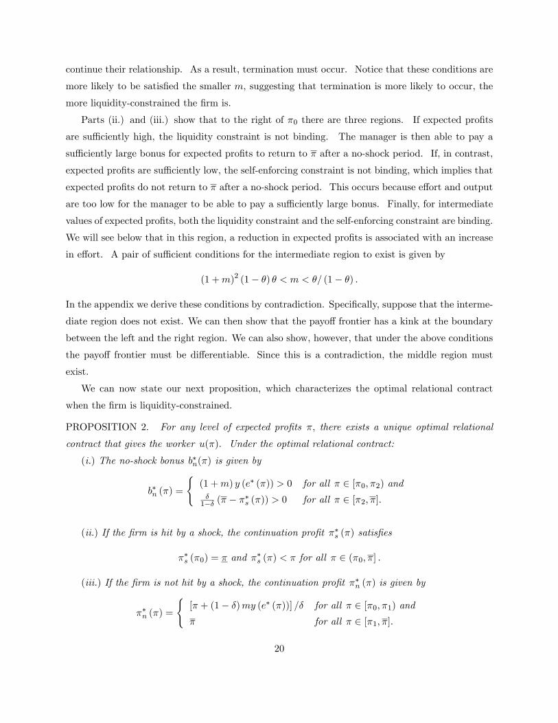
Parts (ii.) and (iii.) show that to the right of �0 there are three regions. If expected pro�ts

are su¢ ciently high, the liquidity constraint is not binding. The manager is then able to pay a

su¢ ciently large bonus for expected pro�ts to return to � after a no-shock period. If, in contrast,

expected pro�ts are su¢ ciently low, the self-enforcing constraint is not binding, which implies that

expected pro�ts do not return to � after a no-shock period. This occurs because e¤ort and output

are too low for the manager to be able to pay a su¢ ciently large bonus. Finally, for intermediate

values of expected pro�ts, both the liquidity constraint and the self-enforcing constraint are binding.

We will see below that in this region, a reduction in expected pro�ts is associated with an increase

in e¤ort. A pair of su¢ cient conditions for the intermediate region to exist is given by

(1 +m)2 (1� �) � < m < �= (1� �) .

In the appendix we derive these conditions by contradiction. Speci�cally, suppose that the interme-

diate region does not exist. We can then show that the payo¤ frontier has a kink at the boundary

between the left and the right region. We can also show, however, that under the above conditions

the payo¤ frontier must be di¤erentiable. Since this is a contradiction, the middle region must

exist.

We can now state our next proposition, which characterizes the optimal relational contract

when the �rm is liquidity-constrained.

PROPOSITION 2. For any level of expected pro�ts �, there exists a unique optimal relational

contract that gives the worker u(�). Under the optimal relational contract:

(i.) The no-shock bonus b�n(�) is given by

b�n (�) =

((1 +m) y (e� (�)) > 0 for all � 2 [�0; �2) and�1�� (� � �

�s (�)) > 0 for all � 2 [�2; �].

(ii.) If the �rm is hit by a shock, the continuation pro�t ��s (�) satis�es

��s (�0) = � and ��s (�) < � for all � 2 (�0; �] .

(iii.) If the �rm is not hit by a shock, the continuation pro�t ��n (�) is given by

��n (�) =

([� + (1� �)my (e� (�))] =� for all � 2 [�0; �1) and� for all � 2 [�1; �].

20

(iv.) E¤ort is given by the unique e¤ort level e� (�) that solves

c0 (e)

y0 (e)=

(�u0+ (�) + (1 +m) (1� �)

�1 + u0+ (�

�n (�))

�for all � 2 [�0; �1),

�u0 (�) for all � 2 [�2; �],

and

y (e) = (�� ) = ((1� �)m) for all � 2 [�1; �2) ,

where u0+ (�) denotes the right derivative.

The proposition shows that most of the features of the optimal relational contract are not

a¤ected by liquidity constraints. In particular, part (i.) shows that the manager still motivates

the worker by promising him a strictly positive bonus. Notice, however, that when the liquidity

constraint is binding, that is, � 2 [�0; �2), there is a limit to the size of the bonus. In this region, themanager would like to pay a larger bonus but is constrained to paying b�n (�) = (1 +m) y (e

� (�)).

Part (ii.) shows that, as in the case without liquidity constraints, the worker punishes the

manager for not paying bonuses by gradually reducing expected pro�ts. While downturns are still

gradual, however, part (iii.) shows that recoveries may no longer be instantaneous. Speci�cally,

when � 2 [�0; �1), ��n (�) is strictly less than �, even though the manager is paying the largestpossible bonus. When � 2 [�1; �2) this bonus is su¢ cient to compensate the worker for lettingexpected pro�ts return to �. When � 2 [�0; �1), however, the largest possible bonus is too smallto compensate the worker. The manager then needs to spread the bonus payments over multiple

periods. Liquidity constraints therefore slow down recoveries from su¢ ciently severe downturns.

Together with the Lemma 6, part (ii.) also implies that the relationship terminates if �0 > �

and the �rm is hit by shocks in su¢ ciently many consecutive periods. The reason is that after a

su¢ ciently severe downturn the manager�s reward for paying a bonus is limited since it then takes

multiple periods for expected pro�ts to return to their upper bound. To ensure that the manager

stays truthful, the worker therefore has to increase the punishment for the manager not paying the

bonus. Since expected pro�ts are already small, the only way to do so is to increase the threat of

termination.

Finally, part (iv.) shows how liquidity constraints a¤ect e¤ort provision. When the liquidity

constraint is not binding, that is, � 2 [�2; �], the expression that determines e¤ort is the same as inthe model without liquidity constraints. In particular, the ratio of marginal e¤ort costs to marginal

output is again equal to the negative of the slope of the payo¤ frontier. In contrast, when the

liquidity constraint is binding, that is, � 2 [�0; �2), the ratio of marginal e¤ort costs to marginaloutput is always strictly larger than the negative of the slope of the payo¤ frontier. The reason

21

is that an increase in e¤ort now has the additional bene�t of relaxing the liquidity constraint. If

� 2 [�0; �1), this additional bene�t is captured by the second term on the right hand side of the

expression in part (iv.). And if � 2 [�1; �2), e¤ort is raised just enough for expected pro�ts toreturn to � following a no-shock period. Notice that in this region e¤ort is decreasing in expected

pro�ts. The worker, therefore, responds to a reduction in expected pro�ts by providing more e¤ort

rather than less. Essentially, the worker understands that providing more e¤ort relaxes the �rm�s

liquidity constraint which, in turn, allows the manager to pay him a larger bonus if the �rm is not

hit by another shock. As discussed in the Introduction, this reasoning is broadly consistent with

the experience at Lincoln Electric.

In summary, liquidity constraints limit the manager�s ability to manage con�icts, which slows

down recoveries and can lead to termination. Liquidity constraints, however, can also induce the

worker to respond to a con�ict by providing more e¤ort rather than less.

7 Discussion

In this section we revisit key features and assumptions of our model and examine them in more

detail. We focus on our main model without liquidity constraints.

7.1 The Failure to Achieve First-Best

We show in Appendix C (Proposition C1) that the Folk Theorem holds in our setting. Speci�cally,

we show that as the discount factor � goes to one, the limit set of the PPE payo¤ contains the

interior of the set of feasible payo¤s. Joint surplus therefore converges towards �rst-best as the

parties become increasingly patient. It is important to note, however, that as long as the discount

factor � is strictly less than one, joint surplus is strictly less than �rst-best. For any � < 1 the

optimal relational contract is therefore ine¢ cient. This is in line with related repeated games such

as Hertel (2004) in which �rst-best also cannot be achieved. In contrast, �rst-best can be achieved,

for instance, in Athey and Bagwell (2001).

The reason for the parties�inability to achieve �rst-best is that the worker can never be sure

that opportunity costs are low. The fact that the worker can never be sure that opportunity costs

are high, in contrast, does not matter for the parties�inability to achieve �rst-best. To see this,

suppose that whenever the �rm is not hit by a shock, there is some probability p 2 [0; 1) withwhich it becomes publicly known that the �rm�s opportunity costs are low. And whenever the

�rm is hit by a shock, there is some probability q 2 [0; 1) with which it becomes publicly knownthat the �rm�s opportunity costs are high. If p = q = 0, this model is the same as our main model.

22

And if either p or q were equal to one, the state would be publicly observed and there would be no

need for the manager to be punished on the equilibrium path. We discuss this public information

benchmark in the next section. In Appendix C (Proposition C2) we show that in the setting in

which p 2 [0; 1) and q 2 [0; 1), �rst-best can be achieved for su¢ ciently high discount factors if andonly if p > 0. Essentially, when p > 0, the manager does not pay the worker when the �rm is hit

by a shock but promises him a larger bonus in the next period in which it is publicly observed that

the �rm�s opportunity costs are low. Since the occurrence of such an event is publicly observable,

the manager�s promise is credible and �rst-best is feasible.

Firms that ask their workers to accept cuts to their compensation often open their books to

prove that those cuts really are necessary (see, for instance, the Introduction and Englmaier and

Segal (2011)). The above argument suggests that �rms should not only open their books during

hard times, in the hope of avoiding worker punishments. Instead, it may be even more important

for �rms to keep their books open during good times, so as to make punishments less costly.

7.2 Benchmarks: Public Information and Long-Term Contracts

The �rst benchmark we examine is one in which shocks are publicly observed. In Appendix C

(Proposition C3) we examine this case and characterize the PPE payo¤ set. For every payo¤ pair

on the PPE frontier we then characterize the optimal relational contract supporting it. As in

our main model, expected pro�ts, e¤ort, and joint surplus jump to their upper bounds following

a no-shock period. Because of the public observability of the opportunity costs, however, shocks

no longer lead to a reduction in expected pro�ts. Instead, following a shock period, expected

pro�ts, e¤ort, and joint surplus remain unchanged. They therefore reach their highest achievable

levels with probability one and then stay there forever. Finally, if the manager and the worker

are patient enough, those highest achievable levels are equal to �rst-best. The evolution of the

relationship between the manager and the worker therefore depends crucially on whether shocks

are publicly observed.

The second benchmark we examine is one in which the manager can commit to a long-term

contract. Suppose that in any period t the manager �rst observes the state �t 2 fn; sg and thenmakes an announcement mt 2 fn; sg about the state. Suppose also that before the �rst period, themanager can commit to a contract that, for any period t, maps her announcements (m1;m2,...;mt)

into the bonus bt that she has to pay the worker at the end of period t.

A long-term contract does not allow the parties to achieve �rst-best. It does, however, allow

them to approximate �rst-best. To see this, let �(t) denote the number of consecutive periods

23

immediately preceding t in which the manager did not pay the worker. Now consider a contract

with three features. First, the contract asks the worker to provide �rst-best e¤ort in all periods.

If the worker ever does not provide �rst-best e¤ort, the manager will never again pay him. Second,

the contract speci�es that if, in period t, the manager announces that the �rm has not been hit by

a shock, she pays the worker a bonus

bt (�(t)) =

�1 +

1

�+1

�2+ :::+

1

��(t)

��u+ c

�eFB

��:

And third, the contract speci�es the maximum number of consecutive periods T � 1 that the

manager can go without paying the worker the bonus. In particular, if, in period t, the manager

announces that the �rm has been hit by a shock and if �(t) < T , the manager does not have to

pay the worker. If, however, �(t) = T , the manager has to pay the worker a bonus bt (T ).

In Appendix C (Proposition C4) we show that under such a contract, the worker always pro-

vides �rst-best e¤ort and the manager always announces the state truthfully. Essentially, under

this contract the manager has to pay the worker�u+ c

�eFB

��per period, independent of her an-

nouncements. By lying about the state, the manager can therefore a¤ect the timing of payments

but not their net present value.

This contract does not achieve �rst-best since it induces ine¢ cient payment whenever the �rm

is hit by shocks in T consecutive periods. By agreeing to a large T , however, the parties can come

arbitrarily close to achieving �rst-best. The evolution of the relationship between the manager and

the worker therefore depends crucially on whether the manager is able to commit to a long-term

contract. And as we saw above, it also depends on whether shocks are privately observed.

8 Conclusions

In a well-known article in The New Yorker, Stewart (1993) describes the upheavals at the investment

bank Credit Suisse First Boston (CSFB) after consecutive years of disappointing bonus payments.

Problems started in 1991 when traders demanded that management pay them a higher bonus.

Management, however, stood �rm, insisting that a higher bonus was not justi�ed because of the

need to �build capital.� To appease the traders, management then simply �promised that 1992 would

be di¤erent� that salaries and bonuses would again be competitive.� Traders were forthcoming in

expressing their disappointment but their retaliations were limited. The traders�behavior changed

the following year, however, when bonus payments were once again below expectations. This time

�many traders seemed to drag their heels, further depressing the �rm�s earnings�and �defections [...]

increased as soon as First Boston actually began paying bonuses.� This response forced management

24

to adapt its compensation policy by formally committing to �guaranteed pay raises,�in some cases

as much as 100%.

At the heart of the con�ict at CSFB was uncertainty, and possibly private information, about

the opportunity costs of bonus payments. In particular, while there was no disagreement about the

traders�performance, there was disagreement about the extent to which bonus payments should be

contingent on the need to �build capital.� The aim of this paper was to explore the con�icts that

arise in such a setting. In our model, it is optimal for the manager to make payments contingent

on their opportunity costs, even though this makes con�icts inevitable. As in the CSFB example,

the manager responds to such con�icts by adapting compensation to their duration, moving from

the informal� promising that 1992 will be di¤erent� to the formal� committing to guaranteed pay

raises. Because the manager responds to a con�ict by changing the compensation she o¤ers the

worker, con�icts evolve gradually. This is again illustrated in the CSFB example in which traders

did not switch from cooperation to punishment abruptly. Instead, the relationship deteriorated

gradually in response to repeated disagreements about bonus pay. Finally, in our main model,

expected pro�ts cycle inde�nitely. The relationship between the manager and the worker therefore

never terminates, nor does it reach a steady state. This is in contrast to the CSFB example where

many traders did leave. Termination, however, can also arise in our setting once we allow for the

�rm to be liquidity-constrained.

To discuss the empirical implications and testability of our model, it is useful to note that the

basic structure of the stage game is closely related to a �trust game.� In a standard trust game,

the �proposer��rst decides on the size of a monetary gift that he makes to the �responder.� The

gift is then increased by some amount after which the responder decides how much to give back to

the proposer. One can therefore view our model as an in�nitely repeated trust game in which the

responder faces shocks to the costs of giving back. There is an extensive literature in experimental

economics that examines trust games. This suggests that one could test our model in a laboratory

setting. Two predictions, in particular, are clear cut. First, the evolution of trust� as measured

by the size of the gift� depends crucially on whether shocks are publicly observed. If shocks are

publicly observed, trust increases over time until it tops out at some level. If shocks are instead

privately observed, trust evolves through booms and busts. Second, the long-term prospects of

a relationship depend on whether the responder is liquidity-constrained. If the responder is not

liquidity-constrained, the relationship continues forever. But if she is liquidity-constrained, it is

certain to terminate eventually.

We have cast our model in the context of an employment relationship. The main ingredients of

25

the model� repeated interaction, limited commitment, and ine¢ cient transfers� are also relevant

in many other economic settings. One example is the lending relationship between an entrepreneur

and an investor who are not able to commit to long-term contracts. The entrepreneur can have

private information about her marginal value of money and the investor can adjust his future

�nancing terms based on the payment history of the entrepreneur. Another example is that of

long-term and informal supplier relationships in which buyers face shocks to their ability to pay

their suppliers. In 1995, for instance, Continental Airlines was close to bankruptcy and its �most

pressing need was to shore up its cash position. The airline [...] was only able to make its January

1995 payroll when [its CEO] Bethune successfully begged Boeing to return cash deposits on aircraft

whose delivery he had deferred� (Frank 2009). A �nal example involves the informal insurance

relationships among farmers in developing countries. There is some evidence that the farmers�

income is private information (see, for example, Kinnan (2011)). While most of the literature has

focused on moral hazard and insurance issues separately, our model suggests that these issues are

related since insurance decisions a¤ect future production choices.

26

9 Appendix A: Main Model

Proof of Lemma 1: Part (i.): Note that � and u are the manager�s and the worker�s minmax

payo¤s and that they can be sustained as PPE payo¤s by having each party take their outside

option in each period. It is then immediate that in any PPE the bonus payments, wages, and

e¤ort are bounded. As a result, we can restrict the manager�s and the worker�s actions to compact

sets. Standard arguments then imply that the PPE payo¤ set E is compact so that

u(�) = maxfu; (�; u) 2 Eg:

Part (ii.): Since there is a public randomization device, any payo¤ on the line segment between

(�; u) and (�; u) can be supported as a PPE payo¤. It then follows that randomization between

(�; u) and (�; u(�)) allows us to obtain any payo¤ (�; u0) for all u0 2 [u; u(�)]:Part (iii.): Suppose to the contrary that u(�) > u: Note that since (�; u(�)) is an ex-

tremal point of E it must be sustained by pure actions in period 1. Consider a PPE with pay-

o¤s (�; u(�)) and associated �rst-period actions (e; w; bs; bn) and �rst-period continuation payo¤s

(�s; �n; us; un). Now consider an alternative strategy pro�le with the same �rst-period continuation

payo¤s (�s; �n; us; un) but in which �rst-period actions are given by (be; bs; bn; w), where be = e+ ".It follows from the promise keeping constraints PKM and PKW that under this alternative strategy

pro�le the payo¤s are given by

b� = � ((1� �) (y (be)� (1 + �)(w + bs)) + ��s) + (1� �) ((1� �) (y (be)� w � bn) + ��n)and bu = �((1� �) (w + bs) + �us) + (1� �) ((1� �) (w + bn) + �un)� (1� �) c (be) .Notice that since y is increasing, we have that b� > �. Moreover, for small enough ", bu � u. It canbe checked that this alternative strategy pro�le satis�es all the constraints in Section 4.1. (with

the exception of the ICW constraint that we ignore throughout) and therefore constitutes a PPE.

Since b� > � this contradicts the de�nition of �. �Proof of Lemma 2: Part (i.): We proceed in two steps. First, we show that, for any �1 < �2,

if both u(�1) and u(�2) can be sustained by pure actions in the stage game other than taking the

outside option, then u(�) can also be sustained by pure actions for any � 2 (�1; �2). Second, we

then show that u(�) is supported by a pure action in the stage game without taking the outside

option. Since we know from the proof of Lemma 1 that u(�) can sustained by pure actions, the

result follows.

27

We prove the �rst step by contradiction. Consider any �1 < �2 such that u(�1) and u(�2)

can be sustained by pure actions in the stage game. Take any � 2 (�1; �2) and suppose to

the contrary that (�; u (�)) is not sustained by pure actions. Then there exists a � 2 (0; 1), ae�1 2 [�1; �), and a e�2 2 (�; �2] such that (i.) (e�1; u (e�1)) and (e�2; u (e�2)) are sustained by pureactions, (ii.) � = �e�1 + (1� �) e�2, and (iii.) u (�) = �u (e�1) + (1� �)u (e�2) : Now consider a

PPE with payo¤s (e�j ; u (e�j)), for j = 1; 2, and associated �rst-period actions (ej ; bsj ; bnj ; wj) and�rst-period continuation payo¤s (�sj ; �nj ; usj ; unj ). De�ne be as the e¤ort level satisfying

y(be) = �y(e1) + (1� �)y(e2):Since y is strictly concave, we have that

y(�e1 + (1� �)e2) > �y(e1) + (1� �)y(e2) = y (be) :And since y is strictly increasing this implies that

be < �e1 + (1� �)e2:Now consider an alternative strategy pro�le with �rst-period actions (be; bw;bbs;bbn) and �rst-period

continuation payo¤s (b�s; b�n; bus; bun), where bw = �w1+ (1� �)w2 and where bbs;bbn; b�s; b�n; bus;and bunare de�ned analogously.

Also, let bw = �w1 + (1� �)w2 and de�ne bbs;bbn; b�s; b�n; bus, and bun analogously. It follows fromthe promise keeping constraints PKM and PKW that under this alternative strategy pro�le the

payo¤s are given by b� = �e�1 + (1� �)e�2 andbu = �u(e�1) + (1� �)u(e�2) + (1� �) (�c(e1) + (1� �) c(e2)� c(e)) :

Since c (e) is strictly increasing and strictly convex, it follows that bu > �u(e�1) + (1 � �)u(e�2). It

can be checked that this alternative pro�le satis�es all the constraints in Section 4.1. and therefore

constitutes a PPE. Since bu > �u(e�1) + (1� �)u(e�2), this proves the �rst step.To prove the second step, suppose to the contrary that u(�) cannot be sustained by pure actions

other than taking the outside options. Since (�; u(�)) is an extremal point, it cannot be sustained

by randomizations. The parties must therefore take their outside options in period 1, which implies

that u(�) = u.

Now choose a payo¤ pair (�; u(�)) that is sustained by pure actions other than the outside

option. Notice that such a payo¤ pair must exist since (�; u(�)) is an extremal point that is

sustained by pure actions. Suppose (�; u(�)) is obtained by a PPE with �rst-period actions

28

(e; w; bs; bn) and �rst-period continuation payo¤s (�s; �n; us; un). Next, consider an alternative

strategy pro�le with the same �rst-period continuation payo¤s (�s; �n; us; un) but di¤erent �rst-

period actions (e; bw; bs; bn); where bw = w + " for some " > 0. This strategy pro�le generates

payo¤s (b�; bu) ; where b� = � � (1� �) (1 + ��) " and bu = u(�) + (1� �) ". It can be checked

that as long as b� � � or, equivalently, " � (� � �) = ((1� �) (1 + ��)), this alternative strategypro�le satis�es all of the constraints in Section 4.1 and therefore constitute a PPE. Let " =

(� � �) = ((1� �) (1 + ��)) : The above then implies that (�; u(�) + (� � �) =(1 + ��)) is a PPEpayo¤, which contradicts u(�) = u:

Finally, notice that by sending " to zero, the above implies that u0�(�) � �1=(1 + ��) for all� > �. Below we will use this fact to prove part (iii.).

Part (ii.): Concavity follows directly from the availability of the public randomization device.

Part (iii.): Consider a PPE with payo¤s (�; u (�)), where � 2 (�; �), and associated �rst-

period actions (e; w; bs; bn) and �rst-period continuation payo¤s (�s; �n; us; un). Now consider an

alternative pro�le with the same �rst-period continuation payo¤s (�s; �n; us; un) but in which �rst-

period actions are given by (be; w; bs; bn), where be = e+ " for some " > 0. It follows from PKM and

PKW that under this strategy pro�le the payo¤s are given by b� = �+(1� �) (y(e+ ")� y(e)) andbu = u(�)�(1� �) (c(e+ ")� c(e)). For small enough ", the alternative strategy pro�le satis�es allthe constraints in Section 4.1. (with the exception of the ICW constraint that we ignore throughout)

and therefore constitutes a PPE.

Since u (�) is the frontier, it must be that

u (� + (1� �) (y(e+ ")� y(e))) � bu = u(�)� (1� �) (c(e+ ")� c(e)):Sending " to zero, we then obtain that

� c0 (e)

y0 (e)� u0+(�):

Since u is concave and, as shown in the proof of part (ii.), u0�(�) < �1=(1 + ��), we haveu0+(�) � u0�(�) < �1=(1 + ��). This implies that

c0 (e)

y0 (e)� 1

1 + ��:

Since c0 (e) =y0 (e) = 0 for e = 0, we therefore have e > 0. Next, consider another alternative

strategy pro�le with �rst-period actions (be; w; bs; bn), where be = e � " for small " > 0, and �rst-

period continuation payo¤s (�s; �n; us; un). Proceeding in exactly the same way, it can be shown

that u0�(�) � �c0 (e) =y0 (e). This implies that u0+(�) = u0�(�) and thus u is di¤erentiable. Since

29

we have u0�(�) � �1=(1 + ��) this concludes the proof except for the claim that �1 < u0(�). Forsimplicity of exposition we will prove this part after Lemma 5. The proofs of Lemmas 3-5 do not

make use of this claim. �

Proof of Lemma 3: Recall from Lemma 1 that the PPE payo¤ set is compact. Consider a PPE

with payo¤s (�; u(�)) and associated �rst-period actions (e; w; bs; bn) and �rst-period continuation

payo¤s (�s; �n; us; un). Suppose to the the contrary of the claim that us < u(�s). Now consider an

alternative strategy pro�le with the same �rst-period actions but in which �rst-period continuation

payo¤s are given by (�s; �n; bus; un) ; where bus = us + " and where " > 0 is small enough such thatus + " � u (�s). It follows from the promise keeping constraints PKM and PKW that under this

alternative strategy pro�le the payo¤s are given by b� = � and bu = u(�) + �(1 � �)" > u(�). It

can be checked that this alternative strategy pro�le satis�es all the constraints in Section 4.1 (with

the exception of the ICW constraint that we ignore throughout) and therefore constitutes a PPE.

Since bu > u(�) this contradicts the de�nition of u(�). Thus it must be that us = u(�s). The

proof for un = u(�n) is analogous. �

Proof of Lemma 4: Part (i.): By combining the truth-telling constraints TTN and TTS we have

(1 + �) (1� �) (bn � bs) � � (�n � �s) � (1� �) (bn � bs):

Since (1 + �) > 0, this implies that bn � bs � 0.Next, consider a PPE with payo¤s (�; u(�)) and associated �rst-period actions (e; w; bs; bn)

and �rst-period continuation payo¤s (�s; �n; us; un) and suppose that bs > 0. Now consider an

alternative strategy pro�le with the same continuation payo¤s (�s; �n; us; un) but in which �rst-

period actions are given by (e; bw;bbs;bbn), where bw = w + bs, bbs = 0, and bbn = bn � bs. It follows

from the promise keeping constraints PKM and PKW that under this alternative strategy pro�le the

payo¤s are given by (�; u(�)). It can be checked that this alternative strategy pro�le satis�es all

the constraints in Section 4.1. (with the exception of the ICW constraint that we ignore throughout)

and therefore constitutes a PPE. This proves part (i.).

Part (ii.): Consider a PPE with payo¤s (�; u(�)) and associated �rst-period actions (e; w; bs; bn)

and �rst-period continuation payo¤s (�s; �n; u (�s) ; u (�n)). Suppose that for this PPE the TTN

is slack, that is, � (�n � �s) > (1� �) (bn � bs). Together with the non-reneging constraint

NRS this implies that NRN is slack. Now consider an alternative strategy pro�le with the

same �rst-period actions (e; w; bs; bn) but in which �rst-period continuation payo¤s are given by

(b�s; b�n; u (b�s) ; u (b�n)), where b�s = �s + (1� �)" and b�n = �n � �" for " > 0. It follows from the

promise keeping constraints PKM and PKW that under this strategy pro�le the payo¤s are given

30

by b� = � andbu = (1� �) (w + �bs + (1� �) bn � c (e)) + �(�u (b�s) + (1� �)u (b�n)).

From the concavity of u it then follows that

bu � (1� �) (w + �bs + (1� �) bn � c (e)) + �(�u (�s) + (1� �)u (�n)) = u (�) :It can be checked that for su¢ ciently small " this alternative strategy pro�le satis�es all the

constraints in Section 4.1. (with the exception of the ICW constraint that we ignore throughout)

and therefore constitutes a PPE. Since bu � u (�) this implies that for any PPE with payo¤s

(�; u(�)) for which TTN is not binding there exists another PPE for which TTN is binding and

which gives the parties weakly larger payo¤s. �

Proof of Lemma 5: By Lemma 2, every point on the PPE frontier can be supported by pure

actions other than the outside options. Lemma 3 and the de�nition of u then imply that �+ u(�)

is given by

� + u(�) = maxe;w;�s;�n

(1� �) (y (e)� c (e)) + �� (�s + u (�s)) + (1� �) � (�n + u (�n))� (1� �) ��w

subject to the constraints in Section 4.1. (with the exception of the ICW constraint that we ignore

throughout). Notice that we have used Lemma 4 to substitute out bs and bn in the objective

function.

To reduce the number of constraints, consider �rst the feasibility constraints. By Lemma 4

the non-negative constraints NNS is no longer relevant. At the end of this proof we show that the

non-negativity constraint NNN is also no longer relevant. Moreover, in the proof of Lemma 2 we

showed that c0 (e) =y0 (e) � 1= (1 + ��) : We therefore have e (�) > 0 for all � 2 [�; �] which impliesthat NNe is slack.

Next, Lemma 3 implies that SEN and SES can be reduced to � � �s � � and � � �n � �. Theonly relevant feasibility constraints are therefore given by NNW , SEN, and SES.

Next, we examine the no deviation constraints with the exception of the ICW constraint which

we ignore throughout. Part (i.) of Lemma 4 and SES imply that NRN and NRS are satis�ed. Part

(ii.) of Lemma 4 further implies that TTN and TTS are satis�ed.

Next, we turn to the promise-keeping constraints. We obtain the version of the PKM constraint

in the lemma by using Lemma 4 to substitute bs and bn out of the original PKM constraint. The

PKW constraint is satis�ed because �+u(�) is the solution to the functional equation given by the

constrained maximization problem.

31

Finally, consider the non-negativity constraint NNN. Notice �rst that NNN is equivalent to

�s � �n. Now consider a PPE with payo¤s (�; u(�)) and associated �rst-period actions (e; w) and�rst-period continuation payo¤s (�s; �n). Suppose to the contrary of the claim that �n < �s. There

then exists an alternative strategy pro�le that satis�es all the constraints in Lemma 5 and generates

a strictly larger joint surplus, leading to a contradiction. Speci�cally, consider an alternative

strategy pro�le with the same �rst-period actions (e; w) but in which the �rst-period continuation

payo¤s are given by (�s; b�n), where b�n = �n+ " for some " > 0. Since, by Lemma 2, 1+u0(�) > 0for all � 2 [�; �], the alternative strategy pro�le generates a strictly larger joint surplus � + u(�).Moreover, it can be checked that this alternative strategy pro�le satis�es all the constraints in

Lemma 5. As claimed above, the non-negativity constraint NNN is therefore no longer relevant.

�Proof of the last part of Lemma 2 (�1 < u0(�)): The Lagrangian associated with the

maximization problem in Lemma 5 is given by

� + u (�) = L = (1� �) (y (e)� c (e)) + �� (�s + u (�s)) + (1� �) � (�n + u (�n))� (1� �) ��w

+�1(� � (1� �) y (e)� ��s + (1� �) (1 + ��)w)

+�2(��s � ��) + �3(1� �)w + �4(�� n);

where we use the fact that �s � �n (as shown in the proof of Lemma 5) to eliminate the constraints�s � � and �n � �. Note that this is a well-de�ned concave program. The �rst order conditionswith respect to �n, �s, w, and e are given by

(1� �)(1 + u0 (�n))� �4 = 0; (FOCN)

�(1 + u0 (�s))� �1 + �2 = 0; (FOCS)

��+ �1 (1 + ��) + �3 = 0; (FOCW)

and

y0 (e)� c0 (e)� �1y0(e) = 0: (FOCe)

Furthermore, the envelope condition is given by

1 + u0(�) = �1: (envelope)

To prove that u0(�) > �1 for all � 2 [�; �], note that FOCS and FOCN imply that

�1 = �(1 + u0 (�s)) + �2

� �(1 + u0 (�n))

� 0:

32

It therefore follows from the envelope condition that 1 + u0(�) � 0 for � 2 [�; �].To �nish the proof, we need to rule out that u0(�) = �1 for all � 2 [�; �]. Suppose the contrary

and de�ne � � f� 2 [�; �] ju0(�) = �1g. We now establish three facts. First, if � 2 � then�s(�) 2 �. This follows from FOCS, �1 = 0, and �2 � 0. Second, if � 2 � then e(�) = eFB, whereeFB is the �rst-best e¤ort level that solves y0 (e) = c0 (e). This follows from FOCe and �1 = 0.

Finally, if � 2 � then w(�) = 0. To see this, note that since �1 = 0, FOCW implies that �3 > 0.

It then follows from the complementarity slackness condition with respect to NNW that w(�) = 0.

The three facts above imply that the manager can maximize her pay by always claiming to have

been hit by a shock. This is a contradiction since the (�c(eFB)) would then be smaller than hisoutside option. �

Proof of Proposition 1: We �rst continue to ignore the ICW constraint. For this relaxed

problem we �rst prove parts (i.) to (v.) and then show that the optimal relational contract is

unique. Finally, we show that the optimal relational contract of the relaxed problem satis�es the

ICW constraint.

Parts (i.) to (v.): The expression for bn in part (i.) follows from the TTN constraint. The fact

that bn > 0 follows from ��s < � which is shown in part (ii.).

For part (ii.) consider FOCS. Suppose �rst that �2 > 0. In this case, the complementarity

condition associated with SES implies that �s = �. Suppose next that �2 = 0. In this case

1 + u0 (�s) =1

��1 =

1

�(1 + u0 (�));

where the �rst equality follows from FOCS and the second equality follows from the envelope

condition. Since Lemma 2 implies that 1 + u0 (�) > 0, we have that u0 (�s) > u0 (�). Part (ii.)

then follows from the concavity of u.

Part (iii.) follows from 1 + u0 (�) > 0 and FOCN.

Part (iv.) follows from combining FOCe and the envelope condition. Note that since c0 (e) =y0 (e)

is strictly increasing, e�(�) is unique.

For part (v.), recall from Lemma 2 that u0(�) � �1= (1 + ��). Suppose �rst that u0(�) <

�1= (1 + ��) for all � 2 [�; �] : In this case, FOCW and the envelope condition imply that w � 0.Suppose next that there exists a line segment with u0(�) = �1= (1 + ��). Recall that be is theunique e¤ort level satisfying c0(be)=y0(be) = 1= (1 + ��). Part (iv.) implies that on the line segment

33

e = be. Moreover, we must have �s = �. To see this, note that FOCS implies that�2 = �1 � �(1 + u0 (�s))

=��

1 + �� (1 + u0 (�s))

� (1� �) ��

1 + ��;

where the inequality follows from u0 (�s) � �1=(1+��). Since �2 > 0, the complementary slacknesswith respect to SES then implies that �s = �: Since �s(�) = � and e(�) = be for � on the linesegment, the PKM constraint implies that w�(�) = ((1� �)y(be) + �� )= ((1� �)(1 + ��)). Thisproves part (v.).

Uniqueness: Note that in all of the derivations above, e�(�); w�(�); and ��n(�) are unique.

Moreover, PKM implies that ��s(�) is unique. This proves that the optimal relational contract is

unique as long as TTN is binding. In Lemma 4 we showed that for any optimal relational contract

there exists an equivalent one in which TTN is binding. Next we show that TTN has to be binding

for all optimal relational contracts.

For this purpose, suppose to the contrary that there exists an optimal relational contract for

which TTN is not binding. This implies that there exists a PPE with payo¤s (�; u(�)) and asso-

ciated �rst-period actions (e; w; bs; bn) and �rst-period continuation payo¤s (�s; �n; u (�s) ; u (�n))

such that

� (�n � �s) > (1� �) (bn � bs) .

Now consider an alternative strategy pro�le with the same �rst-period actions (e; w; bs; bn) but in

which �rst-period continuation payo¤s are given by (b�s; b�n; u (b�s) ; u (b�n)), where b�s = �s+(1��)"and b�n = �n � �": It can be checked that when " = [� (�n � �s)� (1� �) (bn � bs)] =�, thisalternative strategy pro�le satis�es all the constraints in Section 4.1. and is therefore constitutes a

PPE with payo¤s (�; u(�)) : Moreover, the TTN constraint is binding since

� (b�n � b�s) = � (�n � �s)� �" = (1� �) (bn � bs) :Notice that under this alternative strategy pro�le b�n < �. This is a contradiction since we saw

above that when TTN is binding, the optimal relational contract must have ��n (�) = �.

Checking that ICW is satis�ed: Recall that the ICW constraint is given by �u+(1� �)w�(�) �u(�): The constraint is clearly satis�ed when w = 0, that is, for all � � b�:

For � < b�; part (v.) implies thatd(�u+ (1� �)w�(�))

d�= � 1

1 + ��= u0(�);

34

which in turn implies that

u(�)� (�u+ (1� �)w�(�))

= u(b�)� (�u+ (1� �)w�(b�))> 0:

This shows that ICW is satis�ed for all � 2 [�; �]: �

35

References

[1] Abdulkadiroglu, Atila and Kyle Bagwell. 2010. Trust, Reciprocity and Favors in

Cooperative Relationships. Mimeo.

[2] Abreu, Dilip, David Pearce, and Ennio Stacchetti. 1990. Toward a Theory of Dis-

counted Repeated Games with Imperfect Monitoring, Econometrica, 58(5): 1041-1063.

[3] Athey, Susan and Kyle Bagwell. 2001. Optimal Collusion with Private Information,

The RAND Journal of Economics, 32 (3): 428-465.

[4] � � � �and � � � �. 2008. Collusion with Persistent Cost Shocks, Econometrica, 76(3):

493-540.

[5] � � � �, � � � �, and Chris Sanchirico. 2004. Collusion and Price Rigidity, Review of

Economic Studies, 71 (2): 317-349.

[6] Biais, Bruno, Thomas Mariotti, Guillaume Plantin, and Jean-Charles Rochet.

2007. Dynamic Security Design: Convergence to Continuous Time and Asset Pricing Impli-

cations, Review of Economic Studies, 74(2): 345-390.

[7] Baker, George, Robert Gibbons, and Kevin Murphy. 1994. Subjective Performance

Measures in Optimal Incentive Contract, Quarterly Journal of Economics, 109(4): 1125-1156.

[8] � � � �, � � � �, and � � � �. 2002. Relational Contracts and the Theory of the Firm,

Quarterly Journal of Economics, 117(1): 39-84.

[9] Clementi, Gian Luca and Hugo Hopenhayn. 2006. A Theory of Financing Constraints

and Firm Dynamics, Quarterly Journal of Economics, 121(1): 229-265.

[10] Chassang, Sylvain. 2010. Building Routines: Learning, Cooperation, and the Dynamics of

Incomplete Relational Contracts, American Economic Review, 100(1): 448-465.

[11] Che, Yeon-Koo and Seung-Weon Yoo. 2001. Optimal Incentives for Teams. American

Economic Review, 91(3): 525-541.

[12] DeMarzo, Peter and Yuliy Sannikov. 2006. Optimal Security Design and Dynamic

Capital Structure in a Continuous-Time Agency Model, Journal of Finance, 61: 2681-2724.

[13] � � � � and Michael Fishman. 2007. Optimal Long-Term Financial Contracting with

Privately Observed Cash Flows, Review of Financial Studies, 20(6): 2079-2128.

36

[14] Englmaier, Florian and Carmit Segal. 2011. Cooperation and Con�ict in Organiza-

tions. Mimeo.

[15] Fong, Yuk-fai and Jin Li. 2010. Relational Contracts, E¢ ciency Wages, and Employment

Dynamics. Mimeo.

[16] Frank, Douglas. 2009. Continental Airlines: The Go Forward Plan, INSEAD Case, No.

10/2009-5565.

[17] Fuchs, William. 2007. Contracting with Repeated Moral Hazard and Private Evaluations,

American Economic Review, 97(4): 1432-1448.

[18] Green, Edward and Robert Porter. 1984. Noncooperative Collusion under Imperfect

Price Information, Econometrica, 52(1): 87-100.

[19] Halac, Marina. Forthcoming. Relational Contracts and the Value of Relationships, Amer-

ican Economic Review.

[20] Hastings, Donald. 1999. Lincoln Electric�s Harsh Lessons from International Expansion,

Harvard Business Review, 77(3): 162-178.

[21] Hauser, Christine and Hugo Hopenhayn. 2008. Trading Favors: Optimal Exchange

and Forgiveness. Mimeo.

[22] Hertel, Johanna. 2004. E¢ cient and Sustainable Risk Sharing with Adverse Selection.

Mimeo.

[23] Kinnan, Cynthia. 2011. Distinguishing Barriers to Insurance in Thai Villages. Mimeo.

[24] Kocherlakota, Narayana. 1996. Implications of E¢ cient Risk Sharing without Commit-

ment, Review of Economic Studies, 63(4): 595-610.

[25] Levin, Jonathan. 2002. Multilateral Contracting and the Employment Relationship, Quar-

terly Journal of Economics, 117(3): 1075-1103.

[26] � � � �. 2003. Relational Incentive Contracts, American Economic Review, 93 (3): 835-857.

[27] Ligon, Ethan, Jonathan Thomas, and Tim Worrall. 2002. Informal Insurance

Arrangements in Village Economies, Review of Economic Studies, 69(1): 209-244.

37

[28] MacLeod, Bentley. 2007. Reputations, Relationships and Contract Enforcement, Journal

of Economic Literature, 45(3): 597-630.

[29] � � � �and James Malcomson. 1989. Implicit Contracts, Incentive Compatibility, and

Involuntary Unemployment, Econometrica, 57 (2): 447-480.

[30] � � � �and � � � �. 1998. Motivation and Markets, American Economic Review, 88(3):

388-411.

[31] Mailath, George and Larry Samuelson. 2006. Repeated Games and Reputations, Ox-

ford University Press.

[32] Malcomson, James. Forthcoming. Relational Incentive Contracts, to be published in the

Handbook of Organizational Economics, eds. Robert Gibbons and John Roberts, Princeton

University Press.

[33] Mobius, Markus. 2001. Trading Favors. Mimeo.

[34] Mukherjee, Arijit and Luis Vasconcelos. 2011. Optimal Job Design in the Presence

of Implicit Contracts, The RAND Journal of Economics, 42(1): 44-69.

[35] Padro i Miquel, Gerard and Pierre Yared. 2011. The Political Economy of Indirect

Control. Mimeo.

[36] Rayo, Luis. 2007. Relational Incentives and Moral Hazard in Teams, Review of Economic

Studies, 74(3): 937-963.

[37] Samuelson, Larry. 2006. The Economics of Relationships, Econometric Society Mono-

graphs, 41: 136-185.

[38] Spear, Stephen and Sanjay Srivastava. 1987. On Repeated Moral Hazard with Dis-

counting, Review of Economic Studies, 54(4): 599-617.

[39] Stewart, James. 1993. Taking the Dare, The New Yorker, July 26, 1993: 34-39.

[40] Thomas, Jonathan and Tim Worrall. 1990. Income Fluctuation and Asymmetric Infor-

mation: An Example of a Repeated Principal-Agent Problem, Journal of Economic Theory,

51(2): 367-390.

[41] � � � �and � � � �. 2010. Dynamic Relational Contracts under Limited Liability. Mimeo.

38

[42] Watson, Joel. 1999. Starting Small and Renegotiation, Journal of Economic Theory,

85(1): 52-90.

[43] � � � �. 2002. Starting Small and Commitment, Games and Economic Behavior, 38(1):

176-199.

[44] Yang, Huanxing. 2011. Nonstationary Relational Contracts. Mimeo.

[45] Yared, Pierre. 2010. A Dynamic Theory of War and Peace, Journal of Economic Theory,

145(5): 1921-1950.

39

10 Appendix B (For Online Publication): The E¤ects of LiquidityConstraints

In this appendix we prove the results in Section 6 that analyzes the model with liquidity constraints.

Speci�cally, the �rm is subject to the liquidity constraint that

maxfw + bs; w + bng � (1 +m)y

for some m > 0: This constraint signi�cantly complicates the analysis. In particular, the PPE

frontier is no longer di¤erentiable. To make the analysis more tractable, we assume that the

manager cannot pay the worker in a shock state (� = 1): Consequently, this implies that w � 0and bs � 0:

Since the analysis with the liquidity constraints follows similar steps as the main model, we

omit the proofs for results that are obtained from identical arguments. Below, we �rst describe the

basic properties of the PPE frontier in the background subsection and then prove the main results

in the dynamics subsection. The last subsection provides several su¢ cient conditions that allow

for further characterization of the dynamics.

10.1 Background

Proceeding in the same way as the main model, we can show that when the PPE frontier is

sustainable by pure actions (other than the outside options), the joint surplus � + u (�) is de�ned

recursively by the following problem:

� + u (�) = maxe;�s;�n

(1� �) (y (e)� c (e)) + �� (�s + u (�s)) + (1� �) � (�n + u (�n)) (3)

such that

��n � � + (1� �)my (e) ; (LIQF)

� � �n � �; (LSEN)

� � �s � �; (LSES)

and

� = (1� �) y (e) + ��s: (LPKM)

The problem above corresponds with that in Lemma 5 with several modi�cations. In particular,

LIQF is the extra liquidity constraint for the �rm. In addition, w � 0 implies that NNW is no

40

longer needed. Moreover, w does not appear in the LPKM , and relatedly, the truth-telling condition

under the no-shock state is given by

� (�n � �s) = (1� �) bn: (LTTN)

In addition to these modi�cations, there are several other di¤erences between the main model

and the model with liquidity constraint. First, unlike the main model, it is no longer true that

each point on the PPE frontier can be sustained by pure actions.

LEMMA B1. There exists a critical level of expected pro�ts �0 2 [�; �) such that for all � � �0the PPE frontier u(�) is supported by pure actions and for all � 2 (�; �0) it is supported by

randomization. Speci�cally, for any � < �0 the manager and the worker randomize between

terminating their relationship and playing the strategies that deliver expected payo¤s �0 and u(�0).

Proof: De�ne �0 as the smallest payo¤ of the manager at which u(�0) can be sustained by

pure actions other than the outside options. To see that �0 is well de�ned, let � = f� 2 [�; �]j(�; u(�)) can be supported by pure actions other than the outside optionsg. We need to show

that the set � is non-empty and closed. Note that � 2 � because (�; u(�)), being an extremal

point of the PPE payo¤ set, can be sustained by pure actions, and since � 6= �, the pure actionsthat support (�; u(�)) is not the outside options. To see that � is closed, consider a convergent

sequence f�jg1j=1 � � such that lim�j = �. Let (ej ; bnj ; �sj ; �nj ; usj ; unj ) be the �rst-period

actions and �rst-period continuation payo¤s associated with (�j ; u (�j)). Since the actions and

continuation payo¤s maximize the PPE payo¤, the Maximum Theorem implies that the actions

and continuation payo¤s are upper hemi-continuous in expected pro�ts. We therefore have lim ej =

e(�), lim�sj = �s(�), lim�nj = �n(�), lim bnj = bn(�), limunj = un(�), and limusj = us(�). It

can be checked that the pro�le (e(�); bn(�); �s(�); �n(�); us(�); un(�)) satis�es all the constraints

and supports (�; u(�)), which implies that � 2 �. This shows that �0 is well de�ned.Repeating the proof in Lemma 2, it is immediate that � is convex and thus � = [�0; �]. The

part that for all � � �0 the PPE frontier u(�) is supported by pure actions follows from the

de�nition of �0 and the convexity of �. It remains to show that for any � 2 (�; �0) the managerand the worker randomize between terminating their relationship and playing the strategies that

deliver expected payo¤s �0 and u(�0): Note that if �0 = �; the randomization region does not exist

and there is nothing to prove. Therefore, let us assume that �0 > �: Notice that (�; u(�)) is an

extremal point of the PPE payo¤ set, and since �0 > �; (�; u(�)) must be supported by the outside

options, and therefore, (�; u(�)) = (�; u).

Now for any � 2 (�; �0); (�; u(�)) is sustained by randomization by the de�nition of �0. Since

41

the PPE payo¤ set is two-dimensional and convex and (�; u(�)) is at its boundary, (�; u(�)) can be

expressed as the linear combination of two extremal points. Denote these two points by (�0; u(�0))

and (�00; u(�00)), where �0 < � < �00. Since these are both extremal points they are sustained by

pure actions. Moreover, since �0 < � < �0 and u(�0) is supported by pure actions, we must have

�0 = � by the de�nition of �0: Now by the concavity of u; it is clear that we can have �00 = �0: We

provide the argument that �00 must equal to �0 following Lemma B2, whose proof does not depend

on the uniqueness of �00: �

Second, the PPE frontier u is no longer di¤erentiable for all � for some parameter value m.

However, since u is again concave (given the public randomization device), both the left and the

right derivatives exist. This implies that the results written as equalities of derivatives can be

replaced with a pair of corresponding inequalities involving left and right derivatives.

Third, while it remains true that u0�(�) > �1 for all �; we no longer always have �n = �:

When LIQF binds, �n < �: The lemma below gives the exact expression for �n and proves that

u0�(�) > �1 for all �.

LEMMA B2. u0�(�) > �1; and the continuation payo¤ following a no-shock period is given by thefollowing:

��n (�) = minf�;1

�(� + (1� �)my)g:

Proof: The Lagrangian of the joint surplus associated with the recursive problem is given by

L = (1� �) (y (e)� c (e)) + �� (�s + u (�s)) + (1� �) � (�n + u (�n))

+�1[� � (1� �) y (e)� ��s]

+�2(��s � ��) + �3[� + (1� �)my (e)� ��n] + �4(�� n):

The �rst-order conditions with respect to �s; �n and e are given by

�(1 + u0� (�s)) � �1 � �2 � �(1 + u0+ (�s)) (4)

(1� �)(1 + u0� (�n)) � �3 + �4 � (1� �)(1 + u0+ (�n)) (5)

(1� �1 +m�3)y0 (e)� c0 (e) = 0: (6)

The envelope condition is given by

1 + u0�(�) � �1 + �3 � 1 + u0+(�): (7)

42

Notice that if u0�(�) > �1 for all � 2 [�0; �), the expression for ��n(�) immediately follows. Tosee this, suppose to the contrary that for some �,

��n(�) < minf�;1

�[� + (1� �)my(e(�))]g:

On the one hand, this implies that �4(�) = �3(�) = 0 since the associated constraints are not

binding. As a result, u0+ (�n) � �1 by equation (5). On the other hand, consider �n = �n+ " for" > 0. Since �n < �, we can make " small enough so that �n < �. By the concavity of u, we have

u0+ (�n) � u0� (�n) > �1;

where the second inequality comes from the fact that u0�(�) > �1 for all � 2 [�0; �). This is a

contradiction because we have shown that u0+ (�n) � �1:Now we prove that u0�(�) > �1 for all � 2 [�0; �) in two steps. In step 1, we show that

u0�(�) � �1 for all � 2 [�0; �). Suppose to the contrary that u0�(�) < �1 for some � 2 [�0; �).Then there is a PPE with payo¤ (�; u(�)) such that its �rst-period actions are denoted by (e; bn)

and its �rst-period continuation payo¤s are denoted by (�s; �n; us; un). Notice that �3(�) has to

be zero because otherwise we have

�n =1

�[� + (1� �)my (e)] > �:

Since u0�(�n) � �1 by equation (5), this implies that u0�(�) � u0�(�n) � �1, contradicting theclaim that u0�(�) < �1.

Next, since �2 (�) � 0; (4) and (7) imply that

1 + u0�(�) � �1 � �(1 + u0+ (�s)):

Since u0�(�) < �1, the above inequality means that u0+ (�s) < �1: Notice that if �s < �n, the

concavity of u implies that u0+ (�s) � u0� (�n) � �1, which contradicts u0+ (�s) < �1:As a result, we must have �s = �n. LTTN then implies that bn = 0, and the worker�s promise-

keeping condition then gives that

u(�) = �u(�s)� (1� �)c(e):

This implies u(�s) > u(�); and consequently, �s < � given u is concave and u0�(�) < �1:Now consider an alternative strategy pro�le with �rst-period actions (e; bn) and �rst-period

continuation payo¤s (�s; �n; us; un); where �k = �k + " and uk = u(�k); for k = s; n and " > 0.

43

It can be checked that for small enough ", the alternative strategy pro�le is a PPE with payo¤s

(�; u), where

� = � + �"

u = u(�) + �[u(�s)� u(�s)]:

By the de�nition of u, we have u � u(�). Sending " to zero, we get

u0+(�) � u0+(�s):

This means u0+(�) = u0+(�s) since we have shown that �s < �. Hence, the PPE frontier contains

a line segment in [�s; �] with a slope strictly below �1. De�ne the left end point of the line

segment as �l: For all � > �l; it must be that ��s (�) = ��n (�) = �l because otherwise it contradicts

u0� (�n) � �1. Moreover, equation (6) and the envelope condition (7) implies that e (�) is constantsince �3(�) = 0: But this contradicts LPKM

� = (1� �) y (e) + ��s;

since the left hand side is strictly increasing in � and the right hand side is constant. This �nishes

proving that u0�(�) � �1 for all � 2 [�0; �).Now in step 2, we show that it is impossible that u0�(�) = �1 for some � 2 [�0; �). Suppose the

contrary. Then the PPE frontier contains a line segment with slope �1 on the right side. Againde�ne �l as the left end point of this segment. In order to derive a contradiction, we �rst show

the following result:

for any � > �l, it must be that e�(�) � eFB and �s(�) > �l: (8)

Note that if � > �l, it is easy to see that �3 = �4 = 0 (because otherwise u0�(�) � u0�(�n) > �1).In addition, since u is di¤erentiable at �, and u0(�) = �1, it must be that �1 = 0. Then from

(6) we have e�(�) = eFB, which solves y0�eFB

�= c0

�eFB

�. To see that �s(�) > �l, suppose

�s(�) < �l, then u0+(�s) � u0�(�s + ") > �1, for 0 < " < �l � �s. This contradicts condition (4),

0 � �(1 + u0+ (�s))� �1 + �2;

due to the facts that �1 = 0 and �2 � 0. Suppose �s(�) = �l, since e(�) = eFB for all � > �l, wehave �s(� � ") < �s(�) = �l for some small positive ". This becomes the case when �s(�) < �l

for some � > �l. Similar to the previous analysis, we can derive a contradiction, which completes

the proof for result (8).

44

Finally, result (8) implies that the manager can maximize her pay by always announcing that

the state is a shock state, because the worker always makes an e¤ort of eFB and the manager never

makes a payment. But this is a contradiction because in this case, the worker�s payo¤ is �c(eFB);which is smaller than his outside option. �

Now we can prove the uniqueness of �00 in Lemma B1.

Proof: Suppose the contrary. Let u = L(x) be the line that passes through (�; u) and (�; u(�)),

for x 2 [�; �]. Then we have that u(�) = L(�) and u(�00) = L(�00). We will derive a contradictionin three steps.

In step 1, we show that u(x) = L(x) for all x 2 [�; �00]. To see this, note that the payo¤s on

the line u = L(x) are PPE payo¤s, and therefore, u(x) � L(x) by the de�nition of u. Now if

u(x0) > L(x0) for some x0, then let (�; u) be the weighted average of (�; u) and (x0; u(x0)), and we

obtain that u > L(�) = u(�), which is a contradiction. Thus, the PPE frontier contains a line

segment in the left. Let �r � �00 > �0 be the right end point of this segment. Since u(�) = u, itcannot be that �r = �.

In step 2, we show that e(x) � e for all x 2 [�0; �r]. Suppose to the contrary that e(x1) 6= e(x2),then following the proof of part (ii.) of Lemma 2, we can �nd a PPE with payo¤s (�x1+(1��)x2; u)for � 2 (0; 1), such that u > u(�x1 + (1� �)x2), which contradicts the de�nition of u.

In step 3, let (�r; u(�r)) be supported by a PPE with �rst-period actions (er; bnr) and �rst-

period continuation payo¤s (�sr; �nr; usr; unr). We show that �nr � �r. Suppose the contrary.

The de�nition of �r then implies that u0�(�nr) < u0�(�r). Since e(x) � e for all x 2 [�0; �r] bystep 2, the worker�s promise-keeping condition (� = (1� �) y (e)+��s) then implies that �s strictlyincreases with �. Since �s(�0) � �, it must be that �sr > �. Now consider an alternative strategypro�le with �rst-period actions (er; bnr) and �rst-period continuation payo¤s (�sr; �nr; usr; unr)

where �sr = �sr � ", and �nr = �nr � ", for " > 0. When " is small enough, it can be checked thatthe alternative strategy pro�le is a PPE with associated payo¤ (�; u), where

� = �r � �"

u = u(�r) + ��[u(�sr)� u(�sr)] + (1� �)�[u(�nr)� u(�nr)]:

The de�nition of u gives u � u(�). Sending " to zero, we get

u0�(�r) � �u0�(�sr) + (1� �)u0�(�nr):

By the de�nition of �r and the concavity of u, the above inequality holds only when u0�(�sr) =

u0�(�nr) = u0�(�r), a contradiction.

45

Finally, the result of step 3 contradicts Lemma B1, which states that

��n(�) = minf�;1

�[� + (1� �)my(e�(�))]g > �; for all � < �: �

Next, the proof that e > 0 in the model with liquidity constraints is di¤erent from that in the

main model. We state this result as a separate lemma below.

LEMMA B3. For each � � �0; e�(�) > 0:

Proof: We �rst prove that e�(�) > 0 for � > �0: Suppose to the contrary that there exists a

� > �0 with e� (�) = 0. The liquidity constraint then implies that bn = 0; and LTTN implies

that ��s(�) = ��n(�): As a result, LPKM implies that ��s(�) = �

�n(�) = �=� > �: We now derive a

contradiction in three steps.

In step 1, we show that u0�(�) = u0�(�=�); so u is a line segment in [�; �=�]. To see this,

suppose to the contrary that u0�(�) > u0�(�=�): Now consider an alternative strategy pro�le with

�rst-period actions (e; bn) and �rst-period continuation payo¤s (�s; �n; us; un); where �k = �k � "and uk = u(�k); for k = s; n: It can be checked that for small enough ", the alternative strategy

pro�le is PPE with (�; u), where

� = � � �"

u = u(�) + �[u(�=� � ")� u(�=�)]:

By the de�nition of u; we have

u(� � �") � u(�) + �[u(�=� � ")� u(�=�)]:

Sending " to 0; we get that

u0�(�) � u0�(�=�);

which contradicts the assumption that u0�(�) > u0�(�=�):

In step 2, we show that u is a line segment in [�0; �=�]: To see this, for each �0 < �; consider a

strategy pro�le with �rst-period actions (e; bn) and �rst-period continuation payo¤s (�s; �n; us; un)

such that e(�0) = bn(�0) = 0, �k(�0) = �0=�; and uk = u(�k); for k = s; n: It can be checked that

these strategy pro�les are PPEs and that their payo¤s lie on the left extension of the line segment

between (�; u(�)) and (�=�; u(�=�)): The concavity of u then implies that these payo¤s are on the

PPE frontier. It follows that u is a line segment in [�0; �=�]: This implies that the PPE frontier

contains a line segment in the left. Let �r be the right end point of this segment.

46

In step 3, we derive a contradiction on the left derivative of u for payo¤s near ��r. To do this,

�rst note that the same construction as in step 2 implies that e�(��r) = 0; ��s(��r) = ��n(��r) = �r.

It then follows that for any �0 2 (��r; ��r + ") for small enough " > 0; we must have ��n(�0) > �rby LIQF and ��s(�

0) > �0 by the continuity of ��s: This implies that u0�(�

�n(�

0)) < u0�(�0) by the

de�nition of �r: In addition, ��s(�0) > �0; so u0�(�

�s(�

0)) exists. Moreover, u0�(��s(�

0)) � u0�(�0)

since u is a line segment in [�0; �r]: The inequalities on ��s and ��n then imply that

(1� �)u0�(��n(�0)) + �u0�(��s(�0)) < u0�(�0):

Now, starting at (�0; u(�0)); consider an alternative strategy pro�le with the same �rst-period

actions, but whose �rst-period continuation payo¤s are given by (��s(�0) � "; u(��s(�0) � ")) and

(��n(�0) � "; u(��n(�0) � ")). For small enough "; it can be checked that this alternative strategy

pro�le is a PPE. Sending " to 0; we get

(1� �)u0�(��n(�0)) + �u0�(��s(�0)) � u0�(�0);

which contradicts the earlier inequality. This proves that we cannot have e(�) = 0 for � > �0.

Finally, suppose to the contrary that e�(�0) = 0. As a result ��s(�0) = ��n(�0) > �0: The same

argument as above then implies that u is a line segment in [�0; ��n(�)]; and we can derive the same

contradiction as above. �

The next lemma shows that the PPE frontier for � � �0 can be divided into (at most) three

regions. In the right region, the liquidity constraints are slack. In the left region, the liquidity

constraints are binding and �n < �: In the middle region, the liquidity constraints are binding and

�n = �:

LEMMA B4. There exists �1 and �2 with �0 � �1 � �2 < � such that the following holds:

(i.) if � > �2; ��n(�) = � and � + (1 � �)my (e�) > ��, (ii.) if � 2 [�1; �2]; ��n(�) = � and

� + (1� �)my (e�) = ��, and (iii.) if � < �1; ��n(�) < � and � + (1� �)my (e�) < ��:

Proof: To prove part (i.), it su¢ ces to show that for any �0 � �; �+(1��)my(e� (�)) > �� implies�0 + (1� �)my(e� (�0)) > ��: Now take a manager�s payo¤ � with �+ (1� �)my(e� (�)) > ��; thesame argument as in Lemma 2 shows that u is di¤erentiable at � with

u0(�) = � c0 (e� (�))

y0 (e� (�)):

To see this, consider a PPE with payo¤ (�; u(�)) and �rst-period actions (e; bn) and �rst-period continuation payo¤s (�s; �n; us; un).

Consider an alternative strategy pro�le with the same �rst-period continuation payo¤s, but with a

47

di¤erent �rst-period actions (e; bn) where e = e+ " for some " > 0. For small enough ", it can be

checked that this alternative strategy pro�le is a PPE with payo¤s (�; u), where

� = � + (1� �) (y(e+ ")� y(e))

u = u(�)� (1� �) (c(e+ ")� c(e)) :

The de�nition of u implies that u � u(�). As a result,

u (� + (1� �) (y(e+ ")� y(e))) � u(�)� (1� �) (c(e+ ")� c(e)):

Sending " to zero, we obtain

u0+(�) � �c0 (e)

y0 (e):

Next, consider an alternative strategy pro�le with again the same �rst-period continuation

payo¤s, but with a di¤erent �rst-period actions (e; bn) where e = e� " for some " > 0. By LemmaB3, e > 0: Therefore, if " is su¢ ciently small, we have that (i.) e > 0; (ii.) �+ (1� �)my(e) > ��.One can then check that this alternative strategy is a PPE with payo¤ (�; u), where

� = � + (1� �) (y(e� ")� y(e))

u = u(�)� (1� �) (c(e� ")� c(e)) :

Similar to the analysis above, we have u � u(�), which implies

u (� + (1� �) (y(e� ")� y(e))) � u(�)� (1� �) (c(e� ")� c(e)):

Sending " to zero, we obtain

u0�(�) � �c0 (e) =y0 (e) :

Finally, the concavity of u implies that u0�(�) � u0+(�), which, combined with the above results,

gives that

u0�(�) = u0+(�) = �c0 (e) =y0 (e) :

Given that u0 (�) = �c0 (e) =y0 (e) ; the concavity of u then implies that

c0 (e (�0))

y0 (e (�0))>c0 (e (�))

y0 (e (�)):

As a result, e(�0) � e(�); and, thus, �0 + (1� �)my(e (�0)) > ��: This proves part (i.).Given part (i.), we prove parts (ii.) and (iii.) simultaneously by showing that if �n(�) = �;

then for all �0 > �; �n(�0) = �: Suppose the contrary. This implies that there exists a pair of

�0 > � such that

�0n = �0 + (1� �)my(e

��0�) < � + (1� �)my(e (�)) = �:

48

Now consider an alternative strategy pro�le with �rst-period actions (be;bbn) and �rst-period contin-uation payo¤s (b�s; b�n) such that be = e(�0)+"; b�s = �s(�0); and b�n and bbn are chosen appropriatelyso that the liquidity constraint remains to bind. It can be checked that this alternative strategy

pro�le constitutes a PPE, and its payo¤s fall weakly below the PPE frontier. Sending " to zero, we

getc0 (e (�0))

y0 (e (�0))� (m+ 1)(1� �)(1 + u0+(�n(�0))� u0+(�0):

Similarly, at �; decrease e(�) to e(�)� ", keep �s(�) the same, and decrease �n(�) correspond-ingly, we get

c0 (e (�))

y0 (e (�))� (m+ 1)(1� �)(1 + u0�(�))� u0�(�):

Since u is concave, we have u0+ (�n(�0)) > u0�(�) and u

0+(�

0) � u0�(�): The two inequalities

above then imply thatc0 (e (�0))

y0 (e (�0))� c0 (e (�))

y0 (e (�));

and, thus, e(�0) � e(�): But this contradicts

�0 + (1� �)my(e��0�) < � + (1� �)my(e (�)): �

Notice that Lemma 6 follows immediately from Lemma B1 and B4. Also notice that the right

region always exist (so that �2 < �) because �+(1� �)my(e (�)) > �� for all � > ��. In contrast,the middle region or the left region does not always exist. This can occur, for example, when m is

large and when � is large. In this case, the �rm�s liquidity constraint is always slack, and we return

to the main model. At the end of this section, we provide su¢ cient conditions for the existence of

the left and the middle region.

10.2 Dynamics of the Optimal Relational Contract

In this subsection, we study the dynamics of the optimal relational contract. The following lemma

characterizes the e¤ort and continuation payo¤ functions associated with the optimal relational

contract.

LEMMA B5. There exists a unique set of e¤ort and continuation payo¤s (e�(�); ��s(�); ��n(�))

that satis�es the following:

(i.) For � > �2; the PPE frontier is di¤erentiable with

c0 (e�)

y0 (e�)= �u0(�)

49

and

�u0+ (��s)� (1� �) � u0 (�) � �u0� (��s)� (1� �) :

In this region, both e� and ��s weakly increase with �:

(ii.) For � 2 [�1; �2]; if m 6= 0; then

y (e�) =�� (1� �)m and ��s =

(m+ 1)� � ��m

:

In this region, e� strictly decreases with � and ��s strictly increases with �:

If m = 0; then �1 = �2 = ��: u is not di¤erentiable at ��, and e� and ��s satisfy

�u0+(��) �c0 (e�)

y0 (e�)� �u0�(��)

and

�u0+ (��s)� (1� �) � u0 (�) � �u0� (��s)� (1� �) :

(iii.) For � 2 [�0; �1) ; e�; ��s; and ��n satisfy

(1 +m) (1� �) (1 + u0+ (��n))�c0 (e�)

y0 (e�)� u0+ (�) � u0� (�) (L-e-n)

� (1 +m) (1� �) (1 + u0� (��n))�c0 (e�)

y0 (e�):

When ��s > �;

(1 +m)(�u0+ (��s)� (1� �)) +

c0 (e�)

y0 (e�)� mu0+ (�) � mu0� (�) (L-e-s)

� (1 +m)(�u0� (��s)� (1� �)) +

c0 (e�)

y0 (e�);

and

�u0+ (��s) + (1� �)u0+ (��n) � u0+ (�) � u0� (�) � �u0� (��s) + (1� �)u0� (��n) : (L-s-n)

In this region, ��s weakly increases in �:

Proof: Notice that for � > �2; the di¤erentiability of the payo¤ frontier and that u0(�) =

�c0 (e�) =y0 (e�) are both established in the proof of Lemma B4. In addition, the inequalities in thislemma are all equalities if u were di¤erentiable. In this case, the equalities can be obtained directly

from the Kuhn-Tucker conditions of Lagrangian associated with the constrained maximization

problem (3). The formal proof of the inequalities is standard and is omitted here. Below, we show

that u is not di¤erentiable at �� and that ��s is weakly increasing in [�0; �1]:

50

To see that u is not di¤erentiable at �� when m = 0; note that � = �� is the only point in the

middle region. On the one hand, part (i.) implies that

u0+(��) = �c0 (e�)

y0 (e�):

On the other hand, L-e-n implies that

u0�(��) � �c0 (e�)

y0 (e�)+ (1 +m) (1� �) (1 + u0+ (��n)):

Notice that from Lemma B2, we have u0+ (��n) > �1. Therefore, u0�(��) > u0+(��); so u is not

di¤erentiable at ��:

Next, to see that ��s is weakly increasing for � 2 [�0; �1]; we assume that u is di¤erentiable at� and ��s (�) to ease exposition, and the argument can be adapted to the non-di¤erentiable case.

When u is di¤erentiable at � and ��s (�) ; L-e-s can be written as

�(1 +m) (1� �) + (1 +m)�u0 (��s) +c0 (e�)

y0 (e�)= mu0 (�) :

As � increases, the right hand side of the equation above weakly decreases. Now suppose to the

contrary that ��s decreases. It follows that u0 (��s) weakly increases. Moreover, when � increases

and ��s decreases, e� increases by the LPKM . Consequently, c0 (e�) =y0 (e�) strictly increases. In

summary, if ��s decreases, the left hand side strictly increases. This is a contradiction because the

right hand side weakly decreases.

Finally, we show that (e�(�); ��s(�); ��n(�)) is unique. Suppose �rst that � > �2. Then

��n(�) = �, e�(�) is uniquely determined by u0 (�), and ��s(�) is uniquely determined by LPKM .

Next, suppose that � 2 [�1; �2]. Then ��n(�) = �, e�(�) is uniquely given by LIQF, and ��s(�)

is uniquely given by LPKM . Finally, for � 2 [�0; �1) we prove uniqueness by contradiction.

Suppose to the contrary that there are two di¤erent PPEs that both generate (�; u (�)) : Let

the �rst-period action and the �rst-period continuation payo¤s associated with these two PPEs as

(e1; b1; �s1 ; �n1 ; us1 ; un1) and (e2; b2; �s2 ; �n2 ; us2 ; un2) respectively. It su¢ ces to show that these

two vectors are identical.

De�ne ee as the e¤ort level satisfyingy(ee) = 1

2y(e1) +

1

2y(e2):

Notice that since y is strictly increasing and strictly concave, ee � 12e1 +

12e2: Next, de�ne

ebn =12bn1+

12bn2 ; e�s = 1

2�s1+12�s2 ; and e�n; e�s and e�n analogously. Now consider an alternative strategy

pro�le with �rst-period actions (ee;ebn) and the �rst-period continuation payo¤s (e�s; e�n; eus; eun). It51

can be checked that the alternative strategy pro�le satis�es all the constraints in Section 10.1 and

therefore constitute a PPE. Moreover, its payo¤ is given by (e�; eu) ; where e� = �, andeu = u (�) + (1� �)�1

2c(e1) +

1

2c(e2)� c(be)� :

Since c (e) is strictly increasing and strictly convex, it follows that eu > u (�) unless e1 = e2. Thee¤ort level e�(�) is therefore unique. The constraints LPKM and LIQF then imply the uniqueness

of b�n(�); ��s(�) and �

�n(�). This implies that the two PPEs are identical and proves uniqueness.�

Since ��s(�) is weakly increasing in � in all three regions, the continuity of ��s(�) then implies

that ��s(�) is weakly increasing for all � 2 [�0; �]: In contrast, e�(�) is decreasing in the middleregion. In other words, the worker�s e¤ort level increases as the manager�s payo¤ decreases.

The following two lemmas state the properties of the manager�s continuation payo¤ functions

for � � �0 in the optimal relational contract.

LEMMA B6. For all � 2 [�0; �); ��n(�) > �:

Proof: It is clear that ��n(�) > � for � 2 [�1; �) since ��n(�) = �. For � 2 [�0; �1), supposethe contrary is true. The continuity of ��n then implies that there exists a largest � < � satisfying

��n(�) = �: Notice that u0+(�

�s (�)) � u0+(��n (�)) = u0+(�). Therefore, the �rst inequality in L-s-n

implies that u0+(��s) = u0+(�

�n): In other words, u is a line segment between ��s (�) and �

�n(�):

De�ne �r as the right end point of this segment, and we must have �r < �: Because otherwise,

the monotonicity of ��s implies that u0+(�

�s(�

0)) = u0+(��n(�

0)) = u0+(�0) for all �0 > �: This implies

that u0� (��s(�

0)) = �1 for �0 > �2 by part (i.) of Lemma B5. But this contradicts u0� (��s(�0)) > �1by Lemma B2.

Now given �r < �; notice that the continuity of ��n then implies that there exists a �00 2 (�; �r)

such that ��n(�00) > �r: In addition, ��s(�

00) 2 (��s(�); �r) since ��s increases with �: At �00; however,u0�(�

�s(�

00)) = u0�(�00) > u0�(�

�s(�

00)); violating the last inequality in L-s-n. �

LEMMA B7. For all � 2 (�0; �]; ��s(�) < �:

Proof: It is clear that ��s(�) < � for � � �1: For � < �1, suppose to the contrary there existsa manager�s payo¤ � with ��s(�) � �: By L-s-n, u must be a line segment between � and ��n(�):

Let �r be the right end point of this line segment. Using the same argument as in Lemma B6,

we must have �r < �: Now by Lemma B6 and the monotonicity of �s; there exists a �0 2 (�; �r)such that ��n(�

0) > �r and ��s(�0) 2 (�; �+): This implies that u0�(��s(�0)) = u0�(�0) > u0�(��n(�0));

again violating the last inequality in L-s-n. �

52

The next lemma provides further information on the dynamics by characterizing �0:

LEMMA B8. ��s(�0) = � if �0 > �:

Proof: Suppose �0 > � and to the contrary ��s(�0) > �: L-s-n implies that u0(�0) = u0(��s) =

u0(��n): We same argument in Lemma B6 then implies that there exists a �r > �0 such that u is a

line segment in [�; �r]: Notice that this is a contradiction by the proof of the uniqueness of �00 in

the last part of Lemma B1. �

Proof of Proposition 2: Notice that part (i.) follows from part (iii.) and LTTN. Part (ii.) is a

restatement of Lemma B7 and B8. Part (iii.) follows directly from Lemma B2 and B4. Finally,

part (iv.) follows from Lemma B5. �

10.3 Su¢ cient Conditions

In this subsection, we �rst provide a condition for the left region to exist, implying that the

liquidity constraint is relevant. A su¢ cient condition for �0 > � is given next. Finally, we provide

a su¢ cient condition for the existence of the middle region.

De�ne �u as the maximal equilibrium payo¤ of the manager in the main model.

LEMMA B9. The PPE frontier contains more than the right region, i.e., (�2 > �) if and only if

the following Condition L holds:

��u > (1 +m)�: (L)

Proof: The PPE frontier contains more than the right region when the liquidity constraint is

violated in the main model for some �: By Proposition 1, this is equivalent to that the liquidity

constraint is violated at �. In our main model, ��n (�) = �u and ��s (�) = �: In addition, NRS

states that

� = ��s (�) + (1� �)y(e�(�)):

This implies that y(e�(�)) = (1 � �)�: Therefore, the liquidity constraint that ��n � � + (1 ��)my(e�) is equivalent to

��u � (1 +m)�: �

Next, we describe a su¢ cient condition for �0 > �:

LEMMA B10. Suppose Condition L holds. �0 > � if m < �1�� and

u >(1� �) (1 +m)� �m(1� �)

y0 (e)� c0 (e)y0(e)

� � c(e);

53

where e is the unique e¤ort level satisfying y(e) = �.

Proof: To prove that �0 > � if the conditions above hold, we proceed as if u were di¤erentiable to

simplify the exposition. The argument can be adapted for the non-di¤erentiable case by replacing

the equalities involving derivatives with inequalities involving left and right derivatives. Now

suppose to the contrary �0 = �, de�ne the Lagrangian as

� + u(�) = L = (1� �) (y (e)� c (e)) + �� (�s + u (�s)) + (1� �) � (�n + u (�n))

+�1(� � (1� �) y (e)� ��s)

+�2(� + (1� �)my(e)� ��n)

+�3(��s � ��) + �4�(� � �n):

The �rst-order conditions are given by

�(1 + u0 (�s))� �1 + �3 = 0: (FOCS)

(1� �) (1 + u0 (�n))� �2 � �4 = 0: (FOCN)

(1� �1 +m�2)y0 (e)� c0 (e) = 0: (FOCe)

The envelope condition is given by

1 + u0(�) = �1 + �2: (envelope condition)

We now proceed in two steps. In step 1, we provide an upper bound to u0(�): To do this,

notice that Condition L implies that �n(�) < �: FOCN then implies that at � = �;

(1� �)(1 + u0 (�n(�))) = �2:

By the envelope condition,

1 + u0(�) = �1 + �2:

Since u is concave, u0(�) � u0 (�n) : This then implies that �2 � (1��)�1=�; and it follows that

1 + u0(�) � �1 +1� ��1 =

�1�:

Next, we provide an upper bound of �1: Note that at �; Proposition 2 implies that �s(�) = �;

and consequently, by LTTN; y(e(�)) = �: In other words, e(�) = e: FOCe then implies that

y0 (e)� c0 (e)y0(e)

= �1 �m�2 �� m(1� �)

��1;

54

where the inequality follows because �2 � (1� �)�1=� as shown above.Combining the two inequalities above and noting � �m(1� �) > 0; we then obtain

1 + u0(�) � �1�� 1

� �m(1� �)y0 (e)� c0 (e)

y0(e);

which concludes step 1.

In step 2, we derive a contradiction on the joint payo¤ at � using the upper bound in step 1.

Since the liquidity constraint binds at �;

��n(�) = � + (1� �)my(e) = (1 + (1� �)m)�:

It follows that

�(�n(�)� �s(�)) = (1� �)(1 +m)�:

The concavity of u then implies that

u (�n(�))� u (�s(�))

� u0 (�s(�)))(�n(�)� �s(�))

= u0 (�) ((1� �)(1 +m)

�)�:

Therefore,

� + u(�)

= (1� �) (y(e)� c (e)) + � (�s(�) + u (�s(�)))

+ (1� �) �((�n(�) + u (�n(�))� ((�s(�) + u (�s(�)))

� (1� �) (� � c) + � (� + u(�)) + (1� �) (1� �)(1 +m)(1 + u0 (�))�:

Rearranging the above and substituting the inequality at the end of step 1, we get

� + u(�) � � � c+ (1� �) (1 +m)� �m(1� �)

y0 (e)� c0 (e)y0(e)

�;

which contradicts the condition in the lemma. �

Finally, we provide a su¢ cient condition for the middle region to exist.

LEMMA B11. Suppose Condition L holds. The middle region exists, i.e., (�2 > �1) if m <

�=(1� �) and (1 +m)2(1� �)�=m < 1:

Proof: Condition L implies that the PPE frontier contains more than the right region. Suppose

to the contrary that the middle region does not exist. Let �d be the payo¤ that divides the left

55

and the right region. The same argument in Proposition 2 shows that u is not di¤erentiable at �d

with

u0+ (�d) = � c0 (e)

y0 (e); and

u0� (�d) = (1 +m) (1� �) (1 + u0 (�))� c0 (e)

y0 (e):

Let �u0(�d) = u0+ (�d)� u0� (�d) > 0: L-e-s then implies that

�u0(�d) �(1 +m)�

m�u0(�s(�d)):

In other words, u is not di¤erentiable at �s(�d).

Note that by L-e-n, we have

�u0(�s(�d)) � (1 +m)(1� �)�u0(�n(�s(�d))):

This implies that u is not di¤erentiable at �n(�s(�d)).

Since u is di¤erentiable for all � 2 (�d; �]; the above implies that either �n(�s(�d)) = �d or

�n(�s(�d)) 2 (�s(�d); �d): In the later case, we can show, using the same argument as above,

that either �2n(�s(�d)) = �d or �2n(�s(�d)) 2 (�n(�s(�d)); �d); where the superscript denotes that

applying �n twice. Since �n > �; the sequence of �kn is monotone in k: It follows that there exists

some K such that

�d = �Kn (�s(�d)):

Note that for all k � K; we have by above

�u0(�kn(�s(�d))) � (1 +m)(1� �)�u0(�k+1n (�s(�d))):

Linking this chain of inequalities, we obtain

�u0(�d) �(1 +m)�

m(1 +m)K(1� �)K�u0(�d):

This is a contradiction because by assumption (1 +m)(1� �) < 1; and (1 +m)2(1� �)�=m < 1; so

for all K � 1(1 +m)�

m(1 +m)K(1� �)K < 1: �

56

11 Appendix C (For Online Publication): Discussion

In this appendix, we prove the results in Section 7.

11.1 Folk Theorem and Conditions for First-Best

While the �rst-best is not achievable, the Folk Theorem holds: any interior payo¤ of the feasible

payo¤ set belongs to the PPE payo¤ set as � ! 1.

PROPOSITION C1. De�ne �FB � y�eFB

�� c

�eFB

�� u: For all � 2 [�; �FB) and " > 0; there

exists � (") 2 (0; 1) such that for all � � � (") ;

u (�) + � > y�eFB

�� c

�eFB

�� ":

Proof: We prove the equivalent statement that for all �; the expected surplus destruction

D (�j�) � y(eFB) � c(eFB) � � � u(�) goes to 0 as � ! 1. Since u0 (�) > �1 by Lemma 2,D (�j�) is decreasing in � and is thus maximized at � = �: As a result, it su¢ ces to show that

D (�j�) goes to 0 as � ! 1.

De�ne d as the surplus destruction in the �rst-period play of the optimal relational contract at

�. It follows from Proposition 1 that

D (�j�) = (1� �) d+ � ((1� �)D (�j�) + �D (�j�)) ;

or equivalently,

D (�j�) = (1� �) d+ � (1� �)D (�j�)1� �� :

This implies that

lim�!1

D (�j�) = lim�!1

D (�j�) :

Since D (�j�) = y�eFB

�� c

�eFB

�� u = �FB � �; the proof is complete if we can show that

for any " > 0; (�FB � "; u) can be sustained as a PPE payo¤ as � ! 1:

To do this, consider the following sequence of conjectured relational contracts in which the

players take their outside options forever if any party deviates, and on the equilibrium path they

choose e = eFB, w = 0, and

bt =

8<: 0�c�eFB

�+ u

� �1 + ��1 + ��2 + :::+ ��(t�1�tn)

� if � = s and t < tn + T

otherwise,

where tn is the largest previous period (t) in which the bonus (bt) is positive and T is an exogenously

given deadline.

57

This sequence of conjectured relational contracts is the same as the long-term contracts de-

scribed in Proposition C4 with the extra requirement that the manager must not renege on the

bonuses. When the manager can commit to the bonus, we show in Proposition C4 that the conjec-

ture relational contracts above are incentive contractible for both players. We avoid repeating the

argument here but mention that the proof of Proposition C4 does not depend on previous results.

Notice that for all T; each conjectured relational contract above gives the worker a payo¤ of

u: De�ne � (T ) as the associated manager�s payo¤. The proof of Proposition C4 implies that the

normalized expected destruction of surplus is given by

��1� ��(1� �)

�T�1� �T

��1� (��)T+1

��c �eFB� < T�T�c �eFB� :Notice that T�T�c

�eFB

�goes to 0 as T ! 1. As a result, for any " > 0; there exists a T ("),

independent of �, such that � (T (")) > �FB � ": Moreover, for the �xed T (") ; the maximal bonusis bounded above by 2T

�c(eFB) + u

�for all � 2 (1=2; 1). It follows that as � ! 1; it is incentive

compatible for the manager to commit to the bonus, so the conjectured relational contract is a

PPE. This shows that��FB � "; u

�can be sustained as a PPE payo¤ and �nishes the proof. �

Our next proposition shows that to obtain the �rst-best, it is necessary to have (partial) public

observability of the no-shock states rather than the shock states. Speci�cally, suppose that when

the �rm is not hit by a shock, with probability p 2 [0; 1) it becomes publicly known that the �rm�sopportunity costs are low. When the �rm is hit by a shock, with probability q 2 [0; 1) it becomespublicly known that the �rm�s opportunity costs are high. First-best can then be achieved (for

su¢ ciently high discount factors) if and only if p > 0.

PROPOSITION C2. If p = 0; there does not exist a PPE in which the joint payo¤ of the manager

and worker is equal to y�eFB

�� c

�eFB

�: Otherwise, when

� �c�eFB

�+ u

c (eFB) + u+ (1� �) p (y (eFB)� c (eFB)� u� �) ,

there exists a PPE such that the joint payo¤ of the manager and worker is equal to y�eFB

��c�eFB

�:

Proof: Since q � 0; de�ne bsk as the bonus payment when it is publicly known that the �rm is

hit by a shock and bsu stands for the bonus payment when the shock is unknown to the worker.

Similarly, de�ne �sk and �su as the associated continuation payo¤s.

First consider p = 0: Suppose to the contrary that the �rst-best can be obtained. Let �f be

the smallest PPE payo¤ of the manager in which �rst-best is achieved. We derive a contradiction

58

below by showing �f > y�eFB

�� c

�eFB

��u; which is the maximal feasible payo¤ of the manager

that gives the worker a payo¤ of least u.

Notice that if the �rst-best is obtained at �f , we must have w = bsk = bsu = 0 and e = eFB.

Moreover, the continuation payo¤s must weakly exceed �f since �f is the smallest PPE payo¤ to

obtain the �rst-best.

The promise-keeping constraint of the manager then implies that

�f = (1� �)�y�eFB

�� (1� �) bn

�+ � (�q�sk + � (1� q)�su + (1� �)�n)

� (1� �) y�eFB

�+ � (�q�sk + (1� �q)�su)

� (1� �) y�eFB

�+ ��f ;

where the �rst inequality follows from the manager�s truth-telling constraint in the no-shock state

(� (�n � �su) � (1� �) (bn � bsu) = (1� �) bn) and the second inequality follows because the con-tinuation payo¤s weakly exceed �f : But this implies �f � y

�eFB

�> y

�eFB

�� c

�eFB

��u; which

is a contradiction as noted above.

Next, consider p > 0: We construct a PPE that reaches the �rst-best. In particular, along the

equilibrium path, let w = bsk = bsu = 0 and e = eFB. Moreover, when it is publicly known that the

�rm�s opportunity costs are low, the manager pays out a bonus bnk =�c�eFB

�+ u

�= ((1� �) p) :

Notice that the equilibrium play does not depend on the manager�s private information. When

any party deviates, the play reverts to the unique subgame perfect Nash equilibrium within each

period and the parties take their outside options in all future periods.

To check that this an equilibrium, we need to show, �rst, that the worker will put in e¤ort and

is willing to participate:

c�eFB

�� (1� �) pbnk and � c

�eFB

�+ (1� �)pbnk � u.

Given bnk =�c�eFB

�+ u

�= ((1� �) p) ; both inequalities are clearly satis�ed.

Moreover, we need to show that the manager will not renege on the bonus and is willing to

participate. The participation constraint is clearly implied by the non-reneging constraint, which

is given by

(1� �) bnk � ��y�eFB

�� c

�eFB

�� u� �

�:

Given bnk =�c�eFB

�+ u

�= ((1� �) p), the inequality above is equivalent to

� �c�eFB

�+ u

c (eFB) + u+ (1� �) p (y (eFB)� c (eFB)� u� �) ;

which is the condition in the proposition. Therefore, the �rst-best can be obtained if the condition

above is satis�ed. �

59

11.2 Benchmarks: Public Information and Long-term Contracts

In this subsection, we analyze the dynamics of the relationship when the state of the world is public

information. We characterize the PPE frontier, and for each payo¤ pair on the frontier, we state

the associated e¤ort, base wage, bonuses, and the continuation payo¤s. This essentially speci�es

the dynamics of the relationship. Since the analysis is similar to and simpler than that in the

private information case, we only state and prove the main results.

LEMMA C1. With public information, the PPE frontier satis�es the following. For each PPE

payo¤ of the manager �;

� + u (�) = maxe;w;�s;bn

(1� �) (y (e)� c (e)) + �� (�s + u (�s)) + (1� �) � (� + u (�))� (1� �) ��w(Public Program)

subject to

� = (1� �) (y (e)� (1 + ��)w � (1� �) bn) + �(��s + (1� �)�); (PKM)

w � 0; and (NNW)

(1� �)bn � �(� � �): (NRS)

Lemma C1 directly corresponds to Lemma 5 in the main model. As in the main model, bs � 0and �n � �; so they do not appear as choice variables. Notice that unlike the main model, therecan be multiple choices for �n: The multiplicity arises only when the �rst-best is achievable and

does not a¤ect the dynamics. We choose �n � � to better connect our results here to those

in the main model. Another di¤erence is that the maximization problem does not contain the

truth-telling constraint in the no-shock state ((1� �) (bn � bs) = � (�n � �s)) since information ispublic. This implies that bn is now a choice variable included in the program. As a result, we

need to include the non-reneging constraint in the no-shock state. Since the proof of Lemma C1 is

essentially the same as that of Lemma 5, we omit it here. The next proposition is the main result

of this subsection.

PROPOSITION C3. For any level of expected pro�t �; the PPE payo¤ frontier u (�) and associated

actions and continuation payo¤s satisfy the followings:

(i.) For all � � �;u0 (�) � � 1

1 + ��.

60

(ii.) For all � � �; the associated e¤ort level is given by

c0 (e)

y0 (e)= �u0 (�) :

(iii.) (The middle region) When u0 (�) 2 (�1;�1= (1 + ��)) ; the associated wage, shock-statecontinuation payo¤ and the bonus are given by

w = 0; �s = �; and bn =�

1� � (� � �) :

In this region, u0 (�) is strictly decreasing.

(iv.) (The right region) When u0 (�) = �1; the PPE payo¤ frontier reaches the �rst-best at �,i.e., u (�) = y

�eFB

�� c

�eFB

�� : The associated wage and e¤ort are given by

w = 0 and e = eFB:

There can be multiple choices of �s and bn: One such choice is

�s = � and bn =(1� �) y (e)� (1 + ��)� � � (1� �)�

(1� �) (1� �) ;

where � = y�eFB

�� c

�eFB

�� u:

The right region exists if and only if

1� �1� �

�c�eFB

�+ u

��

�y�eFB

�� c

�eFB

�� u� �

�:

In this case, its left boundary is given by�(1� �)y

�eFB

�+ (1� �) ��

�= (1� ��) :

(v.) (The left region) When u0 (�) = �1= (1 + ��) ; the e¤ort level and the bonus are given by

e = be; and bn = �

1� � (� � �) ;

where recall be is the unique e¤ort level satisfying c0 (e) =y0 (e) = 1= (1 + ��) : There can be multiplechoices of �s and w: One such choice is

�s = � and w =1

(1� �) (1 + ��) ((1� �) y(be) + � (1� �)� � (1� ��)�) :The left region exists if y (be) > �: In this case, the right boundary of this region is given by

((1� �) y (be) + � (1� �)�) = (1� ��) :Proof: Using Lemma C1, we de�ne the Lagrangian associated with � + u (�) as

L = (1� �) (y (e)� c (e)) + �� (�s + u (�s)) + (1� �) � (� + u (�))� (1� �) ��w

+�1(� � (1� �) (y (e)� (1 + ��)w � (1� �) bn)� �(��s + (1� �)�))

+�2(1� �)w + �3(�(� � �)� (1� �)bn):

61

The �rst-order conditions and the envelope condition are given by

1 + u0 (�s) = �1: (FOCS)

��+ �1 (1 + ��) + �2 = 0: (FOCW)

y0 (e)� c0 (e) = �1y0 (e) : (FOCe)

�1 (1� �) = �3: (FOCN)

1 + u0(�) = �1: (envelope)

For part (i.), notice that FOCW implies �1 � ��=(1+ ��): The envelope condition then impliesthat u0 (�) � �1= (1 + ��) :

For part (ii.), notice that FOCe implies �1 = (y0 (e)� c0 (e)) =y0 (e) : Using this expression tosubstitute for �1 in the envelope condition, we obtain the formula for e¤ort.

For part (iii.), we �rst derive the expression for bn: Notice that if u0 (�) 2 (�1;�1= (1 + ��)) ;the envelope condition implies that �1 > 0. It then follows from FOCN that �3 > 0: As a result,

the complementarity slackness condition associated with �3 implies that bn = � (� � �) = (1� �) :Next, we show that w = 0: To see this, notice that when u0 (�) < �1= (1 + ��) ; the envelope

condition implies that �� + �1 (1 + ��) < 0: Consequently, FOCW implies that �2 > 0: As a

result, the complementarity slackness condition associated with �2 implies that w = 0:

Finally, we show that �s = �: Comparing the FOCS with the envelope condition, we obtain

that u0 (�s) = u0 (�) : This implies that �s = � unless there is an interval of manager�s payo¤s in

which u0 (�) is constant. To see that such an interval cannot exist, suppose the contrary. Notice

that by using the expressions for bn and w; we can rewrite PKM as

� = (1� �) y (e) + �(��s + (1� �)�):

Moreover, part (ii.) then implies that y (e) is a constant in the interval. PKM then implies that

for each � in the interval, d�s=d� = 1=�� > 1: But this is a contradiction unless the length of the

interval is zero. This proves �s = �:

For part (iv.), notice that when u0 (�) = �1; the envelope condition implies that �1 = 0: It thenfollows from FOCW that �2 > 0; and therefore, the associated complementarity condition implies

that w = 0: Notice that �1 = 0 also implies e = eFB by FOCe, so e¢ cient actions are taken in

this region. Moreover, �1 = 0 implies that u0 (�s) = �1 by FOCS. Now by choosing �s = �

and �n = �; the PPE payo¤ frontier in the region [�; �] becomes self-generating and reaches the

�rst-best. Notice that the expression for bn follows from PKM .

62

Finally, for this region to exist, a necessary and su¢ cient condition is that, at � = �; the

non-reneging constraint is satis�ed. PKM at � implies that

bn (�) =y�eFB

��

1� � =c�eFB

�+ u

1� � ;

where the second inequality uses that the �rst-best is obtained at �: Substituting this into the

non-reneging constraint, we obtain the necessary and su¢ cient condition in part (iv.). Moreover,

the left boundary of the region must satisfy that (a.) its shock-state continuation payo¤ must

remains at the boundary and (b.) its non-reneging constraint must bind. Substituting these into

the PKM , we obtain the expression for the left boundary in part (iv.).

For part (v.), notice that e = be by part (ii.). In addition, since �1 > 0; FOCN implies that

�3 > 0; and therefore, the associated complementarity slackness condition implies that (1� �) bn =� (� � �). The PKM becomes � = (1� �) y (be) � (1 + ��)w + � (��s + (1� �)�) by substitutingfor e and bn. Since u0(�) is constant in this region, there is some �exibility is choosing �s. To be

consistent with our choice in the middle and the right region, we choose �s = �: The PKM above

then gives the expression for w in the proposition.

Finally, for this region to exist, a necessary and su¢ cient condition is that at � = �; we have

w > 0: Note that �s (�) = �; the PKM above then implies that w > 0 is equivalent to � < y (be) :Moreover, the right boundary of this region must satisfy that (a.) its shock-state continuation

payo¤ must remains on the boundary and (b.) w = 0. Substituting these into the PKM , we obtain

the expression for the right boundary in part (v.). �

We �nish by showing that if long-term contracts are feasible, the �rst-best can be arbitrarily

approximated. De�ne ht � fy1; :::ytg as the history of outputs, mt � fm1; ::mtg as the historyof reports, and denote bt

�ht;mt

�as the manager�s payment to the worker in period t: Let tn (t)

be the last period before t in which the manager reports a no-shock state, and tn (t) = 0 if the

manager has never reported a no-shock state.

PROPOSITION C4. As T approaches 1; the following sequence of contracts approaches �rst-best.The worker chooses et = eFB: The manager reports the state of the world truthfully and pays out

bt�ht;mt

�= 0 if ht 6= fyFB; ::; yFBg; or mt = s and t < tn (t) + T and otherwise

bt�ht;mt

�=�c�eFB

�+ u

� �1 + ��1 + :::+ ��(t�1�tn(t))

�Proof: To simplify the exposition, we normalize u to zero. We �rst show that these contracts are

incentive compatible for su¢ ciently large T and then show that the surplus destruction goes to zero

63

under this sequence of contracts. To check the worker�s incentive constraints for e¤ort provisions

are satis�ed, notice that the worker�s payo¤ is 0 if et = eFB. Moreover, any other e¤ort choice

of the worker leads to a non-positive payo¤. Therefore, it is optimal for the worker to accept the

contract and choose et = eFB for all t.

To check the manager�s incentive to report the state of the world truthfully, notice that the

manager�s payo¤ is equal to the value of the relationship since the worker�s payo¤ is always zero.

As a result, the manager�s payo¤ is maximized when the surplus destruction, i.e., the expected

payment in shock states, is minimized. This immediately implies that in a no-shock state the

manager will report mt = n and pay the bonus.

To check that the manager will report mt = s in a shock state, �rst notice that the contract

repeats itself whenever a no-shock state is reported. This implies that the optimal reporting

strategy repeats itself following each restart. Since the manager will always report truthfully in a

no-shock state (and, thus, triggers to contract to restart), her reporting strategy is then completely

determined by her reports following � consecutive shock periods for each � � T . Moreover, sincethe contract restarts itself following each no-shock state is reported, the manager�s strategy is

determined by the smallest number of consecutive shock-states following which a no-shock state is

reported. Denote this number by N; and notice that if N = T; this means that the manager is

truth-telling. De�ne DNi as the normalized expected surplus destruction (associated with N) if the

manager has reported shock states in the past ith periods. Notice that DNi satis�es the following

equations:

DNi = (1� �) �DN0 + ��DNi+1; for i < N;

DNN = (1� �) ��1 + ��1 + :::+ ��(N�1)

��c�eFB

�+ �DN0 :

Solving these equations, we obtain

DN0 = ��1� ��(1� �)

�N�1� �N

��1� (��)N+1

��c �eFB� :Notice that �N

�1� �N

�=�1� (��)N+1

�is decreasing in N when 1�� > �N�1: Moreover, as N

goes to in�nity, �N�1� �N

�=�1� (��)N+1

�goes to zero. Therefore, when T is su¢ ciently large,

DN0 is minimized at N = T: It follows that the manager�s truth-telling constraints in the shock

states are satis�ed for su¢ ciently large T . This �nishes showing that the contracts are incentive

compatible.

Finally, it can be checked that DT0 goes to zero as T goes to in�nity, so this sequence of contracts

approximates �rst-best. �

64

Managing Con⁄icts in Relational Contracts · The Lincoln Electric Company provides an example of...

Documents

Transcript of Managing Con⁄icts in Relational Contracts · The Lincoln Electric Company provides an example of...