Managerial  Economics  II  

 IBP  3-­‐day  exam  case  study  

Spring  2011  

Group  4  

 

Group  Student  name   CPR   Responsible  for  pages:  Nicolai  Kjølaas   xxxxxx-­‐xxxx   p.  1-­‐5  ;  11-­‐12  Alan  Smithee   xxxxxx-­‐xxxx   p.  6-­‐8  ;  13-­‐16  Emil  Alexander  Lykke  Petersen   xxxxxx-­‐xxxx   p.  9-­‐10  ;  17-­‐22    

1    

Question 1 We perceive the market structure of production of ordinary cocoa beans to resemble that of perfect competition. Although perfect competition has never really existed apart from in theory, the market structure that the cocoa farmers face seems to be about as close as one will get.

Key characteristics of perfect competition is a very high number of producers competing in the market and low entry barriers due to perfect mobility of resources so that it is easy for new entrants into the market to establish themselves without major capital investments. Both of these uphold in the case of the cocoa farmers – entry barriers are quite low seeing as it does not require any expensive equipment to harvest the cocoa beans except for means of transporting it to the nearest collection point, and many farmers deliver their cocoa to these distribution channels.

Furthermore, perfect competition implies that the many producers in the market all are small in relation to the total market so that one producer cannot affect market price, but all are price takers because if one farmer were to raise his prices, retailers/companies would buy the product from another farmer instead. This definitely upholds in the case of the cocoa farmers here; they deliver their cocoa beans to a collection point set up by the company in question and sell it at the price that the company is willing to pay.

In perfect competition the products cannot be differentiated – they are homogeneous with no patents or copyrights – which again upholds in the case of ordinary cocoa beans. Also, because beans of the flavor sort also exist there are close substitutes. If the market price was to rise enough so that, quality in mind, the more expensive cocoa beans became relatively more attractive it would cause consumers to demand more of the flavor sort and less of the ordinary beans.

There are some aspects of the theory that this market does not entirely live up to. For example, perfect competition assumes perfect information about prices, costs and economic opportunities, which is practically impossible in real life. However, aspects such as this are minor in the broader picture, so it seems very much sufficient to use perfect competition to characterize the market structure that prevails here.

Question 2 The changing cocoa prices can be attributed to several different factors. In perfect competition, the market price is determined by the supply and demand equilibrium in the entire market. Using supply and demand, the rising cocoa prices can be explained by either an upwards shift in the supply curve or an outwards shift in the demand curve.

If it is due to a shift in demand, the demand curve will shift outwards so that for every given price a greater quantity is demanded:

2    

As seen above the outwards shift in demand raises both the equilibrium price and quantity. A positive shift in demand can be attributed to such reasons as an increase in the demand for chocolate worldwide for which cocoa beans is an important ingredient, more companies producing products containing cocoa or for example the success in recent years of coffee boutiques like Starbucks.

If a supply shift happens, it will shift the supply curve upwards because the farmers will need a higher price to produce any given quantity:

The upwards shift in supply raises the equilibrium price but reduces the quantity produced because consumers are less willing to purchase at a higher price. An upwards shift in the supply curve can be attributed to for example unstable conditions (e.g. a civil war) as the producer wants to be compensated for the higher risk or in the case of the harvest going wrong so that smaller quantities are available and the price will be pushed up.

0  

2  

4  

6  

8  

10  

12  

0   2   4   6   8   10   12  

Price  

Quan=ty  

Demand  shiA  

Supply  

Demand  

Demand  shiOed  

0  

2  

4  

6  

8  

10  

12  

14  

0   2   4   6   8   10   12  

Price  

Quan=ty  

Supply  shiA  

Supply  

Demand  

Supply  shiOed  

3    

Question 3 For the firm to optimize production – both in the short and the long run – they operate at the level where the marginal revenue is equal to marginal cost. This is a key rule of optimization, because as long as MR exceeds MC one could earn more by producing further units, whereas if MC exceeds MR one loses money for each additional unit produced.

In a perfectly competitive market, the firms’ individual demand functions are flat because the price elasticities they face are infinite, meaning that if they for example raise their prices they will lose all revenue because consumers can buy an identical product cheaper from any other producer. The individual firm (or in this case farmer) is too small an actor to be able to affect market price – he is a price taker.

   

The diagram on the left represents the entire market supply and demand, while the curve on the right represents the demand faced by a single producer – the only price he can charge is the market equilibrium price.

Because demand is equal to MR, the supply function is represented by the upwards sloping portion of the MC curve that is above the bottom of the AVC curve because the firm is only willing to supply at levels where marginal revenue equals marginal cost. The example below shows that the firm in this case is will produce just over four units at the given market price of 35 – and that they will make profits equal to the dotted area:

0  

10  

20  

30  

40  

50  

60  

0   2   4   6  

Price  

Quan=ty  (in  1000's)  

0  

10  

20  

30  

40  

50  

60  

0   2   4   6  

Price  

Quan=ty  

d  =  P  =  MR  

0  

10  

20  

30  

40  

50  

60  

0   1   2   3   4   5   6  

Price  

Quan=ty  

d  =  P  =  MR  

ATC  

MC  

4    

Even if the marginal revenue-marginal cost intersection falls below the ATC curve it does not necessarily mean that they should shut down production immediately even though profits are negative. The important aspect here is the bottom of the average variable cost curve (not pictured in the diagram), because as long as the market price is above this level one would lose even more money by shutting down because no portion of the fixed costs is covered by sales.

As long as there are economic profits to be found in the industry, more producers will enter the market in the hopes of getting their share of the cake, causing a rightwards shift of the supply curve. This will lower the equilibrium price that each producer faces until eventually it reaches a level where economics profit are zero – the bottom of the long-run average cost curve – which is also where marginal revenue is equal to marginal cost.

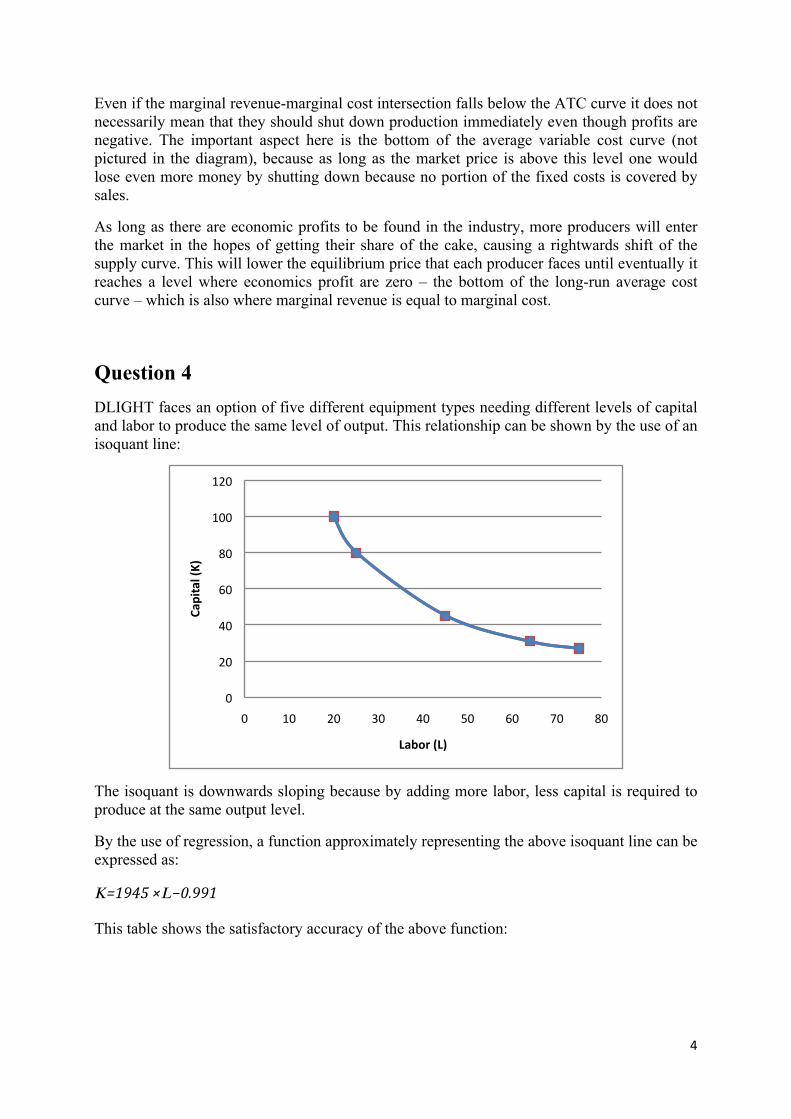
Question 4 DLIGHT faces an option of five different equipment types needing different levels of capital and labor to produce the same level of output. This relationship can be shown by the use of an isoquant line:

The isoquant is downwards sloping because by adding more labor, less capital is required to produce at the same output level.

By the use of regression, a function approximately representing the above isoquant line can be expressed as:

𝐾=1945  ×𝐿−0.991

This table shows the satisfactory accuracy of the above function:

0  

20  

40  

60  

80  

100  

120  

0   10   20   30   40   50   60   70   80  

Capital  (K)  

Labor  (L)  

5    

Labor  given   Capital  given   Capital  from  equation   Difference  20   100   99.91   0.09  25   80   80.09   0.09  45   45   44.73   0.27  64   31   31.55   0.55  75   27   26.96   0.04  

Question 5 We are given a price of labor (w) of USD 100 and a price of capital (r) of USD 140. The optimality condition for combining labor and capital is where the marginal rate of technical substitution (MRTS) – the ratio at which the two inputs can be substituted for each other keeping output the same – is equal to the absolute slope of the isocost line (𝑤𝑟).

From the previous question, we know that the relationship between the inputs is given by 𝐾=1945  ×𝐿−0.991. The MRTS is the absolute value of the derived function of this equation:

𝑀𝑅𝑇𝑆=  𝑑𝐾𝑑𝐿=  −1927.5×𝐿−1.991=1927.5×𝐿−1.991

Because L is a positive number, the absolute value of the derived function gives us:

𝑀𝑅𝑇𝑆=1927.5×𝐿−1.991.

We then set MRTS equal to 𝑤𝑟 to find the optimal input level of L:

1927.5×𝐿−1.991=  𝑤𝑟

1927.5×𝐿−1.991=  100140

𝐿=52.88

To find K we simply insert this level of L into the original equation:

𝐾=1945  ×52.88−0.991

𝐾=38.12

This holds true assuming that capital and labor are infinitely divisible.

Question 6

The optimality condition of combining labor and capital is when the isocost line (the line representing the different combinations possible at a given total cost) is tangent to the isoquant. That is because this will yield the cheapest combination of labor and capital producing the desired level of output.

6    

As seen in the above example, the green isocost line is tangent to the isoquant. The point of tangency is therefore when the two input factors are combined most efficiently. The red isocost line crosses the isoquant twice; therefore it would be possible to operate with these input levels. But seeing as the green isocost represents a lower total cost with the same output, operation at the intersections of the red isocost is not desirable. The purple isocost line has a lower total cost than the others. However, it never intercepts the isoquant so that the input combinations this represents never reaches the desired level of output. Therefore the point of tangency yields the optimal combination.

Question 7 The answer to question 5 stated that the optimal input levels are L = 52.88 and K = 38.12. However, seeing as DLIGHT can only choose from the five equipment types these are not possible to reach. The optimal levels are placed somewhere in between equipment types C and D, so one of these two would be the best choice.

According to calculations, D is slightly cheaper at the output level of one ton. The cost of D is:

𝑇𝐶𝐷=𝑤𝐿+𝑟𝐾=100  ×64+140  ×31=𝑈𝑆𝐷  10,740

While the cost of C is:

𝑇𝐶𝐶=𝑤𝐿+𝑟𝐾=100  ×45+140  ×45=𝑈𝑆𝐷  10,800

Because the cost difference is relatively small, other factors could also be taken into consideration when deciding which equipment to invest in. In favor of C is the fact that it is less reliable on labor, which is a positive thing because wages may be more prone to increase in the case of social reforms improving the general welfare of the population. There are, however, advantages on relying more on labor as equipment type D does. It can be considered

0  

2  

4  

6  

8  

10  

12  

0   1   2   3   4   5   6  

7    

easier (and cheaper) to replace labor than capital in a part of the world where spare parts may be hard to come by.

Therefore, if we were to give DLIGHT a final answer on the question of the most desirable equipment type we would go for D seeing as it is the cheapest one and as the old managerial economics saying states: “profit is God”.

Question 8 Cost-volume-profit analysis – also known as breakeven analysis – focuses on the quantity that the firm has to produce in order to break even, i.e. have zero profits. This quantity is found by dividing the fixed costs with the contribution margin per unit, so the formula for calculating the breakeven quantity can be expressed as:

𝑄𝐵=  𝑇𝐹𝐶(𝑃−𝐴𝑉𝐶)

This holds true because this gives the level of Q that will make 𝑄  ×(𝑃−𝐴𝑉𝐶) equal to and thereby covering the fixed costs.

In this case we are given a fixed cost of USD 250,000, a price per kg of USD 8 and variable costs of USD 2.5 per kg produced. Plugging these numbers into the equation, we find that:

𝑄𝐵=  250,000(8−2.5)=45,454.54  𝑘𝑔

The breakeven quantity is therefore 45.45 tons.

Revenue is price multiplied by quantity. In order to find the breakeven revenue, we therefore multiply the breakeven quantity by the given price:

𝐵𝑟𝑒𝑎𝑘𝑒𝑣𝑒𝑛  𝑟𝑒𝑣𝑒𝑛𝑢𝑒=𝑄𝐵×𝑃=45,454  𝑘𝑔×8𝑈𝑆𝐷𝑘𝑔

𝐵𝑟𝑒𝑎𝑘𝑒𝑣𝑒𝑛  𝑟𝑒𝑣𝑒𝑛𝑢𝑒=𝑈𝑆𝐷  363,636.36  

Question 9 When using the breakeven analysis, it is important to keep in mind that there are some underlying assumptions which must be made for the analysis to be applicable. First, prices and average variable costs must be constant (otherwise, we would obtain a nonlinear breakeven chart). This speaks against what we usually assume in microeconomic theory, namely that in order to sell more of a product, producers will have to lower prices; that is, we have a downward-sloping demand curve. In breakeven analysis, we have to disregard this principle.

Second, the assumption has to be made that the firm in question produces only one product or a constant mix of products. In the case of DLIGHT, a constant mix of products would implicate that the ratio of their sales of Exquisite Delight 80 g chocolate to their sales of bulk-package chocolates does not change, as this could change the fixed and/or variable cost scheme.

8    

A constant average variable cost implies a constant marginal cost at all levels of Q, meaning constant returns to scale in the industry. This is needed in order to obtain the linear shape of the TC curve in the breakeven chart. In microeconomics, we often assume that marginal cost will first decrease as Q grows (economies of scale) and later increase (diseconomies of scale). This microeconomic assumption would cause the TC curve to be of non-linear shape and possibly make it intersect the TR curve at more than one place, and this is the reason we assume no economies of scale in the breakeven analysis.

All in all, the above shows that the breakeven analysis has some significant shortcomings and cannot be applied to all cases. Also, in order to use the analysis it may be necessary to disregard or modify at least some of the assumptions normally made in microeconomic theory.

Question 10 The degree of operational leverage (DOL) measures the ratio of the firm’s fixed costs to variable costs. A high operational leverage – meaning that the relative amount of fixed costs is high – is associated with a higher risk. It puts pressure on the firm because it will have to reach a higher level of sales in order to break even or make profits. The advantage is that when the breakeven point is reached the firm makes a higher profit per unit sold (the contribution margin) than if operating with a lower degree of operational leverage. A higher degree of operational leverage can for example be obtained if a firm moves into a new production facility with a higher rent. This increases fixed costs, but the better facilities will likely improve the efficiency of the workers, thus lowering variable costs.

The degree of operational leverage is calculated by using the formula:

𝐷𝑂𝐿=  %∆𝜋%∆𝑄

9    

So the degree of operational leverage measures the responsiveness of profits to a change in the level of output. Rearranging, we find that:

𝐷𝑂𝐿=  𝑄  ×(𝑃−𝐴𝑉𝐶)𝑄  ×𝑃−𝐴𝑉𝐶−  𝑇𝐹𝐶

Therefore as fixed costs increase, the degree of operational leverage also increases. If a firm has no fixed costs so that the firm is not leveraged at all, the DOL will be equal to 1.

Inserting the known variables, we therefore find the degree of operational leverage to be:

𝐷𝑂𝐿=  100,000  ×8−2.5100,000  ×8−2.5−  250,000

𝐷𝑂𝐿=1.83

This means that a 1% increase in the level of output will yield a 1.83% increase in profits. A degree of operational leverage of 1.83 is not particular high, so DLIGHT is not very leveraged. Therefore, if DLIGHT is willing to take the risk of raising fixed costs to lower variable costs, for example moving into new and better facilities or purchasing new vehicles for transportation, they could improve their profits.

Question 11

Even though the equipment is able to operate for ten years it may not economically viable to keep it for the whole technical lifespan. The optimal economic lifespan is the number of periods that will yield the highest accumulated net present value – in other words how long the equipment’s contribution to revenue outweighs the economic cost of keeping the machine.

The schedule below sums up the calculations done when finding the optimal economic lifespan. The scrap value is the amount that the machinery could be sold for at the given time. Value loss (how much the equipment drops in value if kept for another year), interest loss (the interest you could gain by selling the machine and putting the money in the bank) and maintenance costs represent the costs of keeping the machine for one more year (thus a marginal cost). The MR column shows the revenue that will be gained by keeping the equipment another year. The NPV for each time is calculated by discounting the difference between marginal revenue and marginal cost back to the base year, and accumulated NPV is the sum of the NPV’s at a given time.

In the case of DLIGHT accumulated NPV is at its highest at the end of period 7; therefore this is the optimal economic lifespan and the company should sell the machinery at time 7.

t Scrap Value

loss Interest

loss Maint. costs

Total (MC) costs MR MR-MC NPV Acc NPV

0 1,000,000 1 900,000 100,000 150,000 250,000 500,000 800,000 300,000 260,870 260,870

10    

2 800,000 100,000 135,000 262,500 497,500 900,000 402,500 304,348 565,217 3 700,000 100,000 120,000 275,625 495,625 1,000,000 504,375 331,635 896,852 4 600,000 100,000 105,000 289,406 494,406 1,000,000 505,594 289,075 1,185,927 5 500,000 100,000 90,000 303,877 493,877 800,000 306,123 152,197 1,338,124 6 400,000 100,000 75,000 319,070 494,070 640,000 145,930 63,089 1,401,214 7 300,000 100,000 60,000 335,024 495,024 512,000 16,976 6,382 1,407,596 8 200,000 100,000 45,000 351,775 496,775 409,600 -87,175 -28,498 1,379,098

9 100,000 100,000 30,000 369,364 499,364 327,680 -

171,684 -48,803 1,330,295

10 0 100,000 15,000 387,832 502,832 262,144 -

240,688 -59,494 1,270,800

Question 12 Issuing of new share capital is a tool companies can use to increase their amount of share capital. The three most common ways to do this is through issuing of bonus shares, share capital increase with privileged subscription rights or share capital increase with free subscription rights.

Bonus shares do not increase the amount of capital in a company, but transfers capital from retained earnings into share capital, therefore the equity stays the same although the number of shares increases. An issuing of bonus shares does not increase the shareholder’s portion of equity but may increase his dividend, and is therefore more of a way to please shareholders than to finance investments.

A share capital increase with privileged subscription rights increases the number of shares, share capital and total equity. In addition existing shareholders have the opportunity to buy a number of new shares at the offered subscription price, the amount depending on their number of existing shares. Although this decreases the price per share, due to the subscription right the shareholders do not lose anything. If a shareholder does not use his subscription right, it can be sold and the buyer will be able to purchase a share at the new market price. A company can also raise capital by floating new shares on the free market, where anyone can buy them and there are no subscription rights. This is called share capital increase with free subscription. Other than the subscription differences it affects share capital and equity in much the same way. These are what we can call external financing because both of these raise equity and can therefore contribute to financing an investment.

Question 13 In order to examine the value and viability of an investment, the risk has to be considered. The risk can be divided into two subcategories: financial risk and business risk. The latter is typically linked to the industry’s market conditions. In order to assess business risk, several factors have to be taken into consideration, e.g. demand uncertainty, price fluctuations and availability of input factors (in the case of DLIGHT mainly cocoa), expansion opportunities, sales price volatility and others. The conditions in the particular market should also be considered (applying for instance the Porter’s Five Forces and PESTEL models).

For DLIGHT, the following assessment of business risk can be made:

11    

DLIGHT is heavily dependent on cocoa beans for production. As in every business that relies on agricultural products as a main input factor, there is always the possibility of considerable yearly price fluctuations of inputs due to either good or bad harvests. DLIGHT in particular, being an Ecuador-based company relying completely on a local network of cocoa bean producers, is facing this risk. If the cocoa bean harvest in Ecuador fails and prices therefore rise, DLIGHT cannot easily obtain cocoa beans from regions which have not experienced a bad harvest.

The same is the case if, say, political upheaval in Ecuador were to dramatically increase cocoa production prices for local farmers. Again, DLIGHT is dependent on its local supply network and would face this increase in prices, not being able to shift their own supply.

Apart from the risk of bad harvests, however, the market for cocoa beans should be relatively safe to navigate in for a company like DLIGHT, seeing as this market bears the characteristics of perfect competition and thus supplier strength is weak, which will make it harder for suppliers to push up prices and easier for DLIGHT to maintain input prices at a low level.

The demand side of the high-end chocolate market can be assumed to be fairly stable. DLIGHT supplies a luxury product (per definition), and as mentioned in the case material, the market for delicacy chocolate has grown to great extent since year 2000 in several key markets. There may even still be some unexploited potential in this market, seeing as customers and retailers show interest in new brands and varied origin.

As long as DLIGHT has a product that is desirable for customers even in comparison with the close-substitute products of other chocolate producers, the company should to be able to keep selling their chocolate at favorable prices. Since DLIGHT’s product is differentiated from other chocolate products, a price cut from a competing company will not necessarily force DLIGHT to cut prices as well. However, a general shift in customer taste from chocolate to other exclusive snack products could drive down prices and pose a threat to chocolate companies with a relatively small product variety like DLIGHT.

A last relevant subject to touch upon is the cost structure of the company, which can done by examining the degree of operating leverage (DOL), i.e. the relationship between fixed and variable costs. As previously mentioned, we assess that DLIGHT is not very leveraged, and therefore the business risk related to DLIGHT’s cost structure is also at a low level.

For these reasons, the level of business risk faced by DLIGHT and the industry is fairly low.

Question 14 When considering investing, one does not always know the exact future cash flows. Sometimes they may turn out as expected, but often conditions change unexpectedly. The idea of the real options approach is that as new information appears over time choices can be altered on whether not to invest or to invest differently. It thereby gives us a non-static view of the decision process.

Let us for example consider which real options there are if considering investing as a shareholder in DLIGHT. If the original perception of the risk is that there are equal chances of losing or gaining money, the decision tree could look something like this:

12    

This would yield an expected net present value of zero if the possible payoff is of an equal amount to the potential loss. It is therefore a rather risky investment, but the risk can be reduced via the real options approach. Say for example one was to wait a period to see if conditions changed. The decision tree might then look like this:

The conditions have now changed and there is a higher possibility of a loss than a gain. Therefore by waiting one might have avoided a possible loss. One reason for a change in circumstances could be the harvest going wrong, lowering the value of the firm.

Another example of the real options approach could be to hire a consultant to analyze and assess the probabilities of the different outcomes. In the example below, the consultant’s assessments are that because of for example the low business risk of DLIGHT previously mentioned, the probability of success is actually higher than the potential shareholder initially thought, causing the investment to be more attractive:

13    

Question 15 The discount rate applied is determined by the two risk parameters; business risk and financial risk. If both of these risks are high, the overall risk level is critical, and in that case a very high discount rate should be applied. If both risk levels are low the investment in itself is not that risky; however, because of the lack of financial gearing the Return on Equity (ROE) is not as high as it could be.

As explained in question 13, DLIGHT’s business risk is relatively low. The degree of operational leverage is not very high; the threat of suppliers driving up prices is low; and the demand for DLIGHT’s chocolates seems quite stable.

Looking at the financial risk, in this part of the assignment DLIGHT is considering raising money for the investment through issuing of new share capital (external financing). This raises equity without increasing debt, thereby lowering the debt-to-equity ratio and decreasing the financial risk.

Because both risk parameters are low, the discount rate applied will be low as well. We would estimate that a fair discount rate in this case would be approximately 12% or somewhere else between 10% and 15%.

However, later it is discussed whether DLIGHT should finance the investment through a loan. This would increase the debt-to-equity ratio and drive up financial risk, which would potentially cause the shareholders to require higher returns as the cost of debt goes up, increasing the discount rate applied. However, the company may benefit from the financial gearing causing the Return on Equity to increase, so taking up a loan instead of issuing new shares may be favorable.

14    

Question 16 The repayment schedule for DLIGHT looks like this:

t Outst. Interest Install PMT 0 800,000 784,000 1 752,578 48,000 47,422 -95,422 2 702,311 45,155 50,267 -95,422 3 649,029 42,139 53,283 -95,422 4 592,549 38,942 56,480 -95,422 5 532,680 35,553 59,869 -95,422 6 469,219 31,961 63,461 -95,422 7 401,951 28,153 67,268 -95,422 8 330,646 24,117 71,305 -95,422 9 255,063 19,839 75,583 -95,422

10 174,945 15,304 80,118 -95,422 11 90,020 10,497 84,925 -95,422 12 0 5,401 90,020 -95,422

The amount received in time 0 is less than the loan amount because of a 2% front-end fee. DLIGHT will have half-yearly payments of USD 95,422 over the six-year repayment of the loan.

In order to calculate the period effective interest rate one must find the internal rate of return of the payments. Using Microsoft Office Excel’s IRR function this yields a period effective interest rate of 6.37%. Having found this it is possible to calculate the annual effective interest by the use of the equation:

𝐴𝑛𝑛𝑢𝑎𝑙  𝑒𝑓𝑓𝑒𝑐𝑡𝑖𝑣𝑒  𝑖𝑛𝑡𝑒𝑟𝑒𝑠𝑡  𝑟𝑎𝑡𝑒=(1+𝐼𝑃𝑒𝑓𝑓)𝑛𝑜.𝑝𝑒𝑟𝑖𝑜𝑑𝑠  𝑝𝑒𝑟  𝑦𝑒𝑎𝑟−  1

So in this case the annual effective interest rate is:

𝐴𝑛𝑛𝑢𝑎𝑙  𝑒𝑓𝑓𝑒𝑐𝑡𝑖𝑣𝑒  𝑖𝑛𝑡𝑒𝑟𝑒𝑠𝑡  𝑟𝑎𝑡𝑒=(1+0.0637)2−  1

𝐴𝑛𝑛𝑢𝑎𝑙  𝑒𝑓𝑓𝑒𝑐𝑡𝑖𝑣𝑒  𝑖𝑛��𝑒𝑟 𝑒𝑠𝑡  𝑟𝑎𝑡𝑒=13.15%

The annual effective interest rate is higher than the nominal interest rate due to the 2% front-end fee as well as the effect of compounded half-yearly payments.

Question 17 One of the most important things to consider other than effective interest rate is how well the loan matches the investment. If the investment is expected to have a stable and relatively even cash flow throughout its life expectancy, an annuity loan where payments are equal will be best. On the other hand, if the investment is expected to produce a high cash flow in the beginning which diminishes over time a serial loan is best suited. This way the firm will pay equal installments every time, but higher payments in the beginning, making the later payments smaller. A third option is a bullet loan. This is optimal for investments that will not yield a sufficient cash flow until the very end, and one therefore avoids paying installments

15    

while waiting for the investment to pay off. If there is a period before an investment pays off, such as with products that require research or development, it is a good idea to get a loan with a grace period, a period when the firm only pays interest and no installments.

Another thing to consider is whether or not to lease the equipment instead of buying it. Leasing would allow the company to use the equipment without taking out a loan, but instead paying rent. This makes the financial gearing of the company lower, thus lowering its financial risk, which is good if they have a high business risk and may give them a better interest rate if they need to take out a loan for something else.

In the case of DLIGHT a serial loan would be preferable seeing as the revenue of the investment is large in the beginning, but decreases towards the end.

Question 18 Knowing the responsiveness to price changes as well as the quantity demanded for one given price, we can find the demand function by first calculating the price elasticity at this point.

𝜀𝑃=  %∆𝑄%∆𝑃

A 5% decrease in price causes a 10% increase in volumes sold:

𝜀𝑃=  10%−5%=  −2

Knowing the price elasticity for a given point, we can use the following formula to find the slope:

𝜀𝑃=  𝑃𝑄  ×  1𝑠𝑙𝑜𝑝𝑒

Inserting the known variables:

−2=  3500,000  ×  1𝑠𝑙𝑜𝑝𝑒

Isolating slope, this yields:

𝑠𝑙𝑜𝑝𝑒=  −31,000,000

Knowing that this describes the slope of a linear price function:

𝑠𝑙𝑜𝑝𝑒=  𝑃2−  𝑃1𝑄2−  𝑄1

We insert the slope and the known variables of P and Q as P2 and Q2 and replace Q1 with a 0 so that P1 represents the intersection of the Y-axis:

−31,000,000=  3−  𝑃𝑖𝑛𝑡.500,000−  0

Isolating the intersection of the Y-axis, it yields:

𝑃𝑖𝑛𝑡.=4.5

16    

Having calculated the slope and the intersection with the Y-axis, the demand function is therefore:

𝑷=�.�−��,���,���  ×𝑸

The MR function has the same intersection of Y and twice the slope of the demand function, so:

𝑴𝑹=�.�−����,���  ×𝑸

The functions will look like this:

Question 19

The demand curve faced by the individual firm, in this case DLIGHT, is not flat; therefore it cannot be perfect competition. Furthermore the market does not have a kinked demand curve either, because consumers are as sensitive to price increases as they are to price decreases, and is therefore not an oligopoly market. On the other hand, although there are no or few perfect substitutes for DLIGHT’s chocolate-covered nuts, there are many close substitutes both in the nut industry, the chocolate industry and the snack industry as a whole. Also the entry barriers in the industry are relatively low; one does not need a lot of big investments to get started although some are required.

These factors lead to the conclusion that this is a market of monopolistic competition. There are many firms, relatively low entry barriers and the products are to a certain degree similar, but still with some different attributes and variations in quality and varieties.

Because of the prevailing market form DLIGHT should be very careful about raising their prices as there are many close substitutes in this market form. Instead they may gain from competing in other ways, for example trying to differentiate themselves even more from the

0  

0.5  

1  

1.5  

2  

2.5  

3  

3.5  

4  

4.5  

5  

0   500000   1000000   1500000   2000000  

Price  

Quan=ty  

demand  

MR  

17    

other chocolate producers and thereby gaining an advantage on competitors who may have lower prices, but have a product less attractive in the eyes of the public.

Question 20 In question 18, the demand curve for DLIGHT was derived from information about how much the volume sold of Exquisite Delight 80 g chocolate would change (that is, a given percentage change in Q) in response to either a 5% increase or a 5% decrease in price (a given percentage change in P). The ratio of a change in Q to a change in P is more commonly known as the price elasticity of demand, or εP.

Price elasticity of demand is in other words a measurement of the responsiveness of the quantity demanded of a good to a change in its price. The relationship between the demand curve that DLIGHT faces and εP can be seen in the following illustration:

The point at which the firm maximizes its total revenue (TR) is exactly the midpoint of the demand curve. At this point |𝜀𝑃|=1, meaning that a 1% increase/decrease in price will lead to a 1% decrease/increase (accordingly) in volume sold. Demand is then said to be unitary elastic. In the case of DLIGHT unitary elasticity is found with a price of USD 2.25 (the middle of the curve – half of the price at the Y-axis intersection), at which the quantity demanded is 750,000 units.

The part of the demand curve that is above the midpoint is where |𝜀𝑃|>1, meaning that a 1% increase/decrease in price will lead to a more-than-1% decrease/increase in volume sold, and here demand is elastic. For DLIGHT this will be at a price level higher than USD 2.25.

18    

Correspondingly, the part of the demand curve below the midpoint is where |𝜀𝑃|<1, and demand is inelastic – and this is where DLIGHT would operate with prices lower than USD 2.25 per unit.

Firms want to be on the elastic part of their demand curves. If they operate at the inelastic portion they could always gain higher revenue by producing less and charging a higher price. Equally, by producing less it would likely lower their costs (although accumulated discounts might cause exceptions), so profits would increase by producing at the elastic portion. Because the accumulated discounts facing DLIGHT (which will be elaborated in the next question) take effect in the elastic portion this does not change anything.

The calculations earlier showed that the price elasticity at the price level where DLIGHT operates is -2, so as predicted DLIGHT is operating on the elastic portion of the demand curve.

Question 21 For quantities Q ≤ 400,000, the following average and marginal costs prevail:

𝑨𝑽𝑪=�−�.������𝑸

𝑻𝑽𝑪=𝑸×𝑨𝑽𝑪=�𝑸−�.������𝑸�

𝑴𝑪=𝒅𝑻𝑽𝑪𝒅𝑸=�−�.������𝑸 For quantities Q > 400,000, the following average variable costs and total variable costs prevail:

𝑨𝑽𝑪=�.�

𝑻𝑽𝑪=𝑸×𝑨𝑽𝑪=�.�𝑸 When the quantity increases from 400,000 to 400,001, there is a drop in total variable costs, likely due to accumulated discounts. At this point, MC = -39,998.5. When Q > 400,001:

𝑴𝑪=𝒅𝑻𝑽𝑪𝒅𝑸=�.�

0  

0.5  

1  

1.5  

2  

2.5  

0   100000   200000   300000   400000   500000   600000  

Price  

Quan=ty  

MC  

AVC  

MC  &  AVC  

19    

Instead of showing the MC at the level where the discount takes effect as a negative number, it can be illustrated as a ‘free’ amount for certain quantities. At Q = 400,001, TVC = 600,001.5. Using the cost structure of the lower quantities, =2𝑄−0.000001𝑄2 , total variable costs will be equal to USD 600,001.5 at Q = 367,545.65. Therefore, the output level 367,545.65 < Q < 400,000 will be undesirable to produce because total costs of production will be lowered as soon as levels of Q > 400,000 are reached. Question 22 As previously mentioned, the optimality condition is always at the point when MR = MC. The challenge in this case is that the MC curve has a gap because of the accumulated quantity discount taking place.

As seen in the illustration, the intersection of the MR and MC curves takes place after the accumulated discount has had an effect. Therefore the relevant portion of the MC curve is where:  𝑀𝐶=1.5 We know from question 18 that MR can be expressed as: 𝑀𝑅=4.5−61,000,000×𝑄  

We therefore set MR = MC to find the optimal quantity: 4.5−61,000,000×𝑄=1.5  

𝑄=500,000  Knowing the optimal quantity we insert this into the demand function to find the optimal price: 𝑃=4.5−31,000,000×500,000  

𝑃=3    

0  0.5  1  

1.5  2  

2.5  3  

3.5  4  

4.5  5  

0   100000   200000   300000   400000   500000   600000   700000  

Price  

Quan=ty  

MC  

MR  

20    

So DLIGHT optimizes production at an output level of 500,000 units of Exquisite Delight 80 g chocolate with a price of USD 3. As we know from question 18 this is the output level they are producing at and the price they are charging, so DLIGHT is optimizing. Question 23 Even though a price of USD 3 at which 500,000 units can be sold is optimal for DLIGHT under the given conditions, they may be able to improve profits even more if considering the use of other pricing strategies. The most obvious way of doing this would be through the use of price discrimination, i.e. charging different prices under circumstances not related to cost differences. It exists in the forms of first-degree, second-degree and third-degree price discrimination.

First-degree price discrimination implies that each unit is sold separately and that customers are charged the highest possible price they are willing to pay for each unit, capturing the entire consumer surplus. However, this is not really realistic in the case of DLIGHT because first-degree price discrimination is practically impossible other than in theory; in real life the closest thing to this type of price discrimination would be auctions. Second-degree price discrimination implies the price declining the larger quantities bought. Prices are typically charged in block quantities, so that the first prescribed amount of units has one price, the next block another price and so on, capturing some but not all consumer surplus. This strategy is, however, most efficient for products with easy-to-measure quantities, e.g. how many minutes people talk on the phone. DLIGHT may to a limited degree benefit from charging a lower per-unit price if people buy three 80 g chocolates than if they only buy one. This is basically what they are already doing with their sales of the larger, vacuum-packed bags which will likely have a lower per-unit price than the 80 g units.

0  

0.5  

1  

1.5  

2  

2.5  

3  

3.5  

4  

4.5  

5  

0   100000   200000   300000   400000   500000   600000   700000  

21    

Most relevant of the three is third-degree price discrimination, i.e. charging different prices in different markets thereby optimizing in both markets. The markets have to be separable so that a customer in one market cannot easily purchase the product cheaper in the other market. Separate markets refers not only to geographical differences but can also refer to for example different age groups being charged different prices for public transportation, cinemas etc. Furthermore, to uphold this type of pricing the company must be able to control the price (i.e. not operate in perfect competition, which DLIGHT does not), face different price elasticities at the same price and most importantly, the separation of markets has to be legal. Geographical separation of markets should definitely be something for DLIGHT to consider seeing as customers in a relatively wealthy country such as Luxembourg may be willing to purchase at a higher price than local customers in Ecuador.

There exist other pricing practices than price discrimination, all of which are not necessarily relevant in the case of DLIGHT. One pricing strategy we would recommend them to consider, however, is the so-called prestige pricing. Prestige pricing implies intentionally setting prices high in order to attract high-class customers, which may lead to a certain degree of loyalty from this segment. Seeing as DLIGHT’s chocolate-covered Brazil nuts are more of a fashionable snack than most ‘regular’ chocolates this seems possible. If they at the same time brand themselves well with the history of the company scribbled on the packets and mention their self-established Total Quality Control they may benefit from this pricing strategy.

Question 24 Income elasticity of demand is a measurement of the responsiveness of demand to a change in consumer income; if income rises by 1%, how much does it affect sales? It can be written as:

𝜀𝐼=  %∆𝑄%∆𝐼

The usual effect of an increase in income is an increase in quantities sold. However, this is not always the case. If an increase in income has a decreasing effect on sales the product is classified as an inferior good, meaning that it is a type of product that people will demand less of as they become wealthier. An example of a typical inferior good are canned products which are relatively cheap and will seem less desirable if one can suddenly afford goods of higher quality and nutrition. If the effect of an increase in income is positive, but relatively modest, the good is considered a normal good, while a great responsiveness to the change in income is typical for the last type of goods, luxuries. The elasticities of the three are typically defined as:

𝐼𝑛𝑓𝑒𝑟𝑖𝑜𝑟  𝑔𝑜𝑜𝑑:  𝜀𝐼<0

𝑁𝑜𝑟𝑚𝑎𝑙  𝑔𝑜𝑜𝑑:  0<𝜀𝐼<1

𝐿𝑢𝑥𝑢𝑟𝑦  𝑔𝑜𝑜𝑑:  𝜀𝐼>1

We would expect DLIGHT’s products to have fairly high income elasticities, classifying it as a luxury good. Chocolate-covered nuts are not essential for one’s survival, but rather a treat people will purchase in the case of more money than they really need. Likewise, if a person’s

22    

income was to go down it would most likely be one of the first excess expenses to get rid of, hence a great responsiveness to income changes. An estimated income elasticity of approximately 2 could be expected. As mentioned earlier, prestige pricing is a price strategy DLIGHT may want to consider, and their product being a luxury good emphasizes this point even more; a heavier targeting at the wealthier social segments may be of benefit.