UNIVERSITY OF CANTERBURY

HONOURS THESIS

Malware Detection with Malware Imagesusing Deep Learning Techniques

Author:Ke HE

Supervisor:Dong-Seong KIM

A thesis submitted in fulfillment of the requirementsfor the degree of Bachelor of Science with Honours

in the

Department of Computer Science and Software Engineering

October 18, 2018

i

UNIVERSITY OF CANTERBURY

AbstractDepartment of Computer Science and Software Engineering

Bachelor of Science with Honours

Malware Detection with Malware Images using Deep Learning Techniques

by Ke HE

Driven by economic benefits, the number of malware attacks is increasing signifi-cantly on a daily basis. Malware Detection Systems (MDS) is the first line of de-fence against malicious attacks, thus it is important for malware detection systemsto accurately and efficiently detect malware. Current MDS typically utilizes tra-ditional machine learning algorithms that require feature selection and extraction,which are time-consuming and error-prone. Conventional deep learning based ap-proaches use Recurrent Neural Networks (RNN) which is vulnerable to redundantAPI injection, thus we investigate the effectiveness of Convolutional Neural Net-works (CNN) against redundant API injection. We designed a malware detectionsystem that transforms malware files into image representations and classifies theimage representation with CNN. The CNN is implemented with spatial pyramidpooling layers (SPP) to deal with varying size input. We evaluate the effectivenessof SPP and image colour space (greyscale/RGB) by measuring the performance ofour system on both unaltered data and adversarial data with redundant API in-jected. Results show that naive SPP implementation is impractical due to memoryconstraints and greyscale imaging is effective against redundant API injection.

ii

Contents

1 Introduction 1

2 Background 32.1 Malware Detection Systems . . . . . . . . . . . . . . . . . . . . . . . . . 3

2.1.1 Signature-based Malware Detection . . . . . . . . . . . . . . . . 32.1.2 Heuristic-based Malware Detection . . . . . . . . . . . . . . . . 32.1.3 Cloud-based Malware Detection . . . . . . . . . . . . . . . . . . 42.1.4 Limitations and Beyond . . . . . . . . . . . . . . . . . . . . . . . 6

2.2 Deep Learning . . . . . . . . . . . . . . . . . . . . . . . . . . . . . . . . . 72.2.1 Artificial Neural Networks . . . . . . . . . . . . . . . . . . . . . 72.2.2 Convolutional Neural Network . . . . . . . . . . . . . . . . . . . 92.2.3 Recurrent Neural Network . . . . . . . . . . . . . . . . . . . . . 10

2.3 Deep Learning in Malware Detection . . . . . . . . . . . . . . . . . . . . 112.3.1 Recurrent Neural Networks . . . . . . . . . . . . . . . . . . . . . 112.3.2 Convolutional Neural Networks . . . . . . . . . . . . . . . . . . 11

3 Design 133.1 Preprocessing . . . . . . . . . . . . . . . . . . . . . . . . . . . . . . . . . 133.2 Classification . . . . . . . . . . . . . . . . . . . . . . . . . . . . . . . . . . 143.3 Evaluation . . . . . . . . . . . . . . . . . . . . . . . . . . . . . . . . . . . 15

4 Experiments 174.1 Dataset . . . . . . . . . . . . . . . . . . . . . . . . . . . . . . . . . . . . . 174.2 Experiment Setup . . . . . . . . . . . . . . . . . . . . . . . . . . . . . . . 174.3 Unaltered Samples . . . . . . . . . . . . . . . . . . . . . . . . . . . . . . 18

4.3.1 Time Measurements . . . . . . . . . . . . . . . . . . . . . . . . . 214.4 Results Comparison . . . . . . . . . . . . . . . . . . . . . . . . . . . . . . 214.5 Adversary Samples . . . . . . . . . . . . . . . . . . . . . . . . . . . . . . 22

5 Discussion 265.1 Findings . . . . . . . . . . . . . . . . . . . . . . . . . . . . . . . . . . . . 26

5.1.1 Colour Space . . . . . . . . . . . . . . . . . . . . . . . . . . . . . 265.1.2 Spatial Pyramid Pooling . . . . . . . . . . . . . . . . . . . . . . . 26

5.2 Limitations . . . . . . . . . . . . . . . . . . . . . . . . . . . . . . . . . . . 275.3 Future Work . . . . . . . . . . . . . . . . . . . . . . . . . . . . . . . . . . 27

6 Conclusion 29

Bibliography 31

A Raw Experiment Results 36A.1 Fixed width . . . . . . . . . . . . . . . . . . . . . . . . . . . . . . . . . . 36A.2 Fixed Ratio . . . . . . . . . . . . . . . . . . . . . . . . . . . . . . . . . . . 38A.3 Adversary Data . . . . . . . . . . . . . . . . . . . . . . . . . . . . . . . . 41

iii

A.3.1 RGB with Resnet50 . . . . . . . . . . . . . . . . . . . . . . . . . . 41A.3.2 Grayscale with Resnet50 . . . . . . . . . . . . . . . . . . . . . . . 43A.3.3 Grayscale with Plain Network . . . . . . . . . . . . . . . . . . . 44

iv

List of Figures

2.1 Signature of a network attack on Windows SMB protocol . . . . . . . . 42.2 An example of the difference between NN and 5-NN, using 2D points

and 3 classes. Coloured regions are decision boundaries [24]. . . . . . . 52.3 A feature space that cannot be partitioned by any plane is shown

on the left. The kernel function f (x, y) = (x, y, x2 + y2) turns the2-dimensional sample space into 3-dimensional space, where a hy-perplane can be fitted [29]. . . . . . . . . . . . . . . . . . . . . . . . . . . 7

2.4 Left: a biological neuron. Right: a computational neuron [36] . . . . . . 82.5 An example neural network with 3 inputs, 2 hidden layers of 4 neu-

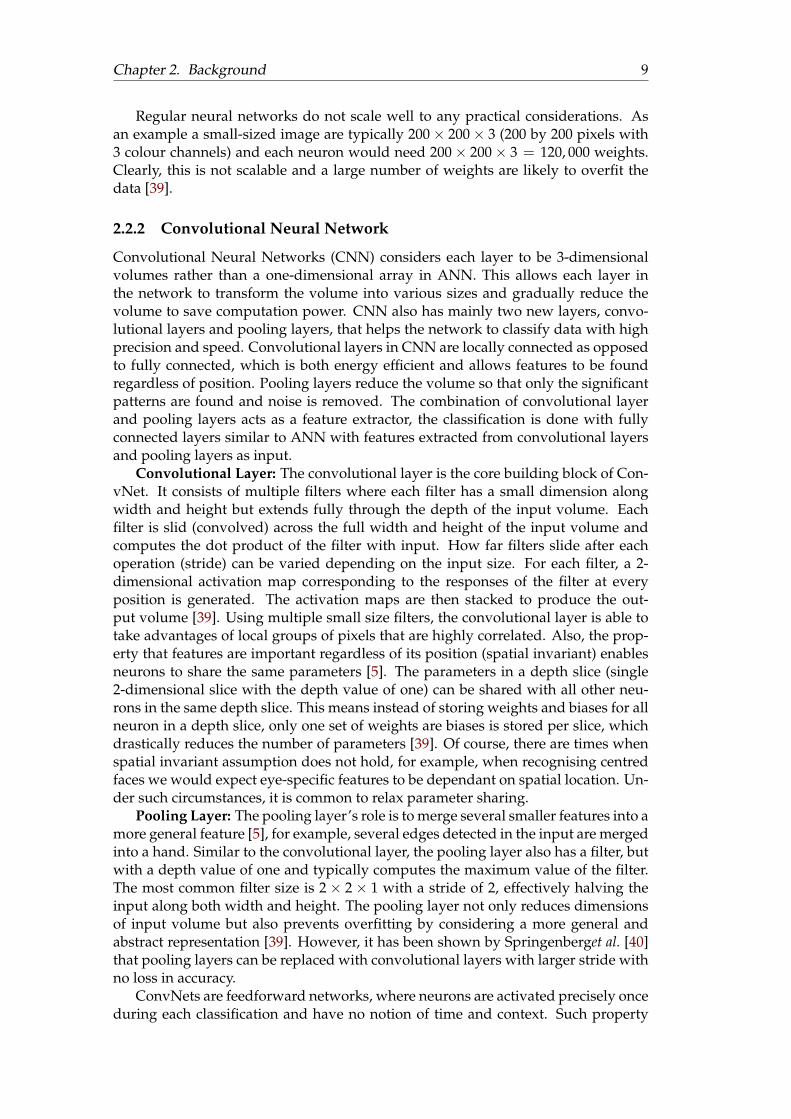
rons and one output layer [36] . . . . . . . . . . . . . . . . . . . . . . . . 82.6 Unfolding a Recurrent Neural Network. xt represents the input at

time t, ot represents the output at time t and st represents the memoryat time t, calculated based on xt and st−1. U, V, W are the sharedparameters of the network. [5] . . . . . . . . . . . . . . . . . . . . . . . . 10

3.1 The structure of malware detection system . . . . . . . . . . . . . . . . 133.2 A network with spatial pyramid pooling layer that pools feature maps

of any size into fixed-length (16+2+1=19 in this case) arrays [7]. . . . . 153.3 Left: the Resnet 50 model. Right: the 3 layer plain network. . . . . . . . 16

4.1 RoC Curves of models based on 3 layer plain network . . . . . . . . . . 194.2 RoC Curves of different models based on resnet50 network . . . . . . . 194.3 RoC Curves of different models based on 3 layer plain network . . . . 204.4 RoC Curves of different models based on resnet50 network . . . . . . . 204.5 RoC Curves of resnet50 model with RGB input and no SPP on adver-

sary inputs . . . . . . . . . . . . . . . . . . . . . . . . . . . . . . . . . . . 234.6 RoC Curves of resnet50 model with RGB input and no SPP on adver-

sary inputs . . . . . . . . . . . . . . . . . . . . . . . . . . . . . . . . . . . 234.7 RoC Curves of plain model with greyscale input and no SPP on ad-

versary inputs . . . . . . . . . . . . . . . . . . . . . . . . . . . . . . . . . 244.8 RoC Curves of resnet model with greyscale input and no SPP on ad-

versary inputs . . . . . . . . . . . . . . . . . . . . . . . . . . . . . . . . . 24

v

List of Tables

4.1 Summary of experimental parameters . . . . . . . . . . . . . . . . . . . 174.2 Summary of training parameters . . . . . . . . . . . . . . . . . . . . . . 174.3 Results of the experiment . . . . . . . . . . . . . . . . . . . . . . . . . . 18

A.1 Plain 3 layer network with RGB input and no SPP . . . . . . . . . . . . 36A.2 Plain 3 layer network with RGB input and SPP . . . . . . . . . . . . . . 36A.3 Plain 3 layer network with greyscale input and no SPP . . . . . . . . . 36A.4 Plain 3 layer network with greyscale input and SPP . . . . . . . . . . . 37A.5 Resnet50 network with RGB input and no SPP . . . . . . . . . . . . . . 37A.6 Resnet50 network with RGB input and SPP . . . . . . . . . . . . . . . . 37A.7 Resnet50 network with Greyscale input and no SPP . . . . . . . . . . . 38A.8 Resnet50 network with Greyscale input and SPP . . . . . . . . . . . . . 38A.9 Plain 3 layer network with RGB input and no SPP . . . . . . . . . . . . 38A.10 Plain 3 layer network with RGB input and SPP . . . . . . . . . . . . . . 39A.11 Plain 3 layer network with greyscale input and no SPP . . . . . . . . . 39A.12 Plain 3 layer network with greyscale input and SPP . . . . . . . . . . . 39A.13 Resnet50 network with RGB input and no SPP . . . . . . . . . . . . . . 40A.14 Resnet50 network with RGB input and SPP . . . . . . . . . . . . . . . . 40A.15 Resnet50 network with greyscale input and no SPP . . . . . . . . . . . 40A.16 Resnet50 network with greyscale input and SPP . . . . . . . . . . . . . 41A.17 Input file saturated by 10% with NOPs . . . . . . . . . . . . . . . . . . . 41A.18 Input file saturated by 20% with NOPs . . . . . . . . . . . . . . . . . . . 41A.19 Input file saturated by 30% with NOPs . . . . . . . . . . . . . . . . . . . 42A.20 Input file saturated by 40% with NOPs . . . . . . . . . . . . . . . . . . . 42A.21 Input file saturated by 50% with NOPs . . . . . . . . . . . . . . . . . . . 42A.22 Input file saturated by 10% with NOPs . . . . . . . . . . . . . . . . . . . 43A.23 Input file saturated by 20% with NOPs . . . . . . . . . . . . . . . . . . . 43A.24 Input file saturated by 30% with NOPs . . . . . . . . . . . . . . . . . . . 43A.25 Input file saturated by 40% with NOPs . . . . . . . . . . . . . . . . . . . 44A.26 Input file saturated by 50% with NOPs . . . . . . . . . . . . . . . . . . . 44A.27 Input file saturated by 10% with NOPs . . . . . . . . . . . . . . . . . . . 44A.28 Input file saturated by 20% with NOPs . . . . . . . . . . . . . . . . . . . 45A.29 Input file saturated by 30% with NOPs . . . . . . . . . . . . . . . . . . . 45A.30 Input file saturated by 40% with NOPs . . . . . . . . . . . . . . . . . . . 45A.31 Input file saturated by 50% with NOPs . . . . . . . . . . . . . . . . . . . 46

vi

List of Abbreviations

malware malicious softwareAV Anti-VirusAPI Application Programming InterfaceMDS Malware Detection SystemNN Nearest NeighbourkNN k Nearest NeighbourNBC Naive Bayes ClassifierSVM Support Vector MachineSPP Spatial Pyramid PoolingANN Artificial Neural NetworkCNN Convolutional Neural NetworkRNN Recurrent Neural NetworkRGB Red Green BlueNOP No OPeration

1

1 Introduction

Recent advances in hardware and software technologies have made digital devicesextremely powerful. Individuals and co-operations rely heavily on servers and com-puters to exchange and process information over the internet on a daily basis. It isestimated that there are 3.5 billion internet users as of 2017 and continues to growrapidly [1]. With a promising future ahead for the digital technologies industry,comes severe consequences. Driven by economic benefits, digital devices are underconstant threat of malicious software (malware).

Malware is an umbrella term for any software that intends to violate the confi-dentiality, integrity and availability of any digital device or system [2]. Attackerstypically utilise a wide range of malware, such as viruses, worms and Trojan horsesto steal confidential information, hijack computers, crash servers and many othermalicious activities. Such malicious activities could potentially cost the global com-munity 500 billion in total [3] and worldwide cyber-security spending is estimatedto reach 86.4 billion [4]. In order to protect individuals and large corporations fromsuch a catastrophe, it is important to ensure their digital devices and systems areused in a safe and secure environment.

The first line of defence against malicious attacks is malware detection system.They are distributed by anti-virus (AV) vendors to examine whether a file is mali-cious or benign. Traditional malware detection systems are based on shallow ma-chine learning algorithms (the term "shallow machine learning" or "traditional ma-chine learning" both refers to machine learning algorithms that are not deep learn-ing, e.g. decision trees, support vector machines and naive Bayes classifier). Theperformance of traditional machine learning algorithms relies heavily on the qualityof features extracted, however, feature selection and extraction are extremely time-consuming, error-prone and requires a high level of knowledge in the field. The nextgeneration of machine learning algorithms, deep learning, has become very popu-lar in recent times due to its ability to automatically extract sophisticated, high-levelfeatures that lead to high accuracy [5].

Current deep learning based malware detection systems are mostly based on Re-current Neural Networks (RNN) with API calls and machine instructions as inputand have been shown to have high accuracy. However, RNNs can be vulnerable toadversarial attacks where the attacker mimics the RNN used in the MDS based onthe input and output and use an adversarial RNN to add redundant API calls. Thefile with redundant API calls injected can easily bypass RNN detection [6]. The ro-bustness and effectiveness of using RNN in malware detection are still questionable.

The goal of this project is to investigate the resilience of Convolution NeuralNetwork (CNN) against redundant API injection. We theorise that adding redun-dant API calls corresponds to a distortion or translation of malware features in theimage space, which the CNN can still find. To achieve this task, we first transformthe input file into an image and train our CNN to learn the features/textures of theimage. A major problem is that conventional CNN takes fixed size inputs, but mal-ware files can come in drastically different sizes, thus we deploy Spatial PyramidPooling (SPP) [7] to make our CNN take inputs of arbitrary size.

Chapter 1. Introduction 2

The rest of this report is organised as follows: Chapter 2 provides backgroundof shallow and deep machine learning algorithms used in malware detection sys-tems, Chapter 3 showcases the design of our proposed malware detection systemand the respective rationale behind them, Chapter 4 examines the performance ofour proposed malware detection system, Chapter 5 discusses our finding from theexperiment as well as any further work and limitations. Finally, we conclude thisreport in Chapter 6.

3

2 Background

2.1 Malware Detection Systems

Malware detection systems have made a series of transformations from the earlysignature-based detection to the modern cloud-based detection. This section givesa brief summary of signature-based and heuristic-based malware detection systemswhile giving an in-depth analysis of traditional machine learning algorithms usedin cloud-based malware detection.

2.1.1 Signature-based Malware Detection

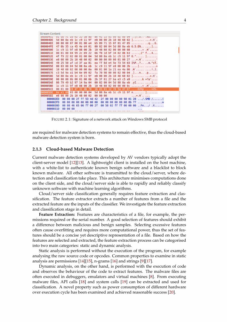
Early anti-malware vendors (e.g., Kingsoft, MacAfee and Symantec) commonly usedsignatures to identify malware [8]. A signature is a unique sequence of bytes exhib-ited by known malware samples and extracted by experts. An example of a networkattack signature is shown in Figure 2.1. Detection was done by simply checkingwhether the file contains any known malware signatures. Signature-based detec-tion is able to identify malware with an extremely small error rate and false positiverate of below 0.1% [9] but it is prone to countermeasures such as polymorphism,metamorphism and code obfuscation. The process of signature extraction is verytime-consuming and error-prone. On average it takes 54 days between a new mal-ware’s release and its detection [8] and fast-spreading malware such as viruses andworms would have already caused severe damage by the time malicious signaturesare found. Due to such limitations, the focus of identifying malware was shifted tobe based on heuristics rather than signatures.

2.1.2 Heuristic-based Malware Detection

Heuristic-based malware detection is a slight improvement of the signature-baseddetection. Instead of extracting a unique signature which only covers one variant ofa malware type [9], a set of heuristics are used. An ideal set of heuristics is composedof rules and patterns that sufficiently describe features belonging to all variants ofthe same type of malware yet not falsely matched on benign software [10]. An inputfile is matched against a collection of malicious heuristics to determine its malevo-lence. This method is able to cover a range of malware samples with a single set ofheuristics thus dramatically the reduces the workload of heuristic engineers. How-ever, heuristics do not come for free and requires large amounts of manual labourfor extraction, which was made infeasible by the rise of malware creation tool-kits.

Malware creation tool-kits are designed so that even someone with no program-ming knowledge can develop their own malware. This causes a rapid growth inthe number of new malware samples (200,000 new samples per day [11]) makingmanual extraction of heuristics infeasible. The growing malware sample size hasalso taken a toll on the client’s disk space, as it is not possible to store all heuristicson client machines. A more scalable architecture and intelligent detection algorithm

Chapter 2. Background 4

FIGURE 2.1: Signature of a network attack on Windows SMB protocol

are required for malware detection systems to remain effective, thus the cloud-basedmalware detection system is born.

2.1.3 Cloud-based Malware Detection

Current malware detection systems developed by AV vendors typically adopt theclient-server model [12][13]. A lightweight client is installed on the host machine,with a white-list to authenticate known benign software and a blacklist to blockknown malware. All other software is transmitted to the cloud/server, where de-tection and classification take place. This architecture minimises computations doneon the client side, and the cloud/server side is able to rapidly and reliably classifyunknown software with machine learning algorithms.

Cloud/server side classification generally requires feature extraction and clas-sification. The feature extractor extracts a number of features from a file and theextracted feature are the inputs of the classifier. We investigate the feature extractionand classification stage in detail.

Feature Extraction: Features are characteristics of a file, for example, the per-missions required or the serial number. A good selection of features should exhibita difference between malicious and benign samples. Selecting excessive featuresoften cause overfitting and requires more computational power, thus the set of fea-tures should be a concise yet descriptive representation of a file. Based on how thefeatures are selected and extracted, the feature extraction process can be categorisedinto two main categories: static and dynamic analysis.

Static analysis is performed without the execution of the program, for exampleanalysing the raw source code or opcodes. Common properties to examine in staticanalysis are permissions [14][15], n-grams [16] and strings [9][17].

Dynamic analysis, on the other hand, is performed with the execution of codeand observes the behaviour of the code to extract features. The malware files areoften executed in debuggers, emulators and virtual machines [8]. From executingmalware files, API calls [18] and system calls [19] can be extracted and used forclassification. A novel property such as power consumption of different hardwareover execution cycle has been examined and achieved reasonable success [20].

Chapter 2. Background 5

Both static and dynamic analysis has its own advantages and disadvantages.Static analysis is able to perform a comprehensive analysis of malware by exploringall code paths, but static analysis’ focus on source code made it vulnerable to codeobfuscation and encryption. Dynamic analysis is resilient to obfuscation by focusingon the file’s behaviour, but unable to examine edge cases that are hidden in the soft-ware. Due to the limitations of the static and dynamic analysis, malware detectionsystems often combine the two in practice to perform hybrid analysis [21], whichprovides a more comprehensive coverage of features.

Classification: Once features from malware file and benign files are extracted,it is up to machine learning algorithms to learn each sample so that it is able toclassify unseen files. The features extraction process transforms a file into a point inan n-dimensional feature space, where n is the number of features extracted, and theclassification process aims to segment the feature space into multiple sections basedon the training data, where each section contains the maximum possible numberof points belonging to the same category. Popular classification algorithms that wewill examine include Nearest Neighbour, Naive Bayes Classifier and Support VectorMachine.

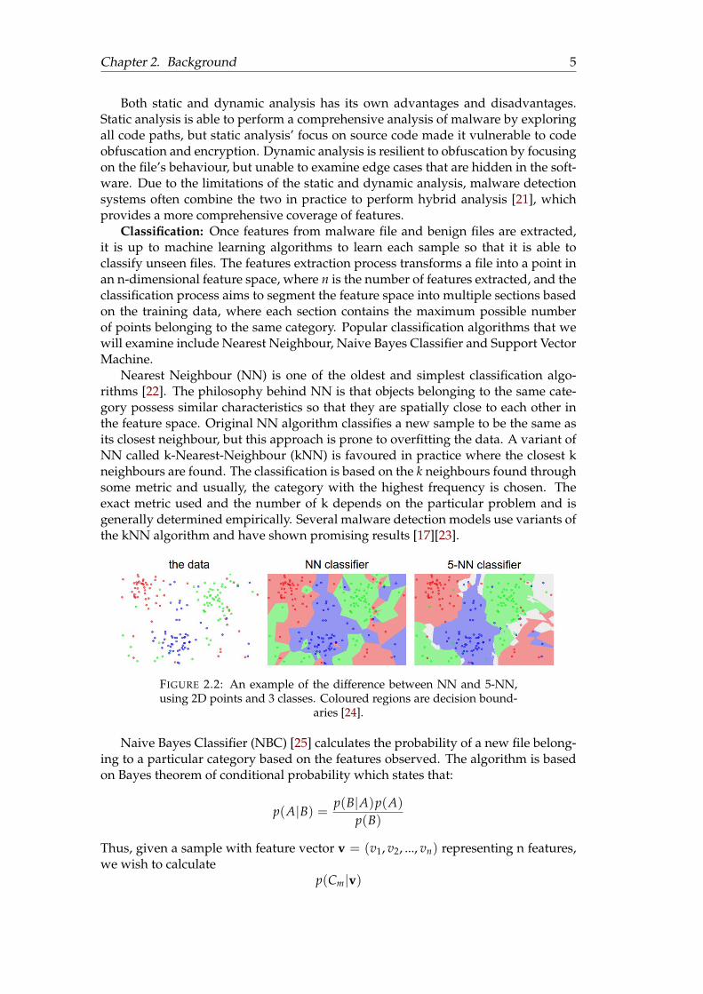
Nearest Neighbour (NN) is one of the oldest and simplest classification algo-rithms [22]. The philosophy behind NN is that objects belonging to the same cate-gory possess similar characteristics so that they are spatially close to each other inthe feature space. Original NN algorithm classifies a new sample to be the same asits closest neighbour, but this approach is prone to overfitting the data. A variant ofNN called k-Nearest-Neighbour (kNN) is favoured in practice where the closest kneighbours are found. The classification is based on the k neighbours found throughsome metric and usually, the category with the highest frequency is chosen. Theexact metric used and the number of k depends on the particular problem and isgenerally determined empirically. Several malware detection models use variants ofthe kNN algorithm and have shown promising results [17][23].

FIGURE 2.2: An example of the difference between NN and 5-NN,using 2D points and 3 classes. Coloured regions are decision bound-

aries [24].

Naive Bayes Classifier (NBC) [25] calculates the probability of a new file belong-ing to a particular category based on the features observed. The algorithm is basedon Bayes theorem of conditional probability which states that:

p(A|B) = p(B|A)p(A)

p(B)

Thus, given a sample with feature vector v = (v1, v2, ..., vn) representing n features,we wish to calculate

p(Cm|v)

Chapter 2. Background 6

Where Cm is m possible categories to be classified. Using Bayes’ Theorem, the aboveequation can be transformed as

p(Cm|v) =p(Cm)p(v|Cm)

p(v)

Note that the denominator is a constant, therefore only the numerator is of interest.The numerator is equivalent to the joint probability model p(Cm, v1, v2, ..., vn). Usingrepeated definition of conditional probability and the naive assumption that featuresv1, v2, ...vn are all conditionally independent, the numerator can be written as

p(Cm, v1, v2, ..., vn) = p(v1|v2, ..., vn, Cm)p(v2, ..., vn, Cm)

= ...= p(v1|v2, ..., vn, Cm)p(v2, ..., vn, Cm)...p(vn|Cm)p(Cm)

Due to conditional independence,p(vi|vi+1, ..., vn, Cm) = p(vi|Cm)

Thus,p(v1|v2, ..., vn, Cm)...p(vn|Cm)p(Cm) = p(v1|Cm)p(v2|Cm)...p(Cm)

= p(Cm)n

∏i=1

p(vi|Cm)

We have assumed independence of features when using NBC, but it has been em-pirically shown to be optimal even when the independence assumption is violatedby a large margin [26]. This observation has made NBC applicable across numerousdomains. Various malware detection systems have used NBC for classification andachieved good success [14][27].

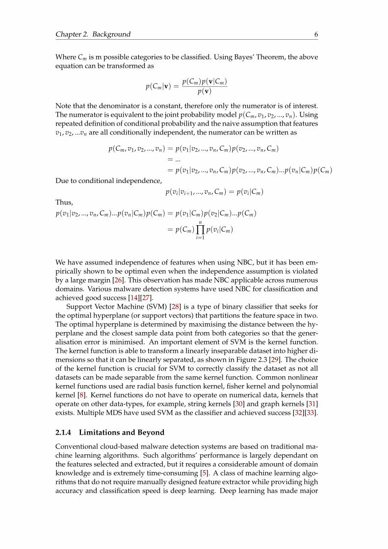
Support Vector Machine (SVM) [28] is a type of binary classifier that seeks forthe optimal hyperplane (or support vectors) that partitions the feature space in two.The optimal hyperplane is determined by maximising the distance between the hy-perplane and the closest sample data point from both categories so that the gener-alisation error is minimised. An important element of SVM is the kernel function.The kernel function is able to transform a linearly inseparable dataset into higher di-mensions so that it can be linearly separated, as shown in Figure 2.3 [29]. The choiceof the kernel function is crucial for SVM to correctly classify the dataset as not alldatasets can be made separable from the same kernel function. Common nonlinearkernel functions used are radial basis function kernel, fisher kernel and polynomialkernel [8]. Kernel functions do not have to operate on numerical data, kernels thatoperate on other data-types, for example, string kernels [30] and graph kernels [31]exists. Multiple MDS have used SVM as the classifier and achieved success [32][33].

2.1.4 Limitations and Beyond

Conventional cloud-based malware detection systems are based on traditional ma-chine learning algorithms. Such algorithms’ performance is largely dependant onthe features selected and extracted, but it requires a considerable amount of domainknowledge and is extremely time-consuming [5]. A class of machine learning algo-rithms that do not require manually designed feature extractor while providing highaccuracy and classification speed is deep learning. Deep learning has made major

Chapter 2. Background 7

FIGURE 2.3: A feature space that cannot be partitioned by any plane isshown on the left. The kernel function f (x, y) = (x, y, x2 + y2) turnsthe 2-dimensional sample space into 3-dimensional space, where a

hyperplane can be fitted [29].

break-through across multiple domains such as image recognition, speech recogni-tion and natural language processing [5]. Future cloud-based malware detectionsystems are highly likely to deploy deep learning algorithms at the cloud end forreliable and responsive detection and classification. We introduce deep learning andexamine current deep learning techniques applied in malware detection and otherrelated fields in the next section.

2.2 Deep Learning

The history of deep learning can be traced back to as early as the 1940s. Due tolimited computation power and inexperienced training strategies at the time, earlydeep learning algorithms such as aritificial neural networks nearly always resultedin a locally optimal solution and convergence is not guaranteed. It was not until2006 when Hinton et al. [34] proposed backpropagation, an efficient way of trainingand tuning the network, causing deep learning algorithms to be in favour [35].

Deep learning’s success is largely due to the absence of manually designed fea-ture extractor. Deep learning algorithms are able to automatically discover featuresor representations that are needed for classification straight from raw data. In otherwords, the feature extractor is designed by the algorithm itself. Such feature ex-tractors take less time, are less error-prone and most importantly, are able to extractintricate high dimensional features which humans cannot think of [5].

2.2.1 Artificial Neural Networks

Artificial Neural Networks (ANN) or connectionist systems lays the foundation ofmodern deep learning algorithms and were originally inspired by modelling thebiological neural system. The basic building blocks of the biological neural systemis a neuron, connected by synapses. Each neuron receives input signals from itsdendrites, then the input is processed by the cell nucleus and outputs signals alongits axon via synapses. The outputted signal is then received by dendrites of otherneurons. The computational model of a neuron is an extremely simplified version ofthe biological neuron: dendrites and axons are mapped to the input and output of

Chapter 2. Background 8

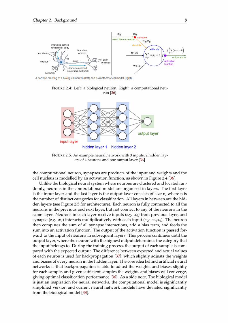
FIGURE 2.4: Left: a biological neuron. Right: a computational neu-ron [36]

FIGURE 2.5: An example neural network with 3 inputs, 2 hidden lay-ers of 4 neurons and one output layer [36]

the computational neuron, synapses are products of the input and weights and thecell nucleus is modelled by an activation function, as shown in Figure 2.4 [36].

Unlike the biological neural system where neurons are clustered and located ran-domly, neurons in the computational model are organised in layers. The first layeris the input layer and the last layer is the output layer consists of size n, where n isthe number of distinct categories for classification. All layers in between are the hid-den layers (see Figure 2.5 for architecture). Each neuron is fully connected to all theneurons in the previous and next layer, but not connect to any of the neurons in thesame layer. Neurons in each layer receive inputs (e.g. x0) from previous layer, andsynapse (e.g. w0) interacts multiplicatively with each input (e.g. w0x0). The neuronthen computes the sum of all synapse interactions, add a bias term, and feeds thesum into an activation function. The output of the activation function is passed for-ward to the input of neurons in subsequent layers. This process continues until theoutput layer, where the neuron with the highest output determines the category thatthe input belongs to. During the training process, the output of each sample is com-pared with the expected output. The difference between expected and actual valuesof each neuron is used for backpropagation [37], which slightly adjusts the weightsand biases of every neuron in the hidden layer. The core idea behind artificial neuralnetworks is that backpropagation is able to adjust the weights and biases slightlyfor each sample, and given sufficient samples the weights and biases will converge,giving optimal classification performance [36]. As a side note, The biological modelis just an inspiration for neural networks, the computational model is significantlysimplified version and current neural network models have deviated significantlyfrom the biological model [38].

Chapter 2. Background 9

Regular neural networks do not scale well to any practical considerations. Asan example a small-sized image are typically 200× 200× 3 (200 by 200 pixels with3 colour channels) and each neuron would need 200× 200× 3 = 120, 000 weights.Clearly, this is not scalable and a large number of weights are likely to overfit thedata [39].

2.2.2 Convolutional Neural Network

Convolutional Neural Networks (CNN) considers each layer to be 3-dimensionalvolumes rather than a one-dimensional array in ANN. This allows each layer inthe network to transform the volume into various sizes and gradually reduce thevolume to save computation power. CNN also has mainly two new layers, convo-lutional layers and pooling layers, that helps the network to classify data with highprecision and speed. Convolutional layers in CNN are locally connected as opposedto fully connected, which is both energy efficient and allows features to be foundregardless of position. Pooling layers reduce the volume so that only the significantpatterns are found and noise is removed. The combination of convolutional layerand pooling layers acts as a feature extractor, the classification is done with fullyconnected layers similar to ANN with features extracted from convolutional layersand pooling layers as input.

Convolutional Layer: The convolutional layer is the core building block of Con-vNet. It consists of multiple filters where each filter has a small dimension alongwidth and height but extends fully through the depth of the input volume. Eachfilter is slid (convolved) across the full width and height of the input volume andcomputes the dot product of the filter with input. How far filters slide after eachoperation (stride) can be varied depending on the input size. For each filter, a 2-dimensional activation map corresponding to the responses of the filter at everyposition is generated. The activation maps are then stacked to produce the out-put volume [39]. Using multiple small size filters, the convolutional layer is able totake advantages of local groups of pixels that are highly correlated. Also, the prop-erty that features are important regardless of its position (spatial invariant) enablesneurons to share the same parameters [5]. The parameters in a depth slice (single2-dimensional slice with the depth value of one) can be shared with all other neu-rons in the same depth slice. This means instead of storing weights and biases for allneuron in a depth slice, only one set of weights are biases is stored per slice, whichdrastically reduces the number of parameters [39]. Of course, there are times whenspatial invariant assumption does not hold, for example, when recognising centredfaces we would expect eye-specific features to be dependant on spatial location. Un-der such circumstances, it is common to relax parameter sharing.

Pooling Layer: The pooling layer’s role is to merge several smaller features into amore general feature [5], for example, several edges detected in the input are mergedinto a hand. Similar to the convolutional layer, the pooling layer also has a filter, butwith a depth value of one and typically computes the maximum value of the filter.The most common filter size is 2× 2× 1 with a stride of 2, effectively halving theinput along both width and height. The pooling layer not only reduces dimensionsof input volume but also prevents overfitting by considering a more general andabstract representation [39]. However, it has been shown by Springenberget al. [40]that pooling layers can be replaced with convolutional layers with larger stride withno loss in accuracy.

ConvNets are feedforward networks, where neurons are activated precisely onceduring each classification and have no notion of time and context. Such property

Chapter 2. Background 10

FIGURE 2.6: Unfolding a Recurrent Neural Network. xt representsthe input at time t, ot represents the output at time t and st representsthe memory at time t, calculated based on xt and st−1. U, V, W are the

shared parameters of the network. [5]

made ConvNets perform well in image classification tasks where features are spa-tially invariant, but poorly in natural language processing and speech recognitiontasks due to the order and context of the words matters significantly.

2.2.3 Recurrent Neural Network

Recurrent neural networks (RNN) are designed to recognise patterns in sequentialdata, which made them favourable in natural language processing tasks. The designphilosophy of RNN is that the order of inputs contains information as well as theinputs. The overall structure of RNN is similar to CNN, both have an input layer,an output layer and hidden layers. What is different is that RNN’s hidden layernot only considers the input at the current step but also the previous states of thesystem by recursively activating itself. The hidden layers have a "memory" of whathappened previously. The structure of a common RNN is shown in Figure 2.6 [5].

Unfortunately, training the network has proven to be problematic [35]. Memo-rising long-term behaviour of the system is difficult because the back propagatedgradients either grows or shrinks at each time step, causing the gradient to eitherexplode or vanish. As all neural networks rely on gradients to adjust its weightsand biases, a gradient of 0 or infinity makes the network untrainable. This phe-nomenon is largely due to information passes through many multiplicative stagesduring RNN. Similar to compound interest, an interest rate slightly higher than onecan become unimaginably large [41].

Long Short-Term Memory networks (LSTMs) [42] are a widely used variant ofRNNs that fixes the exploding/vanishing gradient problem by having a more com-plicated memory unit. The memory units in LSTM have its own weights and biasesthat are learning alongside with RNN and are able to decide whether the new inputis ignored or impact current memory or forget existing memory (e.g. contexts in anew paragraph or section may be irrelevant to previous paragraph/section). To fur-ther reduce the exploding/vanishing rate, the LSTM memory unit adds the inputwith previous states rather than multiply the two. This naively simple change ofcalculation has proven to be quite effective.

Chapter 2. Background 11

2.3 Deep Learning in Malware Detection

Deep learning has made major advances across multiple domains such as imagerecognition, speech recognition, natural language processing and many more [5]. Ithas even extended into more recreational domains such as automatically generatingdank memes [43]. It is not surprising that some of the latest MDS uses deep learningtechniques to achieve high accuracy and speed. This section explores current deeplearning methods adopted in malware detection system.

2.3.1 Recurrent Neural Networks

Recurrent neural networks (RNN) have been the first choice of most deep learningbased malware detection systems. The task of malware detection is analogous to textclassification, which RNNs excel at. Designers of RNN-based MDS believe the se-quential information contained within machine instructions and API calls extractedfrom the malware is useful to detect malware, just like text classification [44][45]. Atypical RNN based malware detection system encodes each API call/instruction as aone-hot vector of dimension M, where M is the number of total API calls/instructions.Given API calls/instructions are labelled from 0 to M− 1, for an API call/instructionlabelled i, all numbers in the vector are 0 except for index i, where the number is1. A sequence of embedded API calls is gathered into a matrix and is fed into theRNN for classification. Several variations of RNN have been evaluated [46], show-ing LSTM network with max pooling and logistic regression as classification outper-forms character-level CNN.

A major drawback of RNN is its ability to only learn one language environmentor structure. Attackers can exploit this weakness by predicting the language that aparticular RNN based malware detection system has learned with a substitute RNNand use another RNN to generate adversarial code to bypass malware detection sys-tems. A simple yet effective way of generating adversarial code is to insert irrelevantand redundant API calls, and most of the generated adversarial code is able to by-pass RNN detection [6]. The effectiveness of RNN in malware detection is uncertain.

2.3.2 Convolutional Neural Networks

Convolutional neural network (CNN) extracts hierarchical local features from datasamples regardless of location, thus frequently used for image classification. Never-theless, we theorise CNN is a better candidate for malware detection compared toRNN. In the image space, adding redundant API calls or machine instructions cor-responds to a translation or distortion of features, which a CNN can be trained torecognise. As a trivial example, a hand in an image is still a hand regardless of itsposition or orientation, but a hand in a text segment can be a noun or a verb depend-ing on the context. With RNN-based MDS, attackers can change the context to trickthe MDS to think the word "hand" is a noun when it should be a verb by adding"the" in front of it. CNN on the other hand, adding words around the image woulddistort or translate the feature, which the CNN can easily recognise.

Unfortunately, classifying malware with CNN have not been extensively dis-cussed in literature. Yuan et. al. proposed an MDS that extracts a set of features withhybrid analysis and use CNN to classify the extracted feature vectors [47]. Simplyusing just a CNN with API calls or machine instructions were rarely done. We sus-pect it is mainly due to two reasons: 1. Finding a good method of representing a

Chapter 2. Background 12

malware file as an image is difficult. 2. It is difficult to deal with files/images ofvarious sizes.

13

3 Design

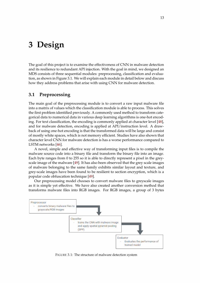
The goal of this project is to examine the effectiveness of CNN in malware detectionand its resilience to redundant API injection. With the goal in mind, we designed anMDS consists of three sequential modules: preprocessing, classification and evalua-tion, as shown in Figure 3.1. We will explain each module in detail below and discusshow they address problems that arise with using CNN for malware detection.

3.1 Preprocessing

The main goal of the preprocessing module is to convert a raw input malware fileinto a matrix of values which the classification module is able to process. This solvesthe first problem identified previously. A commonly used method to transform cate-gorical data to numerical data in various deep learning algorithms is one-hot encod-ing. For text classification, the encoding is commonly applied at character level [48],and for malware detection, encoding is applied at API/instruction level. A draw-back of using one-hot encoding is that the transformed data will be large and consistof mostly white spaces, which is not memory efficient. Studies have also shown thatcharacter level CNN for malware detection is has a worse performance compared toLSTM networks [46].

A novel, simple and effective way of transforming input files is to compile themalware source code into a binary file and transform the binary file into an image.Each byte ranges from 0 to 255 so it is able to directly represent a pixel in the grey-scale image of the malware [49]. It has also been observed that the grey scale imagesof malware belonging to the same family exhibits similar layout and texture, andgrey-scale images have been found to be resilient to section encryption, which is apopular code obfuscation technique [49].

Our preprocessing model chooses to convert malware files to greyscale imagesas it is simple yet effective. We have also created another conversion method thattransforms malware files into RGB images. For RGB images, a group of 3 bytes

FIGURE 3.1: The structure of malware detection system

Chapter 3. Design 14

represents each pixel in the output image, corresponding to red, green and bluecolour channels respectively. The bytes are processed line by line and the outputpixels are placed sequentially in a row, with the width of the output image fixed toan arbitrary number of 1920 pixels (it is the width of monitor screen). Any newlinecharacters are ignored and if the last few bytes cannot fill the entire line, it is paddedwith black pixels.

The reason behind transforming into RGB images is that we theorise it will ex-ihibit better performance. CNN considers each input as a volume, for greyscaleimage of size n × m, the input volume is n × m × 1, whereas for RGB images, thevolume would be n/

√3×m/

√3× 3. This shortens the distance between each pair

of bytes and allows CNN to find more complex patterns in the malware file.

3.2 Classification

The classification module takes the transformed image from the preprocessor anduses that image to train the CNN. Malware files come in various sizes, howevertypical CNN only accept a fixed size input. There are several ways to modify theinput to a fixed size, described below.

• Gilbert [50] proposed a malware detection system based on greyscale imagerepresentation of malware and down-sampled all malware samples to 32× 32pixels.

• CNN based image classification methods either crop or warp the original im-age to the required size [7].

• Athiwaratkun et al. [46] limited the input to be 1014 characters in the character-level CNN and padded shorter ones with zeros.

Modifying the input image is not ideal for malware detection, as it is prone toinformation loss before detection stage. Attackers can deliberately put maliciouscode in places that are potentially going to be removed before classification, thusbypassing detection system. For example, if the detection system only takes the first32 × 32 (1024) pixels as an input, the attacker can simply add the malicious codeafter 1024 pixels, bypassing detection.

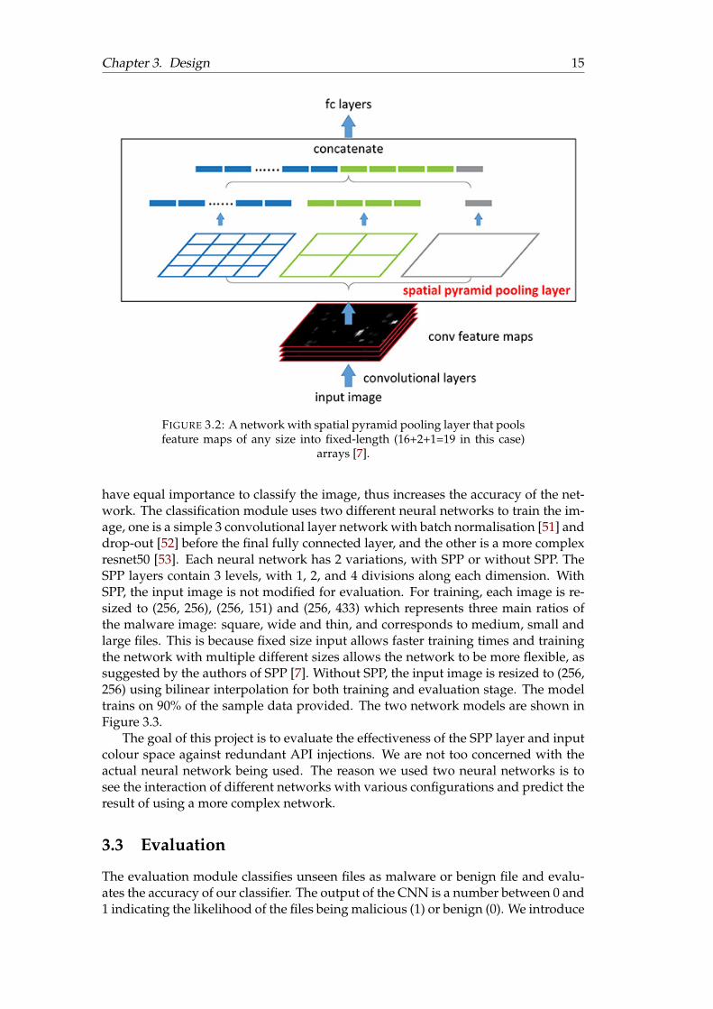
Manipulating the input file is not ideal, therefore can we design the CNN sothat it accepts input of various sizes? The answer is yes and the method is spatialpyramid pooling (SPP) [7]. The two main parts of a typical CNN are convolutionallayers and fully connected layers. The convolutional layer operates in a sliding win-dow manner and the output is dependent on the size of the input. It is only thefully connected layers that require a fixed size input to output a fixed size output ofthe categories. SPP operates in between the last convolutional layer and fully con-nected layer and divides the features maps from the last convolutional layer intomultiple levels and multiple subsections. Each subsection in each level undergoesmax pooling to extract the most dominant feature and each feature is concatenatedinto a fixed-length output array for the fully connected layers. The SPP layer al-lows the neural network to take an input image of arbitrary size and outputs a fixedsized feature array for the fully connected layers. The operation of SPP is shown inFigure 3.2.

Before training our neural network, we preprocess the images by rescaling allpixel from 0 to 255 into 0 to 1 and apply sample-wise normalization. These prepro-cessing steps are commonly done in order to make sure each feature in the image

Chapter 3. Design 15

FIGURE 3.2: A network with spatial pyramid pooling layer that poolsfeature maps of any size into fixed-length (16+2+1=19 in this case)

arrays [7].

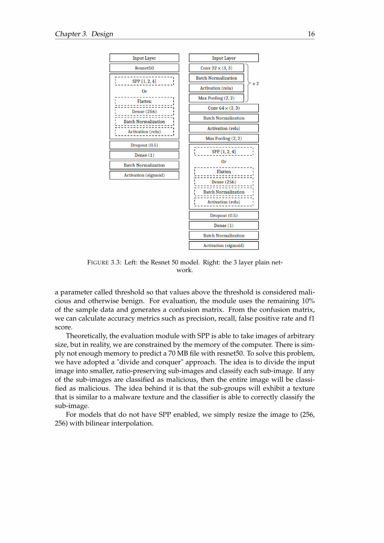
have equal importance to classify the image, thus increases the accuracy of the net-work. The classification module uses two different neural networks to train the im-age, one is a simple 3 convolutional layer network with batch normalisation [51] anddrop-out [52] before the final fully connected layer, and the other is a more complexresnet50 [53]. Each neural network has 2 variations, with SPP or without SPP. TheSPP layers contain 3 levels, with 1, 2, and 4 divisions along each dimension. WithSPP, the input image is not modified for evaluation. For training, each image is re-sized to (256, 256), (256, 151) and (256, 433) which represents three main ratios ofthe malware image: square, wide and thin, and corresponds to medium, small andlarge files. This is because fixed size input allows faster training times and trainingthe network with multiple different sizes allows the network to be more flexible, assuggested by the authors of SPP [7]. Without SPP, the input image is resized to (256,256) using bilinear interpolation for both training and evaluation stage. The modeltrains on 90% of the sample data provided. The two network models are shown inFigure 3.3.

The goal of this project is to evaluate the effectiveness of the SPP layer and inputcolour space against redundant API injections. We are not too concerned with theactual neural network being used. The reason we used two neural networks is tosee the interaction of different networks with various configurations and predict theresult of using a more complex network.

3.3 Evaluation

The evaluation module classifies unseen files as malware or benign file and evalu-ates the accuracy of our classifier. The output of the CNN is a number between 0 and1 indicating the likelihood of the files being malicious (1) or benign (0). We introduce

Chapter 3. Design 16

FIGURE 3.3: Left: the Resnet 50 model. Right: the 3 layer plain net-work.

a parameter called threshold so that values above the threshold is considered mali-cious and otherwise benign. For evaluation, the module uses the remaining 10%of the sample data and generates a confusion matrix. From the confusion matrix,we can calculate accuracy metrics such as precision, recall, false positive rate and f1score.

Theoretically, the evaluation module with SPP is able to take images of arbitrarysize, but in reality, we are constrained by the memory of the computer. There is sim-ply not enough memory to predict a 70 MB file with resnet50. To solve this problem,we have adopted a "divide and conquer" approach. The idea is to divide the inputimage into smaller, ratio-preserving sub-images and classify each sub-image. If anyof the sub-images are classified as malicious, then the entire image will be classi-fied as malicious. The idea behind it is that the sub-groups will exhibit a texturethat is similar to a malware texture and the classifier is able to correctly classify thesub-image.

For models that do not have SPP enabled, we simply resize the image to (256,256) with bilinear interpolation.

17

4 Experiments

The following experiments are done in order to evaluate the performance of thedesigned MDS against redundant API injection. The experiments mainly examinethe effect of the input colour space, complexity of CNN and spatial pyramid poolingon the performance of our network, with some additional experiments done to proveor disprove our theory. For simplicity, we only consider two distinct levels for eachparameter. Table 4.1 shows the configurable parameters and its respective levels.

Parameter Level 1 Level 2Preprocessing Greyscale RGBArchitecture 3 layer plain CNN Resnet50SPP No SPP SPP with bin sizes (1,2,4)

TABLE 4.1: Summary of experimental parameters

4.1 Dataset

The dataset used for the experiment is kindly provided by Korea University from theAndro-dumpsys study [21]. The dataset consists of 906 malicious binary files from13 malware families, including smishing and spy applications. The benign files area variety of popular applications with high rankings downloaded from GooglePlaystore. The benign files are checked by VirusTotal [54] to ensure it is indeed benign,and this resulted in 1776 benign files.

4.2 Experiment Setup

The setup used for conducting the following experiments is a 64 bit Linux mint18.3 Desktop with a quad-core Intel© CoreTM i7-4770 at 3.40GHz, 16GB RAM andGeForce GTX 750 Ti. The program is written in Python 3.5 with Keras and Tensor-flow as backend.

The model is trained with 90% of the collected sample, with batch size 16, 150iterations and 20 epochs respectively. A summary of training parameters is shownin Table 4.2. Once the training is done, all weights are saved for evaluation later.

Batch Size 16Epochs 20

Training Malware Size 815Training Benign Size 1598

Iterations 150

TABLE 4.2: Summary of training parameters

Chapter 4. Experiments 18

4.3 Unaltered Samples

Before we evaluate the resilience of the design MDS against adversary result, it isimportant to evaluate the performance on normal, unaltered data. There is no pointhaving an MDS that is resilient to adversary data but performs poorly with normaldata. The precision and recall of all eight classifiers with a threshold value of 0.5 areshown in Table 4.3, confusion matrix and accuracy metrics for all experiments doneare listed in Appendix A.

Network Precision RecallGreyscale plain noSPP 0.950 0.620Greyscale plain SPP 0.295 0.670Greyscale resnet noSPP 0.468 0.791Greyscale resnet SPP 0.190 0.044RGB plain noSPP 0.666 0.110RGB plain SPP 0.156 0.084RGB resnet noSPP 0.542 0.703RGB resnet SPP 0.0625 0.066

TABLE 4.3: Results of the experiment

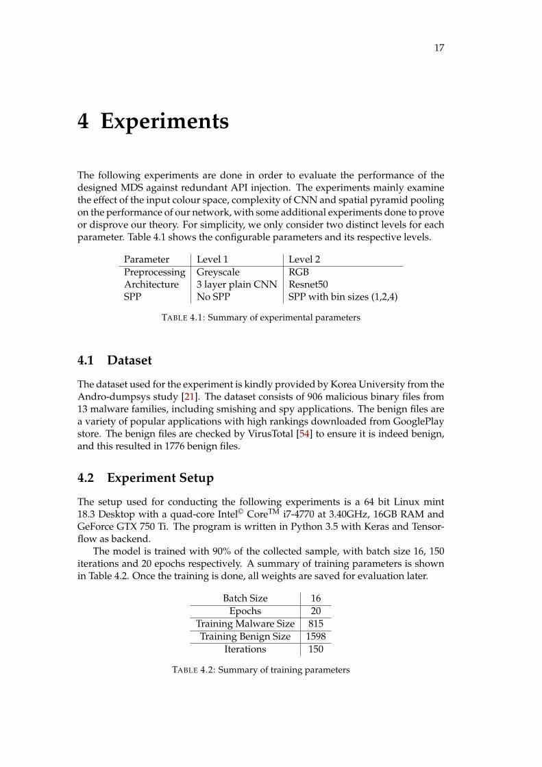
From Table 4.3, we observe that a plain network with greyscale and no SPPhave the highest precision but a relatively low recall, while a resnet50 network withgreyscale and no SPP have the highest recall but low precision.

We can also see that SPP performs poorly compared to the no SPP counterpart.The reason could be the threshold value of 0.5 is too high for SPP. Since we are usinga divide and conquer approach, the entire file is classified as malicious if a sub-imageis malicious, with a threshold of 0.5, large images are extremely likely to be classifiedas malicious even if they are benign. We vary the threshold value from 0.1 to 0.9 in0.1 increments to examine each model in more detail.

Figure 4.1 and 4.2 shows the RoC curve of each model with various thresholdsrespectively.

The results show the resnet50 network has better performance when the inputimage is in RGB colour space, and the plain network performs better with greyscaleimages. We theorise this is due to RGB images contains more sophisticated patternsdue to bytes/pixels being closer together in the input volume, such patterns are tocomplex for a shallow 3 plain layer network to capture, but the resnet50 networkcan.

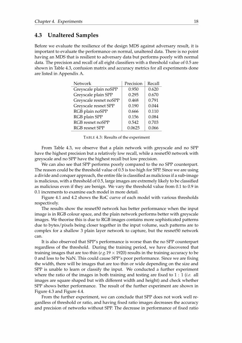
It is also observed that SPP’s performance is worse than the no SPP counterpartregardless of the threshold. During the training period, we have discovered thattraining images that are too thin (e.g.19× 1920) results in the training accuracy to be0 and loss to be NaN. This could cause SPP’s poor performance. Since we are fixingthe width, there will be images that are too thin or wide depending on the size andSPP is unable to learn or classify the input. We conducted a further experimentwhere the ratio of the images in both training and testing are fixed to 1 : 1 (i.e. allimages are square shaped but with different width and height) and check whetherSPP shows better performance. The result of the further experiment are shown inFigure 4.3 and Figure 4.4.

From the further experiment, we can conclude that SPP does not work well re-gardless of threshold or ratio, and having fixed ratio images decreases the accuracyand precision of networks without SPP. The decrease in performance of fixed ratio

Chapter 4. Experiments 19

0 0.2 0.4 0.6 0.8 10

0.2

0.4

0.6

0.8

1

False Positive Rate

True

Posi

tive

Rat

e

rgb falsergb true

grayscale falsegrayscale true

FIGURE 4.1: RoC Curves of models based on 3 layer plain network

0 0.2 0.4 0.6 0.8 10

0.2

0.4

0.6

0.8

1

False Positive Rate

True

Posi

tive

Rat

e

rgb falsergb true

grayscale falsegrayscale true

FIGURE 4.2: RoC Curves of different models based on resnet50 net-work

Chapter 4. Experiments 20

0 0.2 0.4 0.6 0.8 10

0.2

0.4

0.6

0.8

1

False Positive Rate

True

Posi

tive

Rat

ergb falsergb true

grayscale falsegrayscale true

FIGURE 4.3: RoC Curves of different models based on 3 layer plainnetwork

0 0.2 0.4 0.6 0.8 10

0.2

0.4

0.6

0.8

1

False Positive Rate

True

Posi

tive

Rat

e

rgb falsergb true

grayscale falsegrayscale true

FIGURE 4.4: RoC Curves of different models based on resnet50 net-work

Chapter 4. Experiments 21

images is likely due to the varying width causes the textures to change for each sam-ple, thus decreasing the accuracy. To see this, consider a simple binary case whereeach bit alternates from 0 to 1 (i.e.101010). With width 2, the image will have onevertical line of zeroes and another vertical line of ones. However, with width 3, theimage will have a checkered pattern. Note that this effect is different from addingredundant pixels in the image when adding a 1 to our toy example, a vertical line ofones can still be seen at width 2.

We hypothesise the devastating failure of SPP was due to the divide and conquerapproach. The problem that arises with the divide and conquers approach is split-ting a large malware texture into two sub-images which the classifier is not able toidentify and having only a subset of malware features in a sub-image is not sufficientto classify the sub-image as malicious. As an analogy, if we wish to classify whetheran image is a face using the divide and conquer method, we might pick up an eyein one image, but only having an eye is not sufficient to classify the sub-image as aneye.

In hindsight, the "divide and conquer" approach is theoretically fraud and des-tined to fail. The "divide and merge" might be a better solution and is worth explor-ing. "Divide and merge" divides the image into smaller sub-images, pools dominatefeatures from each sub-image and concatenate it together to form a more concise im-age. Then, the neural network classifies the merged image. This way, we are able tocombine smaller malicious/benign features to form a complete image of a malware.However this approach does not solve the problem of dividing a malware featureinto multiple parts, and more experiments need to be done in order to evaluate thesignificance of splitting malware feature in practice.

4.3.1 Time Measurements

The plain network takes on average 10 minutes to train one epoch, with 20 epochsit takes 2 hours and 40 minutes, evaluation of each sample takes on average 0.28seconds. The resnet50 model takes 1 hour and 28 minutes to train one epoch, andwith 20 epochs it takes 29 hours 20 minutes to train. The evaluation time for eachsample takes 0.41 seconds on average. RGB and greyscale input does not affect thetraining time to a significant degree, and models with SPP takes 3 times longer totrain as we are training the same images at 3 different sizes.

4.4 Results Comparison

The Andro-Dumpsys [21] MDS, which uses the same dataset as us, extracts a com-prehensive set of features and characteristics to classify malware. Some of the mainfeatures that Andro-Dumpsys examines are serial numbers, API sequence calls, per-missions and memory acquisition. A large majority of the processing is done under2.8GHz Intel Xeon X5660 with 8GB RAM. The paper reported only 8 benign filesare classified as malicious and 16 malware classified as benign, this results in 0.45%false positive rate and 1.77% false negative rate. The accuracy of Andro-Dumpsys issignificantly higher compared to our model, however, such high accuracy comes ata cost of processing power. Andro-Dumpsys comprehensively analyses many fea-tures of the malware, which takes on average 74.18 seconds per megabyte to detectmalware. Our model does most of the processing during the training stage and thebest model only takes on average 0.41 seconds to evaluate each malware samplesince all samples are transformed into a fixed size.

Chapter 4. Experiments 22

Andro-Dumpsys has high accuracy but it is extremely slow. Our model is muchfaster than Andro-Dumpsys but with less accuracy. The accuracy of our detectionsystem can be easily improved by fine-tuning the network and use a more advancednetwork, but this is not the main goal of this project. Nevertheless, we have shownthat using convolutional neural networks can drastically improve the time need fordetection.

4.5 Adversary Samples

The goal of the experiments is to investigate our MDS’s resilience to redundant APIinjection. As preliminary results have shown, SPP does not work well in normalclassification tasks due to large variations in malware image size and our faulty ap-proach to solve the problem. Thus in the following experiments, we ignore modelswith SPP and only investigate the performance resizing malware images with bilin-ear interpolation. We investigate whether bilinear interpolation is able to preservefeatures after resizing. For example, an eye in a high-quality image is still distin-guishable when the image is compressed to a few kilobytes.

The adversary malware samples are generated as close to reality as possible. Onan Intel x86 CPU, there are two different types of NOP operations with either 1byte or multiple bytes ranging from 2 to 9 bytes [55]. To keep things simple weonly inject single-byte NOP instruction (0x90) into the binary file. The method forinjection NOP is simple, after each byte we add a NOP with a probability of 10%.This means the length of the images will increase by 10% on average. There areother ways of injecting NOPs, such as splitting 10% of the file size into n differentredundant chunks and inject such chunks at various places. For this experiment, weonly examine the effect of randomly adding NOP after each byte.

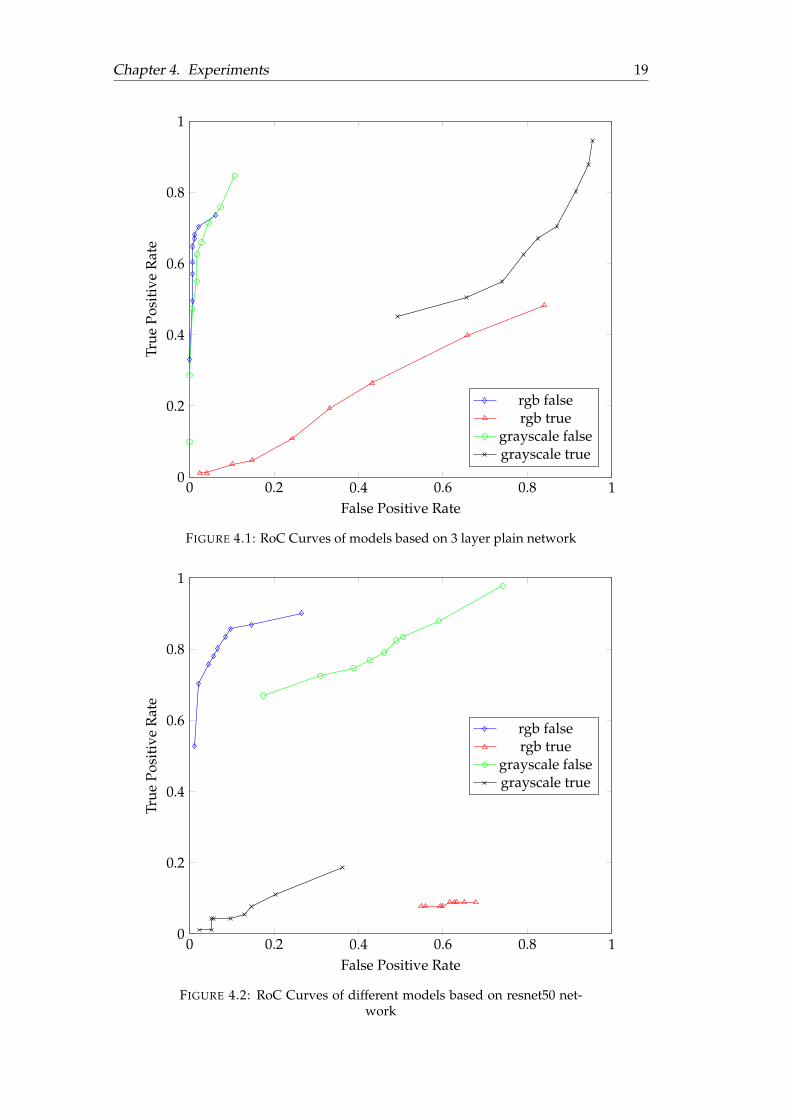
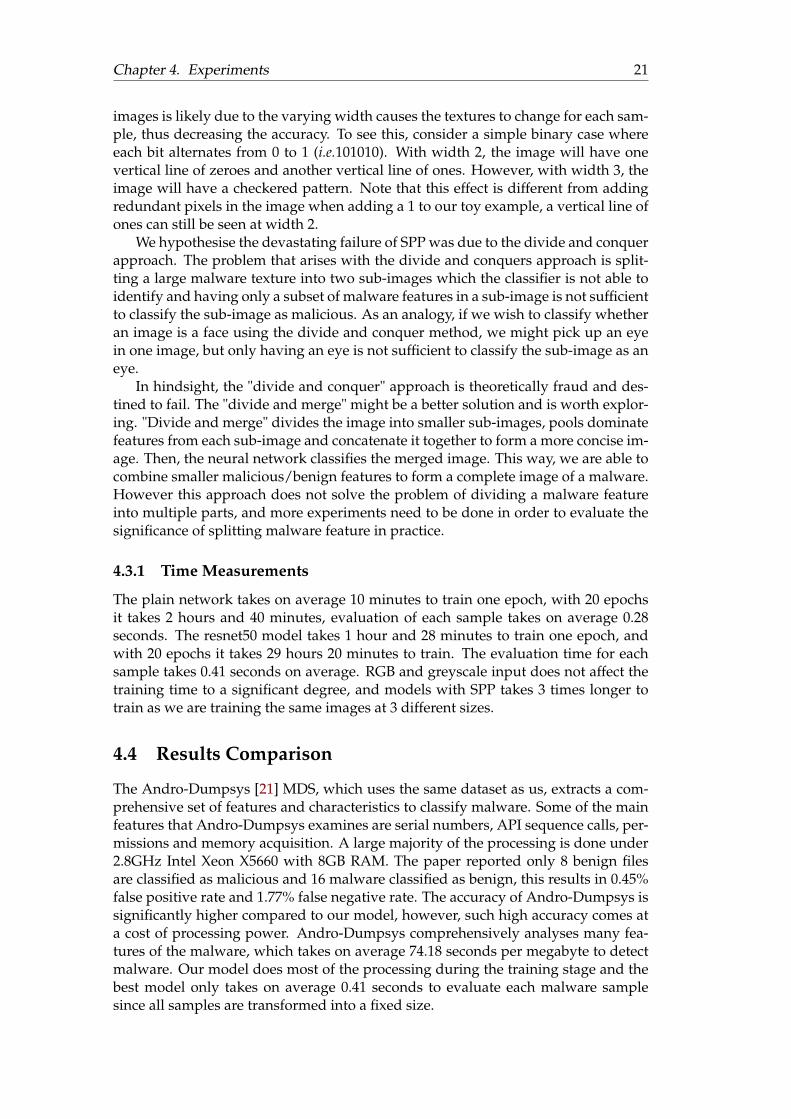
The model we wish to examine first is the resnet50 model with RGB input and noSPP. This is because the model has the highest f1 score overall on sample data (SeeAppendix A for complete metric). We evaluated the performance of the model onadversary samples that are fixed width and fixed ratio, the result is shown in Figure4.5.

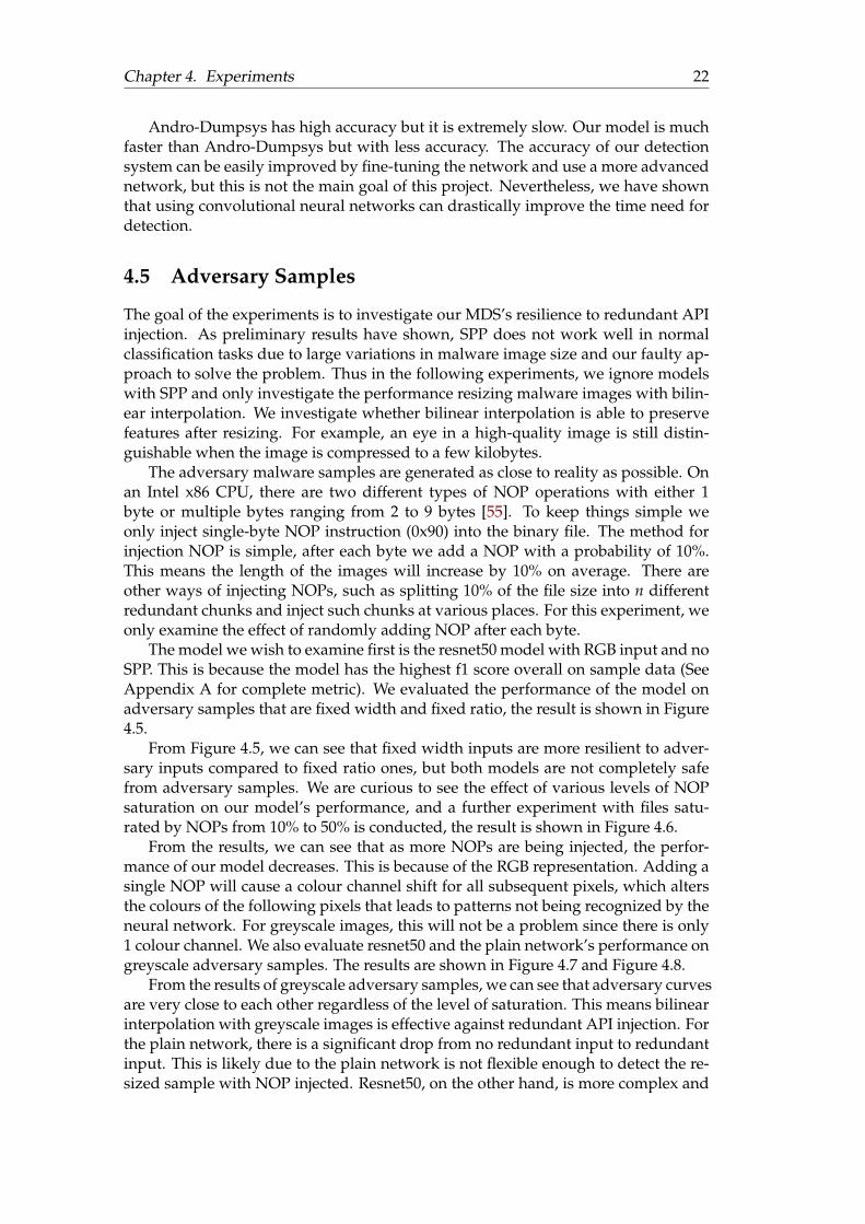
From Figure 4.5, we can see that fixed width inputs are more resilient to adver-sary inputs compared to fixed ratio ones, but both models are not completely safefrom adversary samples. We are curious to see the effect of various levels of NOPsaturation on our model’s performance, and a further experiment with files satu-rated by NOPs from 10% to 50% is conducted, the result is shown in Figure 4.6.

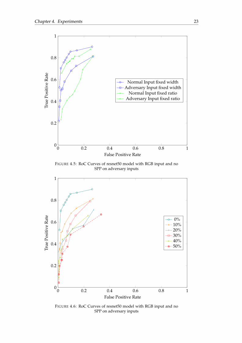
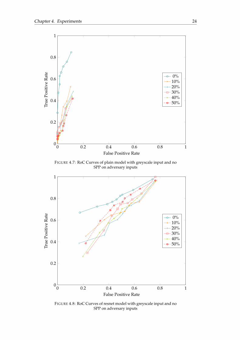
From the results, we can see that as more NOPs are being injected, the perfor-mance of our model decreases. This is because of the RGB representation. Adding asingle NOP will cause a colour channel shift for all subsequent pixels, which altersthe colours of the following pixels that leads to patterns not being recognized by theneural network. For greyscale images, this will not be a problem since there is only1 colour channel. We also evaluate resnet50 and the plain network’s performance ongreyscale adversary samples. The results are shown in Figure 4.7 and Figure 4.8.

From the results of greyscale adversary samples, we can see that adversary curvesare very close to each other regardless of the level of saturation. This means bilinearinterpolation with greyscale images is effective against redundant API injection. Forthe plain network, there is a significant drop from no redundant input to redundantinput. This is likely due to the plain network is not flexible enough to detect the re-sized sample with NOP injected. Resnet50, on the other hand, is more complex and

Chapter 4. Experiments 23

0 0.2 0.4 0.6 0.8 10

0.2

0.4

0.6

0.8

1

False Positive Rate

True

Posi

tive

Rat

e

Normal Input fixed widthAdversary Input fixed width

Normal Input fixed ratioAdversary Input fixed ratio

FIGURE 4.5: RoC Curves of resnet50 model with RGB input and noSPP on adversary inputs

0 0.2 0.4 0.6 0.8 10

0.2

0.4

0.6

0.8

1

False Positive Rate

True

Posi

tive

Rat

e

0%10%20%30%40%50%

FIGURE 4.6: RoC Curves of resnet50 model with RGB input and noSPP on adversary inputs

Chapter 4. Experiments 24

0 0.2 0.4 0.6 0.8 10

0.2

0.4

0.6

0.8

1

False Positive Rate

True

Posi

tive

Rat

e

0%10%20%30%40%50%

FIGURE 4.7: RoC Curves of plain model with greyscale input and noSPP on adversary inputs

0 0.2 0.4 0.6 0.8 10

0.2

0.4

0.6

0.8

1

False Positive Rate

True

Posi

tive

Rat

e

0%10%20%30%40%50%

FIGURE 4.8: RoC Curves of resnet model with greyscale input and noSPP on adversary inputs

Chapter 4. Experiments 25

more robust, which is able to detect the interpolated samples and the initial drop be-tween 0 to 10% adversary sample is a lot smaller than the plain network. However,due to the relatively poor performance of resnet50 on greyscale images, the resultshows a high false positive rate.

26

5 Discussion

5.1 Findings

5.1.1 Colour Space

Resnet model works better with RGB input, while the simple plain network per-forms better with greyscale input. A possible explanation is that although the rawdata is the same, in RGB images the byte values are spatially closer to each otherin terms of the input volume. This allows more complex networks such as resnet50to recognise sophisticated patterns which leads to high accuracy. This implies if weextend our third dimension (colour channel) to more than three, we could get betterdetection results with complex networks.

Although having more colour channels can lead to high detection accuracy, ex-perimental results show that having more colour channels reduce the ability to de-tection malware samples with redundant API injected. Our experiment shows RGBinput does not deal with redundant API injection as well as greyscale images. Thisis because injecting single NOP byte shifts the colour channels of subsequent bytes,due to such a shift, the neural network will misclassify the input. This problem canbe solved by adding a pixel with value (NOP, 0, 0) everytime a NOP is seen. Thisprevents colour channel shifts of subsequent images. Alternatively, the preprocessorcan remove all NOPs.

5.1.2 Spatial Pyramid Pooling

Due to extremely large variations in input image size, we applied spatial pyramidpooling, and large image sizes made us adopt our own "divide and conquer method"to reduce memory constraints. The "divide and conquer" method splits a large imageinto multiple ratio-preserving sub-images and classifies the sub-image. If any ofthe sub-image is classified as malicious, the entire image is classified as malicious.Experimental results show that the combination of SPP and "divide and conquer"does not perform well. In hindsight, the reason is rather obvious: the dividing stepmay split a malware feature into multiple parts that cannot be extracted as malwarefeature by the CNN. Even if the malware feature did not get divided, having onlya subset of all malware features is not enough to classify the input as malicious.A better strategy may be "divide and merge", where instead of classifying the sub-image, the sub-images are pooled and merged back into a full image, which is thenclassified by the CNN. Due to time constraints, "divide and merge" has not beentested extensively and further work is needed to evaluate the performance of "divideand merge".

Another possible reason for the failure of SPP is that we have trained the networkwith images that have been resized significantly, while for evaluation the imagesare not compressed at all. The classifier has not been trained on sub-images whichmeans accurately classifying the sub-images are extremely difficult.

From a high-level perspective, the reason we used SPP is to have a losslesstransformation of the input data, as any form of compression or truncation can

Chapter 5. Discussion 27

be exploited by an attacker. However, from the experiments, we have found loss-less transformation is extremely difficult for CNN-based malware detection becauseCNN takes the entire image as once and we are limited by the memory of the ma-chine which we run the detection engine on.

5.2 Limitations

One of the biggest limitations of this project is that we did not cross-validate ourdata. Training the neural network is very time-consuming, especially with a largedataset. Due to time and resource constraints, applying 10-fold cross-validation onour data is infeasible, but doing so would make us statistically more confident in theresults we obtained.

The neural networks we used in the classifier are limited to plain 3 layer networkand a reasonably complex resnet50 network. Since the main goal is to investigate theeffectiveness of the input colour space and spatial pyramid pooling, the model weused was not optimised at all. In practical scenarios, it is worth exploring otherCNN architectures, for example, VGG [56], AlexNet [57] and GoogLeNet [58], andoptimise these networks.

5.3 Future Work

From our findings we have stated that lossless transformation is impractical, thusit is worth exploring different ways of existing compression/resize methods or de-sign a new compression/resize algorithm tailored for malware files. In our studyonly used bilinear interpolation as the compression algorithm, and other algorithmssuch as bi-cubic interpolation, Lanczos interpolation, nearest-neighbour interpola-tion and area-resampling are worth investigating. Other than interpolations, anRNN based image compression algorithm [59] is able to outperform JPEG at im-age compression across most bitrates on rate-distortion curve on Kodak dataset andis worth investigating.

It is also worth exploring the effects of different ways of NOP injection on thecompression/resizing algorithm. Our study only injects a various number of NOPssparsely at random positions. Another method is to injection NOPs equivalent of n%of the malware, split it into m chunks and inject the chunks at m randomly generatedpositions.

From the results we have found having more colour channels increases the de-tection accuracy. We theorise this is because more colour channels shorten the dis-tance between each pair of pixels, and more patterns can be found. Unfortunately,our experiment only examined 2 distinct level of colour channels, one (greyscale)and three (RGB), which is not enough to prove our theory. An extended study canbe conducted with more than three colour channels. This will be useful for imagedetection as well, as folding the image effectively increases the number of colourchannels.

Recent studies done in deep learning based image classification aims to minimisethe sample used for training, in order to reduce overfitting and manual labelling.One way for doing so is to distort the original image by flipping, cropping and re-sizing. This makes one input image equivalent of multiple images. The same ideacan use used in CNN-based malware detection, where we preprocess the image byflipping, cropping, resizing and an extra step, which is adding redundant data atrandom places when training the image. This will make the system more flexible.

Chapter 5. Discussion 28

Another interesting area to investigate would be transforming malware file toimage at the API level. Each API would be encoded as a number between 0 to255 for greyscale, if there are more than 255 API calls then it is possible to group"safe" API calls (i.e.calls that are extremely unlikely to be malicious) into one. ForRGB, each API would be encoded from 0 to 2553 which should be sufficient to coverpossible all APIs. Using API level transformation shortens the image created, butsystem updates may change the API calls and require constant maintenance.

Out of curiosity, we have randomly uploaded 5 adversary files we generatedwith 10% NOP injected to VirusTotal. The adversary files all passed VirusTotal’sscanning engine and is classified as benign. In our study, we have assumed thatadding NOPs does not change the behaviour of our sample, thus either VirusTo-tal’s scanning engine is vulnerable to injecting NOPs or our assumption is incorrect.More research is needed to determine whether the behaviour of a malware file ischanged when NOPs are randomly injected. This surprising finding could implythat the attacker has to think carefully about where to add NOPs, which is an easierproblem for MDS compared to randomly adding NOPs.

29

6 Conclusion

Due to RNN-based MDS’s vulnerability to redundant API injection [6], we seekways of designing an MDS with CNN that are resilient to redundant API injec-tion. Our CNN based MDS transforms the binary malware file into greyscale/RGBimages and applies spatial pyramid pooling to allow the neural network to acceptvariously sized input. As a comparison, bilinear interpolation is used to resize theinput image to the same size when SPP is not used. In order to deal with mem-ory constraints, we applied the divide and conquer approach which divides a largeimage into multiple smaller sub-images and if any of the sub-image is classified asmalicious, the entire image is malicious. The best performing model for classifyingmalware with no redundant API injection is RGB with resnet50 network and no SPP.For malware with redundant API injection, all models have some form of weak-nesses which we gave possible explanations in Chapter 5. From the experimentalresults we find the following:

1. SPP with "divide and conquer" performs poorly and using "divide and merge"may yield better result.

2. Greyscale images are resilient against redundant API injection, and naive RGBconversion is not ideal.

3. Having more colour channels may lead to better detection accuracy.

4. Lossless transformation is impractical and compression/resize algorithms suchas bilinear interpolation should be used.

In terms of time, the plain network takes on average 10 minutes to train oneepoch, with 20 epochs it takes 2 hours and 40 minutes, evaluation of each sampletakes on average 0.28 seconds. The resnet50 model takes 1 hour and 28 minutesto train one epoch, and with 20 epochs it takes 29 hours 20 minutes to train. Theevaluation time for each sample is much faster, at 0.41 seconds.

More work in CNN base MDS can be done to increase its resilience against re-dundant API attacks and detection accuracy on normal input, some of which are:

• Using other types of resize/compression method, for example, bi-cubic in-terpolation, Lanczos interpolation, nearest-neighbour interpolation and area-resampling

• Explore other ways of redundant API injection, such as injection NOPs equiv-alent of n% of the malware, split it into m chunks and inject the chunks at mrandomly generated positions.

• Conduct more experiments to prove or disprove our theory of more colourchannels increases detection accuracy.

• Compare the performance of CNN trained with image modification (e.g. flip-ping, cropping, resizing and random redundant API injection)

Chapter 6. Conclusion 30

• Research whether randomly adding NOPs alters the malevolence of malwarefiles.

This project has shown that CNN-based MDS have the potential to rapidly clas-sify malware files with high accuracy, and resilient to redundant API injections. Toour surprise, Spatial Pyramid Pooling were found to be ineffective against imagesof drastically various sizes and a complementary method is required. The questionstill remains as to whether CNNs is more powerful compared to RNN in terms ofmalware detection accuracy and resilience to adversary inputs. Further research inthis topic would be interesting and enlightening to explore.

31

Bibliography

[1] International Telecommunications Union, Statistics, https://www.itu.int/en/ITU- D/Statistics/Pages/stat/default.aspx, Accessed: 2018-03-31,2017.

[2] R. Moir, Defining malware: Faq, https://technet.microsoft.com/en- us/library/dd632948.aspx, Accessed: 2018-03-31, Oct. 2003.

[3] M. C. Microsoft, Microsoft advanced threat analytics, https://www.microsoft.com/en-us/cloud-platform/advanced-threat-analytics, Accessed: 2018-03-31, 2016.

[4] Gartner Inc., Gartner says worldwide information security spending will grow 7percent to reach $86.4 billion in 2017, https://www.gartner.com/newsroom/id/3784965, Accessed: 2018-03-31, 2017.

[5] Y. LeCun, Y. Bengio, and G. Hinton, “Deep learning”, nature, vol. 521, no. 7553,p. 436, 2015.

[6] W. Hu and Y. Tan, “Black-box attacks against rnn based malware detectionalgorithms”, arXiv preprint arXiv:1705.08131, 2017.

[7] K. He, X. Zhang, S. Ren, and J. Sun, “Spatial pyramid pooling in deep con-volutional networks for visual recognition”, CoRR, vol. abs/1406.4729, 2014.arXiv: 1406.4729. [Online]. Available: http://arxiv.org/abs/1406.4729.

[8] Y. Ye, T. Li, D. Adjeroh, and S. S. Iyengar, “A survey on malware detectionusing data mining techniques”, ACM Comput. Surv., vol. 50, no. 3, 41:1–41:40,Jun. 2017, ISSN: 0360-0300. DOI: 10.1145/3073559. [Online]. Available: http://doi.acm.org/10.1145/3073559.

[9] K. Griffin, S. Schneider, X. Hu, and T.-c. Chiueh, “Automatic generation ofstring signatures for malware detection”, in Recent Advances in Intrusion De-tection, E. Kirda, S. Jha, and D. Balzarotti, Eds., Berlin, Heidelberg: SpringerBerlin Heidelberg, 2009, pp. 101–120, ISBN: 978-3-642-04342-0.

[10] M. Egele, T. Scholte, E. Kirda, and C. Kruegel, “A survey on automated dy-namic malware-analysis techniques and tools”, ACM computing surveys (CSUR),vol. 44, no. 2, p. 6, 2012.

[11] Panda Security Labs, Cybercrime reaches new heights in the third quarter, https://www.pandasecurity.com/mediacenter/pandalabs/pandalabs- q3/, Ac-cessed: 2018-03-07, 2016.

[12] Y. Ye, T. Li, S. Zhu, W. Zhuang, E. Tas, U. Gupta, and M. Abdulhayoglu, “Com-bining file content and file relations for cloud based malware detection”, inProceedings of the 17th ACM SIGKDD international conference on Knowledge dis-covery and data mining, ACM, 2011, pp. 222–230.

[13] J. W. Stokes, J. C. Platt, H. J. Wang, J. Faulhaber, J. Keller, M. Marinescu, A.Thomas, and M. Gheorghescu, “Scalable telemetry classification for automatedmalware detection”, in European Symposium on Research in Computer Security,Springer, 2012, pp. 788–805.

BIBLIOGRAPHY 32

[14] H. Kang, J.-W. Jang, A. Mohaisen, and H. K. Kim, “Detecting and classifyingandroid malware using static analysis along with creator information”, Inter-national Journal of Distributed Sensor Networks, vol. 11, no. 6, p. 479 174, 2015.

[15] B. P. Sarma, N. Li, C. Gates, R. Potharaju, C. Nita-Rotaru, and I. Molloy, “An-droid permissions: A perspective combining risks and benefits”, in Proceedingsof the 17th ACM Symposium on Access Control Models and Technologies, ser. SAC-MAT ’12, Newark, New Jersey, USA: ACM, 2012, pp. 13–22, ISBN: 978-1-4503-1295-0. DOI: 10.1145/2295136.2295141. [Online]. Available: http://doi.acm.org/10.1145/2295136.2295141.

[16] M. M. Masud, L. Khan, and B. Thuraisingham, “A scalable multi-level fea-ture extraction technique to detect malicious executables”, Information SystemsFrontiers, vol. 10, no. 1, pp. 33–45, 2008.

[17] Y. Fan, Y. Ye, and L. Chen, “Malicious sequential pattern mining for automaticmalware detection”, Expert Systems with Applications, vol. 52, pp. 16–25, 2016,ISSN: 0957-4174. DOI: https://doi.org/10.1016/j.eswa.2016.01.002.[Online]. Available: http://www.sciencedirect.com/science/article/pii/S095741741600004X.

[18] V. Rastogi, Y. Chen, and W. Enck, “Appsplayground: Automatic security anal-ysis of smartphone applications”, in Proceedings of the Third ACM Conferenceon Data and Application Security and Privacy, ser. CODASPY ’13, San Anto-nio, Texas, USA: ACM, 2013, pp. 209–220, ISBN: 978-1-4503-1890-7. DOI: 10.1145/2435349.2435379. [Online]. Available: http://doi.acm.org/10.1145/2435349.2435379.

[19] A.-D. Schmidt, H.-G. Schmidt, J. Clausen, K. A. Yuksel, O. Kiraz, A. Camtepe,and S. Albayrak, “Enhancing security of linux-based android devices”, in inProceedings of 15th International Linux Kongress. Lehmann, 2008.

[20] H. Yang and R. Tang, “Power consumption based android malware detection”,English, Journal of Electrical and Computer Engineering, 2016. [Online]. Avail-able: http://search.proquest.com.ezproxy.canterbury.ac.nz/docview/1781483664?accountid=14499.

[21] J.-W. Jang, H. Kang, J. Woo, A. Mohaisen, and H. K. Kim, “Andro-dumpsys:Anti-malware system based on the similarity of malware creator and malwarecentric information”, computers & security, vol. 58, pp. 125–138, 2016.

[22] T. Cover and P. Hart, “Nearest neighbor pattern classification”, IEEE Transac-tions on Information Theory, vol. 13, no. 1, pp. 21–27, Jan. 1967, ISSN: 0018-9448.DOI: 10.1109/TIT.1967.1053964.

[23] I. Firdausi, C. lim, A. Erwin, and A. S. Nugroho, “Analysis of machine learn-ing techniques used in behavior-based malware detection”, in 2010 Second In-ternational Conference on Advances in Computing, Control, and TelecommunicationTechnologies, Dec. 2010, pp. 201–203. DOI: 10.1109/ACT.2010.33.

[24] K. Andrej, Image classification, http://cs231n.github.io/classification/,Accessed: 2018-3-4, 2017.

[25] G. H. John and P. Langley, “Estimating continuous distributions in bayesianclassifiers”, in Proceedings of the Eleventh conference on Uncertainty in artificialintelligence, Morgan Kaufmann Publishers Inc., 1995, pp. 338–345.

BIBLIOGRAPHY 33

[26] P. Domingos and M. Pazzani, “On the optimality of the simple bayesian clas-sifier under zero-one loss”, Machine Learning, vol. 29, no. 2, pp. 103–130, Nov.1997, ISSN: 1573-0565. DOI: 10.1023/A:1007413511361. [Online]. Available:https://doi.org/10.1023/A:1007413511361.

[27] M. G. Schultz, E. Eskin, F. Zadok, and S. J. Stolfo, “Data mining methods fordetection of new malicious executables”, in Security and Privacy, 2001. S&P2001. Proceedings. 2001 IEEE Symposium on, IEEE, 2001, pp. 38–49.

[28] C.-J. Lin, “Formulations of support vector machines: A note from an optimiza-tion point of view”, Neural Computation, vol. 13, no. 2, pp. 307–317, 2001.

[29] S. Ji, File:kernel trick idea.svg — wikimedia commons, the free media repository, [On-line; accessed 3-April-2018], 2017. [Online]. Available: https : / / commons .wikimedia.org/w/index.php?title=File:Kernel_trick_idea.svg&oldid=255062995.

[30] H. Lodhi, C. Saunders, J. Shawe-Taylor, N. Cristianini, and C. Watkins, “Textclassification using string kernels”, Journal of Machine Learning Research, vol. 2,no. Feb, pp. 419–444, 2002.

[31] S. V. N. Vishwanathan, N. N. Schraudolph, R. Kondor, and K. M. Borgwardt,“Graph kernels”, Journal of Machine Learning Research, vol. 11, no. Apr, pp. 1201–1242, 2010.

[32] S. Huda, J. Abawajy, M. Alazab, M. Abdollalihian, R. Islam, and J. Yearwood,“Hybrids of support vector machine wrapper and filter based framework formalware detection”, Future Generation Computer Systems, vol. 55, pp. 376–390,2016.

[33] B. Anderson, C. Storlie, and T. Lane, “Improving malware classification: Bridg-ing the static/dynamic gap”, in Proceedings of the 5th ACM Workshop on Securityand Artificial Intelligence, ser. AISec ’12, Raleigh, North Carolina, USA: ACM,2012, pp. 3–14, ISBN: 978-1-4503-1664-4. DOI: 10.1145/2381896.2381900. [On-line]. Available: http://doi.acm.org/10.1145/2381896.2381900.

[34] G. E. Hinton and R. R. Salakhutdinov, “Reducing the dimensionality of datawith neural networks”, science, vol. 313, no. 5786, pp. 504–507, 2006.

[35] Q. Zhang, L. T. Yang, Z. Chen, and P. Li, “A survey on deep learning forbig data”, Information Fusion, vol. 42, pp. 146–157, 2018, ISSN: 1566-2535. DOI:https://doi.org/10.1016/j.inffus.2017.10.006. [Online]. Available:http://www.sciencedirect.com/science/article/pii/S1566253517305328.

[36] K. Andrej, Neural networks part 1, http://cs231n.github.io/neural-networks-1/, Accessed: 2018-4-4, 2017.

[37] M. A. Nielsen, Neural networks and Deep Learning. Determination Press, 2015,ch. 2.

[38] N. Brunel, V. Hakim, and M. J. Richardson, “Single neuron dynamics and com-putation”, Current opinion in neurobiology, vol. 25, pp. 149–155, 2014.

[39] K. Andrej, Convolutional networks, http://cs231n.github.io/convolutional-networks/, Accessed: 2018-3-4, 2017.

[40] J. T. Springenberg, A. Dosovitskiy, T. Brox, and M. Riedmiller, “Striving forsimplicity: The all convolutional net”, arXiv preprint arXiv:1412.6806, 2014.

[41] Y. Bengio, P. Simard, and P. Frasconi, “Learning long-term dependencies withgradient descent is difficult”, IEEE transactions on neural networks, vol. 5, no. 2,pp. 157–166, 1994.

BIBLIOGRAPHY 34

[42] S. Hochreiter and J. Schmidhuber, “Long short-term memory”, Neural compu-tation, vol. 9, no. 8, pp. 1735–1780, 1997.

[43] V. Peirson, L. Abel, and E. M. Tolunay, “Dank learning: Generating memesusing deep neural networks”, arXiv preprint arXiv:1806.04510, 2018.

[44] R. Pascanu, J. W. Stokes, H. Sanossian, M. Marinescu, and A. Thomas, “Mal-ware classification with recurrent networks”, in Acoustics, Speech and SignalProcessing (ICASSP), 2015 IEEE International Conference on, IEEE, 2015, pp. 1916–1920.

[45] X. Wang and S. M. Yiu, “A multi-task learning model for malware classifi-cation with useful file access pattern from api call sequence”, arXiv preprintarXiv:1610.05945, 2016.

[46] B. Athiwaratkun and J. W. Stokes, “Malware classification with lstm and grulanguage models and a character-level cnn”, in Acoustics, Speech and Signal Pro-cessing (ICASSP), 2017 IEEE International Conference on, IEEE, 2017, pp. 2482–2486.

[47] Z. Yuan, Y. Lu, Z. Wang, and Y. Xue, “Droid-sec: Deep learning in android mal-ware detection”, in ACM SIGCOMM Computer Communication Review, ACM,vol. 44, 2014, pp. 371–372.

[48] X. Zhang, J. J. Zhao, and Y. LeCun, “Character-level convolutional networksfor text classification”, CoRR, vol. abs/1509.01626, 2015. arXiv: 1509.01626.[Online]. Available: http://arxiv.org/abs/1509.01626.

[49] L. Nataraj, S. Karthikeyan, G. Jacob, and B. S. Manjunath, “Malware images:Visualization and automatic classification”, in Proceedings of the 8th Interna-tional Symposium on Visualization for Cyber Security, ser. VizSec ’11, Pittsburgh,Pennsylvania, USA: ACM, 2011, 4:1–4:7, ISBN: 978-1-4503-0679-9. DOI: 10 .1145/2016904.2016908. [Online]. Available: http://doi.acm.org/10.1145/2016904.2016908.

[50] D. Gibert Llauradó, “Convolutional neural networks for malware classifica-tion”, Master’s thesis, Universitat Politècnica de Catalunya, 2016.

[51] S. Ioffe and C. Szegedy, “Batch normalization: Accelerating deep networktraining by reducing internal covariate shift”, arXiv preprint arXiv:1502.03167,2015.

[52] N. Srivastava, G. Hinton, A. Krizhevsky, I. Sutskever, and R. Salakhutdinov,“Dropout: A simple way to prevent neural networks from overfitting”, TheJournal of Machine Learning Research, vol. 15, no. 1, pp. 1929–1958, 2014.

[53] K. He, X. Zhang, S. Ren, and J. Sun, “Deep residual learning for image recog-nition”, in Proceedings of the IEEE conference on computer vision and pattern recog-nition, 2016, pp. 770–778.

[54] Google Inc, Virustotal. [Online]. Available: https://www.virustotal.com/#/home/upload.

[55] Intel Corperation, Intel 64 and ia-32 architecturessoftware developer’s manual. [On-line]. Available: https://www.intel.com/content/dam/www/public/us/en/documents/manuals/64-ia-32-architectures-software-developer-manual-325462.pdf.

[56] K. Simonyan and A. Zisserman, “Very deep convolutional networks for large-scale image recognition”, arXiv preprint arXiv:1409.1556, 2014.

BIBLIOGRAPHY 35

[57] A. Krizhevsky, I. Sutskever, and G. E. Hinton, “Imagenet classification withdeep convolutional neural networks”, in Advances in neural information process-ing systems, 2012, pp. 1097–1105.

[58] C. Szegedy, W. Liu, Y. Jia, P. Sermanet, S. Reed, D. Anguelov, D. Erhan, V. Van-houcke, and A. Rabinovich, “Going deeper with convolutions”, in Proceedingsof the IEEE conference on computer vision and pattern recognition, 2015, pp. 1–9.

[59] G. Toderici, D. Vincent, N. Johnston, S. J. Hwang, D. Minnen, J. Shor, and M.Covell, “Full resolution image compression with recurrent neural networks”,CoRR, vol. abs/1608.05148, 2016. arXiv: 1608.05148. [Online]. Available: http://arxiv.org/abs/1608.05148.

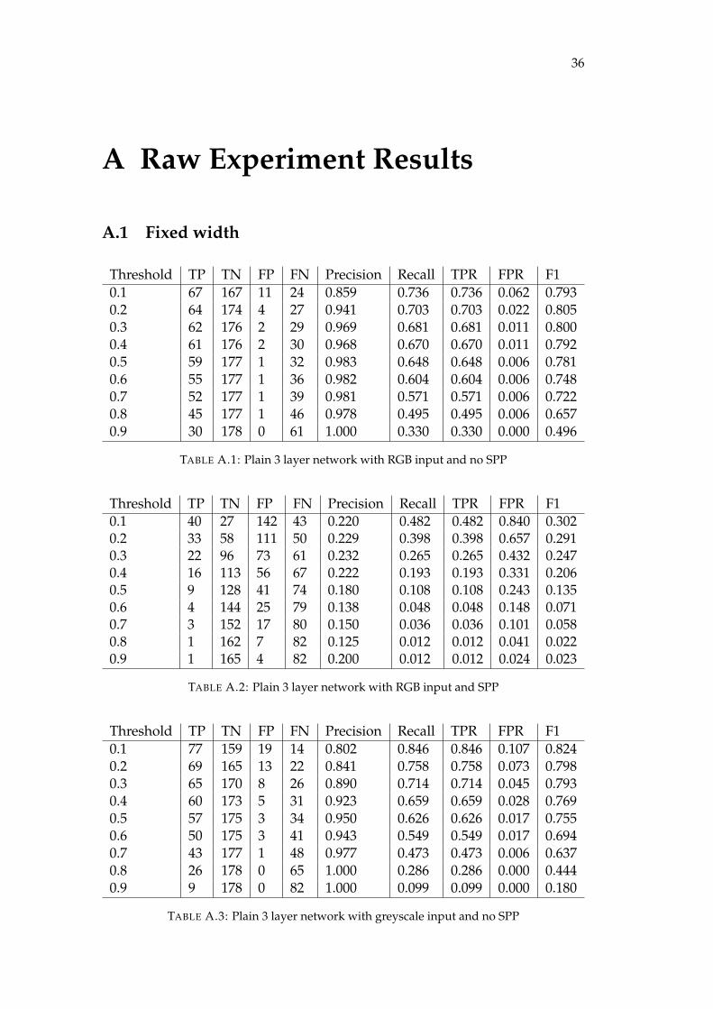
36

A Raw Experiment Results

A.1 Fixed width

Threshold TP TN FP FN Precision Recall TPR FPR F10.1 67 167 11 24 0.859 0.736 0.736 0.062 0.7930.2 64 174 4 27 0.941 0.703 0.703 0.022 0.8050.3 62 176 2 29 0.969 0.681 0.681 0.011 0.8000.4 61 176 2 30 0.968 0.670 0.670 0.011 0.7920.5 59 177 1 32 0.983 0.648 0.648 0.006 0.7810.6 55 177 1 36 0.982 0.604 0.604 0.006 0.7480.7 52 177 1 39 0.981 0.571 0.571 0.006 0.7220.8 45 177 1 46 0.978 0.495 0.495 0.006 0.6570.9 30 178 0 61 1.000 0.330 0.330 0.000 0.496

TABLE A.1: Plain 3 layer network with RGB input and no SPP

Threshold TP TN FP FN Precision Recall TPR FPR F10.1 40 27 142 43 0.220 0.482 0.482 0.840 0.3020.2 33 58 111 50 0.229 0.398 0.398 0.657 0.2910.3 22 96 73 61 0.232 0.265 0.265 0.432 0.2470.4 16 113 56 67 0.222 0.193 0.193 0.331 0.2060.5 9 128 41 74 0.180 0.108 0.108 0.243 0.1350.6 4 144 25 79 0.138 0.048 0.048 0.148 0.0710.7 3 152 17 80 0.150 0.036 0.036 0.101 0.0580.8 1 162 7 82 0.125 0.012 0.012 0.041 0.0220.9 1 165 4 82 0.200 0.012 0.012 0.024 0.023

TABLE A.2: Plain 3 layer network with RGB input and SPP

Threshold TP TN FP FN Precision Recall TPR FPR F10.1 77 159 19 14 0.802 0.846 0.846 0.107 0.8240.2 69 165 13 22 0.841 0.758 0.758 0.073 0.7980.3 65 170 8 26 0.890 0.714 0.714 0.045 0.7930.4 60 173 5 31 0.923 0.659 0.659 0.028 0.7690.5 57 175 3 34 0.950 0.626 0.626 0.017 0.7550.6 50 175 3 41 0.943 0.549 0.549 0.017 0.6940.7 43 177 1 48 0.977 0.473 0.473 0.006 0.6370.8 26 178 0 65 1.000 0.286 0.286 0.000 0.4440.9 9 178 0 82 1.000 0.099 0.099 0.000 0.180

TABLE A.3: Plain 3 layer network with greyscale input and no SPP

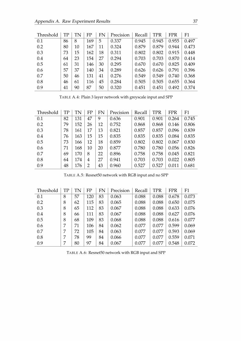
Appendix A. Raw Experiment Results 37

Threshold TP TN FP FN Precision Recall TPR FPR F10.1 86 8 169 5 0.337 0.945 0.945 0.955 0.4970.2 80 10 167 11 0.324 0.879 0.879 0.944 0.4730.3 73 15 162 18 0.311 0.802 0.802 0.915 0.4480.4 64 23 154 27 0.294 0.703 0.703 0.870 0.4140.5 61 31 146 30 0.295 0.670 0.670 0.825 0.4090.6 57 37 140 34 0.289 0.626 0.626 0.791 0.3960.7 50 46 131 41 0.276 0.549 0.549 0.740 0.3680.8 46 61 116 45 0.284 0.505 0.505 0.655 0.3640.9 41 90 87 50 0.320 0.451 0.451 0.492 0.374

TABLE A.4: Plain 3 layer network with greyscale input and SPP

Threshold TP TN FP FN Precision Recall TPR FPR F10.1 82 131 47 9 0.636 0.901 0.901 0.264 0.7450.2 79 152 26 12 0.752 0.868 0.868 0.146 0.8060.3 78 161 17 13 0.821 0.857 0.857 0.096 0.8390.4 76 163 15 15 0.835 0.835 0.835 0.084 0.8350.5 73 166 12 18 0.859 0.802 0.802 0.067 0.8300.6 71 168 10 20 0.877 0.780 0.780 0.056 0.8260.7 69 170 8 22 0.896 0.758 0.758 0.045 0.8210.8 64 174 4 27 0.941 0.703 0.703 0.022 0.8050.9 48 176 2 43 0.960 0.527 0.527 0.011 0.681

TABLE A.5: Resnet50 network with RGB input and no SPP

Threshold TP TN FP FN Precision Recall TPR FPR F10.1 8 57 120 83 0.063 0.088 0.088 0.678 0.0730.2 8 62 115 83 0.065 0.088 0.088 0.650 0.0750.3 8 65 112 83 0.067 0.088 0.088 0.633 0.0760.4 8 66 111 83 0.067 0.088 0.088 0.627 0.0760.5 8 68 109 83 0.068 0.088 0.088 0.616 0.0770.6 7 71 106 84 0.062 0.077 0.077 0.599 0.0690.7 7 72 105 84 0.063 0.077 0.077 0.593 0.0690.8 7 78 99 84 0.066 0.077 0.077 0.559 0.0710.9 7 80 97 84 0.067 0.077 0.077 0.548 0.072

TABLE A.6: Resnet50 network with RGB input and SPP

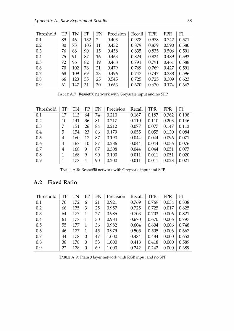
Appendix A. Raw Experiment Results 38

Threshold TP TN FP FN Precision Recall TPR FPR F10.1 89 46 132 2 0.403 0.978 0.978 0.742 0.5710.2 80 73 105 11 0.432 0.879 0.879 0.590 0.5800.3 76 88 90 15 0.458 0.835 0.835 0.506 0.5910.4 75 91 87 16 0.463 0.824 0.824 0.489 0.5930.5 72 96 82 19 0.468 0.791 0.791 0.461 0.5880.6 70 102 76 21 0.479 0.769 0.769 0.427 0.5910.7 68 109 69 23 0.496 0.747 0.747 0.388 0.5960.8 66 123 55 25 0.545 0.725 0.725 0.309 0.6230.9 61 147 31 30 0.663 0.670 0.670 0.174 0.667

TABLE A.7: Resnet50 network with Greyscale input and no SPP

Threshold TP TN FP FN Precision Recall TPR FPR F10.1 17 113 64 74 0.210 0.187 0.187 0.362 0.1980.2 10 141 36 81 0.217 0.110 0.110 0.203 0.1460.3 7 151 26 84 0.212 0.077 0.077 0.147 0.1130.4 5 154 23 86 0.179 0.055 0.055 0.130 0.0840.5 4 160 17 87 0.190 0.044 0.044 0.096 0.0710.6 4 167 10 87 0.286 0.044 0.044 0.056 0.0760.7 4 168 9 87 0.308 0.044 0.044 0.051 0.0770.8 1 168 9 90 0.100 0.011 0.011 0.051 0.0200.9 1 173 4 90 0.200 0.011 0.011 0.023 0.021

TABLE A.8: Resnet50 network with Greyscale input and SPP

A.2 Fixed Ratio

Threshold TP TN FP FN Precision Recall TPR FPR F10.1 70 172 6 21 0.921 0.769 0.769 0.034 0.8380.2 66 175 3 25 0.957 0.725 0.725 0.017 0.8250.3 64 177 1 27 0.985 0.703 0.703 0.006 0.8210.4 61 177 1 30 0.984 0.670 0.670 0.006 0.7970.5 55 177 1 36 0.982 0.604 0.604 0.006 0.7480.6 46 177 1 45 0.979 0.505 0.505 0.006 0.6670.7 44 178 0 47 1.000 0.484 0.484 0.000 0.6520.8 38 178 0 53 1.000 0.418 0.418 0.000 0.5890.9 22 178 0 69 1.000 0.242 0.242 0.000 0.389

TABLE A.9: Plain 3 layer network with RGB input and no SPP

Appendix A. Raw Experiment Results 39

Threshold TP TN FP FN Precision Recall TPR FPR F10.1 78 10 167 13 0.318 0.857 0.857 0.944 0.4640.2 61 26 151 30 0.288 0.670 0.670 0.853 0.4030.3 54 39 138 37 0.281 0.593 0.593 0.780 0.3820.4 43 58 119 48 0.265 0.473 0.473 0.672 0.3400.5 35 77 100 56 0.259 0.385 0.385 0.565 0.3100.6 25 93 84 66 0.229 0.275 0.275 0.475 0.2500.7 19 122 55 72 0.257 0.209 0.209 0.311 0.2300.8 11 144 33 80 0.250 0.121 0.121 0.186 0.1630.9 8 164 13 83 0.381 0.088 0.088 0.073 0.143

TABLE A.10: Plain 3 layer network with RGB input and SPP

Threshold TP TN FP FN Precision Recall TPR FPR F10.1 65 175 3 26 0.956 0.714 0.714 0.017 0.8180.2 56 176 2 35 0.966 0.615 0.615 0.011 0.7520.3 48 176 2 43 0.960 0.527 0.527 0.011 0.6810.4 39 177 1 52 0.975 0.429 0.429 0.006 0.5950.5 30 177 1 61 0.968 0.330 0.330 0.006 0.4920.6 21 177 1 70 0.955 0.231 0.231 0.006 0.3720.7 15 178 0 76 1.000 0.165 0.165 0.000 0.2830.8 9 178 0 82 1.000 0.099 0.099 0.000 0.1800.9 7 178 0 84 1.000 0.077 0.077 0.000 0.143

TABLE A.11: Plain 3 layer network with greyscale input and no SPP

Threshold TP TN FP FN Precision Recall TPR FPR F10.1 79 7 170 12 0.317 0.868 0.868 0.960 0.4650.2 73 11 166 18 0.305 0.802 0.802 0.938 0.4420.3 64 13 164 27 0.281 0.703 0.703 0.927 0.4010.4 61 17 160 30 0.276 0.670 0.670 0.904 0.3910.5 53 21 156 38 0.254 0.582 0.582 0.881 0.3530.6 42 30 147 49 0.222 0.462 0.462 0.831 0.3000.7 34 41 136 57 0.200 0.374 0.374 0.768 0.2610.8 26 46 131 65 0.166 0.286 0.286 0.740 0.2100.9 16 66 111 75 0.126 0.176 0.176 0.627 0.147

TABLE A.12: Plain 3 layer network with greyscale input and SPP

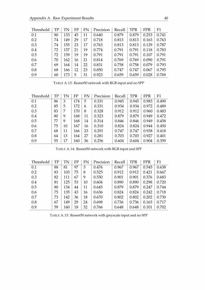
Appendix A. Raw Experiment Results 40

Threshold TP TN FP FN Precision Recall TPR FPR F10.1 80 133 45 11 0.640 0.879 0.879 0.253 0.7410.2 74 149 29 17 0.718 0.813 0.813 0.163 0.7630.3 74 155 23 17 0.763 0.813 0.813 0.129 0.7870.4 72 157 21 19 0.774 0.791 0.791 0.118 0.7830.5 72 159 19 19 0.791 0.791 0.791 0.107 0.7910.6 70 162 16 21 0.814 0.769 0.769 0.090 0.7910.7 69 164 14 22 0.831 0.758 0.758 0.079 0.7930.8 68 166 12 23 0.850 0.747 0.747 0.067 0.7950.9 60 173 5 31 0.923 0.659 0.659 0.028 0.769

TABLE A.13: Resnet50 network with RGB input and no SPP

Threshold TP TN FP FN Precision Recall TPR FPR F10.1 86 3 174 5 0.331 0.945 0.945 0.983 0.4900.2 85 5 172 6 0.331 0.934 0.934 0.972 0.4890.3 83 7 170 8 0.328 0.912 0.912 0.960 0.4830.4 80 9 168 11 0.323 0.879 0.879 0.949 0.4720.5 77 9 168 14 0.314 0.846 0.846 0.949 0.4580.6 75 10 167 16 0.310 0.824 0.824 0.944 0.4500.7 68 11 166 23 0.291 0.747 0.747 0.938 0.4180.8 64 13 164 27 0.281 0.703 0.703 0.927 0.4010.9 55 17 160 36 0.256 0.604 0.604 0.904 0.359

TABLE A.14: Resnet50 network with RGB input and SPP

Threshold TP TN FP FN Precision Recall TPR FPR F10.1 88 81 97 3 0.476 0.967 0.967 0.545 0.6380.2 83 103 75 8 0.525 0.912 0.912 0.421 0.6670.3 82 111 67 9 0.550 0.901 0.901 0.376 0.6830.4 81 125 53 10 0.604 0.890 0.890 0.298 0.7200.5 80 134 44 11 0.645 0.879 0.879 0.247 0.7440.6 75 135 43 16 0.636 0.824 0.824 0.242 0.7180.7 73 142 36 18 0.670 0.802 0.802 0.202 0.7300.8 67 149 29 24 0.698 0.736 0.736 0.163 0.7170.9 59 160 18 32 0.766 0.648 0.648 0.101 0.702

TABLE A.15: Resnet50 network with greyscale input and no SPP

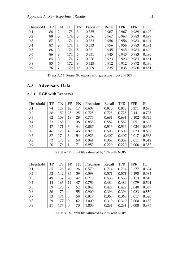
Appendix A. Raw Experiment Results 41

Threshold TP TN FP FN Precision Recall TPR FPR F10.1 88 2 175 3 0.335 0.967 0.967 0.989 0.4970.2 88 3 174 3 0.336 0.967 0.967 0.983 0.4990.3 87 3 174 4 0.333 0.956 0.956 0.983 0.4940.4 87 3 174 4 0.333 0.956 0.956 0.983 0.4940.5 86 3 174 5 0.331 0.945 0.945 0.983 0.4900.6 86 3 174 5 0.331 0.945 0.945 0.983 0.4900.7 84 3 174 7 0.326 0.923 0.923 0.983 0.4810.8 83 5 172 8 0.325 0.912 0.912 0.972 0.4800.9 76 7 170 15 0.309 0.835 0.835 0.960 0.451

TABLE A.16: Resnet50 network with greyscale input and SPP

A.3 Adversary Data

A.3.1 RGB with Resnet50

Threshold TP TN FP FN Precision Recall TPR FPR F10.1 74 129 48 17 0.607 0.813 0.813 0.271 0.6950.2 66 152 25 25 0.725 0.725 0.725 0.141 0.7250.3 62 159 18 29 0.775 0.681 0.681 0.102 0.7250.4 53 168 9 38 0.855 0.582 0.582 0.051 0.6930.5 47 171 6 44 0.887 0.516 0.516 0.034 0.6530.6 46 173 4 45 0.920 0.505 0.505 0.023 0.6520.7 37 174 3 54 0.925 0.407 0.407 0.017 0.5650.8 32 175 2 59 0.941 0.352 0.352 0.011 0.5120.9 20 176 1 71 0.952 0.220 0.220 0.006 0.357

TABLE A.17: Input file saturated by 10% with NOPs

Threshold TP TN FP FN Precision Recall TPR FPR F10.1 65 128 49 26 0.570 0.714 0.714 0.277 0.6340.2 52 142 35 39 0.598 0.571 0.571 0.198 0.5840.3 49 157 20 42 0.710 0.538 0.538 0.113 0.6130.4 44 163 14 47 0.759 0.484 0.484 0.079 0.5910.5 39 170 7 52 0.848 0.429 0.429 0.040 0.5690.6 36 173 4 55 0.900 0.396 0.396 0.023 0.5500.7 33 174 3 58 0.917 0.363 0.363 0.017 0.5200.8 29 177 0 62 1.000 0.319 0.319 0.000 0.4830.9 21 177 0 70 1.000 0.231 0.231 0.000 0.375

TABLE A.18: Input file saturated by 20% with NOPs

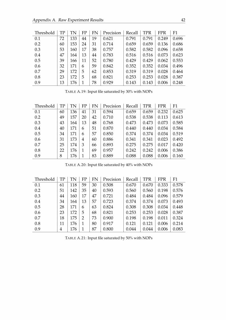
Appendix A. Raw Experiment Results 42

Threshold TP TN FP FN Precision Recall TPR FPR F10.1 72 133 44 19 0.621 0.791 0.791 0.249 0.6960.2 60 153 24 31 0.714 0.659 0.659 0.136 0.6860.3 53 160 17 38 0.757 0.582 0.582 0.096 0.6580.4 47 164 13 44 0.783 0.516 0.516 0.073 0.6230.5 39 166 11 52 0.780 0.429 0.429 0.062 0.5530.6 32 171 6 59 0.842 0.352 0.352 0.034 0.4960.7 29 172 5 62 0.853 0.319 0.319 0.028 0.4640.8 23 172 5 68 0.821 0.253 0.253 0.028 0.3870.9 13 176 1 78 0.929 0.143 0.143 0.006 0.248

TABLE A.19: Input file saturated by 30% with NOPs

Threshold TP TN FP FN Precision Recall TPR FPR F10.1 60 136 41 31 0.594 0.659 0.659 0.232 0.6250.2 49 157 20 42 0.710 0.538 0.538 0.113 0.6130.3 43 164 13 48 0.768 0.473 0.473 0.073 0.5850.4 40 171 6 51 0.870 0.440 0.440 0.034 0.5840.5 34 171 6 57 0.850 0.374 0.374 0.034 0.5190.6 31 173 4 60 0.886 0.341 0.341 0.023 0.4920.7 25 174 3 66 0.893 0.275 0.275 0.017 0.4200.8 22 176 1 69 0.957 0.242 0.242 0.006 0.3860.9 8 176 1 83 0.889 0.088 0.088 0.006 0.160

TABLE A.20: Input file saturated by 40% with NOPs

Threshold TP TN FP FN Precision Recall TPR FPR F10.1 61 118 59 30 0.508 0.670 0.670 0.333 0.5780.2 51 142 35 40 0.593 0.560 0.560 0.198 0.5760.3 44 160 17 47 0.721 0.484 0.484 0.096 0.5790.4 34 164 13 57 0.723 0.374 0.374 0.073 0.4930.5 28 171 6 63 0.824 0.308 0.308 0.034 0.4480.6 23 172 5 68 0.821 0.253 0.253 0.028 0.3870.7 18 175 2 73 0.900 0.198 0.198 0.011 0.3240.8 11 176 1 80 0.917 0.121 0.121 0.006 0.2140.9 4 176 1 87 0.800 0.044 0.044 0.006 0.083

TABLE A.21: Input file saturated by 50% with NOPs

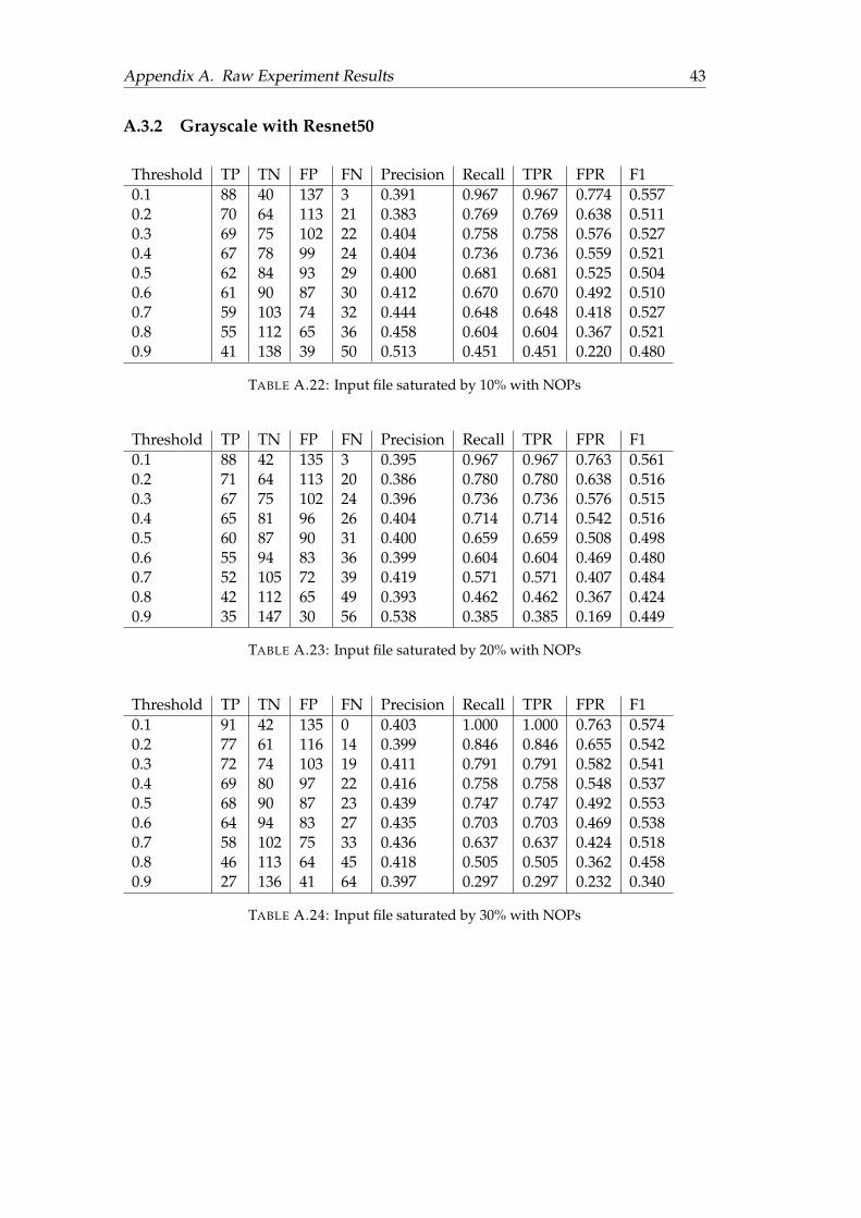
Appendix A. Raw Experiment Results 43

A.3.2 Grayscale with Resnet50

Threshold TP TN FP FN Precision Recall TPR FPR F10.1 88 40 137 3 0.391 0.967 0.967 0.774 0.5570.2 70 64 113 21 0.383 0.769 0.769 0.638 0.5110.3 69 75 102 22 0.404 0.758 0.758 0.576 0.5270.4 67 78 99 24 0.404 0.736 0.736 0.559 0.5210.5 62 84 93 29 0.400 0.681 0.681 0.525 0.5040.6 61 90 87 30 0.412 0.670 0.670 0.492 0.5100.7 59 103 74 32 0.444 0.648 0.648 0.418 0.5270.8 55 112 65 36 0.458 0.604 0.604 0.367 0.5210.9 41 138 39 50 0.513 0.451 0.451 0.220 0.480

TABLE A.22: Input file saturated by 10% with NOPs

Threshold TP TN FP FN Precision Recall TPR FPR F10.1 88 42 135 3 0.395 0.967 0.967 0.763 0.5610.2 71 64 113 20 0.386 0.780 0.780 0.638 0.5160.3 67 75 102 24 0.396 0.736 0.736 0.576 0.5150.4 65 81 96 26 0.404 0.714 0.714 0.542 0.5160.5 60 87 90 31 0.400 0.659 0.659 0.508 0.4980.6 55 94 83 36 0.399 0.604 0.604 0.469 0.4800.7 52 105 72 39 0.419 0.571 0.571 0.407 0.4840.8 42 112 65 49 0.393 0.462 0.462 0.367 0.4240.9 35 147 30 56 0.538 0.385 0.385 0.169 0.449

TABLE A.23: Input file saturated by 20% with NOPs

Threshold TP TN FP FN Precision Recall TPR FPR F10.1 91 42 135 0 0.403 1.000 1.000 0.763 0.5740.2 77 61 116 14 0.399 0.846 0.846 0.655 0.5420.3 72 74 103 19 0.411 0.791 0.791 0.582 0.5410.4 69 80 97 22 0.416 0.758 0.758 0.548 0.5370.5 68 90 87 23 0.439 0.747 0.747 0.492 0.5530.6 64 94 83 27 0.435 0.703 0.703 0.469 0.5380.7 58 102 75 33 0.436 0.637 0.637 0.424 0.5180.8 46 113 64 45 0.418 0.505 0.505 0.362 0.4580.9 27 136 41 64 0.397 0.297 0.297 0.232 0.340

TABLE A.24: Input file saturated by 30% with NOPs

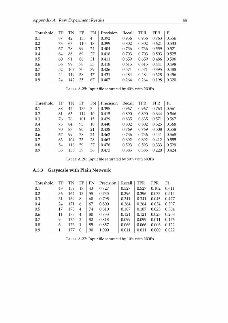
Appendix A. Raw Experiment Results 44

Threshold TP TN FP FN Precision Recall TPR FPR F10.1 87 42 135 4 0.392 0.956 0.956 0.763 0.5560.2 73 67 110 18 0.399 0.802 0.802 0.621 0.5330.3 67 78 99 24 0.404 0.736 0.736 0.559 0.5210.4 64 88 89 27 0.418 0.703 0.703 0.503 0.5250.5 60 91 86 31 0.411 0.659 0.659 0.486 0.5060.6 56 99 78 35 0.418 0.615 0.615 0.441 0.4980.7 52 107 70 39 0.426 0.571 0.571 0.395 0.4880.8 44 119 58 47 0.431 0.484 0.484 0.328 0.4560.9 24 142 35 67 0.407 0.264 0.264 0.198 0.320

TABLE A.25: Input file saturated by 40% with NOPs

Threshold TP TN FP FN Precision Recall TPR FPR F10.1 88 42 135 3 0.395 0.967 0.967 0.763 0.5610.2 81 63 114 10 0.415 0.890 0.890 0.644 0.5660.3 76 76 101 15 0.429 0.835 0.835 0.571 0.5670.4 73 84 93 18 0.440 0.802 0.802 0.525 0.5680.5 70 87 90 21 0.438 0.769 0.769 0.508 0.5580.6 67 99 78 24 0.462 0.736 0.736 0.441 0.5680.7 63 104 73 28 0.463 0.692 0.692 0.412 0.5550.8 54 118 59 37 0.478 0.593 0.593 0.333 0.5290.9 35 138 39 56 0.473 0.385 0.385 0.220 0.424

TABLE A.26: Input file saturated by 50% with NOPs

A.3.3 Grayscale with Plain Network

Threshold TP TN FP FN Precision Recall TPR FPR F10.1 48 159 18 43 0.727 0.527 0.527 0.102 0.6110.2 36 164 13 55 0.735 0.396 0.396 0.073 0.5140.3 31 169 8 60 0.795 0.341 0.341 0.045 0.4770.4 24 171 6 67 0.800 0.264 0.264 0.034 0.3970.5 17 173 4 74 0.810 0.187 0.187 0.023 0.3040.6 11 173 4 80 0.733 0.121 0.121 0.023 0.2080.7 9 175 2 82 0.818 0.099 0.099 0.011 0.1760.8 6 176 1 85 0.857 0.066 0.066 0.006 0.1220.9 1 177 0 90 1.000 0.011 0.011 0.000 0.022

TABLE A.27: Input file saturated by 10% with NOPs

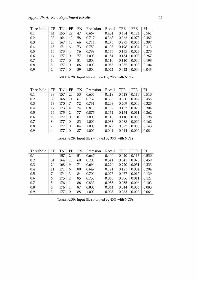
Appendix A. Raw Experiment Results 45

Threshold TP TN FP FN Precision Recall TPR FPR F10.1 44 155 22 47 0.667 0.484 0.484 0.124 0.5610.2 33 164 13 58 0.717 0.363 0.363 0.073 0.4820.3 25 167 10 66 0.714 0.275 0.275 0.056 0.3970.4 18 171 6 73 0.750 0.198 0.198 0.034 0.3130.5 15 173 4 76 0.789 0.165 0.165 0.023 0.2730.6 14 177 0 77 1.000 0.154 0.154 0.000 0.2670.7 10 177 0 81 1.000 0.110 0.110 0.000 0.1980.8 5 177 0 86 1.000 0.055 0.055 0.000 0.1040.9 2 177 0 89 1.000 0.022 0.022 0.000 0.043

TABLE A.28: Input file saturated by 20% with NOPs

Threshold TP TN FP FN Precision Recall TPR FPR F10.1 38 157 20 53 0.655 0.418 0.418 0.113 0.5100.2 30 166 11 61 0.732 0.330 0.330 0.062 0.4550.3 19 170 7 72 0.731 0.209 0.209 0.040 0.3250.4 17 173 4 74 0.810 0.187 0.187 0.023 0.3040.5 14 175 2 77 0.875 0.154 0.154 0.011 0.2620.6 10 177 0 81 1.000 0.110 0.110 0.000 0.1980.7 8 177 0 83 1.000 0.088 0.088 0.000 0.1620.8 7 177 0 84 1.000 0.077 0.077 0.000 0.1430.9 4 177 0 87 1.000 0.044 0.044 0.000 0.084

TABLE A.29: Input file saturated by 30% with NOPs

Threshold TP TN FP FN Precision Recall TPR FPR F10.1 40 157 20 51 0.667 0.440 0.440 0.113 0.5300.2 31 164 13 60 0.705 0.341 0.341 0.073 0.4590.3 20 168 9 71 0.690 0.220 0.220 0.051 0.3330.4 11 171 6 80 0.647 0.121 0.121 0.034 0.2040.5 7 174 3 84 0.700 0.077 0.077 0.017 0.1390.6 6 175 2 85 0.750 0.066 0.066 0.011 0.1210.7 5 176 1 86 0.833 0.055 0.055 0.006 0.1030.8 4 176 1 87 0.800 0.044 0.044 0.006 0.0830.9 3 177 0 88 1.000 0.033 0.033 0.000 0.064

TABLE A.30: Input file saturated by 40% with NOPs

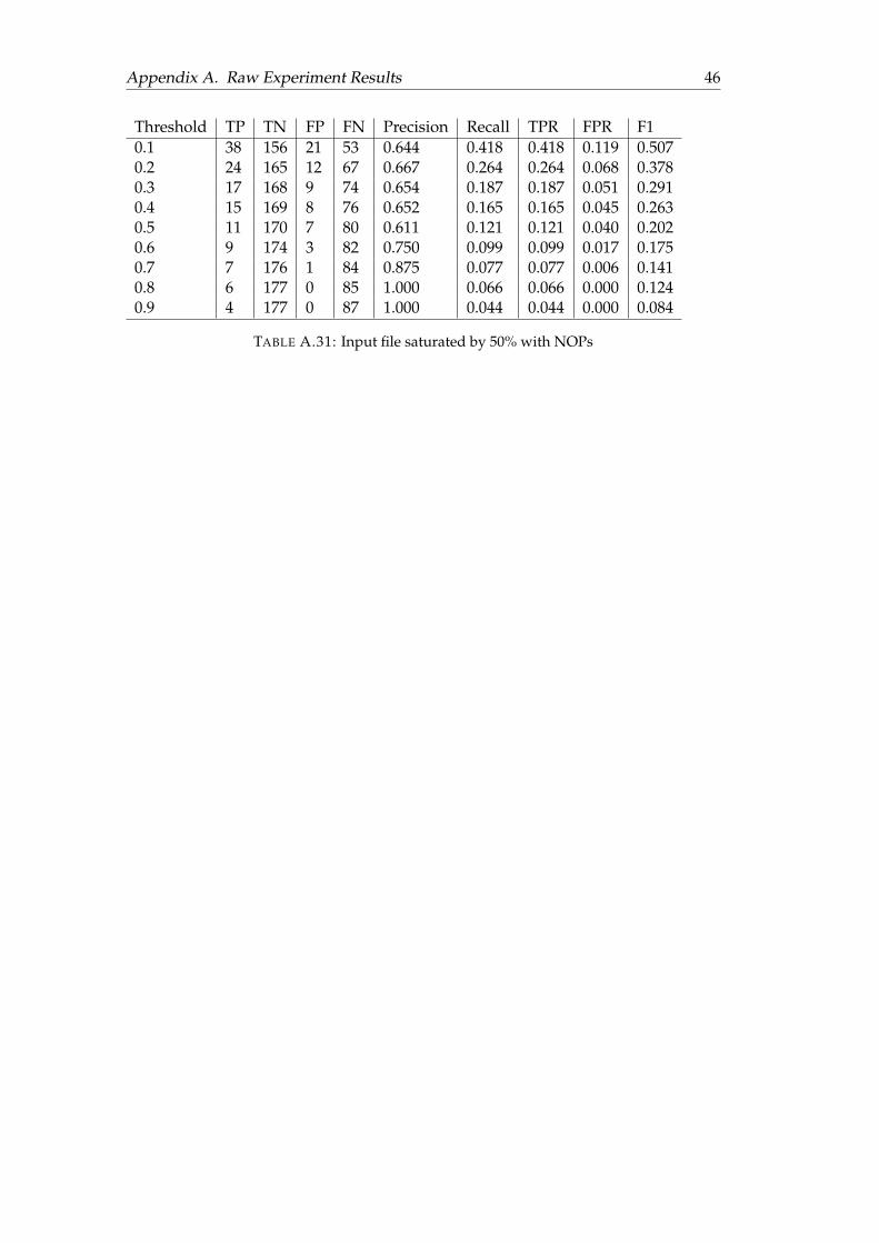
Appendix A. Raw Experiment Results 46

Threshold TP TN FP FN Precision Recall TPR FPR F10.1 38 156 21 53 0.644 0.418 0.418 0.119 0.5070.2 24 165 12 67 0.667 0.264 0.264 0.068 0.3780.3 17 168 9 74 0.654 0.187 0.187 0.051 0.2910.4 15 169 8 76 0.652 0.165 0.165 0.045 0.2630.5 11 170 7 80 0.611 0.121 0.121 0.040 0.2020.6 9 174 3 82 0.750 0.099 0.099 0.017 0.1750.7 7 176 1 84 0.875 0.077 0.077 0.006 0.1410.8 6 177 0 85 1.000 0.066 0.066 0.000 0.1240.9 4 177 0 87 1.000 0.044 0.044 0.000 0.084

TABLE A.31: Input file saturated by 50% with NOPs