Making Work Pay in Nicaragua: Employment, Growth, and Poverty Reduction (Directions in Development)
146
DIRECTIONS IN DEVELOPMENT Poverty Making Work Pay in Nicaragua Employment, Growth, and Poverty Reduction Catalina Gutierrez, Pierella Paci, and Marco Ranzani
-
Upload
catalina-gutierrez -
Category
Documents
-
view
212 -
download
0
Transcript of Making Work Pay in Nicaragua: Employment, Growth, and Poverty Reduction (Directions in Development)

D I R E C T I O N S I N D E V E L O P M E N T
Poverty
Making Work Pay in NicaraguaEmployment, Growth, and Poverty Reduction
Catalina Gutierrez, Pierella Paci, and Marco Ranzani
Poor people derive most of their income from work. However, there is insufficient under-standing of the role of employment and earnings as a link between growth and povertyreduction, especially in low-income countries. The Making Work Pay series analyzes theimportant roles of labor markets, employment, productivity, and labor income in facilitatingshared growth and promoting poverty reduction.
Making Work Pay in Nicaragua provides a description of the trends in growth, poverty andlabor market outcomes in Nicaragua. It assesses the linkages among changes in output,employment, and labor productivity and links changes in the quality and quantity ofemployment to poverty reduction. The book also addresses other key issues such as ruralversus urban conditions, women and children in the labor market, self-employment andhousehold enterprises, and it identifies priorities for further analysis and policy intervention.
Making Work Pay in Nicaragua will be of interest to development practitioners in interna-tional organizations, governments, research institutions, and universities with an interestin inclusive growth and the creation of productive employment.
ISBN 978-0-8213-7534-1
SKU 17534

Making Work Pay in Nicaragua


Making Work Pay in Nicaragua Employment, Growth, and Poverty ReductionCatalina GutierrezPierella PaciMarco Ranzani

© 2008 The International Bank for Reconstruction and Development/ The World Bank1818 H Street NWWashington DC 20433Telephone: 202-473-1000Internet: www.worldbank.orgE-mail: [email protected]
All rights reserved.
1 2 3 4 11 10 09 08
This volume is a product of the staff of the International Bank for Reconstructionand Development/The World Bank. The findings, interpretations, and conclusionsexpressed in this volume do not necessarily reflect the views of the ExecutiveDirectors of The World Bank or the governments they represent.
The World Bank does not guarantee the accuracy of the data included in thiswork. The boundaries, colors, denominations, and other information shown on anymap in this work do not imply any judgment on the part of The World Bank con-cerning the legal status of any territory or the endorsement or acceptance of suchboundaries.
Rights and PermissionsThe material in this publication is copyrighted. Copying and/or transmitting por-tions or all of this work without permission may be a violation of applicable law. TheInternational Bank for Reconstruction and Development / The World Bank encour-ages dissemination of its work and will normally grant permission to reproduce por-tions of the work promptly.
For permission to photocopy or reprint any part of this work, please send arequest with complete information to the Copyright Clearance Center Inc., 222Rosewood Drive, Danvers, MA 01923, USA; telephone: 978-750-8400; fax: 978-750-4470; Internet: www.copyright.com.
All other queries on rights and licenses, including subsidiary rights, should beaddressed to the Office of the Publisher, The World Bank, 1818 H Street NW,Washington, DC 20433, USA; fax: 202-522-2422; e-mail: [email protected].
ISBN-13: 978-0-8213-7534-2eISBN: 978-0-8213-7535-8DOI: 10.1596/978-0-8213-7534-1
Library of Congress Cataloging-in-Publication Data
Making work pay in Nicaragua: employment, growth, and poverty reduction /edited by Catalina Gutiérrez, Pierella Paci, Marco Ranzani.
p. cm.Includes bibliographical references and index.ISBN 978-0-8213-7534-1 -- ISBN 978-0-8213-7535-8 (electronic)
1. Labor market--Nicaragua. 2. Wages--Nicaragua. 3. Poverty--Nicaragua. 4. Laborproductivity--Nicaragua. I. Gutiérrez, Catalina. II. Paci, Pierella, 1957- III. Ranzani,Marco, 1979- HD5737.A6M34 2008331.1097285--dc22
2008017702
Cover design: Candace Roberts, Quantum Think, Philadelphia, PA, United States

Acronyms and Abbreviations xiAcknowledgments xiii
Chapter 1 Introduction and Overview 1Objectives and Scope of this Task 2Structure of the Report 3
Chapter 2 Country Context 7Macroeconomic Context 7Labor Market Context 10Labor Regulation in Nicaragua 20
Chapter 3 Output, Population, Employment, and Poverty 27Main Trends in Output 27Main Trends in Population 28Main Trends in Employment 30Main Trends in Poverty 31Decomposition of Per Capita Income Growth 32
Contents
v
A Closer Look at the Manufacturing Sector 42Annex 3A. Decomposition of Per Capita 48
Value Added Growth
Chapter 4 Employment and Labor Income Profile 59of the PopulationIncome and Employment Profile 60Decomposition of Changes in Labor Income 63A Closer Look at Agriculture 69Annex 4A. Decomposition of Labor Income 78
GrowthAnnex 4B. Estimation Results 81
Chapter 5 Segmentation and Skill Mismatch 87Labor Market Segmentation: Basic Assumptions
and Literature Review 87Evidence of Segmentation across Different
Dimensions 90Segmentation and Barriers to Mobility:
A Qualitative Approach 103Skill Mismatch 107
Chapter 6 Policy Implications and Further Research 115
References 119Index 125
Figures2.1 Investment, Exports, and Growth, 1995–2005 92.2 Distribution of Wages by Sector and Formality, 2001 243.1 Change in Population Structure, 2001–05 293.2 Share of Employment by Sectors, 2001 and 2005 313.3 Aggregate Employment and Productivity Profile of 35
Growth, 2001–053.4 Decomposition of Changes in Output per Worker, 37
2001–054.1 Growth in Average Per Capita Income, by Quintile, 2001 684.2 Productivity of Sensitive Products by Yield per Hectare, 71
1990–2005
vi Contents
4.3 Relative Productivity by Product, 1990–2005 724.4 Area Harvested for Sensitive Products, 1990–2005 734.5 Production Volume for Sensitive Products, 1990–2005 744.6 Producer Prices Relative to Consumer Prices for 75
Export Goods, 1999–20064.7 Relative Prices of Trade for Meat, 1999–2006 754.8 Relative Prices for Cereals, 1999–2006 764.9 Relative Prices for Sensitive Products, 2001–06 765.1 Hourly Earnings by Employment Category, 2001 935.2 Hourly Earnings by Broad Sector and Informality, 2001 945.3 Changes in the Skill Premium and the Relative Supply 109
of Skills, of Total Wage Workers, 2001–055.4 Changes in the Skill Premium and the Relative Supply 110
of Skills, of Urban Wage Workers, 2001–05
Tables2.1 Main Macroeconomic Indicators, 1998–2005 112.2 Main Indicators of the Labor Market, 2001 and 2005 132.3 Earnings and Income by Employment Category, 14
2001 and 20052.4 Hierarchical Description of the Population Six Years 16
of Age and Above, 2001 and 20052.5 Other Characteristics of the Employed, 2001 and 2005 182.6 Labor Market Flexibility, Comparative Performance 212.7 Issues Affecting the Investment Climate 222.8 Minimum Wage and Lowest Wage Paid as a Proportion 23
of Minimum Wage, 2001 and 20053.1 Sectoral Growth, 1998–2005 283.2 Average Level of Education of Population Ages 25 to 64 303.3 Evolution of Employment by Sectors, 2001 and 2005 323.4 Headcount Poverty Rates of the Working-Age Population 33
by Employment Status, 2001–053.5 Employment by Sector and Poverty Level, Shares of 34
Total Employment, 2001 and 20053.6 Percentage Change in Selected Variables, 2001–05 353.7 Decomposition of Intersectoral Shifts 393.8 Sectoral Growth, 2001–05 39
Contents vii
3.9 Employment Shares and Productivity, by Sectors of 40Economic Activity, 2001–05
3.10 Total Sectoral Contribution to Growth, 2001–05 413.11 Wages by Sector of Economic Activity, 2001 and 2005 423.12 Employment Generation by Subsector, 2001 and 2005 433.13 Wages in the Manufacturing Sector, 2001 and 2005 443.14 Employment Generation in Manufacturing by Type 44
of Employment, 2001 and 20054.1 Employment Status of the Working-Age Population 61
by Quintile, 2001 and 20054.2 Employment Status of the Working-Age Population by 61
Poverty Level, 2001 and 20054.3 Employment Categories by Quintile, 2001 and 2005 624.4 Employment Categories by Poverty Level, 2001 and 2005 624.5 Structure of Income by Quintile, 2001 and 2005 644.6 Structure of Income by Poverty Level, 2001 and 2005 644.7 Labor Profile of the Population by Poverty Level,
2001 and 2005 654.8 Labor Profile of the Population by Quintile, 67
2001 and 20054.9 Per Capita Household Income Changes, by Quintile, 68
2001–054.10 Shapley Decomposition of Per Capita Labor Income, 70
by Quintile4.11 Number of Farms, by Sensitive Product, according to 71
Farm Size, 20014B.1 Mean and Standard Deviation, by Employment 81
Category4B.2 Mean and Standard Deviation, by Sector of Economic 82
Activity and Formality Level4B.3 Earnings Equations by Employment Category, 2001 834B.4 Earnings Equations by Sector of Employment, 2001 844B.5 Oaxaca-Blinder Decomposition: Detailed Outcomes 85
for Sector and Informality4B.6 Oaxaca-Blinder Decomposition: Detailed Outcomes 86
for Employment Categories
viii Contents
5.1 Selection among Employment Categories, 2001 975.2 Selection among Sectors, 2001 985.3 Oaxaca-Blinder Decomposition by Employment 100
Category5.4 Oaxaca-Blinder Decomposition by Employment Sector 1015.5 Reason for Starting a Business, by Level of Education, 104
20015.6 Reason for Starting a Business, by Poverty Level, 2001 1055.7 Skills and Education of Available Workers as an 112
Obstacle to Firms’ Operation and Growth, 2003
Boxes1.1 Definitions 42.1 Urban versus Rural Population: Possible Data Problems 193.1 Evolution of the Maquila Sector and Its Importance in 45
the Employment Growth in Manufacturing
Contents ix


BCN Central Bank of NicaraguaCAFTA Central American Free Trade Agreement CEPAL Economic Commission for Latin America and
the CaribbeanCPI consumer price indexEMNV National Household Living Standards Survey
(Encuesta de Medición del Nivel de Vida) EPZ export processing zoneFAO Food and Agriculture Organization of the United NationsGDP gross domestic productHIPC heavily indebted poor countriesIFC International Finance CorporationILO International Labour OrganizationIMF International Monetary FundINATEC National Technology Institute
(Instituto Nacional Tecnológico)INEC National Institute of Statistics and Census
(Instituto National de Estadísticas y Censos)
Acronyms and Abbreviations
xi

xii Acronyms and Abbreviations
INIDE National Institute for Development InformationMITRAB Ministry of Labor PRGF Poverty Reduction and Growth FacilityRAAS Autonomous Region of the Atlantic South
(Región Autónoma del Atlántico Sur)RRR relative risk ratio

This report was prepared by Catalina Gutierrez, Pierella Paci and MarcoRanzani in the Jobs and Migration cluster in the Poverty Reduction andDevelopment Effectiveness Group at the World Bank as part of a multi-year program on the role of employment for inclusive growth. It also pro-vided background information for the Poverty Assessment of Nicaraguaproduced by the World Bank.
The team would like to thank very much a number of people withoutwhom this report would not have been possible. First, the Minister ofLabor of Nicaragua, Janeth Chavéz Gómez, for taking time to provide uswith detailed explanations of the characteristics and peculiarities of theNicaraguan labor market and for sharing with us her view on priorityissues. Second, the staff of the Central Bank of Nicaragua, who havealways responded positively to our many data and information requests.The team is particularly indebted to the Director of the ResearchDepartment, Mario Alemán, and, among his staff, Hiparco Loaisiga, JesusRojas, Ligia Miranda, Miguel Aguilar, and Lisbeth Laguna, who sharedtheir knowledge and views with us in addition to providing us withinvaluable data and information. The team is also grateful to Juan Rocha
Acknowledgments
xiii
xiv Acknowledgments
of the Statistical and Census Office in Nicaragua for his help with house-hold surveys and to Alejandro Martinéz Cuenca in FundaciónInternacional para el Desafío Económico Global (FIDEG), who was kindenough to share his views on the challenges faced by the Nicaraguaneconomy. Finally, special thanks go to Nydia Betanco in the NicaraguaWorld Bank Country Office for all her help and support while on missionin Nicaragua.
The report benefited greatly from the comments received from themembers of the Nicaragua Poverty Assessment Team, led by FlorenciaCastro-Leal, and from the participants to the seminar held in Managua,March 16–17, 2007. We are particularly grateful to Florencia, NormanHicks, Gabriel Demombynes, Diego Angel-Urdinola, Ximena Del Carpio,and José Ramón Laguna for helpful comments and advice. The manyinputs of the members of the Employment and Migration team in thePoverty Reduction and Debt Effectiveness Unit at the World Bank werealso invaluable. The team is extremely grateful for these inputs.

The degree to which growth is able to translate into poverty reductiondepends on how its benefits are distributed among different segments ofsociety. There is little doubt that growth—measured by changes in aver-age income—contributes significantly to poverty reduction.1 However, itis also clear that countries differ in the degree to which income growthspells have translated into poverty reduction. Although differences in theresponsiveness of poverty to income growth account for a small fractionof the overall differences in poverty changes across countries, from thepoint of view of an individual country, these differences may have signif-icant implications for poverty reduction, especially in the short term.2
There is a general consensus that the availability of employmentopportunities and their characteristics constitute an essential transmis-sion channel from growth to poverty reduction and, in this way, play akey role in poverty’s response to growth. For one thing, the poor derivemost of their income from work, either as self-employed or as employees,so what happens to their income and employment status seems tautolog-ically relevant. In addition, the ease with which the poor may take up theopportunities afforded by growth may depend crucially on (i) the struc-ture of employment, (ii) the returns to labor and their distribution, and
C H A P T E R 1
Introduction and Overview
1
(iii) the existence of imperfections and frictions in the labor markets. Forexample, one may be inclined to believe that when the poor face flexiblelabor markets and low barriers to mobility across labor market segments,geographic regions, or sectors of production, they are in a better positionto take the opportunities generated by growth, by moving more easily tothe growing sectors. Similarly, the effectiveness of growth in reducingpoverty may also depend on whether growth is unskilled labor–intensiveand whether the poor have or can easily acquire the skills required by thegrowing sectors. Moreover, there is some evidence of strong links betweenlabor market regulations, such as minimum wages, and the incidence ofpoverty in developing countries.
The concern that employment, returns to labor, and imperfections orrigidities in the labor markets play a crucial role in the poverty impact ofgrowth has been reflected in the emphasis in the policy debate on theidea that jobless growth has been responsible for the disappointing resultsseen by some countries in the effectiveness of growth in reducing pover-ty. As a result, debates addressing how to foster employment-intensivegrowth have followed.3 However, it is also often recognized that povertyis less an outcome of open unemployment than of adequate levels ofincome, and as such, emphasis should be placed not on increasingemployment levels but on increasing the productivity of the workingpoor (ILO 2003). The debate has also been concerned with whether pol-icy interventions should concentrate on increasing earnings in the sectorswhere the poor are found (such as agriculture), or whether they shouldbe targeted to sectors where the poor are not found, so that more of thepoor can be drawn into the higher-earning sectors (Fields 2006). To date,there is very little evidence to illuminate the debate. Moreover, the ques-tions are hard to address, because there is lack of clarity on how to achievethe alternative objectives and because it is inherently difficult to identifythe costs and benefits of the possible policy alternatives.
Objectives and Scope of this Task
The objective of this report is to shed light on some of the issues dis-cussed above in the case of Nicaragua, and to provide some policy guide-lines for the fight against poverty. In particular, it hopes to be able to iden-tify the growing sectors, as well as the constraints faced by the poor inbenefiting from this growth.
2 Making Work Pay in Nicaragua: Employment, Growth, and Poverty Reduction
Introduction and Overview 3
The report is part of a series of studies conducted within the PRMPRto foster understanding of the role of employment earnings and labormarkets in shared growth. In addition, it is intended to function as a back-ground document for the World Bank’s Nicaragua Poverty Assessment2007.
Structure of the Report
The report is structured in six chapters. Chapter 2 briefly describes theevolution of the Nicaraguan economy, in terms of its macroeconomicindicators, employment, and poverty. The third chapter analyzes the pro-file of growth and the way in which it helps explain the observed behav-ior of poverty, using data from national accounts and employment datafrom household surveys. It describes growth and employment by the sec-tor of economic activity and its employment productivity profile. Thechapter goes more deeply into the evolution of the manufacturing sectorand the maquila production. Chapter 4 looks at the income profile of thepopulation, using household surveys. Segmentation and skill mismatchare explored in chapter 5, and chapter 6 provides a brief statement onpolicy implications and further research.
Definitions of terms used throughout the report are presented below.Workers have been classified into four occupational categories: waged andsalaried workers, individual self-employed workers, family enterpriseworkers, and employers. These are considered qualitatively distinct typesof labor. Each might constitute a segment within the labor market, withdifferent rules for earnings determination and different employment poli-cies for individuals of identical productivity, and workers’ mobilitybetween these employment categories might be limited. The nonwageworkers are divided into the above-mentioned categories for several rea-sons. First, employers (those who employ paid labor) receive substantial-ly higher income than other nonwage workers and are better educated.They often have assets that other nonwage workers do not. Second,returns to labor for family enterprise workers and the self-employed whoare not working with other members of the family need differentmethodologies of calculation. While the income reported by the self-employed working alone is the return for labor for his or her individualwork, reported income for self-employed workers working with other

4 Making Work Pay in Nicaragua: Employment, Growth, and Poverty Reduction
Box 1.1
Definitions
Employment
Child labor A child between 6 and 14 years of age who performed market activities for at least one hour in the week prior to the survey, or who has a permanent job.
Employed An individual who performed market activities for at least one hour in the week prior to the survey, or who has a permanent job.
Formal Employment for which social security contributions are paid employment by workers and firms.
Household A self-declared self-employed person living in a household enterprise worker, with other self-employed or unpaid family workers.family enterprise worker
Inactive A person who is neither employed nor actively looking for work.
Labor force The sum of the working-age employed and unemployed.
Labor market The place where labor services are bought, sold, and exchanged. The labor market comprises wage and salaried workers and their employers, but also nonwage family enterprise workers and the self-employed, who make up the largest share of workers in Nicaragua.
Maquila sector The maquila sector comprises all production units located in the special export processing zones (EPZs), which are clearly defined zones, often within a wired complex. Produc-tion is undertaken with mostly imported materials using local labor, and all output is destined for export markets. Employment in the maquila sector is referred to as maquila employment.
Self-employed A self-declared self-employed person, living in a household in which there are no other self-employed or unpaid family workers.
Unemployed A working-age individual who is not employed but is actively looking for work.
(continued)
Introduction and Overview 5
Box 1.1
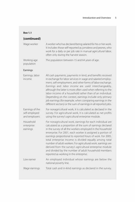
(continued)Wage worker A worker who has declared being salaried for his or her work.
It includes those self-reported as jornaleros and peones, who work for a daily or per job rate in manual agricultural labor, often only during the harvest season.
Working-age The population between 15 and 64 years of age.population
Earnings
Earnings, labor All cash payments, payments in kind, and benefits received income in exchange for labor services in wage and salaried employ-
ment, self-employment, and other forms of labor exchange. Earnings and labor income are used interchangeably, although the latter is more often used when referring to the labor income of a household rather than of an individual. Depending on the context, earnings include only primary job earnings (for example, when comparing earnings in the different sectors) or the sum of earnings in all reported jobs.
Earnings of the For nonagricultural work, it is calculated as declared in the self-employed survey. For agricultural work, it is calculated as net profits and employers using the survey’s agricultural enterprise module.
Household For nonagricultural work, earnings for each individual are enterprise calculated as a proportion of the sum of earnings declared earnings in the survey of all the workers employed in the household
enterprise. For 2001, each worker is assigned a portion of earnings proportional to reported hours of work. For 2005, total enterprise income is divided equally among total number of adult workers. For agricultural work, earnings are derived from the survey’s agricultural enterprise module and divided by the number of adult household members reported as working in the enterprise.
Low earner An employed individual whose earnings are below the national poverty line.
Wage earnings Total cash and in-kind earnings as declared in the survey.
6 Making Work Pay in Nicaragua: Employment, Growth, and Poverty Reduction
unpaid family members is the income earned by all the family members,and a methodology has to be devised to assign a proportion of householdincome to each member of the family. Finally, individual self-employedare more prevalent in urban areas, whereas family household enterpriseworkers are more prevalent in rural agricultural work.
Notes
1. Kraay (2006) finds that in the short and medium terms income growthaccounts for 70 percent of the variation in headcount poverty, and in the longrun, it accounts for as much as 97 percent.
2. For evidence on heterogeneity in the poverty impact of growth, see for exam-ple Bourguignon (2002); Kakwani, Khandker, and Son (2006); Lucas andTimmer (2005); and Ravallion (2004). See Ravallion (2004) for a discussion ofthe relevance of this heterogeneity from the perspective of a country. A 1 per-cent increase in income levels could result in a poverty reduction of as muchas 4.3 percent or as little as 0.6 percent.
3. One of the core elements of the global employment agenda, MacroeconomicPolicies for Growth and Employment, calls for addressing four key questions,one of which is: How can the employment intensity of growth be increased?(ILO 2003).
This chapter briefly describes the main features of the Nicaraguan econ-omy and its labor market. It summarizes the recent evolution of the mainmacroeconomic indicators, presents a broad picture of the labor marketand how its structure compares with that of other countries, and discuss-es in some detail labor market regulation and its effects on employmentgeneration and investment.
Macroeconomic Context
Over the past 12 years, Nicaragua has witnessed a very significant trans-formation: from a nation torn by war, political instability, and natural dis-asters with its economy plunged into chaos, it has reemerged as an inclu-sive democracy where the foundations for economic growth andsustainable development are being laid. Notwithstanding this progress,Nicaragua still remains among the poorest countries in the western hemisphere. It is classified as a lower-middle-income economy with a percapita gross national income of US$1,000 in 2005, which is a third of theaverage value for Latin America and the Caribbean region and half theaverage of all lower-middle-income countries. It has a population of 5.1million, with a life expectancy at birth of 70 years.
C H A P T E R 2
Country Context
7
8 Making Work Pay in Nicaragua: Employment, Growth, and Poverty Reduction
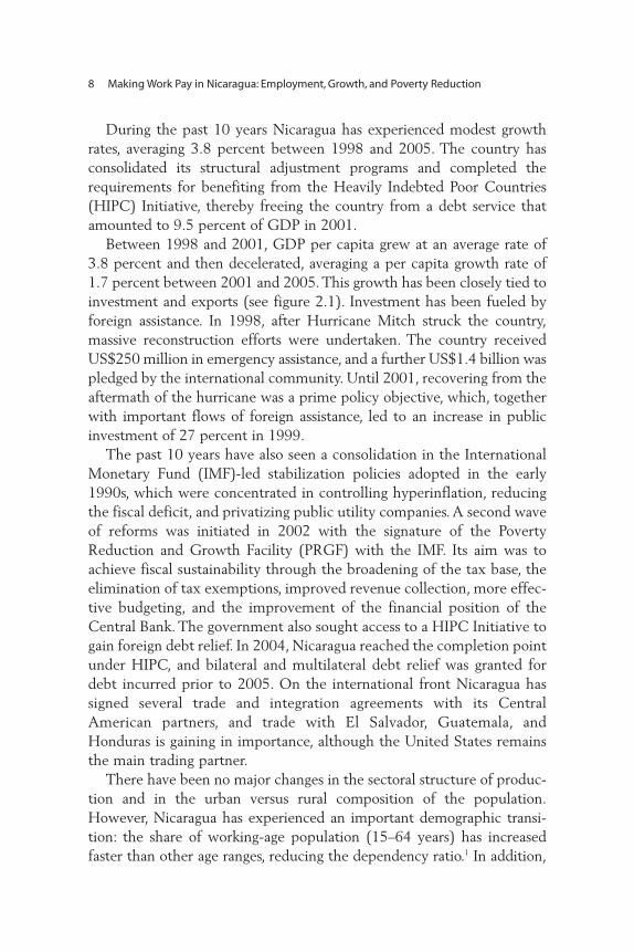
During the past 10 years Nicaragua has experienced modest growthrates, averaging 3.8 percent between 1998 and 2005. The country hasconsolidated its structural adjustment programs and completed therequirements for benefiting from the Heavily Indebted Poor Countries(HIPC) Initiative, thereby freeing the country from a debt service thatamounted to 9.5 percent of GDP in 2001.
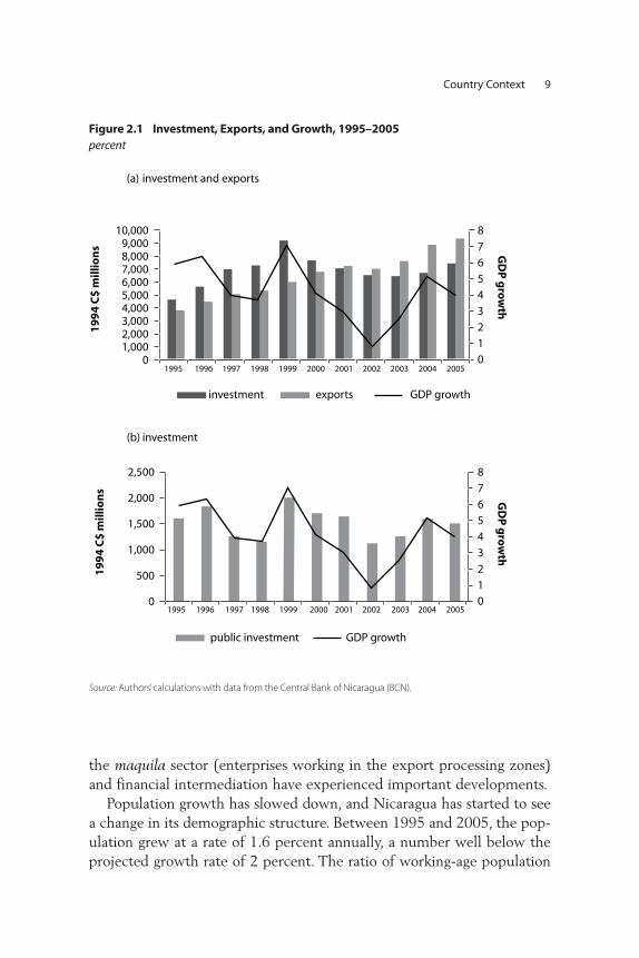
Between 1998 and 2001, GDP per capita grew at an average rate of3.8 percent and then decelerated, averaging a per capita growth rate of1.7 percent between 2001 and 2005. This growth has been closely tied toinvestment and exports (see figure 2.1). Investment has been fueled byforeign assistance. In 1998, after Hurricane Mitch struck the country,massive reconstruction efforts were undertaken. The country receivedUS$250 million in emergency assistance, and a further US$1.4 billion waspledged by the international community. Until 2001, recovering from theaftermath of the hurricane was a prime policy objective, which, togetherwith important flows of foreign assistance, led to an increase in publicinvestment of 27 percent in 1999.
The past 10 years have also seen a consolidation in the InternationalMonetary Fund (IMF)-led stabilization policies adopted in the early1990s, which were concentrated in controlling hyperinflation, reducingthe fiscal deficit, and privatizing public utility companies. A second waveof reforms was initiated in 2002 with the signature of the PovertyReduction and Growth Facility (PRGF) with the IMF. Its aim was toachieve fiscal sustainability through the broadening of the tax base, theelimination of tax exemptions, improved revenue collection, more effec-tive budgeting, and the improvement of the financial position of theCentral Bank. The government also sought access to a HIPC Initiative togain foreign debt relief. In 2004, Nicaragua reached the completion pointunder HIPC, and bilateral and multilateral debt relief was granted fordebt incurred prior to 2005. On the international front Nicaragua hassigned several trade and integration agreements with its CentralAmerican partners, and trade with El Salvador, Guatemala, andHonduras is gaining in importance, although the United States remainsthe main trading partner.
There have been no major changes in the sectoral structure of produc-tion and in the urban versus rural composition of the population.However, Nicaragua has experienced an important demographic transi-tion: the share of working-age population (15–64 years) has increasedfaster than other age ranges, reducing the dependency ratio.1 In addition,
Country Context 9
the maquila sector (enterprises working in the export processing zones)and financial intermediation have experienced important developments.
Population growth has slowed down, and Nicaragua has started to seea change in its demographic structure. Between 1995 and 2005, the pop-ulation grew at a rate of 1.6 percent annually, a number well below theprojected growth rate of 2 percent. The ratio of working-age population
public investment GDP growth
investment exports GDP growth
8
7
6
5
4
3
2
1
0
8
7
6
5
4
3
2
1
0
2,500
2,000
1,500
1,000
500
0
10,0009,0008,0007,0006,0005,0004,0003,0002,0001,000
0 1995 1996 1997 1998 1999 2000 2001 2002 2003 2004 2005
1995 1996 1997 1998 1999 2000 2001 2002 2003 2004 2005
(a) investment and exports
(b) investment
GD
P g
row
thG
DP
gro
wth
19
94
C$
mill
ion
s1
99
4 C
$ m
illio
ns
Figure 2.1 Investment, Exports, and Growth, 1995–2005percent
Source: Authors’calculations with data from the Central Bank of Nicaragua (BCN).
10 Making Work Pay in Nicaragua: Employment, Growth, and Poverty Reduction
(15–64 years) to total population increased from 53 percent in 1998 to55 percent in 2001 and 58 percent in 2005, significantly reducing thedependency ratio. Despite this overall demographic change, there was lit-tle gain in the share of urban population, which increased its share in totalpopulation by 1 percentage point in the past 10 years (table 2.1).
The sectoral structure of GDP remained relatively constant duringthese 10 years, with the secondary sector gaining only a 1-percentage-point share during the whole period. Although there were no majorchanges in the structure of production, within the secondary and tertiarysectors there were some important developments, namely the growth ofthe maquila sector and an important surge in financial intermediation.
Financial intermediation has grown at an average annual rate of 9 per-cent. This increase in intermediation is an important development, asNicaragua has the smallest banking system in Central America and as it isthe main source of credit for the private sector. Still, financial intermedi-ation is weak and accounts for only 3.6 percent of GDP.
Growth in the maquila sector has had important implications in termsof the availability of foreign reserves and employment. The maquila sec-tor, which started in the early 1990s with the development of the firstpublic free trade zone, has experienced an amazing dynamism. Between2001 and 2005, the share of maquila exports in total exports jumpedfrom 32 percent to 50 percent, and the sector generated just over 53,000new jobs during these four years. The value of transformation services inthe maquila, which measure, the value of domestic inputs used in theprocess, reached 5.5 percent of total value added in 2005.2
Labor Market Context
The labor market profile of Nicaragua is very similar to that of low-incomeand low-middle-income countries and is characterized by low unemploy-ment rates,3 low formality and wage employment rates, high shares of pop-ulation working in agriculture, and relatively high child labor.
This structure of employment is mainly a reflection of the stage ofindustrialization of these countries. Low- and middle-income countriesstill have a large agricultural sector in which productivity is generally lowand workers are mostly self-employed. Most of the population has verylow incomes, so they cannot afford to be unemployed. Instead, an impor-tant fraction of the working-age population is self-employed in informalactivities, many in agriculture. As industrialization progresses, the share of
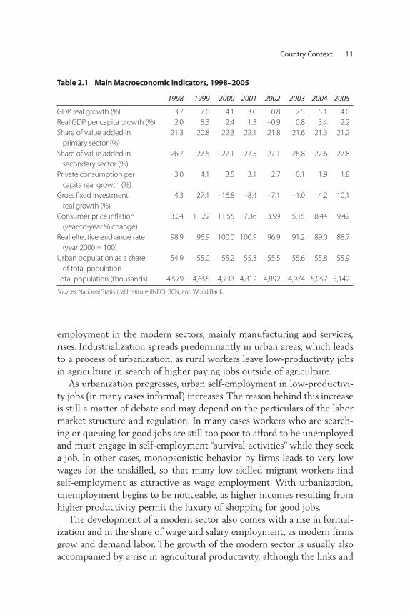
Table 2.1 Main Macroeconomic Indicators, 1998–2005
1998 1999 2000 2001 2002 2003 2004 2005
GDP real growth (%) 3.7 7.0 4.1 3.0 0.8 2.5 5.1 4.0Real GDP per capita growth (%) 2.0 5.3 2.4 1.3 –0.9 0.8 3.4 2.2Share of value added in 21.3 20.8 22.3 22.1 21.8 21.6 21.3 21.2
primary sector (%) Share of value added in 26.7 27.5 27.1 27.5 27.1 26.8 27.6 27.8
secondary sector (%)Private consumption per 3.0 4.1 3.5 3.1 2.7 0.1 1.9 1.8
capita real growth (%)Gross fixed investment 4.3 27.1 –16.8 –8.4 –7.1 –1.0 4.2 10.1
real growth (%)Consumer price inflation 13.04 11.22 11.55 7.36 3.99 5.15 8.44 9.42
(year-to-year % change)Real effective exchange rate 98.9 96.9 100.0 100.9 96.9 91.2 89.0 88.7
(year 2000 = 100)Urban population as a share 54.9 55.0 55.2 55.3 55.5 55.6 55.8 55.9
of total populationTotal population (thousands) 4,579 4,655 4,733 4,812 4,892 4,974 5,057 5,142
Sources: National Statistical Institute (INEC), BCN, and World Bank.
Country Context 11
employment in the modern sectors, mainly manufacturing and services,rises. Industrialization spreads predominantly in urban areas, which leadsto a process of urbanization, as rural workers leave low-productivity jobsin agriculture in search of higher paying jobs outside of agriculture.
As urbanization progresses, urban self-employment in low-productivi-ty jobs (in many cases informal) increases.The reason behind this increaseis still a matter of debate and may depend on the particulars of the labormarket structure and regulation. In many cases workers who are search-ing or queuing for good jobs are still too poor to afford to be unemployedand must engage in self-employment “survival activities” while they seeka job. In other cases, monopsonistic behavior by firms leads to very lowwages for the unskilled, so that many low-skilled migrant workers findself-employment as attractive as wage employment. With urbanization,unemployment begins to be noticeable, as higher incomes resulting fromhigher productivity permit the luxury of shopping for good jobs.
The development of a modern sector also comes with a rise in formal-ization and in the share of wage and salary employment, as modern firmsgrow and demand labor. The growth of the modern sector is usually alsoaccompanied by a rise in agricultural productivity, although the links and

12 Making Work Pay in Nicaragua: Employment, Growth, and Poverty Reduction
causalities for this are less clear. In many cases purposeful investment inagriculture frees rural labor, as more productive techniques mean thatfewer workers are needed to exploit the available land. This surplus labormigrates to urban markets, providing new labor that feeds the process ofurbanization and industrialization. In other cases, migration to nonagri-cultural jobs with higher productivity and higher pay allows householdsto generate savings that can translate into new investments that raise agri-cultural productivity.
As industrialization progresses child labor may decrease, as higherincomes mean lower opportunity costs of sending children to school.Additionally, as the demand for skill increases, so do its returns, and thebenefits of acquiring an education become more evident. Thus, it is cost-lier not to send children to school.
In Nicaragua, unemployment as defined by the International LabourOrganization (ILO) is low, slightly less than 4 percent (see table 2.2).Most of the employed work in the informal sector (82 percent), wageemployment accounts for half of the employed, agriculture absorbs a highshare of employment (37 percent), and child labor is relatively high (9percent). Agriculture is still a sector with low returns, and productivityhas been declining, suggesting that employment in this sector still acts asa “last resort” option for the working population. In the discussion thatfollows, the labor market structure is described in more detail.
Table 2.2 presents the main indicators of the labor market. It showsthat unemployment rates according to the ILO definition are very lowand that they remained almost constant during the period under analysis.The broad unemployment rate, which also includes discouraged workers,is slightly higher but is still low compared with other countries (less than10 percent). The working-age population, defined as those ages 15–64, asa proportion of the total population increased 5 percent (or 3 percentagepoints). The number of employed as a fraction of the total working-agepopulation also rose slightly. Child labor saw a small increase, from 8.7percent to 9.2 percent. The poverty rate among unemployed workersstands out, at half the overall poverty rate, which suggests that unemploy-ment is not strongly correlated with poverty.
The table also shows the number of workers affiliated with social secu-rity, which is often a measure for formalization. In Nicaragua only some 19percent of the labor force has social security, and this ratio decreasedslightly in 2005. Finally, the table shows the number of workers holdingmore than one job concurrently. It has been pointed out that in many cases
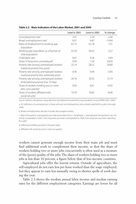
workers cannot generate enough income from their main job and mustfind additional work to complement their income, so that the share ofworkers holding two or more jobs concurrently is often used as a measureof the (poor) quality of the jobs.The share of workers holding two or morejobs is less than 10 percent, a figure below that of low-income countries.
Agricultural jobs offer the lowest returns. Outside of agriculture, theself-employed do not earn less per hour worked than the wage employed,but they appear to earn less annually owing to shorter spells of work dur-ing the year.
Table 2.3 shows the median annual labor income and median earningrates for the different employment categories. Earnings are lower for all
Country Context 13
Table 2.2 Main Indicators of the Labor Market, 2001 and 2005
Level in 2001 Level in 2005 % change
Unemployment ratea 3.47 3.39 –2.44Broad unemployment rateb 8.07 6.87 –14.84Ratio of employment to working-age 62.15 62.78 1.01
populationWorking-age population as a fraction of 55.30 58.22 5.27
total populationChild labor rate 8.87 9.28 4.69Share of long-term unemployedc 0.04 1.50 3,650Poverty rate among unemployed workers 22.14 28.52 28.80
(national poverty line, poor)Poverty rate among unemployed workers 6.96 6.69 –3.83
(national poverty line, extremely poor)Poverty rate among unemployed workers 24.76 28.52 15.19
(international poverty line, 1$/day)Share of workers holding two or more 9.03 8.41 –6.92
jobs concurrentlyd
Share of workers affiliated with 19.70 18.05 –8.40social securitye
Source: Authors’calculations using data from the National Household Living Standards Survey (EMNV 2001, 2005).
a. ILO definition of unemployment is those who are not employed but who actively searched for a job in the pastweek.
b. Broad unemployment rate also includes discouraged workers.
c. Ratio of long-term unemployed over total active labor force = (employed + unemployed), the questions are notstrictly comparable: in 2001, How long have you been unemployed? In 2005, How long have you been searchingfor a job?
d. Defined as holding two jobs in the past week.
e. Affiliated with social security in main occupation.

14 Making Work Pay in Nicaragua: Employment, Growth, and Poverty ReductionTa
ble
2.3
Earn
ings
and
Inco
me
by E
mpl
oym
ent C
ateg
ory,
200
1 an
d 20
05
Leve
l in
2001
Leve
l in
2005
% c
hang
e
Non
agric
ultu
reAg
ricul
ture
Non
agric
ultu
reAg
ricul
ture
Non
agric
ultu
reAg
ricul
ture
Wag
e an
d s
alar
y w
orke
rsM
edia
n an
nual
labo
r inc
ome
21,0
64.3
610
,532
.18
20,8
44.0
011
,700
.00
–1.0
511
.09
Med
ian
hour
ly e
arni
ngs
rate
8.32
4.22
8.52
5.06
2.41
20.0
1Lo
w e
arni
ngs
rate
20.5
737
.76
17.6
624
.86
–14.
17–3
4.16
Ind
ivid
ual
sel
f-em
plo
yed
wor
kers
Med
ian
annu
al la
bor i
ncom
e13
,374
.20
6,42
3.42
12,0
00.0
06,
319.
25–1
0.28
–1.6
2M
edia
n ho
urly
ear
ning
s ra
te11
.20
3.88
6.22
—–4
4.43
—Lo
w e
arni
ngs
rate
28.3
255
.96
34.1
351
.59
20.5
0–7
.81
Emp
loye
rsM
edia
n an
nual
labo
r inc
ome
46,8
09.7
09,
298.
0045
,000
.00
31,7
51.1
9–3
.87
241.
48M
edia
n ho
urly
ear
ning
s ra
te26
.87
5.87
19.7
8—
–26.
39—
Low
ear
ning
s ra
te3.
4045
.72
6.83
9.72
100.
85–7
8.74
Hou
seh
old
en
terp
rise
wor
kers
Med
ian
annu
al la
bor i
ncom
e10
,532
.18
5,19
0.74
16,0
53.4
55,
891.
4452
.42
13.5
0M
edia
n ho
urly
ear
ning
s ra
te10
.75
4.12
8.40
——
—Lo
w e
arni
ngs
rate
23.4
064
.36
56.9
557
.70
143.
36–1
0.34
Sour
ce: A
utho
rs’c
alcu
latio
ns w
ith d
ata
from
EM
NV
2001
and
200
5.
Not
e: —
indi
cate
s in
suffi
cien
t or m
issin
g da
ta. M
edia
n an
nual
labo
r inc
ome
refe
rs to
all
the
occu
patio
ns a
nd in
clud
es m
onet
ary,
nonm
onet
ary,
and
in-k
ind
earn
ings
. The
med
ian
hour
ly e
arn-
ings
rate
is c
alcu
late
d fro
m th
e m
ain
occu
patio
n on
ly, e
xcep
t for
the
agric
ultu
ral s
elf-e
mpl
oyed
, agr
icul
tura
l em
ploy
ers,
and
agric
ultu
ral f
amily
ent
erpr
ises,
for w
hich
it is
cal
cula
ted
as p
rofit
spe
r hou
r wor
ked
usin
g th
e ag
ricul
tura
l ent
erpr
ise m
odul
e. In
200
5, th
e ag
ricul
tura
l ent
erpr
ise m
odul
e di
d no
t rep
ort h
ours
wor
ked,
and
ther
efor
e th
e ho
urly
ear
ning
s ra
te c
anno
t be
calc
ulat
-ed
for t
he s
elf-e
mpl
oyed
in a
gric
ultu
re.
agricultural categories, and among agricultural workers the lowest incomeis obtained by household enterprise workers and the individually self-employed. It is also obvious that wages decreased for nonagriculturalemployment while they increased for agricultural workers. The self-employed in nonagricultural work have similar earning rates to the wageemployed, which suggests that wage employment is not necessarily a bet-ter earning option. However, yearly earnings among the self-employed arelower, which suggests that they are employed for shorter periods or workfewer hours.
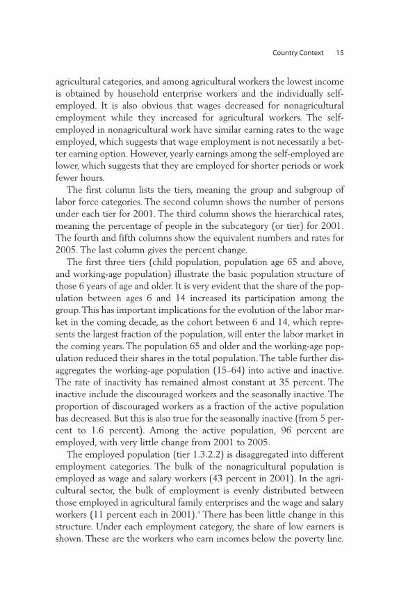
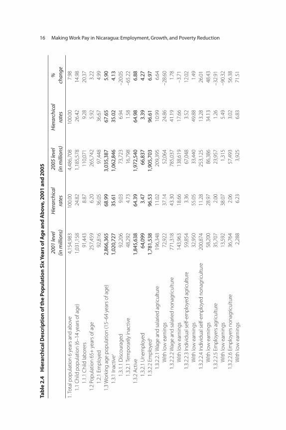
The first column lists the tiers, meaning the group and subgroup oflabor force categories. The second column shows the number of personsunder each tier for 2001. The third column shows the hierarchical rates,meaning the percentage of people in the subcategory (or tier) for 2001.The fourth and fifth columns show the equivalent numbers and rates for2005. The last column gives the percent change.
The first three tiers (child population, population age 65 and above,and working-age population) illustrate the basic population structure ofthose 6 years of age and older. It is very evident that the share of the pop-ulation between ages 6 and 14 increased its participation among thegroup.This has important implications for the evolution of the labor mar-ket in the coming decade, as the cohort between 6 and 14, which repre-sents the largest fraction of the population, will enter the labor market inthe coming years. The population 65 and older and the working-age pop-ulation reduced their shares in the total population. The table further dis-aggregates the working-age population (15–64) into active and inactive.The rate of inactivity has remained almost constant at 35 percent. Theinactive include the discouraged workers and the seasonally inactive. Theproportion of discouraged workers as a fraction of the active populationhas decreased. But this is also true for the seasonally inactive (from 5 per-cent to 1.6 percent). Among the active population, 96 percent areemployed, with very little change from 2001 to 2005.
The employed population (tier 1.3.2.2) is disaggregated into differentemployment categories. The bulk of the nonagricultural population isemployed as wage and salary workers (43 percent in 2001). In the agri-cultural sector, the bulk of employment is evenly distributed betweenthose employed in agricultural family enterprises and the wage and salaryworkers (11 percent each in 2001).4 There has been little change in thisstructure. Under each employment category, the share of low earners isshown. These are the workers who earn incomes below the poverty line.
Country Context 15
Tabl
e 2.
4H
iera
rchi
cal D
escr
iptio
n of
the
Popu
latio
n Si
x Ye
ars o
f Age
and
Abo
ve, 2
001
and
2005
2001
leve
l H
iera
rchi
cal
2005
leve
l H
iera
rchi
cal
%
(in m
illio
ns)
rate
s(in
mill
ions
)ra
tes
chan
ge
1. To
tal p
opul
atio
n 6
year
s an
d ab
ove
4,15
4,98
310
0.00
4,48
6,70
810
0.00
7.98
1.1
Child
pop
ulat
ion
(6–1
4 ye
ars
of a
ge)
1,03
1,15
824
.82
1,18
5,57
826
.42
14.9
81.
1.1
Child
labo
rers
91,4
438.
8711
0,07
19.
2820
.37
1.2
Popu
latio
n 65
+ y
ears
of a
ge25
7,45
96.
2026
5,74
25.
923.
221.
2.1
Empl
oyed
92,8
1636
.05
97,4
4836
.67
4.99
1.3
Wor
king
age
pop
ulat
ion
(15–
64 y
ears
of a
ge)
2,86
6,36
568
.99
3,03
5,38
767
.65
5.90
1.3.
1 In
activ
ea1,
020,
727
35.6
11,
062,
846
35.0
24.
131.
3.1.
1 D
iscou
rage
d92
,206
9.03
73,7
236.
94–2
0.05
1.3.
2.1
Tem
pora
rily
inac
tive
48,2
924.
7316
,798
1.58
–65.
221.
3.2
Activ
e1,
845,
638
64.3
91,
972,
540
64.9
86.
881.
3.2.
1 U
nem
ploy
ed64
,099
3.47
66,8
373.
394.
271.
3.2.
2 Em
ploy
edb
1,78
1,53
896
.53
1,90
5,70
396
.61
6.97
1.3.
2.2.
1 W
age
and
sala
ried
agric
ultu
re
196,
348
11.0
220
9,39
510
.99
6.64
With
low
ear
ning
s72
,922
37.1
452
,064
24.8
6–2
8.60
1.3.
2.2.
2 W
age
and
sala
ried
nona
gric
ultu
re77
1,31
843
.30
785,
037
41.1
91.
78W
ith lo
w e
arni
ngs
143,
963
18.6
613
8,61
917
.66
–3.7
11.
3.2.
2.3
Indi
vidu
al s
elf-e
mpl
oyed
agr
icul
ture
59,8
543.
3667
,048
3.52
12.0
2W
ith lo
w e
arni
ngs
32,9
5055
.05
33,4
4049
.88
1.49
1.3.
2.2.
4 In
divi
dual
sel
f-em
ploy
ed n
onag
ricul
ture
200,
874
11.2
825
3,12
513
.28
26.0
1W
ith lo
w e
arni
ngs
58,2
0028
.97
86,3
8634
.13
48.4
31.
3.2.
2.5
Empl
oyer
s ag
ricul
ture
35,7
072.
0023
,957
1.26
–32.
91W
ith lo
w e
arni
ngs
13,5
9238
.07
1,31
55.
49–9
0.32
1.3.
2.2.
6 Em
ploy
ers
nona
gric
ultu
re36
,764
2.06
57,4
933.
0256
.38
With
low
ear
ning
s2,
288
6.23
3,92
56.
8371
.51
16 Making Work Pay in Nicaragua: Employment, Growth, and Poverty Reduction

Country Context 1720
01 le
vel
Hie
rarc
hica
l 20
05 le
vel
Hie
rarc
hica
l %
(in
mill
ions
)ra
tes
(in m
illio
ns)
rate
sCh
ange
1.3.
2.2.
7 In
hou
seho
ld e
nter
prise
s ag
ricul
ture
c19
3,37
710
.85
300,
639
15.7
855
.47
With
low
ear
ning
s79
,136
40.9
294
,246
31.3
519
.09
1.3.
2.2.
8 In
hou
seho
ld e
nter
prise
s no
nagr
icul
ture
c12
2,00
76.
8518
3,94
99.
6550
.77
With
low
ear
ning
s32
,071
26.2
910
4,76
356
.95
226.
661.
3.2.
2.9
Oth
ers
165,
286
9.28
25,0
551.
31–1
69.2
0
Sour
ce: A
utho
rs’c
alcu
latio
ns w
ith d
ata
from
EM
NV
2001
and
200
5.
a. T
he s
urve
y do
es n
ot a
llow
for a
dist
inct
ion
betw
een
disc
oura
ged
wor
kers
who
are
will
ing
to w
ork
and
thos
e w
ho a
re n
ot. T
empo
raril
y in
activ
e w
orke
rs a
re th
ose
wai
ting
to s
tart
a jo
b or
wai
ting
for t
he h
arve
st s
easo
n to
beg
in.
b. E
mpl
oyed
wor
kers
are
sub
clas
sifie
d ac
cord
ing
to th
e m
ain
occu
patio
n. T
he c
ateg
ory
does
not
sum
to to
tal e
mpl
oyed
bec
ause
oth
er e
mpl
oyed
are
cla
ssifi
ed a
s m
embe
rs o
f coo
pera
tive
ente
rpris
es.
c. In
clud
es u
npai
d fa
mily
mem
bers
.
The highest number of low earners can be found among those individu-ally self-employed in agriculture (55 percent have low earnings) andthose that work in household family enterprises in agriculture (40 per-cent have low earnings). Employment in all agricultural categories hasincreased. As will be discussed further, it is unclear how much of thisincrease might be due to errors in the urban-rural weights of the 2001survey.
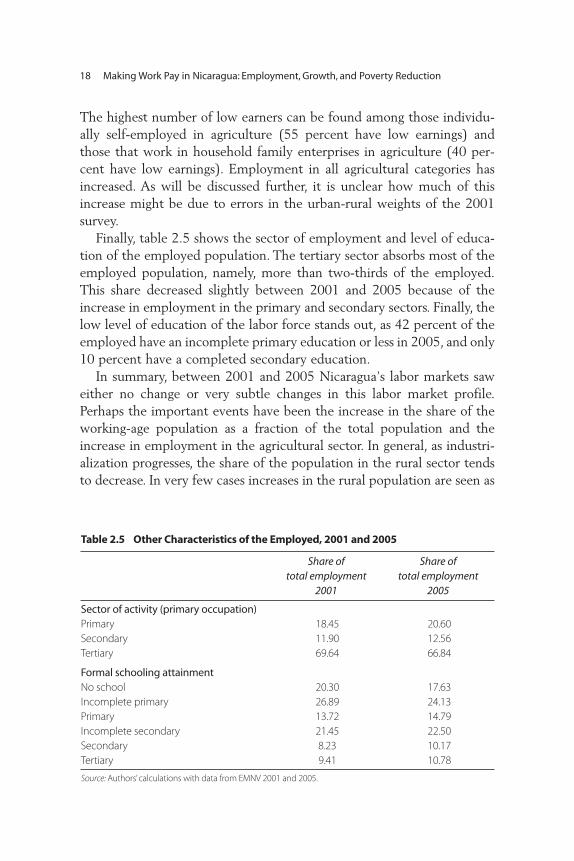
Finally, table 2.5 shows the sector of employment and level of educa-tion of the employed population. The tertiary sector absorbs most of theemployed population, namely, more than two-thirds of the employed.This share decreased slightly between 2001 and 2005 because of theincrease in employment in the primary and secondary sectors. Finally, thelow level of education of the labor force stands out, as 42 percent of theemployed have an incomplete primary education or less in 2005, and only10 percent have a completed secondary education.
In summary, between 2001 and 2005 Nicaragua’s labor markets saweither no change or very subtle changes in this labor market profile.Perhaps the important events have been the increase in the share of theworking-age population as a fraction of the total population and theincrease in employment in the agricultural sector. In general, as industri-alization progresses, the share of the population in the rural sector tendsto decrease. In very few cases increases in the rural population are seen as
18 Making Work Pay in Nicaragua: Employment, Growth, and Poverty Reduction
Table 2.5 Other Characteristics of the Employed, 2001 and 2005
Share of Share of total employment total employment
2001 2005
Sector of activity (primary occupation)Primary 18.45 20.60Secondary 11.90 12.56Tertiary 69.64 66.84
Formal schooling attainmentNo school 20.30 17.63Incomplete primary 26.89 24.13Primary 13.72 14.79Incomplete secondary 21.45 22.50Secondary 8.23 10.17Tertiary 9.41 10.78
Source: Authors’calculations with data from EMNV 2001 and 2005.

a response to urban crisis. However, this has not been the case inNicaragua; thus the reason for this increase is yet to be determined. Onepossible explanation is that the population weights used in the 2001 sur-vey were not in accordance with the census behavior of the population(see box 2.1). However, it is not clear to what extent this may be affect-ing the results.
Country Context 19
Box 2.1
Urban versus Rural Population: Possible Data Problems
The table below shows the population calculated from the census and the sur-
veys. According to the surveys, urban population increased substantially from
1998 to 2001, from 54 percent to 58 percent, and then decreased between 2001
and 2005, from 58 percent to 55 percent. It is hard to estimate whether the be-
havior in the surveys is actually true. It is surprising that urbanization increased
substantially and then reversed in such a short time. The available census infor-
mation suggests that there was an increase of 1 percentage point between 1995
and 2005, but there are no data points in between to illustrate the intercensus
behavior. Moreover, the 2001 population estimations used in the 2001 survey
overestimate the population growth. The present report corrects the weights for
this overestimation but makes no adjustments for regional or urban-rural com-
position, as no data were available to do that. It is unlikely that the population
overestimation was uniform across regions or urban and rural populations.
Percentage of regional populationCensus Survey
1995 2005 1998 2001 2005Managua 25.10 24.56 26.06 24.83 24.54
Pacific Urban 17.38 17.13 16.75 17.37 16.95
Pacific Rural 14.16 12.34 15.57 14.34 12.38
Central Urban 10.79 12.21 10.51 12.74 12.28
Central Rural 20.30 19.83 20.82 18.67 19.85
Atlantic Urban 3.89 4.37 5.05 5.50 4.39
Atlantic Rural 8.39 9.56 5.25 6.55 9.62
Overall Urban 54.41 55.92 54.35 58.33 55.83

Labor Regulation in Nicaragua
The largest share of nonlabor costs paid by employers corresponds tosocial security contributions, which amount to 15 percent of the wage.Workers contribute 6.25 percent of their wage for social security.Workersare entitled to one month of paid vacations and an annual bonus that isequivalent to one month of work. They are also entitled to senioritybonuses. In addition to these costs, employers have to pay 2 percent of thetotal payroll for INATEC, the technological training institute. Moreover,there are minimum wages, by sectors, and strong support for unioniza-tion. Firms are allowed to hire temporary workers and can extend thistype of contract indefinitely. The workweek consists of six days and it canbe extended up to 50 hours. Termination of the employment contract isauthorized with no third-party involvement, and workers are entitled toseverance pay upon termination, which varies with tenure.
Nicaragua conducted an enterprise survey for 2003, in conjunctionwith the World Bank. Enterprise surveys collect information among firmsregarding constraints to growth and business activities.5 The informationis often used for the analysis of the investment climate in different coun-tries. Although a complete investment climate assessment is outside thescope of this report, the survey can be used to pinpoint the main bottle-necks that are present and that may be hampering growth and employ-ment generation.
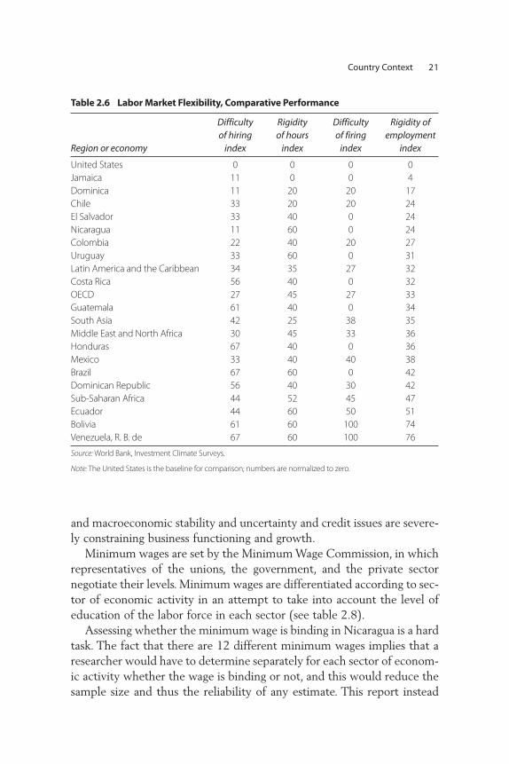
The information collected includes the level of nonwage labor costsand the perception among firms of the rigidity of labor regulation. Usingthis information, the Enterprise Survey Unit at the International FinanceCorporation constructs relative hiring and firing rigidity indexes. Table2.6 compares the results for Nicaragua with other countries in the region(and elsewhere) and with its main trading partners (shown in gray). Ascan be seen, Nicaragua does not appear particularly rigid when comparedwith other countries in the region. In fact, it appears to be one of the leastrigid economies, ranking only below Jamaica and the DominicanRepublic and having an overall performance equal to Chile’s and ElSalvador’s. It is relatively low compared with the United States, one of itsmain trading partners but also the most flexible economy in the world.
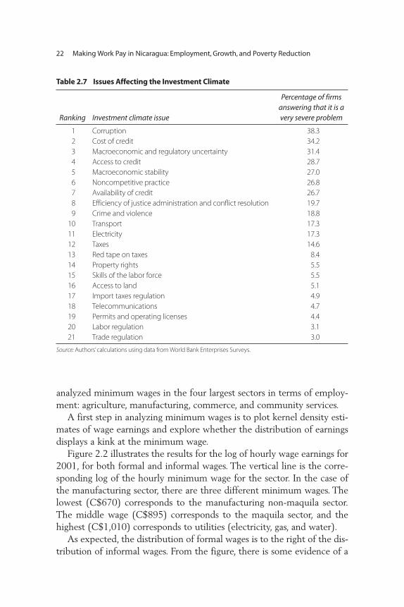
Other information collected can be used to asses the main constraintsto investment faced by different firms. Table 2.7 shows the percentage offirms responding that a particular constraint was severely hampering busi-ness functioning and growth. Responses show that labor regulation andthe skills of the labor force are among the least problematic constraints,
20 Making Work Pay in Nicaragua: Employment, Growth, and Poverty Reduction
and macroeconomic stability and uncertainty and credit issues are severe-ly constraining business functioning and growth.
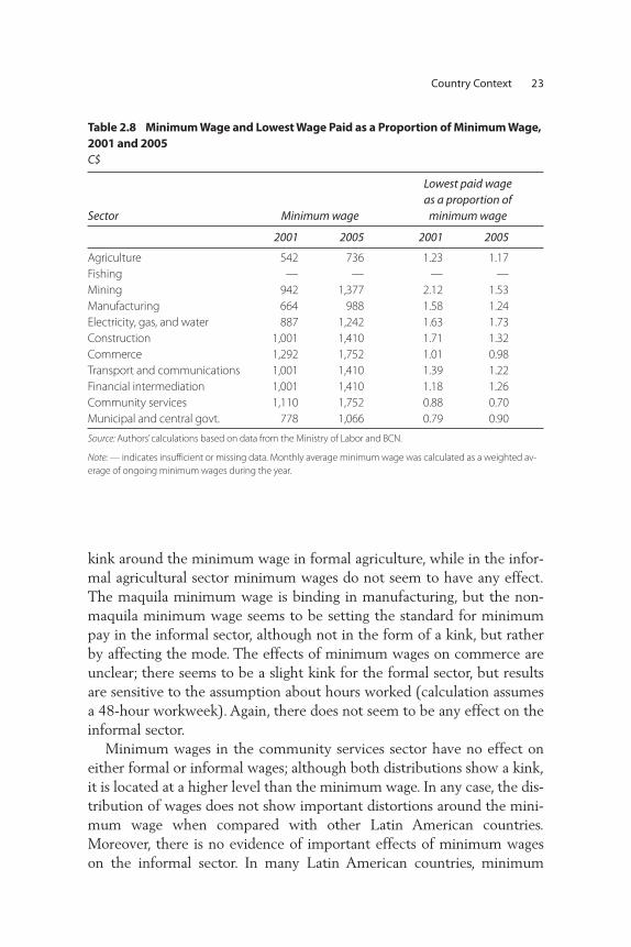
Minimum wages are set by the Minimum Wage Commission, in whichrepresentatives of the unions, the government, and the private sectornegotiate their levels. Minimum wages are differentiated according to sec-tor of economic activity in an attempt to take into account the level ofeducation of the labor force in each sector (see table 2.8).
Assessing whether the minimum wage is binding in Nicaragua is a hardtask. The fact that there are 12 different minimum wages implies that aresearcher would have to determine separately for each sector of econom-ic activity whether the wage is binding or not, and this would reduce thesample size and thus the reliability of any estimate. This report instead
Country Context 21
Table 2.6 Labor Market Flexibility, Comparative Performance
Difficulty Rigidity Difficulty Rigidity of of hiring of hours of firing employment
Region or economy index index index index
United States 0 0 0 0Jamaica 11 0 0 4Dominica 11 20 20 17Chile 33 20 20 24El Salvador 33 40 0 24Nicaragua 11 60 0 24Colombia 22 40 20 27Uruguay 33 60 0 31Latin America and the Caribbean 34 35 27 32Costa Rica 56 40 0 32OECD 27 45 27 33Guatemala 61 40 0 34South Asia 42 25 38 35Middle East and North Africa 30 45 33 36Honduras 67 40 0 36Mexico 33 40 40 38Brazil 67 60 0 42Dominican Republic 56 40 30 42Sub-Saharan Africa 44 52 45 47Ecuador 44 60 50 51Bolivia 61 60 100 74Venezuela, R. B. de 67 60 100 76
Source: World Bank, Investment Climate Surveys.
Note: The United States is the baseline for comparison; numbers are normalized to zero.
analyzed minimum wages in the four largest sectors in terms of employ-ment: agriculture, manufacturing, commerce, and community services.
A first step in analyzing minimum wages is to plot kernel density esti-mates of wage earnings and explore whether the distribution of earningsdisplays a kink at the minimum wage.
Figure 2.2 illustrates the results for the log of hourly wage earnings for2001, for both formal and informal wages. The vertical line is the corre-sponding log of the hourly minimum wage for the sector. In the case ofthe manufacturing sector, there are three different minimum wages. Thelowest (C$670) corresponds to the manufacturing non-maquila sector.The middle wage (C$895) corresponds to the maquila sector, and thehighest (C$1,010) corresponds to utilities (electricity, gas, and water).
As expected, the distribution of formal wages is to the right of the dis-tribution of informal wages. From the figure, there is some evidence of a
22 Making Work Pay in Nicaragua: Employment, Growth, and Poverty Reduction
Table 2.7 Issues Affecting the Investment Climate
Percentage of firms answering that it is a
Ranking Investment climate issue very severe problem
1 Corruption 38.32 Cost of credit 34.23 Macroeconomic and regulatory uncertainty 31.44 Access to credit 28.75 Macroeconomic stability 27.06 Noncompetitive practice 26.87 Availability of credit 26.78 Efficiency of justice administration and conflict resolution 19.79 Crime and violence 18.8
10 Transport 17.311 Electricity 17.312 Taxes 14.613 Red tape on taxes 8.414 Property rights 5.515 Skills of the labor force 5.516 Access to land 5.117 Import taxes regulation 4.918 Telecommunications 4.719 Permits and operating licenses 4.420 Labor regulation 3.121 Trade regulation 3.0
Source: Authors’calculations using data from World Bank Enterprises Surveys.
kink around the minimum wage in formal agriculture, while in the infor-mal agricultural sector minimum wages do not seem to have any effect.The maquila minimum wage is binding in manufacturing, but the non-maquila minimum wage seems to be setting the standard for minimumpay in the informal sector, although not in the form of a kink, but ratherby affecting the mode. The effects of minimum wages on commerce areunclear; there seems to be a slight kink for the formal sector, but resultsare sensitive to the assumption about hours worked (calculation assumesa 48-hour workweek). Again, there does not seem to be any effect on theinformal sector.
Minimum wages in the community services sector have no effect oneither formal or informal wages; although both distributions show a kink,it is located at a higher level than the minimum wage. In any case, the dis-tribution of wages does not show important distortions around the mini-mum wage when compared with other Latin American countries.Moreover, there is no evidence of important effects of minimum wageson the informal sector. In many Latin American countries, minimum
Country Context 23
Table 2.8 Minimum Wage and Lowest Wage Paid as a Proportion of Minimum Wage,2001 and 2005C$
Lowest paid wage as a proportion of
Sector Minimum wage minimum wage
2001 2005 2001 2005
Agriculture 542 736 1.23 1.17Fishing — — — —Mining 942 1,377 2.12 1.53Manufacturing 664 988 1.58 1.24Electricity, gas, and water 887 1,242 1.63 1.73Construction 1,001 1,410 1.71 1.32Commerce 1,292 1,752 1.01 0.98Transport and communications 1,001 1,410 1.39 1.22Financial intermediation 1,001 1,410 1.18 1.26Community services 1,110 1,752 0.88 0.70Municipal and central govt. 778 1,066 0.79 0.90
Source: Authors’calculations based on data from the Ministry of Labor and BCN.
Note: — indicates insufficient or missing data. Monthly average minimum wage was calculated as a weighted av-erage of ongoing minimum wages during the year.
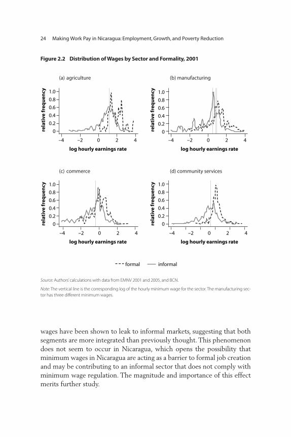
wages have been shown to leak to informal markets, suggesting that bothsegments are more integrated than previously thought. This phenomenondoes not seem to occur in Nicaragua, which opens the possibility thatminimum wages in Nicaragua are acting as a barrier to formal job creationand may be contributing to an informal sector that does not comply withminimum wage regulation. The magnitude and importance of this effectmerits further study.
24 Making Work Pay in Nicaragua: Employment, Growth, and Poverty Reduction
formal informal
(a) agriculture
(c) commerce
(b) manufacturing
(d) community services
1.0
0.8
0.6
0.4
0.2
0
1.0
0.8
0.6
0.4
0.2
0
1.0
0.8
0.6
0.4
0.2
0
1.0
0.8
0.6
0.4
0.2
0
–4 –2 0 2 4 –4 –2 0 2 4
–4 –2 0 2 4 –4 –2 0 2 4
log hourly earnings rate log hourly earnings rate
log hourly earnings rate log hourly earnings rate
rela
tive
freq
uen
cyre
lati
ve fr
equ
ency
rela
tive
freq
uen
cyre
lati
ve fr
equ
ency
Figure 2.2 Distribution of Wages by Sector and Formality, 2001
Source: Authors’calculations with data from EMNV 2001 and 2005, and BCN.
Note: The vertical line is the corresponding log of the hourly minimum wage for the sector. The manufacturing sec-tor has three different minimum wages.

It is unclear whether the current structure of minimum wages pro-vides much benefit over a unique minimum wage. If the idea of sectoralminimum wages is to take into account the different average skill levelsof the labor force in each sector, it might be better to set a minimumwage by level of education (for the low skilled) rather than by sector.Thecurrent structure of the minimum wage might be introducing unneces-sary distortions into the labor market, and might be segmenting the mar-ket according to skills. This might explain the behavior of maquila facto-ries, which face a higher minimum wage than overall manufacturing and,as a response, may restrict employment to those with a secondary orhigher education. If the analysis assumes that more productive firmshave larger profits and a higher share of skills (as is often the case), thecurrent minimum wage–setting mechanism is acting more as a centralcollective bargaining mechanism to distribute profits between low-skilled workers and firms, rather than as a mechanism for setting thelowest paid wage. But even if this were the objective of having a differ-ential minimum wage by sectors, it is unclear what the advantages of thiscentralized bargaining system would be over a decentralized (firm level)bargaining system.
When firms make hiring decisions they compare the marginal cost oflabor, that is, the minimum wage, with the marginal product, that is, thevalue of output produced by one additional worker. More productivefirms are usually more competitive, account for larger shares of employ-ment, and grow faster. If firms differ in productivity, and minimum wagesare higher for the most productive firms, then low-skilled workers (forwhich minimum wages are binding) will be excluded from the mostdynamic and productive sectors of the economy. Instead, a minimumwage by skill level will mean that more productive firms will have anadvantage with respect to low-productivity firms when hiring low-skilledworkers. Relative to the marginal cost (that is, the minimum wage), themarginal benefit of having an unskilled worker is larger. Therefore, high-productivity firms might be more inclined to increase the use of unskilledlabor (that is, increase the unskilled-labor intensity of the productionprocess), while workers will be equally off (for a given level of education)in any sector or firm. Understanding the employment effects of minimumwages and the impact of its sectoral structure on employment, plus therelative demand for unskilled labor, is beyond the scope of this report. Butit is an area that merits further research.
Country Context 25

Notes
1. The dependency ratio is the ratio of total population to working age popula-tion, and it indicates, on average, how many people a working adult has to sup-port.
2. The value of transformation services corresponds to the difference betweenthe value of imported raw materials and the value of final exports and corre-sponds mostly with the cost of labor and utilities.
3. ILO defines unemployed as those who are not employed and who actuallylooked for a job in the past week.
4. The individually self-employed are the self-employed who do not work withother family members. The employers are those who are self-employed buthave paid workers. The household enterprise workers are the self-employedwho work with unpaid family members or unpaid helpers.
5. The International Finance Corporation of the World Bank Group providescomprehensive data for productivity analysis in emerging markets at itsEnterprise Surveys Web site: http://www.enterprisesurveys.org/.
26 Making Work Pay in Nicaragua: Employment, Growth, and Poverty Reduction
This chapter describes the labor and productivity profile of growth andlinks it to poverty reduction. It also takes a closer look at the manufactur-ing sector and the maquila sector. The first section describes the maintrends in output, poverty, and employment; the second section decom-poses growth into sectoral employment and productivity changes; thefinal section takes a closer look at manufacturing.
Main Trends in Output
Value added grew at an average annual rate of 4.2 percent between 1998and 2005. Between 1998 and 2001 growth reached 5.42 percent. Growthdecelerated dramatically between 2001 and 2005, reaching an averageannual growth rate of 3.24 percent (table 3.1). Agriculture, construction,and services suffered the largest growth losses. Only transport and thefinancial sector kept their growth pace, but these sectors are small in termsof employment and output. Furthermore, the share of the poor employedin these two sectors is less than 4 percent. Despite this strong decelerationof economic activity, the manufacturing sector managed to grow at anaverage annual rate of 4.4 percent. This has important implications forpoverty reduction, as discussed later. Overall growth was fueled in part by
C H A P T E R 3
Output, Population, Employment, and Poverty
27
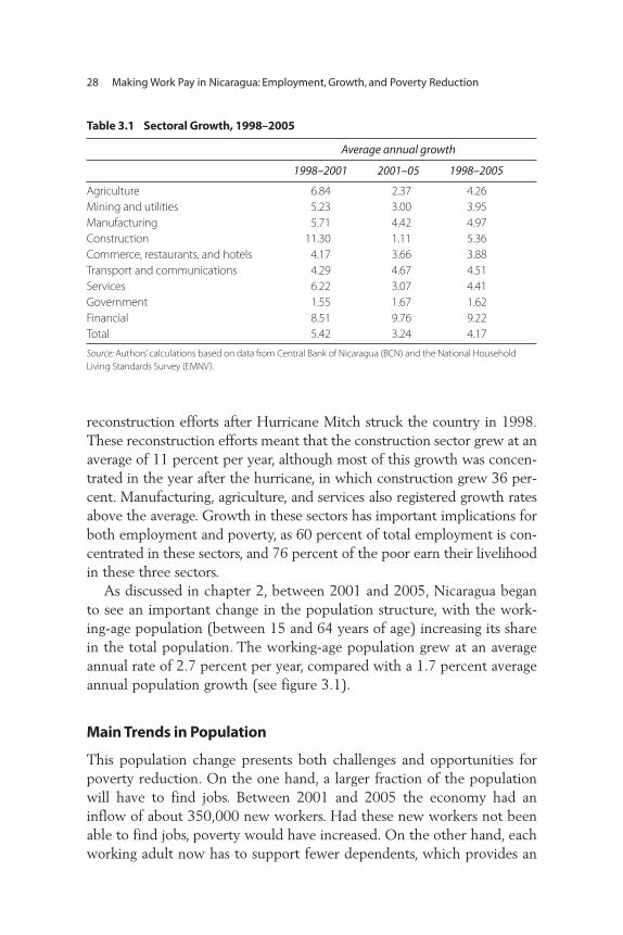
reconstruction efforts after Hurricane Mitch struck the country in 1998.These reconstruction efforts meant that the construction sector grew at anaverage of 11 percent per year, although most of this growth was concen-trated in the year after the hurricane, in which construction grew 36 per-cent. Manufacturing, agriculture, and services also registered growth ratesabove the average. Growth in these sectors has important implications forboth employment and poverty, as 60 percent of total employment is con-centrated in these sectors, and 76 percent of the poor earn their livelihoodin these three sectors.
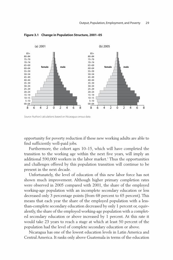
As discussed in chapter 2, between 2001 and 2005, Nicaragua beganto see an important change in the population structure, with the work-ing-age population (between 15 and 64 years of age) increasing its sharein the total population. The working-age population grew at an averageannual rate of 2.7 percent per year, compared with a 1.7 percent averageannual population growth (see figure 3.1).
Main Trends in Population
This population change presents both challenges and opportunities forpoverty reduction. On the one hand, a larger fraction of the populationwill have to find jobs. Between 2001 and 2005 the economy had aninflow of about 350,000 new workers. Had these new workers not beenable to find jobs, poverty would have increased. On the other hand, eachworking adult now has to support fewer dependents, which provides an
28 Making Work Pay in Nicaragua: Employment, Growth, and Poverty Reduction
Table 3.1 Sectoral Growth, 1998–2005
Average annual growth
1998–2001 2001–05 1998–2005
Agriculture 6.84 2.37 4.26Mining and utilities 5.23 3.00 3.95Manufacturing 5.71 4.42 4.97Construction 11.30 1.11 5.36Commerce, restaurants, and hotels 4.17 3.66 3.88Transport and communications 4.29 4.67 4.51Services 6.22 3.07 4.41Government 1.55 1.67 1.62Financial 8.51 9.76 9.22Total 5.42 3.24 4.17
Source: Authors’calculations based on data from Central Bank of Nicaragua (BCN) and the National Household Living Standards Survey (EMNV).
opportunity for poverty reduction if these new working adults are able tofind sufficiently well-paid jobs.
Furthermore, the cohort ages 10–15, which will have completed thetransition to the working age within the next five years, will imply anadditional 590,000 workers in the labor market.1 Thus the opportunitiesand challenges offered by this population transition will continue to bepresent in the next decade.
Unfortunately, the level of education of this new labor force has notshown much improvement. Although higher primary completion rateswere observed in 2005 compared with 2001, the share of the employedworking-age population with an incomplete secondary education or lessdecreased only 3 percentage points (from 68 percent to 65 percent). Thismeans that each year the share of the employed population with a less-than-complete secondary education decreased by only 1 percent or, equiv-alently, the share of the employed working-age population with a complet-ed secondary education or above increased by 1 percent. At this rate itwould take 23 years to reach a stage at which at least 50 percent of thepopulation had the level of complete secondary education or above.
Nicaragua has one of the lowest education levels in Latin America andCentral America. It ranks only above Guatemala in terms of the education
Output, Population, Employment, and Poverty 29
(a) 2001 (b) 2005
8 6 4 2 0 2 4 6 8 8 6 4 2 0 2 4 6 8
85+80–8475–7970–7465–6960–6455–5950–5445–4940–4435–3930–3425–2920–2415–1910–15
5–1000–04
85+80–8475–7970–7465–6960–6455–5950–5445–4940–4435–3930–3425–2920–2415–1910–15
5–1000–04
female male female male
Figure 3.1 Change in Population Structure, 2001–05
Source: Authors’calculations based on Nicaragua census data

levels of its urban and rural populations (table 3.2). If the population tran-sition is to lead to poverty reduction, two policies will need to be at thefront of the agenda: increasing good employment opportunities and accel-erating educational achievement.
Main Trends in Employment
Using data from household surveys of 2001 and 2001, it is possible to ana-lyze the main trends in employment.All sectors, with the exception of themining and utilities sector and construction, experienced positive employ-ment growth. The average annual total employment growth was 4 per-cent. Moreover, the growth in employment was greater than the growth inthe labor force (3 percent).
Between 2001 and 2005, the growing labor force was absorbed by theagriculture, manufacturing, and commerce sectors.These sectors account-ed for about 67 percent of total employment, and they all experiencedaverage annual growth rates above 2.5 percent, thus accounting for 84percent of total employment growth (table 3.3). On the other hand, com-munity services, which is the other important sector in terms of its
30 Making Work Pay in Nicaragua: Employment, Growth, and Poverty Reduction
Table 3.2 Average Level of Education of Population Ages 25 to 64
Country Year Urban Rural
Guatemala 2004 6.5 2.4Nicaragua 2001 6.9 3.1Honduras 2003 7.5 3.5Brazil 2005 7.8 3.8El Salvador 2004 8.6 3.8Bolivia 2004 8.9 4.9Venezuela, R. B. de (national total) 2005 8.9 …Dominican Republic 2005 9.1 6.2Mexico 2005 9.6 6.0Costa Rica 2005 9.6 6.8Colombia 2005 9.7 ..Uruguay 2005 9.9 ..Ecuador 2005 10.4 5.6Peru 2003 10.6 5.3Panama 2005 11.1 7.0
Sources: Nicaragua: Authors’calculations based on 2005 survey. Other countries: Economic Commission for LatinAmerica and the Caribbean (CEPAL).
Note: .. indicates negligible value.

employment size, was stagnant, growing at an average annual rate of 1percent. This meant that its contribution to total employment generationwas 5 percent. Figure 3.2 illustrates the sectoral shares of employment for2001 and 2005.
Although commerce absorbed an important fraction of the new laborforce, its growth rate was lower than aggregate employment growth, thuslosing its participation in total employment (see table 3.3). The gain of2.5 percentage points in manufacturing employment and of 1.1 percent-age points in agricultural employment stands out. These sectors arelooked at in more detail later in this chapter.
Main Trends in Poverty
Despite the increase in the working-age population and in the share ofworking-age population who are employed, headcount poverty did notchange (see table 3.4). The number of poor among the working-age pop-ulation, according to the national poverty line, stayed at 46 percent, andthose in extreme poverty stayed at 15 percent. In 2005, poverty in theurban sector was substantially lower than poverty in the rural sector (29percent and 68 percent, respectively).The incidence of poverty (thepoverty gap) decreased a little less than 1 percentage point.
Output, Population, Employment, and Poverty 31
communityservices, 17.26
governmentservices, 2.97
financial services, 2.7
transport,3.93
agriculture, 31.71
mining andutilities, 1.3
manufacturing,11.99
construction, 5.27
commerce,22.87
communityservices, 15.48
governmentservices, 3.15
financial services, 3.05
transport,3.70
agriculture, 32.82
mining andutilities, 0.98
manufacturing,14.51construction,
4.51
commerce,21.79
2001 2005
Figure 3.2 Share of Employment by Sectors, 2001 and 2005
Source: Authors’calculations based on data from BCN and EMNV.

Table 3.4 shows the changes in poverty rates of the working-age popu-lation by area of residence and employment status (from 41 percent to 42percent between 2001 and 2005). It is clear that poverty rates decreasedamong the employed and increased among the unemployed and the inac-tive (defined as discouraged workers and the seasonally unemployed,among others). The increase in poverty among the rural unemployed wasparticularly strong, but the unemployed in the urban sector make up lessthan 1 percent of the total working-age population, so this increase doesnot affect the overall poverty rate in any significant way. Thus, while thepoverty rate among the rural employed decreased, it was more than com-pensated for by an increase in poverty among the rural inactive.
Table 3.5 shows the evolution of employment by sector and povertylevel. The table clearly shows that the poor are overrepresented in agri-culture, and this share may have increased from 2001 to 2005.2 It alsocalls attention to the increase in the share of the poor employed in man-ufacturing, from 8.8 percent to 11 percent, while they are losing theirshare in community services and commerce.
Decomposition of Per Capita Income Growth
The aim of this section is to show how growth is linked to changes inemployment, productivity (output per worker), and population structureat the aggregate level and by sector. The main idea is to profile growth in
32 Making Work Pay in Nicaragua: Employment, Growth, and Poverty Reduction
Table 3.3 Evolution of Employment by Sectors, 2001 and 2005
Average annual Share of total Change in the share employment employment of total labor force growth (%) generation (%) (percentage points)
Agriculture 4.80 39.5 1.11Mining and utilities –3.25 –1.0 –0.32Manufacturing 8.99 29.8 2.52Construction –0.04 –0.1 –0.76Commerce 2.65 15.2 –1.09Transport 2.35 2.3 –0.23Financial services 7.18 5.2 0.36Government services 5.39 4.2 0.17Community services 1.13 4.8 –1.77Total employment 3.90 100.0 0.02Labor force 2.98
Source: Authors’calculations based on data from EMNV.

per capita value added, to see whether growth has been accompanied byproductivity or employment increases and, if so, in which sectors.
The change in per capita value added between 2001 and 2005 isdecomposed into (i) changes in the demographic composition of the pop-ulation, (ii) changes in productivity, and (iii) changes in the share of work-ing-age population employed. The decomposition is performed at theaggregate level and by sectors. Per capita value added can change fromone year to another if any of these components changes. For example, ifthere is an exogenous increase in productivity (value added per worker)for the same number of workers and for a constant population structure,the higher productivity per worker will imply more value added per per-son. Equally, there might be a change in the structure of the populationso that each working person has fewer dependents; if productivity andemployment do not change, then value added will increase because moreworkers are producing for the same total population. In reality, however,many factors are changing at the same time, so it is difficult to disentan-gle what has happened to each component of per capita value added for
Output, Population, Employment, and Poverty 33
Table 3.4 Headcount Poverty Rates of the Working-Age Population by EmploymentStatus, 2001–05
2001 2005
EmployedRural 63 62Urban 25 25
UnemployedRural 48 61Urban 18 22
InactiveRural 66 69Urban 27 28
Total working ageRural 64 65Urban 26 26Total 41 42
National poverty levelRural 64 68Urban 29 29Total 46 46
Source: Authors’calculations based on data from EMNV.
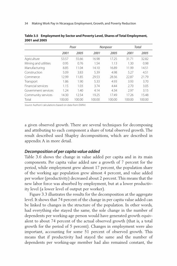
a given observed growth. There are several techniques for decomposingand attributing to each component a share of total observed growth. Theresult described used Shapley decompositions, which are described inappendix A in more detail.
Decomposition of per capita value addedTable 3.6 shows the change in value added per capita and in its maincomponents. Per capita value added saw a growth of 7 percent for theperiod, while employment grew almost 17 percent, the population shareof the working age population grew almost 4 percent, and value addedper worker (productivity) decreased about 2 percent.This means that thenew labor force was absorbed by employment, but at a lower productiv-ity level (a lower level of output per worker).
Figure 3.3 illustrates the results for the decomposition at the aggregatelevel. It shows that 74 percent of the change in per capita value added canbe linked to changes in the structure of the population. In other words,had everything else stayed the same, the sole change in the number ofdependents per working-age person would have generated growth equiv-alent to about 74 percent of the actual observed growth (that is, a totalgrowth for the period of 5 percent). Changes in employment were alsoimportant, accounting for some 51 percent of observed growth. Thismeans that if productivity had stayed the same and the number ofdependents per working-age member had also remained constant, the
34 Making Work Pay in Nicaragua: Employment, Growth, and Poverty Reduction
Table 3.5 Employment by Sector and Poverty Level, Shares of Total Employment,2001 and 2005
Poor Nonpoor Total
2001 2005 2001 2005 2001 2005
Agriculture 53.57 55.66 16.98 17.25 31.71 32.82Mining and utilities 0.95 0.76 1.54 1.13 1.30 0.98Manufacturing 8.85 11.04 14.10 16.89 11.99 14.51Construction 5.09 3.83 5.39 4.98 5.27 4.51Commerce 12.99 11.85 29.53 28.56 22.87 21.79Transport 1.86 1.90 5.33 4.93 3.93 3.70Financial services 1.15 1.03 3.74 4.44 2.70 3.05Government services 1.24 1.40 4.14 4.34 2.97 3.15Community services 14.30 12.54 19.25 17.49 17.26 15.48Total 100.00 100.00 100.00 100.00 100.00 100.00
Source: Authors’calculations based on data from EMNV.

higher rate of employment would have generated a growth of almost 4percent. Unfortunately, changes in productivity acted in the oppositedirection (–25.99 percent). Had productivity not changed, observedgrowth would have been 9 percent, but decreases in productivity meantthat growth was 1.6 percentage points lower.
Output, Population, Employment, and Poverty 35
Table 3.6 Percentage Change in Selected Variables, 2001–05
% Average annual change growth (%)
Value added 14.47 3.44Value added per capita 7.14 1.74Population 6.85 1.67Population of working age 12.47 2.98Employment 16.54 3.90Employment of working-age population 3.62 0.89Value added per worker –1.78 –0.45
Source: Authors’calculations based on data from BCN and EMNV.
share of working-age population
changes in share of working-age populationemployed
changes in outputper worker
74.35
51.64
–25.99
–40 –20 0 20 40 60 80
contribution to total change (%)
Figure 3.3 Aggregate Employment and Productivity Profile of Growth, 2001–05
Source: Authors’calculations based on data from BCN and EMNV.
Decomposition of changes in output per workerThe key question, then, is why did output per worker decrease? There aremany reasons why output per worker might have decreased. Workersmight have moved to a sector where marginal productivity is lower, totalfactor productivity (TFP) might have decreased, or the capital-to-laborratio may have been reduced as a result of the large inflow of workers intothe economy. These possible alternatives can be explored further bydecomposing the changes in aggregate output per worker into changesthat result from any of these three causes. Figure 3.4 shows the result ofthe decomposition of changes in output per worker for the aggregateeconomy. Total output per worker decreased 1.78 percent. Of thisdecrease, intersectoral employment shifts exerted a positive effect on out-put per worker (half a percentage point) or 6.72 percent of total produc-tivity growth. The capital-to-labor ratio also increased, contributing 1.68percentage points to output per worker; however, TFP suffered an impor-tant reduction, which explains 3.66 percentage points of the decrease inoutput per worker. These data clearly show that TFP changes are respon-sible for the decrease in output per worker.
To understand possible reasons for the observed decrease in TFP, it isimportant to understand that TFP was calculated as a residual (see appen-dix A), which means that it will capture all factors affecting output perworker other than capital and intersectoral shifts. Among the factors thatare likely to affect this residual in an important way are changes in theaverage skill of the labor force, which comprises both experience and edu-cation, and changes in the structure of employment by employment cat-egories (rather than by sectors). Reductions in the skills of the labor forcewould be reflected in lower TFP. Changes in the structure of employ-ment—characterized by increases in the number of workers employed inlow-productivity categories—will also be reflected in lower TFP. Forexample, if an important increase of total employment is concentratedamong family enterprises or the self-employed, which have lower-than-average productivity, then TFP will decrease.
As pointed out in chapter 2 (see table 2.5), the average years of edu-cation of the labor force increased, so the explanation for TFP decreasesdoes not lie on the level of education (at least if quality did not change).Tables 2.3 and 2.4 showed that employment had increased disproportion-ately among household enterprise workers and the individual self-employed, which are the categories with lowest earnings. If householdenterprise workers and the individual self-employed are also those cate-
36 Making Work Pay in Nicaragua: Employment, Growth, and Poverty Reduction
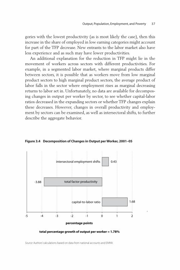
gories with the lowest productivity (as is most likely the case), then thisincrease in the share of employed in low earning categories might accountfor part of the TFP decrease. New entrants to the labor market also haveless experience and as such may have lower productivities.
An additional explanation for the reduction in TFP might lie in themovement of workers across sectors with different productivities. Forexample, in a segmented labor market, where marginal products differbetween sectors, it is possible that as workers move from low marginalproduct sectors to high marginal product sectors, the average product oflabor falls in the sector where employment rises as marginal decreasingreturns to labor set in. Unfortunately, no data are available for decompos-ing changes in output per worker by sector, to see whether capital-laborratios decreased in the expanding sectors or whether TFP changes explainthese decreases. However, changes in overall productivity and employ-ment by sectors can be examined, as well as intersectoral shifts, to furtherdescribe the aggregate behavior.
Output, Population, Employment, and Poverty 37
total factor productivity
capital-to-labor ratio 1.68
-3.88
0.43intersectoral employment shifts
-5 -4 -3 -2 -1 0 1 2
percentage points
total percentage growth of output per worker = 1.78%
Figure 3.4 Decomposition of Changes in Output per Worker, 2001–05
Source: Authors’calculations based on data from national accounts and EMNV.
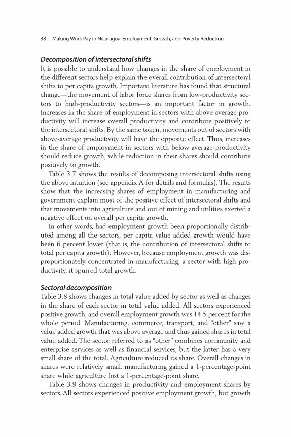
Decomposition of intersectoral shiftsIt is possible to understand how changes in the share of employment inthe different sectors help explain the overall contribution of intersectoralshifts to per capita growth. Important literature has found that structuralchange—the movement of labor force shares from low-productivity sec-tors to high-productivity sectors—is an important factor in growth.Increases in the share of employment in sectors with above-average pro-ductivity will increase overall productivity and contribute positively tothe intersectoral shifts. By the same token, movements out of sectors withabove-average productivity will have the opposite effect. Thus, increasesin the share of employment in sectors with below-average productivityshould reduce growth, while reduction in their shares should contributepositively to growth.
Table 3.7 shows the results of decomposing intersectoral shifts usingthe above intuition (see appendix A for details and formulas). The resultsshow that the increasing shares of employment in manufacturing andgovernment explain most of the positive effect of intersectoral shifts andthat movements into agriculture and out of mining and utilities exerted anegative effect on overall per capita growth.
In other words, had employment growth been proportionally distrib-uted among all the sectors, per capita value added growth would havebeen 6 percent lower (that is, the contribution of intersectoral shifts tototal per capita growth). However, because employment growth was dis-proportionately concentrated in manufacturing, a sector with high pro-ductivity, it spurred total growth.
Sectoral decompositionTable 3.8 shows changes in total value added by sector as well as changesin the share of each sector in total value added. All sectors experiencedpositive growth, and overall employment growth was 14.5 percent for thewhole period. Manufacturing, commerce, transport, and “other” saw avalue added growth that was above average and thus gained shares in totalvalue added. The sector referred to as “other” combines community andenterprise services as well as financial services, but the latter has a verysmall share of the total. Agriculture reduced its share. Overall changes inshares were relatively small: manufacturing gained a 1-percentage-pointshare while agriculture lost a 1-percentage-point share.
Table 3.9 shows changes in productivity and employment shares bysectors. All sectors experienced positive employment growth, but growth
38 Making Work Pay in Nicaragua: Employment, Growth, and Poverty Reduction
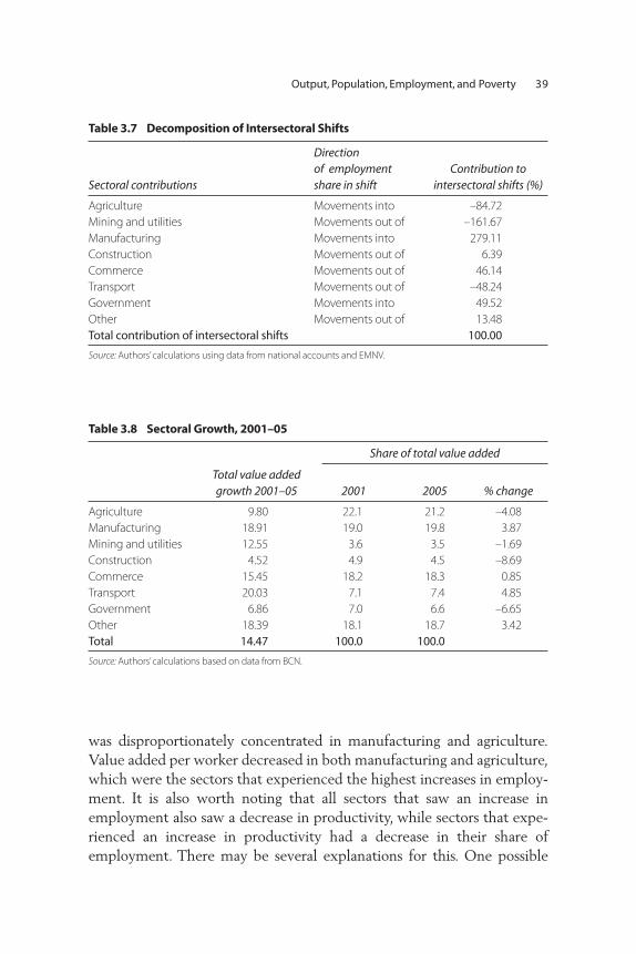
was disproportionately concentrated in manufacturing and agriculture.Value added per worker decreased in both manufacturing and agriculture,which were the sectors that experienced the highest increases in employ-ment. It is also worth noting that all sectors that saw an increase inemployment also saw a decrease in productivity, while sectors that expe-rienced an increase in productivity had a decrease in their share ofemployment. There may be several explanations for this. One possible
Output, Population, Employment, and Poverty 39
Table 3.7 Decomposition of Intersectoral Shifts
Direction of employment Contribution to
Sectoral contributions share in shift intersectoral shifts (%)
Agriculture Movements into –84.72Mining and utilities Movements out of –161.67Manufacturing Movements into 279.11Construction Movements out of 6.39Commerce Movements out of 46.14Transport Movements out of –48.24Government Movements into 49.52Other Movements out of 13.48Total contribution of intersectoral shifts 100.00
Source: Authors’calculations using data from national accounts and EMNV.
Table 3.8 Sectoral Growth, 2001–05
Share of total value added
Total value added growth 2001–05 2001 2005 % change
Agriculture 9.80 22.1 21.2 –4.08Manufacturing 18.91 19.0 19.8 3.87Mining and utilities 12.55 3.6 3.5 –1.69Construction 4.52 4.9 4.5 –8.69Commerce 15.45 18.2 18.3 0.85Transport 20.03 7.1 7.4 4.85Government 6.86 7.0 6.6 –6.65Other 18.39 18.1 18.7 3.42Total 14.47 100.0 100.0
Source: Authors’calculations based on data from BCN.

explanation is that changes in employment mainly capture new entrantsto the labor market and these new entrants have lower productivity thanmore experienced workers. The sectors that have a stronger increase inemployment growth absorb most of this new labor force and thus have astronger negative effect on average productivity. Alternatively, asexplained above, the inflow of workers into these sectors implied a lowercapital-labor ratio, as decreasing marginal returns to labor set.
Decreases in productivity and increases in employment were concen-trated in agriculture and manufacturing. Increases in the relative size ofthe manufacturing sector (in terms of employment) account for animportant share of growth. Table 3.10 illustrates the contribution of eachsector to total per capita value added growth for 2001–05. Sectoral con-tributions are decomposed into the (i) contribution of changes in outputper worker, (ii) contribution of the sector to employment rate growth,and (iii) contribution of the sector to the intersectoral shift component oftotal changes in output per worker (see appendix A for details). Overall,manufacturing, commerce, transport, and other services contributed pos-itively to growth, while agriculture, mining and utilities, construction, andgovernment had a negative contribution.
Despite the enormous employment growth in manufacturing, thedecrease in output per worker was so large that it more than offset the
Table 3.9 Employment Shares and Productivity, by Sectors of Economic Activity,2001–05
Absolute 2001 2005 % change 2001 2005 change
Agriculture 10,973 9,988 –8.97 19.21 20.60 1.39Manufacturing 25,032 21,097 –15.72 7.26 9.11 1.85Mining and utilities 43,097 55,364 28.47 0.79 0.62 –0.17Construction 14,701 15,393 4.70 3.19 2.83 –0.36Commerce 12,505 13,005 4.00 13.86 13.68 –0.18Transport 28,418 31,084 9.38 2.38 2.32 –0.06Government 37,223 32,239 –13.39 1.80 1.98 0.17Other 14,308 15,643 9.33 12.09 11.64 –0.45Total 15,757 15,477 –1.78 60.59 62.78 2.19
Source: Authors’calculations based on data from BCN and EMNV.
40 Making Work Pay in Nicaragua: Employment, Growth, and Poverty Reduction
Employment/working-age population (%)Output per worker (1994 C$)
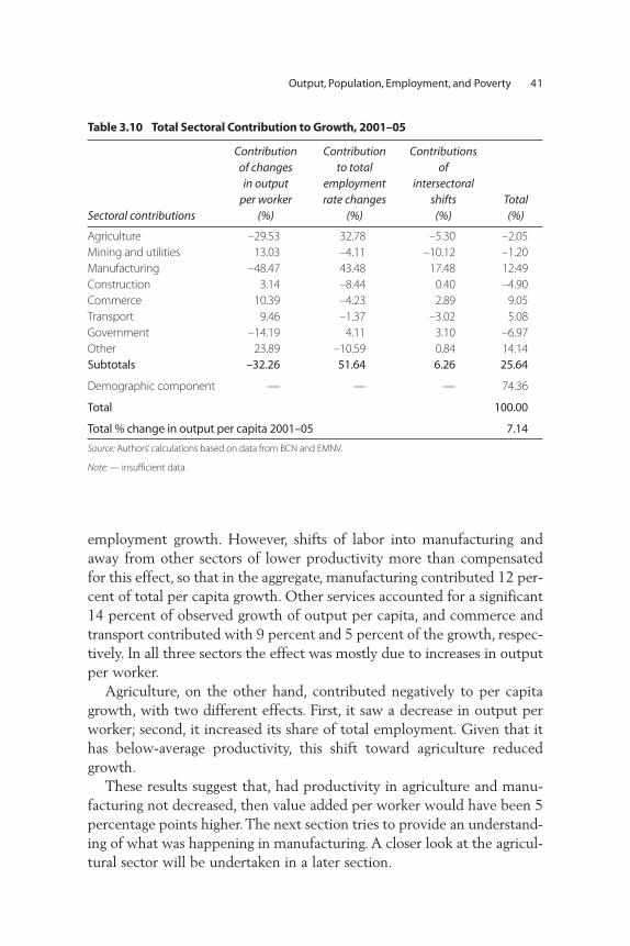
employment growth. However, shifts of labor into manufacturing andaway from other sectors of lower productivity more than compensatedfor this effect, so that in the aggregate, manufacturing contributed 12 per-cent of total per capita growth. Other services accounted for a significant14 percent of observed growth of output per capita, and commerce andtransport contributed with 9 percent and 5 percent of the growth, respec-tively. In all three sectors the effect was mostly due to increases in outputper worker.
Agriculture, on the other hand, contributed negatively to per capitagrowth, with two different effects. First, it saw a decrease in output perworker; second, it increased its share of total employment. Given that ithas below-average productivity, this shift toward agriculture reducedgrowth.
These results suggest that, had productivity in agriculture and manu-facturing not decreased, then value added per worker would have been 5percentage points higher.The next section tries to provide an understand-ing of what was happening in manufacturing. A closer look at the agricul-tural sector will be undertaken in a later section.
Table 3.10 Total Sectoral Contribution to Growth, 2001–05
Contribution Contribution Contributions of changes to total of in output employment intersectoral
per worker rate changes shifts Total Sectoral contributions (%) (%) (%) (%)
Agriculture –29.53 32.78 –5.30 –2.05Mining and utilities 13.03 –4.11 –10.12 –1.20Manufacturing –48.47 43.48 17.48 12.49Construction 3.14 –8.44 0.40 –4.90Commerce 10.39 –4.23 2.89 9.05Transport 9.46 –1.37 –3.02 5.08Government –14.19 4.11 3.10 –6.97Other 23.89 –10.59 0.84 14.14Subtotals –32.26 51.64 6.26 25.64
Demographic component — — — 74.36
Total 100.00
Total % change in output per capita 2001–05 7.14
Source: Authors’calculations based on data from BCN and EMNV.
Note: — insufficient data.
Output, Population, Employment, and Poverty 41

The behavior of wagesThe effects of changes in employment and productivty on povertydepend on how they affect earnings. Table 3.11 presents the medianwages by sector of economic activity, calculated from the household sur-veys.The table shows that, in real terms, wages in agriculture increased 17percent while wages in manufacturing decreased 2 percent between 2001and 2005. As will be seen, lower value added per worker in agriculturewas compensated by higher producer prices, which may have preventedthe falls in productivity from translating into lower wages. In the case ofthe manufacturing sector, wages did decrease, but much less than produc-tivity, so that productivity falls were not totally passed on to wages.
A Closer Look at the Manufacturing Sector
Table 3.12 shows employment generation by subsector. In an analysis ofwhich sectors absorbed most of the employment generation, 66 percentof the employment growth was in the food and beverage sector and theclothing sector. The tobacco sector contributed to an additional 8 percentof employment generation. The last row of the table shows employmentgeneration by maquila, which contributed an amazing 32 percent ofemployment generation between 2001 and 2005, most of which wasclothing (see box 3.1).
Table 3.13 shows the median wages for these sectors. The two sectorsthat generated most of the employment growth in manufacturing (food
Table 3.11 Wages by Sector of Economic Activity, 2001 and 2005
Median wage C$ 2001
2001 2005 Real growth (%)
Agriculture 6,840 8,018 17.2Mining and utilities 20,000 23,495 17.5Manufacturing 12,600 12,364 –1.9Construction 10,080 10,000 –0.8Commerce 13,329 13,364 0.3Transport 18,900 18,327 –3.0Financial services 18,175 21,238 16.9Government services 23,665 25,833 9.2Community services 12,179 14,118 15.9
Source: Authors’calculations based on data from EMNV.
42 Making Work Pay in Nicaragua: Employment, Growth, and Poverty Reduction

and clothing) saw differing behavior. In the food sector, median wagesdecreased, while wages in the clothing sector increased.
Another way of looking at the types of jobs generated is to see whichtype of employment showed more growth. In Nicaragua the lowestincome is observed in those working in household family enterprises, fol-lowed by the individual self-employed, while the highest income corre-sponds to employers, followed by waged and salaried workers. Table 3.14shows that 32 percent of the employment generated in manufacturingwas concentrated in family enterprise workers, 17 percent was in the indi-vidual self-employed, and 55 percent was in the waged and salaried cate-gories. This means that 48 percent of the jobs created in manufacturingwere low income.
It is worth noting that the maquila sector may have played an impor-tant role in counteracting the negative effect of the growing number ofemployed in family enterprises and the decreasing wages in the food
Output, Population, Employment, and Poverty 43
Table 3.12 Employment Generation by Subsector, 2001 and 2005
Employment Share of growth Employment total
Total number (number of growth employment of employed new jobs) (%) generation
2001 2005 2001–05 2001–05 2001–05
Food and beverage 69,754 100,398 30,644 43.93 38.54Tobacco 1,118 7,394 6,276 561.35 7.89Textiles 4,305 6,472 2,167 50.34 2.73Clothing 62,811 84,989 22,178 35.31 27.89Wood products 8,766 10,571 1,805 20.59 2.27Paper and prints 2,455 5,210 2,755 112.25 3.47Petroleum 469 622 153 32.52 0.19Chemicals 1,752 2,926 1,174 67.02 1.48Plastic and rubber 1,441 1,362 –79 –5.46 –0.10Other nonmetallic mineral 10,917 13,461 2,544 23.31 3.20
productsMetal and metal products 14,597 16,460 1,864 12.77 2.34Machinery and equipment 1,945 3,695 1,750 89.99 2.20Transport equipment 443 634 190 42.96 0.24Other 15,271 21,355 6,084 39.84 7.65Total manufacturing 196,043 275,549 79,506 40.56 100.00
Maquila employment 35,565 61,000 25,435 71.52 31.99
Source: Authors’calculations based on data from EMNV.
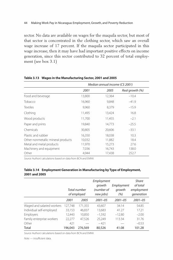
sector. No data are available on wages for the maquila sector, but most ofthat sector is concentrated in the clothing sector, which saw an overallwage increase of 17 percent. If the maquila sector participated in thiswage increase, then it may have had important positive effects on incomegeneration, since this sector contributed to 32 percent of total employ-ment (see box 3.1)
44 Making Work Pay in Nicaragua: Employment, Growth, and Poverty Reduction
Table 3.13 Wages in the Manufacturing Sector, 2001 and 2005
Median annual income (C$ 2001)
2001 2005 Real growth (%)
Food and beverage 13,800 12,364 –10.4
Tobacco 16,960 9,848 –41.9
Textiles 9,960 8,379 –15.9
Clothing 11,495 13,424 16.8
Wood products 11,700 11,455 –2.1
Paper and prints 19,840 14,773 –25.5
Chemicals 30,805 20,606 –33.1
Plastic and rubber 16,350 18,038 10.3Other nonmetallic mineral products 10,032 11,882 18.4Metal and metal products 11,970 15,273 27.6Machinery and equipment 7,036 16,743 138.0Other 4,944 17,438 252.7
Source: Authors’calculations based on data from BCN and EMNV.
Table 3.14 Employment Generation in Manufacturing by Type of Employment, 2001 and 2005
Employment Share growth Employment of total
Total number (number of growth employment of employed new jobs) (%) generation
2001 2005 2001–05 2001–05 2001–05
Waged and salaried workers 127,748 171,355 43,607 34.14 54.85Individual self-employed 33,153 46,837 13,683 41.27 17.21Employers 12,443 10,850 –1,592 –12.80 –2.00 Family enterprise workers 22,277 47,526 25,249 113.34 31.76Other 421 — – 421 — –0.53Total 196,043 276,569 80,526 41.08 101.28
Source: Authors’calculations based on data from BCN and EMNV.
Note: — insufficient data.
Output, Population, Employment, and Poverty 45
The main picture that emerges from this chapter is as follows. Growthwas mainly concentrated in the manufacturing sector. Employmentgrowth was concentrated in both manufacturing and agriculture.Unfortunately, this growth had a limited impact on the income opportu-nities of the poor. On the one hand, despite the fact that wages in agri-culture increased, returns in this sector still offer the lowest income gen-eration, so that growing employment in this sector is not likely to reducepoverty. On the other hand, employment generated in manufacturing wasdivided evenly between family enterprise employment and wage employ-ment. Family enterprise employment has a very low income-generationpotential. Wage employment has a better potential, but its benefits to thepoor seem to have been limited by two main factors: (i) wages decreasedin the food sector, which saw most of the employment growth in manu-facturing; and (ii) clothing, which was the other important sector in terms
Box 3.1
Evolution of the Maquila Sector and Its Importance in the Employment Growth in Manufacturing
The first maquila factories started in 1990, with the establishment of the first pub-
licly owned export processing zone (EPZ), Las Mercedes. In 1994 the EPZ law was
reformed to allow private ownership by both foreign and domestic investors and
an expansion of EPZ to other regions in the country, with the particular aim of
providing employment opportunities for poorer areas. Currently, there is the
zone of Las Mercedes. The rest are distributed in 30 industrial parks, which are pri-
vate EPZs. The main investors are from Taiwan, the United States, the Republic of
Korea, Nicaragua, Italy, Honduras, Belize, and Mexico.
Initially, EPZ firms were not allowed to use domestic raw materials, which lim-
ited their spillover effects to those of employment generation, but with the sign-
ing of the Central American Free Trade Agreement, these restrictions were re-
moved. EPZs have a 100 percent exemption on corporate income tax for the first
15 years of operation. They are exempt from capital gains on real estate; all cor-
porate taxes; excise, sales, and municipal taxes; and import duties on machinery,
inputs, and equipment. Currently there are 84 firms, of which the large majority
are in the clothing sector.
(continued)
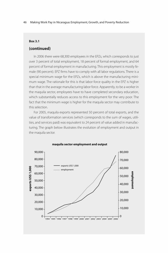
46 Making Work Pay in Nicaragua: Employment, Growth, and Poverty Reduction
Box 3.1
(continued)
In 2006 there were 68,300 employees in the EPZs, which corresponds to just
over 3 percent of total employment, 18 percent of formal employment, and 64
percent of formal employment in manufacturing. This employment is mostly fe-
male (90 percent). EPZ firms have to comply with all labor regulations. There is a
special minimum wage for the EPZs, which is above the manufacturing mini-
mum wage. The rationale for this is that labor force quality in the EPZ is higher
than that in the average manufacturing labor force. Apparently, to be a worker in
the maquila sector, employees have to have completed secondary education,
which substantially reduces access to this employment for the very poor. The
fact that the minimum wage is higher for the maquila sector may contribute to
this selection.
For 2005, maquila exports represented 50 percent of total exports, and the
value of transformation services (which corresponds to the sum of wages, utili-
ties, and services paid) was equivalent to 24 percent of value added in manufac-
turing. The graph below illustrates the evolution of employment and output in
the maquila sector.
exp
ort
s U
S$ 1
,00
0
emp
loym
ent
90,000
80,000
70,000
60,000
50,000
40,000
30,000
20,000
10,000
0
80,000
70,000
60,000
50,000
40,000
30,000
20,000
10,000
0
maquila sector employment and output
1994 1998199719961995 1999 2000 20052004200320022001 2006
exports US$ 1,000
employment
of job creation, offered limited employment access for the poor becauseof its skill requirements (secondary education or above).
Notes
1. This increase is net of those ages 60–64 who will be exiting the labor market.
2. The Household Survey for 2001 (EMNV 2001) shows a rural share of thepopulation that is inconsistent with the census. According to the survey, theshare of rural population increased between 2001 and 2005.The census showsthe opposite. Apparently the survey of 2001 underestimated the rural popula-tion. If this is the case, the increase in the share of employed in agriculturemight be exclusively due to the under-representation of rural households inthe survey of 2001.
Output, Population, Employment, and Poverty 47
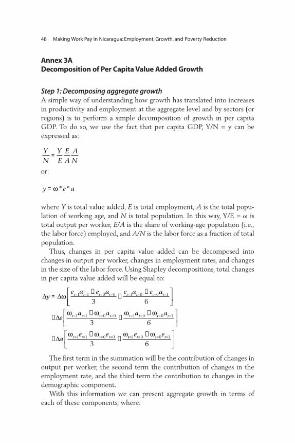
Annex 3ADecomposition of Per Capita Value Added Growth
Step 1: Decomposing aggregate growthA simple way of understanding how growth has translated into increasesin productivity and employment at the aggregate level and by sectors (orregions) is to perform a simple decomposition of growth in per capitaGDP. To do so, we use the fact that per capita GDP, Y/N = y can beexpressed as:
or:
where Y is total value added, E is total employment, A is the total popu-lation of working age, and N is total population. In this way, Y/E = istotal output per worker, E/A is the share of working-age population (i.e.,the labor force) employed, and A/N is the labor force as a fraction of totalpopulation.
Thus, changes in per capita value added can be decomposed intochanges in output per worker, changes in employment rates, and changesin the size of the labor force. Using Shapley decompositions, total changesin per capita value added will be equal to:
The first term in the summation will be the contribution of changes inoutput per worker, the second term the contribution of changes in theemployment rate, and the third term the contribution to changes in thedemographic component.
With this information we can present aggregate growth in terms ofeach of these components, where:
48 Making Work Pay in Nicaragua: Employment, Growth, and Poverty Reduction
YN
YE
EA
AN
=
y e a= ω * *
∆ ∆ye a e a e a e at t t t t t t t=
++
+⎡ = = = = = = = =ω 1 1 0 0 1 0 0 1
3 6⎣⎣⎢
⎤
⎦⎥
++
++= = = = = =∆e
a a at t t t t tω ω ω ω1 1 0 0 1 0
3tt t
t t t t
a
ae e
= =
= = = =
⎡
⎣⎢
⎤
⎦⎥
++
+
0 1
1 1 0 0
6
3∆
ω ω ω tt t t te e= = = =+⎡
⎣⎢
⎤
⎦⎥
1 0 0 1
6ω
will be the fraction of growth that can be linked to changes in output perworker,
will be the fraction of growth that can be linked to changes in theemployment rate, and
will be the fraction of growth that can be linked to changes in the shareof total population that is of working age, and where the bar denotes thefraction of growth explained by the component. In this way percentagegrowth between two periods can be expressed as follows:
Once we have decomposed aggregate employment growth we can gofurther and understand, first, the role played by different sectors inchanges in employment, and second, the role of capital, total factor pro-ductivity (TFP), and intersectoral shifts in explaining changes in outputper worker, both at the aggregate level and by sectors. This amounts todoing a stepwise decomposition, first decomposing aggregate growth intoemployment and productivity changes, and then decomposing employ-ment and productivity changes by sectors.
Step 2: Understanding which sectors contributed most to employment generationTo understand which sectors contributed to most of the employmentgeneration, we can further decompose employment growth (e) by sec-tors. The easiest is of course to express the total growth in employmentas the sum of employment generation in each sector, as follows:
Output, Population, Employment, and Poverty 49
ω ω≡+
++⎡
⎣= = = = = = = =∆
e a e a e a e at t t t t t t t1 1 0 0 1 0 0 1
3 6⎢⎢⎤
⎦⎥ / ∆y
e ea a a at t t t t t t t≡
++
+⎡
⎣= = = = = = = =∆
ω ω ω ω1 1 0 0 1 0 0 1
3 6⎢⎢⎤
⎦⎥ / ∆y
a ae e e et t t t t t t t≡
++
+⎡
⎣= = = = = = = =∆
ω ω ω ω1 1 0 0 1 0 0 1
3 6⎢⎢⎤
⎦⎥ / ∆y
∆ ∆ ∆ ∆yy
yy
eyy
ayy
= + +ω
∆ ∆e eii
s
==∑
1
where
is just the change in employment in sector i as a share of total working-age population. Let
denote the fraction of the aggregate employment rate change that can belinked to changes in employment in sector i. The supraindex e will makeexplicit that it is the contribution to employment growth (as opposed tototal per capita growth).
Step 3: Decomposing changes in output per worker by sectors and between and within componentsWe can further decompose output per worker into sectoral employmentshifts and changes in output per worker by sectors by noting that:
or equivalently:
where Yi is value added of sector i = 1…S, Ei is employment in sector i,and E is total employment. This means that
will correspond to output per worker in sector i, and
is the share of sector i in total employment. This equation just states thatchanges in output per worker are the weighted sum of changes in outputper worker in all sectors, where the weights are simply the employmentshare of each sector.
50 Making Work Pay in Nicaragua: Employment, Growth, and Poverty Reduction
∆ ∆eEAi
i=
e e ei
ei≡∆ ∆/
sEEi
i=
ω ii
i
YE
=
ω ω==∑ i ii
S
s1
YE
YE
EE
i
iS
i= ∑
Using the Shapley approach, changes in aggregate output per workercan be decomposed as:
Each term
is the change in output per worker that can be linked to changes in out-put per worker in sector s. The last term in the equation, B, is thechange in output per worker due to intersectoral employment changes(i.e., between sectors). That is, employment movement from low-pro-ductivity sectors to high-productivity sectors should increase total out-put per worker, and the flows from high-productivity sectors to low-pro-ductivity sectors should reduce aggregate output per worker. If this lastterm is negative, the reallocation of employment by sectors was detri-mental to overall productivity growth. Finally, the term W correspondsto total changes in output per worker net of relocation effects (this com-ponent is also referred to as the “within” component in the decomposi-tion literature).
We can then denote the fraction of aggregate output per workergrowth that can be linked to growth in output per worker in sector i as
where again the bar denotes the fact that we are referring to contribu-tions, and the supraindex denotes the fact that it is a contribution toaggregate output per worker growth , rather than a contribution to out-put per capita growth y.
Output, Population, Employment, and Poverty 51
∆ ∆ ∆ω ω ω=+⎛
⎝⎜⎞
⎠⎟+
+= = =1
1 0 1 12
2 0 2
2* *, , , ,s s s st t t t == = =⎛
⎝⎜⎞
⎠⎟+ +
+⎛
⎝⎜⎞
⎠⎟1 0 1
2 2... * , ,∆
∆
ω
ω
ii t i ts s
w
* ,+ ∆siiω tt i t
i
S
B
= =
=
+⎛
⎝⎜⎞
⎠⎟∑ 0 1
1 2
ω
ω
,
∆
∆ω ii t i ts s
* , ,= =+⎛
⎝⎜⎞
⎠⎟0 1
2
ω ω ωωi i
i t i ts s≡
+⎛
⎝⎜⎞
⎠⎟= =∆ ∆* /, ,0 1
2
Similarly, we can define the contribution of within-sector productivitygrowth as
and the contribution of intersectoral shifts as
Step 4: Understanding the sources of changes in output per worker(net of intersectoral shifts) at the aggregate level and by sectorsThe terms and i will capture changes in output per worker, but theirinterpretation is not so straightforward. Increases in output per workercan come from three different sources: (i) increases in the capital-laborratio, (ii) increases in TFP, and (iii) relocation of jobs from bad jobs sec-tors (low productivity) to good jobs sectors (high productivity). To seethe first two sources, note that under constant returns to scale, ifYt=t f (Et,Kt), where Kt is the capital stock and t is a technologicalparameter also know as total factor productivity, then output per workercan be expressed as Yt/Et=t f (l, Kt/Et). Therefore, output per worker,Yt/Et, will depend on changes in capital-labor ratio and in TFP growth.Note that it may also capture cyclical behavior of output: firms operatingin economic downturns may have underutilized capital, so when thedemand rises again it will be reflected as rise in output per worker. Thethird source is simply the result of workers moving from a low-produc-tivity sector (or firm) to a high-productivity sector (or firm), so that in theaggregate, average output per worker will rise. From step 3 we found thatit is possible to isolate the effect of intersectoral shifts. The term w isjust changes in output per worker net of intersectoral shifts.
If data on capital stock are available, then we can assume a particularfunctional form for the production function and separate the contribu-tion of higher capital-labor ratios and TFP. For example, if we are willingto assume that the production function is Cobb-Douglas, then:
52 Making Work Pay in Nicaragua: Employment, Growth, and Poverty Reduction
YE
KE
= ⎛⎝⎜
⎞⎠⎟
−
Φ1 α
ω ω ωωB B≡∆ ∆/
ω ω ωωw w≡∆ ∆/
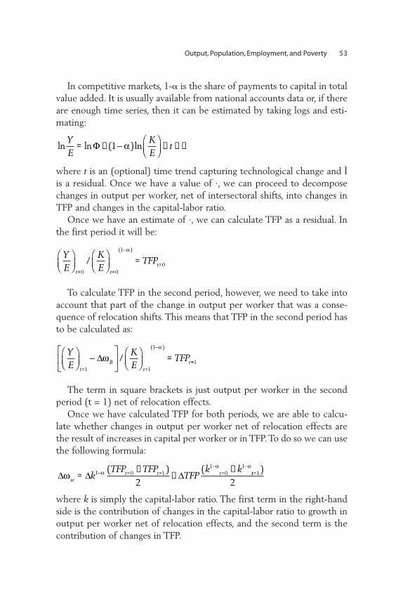
In competitive markets, 1- is the share of payments to capital in totalvalue added. It is usually available from national accounts data or, if thereare enough time series, then it can be estimated by taking logs and esti-mating:
where t is an (optional) time trend capturing technological change and Ìis a residual. Once we have a value of ·, we can proceed to decomposechanges in output per worker, net of intersectoral shifts, into changes inTFP and changes in the capital-labor ratio.
Once we have an estimate of ·, we can calculate TFP as a residual. Inthe first period it will be:
To calculate TFP in the second period, however, we need to take intoaccount that part of the change in output per worker that was a conse-quence of relocation shifts. This means that TFP in the second period hasto be calculated as:
The term in square brackets is just output per worker in the secondperiod (t = 1) net of relocation effects.
Once we have calculated TFP for both periods, we are able to calcu-late whether changes in output per worker net of relocation effects arethe result of increases in capital per worker or in TFP. To do so we can usethe following formula:
where k is simply the capital-labor ratio. The first term in the right-handside is the contribution of changes in the capital-labor ratio to growth inoutput per worker net of relocation effects, and the second term is thecontribution of changes in TFP.
Output, Population, Employment, and Poverty 53
YE
KE
TFPt t
t
⎛⎝⎜
⎞⎠⎟
⎛⎝⎜
⎞⎠⎟
== =
−
=0 0
1
0/( )α
YE
KE
TFPt
Bt
t
⎛⎝⎜
⎞⎠⎟
−⎡
⎣⎢
⎤
⎦⎥
⎛⎝⎜
⎞⎠⎟
== =
−
1 1
1
∆ωα
/( )
==1
∆ ∆ ∆ω αα α
wt t tk
TFP TFPTFP
k k=
++
+− = =−
=−
1 0 11
01
2( ) ( tt =1
2)
ln ln ( )lnYE
KE
t= + − ⎛⎝⎜
⎞⎠⎟
+ +Φ 1 α µ
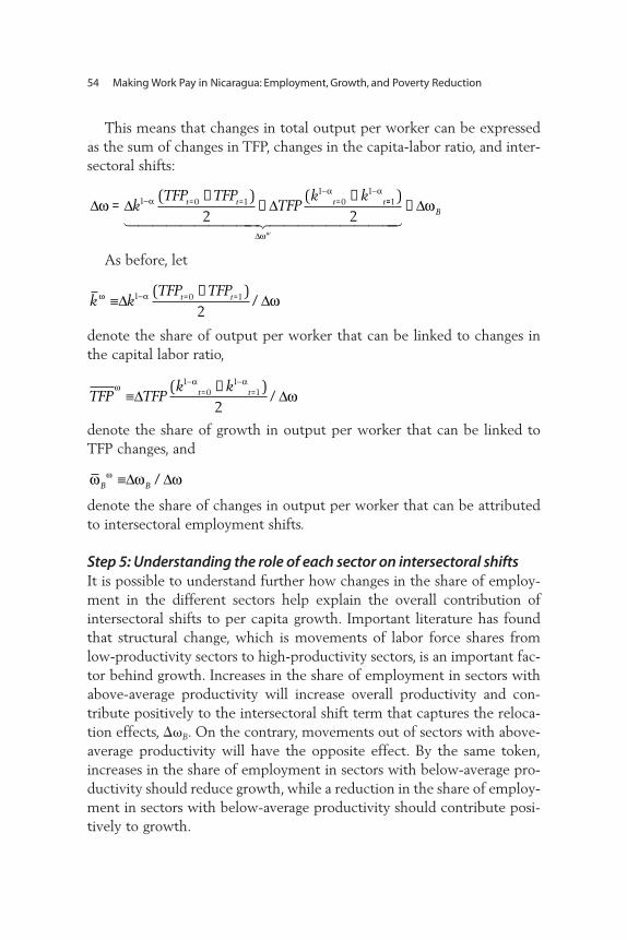
This means that changes in total output per worker can be expressedas the sum of changes in TFP, changes in the capita-labor ratio, and inter-sectoral shifts:
As before, let
denote the share of output per worker that can be linked to changes inthe capital labor ratio,
denote the share of growth in output per worker that can be linked toTFP changes, and
denote the share of changes in output per worker that can be attributedto intersectoral employment shifts.
Step 5: Understanding the role of each sector on intersectoral shiftsIt is possible to understand further how changes in the share of employ-ment in the different sectors help explain the overall contribution ofintersectoral shifts to per capita growth. Important literature has foundthat structural change, which is movements of labor force shares fromlow-productivity sectors to high-productivity sectors, is an important fac-tor behind growth. Increases in the share of employment in sectors withabove-average productivity will increase overall productivity and con-tribute positively to the intersectoral shift term that captures the reloca-tion effects, B. On the contrary, movements out of sectors with above-average productivity will have the opposite effect. By the same token,increases in the share of employment in sectors with below-average pro-ductivity should reduce growth, while a reduction in the share of employ-ment in sectors with below-average productivity should contribute posi-tively to growth.
54 Making Work Pay in Nicaragua: Employment, Growth, and Poverty Reduction
∆ ∆ ∆ω αα α
=+
++− = =
−=
−
kTFP TFP
TFPk kt t t t1 0 1
10
1
2( ) ( == +1
2)
∆
∆
ω
ω
w
B
ω ω ωωB B≡∆ ∆/
k kTFP TFPt tω α ω≡
+− = =∆ ∆1 0 1
2( )
/
TFP TFPk kt t
ωα α
ω≡+−
=−
=∆ ∆( )
/1
01
1
2
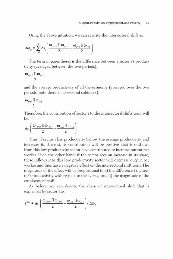
Using the above intuition, we can rewrite the intersectoral shift as:
The term in parentheses is the difference between a sector i’s produc-tivity (averaged between the two periods),
and the average productivity of all the economy (averaged over the twoperiods; note there is no sectoral subindex),
Therefore, the contribution of sector i to the intersectoral shifts term willbe:
Thus, if sector i has productivity bellow the average productivity, andincreases its share si, its contribution will be positive, that is outflowsfrom this low productivity sector have contributed to increase output perworker. If on the other hand, if the sector sees an increase in its share,these inflows into this low productivity sector will decrease output perworker and thus have a negative effect on the intersectoral shift term.Themagnitude of the effect will be proportional to: i) the difference I the sec-tor’s productivity with respect to the average and ii) the magnitude of theemployment shift.
As before, we can denote the share of intersectoral shift that isexplained by sector i as:
Output, Population, Employment, and Poverty 55
∆ ∆ωω ω ω ω
B ii t i t t t
i
S
s=+
−+⎛
⎝⎜⎞
⎠⎟= = = =
=∑ , ,0 1 0 1
1 2 2
ω ωi t i t, ,= =+0 1
2
ω ωt t= =+0 1
2
∆sii t i t t t
ω ω ω ω, ,= = = =+
−+⎛
⎝⎜⎞
⎠⎟0 1 0 1
2 2
s si ii t i t t t
BBω ω ω ω ω
ω=+
−+⎛
⎝⎜⎞
⎠⎟= = = =∆ ∆, , /0 1 0 1
2 2
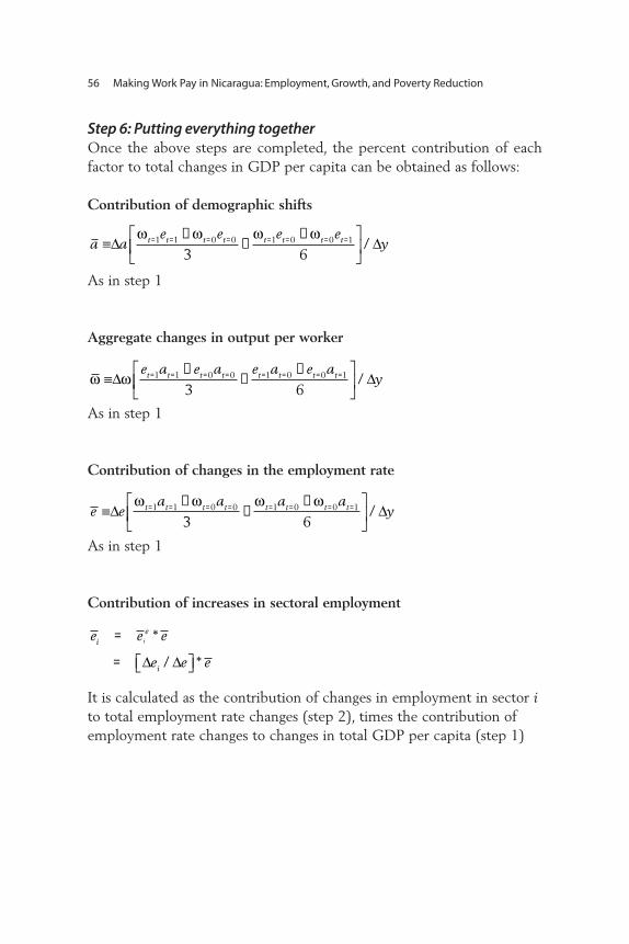
Step 6: Putting everything togetherOnce the above steps are completed, the percent contribution of eachfactor to total changes in GDP per capita can be obtained as follows:
Contribution of demographic shifts
As in step 1
Aggregate changes in output per worker
As in step 1
Contribution of changes in the employment rate
As in step 1
Contribution of increases in sectoral employment
It is calculated as the contribution of changes in employment in sector ito total employment rate changes (step 2), times the contribution ofemployment rate changes to changes in total GDP per capita (step 1)
56 Making Work Pay in Nicaragua: Employment, Growth, and Poverty Reduction
a ae e e et t t t t t t t≡
++
+⎡
⎣= = = = = = = =∆
ω ω ω ω1 1 0 0 1 0 0 1
3 6⎢⎢⎤
⎦⎥ / ∆y
ω ω≡+
++⎡
⎣= = = = = = = =∆
e a e a e a e at t t t t t t t1 1 0 0 1 0 0 1
3 6⎢⎢⎤
⎦⎥ / ∆y
e ea a a at t t t t t t t≡
++
+⎡
⎣= = = = = = = =∆
ω ω ω ω1 1 0 0 1 0 0 1
3 6⎢⎢⎤
⎦⎥ / ∆y
e e e
e e e
ie
i
i=
= ⎡⎣ ⎤⎦
*
/ *∆ ∆

Contribution of changes in output per worker within sectors
It is the contribution of within changes in output per worker to totalchanges in output per worker (step 3) times the contribution of aggre-gate output per worker to GDP per capita (step 1)
Contribution of intersectoral employment shifts
It is the contribution of between changes in output per worker to totalchanges in output per worker (step 3) times the contribution of aggre-gate output per worker to GDP per capita (step 1)
Within changes in output per worker in sector i
It is the contribution of sector i to within changes to total changes inoutput per worker (step 3) times the contribution of output per workerto changes in per capita GDP (step 1)
Output, Population, Employment, and Poverty 57
ω ω ω
ω
ωw w
ii t i t
i
S s s
=
=+⎛
⎝⎜⎞
⎠⎟⎛
⎝⎜
⎞
⎠= =
=∑
*
, ,*∆ 0 1
1 2 ⎟⎟⎡
⎣⎢⎢
⎤
⎦⎥⎥
/ *∆ω ω
ω ω ω
ω ωω
ωB B
ii t i t
i
S
s
=
=+⎛
⎝⎜⎞
⎠⎟⎡
⎣
= =
=∑
*
, ,* /∆ ∆0 1
1 2⎢⎢⎢
⎤
⎦⎥⎥*ω
ω ω ω
ω ω
ωi i
ii t i ts s
=
=+⎛
⎝⎜⎞
⎠⎟⎛
⎝⎜
⎞
⎠⎟
= =
*
* / *, ,∆ ∆0 1
2ωω
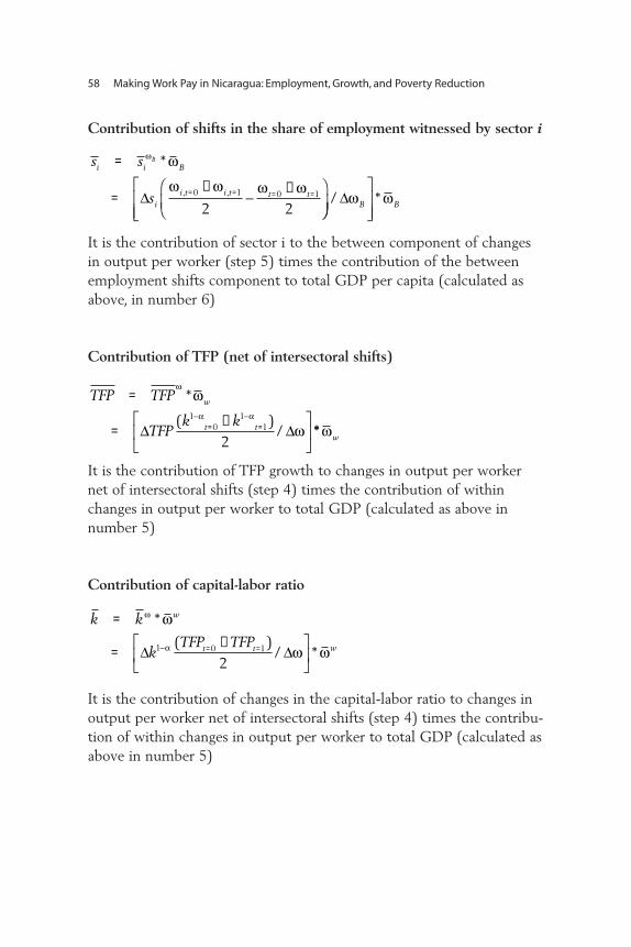
Contribution of shifts in the share of employment witnessed by sector i
It is the contribution of sector i to the between component of changesin output per worker (step 5) times the contribution of the betweenemployment shifts component to total GDP per capita (calculated asabove, in number 6)
Contribution of TFP (net of intersectoral shifts)
It is the contribution of TFP growth to changes in output per workernet of intersectoral shifts (step 4) times the contribution of withinchanges in output per worker to total GDP (calculated as above innumber 5)
Contribution of capital-labor ratio
It is the contribution of changes in the capital-labor ratio to changes inoutput per worker net of intersectoral shifts (step 4) times the contribu-tion of within changes in output per worker to total GDP (calculated asabove in number 5)
58 Making Work Pay in Nicaragua: Employment, Growth, and Poverty Reduction
k k
kTFP TFP
w
t t w
=
=+⎡
⎣⎢
⎤
⎦⎥
− = =
ω
α
ω
ω ω
*
( )/ *∆ ∆1 0 1
2
TFP TFP
TFPk k
w
t t
=
=+⎡
⎣⎢
⎤
⎦⎥
−=
−=
ω
α α
ω
ω
*
( )/∆ ∆
10
11
2**ωw
s s
s
i i B
ii t i t t t
B=
=+
−+⎛
⎝⎜⎞= = = =
ω ω
ω ω ω ω
*
, ,∆ 0 1 0 1
2 2 ⎠⎠⎟⎡
⎣⎢⎢
⎤
⎦⎥⎥
/ *∆ω ωB B
Some background knowledge of how labor income and its componentsaffect household poverty is useful to an understanding of what the prior-ity policies should be. A labor profile of the population should informpolicy makers as to how households are distributed among sectors, whattheir status in employment is, and what the determinants of per capitahousehold labor income are. This can be done by dividing the populationinto the poor and the nonpoor—defined according to national and inter-national poverty lines—or by using income quintiles. Another method forunderstanding how labor markets have affected household welfare is todisentangle the sources of labor income growth that are responsible forthe observed changes in total labor income.
This chapter is structured as follows: the first section sketches a laborprofile of the population; the second focuses on the decomposition ofhousehold labor income growth through the use of the panel componentof the 2001 and 2005 surveys; the final section is concerned with the agri-culture sector.
C H A P T E R 4
Employment and Labor IncomeProfile of the Population
59
Income and Employment Profile
Table 4.1 and table 4.2 show the employment status of the working-agepopulation by quintile and poverty level. There has been an increase intotal working-age population among the poor, which means that there arefewer dependent people within a household and there are potentiallybetter employment and income opportunities for the household as awhole. Among poor households, not all the members of working agelooked for a job (the inactive members increased from 39 percent in 2001to 40 percent in 2005), but most of those who sought a job actually foundone. The proportion of unemployed remained almost constant, while thenumber of employed increased by almost 1 percentage point.
The 2001 household survey asks the reasons for inactivity.Discouraged workers represent 11 percent among the poor and 8 percentamong the nonpoor. Those who are temporarily inactive (who have occa-sional jobs, are waiting for the harvest season, or are waiting to start a newjob) correspond to 3 percent of the inactive among the poor and 2 per-cent among the nonpoor. The largest shares of the inactive are homemak-ers and students: 52 percent and 34 percent are homemakers among thepoor and the nonpoor, respectively; 14 percent and 32 percent are study-ing (among the poor and nonpoor, respectively).
Benefits from formal employment among the poor and nonpoorTable 4.3 and table 4.4 describe the structure of employment by quintileand poverty level. The fraction employed in each category is shown as aproportion of employed individuals. As discussed above, wage employ-ment in the formal sector is very small; only 17 percent of the employedhave formal jobs, most of which are held by the nonpoor (14 percent).This close relationship between poverty and formal employment does nothave an immediate interpretation. Either poverty is a consequence of thelack of formal employment, or being poor hampers access to formalemployment. Alternatively, both informal employment and poverty maybe a consequence of lack of education and skills. It would be importantto look further into this relationship, to assess the importance of generat-ing formal employment in relation to removing barriers to employmentmobility among the poor, including access to education.
The number of wage workers employed in the informal sectordecreased by 7.8 percent. What is more important is that the decreasewas even greater among the poor than among the nonpoor (–13 percentcompared with –3.78 percent). The individual self-employed with no
60 Making Work Pay in Nicaragua: Employment, Growth, and Poverty Reduction
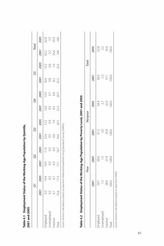
61
Tabl
e 4.
1Em
ploy
men
t Sta
tus o
f the
Wor
king
-Age
Pop
ulat
ion
by Q
uint
ile,
2001
and
200
5
Q1
Q2
Q3
Q4
Q5
Tota
l
2001
2005
2001
2005
2001
2005
2001
2005
2001
2005
2001
2005
Empl
oyed
9.3
10.4
10.4
11.6
12.4
12.2
13.6
13.4
16.4
15.2
62.2
62.8
Une
mpl
oyed
0.2
0.2
0.2
0.3
0.5
0.4
0.5
0.7
0.8
0.6
2.2
2.2
Inac
tive
6.1
6.7
6.5
6.9
6.6
7.4
8.2
6.6
8.2
7.4
35.6
35.0
Tota
l15
.617
.317
.118
.719
.620
.122
.320
.725
.523
.210
010
0
Sour
ce: A
utho
rs’c
alcu
latio
ns b
ased
on
data
from
Nat
iona
l Hou
seho
ld L
ivin
g St
anda
rds
Surv
ey (E
MN
V).
Tabl
e 4.
2Em
ploy
men
t Sta
tus o
f the
Wor
king
-Age
Pop
ulat
ion
by P
over
ty L
evel
, 200
1 an
d 20
05
Poor
Non
poor
Tota
l
2001
2005
2001
2005
2001
2005
Empl
oyed
59.7
60.6
61.2
64.4
60.6
62.8
Une
mpl
oyed
1.3
1.5
3.0
2.7
2.3
2.2
Inac
tive
38.9
37.9
35.8
32.9
37.1
35.0
Tota
l10
0.0
100.
010
0.0
100.
010
0.0
100.
0
Sour
ce: A
utho
rs’c
alcu
latio
ns b
ased
on
data
from
EM
NV.
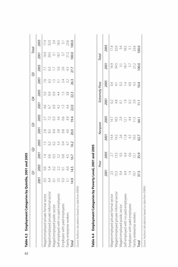
Tabl
e 4.
3Em
ploy
men
t Cat
egor
ies b
y Q
uint
ile, 2
001
and
2005
Q1
Q2
Q3
Q4
Q5
Tota
l
2001
2005
2001
2005
2001
2005
2001
2005
2001
2005
2001
2005
Wag
ed e
mpl
oyed
priv
ate
form
al s
ecto
r0.
50.
61.
41.
52.
82.
74.
65.
07.
67.
716
.917
.4W
aged
em
ploy
ed p
rivat
e in
form
al s
ecto
r6.
45.
46.
66.
28.
27.
26.
76.
96.
56.
334
.532
.0W
aged
em
ploy
ed p
ublic
sec
tor
0.1
0.2
0.3
0.2
0.4
0.3
0.9
0.9
1.5
1.7
3.1
3.4
Self-
empl
oyed
with
no
paid
em
ploy
ees
2.5
2.2
3.2
3.3
3.8
3.6
4.2
4.4
5.1
5.0
18.7
18.5
Empl
oyer
s w
ith p
aid
empl
oyee
s0.
30.
10.
80.
40.
80.
61.
31.
32.
42.
65.
75.
1Fa
mily
ent
erpr
ise w
orke
rs5.
16.
04.
54.
74.
04.
94.
43.
83.
24.
321
.223
.6To
tal
14.9
14.5
16.7
16.2
20.0
19.4
22.0
22.3
26.3
27.7
100.
010
0.0
Sour
ce: A
utho
rs’c
alcu
latio
ns b
ased
on
data
from
EM
NV.
Tabl
e 4.
4Em
ploy
men
t Cat
egor
ies b
y Po
vert
y Le
vel,
2001
and
200
5
Poor
Non
poor
Extr
emel
y Po
orTo
tal
2001
2005
2001
2005
2001
2005
2001
2005
Wag
ed e
mpl
oyed
priv
ate
form
al s
ecto
r2.
52.
714
.414
.70.
20.
416
.917
.4W
aged
em
ploy
ed p
rivat
e in
form
al s
ecto
r15
.313
.519
.218
.54.
84.
134
.532
.0W
aged
em
ploy
ed p
ublic
sec
tor
0.4
0.5
2.6
2.9
0.1
0.2
3.1
3.4
Self-
empl
oyed
with
no
paid
em
ploy
ees
6.9
6.4
11.8
12.1
1.9
1.4
18.7
18.5
Empl
oyer
s w
ith p
aid
empl
oyee
s1.
40.
64.
24.
40.
20.
05.
75.
1Fa
mily
ent
erpr
ise w
orke
rs10
.712
.110
.511
.53.
94.
321
.223
.6To
tal
37.3
35.9
62.7
64.1
11.1
10.4
100.
010
0.0
Sour
ce: A
utho
rs’c
alcu
latio
ns b
ased
on
data
from
EM
NV.
62

paid employees and also employers with paid employees decreased theirshare among the poor, while the number of family enterprises—oftenassociated with low income generation—rose by about 1 percentagepoint for both the poor and the nonpoor. The number of poor employedin the public sector remained almost constant.
Increases in public transfers and remittancesPublic transfers increased for the poor, while remittances increased forthe entire population (but less so for the poor). Table 4.5 and table 4.6show the earnings profile of the population by quintile and by povertylevel. No significant differences are evident in the income structure of thepopulation. For all levels of income, wage employment is the main sourceof income, accounting for a little over 45 percent of total income. Themain difference is that poor wage earners receive their earnings from agri-culture. This share decreased slightly for all income levels as remittancesand public transfers increased. Remittances for the nonpoor showed thelargest increase, while public transfers showed the greatest increase forthe poor, and among them, for the extremely poor. It is worth noting thatin 2001 public transfers were regressive in the sense that the poorreceived fewer transfers as a proportion of their total income. In 2005 thissituation changed and public transfers became progressive.
Decomposition of Changes in Labor Income
A traditional way to understand how labor markets have affected welfareis to disentangle the sources of household per capita labor income that areresponsible for observed growth or decreases in average householdincome.1 Per capita household labor income—that is, the total incomethat the household earns from labor divided by the number of membersin the household—can change for several reasons: because income peremployed member increases, because unemployment decreases, becausethe number of members that actively participate in the labor market rises,or because the dependency rate decreases.
This section discusses the main source of per capita labor incomegrowth between 2001 and 2005. The panel component of the survey isused to decompose, for each household, how much of the change in laborincome was attributed to changes in each of the components mentionedabove (see appendix B for the methodology). In addition, the method dif-ferentiates between four types of employment: wage work in agriculture,
Employment and Labor Income Profile of the Population 63
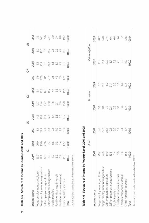
64
Tabl
e 4.
5St
ruct
ure
of In
com
e by
Qui
ntile
, 200
1 an
d 20
05
Q1
Q2
Q3
Q4
Q5
Inco
me
sour
ce20
0120
0520
0120
0520
0120
0520
0120
0520
0120
05
Wag
e em
ploy
men
t agr
icul
ture
29.2
26.0
15.1
14.5
12.7
9.1
5.9
5.5
3.0
3.3
Wag
e em
ploy
men
t non
agric
ultu
re18
.115
.029
.126
.735
.432
.337
.036
.740
.034
.1Se
lf-em
ploy
men
t agr
icul
ture
22.3
27.6
17.3
21.4
13.7
14.3
8.5
8.6
3.6
5.6
Self-
empl
oym
ent n
onag
ricul
ture
8.8
7.2
16.4
12.5
17.0
16.7
21.9
21.4
25.2
22.1
Publ
ic tr
ansf
ers
1.9
6.8
0.8
5.4
1.6
4.4
2.6
3.1
2.3
3.0
Fam
ily re
mitt
ance
s (in
tern
al)
3.6
3.3
4.0
3.3
2.1
3.5
4.3
3.9
2.6
3.4
Fam
ily re
mitt
ance
s (e
xter
nal)
0.9
1.4
1.3
2.6
2.6
4.2
2.6
4.9
4.4
8.8
Oth
er n
onla
bor s
ourc
es15
.312
.715
.913
.715
.015
.617
.115
.918
.919
.7To
tal
100.
010
0.0
100.
010
0.0
100.
010
0.0
100.
010
0.0
100.
010
0.0
Sour
ce: A
utho
rs’c
alcu
latio
ns b
ased
on
data
from
EM
NV.
Tabl
e 4.
6St
ruct
ure
of In
com
e by
Pov
erty
Lev
el, 2
001
and
2005
Poor
Non
poor
Extr
emel
y Po
or
Inco
me
sour
ce20
0120
0520
0120
0520
0120
05
Wag
e em
ploy
men
t agr
icul
ture
20.7
18.6
5.9
5.0
30.8
28.2
Wag
e em
ploy
men
t non
agr
icul
ture
24.6
22.2
38.6
35.1
16.4
14.0
Self-
empl
oym
ent a
gric
ultu
re19
.023
.27.
38.
222
.227
.4Se
lf-em
ploy
men
t non
agric
ultu
re13
.810
.522
.121
.18.
76.
4Pu
blic
tran
sfer
s1.
46.
02.
33.
21.
86.
6Fa
mily
rem
ittan
ces
(inte
rnal
)3.
63.
33.
13.
64.
03.
4Fa
mily
rem
ittan
ces
(ext
erna
l)1.
42.
43.
46.
40.
91.
2O
ther
non
labo
r sou
rces
15.6
13.7
17.4
17.5
15.2
12.6
Tota
l10
0.0
100.
010
0.0
100.
010
0.0
100.
0
Sour
ce: A
utho
rs’c
alcu
latio
ns b
ased
on
data
from
EM
NV.
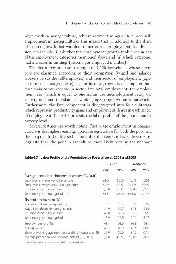
wage work in nonagriculture, self-employment in agriculture, and self-employment in nonagriculture. This means that, in addition to the shareof income growth that was due to increases in employment, the discus-sion can include (i) whether this employment growth took place in anyof the employment categories mentioned above and (ii) which categorieshad increases in earnings (income per employed member).
The decomposition uses a sample of 1,250 households whose mem-bers are classified according to their occupation (waged and salariedworkers versus the self-employed) and their sector of employment (agri-culture and nonagriculture).2 Labor income growth is decomposed intofour main terms: income in sector j to total employment, the employ-ment rate (which is equal to one minus the unemployment rate), theactivity rate, and the share of working-age people within a household.Furthermore, the first component is disaggregated into four subterms,which represent productivity gains and employment shares in each sectorof employment. Table 4.7 presents the labor profile of the population bypoverty level.
Several features are worth noting. First, wage employment in nonagri-culture is the highest earnings option in agriculture for both the poor andthe nonpoor. It should also be noted that the nonpoor have a lower earn-ings rate than the poor in agriculture, most likely because the nonpoor
Table 4.7 Labor Profile of the Population by Poverty Level, 2001 and 2005
Poor Nonpoor
2001 2005 2001 2005
Average annual labor income per worker (C$, 2001)Employed in wage work, agriculture 2,104 2,220 1,079 1,264Employed in wage work, nonagriculture 6,235 6,227 21,476 18,219Self-employed in agriculture 5,898 6,032 2,942 3,279Self-employed in nonagriculture 3,133 3,840 12,552 12,152
Share of employment (%)Waged employed in agriculture 11.2 12.4 2.5 2.9Waged employed in nonagriculture 31.9 31.7 57.8 54.8Self-employed in agriculture 41.0 39.8 9.2 9.9Self-employed in nonagriculture 15.9 16.0 30.1 31.7
Employment rate (%) 98.4 98.0 96.5 96.1Activity rate (%) 63.1 65.0 66.5 68.9Share of working-age members within a household (%) 52.9 59.0 64.2 67.1Average per capita labor income, annual (C$, 2001) 3,588 4,522 9,989 10,085
Source: Authors’calculations based on data from EMNV.
Employment and Labor Income Profile of the Population 65
work fewer hours in agricultural activities, not because they earn less perhour. Employment rates are very high among both the poor and the non-poor, but they are slightly higher for the poor, which merely reflects thefact that they cannot afford to be unemployed. Conversely, participationrates are slightly higher for the nonpoor, and dependency rates are substan-tially higher for the poor: for 2005 the poor showed 59 percent of theirmembers of working age; among the nonpoor this ratio was 67 percent.
There have been some important changes in the labor profile for theyears analyzed. First, dependency rates among the poor decreased sub-stantially, even more than for the nonpoor. Second, there was an impor-tant increase in income per worker in self-employment for both agricul-ture and nonagriculture. On the other hand, the share of the employed ineach employment category remained almost constant, with a slightincrease in waged agricultural employment.
Table 4.8 shows by quintile the same labor profile as in table 4.7,which permits a clearer understanding of labor profiles and their changesamong the poor and nonpoor households. Two important phenomenastand out. First, for the poorest 20 percent, income from nonagricultur-al wage employment is not the highest earnings option, whereas for allother quintiles it is. For the poorest 20 percent, income from self-employment is the best earnings option. Two different effects might beresponsible for this: the poor might work fewer hours as wage employ-ees in nonagriculture, and the poor might earn less per hour worked. Forthe poorest 20 percent, the highest earnings option is self-employmentin agriculture. The second phenomenon is the increase in income for thevery poor households.
Table 4.9 shows the average change in per capita household income byquintile. Between 2001 and 2005 the poor benefited more from econom-ic growth because their labor income grew substantially more than laborincome for the other groups. For the poorest quintile the annual per capi-ta labor income growth rate was 14 percent. It was about 5 percent in thesecond quintile, and it became negative in the last quintile (–1 percent).It is interesting to note that agriculture was the sector in which the poor,both the waged and salaried workers and the self-employed, saw theirincome decreasing, while the income of the poor working in other sectorsshowed a substantial increase. Despite the important growth in the percapita income of the lowest quintile, it was not sufficient to bring themabove the poverty line. In 2001 the poorest 20 percent had an average percapita income of C$2,609; the 14 percent increase still left it well belowthe C$5,241 of the poverty line. Figure 4.1 illustrates this growth.
66 Making Work Pay in Nicaragua: Employment, Growth, and Poverty Reduction
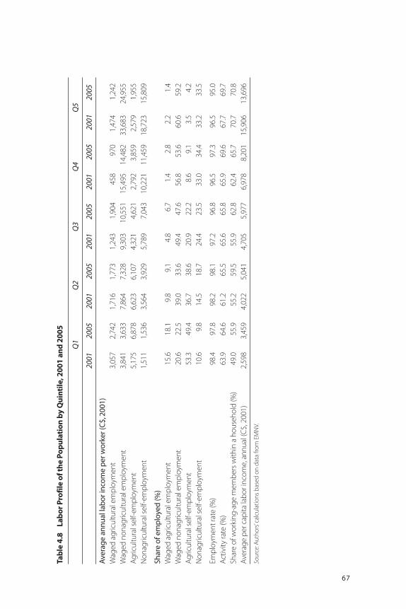
67
Tabl
e 4.
8La
bor P
rofil
e of
the
Popu
latio
n by
Qui
ntile
, 200
1 an
d 20
05
Q1
Q2
Q3
Q4
Q5
2001
2005
2001
2005
2001
2005
2001
2005
2001
2005
Ave
rag
e an
nu
al la
bor
inco
me
per
wor
ker (
C$,
2001
)W
aged
agr
icul
tura
l em
ploy
men
t3,
057
2,74
21,
716
1,77
31,
243
1,90
445
897
01,
474
1,24
2W
aged
non
agric
ultu
ral e
mpl
oym
ent
3,84
13,
633
7,86
47,
328
9,30
310
,551
15,4
9514
,482
33,6
8324
,955
Agric
ultu
ral s
elf-e
mpl
oym
ent
5,17
56,
878
6,62
36,
107
4,32
14,
621
2,79
23,
859
2,57
91,
955
Non
agric
ultu
ral s
elf-e
mpl
oym
ent
1,51
11,
536
3,56
43,
929
5,78
97,
043
10,2
2111
,459
18,7
2315
,809
Shar
e of
em
plo
yed
(%)
Wag
ed a
gric
ultu
ral e
mpl
oym
ent
15.6
18.1
9.8
9.1
4.8
6.7
1.4
2.8
2.2
1.4
Wag
ed n
onag
ricul
tura
l em
ploy
men
t20
.622
.539
.033
.649
.447
.656
.853
.660
.659
.2Ag
ricul
tura
l sel
f-em
ploy
men
t53
.349
.436
.738
.620
.922
.28.
69.
13.
54.
2N
onag
ricul
tura
l sel
f-em
ploy
men
t10
.69.
814
.518
.724
.423
.533
.034
.433
.233
.5
Empl
oym
ent r
ate
(%)
98.4
97.8
98.2
98.1
97.2
96.8
96.5
97.3
96.5
95.0
Activ
ity ra
te (%
)63
.964
.661
.265
.565
.665
.865
.969
.667
.769
.7Sh
are
of w
orki
ng-a
ge m
embe
rs w
ithin
a h
ouse
hold
(%)
49.0
55.9
55.2
59.5
55.9
62.8
62.4
65.7
70.7
70.8
Aver
age
per c
apita
labo
r inc
ome,
ann
ual (
C$, 2
001)
2,59
83,
459
4,02
25,
041
4,70
55,
977
6,97
88,
201
15,9
0613
,696
Sour
ce: A
utho
rs’c
alcu
latio
ns b
ased
on
data
from
EM
NV.
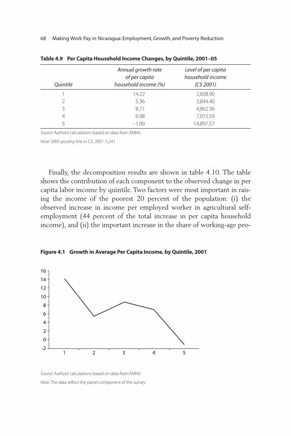
Finally, the decomposition results are shown in table 4.10. The tableshows the contribution of each component to the observed change in percapita labor income by quintile. Two factors were most important in rais-ing the income of the poorest 20 percent of the population: (i) theobserved increase in income per employed worker in agricultural self-employment (44 percent of the total increase in per capita householdincome), and (ii) the important increase in the share of working-age peo-
68 Making Work Pay in Nicaragua: Employment, Growth, and Poverty Reduction
Table 4.9 Per Capita Household Income Changes, by Quintile, 2001–05
Annual growth rate Level of per capita of per capita household income
Quintile household income (%) (C$ 2001)
1 14.22 2,608.902 5.36 3,844.403 8.71 4,862.364 6.98 7,015.595 –1.00 14,897.57
Source: Authors’calculations based on data from EMNV.
Note: 2005 poverty line in C$, 2001: 5,241
16
14
12
10
8
6
4
2
0
-21 2 3 4 5
Figure 4.1 Growth in Average Per Capita Income, by Quintile, 2001
Source: Authors’calculations based on data from EMNV.
Note: The data reflect the panel component of the survey.
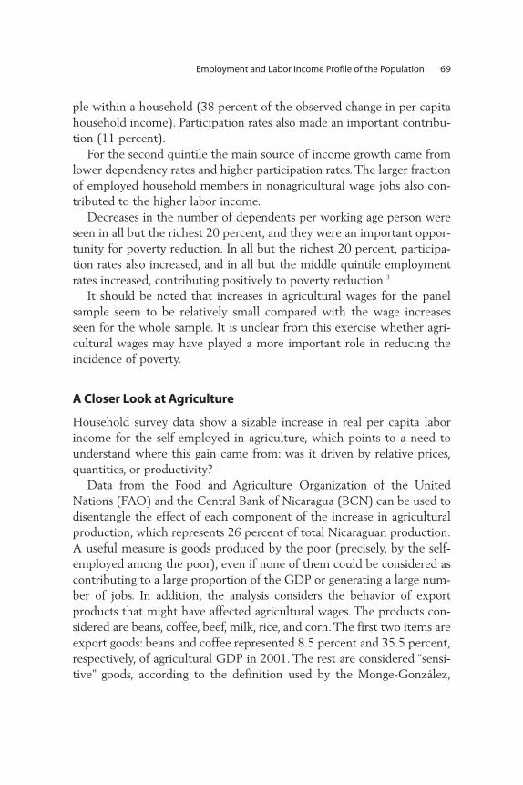
ple within a household (38 percent of the observed change in per capitahousehold income). Participation rates also made an important contribu-tion (11 percent).
For the second quintile the main source of income growth came fromlower dependency rates and higher participation rates. The larger fractionof employed household members in nonagricultural wage jobs also con-tributed to the higher labor income.
Decreases in the number of dependents per working age person wereseen in all but the richest 20 percent, and they were an important oppor-tunity for poverty reduction. In all but the richest 20 percent, participa-tion rates also increased, and in all but the middle quintile employmentrates increased, contributing positively to poverty reduction.3
It should be noted that increases in agricultural wages for the panelsample seem to be relatively small compared with the wage increasesseen for the whole sample. It is unclear from this exercise whether agri-cultural wages may have played a more important role in reducing theincidence of poverty.
A Closer Look at Agriculture
Household survey data show a sizable increase in real per capita laborincome for the self-employed in agriculture, which points to a need tounderstand where this gain came from: was it driven by relative prices,quantities, or productivity?
Data from the Food and Agriculture Organization of the UnitedNations (FAO) and the Central Bank of Nicaragua (BCN) can be used todisentangle the effect of each component of the increase in agriculturalproduction, which represents 26 percent of total Nicaraguan production.A useful measure is goods produced by the poor (precisely, by the self-employed among the poor), even if none of them could be considered ascontributing to a large proportion of the GDP or generating a large num-ber of jobs. In addition, the analysis considers the behavior of exportproducts that might have affected agricultural wages. The products con-sidered are beans, coffee, beef, milk, rice, and corn. The first two items areexport goods: beans and coffee represented 8.5 percent and 35.5 percent,respectively, of agricultural GDP in 2001. The rest are considered “sensi-tive” goods, according to the definition used by the Monge-González,
Employment and Labor Income Profile of the Population 69

Castro-Leal, Saavedra Gutiérrez (2004). The report states that sensitivegoods “are those with high tariff protection, are economically vulnerableand possess significant socio-economic importance.” This means that theyare produced by small and medium-scale farmers (see table 4.11). Beefproduction represents the largest share of GDP (4 percent in 2001), andthe production of white corn generates the largest number of jobs(175,000), or 9 percent of total employment. Figure 4.2 to figure 4.5 lookat productivity (yields), area harvested, and relative producer prices.
As for productivity changes, figure 4.2 shows the evolution of absoluteproductivity measured as yield per hectare. Productivity remained con-stant for the period under analysis for beans, coffee, and milk, while riceand maize saw increases in productivity of about 13 percent.
The United States and some Central American countries (Costa Rica,El Salvador, and Honduras) are the main trade partners of Nicaragua, sothis analysis compares relative productivity (in relation to U.S. productiv-ity) across these countries. For all products analyzed (except for drybeans), Nicaragua seems to be the least efficient country among the fourcountries in figure 4.3. In some cases, relative productivity, measured asyield per hectare of cultivated land with respect to U.S. productivity,decreased over the 15-year period analyzed, as well as over the years of
70 Making Work Pay in Nicaragua: Employment, Growth, and Poverty Reduction
Table 4.10 Shapley Decomposition of Per Capita Labor Income, by Quintile
Q1 Q2 Q3 Q4 Q1
Income per waged worker in agriculture –0.90 –17.10 –1.55 1.29 –3.30Share of employed in waged agriculture 5.15 –2.44 –1.17 2.76 –9.80Income per waged worker in nonagriculture 3.45 19.13 33.21 –3.69 289.27Share employed in waged nonagriculture 2.70 –32.69 3.02 –8.71 77.70Income per self-employed worker in 44.64 –5.14 –14.72 –3.39 55.61
agricultureShare of self-employed agriculture –14.00 3.38 –7.47 –4.90 –20.84Income per worker self-employed in 10.29 –20.86 3.28 30.82 136.31
nonagricultureShare of self-employed in nonagriculture –0.96 14.07 6.76 1.05 –31.38Employment rate 0.53 4.50 –3.74 5.46 4.00Participation rate 11.14 63.99 16.40 42.49 –342.18Inverse of dependency 37.94 73.17 65.96 36.83 –55.39Total 100 100 100 100 100
Source: Authors’calculations based on data from EMNV.
Note: Table shows the percentage share of the contribution of each component to the observed change in percapita labor.
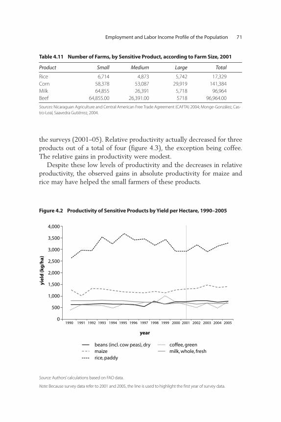
the surveys (2001–05). Relative productivity actually decreased for threeproducts out of a total of four (figure 4.3), the exception being coffee.The relative gains in productivity were modest.
Despite these low levels of productivity and the decreases in relativeproductivity, the observed gains in absolute productivity for maize andrice may have helped the small farmers of these products.
Employment and Labor Income Profile of the Population 71
Table 4.11 Number of Farms, by Sensitive Product, according to Farm Size, 2001
Product Small Medium Large Total
Rice 6,714 4,873 5,742 17,329Corn 58,378 53,087 29,919 141,384Milk 64,855 26,391 5,718 96,964Beef 64,855.00 26,391.00 5718 96,964.00
Sources: Nicaraguan Agriculture and Central American Free Trade Agreement (CAFTA) 2004; Monge-González, Cas-tro-Leal, Saavedra Gutiérrez, 2004.
1990 1991 1992 1993 1994 1995 1996 1997 1998 1999 2000 2001 2002 2003 2004 2005
year
yiel
d (k
g/h
a)
4,000
3,500
3,000
2,500
2,000
1,500
1,000
500
0
beans (incl. cow peas), dry coffee, greenmaize milk, whole, freshrice, paddy
Figure 4.2 Productivity of Sensitive Products by Yield per Hectare, 1990–2005
Source: Authors’calculations based on FAO data.
Note: Because survey data refer to 2001 and 2005, the line is used to highlight the first year of survey data.
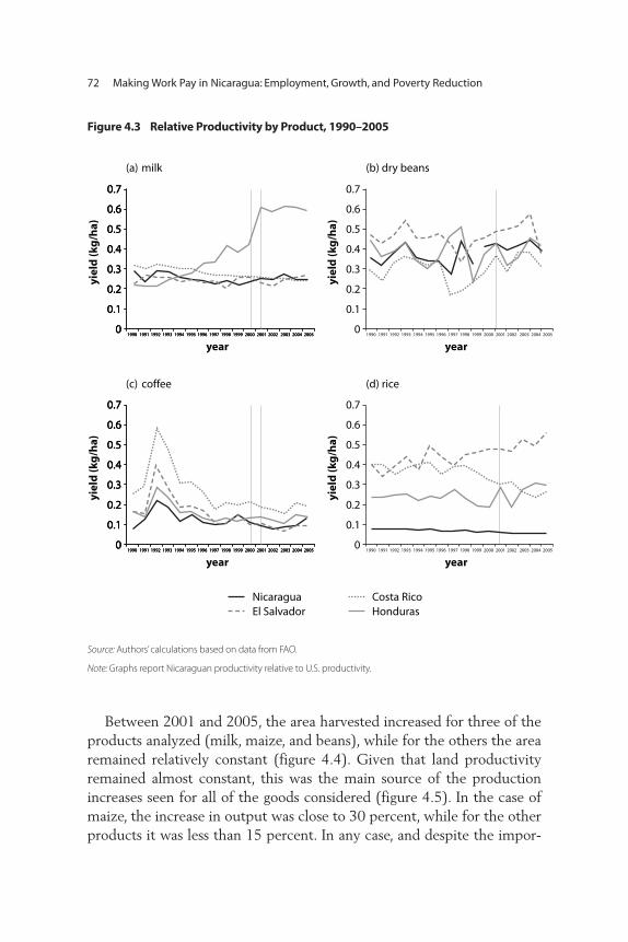
Between 2001 and 2005, the area harvested increased for three of theproducts analyzed (milk, maize, and beans), while for the others the arearemained relatively constant (figure 4.4). Given that land productivityremained almost constant, this was the main source of the productionincreases seen for all of the goods considered (figure 4.5). In the case ofmaize, the increase in output was close to 30 percent, while for the otherproducts it was less than 15 percent. In any case, and despite the impor-
72 Making Work Pay in Nicaragua: Employment, Growth, and Poverty Reduction
1990 1991 1992 1993 1994 1995 1996 1997 1998 1999 2000 2001 2002 2003 2004 2005
0.7
0.6
0.5
0.4
0.3
0.2
0.1
0yi
eld
(kg
/ha)
year1990 1991 1992 1993 1994 1995 1996 1997 1998 1999 2000 2001 2002 2003 2004 2005
0.7
0.6
0.5
0.4
0.3
0.2
0.1
0
yiel
d (k
g/h
a)
year1990 1991 1992 1993 1994 1995 1996 1997 1998 1999 2000 2001 2002 2003 2004 2005
0.7
0.6
0.5
0.4
0.3
0.2
0.1
01990 1991 1992 1993 1994 1995 1996 1997 1998 1999 2000 2001 2002 2003 2004 2005
0.7
0.6
0.5
0.4
0.3
0.2
0.1
0
1990 1991 1992 1993 1994 1995 1996 1997 1998 1999 2000 2001 2002 2003 2004 2005
0.7
0.6
0.5
0.4
0.3
0.2
0.1
0
yiel
d (k
g/h
a)
year1990 1991 1992 1993 1994 1995 1996 1997 1998 1999 2000 2001 2002 2003 2004 2005
0.7
0.6
0.5
0.4
0.3
0.2
0.1
0
yiel
d (k
g/h
a)
year1990 1991 1992 1993 1994 1995 1996 1997 1998 1999 2000 2001 2002 2003 2004 2005
0.7
0.6
0.5
0.4
0.3
0.2
0.1
01990 1991 1992 1993 1994 1995 1996 1997 1998 1999 2000 2001 2002 2003 2004 2005
0.7
0.6
0.5
0.4
0.3
0.2
0.1
0
Nicaragua Costa RicoEl Salvador Honduras
(a) milk
(c) coffee
(b) dry beans
(d) rice
Figure 4.3 Relative Productivity by Product, 1990–2005
Source: Authors’calculations based on data from FAO.
Note: Graphs report Nicaraguan productivity relative to U.S. productivity.
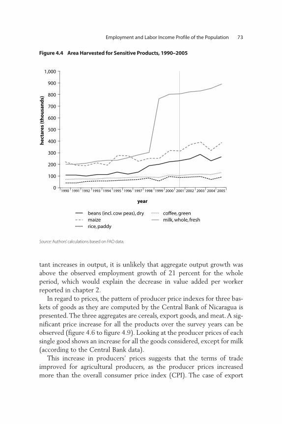
tant increases in output, it is unlikely that aggregate output growth wasabove the observed employment growth of 21 percent for the wholeperiod, which would explain the decrease in value added per workerreported in chapter 2.
In regard to prices, the pattern of producer price indexes for three bas-kets of goods as they are computed by the Central Bank of Nicaragua ispresented.The three aggregates are cereals, export goods, and meat.A sig-nificant price increase for all the products over the survey years can beobserved (figure 4.6 to figure 4.9). Looking at the producer prices of eachsingle good shows an increase for all the goods considered, except for milk(according to the Central Bank data).
This increase in producers’ prices suggests that the terms of tradeimproved for agricultural producers, as the producer prices increasedmore than the overall consumer price index (CPI). The case of export
Employment and Labor Income Profile of the Population 73
1,000
900
800
700
600
500
400
300
200
100
0 1990 1991 1992 1993 1994 1995 1996 1997 1998 1999 2000 2001 2002 2003 2004 2005
year
hec
tare
s (t
ho
usa
nd
s)
beans (incl. cow peas), dry coffee, greenmaize milk, whole, freshrice, paddy
Figure 4.4 Area Harvested for Sensitive Products, 1990–2005
Source: Authors’calculations based on FAO data.
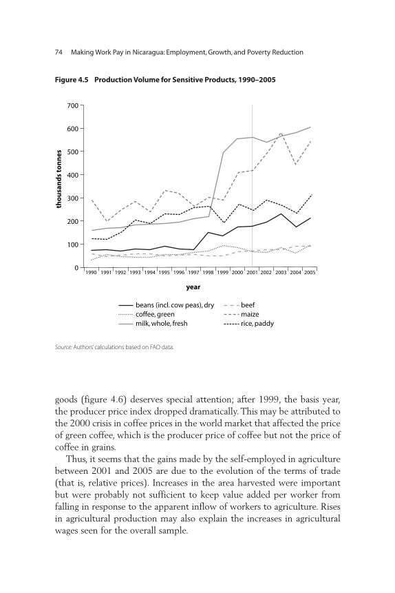
goods (figure 4.6) deserves special attention; after 1999, the basis year,the producer price index dropped dramatically. This may be attributed tothe 2000 crisis in coffee prices in the world market that affected the priceof green coffee, which is the producer price of coffee but not the price ofcoffee in grains.
Thus, it seems that the gains made by the self-employed in agriculturebetween 2001 and 2005 are due to the evolution of the terms of trade(that is, relative prices). Increases in the area harvested were importantbut were probably not sufficient to keep value added per worker fromfalling in response to the apparent inflow of workers to agriculture. Risesin agricultural production may also explain the increases in agriculturalwages seen for the overall sample.
74 Making Work Pay in Nicaragua: Employment, Growth, and Poverty Reduction
700
600
500
400
300
200
100
0 1990 1991 1992 1993 1994 1995 1996 1997 1998 1999 2000 2001 2002 2003 2004 2005
year
tho
usa
nd
s to
nn
es
beans (incl. cow peas), dry beefcoffee, green maizemilk, whole, fresh rice, paddy
Figure 4.5 Production Volume for Sensitive Products, 1990–2005
Source: Authors’calculations based on FAO data.
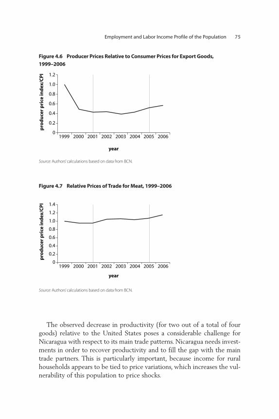
The observed decrease in productivity (for two out of a total of fourgoods) relative to the United States poses a considerable challenge forNicaragua with respect to its main trade patterns. Nicaragua needs invest-ments in order to recover productivity and to fill the gap with the maintrade partners. This is particularly important, because income for ruralhouseholds appears to be tied to price variations, which increases the vul-nerability of this population to price shocks.
Employment and Labor Income Profile of the Population 75
1.2
1.0
0.8
0.6
0.4
0.2
01999 2000 2001 2002 2003 2004 2005 2006
year
pro
du
cer
pri
ce in
dex
/CP
I
Figure 4.6 Producer Prices Relative to Consumer Prices for Export Goods,1999–2006
Source: Authors’calculations based on data from BCN.
1.4
1.2
1.0
0.8
0.6
0.4
0.2
01999 2000 2001 2002 2003 2004 2005 2006
year
pro
du
cer
pri
ce in
dex
/CP
I
Figure 4.7 Relative Prices of Trade for Meat, 1999–2006
Source: Authors’calculations based on data from BCN.

76 Making Work Pay in Nicaragua: Employment, Growth, and Poverty Reduction
1.4
1.2
1.0
0.8
0.6
0.4
01999 2000 2001 2002 2003 2004 2005 2006
year
pro
du
cer
pri
ce in
dex
/CP
I
Figure 4.8 Relative Prices for Cereals, 1999–2006
Source: Authors’calculations based on data from BCN.
250
200
150
100
50
01999 2000 2001 2002 2003 2004 2005 2006
year
pro
du
cer
pri
ce in
dex
/CP
I
coffee, green rice, paddybeans, dry meatmilk, whole, fresh maize
Figure 4.9 Relative Prices for Sensitive Products, 2001–06
Source: Authors’calculations based on data from BCN.

Notes
1. See Kakwani, Neri, and Son (2006) for an application of this decomposition tothe analysis of pro-poor rates of growth.
2. Some methodological clarifications are important. First, people of working ageare selected by dropping child laborers and the working elderly. This mightimply overestimating productivity and underestimating employment sharesand thus their contribution to total labor income growth. This is not a seriousissue as they represent less than 2 percent and 7 percent, respectively, of thetotal working population (average over the two years of the survey). Second,a little over one-third of the sample is dropped in both 2001 and 2005 becausethere is no correspondence between workers and reported income withinhouseholds. Some households report income in a sector where no one isemployed and vice versa. It might be an issue of misreported income for someof the households. Additionally, in many cases it seems that many peoplereporting earnings from agricultural self-employment are actually receivingrents from farms and are not directly employed in agriculture. Because this isnot labor income but rents, these households are dropped from the sample.Finally, the analysis drops a small number of households that report a jump inthe employment rate from 0 to 1, as they have an analogous increase in incomeand therefore a growth rate of income that goes to infinity. The selection iscompletely neutral across quintiles because it drops proportionally more poorthan rich households as they are more likely to suffer from misreportedincome in agricultural business.
3. An interpretation is risky given the small number of households in each quin-tile. For these estimations the analysis excluded the 2.5 percent in the tails ofchanges in total labor income, and results change when these outliers areincluded. Additionally, the sample selected shows no increase in wages exceptfor the third and fourth quintiles, and agricultural wage increases are lowerthan for the whole sample.
Employment and Labor Income Profile of the Population 77
Annex 4ADecomposition of Labor Income Growth
The labor income profile is best described at the household level. A sim-ple and useful characterization of households in terms of labor indicatorscan be obtained by noting that the average labor income of household jcan be written as (borrowing from Kakwani, Neri, and Son 2006):
(A–1)
where is the total labor income of household j; Hj is the total hoursworked by working-age members of household, j; Ej is the total numberof employed in the household; Lj is the number of participants in thelabor market; and Aj is the number of working-age members. In this way
=IL/H corresponds to average earnings per hour worked, h = H/E cor-responds to average hours worked, E/L is the employment rate, l = L/A isthe participation rate, and a = A/N is the ratio of working-age membersto total household members, or the dependency rate. For simplicity, letthe above equation be rewritten as:
(A–2)
where (1 – uj) corresponds to the employment rate of household j, whichcan be rewritten as 1 minus the household’s unemployment rate uj. Notethat (omega bar) is different from (simple omega) which refers tooutput per worker in the decomposition of GDP per capita.
In many contexts there is an important fraction of child laborers andelderly workers, and calculating earnings per hour worked by theemployed of working age is overestimating real household productivity.In these cases, it might be better to abstract from the structure of thehousehold according to working age (Aj in equation A1) and calculatedependency rates as the number of participating individuals over the totalof working household members (Aj/Lj). Define Ej as the number of work-ing individuals irrespective of whether they are of working age or not anddefine hours worked, Hj, as total hours worked for all employed individ-uals irrespective of age.
78 Making Work Pay in Nicaragua: Employment, Growth, and Poverty Reduction
I
N
I
H
H
E
E
L
L
A
A
NjL
j
jL
j
j
j
j
j
j
j
j
j
=
ι ϖjL
j j j j jh u l a= −( )1
I jL
ϖ
ϖ
By averaging each of the components of the household’s per capitalabor income over subgroups of population, we can obtain a full profileof labor market characteristics. For example, if we divide households byquintile of income, it will describe the average labor market characteris-tics of each quintile. Let denote the subset of households belonging toa particular quintile. It is possible to compare deciles by average depend-ency rates,
,
average participation rates,
,
average hours worked,
,
incidence of unemployment,
,
and earnings per hour worked
.
A traditional way to understand how labor markets have affected wel-fare is to disentangle the sources of labor income growth that are respon-sible for observed changes in total labor income.1
From equation A2, the average per capita labor income of the subset of households (whether poor or nonpoor households, or householdsfalling within an income range or with particular demographic character-istics) will then be:
(A–3)
Employment and Labor Income Profile of the Population 79
1N
ajjΩ Ω∈∑
1N
ljjΩ Ω∈∑
1N
hjjΩ Ω∈∑
1N
ujjΩ Ω∈∑
1N j
jΩ Ω
ϖ∈∑
1 11
N N
h u
jL
j
j jj
jjj
Ω Ω Ω
Ω Ωln
ln ln ln( )
ιϖ
∈
∈ ∈∑∑ ∑
=+ + −
∈∈
∈ ∈
∑∑ ∑+ +
⎛
⎝
⎜⎜⎜
⎞
⎠
Ω
Ω Ω
ln lnl ajj
jj
⎟⎟⎟⎟
It is thus possible to decompose the change in the average per capitahousehold labor income of group into changes in its different compo-nents: changes in average log earnings per hour worked, changes in aver-age of log hours worked, changes in average log unemployment rates, andso forth. In particular:
(A–4)
In this way we can easily see whether growth in the average laborincome of the poor (or any group ) was due to changes in employmentrates, participation rates, hours of work, or earnings per hour worked.
We can go a step further and decompose average earnings per hourinto earnings per hour from self-employment (j) and earnings per hourfrom wage employment (wj):
,
with corresponding to the share of wage employment in total hoursworked and corresponding to the share of self-employment. In thiscase, however, log-linearization of equation A2 is no longer possible, andwe would have to perform Shapley decompositions to analyze incomechanges.
Comparing changes in average incomes of the poor, and their compo-nents, with changes in average incomes of the nonpoor can shed some lighton what the channels are through which a growth process is affecting theincome of the poor. In many cases, however, there might be considerableheterogeneity among employment sectors. In these cases it is useful to per-form these decompositions by disaggregating households according toother characteristics: for example, dividing households depending on theirmain occupation (e.g., differentiating between rural farmers, rural nonfarmworkers, sector of occupation of household head, and so forth).
Note
1. See Kakwani, Neri, and Son (2006) for an application of this decomposition tothe analysis if pro-poor rates of growth.
80 Making Work Pay in Nicaragua: Employment, Growth, and Poverty Reduction
∆ ∆ ∆Ω Ω Ω Ω ΩΩ
1 1 1N N N
hjL
jj j
jj
ln ln lnι ϖ∈ ∈∈∑ ∑∑= +
ln( )+ − +∈∑∆ ∆
Ω Ω Ω
11
1N
uNj
j
lln lnlN
ajj
jj∈ ∈
∑ ∑+Ω Ω Ω
∆ 1
ϖ ππjL
jw
j j jh w h= +
hjw
hjπ
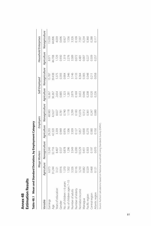
81
Ann
ex 4
BEs
timat
ion
Resu
lts
Tabl
e 4B
.1M
ean
and
Stan
dard
Dev
iatio
n, b
y Em
ploy
men
t Cat
egor
y
Wag
e W
orke
rsEm
ploy
ers
Self-
Empl
oyed
Hou
seho
ld E
nter
prise
s
Varia
ble
Agric
ultu
reN
onag
ricul
ture
Agric
ultu
reN
onag
ricul
ture
Agric
ultu
reN
onag
ricul
ture
Agric
ultu
reN
onag
ricul
ture
Earn
ings
6.07
313
.240
29.2
9348
.983
16.3
6715
.787
8.07
115
.039
Age
31.2
4432
.716
42.3
2042
.627
36.3
6739
.438
44.7
0844
.896
Year
s of
edu
catio
n3.
121
8.40
73.
339
8.02
72.
654
5.37
51.
729
4.03
9G
ende
r0.
916
0.53
70.
949
0.78
10.
885
0.39
30.
930
0.69
6N
o. o
f chi
ldre
n <
6 y
ears
1.37
00.
878
0.97
60.
740
1.32
30.
904
1.31
90.
927
No.
of c
hild
ren
ages
7–1
51.
502
1.29
61.
506
1.11
81.
281
1.34
62.
276
1.55
6N
umbe
r of a
dults
3.32
63.
549
3.50
93.
299
2.87
93.
146
3.58
93.
326
Num
ber o
f eld
erly
0.11
60.
200
0.12
70.
183
0.16
90.
133
0.07
20.
109
Non
labo
r inc
ome
3.21
010
.529
5.85
715
.076
3.65
38.
364
4.48
17.
597
Man
agua
0.08
20.
431
0.00
00.
312
0.04
60.
383
0.00
70.
234
Paci
fic re
gion
0.32
90.
303
0.27
00.
361
0.20
80.
348
0.22
70.
360
Cent
ral r
egio
n0.
468
0.19
70.
580
0.24
70.
520
0.21
10.
509
0.28
8A
tlant
ic re
gion
0.12
10.
070
0.15
00.
080
0.22
60.
058
0.25
70.
117
Sour
ce: A
utho
rs’c
alcu
latio
ns b
ased
on
Nat
iona
l Hou
seho
ld L
ivin
g St
anda
rds
Surv
ey (E
MN
V).
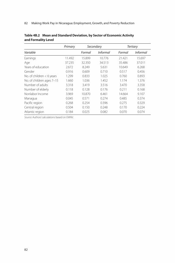
82
Table 4B.2 Mean and Standard Deviation, by Sector of Economic Activity and Formality Level
Primary Secondary Tertiary
Variable Formal Informal Formal Informal
Earnings 11.492 15.899 10.776 21.421 15.697Age 37.235 32.350 34.513 35.486 37.011Years of education 2.672 8.249 5.631 10.649 6.268Gender 0.916 0.609 0.710 0.517 0.456No. of children < 6 years 1.299 0.833 1.025 0.760 0.893No. of children ages 7–15 1.660 1.036 1.452 1.174 1.376Number of adults 3.318 3.419 3.516 3.470 3.358Number of elderly 0.118 0.128 0.176 0.211 0.168Nonlabor Income 3.969 10.870 6.461 14.664 9.107Managua 0.045 0.571 0.274 0.485 0.374Pacific region 0.268 0.254 0.396 0.275 0.329Central region 0.504 0.150 0.248 0.170 0.224Atlantic region 0.184 0.025 0.082 0.070 0.074
Source: Authors’calculations based on EMNV.
82 Making Work Pay in Nicaragua: Employment, Growth, and Poverty Reduction
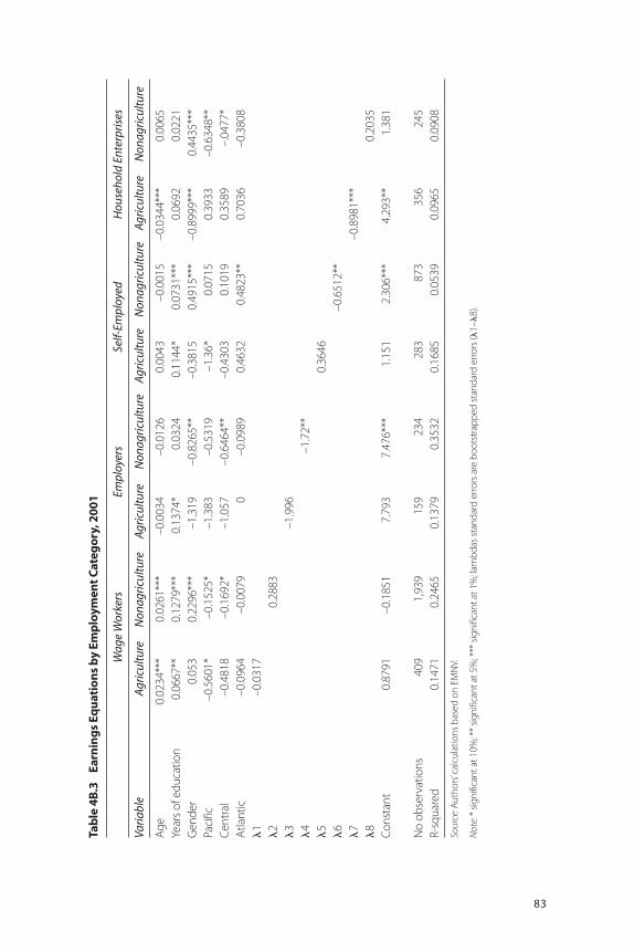
83
Tabl
e 4B
.3Ea
rnin
gs E
quat
ions
by
Empl
oym
ent C
ateg
ory,
200
1
Wag
e W
orke
rsEm
ploy
ers
Self-
Empl
oyed
Hou
seho
ld E
nter
prise
s
Varia
ble
Agric
ultu
reN
onag
ricul
ture
Agric
ultu
reN
onag
ricul
ture
Agric
ultu
reN
onag
ricul
ture
Agric
ultu
reN
onag
ricul
ture
Age
0.02
34**
*0.
0261
***
–0.0
034
–0.0
126
0.00
43–0
.001
5–0
.034
4***
0.00
65Ye
ars
of e
duca
tion
0.06
67**
0.12
79**
*0.
1374
*0.
0324
0.11
44*
0.07
31**
*0.
0692
0.02
21G
ende
r0.
053
0.22
96**
*–1
.319
–0.8
265*
*–0
.381
50.
4915
***
–0.8
999*
**0.
4435
***
Paci
fic–0
.560
1*–0
.152
5*–1
.383
–0.5
319
–1.3
6*0.
0715
0.39
33–0
.634
8**
Cent
ral
–0.4
818
–0.1
692*
–1.0
57–0
.646
4**
–0.4
303
0.10
190.
3589
–.04
77*
Atla
ntic
–0.0
964
–0.0
079
0–0
.098
90.
4632
0.48
23**
0.70
36–0
.380
8
1–0
.031
7
20.
2883
3
–1.9
96
4–1
.72*
*
50.
3646
6
–0.6
512*
*
7–0
.898
1***
8
0.20
35Co
nsta
nt0.
8791
–0.1
851
7.79
37.
476*
**1.
151
2.30
6***
4.29
3**
1.38
1
No
obse
rvat
ions
409
1,93
915
923
428
387
335
624
5R-
squa
red
0.14
710.
2465
0.13
790.
3532
0.16
850.
0539
0.09
650.
0908
Sour
ce: A
utho
rs’c
alcu
latio
ns b
ased
on
EMN
V.
Not
e: *
signi
fican
t at 1
0%; *
* sig
nific
ant a
t 5%
; ***
sig
nific
ant a
t 1%
; lam
bdas
sta
ndar
d er
rors
are
boo
tstr
appe
d st
anda
rd e
rrors
(1–
8)
.

Table 4B.4 Earnings Equations by Sector of Employment, 2001
Primary Secondary Tertiary
Variable Formal Informal Formal Informal
Age 0.0045 0.014 0.0354*** 0.027*** 0.0253***Years of education –0.0356 0.1181*** 0.0649*** 0.177*** 0.0715***Gender 0.8978* 0.2768 0.1972 0.2212** 0.1668Pacific region 0.0546 –0.3224* –0.3854*** –0.2501** –0.0094Central region 0.8212 –0.1309 –0.405*** –0.3088* –0.063Atlantic region 1.399** –0.5493 –0.1137 –0.0783 0.2034Ï1 1.109*Ï2 1.066*Ï3 –0.0587Ï4 0.7258Ï5 0.1745Constant –1.017 –1.189 0.4249 –1.142 0.3396
No observations 1,210 219 569 693 1,812R-squared 0.0814 0.2304 0.159 0.2732 0.1097
Source: Authors’calculations based on EMNV.
Note: * significant at 10%; ** significant at 5%; *** significant at 1%; lambdas standard errors are bootstrapped standard errors.
84 Making Work Pay in Nicaragua: Employment, Growth, and Poverty Reduction

85
Tabl
e 4B
.5O
axac
a-Bl
inde
r Dec
ompo
sitio
n: D
etai
led
Out
com
es fo
r Sec
tor a
nd In
form
ality
Seco
ndar
y In
form
al v
s. Te
rtia
ry In
form
al v
s. Se
cond
ary
Form
al v
s. Te
rtia
ry F
orm
al v
s. Se
cond
ary
Prim
ary
Tert
iary
Prim
ary
Seco
ndar
y In
form
alTe
rtia
ry In
form
al
Coef
ficie
nts
P-va
lue
Coef
ficie
nts
P-va
lue
Coef
ficie
nts
P-va
lue
Coef
ficie
nts
P-va
lue
Net
diff
eren
ce1.
326
0.08
31.
234
0.01
81.
598
0.17
10.
110
0.85
6
End
owm
ents
Age
–0.0
120.
245
–0.0
010.
257
0.03
00.
158
0.04
10.
000
Year
s of
edu
catio
n–0
.105
0.54
9–0
.128
0.54
9–0
.309
0.00
0–0
.775
0.00
1G
ende
r–0
.184
0.09
7–0
.413
0.09
70.
028
0.09
8–0
.013
0.01
0Pa
cific
regi
on0.
007
0.90
20.
003
0.90
2–0
.046
0.07
4–0
.014
0.04
5Ce
ntra
l reg
ion
–0.2
100.
212
–0.2
300.
212
–0.0
130.
660
–0.0
160.
050
Atla
ntic
regi
on–0
.143
0.03
8–0
.154
0.03
8–0
.031
0.16
40.
000
0.54
5To
tal
–0.6
480.
150
–0.9
220.
170
–0.3
410.
002
–0.7
780.
002
Coe
ffic
ien
tsAg
e1.
150
0.00
00.
774
0.00
00.
692
0.06
0–0
.060
0.80
2Ye
ars
of e
duca
tion
0.26
80.
102
0.28
60.
075
–0.4
390.
064
–1.1
230.
060
Gen
der
–0.6
420.
210
–0.6
700.
190
–0.0
480.
716
–0.0
280.
731
Paci
fic re
gion
–0.1
180.
343
–0.0
170.
888
–0.0
160.
783
0.06
60.
131
Cent
ral r
egio
n–0
.618
0.06
9–0
.446
0.18
5–0
.041
0.40
70.
042
0.20
7A
tlant
ic re
gion
–0.2
780.
031
–0.2
200.
081
0.01
10.
326
0.02
00.
122
Cons
tant
1.44
20.
302
1.35
60.
301
1.61
40.
116
1.48
10.
240
Tota
l1.
205
0.11
01.
065
0.05
81.
773
0.13
50.
398
0.51
2
Inte
ract
ion
Age
–0.0
840.
000
–0.0
050.
001
0.04
60.
061
–0.0
030.
802
Year
s of
edu
catio
n0.
297
0.10
20.
385
0.07
50.
139
0.06
40.
462
0.06
0G
ende
r0.
144
0.21
00.
336
0.19
0–0
.008
0.71
60.
003
0.73
1Pa
cific
regi
on–0
.057
0.34
3–0
.004
0.88
8–0
.009
0.78
30.
013
0.13
1Ce
ntra
l reg
ion
0.31
40.
069
0.24
80.
185
–0.0
270.
408
0.01
30.
208
Atla
ntic
regi
on0.
154
0.03
20.
132
0.08
10.
025
0.32
60.
001
0.14
3To
tal
0.76
90.
090
1.09
20.
108
0.16
70.
174
0.49
00.
049
Sour
ce: A
utho
rs’c
alcu
latio
ns b
ased
on
EMN
V.
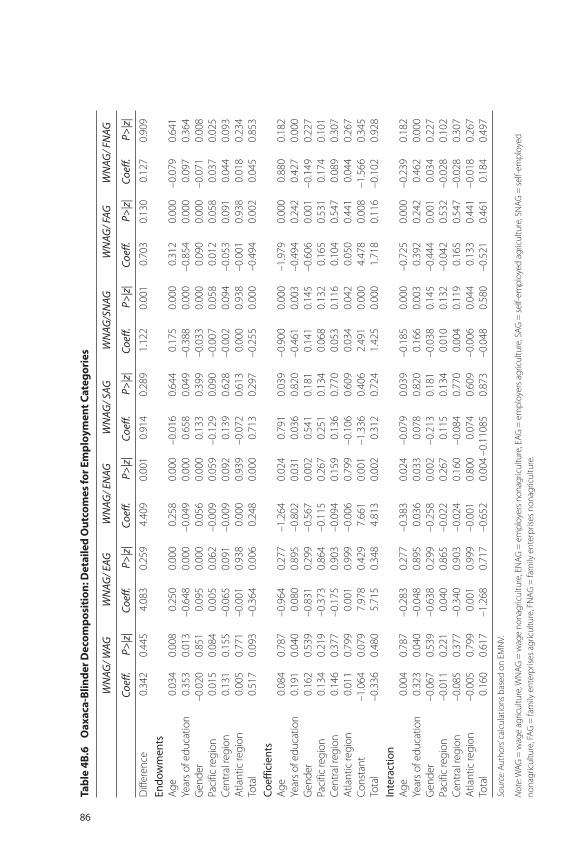
86
Tabl
e 4B
.6O
axac
a-Bl
inde
r Dec
ompo
sitio
n: D
etai
led
Out
com
es fo
r Em
ploy
men
t Cat
egor
ies
WN
AG/ W
AGW
NAG
/ EAG
WN
AG/ E
NAG
WN
AG/ S
AGW
NAG
/SN
AGW
NAG
/ FAG
WN
AG/ F
NAG
Coef
f.P>
|z|
Coef
f.P>
|z|
Coef
f.P>
|z|
Coef
f.P>
|z|
Coef
f.P>
|z|
Coef
f.P>
|z|
Coef
f.P>
|z|
Diff
eren
ce0.
342
0.44
54.
083
0.25
94.
409
0.00
10.
914
0.28
91.
122
0.00
10.
703
0.13
00.
127
0.90
9En
dow
men
tsAg
e0.
034
0.00
80.
250
0.00
00.
258
0.00
0–0
.016
0.64
40.
175
0.00
00.
312
0.00
0–0
.079
0.64
1Ye
ars
of e
duca
tion
0.35
30.
013
–0.6
480.
000
–0.0
490.
000
0.65
80.
049
–0.3
880.
000
–0.8
540.
000
0.09
70.
364
Gen
der
–0.0
200.
851
0.09
50.
000
0.05
60.
000
0.13
30.
399
–0.0
330.
000
0.09
00.
000
–0.0
710.
008
Paci
fic re
gion
0.01
50.
084
0.00
50.
062
–0.0
090.
059
–0.1
290.
090
–0.0
070.
058
0.01
20.
058
0.03
70.
025
Cent
ral r
egio
n0.
131
0.15
5–0
.065
0.09
1–0
.009
0.09
20.
139
0.62
8–0
.002
0.09
4–0
.053
0.09
10.
044
0.09
3A
tlant
ic re
gion
0.00
50.
771
–0.0
010.
938
0.00
00.
939
–0.0
720.
613
0.00
00.
938
–0.0
010.
938
0.01
80.
234
Tota
l0.
517
0.09
3–0
.364
0.00
60.
248
0.00
00.
713
0.29
7–0
.255
0.00
0–0
.494
0.00
20.
045
0.85
3C
oeff
icie
nts
Age
0.08
40.
787
–0.9
640.
277
–1.2
640.
024
0.79
10.
039
–0.9
000.
000
–1.9
790.
000
0.88
00.
182
Year
s of
edu
catio
n0.
191
0.04
00.
080
0.89
5–0
.802
0.03
10.
036
0.82
0–0
.461
0.00
3–0
.494
0.24
20.
427
0.00
0G
ende
r0.
162
0.53
9–0
.831
0.29
9–0
.567
0.00
20.
541
0.18
10.
141
0.14
5–0
.606
0.00
1–0
.149
0.22
7Pa
cific
regi
on0.
134
0.21
9–0
.373
0.86
4–0
.115
0.26
70.
251
0.13
40.
068
0.13
20.
165
0.53
10.
174
0.10
1Ce
ntra
l reg
ion
0.14
60.
377
–0.1
750.
903
–0.0
940.
159
0.13
60.
770
0.05
30.
116
0.10
40.
547
0.08
90.
307
Atla
ntic
regi
on0.
011
0.79
90.
001
0.99
9–0
.006
0.79
9–0
.106
0.60
90.
034
0.04
20.
050
0.44
10.
044
0.26
7Co
nsta
nt–1
.064
0.07
97.
978
0.42
97.
661
0.00
1–1
.336
0.40
62.
491
0.00
04.
478
0.00
8–1
.566
0.34
5To
tal
–0.3
360.
480
5.71
50.
348
4.81
30.
002
0.31
20.
724
1.42
50.
000
1.71
80.
116
–0.1
020.
928
Inte
ract
ion
Age
0.00
40.
787
–0.2
830.
277
–0.3
830.
024
–0.0
790.
039
–0.1
850.
000
–0.7
250.
000
–0.2
390.
182
Year
s of
edu
catio
n0.
323
0.04
0–0
.048
0.89
50.
036
0.03
30.
078
0.82
00.
166
0.00
30.
392
0.24
20.
462
0.00
0G
ende
r–0
.067
0.53
9–0
.638
0.29
9–0
.258
0.00
2–0
.213
0.18
1–0
.038
0.14
5–0
.444
0.00
10.
034
0.22
7Pa
cific
regi
on–0
.011
0.22
10.
040
0.86
5–0
.022
0.26
70.
115
0.13
40.
010
0.13
2–0
.042
0.53
2–0
.028
0.10
2Ce
ntra
l reg
ion
–0.0
850.
377
–0.3
400.
903
–0.0
240.
160
–0.0
840.
770
0.00
40.
119
0.16
50.
547
–0.0
280.
307
Atla
ntic
regi
on–0
.005
0.79
90.
001
0.99
9–0
.001
0.80
00.
074
0.60
9–0
.006
0.04
40.
133
0.44
1–0
.018
0.26
7To
tal
0.16
00.
617
–1.2
680.
717
–0.6
520.
004
–0.1
1085
0.87
3–0
.048
0.58
0–0
.521
0.46
10.
184
0.49
7
Sour
ce: A
utho
rs’c
alcu
latio
ns b
ased
on
EMN
V.
Not
e: W
AG =
wag
e ag
ricul
ture
, WN
AG =
wag
e no
nagr
icul
ture
, EN
AG =
em
ploy
ers
nona
gric
ultu
re, E
AG =
em
ploy
ers
agric
ultu
re, S
AG =
sel
f-em
ploy
ed a
gric
ultu
re, S
NAG
= s
elf-e
mpl
oyed
nona
gric
ultu
re, F
AG =
fam
ily e
nter
prise
s ag
ricul
ture
, FN
AG =
fam
ily e
nter
prise
s no
nagr
icul
ture
.
The objective of this chapter is twofold. The first objective is to identifythe relevant dimensions across which the labor market is segmented (inother words, which are the good jobs sectors and which are the bad jobssectors). The second objective is to analyze the role of skills in employ-ment and earnings and to see whether skills are posing a constraint toemployment growth in the good jobs sector.
The chapter is organized as follows. The first section briefly describesbasic assumptions of a model of labor market segmentation, the secondconsiders whether there is any evidence of segmentation and, if so, acrosswhich dimensions. It also points toward the possible causes of segmen-tation. The third section discusses the barriers to mobility. The last sec-tion deals with skill mismatch and the role of skills in earnings andemployment.
Labor Market Segmentation: Basic Assumptions and Literature Review
There is a growing consensus that labor markets in developing countriesare segmented, and that this segmentation has important implications forthe extent to which the poor benefit from growth and from earnings
C H A P T E R 5
Segmentation and Skill Mismatch
87
opportunities.1 At the core of this model are the following premisesregarding the country’s markets:
• The labor market consists of various segments that offer qualitative,distinct types of employment for individuals with identical productivi-ty endowments—that is, the good jobs sector and the bad jobs sector.2
• There is limited mobility between sectors and barriers of access togood jobs, so that not all those seeking work in the good jobs sectorcan find it.
• Of good job and bad job sectors, wage and employment levels are notcompetitively determined in at least one of the sectors. There are dif-ferences in marginal productivity between those two sectors.
The bad jobs sector is a free-entry sector, that is, no skills or capital andno special connections or qualities are needed to enter. Returns to laborin this sector are low, and households that earn a living in the sector aremore likely to be poorer than other households.
However, there is no consensus as to which are the segments of thelabor market and, among them, which segments should be of concernregarding pro-poor employment and labor market policies. Is the marketsegmented across the formal-informal divide? Or is it segmented acrossthe self-employment–wage-employment divide? Are labor markets seg-mented between urban and rural areas or between agriculture and nona-griculture, or both? And which of these segments are most relevant forthe poor?
Moreover, it is not easy to prove segmentation empirically because it ishard to distinguish whether workers are in a particular sector because ofchoice or lack of other employment options. For example, Maloney(2004) finds evidence that in Argentina, Brazil, and Mexico many work-ers are in the informal sector because they value the implied flexibilityand the ability to report a higher job status. These workers place a lowvalue on social security benefits because they do not believe that the gov-ernments will reliably deliver these benefits. If the analysis controls forskills, earnings in the informal sector do not differ substantially from thosein the formal sector. This has led to the conclusion that workers opt forthe informal sector because, given their level of skills, it offers them thehighest returns.
In addition to the difficulty of identifying whether markets are seg-mented and, if so, across which dimensions, it can be difficult to disen-
88 Making Work Pay in Nicaragua: Employment, Growth, and Poverty Reduction
tangle the causes of segmentation. In many cases segmentation thatresults from noncompetitive wage-setting mechanisms may be inter-twined with extensive barriers to moving between good and bad jobs.For example, job location, skills requirements, or ethnic or gender dis-crimination may play a role.
In addition to segmentation, the size of the bad jobs sector (whether itis informal or formal) might be affected by “skill mismatch,” that is, by thefact that the available skills of the workforce do not match the skillsdemanded by the good jobs sector. For example, it has been widely notedthat technological change increases the relative demand for skills. Thisusually increases skill premiums, which may widen the income gapbetween the good jobs sector and the bad jobs sector (as has happened inother Latin American countries). In this case, the gap is not due to seg-mentation but to differences in the individual characteristics of thoseemployed in each sector, with the good jobs sector reducing its share ofunskilled workers and the redundant labor force being shed to the badjobs sector. In extreme cases, the lack of skills can become a binding con-straint to growth.
In general, the relationships between education and skills, employ-ment, and poverty under segmented labor markets are complex and arenot reduced to the role of skill mismatch. In segmented labor markets, ifjobs are rationed, it is tempting to conclude that increasing the level ofeducation of the labor force may not help those employed in the bad jobssector to get a job. Because there are no jobs, jobs are by definitionrationed. However, jobs may be rationed for the low skilled but not forthe skilled. For example, non-market-clearing wages like minimum wagesmay affect the unskilled but not the skilled labor force; and barriers tomobility due to lack of information may be stronger for the unskilled. Ifthis is the case, increasing the level of education of the labor force mayreduce the size of the bad jobs sector by pulling people out of therationed market and into the unrationed market.
Education might also be important if marginal returns to labor arehigher for the more educated. For example, there is evidence that litera-cy is correlated with increasing yields per hectare in agriculture. Better-educated laborers are better positioned to apply successfully availabletechnologies and to produce for the market rather than for self-consump-tion. Moreover, there might be externalities to education, so that anincrease in the share of workers with adequate skills increases overall pro-ductivity of the economy, as well as its competitiveness. Both may trans-
Segmentation and Skill Mismatch 89
late into higher wages for everybody, as the size of product marketsexpands. But increasing the level of education of the labor force alsoentails risks. Large inflows of skilled labor (abundant supply) may depresswages and thus dampen the earning potential of educational expansions.
Evidence of Segmentation across Different Dimensions
As mentioned above, segmentation is hard to prove empirically. The mostimmediate implication of segmented labor markets is that two apparent-ly identical individuals (with respect to education, age, experience, loca-tion, gender, and family structure) earn different wages depending on thesector in which they are working. However, this is not sufficient to estab-lish segmentation. Individuals may be in a given sector by choice. In otherwords, despite the earnings differential, being in a lower-paying sectormight give them other benefits (that is, they have different preferences).Establishing segmentation would require establishing that workers in thelow-paying sectors would rather not be there. Thus this section tries toaddress both issues.
This section explores whether markets are segmented between the for-mal and informal status of the worker (as measured by affiliation to socialsecurity), by sector of economic activity (primary, secondary, and terti-ary), and by employment category (that is, self-employed versus wageemployed, family enterprise, or employer). To do so, the analysis willexplore whether there are significant differences in returns to individualcharacteristics (such as education, gender, or age) depending on the seg-ment of the labor market.
The traditional way of establishing whether there are significant differ-ences in returns to individual characteristics is to estimate the determi-nants of earnings for each sector of economic activity as a function ofindividual characteristics. The earnings differential is then decomposedbetween the different segments, into a part due to differences in averagecharacteristics and a part due to differences in returns to individual char-acteristics using Oaxaca-Blinder decompositions. The following equationillustrates the methodology.
ln ϖi – lnϖj = βj (Xi – Xj) + (βi – βj) Xj + ((Xi – Xj) (βi – βj) (5.1)
Where ϖi denotes average earnings in sector i, βi corresponds to the vectorof coefficients from the earnings equation estimated for sector i, and Xi is
90 Making Work Pay in Nicaragua: Employment, Growth, and Poverty Reduction
the vector of average individual characteristics (education, age, experience,and so forth). The first term on the right-hand side of equation 5.1 reflectsthe part of the earnings differential that is due to differences in (average)observed characteristics, the second term reflects that part that is due todifferences in returns to individual characteristics, and the final term is aninteraction term. Important wage differences due to differences in returnsto individual characteristics may be an indication of segmentation.
Given that people may select themselves (or be selected by employ-ers) into different segments of the labor markets according to observablecharacteristics, it is important in a first step to correct for possible selec-tion bias by estimating a sectoral choice model. That is, the probability ofbeing employed in a particular sector as a function of individual charac-teristics is determined. It gives information as to which individual charac-teristics may be potentially acting as barriers to mobility. In a second step,wages are estimated correcting for possible selection bias. From this stepit highlights the effect of education on earnings. Finally, to determine theshare of wage differentials that can be attributed to differences in therewards to individual characteristics, Oaxaca-Blinder decomposition isperformed as in equation 5.1, but with the term reflecting the earningsgap net of selection effects.3 This step will allow the identification of thepossible segments of the labor markets. The results presented correspondto the 2001 household survey.
Before a discussion of the results, it is worth describing some stylizedfacts on earnings and the composition of the labor force by segments.Figure 5.1 shows the pattern of median hourly earnings from the mainactivity for six employment categories by level of education. The classifi-cation of workers explained in the introduction has been used, but it dif-ferentiates the classifications into agricultural and nonagriculturalemployment. Agricultural employment categories are illustrated by asolid line, while nonagricultural categories appear as a dashed line. Thegraph shows a very clear divide between agricultural earnings and nona-gricultural earnings, with the latter being larger for every employmentcategory. In addition, within both sectors, being an employer offers thehighest return regardless of educational level. Within agriculture, forthose with less than secondary education, there appears to be no majordifferences between being a wage worker, a self-employed worker, or afamily enterprise worker. For higher levels of education, however, being afamily enterprise worker offers the lowest returns. For employment cate-gories outside of agriculture, among those with less than secondary edu-
Segmentation and Skill Mismatch 91

cation, again family enterprise offers the lowest returns, followed by wagework and self-employment. For workers with completed secondary edu-cation, the picture changes, with wage work having the highest returns,followed by self-employment.4
These results suggest four conclusions: (i) there is a clear dividebetween agricultural and nonagricultural employment; (ii) being anemployer (that is, hiring paid labor) makes a positive difference in termsof earnings, regardless of sector or level of education; (iii) the behavior ofearnings among employment categories differs for those with less thansecondary education and for those with complete secondary or above (inthe former, there seems to be no important premium to being a wageworker, while in the latter case there is); and (iv) there appears overall tobe positive returns to education.
Figure 5.2 illustrates the evolution of median hourly earnings by sec-tor of economic activity and education. As expected, workers in agricul-ture earn less than others, except for those with a higher level of educa-tion, who earn more than workers in the informal secondary sector andin the tertiary sectors. Within primary and secondary sectors, informalworkers earn less than their formal counterparts, and the wage gap widenswith the level of education. An exception is represented by formal work-ers with no schooling in the tertiary sector, who earn almost the same asinformal workers in the secondary and tertiary sectors.
These results confirm the agricultural-nonagricultural divide, also sup-port positive returns to education, and show a premium for working inthe formal sector for workers with some level of education, with the pre-mium increasing with the level of education.
Summarizing from a simple inspection of wages across different seg-ments of the labor market, it can be concluded that there are significantwage premiums attached to being an employer and to being outside ofagriculture. Being in the formal sector carries a smaller premium thatincreases with education. The results indicate that there is scope for theinformal sector (the sector of those employed in family enterprises andthose in agriculture) to constitute the bad jobs sector.These gaps need notnecessarily imply segmentation.
For a more formal analysis of whether there is segmentation, it will beanalyzed whether differences in average returns across segments of thelabor market can be attributed to differences in returns to individual char-acteristics or differences in the average characteristics of those employedin the different segments. The first step is to estimate an earnings equation
92 Making Work Pay in Nicaragua: Employment, Growth, and Poverty Reduction
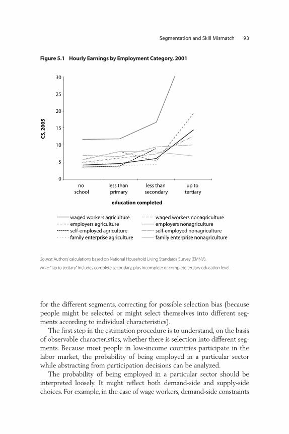
for the different segments, correcting for possible selection bias (becausepeople might be selected or might select themselves into different seg-ments according to individual characteristics).
The first step in the estimation procedure is to understand, on the basisof observable characteristics, whether there is selection into different seg-ments. Because most people in low-income countries participate in thelabor market, the probability of being employed in a particular sectorwhile abstracting from participation decisions can be analyzed.
The probability of being employed in a particular sector should beinterpreted loosely. It might reflect both demand-side and supply-sidechoices. For example, in the case of wage workers, demand-side constraints
Segmentation and Skill Mismatch 93C
S, 2
00
5
30
25
20
15
10
5
0
waged workers agriculture waged workers nonagricultureemployers agriculture employers nonagricultureself-employed agriculture self-employed nonagriculturefamily enterprise agriculture family enterprise nonagriculture
no less than less than up to school primary secondary tertiary
education completed
Figure 5.1 Hourly Earnings by Employment Category, 2001
Source: Authors’calculations based on National Household Living Standards Survey (EMNV).
Note: “Up to tertiary” includes complete secondary, plus incomplete or complete tertiary education level.

might select the people who end up working in that sector. In the case ofmaquila factories, only workers who have completed a secondary educa-tion and are less than 30 years of age can be employed. In the case of theself-employed, employers, and family enterprises, the selection bias ismainly due to the supply side, as they are all independent workers andthey have decided to be employed in that specific sector; however,demand-side forces may still play a role if they are induced to set up andrun their own businesses because they do not find jobs as wage workers.In an analysis of the probability of being employed in a particular sector(formal versus informal; primary, secondary, or tertiary), rather than in aparticular employment category, the explanatory variables used might beinterpreted as reflecting both demand-side and supply-side constraints inthe selection process.
94 Making Work Pay in Nicaragua: Employment, Growth, and Poverty Reduction
agriculture formal secondaryinformal secondary formal tertiaryinformal tertiary
C$
, 20
05
17.5
15.0
12.5
10.0
7.5
5.0
2.5
0 no less than less than up to school primary secondary tertiary
education completed
Figure 5.2 Hourly Earnings by Broad Sector and Informality, 2001
Source: Authors’calculations based on EMNV.
Note: “Up to tertiary” includes complete secondary, plus incomplete or complete tertiary education level.
To estimate how individual and household characteristics affect theprobability of getting a certain job, a multinomial logit model on 2001household survey data is estimated. In the first case, the employment cat-egories are wage workers, employers, and self-employed or family enter-prises, divided into two subcategories: agriculture and nonagriculture.There are six possible alternatives. The category of unemployed and inac-tive people is left out, since the alternative of not working is not feasiblefor most of them except for the youth and for women. In the second case,there are five categories: the primary sector, plus the secondary and terti-ary sectors divided into formal and informal subsectors. For determinatesof earnings, estimates use age, gender, educational attainment, nonlaborincome, regional dummies, and dummies for the presence of the elderly,adults, and children in the household.
The annex contains descriptive statistics of the variables used in theselection and wage equations: on average, employers, the self-employed,and household heads of family enterprises are older than wage workersand have more experience. The majority of agricultural workers aremales, as are the majority of employers (both in and outside of agricul-ture). More than one-third of those working in agriculture are illiterate,and that share increases up to almost 50 percent for the agricultural self-employed and those working in family enterprises. There is a very lowrate of illiteracy among nonagricultural workers (less than 1 percent), and40 percent have at least some primary education. Outside of agriculture,among wage workers and employers, 50 percent have a completed sec-ondary education or above, while only 30 percent of the self-employed orthose working in family enterprises have a completed secondary educa-tion or higher. Agricultural workers are concentrated in the Central andPacific regions, while others work mainly in the Managua region.
Workers in the primary sector are, on average, older and consequentlyhave more experience.5 Males are mostly employed in the primary sector,in the secondary informal sector, and in the tertiary formal sector.Illiterate workers are employed mainly in the primary sector and in theinformal subsector of both the secondary and the tertiary sector. The ter-tiary formal sector comprises mostly workers with a completed second-ary education or above, while the secondary formal sector is evenly divid-ed between workers with incomplete secondary and complete secondaryeducation or above. The good jobs, and the upper tier of the secondaryand tertiary sectors, are concentrated in the Managua region, and peopleworking there have high nonlabor incomes.
Segmentation and Skill Mismatch 95
Table 5.1 illustrates the outcomes of the occupational selectionobtained by estimating a multinomial logit model.6 The reference catego-ry is wage workers in agriculture.7 The table presents the relative risk ratio(RRR), which indicates the likelihood of a worker ending up employed inthe given category (more likely if the coefficient is larger than 1, less like-ly if the coefficient is smaller than 1), compared with being a wage work-er in agriculture, if there is a one-unit increase in the explanatory variable.8
Overall, age, education, region, and nonlabor income significantlyaffect the likelihood of ending up in any given category as compared tobeing a wage worker in agriculture. Higher nonlabor income increases by9 percent the likelihood of ending up as an employer, either outside ofagriculture or in agriculture. It also increases by 9 percent the probabilityof ending up working outside of agriculture as a family enterprise or self-employed. Within agriculture it has no effect on the likelihood of beingself-employed or as a family enterprise. Thus, nonlabor income or assetsmay be acting as a barrier to moving outside of agriculture. Region deter-mines strongly whether a person ends up in an agricultural employmentcategory or not; being outside of Managua reduces the chances of endingup in agriculture. Again, this may suggest barriers to mobility from ruralto urban areas.
Education is an important determinant of being outside of agriculturefor all categories. Within agriculture, more education renders a worker 10percent less likely to work as a family enterprise worker, the lowest earn-ing category. Outside of agriculture, more education increases the likeli-hood of being an employer (by 34 percent), being a wage worker (by 34percent), and being self-employed (by 17 percent). Again, this suggeststhat education might be acting as a barrier to moving to better earningopportunities. Demographic characteristics are in general not significant,except in the case of self-employed or family enterprise workers outsideof agriculture, in which case having more children age six or youngermakes a worker less likely to be in this category.9
Table 5.2 shows the results of selection across the five categoriesdefined by sector of economic activity and informality (primary sector,secondary formal, secondary informal, tertiary formal, and tertiary infor-mal).The reference category is the primary sector.The results indicate thatbeing male decreases the likelihood of working outside of the primary sec-tor. Age increases the likelihood of working in the tertiary sector, but notin the secondary. Education is always significant and increases the likeli-hood of being employed outside of agriculture. The effect of education isslightly higher for the formal sector, with one more year of education
96 Making Work Pay in Nicaragua: Employment, Growth, and Poverty Reduction

Tabl
e 5.
1Se
lect
ion
amon
g Em
ploy
men
t Cat
egor
ies,
200
1
Wag
e w
orke
rsEm
ploy
ers
Self-
empl
oyed
Fam
ily e
nter
prise
s
Non
agric
ultu
reAg
ricul
ture
Non
agric
ultu
reAg
ricul
ture
Non
agric
ultu
reAg
ricul
ture
Non
agric
ultu
re
Varia
bles
RRR
tRR
Rt
RRR
tRR
Rt
RRR
tRR
Rt
RRR
t
Age
1.01
82.
600
1.07
96.
880
1.09
88.
370
1.04
03.
730
1.06
37.
950
1.09
58.
290
1.10
610
.680
Year
s of
edu
catio
n1.
345
10.5
701.
066
1.58
01.
341
8.13
00.
976
–0.7
101.
171
5.57
00.
907
–2.7
901.
126
3.88
0
Gen
der
0.11
4–8
.780
1.95
21.
550
0.36
8–3
.240
0.75
3–0
.870
0.06
3–1
0.77
01.
484
1.08
00.
233
–5.2
40D
umm
y ch
ild a
ge 6
0.86
7–1
.750
0.84
6–1
.310
0.88
9–0
.870
1.07
40.
660
0.93
4–0
.770
0.98
6–0
.150
0.92
7–0
.740
Dum
my
child
7–1
51.
038
0.42
01.
038
0.36
00.
957
–0.4
400.
879
–1.3
900.
993
–0.0
801.
385
3.97
01.
115
1.14
0D
umm
y ad
ult
1.03
70.
630
1.01
90.
240
0.92
4–1
.060
0.83
6–1
.930
0.88
4–2
.070
0.99
6–0
.060
0.91
6–1
.340
Dum
my
elde
rly1.
222
1.04
01.
078
0.26
01.
221
0.69
01.
379
1.16
00.
856
–0.6
900.
827
–0.4
200.
793
–0.7
80N
onla
bor I
ncom
e1.
084
1.98
01.
096
2.24
01.
093
2.18
01.
040
0.89
01.
088
2.06
01.
081
1.92
01.
090
2.12
0Pa
cific
0.29
6–2
.430
1.24
E+08
22.9
900.
545
–1.0
801.
128
0.22
00.
315
–2.1
907.
627
1.89
00.
499
–1.3
60Ce
ntra
l0.
146
–5.2
702.
20E+
0826
.900
0.32
3–2
.590
2.02
71.
880
0.14
4–4
.660
13.8
332.
600
0.32
9–2
.790
Atla
ntic
0.20
7–4
.110
2.24
E+08
24.2
900.
404
–1.8
003.
464
2.98
00.
150
–4.3
0024
.493
3.05
00.
501
–1.7
30
Sour
ce: A
utho
rs’c
alcu
latio
ns b
ased
on
EMN
V.
Not
e: R
RR =
rela
tive
risk
ratio
s, t =
t st
atist
ics.
97
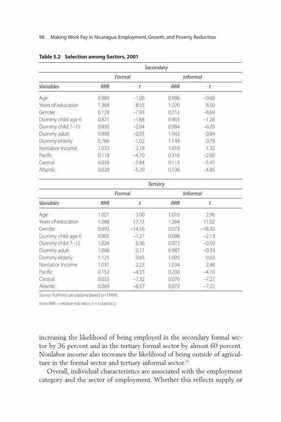
increasing the likelihood of being employed in the secondary formal sec-tor by 36 percent and in the tertiary formal sector by almost 60 percent.Nonlabor income also increases the likelihood of being outside of agricul-ture in the formal sector and tertiary informal sector.10
Overall, individual characteristics are associated with the employmentcategory and the sector of employment. Whether this reflects supply or
98 Making Work Pay in Nicaragua: Employment, Growth, and Poverty Reduction
Table 5.2 Selection among Sectors, 2001
Secondary
Formal Informal
Variables RRR t RRR t
Age 0.989 –1.06 0.996 –0.60Years of education 1.364 8.55 1.220 8.50Gender 0.128 –7.93 0.212 –8.69Dummy child age 6 0.871 –1.68 0.903 –1.28Dummy child 7–15 0.850 –2.04 0.984 –0.25Dummy adult 0.998 –0.03 1.043 0.84Dummy elderly 0.766 –1.02 1.144 0.79Nonlabor Income 1.032 2.18 1.019 1.32Pacific 0.118 –4.70 0.316 –2.60Central 0.039 –7.64 0.113 –5.47Atlantic 0.020 –5.29 0.106 –4.85
Tertiary
Formal Informal
Variables RRR t RRR t
Age 1.021 3.00 1.016 2.96Years of education 1.588 17.13 1.264 11.02Gender 0.093 –14.56 0.073 –18.30Dummy child age 6 0.905 –1.27 0.886 –2.13Dummy child 7–15 1.026 0.36 0.973 –0.50Dummy adult 1.006 0.11 0.987 –0.33Dummy elderly 1.125 0.65 1.005 0.03Nonlabor Income 1.031 2.23 1.034 2.48Pacific 0.152 –4.55 0.200 –4.10Central 0.053 –7.32 0.076 –7.27Atlantic 0.069 –6.57 0.072 –7.22
Source: Authors’calculations based on EMNV.
Note: RRR = relative risk ratios, t = t statistics.
demand conditions, or both, is not possible to infer from the analysis pre-sented here. Education, nonlabor income, and region seem to play a keyrole in this selection process, increasing the chances of ending up in bet-ter-earning jobs. As such, if one is going to further explore barriers tomobility, these present themselves as good candidates for analysis.
After controlling for selection bias, the analysis of the determinants ofearnings differentials across segments of the labor markets comes into thepicture. The annex presents the results of estimated earnings equations.11
Age increases earnings for wage workers and for household enterpriseworkers in agriculture, and being outside of Managua reduces these earn-ings. Education increases returns outside of agriculture for wage workers,employers, and self-employed but has no effect on household enterpriseworkers. Within agriculture, education increases the income of wageworkers and self-employed workers. It is important to note that incomefor family enterprises is calculated as the profits from the enterprisedivided by the number of workers in the household; as such, it capturesthe returns to all factors of production, rather than to individual factorsof production. So caution is needed when interpreting the results of earn-ings equations for this group. In particular, the lack of effect of educationon household enterprise workers might just reflect this fact, rather thanno effect at all.12 The premium for education is higher outside of agricul-ture and in the formal sector of the economy.13 The above results areimportant for educational policy for two reasons: one, education may beacting as a barrier to mobility, and two, education may increase earningsin some low-earning sectors and categories.
In order to determine whether there are wage differentials across labormarket segments, the Oaxaca-Blinder decomposition is performed. (It isexplained in equation 5.1, where the term lnϖj – lnϖs corresponds toearnings gap net of selectivity effects.) The results allow identification of(i) whether the observed net wage differentials are statistically significant,and (ii) which part of the wage differentials between labor market seg-ments can be attributed to differences in average individual characteris-tics and which can be attributed to returns to observed characteristics(represented as total, endowments, and β coefficients, respectively, intable 5.3 and table 5.4).
The results indicate that there are significant wage differentialsbetween the primary and the secondary/tertiary sectors, with most of thedifference explained by differences in returns to individual characteristics(table 5.3). In all cases, differences in returns to individual characteristics
Segmentation and Skill Mismatch 99

100 Making Work Pay in Nicaragua: Employment, Growth, and Poverty Reduction
Table 5.3 Oaxaca-Blinder Decomposition by Employment Category
Coefficient P -value
Wage worker nonagriculture vs. wage worker agriculture Net difference 0.342 0.445 Endowments 0.517 0.093ß coefficients –0.336 0.480Interaction 0.160 0.617
Wage worker nonagriculture vs. enterprise agricultureNet difference 4.083 0.259Endowments –0.364 0.006ß coefficients 5.715 0.348Interaction –1.268 0.717
Wage worker nonagriculture vs. employers nonagricultureNet difference 4.409 0.001Endowments 0.248 0.000ß coefficients 4.813 0.002Interaction –0.652 0.004
Wage worker nonagriculture vs. self-employed agricultureNet difference 0.914 0.289Endowments 0.713 0.297ß coefficients 0.312 0.724Interaction –0.111 0.873
Wage worker nonagriculture vs. self-employed nonagricultureNet difference 1.122 0.001Endowments –0.255 0.000ß coefficients 1.425 0.000Interaction –0.048 0.580
Wage worker nonagriculture vs. family enterprise worker in agricultureNet difference 0.703 0.130Endowments –0.494 0.002ß coefficients 1.718 0.116Interaction –0.521 0.461Wage worker nonagriculture vs. family enterprise worker nonagricultureNet difference 0.127 0.909Endowments 0.045 0.853ß coefficients –0.102 0.928Interaction 0.184 0.497
Source: Authors’calculations based on EMNV.

explain most of the differential.14 In looking at which characteristics areresponsible for these differences in returns, it is age, education, and regionthat account for an important part of the difference, meaning that thereis a higher premium for education and experience outside of agriculture,with the premium lower in the Central and Atlantic regions. Wage differ-entials, however, are not significant between formal and informal sectors.Formal and informal sectors have significantly different compositions ofthe labor force, but returns to individual characteristics are not signifi-cantly different.
Table 5.4 shows the results among employment categories. The refer-ence category is wage employment outside of agriculture. Earnings differ-entials—net of selection effects—are only significant between wage work-ers and self-employed outside of agriculture and between wage workers
Segmentation and Skill Mismatch 101
Table 5.4 Oaxaca-Blinder Decomposition by Employment Sector
Coefficient P-value
Secondary informal vs. primaryNet difference 1.326 0.083Endowments –0.648 0.150ß coefficients 1.205 0.110Interaction 0.769 0.090
Tertiary informal vs. primaryNet difference 1.234 0.018Endowments –0.922 0.170ß coefficients 1.065 0.058Interaction 1.092 0.108
Secondary formal vs. secondary informalNet difference 1.598 0.171Endowments –0.341 0.002ß coefficients 1.773 0.135Interaction 0.167 0.174
Tertiary formal vs. tertiary informalNet difference 0.110 0.856Endowments –0.778 0.002ß coefficients 0.398 0.512Interaction 0.490 0.049
Source: Authors’calculations based on EMNV.
and employers outside of agriculture. In both cases, net earnings differen-tials are positive, while observed earnings differentials are negative. Thismeans that selection is playing an important role in observed differencein average earnings among these categories. In both cases the net earningspremium is positive for wage workers owing to higher returns to individ-ual endowments, with age and education having the most importanteffect (see annex). Net earnings differentials are not significant betweenother employment categories and wage workers outside of agriculture,which means that differences in observed earnings arise solely because ofselection effects.
Thus, there appears to be segmentation between the primary and sec-ondary/tertiary sectors, or in other words, between employment in agri-culture and nonagriculture. Potential segmentation between the formaland the informal is not supported by the results. Potential segmentationbetween wage workers and self-employed workers and between wageworkers and employers outside of agriculture is also supported by theresults. Differences in earnings between other employment categoriesarise mostly as a result of selection, whereby more educated and olderworkers select themselves or are selected into higher-earning employ-ment options.
Evidence from section A suggests that selection into employment out-side of agriculture plays an important role in explaining observed earn-ings, with education playing the most prominent role in this selectionprocess. Even after a netting out of the effects of selection from the nona-gricultural earnings premium, there is an important premium to workingoutside of agriculture, with most of the difference being explained by dif-ferences in returns to endowments, mainly age, education, and location.Therefore, some potential segmentation between agricultural and non-agricultural employment is supported by the data. Potential segmentationbetween formal and informal work is not supported by the data. Instead,selection effects appear to explain the observed earnings differentials.Selection into formal employment is determined mostly by educationand gender, with more education and being a male increasing the chancesof selecting or being selected into formal employment.
In terms of employment categories, the results suggest that most of theobserved earnings differentials can be attributed to selection effects. Oncethese effects are controlled for, there are no significant differences amongmost of the employment categories, except for earnings premium in wagework and self-employment outside of agriculture. Selection into better-
102 Making Work Pay in Nicaragua: Employment, Growth, and Poverty Reduction
earning employment categories is determined by education, age, and non-labor income. Nonlabor income appears to be an important determinantfor being an employer, which may be an indication of credit constraints,as those with other sources of income may also be able to offer more ascollateral.
Thus, in terms of policy it is important to understand the barriers toselection into formal employment and wage work and to moving peopleoutside of agriculture. In addition, credit constraints to becoming anemployer merit further research.
As has been mentioned, however, differences in returns to individualcharacteristics among segments of the labor market are only a first step inidentifying segmentation. These differences may be capturing other non-pecuniary characteristics of jobs (such as flexibility or regional price dif-ferences), which are not explored here. In addition, the differences areinconclusive about whether workers end up in a given segment becauseof choice or through lack of an alternative. These issues are explored fur-ther in section B.
Segmentation and Barriers to Mobility: A Qualitative Approach
The previous section showed that when controlling for observable char-acteristics, markets may be segmented between agriculture and nonagri-culture, among formal and informal secondary sectors, and amongemployers and nonemployers.
However, this is not sufficient for an understanding of whether there issegmentation among good and bad job sectors. For segmentation to bepresent, it is necessary that workers not be in the low-paying alternativesthrough choice. Unfortunately, this is a question that is rarely addressed inhousehold surveys. However, the Nicaragua household survey contains aquestion that addresses this issue for the nonagricultural self-employed. Inparticular, the 2001 survey includes a question that may help to identifywhether the nonagricultural self-employed are self-employed becausethey cannot find a wage job. Those who respond as being self-employed inthe nonagricultural sector are asked detailed questions about the type ofbusiness they have. Among these questions they are asked the reason foropening a business. One possible answer is “because [they] could not findwage employment.” In other words, they would rather be wage workers.
Table 5.5 summarizes evidence from the survey question reportedabove, disaggregating the results by level of education, and table 5.6 sum-
Segmentation and Skill Mismatch 103

marizes the same evidence by poverty level. For the population as awhole, the main reason for starting a business is because it gives workersmore flexibility, and this is followed by wanting to complement othersources of income.
However, when the answer is disaggregated by level of education, it isfound that for those with no schooling or with incomplete primary edu-cation, the most important reason for starting a business is to comple-ment other sources of income, followed by the inability to find wageemployment. It should also be noted that a very low proportion of low-skilled workers answer that they started a business because they couldhave a higher income than as a wage worker. Thus, self-employment doesseem to be a last-resort option for 23 percent of those with low skills.
When the results are disaggregated by poverty level a similar pictureemerges. Twenty-six percent of the poor started a business because theywere unable to find wage employment. However, 28 percent did sobecause of the flexibility it allowed them. Only 3 percent started a busi-ness because they believed that they could have higher earnings than aswage workers.
This suggests that some sort of segmentation may be occurring for thosewith very low skills, which is consistent with the evidence in section A.
104 Making Work Pay in Nicaragua: Employment, Growth, and Poverty Reduction
Table 5.5 Reason for Starting a Business, by Level of Education, 2001(percentage who state as main reason)
No Incomplete Complete Incomplete Complete Schooling Primary Primary Secondary Secondary Tertiary All
Implied flexibilitya 23 32 39 36 35 35 33Get higher income 4 5 6 11 10 12 7
than as wage employment
Complement other income 35 37 25 26 32 21 31
Could not find wage 23 17 20 17 18 12 18employment
Wanted to use skills 2 1 1 4 1 10 2Other 13 9 9 5 5 11 9Total 100 100 100 100 100 100 100
Source: Authors’calculations based on EMNV.
a. “Implied flexibility”aggregates the following answers: “wanted to be independent,”“flexible time,”and “combinework and households activities.”
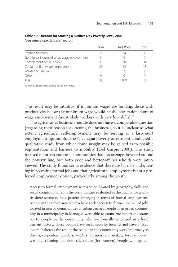
The result may be intuitive: if minimum wages are binding, those withproductivity below the minimum wage would be the ones rationed out ofwage employment (most likely workers with very low skills).15
The agricultural business module does not have a comparable question(regarding their reason for opening the business), so it is unclear to whatextent agricultural self-employment may be serving as a last-resortemployment option. But the Nicaragua poverty assessment conducted aqualitative study from which some insight may be gained as to possiblesegmentation and barriers to mobility (Del Carpio 2006). The studyfocused on urban and rural communities that, on average, hovered aroundthe poverty line, but both poor and better-off households were inter-viewed. The study found some evidence that there are barriers and queu-ing in accessing formal jobs and that agricultural employment is not a pre-ferred employment option, particularly among the youth.
Access to formal employment seems to be limited by geography, skills andsocial connections. From the communities evaluated in the qualitative analy-sis there seems to be a pattern emerging in terms of formal employment;people in the urban area tend to have wider access to formal low skilled jobslocated in nearby communities or urban centers. People in an urban commu-nity in a municipality in Managua were able to count and report the statuson 10 people in the community who are formally employed in a localcement factory. Those people have social security benefits and have a fixedincome whereas the rest of the people in the community work informally asdrivers, carpenters, builders, welders (all men) and making tortillas, bread,washing, cleaning and domestic duties (for women) People who gained
Segmentation and Skill Mismatch 105
Table 5.6 Reason for Starting a Business, by Poverty Level, 2001(percentage who state each reason)
Poor Not Poor Total
Implied flexibility 28 34 33Get higher income than as wage employment 3 9 7Complement other income 33 30 31Could not find wage employment 26 15 18Wanted to use skills 1 3 2Other 9 9 9Total 100 100 100
Source: Authors’calculations based on EMNV.

employment in the cement factory or maquilas usually have someonealready working who helped them gain employment; the majority of thepeople however cannot access these jobs because they either lack the skillsnecessary, a connection or both. In RAAS [the Autonomous Region of theAtlantic South], the ability to speak English is a necessary skill to work as anembarcado (in cruise ship); people with low levels of education, ability tospeak English and an initial fee for paperwork (passport, medical exams,etc.) can access these jobs. In Managua, a high school degree is required towork in the maquila factories; age (under 30) is also a factor that some ofthe youth mention is a requirement. People in some rural communitiesexhibited frustration toward the lack of employment outside of agriculture;many are hopeful about the prospect of finding a job, particularly the youthwho often aspire to work in an activity different than that of their father(agriculture).There is wide heterogeneity in economic functions and oppor-tunities related to agriculture; disparities within communities and betweenthem as well as gender divisions. Livestock and commerce of livestock prod-ucts (milk, cuajada, meat) are generally reserved for the more affluent mem-bers of the community.31 (Del Carpio 2006, 5).
In addition, the sector of employment was perceived by the inter-viewed communities, together with the available services and education-al attainment, as important factors in determining the socioeconomicchange. The youth in particular expressed their concern for the lack ofadequate employment opportunities and for the little access they have tovocational training; they see agricultural work as the only available occu-pation. They want to have a better life than their parents and would liketo have a profession but see no alternatives, no one has come to help themor worry about them” (Del Carpio 2006, 22).
Throughout the qualitative analysis, a rural-urban divide was present.Rural communities have more limited access to nonfarm employmentand to education. Both factors reinforce each other and act as barriers forthe poor in moving out of poverty through better employment opportu-nities. Although communities perceive education to be important foraccessing better earning opportunities, the qualitative evidence is that thesupply of educational services is vastly reduced in rural areas, and partic-ularly in remote ones. The transport costs for accessing secondary educa-tion are high, and in the winter months the lack of infrastructure makesit impossible for children and teachers to reach schools. In one of the ruralcommunities interviewed, parents do not send their daughters to school
106 Making Work Pay in Nicaragua: Employment, Growth, and Poverty Reduction

because they perceive their daughters to be at risk, given the long dis-tances that they must travel.
All of the above factors suggest that rural farm employment may be anonpreferred sector of employment, and that skill and geographic barri-ers reduce outward mobility for this sector. Formal wage employment, onthe other hand, seems to be an option mostly for urban workers.Although many opt for self-employment as a choice rather than as a last-resort option, an important fraction, particularly those with low skills,prefer self-employment to wage employment. Queuing is evidenced bythe need for connections in accessing formal wage employment. Finally,lack of skills seems to be a major obstacle to good employment opportu-nities. The next section explores the skill mismatch in more detail.
Skill Mismatch
As mentioned at the beginning of this chapter, in noncompetitive settings,supply and demand may not equate to “clear the market.” Instead, mar-ket imperfections and friction may imply that a share of those needingemployment end up unemployed or, if unemployment is not an option,in the bad jobs sector. This means that markets would be segmented inthe sense defined in section B; that is, two agents with similar character-istics would end up with different earnings depending on their segmentof the labor market (in the good jobs sector versus unemployed or in thebad jobs sector).
However, although segmentation implies that there may be two iden-tical individuals with different earnings because they are in different seg-ments, it is also well known that the compositions of labor market seg-ments differ, with the good jobs sector having a lower share of unskilledworkers than the unemployed sector and the bad jobs sector. A possibleexplanation is that the rigidities that generate the segmentation are morebinding for the unskilled. For example, minimum wages or union-setwages affect the unskilled more than the skilled. If workers in the bad jobssector could become skilled, they would have a higher probability ofbeing hired in the good jobs sector. In terms of demand and supply, thismeans that excess supply is higher for the unskilled population. This iswhat is referred to as mismatch of skills.
Skill mismatch matters not only in a static sense but also and probablymost importantly, in a dynamic sense. In the presence of skill-biased tech-nical change, skill mismatch is likely to increase. The larger the share of
Segmentation and Skill Mismatch 107
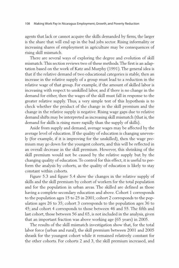
agents that lack or cannot acquire the skills demanded by firms, the largeris the share that will end up in the bad jobs sector. Rising informality orincreasing shares of employment in agriculture may be consequences ofrising skill mismatch.
There are several ways of exploring the degree and evolution of skillmismatch.This section reviews two of these methods.The first is an adap-tation based on the work of Katz and Murphy (1991). The general idea isthat if the relative demand of two educational categories is stable, then anincrease in the relative supply of a group must lead to a reduction in therelative wage of that group. For example, if the amount of skilled labor isincreasing with respect to unskilled labor, and if there is no change in thedemand for either, then the wages of the skill must fall in response to thegreater relative supply. Thus, a very simple test of this hypothesis is tocheck whether the product of the change in the skill premium and thechange in the relative supply is negative. Rising wage gaps due to relativedemand shifts may be interpreted as increasing skill mismatch (that is, thedemand for skills is rising more rapidly than the supply of skills).
Aside from supply and demand, average wages may be affected by theaverage level of education. If the quality of education is changing uneven-ly (for example, if it is improving for the unskilled), then the wage pre-mium may go down for the youngest cohorts, and this will be reflected inan overall decrease in the skill premium. However, this shrinking of theskill premium would not be caused by the relative supply but by thechanging quality of education.To control for this effect, it is useful to per-form the analysis by cohorts, as the quality of education is likely to stayconstant within cohorts.
Figure 5.3 and figure 5.4 show the changes in the relative supply ofskills and the skill premium by cohort of workers for the total populationand for the population in urban areas. The skilled are defined as thosehaving a complete secondary education and above. Cohort 1 correspondsto the population ages 15 to 25 in 2001; cohort 2 corresponds to the pop-ulation ages 26 to 35; cohort 3 corresponds to the population ages 36 to45; and cohort 4 corresponds to those between 46 and 55. The fifth andlast cohort, those between 56 and 65, is not included in the analysis, giventhat an important fraction was above working age (65 years) in 2005.
The results of the skill mismatch investigation show that, for the totallabor force (urban and rural), the skill premium between 2001 and 2005shrank for the youngest cohort while it remained relatively constant forthe other cohorts. For cohorts 2 and 3, the skill premium increased, and
108 Making Work Pay in Nicaragua: Employment, Growth, and Poverty Reduction
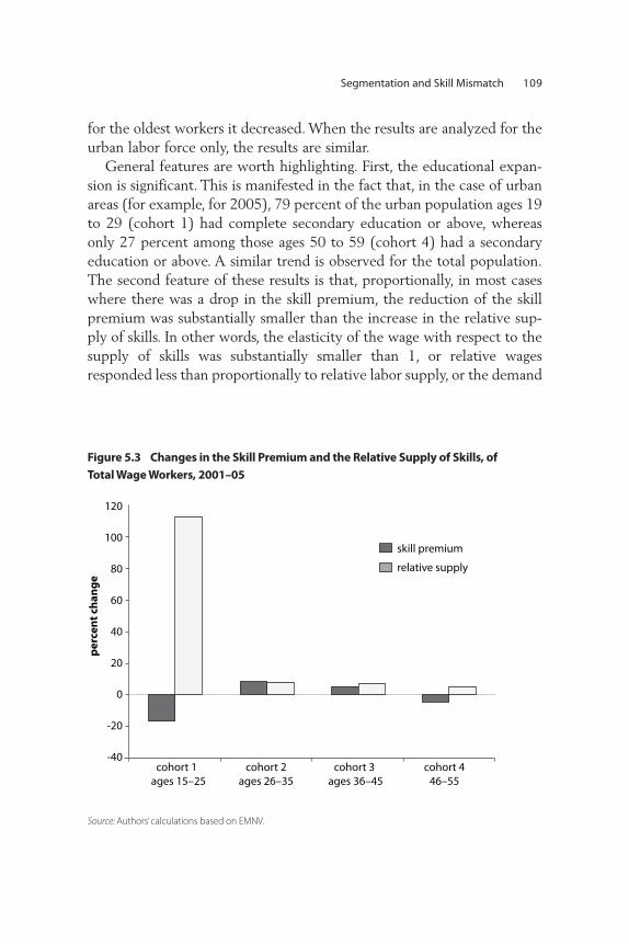
Segmentation and Skill Mismatch 109p
erce
nt
chan
ge
120
100
80
60
40
20
0
-20
-40 cohort 1 cohort 2 cohort 3 cohort 4 ages 15–25 ages 26–35 ages 36–45 46–55
skill premium
relative supply
Figure 5.3 Changes in the Skill Premium and the Relative Supply of Skills, of Total Wage Workers, 2001–05
Source: Authors’calculations based on EMNV.
for the oldest workers it decreased. When the results are analyzed for theurban labor force only, the results are similar.
General features are worth highlighting. First, the educational expan-sion is significant. This is manifested in the fact that, in the case of urbanareas (for example, for 2005), 79 percent of the urban population ages 19to 29 (cohort 1) had complete secondary education or above, whereasonly 27 percent among those ages 50 to 59 (cohort 4) had a secondaryeducation or above. A similar trend is observed for the total population.The second feature of these results is that, proportionally, in most caseswhere there was a drop in the skill premium, the reduction of the skillpremium was substantially smaller than the increase in the relative sup-ply of skills. In other words, the elasticity of the wage with respect to thesupply of skills was substantially smaller than 1, or relative wagesresponded less than proportionally to relative labor supply, or the demand

for skills was increasing for the period analyzed. Third, it is worth high-lighting that the skill premium is lower in the younger cohorts, where therelative supply of skills is highest, which reinforces the idea that the high-er supply of skills is reducing its relative return.
The above analysis suggests that the demand for skills in the wage sec-tor is increasing. In the case of cohorts 2 and 3, the evidence suggests thatthe supply of skills, although increasing slightly, is increasing at a slowerpace than the relative demand. For the oldest cohort (4) the result is theopposite. In the younger cohorts, however, the increase in the supply oflabor was large enough to have had a downward impact on the relativewage. This may imply that, as the educational expansion continues, thewage differential could possibly be further reduced. The implications forpoverty reduction will depend on whether this contraction of the skill
110 Making Work Pay in Nicaragua: Employment, Growth, and Poverty Reductionp
erce
nt
chan
ge
140
120
100
80
60
40
20
0
-20
-40 cohort 1 cohort 2 cohort 3 cohort 4 ages 15–25 ages 26–35 ages 36–45 46–55
skill premium
relative supply
Figure 5.4 Changes in the Skill Premium and the Relative Supply of Skills, of Urban Wage Workers, 2001–05
Source: Authors’calculations based on EMNV.
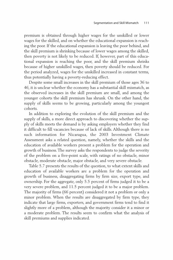
premium is obtained through higher wages for the unskilled or lowerwages for the skilled, and on whether the educational expansion is reach-ing the poor. If the educational expansion is leaving the poor behind, andthe skill premium is shrinking because of lower wages among the skilled,then poverty is not likely to be reduced. If, however, part of this educa-tional expansion is reaching the poor, and the skill premium shrinksbecause of higher unskilled wages, then poverty should be reduced. Forthe period analyzed, wages for the unskilled increased in constant terms,thus potentially having a poverty-reducing effect.
Despite some small increases in the skill premium of those ages 36 to46, it is unclear whether the economy has a substantial skill mismatch, asthe observed increases in the skill premium are small, and among theyounger cohorts the skill premium has shrunk. On the other hand, thesupply of skills seems to be growing, particularly among the youngestcohorts.
In addition to exploring the evolution of the skill premium and thesupply of skills, a more direct approach to discovering whether the sup-ply of skills meets the demand is by asking employers whether they findit difficult to fill vacancies because of lack of skills. Although there is nosuch information for Nicaragua, the 2003 Investment ClimateAssessment asks a related question, namely, whether the skills and theeducation of available workers present a problem for the operation andgrowth of business. The survey asks the respondents to judge the severityof the problem on a five-point scale, with ratings of no obstacle, minorobstacle, moderate obstacle, major obstacle, and very severe obstacle.
Table 5.7 presents the results of the question, to what extent skills andeducation of available workers are a problem for the operation andgrowth of business, disaggregating firms by firm size, export type, andownership. For the aggregate, only 5.5 percent of firms judged it to be avery severe problem, and 11.5 percent judged it to be a major problem.The majority of firms (66 percent) considered it not a problem or only aminor problem. When the results are disaggregated by firm type, theyindicate that large firms, exporters, and government firms tend to find itslightly more of a problem, although the majority consider it a minor ora moderate problem. The results seem to confirm what the analysis ofskill premiums and supplies indicated.
Segmentation and Skill Mismatch 111
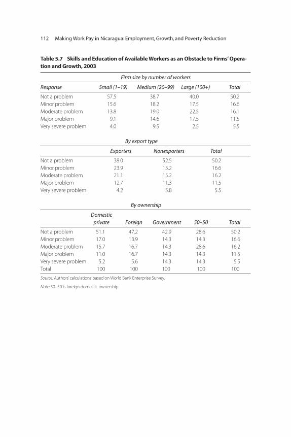
112 Making Work Pay in Nicaragua: Employment, Growth, and Poverty Reduction
Table 5.7 Skills and Education of Available Workers as an Obstacle to Firms’ Opera-tion and Growth, 2003
Firm size by number of workers
Response Small (1–19) Medium (20–99) Large (100+) Total
Not a problem 57.5 38.7 40.0 50.2Minor problem 15.6 18.2 17.5 16.6Moderate problem 13.8 19.0 22.5 16.1Major problem 9.1 14.6 17.5 11.5Very severe problem 4.0 9.5 2.5 5.5
By export type
Exporters Nonexporters Total
Not a problem 38.0 52.5 50.2Minor problem 23.9 15.2 16.6Moderate problem 21.1 15.2 16.2Major problem 12.7 11.3 11.5Very severe problem 4.2 5.8 5.5
By ownership
Domestic private Foreign Government 50–50 Total
Not a problem 51.1 47.2 42.9 28.6 50.2Minor problem 17.0 13.9 14.3 14.3 16.6Moderate problem 15.7 16.7 14.3 28.6 16.2Major problem 11.0 16.7 14.3 14.3 11.5Very severe problem 5.2 5.6 14.3 14.3 5.5Total 100 100 100 100 100
Source: Authors’calculations based on World Bank Enterprise Survey.
Note: 50–50 is foreign domestic ownership.
Notes
1. Labor market segmentation is now part of the standard labor economic text-books; see, for example, Borjas (1996), Bosworth, Dawkins, and Stromback(1996), and Layard, Nickell, and Jackson (1991). The main reason is that itoffers a better explanation for some empirical observations than the compet-itive model. An often-quoted example is the persistent existence of intrain-dustry wage differentials for observationally equivalent workers (Katz andSummers 1988). For other contributions, see Dickens and Lang (1985) andEsfahani and Salehi-Isfahani (1989).
2. The bad jobs sector is usually associated with the agricultural sector or theinformal sector, and the good jobs sector is generally associated with theindustrial or modern sector or the formal sector.This distinction may oversim-plify; the division of the labor market between good and bad jobs goes beyondthe formal versus informal or agricultural versus industrial divides anddepends on the specificities of each country.
3. See Newman and Oaxaca (2004) for a discussion of earning gap decomposi-tion in the presence of selection.
4. The graph does not show earnings for family enterprises and self-employed inagriculture for workers with complete secondary or more because there werevery few observations in each cell.
5. Experience is constructed as age minus years of education minus six.
6. It is a generalization of the two-step selection-bias correction method intro-duced by Heckman (1979) that allows for any parameterized error distribu-tion. It only requires the estimation of one parameter in the correction termthat is achieved at the cost of some restrictive assumptions, namely, linearityin the outcome variable and joint normality in the error terms (seeBourguignon, Fournier, and Gurgand 2007).
7. The analysis has left out the no-education dummy and the Managua dummyto avoid perfect collinearity.
8. Relative risk ratios (RRRs) are presented as an exponential; thus a coefficientlower than 1 indicates a negative effect and a coefficient larger than 1 indi-cates a positive effect. For example, the first column in the table indicates thatan increase of one year in age makes a worker 1.02 times more likely to endup employed as a wage worker outside of agriculture than to end upemployed as a wage worker in agriculture.
9. Some of the results suggest that a sequential decision might be taking place.However, this possibility was examined by testing IIA assumptions. In all butone case IIA assumptions held, so further nested models were explored.
Segmentation and Skill Mismatch 113
10. Caution should be exercised in inferring causality; it might be that because aworker is outside of agriculture the worker’s nonlabor income is higher, ratherthan the other way around.
11. Earnings functions are separately estimated for the two classificationsdescribed above. The dependent variable is the logarithm of hourly earnings;the impact of estimated coefficients is measured in terms of percentagechange in hourly earnings for a unit increase in the explanatory variable. Sincean analysis controls for selection bias by using a number of variables that canbe interpreted as demand- and supply-side constraints, only standard controlsother than the selection term λ are included in the wage equations.
12. There are other approaches to calculating returns to labor for householdenterprise workers. One approach is to estimate a profit function, with differ-ent types of labor forces—female adult, female young, male adult, maleyoung—in efficiency units (that is, adjusted by years of education of each),and then impute returns to labor to each type of worker. Alternatively, insteadof using as regressors the head of the enterprise’s individual characteristics,one might use the average characteristics of the household.
13. Again the lack of returns to education in agriculture overall may reflect thefact that household enterprise workers are almost 50 percent of all workers inthis sector.
14. For a more detailed analysis, the tables in the annex report Oaxaca-Blinderdecompositions for each variable.
15. The analysis assumes that more-skilled workers are more productive, and thatin the medium and long run, diminishing marginal returns to labor due tofixed capital need not set in. If in fact capital is fixed, then the marginal prod-uct of labor will also depend on the employment decisions of the firm (thatis, how many workers to hire).
114 Making Work Pay in Nicaragua: Employment, Growth, and Poverty Reduction

Despite modest economic growth and important employment growth,Nicaragua saw no major decrease in poverty. Two main factors explainthis outcome. One, an important fraction (39 percent) of new jobs wasgenerated in agriculture, which offers the lowest returns among econom-ic activities. Two, jobs with good earnings, generated outside of agricul-ture, either were accessible only to the most educated workers, as in thecase of the maquila sector, or experienced a decrease in wages, as was thecase for the industrial food and beverage sector.
The depth of poverty, as measured by the poverty gap, saw significantreductions. These reductions in poverty were due to the following:increases in the relative prices of products produced by the agriculturalpoor, and an increase in the amount of remittances. However, the increasein income was not sufficient to bring the poorest out of poverty.
The analysis presented here has implications for action on five policyfronts: (i) skills, (ii) productivity, (iii) employment generation, (iv) geo-graphic mobility, and (v) regulation of minimum wage.
Skill levels in Nicaragua are substantially lower than in neighboringcountries. Despite the important progress on this front, substantial efforts
C H A P T E R 6
Policy Implications and Further Research
115
are still needed. Increasing skills in Nicaragua would involve both bene-fits and risks, and any education policy must try to magnify the formerwhile minimizing the latter. Currently, the supply of skills seems to begrowing at a higher rate than the demand, and, as a consequence, wagesfor the skilled population might drop. Such a drop in the returns toschooling could serve as a disincentive to acquiring education and mightreduce employment growth in the waged sectors of the economy, main-ly manufacturing and services. It is thus imperative that policies toincrease growth in these sectors (and with this, to increase the demandfor labor) be undertaken.
Currently, constraints to growth appear to lie outside of the labor mar-ket and involve macroeconomic uncertainty and lack of affordable cred-it. An increase in the demand for wage work and, in particular, for higherskills is unlikely to be seen unless these constraints are addressed.However, higher skills are important determinants of earnings among theurban self-employed and family enterprises, as well as among urban infor-mal wage workers. Higher skills are also important in increasing earningsin wage agricultural work and among agricultural employers. Targetingthe expansion of education to the rural sector appears to have importantpotential as a poverty-reducing strategy. Education is a key determinantin accessing better earning opportunities and in moving out of agriculture.
Productivity in Nicaragua declined during the period studied, withimportant decreases within agriculture. Nicaragua has the lowest levels ofagricultural productivity among its neighbors and trading partners. Thisfactor, together with some indirect evidence of low mobility betweenurban and rural areas, suggests that raising productivity in agricultureshould also be in the forefront of policy initiatives. Without targetedinvestments in agricultural productivity and agricultural exports, decreas-ing rural poverty in the short and medium runs seems implausible.
Employment generation should be targeted toward the formal second-ary and tertiary unskilled labor–intensive sectors. Exploring targetedinterventions to foster growth in such sectors as tourism, with trainingprograms for the unskilled specifically designed for the industry, seems apolicy worth exploring. Nicaragua recently conducted a tourism invest-ment climate survey that may provide initial input for the design of thispolicy. Regulation does not seem to pose a constraint for job creation andgrowth. The most urgent policies in this area would seem to be to addressmacroeconomic uncertainty and credit constraints.
116 Making Work Pay in Nicaragua: Employment, Growth, and Poverty Reduction
The study pointed toward possible geographical barriers to mobilitybetween the urban and the rural sectors. It is as yet unclear how impor-tant these barriers to mobility are, and what the main determinants of thebarriers are. Further study on this issue may yield promising policy impli-cations. Becoming an employer is also linked with availability of nonlaborincome, which leads to the natural question of whether alleviating creditconstraints might help more family enterprise workers or self–employedto become employers.
It is unclear to what extent the current minimum wage structure inNicaragua provides any benefits or manages to take into account the skillsof the labor force. More productive sectors have higher minimum wagesand thus may be constraining the poorest from accessing jobs in precise-ly the sectors that offer the highest earnings potential. Workers with pro-ductivity below the minimum wage will be rationed out of formalemployment. The higher the minimum wage is, the less access theunskilled have to these sectors. Results of this study suggest that mini-mum wages may be binding for the maquila manufacturing sector andprobably for commerce. Further study in this area may clarify the extentto which the current sectoral structure of minimum wages is beneficial tothe poor or is actually constraining them from accessing jobs in the mostproductive sectors of the economy.
Policy Implementations and Further Research 117


Arias, Omar, Andreas Blom, Mariano Bosch, Wendy Cunningham, Ariel Fiszbein,Gladys López Acevedo, William Maloney, Jaime Saavedra, Carolina Sánchez-Páramo, Mauricio Santamaría, and Lucas Siga. 2005. “Pending Issues inProtection, Productivity Growth, and Poverty Reduction.” Policy ResearchWorking Paper No. 3799, World Bank, Washington, DC.
Besley, Timothy, and Robin Burgess. 2004. “Can Labor Regulation HinderEconomic Performance? Evidence from India.” Quarterly Journal of Economics119 (1): 91–132.
Bibi, Sami. 2005. “When Is Economic Growth Pro-Poor? Evidence from Tunisia.”Paper presented at the Economic Research Forum, 12th Annual Conference,Cairo, Egypt, December 19–21, 2005.
Borjas, G. J. 1996. Labor Economics. New York: McGraw-Hill.
Bosworth, D., P. Dawkins, and T. Stromback. 1996. The Economics of the LaborMarket. Essex, England: Addison Wesley Longman, Ltd.
Bourguignon, François. 2002. “The Growth Elasticity of Poverty Reduction:Explaining Heterogeneity across Countries and Time Periods.” DELTAWorking Papers No. 2002–03. Département et Laboratoire d'EconomieThéorique et Appliquée of the École Normale Supérieure, Paris, France.
References
119

Bourguignon, François, and Gary S. Fields. 1997. “Discontinuous Losses fromPoverty, Generalized P· Measures, and Optimal Transfers to the Poor.” Journalof Public Economics 63 (2): 155–75.
Bourguignon, F., M. Fournier, and M. Gurgand. 2007. “Selection Bias CorrectionsBased on the Multinomial Logit Model: Monte Carlo Simulations.” Journal ofEconomic Surveys.” 21 (1): 174–205.
Calderón, César, and Alberto Chong. 2005. “Are Labor Market Regulations anObstacle for Long Run Growth?” In Labor Markets and Institutions, ed. J. E.Restrepo and A. Tokman. Santiago, Chile: Banco Central de Chile.
Chen, Shaohua, and Martin Ravallion. 2004. “How Have the World’s Poor Faredsince the Early 1980’s.” World Bank Research Observer 19: 141–69.
Contreras, Dante. 2001. “Economic Growth and Poverty Reduction by Region:Chile 1990–1996.” Development Poverty Review 19 (3): 291–302.
Cukierman, Alex, Martin Rama, and Jan van Ours. 2001. “Long-Run Growth, theMinimum Wage and Other Labor Market Institutions. Preliminary notes.”Mimeo. World Bank, Washington, DC. http://www.tau.ac.il/~alexcuk/pdf/GrowthB.pdf .
Datt, Gaurav, and Martin Ravallion. 1993. “Growth and RedistributionComponents of Changes in Poverty Measures: A Decomposition withApplications to Brazil and India in the 1980s.” Journal of DevelopmentEconomics 38: 275–95.
———. 1998. “Farm Productivity and Rural Poverty in India.” Journal ofDevelopment Studies 24 (4): 62–85.
Del Carpio, Ximena. 2006. “Voices of Nicaragua. A Qualitative and QuantitativeApproach to Viewing Poverty in Nicaragua.” Mimeo, World Bank,Washington, DC.
Dickens, W. T., and K. Lang. 1985. “Testing Dual Labor Market Theory:Reconsideration of the Evidence.” NBER Working Paper Series No. 1670,1–27. National Bureau of Economic Research, Cambridge, MA.
Dollar, David, and Aart Kraay. 2002. “Growth Is Good for the Poor.” Journal ofEconomic Growth 7 (3): 195–225.
Esfahani, H. S., and D. Salehi-Isfahani. 1989. “Effort Observability and WorkerProductivity: Towards an Explanation of Economic Dualism.” The EconomicJournal 99: 818–36.
Essama-Nssah, B. 2005. “A Unified Framework for Pro-Poor Growth Analysis.”Economics Letters 89: 216–21.
120 Making Work Pay in Nicaragua: Employment, Growth, and Poverty Reduction
Fields, G. 2006. “Employment in Low-Income Countries beyond Labor MarketSegmentation?” Document prepared for the World Bank conference“Rethinking the Role of Jobs for Shared Growth,” Washington, DC, June 19.
Fortreza, Alvaro, and Martin Rama. 2001. “Labor Market ‘Rigidity’ and theSuccess of Economic Reforms across More Than 100 Countries.” PolicyResearch Working Paper No. 2521, World Bank, Washington, DC.
Freeman, Richard, and Remco H. Oostendorp. 2000. Occupational Wages aroundthe World (OWW) Database. http://www.nber.org/oww.
Goodman, Leo A. 1960. “On the Exact Variance of Products.” Journal of theAmerican Statistical Association 55 (292): 708–13.
Huassman, Ricardo, Dani Rodrik, and Andrés Velasco. 2005. “Growth Diagnostics.”Unpublished, John F. Kennedy School of Government, Harvard University,Cambridge, MA. http://ksghome.harvard.edu/~drodrik/barcelonafinalmarch2005.pdf.
ILO (International Labour Organization). 2003. “Review of the Core Elements ofthe Global Employment Agenda.” Committee on Employment and SocialPolicy, Geneva, March.
Islam, Rizwanul. 2004. “The Nexus of Economic Growth, Employment andPoverty Reduction: An Empirical Analysis.” Issues in Employment and PovertyDiscussion Paper No. 14, ILO, Geneva.
Kakwani, Nanak, Shahid Khandker, and Hyun H. Son. 2006. “Pro-Poor Growth:Concepts and Measurement with Country Case Studies.” Working Paper No.1, UNDP International Poverty Centre, Brasilia, Brazil.
Kakwani, Nanak, Marcelo Neri, and Hyun H. Son. 2006. “Linkages between Pro-Poor Growth, Social Programmes and Labour Market: The Recent BrazilianExperience.” Working Paper No. 26, UNDP International Poverty Centre,Brasilia, Brazil.
Kakwani, Nanak, and Ernesto M. Pernia. 2000. “What Is Pro-Poor Growth?” AsianDevelopment Review 18 (1): 1–16.
Kapsos, Steven. 2004. “Estimating the Requirements for Reducing WorkingPoverty: Can the World Halve the Working Poverty by 2015?” EmploymentStrategy Papers No. 14, Employment Strategy Department, ILO, Geneva.
Katz, L. F., and K. M. Murphy. 1991. “Changes in Relative Wages, 1963–1987:Supply and Demand Factors.” NBER Working Paper Series No. 3927: [1]–38,National Bureau of Economic Research, Cambridge, MA.
Katz, L. F., and L. H. Summers. 1988. “Can Inter-Industry Wage Differentials
Justify Strategic Trade Policy?” NBER Working Paper Series No. 2739, NationalBureau of Economic Research, Cambridge, MA.
References 121
Kraay, Aart. 2006. “When Is Growth Pro-Poor? Evidence from a Panel ofCountries.” Journal of Development Economics 80 (1): 198–227.
Landman, Oliver. 2004. “Employment, Productivity and Output Growth.”Employment Strategy Papers No. 2004/17, Employment Trends Department,ILO, Geneva.
Layard, P. R. G., S. J. Nickell, and R. Jackson. 1991. Unemployment: MacroeconomicPerformance and the Labour Market. Oxford, U.K.; New York: OxfordUniversity Press.
Loayza, Norman, and Claudio Raddatz. 2006. “The Composition of GrowthMatters for Poverty Alleviation.” World Bank Policy Research Working PaperNo. 4077, World Bank, Washington, DC.
López, J. Humberto. 2004a. “Pro-Poor Growth: A Review of What We Know (andWhat We Don’t).” Mimeo prepared for the Operationalizing Pro-Poor GrowthProgram Series by Agence Française pour le Développement,Bundesministerium für Wirtschaftlieche Zusammenarbeit, U.K. Departmentfor International Development, and the World Bank, Washington, DC.
———. 2004b. “Pro-Growth Poor-Poor: Is There a Trade-off?” World Bank PolicyResearch Paper No. 3378, World Bank, Washington, DC.
López, J. Humberto, and Luis Servén. 2006. “A Normal Relationship? Poverty,Growth and Inequality.” Policy Research Working Paper No. 3814, WorldBank, Washington, DC.
Lucas, Sarah, and Peter Timmer. 2005. “Connecting the Poor to EconomicGrowth: Eight Key Questions.” Center for Global Development Brief,Washington, DC.
Lustig, Nora C., and Darryl McLeod. 1997. “Minimum Wages and Poverty inDeveloping Countries: Some Empirical Evidence.” In Labor Markets in LatinAmerica, ed. Sebastian Edwards and Nora Lustig. Washington, DC: BrookingsInstitution Press.
Maloney, William F. 2004. “Informality Revisited.” World Development 32 (7):1159–78.
Menezes-Filho, Naercio, and Ligia Vasconcellos. 2004. “Operationalizing Pro-PoorGrowth: A Country Study for Brazil.” Background paper in theOperationalizing Pro-Poor Growth Program Series by Agence Française pourle Développement, Bundesministerium für Wirtschaftlieche Zusammenarbeit,U.K. Department for International Development, and the World Bank,Washington, DC.
National Institute for Statistics and Census, Nicaragua. Encuesta Nacional deHogares sobre Medicion de Niveles de Vida (EMNV). National HouseholdLiving Standards Survey.
122 Making Work Pay in Nicaragua: Employment, Growth, and Poverty Reduction
Neuman, S., and R. Oaxaca. 2004. “Wage Decompositions with Selectivity-Corrected Wage Equations: A Methodological Note.” Journal of EconomicInequality 2(1): 3–10.
Osmani, S. R. 2005. “The Employment Nexus between Growth and Poverty: AnAsian Perspective.” Sida Studies No. 15, Swedish International DevelopmentCooperation Agency, Stockholm, Sweden.
Prasada Rao, D. S., Timothy J. Colleli, and Mohammad Alauddin. 2004.“Agricultural Productivity Growth and Poverty in Developing Countries,1970–2000.” Employment Strategy Papers No. 2004/9, Employment TrendsDepartment, ILO, Geneva.
Rama, Martin, and Raquel Artecona. 2002. “A Database for Labor MarketIndicators Across Countries.” Mimeo. World Bank, Washington, DC.
Ravallion, Martin. 2004. “Pro-Poor Growth: A Premier.” Policy Research WorkingPaper No. 3242, World Bank, Washington, DC.
———. 2005. “Inequality Is Bad for the Poor.” Policy Research Working Paper No.3677, World Bank, Washington, DC.
Ravallion, Martin, and Shaohua Chen. 2003. “Measuring Pro-Poor Growth”Economics Letters 78: 93–99.
Ravallion, Martin, and Gaurav Datt. 2002. “Why Has Economic Growth BeenMore Pro-Poor in Some States of India Than Others?” Journal of DevelopmentEconomics 68: 381–400.
Satchi, Mathan, and Jonathan Temple. 2006. “Growth and Labor Markets inDeveloping Countries.” Discussion Paper No. 06/581, Department ofEconomics, University of Bristol, U.K.
Shorrocks, Anthony F. 1999. “Decomposition Procedures for DistributionalAnalysis: A Unified Framework Based on the Shapley Value.” Mimeo,University of Essex, Colchester, U.K.
Sundaram, K., and Suresh K. Tendulkar. 2002. The Working Poor in India:Employment-Poverty Linkages and Employment Poverty Options. Issues inEmployment and Poverty Discussion Paper 4, ILO, Geneva.
Temple, Jonathan, and Ludger Woessmann. 2006. “Dualism and Cross-CountryRegressions.” Journal of Economic Growth 11 (3): 187–228.
Timmer, Peter C. 2005. “Agriculture and Pro-Poor Growth: An Asian Perspective.”Working Paper No. 63, Center for Global Development, Washington, DC.
World Bank. 2005. “Pro-Poor Growth in the 1990’s: Lessons and Insights from 14Countries.” Agence Française pour le Développement, Bundesministerium fürWirtschaftlieche Zusammenarbeit, U.K. Department for InternationalDevelopment, and World Bank, Washington, DC.
References 123

Aagriculture sector, 59
area harvested, 74earnings, 23, 91, 92, 99education and, 91, 92, 95, 99, 114n.13employment, 12, 13, 69–76, 107growth, 41, 73income, 65, 68new jobs, 115output, 73poor vs nonpoor, 65productivity, 11–12, 40, 69, 74self-employment, 74, 77n.2, 105, 107value added, 39–40workers, 18, 95, 96, 97, 100
B
bad jobs sector, 88, 89, 113n.2beans, dry, 69
productivity, 70, 72benefits, 60, 63business, reason to start, 114n.15
education and, 104–105
C
capital-labor ratio, 58cereals, prices, 76child labor, 4, 12coffee, 69
prices, 74productivity, 70, 72
commerce sector, 31, 117community services sector, minimum wage,
23–24costs, nonwage labor, 20country context, 7–26
D
definitions, 4–5demographics
characteristics, 96, 113n.9shifts, 56transition, 8–9
dependency rates, 66, 69, 26n.1
Index
125

E
earnings, 5, 92analysis, 114nn.10, 11determinants, 99economy, 7education and, 92employers, 5employment category, 13–15, 83employment selection and, 102functions, analysis, 114n.11hourly, 91, 93household enterprise, 5informality, 94labor market segmentation and, 90sector, 84, 94self-employed, 5, 13
education, 12, 29–30, 36–37, 116access to, 106–107agricultural earnings, 91, 95, 114n.13earnings and, 99employment sector and, 18, 96employment categories, 91level of, and reason to start a business,
104–105maquila sector, 94obstacle to firms’ operation and growth,
112population ages, 30self-employment, 92skills and, 89–90
mismatch, 108, 109premium, 111
emerging markets, productivity analysis,26n.5
employed, 4employment, 1
generation, 49–50, 115, 116–117intensive growth 2
rateagriculture, 66changes, 56
shifts in, 58structure, 10–11subsector, 43trends, 30–31
employment categoriesearnings
differentials, 102–103equations, 83hourly, 93
education, 91labor market segmentation, 90mean and standard deviation, 81Oaxaca-Blinder decomposition, 86, 100poverty level, 62quintile, 62selection among, 96, 97
employment sector, 32, 34earnings equations, 84employment generation, 49–50Oaxaca-Blinder decomposition, 101productivity and, 40
enterprise survey, 20error distribution, 113n.6experience, 113n.5export processing zone (EPZ) , 45–46exports, 9, 73–74
products, 69producer prices vs consumer prices, 75
F
family enterprise workers, 100manufacturing, 43, 45
financial intermediation, 10formal sector, 4, 98
access to, 105, 106, 107benefits, 60, 63, 105education, 106labor market segmentation, 90mean and standard deviation, 82Oaxaca-Blinder decomposition, 85, 101wages, 22–23
G
GDP, 8, 10growth, 9, 27
aggregate, decomposing, 48––49manufacturing, 45sectoral, 28, 41
growth rates, past, 8
H
HIPC Initiative, 8household enterprise worker, 4
earnings, 14, 15returns to labor, 114n.12
household incomechange per capita, by quintile, 66, 68, 69growth, 59
126 Making Work Pay in Nicaragua: Employment, Growth, and Poverty Reduction
household survey, 47n.2hurricane, emergency assistance and
reconstruction, 8, 28
I
inactive, 4inactivity, 60income
agriculture, 65, 68average, 1employment profile and, 60–63growth, 1, 6n.1
decomposition of, 32–42levels, 2self-employed, 3, 6structure
by poverty level, 64by quintile, 64
individual characteristics, 98–99industrialization, 11, 12, 18–19informal sector, 12, 60, 98
labor market segmentation, 90mean and standard deviation, 82Oaxaca-Blinder decomposition, 85, 101wages, 23
International Monetary Fund policies, 8investments, 8, 9, 75
agriculture, 12climate, issues, 22constraints to, 20–21investments
J
jobs, two or more, 13
L
labor force, 4growth, 30profile, by quintile, 66, 67regulations, 20–25
labor income, 5decomposition, 63–69, 77n.2profile, 59
labor income growthdecomposition, 65, 78–80per capita, 63, 65, 70Shapley decomposition, by quintile, 70
labor market, 2, 4, 107context, 10–19indicators, 13premises, 88
labor market segmentation, 87–107,113n.1
analysis, 92–95barriers to mobility and, 103–107causes, 88–89distinguishing, 88evidence of, 90–103primary vs secondary sectors, 102wage workers vs employers, 102wage workers vs self-employed
workers, 102life expectancy, 7low earner, 5
M
macroeconomic context, 7–10indicators, 11
Macroeconomic Policies for Growth andEmployment, 6n.3
manufacturing sector, 31, 42–47, 117employment generation, 44growth, 41, 45productivity, 40subsector, 43value added, 39–40wages, 44
maquila sector, 4, 9, 43–44, 117education, 94employment and output, 46evolutuion and importance, 45–46growth, 10
marginal cost, 25meat, prices, 75migration, 12milk, 69
productivity, 70, 72minimum wage, 21–25, 117
analysis, 22–23mobility, barriers to, 103–107, 117modern sector, 11–12multinomial logit model, 96, 97, 113n.6
N
new jobs, 115
Index 127
O
Oaxaca-Blinder decomposition, 90–91,99–103
employment categories, 86sector, 85
occupational selection, 96, 97output per worker, 56
changes, 57aggregate and by sector, 52–54within, 57
decompositionper sector, 50–52per worker, 36–37
trends, 27–28
P
participation rates, 66, 69, 77n.3policy, 2
implications, 115–117selection barriers and, 103
poor employed, 27population, 7
ages 60–64, 47n.1growth, 9–10hierarchical description, 16–17inflow, 28labor profile, 59rural, 18–19structure, 14, 15, 29trends, 28–30urban vs rural, 19
povertygap, 115impact of growth, 6n.2labor profile, 65rate
unemployment and, 12working-age population, 32, 33
trends, 31–32Poverty Reduction and Growth Facility
(PRGF), 7prices
agricultural products, 73cereals, 76exports, producer vs consumer, 75income and, 75meat, 75sensitive products, 76
price shocks, 75
primary sector, 18, 95, 96labor market segmentation, 102Oaxaca-Blinder decomposition, 101
productivity, 116agriculture, 69, 70–71, 72employment and, 38–39
sectors, 40shares, 40
poor, 69self-employed, 69total factor (TFP) , 36–37, 58U.S. , 75
public transfers, 63
R
regulations, 2relative risk ratios (RRRs), 96, 113n.8remittances, 63report
objective, 2–3structure, 3, 5
research, further, 115–117returns to labor, 1rice, 69
productivity, 70, 72rigidities, 107
indexes, 20, 21rural-urban divide, 106
S
secondary sector, 10, 18, 95, 96, 98labor market segmentation, 102Oaxaca-Blinder decomposition, 85, 101
sector of economic activitylabor market segmentation, 90mean and standard deviation, 82
sectorsdecomposition, 38–41employment increases, 56growth, 39intersectoral shifts, 54–55, 57
decomposition of, 38, 39movement across, 38selection among, 98
self-employed, 4, 10, 11, 26n.4, 60,63, 100
agricultural, 68, 74, 77n.2earnings, 13, 14, 15education and, 92
128 Making Work Pay in Nicaragua: Employment, Growth, and Poverty Reduction

income, 66manufacturing, 43number, 18
sensitive goods, 69–70area harvested, 73farms by number and size, 71prices, 76productivity, 71, 74
services sector, growth, 41Shapley decomposition, per capita labor
income, by quintile, 70skills
levels, 115–116mismatch, 89, 107–112
analysis, 108–111obstacle to firms’ operation and growth,
112premium, 109–111supply of skills and, 109, 110–111urban workers, 110
social security, 12, 20supply and demand, skill mismatch, 108,
109–110survey, household, 47n.2
T
tertiary sector, 10, 18, 95, 96, 98Oaxaca-Blinder decomposition, 85, 101
TFP, 36–37, 58trade and integration agreements, 8transformation services, 26n.2
U
unemployed, 4, 26n.3, 60rates, 10, 12rural vs urban, 32urbanization and, 11
urban workers, skill premium vs skills supply, 110
urbanization, unemployment and, 11
V
value added, 27growth, 38–40, 41
decomposition of, 48–58per capita, 33, 48–58
decomposition of, 34–35
W
wage employment, 12, 60access to, 107skill demand, 110–111
wages, 5, 11behavior of, 42differentials, analysis, 99–103disparity, 90hourly, 22, 24manufacturing sector, 44minimum, 21–25, 117sector, 42skill mismatch, 108structure, 117
wage workers, 5, 60, 100benefits, 20earnings, 14, 15manufacturing, 43, 45
working-age population, 5, 9–10, 12, 31,77n.2
employment status, 60, 61poverty rates of, 32, 33
Index 129

The World Bank is committed to pre-serving endangered forests and naturalresources. The Office of the Publisherhas chosen to print Making Work Pay inNicaragua: Employment, Growth, andPoverty Reduction on 50% recycled paperincluding 30% post-consumer recycledfiber in accordance with the recom-mended standards for paper usage set bythe Green Press Initiative, a nonprofitprogram supporting publishers in usingfiber that is not sourced from endan-gered forests. For more information, visitwww.greenpressinitiative.org.
ECO-AUDITEnvironmental Benefits Statement
Wood Saved:1 ton
Total Energy: 3 million
Greenhouse Gases: 323 lbs
Wastewater: 1,338 gallons
Solid Waste: 172 pounds
D I R E C T I O N S I N D E V E L O P M E N T
Poverty
Making Work Pay in NicaraguaEmployment, Growth, and Poverty Reduction
Catalina Gutierrez, Pierella Paci, and Marco Ranzani
Poor people derive most of their income from work. However, there is insufficient under-standing of the role of employment and earnings as a link between growth and povertyreduction, especially in low-income countries. The Making Work Pay series analyzes theimportant roles of labor markets, employment, productivity, and labor income in facilitatingshared growth and promoting poverty reduction.
Making Work Pay in Nicaragua provides a description of the trends in growth, poverty andlabor market outcomes in Nicaragua. It assesses the linkages among changes in output,employment, and labor productivity and links changes in the quality and quantity ofemployment to poverty reduction. The book also addresses other key issues such as ruralversus urban conditions, women and children in the labor market, self-employment andhousehold enterprises, and it identifies priorities for further analysis and policy intervention.
Making Work Pay in Nicaragua will be of interest to development practitioners in interna-tional organizations, governments, research institutions, and universities with an interestin inclusive growth and the creation of productive employment.
ISBN 978-0-8213-7534-1
SKU 17534