Magnetotelluric Studyof the Pahute Mesa andOasis Valley Regions,Nye County, NevadaBy Clifford J. Schenkel1, Thomas G. Hildenbrand1, and Gary L. Dixon2

Open-File Report 99-355Version 1.0http://geopubs.wr.usgs.gov/open-file/of99-355

Prepared in cooperation with theU.S. DEPARTMENT OF ENERGYNEVADA OPERATIONS OFFICE(Interagency Agreement DE-AI08-96NV11967)

1999

This report is preliminary and has not been reviewed for conformity with U.S. Geological Surveyeditorial standards or with the North American Stratigraphic Code. Use of trade, firm, or productnames is for descriptive purposes only and does not imply endorsement by the U.S. Government.

U.S. DEPARTMENT OF THE INTERIORU.S. GEOLOGICAL SURVEY

1 Menlo Park, California 940252 Las Vegas, Nevada 89119

2

Table of Contents

Abstract ................................................................................................................... 3

Introduction ............................................................................................................ 4

Geologic Background ............................................................................................. 4

Magnetotelluric Method ......................................................................................... 6

Electrical Properties ................................................................................................ 7

Magnetotelluric Data .............................................................................................. 7

MT Methodology .................................................................................................. 10

Pahute Mesa MT Profiles ......................................................................... 11

Oasis Valley MT Profiles .......................................................................... 19

Discussion ............................................................................................................. 20

Thirsty Canyon Fault Zone ....................................................................... 22

Oasis Valley Basin .................................................................................... 23

Buckboard Mesa Lineament ..................................................................... 23

Hydrologic Implications ....................................................................................... 24

Thirsty Canyon Fault Zone ....................................................................... 24

Buckboard Mesa Lineament ..................................................................... 25

Oasis Valley Basin .................................................................................... 26

Conclusion ............................................................................................................ 26

Acknowledgements .............................................................................................. 26

References ............................................................................................................ 27

Appendix A ........................................................................................................... 30

Concept of Magnetotellurics .................................................................... 30

Factors Influencing the Electrical Properties............................................ 31

Data ........................................................................................................... 32

3

Abstract

Magnetotelluric data delineate distinct layers and lateral variations above the pre-Tertiary base-ment. On Pahute Mesa, three resistivity layers associated with the volcanic rocks are defined: amoderately resistive surface layer, an underlying conductive layer, and a deep resistive layer.Considerable geologic information can be derived from the conductive layer which extents fromnear the water table down to a depth of approximately 2 km. The increase in conductivity isprobably related to zeolite zonation observed in the volcanic rock on Pahute Mesa, which isrelatively impermeable to groundwater flow unless fractured. Inferred faults within this conduc-tive layer are modeled on several profiles crossing the Thirsty Canyon fault zone. This fault zoneextends from Pahute Mesa into Oasis Valley basin. Near Colson Pond where the basement isshallow, the Thirsty Canyon fault zone is several (~2.5) kilometers wide. Due to the indicatedvertical offsets associated with the Thirsty Canyon fault zone, the fault zone may act as a barrierto transverse (E-W) groundwater flow by juxtaposing rocks of different permeabilities.

We propose that the Thirsty Canyon fault zone diverts water southward from Pahute Mesa toOasis Valley. The electrically conductive nature of this fault zone indicates the presence ofabundant alteration minerals or a dense network of open and interconnected fractures filled withelectrically conductive groundwater. The formation of alteration minerals require the presence ofwater suggesting that an extensive interconnected fracture system exists or existed at one time.Thus, the fractures within the fault zone may be either a barrier or a conduit for groundwaterflow, depending on the degree of alteration and the volume of open pore space.

In Oasis Valley basin, a conductive surface layer, composed of alluvium and possibly alteredvolcanic rocks, extends to a depth of 300 to 500 m. The underlying volcanic layer, composedmostly of tuffs, fills the basin with about 3-3.5 km of relief on basement. A fault zone, related tothe southern margin of the basin, appears to extend up to a depth of about 500 m. The path ofgroundwater encountering this fault zone is uncertain but may be either to the southwest towardsBeatty or to the south towards Crater Flat.

4

Introduction

The Nevada Test Site (NTS) and its surrounding region have been the subject of numerous recentinvestigations because from the late 1950’s until 1992, there were at least 828 undergroundnuclear tests within the NTS (U.S. Department of Energy, 1994). In the northwestern corner ofthe NTS, on Pahute Mesa (Figure 1), the groundwater recharges and/or flows through areaswhere there were 85 underground nuclear tests. At least 77 and probably 80 detonations weresufficiently close to or below the water table subsequently introducing radioactive and chemicalcontaminants into the groundwater flow system (Laczniak and others, 1996). The NTS is withinthe Death Valley groundwater flow system (Laczniak and others, 1996). One possible groundwa-ter flow path is from the source of contaminants on Pahute Mesa towards the discharge area atOasis Valley, north of Beatty, Nevada. The objective of this investigation is to identify andcharacterize structures that may control groundwater flow from Pahute Mesa to Oasis Valley bythe interpretation of magnetotelluric (MT) data.

In October 1997 and March 1998, the U.S. Geological Survey (USGS) collected detailed gravityand MT data over several possible subsurface structures on Pahute Mesa and in Oasis Valley(Mankinen and others, 1998; Schenkel, 1998). The MT data were collected across regionalgravity and magnetic features, primarily to provide new insights on associated structures withinthe top 2 km of the crust. Of particular interest is a prominent NE-trending linear feature onregional gravity aeromagnetic maps (Mankinen and others, 1999) and on a basin thickness map(Hildenbrand and others, 1999). This feature was originally identified by Grauch and others(1997) and better defined through basin analysis by Hildenbrand and others (1999) who named itthe Thirsty Canyon lineament (TCL). Hildenbrand and others (1999) suggest that the source ofthe TCL is a fault zone, the Thirsty Canyon fault zone (TCFZ), that influenced caldera growth.On Pahute Mesa, the TCFZ coincides with the western margin of the Silent Canyon calderacomplex. It extends at least 35 km SW into the Oasis Valley basin (Mankinen and others, 1999).The TCFZ and other regional structures (Grauch and others, 1997; Hildenbrand and others, 1999;Mankinen and others, 1999) are studied in more detail by investigating their electrical propertiesparticularly at the depths of the aquifers. In this region, many of the aquifers are several hundredmeters below the water table. Additionally, alteration minerals resulting from groundwaterflowing through interconnected fractures in the electrically resistive lava flows and denselywelded tuffs can be electrically conductive. Thus, the MT method, capable of delineating rockresistivities several kilometers below the surface, can be a viable tool to map geologic structurespossibly influencing groundwater flow.

Geologic Background

Most of the study area lies on the western margin of the central southwest Nevada volcanic field(SWNVF) caldera cluster (Sawyer and others, 1994), in the southern Great Basin of the westernUnited States. The area lies close to, and may overlap, the Walker Lane-Las Vegas Valley shearzone. The region is underlain, in part, by a thick section of the Cordilleran miogeosynclinaldeposits, a complexly deformed and metamorphosed Paleozoic and upper Precambrian sedimen-tary rock sequence (Ekren, 1968; Noble and others, 1991). Other than some local granitic intru-sions, there are no sedimentary or volcanic Mesozoic rocks in the study area (Ekren, 1968;

5

Nevada

Study Area

California

Nellis Air Force Range(NAFR) Boundary

Nevada Test Site(NTS) Boundary

Town

Highway XXXX

36°45’

37°00’

37°30’

37°15’

116°15’

WLD Water Level Discontinuity

TCL

BML Buckboard Mesa lineament

CPL Colson Pond lineament

Oasis Valley Basin

OVBS South Margin OVB

Thirsty Canyon lineament

116°45’ 116°30’

km10 15 25

Caldera Margin

Caldera

Water Discharge Area

Hydraulic Discontinuity

Geophysical Lineament

Rainier Mesa RM

ATAmmonia TanksTMC

Black Mountain BM

Claim Canyon CC

CALDERA

SCCSilent Canyon complex

Timber Mtn complex

Transvaal Hills

TM

TH

GF

CF

BMT

BFH

Timber Mtn

Gold flat

Crater Flat

Bare Mtn

Bullfrog Hills

20

OVB

50

OVD

Thirs

ty C

anyo

n

Symbols-Letters

N

Oasis Valley discharge

Nevada Test Site

CPL

TCL

OVB

WLD

Pahute

Mesa

Springdale

Beatty

BM

95

95

373 BMT

GF

CF

Figure 3

Figure 2

NAFR

NTS

NTS

NAFR

SCC

BML

OVBS

TH

OVDBFH

AT

RM

CC

TM

TMC

Figure 1: Location map showing the study area in Figures 2 and 3. Boxes show the study areas

of the MT surveys. The gray solid lines indicate caldera outlines as defined by Slate (USGS,

written communication, 1999).

6

Laczniak and others, 1996). The principle volcanic rocks, produced by numerous Tertiary volca-nic centers, are ash-flow tuffs and lava flows of rhyolitic and quartz-latitic composition (Ekren,1968). The Quaternary strata are composed of alluvium filling the basins and low-lying areas andsome minor basalt flows.

The SWNVF evolved during the extension related to the formation of the Basin and RangeProvince in the Tertiary period (Sawyer and others, 1994). Eruptions, which began about 16million years ago (Ma) and ended about 7.5 Ma, produced several calderas, many which ofoverlap. Thick complex sequences of the ash-flow tuffs and lava flows fill these calderas, such asthe overlapping Silent Canyon caldera complex (SCC), the Claim Canyon caldera (CC), and theTimber Mountain caldera complex (TMC) (Figure 1). The Timber Mountain caldera complex,consisting of the Rainier Mesa caldera (RM) and the younger Ammonia Tanks caldera (AT),overlaps the Silent Canyon caldera complex on the north and Claim Canyon caldera on the south.The Black Mountain caldera (BM) is just outside and northwest of the central SWNVF calderacluster but the rocks associated with this event blanket a large part of the study area.

The southern part of the study area lies in the Oasis Valley basin, named by Fridrich (USGS,written communication, 1999). This basin is characterized by an absence of exposed bedrockunits older than 10 Ma (C.J. Fridrich, USGS, written communication, 1999). This basin is aroughly rectangular, half-graben that formed at the trailing edge of the Fluorspar Hills-BullfrogHills detachment fault system (C.J. Fridrich, USGS, written communication, 1999). It lies in atransition zone between the Walker Lane and the Basin and Range regional structural domains(C.J. Fridrich, USGS, written communication, 1999). The west side of Oasis Valley basin ischaracterized by a large detachment fault system while the east side of the Oasis Valley basin isflanked by Ammonia Tanks caldera.

Magnetotelluric Method

The MT method is an electromagnetic (EM) sounding technique that uses surface measurementsof the natural electric and magnetic fields to infer the subsurface electrical resistivity distribution.The natural source of MT fields originates from lightning discharges and magnetospheric currentsystems set up by solar activity. MT data collected at various frequencies and locations provide ameans to distinguish spatial variations in resistivity since the EM field penetration, which decaysexponentially, is related to the frequency and resistivity of the medium. Appendix A discusses theconcepts of the MT method and its utility to map structural variations in the subsurface.

From 1965 to 1997, nearly 200 MT sites have been occupied by other investigators in the vicin-ity of NTS, primarily in the area of Yucca Mountain. Along with the MT soundings, there havebeen several controlled source and high frequency EM studies (Hoover and others, 1982a).Except for the recent studies of Klein (1995) and Lee (Lawrence Berkeley Laboratory (LBL),written communication, 1996) most of these studies used one-dimensional (1D) models tointerpret the data. In general, four resistivity layers can suitably model most of these MT data.When low frequencies were measured (Plouff, 1966; Hoover and others, 1982a; Klein 1995) adeep conductive zone is delineated at a depth of 10-50 km. Other studies, including Hoover andothers (1982b), Furgerson (1982), and Klein (1995), identify a thin shallow conductor at depthsof 1-6 km. Between the deep and shallow conductive layers, a high resistivity (300-3,000 Ω⋅m)

7

unit exists (Hoover, 1982b; Klein, 1995). In addition to determining vertical changes inresistivity, LBL (KiHa Lee, LBL, written communication, 1996) demonstrated that thecontinuous profiling technique (described in Appendix A) could locate faults (e.g., GhostDance fault) in Yucca Mountain.

Electrical Properties

The capability of the MT method to define geologic structures hinges on relations ofelectrical resistivity to the composition of rocks and geologic processes affecting rocks.In general, the resistivities of geologic units are dependent on the temperature, volumefraction, connectivity, and ionic-composition of the fluid in the pore spaces, as well as theconductive mineral content.

The anticipated representative resistivity ranges for rock types found in the study area aregiven below (Table 1) using the relations found in Appendix A, Factors InfluencingElectrical Properties. The selected values are largely based on data from Snyder (1968),Blankennagel and Weir (1973) and on information from electrical logs and lithologicdescriptions in Kilroy and Savard (1996).

Rock Type Geologic Process Resistivities (Ω⋅m)

saturated 20-70Alluvium

unsaturated 70-200

non altered ~100+Air-Fall

Tuffs altered 5-<100

non/slightly welded ~100

moderately welded 100-200

densely welded 200-1,000+

Ash-Flow

Tuffs

altered 5-<100

non altered 500-1,000+Rhylolite

Lavas altered <100-400

Basement

(Carbonates/Clastics/Granite)

800-10,000

Table 1: Representative resistivity values for various rock types and geologic process ofthe study area.

Magnetotelluric Data

In October 1997 (Figure 2) and March 1998 (Figure 3), 95 MT sites were occupied on Pahute Mesaand in Oasis Valley along profiles crossing several subsurface structures that may controlgroundwater flow (Schenkel, 1998). In October 1997, 35 continuous profiling stations and 22

8

116˚35´ 116˚30´

116˚35´ 116˚30´

37˚10´

37˚15´

37˚20´

37˚10´

37˚15´

37˚20´

0 2 4 6 8 10 KM

Black Mtn

Pahute Mesa

b02b03

b04b05

b06b07

m05

b08b09

b10

m03

m04

NTS

m07m06

UE20F

p15

p35

TCL

BML

NAFR

PM2

Thirs

ty

Thirs

ty

East

Canyo

n

Cany

on

NAFR

WLD Line 1

m09m10

m08

PM3

NTS

Line 2

Line 3

UE20J

MT Station Well

Nellis Air Force Range

Magnetic Feature

Roads: Paved/Dirt

Boundary LineNevada Test Site

NAFR

NTS

Gravity Feature

Caldera Margin

Water Level Discontinuity

TCL

Figure 2: Map of the MT sites in the Pahute Mesa region. Line 1 is a continuous profile with

stations p15-p35. Dual-sounding profiles are Line 2 (stations b02-b10) and Line 3 (stations

m03-m10). Elevation contours shown as a thin solid line with 50 m contour interval. Wells are

labeled PM2, PM3, UE20F, and UE20J. The Thirsty Canyon lineament (TCL) and Buckboard

Mesa lineament (BML) are described by Grauch and others (1997), Hildenbrand and others

(1999), and Mankinen and others (1999). The thick gray line (WLD) is the water level disconti-

nuity (Laczniak and others, 1996).

9

Oasis

Oasis

Valle

y

Valle

y

116˚45´ 116˚40´ 116˚35´ 116˚30´

116˚45´ 116˚40´ 116˚35´ 116˚30´

36˚55´

37˚

37˚05´

36˚55´

37˚

37˚05´

0 2 4 6 8 10 KM

Beatty

TCL

s23

s20

s16

s21

s17

s25s26

Coffer Well

Oasis Valley

n09n10n11

n04n0

3n02n0

1

n08

n13n12

Springdale

n14

n07n0

6n05

s18s19

Line 4

s22

CPL

s15

Gravity Feature

Roads: Paved/Dirt

Magnetic Feature

Nellis Air Force Range

OV Discharge Area

MT Station Town Well

Caldera Margin

Basin

Beatty Wash

BeattyWash

NAFR

Oasis Mt Tran

svaa

l Hill

s

Lin

e 6

Lin

e 5

OVBS

TimberMtn

CraterFlatBare Mtn

Beatty Mtn

Figure 3: Map of the MT sites in the Oasis Valley region. Dual-sounding MT profiles are Line 4

(stations n01-n08) near the terminous of the Thirsty Canyon lineament (TCL), Line 5 (stations

n06, n09-n14) crossing the Colson Pond lineament (CPL), and Line 6 (sites s15-s26) crossing the

southern margin of the Oasis Valley basin (OVBS). These features are described by Grauch and

others (1997), Hildenbrand and others (1999), and Mankinen and others (1999). Elevation

contours shown as a thin solid line with 50 m contour interval. The gray area represents the Oasis

Valley groundwater discharge area.

10

individual soundings were acquired, while 38 individual soundings were gathered in March1998. The sounding sites were collected in pairs (500 m separation) so as to employ remotereferencing for noise reduction (Gamble and others, 1979; Furgerson, 1982). Continuous profil-ing, which combines several contiguous Ex-fields for each setup of Ey, Hx, and Hy along aprofile (Torres-Verdin, 1991; Torres-Verdin and Bostick, 1992), used a fixed remote referenceand spanned 700 m. The electrode spacing used in October 1997 was 100 m, while in March1988 it was 50 m. Orthogonal components of the electric (E) and magnetic (H) fields werecollected in the frequency band of 0.01 to 175 Hz.

Three profiles (1 continuous and 2 sounding) were sited to cross the TCL as defined byHildenbrand and others (1999). The source of the TCL is the TCFZ (Hildenbrand and others,1999). Because the inferred width of this fault zone is large (~2 km) (Mankinen and others,1999), the TCL drawn as a line on maps (Figures 2 and 3) is ambiguous with respect to its exactlocation over the broad fault zone. The northernmost MT profile (Line 1, Figure 2) crosses theTCL near the western margin of the Silent Canyon caldera complex (SCC, Figure 1). Themiddle profile (Line 2, Figure 2) obliquely crosses the TCL near well PM3. The southernmostprofile (Line 4, Figure 3) is in Oasis Valley basin where the TCL may terminate.

The remaining profiles include a NS sounding profile (Line 3, Figure 2) that crosses the ESE-striking magnetic lineament, named the Buckboard Mesa lineament (BML) (Mankinen andothers, 1999), which may coincide with the topographic wall of the Rainier Mesa caldera. TwoNS sounding profiles in Oasis Valley basin (Lines 5 and 6, Figure 3) cross the Colson PondLineament (CPL) and the east-striking accommodation zone, called the Hot Springs lineament(HSL), respectively (C.J. Fridrich, USGS, written communication, 1999). However, fromgeophysical data (Mankenin and others, 1999), the HSL of Fridrich (USGS, written communica-tion, 1999) may actually be two separate structures (Figure 3). The easternmost structure boundsthe southern end of Oasis Valley basin (OVBS, Figure 3) which appears to coincide with thesouthern structural margin of the Rainier Mesa caldera.

MT Methodology

The MT data analysis program (MTWORKS) developed by Mike Hoversten of LBL providesnumerous data processing and interpretative capabilities used in deriving geologic models. Theforward modeling and inversion algorithms used for this study assume a two-dimensional (2D)cross section divided into cells with uniform resistivity. For regions along the profile and near theearth’s surface, the height and width of the cells used in the inversion were about 50-75 m and50-100 m, respectively. Away from the surface and outside the area of interest, the cells increasedin size based on the frequency (wavelength) of the data. The inversion codes perform a non-linear least-squares regression on the data to calculate the resistivity of each cell. The iterativeprocess minimizes the objective function, composed of the squared misfit and a smoothestoperator. Iteration continues until the objective function reaches some tolerance value based onthe noise level of the data.

The inversion process requires an initial guess for the resistivity model. Based on the MT data,four-layer and three-layer models were selected from as our initial guess for the profiles onPahute Mesa and Oasis Valley basin, respectively. The resolution of resulting modeled structures

11

decreases with depth and lateral position away from the center of the profile. Without a prioriinformation, the maximum depth of investigation at the center of the profile is approximatelyequal to the length of the profile. However, with additional knowledge of other geophysicalinformation, such as modeled gravity structures, one can make a reasonable estimate of theresistivity structure beneath much of the profile. Of the MT profiles, only Line 1 was nearby awell (UE20F) with abundant geological and geophysical data and sufficiently deep. This infor-mation provided additional constraints and thus presumably a better starting model.

For each profile, cross-sections of the calculated resistivity model with interpretative structuresare provided (Figures 4-9). Appendix A has plots of the model-fit to the field data for the appar-ent resistivity and impedance phase. The upper 5-7 km is shown in these cross sections. How-ever, at locations where the basement is shallow (e.g., Oasis Valley basin) only the upper 2-3 kmis shown. In the cross-sections, the solid white line represents the pre-Tertiary (pT) boundary asestimated by Hildenbrand and others (1999). Solid black lines show interpreted resistivityboundaries. White dashed line indicates the depth of the water table. For the profiles in OasisValley basin (Figures 7-9), no water table line is shown since the water table is essentially at thesurface. Black long-dashed lines show inferred or interpreted faults, while black short-dashedlines represent faults that are more speculative. We estimate that the inferred structures areproperly located laterally to within about 500 m and the error in their dips can be roughly as highas 20°.

Pahute Mesa MT Profiles

In Pahute Mesa, the volcanic sections are composed of a complex sequence of lavas and tuffscharacterized by varying degrees and types of alteration, as well as widely varying electricalproperties. Figure 4 shows the electric log and the lithologic and alteration sections from wellUE20F (Warren and others, 1999). Table 2 summarizes the relationship between alteration,lithology, and average electrical resistivity for this well. The changes of the electrical resistivitycorrelates with the variations in alteration and lithology. In this well, the lavas and flow brecciasare generally resistive while the resistivities of the welded tuffs greatly vary depending on thetype and degree of alteration. In general, zeolitic rocks tend to have lower resistivities and rocksidentified as vitric or devitrified are resistive.

Using MT to identify individual geological units in the Southwestern Nevada volcanic field isvery difficult and probably impossible. The MT data from Line 1 on Pahute Mesa is a goodexample of how heterogeneous units are generalized into few uniform units in the inversion andmodeling process. Regardless of the complex bedding of the volcanic rocks with varying electri-cal properties seen in the nearby well UE20F, the MT data show only four distinct layers (threein the upper 5 km) that can be identified. This lack of resolution is due to the inherent smooth-ness of the data (see Appendix) of the MT method. The thinner resistivity units can be averagedto form a larger unit with an equivalent electrical conductance (single electrical resistivity).Thus, this method is poorly suited for identifying individual geologic units but is well suited fordelineating gross structures caused by resistivity variations, such as fault zones with significantvertical offsets.

The four distinct electrical units can be identified from the apparent resistivity sounding curvesof the data collected on Pahute Mesa (Figures 5-7). A relatively thin resistive surface layer, a

12

conductive unit, a thick sequence of resistive material, and a deep (≥15km) conductive basalzone. Hildenbrand and others (1999) calculated the depth to the pT surface from the inversion ofgravity data. This surface was used as a constraint in the models. In this region, the pT rock iscomposed probably of carbonate and clastic sedimentary rock that can be intruded locally byyounger granite. From the electric well-log that penetrated the pT boundary, these rocks arehighly resistive (Maldonado and others, 1979). Using the pT surface as a resistivity boundary,the resistive third unit was divided into two zones, the upper section representing dense Tertiaryvolcanic rock (Hildenbrand and others, 1999; Mankinen and others, 1999) and the lower partexpressing pT basement.

Figure 5 is the resistivity model obtained from the inversion of the MT data from profile Line 1.Well UE20F is located about 150-200 m southeast of Line 1 (see Figure 2). The resistivity logand the lithology and alteration data (Warren and others, 1999) from well UE20F (Figure 4) wereused for the initial guess for the resistivity model. Average resistivities were calculated from theelectric log at intervals where the lithology and alteration changed. These average resistivitieswere used for the resistivity cells east of station p35. These model cells were fixed during theinversion process. Initial resistivities of the cells within and west of the profile were based on afour layer model and the gravity models of Hildenbrand and others (1999) and Mankinen andothers (1999). The cells west of station p15 were allowed to vary slightly from the initial guess.The model cells within the profile were allowed to freely change during the inversion process.

In Figure 5, the resistivity cross-section for the continuous profile data (sites p15-p35) shows aresistive surface layer, generally 100-250 Ω⋅m, with localized surface (electrical) inhomogene-ities. The second layer is conductive (~30-60 Ω⋅m) which extends from above the water tabledown to a depth of approximately 2 km. This unit appears more conductive to the west of stationp23 where a number of near vertical changes in resistivity suggests a zone of complex faulting.The inferred fault zone appears to correlate with the TCFZ and the fractures are probably associ-ated with the Silent Canyon caldera complex. The bottom of the conductive second layer isdown-dropped to the east of the inferred fault zone (possibly up to 500 m). Additionally, the baseof this layer slopes upward towards the east but is about 200 m deeper than that predicted fromthe electric log of well UE20F. The third resistive layer (300-500 Ω⋅m) may also be down-dropped to the east by this fault zone. The model shows that the thickness of this layer decreasesfrom east (~1800 m) to west (~800 m). Between 3.2-3.8 km, a conductive zone appears whichdid not changed from the initial guess model. Eliminating this deep somewhat conductive zonedid not effect the overlying results. These relatively small changes in resistivity over a limiteddepth extent do not affect the final model since these changes occur at great depths. The deepen-ing of basement and the thickening of the overlying volcanic layers along the eastern part of theprofile may reflect the basin associated with Silent Canyon caldera.

The resistivity cross-section of Line 2 (stations b02-b10) is shown in Figure 6. Since the stationswere collected obliquely to the TCL, the data were rotated orthogonal to the TCL. The modeledresistivities in the surface layer (approximately 200-600 m thick) are highly variable (40-800Ω⋅m). Similar to Line 1, the model suggests that the inferred TCFZ is more conductive andfaulted. To the east of these inferred faults, the conductive (10-50 Ω⋅m) second layer may dip tothe east into the Silent Canyon caldera. In the model, the conductive second layer is more resis-tive (50-80 Ω⋅m) west of the interpreted western boundary of the TCFZ. The underlying resistive

13

Figure 4: Resistivity log (R), lithology (L), and alteration (A) cross-section (Warren and others,1999) for well UE20F. Lithology symbols are LA (lava), FB (flow breccia), BS (basalt), PL(pumiceous lava), BED (bedded tuffs), NWT (non-welded tuffs), MWT (moderately weldedtuffs), and RWT (reworked tuffs). Alteration symbols are GL (vitric), GL-ZE (vitric and minorzeolites), GL-DV (vitric and minor devitrified), DV (devitrified), AR (argillic), AB (albitic), QC(silicic with chalcedony), ZE (zeolitic), ZC (zeolitic with clinophlolite), ZA (zeolitic with anal-cime). Stratigraphic symbols are Tt (Thirsty Canyon Group), Tm (Timber Mountain Group), Tp(Paintbrush Group), Th (Calico Hills Formation), Tc (Crater Flat Group), Tb (Belted RangeGroup), Tq (Volcanics of Quartz Mountain), and To (Volcanics of Oak Spring Butte).

10

25

50

100

250

500

1000

2500

Resistivity

(ohm-m)

Lithology

BED

NWT

PWT

MWT

RWT

VT

LA

PL

FB

BS

Alteration

ZA

ZC

ZE

DV

VP

QC

AB

AR

--

GL

GL-DV

GL-ZE

Tt

Tm

Tp

Th

Tc

Tb

Tq

To

4.0

3.5

3.0

2.5

2.0

1.5

1.0

0.5

0.0

Dep

th (

km)

A LR

UE20F

14

Figure 5: Resistivity cross-section based on the 2D inversion of the continuous profile MT dataalong Line 1. The profile direction was 125 degrees from true north. The data were collectedacross the northern end of the Thirsty Canyon gravity lineament. Inferred location of the SilentCanyon caldera (SCC), Thirsty Canyon lineament (TCL) and Thirsty Canyon fault zone (TCFZ)are shown. The black solid lines represent inferred resistivity layer boundaries. The black longdashed lines are inferred faults. The black short dashed lines are more speculative faults. Thewhile solid and dashed lines are the basement surface and water table, respectively.

0.0 0.5 1.0 1.5 2.0

Distance (km)

5.0

4.0

3.0

2.0

1.0

0.0

Dep

th (

km)

Line_4:PM2_ALL_RM_200:rms=2.52260p15 p20 p25 p30 p35

10

25

50

100

250

500

1000

2500

Resistivity

(ohm-m)

UE20F

WNW ESE

TCLTCFZ SCC

? ?

?

?

pT

pT

Resistive pT Basement

Resistive Layer

Surface Layer

Conductive Layer

Water Table

?

Line 1

15

Figure 6: Resistivity cross-section based on the 2D inversion of the MT sounding data alongLine 2. Inferred locations of structures are Buckboard Mesa lineament (BML), Silent Canyoncaldera (SCC), Thirsty Canyon lineament (TCL), and Thirsty Canyon fault zone (TCFZ). Theblack solid lines represent inferred resistivity layer boundaries. The black long dashed lines areinferred faults. The black short dashed lines are more speculative faults. The while solid anddashed lines are the basement surface and water table, respectively.

0.0 1.0 2.0 3.0

Distance (km)

5.0

4.0

3.0

2.0

1.0

0.0D

epth

(km

)

Line_4:BJ_R110_RM_ALL_30:rms=4.05570b02 b03 b04 b05 b06 b07 b08 b09 b10

10

25

50

100

250

500

1000

2500

Resistivity

(ohm-m)

TCFZ?

SCC

TCLBML

NW SE

Resistive pT Basement

Resistive Layer

ConductiveLayer

pT

Surface LayerLine 2Water Table

??

?

?

?

? ?

16

Figure 7: Resistivity cross-section based on the 2D inversion of the MT sounding data alongLine 3. The data were collected across the Buckboard Mesa magnetic lineament (BML) and theTimber Mountain caldera (TMC). ). The black solid lines represent inferred resistivity layerboundaries. The black long dashed lines are inferred faults. The black short dashed lines aremore speculative faults. The while solid and dashed lines are the basement surface and watertable, respectively.

0 1 2 3

Distance (km)

7

6

5

4

3

2

1

0

Dep

th (

km)

Line_3:003_MG_RM_R020_9:rms=3.56291m03 m04 m05 m06 m07 m08 m09 m10

10

25

50

100

250

500

1000

2500

Resistivity

(ohm-m)

BML TMC

SN

Resistive pT Basement

Resistive Layer

Conductive Layer

Water Table

pT

pT

Surface Layer?

???

?

Line 3

17

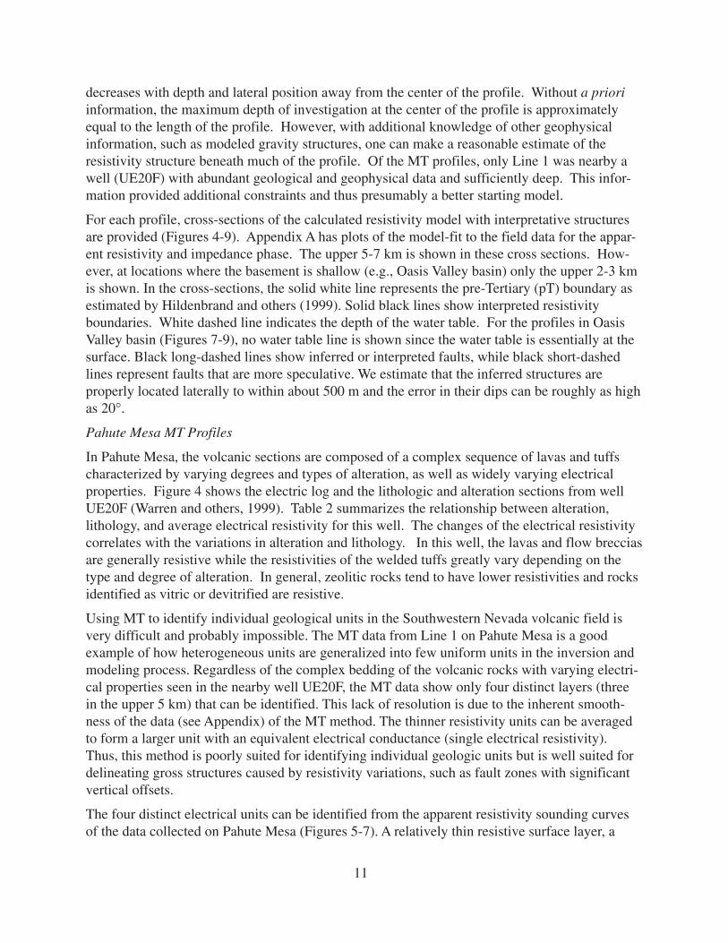
Figure 8: Resistivity cross-section based on the 2D inversion of the MT sounding data alongLine 4. The data were collected across southern end of the Thirsty Canyon lineament (TCL) andthe associated fault zone (TCFZ) near and on the Nellis Air Force Range. The black solid linesrepresent inferred resistivity layer boundaries. The black long dashed lines are inferred faults.The black short dashed lines are more speculative faults. The while solid line is the basementsurface.

0.0 0.5 1.0 1.5 2.0 2.5 3.0 3.5

Distance (km)

2.0

1.5

1.0

0.5

Dep

th (

km)

?

? ?

??

?

pTpT

Resistive Layer

Surface Layer

Resistive pT Basement

WNW ES

18

0 1 2 3

Distance (km)

3

2

1

Dep

th(k

m)

Resistive Layer

Resistive pT Basement

pT

pT

?

S N

Figure 9: Resistivity cross-section based on the 2D inversion of the MT sounding data along

Line 5. The data were collected across east-west trending Colson Pond lineament (CPL) and

magnetic lineament (Mag). The black solid lines represent inferred resistivity layer boundaries.

The black long dashed lines are inferred faults. The black short dashed lines are more specula-

tive faults. The while solid line is the basement surface.

layer (>500 Ω⋅m) appears to be thicker (~2 km) within the Silent Canyon caldera but thins (~500m) outside the caldera. The pT basement dips from west to east into the Silent Canyon caldera.

Line 3 (stations m03-m10) crosses the Buckboard Mesa lineament (BML, Figure 7). The modelshows that the resistive surface layer thickens between m06 and m08. An inferred south-dippingfault beneath station m06 divides the conductive second layer (50-100 Ω⋅m) into a thick (~2 km)zone on the north and a thinner (~800 m) zone on the south. Between station m08 and m09 ahighly conductive zone extends from near the surface down into, and possibly through, theconductive second horizon. The underlying resistive third layer (~700 Ω⋅m) thickens from 2 kmto 4 km as the pT basement surface dips which possibly reflects the thickening of volcanic rockssouthward within the Timber Mountain caldera.

19

Lithology AlterationAverage

Resistivity(Ω⋅m)

Total Thickness(m)

LA -- 2581 305LA GL 1670 101LA GL-DV 403 27LA DV 391 266LA QC 2318 66LA ZE 919 9LA ZC 60 37FB GL-ZE 757 21FB DV 471 338FB AR 223 107BS AR 41 5PL ZA 38 56

BED ZA 140 191BED ZC 61 74NWT -- 398 144NWT AB 51 61NWT QC 63 73NWT ZA 161 833NWT ZC 48 66MWT 693 210MWT DV 390 312MWT QC 70 180RWT ZC 28 159RWT ZE 430 10

Lithology Symbols: LA = lava, FB = flow breccia, BS = basalt, PL = pumiceous lava,BED = bedded tuffs, NWT = non-welded tuffs, MWT = moderately welded tuffs, RWT =reworked tuffs.

Alteration Symbols: GL = vitric, GL-ZE = vitric and minor zeolitic, GL-DV = vitric andminor devitric, DV = devitrified, AR = argillic, AB = albitic, QC = silicic withchalcedony, ZE = zeolitic, ZC = zeolitic with clinophlolite, ZA = zeolitic with analcime.Table 2: Table of alteration, lithology and average electrical resistivity for well UE20F.

Oasis Valley Basin MT Profiles

T he MT soundi ngs col lect ed in Oasi s Val ley basin (F igur es 8- 10) det ect only t wo resi sti vi tyl ayer s above the pT basem ent. A conducti ve surf ace l ayer is pr oduced, i n par t , by t heconduct i ve gr oundwat er ( t ypical l y <5 Ω⋅ m ) and the very shal low wat er t abl e. F or F i gures8-10, t he wat er t abl e li ne is not shown since the wat er level i s at or very near t he surf ace.T he dissol ved sol ids concentr at i on and conduct ivi ty m easur ed fr om water sam pl es in well sat the mouth of T hi r st y Canyon are ~440 m g/ l and ~650 µ S /cm (~1.5 Ω⋅ m ), r especti vel y( Whit e, 1979; T homas, wr i tt en samples i n wel ls at t he m out h of Thir sty Canyon ar e ~440m g/ l and ~650 µ S /cm ( ~1. 5 Ω⋅ m ), respect i vely (Whit e, 1979; T hom as, wri tt en

20

communication, 1998). A stratigraphic cross-section from the Coffer well (Figure 3; Grauch andothers, 1997) shows at least 200 m of alluvium or valley fill. Because the conductive layer in themodels is usually thicker than 200 m, this layer probably includes altered tuffs. An intermediateresistive layer, probably volcanic rocks, lies between the conductive surface and resistive the pTbasement.

The WNW-trending Line 4 (sites n01-n08) in Figure 7, near the possible termination of theTCFZ (Mankinen and others, 1999) shows that basement shallows (~1km). Similar to Lines 1and 2, the TCFZ appears to be characterized by higher conductivities and vertical discontinuities.Between sites n05 and n06, the model shows a surface resistive zone that may be associated witha magnetic low (Mankinen and others, 1999). The moderately resistive second layer (100-500Ω⋅m) undulates (probably due to faulting) and has a thickness of ~400 m (east of station n03).

The north-south profile (Line 5, Figure 8) crosses the Colson Pond lineament (CPL). The modelshows that the surface conductive layer (<10-50 Ω⋅m) is about 300-400 m thick. Betweenstation n12 and n14, this layer thickens (~700 m) possibly due to alteration within a fault zone.This interpreted fault zone may extend from the surface conductive layer down into the base-ment. The unaltered volcanic layer (middle layer) is about 500 m thick to the north and thickenssouthward to ~1.2 km on the southern end of the profile. The resistive (≥3,000 Ω⋅m) pT base-ment dips southward beginning in the region of the interpretative fault zone.

The north-south profile (Line 6, Figure 9) crossing the southern margin of Oasis Valley basin(OVBS, Figure 3) shows a shallow pT basement on the south end of the profile, which rapidlydescends northward into the Oasis Valley basin. The variable thickness of the conductive (10-50Ω⋅m) surface layer is probably related to degrees of alteration. However, below station s18, themodel shows a very conductive block extending into the resistive (300-800 Ω⋅m) second unit.Below the conductive surface layer, the resistive zone may be composed of two electricallydifferent units. The overlying resistive (~800 Ω⋅m) layer extends to a depth of about 2 km andappears to terminate to the south beneath stations s22 and s23. The thickest section of this unit,below site s16 and s15, corresponds with a local magnetic low (Mankinen and others, 1999).This relatively thick upper resistive layer may possibly to due to a dense lava flow. The underly-ing less resistive (~300 Ω⋅m) layer fills the basin north of the inferred fault zone and may becomposed of volcanic tuffs. An alternative model that fits the MT data is a resistive dome (700-1,000 Ω⋅m), possibly a rhyolitic dome, rising from the basement to a depth of about 1.5 km.This resistive dome would correlate with the magnetic low. Additional data are needed to deter-mine which of the two models, a lava flow (2D) or a dome (3D), is preferred.

Discussion

MT data identified three distinct resistivity layers on Pahute Mesa and two layers in the OasisValley basin region within the upper 5 km of the earth. These layers are a surface layer (resistiveon Pahute Mesa and conductive in Oasis Valley), a conductive second layer (only on PahuteMesa), and a deep resistive layer. Based on constraints from gravity studies (Mankinen andothers, 1999; Hildenbrand and others, 1999), the lower resistive layer is divided into an upperresistive volcanic layer and a more resistive pT basement. Prominent lateral variations within the

21

0.0 1.0 2.0 3.0 4.0 5.0

Distance (km)

5.0

4.0

3.0

2.0

1.0

Dep

th(k

m)

pT

pT

Volcanic

Resistive Volcanic

Resistive pT Basement

Resistive Volcanic

?

? ?

?

?

S NFigure 10: Resistivity cross-section based on the 2D inversion of the MT sounding data along

Line 6. The data were collected in the southern end of the Oasis Valley basin (OVBS). The black

solid lines represent inferred resistivity layer boundaries. The black long dashed lines are in-

ferred faults. The black short dashed lines are more speculative faults. The while solid line is the

basement surface.

volcanic rocks above basement are suggested, especially in the surface and conductive layers.Some of the variations may be related to localized surface inhomogeneities and, at depth, toinferred faults juxtaposing rocks of different electrical properties. Units with low resistivitypresumably reflect rocks containing zeolites and clay minerals. Also low resistivities occurwithin fault zones where fractures in the rock expose greater surface area to groundwater, andthus are more susceptible to alteration (probably clays). These observations, in conjunction withavailable gravity and magnetic data, appears to reveal several interesting structures that mayinfluence the groundwater flow from Pahute Mesa to Oasis Valley.

The soundings collected on Pahute Mesa detect a thick conductive layer generally extendingfrom near the water table to a depth of roughly 2 km (Figure 4-6). This conductive layer isprobably the zeolite zonation of the volcanic rocks. On Pahute Mesa, zeolite zonation occurs in

22

the volcanic layers and can have thickness of up to 1 km (Hay, 1966; Hoover, 1968). In severallocations, the upper section of the zonation contains clay minerals followed by a sequence ofzeolite minerals (Hoover, 1968). The existence of this conductive layer makes it possible todetect lateral changes in resistivities at its boundary with the surrounding resistive rocks. Inother words, lateral changes in lithology (such as faulting) are clearly expressed along the upperand lower surfaces of the conductive layer as abrupt changes or undulations in resistivity. Con-versely, within the conductive zone, the rock resistivity becomes more uniform and structures areharder to define. Thus, several of the near-surface inferred faults in our models may actuallyextend deep into the conductive layer.

Thirsty Canyon Fault Zone

The 2-km-wide TCFZ trends SW for at least 35 km from Pahute Mesa to the Oasis Valley basin(Mankinen and others, 1999). Hildenbrand and others (1999) proposed that this fault zoneextends NE of our study area where it is buried beneath alluvial deposits on Gold Flat (Figure 1).They also suggested that this fault zone may continue on trend into the Oasis Valley region orhave a left lateral offset within the basin.

Lines 1, 2, and 4 located over the TCFZ detect abrupt lateral changes in resistivity, possiblyexpressing faults within the zone. Only Line 4 (and possibly Line 2) may have been positionedover the entire TCFZ. Several of the inferred shallow faults (Figures 4, 5, and 7) probablyextend down to basement and may be related to the formation of the Silent Canyon caldera(Lines 1 and 2) and Timber Mountain caldera (Line 4). This inference seems to support theinterpretation of Hildenbrand and others (1999) that the TCFZ expresses a pre-existing basementfault zone that influenced caldera formation. The MT data appear to show that this basementfault zone extends upward to the near surface. Evidently, the vertical stress related to the col-lapse of these calderas was accommodated by existing faults of the TCFZ. The absence of acontinuous surface expression of the TCFZ from the Oasis Valley basin to Pahute Mesa is prob-ably due to younger volcanic units (e.g., those of the Black Mountain caldera) overlying andmasking older faults of the TCFZ.

Resistivities within the TCFZ appear to be lower and more variable than those resulting fromzeolitization, possibly suggesting alteration of the volcanic rock (e.g., forming clay minerals)along the fault surfaces. Extensive faulting creates greater surface areas, increases the suscepti-bility to alteration and thus decreases the rock resistivity. Evidence that fractures are susceptibleto alteration is observed in tunnels and from core samples taken from wells where clayey faultgouge and clay minerals commonly sealed fractures in the tuffs (Thordarson, 1965; Winogradand Thordarson, 1975). However, clay alteration was not commonly found in core samples takenfrom wells on Pahute Mesa (Drellack and others 1997; Prothro, written communication, 1999).Hence, a dense network of open interconnected fractures filled with conductive fluid may be analternative interpretation for the low resistivities within the TCFZ.

The MT data detect only small variations on the basement surface along Line 4. Because thesesmall undulations would produce subtle or no gravity anomalies, Mankinen and others (1999)state that gravity data cannot detect the TCFZ along Line 4. If the observed basement undula-tions are real, the MT data suggest that the TCFZ extends into Oasis Valley basin, at least to Line4, as a series of faults producing small undulations or offsets on the surfaces of the conductivelayer.

23

Oasis Valley Basin

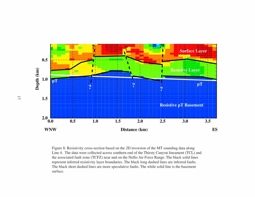
The Oasis Valley basin is a rectangular area on the west side of the exposed part of the SWNVFcaldera complex (C.J. Fridrich, USGS, written communication, 1999). Because of poor exposurein many areas, the boundaries of this basin are defined by geophysical methods. The westernand southern boundaries of Oasis Valley basin are defined by the Hogback and southern struc-tural margin of the Rainier Mesa caldera, respectively. The northwestern and eastern edges ofthe basin are formed by the southern margin of the Black Mountain and the western margin ofthe Transvaal Hills, respectively. Internal and marginal structures, such as the TCFZ, the sourceof the CPL, and OVBS (Figure 1) are apparent on magnetic and gravity maps (Mankinen andothers, 1999). Lines 5 and 6 cross major structures of the Oasis Valley basin (C.J. Fridrich,USGS, written communication, 1999).

The Colson Pond lineament (CPL), named by Fridrich (USGS, written communication, 1999), isan EW-striking feature identified with gravity and magnetic data (Hildenbrand and others, 1999;Mankinen and others, 1999). Fridrich (USGS, written communication, 1999) propose that theCPL is a growth fault formed during the deposition of the Timber Mountain rocks or a strike-slipfault that offsets deep basin sections against outer basin sections. Large changes in stratigraphicthicknesses are probably present across this structure (C.J. Fridrich, USGS, written communica-tion, 1999). The MT data (Figure 8) support a south-dipping fault in the vicinity of the CPL.The thickening of the low resistivity layer associated with the fault zone is probably due toaltered volcanic rock and sediment. The low resistivity values associated with the surface layerare probably due to the saturated and altered alluvium.

The southern structural margin of the Rainier Mesa caldera appears to coincide with the southernboundary of the Oasis Valley basin (Figure 1). This structure may delineate an accommodationfault or zone that transfers strain between different structural domains (C.J. Fridrich, USGS,written communication, 1999). The MT model (Line 6, Figure 9) supports the basin thicknessmodel of Hildenbrand and others (1999) with up to 3-3.5 km of relief on basement in the south-ern part of the basin. However, the MT data can be modeled with a steeper fault (dip ~75°-80°)along the southern margin of the basin. The fault zone probably extends into the overlyingvolcanic rocks to a depth of at least 500 m due to a shallow conductive body lying directly abovethe faulted basement surface (Figure 9). We propose that this conductive source is related toalteration along a highly fractured zone.

Buckboard Mesa Lineament

A ESE-striking magnetic lineament (Grauch and others, 1997) extends from the eastern side ofthe Black Mountain caldera (BM, Figure 1) approximately 30 km eastward along the northernboundary of the Timber Mountain caldera (TMC, Figure 1). The central part of this lineament,called the BML (Mankinen and others, 1999), coincides with the topographic wall of the RainierMesa caldera (Grauch and others, 1997). In the area of Line 3 (Figure 3), Grauch and others(1997) indicated that moderately positively magnetized formations (Ammonia Tanks or TopopahSpring Tuffs) abut against highly negatively magnetized rhyolite of Benham (post Tiva Canyon).

In the vicinity of the BML, a proposed fault offsets the conductive layer (at m08, Figure 6). Thisinferred fault probably is related to the topographic wall of the Rainier Mesa caldera. Thus, theincrease in the thickness of the resistive surface layer along the southern part of the profile may

24

reflect a thick zone of welded tuffs that ponded south of the topographic wall. The intenselyconductive source between site m08 and m09 (Figure 6) is likely a local three-dimensional (3D)body. On the magnetic anomaly map (Mankinen and others, 1999), a 1-km-wide intenseanomaly spatially coincides with the conductive source. Moreover, MT skew data (Schenkel,1998) suggest the presence of a 3D, local source.

Hydrologic Implications

Groundwater flow beneath Pahute Mesa occurs through interconnected fault and joint systems inthe Tertiary volcanic rock units (Blankennagel and Weir, 1973). From hydraulic well tests onPahute Mesa, Blankennagel and Weir (1973) proposed that the rock units easily transmittingwater are rhyolite lavas while the zeolitized tuffs have very low permeabilities (Blankennageland Weir, 1973). Lava, which is a relatively impermeable rock, transmits water readily in PahuteMesa due to the numerous connected fractures that tend to remain open. Welded tuffs also arefound to be good aquifers since they have high fracture permeability and moderate interstitialpermeability if unaltered (Blankennagel and Weir, 1973, Lazczniak and others, 1996). Recordsfrom holes drilled in the welded tuffs and lava flows suggest open and interconnected network offractures because mud circulation was repeatedly lost during drilling. These fractures are usuallyformed in response to tensional forces active during the cooling phase of the flow. Winograd andThordarson (1975) found that fractures make up a small percentage (<2%) of the volume in coresamples but appear to control the transmissibility of rocks. Most of the ash-fall and nonweldedash-flow tuffs in the saturated zone are zeolitized. Water flowing in zeolitized units are alsothrough fractures (Thordarson, 1965). However, fractures in these rock types tend to heal morereadily and are more susceptible to alteration, reducing its transmissivity (Winograd andThordarson, 1975; Blankennagel and Weir, 1973; Lazczniak and others, 1996).

Hildenbrand and others (1999) proposed that basement in the study area consists mainly ofclastic sedimentary rock rather than carbonate rock. Clastic sedimentary rock, particularly thefine-grained quartzite and argillite at Bare Mountain and Bullfrog Hills, is resistant to fracturing.If fractured, they tend to be disconnected. Thus basement probably is a barrier to groundwaterflow.

Synder (1968) and Blankennagel and Weir (1973) pointed out that on Pahute Mesa the rock unitsthat easily transmit water through open interconnected fracture (rhylotic lavas and denselywelded tuffs) are relatively resistive. The rocks with poor transmissivity due primarily tozeolitization and alteration (sealing fractures and pore space) of the ash-fall and nonwelded ash-flow tuffs are electrically conductive. Using these relations, one may infer subsurface structuresthat may influence groundwater flow based on the distribution of the electrical resistivity. Here,we explore the possible effects of the interpreted structures on the groundwater flow from PahuteMesa to the Oasis Valley basin.

Thirsty Canyon Fault Zone

The concept of southwesterly flow of groundwater from Pahute Mesa towards Oasis Valley basinis based on a SW-trending flow barrier (WLD, Figures 1 and 2) proposed by Blankennagel andWeir (1973) from hydraulic gradients taken from contoured water level data. They suggestedthat this barrier juxtaposes low permeable rock on the west against more permeable rock on the

25

east. Water chemistry also supported this concept (Blankennagel and Weir, 1973; Laczniak andothers, 1996; Kilroy and Savard, 1995). This barrier is spatially near if not actually within theTCFZ. Because the TCFZ juxtaposes rocks of different permeabilities, it is likely to act as abarrier to transverse groundwater flow.

Three MT profiles cross the TCFZ, two on Pahute Mesa and one in the Oasis Valley basin nearits terminus. Along each profile the TCFZ appears to be characterized by very low resistivitiesand near-vertical discontinuities assumed to define faults. The low resistivities (<50 Ω-m) mayreflect alteration (possibly clays) along fractured rock. Clay minerals form if the cations releasedby hydrogen exchange are flushed (Hoover, 1968). This requires water flowing through frac-tures at the time the clay minerals were formed. Hence, it is likely that the conductive TCFZ ishighly fractured and acts as or at one time was a conduit for southward flow of groundwater.Thus, the fractures within the TCFZ may act as a barrier or a conduit to groundwater flow,depending on the degree of alteration and its effect on permeability. However, clay alterationwas not common in samples taken from wells at Pahute Mesa (Warren and others, 1999; Prothro,written communication, 1999). From 20 samples in cores from 8 wells on Pahute Mesa,Drellack and others (1997) typically found that the clays formed a thin lining on the fracturewalls. Based on the uncommon occurrence of clays found in samples from well on Pahute Mesa,the electrically conductive TCFZ may be due to a higher density of open, interconnected frac-tures filled with conductive groundwater. This implies that the TCFZ would act as a conduit forsouthward flow of groundwater from Pahute Mesa to Oasis Valley. A drill hole within the TCFZwould resolve which interpretation is preferred.

Line 1 (Figure 4) appears to extend over the eastern part of the TCFZ which presumably contin-ues west beyond the profile. Although the western margin of the TCFZ is represented in thecross-section of Line 2, its eastern margin may lie at or beyond the end of the line. South in theOasis Valley basin, Line 4 seems to show that the TCFZ is roughly 2.5 km wide. From thisprofile, the proposed groundwater flow related to the TCFZ may extend SW to, at least, latitude37°05’. The combined effect of shallowing of the impermeable basement and channeling ofwater along the TCFZ toward Oasis Valley basin probably results in a shallow water table and insprings where the TCFZ meets the fault zone associated with the CPL. Thus, the MT data appearto support the conclusion of Hildenbrand and others (1999) that the TCFZ acts a barrier to deepflow and may channel groundwater to the Oasis Valley basin. Recent water chemistry analysisof isotopes and major ion concentration from wells on Pahute Mesa and in Oasis Valley (Kilroyand Savard, 1996; Thomas, 1998, written communication) also supports this conclusion due to adistinct correlation of the groundwater chemistry from Pahute Mesa and that in the Oasis Valleybasin.

Buckboard Mesa Lineament

Line 3 (Figure 6) crosses the BML and presumably a shallow topographic wall related to TimberMountain caldera. The MT data may delineate a south-dipping fault forming a thick resistivesurface layer (south of the fault). Because this resistive layer is likely associated with denselywelded tuffs related to this caldera, the transmissivity of the rocks in the upper 2 km will prob-ably increase from north to south across the fault zone since aquifers are generally found inwelded tuff layers.

26

Oasis Valley Basin

The NS profiles (Lines 5-6; Figures 8-9) show a resistive, probably unaltered volcanic secondlayer (300-700 Ω⋅m) underlying a conductive layer. The inferred fault zone at CPL (Figure 8)and the impermeable basement appear to pinch the resistive volcanic layer in the vicinity of thefault zone, which may affect groundwater flow particularly if a high degree of alteration sealedthe fractures. The conductive nature of the surface layer in the fault zone indicates water move-ment along this inferred fault zone, possibly towards Colson Pond. On the southern end of OasisValley basin (Line 6; Figure 9), a steep north-dipping fault zone offsets basement and youngervolcanic rock at shallow depths (~500 m). The large offset of basement along the southernmargin of the Oasis Valley basin probably reduces southward groundwater flow as basement isassumed to be relatively impermeable. Altered volcanic and sedimentary rocks above the faultzone may act as a barrier diverting groundwater to the SW toward Beatty. If the EW barrier isnot present, groundwater may flow south into Crater Flat.

Conclusion

MT data collected in the Pahute Mesa-Oasis Valley basin region define several structures possi-bly influencing groundwater flow. Using observed relations of the electrical and hydrologicalproperties of the volcanic rocks, structures that control groundwater flow, such as faults, mayhave been tentatively identified. The NE-trending TCFZ, being electrically conductive, mayrepresent a groundwater flow conduit channeling water from Pahute Mesa southwestward intothe Oasis Valley basin. In the southern end of the Oasis Valley basin, a fault zone that may havealtered the surface layer and underlying resistive volcanic layer may also be a possible barrier togroundwater flow. Future research topics should include determining the flow path from theOasis Valley basin (e.g., SW towards Beatty or south into Crater Flat).

Acknowledgements

We thank Jerry Magner and Doug Trudeau (USGS, Las Vegas) for arranging the logistics on theNTS and Nellis Air Force Range and for facilitating our work there. We are extremely gratefulto Don Schaefer, Jay Sampson, Jackie Williams, Bob Bisdorf, Roy Kipfinger, Kip Allander, JeffDavidson, and Ted Asch (EMI) who assisted in the collection of the field data on Pahute Mesaand in Oasis Valley. We also wish to thank EMI for their technical support and access to theirfacilities during the acquisition and processing of the data. We are indebted to Mike Hoversten(LBL) for his time and knowledge of MT data analysis and his software made available for use.Discussions with Mike Hoversten and Frank Morrison (U.C. Berkeley) were very useful in theanalysis and interpretation of the MT data. Conversations with Ted McKee, Chris Fridrich,Randy Laczniak, and Jim Thomas greatly improve our models and conclusions, although theiraccuracy are solely the responsibility of the authors. We also acknowledge the useful perspec-tives and thoughtful comments on this manuscript by: Lance Protho, Sig Drellack, MargaretTownsend, Ward Hawkins, Bruce Hurley, Gayle Palowski and Paul Kasameyer. We also want tothank Paul Stone for his editorial comments. This work is part of an interagency effort betweenthe USGS and the U.S. Department of Energy and was funded through the Interagency Agree-ment DE-AI08-96NV11967.

27

References

Blankennagel, R.K. and Weir, J.E., Jr., 1973, Geohydrology of the eastern part of Pahute Mesa,Nevada test Site, Nye County, Nevada: U.S.G.S. Professional Paper 712-B, 35p.

Cagniard, L., 1953, Basic theory of the magneto-telluric method of geophysical exploration:Geophysics, 18, p. 605-635.

Drellack, Jr., S.L., Prothro, L.B., Roberson, K.E., Schier, B.A., and Price, E.H., 1997, Analysis offractures in volcanic cores from Pahute Mesa, Nevada Test Site: DOE/NV/11718-160,Las Vegas, NV.

Ekren, E.B., 1968, Geological setting of Nevada Test Site and Nellis Air Force Range, in Eckel,E.B., ed., Nevada Test Site: Geological Society of America, Memoir 110, p. 11-20.

Furgerson, R.B., 1982, Remote-reference magnetotelluric survey, Nevada Test Site and vicinity,Nevada and California, with an introduction by D.B. Hoover: U.S.G.S. Open-File Report82-465, 156p.

Gamble, T.D., Goubau, W.M., and Clarke, J., 1979, Magnetotellurics with remote reference:Geophysics, 44, p. 53-68.

Grauch V.J.S., Sawyer, D.A., Fridrich C.J., and Hudson M.R., 1997, Geophysical interpretationswest of and within the northwestern part of the Nevada test site: U.S.G.S. Open-FileReport 97-476, 45p.

Hay, R.L., 1966, Zeolites and zeolitic reactions in sedimentary rock: Geological Society ofAmerica, Special Papers number 85, 130p.

Hildenbrand, T.G., Langenheim, V.E., Mankenin, E.A., and McKee, E.H., 1999, Inversion ofgravity data to define the pre-Tertiary surface of the Pahute Mesa-Oasis Valley region,Nye County, Nevada: U.S.G.S. Open File Report 99-49, 26p.

Hoover, D.L., 1968, Genesis of Zeolites, Nevada Test Site, in Eckel, E.B., ed., Nevada Test Site:Geological Society of America, Memoir 110, p. 275-284.

Hoover, D.B., Hanna, W.F., Anderson, L.A., Flanigan, V.J., and Pankratz, L.W., 1982a, Geo-physical studies of the Syncline ridge area, Nevada Test Site, Nye County, Nevada:U.S.G.S. Open File Report 82-145, 55p.

Hoover, D.B., Chornack, M.P., Nervick, K.H., and Broker, M.N., 1982b, Electrical Studies at theproposed Wahmonie and Calico Hills nuclear waste sites, Nevada Test Sites, Nye Co.,Nevada: U.S.G.S. Open-File Report 82-466, 45p.

Keller, G.V., 1987, Rock and mineral properties, in Electromagnetic Methods in Applied Geo-physics-Theory: Nabighian, M.N., ed., Society of Exploration Geophysicists, Tulsa, Ok,v 1, p. 13-51.

Keller, G.V. and Frischknecht, F.C., 1966, Electrical methods in geophysical prospecting:Pergammon Press, New York, 517p.

Kilroy, K.C. and Savard, C.S., 1995, Geohydrology of Pahute Mesa-3 test well, Nye County,Nevada: U.S.G.S. Water Resources Investigations Report 95-4239, 37p.

Klein, D.P., 1995, Chapter 4: Regional magnetotelluric investigations, in Oliver, H.W., Ponce,D.A., and Hunter, W.C., eds., Major results of geophysical investigations at Yucca Moun-tain and vicinity, southern Nevada: Open-File Report 95-74, p. 73-97.

Laczniak, R.J., Cole, J.C., Sawyer, D.A., and, Trudeau, D.A., 1996, Summary of hydrogeologiccontrols on ground-water flow at the Nevada Test Site, Nye County, Nevada: U.S.G.S.Water-Resources Investigations Report 96-4109, 59p.

28

Mankinen, E.A., Hildenbrand, T.G., Roberts, C.W., and Davidson, J.G., 1998, Principle facts fornew gravity stations in the Pahute Mesa and Oasis Valley areas, Nye County, Nevada:U.S.G.S. Open-File Report 98-498, 14p.

Mankinen, E.A., Hildenbrand, T.G., Dixon, G.L., McKee, E.H., Fridrich C.J., and Laczniak, R.J.,1999, Gravity and magnetic study of the Pahute Mesa and Oasis Valley region, NyeCounty, Nevada, U.S.G.S. Open File Report 99-303, 57p.

Maldonado, F., Muller, D.C., and Morrison, J,N., 1979, Preliminary geological and geophysicaldata of the UE25a-3 exploratory drill hole, Nevada Test Site, Nevada: USGS-1543-6,47p.

Noble, D.C., Weiss, S.I., and McKee, E.H., 1991, Magmatic and hydrothermal activity, calderageology, and regional extension in the western part of the southwestern Nevada volcanicfield, in Raines, G.L., Lisle, R.E., Schaefer, R.W., and Wilkinson, W.H., eds., Geologyand ore deposits of the Great Basin, Symposium Proceedings: Reno, Geological Societyof Nevada, p. 913-934.

Olhoeft, G.R., 1981, Electrical properties of granite with implications for the lower crust: JournalGeophysical Research, 86, p. 931-936.

Olhoeft, G.R., 1980, Electrical properties of rocks, in Physical Properties of Rocks and Minerals:Touloukian, Y.S., Judd, W.R., and Roy, R.F., eds., McGraw-Hill, New York, p. 257-330.

Palacky, G.J., 1987, Resistivity characteristics of geologic targets, in Electromagnetic Methods inApplied Geophysics-Theory: Nabighian, M.N., ed., Society of Exploration Geophysi-cists, Tulsa, Ok, v 1, p. 53-129.

Plouff, Donald, 1966, Magnetotelluric soundings in the southwestern United States: Geophysics,v. 31, p.1145-1152.

Sawyer, D.A., Fleck, R.J., Lanphere, M.A., Warren, R.G., Broxton, D.E., and Hudson, M.R.,1994, Episodic volcanism in the southwest Nevada volcanic field: Revised stratigraphicframework, Ar40/Ar39 geochronology, and implications for magnetism and extension:Geological Society of America Bulletin, 106, no. 10, p. 1304-1318.

Schenkel, C.J., 1998, Magnetotelluric data in the Pahute Mesa and Oasis Valley areas, NyeCounty, Nevada: U.S.G.S. Open-File Report 98-504, 70p.

Snyder, R.P., 1968, Electric and caliper logs as lithologic indicators in volcanic rocks, NevadaTest Site: in Eckel, E.B., ed., Nevada Test Site: Geological Society of America, Memoir110, p. 117-124.

Thordarson, W., 1965, Perched ground water in zeolitized-bedded tuff, Rainier Mesa and vicin-ity, Nevada Test Site, Nevada: U.S.G.S. Trace Elements Investigations Report TEI-862,90p.

Tikhonov, A.N., 1950, On determining electrical characteristics of the deep layers of the earth’scrust: Doklady, 73, p. 295-297.

Torres-Verdin, C., 1991, Continuous profiling of magnetotelluric fields: Ph.D. thesis, Universityof California, Berkeley.

Torres-Verdin, C. and Bostick, F.X., Jr., 1992, Principles of spatial surface electric field filteringin magnetotellurics; Electromagnetic array profiling (EMAP): Geophysics, 57, p. 603-622.

U.S. Department of Energy, 1994, United States nuclear tests; July, 1945 through September,1992; U.S. Department of Energy, Nevada Operation Office, DOE/NV-209 (rev 14),105p.

29

Vozoff, K., 1972, The magnetotelluric method in the exploration of sedimentary basins: Geo-physics, 37, p. 98-141.

Vozoff, K. (editor), 1986, Magnetotelluric Methods: Geophysics reprint series no. 5, Society ofExploration Geophysicists, Tulsa, OK, 763p.

Vozoff, K., 1991, The magnetotelluric method: in Nabighian, M.N., Ed., Electromagnetic Meth-ods in Applied Geophysics, v. 2, Application, Part B, Society of Exploration Geophysi-cists, Tulsa, p. 641-711.

Wahl, R.R., Sawyer, D.A., Minor, S.A., Carr, M.D., Cole, J.C., Swadley, W.C., Laczniak, R.J.,Warren, R.G., Green, K.S., and Engle, C.M., 1997, Digital geologic map of the NevadaTest Site area, Nevada: U.S.G.S. Open-File Report 97-140, scale 1:120,000.

Warren, R.G., Sawyer, D.A, Byers, Jr., F.M., and Cole, G.L., 1999, A petrographic/geochemicaldatabase and structural framework for the Southwestern Nevada Volcanic Field: availablefrom the National Geophysical Data Center at http://queeg.ngdc.noaa.gov/seg/geochem/swnvf.

Winograd, I.J. and Thordarson, W., 1975, Hydrogeologic and hydrochemical framework, South-Central Great Basin, Nevada-California, with special reference to the Nevada Test Site:U.S.G.S. Professional Paper 712-C, 126p.

White, A.F., 1979, Geochemistry of ground water associated with tuffaceous rocks, Oasis Valley,Nevada: U.S.G.S. Professional Paper 712-E, 25p.

White, A.F., Claassen, H.C., and Benson, L.V., 1980, The effects of dissolution of volcanic glasson the water chemistry in a tuffaceous aquifer, Rainier Mesa, Nevada: U.S.G.S. WaterSupply Paper 1535-Q, 34p.

30

Appendix A

Concept of Magnetotellurics

The fundamentals of magnetotellurics (MT) as an exploration method were developed byTikhonov (1950) and Cagniard (1953), in context of one-dimensional (1D) resistivity models.Papers by Vozoff (1972, 1986, and 1991) and Furgerson (1982) give overviews of this techniquefor 2D and 3D situations. MT is an electromagnetic sounding technique that uses measurementsof the natural surface electric (E) and magnetic (H) fields to infer the subsurface electrical resis-tivity distribution.

The natural sources of MT fields come from lightning discharges and magnetospheric currentsystems set up by solar activity. These sources create a spectrum of EM fields in the frequencyband 10-4 to 104 Hz, which provide information to delineate structures at depth from a few tens ofmeters to the upper mantle at a few tens of kilometers. MT data at various frequencies provide ameans to distinguish spatial variations in resistivity vertically and laterally. The EM field pen-etration, which decays exponentially, is related to the frequency and resistivity of the medium.Higher frequencies map the near-surface resistivity distribution. Lower frequencies whichpenetrate farther provide information on deeper structures. However, lateral inhomogeneitieswill also influence these measured fields at equivalent distances from the measurement point.

Time-varying H-fields, which behave almost like plane waves at the surface of the earth, areproduced from the natural sources. Because of the high refractory index at the air-earth inter-face, most of the energy is reflected but a small amount is propagated vertically downward intothe earth. Through Faraday’s Law the H-fields produce an electromotive force (emf) in theconducting earth that causes electric currents to flow within the earth. Spectral estimation tech-niques are used to obtain a frequency and space dependent, 2x2 surface impedance matrix, Z,relating linearly orthogonal E-field and H-field values measured at the same point on the surfaceof the earth. By sampling Z from a number of locations within the survey area, one can infer thedistribution of subsurface electrical resistivity.

For a 1D layered half-space, the off-diagonal elements of the surface impedance tensor (Zxy andZxy) are the same. However, if the ground is inhomogeneous, the surface impedance compo-nents are different. If the surface impedance tensor is rotated so that the diagonal elements (Zxxand Zyy) are minimized (close to zero), the off-diagonal elements, Zxy and Zyx, are called theprinciple impedances and the angle of rotation is the impedance strike direction. The impedancestrike direction and its orthogonal complement make up the principle axes; the impedance strikehas an inherent 90° shift ambiguity that is usually resolved from the Tipper data (see Vozoff,1991), or from the frequency relationships of the various impedance elements.

If one assumes that a survey profile direction (x-axis) is collected orthogonal to the geoelectricstrike direction (y-axis), the two modes (orthogonal components) of the surface impedance arealong the principle axes. For a 2D structure, the Zxx and Zyy components are zero. The surfaceimpedance is composed of two modes. One mode is where the electric field is parallel with theelectrical strike direction and is called the transverse electric (TE) mode. The other, the trans-verse magnetic TM mode, is where the electric field is along the profile direction (orthogonal tothe strike). The TM mode is sensitive to lateral discontinuities since the electric field will changeacross a lateral boundary. In general, the two impedance components are presented as sounding

31

curves showing the apparent resistivities modes, ρTM

and ρTE

, and impedance phases (θTM

and θTE

) for the two modes as a function of frequency as sounding curves. If the data express a layeredmedium, the apparent resistivity (ρ

TM and ρ

TE) are the same. However, if the two curves diverge,

a 2D or 3D structure is likely present. The skew (see Vozoff, 1991), which is a function of Zxxand Zyy, can be used to determine if the structure is 2D or 3D. In theory, the skew should be zero(near zero) for a 2D or 1D medium.

Factors Influencing the Electrical Properties

A given geologic unit can have changes in resistivity due to variations in the pore fluid resistivityand the fluid volume, both of which are controlled by various geologic processes. Ionic exchangebetween minerals and pore fluids at the pore interface is an important factor in the resistivity ofthe rock (Keller and Frischknecht, 1966; Olhoeft, 1980 and 1981, Keller 1987, and Palacky,1987). Increased ionic content and dissolved solid concentrations in the pore fluid will reducethe resistivity of saturated rocks. Pore space in the rock is affected by two main factors. Thefirst factor is the emplacement process which affects porosity (thus the amount of water present);deposits that have greater porosity tend to have lower resistivity. The second factor is related togeologic processes such as alteration or mineralization. These processes can have a significanteffect on the resistivity of the rock by filling the pore spaces and changing the ionic content ofthe pore fluid.

The dominant ionic constituents of the groundwater in the vicinity of the TCL (beneath westernpart of Pahute Mesa) are sodium (cation) and bicarbonates (anion) (Blankennagel and Weir,1973). The relatively high concentration of these ions is probably due to the volcanic tuffs thatcomprise the principal volcanic rock types in the saturation zone of this area. In addition to theabundant amounts of bicarbonates, sulfates and chloride anions exist in relatively large amounts.The concentration of chemical constituents in the groundwater in this area is relatively uniformand greater than that in the eastern part of Pahute Mesa. The dissolved solids in the water rangesfrom 206 to 336 milligrams/liter (mg/l) and average 280 mg/l. The high amounts of ions anddissolved solids produces relatively conductive groundwater where the specific conductance ofthe groundwater ranges from ~300 to >500 µS/cm (0.3-0.5 S/m or 2.0-3.3 Ω⋅m).

The rhyolitic volcanic rocks typical in the study area are lava flows, bedded ash-fall tuffs, andash-flow tuffs with various degrees of welding. In a water-saturated environment, the volcanicrocks exhibiting greater porosity tend to be less electrically resistive. In general, bedded ash-falltuffs generally exhibit porosities (≥40%) greater than flow rocks (Winograd and Thordarson,1975); consequently ash-fall tuffs tend to have the lowest resistivity. Additionally, these rocks arethe most susceptible to alteration and secondary mineralization. In the ash-flow rocks, as weldingincreases, pore space decreases resulting in higher resistivities. Winograd and Thordarson (1975)found that nonwelded tuffs have porosities of up to 40% while the porosity of densely weldedtuffs range from 4% to 13%. Thus, resistivity will increase as the welding in ash-flow tuffsincreases. Lava flows with very little porosity (2-15%) (Blankennagel and Weir, 1973) generallyhave the highest resistivities. The fractures in the lavas and densely welded tuffs will increase theeffective permeability of the rock.

At the NTS, vitric rock reacts with the groundwater to produce zeolites, cristobalite, quartz, K-feldspar, and clay minerals (Hoover, 1968). The alteration of the volcanic rocks on Pahute Mesa

32

occurs in the presence of fluid (Hoover, 1968). Vitric rocks can form clay minerals only if theyare unsaturated and drained rapidly; while zeolite minerals require a saturated environment toform (Hoover, 1968). Zeolites precipitate from solution typically into the pore spaces or cavitiesof the tuffs (Hay, 1966). On Pahute Mesa, a common alteration mineral associated with zeolitesis montmorillonite (clay) (Thordarson, 1965; Hoover, 1968, White and others, 1980). Zeoliteand clay minerals decrease the rock resistivity due to the increase in surface conduction arisingfrom the ionic exchange between the fluid and minerals at the pore-wall interface. Mineralsexhibiting cation exchange capacity (the quantity of exchangeable cations attached to a mineral)tend to have lower resistivities. Clay minerals are commonly known to have high exchangecapacities. Zeolite minerals have cation exchange capacity greater than some clay minerals(Keller and Frischknecht, 1966). In fact, all fine-grained minerals including quartz have anappreciable cation exchange capacity and the exchange capacity is larger for finer grained par-ticles (Keller and Frischknecht, 1966). Since all rocks possess some exchange capacity, theresistivity of the fluid in a pore space will always be decreased by ions supplied by desorption(Keller and Frischknecht, 1966). Thus, as the amount of zeolites and clay minerals increase,resistivity decreases in volcanic rock.

From electric well logs, Snyder (1968) and Blankennagel and Weir (1973) showed good relationsbetween volcanic rock types on Pahute Mesa and representative electrical resistivities.Resistivities of the rhyolitic lavas range from over 225 Ω⋅m to more than 1,000 Ω⋅m. Thedensely welded tuffs have resistivities in the same range as those of the rhyolitic lavas. Mostresistivities of moderately welded tuffs are between 100 Ω-m to 225 Ω-m. Resistivities of rela-tively impermeable zeolitized tuffs are generally <100 Ω⋅m. The resistivities of vitric ash-falltuffs, nonwelded to slightly welded ash-flow tuffs, and tuffaceous sediments are similar to thoseof zeolitized units. The lowest resistivities occurred in intervals altered by clay minerals.

Data

The model fit to the field data for Lines 1 to 6 are shown in Figures A-1 to A-6, respectively. Inthe sounding curves (apparent resistivity and impedance phase), the field data for the TM and TEmodes are represented by black lines with squares and circles, respectively. Dark gray (TM) andlight gray (TE) lines show the calculated responses of the models for each MT site (plot title).

Figure A-1 shows that the TM mode of the model closely simulate the field data. Several othermodels based solely on the TM data result in the same general structure. The TE mode data havea poorer fit, especially near the area of the vertical conductive block (p22-p23). This may indi-cate that the conductive block may be more conductive and/or extensive than shown on theresistivity cross-section.

The model response matched the field data of Line 2 for the TM mode (Figure A-2). The TEmode data have a poorer fit, especially near the area of the BML (b02-b04). Since the data arerotated to maximize the response of the TCFZ, the source of the BML may produce a 3D effecton the data. At the sites removed from the BML the simulations of the TE mode match the fielddata well. The misfit of the data and simulations in the phase at the low frequencies indicate thatthe model of the deep conductor is too resistive or too deep. However, this misfit does not affectthe upper section of the model.

The results for Line 3 show that the apparent resistivity and impedance phase for the TM and TE

33

modes are matched well (Figure A-3). The responses from the model were able to closely matchthe field data particularly with the TM mode. Again, the TE mode data have a slightly poorer fitespecially at the low frequencies at site m08 indicating a small local near-surface inhomogeneity.

The simulated and field data are plotted in Figure A-4 for Line 4. The simulated TM apparentresistivity fit the field data well. The TE counterparts match the field data except for the lowfrequencies of n01 and n02. The simulated phase does not match the field result well.

Figure A-5 shows the model fit the field data well for the TM mode (both apparent resistivity andimpedance phase). For the TE mode only the apparent resistivity fit the data while the imped-ance phase has a poor match, especially at n14 and n13. The TE data are very noisy as seen bythe large error bars.

Again, the TM mode of the model and field data fit well (Figure A-6). For the TE mode, theapparent resistivity of the model simulated the field data while the impedance phase has a poorerfit. The TE data are very noisy as seen by the large error bars.

34

Figure A-1: Model fit (boxes) and field data (lines) of the apparent resistivity (left) and imped-ance phase (right) for Line 1. TM and TE modes are black and gray, respectively.

DataTMTE

Model

1E-2 1E-1 1E 0 1E 1 1E 2

Frequency(Hz)

PM2_ALL_RM_200--p15

1E 1

1E 2

1E 3

App

aren

t_R

esis

tivity

(ohm

-m)

1E-2 1E-1 1E 0 1E 1 1E 2

Frequency(Hz)

PM2_ALL_RM_200--p16

1E 1

1E 2

1E 3

App

aren

t_R

esis

tivity

(ohm

-m)

1E-2 1E-1 1E 0 1E 1 1E 2

Frequency(Hz)

PM2_ALL_RM_200--p17

1E 1

1E 2

1E 3

App

aren

t_R

esis

tivity

(ohm

-m)

1E-2 1E-1 1E 0 1E 1 1E 2

Frequency(Hz)

PM2_ALL_RM_200--p18

1E 1

1E 2

1E 3

App

aren

t_R

esis

tivity

(ohm

-m)

1E-2 1E-1 1E 0 1E 1 1E 2

Frequency(Hz)

PM2_ALL_RM_200--p19

1E 1

1E 2

1E 3

App

aren

t_R

esis

tivity

(ohm

-m)

1E-2 1E-1 1E 0 1E 1 1E 2

Frequency(Hz)

PM2_ALL_RM_200--p20

1E 1

1E 2

1E 3

App

aren

t_R

esis

tivity

(ohm

-m)

1E-2 1E-1 1E 0 1E 1 1E 2

Frequency(Hz)

PM2_ALL_RM_200--p21

1E 1

1E 2

1E 3

App

aren

t_R

esis

tivity

(ohm

-m)

1E-2 1E-1 1E 0 1E 1 1E 2

Frequency(Hz)

PM2_ALL_RM_200--p22

1E 1

1E 2

1E 3

App

aren

t_R

esis

tivity

(ohm

-m)

1E-2 1E-1 1E 0 1E 1 1E 2

Frequency(Hz)

PM2_ALL_RM_200--p23

1E 1

1E 2

1E 3

App

aren

t_R

esis

tivity

(ohm

-m)

1E-2 1E-1 1E 0 1E 1 1E 2

Frequency(Hz)

PM2_ALL_RM_200--p24

1E 1

1E 2

1E 3

App

aren

t_R

esis

tivity

(ohm

-m)

1E-2 1E-1 1E 0 1E 1 1E 2

Frequency(Hz)

PM2_ALL_RM_200--p25

1E 1

1E 2

1E 3

App

aren

t_R

esis

tivity

(ohm

-m)

1E-2 1E-1 1E 0 1E 1 1E 2

Frequency(Hz)

PM2_ALL_RM_200--p26

1E 1

1E 2

1E 3

App

aren

t_R

esis

tivity

(ohm

-m)

1E-2 1E-1 1E 0 1E 1 1E 2

Frequency(Hz)

PM2_ALL_RM_200--p27

1E 1

1E 2

1E 3

App

aren

t_R

esis

tivity

(ohm

-m)

1E-2 1E-1 1E 0 1E 1 1E 2

Frequency(Hz)

PM2_ALL_RM_200--p28

1E 1

1E 2

1E 3

App

aren

t_R

esis

tivity

(ohm

-m)

1E-2 1E-1 1E 0 1E 1 1E 2

Frequency(Hz)

PM2_ALL_RM_200--p29

1E 1

1E 2

1E 3

App

aren

t_R

esis

tivity

(ohm

-m)

1E-2 1E-1 1E 0 1E 1 1E 2

Frequency(Hz)

PM2_ALL_RM_200--p30

1E 1

1E 2

1E 3

App

aren

t_R

esis

tivity

(ohm

-m)

1E-2 1E-1 1E 0 1E 1 1E 2

Frequency(Hz)

PM2_ALL_RM_200--p31

1E 1

1E 2

1E 3

App

aren

t_R

esis

tivity

(ohm

-m)

1E-2 1E-1 1E 0 1E 1 1E 2

Frequency(Hz)

PM2_ALL_RM_200--p32

1E 1

1E 2

1E 3

App

aren

t_R

esis

tivity

(ohm

-m)

1E-2 1E-1 1E 0 1E 1 1E 2

Frequency(Hz)

PM2_ALL_RM_200--p33

1E 1

1E 2

1E 3

App

aren

t_R

esis

tivity

(ohm

-m)

1E-2 1E-1 1E 0 1E 1 1E 2

Frequency(Hz)

PM2_ALL_RM_200--p34

1E 1

1E 2

1E 3

App

aren

t_R

esis

tivity

(ohm

-m)

1E-2 1E-1 1E 0 1E 1 1E 2

Frequency(Hz)

PM2_ALL_RM_200--p35

1E 1

1E 2

1E 3

App

aren

t_R

esis

tivity

(ohm

-m)

1E-2 1E-1 1E 0 1E 1 1E 2

Frequency(Hz)

PM2_ALL_RM_200--p15

-180

-120

-60

0

60

120

180

Impe

danc

e_Ph

ase(

degr

ees)

1E-2 1E-1 1E 0 1E 1 1E 2

Frequency(Hz)

PM2_ALL_RM_200--p16

-180

-120

-60

0

60

120

180

Impe

danc

e_Ph

ase(

degr

ees)

1E-2 1E-1 1E 0 1E 1 1E 2

Frequency(Hz)

PM2_ALL_RM_200--p17

-180

-120

-60

0

60

120

180

Impe

danc

e_Ph

ase(

degr

ees)

1E-2 1E-1 1E 0 1E 1 1E 2

Frequency(Hz)

PM2_ALL_RM_200--p18

-180

-120

-60

0

60

120

180

Impe

danc

e_Ph

ase(

degr

ees)

1E-2 1E-1 1E 0 1E 1 1E 2

Frequency(Hz)

PM2_ALL_RM_200--p19

-180

-120

-60

0

60

120

180

Impe

danc

e_Ph

ase(

degr

ees)

1E-2 1E-1 1E 0 1E 1 1E 2

Frequency(Hz)

PM2_ALL_RM_200--p20

-180

-120

-60

0

60

120

180

Impe

danc

e_Ph

ase(

degr

ees)

1E-2 1E-1 1E 0 1E 1 1E 2

Frequency(Hz)

PM2_ALL_RM_200--p21

-180

-120

-60

0

60

120

180

Impe

danc

e_Ph

ase(

degr

ees)

1E-2 1E-1 1E 0 1E 1 1E 2

Frequency(Hz)

PM2_ALL_RM_200--p22

-180

-120

-60

0

60

120

180

Impe

danc

e_Ph

ase(

degr

ees)

1E-2 1E-1 1E 0 1E 1 1E 2

Frequency(Hz)

PM2_ALL_RM_200--p23

-180

-120

-60

0

60

120

180

Impe

danc

e_Ph

ase(

degr

ees)

1E-2 1E-1 1E 0 1E 1 1E 2

Frequency(Hz)

PM2_ALL_RM_200--p24

-180

-120

-60

0

60

120

180

Impe

danc

e_Ph

ase(

degr

ees)

1E-2 1E-1 1E 0 1E 1 1E 2

Frequency(Hz)

PM2_ALL_RM_200--p25

-180

-120

-60

0

60

120

180

Impe

danc

e_Ph

ase(

degr

ees)

1E-2 1E-1 1E 0 1E 1 1E 2

Frequency(Hz)

PM2_ALL_RM_200--p26

-180

-120

-60

0

60

120

180

Impe

danc

e_Ph

ase(

degr

ees)

1E-2 1E-1 1E 0 1E 1 1E 2

Frequency(Hz)

PM2_ALL_RM_200--p27

-180

-120

-60

0

60

120

180

Impe

danc

e_Ph

ase(

degr

ees)

1E-2 1E-1 1E 0 1E 1 1E 2

Frequency(Hz)

PM2_ALL_RM_200--p28

-180

-120

-60

0

60

120

180

Impe

danc

e_Ph

ase(

degr

ees)

1E-2 1E-1 1E 0 1E 1 1E 2

Frequency(Hz)

PM2_ALL_RM_200--p29

-180

-120

-60

0

60

120

180

Impe

danc

e_Ph

ase(

degr

ees)

1E-2 1E-1 1E 0 1E 1 1E 2

Frequency(Hz)

PM2_ALL_RM_200--p30

-180

-120

-60

0

60

120

180

Impe

danc

e_Ph

ase(

degr

ees)

1E-2 1E-1 1E 0 1E 1 1E 2

Frequency(Hz)

PM2_ALL_RM_200--p31

-180

-120

-60

0

60

120

180

Impe

danc

e_Ph

ase(

degr

ees)

1E-2 1E-1 1E 0 1E 1 1E 2

Frequency(Hz)

PM2_ALL_RM_200--p32

-180

-120

-60

0

60

120

180

Impe

danc

e_Ph

ase(

degr

ees)

1E-2 1E-1 1E 0 1E 1 1E 2

Frequency(Hz)

PM2_ALL_RM_200--p33

-180

-120

-60

0

60

120

180

Impe

danc

e_Ph

ase(

degr

ees)

1E-2 1E-1 1E 0 1E 1 1E 2

Frequency(Hz)

PM2_ALL_RM_200--p34

-180

-120

-60

0

60

120

180

Impe

danc

e_Ph

ase(

degr

ees)

1E-2 1E-1 1E 0 1E 1 1E 2

Frequency(Hz)

PM2_ALL_RM_200--p35

-180

-120

-60

0

60

120

180

Impe

danc

e_Ph

ase(

degr

ees)

Impedance PhaseApparent Resistivity

35

Figure A-2: Model fit (boxes) and field data (lines) of the apparent resistivity (top) and imped-ance phase (bottom) for Line 2.TM and TE modes are black and gray, respectively.

1E-2 1E-1 1E 0 1E 1 1E 2

Frequency(Hz)

BJ_R110_RM_ALL_30--b02

1E 0

1E 1

1E 2

1E 3

App

aren

t_R

esis

tivity

(ohm

-m)

1E-2 1E-1 1E 0 1E 1 1E 2

Frequency(Hz)

BJ_R110_RM_ALL_30--b03

1E 0

1E 1

1E 2

1E 3

App

aren

t_R

esis

tivity

(ohm

-m)

1E-2 1E-1 1E 0 1E 1 1E 2

Frequency(Hz)

BJ_R110_RM_ALL_30--b04

1E 0

1E 1

1E 2

1E 3

App

aren

t_R

esis

tivity

(ohm

-m)

1E-2 1E-1 1E 0 1E 1 1E 2

Frequency(Hz)

BJ_R110_RM_ALL_30--b05

1E 0

1E 1

1E 2

1E 3

App

aren

t_R

esis

tivity

(ohm

-m)

1E-2 1E-1 1E 0 1E 1 1E 2

Frequency(Hz)

BJ_R110_RM_ALL_30--b06

1E 0

1E 1

1E 2

1E 3

App

aren

t_R

esis

tivity

(ohm

-m)

1E-2 1E-1 1E 0 1E 1 1E 2

Frequency(Hz)

BJ_R110_RM_ALL_30--b07

1E 0

1E 1

1E 2

1E 3

App

aren

t_R

esis

tivity

(ohm

-m)

1E-2 1E-1 1E 0 1E 1 1E 2

Frequency(Hz)

BJ_R110_RM_ALL_30--b08

1E 0

1E 1

1E 2

1E 3

App

aren

t_R

esis

tivity

(ohm

-m)

1E-2 1E-1 1E 0 1E 1 1E 2

Frequency(Hz)

BJ_R110_RM_ALL_30--b09

1E 0

1E 1

1E 2

1E 3

App

aren

t_R

esis

tivity

(ohm

-m)

1E-2 1E-1 1E 0 1E 1 1E 2

Frequency(Hz)

BJ_R110_RM_ALL_30--b10

1E 0

1E 1

1E 2

1E 3

App

aren

t_R

esis

tivity

(ohm

-m)

1E-2 1E-1 1E 0 1E 1 1E 2

Frequency(Hz)

BJ_R110_RM_ALL_30--b02

-180

-120

-60

0

60

120

180

Impe

danc

e_Ph

ase(

degr

ees)

1E-2 1E-1 1E 0 1E 1 1E 2

Frequency(Hz)

BJ_R110_RM_ALL_30--b03

-180

-120

-60

0

60

120

180

Impe

danc

e_Ph

ase(

degr

ees)

1E-2 1E-1 1E 0 1E 1 1E 2

Frequency(Hz)

BJ_R110_RM_ALL_30--b04

-180

-120

-60

0

60

120

180

Impe

danc

e_Ph

ase(

degr

ees)

1E-2 1E-1 1E 0 1E 1 1E 2

Frequency(Hz)

BJ_R110_RM_ALL_30--b05

-180

-120

-60

0

60

120

180

Impe

danc

e_Ph

ase(

degr

ees)

1E-2 1E-1 1E 0 1E 1 1E 2

Frequency(Hz)

BJ_R110_RM_ALL_30--b06

-180

-120

-60

0

60

120

180

Impe

danc

e_Ph

ase(

degr

ees)

1E-2 1E-1 1E 0 1E 1 1E 2

Frequency(Hz)

BJ_R110_RM_ALL_30--b07

-180

-120

-60

0

60

120

180

Impe

danc

e_Ph

ase(

degr

ees)

1E-2 1E-1 1E 0 1E 1 1E 2

Frequency(Hz)

BJ_R110_RM_ALL_30--b08

-180

-120

-60

0

60

120

180

Impe

danc

e_Ph

ase(

degr

ees)

1E-2 1E-1 1E 0 1E 1 1E 2

Frequency(Hz)

BJ_R110_RM_ALL_30--b09

-180

-120

-60

0

60

120

180

Impe

danc

e_Ph

ase(

degr

ees)

1E-2 1E-1 1E 0 1E 1 1E 2

Frequency(Hz)

BJ_R110_RM_ALL_30--b10

-180

-120

-60

0

60

120

180

Impe

danc

e_Ph

ase(

degr

ees)

DataTMTE

Model

Impedance Phase

Apparent Resistivity

36

Figure A-3: Model fit (boxes) and field data (lines) of the apparent resistivity (top) and imped-ance phase (bottom) for Line 3.TM and TE modes are black and gray, respectively.

1E-2 1E-1 1E 0 1E 1 1E 2

Frequency(Hz)

MG_003_MG_RM_R020_9--m04

1E 0

1E 1

1E 2

1E 3

App

aren

t_R

esis

tivity

(ohm

-m)

1E-2 1E-1 1E 0 1E 1 1E 2

Frequency(Hz)

MG_003_MG_RM_R020_9--m05

1E 0

1E 1

1E 2

1E 3

App

aren

t_R

esis

tivity

(ohm

-m)

1E-2 1E-1 1E 0 1E 1 1E 2

Frequency(Hz)

MG_003_MG_RM_R020_9--m06

1E 0

1E 1

1E 2

1E 3

App

aren

t_R

esis

tivity

(ohm

-m)

1E-2 1E-1 1E 0 1E 1 1E 2

Frequency(Hz)

MG_003_MG_RM_R020_9--m07

1E 0

1E 1

1E 2

1E 3

App

aren

t_R

esis

tivity

(ohm

-m)

1E-2 1E-1 1E 0 1E 1 1E 2

Frequency(Hz)

MG_003_MG_RM_R020_9--m08

1E 0

1E 1

1E 2

1E 3

App

aren

t_R

esis

tivity

(ohm

-m)

1E-2 1E-1 1E 0 1E 1 1E 2

Frequency(Hz)

MG_003_MG_RM_R020_9--m09

1E 0

1E 1

1E 2

1E 3

App

aren

t_R

esis

tivity

(ohm

-m)

1E-2 1E-1 1E 0 1E 1 1E 2

Frequency(Hz)

MG_003_MG_RM_R020_9--m03

1E 0

1E 1

1E 2

1E 3

App

aren

t_R

esis

tivity

(ohm

-m)

1E-2 1E-1 1E 0 1E 1 1E 2

Frequency(Hz)

MG_003_MG_RM_R020_9--m03

-180

-120

-60

0

60

120

180

Impe

danc

e_Ph

ase(

degr

ees)

1E-2 1E-1 1E 0 1E 1 1E 2

Frequency(Hz)

MG_003_MG_RM_R020_9--m04

-180

-120

-60

0

60

120

180

Impe

danc

e_Ph

ase(

degr

ees)

1E-2 1E-1 1E 0 1E 1 1E 2

Frequency(Hz)

MG_003_MG_RM_R020_9--m05

-180

-120

-60

0

60

120

180

Impe

danc

e_Ph

ase(

degr

ees)

1E-2 1E-1 1E 0 1E 1 1E 2

Frequency(Hz)

MG_003_MG_RM_R020_9--m06

-180

-120

-60

0

60

120

180

Impe

danc

e_Ph

ase(

degr

ees)

1E-2 1E-1 1E 0 1E 1 1E 2

Frequency(Hz)

MG_003_MG_RM_R020_9--m10

1E 0

1E 1

1E 2

1E 3

App

aren

t_R

esis

tivity

(ohm

-m)

1E-2 1E-1 1E 0 1E 1 1E 2

Frequency(Hz)

MG_003_MG_RM_R020_9--m08

-180

-120

-60

0

60

120

180

Impe

danc

e_Ph

ase(

degr

ees)

1E-2 1E-1 1E 0 1E 1 1E 2

Frequency(Hz)

MG_003_MG_RM_R020_9--m07

-180

-120

-60

0

60

120

180

Impe

danc

e_Ph

ase(

degr

ees)

1E-2 1E-1 1E 0 1E 1 1E 2

Frequency(Hz)

MG_003_MG_RM_R020_9--m10

-180

-120

-60

0

60

120

180

Impe

danc

e_Ph

ase(

degr

ees)

DataTMTE

Model

1E-2 1E-1 1E 0 1E 1 1E 2

Frequency(Hz)

MG_003_MG_RM_R020_9--m09

-180

-120

-60

0

60

120

180

Impe

danc

e_Ph

ase(

degr

ees)

Apparent Resistivity

Impedance Phase

37

Figure A-4: Model fit (boxes) and field data (lines) of the apparent resistivity (left) and imped-ance phase (right) for Line 4. TM and TE modes are black and gray, respectively.

1E-2 1E-1 1E 0 1E 1 1E 2

Frequency(Hz)

L5_RM_ALL_24--n02

1E 0

1E 1

1E 2

1E 3

1E 4

App

aren

t_R

esis

tivit

y(oh

m-m

)

1E-2 1E-1 1E 0 1E 1 1E 2

Frequency(Hz)

L5_RM_ALL_24--n03

1E 0

1E 1

1E 2

1E 3

1E 4

App

aren

t_R

esis

tivit

y(oh

m-m

)

1E-2 1E-1 1E 0 1E 1 1E 2

Frequency(Hz)

L5_RM_ALL_24--n04

1E 0

1E 1

1E 2

1E 3

1E 4

App

aren

t_R

esis

tivit

y(oh

m-m

)

1E-2 1E-1 1E 0 1E 1 1E 2

Frequency(Hz)

L5_RM_ALL_24--n05

1E 0

1E 1

1E 2

1E 3

1E 4

App

aren

t_R

esis

tivit

y(oh

m-m

)

1E-2 1E-1 1E 0 1E 1 1E 2

Frequency(Hz)

L5_RM_ALL_24--n06

1E 0

1E 1

1E 2

1E 3

1E 4

App

aren

t_R

esis

tivit

y(oh

m-m

)

1E-2 1E-1 1E 0 1E 1 1E 2

Frequency(Hz)

L5_RM_ALL_24--n07

1E 0

1E 1

1E 2

1E 3

1E 4

App

aren

t_R

esis

tivit

y(oh

m-m

)

1E-2 1E-1 1E 0 1E 1 1E 2

Frequency(Hz)

L5_RM_ALL_24--n01

1E 0

1E 1

1E 2

1E 3

1E 4

App

aren

t_R

esis

tivit

y(oh

m-m

)

1E-2 1E-1 1E 0 1E 1 1E 2

Frequency(Hz)

L5_RM_ALL_24--n01

-180

-120

-60

0

60

120

180

Impe

danc

e_Ph

ase(

degr

ees)

1E-2 1E-1 1E 0 1E 1 1E 2

Frequency(Hz)

L5_RM_ALL_24--n02

-180

-120

-60

0

60

120

180

Impe

danc

e_Ph

ase(

degr

ees)

1E-2 1E-1 1E 0 1E 1 1E 2

Frequency(Hz)

L5_RM_ALL_24--n03

-180

-120

-60

0

60

120

180

Impe

danc

e_Ph

ase(

degr

ees)

1E-2 1E-1 1E 0 1E 1 1E 2

Frequency(Hz)

L5_RM_ALL_24--n04

-180

-120

-60

0

60

120

180

Impe

danc

e_Ph

ase(

degr

ees)

1E-2 1E-1 1E 0 1E 1 1E 2

Frequency(Hz)

L5_RM_ALL_24--n05

-180

-120

-60

0

60

120

180

Impe

danc

e_Ph

ase(

degr

ees)

1E-2 1E-1 1E 0 1E 1 1E 2

Frequency(Hz)

L5_RM_ALL_24--n06

-180

-120

-60

0

60

120

180

Impe

danc

e_Ph

ase(

degr

ees)

1E-2 1E-1 1E 0 1E 1 1E 2

Frequency(Hz)

L5_RM_ALL_24--n08

1E 0

1E 1

1E 2

1E 3

1E 4

App

aren

t_R

esis

tivit

y(oh

m-m

)

1E-2 1E-1 1E 0 1E 1 1E 2

Frequency(Hz)

L5_RM_ALL_24--n07

-180

-120

-60

0

60

120

180

Impe

danc

e_Ph

ase(

degr

ees)

DataTMTE

ModelImpedance PhaseApparent Resistivity

1E-2 1E-1 1E 0 1E 1 1E 2

Frequency(Hz)

L5_RM_ALL_24--n08

-180

-120

-60

0

60

120

180

Impe

danc

e_Ph

ase(

degr

ees)

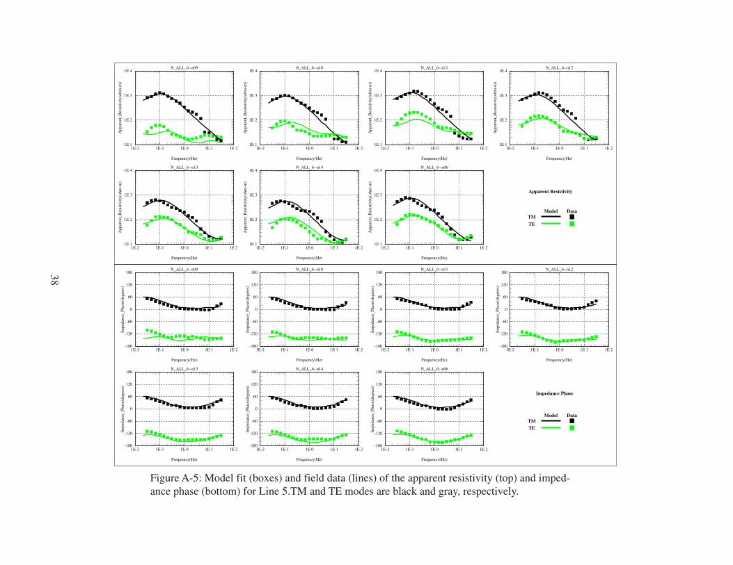
38

Figure A-5: Model fit (boxes) and field data (lines) of the apparent resistivity (top) and imped-ance phase (bottom) for Line 5.TM and TE modes are black and gray, respectively.

1E-2 1E-1 1E 0 1E 1 1E 2

Frequency(Hz)

N_ALL_6--n10

1E 1

1E 2

1E 3

1E 4

App

aren

t_R

esis

tivity

(ohm

-m)

1E-2 1E-1 1E 0 1E 1 1E 2

Frequency(Hz)

N_ALL_6--n14

1E 1

1E 2

1E 3

1E 4

App

aren

t_R

esis

tivity

(ohm

-m)

1E-2 1E-1 1E 0 1E 1 1E 2

Frequency(Hz)

N_ALL_6--n11

1E 1

1E 2

1E 3

1E 4

App

aren

t_R

esis

tivity

(ohm

-m)

1E-2 1E-1 1E 0 1E 1 1E 2

Frequency(Hz)

N_ALL_6--n06

1E 1

1E 2

1E 3

1E 4

App

aren

t_R

esis

tivity

(ohm

-m)

1E-2 1E-1 1E 0 1E 1 1E 2

Frequency(Hz)

N_ALL_6--n12

1E 1

1E 2

1E 3

1E 4

App

aren

t_R

esis

tivity

(ohm

-m)

1E-2 1E-1 1E 0 1E 1 1E 2

Frequency(Hz)

N_ALL_6--n09

1E 1

1E 2

1E 3

1E 4

App

aren

t_R

esis

tivity

(ohm

-m)

1E-2 1E-1 1E 0 1E 1 1E 2

Frequency(Hz)

N_ALL_6--n13

1E 1

1E 2

1E 3

1E 4

App

aren

t_R

esis

tivity

(ohm

-m)

1E-2 1E-1 1E 0 1E 1 1E 2

Frequency(Hz)

N_ALL_6--n10

-180

-120

-60

0

60

120

180

Impe

danc

e_Ph

ase(

degr

ees)

1E-2 1E-1 1E 0 1E 1 1E 2

Frequency(Hz)

N_ALL_6--n14

-180

-120

-60

0

60

120

180

Impe

danc

e_Ph

ase(

degr

ees)

1E-2 1E-1 1E 0 1E 1 1E 2

Frequency(Hz)

N_ALL_6--n11

-180

-120

-60

0

60

120

180

Impe

danc

e_Ph

ase(

degr

ees)

1E-2 1E-1 1E 0 1E 1 1E 2

Frequency(Hz)

N_ALL_6--n06

-180

-120

-60

0

60

120

180Im

peda

nce_

Phas

e(de

gree

s)

1E-2 1E-1 1E 0 1E 1 1E 2

Frequency(Hz)

N_ALL_6--n12

-180

-120

-60

0

60

120

180

Impe

danc

e_Ph

ase(

degr

ees)

1E-2 1E-1 1E 0 1E 1 1E 2

Frequency(Hz)

N_ALL_6--n09

-180

-120

-60

0

60

120

180

Impe

danc

e_Ph

ase(

degr

ees)

1E-2 1E-1 1E 0 1E 1 1E 2

Frequency(Hz)

N_ALL_6--n13

-180

-120

-60

0

60

120

180

Impe

danc

e_Ph

ase(

degr

ees)

DataTMTE

Model

DataTMTE

Model

Apparent Resistivity

Impedance Phase

39

Figure A-6: Model fit (boxes) and field data (lines) of the apparent resistivity (left) and imped-ance phase (right) for Line 6. TM and TE modes are black and gray, respectively.

1E-2 1E-1 1E 0 1E 1 1E 2

Frequency(Hz)

L7_ALL_NO_101--s17

1E 1

1E 2

1E 3

1E 4

App

aren

t_R

esis

tivity

(ohm

-m)

1E-2 1E-1 1E 0 1E 1 1E 2

Frequency(Hz)

L7_ALL_NO_101--s16

1E 1

1E 2

1E 3

1E 4A

ppar

ent_

Res

istiv

ity(o

hm-m

)

1E-2 1E-1 1E 0 1E 1 1E 2

Frequency(Hz)

L7_ALL_NO_101--s15

1E 1

1E 2

1E 3

1E 4

App

aren

t_R

esis

tivity

(ohm

-m)

1E-2 1E-1 1E 0 1E 1 1E 2

Frequency(Hz)

L7_ALL_NO_101--s25

1E 1

1E 2

1E 3

1E 4

App

aren

t_R

esis

tivity

(ohm

-m)

1E-2 1E-1 1E 0 1E 1 1E 2

Frequency(Hz)

L7_ALL_NO_101--s26

1E 1

1E 2

1E 3

1E 4

App

aren

t_R

esis

tivity

(ohm

-m)

1E-2 1E-1 1E 0 1E 1 1E 2

Frequency(Hz)

L7_ALL_NO_101--s23

1E 1

1E 2

1E 3

1E 4

App

aren

t_R

esis

tivity

(ohm

-m)

1E-2 1E-1 1E 0 1E 1 1E 2

Frequency(Hz)

L7_ALL_NO_101--s22

1E 1

1E 2

1E 3

1E 4

App

aren

t_R

esis

tivity

(ohm

-m)

1E-2 1E-1 1E 0 1E 1 1E 2

Frequency(Hz)

L7_ALL_NO_101--s21

1E 1

1E 2

1E 3

1E 4

App

aren

t_R

esis

tivity

(ohm

-m)

1E-2 1E-1 1E 0 1E 1 1E 2

Frequency(Hz)

L7_ALL_NO_101--s20

1E 1

1E 2

1E 3

1E 4

App

aren

t_R

esis

tivity

(ohm

-m)

1E-2 1E-1 1E 0 1E 1 1E 2

Frequency(Hz)

L7_ALL_NO_101--s18

1E 1

1E 2

1E 3

1E 4

App

aren

t_R

esis

tivity

(ohm

-m)

1E-2 1E-1 1E 0 1E 1 1E 2

Frequency(Hz)

L7_ALL_NO_101--s19

1E 1

1E 2

1E 3

1E 4

App

aren

t_R

esis

tivity

(ohm

-m)

1E-2 1E-1 1E 0 1E 1 1E 2

Frequency(Hz)

L7_ALL_NO_101--s17

-180

-120

-60

0

60

120

180

Impe

danc

e_Ph

ase(

degr

ees)

1E-2 1E-1 1E 0 1E 1 1E 2

Frequency(Hz)

L7_ALL_NO_101--s16

-180

-120

-60

0

60

120

180

Impe

danc

e_Ph

ase(

degr

ees)

1E-2 1E-1 1E 0 1E 1 1E 2

Frequency(Hz)

L7_ALL_NO_101--s15

-180

-120

-60

0

60

120

180

Impe

danc

e_Ph

ase(

degr

ees)

1E-2 1E-1 1E 0 1E 1 1E 2

Frequency(Hz)

L7_ALL_NO_101--s25

-180

-120

-60

0

60

120

180

Impe

danc

e_Ph

ase(

degr

ees)

1E-2 1E-1 1E 0 1E 1 1E 2

Frequency(Hz)

L7_ALL_NO_101--s26

-180

-120

-60

0

60

120

180

Impe

danc

e_Ph

ase(

degr

ees)

1E-2 1E-1 1E 0 1E 1 1E 2

Frequency(Hz)

L7_ALL_NO_101--s23

-180

-120

-60

0

60

120

180

Impe

danc

e_Ph

ase(

degr

ees)

1E-2 1E-1 1E 0 1E 1 1E 2

Frequency(Hz)

L7_ALL_NO_101--s22

-180

-120

-60

0

60

120

180

Impe

danc

e_Ph

ase(

degr

ees)

1E-2 1E-1 1E 0 1E 1 1E 2

Frequency(Hz)

L7_ALL_NO_101--s21

-180

-120

-60

0

60

120

180

Impe

danc

e_Ph

ase(

degr

ees)

1E-2 1E-1 1E 0 1E 1 1E 2

Frequency(Hz)

L7_ALL_NO_101--s20

-180

-120

-60

0

60

120

180

Impe

danc

e_Ph

ase(

degr

ees)

1E-2 1E-1 1E 0 1E 1 1E 2

Frequency(Hz)

L7_ALL_NO_101--s18

-180

-120

-60

0

60

120

180

Impe

danc

e_Ph

ase(

degr

ees)

DataTMTE

ModelData

TMTE

Model

Apparent Resistivity Impedance Phase

1E-2 1E-1 1E 0 1E 1 1E 2

Frequency(Hz)

L7_ALL_NO_101--s19

-180

-120

-60

0

60

120

180

Impe

danc

e_Ph

ase(

degr

ees)