Magnetic dipole and thermal radiation impacts on stagnation point flow of micropolar basednanofluids over a vertically stretching sheetFinite element approachKhan, Shahid Ali; Ali, Bagh; Eze, Chika; Lau, Kwun Ting; Ali, Liaqat; Chen, Jingtan; Zhao,Jiyun

Published in:Processes

Published: 01/07/2021

Document Version:Final Published version, also known as Publisher’s PDF, Publisher’s Final version or Version of Record

License:CC BY

Publication record in CityU Scholars:Go to record

Published version (DOI):10.3390/pr9071089

Publication details:Khan, S. A., Ali, B., Eze, C., Lau, K. T., Ali, L., Chen, J., & Zhao, J. (2021). Magnetic dipole and thermal radiationimpacts on stagnation point flow of micropolar based nanofluids over a vertically stretching sheet: Finite elementapproach. Processes, 9(7), [1089]. https://doi.org/10.3390/pr9071089

Citing this paperPlease note that where the full-text provided on CityU Scholars is the Post-print version (also known as Accepted AuthorManuscript, Peer-reviewed or Author Final version), it may differ from the Final Published version. When citing, ensure thatyou check and use the publisher's definitive version for pagination and other details.

General rightsCopyright for the publications made accessible via the CityU Scholars portal is retained by the author(s) and/or othercopyright owners and it is a condition of accessing these publications that users recognise and abide by the legalrequirements associated with these rights. Users may not further distribute the material or use it for any profit-making activityor commercial gain.Publisher permissionPermission for previously published items are in accordance with publisher's copyright policies sourced from the SHERPARoMEO database. Links to full text versions (either Published or Post-print) are only available if corresponding publishersallow open access.

Take down policyContact lbscholars@cityu.edu.hk if you believe that this document breaches copyright and provide us with details. We willremove access to the work immediately and investigate your claim.

Download date: 13/03/2022

processes

Article

Magnetic Dipole and Thermal Radiation Impacts on StagnationPoint Flow of Micropolar Based Nanofluids over a VerticallyStretching Sheet: Finite Element Approach

Shahid Ali Khan 1, Bagh Ali 2 , Chiak Eze 1 , Kwun Ting Lau 1, Liaqat Ali 3 , Jingtan Chen 1 and Jiyun Zhao 1,*

Citation: Khan, S.A.; Ali, B.; Eze, C.;

Lau, K.T.; Ali, L.; Chen, J.; Zhao, J.

Magnetic Dipole and Thermal

Radiation Impacts on Stagnation

Point Flow of Micropolar Based

Nanofluids over a Vertically

Stretching Sheet: Finite Element

Approach. Processes 2021, 9, 1089.

https://doi.org/10.3390/pr9071089

Academic Editor:Václav Uruba

Received: 9 May 2021

Accepted: 11 June 2021

Published: 23 June 2021

Publisher’s Note: MDPI stays neutral

with regard to jurisdictional claims in

published maps and institutional

affiliations.

Copyright: © 2021 by the authors.

Licensee MDPI, Basel, Switzerland.

This article is an open access article

distributed under the terms and

conditions of the Creative Commons

Attribution (CC BY) license (https://

creativecommons.org/licenses/by/

4.0/).

1 Department of Mechanical Engineering, City University of Hong Kong, Hong Kong, China;alikhan-c@my.cityu.edu.hk (S.A.K.); ezechikauofb@gmail.com (C.E.); kwuntlau4-c@my.cityu.edu.hk (K.T.L.);jingtchen6-c@my.cityu.edu.hk (J.C.)

2 School of Mathematics and Statistics, Northwestern Polytechnical University, Xi’an 710129, China;baghalisewag@mail.nwpu.edu.cn

3 School of Energy and Power, Xi’an Jiaotong University, Xi’an 710049, China; math1234@stu.xjtu.edu.cn* Correspondence: jiyuzhao@cityu.edu.hk

Abstract: An analysis for magnetic dipole with stagnation point flow of micropolar nanofluids ismodeled for numerical computation subject to thermophoresis, multi buoyancy, injection/suction,and thermal radiation. The partial derivative is involved in physical consideration, which is trans-formed to format of ordinary differential form with the aid of similarity functions. The variationalfinite element procedure is harnessed and coded in Matlab script to obtain the numerical solution ofthe coupled non-linear ordinary differential problem. The fluid temperature, velocity, tiny particlesconcentration, and vector of micromotion are studied for two case of buoyancy (assisting 0 < λ, andopposing 0 > λ) through finite-element scheme. The velocity shows decline against the rising offerromagnetic interaction parameter (β) (assisting 0 < λ and opposing 0 > λ), while the inversebehaviour is noted in micro rotation profile. Growing the thermo-phoresis and microrotation pa-rameters receded the rate of heat transfer remarkable, and micromotion and fluid velocity enhancedirectly against buoyancy ratio. Additionally, the rate of couple stress increased against rising ofthermal buoyancy (λ) and boundary concentration (m) in assisting case, but opposing case showsinverse behavior. The finite element scheme convergency was tested by changing the mesh size, andalso test the validity with available literature.

Keywords: micropolar ferromagnetic fluid; finite element method; nanofluid; thermal radiation;magnetic dipole

1. Introduction

Ferrofluids are the suspension of nanoscale ferromagnetic particles in fluid carrierand magnetized by the influence of magnetic field [1]. In recent years, the investigationon ferromagnetic fluids (FF) has also become interested due to wide application in thefield of chemical engineering, bio-medicine, nuclear power plants, robotics, compounds,micro-electro-mechanical, melted metals refinement, pumps, colored stains, X-ray machine,and shock absorbers, etc. [2,3]. In 1965, Stephen [4] pioneered the concept of ferrofluids(FF). This type of hybrid fluids is actually, a suspension of colloidal ferromagnetic particles(10 nm) in a base liquid. In the presence of a magnetic field, these fluids exhibit magne-tization to avoid their possible settling. In medical sciences, pain relief is managed withmagnet therapy. Electromechanical devices such as recording procedures and generatorsare associated with magnet interactions. Furthermore, these fluids are used in enhancingthe heat transfer rate. The study of ferromagnetic impacts in a liquid metal was initiallyconsidered by Albrecht et al. [5]. Anderson and Valnes [6] presented fundamentals offerromagnetic fluid flow. Shliomis [7] established the basic analytical models concerningto the motion of ferrofluids. Neuringer and Rosensweig [8] developed a formulation for

Processes 2021, 9, 1089. https://doi.org/10.3390/pr9071089 https://www.mdpi.com/journal/processes

Processes 2021, 9, 1089 2 of 19

the impact of magnetic body force with a consideration that the magnetic field is parallelto magnetization. Magnetization being temperature dependent, such a thermomagneticcoupling may result in various practical applications of ferrofluids (see [9]).

Fluids with microstructures are micropolar fluids [10]. Stiff randomly oriented parti-cles make up micropolar fluids. Some physical specimens of micropolar flow are liquidcrystals, blood flow, bubby liquids. The basic concepts of micropolar fluid, with someapplications in engineering, was firstly described in (1966) by Eringen [11]. From recentdecades, the interest of researchers in the theory of micropolar fluids have a significantlyenlarged cause of its immense applications in industrial and engineering fields such aspolymeric and colloids deferments, liquid crystal, liquid minerals, body fluids, enginelubricants, paint rheology, cervical flow, and thrust bearing technology [12,13]. The steadymicropolar based fluid passed through impermeable and permeable sheets was investi-gated by Hassanien et al. [14]. The heat transfer of micropolar fluid flow was studiedby Turkyilmazoglu [15]. The multi slips effects on dynamics of magnetohydrodynamicmicropolar based tiny particles suject to heat source were investigated by Sohaib et al. [16].

Several analysts have considered a continuously extending surface to study of bound-ary layer flow in recent decades because of its numerous applications in engineeringand industry [17,18]. Some applications are: paper production, metal-spinning, crystalsheets productions, drawing of plastic films, polymer dispensation of chemical engineeringplants, and coating of cable, etc. Crane’s [19] groundbreaking work examined the steadyflow through the linearly stretching plate. To study the influence of viscous and suction,Faraz et al. [20] examined the an axisymmetric geometry flow on the shrinking surface. Theeffects of injection/suction subject to mass and heat transfer over an extending sheet werediscussed in Gupta [21]. The point on the surface of object in the field of flow where thefluid is brought at rest by the object is called stagnation point. The magneto hydrodynamicsstagnation point flows with heat transfer effects are important in both practice and theory.Some practical applications include liquid crystals, blood flow, the aerodynamics extrusionof plastic sheets, the cooling of an infinite metallic plate in a cooling bath and textile andpaper industries [22,23]. Many researchers have deliberated the stagnation point flow overa stretching sheet [24,25]. Chiam [26] studied a two-dimensional stagnation point flow ofviscous fluid over a linearly stretching surface. Amjad et al. [27] examined the Cassonmicropolar based tiny particles flow in the stagnation point zone over a curved surface.

A designed fluid that can be utilized in the advanced technological areas with enor-mous diffusivity heat capacity is called nanofluid. Nanotechnology has recently piquedthe interest of many scientists due to its widespread use in industry as a result of nano-sized particles possessing a wide range of chemical and physical properties [28,29]. Thetiny particles made by nanomaterials are generally utilized as a coolant in mechanical,industrial, and chemical fields [30], and are utilized in various assembling applications,for example, cooking handling, cool, vehicle radiators, waste heat recovery, refrigeration,and so forth [31]. To begin, Choi [32] introduced the nanofluid in 1995, and he introducea fluid with tiny particles whose size less than (100nm) diameter. Vehicle cooling, fuelcells, lubricants, heat exchangers, cancer therapy, and micro-electro-mechanical structuresare just a few of the applications for heat transfer and nanofluid boundary layer flow inscience and engineering [33,34]. As a result, many researchers have experimented withand analyzed the flow and heat transfer physiognomies of nanofluids. Unsteady boundarylayer flow of nanofluids through a penetrable shrinking/stretching sheet was observed byBachok et al. [35]. Wen [36] speaks to the lacking minding of the structure and componentof nanofluids and furthermore their applications. The brownian motion of tiny particlesenhanced the host fluid heat transfer rate reported by Rasheed et el. [37] and Ali et al. [38].More work on nanofluid subject to various types of flow geometry is carried out [39–41].

The first aim of the current examination is to research the conduct of magnetic dipolealong with the stagnation point flow of micropolar based nanofluid over a vertical stretch-ing surface. Because of the complexity of technological processes, a quest for enhancebase fluid thermal efficacy is the rising research zone. The model of nanofluid has created

Processes 2021, 9, 1089 3 of 19

enough capacity to meet the growing demands. The majority of previous studies usedsimple fluids (water base fluid), but there exist non-Newtonian fluid that are more viscousin practice. The conduct of the involved parameters is exhibited graphically by a precisediscussion. Besides, the graphical portrayal of the Nusselt number, skin friction coefficient,and the Sherwood number coefficient is discussed. Furthermore, with Matlab coding, themost powerful finite element based computation carried out, and also test the accuracyand convergence of finite element scheme.

2. Mathematical Formulation (Magnetization+)

Consider two dimensional, steady, and incompressible flow acceleration because of avertical positioned surface, and fluid is contemplated across 0 < y there in pictographicdepiction Figure 1 in allusion to the OXY-Coordinate system. We presumed a stagnation-point flow of 2-D incompressible micropolar nanofluid across the surface. The surface ispresumed to be stretched with velocity Uw = ax and ue(x) = cx (external flow or freestream) is the flow rate away from the boundary layer and is assumed to be the hot fluidalong side the −κ f (

∂T∂y ) = h f (Tf − T) vertical wall. The magnet dipole is centered outside

the liquid at a distance b, with its core at (0,b) on the y-axis and the magnet field pointingalong the positive x-axis. It is stated that, T is the temperature of fluid, and Tc is a curietemperature often more appropriate as compared to Tw (wall surface temperature), whereasthe acoustic fluid temperature far from the sheet is T∞ = Tc, but there is no more magneticflux there until the magnetic nanofluid exceeds to Curie temperature Tc. The condensedstructure of the system of equations has predicated from the above assumptions havingboundary layer evaluations are (see [42,43]):

∂u∂x

+∂v∂y

= 0, (1)

u∂u∂x

+ v∂u∂y

= ue∂ue

∂x+

µ0

ρM

∂H∂x

+ (µ f + κ

ρ f)

∂2u∂y2 +

κ

ρ f

∂w∂y

+g

ρ f

[ρ f βt(T − T∞)(1− C∞) + βc(ρp − ρ f∞)(C− C∞)

], (2)

u∂w∂x

+ v∂w∂y

=γ f

(ρ f )j∂2w∂y2 −

κ

(ρ f )j(2w +

∂u∂y

), (3)

u∂T∂x

+ v∂T∂y

+

(u

∂H∗

∂x+ v

∂H∗

∂y

)µ0T

∂M∂T

= α∂2T∂y2 −

∂qr

∂y+ τ

(DT

T∞

(∂T∂y

)2

+ DB∂T∂y

∂C∂y

), (4)

u∂C∂x

+ v∂C∂y

= Ds∂2C∂y2 +

DT

T∞

(∂2T∂y2

). (5)

where, u, v are the velocity components in x, y directions, respectively, C, T are the tinyparticles’ volume concentration and fluid temperature, respectively, DB, DT , g∗, βT , βc, andare the Brownian diffusion, thermophoretic diffusion coefficient, gravitational acceleration,the thermal, and nanoparticle volume concentration expansion coefficient, respectively.τ∗ = (ρc)p/(ρc) f is the ratio of the nanoparticle material’s effective heat capacity to theheat capacity of the fluid. The spin gradient viscosity γ = (µj + κ

2 j) = µ f (j + K2 j) was

assumed by Khan et al. [44], where the material parameter is denoted by K = κµ In

addition, the intensity of the fluid is ρ, thermal diffusion α, viscosity κ, micro-inertia j, andω is the angular velocity, respectively. The radiation heat flux is defined below [45]:

qr =43

α∗

K1

∂T4

∂y2

Processes 2021, 9, 1089 4 of 19

uw

Cw

Tw

Buoyancy assisting region

Buoyancy opposing region

x

y

Nanoparticles

Ho

t co

nvectio

n flu

id

-ĸ

T/

y =

hf(

Tf-

T)

b

T

C

ue

v

u

g

Figure 1. Physical Configuration in xy-domain.

The Roseland mean coefficient of absorption is K1, whereas the Stefan Boltzmanconstant is α∗. Slight temperature variations in a flow are taken into consideration, andthus the Taylor series has been used to neglect higher-order terms; the result is

∂qr

∂y=−16α∗T3

∞3K1

∂2T∂y2

The respective boundary parameters of the preceding problem are

u− Uw(x) = ax, v− vw = 0, ω = −m∂u∂y

, κ f (∂T∂y

) = (h f T f − h f T), C = Cw(x), as y = 0, (6)

u→ ue = cx, ω → 0, T → T∞, C → C∞, as y→ ∞. (7)

where Tf denotes temperature and Cw represents the nano-particle’s concentration at thesurface. T∞ and C∞ are the corresponding ambient values. The m parameter is a boundaryconstant parameter with a value of 0 ≤ m ≤ 1. As m = 0, the microelements cannot rotate,ω = 0 takes place on the surface, 0.5 = m correlates the antisymmetric components of stresstensor vanishing, and 1.0 = m coincides turbulent flow of boundary layer. The progressionof magnetic ferrofluid is influenced by the magnetic field, because the magnetic dipolewith magnetic scalar potential is denoted as (see [46,47]):

Ψ =γ∗

2π

(x

x2 + (y + b)2

)(8)

After that, γ∗ stand for strength of magnetic field, and magnetic field amplitudesbesides the x and y-axis are written as:

H∗x = −∂Ψ∂x

=γ∗

2π

(x2 − (y2 + b2 + 2yb)(x2 + (y + b)2)2

), (9)

H∗y = −∂Ψ∂y

=γ∗

2π

(2xy + 2xb)

(x2 + (y + b)2)2

). (10)

Processes 2021, 9, 1089 5 of 19

Since the magnetic force is proportional to the slope of H. The corresponding magni-tude H of the magnetic field strength is described as follows

H∗ =[(

∂Ψ∂x

)2 + (∂Ψ∂y

)2] 1

2, (11)

∂H∗

∂x= −

(2x

(y + b)4

)γ∗

2π, (12)

∂H∗

∂y= −

(−2

(y + b)3 +4x2

(y + b)5

)γ∗

2π. (13)

The conversion of M into magnetization can be assumed temperature as a linear function.

M = (Tc − T)β∗ (14)

for which β∗ represent the pyromagnetic coefficient constant. In whichever case, the fol-lowing point is critical for the ferrohydrodynamic partnership event: (i) the temperatureof fluid T is specific in comparison to the external magnetic field TC, and (ii) the externalmagnetic field is different from the bulk. Further, no need to magnetization, once obtainedthe TC. The physical universality is important in view of the extremely high Curie tem-perature of iron, which is 1043 K. The following similarity transforms are used to convertEquations (1)–(5) to ordinary differential form (see [48,49]):

ψ(η, ξ) = (µ

ρ)η f (ξ), θ(η, ξ) =

Tc − TTc − Tw

, η =

√cµ

ρx, ξ =

√cµ

ρy,

u =∂ψ

∂x= ax f ′(ξ), v = −∂ψ

∂y= −√

aν f (ξ), g =ω

ax

√ν

a.

(15)

The stream function, and dimensionless coordinates are represented by ψ, η, and ξ,respectively. Equations (2)–(7) are transformed into ODE’s using Equation (15)

(K + 1)d3 fdξ3 −

(d fdξ

)2

+ fd2 fdξ2 + K

dgdξ− 2βθ1

(ξ + γ)4 ± λ

(θ + Nrφ

)+ R2 = 0, (16)

(1 +K2)

d2gdξ2 + f

dgdξ− g

d fdξ− K

(2g +

d2 fdξ2

)= 0, (17)

1Pr

(1 + Rd)d2θ

dξ2 + fdθ

dξ+ Nb

dθ

dξ

dφ

dξ+ Nt

(dθ

dξ

)2

+2λ1β(θ1 − ε) f

Pr(ξ + γ)3 = 0, (18)

d2φ

dξ2 + Le fdφ

dξ+

NbNt

dθ

dξ= 0, (19)

f (ξ) = fw,d fdξ

= 1, g(ξ) = −md2 fdξ2 ,

dθ

dξ− Cθ(ξ) = −C, φ(ξ) = 1, at ξ = 0,

d fdξ→ R, g→ 0, θ(ξ)→ 0, φ(ξ)→ 0, as ξ → ∞.

(20)

The developing parameters in Equations (16)–(20) are defined as

Processes 2021, 9, 1089 6 of 19

K =κ

µ, Pr =

ν

α, Le =

ν

DB, Rd =

16σ∗T3∞

3k∗K, Nb = (τDBCw − τDBC∞)ν−1, Nt =

τDT(Tw − T∞)ν−1

T∞,

R2 =c2

a2 , fw = − vw√aν

, C = −h f

κ f

√ν

a, Grt =

gρ f ∞βt(1− C∞)(Tw − T∞)x3

ν2 , Rax =Uw(x)x

ν,

Grc =gβc(ρp − ρ f ∞)(Cw − C∞)x3

ν2 , Nr =βc(ρp − ρ f ∞)(Cw − C∞)

βtρ f (1− C∞)(Tw − T∞), λ =

Grt

Ra2x

, λ1 =cµ2

ρk(Tc − Tw),

β =γ∗ρµ0

2πµ2 k(Tc − Tw), γ = d√

cρ

µ,

and ε = Tc(Tc−Tw)

symbolizes a material’s parameter (K), Lewis number (Le), radiationparameter (Rd), thermophoresis parameter (Nt), Prandtl number (Pr), Brownian motionparameter (Nb), here R2 is the constant, suction/injection parameter ( fw), and Biot (C),thermal Grashof (Grt), solutal Grashof (Grc), local Renolds (Rax), Eckert (λ1) numbers.Moreover buoyancy ratio (Nr), mixed convection (λ), ferrohydrodynamic interaction (β)parameters, dimensionless distance(γ), and Curie temperature ratio (ε). Further to that,a similar intensity of unity is applied to both buoyancy and thermal forces, regardingthe positive values for cumulative buoyancy forces resulting in negative attributes andsupporting flow resulting in competing for flow.

The terms for skin friction coefficient, Nusselt number, and the Sherwood number areas follows

C f =τw

ρU2w/2, Nu =

xqw

κ(Tw − T∞), Shr =

xqm

DB(Cw − C∞). (21)

From which the skin friction tensor at the wall is τw =[κω + (µ + κ) ∂u

∂y

]y=0

, at the

wall, the heat fluxion is qw =[(κ + 16αT3

3κ ) ∂T∂y

]y=0

, and the fluxion of mass from the surface

qm =(

DB∂C∂y

)y=0

. With the help of Equation (10), the following can be obtained

12

C f Rex2 = (1 + (1−m)K) f ′′(0),

Rex−12 Nu = −(Rd + 1)θ′(0),

Rex−12 Shr = −φ′(0).

(22)

3. Numerical Procedure

The finite-element technique is notable to address different kinds of differential equa-tion. This technique include continuous piecewise approximation, which minimize thesize of error [50]. The crucial steps and an extraordinary portrayal of this strategy sketchedout by jyothi [51] and Reddy [52]. This technique is very productive tool described bythe experts and scientists to examine the complicated problems of engineering becauseof its simplicity and accuracy [53–55]. To solve the Equations (16)–(19) along boundaryCondition (20), we first consider:

d fdξ

= h, (23)

Using Equation (23), Equations (16)–(20) are converted to (24) to (28), and are given as

Processes 2021, 9, 1089 7 of 19

(K + 1)d2hdξ2 + f

dhdξ− h2 + K

dgdξ− 2βθ1

(ξ + γ)4 ± λ

(θ + Nrφ

)+ R2 = 0, (24)

(1 +K2)

d2gdξ2 + f

dgdξ− gh− K

(2g +

dhdξ

)= 0, (25)

1Pr

(1 + Rd)d2θ

dξ2 + fdθ

dξ+ Nb

dθ

dξ

dφ

dξ+ Nt

(dθ

dξ

)2

+2λ1β(θ1 − ε) f

Pr(ξ + γ)3 = 0, (26)

d2φ

dξ2 + Le fdφ

dξ+

NbNt

dθ

dξ= 0, (27)

h(ξ) = 1, f (ξ)− fw = 0, g(ξ) + (m)dhdξ

= 0, φ(ξ) = 1.0,dθ

dξ= −(C + Cθ(ξ)), at ξ = 0.0,

h→ R, g→ 0.0, θ(ξ)→ 0.0, φ(ξ)→ 0.0, as ξ → ∞.

(28)

The variational forms of Equations (23)–(27) subject to linear-element Ωξ = (ξ a, ξ a+1)are given below ∫ ξ a+1

ξ aw1

d fdξ− hdξ = 0, (29)∫ ξ a+1

ξ aw2

(K + 1)

d2hdξ2 + f

dhdξ− h2 + K

dgdξ− 2βθ1

(ξ + γ)4 ± λ

(θ + Nrφ + Rbγ

)+ R2

dξ = 0, (30)

∫ ξ a+1

ξ aw3

(1 +

K2)

d2gdξ2 + f

dgdξ− gh− K

(2g +

dhdξ

)dξ = 0, (31)

∫ ξ a+1

ξ aw4

1

Pr(1 + Rd)

d2θ

dξ2 + fdθ

dξ+ Nb

dθ

dξ

dφ

dξ+ Nt

(dθ

dξ

)2

+2λ1β(θ1 − ε) f

Pr(ξ + γ)3

dξ = 0, (32)

∫ ξ a+1

ξ aw5

d2φ

dξ2 + Le fdφ

dξ+

NbNt

dθ

dξ

dξ = 0. (33)

Here, w1, w2, w3, w4, and w5 are test functions. The associate approximations offinite-element are

f =p

∑j=1

f jψj, h =p

∑j=1

hjψj,dθ

dξ=

p

∑j=1

dθj

dξψj,

dφ

dξ=

p

∑j=1

dφj

dξψj. (34)

with w1 = w2 = w3 = w4 = w5 = ψj(j = 1, 2), here, ψj (j = 1,2) are the linear-interpolationfunctions and are given by

ψ1 =ξ a+1 − ξ

ξ a+1 − ξ a, ψ2 =

ξ − ξ a

ξ a+1 − ξ a, ξ a ≤ ξ ≤ ξ a+1. (35)

The model of finite elements of the equations thus developed is given by[W11] [W12] [W13] [W14] [W15][W21] [W22] [W23] [W24] [W25][W31] [W32] [W33] [W34] [W35][W41] [W42] [W43] [W44] [W45][W51] [W52] [W53] [W54] [W55]

f hgθφ

=

b1b2b3b4b5

(36)

where [Wmn] and [bm], (m, n = 1, 2, 3, 4, 5) are defined as:

Processes 2021, 9, 1089 8 of 19

W11ij =

∫ ξ a+1

ξ aψi

dψj

dξdξ, W12

ij = −∫ ξ a+1

ξ aψiψjdξ, W13

ij = W14ij = W15

ij = W21ij = 0,

W22ij = −(K + 1)

∫ ξ a+1

ξ a

dψidξ

dψj

dξdξ +

∫ ξ a+1

ξ af ψi

dψj

dξdξ −

∫ ξ a+1

ξ ahψiψjdξ, W23

ij = K∫ ξ a+1

ξ aψiψjdξ,

W24ij =

2β

(ξ + γ)4

∫ ξ a+1

ξ aψiψjdξ ± λ

∫ ξ a+1

ξ aψiψjdξ, W25

ij = Nr∫ ξ a+1

ξ aψiψjdξ,

W31ij = 0, W32

ij = −K∫ ξ a+1

ξ aψi

dψj

dξdξ, W33

ij = −(1 + K2)∫ ξ a+1

ξ a

dψidξ

dψj

dξdξ −

∫ ξ a+1

ξ ahψiψjdξ +

∫ ξ a+1

ξ af ψi

dψj

dξdξ

− 2K∫ ξ a+1

ξ aψiψjdξ, W34

ij = W35ij = 0, W41

ij = − 2λ1βε

Pr(ξ + γ3)

∫ ξ a+1

ξ aψiψjdξ, W42

ij = W43ij = 0,

W44ij = − 1

Pr(1 + Rd)

∫ ξa+1

ξa

dψidξ

dψj

dξdξ +

∫ ξa+1

ξaf ψi

dψj

dξdξ − Nb

∫ ξa+1

ξaφ′ψi

dψj

dξdξ + Nt

∫ ξa+1

ξaθ′ψi

dψj

dξdξ,

+2λ1β

Pr(ξ + γ3)

∫ ξ a+1

ξ af ψiψjdξW45

ij = W46ij = 0, W51

ij = W52ij = W53

ij = 0,

W54ij = − Nt

Nb

∫ ξa+1

ξa

dψidξ

dψj

dξdξ, W55

ij = −∫ ξa+1

ξa

dψidξ

dψj

dξdξ + Le

∫ ξa+1

ξaf ψi

dψj

dξdξ,

and

b1i = 0, b2

i = −(K + 1)(ψdhdξ

)ξa+1ξa− R2, b3

i = −(1 + K2)(ψ

dgdξ

)ξa+1ξa

b4i = − 1

Pr(1 + Rd)(ψ

dθ1

dξ)ξa+1

ξab5

i = −(ψ dφ

dξ)ξa+1

ξa− Nt

Nb(ψ

dθ

dξ)ξe+1

ξe. (37)

where the known values taken into account are f = ∑2j=1 f jψj, h = ∑2

j=1 hjψj, θ′ = ∑2j=1 θ′jψj,

and φ′ = ∑2j=1 φ′jψj. The whole domain (ξ = 10) is alienated into equal linear size elements

(n), and observe no further variation after 300 and 400, so the final results are computed at300 linear elements (see Table 1). Five functions were evaluated at each node, acquiring1505× 1505 non-linear equations after assembly, so the Gaussian quadrature method isused to solve the integration, attaining an accuracy level of 10−5.

Table 1. The finite element scheme convergence against a number of elements (n), when R = 1,Pr = 2, C = 0.5, Nb = 0.5, Nt = 0.5, Le = 2, K = 5, γ = 1.0, λ = 1, λ1 = 0.1, β = 0.2, ε = 0.5,Nr = 1, m = 0.5, fw = 0.2, Rd = 0.5

n f (3) h(3) g(3) θ(3) φ(3)

40 1.746747 1.028292 0.002454 0.036199 0.01787460 1.746657 1.028291 0.002451 0.036194 0.017859

100 1.746611 1.028289 0.002453 0.036191 0.017855130 1.746598 1.028289 0.002453 0.036191 0.017855200 1.746592 1.028289 0.002453 0.036190 0.017854300 1.746588 1.028289 0.002453 0.036190 0.017854400 1.746587 1.028289 0.002453 0.036190 0.017854

4. Results and Discussion

In present report, the calculations have been achieved for micro-rotation, tempera-ture, velocity, and tiny particles concentration distributions for involved parameters inEquations (16)–(20). To approve the present numerical technique Matlab code, an exten-sive comparison of results is made, as showed in Table 2–4, and are found to show anexcellent relationship between already existing outcomes. In the absence of all involved

Processes 2021, 9, 1089 9 of 19

physical parameters except R for skin friction factor is compared with Ishak et al. [56],Mahapatra et al. [57], Khan et al. [58], and Nazar et al. [59] against growing input of Ras represent in Table 2. The results of C f Re1/2

x and NuRe−1/2x for R and K at Pr = 1.5

are compared with Mahapatra et al. [57], Qasim et al. [60], and Tripathy et al. [61] (seeTables 2 and 3) when other involved parameters are zeros. Table 4 represents the numericaloutcomes of NuRe−1/2

x , and ShRe−1/2x for specific values of Nt by Qasim et al. [60], when

Nb = 0.1, Pr = 10.0, Le = 1.0, and not considered others involved parameters. Alongthese lines, trust in the present FEM calculations are very high. The default values of theparameters in the study are: Pr = 2, K = 5, m = ε = 0.5, β = 0.2, C = 0.5, λ = 1, Nr = 1,Le = 2, λ1 = 0.1, fw = 0.2, Nb = 0.5 Rd = 0.5, Nt = 0.5, R = 1, and γ = 1.

Table 2. Comparison of C f Re1/2x against R, when not considering other involved parameters.

R Ref. [56] Ref. [57] Ref. [58] Ref. [59] FEM(Current Outcomes)

0.1 −0.9694 −0.9694 −0.96938 −0.9694 −0.9693840.2 −0.9181 −0.9181 −0.91810 −0.9181 −0.9181040.5 −0.6673 −0.6673 −0.66726 −0.6673 −0.6672622.0 2.0175 2.0175 2.01750 2.0176 2.0175063.0 4.7294 4.7293 4.72928 4.7296 4.729308

Table 3. Comparison of C f Re1/2x and NuRe−1/2

x for various values of R and K, when Pr = 1.5 and not considering otherinvolved parameters.

K RRef. [57] Ref. [60] Ref. [61] FEM (Our Results)

NuRe−1/2x C f Re1/2

x C f Re1/2x C f Re1/2

x NuRe−1/2x

0.0 0.0 - −1.000000 −1.000172 −1.000006 −0.76027981.0 - - −1.367872 −1.367902 −1.367994 −0.82177142.0 - - −1.621225 −1.621938 −1.621573 −0.84954534.0 - - −2.004133 −2.007341 −2.005420 −0.87810490.0 0.1 −0.777 - - −0.969384 −0.7767970- 0.2 −0.797 - - −0.918104 −0.7971178- 0.5 −0.863 - - −0.667262 −0.8647908- 2.0 −1.171 - - 2.0175063 −1.1781084- 3.0 −1.341 - - 4.7293083 −1.3519641

Table 4. Comparison of NuRe−1/2x , and ShRe−1/2

x for specific values of Nt, when Nb = 0.1, Pr = 10.0,Le = 1.0, and not considering other involved parameters.

NtRef. [60] FEM (Our Results)

NuRe−1/2x ShRe−1/2

x NuRe−1/2x ShRe−1/2

x

0.1 0.9524 2.1294 0.952363 2.1293700.2 0.6932 2.2740 0.693164 2.2739990.3 0.5201 2.5286 0.520071 2.5286130.4 0.4026 2.7952 0.402574 2.7951410.5 0.3211 3.0351 0.321051 3.035102

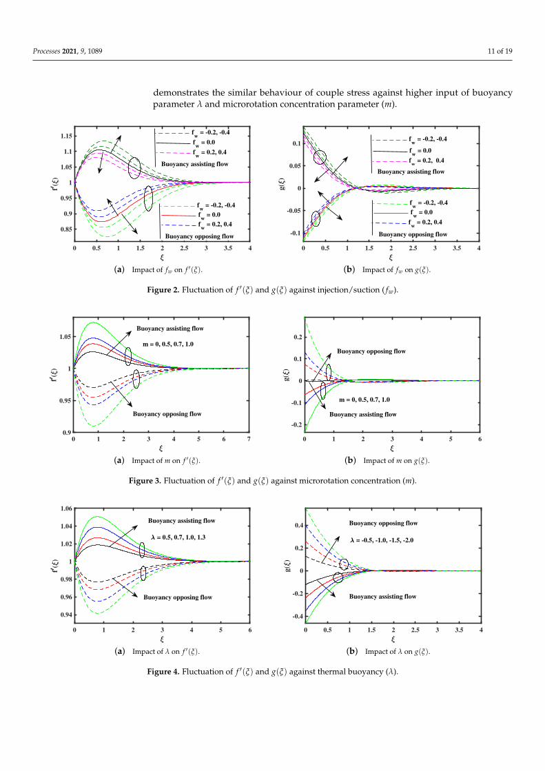
The Figure 2a demonstrates the influence of fw (suction/injection) on f ′(ξ) (flowvelocity). It can be seen that velocity of fluid rises against growing input of injection forthe case of buoyancy assisting flow, but it recede against rising in suction. However, foropposing flow situation, an inverse behaviour is noted against higher input of fw (suction/injection). A similar curves for g(ξ) (microrotation) are obtained against growing value offw, opposing /assisting flow has similar behaviour to that the velocity as demonstrated in

Processes 2021, 9, 1089 10 of 19

Figure 2b. Further, the conversion in velocity distribution is more prominent than that ofmicrorotation micro-rotation. The impacts of microrotation concentration parameter m onvelocity, and microrotation is exposed in Figure 3a,b. It can be visualized that for a steadyincrease of m, in the boundary layer region, the fluid velocity becomes faster (in case ofλ > 0), but slows down (in a case λ < 0). How the magnitude of micro-rotation exhibitdirectly proportional behaviour with a variation of m for both cases of λ (λ > 0 or λ < 0).However, reversal sping is noticed for λ < 0 viz-a-viz λ > 0. Figure 4a,b discloses that theelevation in the value of buoyancy parameter (λ > 0 or λ < 0) marked similar influence onf ′(ξ), and g(ξ) as the parameter m did on these quantities and described with reference ofFigure 3a,b above. Physically, growing values of λ provided larger buoyancy force, whichdiscloses the kinetic energy at the extreme level. Consequently, resistance produce in thedirection of flow because of kinetic energy. The opposite trend take place in microrotation(g(ξ)) via incremented λ. The growing input of λ exhibits the rising behaviour for opposingflow, and diminishing trend for assisting flow (see Figure 4b).

Figure 5a,b demonstrate the patterns of f ′(ξ) and g(ξ) when the Nr is increasinglyvaried. The observation reveals that flow is accelerated in the boundary layer when λ > 0,but retarded when λ < 0, and the magnitude of micro-rotation is directly enhanced withNr. One of the main interests of this work is to highlight the role of the magnet dipole,which is represented by parameter β in Figure 6a,b. As expected in the graphical pattern,the fluid velocity is significantly reduced for β (λ < 0 and λ > 0). The reason for thisis that the magnet dipole adds to the strength of the applied magnetic field. The stronginteraction of magnetic and electric fields results in the increase in Lorentz force, whichdelivers resistance to the flow (see Figure 6a). In part of Figure 6b one can notice thatincrements in β lead to a rise in micro-rotation g(ξ) for λ < 0, but this recedes for λ > 0.

Regarding their physical nature, the rising strength of Pr (Prandtl number) respondsto medium thermal diffusivity. A reduction in temperature function and nanoparticleconcentration distribution with the incremented value of Pr is shown in Figure 7a,b. Thethermal diffusivity intensifies with increasing of Pr values; as a consequence, the θ(ξ) andφ(ξ) functions exhibit a reduction. The responses of the temperature function and theconcentration distribution to the increasing Brownian motion Nb values are respectivelyshown in Figure 8a,b. It can be seen that the curve in θ(ξ) rises notably for both the of (λ > 0or λ < 0) prospects, but the φ(ξ) cure is declined in these circumstances. The randommotion of tiny particles is incremented because of Brownian motion, which enhances θ(ξ),and recedes the φ(ξ). Figure 9a,b is demonstrates the incremental trends and with steadyincrease in the thermophoresis parameter Nt. Physically, thermophoresis (Nt) exert forceover neighbouring tinyparticles; the force changes the tiny particles from a hotter zone to acolder zone. Hence, φ(ξ) and θ(ξ) incremented because it exceeds Nt. The Biot numbersymbolized by C has had a similar impact as the thermophoresis parameter. The graphicaloutcomes for this aspect of the study are depicted in Figure 10a,b. The exceeding valuesof radiation Rd signify the increment in thermal transportation in the fluid. Figure 11ashows that the rise in temperature function and thermal boundary layers becomes widerwith higher Rd values, but a meager reduction in nanoparticle volume fraction is plottedin Figure 11b.

The deviation in Sherwood and Nusselt numbers for different input of the Nt andK is investigated individually in Figure 12a,b. It is clearly seen that 0 < λ and 0 > λreduces steadily the Nusselt number via the larger Nt, and K (microrotation parameter).Nonetheless, the mass gradient (Sherwood number) denoted an expanding pattern againstthe growing of K, however it exhibits a diminishing behaviour vesus Nt. Figure 13a,bindividually portray the Nusselt and Sherwood numbers as affected by λ, and K. Fromthese sketch, it is clearly observed that λ > 0 (buoyancy assisting flow), the Sherwood andNusselt numbers demonstrate a decline against exceeding of K. Figure 14a portrays theskin friction factor against higher estimation of λ and K. From this sketch designs, onecan be seen that assisting case (λ > 0), the exceeding input of K responsible of growingskin friction factor, and an opposite trend is seen against λ < 0. Similarly, Figure 14b

Processes 2021, 9, 1089 11 of 19

demonstrates the similar behaviour of couple stress against higher input of buoyancyparameter λ and microrotation concentration parameter (m).

0 0.5 1 1.5 2 2.5 3 3.5 4

0.85

0.9

0.95

1

1.05

1.1

1.15

f(

)

fw

= -0.2, -0.4

fw

= 0.0

fw

= 0.2, 0.4

fw

= -0.2, -0.4

fw

= 0.0

fw

= 0.2, 0.4

Buoyancy opposing flow

Buoyancy assisting flow

(a) Impact of fw on f ′(ξ).

0 0.5 1 1.5 2 2.5 3 3.5 4

-0.1

-0.05

0

0.05

0.1

g(

)

fw

= -0.2, -0.4

fw

= 0.2, 0.4

fw

= 0.0

Buoyancy assisting flow

fw

= -0.2, -0.4

fw

= 0.0

fw

= 0.2, 0.4

Buoyancy opposing flow

(b) Impact of fw on g(ξ).

Figure 2. Fluctuation of f ′(ξ) and g(ξ) against injection/suction ( fw).

0 1 2 3 4 5 6 70.9

0.95

1

1.05

f(

)

Buoyancy assisting flow

m = 0, 0.5, 0.7, 1.0

Buoyancy opposing flow

(a) Impact of m on f ′(ξ).

0 1 2 3 4 5 6

-0.2

-0.1

0

0.1

0.2

g(

)

Buoyancy assisting flow

m = 0, 0.5, 0.7, 1.0

Buoyancy opposing flow

(b) Impact of m on g(ξ).

Figure 3. Fluctuation of f ′(ξ) and g(ξ) against microrotation concentration (m).

0 1 2 3 4 5 6

0.94

0.96

0.98

1

1.02

1.04

1.06

f(

)

Buoyancy assisting flow

Buoyancy opposing flow

= 0.5, 0.7, 1.0, 1.3

(a) Impact of λ on f ′(ξ).

0 0.5 1 1.5 2 2.5 3 3.5 4

-0.4

-0.2

0

0.2

0.4

g(

)

Buoyancy opposing flow

= -0.5, -1.0, -1.5, -2.0

Buoyancy assisting flow

(b) Impact of λ on g(ξ).

Figure 4. Fluctuation of f ′(ξ) and g(ξ) against thermal buoyancy (λ).

Processes 2021, 9, 1089 12 of 19

0 1 2 3 4 5 6

0.96

0.98

1

1.02

1.04

f(

)

Buoyancy opposing flow

Buoyancy assisting flow

Nr = 0, 0.5, 0.7, 1.0

(a) Impact of Nr on f ′(ξ).

0 1 2 3 4 5 6

-0.06

-0.04

-0.02

0

0.02

0.04

0.06

g(

)

Buoyancy opposing flow

Buoyancy assisting flow

Nr = 0, 0.5, 0.7, 1.0

(b) Impact of Nr on g(ξ).

Figure 5. Fluctuation of f ′(ξ) and g(ξ) against buoyancy ratio (Nr).

0 1 2 3 4 5 6 7

0.94

0.96

0.98

1

1.02

1.04

f(

)

Buoyancy assisting flow

Buoyancy opposing flow

= 0.5, 1.0, 1.5, 2.0

(a) Impact of β on f ′(ξ).

0 1 2 3 4 5 6

-0.05

0

0.05

0.1

g(

)

Buoyancy opposing flow

Buoyancy assisting flow

= 0.5, 1.0, 1.5, 2.0

(b) Impact of β on g(ξ).

Figure 6. Fluctuation of f ′(ξ) and g(ξ) against ferrohydrodynamic interaction (β).

0 0.5 1 1.5 2 2.5 3 3.5 40

0.1

0.2

0.3

0.4

()

Buoyancy assisting flow

Buoyancy opposing flow

Pr = 1.0

Pr = 1.5

Pr = 2.0

Pr = 3.0

Pr = 1.0Pr = 1.5

Pr = 2.0

Pr = 3.0

(a) Impact of Pr on θ(ξ). (b) Impact of Pr on φ(ξ).

Figure 7. Fluctuation of θ(ξ) and φ(ξ) against Prandtl number (Pr).

Processes 2021, 9, 1089 13 of 19

0 0.5 1 1.5 2 2.5 30

0.1

0.2

0.3

0.4

0.5

()

Nb = 0.3

Nb = 0.5

Nb = 0.7Nb = 1.0

Nb = 0.3Nb = 0.5

Nb = 0.7

Nb = 1.0

Buoyancy assisting flow

Buoyancy opposing flow

(a) Impact of Nb on θ(ξ).

0 0.5 1 1.5 2 2.50

0.2

0.4

0.6

0.8

1

()

Buoyancy opposing flow

Buoyancy assisting flow

Nb = 1.0

Nb = 0.7

Nb = 0.5Nb = 0.3

Nb = 1.0Nb = 0.7

Nb = 0.5

Nb = 0.3

(b) Impact of Nb on φ(ξ).

Figure 8. Fluctuation of θ(ξ) and φ(ξ) against Brownian motion (Nb).

0 0.5 1 1.5 2 2.50

0.1

0.2

0.3

0.4

()

Nt = 0.3

Nt = 0.5

Nt = 0.7

Nt = 1.0

Nt = 0.3Nt = 0.5

Nt = 0.7

Nt = 1.0

Buoyancy assisting flow

Buoyancy opposing flow

(a) Impact of Nt on θ(ξ).

0 0.5 1 1.5 2 2.50

0.2

0.4

0.6

0.8

1(

)

Buoyancy opposing flow

Buoyancy assisting flow

Nt = 1.0

Nt = 0.7

Nt = 0.5Nt = 0.3

Nt = 1.0

Nt = 0.7

Nt = 0.5

Nt = 0.3

(b) Impact of Nt on φ(ξ).

Figure 9. Fluctuation of θ(ξ) and φ(ξ) against thermophoresis (Nt).

0 0.5 1 1.5 2 2.5 30

0.2

0.4

0.6

0.8

()

C = 0.7

C = 1.5

C = 2.5C = 3.5

C= 0.7C = 1.5

C = 2.5

C = 3.5

Buoyancy assisting flow

Buoyancy opposing flow

(a) Impact of C on θ(ξ).

0 0.5 1 1.5 2 2.50

0.2

0.4

0.6

0.8

1

() 0.92 1

0.06

0.08

0.1

0.12

()

C = 1.5

C = 0.7

C = 2.5C = 3.5

C= 0.7C = 1.5

C = 2.5

C = 3.5

Buoyancy assisting flow

Buoyancy opposing flow

(b) Impact of C on φ(ξ).

Figure 10. Fluctuation of θ(ξ) and φ(ξ) against Biot number (C).

Processes 2021, 9, 1089 14 of 19

0 0.5 1 1.5 2 2.5 3 3.5 40

0.1

0.2

0.3

0.4

0.5

()

Rd = 0.5

Rd = 1.0

Rd = 2.0

Rd = 3.0

Buoyancy assisting flow

Rd = 0.5Rd = 1.0

Rd = 2.0

Rd = 3.0

Buoyancy opposing flow

(a) Impact of Rd on θ(ξ). (b) Impact of Rd on φ(ξ).

Figure 11. Fluctuation of θ(ξ) and φ(ξ) against radiation (Rd).

0.2 0.3 0.4 0.5 0.6 0.7 0.8

Nt

0.38

0.4

0.42

0.44

0.46

0.48

0.5

0.52

0.54

Nu

Re

-1/2

x

K = 2.0

K = 3.0

K = 4.0K = 5.0

Buoyancy assisting flow

K = 2.0

K = 3.0K = 4.0

K = 5.0

Buoyancy opposing flow

(a) Impact of K and Nt on NuRe−1/2x .

0.2 0.3 0.4 0.5 0.6 0.7 0.8

Nt

1.5

1.6

1.7

1.8

1.9

2

2.1

2.2

Sh

rRe

-1/2

x

Buoyancy opposing flow

K = 5.0

K = 4.0K = 3.0

K = 2.0

Buoyancy assisting flow

K = 5.0K = 4.0

K = 3.0

K = 2.0

(b) Impact of K and Nt on ShrRe−1/2x .

Figure 12. Fluctuation of NuRe−1/2x and ShrRe−1/2

x against material parameter (K) and thermophoresis (Nt).

0 0.5 1 1.5 2 2.5 30.42

0.43

0.44

0.45

0.46

0.47

0.48

Nu

Re

-1/2

x

K = 2.0K = 3.0K = 4.0K = 5.0

K = 2.0K = 3.0K = 4.0

K = 5.0

Buoyancy assisting flow

Buoyancy opposing flow

(a) Impact of K and λ on NuRe−1/2x .

0 0.5 1 1.5 2 2.5 31.9

1.95

2

2.05

2.1

2.15

2.2

Sh

rRe

-1/2

x

K= 2.0K = 3.0K = 4.0K = 5.0

K = 2.0K = 3.0K = 4.0

K = 5.0

Buoyancy assisting flow

Buoyancy opposing flow

(b) Impact of K and λ on ShrRe−1/2x .

Figure 13. Fluctuation of NuRe−1/2x and ShrRe−1/2

x against material parameter (K) and thermal buoyancy (λ).

Processes 2021, 9, 1089 15 of 19

0 0.5 1 1.5 2 2.5 3-2

-1.5

-1

-0.5

0

0.5

1

1.5

1/2

Re

1/2

xC

f

1.8

-1.6

-1.4

1.7 1.8

1.1

1.2

1.3

K = 2.0

K = 2.0

Buoyancy assisting flow

K = 5.0K = 4.0K = 3.0

K = 5.0

K = 4.0

K = 3.0

Buoyancy opposing flow

(a) Impact of K and λ on 12 Rex

2C f .

0 0.5 1 1.5 2 2.5 3-2

-1.5

-1

-0.5

0

0.5

1

1.5

2

Re

1/2

xM

x

m = 0.0

m = 0.0

m = 1.0

Buoyancy assisting flow

m = 1.0m = 0.7m = 0.5

Buoyancy opposing flow

m = 0.5m = 0.7

(b) Impact of m and λ on Re1/2x Mx .

Figure 14. Fluctuation of 12 Rex

2C f and Re1/2x Mx against material parameter (K), microrotation concentration (m), and

thermal buoyancy (λ).

5. Conclusions

The impacts of magnetic dipole and multiple buoyancy on micropolar fluid subject totiny particles over a vertical extending surface are studied numerically by the Galaerikintechnique using the finite element approach. The remarkable findings are mentioned below:

• The velocity decelerate against the exceeding of ferromagnetic interaction parameterβ in both cases (opposing and assisting), while an opposite behavior is noted in microrotation g(ξ) profile.

• The micro rotation g(ξ) and velocity f ′(ξ) enhance against the rising of microrota-tion concentration (m), injection ( fw), and buoyancy forces(Rb, λ, Nr) parameters inassisting case, but the inverse behaviour is reported in opposing case.

• The microrotation and velocity reduce along growing of micropolar material, andsuction ( fw) parameters in case of assisting, but opposite phenomena is seen in caseof opposing.

• The distribution of temperature shows a rising along the growing of the Brownianmotion, thermophoresis, Biot number, and radiation parameters, while the tempera-ture declined with the elevation of Prandtl number, and rate of heat transfer is lowerin assisting case.

• The tiny particles concentration distribution φ(ξ) demonstrates a decrease alongthe raising of Prandtl number, and Brownian motion, while the non-dimensionalconcentration enhance with upgrading of radiation, Biot number, and thermophoresisparameters. Moreover, it is noted that the impact of opposing case on the non-dimensional concentration profile is high as compared to assisting case.

• The Sherwood and Nusselt numbers coefficient rate become smaller against higher Kin assisting case, but opposing case exhibit inverse trend, and decreased by mean ofrising λ in opposing case, but reverse phenomena is reported in assisting case.

• An increase in thermophoresis and material parameters, decline in Nusselt number isnoted, and Sherwood number show an opposite affects along elevation of K.

• The skin friction factor rise, by mean of growing λ and K in assisting case, but opposingcase exhibits an opposite trend. Additionally, the rate of couple stress increased againstrising of λ and m in assisting case, but opposing case shows inverse behavior.

Author Contributions: S.A.K. modeled the problem and wrote the manuscript. C.E. complete theformal analysis and revision. K.T.L. and L.A. thoroughly checked the mathematical modeling, Englishcorrections, forma analysis and revision. B.A. solved the problem using MATLAB software. J.C. andJ.Z.: writing—review and editing. All authors finalized the manuscript after its internal evaluation.All authors have read and agreed to the published version of the manuscript.

Processes 2021, 9, 1089 16 of 19

Funding: No funding information is available.

Institutional Review Board Statement: Not applicable.

Informed Consent Statement: Not applicable.

Data Availability Statement: Not applicable.

Conflicts of Interest: The authors declare no conflict of interest.

Nomenclature

T non-dimensional temperatureTc curie temperatureC non-dimensional nanoparticles concentrationCw Concentration at surfaceω micro-rotationg gravitational accelerationT∞ temperature away from the surfaceUw velocity of stretching sheetC∞ concentration away from the surfaceue free streamC f skin friction(u, v) Velocity componentsNu Nusselt numberµ f dynamic viscosityShr Sherwood numberκ vortex viscosity,Nb Brownian motion parameterγ spin gradient viscosityNt thermophoresis parameterρ Density of fluidDT Thermophoretic diffusion coefficientDB Brownian diffusion coefficientρCp Base fluid heat capacityα thermal diffusivityj micro-inertiaβt coefficient of thermal expansionβc coefficient of nanoparticle volumetricα∗ Stefan Boltzman constantb distanceβ∗ pyromagnetic coefficientβ ferrohydrodynamic interaction variableλ mixed convection variableε dimensionless Curie temperaturePr Prandtl numberfw suction/injectionRd radiation variableLe Lewis numberR2 constantλ1 Eckert numberC Biot numberRax local Renolds numberK material parameter.

Processes 2021, 9, 1089 17 of 19

References1. Hayat, T.; Ahmad, S.; Khan, M.I.; Alsaedi, A. Simulation of ferromagnetic nanomaterial flow of Maxwell fluid. Results Phys. 2018,

8, 34–40. [CrossRef]2. Godson, L.; Raja, B.; Lal, D.M.; Wongwises, S.E.A. Enhancement of heat transfer using nanofluids—An overview. Renew. Sustain.

Energy Rev. 2010, 14, 629–641. [CrossRef]3. Ali, L.; Liu, X.; Ali, B.; Mujeed, S.; Abdal, S.; Khan, S.A. Analysis of Magnetic Properties of Nano-Particles Due to a Magnetic

Dipole in Micropolar Fluid Flow over a Stretching Sheet. Coatings 2020, 10, 170. [CrossRef]4. Stephen, P.S. Low Viscosity Magnetic Fluid Obtained by the Colloidal Suspension of Magnetic Particles. U.S. Patent 3,215,572, 2

November 1965.5. Albrecht, T.; Bührer, C.; Fähnle, M.; Maier, K.; Platzek, D.; Reske, J. First observation of ferromagnetism and ferromagnetic

domains in a liquid metal. Appl. Phys. A 1997, 65, 215–220. [CrossRef]6. Andersson, H.; Valnes, O. Flow of a heated ferrofluid over a stretching sheet in the presence of a magnetic dipole. Acta Mech.

1998, 128, 39–47. [CrossRef]7. Shliomis, M. Comment on “ferrofluids as thermal ratchets”. Phys. Rev. Lett. 2004, 92, 1–6. [CrossRef]8. Neuringer, J.L.; Rosensweig, R.E. Ferrohydrodynamics. Phys. Fluids 1964, 7, 1927–1937. [CrossRef]9. Bailey, R. Lesser known applications of ferrofluids. J. Magn. Magn. Mater. 1983, 39, 178–182. [CrossRef]10. Mehmood, Z.; Mehmood, R.; Iqbal, Z. Numerical investigation of micropolar Casson fluid over a stretching sheet with internal

heating. Commun. Theor. Phys. 2017, 67, 443. [CrossRef]11. Eringen, A.C. Theory of micropolar fluids. J. Math. Mech. 1966, 16, 1–18. [CrossRef]12. Izadi, M.; Sheremet, M.A.; Mehryan, S.; Pop, I.; Öztop, H.F.; Abu-Hamdeh, N. MHD thermogravitational convection and thermal

radiation of a micropolar nanoliquid in a porous chamber. Int. Commun. Heat Mass Transf. 2020, 110, 104409. [CrossRef]13. Izadi, M.; Mohammadi, S.A.; Mehryan, S.; Yang, T.; Sheremet, M.A. Thermogravitational convection of magnetic micropolar

nanofluid with coupling between energy and angular momentum equations. Int. J. Heat Mass Transf. 2019, 145, 118748. [CrossRef]14. Hassanien, I.; Gorla, R. Heat transfer to a micropolar fluid from a non-isothermal stretching sheet with suction and blowing. Acta

Mech. 1990, 84, 191–199. [CrossRef]15. Turkyilmazoglu, M. Flow of a micropolar fluid due to a porous stretching sheet and heat transfer. Int. J. Non-Linear Mech. 2016,

83, 59–64. [CrossRef]16. Abdal, S.; Ali, B.; Younas, S.; Ali, L.; Mariam, A. Thermo-Diffusion and Multislip Effects on MHD Mixed Convection Unsteady

Flow of Micropolar Nanofluid over a Shrinking/Stretching Sheet with Radiation in the Presence of Heat Source. Symmetry 2020,12, 49. [CrossRef]

17. Seth, G.; Bhattacharyya, A.; Kumar, R.; Chamkha, A. Entropy generation in hydromagnetic nanofluid flow over a non-linearstretching sheet with Navier’s velocity slip and convective heat transfer. Phys. Fluids 2018, 30, 122003. [CrossRef]

18. Seth, G.; Bhattacharyya, A.; Mishra, M. Study of partial slip mechanism on free convection flow of viscoelastic fluid past anonlinearly stretching surface. Comput. Therm. Sci. 2018, 11, 107–119. [CrossRef]

19. Crane, L.J. Flow past a stretching plate. Z. Angew. Math. Phys. ZAMP 1970, 21, 645–647. [CrossRef]20. Faraz, F.; Imran, S.M.; Ali, B.; Haider, S. Thermo-diffusion and multi-slip effect on an axisymmetric Casson flow over a unsteady

radially stretching sheet in the presence of chemical reaction. Processes 2019, 7, 851. [CrossRef]21. Gupta, P.; Gupta, A. Heat and mass transfer on a stretching sheet with suction or blowing. Can. J. Chem. Eng. 1977, 55, 744–746.

[CrossRef]22. Ashraf, M.; Bashir, S. Numerical simulation of MHD stagnation point flow and heat transfer of a micropolar fluid towards a

heated shrinking sheet. Int. J. Numer. Methods Fluids 2012, 69, 384–398. [CrossRef]23. Gupta, D.; Kumar, L.; Bég, O.A.; Singh, B. Finite element analysis of melting effects on MHD stagnation-point non-Newtonian

flow and heat transfer from a stretching/shrinking sheet. AIP Conf. Proc. 2019, 2061, 020024. [CrossRef]24. Ghasemi, S.; Hatami, M. Solar radiation effects on MHD stagnation point flow and heat transfer of a nanofluid over a stretching

sheet. Case Stud. Therm. Eng. 2021, 25, 100898. [CrossRef]25. Zainal, N.A.; Nazar, R.; Naganthran, K.; Pop, I. Unsteady EMHD stagnation point flow over a stretching/shrinking sheet in a

hybrid Al2O3 Cu/H2O nanofluid. Int. Commun. Heat Mass Transf. 2021, 123, 105205. [CrossRef]26. Chiam, T.C. Stagnation-point flow towards a stretching plate. J. Phys. Soc. Jpn. 1994, 63, 2443–2444. [CrossRef]27. Amjad, M.; Zehra, I.; Nadeem, S.; Abbas, N. Thermal analysis of Casson micropolar nanofluid flow over a permeable curved

stretching surface under the stagnation region. J. Therm. Anal. Calorim. 2021, 143, 2485–2497. [CrossRef]28. Izadi, M.; Pour, S.H.; Yasuri, A.K.; Chamkha, A.J. Mixed convection of a nanofluid in a three-dimensional channel. J. Therm. Anal.

Calorim. 2019, 136, 2461–2475. [CrossRef]29. Izadi, M.; Oztop, H.F.; Sheremet, M.A.; Mehryan, S.; Abu-Hamdeh, N. Coupled FHD–MHD free convection of a hybrid

nanoliquid in an inversed T-shaped enclosure occupied by partitioned porous media. Numer. Heat Transf. Part A Appl. 2019,76, 479–498. [CrossRef]

30. Ali, B.; Naqvi, R.A.; Ali, L.; Abdal, S.; Hussain, S. A comparative description on time-dependent rotating magnetic transport ofa water base liquid H2O with hybrid nano-materials Al2O3 Cu and Al2O3 TiO2 over an extending sheet using Buongiornomodel: Finite element approach. Chin. J. Phys. 2021, 70, 125–139. [CrossRef]

Processes 2021, 9, 1089 18 of 19

31. Ali, B.; Nie, Y.; Hussain, S.; Habib, D.; Abdal, S. Insight into the dynamics of fluid conveying tiny particles over a rotating surfacesubject to Cattaneo–Christov heat transfer, Coriolis force, and Arrhenius activation energy. Comput. Math. Appl. 2021, 93, 130–143.[CrossRef]

32. Choi, S.U.; Eastman, J.A. Enhancing Thermal Conductivity of Fluids with Nanoparticles; Technical Report; Argonne National Lab.:Lemont, IL, USA, 1995.

33. Izadi, M.; Javanahram, M.; Zadeh, S.M.H.; Jing, D. Hydrodynamic and heat transfer properties of magnetic fluid in porousmedium considering nanoparticle shapes and magnetic field-dependent viscosity. Chin. J. Chem. Eng. 2020, 28, 329–339.[CrossRef]

34. Izadi, M.; Shahmardan, M.; Rashidi, A. Study on thermal and hydrodynamic indexes of a nanofluid flow in a micro heat sink.Transp. Phenom Nano Micro Scales 2013, 1, 53–63.

35. Bachok, N.; Ishak, A.; Pop, I. Unsteady boundary-layer flow and heat transfer of a nanofluid over a permeable stretch-ing/shrinking sheet. Int. J. Heat Mass Transf. 2012, 55, 2102–2109. [CrossRef]

36. Wen, D.; Lin, G.; Vafaei, S.; Zhang, K. Review of nanofluids for heat transfer applications. Particuology 2009, 7, 141–150. [CrossRef]37. Ur Rasheed, H.; Saleem, S.; Islam, S.; Khan, Z.; Khan, W.; Firdous, H.; Tariq, A. Effects of Joule Heating and Viscous Dissipation

on Magnetohydrodynamic Boundary Layer Flow of Jeffrey Nanofluid over a Vertically Stretching Cylinder. Coatings 2021, 11, 353.[CrossRef]

38. Ali, B.; Pattnaik, P.; Naqvi, R.A.; Waqas, H.; Hussain, S. Brownian motion and thermophoresis effects on bioconvection of rotatingMaxwell nanofluid over a Riga plate with Arrhenius activation energy and Cattaneo-Christov heat flux theory. Therm. Sci. Eng.Prog. 2021, 23, 100863. [CrossRef]

39. Sadiq, K.; Jarad, F.; Siddique, I.; Ali, B. Soret and Radiation Effects on Mixture of Ethylene Glycol-Water (50 Complexity 2021,2021, 5927070. [CrossRef]

40. Ali, B.; Hussain, S.; Shafique, M.; Habib, D.; Rasool, G. Analyzing the interaction of hybrid base liquid C2H6O2-H2O with hybridnano-material Ag MoS2 for unsteady rotational flow referred to an elongated surface using modified Buongiorno’s model: FEMsimulation. Math. Comput. Simul. 2021, 190, 57–74. [CrossRef]

41. Ray, A.K.; Vasu, B.; Bég, O.A.; Gorla, R.S.; Murthy, P. Homotopy semi-numerical modeling of non-Newtonian nanofluid transportexternal to multiple geometries using a revised Buongiorno Model. Inventions 2019, 4, 54. [CrossRef]

42. Ali, L.; Liu, X.; Ali, B.; Mujeed, S.; Abdal, S.; Mutahir, A. The Impact of Nanoparticles Due to Applied Magnetic Dipole inMicropolar Fluid Flow Using the Finite Element Method. Symmetry 2020, 12, 520. [CrossRef]

43. Majeed, A.; Zeeshan, A.; Hayat, T. Analysis of magnetic properties of nanoparticles due to applied magnetic dipole in aqueousmedium with momentum slip condition. Neural Comput. Appl. 2019, 31, 189–197. [CrossRef]

44. Khan, S.A.; Nie, Y.; Ali, B. Stratification and Buoyancy Effect of Heat Transportation in Magnetohydrodynamics Micropolar FluidFlow Passing over a Porous Shrinking Sheet Using the Finite Element Method. J. Nanofluids 2019, 8, 1640–1647. [CrossRef]

45. Khan, S.A.; Nie, Y.; Ali, B. Multiple slip effects on MHD unsteady viscoelastic nano-fluid flow over a permeable stretching sheetwith radiation using the finite element method. SN Appl. Sci. 2020, 2, 1–14. [CrossRef]

46. Hayat, T.; Ahmad, S.; Khan, M.I.; Alsaedi, A. Exploring magnetic dipole contribution on radiative flow of ferromagneticWilliamson fluid. Results Phys. 2018, 8, 545–551. [CrossRef]

47. Ali, B.; Siddique, I.; Khan, I.; Masood, B.; Hussain, S. Magnetic dipole and thermal radiation effects on hybrid base micropolarCNTs flow over a stretching sheet: Finite element method approach. Results Phys. 2021, 25, 104145. [CrossRef]

48. Majeed, A.; Zeeshan, A.; Ellahi, R. Unsteady ferromagnetic liquid flow and heat transfer analysis over a stretching sheet with theeffect of dipole and prescribed heat flux. J. Mol. Liq. 2016, 223, 528–533. [CrossRef]

49. Abdal, S.; Hussain, S.; Ahmad, F.; Ali, B. Hydromagnetic Stagnation Point Flow OF Micropolar Fluids Due To A Porous StretchingSurface With Radiation And Viscous Dissipation. Sci. Int. 2015, 27, 3965–3971.

50. Ali, B.; Yu, X.; Sadiq, M.T.; Rehman, A.U.; Ali, L. A Finite Element Simulation of the Active and Passive Controls of the MHDEffect on an Axisymmetric Nanofluid Flow with Thermo-Diffusion over a Radially Stretched Sheet. Processes 2020, 8, 207.[CrossRef]

51. Jyothi, K.; Reddy, P.S.; Reddy, M.S. Carreau nanofluid heat and mass transfer flow through wedge with slip conditions andnonlinear thermal radiation. J. Braz. Soc. Mech. Sci. Eng. 2019, 41, 1–15. [CrossRef]

52. Reddy, J.N. Solutions Manual for an Introduction to the Finite Element Method; McGraw-Hill: New York, NY, USA, 1993; p. 41.53. Ali, B.; Naqvi, R.A.; Nie, Y.; Khan, S.A.; Sadiq, M.T.; Rehman, A.U.; Abdal, S. Variable Viscosity Effects on Unsteady MHD

an Axisymmetric Nanofluid Flow over a Stretching Surface with Thermo-Diffusion: FEM Approach. Symmetry 2020, 12, 234.[CrossRef]

54. Ali, L.; Liu, X.; Ali, B.; Mujeed, S.; Abdal, S. Finite Element Simulation of Multi-Slip Effects on Unsteady MHD BioconvectiveMicropolar nanofluid Flow over a Sheet with Solutal and Thermal Convective Boundary Conditions. Coatings 2019, 9, 842.[CrossRef]

55. Ali, B.; Nie, Y.; Khan, S.A.; Sadiq, M.T.; Tariq, M. Finite element simulation of multiple slip effects on MHD unsteady maxwellnanofluid flow over a permeable stretching sheet with radiation and thermo-diffusion in the presence of chemical reaction.Processes 2019, 7, 628. [CrossRef]

56. Ishak, A.; Nazar, R.; Pop, I. Mixed convection boundary layers in the stagnation-point flow toward a stretching vertical sheet.Meccanica 2006, 41, 509–518. [CrossRef]

Processes 2021, 9, 1089 19 of 19

57. Mahapatra, T.R.; Gupta, A. Heat transfer in stagnation-point flow towards a stretching sheet. Heat Mass Transf. 2002, 38, 517–521.[CrossRef]

58. Khan, Z.H.; Khan, W.A.; Qasim, M.; Shah, I.A. MHD stagnation point ferrofluid flow and heat transfer toward a stretching sheet.IEEE Trans. Nanotechnol. 2013, 13, 35–40. [CrossRef]

59. Nazar, R.; Amin, N.; Filip, D.; Pop, I. Unsteady boundary layer flow in the region of the stagnation point on a stretching sheet.Int. J. Eng. Sci. 2004, 42, 1241–1253. [CrossRef]

60. Qasim, M.; Khan, I.; Shafie, S. Heat transfer in a micropolar fluid over a stretching sheet with Newtonian heating. PLoS ONE2013, 8, e59393. [CrossRef]

61. Tripathy, R.; Dash, G.; Mishra, S.; Hoque, M.M. Numerical analysis of hydromagnetic micropolar fluid along a stretching sheetembedded in porous medium with non-uniform heat source and chemical reaction. Eng. Sci. Technol. Int. J. 2016, 19, 1573–1581.[CrossRef]