THE MAGIC FORMULA FOR A HIGHER PHYSICAL CONDITION AND HEALTH

Univers
ity of
Cap
e Tow
n
MAGIC FORMULA OPTIMISATION IN THE SOUTH AFRICAN
MARKET DISSERTATION
J.G. KER-FOX (KRFJAS001)
1/16/2017
Research dissertation presented for the approval of the University of Cape Town
Senate in fulfilment of part of the requirements for the degree of Master of
Commerce specialising in Finance (in the field of Financial Management) in
approved courses and a minor dissertation. The other part of the requirement for this
qualification was the completion of a programme of courses.
I hereby declare that I have read and understood the regulations governing the
submission of Master of Commerce dissertations, including those relating to length
and plagiarism, as contained in the rules of the University, and that this dissertation
conforms to those regulations.
SUPERVISORS: D.WEST & G.WILLOWS

The copyright of this thesis vests in the author. No quotation from it or information derived from it is to be published without full acknowledgement of the source. The thesis is to be used for private study or non-commercial research purposes only.
Published by the University of Cape Town (UCT) in terms of the non-exclusive license granted to UCT by the author.
Univers
ity of
Cap
e Tow
n

1
ABSTRACT
The purpose of this study is to investigate the performance of the value investing
strategy commonly referred to as the “Magic Formula”, which was first introduced by
Greenblatt (2006) and uses the return on capital and earning yield ratios as the basis
for stock selection, in the South African market.
The study will build on the work previously performed by Howard (2015) by
challenging the “Magic Formula” portfolio composition assumptions. In doing so,
optimal combinations of holding period and portfolio size which: maximise the
geometric mean return, minimise the volatility of returns and maximise the risk
adjusted return, shall be determined.
The scope of this study includes all companies, excluding financial services entities,
listed on the Johannesburg Stock Exchange, which exceed a market capitalisation of
R 100 million, for the period 1 October 2005 to 30 September 2015.
The results showed that by adjusting certain portfolio parameters the overall
performance of the “Magic Formula” on both a geometric mean and risk adjusted
basis can be increased. However, the “Magic Formula” still provides an insufficient
amount of evidence to conclude, on a statistically significant basis, an
outperformance of the investment strategy relative to the Johannesburg Stock
Exchange All Share Index.
Accordingly, the study makes several contributions to the literature. Firstly, it
provides direct evidence of the relationship between value investing portfolio
composition and the returns generated, indicating that excess returns can be
achieved when the portfolio composition is adjusted. Secondly, albeit not on a
statistical basis, the study provides further corroborating evidence of outperformance

2
of the “Magic Formula” in South African and global markets. Finally, the study
provides the ‘optimal’ “Magic Formula” portfolio composition for the South African
market as determined by an investors risk tolerance.

3
Contents
ABSTRACT ............................................................................................................. 1
CHAPTER 1 - INTRODUCTION ............................................................................. 6
CHAPTER 2 - LITERATURE REVIEW ................................................................... 9
Introduction to Literature Review ......................................................................... 9
Efficient Market Hypothesis and Behavioural Finance ....................................... 10
Efficient Market Hypothesis – An insight into the market theory .................... 11
Behavioural Finance – An insight into the market theory ............................... 12
Efficient Market Hypothesis vs. Behavioural Finance .................................... 13
Value Investing Strategies ................................................................................. 16
Existence of Value Investing ......................................................................... 16
Value Investing in the South African Market .................................................. 16
The “Magic Formula” investment strategy ......................................................... 17
Explanation of the “Magic Formula” investment strategy ............................... 18
Empirical Testing of the “Magic Formula” in the South African market .......... 19
Value Investing Portfolio Composition ............................................................... 20
Portfolio holding period implication ................................................................ 20
Portfolio size Implication ................................................................................ 22
Application to the “Magic Formula” ................................................................ 23
Risk-Adjusted Returns ....................................................................................... 25
Investor Risk Tolerance ................................................................................. 25
Conclusion to Literature Review ........................................................................ 26
CHAPTER 3 - METHODOLOGY .......................................................................... 28
Research Questions .......................................................................................... 28
Scope of the Study ............................................................................................ 29
Research Design ............................................................................................... 30
“Magic Formula” Portfolio Return ................................................................... 35
“Magic Formula” investment strategy impact on returns ..................... 37
Comparison to alternative study ......................................................... 38
“Magic Formula” Portfolio Risk ...................................................................... 39

4
“Magic Formula” portfolio risk-adjusted return ............................................... 40
Strategic Considerations .................................................................................... 41
Selecting the ‘Benchmark Portfolio’ ................................................................... 52
Validated Data Sources ..................................................................................... 53
Sources of Quantitative Data ......................................................................... 53
Validating Quantitative Data Gathered .......................................................... 54
Ethical Considerations ....................................................................................... 58
Limitations of the Study ..................................................................................... 58
CHAPTER 4 - RESULTS ...................................................................................... 59
Performance of “Magic Formula” investment strategy ....................................... 59
“Magic Formula” Portfolio Return ........................................................ 60
“Magic Formula” investment strategy impact on returns ..................... 66
Comparison to alternative study .................................................................... 69
“Magic Formula” Portfolio Risk ...................................................................... 74
Risk-adjusted returns of the “Magic Formula” portfolio ...................................... 83
“Magic Formula” Portfolio Return relative to Portfolio Risk ............................ 84
“Magic Formula” Sharpe Ratio....................................................................... 87
“Magic Formula” portfolio risk-adjusted return ............................................... 88
Statistical significance of the benchmark outperformance ............................. 92
Other Observations in the “Magic Formula” Portfolio Composition .................... 95
Portfolio Share Turnover ............................................................................... 95
Selection Bias ................................................................................................ 99
CHAPTER 5 - CONCLUSION ............................................................................. 103
Research Summary ......................................................................................... 103
Conclusions and Recommendations ............................................................... 105
Suggestions for future research ....................................................................... 105
REFERENCES ................................................................................................... 107
GLOSSARY ........................................................................................................ 116
Definitions of Key Terms, Concepts and Variables .......................................... 116
5
APPENDIXES ..................................................................................................... 119
Appendix 1 – Return generated by the “Magic Formula” investment strategy on
the South African market ................................................................................. 119
Appendix 2 – SENS announcement for the Share Split of Combined Motor
Holdings (JSE:CMH) ........................................................................................ 120
Appendix 3 – SENS announcement for the Share Split of Assore Limited
(JSE:ASR) ....................................................................................................... 121
Appendix 4 – “Magic Formula” portfolio annual return generated under an
alternative study ............................................................................................... 123
Appendix 5 – Standard Deviation of the “Magic Formula” investment strategy on
the South African market ................................................................................. 124
Appendix 6 – Risk Adjusted Return of the “Magic Formula” investment strategy
on the South African market ............................................................................ 124
Appendix 7 – Single Factor ANOVA table and related Equation showing
consistent returns for the 6 month holding period grouping ............................. 125
Appendix 9 – “Magic Formula” basis of selection percentage ........................ 126
Appendix 10 – Single Factor ANOVA table and related Equation showing the
potential selection bias of year-end financial results ........................................ 127
Appendix 11 – JSE ALSI TRI, benchmark portfolio, relative performance over
the explicit period of the study ........................................................................ 128
Appendix 12 – Cumulative performance of top performing “Magic Formula”
portfolios .......................................................................................................... 128
Appendix 13 – ‘Five year – 20 stock’ portfolio selection, composition, geometric
mean return and geometric standard deviation ............................................... 128

6
CHAPTER 1 - INTRODUCTION
Background
The financial market is made up of different types of investors who follow differing
investment strategies and have different investment styles. That being said, the
common thread between most investors is attempting to achieve a similar goal of
outperforming the market. This common thread results in these investors asking
themselves the same fundamental question – how can I beat the market?
A solution to this fundamental question was provided when Joel Greenblatt
published “The Little Book That Beats the Market” (Greenblatt, 2006). In this book it
is explained how investors can outperform market averages (represented by broad
based U.S. market indices) by simply following a formula that identifies businesses
which are not only ‘good’ but are also currently ‘under-priced’ in the market. This
formula, referred to as the “Magic Formula”, ranks shares based solely on two
factors, namely: Return on Capital and Earnings Yield. Accordingly, the “Magic
Formula” includes one component of value, represented by a high Earnings Yield
and the other component which is investing in excellent companies as depicted by a
high Return on Capital. The use of the “Magic Formula” is to capture possibilities of
purchasing both cheap companies and also quality companies.
Empirically testing Greenblatt’s (2006) theory in the United States, Blij (2010)
confirmed this theory and concluded that, by using this “Magic Formula”, investors
could outperform the broad based U.S. Market Indices on a regular basis without
incurring a higher level of risk as measured by the Sharpe Ratio. Applied in the
South African market, the “Magic Formula” yielded an excess geometric mean return
of 1% relative to the Johannesburg Stock Exchange (JSE) All Share Index Total
Returns (ALSI), revealing no clear conclusions (Howard, 2015). However, a key

7
limitation of Howard (2015)’s testing was that certain variables, such as the “Magic
Formula” portfolio holding period and the number of shares in the “Magic Formula”
portfolio, were kept constant.
Any adjustment to these variables could result in a greater geometric mean return
being generated in the South African market. This belief is evidenced by the
contrasting results achieved by Olin (2011) and Howard (2015) for the Finnish and
South African markets respectfully when the treatment of these variables differed.
The purpose of this study is therefore to observe the “Magic Formula” geometric
mean return for the South African market when differing holding periods and portfolio
sizes are applied in constructing the overall “Magic Formula” portfolio. This will
enable us to conclude, on an optimal geometric mean return basis, whether it is
possible to outperform the South African market, as represented by the JSE ALSI,
on a consistent long term basis.
As a result, by addressing the purpose set out above, the study will make several
contributions to both the South African and global markets. For the South African
market specifically, the study shall outline whether it possible to outperform the JSE
ALSI on a risk-adjusted basis when applying the “Magic Formula” investment
strategy as well as outlining which combinations of portfolio holding periods and
portfolio sizes results in the largest geometric mean returns. Further, the existence of
any outperformance generated by the “Magic Formula” in the South African market
would provide additional, substantiating, evidence against the ‘Efficient Market
Hypothesis’. In application to the global market, the results of the study can be
extrapolated in order to highlight whether an adjustment to the portfolio composition
can influence the risk-adjusted returns generated by a value investing portfolio.
8
Structure of the dissertation
The study to be conducted will be divided into five chapters. The detail of these
chapters, and the high level overview, is provided below:
The first chapter, ‘Introduction’, presents the contextualisation of the study to be
conducted.
The relevant literature shall be reviewed in Chapter two, ‘Literature Review’, and
shall cover the efficient market hypothesis, behavioural finance, a review of the
“Magic Formula” investment strategy as well as a review of value investing strategies
in the South African market.
The findings from the literature review shall form the basis of the research questions
which is set out in Chapter three, ‘Methodology’. Chapter three will further include
the research approach and strategic considerations of the study.
Chapter three will be followed by a discussion of the results, as well as key
observations relevant to the study, which will be presented in Chapter four, ‘Results’.
Lastly, Chapter five, ‘Conclusion’, shall provide the resultant conclusions of the study
conducted based on the results as set out in Chapter four. Additionally, areas of
suggested further study will also be included in this chapter.
9
CHAPTER 2 - LITERATURE REVIEW
Introduction to Literature Review
The second chapter contains the overall literature review. As a result, findings from
previous literature shall be presented, discussed and used to formulate the
fundamental research questions of the study.
This chapter shall be sub-divided into five segments, an outline of this is provided
below:
A basic overview of the ‘Efficient Market Hypothesis’ and ‘Behavioural Finance’ as
well as the arguments for each shall first be introduced. This shall be used to
establish an understanding of the two contradictory market theories.
This shall be followed by an introduction of the ‘value investing’ concept. Value
investing forms part of the substantiation of behavioural finance as it can only be
achieved through mispricing in the market. Accordingly, value investing is in sharp
contrast to the principles of efficient market hypothesis.
A review of the principles underpinning the “Magic Formula” value investing strategy
shall follow. The ‘Introducing the “Magic Formula”’ subsection will outline the basis of
one of the many value investing strategies created, the “Magic Formula”. This is
done as the “Magic Formula” investment strategy is to be the focal point of the study.
Importantly, through review of literature, this section will further outline the existing
research in the South African market and the limitations of such.
The penultimate subsection shall be a review of the value investing portfolio
composition, namely an investigation into the portfolio holding period and number of
shares making up the portfolio. As a result, the determination of whether an

10
adjustment to any of these factors could result in increasing returns shall be made.
This shall indicate whether any adjustment to the assumptions applied in prior
research of the “Magic Formula” in the South African market would result in an
improved overall performance.
The last subsection shall be a review of the risk-adjusted returns, in particular a
review of investor risk tolerance. This shall be performed in order to determine and
quantify what constitutes ‘improved overall performance’.
Efficient Market Hypothesis and Behavioural Finance
Introduction
Decades ago, the ‘Efficient Market Hypothesis1’ (‘EMH’) was widely accepted by
most financial economists, with the exception of value investors such as Warren
Buffett, Seth Klarman, Benjamin Graham, Walter Schloss, Joel Greenblatt, Howard
Marks and the like, where the belief is that securities markets are extremely efficient
in reflecting information about the share prices (Gupta, Preetibedi and Mlakra,
2014:56). In more recent times, since the introduction of ‘Behavioural Finance2’,
academic finance has evolved a long way from the days when efficient market theory
was widely considered to be proved beyond doubt (Shiller, 2003:83).
At a high level, EMH is the notion that shares reflect all available information. This
hypothesis is based on the theory that competition between profit-seeking investors
drives prices to their correct value (Ritter, 2003:430). Contrastingly, behavioural
finance encompasses research that drops the traditional assumptions of expected
1 Please refer to Definitions of Key Terms, Concepts and Variables in the Glossary for more
information on the Efficient Market Hypothesis concept. 2 Please refer to Definitions of Key Terms, Concepts and Variables in the Glossary for more information on the Behavioural Finance concept.

11
utility maximization with rational investors in efficient markets (Ritter, 2003:429). As
such, the proponents of behavioural finance are those persons whose views are in
sharp contradiction to the efficient markets theory (Shiller, 2003:83).
In this sub-section of the literature review, the basis for both EMH and Behavioural
Finance shall be reviewed and discussed.
Efficient Market Hypothesis – An insight into the market theory
Should the EMH theory hold true, it would imply that the individual investor is
therefore unable to consistently earn above-average returns without taking above-
average risks (Malkiel, 2003:60).
According to Fama (1970), efficiency is distinguished in three different forms: Weak
form, Semi-Strong form and Strong form of efficient market Hypothesis (Gupta,
Preetibedi and Mlakra, 2014:57). An explanatory overview of these forms is provided
below:
1. The weak form of the EMH holds that the share market prices follow a
‘random walk’3. As a result, share prices are independent from one another,
making it impossible to predict a future price based on a series of past prices
(Correia et al., 2011:4-25).
2. The semi-strong form of the EMH holds that all publicly available information
is included immediately, and without bias, into the share price. Accordingly, it
is not possible through fundamental analysis to extract new information which
could result in superior returns being incurred consistently (Correia et al.,
2011:4-25).
3 Please refer to Definitions of Key Terms, Concepts and Variables in the Glossary for more information on the Random Walk, Dividend Yield and Price-earnings ratio concepts.

12
3. The third, and last, level of efficiency is the strong form. In this form it is held
that all information is impounded into the share price immediately, and without
bias. As a result, it is impossible for any investor to outperform the market,
even if ‘inside’ non-publicly available information is held (Correia et al.,
2011:4-25).
Having distinguished the three forms of efficiency, Fama (1970) concluded that
empirical evidence in support of both the weak and the semi-strong forms of the
EMH is extensive, and that contradictory evidence is sparse (Howard, 2015:4).
Behavioural Finance – An insight into the market theory
Contrastingly, behavioural finance is a study of investor market behaviour that
derives from psychological principles of decision making, to explain why people buy
or sell shares (Gupta, Preetibedi and Mlakra, 2014:57). It encompasses two primary
principles, namely ‘cognitive psychology’ and ‘limits to arbitrage’ whereby cognitive
psychology refers to patterns regarding the behaviour of investors and limits to
arbitrage refers to predicting in what circumstances arbitrage forces will be effective
(Ritter, 2003:429-430).
Fundamentally, behavioural finance focuses upon how investors interpret and act on
information to make informed investment decisions. Investors do not always behave
in a rational, predictable and an unbiased manner. Behavioural finance places an
emphasis upon investor behaviour leading to various market anomalies (Gupta,
Preetibedi and Mlakra, 2014:58).
In recent times, behavioural finance has emerged as a model which, not only
enhanced stagnating finance theories, such as EMH, but also refuted them (Gupta,
Preetibedi and Mlakra, 2014:58).

13
Efficient Market Hypothesis vs. Behavioural Finance
According to the Efficient Market Hypothesis, investing markets are informationally
efficient. All individuals can have access to available information, and as a result,
investment news cannot be exploited (Gupta, Preetibedi and Mlakra, 2014:58).
Stated simply, the current prices of securities are close to their fundamental values
because of either the rational investors or the arbitragers’ buy and sell action of
underpriced or overpriced shares (Yalҫin, 2016:23).
Contrastingly, observed market anomalies have a challenge for EMH argument.
They claim that irrational investment activities and the arbitrage opportunities’ being
limited in markets cause some market anomalies that are inconsistent with efficient
market hypothesis (Yalҫin, 2016:23).
As a result of the differences between the two market theories noted above, the
primary prevailing arguments of EMH and behavioural finance are discussed below:
The primary argument in support of behavioural finance is the proven, consistent,
existence of market anomalies (DeBondt and Thaler, 1985; Black, 1986; De Long et
al., 1990; Shleifer and Vishny, 1997; Thaler, 1999). Where an anomaly can be
defined as: “a deviation from the presently accepted paradigms that is too
widespread to be ignored, too systematic to be dismissed as random error, and too
fundamental to be accommodated by relaxing the normative system” (Tversky and
Kahneman, 1986:252).
Accordingly, behavioural finance proponents argue that the anomalies as observed
are as a direct result of cognitive limitations (Kahneman and Tversky, 1979). These
14
cognitive limitations cause erroneous (irrational) investment decisions (Yalҫin,
2016:35)
Contrastingly, in support of EMH, Malkiel (2005) acknowledges the arguments put
forward by those opposed to the EMH theory by stating that “periods of large-scale
irrationality, such as the technology-internet “bubble” of the late 1990s extending into
early 2000, have convinced many analysts that the efficient market hypothesis
should be rejected and, in addition, financial econometricians have suggested that
stock prices are, to a significant extent, predictable on the basis either of past returns
or of certain valuation metrics such as dividend yields and price-earnings ratios
(Malkiel, 2005:2).
However, in spite of the arguments put forward by those opposed to the EMH theory,
Malkiel (2003; 2005) remains steadfast in his support of this theory based on the
following key observation: “Surely, if market prices often failed to reflect rational
estimates of the prospects of companies, and if markets consistently overreacted (or
under-reacted) to underlying conditions, then professional investors, who are richly
incentivized to outperform passive investors, should be able to produce excess
returns.
“The strongest evidence suggesting that markets are generally quite efficient is that
professional investors do not beat the market” (Malkiel, 2005:2). This statement was
supported by the finding that over 3, 5, 10 and 20 years 72%, 63%, 86% and 90% of
equity funds were outperformed by the index, thus indicating that, on a consistent
basis, the actively managed equity funds are outperformed by the S&P 500 (Malkiel,
2005:3).

15
Lastly, according to Fama and French (1998), value, as measured by low price to
book, and small companies which have been found to outperform the Capital Asset
Pricing Model (CAPM) is as a result of additional risk factors.
Conclusion
In summary, there are many occurrences of observable market anomalies. However,
the fundamental question as posed by Yalҫin (2016) is whether these anomalies
occur because of inefficiency of the market or some other problems and by chance
(Yalҫin, 2016:34).
In addressing the question above, two contrasting views being presented:
1. The advocates for EMH maintain that share price movements approximate
that of a random walk and that if new information develops randomly, then so
will market prices, making the share market unpredictable apart from its long-
run uptrend (Malkiel, 2005:1).
2. Contrastingly, behavioural finance treats investors as individuals and
highlights that emotions, biases, and illusions cannot be rationalised; in
addition, it emphasizes that information is inefficient resulting in anomalies
occurring (Gupta, Preetibedi and Mlakra, 2014:60).
As evidenced, there is an ongoing debate about the possible reasons of observed
market anomalies and whether they are the powerful sign for inefficiency of the
market or not (Yalҫin, 2016:35).
However, with the above being said, as existence of market anomalies continues to
increase, the more difficult it becomes to maintain the belief of an efficient market
and refute the claims of investor’s irrationality.

16
Value Investing Strategies
Introduction
The proponents of EMH believe that it is impossible to beat the market on a
consistent basis over the long term. However, based on the anomalies and biases
exhibited by investors, as addressed in the Behavioural Finance body of research,
an increasing number of studies can be found surrounding ‘value investing’4 and how
these investment strategies result in higher returns over an extended period of time
without additional risk undertaken by the investor.
Existence of Value Investing
Since the seminal paper of Basu (1977), which documented that New York Stock
Exchange (‘NYSE’) low price-earnings (P/E) ratio shares significantly outperformed
high P/E shares on a risk adjusted basis, there has been substantial confirmation of
the existence of a ‘value premium’ in global markets (Bird and Casavecchia, 2007;
Larkin, 2009; Pӓtӓri and Leivo, 2009; Sareewiwatthana, 2011; Fama and French,
2012). A value premium is the return achieved by buying (being long in an absolute
sense or overweight relative to a benchmark) cheap assets and selling (shorting or
underweighting) expensive ones (Asness et al., 2015:35).
Value Investing in the South African Market
In relation to the South African market, Rousseau and van Rensburg (2004) noted
that similar results (‘to developed markets’) have been observed in the South African
financial environment. Accordingly, the existence of a value premium is present on
the JSE. This was confirmed to still be the case in more recent studies in which it
4 Please refer to Definitions of Key Terms, Concepts and Variables in the Glossary for more information on the Value Investing concept.

17
was found that the top performing value investing portfolios, including earnings yield,
dividend yield and market-to-book ratio all outperformed the market (Muller and
Ward, 2013; Howard, 2015).
Further to the above, Hoffman (2012) found that the anomalous behaviour of shares
on the JSE is, in many respects, similar to the behaviour observed by Fama and
French (1992) on the NYSE, and that anomalous return behaviour is still present
after compensating for risk. This indicates that the above-average returns generated
by the value investing strategies were not as a result of taking above-average risks,
accordingly leading to a deviation of the EMH principle as set out above.
Conclusion
The above research indicates that there is existence of ‘value’ in the South African
market and that superior returns can be generated relative to the benchmark
portfolio when using a singular value investing metric. Also, there is evidence that
the behaviour of shares on the JSE carry the same anomalies as the NYSE which
begs the question of whether a multi-factor model, namely the “Magic Formula”,
which was found to hold a value premium on the NYSE would exhibit similar results
in the South African market.
The “Magic Formula” investment strategy
Introduction
As indicated above, there are multiple value investing strategies which have been
found to outperform the market. One such strategy is the “Magic Formula”
investment strategy (Greenblatt, 2006; Greenblatt, 2010; Blij, 2011;
Sareewiwatthana, 2011; Wu, 2013; Howard, 2015).

18
This subsection reviews the basis for the “Magic Formula” investment strategy as
well as the historical performance for both the global and South African markets.
Explanation of the “Magic Formula” investment strategy
The “Magic Formula” was first introduced by Greenblatt (2006) in his book titled, ‘The
little book that beats the market’. In this publication, Greenblatt (2006) used two
valuation metrics to construct his portfolio: Earnings Yield (EY) and Return on
Capital (ROC) with the objective to combine an indicator of value with one of quality.
ROC serves as the quality metric, while EY serves as the value metric. The formula
is explicitly intended to ensure that investors are “buying good companies ... only at
bargain prices” (Novy-Marx, 2014:6).
Greenblatt (2006) established that by ranking companies according to their
combined ROC and EY values, excess returns could be earned relative to the
market. Further, Greenblatt (2006) showed that the “Magic Formula” earned 30.8%
in comparison to the market average of 12.3% for the period 1988 to 2004 (Howard,
2015:19).
The results shown by Greenblatt (2006; 2010) were subsequently back-tested in the
US market. Regression results confirmed that the “Magic Formula” strategy is able to
produce alpha5, accordingly it was concluded that the combination of earnings yield
and return on capital might offer significant risk-adjusted abnormal returns (Blij,
2011:43).
5 Please refer to Definitions of Key Terms, Concepts and Variables in the Glossary for more
information on the alpha concept.

19
Empirical Testing of the “Magic Formula” in the South African market
With the “Magic Formula” investment strategy having outperformed the benchmark
portfolio on the NYSE, as indicated above, along with previous studies showing that
the behaviour of shares on the JSE carry the same anomalies as the NYSE, it leads
to the question:
Does the outperformance, as displayed by the “Magic Formula” investment
strategy, hold true for the South African market?
This question was addressed by Howard (2015) in which it was found that the “Magic
Formula” investment strategy yielded an excess return of 1% per year in comparison
to the JSE ALSI. While this excess return was noted, Howard (2015:65) concluded
that based on overall geometric mean returns; there was not enough evidence to
conclude that these returns were statistically significantly higher than the returns
offered by the market benchmark. Furthermore, it was found that the “Magic
Formula” investment strategy displayed a higher standard deviation in comparison
with the JSE ALSI. This could imply, in support of the EMH theory, that the sole
reason for the consistent above-average returns being earned is due to taking
above-average risks (Howard, 2015).
The limitation of the aforementioned results was that the analysis on the “Magic
Formula” was done on the basis of a fixed portfolio holding period of one year and a
fixed portfolio size of 30 shares (Howard, 2015). As such, the returns shown by the
“Magic Formula” could potentially be increased by determining the optimal holding
period and number of shares within the portfolio.

20
Conclusion
An adjustment to the “Magic Formula”, in accordance with traditional value investing
principles, will enable us to conclude whether the findings as set out by Rousseau
and van Rensburg (2004) and Hoffman (2012) above, hold true for an alternative
form of investment strategy in the South Africa market and whether it is possible to
beat the Market in South Africa using the principles set out by Greenblatt (2006).
Value Investing Portfolio Composition
Introduction
As a result of identifying that the returns could potentially be increased through an
adjustment to the portfolio composition, the next subsection addresses each of these
two variables, i.e. the portfolio holding period and portfolio size, in more detail.
Portfolio holding period implication
The holding period refers to the duration for which a certain position or share is held
before being sold. Determining when, and how often, to alter a certain position in the
market can have a large influence on the overall return of a portfolio. Levy (1972)
emphasises this point by stating that in conducting empirical research or in
evaluating the performance of the management of a portfolio, more attention should
be devoted to the selection of the investment horizon, since the magnitude as well as
the direction of the systematic bias is a function of this factor.
Traditional portfolio management theory suggests that the longer the assumed
investment horizon, the higher the performance index of both aggressive and
defensive shares (Levy, 1984:61). This is owing to a magnitude of factors, two of
which are stated below:

21
1. Over a longer investment horizon the investor can choose to invest more
aggressively in equities (Barberis, 2000:261).
2. A longer holding period mitigates the burden of illiquidity and increases the
net expected return from illiquid assets (Amihud and Mendelson, 1986:46).
3. Share returns are also often sought to be less volatile over longer investment
horizons (Pástor and Stambaugh, 2008).
Importantly, the liquidity factor impact on the portfolio investment horizon was found
to still exist in modern day research where shares with higher (lower) liquidity risk are
held by investors with shorter (longer) investment horizons (Vovchak, 2014:19).
The traditional portfolio management theory, establishing that a longer investment
horizon should yield higher returns, was found to be true by Ahmed and Nanda
(2000) who set out to determine whether value investment shares and growth shares
should be classified as mutually exclusive. Ahmed and Nanda (2000) found that the
extent of an investment strategy’s performance increases over longer investment
horizons. This finding has subsequently been substantiated by Bird and Whitaker
(2003), Rousseau and van Rensburg (2004) as well as Bird and Casavecchia (2007)
who all suggested that longer holding periods will increase the returns of value
portfolios.
For the South African market in particular, the research conducted by Rousseau and
van Rensburg (2004) indicated that, on an annualised basis, the returns to the value
portfolios become noticeably higher at time horizons extended beyond 12 months.
This indicates that, in a South African market, a value investment strategy provides a
more reliable source of outperformance as the investment horizon increases. Thus,

22
the results support the underlying basis for value investing, namely value investing is
best approached as a long term strategy.
Portfolio size Implication
The Portfolio size refers to the number of shares to include within a portfolio. The
implication is that portfolio size can have large influence on the overall return of a
portfolio. This view is shared by Elton and Gruber (1977) who established that when
an investor decides on the size of the portfolio that they will hold, they are making a
trade-off between the decreased risk due to more effective diversification versus the
increase in transaction costs from adding more securities to their portfolio.
The topic of diversification and how many shares constitute a diversified portfolio has
seen conflicting differences in opinion as noted by Statman (1987). Evans and
Archer (1968:767) found no economic justification of increasing portfolio sizes
beyond 10 or so securities. Contrastingly, Statman (1987) concluded that a well-
diversified portfolio of randomly chosen shares must include no-less than 30 shares.
The key concept for application to a private investor’s portfolio rests in the trade-off
between a decrease in diversification risk and the increase in transaction costs
(Elton and Gruber, 1977). The point where the marginal increase in transaction costs
is greater than the marginal saving as a result of a decrease in diversification should
be the point where no economic justification is met. At this point no further shares
should be included in the portfolio. The complication with this, giving rise to the
differences in opinion by researchers, is that the marginal saving as a result of a
decrease in diversification is difficult to quantify.

23
Evan and Archer (1968) showed, in the US market, that the marginal decrease in
standard deviation of portfolio return only decreases by 3.298% between 10 shares
and 30 shares. This number is reduced 1.033% when looking at the difference
between portfolios of 20 and 30 shares. As a result, it would indicate that economic
justification for the number of securities to include in the portfolio would rest
somewhere between these two points (10 and 30 number of shares).
In relation to the South African market in particular, the research conducted by
Bradfield and Munro (2017) indicated that, equally weighted portfolios require only
between 15 and 29 stocks in order to achieve levels of risk reduction between 90
and 95%. This implies that, in a South African market, an investment strategies risk
adjusted-return can be increased should the portfolio size be greater than 15 shares.
Application to the “Magic Formula”
As highlighted in the subsections above, there appears to be reasonable evidence
that a change in the holding period and portfolio size can have an impact on a
portfolio’s performance. Determining whether a change in the holding period and
portfolio size could have an impact on the performance of the “Magic Formula”
strategies in particular, Olin (2011) applied the “Magic Formula” to the Finnish
market.
Olin (2011) established that altering the portfolio holding period as well as the
number of shares within the portfolio both impacted on the “Magic Formula”
strategies return. It was found that the optimal return for the “Magic Formula”
strategy in the Finnish market was an annualised return of 20% comprising of a
portfolio size of 5 shares which was held for a period of 6 months (Olin, 2011:50).

24
However, while the impact of the portfolio size on the “Magic Formula” investment
strategy performance indicates that a portfolio size of five shares yields the greatest
return for the Finnish Market (Olin, 2011:53), it could be argued that this additional
return is due to additional risk incurred. The argument, that the excess return is only
as a result of a greater risk exposure, would be based on the results indicating that
the lowest volatility is observed when the portfolio composition comprises a portfolio
size of 10 shares with an investment horizon of 18 months (Olin, 2011:51).
The implication of these results, for the Finnish market, is that the increase in the
number of shares in the investment strategy may not be directly in line with the
principles of diversification. This is as a result of, in relation to the 18 month
portfolios, the volatility increases from 21.8% to 24.9% as the number of shares in
the portfolio increased from 10 to 15 shares (Olin, 2011:51).
Conclusion
Value investing seeks to identify and invest in high quality companies which display
low leverage, high profitability and low earnings volatility (Novy-Marx, 2013:12).
Further, Novy-Marx (2013) suggests that shares that have these characteristics
always win over longer holding periods.
Accordingly, as a result of:
1. The returns of value portfolios become noticeably higher at time horizons
extending beyond 12 months (Rousseau and van Rensburg, 2004),
2. The economic justification for the number of securities to include in the
portfolio would rest somewhere between 15 and 29 shares (Bradfield and
Munro, 2017), and

25
3. The optimal “Magic Formula” portfolio in the Finnish market comprising a
portfolio size of 5 shares and a portfolio holding period of 6 months,
all being in contrast to the portfolio composition of ‘one year – 30 shares’ employed
by Howard (2015) in the analysis of the “Magic Formula” in the South African market,
it is likely that a change in the portfolio holding period and the number of shares
could impact on the overall performance of the “Magic Formula” investment strategy.
Risk-Adjusted Returns
Introduction
Lastly, in accordance with the ‘risk premium6’ concept, determining the overall
performance for an investor will depend on the level of risk the investor is willing to
accept (Bodie, Kane and Marcus, 2009). The subsection to follow investigates the
various investor risk tolerance levels and the implication thereof relating to
performance.
Investor Risk Tolerance
The risk tolerance of an investor can be defined as: An investor’s general
predisposition toward financial risk (Hoffmann, Post and Pennings, 2013:62).
Accordingly, one can expect individuals with low risk tolerance to act differently with
regard to risk than individuals with a high risk tolerance (Grabe, 1997:13).
An investor with a high level of risk tolerance would be willing to accept a
higher exposure to risk in the sense of taking sole responsibility, acting with
less information, and requiring less control in comparison to an investor with a
6 Please refer to Definitions of Key Terms, Concepts and Variables in the Glossary for more
information on the risk premium concept.

26
low level of risk tolerance (MacCrimmon, Wehrung and Stanbury, 1988:34;
Grabe, 1997:13).
In summary, high risk-tolerance individuals accept volatile events, while low risk-
tolerance individuals require certainty (Grabe, 1997:13).
Conclusion
As a result of the varying risk tolerance levels, certain investors, in reducing the level
of risk, would not purchase certain securities. This may result in a lower return being
achieved, thus impacting on the overall performance of a particular investment
strategy.
Accordingly, when addressing the overall performance of the “Magic Formula”
investment strategy, in order to provide insightful and applicable recommendations to
investors, the investor risk tolerance levels should form part of the discussion.
Conclusion to Literature Review
As supported by the literature review conducted above, there is uncertainty
regarding whether or not the ‘Efficient Market Hypothesis’ holds true. There is
increasing evidence surrounding market anomalies characterised through the
identification of investor irrationality as documented under behavioural finance.
One such anomaly, which presents itself the form of long term consistent
outperformance of the benchmark portfolio, is the “Magic Formula” value investing
strategy.
The “Magic Formula” investment strategy was found to outperform the US
(Greenblatt, 2006; Greenblatt, 2010; Blij, 2011), Finnish (Olin, 2011) and Thailand

27
Markets (Sareewiwatthana, 2011). In application to the South African Market, the
“Magic Formula” was found to outperform the benchmark portfolio, albeit on a non-
statistically significant basis (Howard, 2015).
It was noted that in the application to the South African market, however, Howard
(2015) applied a fixed portfolio size and holding period in the “Magic Formula”
analysis.
In review of literature surrounding the portfolio composition it was evident that an
adjustment to these factors, the portfolio size and portfolio holding period, could
increase the overall performance of the “Magic Formula” investment strategy. This
was clearly demonstrated by the differences in portfolio composition between the top
performing “Magic Formula” portfolio in the Finnish market of ‘six months – 5 shares’
and the portfolio constructed by Howard (2015) for the South African market of ‘one
year – 30 shares’.

28
CHAPTER 3 - METHODOLOGY
Research Questions
The review of literature indicates that the “Magic Formula” may, in contrast to the
findings of Howard (2015), outperform the South African market, as represented by
the benchmark portfolio, should the “Magic Formula” portfolio holding period and
portfolio size be altered.
Altering the “Magic Formula” portfolio holding period and portfolio size will enable us
to determine which combinations of portfolio holding period and portfolio size would
result in the ‘optimal’ “Magic Formula” portfolio from a return, risk and risk-adjusted
return perspective. As a result, by constructing the ‘optimal’ “Magic Formula”
portfolios for the South African market it would enable us to conclude, definitively, on
each of the research questions set out below.
The research questions for this study are as follows:
1. Does the “Magic Formula” investment strategy yield superior returns relative
to the benchmark portfolio in the South African market?
2. Does the “Magic Formula” investment strategy incur a higher level of risk in
comparison to the benchmark portfolio in the South African market?
3. Does the “Magic Formula” investment strategy outperform the benchmark
portfolio on a risk-adjusted basis in the South African market?
The null hypothesis for each of the 3 research questions outlined above is that the
“Magic Formula” does not yield superior returns, incur a higher level of risk or
outperform the benchmark on a risk-adjusted basis respectively. If the null
hypothesis’ are rejected this would indicate the existence of a market anomaly and

29
highlight the opportunity to outperform the South African market on a consistent,
long-term, basis.
Scope of the Study
The scope of this study is limited to shares which were listed on the main board of
the JSE for the period between 1 October 2005 and 30 September 2015. Further, as
outlined in greater detail in this chapter below, to limit the liquidity7 risk as presented
by the Bid-Ask spread8, only shares which reflect a Market Capitalisation of greater
than R100 million were included in the scope of this study.
As a result of these factors, along with the exclusion of the JSE financial sector as
part of the “Magic Formula” investment philosophy, the number of companies
included in the study ranges from a minimum of 137 companies in 2005 to a
maximum of 235 companies being included during the period of analysis.
Details of these results, along with the number of shares included in the analysis at
every ‘1 year’ portfolio rebalance date, are provided in Table 1 below:
7 Please refer to Definitions of Key Terms, Concepts and Variables in the Glossary for more
information on Liquidity. 8 Please refer to Definitions of Key Terms, Concepts and Variables in the Glossary for more
information on the Bid Ask spread.

30
Table 1 - Number of shares included in the “Magic Formula” JSE analysis
Financial Year
Shares included in Magic Formula
Analysis 2005 137 2006 140 2007 155 2008 171 2009 176 2010 192 2011 208 2012 235 2013 225 2014 229
Comparably, the JSE ALSI, which encompasses 99% of the market by way of
market capitalisation, consisted of 164 shares as at 1 October 2014. It is noted that
the number of constituents of this benchmark has remained fairly stable since its
inception date of 28 June 2002 in which 160 share were included.
As a result, the population data used in this study, as shown in Table 1 above,
represent more shares than the benchmark for 7 of the 10 years included in the
scope.
Research Design
The research design sub-section describes the overall strategy applied in addressing
the three research questions. As a result, this section includes a detailed account of
what quantitative information was obtained, details of the exclusions made to this
information, the method for calculating the two “Magic Formula” ratios, how the
“Magic Formula” portfolio is constructed as well as the way in which the overall
“Magic Formula” portfolio return, portfolio risk and risk-adjusted return was
calculated.
31
Importantly, as highlighted previously, altering the “Magic Formula” portfolio holding
period and portfolio size will enable us to determine which combinations of portfolio
holding period and portfolio size would result in the ‘improved’ “Magic Formula”
portfolio from a return, risk and risk-adjusted return perspective. Accordingly, multiple
“Magic Formula” portfolios which have differing holding periods and portfolio sizes
were created.
The parameters for these portfolios are set as follows:
- Portfolio holding period: 96 months, 1 year, 2 years and 5 years
- Portfolio size: 5 shares, 10 shares, 15 shares and 20 shares.
The various combinations of portfolio holding period and portfolio size resulted in 16
“Magic Formula” portfolios being created, all of which were constituted in accordance
with the design as outlined in the section below.
Research design basis
The research design, for the purposes of this study, was based on the methodology
identified by Greenblatt (2006) and subsequently re-performed by Olin (2011) on the
Finnish market.
Sourcing information to perform the quantitative analysis
A listing of all companies registered on the JSE was obtained for the period from 1
October 2005 to 30 September 2015. This listing included all relevant information
required for the purposes of constructing the “Magic Formula” portfolio and
determining its performance.
9 It is noted that the primary basis for the portfolio holding period extending beyond the one year
investment horizon prescribed by Greenblatt (2006), is based on one of the primary value investing principles being that value stocks which meet the criteria of low leverage, high profitability and low earnings have prevailed over longer holding periods (Novy-Marx, 2013:12).

32
Source data excluded from the “Magic Formula” analysis
As outlined by Greenblatt (2006), all shares which operate in the financial services
sector were excluded from the “Magic Formula” analysis as these companies lack
the underlying business fundamentals required to calculate Return on Capital (ROC)
or Earnings Yield (EY) (Blij, 2011). Furthermore, the inclusion of these companies in
the analysis could skew the results as a high leverage for an industrial firm could
indicate financial distress whereas the same would not apply to financial services
companies (Fama and French, 1992).
To ensure that liquidity constraints were negated, as far as practicably possible, all
shares which have a Market Capitalisation of less than R100 million and all shares
which are listed on the JSE Alternative Exchange (ALTx) were excluded from the
analysis. The justification of these exclusions, as well as the minimum Market
Capitalisation determination, is discussed in greater detail in the Liquidity
Constraint section of the Strategic Considerations below.
Constructing the “Magic Formula” portfolio
Calculating the two “Magic Formula” ratios
Equations 1 and 2 were performed on both a 6 month and annual bases (1, 2 and 5
years) as part of the “Magic Formula” share selection process.
[Equation 1]
[Equation 2]

33
Equation 1 is computed to determine strong performing companies which exhibit
long term growth. Equation 2 is computed to predict returns linked to the current
share price (i.e. to identify discounted shares relative to their potential). Shares were
then ranked from the best performing to worst performing for each of the
computations above.
It is noted however that when performing the computation of ROC and EY, which
form the foundation of the “Magic formula” share selection, should both the
numerator and denominator contain negative values this would result in a positive
indicator which may result in the incorrect share selection (Olin, 2011). In order to
overcome this problem a function was included in the analysis to identify those
instances where each of the variables contains negative figures. Accordingly, these
instances were excluded from the “Magic Formula” share selection for that particular
period.
“Magic Formula” share selection
In accordance with the “Magic Formula” investment strategy, the share ranking then
became the starting point for the share selection process with the lowest combined
rankings being used to select the shares to be included into the “Magic Formula”
portfolios. The lowest combined rankings are selected as these are the companies
which represent the ‘best’ combination of ROC and EY ratios relative to the
alternative companies included in the data analysis.
The “Magic formula” share selection principle can be explained further using a
hypothetical explanatory example.

34
Table 2 – Combined Ranking explanatory example
ROC Rank EY Rank Combined
Rank Selected
AAA 10% 3 10% 3 6 BBB 20% 1 5% 4 5 CCC 15% 2 15% 2 3 Yes DDD 5% 4 20% 1 5
The explanatory example, as shown in Table 2, is made up of 4 various shares (AAA
– DDD) which all report differing ROC and EY ratios which are individually ranked
amongst each other. Should 1 share be selected from this hypothetic population
using the “Magic Formula” share selection principle it would result in share CCC
being selected because, while it doesn’t report the highest ROC or EY ratios, it
reports the lowest combined ranking amongst its peers.
“Magic Formula” portfolio construction
Using the lowest combined rankings, as set out above, equally-weighted portfolios of
5 shares, 10 shares, 15 shares and 20 shares were then selected for each of the six
months, one year, two years and five years portfolio holding periods. These
combinations resulted in the following synthetic “Magic Formula” portfolios:
Table 3 – “Magic Formula” constructed portfolios
5 SHARES 10 SHARES 15 SHARES 20 SHARES
SIX MONTH Portfolio 1 Portfolio 5 Portfolio 9 Portfolio 13 ONE YEAR Portfolio 2 Portfolio 6 Portfolio 10 Portfolio 14 TWO YEAR Portfolio 3 Portfolio 7 Portfolio 11 Portfolio 15 FIVE YEAR Portfolio 4 Portfolio 8 Portfolio 12 Portfolio 16

35
An equally weighted portfolio method has been selected, in accordance with the core
principles of the “Magic Formula” investment strategy (Blij, 2011), in order to
determine whether the “Magic formula” yields superior returns relative to the market.
As a result, to ensure calculation accuracy of the equally weighted portfolio and for
ease of tracking the portfolio performance, a starting investment value of R1 000 was
used and shares were purchased in their fractions.
- This means that should we be performing a computation of a 5 share portfolio,
R 200 ( ⁄ ) will be used to purchase each of the top ranked shares.
- Should a share be trading at a price of R500 at the time of selection, then 0.4
( ⁄ ) of that share will be added to the portfolio.
It is important to note that while the above process may result in returns that may be
unrealisable in practice due to a fully equally weighted portfolio having practical
constraints, it will result in a more meaningful analysis between investment
alternatives. This view is shared by Olin (2011) whereby it was identified that, in
order to ensure the calculation is as real as possible, the weight of each share
included in the portfolio must be the same. Accordingly, by using an initial investment
of R 1000 as a proxy for the starting portfolio value, along with all investments being
equally weighted, it could result in a fraction of a share being purchased which is not
possible in practice.
Calculation of Portfolio Return, Portfolio Risk and Risk Adjusted Return
“Magic Formula” Portfolio Return
The “Magic Formula” portfolio return was calculated by determining the net increase
(or decrease) in the share price between the share selection date and the

36
rebalancing date for each of the shares selected in accordance with the “Magic
Formula” share selection methodology.
Further, for each of the shares making up the “Magic Formula” portfolio, the
dividends, which theoretically would have been received when holding the share,
were added to the return generated from an increase (or decrease) in share price as
described above. The sum of the net increase (or decrease) in share price and the
dividends received presents the real return which would have been received through
following the “Magic Formula” investment strategy.
The aforementioned portfolio return, as discussed above, is presented in the
equation below:
( ∑ ( ) )
[Equation 3]
Where:
Returns on the various synthetic portfolios constructed were then compared to the
returns for the benchmark portfolio in order to determine whether the “Magic
Formula” investing strategy yields superior returns in the South African market. This
led us to the conclusion of first research question, namely whether the “Magic
Formula” investment strategy yields superior returns relative to the benchmark
portfolio in the South African market.

37
As a further subset of addressing the first research question, the following additional
substantive research questions were consequentially addressed:
i. Are the returns, which are generated by the “Magic Formula” investment
strategy, generated randomly?
ii. Are the returns generated in this study, when calculated using the same
investment parameters, consistent with the results achieved by the
comparable “Magic Formula” study conducted by Howard (2015)?
The research design of these two additional substantive research questions, 1(i) and
1(ii), is provided below.
“Magic Formula” investment strategy impact on returns
In order to address research question 1(i), as set out above, the following
methodology has been carried out:
- ‘Inverse “Magic Formula” portfolios’10 were constructed in accordance with the
‘Construction of the “Magic Formula” portfolio’ section set out above.
- The results of synthetically created ‘inverse “Magic Formula” portfolios were
then compared to the results achieved from the traditional “Magic Formula”
portfolios.
- Lastly, a paired t-Test11 was performed over representative portfolios in order
to determine whether the differences noted, if any, between the traditional
10
The ‘inverse’ “Magic Formula” portfolio is whereby shares are selected based on the same underlying characteristics, that being EY and ROC, as the traditional “Magic Formula” portfolio with
the sole exception being that the highest combined rankings (i.e. worst performing ratios) are selected as opposed to the lowest combined rankings of ROC and EY. 11
Please refer to Definitions of Key Terms, Concepts and Variables in the Glossary for more information on t-Test.

38
“Magic Formula” portfolio and the inverse “Magic Formula” portfolio, were
statistically significant12.
The principle argument for the methodology applied above was based on the
following reasoning:
- Should the returns generated from the “Magic Formula” investment strategy
be generated randomly, then the results achieved in the primary “Magic
Formula” portfolio analysis should be able to be mimicked by constructing
alternative portfolios using any combinations of ROC and EY.
- Accordingly, should the return generated from the inverse portfolios differ from
the return achieved from the primary portfolio analysis then there is a causal
relationship between the “Magic Formula” investment strategy and the returns
generated.
The methodology, as outlined above, enabled us to conclude on research question
1(i), namely whether the returns generated by the “Magic Formula” were generated
randomly.
Comparison to alternative study
In order to address research question 1(ii), as set out above, the following
methodology has been followed:
- An additional synthetic “Magic Formula” portfolio, over and above the 16
portfolios initially created as shown in Table 1, was created. This additional
“Magic Formula" portfolio (‘Portfolio 17’) was constructed based on the same
12
Please refer to Definitions of Key Terms, Concepts and Variables in the Glossary for more information on Statistical Significance.
39
investment criterion as the comparable study, that being a holding period of 1
year with a portfolio size of 30 shares.
- The return generated by Portfolio 17 was then compared to the return which
was reported in the comparable study for the periods over which the scope
overlapped, namely 2005 to 2013.
- Lastly, a paired t-Test was performed in order to determine whether the
differences noted, if any, between the “Magic Formula” portfolio constructed in
this study (Portfolio 17) and the results shown in the comparable study, were
statistically significant.
The comparison of the returns generated by Portfolio 17 to the comparable study
enabled us to reach a conclusion on research question 1(ii), that being a
determination of whether the results shown under this study, when using the same
investment parameters, are consistent with the comparable study conducted by
Howard (2015).
“Magic Formula” Portfolio Risk
In order to address the second research question, the risk was determined for each
of the 16 synthetic portfolios, as shown in Table 1. This was done by examining the
volatility of the returns as measured by the standard deviation at each of the
portfolios rebalancing dates.
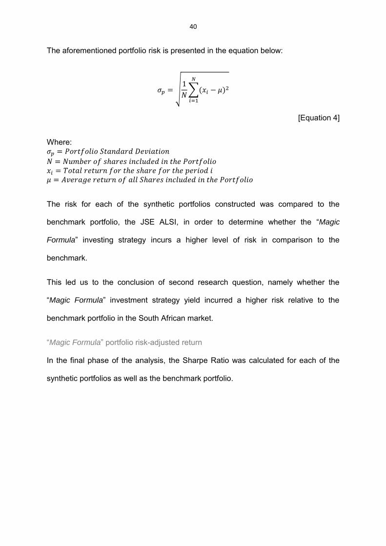
40
The aforementioned portfolio risk is presented in the equation below:
√
∑( )
[Equation 4]
Where:
The risk for each of the synthetic portfolios constructed was compared to the
benchmark portfolio, the JSE ALSI, in order to determine whether the “Magic
Formula” investing strategy incurs a higher level of risk in comparison to the
benchmark.
This led us to the conclusion of second research question, namely whether the
“Magic Formula” investment strategy yield incurred a higher risk relative to the
benchmark portfolio in the South African market.
“Magic Formula” portfolio risk-adjusted return
In the final phase of the analysis, the Sharpe Ratio was calculated for each of the
synthetic portfolios as well as the benchmark portfolio.

41
The Sharpe ratio (Sharpe, 1994) was calculated as follows:
[Equation 5]
Where:
The Sharpe ratio calculation is used as a measure of risk adjusted return and
enables us to conclude whether any of the synthetic “Magic Formula” portfolios
outperform the benchmark portfolio, the JSE ALSI, on a risk adjusted basis. This led
us to the conclusion of a third and final research question, namely whether the
“Magic Formula” investment strategy yielded a higher risk-adjusted return relative to
the benchmark portfolio in the South African market.
Strategic Considerations
In order to adequately address the 3 research questions, by performing the “Magic
Formula” analysis in accordance with the research design, additional factors needed
to be considered. These additional factors are highlighted in this section of the study
and include:
1. A consideration of the liquidity constraint, whereby the determination and
justification for companies to be included in the study from a liquidity
perspective is provided.
2. A consideration of the availability of information, whereby the
determination of what publicly available financial information would have

42
been available at the time of performing the calculation of the EY and ROC
ratios.
3. A consideration of data accuracy, whereby the determination,
documentation and adjustments of potential data outliers has been
addressed.
4. A consideration of the risk free rate, whereby the determination and
justification for the most appropriate risk free rate for the use in Equation
5 is provided.
1. Liquidity Constraint
Liquidity is generally viewed as the ability to trade large quantities quickly at low cost
with little price impact (Liu, 2006). Accordingly, liquidity is an important consideration
in the construction of any portfolio as the ability to realise a certain return, when
required, is imperative (Eltringham, 2014). This statement holds true to the
application of the “Magic Formula” and accordingly a liquidity element was
incorporated into this study, the details of which are provided below:
Minimum Market Capitalisation
Olin (2011), in the analysis of the “Magic Formula” on the Finnish Stock Exchange,
accounted for the liquidity risk by excluding all shares listed on the exchange which
reported a market capitalisation of less than £10 million from the portfolio
determination.
The analysis of various investing strategies on the JSE however has shown differing
approaches with regards to the population size.
Howard (2015) considered only the top 160 companies on the JSE. The same holds
true for Muller and Ward (2013) in their analysis of style-based effects on the JSE.
43
Van Rensburg and Robertson (2003) differed when performing their analysis of
cross section returns, as they only included the highest 100 shares by market
capitalisation. Contrastingly to the aforementioned studies, Hoffman (2012) included
the entire JSE in his analysis of share return anomalies.
As a result of these differences, there appeared to be no concrete solution to the
most appropriate population size to use in the analysis of the “Magic Formula” for the
South African market. Accordingly, it was undertaken to construct the synthetic
“Magic Formula” portfolios based on a population size which was greater than a
certain threshold, being a market capitalisation of R100 million, as opposed to a
certain fixed number of shares. This treatment coincides with that of Olin (2011) in
the application of the “Magic Formula” to the Finnish Market.
JSE ALTx
An additional consideration related to liquidity was whether or not to include the JSE
Alternative exchange (‘AltX’) into the “Magic Formula” analysis.
In order to address this question, a comparison, with particular emphasis on the
liquidity, between the JSE and JSE AltX was performed. Through this comparison it
was established that merely due to the differences in listing requirements (between
the JSE and the JSE AltX) it would imply that the risk of purchasing shares in the
AltX companies are slightly higher than on the JSE, simply because they (the
shares) may be harder to liquidate (Van Heerden, 2015).
Further to the above, the listing requirements of the JSE AltX also do not require a
profit history to be provided (Business Blue-Book of South African, 2008:6). The
implication of this is that by including companies which do not display a ‘proven track

44
record’ it could distort the underlying “Magic Formula” analysis as these companies
would ordinarily be weaned out by traditional market listing requirements.
As a result of the aforementioned factors, the JSE AltX was excluded from the scope
for this study.
2. Data Availability and Selection
In order to be sure of the “Magic Formula” investment strategy one must be certain
that the information was available at the time that the investment decision was made
(Olin, 2011).
In light of the above statement, in order to ensure that the information for the
calculation of the ROC and EY ratios was available at the time that the investment
decision was made, a fixed rebalancing date was set out in this analysis.
- Six month “Magic Formula” portfolios were rebalanced semi-annually on 1
April and 1 October each year.
- One year, two year and five year “Magic Formula” portfolios were rebalanced
on 1 October as required.
For each of the companies included in the dataset, using their respective financial
year end dates, it was determined whether interim financial results or year-end
financial results would be publicly available as at the applicable rebalancing dates (1
April or 1 October).
The determination of which company financial information would be available (i.e.
interim-year or final-year) was made based on the assumption that the release of
financial results trails the financial year-end and financial interim-end dates by three
months (KPMG, 2013). This assumption is supported by the JSE listing

45
requirements, whereby the provisional report or interim report must be made
available to the public at a minimum of three months after the respective interim-year
or final-year close (KPMG, 2013). Hence, the required information to calculate ROC
and EY would have been available for a particular share a minimum of three months
after the reporting date.
The details of the financial year-end dates and the applicable information assumed
to be available for the purposes of this study, in which to compute the ROC and EY
ratios, is provided in Table 4:
Table 4 - Publicly available information to compute ROC and EY ratios
Annual Financial Statement Dates
Year-end Date Information available
at 1 April Information available
at 1 October
January Interim Final February Interim Final
March Interim Final April Interim Final May Interim Final June Interim Final July Final Interim
August Final Interim September Final Interim
October Final Interim November Final Interim December Final Interim
Data Availability – Illustrative Examples
In order to explain Table 4 above, two illustrative examples have been included
below:
1. For the purposes of this illustrative example, assume the theoretical company
has a 30 June financial year end:

46
At the rebalancing date of 1 October, three months would have passed
since financial year end (July, August and September) and, as a result
of the JSE listing requirements, the latest final year financial results
would be publicly available.
Accordingly, the calculation of the EY and ROC ratios would be based
on this information as stated in the table above.
2. Assuming the theoretical company has a 31 July financial year end:
At the rebalancing date of 1 October, only two months would have
passed since financial year end (August and September) and as a
result the final year financial results would not yet be available for the
purposes of calculating the EY and ROC ratios.
Accordingly, the latest publicly available financial information, for use
as inputs in the EY and ROC calculations, would have been the
interim-year end results which would have been published three
months after the interim-year end of 31 January (31 January being six
months after financial year end).
It is noted that the interim financial information was used in the “Magic Formula”
analysis as it would represent the latest available financial information at the time of
the rebalancing date. Further, in order to ensure comparability to an annualised
figure, all income statement metrics at interim reporting were annualised prior to the
calculation of the ROC ratio.

47
3. Data accuracy – a reasonability check
In order to ensure the validity and accurateness of the results in this study, when
calculating the returns generated from the respective shares selected under the
synthetic “Magic Formula” portfolios, reasonability checks were performed on all
statistical outliers13 as determined using the Tukey (1997) methodology as described
below.
Statistical Outlier Determination
In determining what constituted a statistical outlier, the John Tukey outlier filter
(Tukey, 1977:43-44) was used as the quantitative basis. Importantly, for the
computation thereof, the JSE ALSI was used as a proxy as it represented the
benchmark portfolio (this is discussed in greater detail in the ‘Selecting the
Benchmark Portfolio’ section below).
Accordingly, by following the Tukey outlier filter methodology the annual JSE ALSI
returns were used to determine the 1st and 3rd quartiles as well as to calculate the
interquartile range as shown in Table 5 below:
13
Please refer to Definitions of Key Terms, Concepts and Variables in the Glossary for more information on statistical outliers.

48
Table 5 – Determination of what constitutes a statistical outlier
OBSERVATION JSE ALSI RETURN
10 37% 9 36% 8 27% 7 24% 6 21% 5 15% 4 8% 3 5% 2 4% 1 -18%
3rd Quartile (Q3) 26% 1st Quartile (Q1) 4%
Interquartile Range (IQR) 22% (Q3 - Q1)
1.5 x IQR 32%
Upper Outlier Determination 58%
(Q3 + 1.5 x IQR)
Lower Outlier Determination -28%
(Q1 - 1.5 x IQR)
As shown in table 5 above, in accordance with the Tukey outlier filter methodology
(Tukey, 1977:43-44), upper outliers were determined to be where the return
generated was greater 58%. This upper outlier determination was calculated as the
sum of the 3rd quartile return and 1.5 times the ‘interquartile range’14. Similarly, the
lower outliers were determined to be where the return was less than -28% which was
calculated as the 1st quartile less 1.5 times the interquartile range.
14
The Interquartile range, as shown in Table 5, refers to the difference between the 3rd and 1st quartiles (Tukey, 1977:43-44).

49
Reasonability Check Performed
The reasonability check performed on all statistical outliers, included, but was not
limited to:
- Verifying the inputs used to calculate the share return by agreeing the
respective share purchase and sale price information, as obtained from
Bloomberg, to a secondary source, namely McGregor BFA.
- Reviewing the SENS announcements of the company for the particular period
in question to identify any significant events, for which adjustments must be
made, such as share splits.
Adjustments made as a result of Reasonability Check performed on Identified
Outliers
Of the various outliers investigated as part of the reasonability check in this study,
only two differences requiring adjustment were encountered.
These two outliers were adjusted for accordingly, details of which are provided
below:
1. Combined Motor Holdings was selected in the 2006 rebalance date. The initial
analysis, as summarised in Figure 1 below, indicated a return on this share of
-82% thus triggering a statistical outlier.
Investigation into this outlier identified that, as shown in Appendix 2, the
reason for the decline was due to a share split. This was adjusted for by
multiplying the number of shares purchased, under the terms of the “Magic
Formula” by the share split ratio of 1:5.

50
Figure 1 – Combined Motor Holdings statistical outlier key information
Period 2006
TICKER
Share Price Bought
Share Price Sold % Change
CMH 94 16.5 -82% Investigate
Market Cap 1,990,995,200 McGregor BFA
Adjustment Number of Shares purchased x5
2. Assore Limited was selected in the 2009 rebalance date. The initial analysis,
as summarised in Figure 2 below, indicated a return on this share of -75%
thus triggering a statistical outlier.
Investigation into this outlier identified that, as shown in Appendix 3, the
reason for the decline was due to a share split. This was adjusted for by
multiplying the number of shares purchased, under the terms of the “Magic
Formula” by the share split ratio of 1:5.
Figure 2 – ASR statistical outlier key information
Period 2009
TICKER
Share Price Bought
Share Price Sold % Change
CMH 629.99 157 -75% Investigate
Market Cap 17,370,141,390 McGregor BFA
Adjustment Number of Shares purchased x5

51
4. Risk-Free Rate15
As established in the Sharpe Ratio formula set out in Equation 5, in order to
calculate the Sharpe Ratio, a risk-free rate was required to be determined. For the
purposes of this determination, bond yields are frequently used as the proxy for risk
free rates (EY, 2014). Accordingly, in determining an appropriate proxy in which to
measure the South African risk-free rate, details of the South African government
bonds were reviewed.
Based on the review performed, the long term government R186 bond was chosen
as the proxy for the risk free rate. The reason for choosing this long term government
bond was due to the following reasons:
i. The R186 becomes redeemable between 2025 and 2027 representing a long
term investment horizon. As the coupon rate of the R186 government bond
reflecting 10.5% does not change between the inception, being 1998, and
redemption dates, the yield thereon would represent an accurate reflection of
the long term interest free-rate.
ii. The bond covered the scope of the analysis. An alternative to the R186
government bond was the R157 government bond as used by Howard (2015)
in the comparable study. However, with the R157 maturing on 15 September
2014, this did not cover the entire investment period analysed in this analysis
and accordingly could not be used as a suitable proxy.
15
Please refer to Definitions of Key Terms, Concepts and Variables in the Glossary for more information on the Risk-Free rate concept.

52
Selecting the ‘Benchmark Portfolio’
As highlighted by Kruger and Van Rensburg (2008), benchmarks form an integral
component of fund management, both for active management who seek an
appropriate index against which to evaluate their performance as well as passive
management who seek an index to track.
The objective of the benchmark in this study is to serve as a proxy for the market. As
a result, the starting point was the JSE ALSI. This was due to the JSE ALSI
incorporating the top 99% of eligible listed companies ranked by full market
capitalisation (Grayswan, 2013) thus representing the majority of the market.
In assessing the appropriateness of this index as a viable benchmark, the traditional
inherent limitations of the ALSI, being the high levels of market concentration in
terms of market capitalisation and liquidity as well as a volatile resources sector
(Kruger and Van Rensburg, 2008), were considered. It was assumed that these
limitations all presented underlying market risks which would have been faced by an
investor when investing in the broad based South Africa market. As such, it was
concluded that these factors did not result in the JSE ALSI being excluded as a
viable proxy for the market.
Over and above the widespread representation of the market which the ALSI
provides, a further factor weighted in favour of selecting this index as the benchmark
portfolio is that it ensured comparability with the benchmark used by Howard (2015).
As a result of this it was concluded that the JSE ALSI was most appropriate
benchmark for the purposes of this study as it enabled comparability between the
two studies.

53
However, with the above being noted, it is understood that the JSE ALSI would
present specific limitations of the study. These limitations, impacting the
comparability between the “Magic Formula” return and the ‘market’ return, include:
1. The JSE ALSI is a market weighted index, whereas the “Magic Formula”
analysis constructs an equally weighted index.
2. The JSE ALSI includes financial services firms within the index, contrastingly
all financial services companies are excluded from the “Magic Formula”.
Validated Data Sources
Sources of Quantitative Data
In performing the quantitative aspects of the “Magic Formula” analysis, the data was
obtained from a variety of sources and exported into excel for further analysis.
Details of the sources used in the analysis, as well as the reasoning thereof, are as
follows:
The company financial statements data16 was sourced from S&P Capital IQ. S&P
Capital IQ was chosen for this component of the data gathering phase as it returned
specified data for certain shares, i.e. those shares included in the scope of analysis,
for an extended period of time in an easily usable format.
The market capitalisation and share price data, as at the 1 October and 1 April
dates, was sourced from a Bloomberg terminal. Bloomberg was chosen for this
aspect of the data gathering phase as it provided accurate, historical, market
information for the entire JSE.
16 The Company financial statements data refers to the information which appears on the annual financial statements. Of the inputs required for the “Magic Formula” analysis it includes: EBIT, Total Assets, Total Liabilities, Current Assets, Current Liabilities, Cash & Cash Equivalents, Goodwill and DPS.

54
The benchmark, the JSE ALSI (J203), as well as the share price data for the
validation checks was sourced from McGregor BFA. This platform was used for this
section of the data gathering phase as it provided specific detail required from the
benchmark, namely the price data and annualised volatility, as well as providing an
appropriate secondary source in which to verify certain share price information
obtained from the Bloomberg terminal above.
Validating Quantitative Data Gathered
The effectiveness of any study is only as accurate as the information used in
performing the analysis. Accordingly, all the data was sourced from reputable
companies which specialise in providing financial information. It must be noted
however, that while using reputable sources such as S&P Capital IQ, Bloomberg and
McGregor BFA minimises the risk of data inaccuracy, there still exists the possibility
of certain data imperfections.
As a result, in order to limit the impact of potential data imperfections in the study,
certain data validation checks were put into place when constructing the financial
model. These validation checks are described briefly below:
- Should information, relevant for the purposes of calculating the ROC or EY
ratios be missing then a 0% ratio was returned resulting in the specific
company being excluded from the lowest combined rankings selection criteria.
Accordingly, this resulted in the specific company being excluded from the
analysis at the specific rebalance date for which information was missing.
- As described under the Strategic Considerations section, certain validation
checks were also performed on results where statistical outliers were noted.
Where adjustments were required to accurately reflect the substance of the
55
company return, they were made accordingly using the results obtained from
alternative data sources.
As an additional data reliability test, the market data used in performing the statistical
analysis was used to re-calculate the return of the JSE ALSI. The result of which, as
shown in Figure 3, was plotted against the actual return of the JSE ALSI for
comparison.
In completing this reconstruction of the JSE ALSI and determining the total returns
generated from the index the below formulas, as obtained from the FTSE/JSE
(2004), were used:
∑( )
[Equation 6]
Where:
In determining the Index value above, for the purposes of the recalculation, the top
165 shares were included into the reconstructed index with the following treatment
being applied:
- The exchange rate (e) was not applicable as all figures, in the data which was
collected, were denominated in South Africa Rands (ZAR). Accordingly, a
factor of 1 was used for this input in the calculation.

56
- The resultant share price (p) multiplied by the number of shares (s) would
equate to the market capitalisation. As a result, the market capitalisation
figure was used to represent this portion of the computation.
- A free float factor (f) of 1 was used in the calculation as it represented an
assumption that all shares in the index were tradable (FTSE/JSE, 2014:11).
This is consistent with the treatment applied when conducting the study.
- The divisor (d) is included in the index calculation, as shown in equation 6
above, to account for rights issues initiated during the period. By including the
divisor into the calculation it ensures that the index falls in line with the
reduction in share price on the right ex-date (FTSE/JSE, 2014:19).
With this being the case, in order to simplify the reconstruction, no divisor was
used in the reconstruction performed in this study. This may result in certain
differences between the reconstructed and the actual JSE ALSI however, as
the purpose of this is merely to provide a reasonability test, the potential
differences are accepted.
Having calculated the index value, the returns of the reconstructed index were
required to be compared to the returns generated from the actual JSE ALSI.
Accordingly, the total returns were calculated in accordance with the following
formula as outlined in FTSE/JSE (2004):
[Equation 7]
Where:
( ) ( )

57
( ) ( )
It must be noted, that for the purposes of calculating the Total Returns Index for
comparison, the only adjustment which was applied to the capital index was that of
the dividends earned by all the companies included in the listing.
Figure 3 – Reconstructed ALSI using annual market data gathered for statistical
analysis
As can be seen from Figure 3 above, the theoretic return generated from the
reconstructed market data approximates that of the JSE ALSI and as a result it
would indicate that the information used for the purposes of performing the analysis
is accurate.
-30%-20%-10%
0%10%20%30%40%50%
01-S
ep-0
601
-May
-07
01-J
an-0
801
-Sep
-08
01-M
ay-0
901
-Jan
-10
01-S
ep-1
001
-May
-11
01-J
an-1
201
-Sep
-12
01-M
ay-1
301
-Jan
-14
01-S
ep-1
401
-May
-15
No
rmalised
Cu
mla
tiv
e R
etu
rns
Market Data comparison to JSE ALSI
RECALCULATED TRI
ALSI TRI

58
Ethical Considerations
No ethical clearances were required for any component of this study as no interest in
gender nor racial differences and no participation human participants was necessary
for the completion of this research.
In relation to the confidentiality of information used, all of the information which was
obtained is publicly and readily available from the sources as highlighted above.
Limitations of the Study
In determining the optimal “Magic Formula” portfolio, transaction costs and taxes
were excluded from the analysis. This treatment was consistent with the work
performed in alternative studies by Howard (2015), Hoffman (2012) and Muller and
Ward (2013) on the basis that these costs would not differ significantly amongst
portfolios and as a result they are immaterial to the investment decision.
In respect of the portfolio construction, the ‘five year’ portfolio only results in two
observable periods. Accordingly, the limited number of observations may impact on
the ability to draw accurate and meaningful conclusions in relation to this portfolio
holding period.
Lastly, in relation to the measurement of risk, the volatility of portfolio returns has
been used as a proxy. As a result, the study, relies on a normal distribution of returns
to evaluate risk for a value investing metric which assumes that market efficiency
does not apply.

59
CHAPTER 4 - RESULTS
This chapter presents the findings of using the “Magic Formula” investment strategy
in the South African market for various portfolio sizes and holding periods. The
returns generated, risk incurred and risk adjusted returns manufactured from the
synthetic portfolios which were created will be compared to the JSE ALSI as well as
to each other in order to address the three primary research questions.
The results for each of the three primary research questions, as set out on page 29,
will be addressed independently and sequentially throughout this section and in
addressing the results for each of the three research questions, the results will be
presented followed by a discussion thereof.
Performance of “Magic Formula” investment strategy
The first section of the results chapter will cover the first two research questions by
determining and discussing the returns generated as well as the risk incurred from
the “Magic Formula” investment strategy.
In addressing the “Magic Formula” portfolio return, the ‘portfolio size’ and ‘portfolio
holding period’ shall first be discussed independently followed by a discussion on
which combination of these two portfolio structure constituents yields the highest
return for the “Magic Formula” in the South African market. This will lead us to the
conclusion of the first research question.
Subsequently to addressing the first research question, the two additional research
questions (research questions 1(i) and 1(ii)) which will provide substantiation to the
results shown for research question one shall be discussed.

60
The final component to be addressed in this section of the chapter is the “Magic
Formula” portfolio risk. Similarly to the manner in which the portfolio return was
presented, the “Magic Formula” portfolio risk shall address first the ‘portfolio size’
and ‘portfolio holding periods’ followed by which combinations of these two portfolio
structure constituents results in the highest “Magic Formula” portfolio risk being
incurred. This will lead us to the conclusion of the second research question.
“Magic Formula” Portfolio Return
The synthetic “Magic Formula” portfolios, which vary the holding period and number
of shares, created by selecting the best shares based on a combined ranking of
ROC and EY prove to be highly successful in the South African market. As shown in
Figure 4, the majority of these constructed portfolios yielded a greater geometric
mean return than the benchmark with only the five year – 5, 10, 15 & 20 share and
the two year – 5 share combinations underperforming the JSE ALSI. A summary of
these results, presented numerically, is provided in Appendix 1.
Figure 4 – Portfolio Geometric Mean Returns
5% 7%
10%
13%
0%
5%
10%
15%
20%
25%
5 Shares 10 Shares 15 Shares 20 Shares
An
nu
alised
av
era
ge R
etu
rn (
%)
Mean Portfolio Returns
Six month
One year
Two year
Five year
JSE ALSI

61
Portfolio Size
When looking at the performance of the different portfolios from a number of shares
to be included in the portfolio perspective, it can be seen in Figure 4 above that each
of the respective rebalance frequencies (with the exception of the 5 year portfolio)
has a trend of an increasing mean return as the number of shares included in the
portfolio increases. This trend exists up to a “breaking point” at which time the mean
return of the portfolio starts to diminish.
Table 6 – Breaking point of number of shares to be included in the “Magic Formula”
portfolio
BREAKING POINT
SIX MONTH 15 Shares ONE YEAR 10 Shares TWO YEAR 15 Shares FIVE YEAR N/A
The implication of a breaking point being observed in these portfolios (i.e. 10 and 15
shares) has a twofold application:
Firstly, the breaking point of a one year portfolio, being 10 shares, indicates that the
use of 30 shares by Howard (2015) in prior research performed on the “Magic
Formula” did not optimise the mean return from the investment strategy. This was
corroborated through the reconstruction of a one year – 30 shares portfolio in which
it was found that a mean return of 19% was generated (Appendix 1).
The mean return of 17% generated from the one year – 30 share portfolio falls below
the mean return of 18% generated from the one year – 20 share portfolio. This would

62
indicate that once the breaking point is surpassed, each share added to the portfolio
would bring about a marginal decrease in the total mean return.
Secondly, the breaking point of six month, one and two year portfolios suggest that
the optimal number of shares, from a mean return generating perspective falls
between these two portfolio sizes. This is corroborated by Table 7 which, once
removing the five year portfolio, indicates that portfolio sizes of between 10 and 20
shares offer similar returns and similar rates of outperformance on a geometric mean
return basis.
Table 7 – Average Geometric returns generated from the various portfolio sizes
5
SHARES 10
SHARES 15
SHARES 20
SHARES AVERAGE GEOMETRIC RETURN 15.19% 18.82% 19.40% 18.23%
In relation to the five year portfolio, it is important to note that the potential reason for
this portfolio not incurring a breaking point, as shown by the other portfolios, may be
as a direct result of only being exposed to two rebalancing periods (1 October 2005
and 1 October 2010) thus potentially skewing the results contained therein.
Holding Period
When looking at the holding period impact on the overall return, as shown in Figure
4 above and Table 8 below, it indicates that the optimal holding period lies between
‘six months’ and ‘one year’ as these holding periods generate the highest mean
returns and are the least sensitive to change in the number of shares making up the
portfolio.

63
The five year portfolios are found to have the lowest geometric mean returns. This
would indicate that fewer ‘winners’ are picked as a result of the less frequent
rebalancing resulting in diminishing returns for “Magic Formula” portfolios which have
a holding period of greater than two years. Further implication of this result is that the
five year portfolio also contrasts to the fundamental principle of value investing which
prescribes that value investing stocks should always ‘win’ over longer holding
periods (Novy-Marx, 2013).
Table 8 – Average returns generated from the various holding periods
SIX MONTHS
ONE YEAR
TWO YEAR
FIVE YEAR
AVERAGE GEOMETRIC RETURN 18.26% 18.28% 17.18% 8.96%
SENSITIVITY OF RETURNS TO A CHANGE IN NUMBER OF SHARES WITHIN PORTFOLIO
7.95% 8.56% 14.23% 34.64%
When looking at the geometric mean return in isolation, it would suggest,
contrastingly to the portfolio size, that the one year holding period recommendation
by Greenblatt (2006) and subsequently applied by Howard (2015) in his application
of the “Magic Formula” to the South African market would result in the highest
geometric return.
However, in relation to the holding period, the one year portfolio yields the highest
mean return yet suffers from a higher standard deviation of returns in comparison to
the six month and two year portfolios. This implies that on a risk adjusted basis we
cannot determine, without additional analysis, whether the outperformance
generated by the one year portfolio is as a result of superior performance of the
underlying investment strategy or as a result of additional risk exposure to which the
one year portfolios are exposed. More detail and analysis, relating to the risk

64
adjusted return, is provided in the ‘Risk-adjusted returns of the “Magic Formula”
portfolio’ section to follow.
In relation to the sensitivity shown in Table 8, the portfolio least sensitive to the
number of shares included within it relates to the six month portfolio, in other words
the period with the most frequent rebalancing. This may indicate that by perusing a
six month “Magic Formula” holding period you are taking advantage of a short term
mispricing in the market as identified by the ROC and EY ratios resulting in “smaller”
less volatile gains.
Optimal mean-return generating combination of Portfolio size and Holding Period
Based on the isolated discussions regarding the portfolio size and holding period
above, the top three mean generating “Magic Formula” portfolios all consist of
various derivations of the optimal constituents. A summary of Appendix 1,
displaying the values of the top three mean return synthetic portfolios, is provided in
Table 9 below.

65
Table 9 – Highest mean return generating “Magic Formula” portfolios
SIX
MONTH ONE
YEAR TWO YEAR
TOTAL RETURN 15
SHARES 10
SHARES 15
SHARES 2005 to 2006 35% 36% 161% 2006 to 2007 78% 52% 2007 to 2008 -21% -26%
-13% 2008 to 2009 13% 9% 2009 to 2010 10% 10%
28% 2010 to 2011 14% 4% 2011 to 2012 38% 48%
62% 2012 to 2013 32% 45% 2013 to 2014 17% 30%
30% 2014 to 2015 6% 19%
ANNUALISED GEOMETRIC
MEAN 19.8% 20.3% 19.8%
Initial Portfolio Value 1 000 1 000 1 000
Ending Portfolio Value 6 106 6 374 6 099
Compound Annual Growth
Rate 19.8% 20.3% 19.8%
As shown in Table 9, the “Magic Formula” investment strategy does beat the market
on an annualised mean return basis with the top three portfolio size and holding
period combinations of one year – 10 shares, six month – 15 shares, and two years
– 15 shares yielding a Compound annual growth rate (‘CAGR’) of 20.3%, 19.8% and
19.8% respectively. Comparatively, the JSE ALSI17 showed a CAGR of 14.8% for
the same period, thus resulting in an outperformance of 5.5%, 5.0% and 5.0% for the
same aforementioned portfolios over the 10 year period.
17
For a graphical representation of the cumulative performance of the “Magic Formula” against the
JSE ALSI please refer to Appendix 12.

66
Importantly, the investment strategy does not only beat the benchmark portfolio, on a
pure mean return basis, for the constructed portfolios shown in Table 9 above but
also for 8 of the remaining 13 synthetic “Magic Formula” portfolios created.
Conclusion on Research Question 1
As a result of the above discussion, along with the returns shown in appendix 1, it is
concluded, consistently with the findings from Howard (2015), that the “Magic
Formula” investment yields superior returns relative to the benchmark portfolio in the
South African market.
“Magic Formula” investment strategy impact on returns
Introduction
Having determined that the returns generated by the “Magic Formula” investment
strategy outperforms the benchmark portfolio, it would lead us to the consideration
and execution of research question 1(i), as outlined under Chapter 3 of this study.
Accordingly, in this section it shall be determined whether the returns generated by
the “Magic Formula” investment strategy were random through the construction of
the inverse “Magic Formula” investment portfolios.
Results and Discussion
The results of the inverse portfolios, as shown in Table 10, all differ from the
traditional “Magic Formula” portfolios. This would indicate that the returns generated
by the “Magic Formula” investment strategy are not generated randomly and that
there is a causal relationship between the “Magic Formula” investment basis and the
returns generated.

67
Table 10 – Inverse “Magic Formula” portfolios
1 YEAR 2 YEAR
TOTAL RETURN 10
SHARES 10
SHARES 15
SHARES 2005 to 2006 39% 75% 86% 2006 to 2007 47% 2007 to 2008 -34% -41% -17% 2008 to 2009 -28% 2009 to 2010 -14% -14% 14% 2010 to 2011 -32% 2011 to 2012 -5% 25% 47% 2012 to 2013 20% 2013 to 2014 -6% -33% -14% 2014 to 2015 -16% Annualised
Average -3% 1% 12%
Initial Portfolio Value 1 000 1 000 1 000
Ending Portfolio Value
514
752 2 217
CAGR -6% -3% 8%
In order to support the conclusion made above, which indicates that the returns
generated by the “Magic Formula” portfolio are not random and that the “Magic
Formula” selection basis influences the returns generated, a paired t-Test was
performed over representative portfolios. Performing this t-Test allows us to
determine whether the differences in the mean return, noted between Table 9 and
10, are statistically significant.
Should the null hypothesis, presented in Equation 8 below, not be rejected in the t-
Test analysis then it is concluded that the differences observed between the “Magic

68
Formula” and the inverse thereof are not statistically significant. Accordingly, this
would indicate that returns generated are random from a statistical perspective.
The t-Test was constructed using the annual mean returns generated from the
respective portfolios with the significance level being set at 95%.
H0: µ“Magic Formula” P f = µI v “Magic Formula” P f
[Equation 8]
Where:
The portfolios used to perform this t-Test were the one year – 10 shares “Magic
Formula” portfolio and its inverse counterpart. It is noted that the one year portfolios
were selected for ease of computation as all the information contained therein was
already annualised allowing for accurate comparison.
Figure 5 – t-Test results of “Magic Formula” influencing portfolio returns
t-Test: Paired Two Sample for Means
"Magic Formula"
Inverse "Magic Formula"
Arithmetic mean 0.227 -0.028 Variance 0.060 0.084 Observations 10 10 Pearson Correlation 0.800 Hypothesized Mean Difference 0.000 Df 9.000 t Stat 4.635 P(T<=t) one-tail 0.001 t Critical one-tail 1.833 P(T<=t) two-tail 0.001 t Critical two-tail 2.262

69
As the paired t-Test result indicates a P(T<=t) two-tail, which represents the p value,
value of 0.001 which is lower than the significance level of 0.05 it would lead us to
reject the null hypothesis.
Conclusion on Research Question 1(i)
As the null hypothesis, as shown by Equation 8 above, is rejected it would lead us
to conclude, on a statistically significant basis, that the “Magic Formula” selection
basis influences the returns. Accordingly, this leads to the conclusion of research
question 1(i) whereby it is determined that the returns generated by “Magic Formula”
investment strategy are not random.
Comparison to alternative study
Introduction
The 20.3% return generated from the top performing “Magic Formula” portfolio, on a
geometric mean basis as shown in Table 9, differing from the 18.75% return shown
by Howard (2015) in the alternative study conducted over the “Magic Formula” in the
South African market begs the question of whether the studies are comparable.
Answering the above question, as represented by additional research question 1(ii),
is of high importance because should the studies not be comparable and it is found
that “Magic Formula” outperforms the benchmark then we will be unable to conclude
that this outperformance is due to altering the portfolio size and holding period as the
outperformance may relate to the differences in periods over which the “Magic
Formula” is applied.

70
Results and Discussion
In accordance with Chapter 3, an additional synthetic portfolio (Portfolio 17), using
the dataset of this study, was created under the terms set out by Howard (2015).
This portfolio reflected a one year holding period with a portfolio size of 30 shares.
Table 11 – Comparison to “Magic Formula” to alternative study
1 YEAR 30 SHARES
TOTAL RETURN
Howard (2015)
Ker-Fox (2017)
2005 to 2006 48% 33% 2006 to 2007 25% 46% 2007 to 2008 -20% -24% 2008 to 2009 34% 3% 2009 to 2010 30% 19% 2010 to 2011 4% 19% 2011 to 2012 23% 41% 2012 to 2013 10% 28%
Geometric Mean 17.52% 18.38%
Refer to Appendix 4 for a full listing of the results recorded by Howard (2015:38)
The comparison, as shown in Table 11, was generated for all years of overlap
between the two studies, namely 2005 to 2013, and resulted in a geometric mean
return difference of 1% being found.
The reason for the 1% geometric mean return difference being observed is believed
to be derived primarily from two key factors. These factors are discussed below:
The first factor which is believed to give rise to the differences observed, particularly
at a yearly breakdown, is the differing portfolio rebalancing dates. In the study
conducted by Howard (2015), the portfolio is stated to be rebalanced in December
annually. Comparatively, this study rebalances the portfolio annually in October. The

71
implication of this difference, as outlined in Chapter 3 – Strategic Considerations,
would be that different information would be publicly available in which to calculate
the ROC and EY ratios. This could result in there being a difference in the respective
portfolio compositions which would lead to the geometric mean return differences as
observed. Due to the nature of this factor, quantitatively measuring the difference
was impracticable without re-performing the entire study. As a result, the differences
caused by this factor were deemed to be un-adjustable and were accepted as being
reasonable for the purposes of the study.
The second factor is that certain adjustments for statistical outliers, as previously
discussed, were made in carrying out the execution of this study. As there was no
indication of adjustments being made in the comparable study, processing
adjustments for share splits, as performed above for JSE:CMH in 2006 and
JSE:ASR in 2010, would give rise to a measureable difference between this study
and that of the comparable study.
A comparison of the “Magic Formula” portfolio constructed in this study, whereby the
adjustments which were made in respect of share splits of the statistical outliers
have been removed, and that presented by Howard (2015) is shown in Table 12
below:
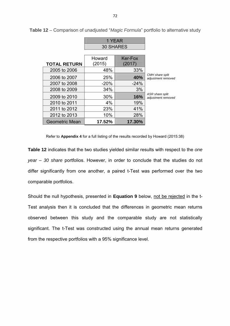
72
Table 12 – Comparison of unadjusted “Magic Formula” portfolio to alternative study
1 YEAR 30 SHARES
TOTAL RETURN
Howard (2015)
Ker-Fox (2017)
2005 to 2006 48% 33%
2006 to 2007 25% 40% CMH share split adjustment removed
2007 to 2008 -20% -24% 2008 to 2009 34% 3%
2009 to 2010 30% 16% ASR share split adjustment removed
2010 to 2011 4% 19% 2011 to 2012 23% 41% 2012 to 2013 10% 28%
Geometric Mean 17.52% 17.30%
Refer to Appendix 4 for a full listing of the results recorded by Howard (2015:38)
Table 12 indicates that the two studies yielded similar results with respect to the one
year – 30 share portfolios. However, in order to conclude that the studies do not
differ significantly from one another, a paired t-Test was performed over the two
comparable portfolios.
Should the null hypothesis, presented in Equation 9 below, not be rejected in the t-
Test analysis then it is concluded that the differences in geometric mean returns
observed between this study and the comparable study are not statistically
significant. The t-Test was constructed using the annual mean returns generated
from the respective portfolios with a 95% significance level.

73
H0: µKer-F x “Magic Formula” P f = µH w “Magic Formula” P f
[Equation 9]
Where:
The paired t-Test result, shown in Figure 6, indicates a P(T<=t) two-tail p-value of
0.997 which is higher than the significance level of 0.05. This would lead us to not
reject the null hypothesis and conclude, on a statistically significant basis, that the
“Magic Formula” portfolio constructed in this study and the “Magic Formula” portfolio
constructed by Howard (2015) do not differ significantly.
Figure 6 – t-Test results of South African “Magic Formula” portfolio comparisons
t-Test: Paired Two Sample for Means
Howard "Magic Formula" Portfolio
Ker-Fox "Magic Formula" Portfolio
Arithmetic mean 0.1929 0.1932 Variance 0.0438 0.0474 Observations 8 8 Pearson Correlation 0.603
Hypothesized Mean Difference 0 df 7 t Stat -0.004 P(T<=t) one-tail 0.498 t Critical one-tail 1.895 P(T<=t) two-tail 0.997 t Critical two-tail 2.365
Conclusion on Research Question 1(ii)
As a result of the t-Test shown in Figure 6 above, we have established that this study
is comparable to that presented by Howard (2015). The implication of this is that any

74
additional return generated by altering either the holding period or the portfolio size is
as a direct result of changing those variables and not due to differences in underlying
data.
Accordingly, finding the combination of portfolio size and holding period which yields
the greatest geometric mean return per given level of risk would present the optimal
“Magic Formula” in the South African market. Comparison of this portfolio to the
benchmark would enable us to conclude on whether the same findings of
outperformance as observed by Greenblatt (2006), for the US market, and Olin
(2011), for the Finnish market, hold for the South Africa.
“Magic Formula” Portfolio Risk
The volatility of returns, as measured by standard deviation, was carried out across
all synthetic portfolios constructed. The results, as shown in Appendix 5, are
summarised for analysis in Figure 7 below:
Figure 7 – Portfolio Standard Deviation of Returns
9% 10% 13% 11%
0%
5%
10%
15%
20%
25%
30%
35%
40%
5 Shares 10 Shares 15 Shares 20 Shares
An
nu
alised
Geo
metr
ic S
tan
dard
D
ev
iati
on
(%
)
Portfolio Risk
Six month
One year
Two year
Five year
JSE ALSI
75
Similar to the comparison performed between the geometric mean returns and JSE
ALSI, the synthetic portfolios yielded a higher variability of return in comparison to
the benchmark portfolio for ten of the sixteen portfolios constructed. This may
indicate that the additional return generated by the “Magic Formula” investment
strategy was only as a result of the increased risk to which the investor was
exposed.
At a high level, it is evident that the five year “Magic Formula” portfolios yield the
lowest variability in returns. This indicates that the “Magic Formula” may produce
lower, but more consistent returns over a longer investment horizon. This is an
important consideration when bearing in mind the investor risk profile as well as the
resultant overall risk adjusted return. These factors are discussed in further detail in
the ‘risk-adjusted returns of the “Magic Formula” portfolio’ section below.
Portfolio Size
As can be seen in Figure 7, all of the varying holding periods follow the same trend
when it comes to the portfolio size. This trend being that as the number of shares
increases to a peak portfolio size of 15 shares so too does the variability of returns.
Thereafter, as the portfolios size increases, the standard deviation (measuring the
variability of returns) starts to diminish. This trend is expected to continue until all
constituents of the JSE ALSI are represented in the portfolio at which point the JSE
ALSI annualised volatility of 19% should be achieved.

76
The aforementioned trend is displayed numerically in Table 13 below:
Table 13 – Average Standard deviation generated from the various portfolio sizes
5 SHARES 10 SHARES 15 SHARES 20 SHARES AVERAGE GEOMETRIC STD. DEVIATION
17.45% 20.86% 23.56% 22.26%
The impact of a change in portfolio size on the geometric standard deviation is
closely aligned to that observed with the geometric mean return. This observation, as
displayed in Figure 8 below, is supported by the high correlation between these two
trends. The implication of this observation is that any additional return generated, as
a result of an adjustment to the portfolio size, is a direct result of the increased risk to
which the investor is exposed. Accordingly, any adjustment made to the “Magic
Formula” portfolio size, in isolation, will not generate significant excess risk-adjusted
returns.

77
Figure 8 – Geometric mean and geometric Standard deviation portfolio size
correlation.
Correlation:
GEOMETRIC
MEAN RETURN GEPMETRIC STD
DEVIATION
GEOMETRIC MEAN RETURN 1 GEPMETRIC STD DEVIATION 0.93 1
A further observation which can be made from Figure 8 is that the margin between
the geometric mean return and the geometric standard deviation is at its minimum at
the 10 share portfolio size. This indicates that, on average, the 10 share portfolio
size would generate the lowest risk adjusted returns in comparison to the alternative
portfolio sizes in the study. This observation, and confirmation on whether or not it is
found to be true, shall be reviewed in greater detail in the section to follow.
In review of Table 13, while the 5 share portfolios displayed the lowest volatility, this
was also the only grouping where more than one holding period yielded a standard
0.00%
5.00%
10.00%
15.00%
20.00%
25.00%
5SHARES
10SHARES
15SHARES
20SHARES
Perc
en
tag
e
Portfolio Size correlation between Geometric Mean & Geometric
Standard Deviation
GEOMETRICMEAN RETURN
GEOMETRICSTANDARDDEVIATION
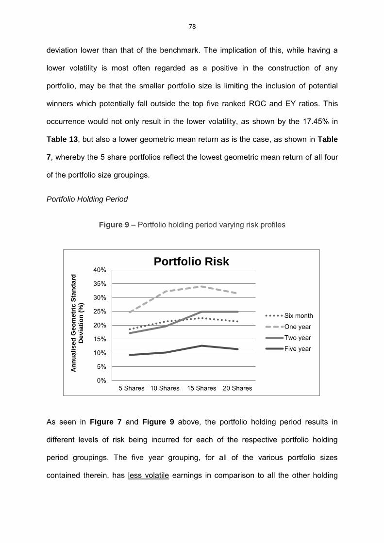
78
deviation lower than that of the benchmark. The implication of this, while having a
lower volatility is most often regarded as a positive in the construction of any
portfolio, may be that the smaller portfolio size is limiting the inclusion of potential
winners which potentially fall outside the top five ranked ROC and EY ratios. This
occurrence would not only result in the lower volatility, as shown by the 17.45% in
Table 13, but also a lower geometric mean return as is the case, as shown in Table
7, whereby the 5 share portfolios reflect the lowest geometric mean return of all four
of the portfolio size groupings.
Portfolio Holding Period
Figure 9 – Portfolio holding period varying risk profiles
As seen in Figure 7 and Figure 9 above, the portfolio holding period results in
different levels of risk being incurred for each of the respective portfolio holding
period groupings. The five year grouping, for all of the various portfolio sizes
contained therein, has less volatile earnings in comparison to all the other holding
0%
5%
10%
15%
20%
25%
30%
35%
40%
5 Shares 10 Shares 15 Shares 20 Shares
An
nu
alised
Geo
metr
ic S
tan
dard
D
ev
iati
on
(%
)
Portfolio Risk
Six month
One year
Two year
Five year

79
period groupings. On the other end of the spectrum, the entire one year portfolio, for
all of the various portfolio sizes contained therein, has more volatile earnings in
comparison to the other holding period groupings.
The only holding period groupings which result in a change in the level of risk as the
number of shares in the grouping increased is the six month and two year portfolios.
The overlap of these two groupings, indicating a change in the level of risk, occurs
approximately at a portfolio size of 12 shares. At this point of overlap, the risk of the
six month and two year portfolios are approximately the same. However, a portfolio
size smaller that 12 would indicate that the six month portfolio is exposed to a higher
volatility of returns whereas a portfolio size of more than 12 shares would indicate
that the two year portfolio is exposed to a higher volatility.
The aforementioned observation ties into the numerical representation provided in
Table 14 which shows the six month portfolios as being the least sensitive to a
change in the number of shares within the portfolio. Contrastingly, the two year
portfolios are the most sensitive to a change in the number of shares. The
differences in sensitivity, coupled with the similar overall geometric standard
deviation observed, result in the overlap between these two portfolio groupings being
observed as the number of shares included in the portfolio increases.

80
Table 14 – Average Standard Deviation generated from the various portfolio holding
periods
SIX MONTH
ONE YEAR
TWO YEAR
FIVE YEAR
AVERAGE GEOMETRIC STD DEVIATION
21.01% 30.63% 21.65% 10.85%
SENSITIVITY OF RETURNS TO A CHANGE IN NUMBER OF SHARES WITHIN PORTFOLIO
7.09% 11.45% 15.46% 11.74%
The advantage of being able to identify the level of risk incurred is valuable as this
can be used to tailor the best performing “Magic Formula” portfolios to specific
individual investor requirements. In other words, by being able to identify which
holding period results in the overall highest or lowest level of risk, a risk-averse
investor wishing to follow the “Magic Formula” would be able to construct the
portfolio which is found to outperform the market on a risk adjusted basis while
incurring the lowest level of risk, namely the five year portfolio.
Combination of Portfolio Size and Holding Period
In summary of the above, it was found that the portfolio holding period is a large
determinant in the level of risk faced by the “Magic Formula” portfolio with one year
portfolios yielding the highest variability of returns. Further, as presented by the small
differences in standard deviation observed between portfolio sizes of 10 to 20 years,
as shown in Table 13, along with the low sensitivity of portfolio returns to portfolio
size, as shown in Table 14, it can be confirmed that the portfolio size factor has little
impact on this risk.

81
As a result, due to one year portfolios yielding the highest variability of returns, the
portfolios which have the highest geometric standard deviation all consist of a one
year holding period.
A summary of Appendix 5, displaying the values of the top 3 portfolios generating
the highest variability of returns, is provided in Table 15.
Table 15 – Highest geometric average standard deviations “Magic Formula”
portfolios generated
ONE YEAR
10
SHARES 15
SHARES 20
SHARES 2005 to 2006 18% 40% 38% 2006 to 2007 36% 35% 32% 2007 to 2008 30% 25% 25% 2008 to 2009 26% 26% 25% 2009 to 2010 25% 29% 27% 2010 to 2011 25% 29% 27% 2011 to 2012 56% 51% 46% 2012 to 2013 29% 26% 24% 2013 to 2014 37% 44% 40% 2014 to 2015 44% 38% 35% GEOMETRIC AVERAGE
32.2% 34.0% 31.6%
After a review of all the synthetic “Magic Formula” portfolios variability of returns, it is
important to note, as eluded to in the discussion of the geometric mean returns, that
the one year holding period assumption applied by Howard (2015) in the application
of the “Magic Formula” to the South African market does not present the optimal
portfolio from a risk adjusted return perspective.
This statement is made as a result of, as shown and supported by the figures in
Table 16, the one year holding period marginally earning the highest geometric

82
mean return, however the risk incurred therein is significantly higher in comparison to
the next best geometric mean return generating portfolio grouping, the six month
portfolio.
Table 16 – One year vs six month holding periods impact on risk adjusted returns
SIX MONTHS ONE YEAR GEOMETRIC MEAN RETURN 18.26% 18.28%
GEOMETRIC STD DEVIATION 21.01% 30.63%
The assessment made above is further supported by the finding that, of the three
portfolios which generate the highest variability of returns as shown in Table 15, only
one, being the one year – 10 shares portfolio, is on the list of the top mean
generating portfolios as shown in Table 9. This would imply that the additional risk,
to which the one year portfolios are exposed, does not result in excess mean
generating returns being earned.
Conclusion on Research Question 2
As shown in Appendix 5 and discussed in detail in the section above, the majority of
the “Magic Formula” portfolios, with the majority being 11 of the 16 synthetically
constructed portfolios, incurred a higher level of risk in comparison to the benchmark
portfolio. Accordingly it is concluded that, on a pure volatility of returns basis, the
“Magic Formula” investment strategy is exposed to a higher level of risk relative to
the benchmark portfolio in the South African market.
83
Risk-adjusted returns of the “Magic Formula” portfolio
The results of the initial research questions, which found that both the “Magic
Formula” geometric mean return as well as the “Magic Formula” standard deviation
of returns exceeded the benchmark portfolio, leads us directly to research question
3. Accordingly, the determination and discussion of whether the “Magic Formula”
investment strategy outperforms the benchmark, as represented by the JSE ALSI,
on a risk adjusted basis shall be included in this section of the study.
This segment of the results chapter will be outlined as follows:
In the first subsection, the portfolio returns, for each of the synthetic portfolios
created (i.e. Portfolio 1 to Portfolio 17), shall be reviewed with reference to the risk
incurred for each of those respective portfolios.
Subsequently, in accordance with the research design set out in chapter 3 above,
the Sharpe ratio for each of the synthetic portfolios shall be calculated. This shall be
performed in order to quantify the risk-adjusted returns and determine whether any
of the synthetic “Magic Formula” portfolios outperform the benchmark portfolio, as
represented by the JSE ALSI.
Based on the results of the Sharpe ratio, a discussion surrounding the ‘optimal’
“Magic Formula” portfolio in the South African market shall be provided. In
addressing the question of: ‘What is the optimal “Magic Formula” portfolio for the
South African market?’ the risk tolerance of investors shall be taken into account and
shall form the basis of the discussion.
Lastly, it shall be determined whether the outperformance of the “Magic Formula”
risk-adjusted returns relative to the JSE ALSI, if any, is statistically significant. This

84
will lead us to the conclusion of research question 3, namely: ‘Does the “Magic
Formula” investment strategy outperform the benchmark portfolio on a risk-adjusted
basis in the South African market?
“Magic Formula” Portfolio Return relative to Portfolio Risk
In addressing research question 3 and determining whether the “Magic Formula”
outperforms the JSE ALSI on a risk adjusted basis, the returns must be viewed
relative to the risk incurred. A graphical representation to this effect, namely a
representation of the synthetic “Magic Formula” portfolios geometric mean returns
relative to the geometric standard deviations, is provided in Figures 10 to 13.
Figure 10 – Return relative to Risk represented for the Six month portfolios
Figure 11 – Return relative to Risk represented for the One year portfolios
0%5%
10%15%20%25%
0% 10% 20% 30%
An
nu
alised
po
rtfo
lio
retu
rn
(%)
Annualised Standard Deviation (%)
Return vs. Risk - Six month "Magic Formula" portfolios
5 Shares
10 Shares
15 Shares
20 Shares
JSE ALSI
0%5%
10%15%20%25%
0% 10% 20% 30% 40%
An
nu
alised
po
rtfo
lio
retu
rn
(%)
Annualised Standard Deviation (%)
Return vs. Risk - One year "Magic Formula" portfolios
5 Shares
10 Shares
15 Shares
20 Shares
30 Shares
JSE ALSI

85
Figure 12 – Return relative to Risk represented for the Two year portfolios
Figure 13 – Return relative to Risk represented for the Five year portfolios
Figures 10 to 13 would indicate outperformance of the benchmark where the
geometric return generated is higher than that of the benchmark and the geometric
standard deviation is lower than that of the benchmark. In other words, all portfolios
plotted to the top left of the JSE ALSI.
Only one such portfolio meeting the aforementioned criteria exists, namely the Six
month – 5 shares “Magic Formula” portfolio. Accordingly, this would lead us to
conclude that the portfolio size and holding period combination of 6 months and 5
shares results in an outperformance of the benchmark. This would further indicate,
0%5%
10%15%20%25%
0% 10% 20% 30%
An
nu
alised
po
rtfo
lio
retu
rn
(%)
Annualised Standard Deviation (%)
Return vs. Risk - Two year "Magic Formula" portfolios
5 Shares
10 Shares
15 Shares
20 Shares
JSE ALSI
0%
5%
10%
15%
20%
0% 5% 10% 15% 20%
An
nu
alised
po
rtfo
lio
retu
rn
(%)
Annualised Standard Deviation (%)
Return vs. Risk - Five year "Magic Formula" portfolios
5 Shares
10 Shares
15 Shares
20 Shares
JSE ALSI

86
without additional analysis and computations, that the “Magic Formula” investment
strategy outperforms the benchmark portfolio representing the South African market.
Figures 10 to 13 also provide confirmation on some of the observations and
conclusions drawn in the ‘Performance of the “Magic Formula” investment strategy’
section of this study. Each of these is briefly discussed below:
Six month portfolios
In relation to the six month portfolios, as shown in Figure 10 above, it can be seen
that the all the portfolios have generated a return in excess of the benchmark
portfolio. Further, it can be seen that the dispersion of the returns generated for each
of the different portfolio sizes is minimal indicating a low sensitivity as initially
highlighted in Table 14.
One year portfolios
Regarding the one year portfolios as presented in Figure 11, it can again, similarly to
Figure 7, be seen that this holding period grouping results in a large risk being
incurred relative to the benchmark portfolio. However, with this being said, the
additional risk to which the investor is exposed has also resulted in excess an return
being earned and as a result we are unable to conclude, at this stage of the study,
whether the return per given level of risk is higher than that of the benchmark.
Two year portfolios
In the two year portfolios, as shown in Figure 12, it can be seen that the only
synthetic portfolio falling within the six month to two year holding period, which
results in an underperformance of the benchmark on a pure geometric mean basis,
was the ‘two year – 5 shares’ portfolio.

87
Five year portfolios
Lastly, in relation to the five year portfolios as shown in Figure 13, it can be seen
that all these portfolios incurred both a lower geometric mean return as well as a
lower variability in returns in comparison with the benchmark.
“Magic Formula” Sharpe Ratio
As a direct result of all synthetic “Magic Formula” portfolios, with the exception of the
‘six month – 5 shares portfolio’, incurring either:
1. A higher geometric mean return and a higher volatility of returns, or
2. A lower geometric mean return and a lower volatility of return
It cannot be succinctly seen whether the “Magic Formula” outperforms the
benchmark portfolio on a risk adjusted basis. Accordingly, in order determine
whether the “Magic Formula” outperformed the benchmark on a risk-adjusted basis,
as established in Chapter 3, the Sharpe Ratios were calculated for all the respective
synthetic portfolios.
It must be noted that the Sharpe Ratio was chosen because, based on the results
achieved and set out in Figures 10 to 13, it is difficult to determine which synthetic
portfolio contains the best risk-reward ratio and this ratio provides a measure which
is easily comparable with that calculated from the JSE ALSI.
Using the yields of the R186 long term government bond as a proxy for the risk free
rate, along with the geometric mean returns and geometric standard deviation as set
out in Appendix 1 and 5 respectively, the synthetic “Magic Formula” portfolios
Sharpe Ratios were calculated. Quantitative details of the results can be found in
Appendix 6 with the graphical representation provided in Figure 14.

88
Figure 14 – Sharpe Ratio of synthetic “Magic Formula” portfolios
As can be seen in Figure 14, the “Magic Formula” investment strategy outperforms
the benchmark, the JSE ASLI, on a risk-adjusted basis for eight of the sixteen
synthetic portfolios constructed. This indicates that, under the correct portfolio
construction conditions, the “Magic Formula” yields a higher return for each unit of
volatility.
At a high level, the six month holding period was the only grouping to outperform the
JSE ALSI on a consistent basis for all portfolio sizes. As a result, this may indicate
that this grouping represents the most stable “Magic Formula”.
“Magic Formula” portfolio risk-adjusted return
As a result of eight of the “Magic Formula” synthetic portfolios’ yielding a Sharpe
Ratio in excess of the benchmark it creates some uncertainty as to which of the
portfolios represents the optimal portfolio from an investment perspective.
-0.36
-0.08
0.18
0.43
-0.50
-0.40
-0.30
-0.20
-0.10
-
0.10
0.20
0.30
0.40
0.50
0.60
5 Shares 10 Shares 15 Shares 20 Shares
Sh
arp
e R
ati
o
Sharpe Ratio's generated by the "Magic Formula" investment strategy
Six month
One year
Two year
Five year
JSE ALSI

89
To illustrate the uncertainty, as referred to above, the highest Sharpe Ratios for each
of the respective holding periods are presented in Table 17 below. In this table, it is
clearly shown that each holding period contains at least one portfolio size which has
been found to generate excess risk adjusted returns relative to the benchmark
portfolio in the South African market.
Multiple portfolios, with significantly different compositions, which all outperform the
benchmark portfolio poses the question: ‘Which of the portfolio compositions should
actually be chosen to represent the optimal “Magic Formula” portfolio?’
Table 17 – Optimal “Magic Formula” portfolios
SIX MONTH
ONE YEAR
TWO YEAR
FIVE YEAR
JSE ALSI
20
SHARES 10
SHARES 10
SHARES 20
SHARES 2005 to 2006 1.29 1.63 3.63
1.37
1.24 2006 to 2007 3.20 1.23 1.68 2007 to 2008 -1.30 -1.16
-0.91 -1.03
2008 to 2009 0.22 0.00 -0.02 2009 to 2010 0.23 0.04
0.47 0.71
2010 to 2011 0.66 -0.19
1.01
-0.28 2011 to 2012 1.47 0.72
1.12 1.24
2012 to 2013 1.28 1.25 1.40 2013 to 2014 0.11 0.59
0.88 0.67
2014 to 2015 -0.06 0.26 -0.18 Geometric Average
0.53 0.37 0.54 0.43 0.34
In answering the question posed above, it is noted that the combination of many
portfolios beating the benchmark on a risk adjusted basis, and differing levels of risk
being incurred for each of the respective holding periods as identified in the
Volatility of Returns section, presents a unique opportunity in the sense that the

90
optimal “Magic Formula” portfolio can be tailored to the specific risk profile of an
investor.
Accordingly, the discussion of the optimal “Magic Formula” to follow shall be set out
based on the risk tolerance of investors:
Risk-averse investor
For a risk-averse investor, the optimal “Magic Formula” investment strategy would be
the ‘five year – 20 share’ portfolio. This portfolio yields a Sharpe Ratio of 0.43 which,
being positive and greater than the JSE ALSI Sharpe Ratio of 0.34, is a return
greater than that of the risk free rate and the benchmark on a risk-adjusted basis.
The primary reason why this portfolio would suit a risk-averse investor would be due
to the low levels of volatility observed as the geometric standard deviation was only
recorded at 11%.
Risk-seeking investor
A risk-seeking investor or a risk-loving investor would most likely be suited to the
‘one year – 10 share’ portfolio. This portfolio was found to match the market on a
risk-adjusted basis as it recorded a Sharpe Ratio of 0.37 in comparison to a Sharpe
Ratio of 0.34 for the JSE ASLI. The reason for the appeal of this portfolio to a risk
seeking investor would be due to the potential higher returns which could be
generated as this portfolio showed the highest geometric mean of all the “Magic
Formula” portfolios of 20.3%.
Risk-neutral investor
For a risk-neutral investor the optimal “Magic Formula” portfolio would be that
portfolio yielding the highest risk-adjusted return. As the difference in Sharpe Ratio
91
between the ‘two year – 10 share’, ‘six months – 20 share’ and ‘six months – 15
share’ is marginal, all of these portfolios would be considered for investment from a
risk neutral investor.
In determining which of these three portfolios is the most appropriate for investment
the underlying factors making up the portfolio should be considered.
From a mean generating return perspective, it was noted in previous discussions
that the breaking point, for both the six month and two year portfolios, was 15
shares. Accordingly, the portfolio generating the highest return was that of the ‘six
month – 15 share’ as it reported a geometric mean return of 19.8%.
From a variability of returns (risk) perspective, it was noted in previous discussions
that the 15 share portfolio groupings not only reported the highest geometric mean
returns but also reported the highest standard deviation. With this being said, it was
further established that of all the portfolio holding periods created (i.e. the six month,
one year, two year and five year), the six month portfolios presented the lowest
sensitivity to changes in portfolio size. This implies that the difference in standard
deviation between the ‘six month – 15 share’ and ‘six month – 20 share’ portfolios is
marginal. Accordingly, the portfolio which yields the lowest variability in its returns of
19.6% is the ‘two year – 10 share’ portfolio.
As a result of these factors a risk-neutral investor may be indifferent between the ‘six
month – 15 share’ and ‘two year – 10 share’ portfolios. It must be noted however that
the only additional factor which is not taken into account in this analysis is the
transaction costs. At a qualitative level, should the rebalancing transaction costs be
taken into account then the returns of the ‘six month – 15 share’ portfolio would be
reduced relative to the ‘two year – 10 share’ portfolio as it will require four times

92
more rebalancing. As a consequence, should this impact result in an incremental
decrease in geometric return of more than 1% between the six month and two year
portfolios it would lead to the conclusion that the ‘two year – 10 share’ portfolio is the
optimal portfolio for a risk-neutral investor.
Statistical significance of the benchmark outperformance
Having found that the certain “Magic Formula” portfolios outperform the JSE ALSI on
a risk adjusted basis, it must be determined whether this outperformance, on a
geometric mean basis, is statistically significant. In order to make this determination
a paired t-Test was performed over representative portfolios. Performing this t-Test
allows us to determine whether the differences in the geometric mean return of the
“Magic Formula” portfolio and the JSE are fundamentally different.
Should the null hypothesis, presented in Equation 10 below, not be rejected in the t-
Test analysis then it is concluded that the differences observed between the “Magic
Formula” and the JSE ALSI are not statistically significant. Accordingly, this would
indicate that the excess geometric mean return of the “Magic Formula” portfolios, as
seen in Appendix 1, are random from a statistical perspective.
H0: µ“Magic Formula” P f = µJSE ALSI
[Equation 10]
Where:
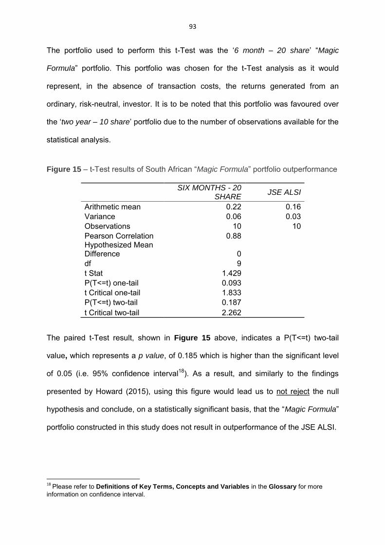
93
The portfolio used to perform this t-Test was the ‘6 month – 20 share’ “Magic
Formula” portfolio. This portfolio was chosen for the t-Test analysis as it would
represent, in the absence of transaction costs, the returns generated from an
ordinary, risk-neutral, investor. It is to be noted that this portfolio was favoured over
the ‘two year – 10 share’ portfolio due to the number of observations available for the
statistical analysis.
Figure 15 – t-Test results of South African “Magic Formula” portfolio outperformance
SIX MONTHS - 20
SHARE JSE ALSI
Arithmetic mean 0.22 0.16 Variance 0.06 0.03 Observations 10 10 Pearson Correlation 0.88
Hypothesized Mean Difference 0
df 9 t Stat 1.429 P(T<=t) one-tail 0.093 t Critical one-tail 1.833 P(T<=t) two-tail 0.187 t Critical two-tail 2.262
The paired t-Test result, shown in Figure 15 above, indicates a P(T<=t) two-tail
value, which represents a p value, of 0.185 which is higher than the significant level
of 0.05 (i.e. 95% confidence interval18). As a result, and similarly to the findings
presented by Howard (2015), using this figure would lead us to not reject the null
hypothesis and conclude, on a statistically significant basis, that the “Magic Formula”
portfolio constructed in this study does not result in outperformance of the JSE ALSI.
18
Please refer to Definitions of Key Terms, Concepts and Variables in the Glossary for more information on confidence interval.
94
Conclusion on Research Question 3
The comparable study conducted by Howard (2015) resulted in a t-Test value of
0.514 being observed. Through the adjustment to the portfolio size and portfolio
holding period the “Magic Formula”, as calculated in this study, resulted in an
increased t-Test value of 1.435 shown in Figure 15.
The higher t-Test value indicates an increased likelihood that the two means are
different, the increase in the t stat between Howard (2015) and this study indicates,
similarly to the results of Olin (2011), that the performance of the “Magic Formula”
can be enhanced by adjusting certain portfolio parameters.
In reaching a conclusion to Research Question 3 however, while adjusting certain
“Magic Formula” portfolio parameters has increased the overall performance on both
a geometric mean and risk adjusted basis, there is still, similarly to Howard (2015),
insufficient evidence to conclude that the “Magic Formula’s” outperformance of the
JSE ASLI, on a geometric mean basis, is statistically significant.

95
Other Observations in the “Magic Formula” Portfolio Composition
In determining the optimal “Magic Formula” portfolio and reviewing the performance
of the various synthetic portfolios some additional interesting insights, relating to the
portfolio composition, were established.
The most prominent insights, these being the portfolio share turnover as well as the
identification of a share selection bias, are discussed below.
Portfolio Share Turnover
Introduction
The Portfolio Share Turnover reviews the percentage of the portfolio which is
changed, on average, on the respective portfolio rebalance date.
In the section to follow, the portfolio share turnover percentage will be reviewed with
reference to the “Magic Formula” portfolio holding period, portfolio size as well as the
geometric mean return.
The portfolio holding period will be discussed in order to identify whether shares
which have been identified as being mispriced by the “Magic Formula” investment
strategy have subsequently been corrected by the market, resulting in them being
replaced by new shares in the “Magic Formula” portfolio.
Subsequently, the portfolio size shall be examined in order to establish whether the
portfolio share turnover decreases, as expected, as the portfolio size increases.
Lastly, the portfolio share turnover shall be linked to the geometric mean return in
order to establish whether there is any relationship between the realised “Magic
Formula” geometric mean return and the portfolio share turnover.

96
Results and Discussion
Portfolio Holding Period
The results of this analysis, as contained in Appendix 8 and summarised graphically
in Figure 16, are somewhat expected as the increase in holding period results in a
higher turnover percentage.
The higher portfolio share turnover which is observed as the holding period
increases implies that the combinations of the ROC and EY ratios result in the
correct identification of a mispricing. This mispricing, which is identified as being a
‘cheap’ share as a result of the EY ratio as well as a ‘good’ share as a result the
ROC ratio (Blij, 2011:7), is subsequently adjusted for in the short to medium term by
the market as indicated by the high portfolio share turnover.
Figure 16 – Average “Magic Formula” portfolio share turnover
Portfolio Size
It can be seen in Figure 16 above, with the exception of the six month portfolios, that
an increase in the portfolio size reduces the turnover percentage. This is expected
100% 100%
87% 85%
0%
20%
40%
60%
80%
100%
120%
5 Shares 10 Shares 15 Shares 20 Shares
Po
rtfo
lio S
tock
Tu
rno
ver
(%)
Portfolio Share Turnover Percentage
Six month
One year
Two year
Five year

97
because as the portfolio size increases, the likelihood of having similar shares in the
portfolio increases as you move from one period to the next.
Portfolio Turnover impact on Geometric Mean Return
When the turnover percentage is viewed in relation to the geometric mean return, as
shown in Figure 4, it would indicate that a lower portfolio turnover percentage may
result in certain shares being held for too long, reducing return. This can be seen as
the optimal portfolio size, from a geometric mean perspective, is 10 to 15 shares,
thus translating to an optimal portfolio turnover percentage of between 59% and
65%.
Table 18 – Portfolio turnover percentage generating highest mean generating returns
PORTFOLIO
SIZE TURNOVER
PERCENTAGE SIX MONTH 15 SHARES 59% ONE YEAR 10 SHARES 61% TWO YEAR 15 SHARES 65% FIVE YEAR N/A N/A
In Table 18 the five year portfolio has been excluded, as was the case under the
geometric mean return discussion, due to the limited number of observations
included within the scope of this study.
As can be seen in Figure 16 above, the six month portfolios all yielded a similar
turnover percentage with the difference between the highest and lowest share
turnovers amounting to a nominal 3% (Appendix 8).
This consistent turnover percentage, as highlighted in in the paragraph above, could
be a further reason for the low variability in geometric mean returns generated by the
six month portfolio grouping. Furthermore, since the six month portfolio turnover

98
percentages, as shown in Appendix 9, all approximate to the optimal portfolio
rebalance percentages, as set out in Table 18, it could explain the reason for all the
six month synthetic portfolios consistently outperforming the benchmark portfolio as
shown in Figure 14.
Conclusion on additional observation 1 – Portfolio Share Turnover
The investigation of the portfolio share turnover resulted in two key observations
being identified. These key observations provided further insight into the “Magic
Formula” investment strategy and the ‘optimisation’ thereof.
The first key observation was the identification that the portfolio share turnover
provides further evidence, over and above the outperformance shown in Figure 14,
in support of the “Magic Formula” investment strategy identifying share mispricing in
the market. This was found to be the case as the share turnover percentage
increases with the increase in the portfolio holding period, thus indicating an
identification and subsequent market correction of a share mispricing in the short to
medium term.
The second key observation was the identification that, similarly to the optimal
portfolio being between 10 and 20 as shown in Table 6, the returns are maximised
when the portfolio share turnover percentage falls between the ranges of 59% and
63%.
The statement, “Magic Formula” portfolio returns are maximised when the portfolio
share turnover falls between the ranges of 59% and 63%, was supported by six
months “Magic Formula” portfolios which all outperformed the benchmark portfolio
and reported a share portfolio turnover percentage approximating the portfolio

99
grouping average of 59%. Accordingly, this may be the reason for the consistent
‘excess’ risk-adjusted returns achieved by this particular portfolio grouping as shown
in Figure 14.
Selection Bias
Introduction
The second insightful observation is the possibility of a potential bias in the selection
of shares stemming from the financial information available.
As a result, in the section to follow, the potential share selection bias is reviewed in
detail with the share selection percentage being compared to the availability of
financial information. The existence of the bias will subsequently be confirmed with
reference to its statistical significance.
Should the existence be found to be statistically significant, the impact of this
observation will be reviewed with reference to the impact on this study.
Results and Discussion
Identification of share selection bias
As stated in the introduction of this section, the second insightful observation is the
possibility of a potential bias in the selection of shares. This was observed, as shown
in Figure 17, where, on average, 74% of the synthetic portfolios were made up of
shares chosen based on final results.
Comparatively, as shown in Figure 18, the breakdown of financial information, using
an overall weighted average of one year, two year and five year portfolios
rebalanced on 1 October and six month portfolios rebalanced semi-annually on 1

100
October and 1 April, indicated that only 60% of shares had final results available at
the time the selection was made.
Figure 17 – “Magic Formula” share selection percentage
Figure 18 – Percentage of publicly available information
Confirmation of share selection bias
In order to confirm this bias, as per Appendix 10, a statistical single factor ANOVA19
table was created with the purpose to test whether the means of the “Magic Formula”
share selection differed significantly from the weighted average availability of
financial results.
19
Please refer to Definitions of Key Terms, Concepts and Variables in the Glossary for more information on ANOVA table.
74%
26%
"Magic Formula" share selection
Final
Interim
60%
40%
Availability of financial information
Final
Interim

101
The results of the statistical test showed a p-value of 0.015 which, being lower than
the 5% significant level of 0.05, indicates a rejection of the null hypothesis and
accordingly it is concluded that the “Magic Formula” share selection differs
significantly from that of the available information.
Impact on the Study
A potential reason for the occurrence of this bias may be as a result of, but is not
limited to, more accurate financial information being provided at the financial year-
end due to the compulsory statutory audit which is not required for interim reporting
purposes (KPMG, 2013:16).
As a result of the “Magic Formula” using ROC and EY ratios as a basis for share
selection, which require company financial reported information, it would indicate that
the underlying bias stems from differences in market and company financial
information between interim-year results and final-year results as opposed to the
“Magic Formula” investment strategy. Consequently, for the purposes of this study,
the share selection bias falls outside the scope of the intended objectives. As such,
no further research is performed and a more thorough analysis is recommended
under Suggestions for further study below.
Conclusion on additional observation 2 – Selection Bias
The investigation into the share selection percentage (i.e. shares selected based on
final information vs. shares selected based on interim available information)
identified a bias in the shares selected skewing in favour of shares based in final
year-end information.

102
When the share selection percentage was compared to the availability of information
at the portfolio rebalance date, it resulted in a statistically significant difference which
confirmed the existence of this bias.

103
CHAPTER 5 - CONCLUSION
Research Summary
The purpose of this study was to conduct an analysis covering the effectiveness of
the “Magic Formula” investment strategy, as set out by Greenblatt (2006), in the
South African market. The scope of this analysis included all companies listed on the
JSE main board for the period between 1 October 2005 and 30 September 2015 with
the exclusion of financial services companies and companies with a market
capitalisation, at rebalance date, of less than R100 million.
It was found that the geometric mean returns generated from the “Magic Formula”
investment strategy are maximised when the portfolio size falls between 10 and 15
shares. However, with this being said, when comparing the geometric mean returns
of the portfolio to the portfolio standard deviation, a correlation of 0.93 was found to
exist. This indicated that an adjustment to the “Magic Formula” portfolio size would
not result in excess risk-adjusted returns being earned in the South African market.
From a portfolio holding period perspective, the shorter holding periods of six months
and one year yielded the highest geometric returns. However, contrastingly to the
portfolio size, each of the differing holding periods exposed the investor to differing
levels of risk with the one year and five year portfolios yielding the highest and
lowest volatilities respectively.
As a result of these findings, after calculating the respective Sharpe Ratios, the
following optimal “Magic Formula” portfolios were determined for the various investor
risk profiles:

104
- Risk-averse: A five year – 20 shares portfolio as this yields the lowest level
of volatility while still maintaining a Sharpe Ratio, i.e. greater risk-adjusted
return, in excess of the benchmark portfolio.
- Risk-seeking: A one year – 10 shares portfolio as it yields the highest
geometric mean return. It is further noted that this portfolio has a Sharpe Ratio
consistent with the benchmark portfolio.
- Risk-neutral: A two year – 10 shares portfolio or a six month – 15 shares
portfolio as these portfolios exhibit the highest risk-adjusted returns, both of
being in excess of benchmark portfolio.
When investigating the causality between the geometric mean returns generated
from the “Magic Formula” and the principles used in the share selection process it
was found, on a statistically significant basis, that the “Magic Formula” share
selection process influences the returns. As a result, this confirmed that the returns
generated by the investment were not done so randomly, and that by using the ROC
and EY ratios as a basis for share selection influences the returns generated.
Lastly, in comparing the highest geometric mean generating “Magic Formula”
portfolio with the JSE ALSI (through the use of a paired t-Test), it was concluded that
while adjusting certain portfolio parameters has increased the overall performance
on both a geometric mean and risk adjusted basis, there is still, similarly to Howard
(2015), insufficient evidence to conclude that the “Magic Formula’s” outperformance
of the JSE ASLI, on a geometric mean basis, is statistically significant at a 95%
confidence interval. This was found to be the case even though, as shown in
Appendix 12, the “Magic Formula” accumulated value over 10 years was 6.33 in
comparison to the 3.69 generated by the benchmark portfolio.

105
Conclusions and Recommendations
The analysis in this study demonstrates that the performance of the “Magic Formula”
investment strategy, and by extension value investing strategies, can be increased
when the portfolio composition is adjusted.
However, while an adjustment to the portfolio holding period and portfolio size
increased both the geometric mean return as well as the risk-adjusted return, the
increase was not sufficient to conclude on a statistical significant basis that the
“Magic Formula” investment strategy outperforms the JSE ALSI.
In applying the “Magic Formula” investment strategy to the South African market it is
suggested that, based on historical performance, a ‘five year – 20 share’ and ‘one
year – 10 share’ portfolio be constructed by a risk-averse and risk-seeking investor
respectively with a risk-neutral investor to create either a ‘two year – 10 share’ or ‘six
month – 15 share’ portfolio.
Suggestions for future research
While completing the various stages of this study, three primary areas of future
research presented themselves, namely: ‘Determining portfolio compositions which
maximise the returns of traditional value investing strategies’, ‘Combination of
alternative investment metrics’ and ‘Investigation of the share selection bias’. More
detail of these suggestions is provided below:
Determining portfolio compositions which maximise the returns of traditional value
investing strategies
The results of this study found that by altering the portfolio composition, i.e. the
holding period and the portfolio size, the risk-adjusted return could be increased.

106
Accordingly, it is suggested that for each of the traditional value investing metrics,
such as: Price-to-earnings (P/E) ratio, Dividend yield and Market-to-Book ratio etc.,
the portfolio size and portfolio holding period which results in the largest risk-
adjusted returns be determined for both the South African and global markets.
Combination of alternative investment metrics
The majority of the information currently available on value investing in South Africa
compares the benchmark portfolio to a singular metric such as the P/E ratio,
dividend yield or Market-to-Book ratio.
Further research is recommended in addressing, much like the “Magic Formula”,
whether combining various variables can add a ‘value premium’. This could be
expanded into determining which combinations of investment metrics result in
consistent long-term outperformance of the benchmark portfolio.
Investigation of the share selection bias
As identified in the results chapter of the “Magic Formula” analysis, an investigation
of the observed selection bias could be performed. More specifically, investigating
the impact, both qualitatively and quantitatively, of year-end financial information on
key investment metrics, such as ROC and EY, and performing a comparison of
these results with the results observed for interim-year financial information.
This investigation could be further extended into determining the reliability of
unaudited interim financial information through the comparison of grossed up interim
results to audited year-end financial information.

107
REFERENCES
Ahmed, P. and Nanda, S. (2000). Style investing: Incorporating growth
characteristics in value stocks. SSRN Electronic Journal
Amihud, Y. and Mendelson, H. (1986). Liquidity, asset prices and financial
policy. Financial Analysts Journal, 42(3), pp.43-48.
Aoki, M., 1984. The co-operative game theory of the firm. Oxford university press.
Asness, C.S., Frazzini, A., Israel, R. and Moskowitz, T.J. (2015). Fact, fiction, and
value investing. Journal of Portfolio Management, 42(1), pp.34-52.
Banerjee, A.V. (1992). A simple model of herd behavior, Quarterly Journal of
Economics, 107(3), pp.797-817.
Barber, B. M. and Odean, T. (2001). Boys Will Be Boys: Gender, Overconfidence,
And Common Stock Investment. The Quarterly Journal of Economics, 116(1),
pp.261-292.
Barberis, N. (2000). Investing for the long run when returns are predictable. The
Journal of Finance, 55(1), pp.225-264.
Barberis, N., Thaler, R. and Constantinides, G.M. (2003). Handbook of the
Economics of Finance. Handbook of the Economics of Finance.
Basu, S. (1977). Investment performance of Common Stocks in Relation to Their
Price-Earnings Ratios: A test of the efficient market hypothesis, The Journal of
Finance, 32(3), pp.662-682.

108
Bikhchandani, S. and Sharma, S. (2001). Herd behavior in financial markets: a
review, IMF Staff Papers, 47, pp.279–310.
Bird, R. and Whitaker, J. (2003). The performance of value and momentum
investment portfolios: Recent experience in the major European markets. Journal
of Asset Management, 4(4), pp.221-246.
Bird, R. and Casavecchia, L. (2007). Sentiment and financial health indicators for
value and growth stocks: The European experience. The European Journal of
Finance, 13(8), pp.769-793.
Black, F. (1986). “Noise”. Journal of Finance. 41(3), pp.529-543.
Blij, R.H. (2011). Back-testing Magic. Masters Dissertation. Universiteit van Tilburg.
Bodie, Z., Kane, A. and Marcus, A.J. (2009). Investments 8th Ed, McGraw-Hill
International.
Bradfield, D. and Munro, B. 2017. The number of stocks required for effective
portfolio diversification: the South African case. South African Journal of
Accounting Research, 31(1), pp.44-59.
Burger, J. (2012). An analysis of the risk free rate in the South-African capital
market. Masters Dissertation. North West University.
Business Blue-Book of South Africa. (2008). A guide to Listing Companies on the
JSE Limited. [Online]. Available at: ftp://ftp.uwc.ac.za/users/DMS/MDT-
Marion/EMS/EMS/8.%20How%20to%20do%20business%20in%20South%20Afric
a/Listing%20companies%20on%20JSE.pdf [2016, September 28]
109
Chiles, T.H. and McMackin, J.F. (1996). Integrating variable risk preferences, trust,
and transaction cost economics. Academy of management review, 21(1), pp.73-
99.
Correia, C., Flynn, D., Uliana, E. and Wormald, M. (2011). Financial Management.
Cape Town: Juta and Company Ltd.
DeBondt, W. and Thaler, R. (1985). Does the Stock Market Overreact. The Journal
of Finance, 40(3), pp.793-805.
De Long, J., Shleifer, A., Summers, L. and Waldmann, R. (1990). Noise Trader Risk
in Financial Markets. Journal of Political Economy, 98(4), pp.703-738.
Gupta, E., Preetibedi, P. and Mlakra, P. (2014). Efficient Market Hypothesis V/S
Behavioural Finance. IOSR Journal of Business and Management, 16(4), pp.56-
60.
Elton, E.J. and Gruber, M.J. (1977). Risk reduction and portfolio size: An analytical
solution. The Journal of Business, 50(4), pp.415-437.
Eltringham, S.A. (2014). Momentum on the JSE: the influence of size and
liquidity. Masters dissertation. University of the Witwatersrand.
Evans, J.L. and Archer, S.H. (1968). Diversification and the reduction of dispersion:
an empirical analysis. The Journal of Finance, 23(5), pp.761-767.
EY. (2014). Estimating risk-free rates for valuations. [Online]. Available at:
http://www.ey.com/Publication/vwLUAssets/EY-estimating-risk-free-rates-for-
valuations/$FILE/EY-estimating-risk-free-rates-for-valuations.pdf [2016, June 28]

110
Fama, E.F. (1965). Random walks in stock market prices. Financial analysts
journal, 21(5), pp.55-59.
Fama, E.F. (1970). Efficient capital markets: A review of the theory and the empirical
work. The Journal of Finance, 25(2), pp.383-417.
Fama, E.F. and French, K.R. (1992). The cross-section of expected stock returns.
Journal of Finance, 47(2), pp.427–465.
Fama, E.F. and French, K.R. (1998). Value versus Growth: The International
Evidence. Journal of Finance, 52(6), pp.1975–1999.
Fama, E.F. and French, K.R. (2012). Size, value and momentum in International
stock returns. Journal of Financial Economics, 105(3), pp.457-472.
FTSE/JSE. (2004). Guide to Calculation Methods for the FTSE/JSE Africa Index
Series. [Online]. Available at:
https://www.jse.co.za/content/JSEIndexClassificationandCodesItems/Calculation
%20Guide.pdf [2016, June 28]
Gervais, S. and Odean, T. (2001). Learning to be Overconfident. Review of Financial
Studies, 14(1):1-27
Grable, J.E. (1997). Investor risk tolerance: Testing the efficacy of demographics as
differentiating and classifying factors. Doctoral dissertation. Virginia Polytechnic
Institute and State University.
Grayswan Investments. (2013). South African Equity Market Benchmarks: A
complicated choice. [Online]. Available at:

111
http://www.grayswan.co.za/pdf/research/south_african_equity_benchmarks_marc
h_2013.pdf [2016, June 25]
Greenblatt, J. (2006). The little book that beats the market, John Wiley & Sons Inc.,
Hoboken.
Greenblatt, J. (2010). The little book that (still) beats the market, John Wiley & Sons
Inc., Hoboken.
Hoffman, A.J. (2012). Stock Return Anomalies: Evidence from the Johannesburg
Stock Exchange, Investment Analysts Journal, 75, pp.21-41.
Hoffmann, A.O., Post, T. and Pennings, J.M. (2013). Individual investor perceptions
and behavior during the financial crisis. Journal of Banking & Finance, 37, pp.60-
74.
Howard, W.F. (2015). An investment strategy based on return on capital and
earnings yield. Masters Dissertation. Stellenbosch University.
Johannesburg Stock Exchange. (2012). JSE Listing requirements. [Online] Available
at: https://www.jse.co.za/content/JSEEducationItems/Service%20Issue%2017.pdf
[2016, October 9]
Kahneman, D. and Tversky, A. (1979). Prospect theory: An analysis of decision
under risk. Econometrica: Journal of the econometric society, 47(2), pp.263-291.
KPMG. (2013). JSE Listing requirements – Quick Reference guide. [Online].
Available at:
https://www.kpmg.com/ZA/en/IssuesAndInsights/ArticlesPublications/Press-
Releases/Documents/JSE%20Listings%20brochure.pdf [2016, June 24]

112
Kruger, R. and Van Rensburg, P. (2008). Evaluating and constructing equity
benchmarks in the South African portfolio management context. Investment
Analysts Journal, 67, pp.5-18.
Larkin, P.J. (2009). Can individual investors capture the value premium. The Journal
of Business and Economics Research, 7(5), pp.25-34.
Levy, H. (1972). Portfolio performance and the investment horizon. Management
Science, 18(12), pp.B-645.
Levy, H. (1984). Measuring Risk and Performance over Alternative Investment
Horizons. Financial Analysts Journal, 40(2), pp.61-68.
Liu, W. (2006). A liquidity-augmented capital asset pricing model. Journal of financial
Economics, 82(3), pp.631-671.
MacCrimmon, K.R., Wehrung, D. and Stanbury, W.T. (1988). Taking risks. Simon
and Schuster.
Malkiel, B.G. (2003). The efficient market hypothesis and its critics. The Journal of
Economic Perspectives, 17(1), pp.59-85.
Malkiel, B.G. (2005). Reflections on the Efficient Market Hypothesis: 30 Years Later.
The Financial Review, 40(1), pp.1-9.
Miller, E.M. (1977). Risk, Uncertainty and Divergence of Opinion. The Journal of
Finance, 32(4), pp.1151-1168.
Muller, C. and Ward, M. (2013). Style-based effects on the Johannesburg Stock
Exchange: A graphical time-series approach. Investment Analysts Journal, 77,
pp.1-16.

113
Novy-Marx, R. (2013). The quality dimension of value investing. Unpublished
Manuscript. University of Rochester.
Novy-Marx, R. (2014). Quality investing. Unpublished Manuscript. University of
Rochester.
Odean, T. (1998). Volume, Volatility, Price, and Profit When All Traders are Above
Average. The Journal of Finance, 53(6), pp.1887-1934.
Olin, T. (2011). Value investing in the Finnish Market. Masters Dissertation. Aalto
university school of Economics.
Pástor, L. and Stambaugh, R. (2012). Are Stocks Really Less Volatile in the Long
Run?. Journal of Finance, 67(2), pp.431-477.
Pätäri, E. and Leivo, T. (2009). Performance of Value Strategies in the Finnish Stock
Markets, Journal of Money, Investment and Banking, 8, pp.5-24.
Pieters, R. and Zeelenberg, M. (2004). Beyond valence in customer dissatisfaction:
A review and new findings on behavioral responses to regret and disappointment
in failed services. The Journal of Business Research, 57, pp.445-455.
Reisinger, A.K. (2012). The effect of liquidity on stock returns on the JSE. Masters
dissertation. Stellenbosch University.
Ritter, J. (2003). Behavioural Finance. Pacific-Basin Finance Journal, 11, pp.429–
437.
Rousseau, R. and van Rensburg, P. (2004). Time and the payoff to value investing,
Journal of Asset Management, 4(5), pp.318-325.
114
Rousseau, R. and Zwonnikoff, C. (2002). Dynamic Benchmarking, are you using the
Right Yardstick. Deutsche Securities. Quantitative-Equity Research.
Sanlam. (2016). Minimum Disclosure Document: Global Equity Fund A USD Acc.
[Online]. Available at:
https://www.sanlam.com/productcatalog/SanlamFundFactSheets/SanlamFundFac
tSheets/SI_Sanlam%20FOUR%20Global%20Equity%20Fund%20Class%20A%2
0USD%20-%20MDD.PDF [2016, October 20]
Sareewiwatthana, P. (2011). Value Investing in Thailand: The test of basic screening
rules. International Review of Business Research Papers, 7(4), pp.1-13.
Sharpe, W.F. (1994). The sharpe ratio. The journal of portfolio management, 21(1),
pp.49-58.
Shleifer, A. and Vishny, R. (1997). The Limits of Arbitrage. Journal of Finance, 52(1),
pp.35-55.
Statman, M. (1987). How many stocks make a diversified portfolio?. Journal of
Financial and Quantitative Analysis, 22(03), pp.353-363.
Thaler, R. (1999). The End of Behavioral Finance. Financial Analysts Journal, 55(6),
pp.12-17.
Thrivent Financial. (2016). Thrivent Partner Growth Stock Portfolio. [Online].
Available at:
https://www.thrivent.com/products/files/variable/autodeploy/focus/33089GS.pdf
[2016, October 20]

115
Turkey, J. (1977). Exploratory Data Analysis. Addison-Wesley. Reading, Mass.:
Addison-Wesley Pub. Co.
Tversky, A. and Kahneman, D. (1986). Rational choice and the framing of
decisions. Journal of business, 59(4), pp.251-278.
Underhill, L. and Bradfield, D. (2014). Introstat [STA1000S Module]. Department of
Statistical Sciences, University of Cape Town.
Van Heerden, C. (2015). Is the AltX doing what it is supposed to do? An Analysis of
the JSE Alternative Exchange. Masters dissertation. Stellenbosch University.
Van Rensburg, P. and Robertson, M. (2003). Explaining the cross-section of returns
in South Africa: Attributes or factor loadings? Journal of Asset Management, 4(5),
pp.334-347.
Vovchak, V. (2014). Liquidity and Investment Horizon. Swiss Finance Institute
Research Paper, (14-02).
Wu, S. (2013). Quantitative Value Strategy Beats the Market. Masters dissertation.
University of British Columbia.
Yalҫin, K.C. (2016). Market rationality: Efficient market hypothesis versus market
anomalies. European Journal of Economic and Political Studies, 3(2), pp.23-38.
116
GLOSSARY
Definitions of Key Terms, Concepts and Variables
The following definitions of key terms, concepts and variables are provided:
- Alpha: The abnormal rate of return on a security in excess of what would be
predicted by an equilibrium model like ‘CAPM’ or ‘APT’.
- ANOVA: Analysis of variance (ANOVA) is an analysis tool used in statistics. It
summarises the sources of variation (Underhill and Bradfield, 2014:299)
- Behavioural finance: Models of financial markets that emphasise
implications of psychological factors impacting on investor behaviour.
- Bid-Ask spread: The difference between a dealers bid and asked price.
- Confidence Interval: A confidence interval measures the probability that a
population parameter will fall between two set values (Underhill and Bradfield,
2014:178)
- Dividend Yield: The percentage rate of return provided by a shares dividend
payments.
- Earnings Yield (EY): The ratio of earnings to price (i.e. The earnings yield is
the inverse of the price earnings ratio as mentioned above).
- Efficient market hypothesis (EMH): The prices of securities fully reflect
available information. Investors buying securities in an efficient market should
expect to obtain an equilibrium rate of return.
- Growth Shares: A growth share is a share in a company whose earnings are
expected to grow at an above-average rate relative to the market (Thrivent
Financial, 2016:1)
- Liquidity: The speed and ease with which an asset can be converted into
cash.

117
- Net Debt: Net Debt is determined as Short term debt plus Long term debt
less Cash and cash equivalents (Blij, 2011).
- Net fixed assets: Net fixed assets is determined as Total Assets less Total
current assets less total goodwill (Blij, 2011).
- Net working capital (NWC): Net working capital is all current assets less
current liabilities. It is used to measure the liquidity of a business (Blij, 2011).
- Price Earnings Ratio: The ratio of a shares price to its earnings per a share.
- Random Walk: Describes the notion that share price changes are random
and unpredictable.
- Return on Capital (ROC): Return on Capital is a financial ratio that measures
the efficiency with which capital is employed (Blij, 2011).
- Risk-Free Rate: The interest rate which can be earned with certainty.
- Risk Premium: An expected return in excess of that on risk-free securities.
The premium provides compensation for the risk of an investment.
- Sharpe’s Ratio: Reward to volatility ratio, ratio of portfolio excess return to
standard deviation.
- Statistical Outliers: An outlier is an observation strikingly far from some
central value. It is an unusual value relative to the bulk of the data (Tukey,
1977)
- Statistical Significance: This relates to how we infer or draw conclusions
from data (Underhill and Bradfield, 2014:182). It relates to the likelihood that a
relationship between 2 or more variables is caused by something other than a
random chance.

118
- t-Test: This refers to the analysis of two population’s means through the use
of statistical examination. The t-tests is used for comparing means of two
populations (Underhill and Bradfield, 2014:211)
- Value Investing: This is a strategy of selecting shares that trade for less than
their intrinsic values. Value investors actively seek shares that they believe
the market has undervalued. They believe the market overreacts to good and
bad news, resulting in share price movements that do not correspond with the
company's actual long-term fundamentals. The result is an opportunity for
value investors to profit by buying when the price is deflated (Sanlam, 2016:1)
The definitions of key terms, concepts and variables as set out above is intended to
provide the reader with additional, explanatory, information on technical concepts
contained herein.
Unless otherwise indicated, the information contained in the glossary was sourced in
accordance with the reference below:
Bodie, Z., Kane, A. and Marcus, A.J., 2009. Investments 8th Ed, McGraw-Hill
International.

119
5 SHARES 10 SHARES 15 SHARES 20 SHARES 5 SHARES 10 SHARES 15 SHARES 20 SHARES
30
SHARES¹⁷ 5 SHARES 10 SHARES 15 SHARES 20 SHARES 5 SHARES 10 SHARES 15 SHARES 20 SHARES
2005 to 2006 21% 33% 35% 36% 37% 36% 43% 35% 33% 36%2006 to 2007 68% 70% 78% 73% 61% 52% 48% 45% 46% 37%2007 to 2008 -8% -24% -21% -22% -20% -26% -24% -23% -24% -18%2008 to 2009 25% 11% 13% 14% 13% 9% 5% 7% 3% 8%2009 to 2010 -2% 4% 10% 13% 9% 10% 10% 11% 19% 21%2010 to 2011 24% 9% 14% 20% 18% 4% 11% 21% 19% 4%2011 to 2012 23% 31% 38% 35% 10% 48% 39% 46% 41% 24%2012 to 2013 39% 39% 32% 31% 18% 45% 40% 35% 28% 27%2013 to 2014 -5% 21% 17% 11% -3% 30% 15% 13% 12% 15%2014 to 2015 -2% 5% 6% 6% 37% 19% 18% 14% 10% 5%
Geometric Mean 16% 17% 19.8% 19% 16% 20.3% 19% 18% 17% 13% 19% 20% 17% 5% 7% 10% 13% 15%
Initial Portfolio Value 1,000 1,000 1,000 1,000 1,000 1,000 1,000 1,000 1,000 1,000 1,000 1,000 1,000 1,000 1,000 1,000 1,000 1,691
Ending Portfolio Value 4,525 4,974 6,106 5,920 4,365 6,374 5,484 5,437 4,763 3,514 5,572 6,099 4,719 1,614 2,034 2,703 3,428 6,695
Compound Annual Growth Rate 16% 17% 20% 19% 16% 20% 19% 18% 17% 13% 19% 20% 17% 5% 7% 10% 13% 15%
5% 42% 82%64%
24%36% 53%
26%
0%
94% 91%-16%
38%
9%
-21%
33%
67%
-19%
RETURN
FIVE YEARS
105% 108%
SIX MONTHS¹⁶
JSE ALSI
ONE YEAR TWO YEARS
127%
62% 89%
161%
-13%
28%
62%
30%
APPENDIXES
Appendix 1 – Return generated by the “Magic Formula” investment strategy on the South African market
Six month portfolios20
One year – 30 share portfolio21
20
The six month portfolios, represented in the table above, all present the annual equivalent return which is achieved through semi-annual rebalancing on 1 April and 1 October. The annual equivalent is shown in order to allow for easy comparison with the respective one year portfolios. 21 The one year – 30 share portfolio is highlighted above as the purpose of this synthetic “Magic Formula” portfolio was, contrastingly to the other portfolios shown above, to allow for a direct comparison with a comparable study performed in the South African market.

120
Appendix 2 – SENS announcement for the Share Split of Combined Motor Holdings
(JSE:CMH)
Source: McGregor BFA
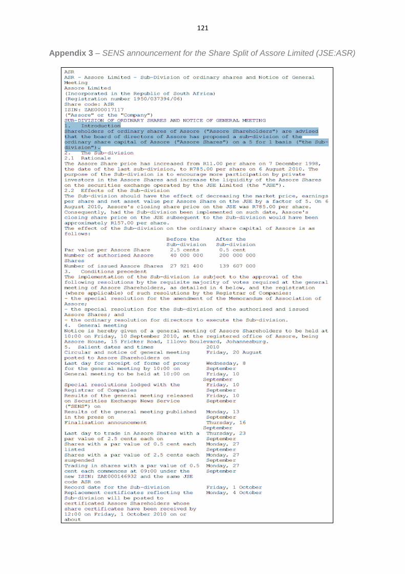
121
Appendix 3 – SENS announcement for the Share Split of Assore Limited (JSE:ASR)

122
Source: McGregor BFA

123
Appendix 4 – “Magic Formula” portfolio annual return generated under an
alternative study
Source: Howard, 2015:38
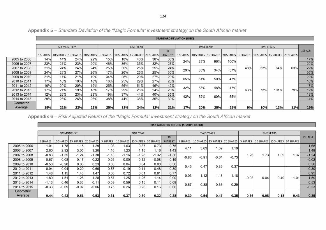
124
5 SHARES 10 SHARES 15 SHARES 20 SHARES 5 SHARES 10 SHARES 15 SHARES 20 SHARES
30
SHARES¹⁷ 5 SHARES 10 SHARES 15 SHARES 20 SHARES 5 SHARES 10 SHARES 15 SHARES 20 SHARES
2005 to 2006 14% 14% 24% 22% 15% 18% 40% 38% 33% 17%2006 to 2007 23% 21% 23% 20% 46% 36% 35% 32% 27% 20%2007 to 2008 21% 24% 24% 24% 25% 30% 25% 25% 24% 22%2008 to 2009 24% 28% 27% 26% 17% 26% 26% 25% 30% 36%2009 to 2010 21% 17% 21% 19% 34% 25% 29% 27% 29% 22%2010 to 2011 17% 16% 19% 18% 16% 25% 29% 27% 26% 16%2011 to 2012 10% 20% 20% 19% 25% 56% 51% 46% 42% 17%2012 to 2013 17% 21% 19% 18% 17% 29% 26% 24% 23% 12%2013 to 2014 12% 26% 23% 23% 19% 37% 44% 40% 35% 13%2014 to 2015 29% 26% 26% 26% 38% 44% 38% 35% 39% 14%
Geometric Average 19% 21% 23% 21% 25% 32% 34% 32% 31% 17% 20% 25% 25% 9% 10% 13% 11% 19%
50% 47%
63% 73% 101% 79%32%
24% 28% 96% 100%
48%
53% 48% 47%
42% 52%
64% 63%29% 33%
60% 55%
53%34% 37%
65% 51%
SIX MONTHS¹⁶ ONE YEAR TWO YEARS FIVE YEARS
STANDARD DEVIATION (RISK)
JSE ALSI
5 SHARES 10 SHARES 15 SHARES 20 SHARES 5 SHARES 10 SHARES 15 SHARES 20 SHARES
30
SHARES¹⁷ 5 SHARES 10 SHARES 15 SHARES 20 SHARES 5 SHARES 10 SHARES 15 SHARES 20 SHARES
2005 to 2006 1.01 1.78 1.15 1.29 1.98 1.63 0.87 0.73 0.75 1.682006 to 2007 2.60 2.92 3.05 3.20 1.16 1.23 1.15 1.16 1.43 1.482007 to 2008 -0.83 -1.35 -1.24 -1.30 -1.18 -1.16 -1.28 -1.32 -1.36 -1.242008 to 2009 0.67 0.08 0.17 0.22 0.26 0.00 -0.12 -0.08 -0.19 -0.022009 to 2010 -0.50 -0.28 0.06 0.23 0.00 0.04 0.04 0.08 0.36 0.562010 to 2011 0.94 0.04 0.29 0.66 0.57 -0.19 0.11 0.48 0.39 -0.302011 to 2012 1.48 1.15 1.46 1.47 0.06 0.72 0.61 0.81 0.77 0.952012 to 2013 1.89 1.51 1.26 1.28 0.57 1.25 1.26 1.14 0.90 1.592013 to 2014 -1.13 0.46 0.36 0.11 -0.59 0.59 0.15 0.11 0.09 0.532014 to 2015 -0.33 -0.09 -0.07 -0.06 0.75 0.26 0.26 0.16 0.06 -0.23
Geometric Average 0.44 0.43 0.51 0.53 0.31 0.37 0.30 0.32 0.28 0.30 0.54 0.47 0.35 -0.36 -0.08 0.18 0.43 0.35
1.13 1.18
0.67 0.88
0.47 0.39 0.37
-0.03 0.040.03
1.26
1.12
RISK ADJUSTED RETURN (SHARPE RATIO)
JSE ALSI
SIX MONTHS¹⁶ ONE YEAR TWO YEARS FIVE YEARS
0.36 0.29
1.73 1.39 1.37-0.86 -0.91 -0.64 -0.73
0.45
4.11 3.63 1.59 1.19
0.40 1.01
Appendix 5 – Standard Deviation of the “Magic Formula” investment strategy on the South African market
Appendix 6 – Risk Adjusted Return of the “Magic Formula” investment strategy on the South African market

125
Appendix 7 – Single Factor ANOVA table and related Equation showing consistent returns for the 6 month holding period grouping
H0: µ1 = µ2 = µ3 = µ4
Where:
µ = Mean Return
Anova: Single Factor
SUMMARY
Groups Count Sum Average Variance SIX MONTH - 5 SHARES 10 1.831 0.183 0.056
SIX MONTH - 10 SHARES 10 1.990 0.199 0.065 SIX MONTH - 15 SHARES 10 2.222 0.222 0.067
SIX MONTH - 20 SHARES 10 2.172 0.217 0.061
ANOVA Source of Variation SS df MS F P-value F crit
Between Groups 0.00961561 3 0.003 0.052 0.984 2.866
Within Groups 2.233934992 36 0.062 Total 2.243550601 39
As p > 0.05, cannot reject H0
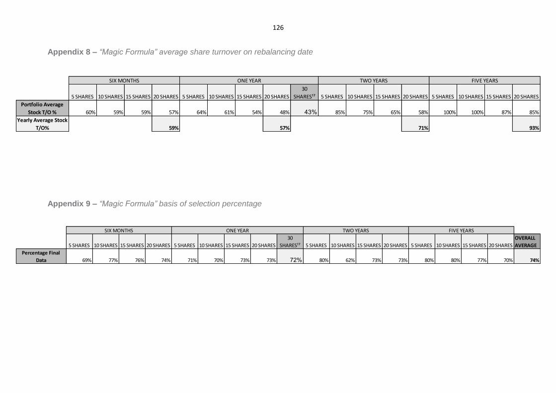
126
Appendix 8 – “Magic Formula” average share turnover on rebalancing date
Appendix 9 – “Magic Formula” basis of selection percentage
5 SHARES 10 SHARES 15 SHARES 20 SHARES 5 SHARES 10 SHARES 15 SHARES 20 SHARES
30
SHARES¹⁷ 5 SHARES 10 SHARES 15 SHARES 20 SHARES 5 SHARES 10 SHARES 15 SHARES 20 SHARES
OVERALL
AVERAGE
Percentage Final
Data 69% 77% 76% 74% 71% 70% 73% 73% 72% 80% 62% 73% 73% 80% 80% 77% 70% 74%
SIX MONTHS ONE YEAR TWO YEARS FIVE YEARS
5 SHARES 10 SHARES 15 SHARES 20 SHARES 5 SHARES 10 SHARES 15 SHARES 20 SHARES
30
SHARES¹⁷ 5 SHARES 10 SHARES 15 SHARES 20 SHARES 5 SHARES 10 SHARES 15 SHARES 20 SHARES
Portfolio Average
Stock T/O % 60% 59% 59% 57% 64% 61% 54% 48% 43% 85% 75% 65% 58% 100% 100% 87% 85%
Yearly Average Stock
T/O% 59% 57% 71% 93%
SIX MONTHS ONE YEAR TWO YEARS FIVE YEARS
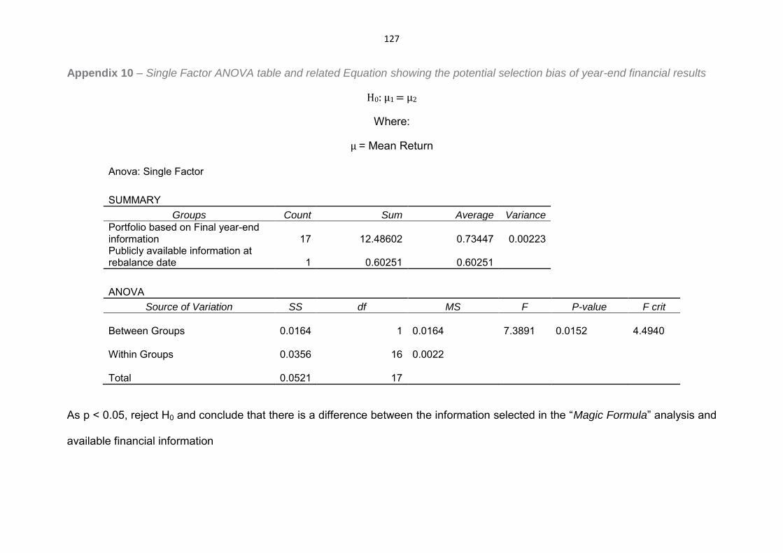
127
Appendix 10 – Single Factor ANOVA table and related Equation showing the potential selection bias of year-end financial results
H0: µ1 = µ2
Where:
µ = Mean Return
Anova: Single Factor
SUMMARY Groups Count Sum Average Variance
Portfolio based on Final year-end information 17
12.48602
0.73447
0.00223
Publicly available information at rebalance date 1
0.60251
0.60251
ANOVA
Source of Variation SS df MS F P-value F crit
Between Groups 0.0164 1
0.0164
7.3891
0.0152
4.4940
Within Groups 0.0356 16
0.0022
Total
0.0521 17
As p < 0.05, reject H0 and conclude that there is a difference between the information selected in the “Magic Formula” analysis and
available financial information

128
Appendix 11 – JSE ALSI TRI, benchmark portfolio, relative performance over the explicit period of the study
Appendix 12 – Cumulative performance of top performing “Magic Formula” portfolios
010002000300040005000600070008000
01-O
ct-0
501
-Jan
-06
01-A
pr-0
601
-Jul
-06
01-O
ct-0
601
-Jan
-07
01-A
pr-0
701
-Jul
-07
01-O
ct-0
701
-Jan
-08
01-A
pr-0
801
-Jul
-08
01-O
ct-0
801
-Jan
-09
01-A
pr-0
901
-Jul
-09
01-O
ct-0
901
-Jan
-10
01-A
pr-1
001
-Jul
-10
01-O
ct-1
001
-Jan
-11
01-A
pr-1
101
-Jul
-11
01-O
ct-1
101
-Jan
-12
01-A
pr-1
201
-Jul
-12
01-O
ct-1
201
-Jan
-13
01-A
pr-1
301
-Jul
-13
01-O
ct-1
301
-Jan
-14
01-A
pr-1
401
-Jul
-14
01-O
ct-1
401
-Jan
-15
01-A
pr-1
501
-Jul
-15
JSE ALSI TRI
Index close
0.001.002.003.004.005.006.007.00
2005 to2006
2006 to2007
2007 to2008
2008 to2009
2009 to2010
2010 to2011
2011 to2012
2012 to2013
2013 to2014
2014 to2015
Cumulative performance of top performing "Magic Formula" portfolios
Six year - 15ShareOne Year - 10ShareTwo year - 15ShareFive year - 20ShareJSE ALSI TRI
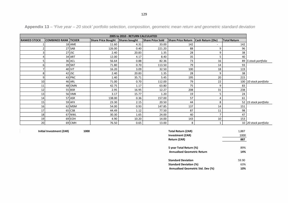
129
RANKED STOCK COMBINED RANK TICKER Share Price Bought Shares bought Share Price Sold Share Price Return Cash Return (Div) Total Return
1 18 AME 11.60 4.31 33.00 142 - 142
2 27 SAB 126.00 0.40 221.20 88 9 96
3 27 JSC 2.40 20.83 1.35 28 9 38
4 34 ART 12.00 4.17 8.40 35 5 40
5 36 ACL 56.64 0.88 82.36 73 16 89 5 stock portfolio
6 39 SNT 71.80 0.70 113.50 79 14 93
7 40 IVT 16.20 3.09 32.50 100 18 119
8 42 JSC 2.40 20.83 1.35 28 9 38
9 43 PNC 1.40 35.71 5.45 195 20 215
10 46 ARL 71.00 0.70 112.00 79 22 100 10 stock portfolio
11 48 OMN 42.75 1.17 63.80 75 9 83
12 55 BSR 2.95 16.95 12.27 208 31 238
13 56 VMK 3.17 15.77 1.20 19 5 24
14 57 ASR 138.00 0.36 157.00 57 4 61
15 59 AFX 23.30 2.15 20.50 44 8 52 15 stock portfolio
16 62 MSM 54.00 0.93 147.85 137 14 151
17 65 CSB 44.49 1.12 77.50 87 11 98
18 67 NWL 30.30 1.65 24.00 40 7 47
19 69 EOH 4.90 10.20 14.00 143 10 153
20 69 CMH 76.50 0.65 13.00 8 1 10 20 stock portfolio
Initial Investment (ZAR) 1000 Total Return (ZAR) 1,887
Investment (ZAR) 1000
Return (ZAR) 887
5 year Total Return (%) 89%
Annualised Geometric Return 14%
Standard Deviation 59.90
Standard Deviation (%) 63%
Annualised Geometric Std. Dev (%) 10%
2005 to 2010 - RETURN CALCULATED
Appendix 13 – ‘Five year – 20 stock’ portfolio selection, composition, geometric mean return and geometric standard deviation

130
RANKED STOCK COMBINED RANK TICKER Share Price Bought Shares bought Share Price Sold Share Price Return Cash Return (Div) Total Return
1 13 SSK 10.90 8.66 4.00 35 6 41
2 32 AER 1.50 62.91 2.75 173 33 206
3 36 WBO 124.00 0.76 111.77 85 14 99
4 40 VMK 1.20 78.64 0.42 33 27 60
5 47 KIO 368.95 0.26 77.87 20 44 64 5 stock portfolio
6 51 ESR 2.16 43.69 0.24 10 - 10
7 53 RBX 22.82 4.14 17.40 72 15 87
8 56 AEN 26.38 3.58 7.00 25 4 29
9 61 PWK 17.75 5.32 28.44 151 15 166
10 61 TPC 11.19 8.43 22.50 190 37 227 10 stock portfolio
11 62 PNC 5.45 17.31 12.79 221 17 239
12 63 BIL 225.90 0.42 223.39 93 23 116
13 63 CIL 5.60 16.85 33.38 562 - 562
14 64 ELI 1.68 56.17 0.70 39 6 45
15 70 GRF 36.90 2.56 19.10 49 8 57 15 stock portfolio
16 71 ELR 13.90 6.79 30.00 204 27 231
17 72 BTI 258.58 0.36 820.77 300 36 335
18 74 RLF 1.41 66.92 3.26 218 20 238
19 74 AME 33.00 2.86 99.85 286 27 313
20 83 MTA 10.25 9.21 29.00 267 35 302 20 stock portfolio
Initial Investment (ZAR) 1,887 Total Return (ZAR) 3,428
Investment (ZAR) 1887
Return (ZAR) 1,540
5 year Total Return (%) 82%
Annualised Geometric Return 13%
Column1
Standard Deviation 135.17
Standard Deviation (%) 79%
Annualised Geometric Std. Dev (%) 12%
2010 to 2015 - RETURN CALCULATED


![Content Marketing & Influencers: the magic formula [Webinar]](https://static.fdocuments.net/doc/165x107/559eb3f81a28abd26a8b480c/content-marketing-influencers-the-magic-formula-webinar.jpg)