Maejo Int. J. Sci. Technol 2020 14(02), 156-165 Maejo ...

Maejo Int. J. Sci. Technol. 2020, 14(02), 156-165

Maejo International Journal of Science and Technology

ISSN 1905-7873

Available online at www.mijst.mju.ac.th Technical Note

Determination of normal height of Chornohora summits by precise modern measurement technique

Jacek Kudrys, Małgorzata Busko, Krystian Kozioł and Kamil Maciuk* Department of Integrated Geodesy and Cartography, Faculty of Mining Surveying and Environmental Engineering, AGH University of Science and Technology, al. Mickiewicza 30, 30-059 Krakow, Poland * Corresponding author, e-mail: [email protected] Received: 14 April 2019 / Accepted: 18 May 2020 / Published: 11 June 2020 Abstract: The heights of the two Ukrainian peaks - Hoverla and Pip Ivan located in the Chornohora mountain range - were determined by using Global Navigation Satellite System observations and a global quasi-geoid model. The height of Hoverla, the highest Ukrainian summit, 2056.0 ± 0.5 m, and that of Pip Ivan is 2019.4 ± 0.5 m. The results are several metres lower than the official altitudes. Keywords: Chornohora mountain, Global Navigation Satellite System, mountain height determination, Hoverla, Pip Ivan _______________________________________________________________________________________ INTRODUCTION The highest peak of the Chornohora Mountains, a part of the Outer Eastern Carpathians, the highest mountain range in the Ukraine, is Hoverla (2,061 m, Figures 1, 2) [1]. Pip Ivan (2,022 m) is the third highest Ukrainian peak, after Hoverla and Brebeneskul [2]. Only six Ukrainian mountains reach over 2,000 m and all of them are located in the Chornohora Mountains. The other three are Petros, Rebra and Hutyn Tomnatyk [4]. The Chornohora Mountains are a widely studied area in the Earth sciences [5–11], but the authors of this paper did not find any elaborations concerning the determination of the height of any of these Ukrainian peaks. Formerly the Chornohora mountain range was the historical border of Galicia and Lodomeria and the Polish-Czechoslovak border [12]. Currently it is the border between two Ukrainian districts - Transcarpathian and Ivano-Frankivsk. The reason for our research was a certain inaccuracy and uncertainty regarding the heights of Hoverla and Pip Ivan based on the historical cartographic and geographic materials.


157

Figure 1. Location of the Ukrainian two-thousanders [3]

Figure 2. Summits of Hoverla (left) and Pip Ivan (right)

CHORNOHORA HEIGHTS When analysing historical cartographic materials concerning the heights of the Chornochora peaks, Austria-Hungarian maps from 1855-1914 [13] and Polish maps from 1930 – 1933 [13] were found. In addition, the Chornohora’s peak heights are given in a book [14]. This book contains three different heights of Hoverla, given in metres, feet and fathoms, while the height of Pip Ivan appears only once. Table 1 contains a summary from all the above-mentioned source materials. The heights presented in Table 1 vary between 2050.7 - 2058.0 m (difference 7.3 m) for Hoverla and 2013.1 - 2026.0 m (difference 12.9 m) for Pip Ivan. The height of Hoverla expressed in feet (7,200 ft = 2,276.0 m) is most likely incorrect. The altitude differences are results of the adopted reference level, measurement accuracy and the selected method of unit conversion (Figure 3).


158

Table 1. Historical heights of Hoverla and Pip Ivan

Source Hoverla Pip Ivan

Name Year Non- metric Metric Non-metric Metric

Austria-Hungarian map [13] 1855 1,081.3 vf1 2,050.7 m 1,061,5 vf 2,013.1 m 1873 1,082.0 vf 2,052.0 m 1,062.0 vf 2,014.1 m 1876 - 2,058.0 m - 2,026.0 m

Słownik geograficzny Królestwa Polskiego (Geographical dictionary of the Kingdom of Poland) [14]

1880

- 2,058.0 m -

2,026.0 m 1,081.3 vf 2,050.7 m - 7,200 ft2 2,276.0 m -

Austria-Hungarian map [13] 1914 - 2,057.0 m - 2,026.0 m Polish map [13] 1930 - 2,058.0 m - 2,026.0 m Polish map [13] 1933 - 2,058.0 m - 2,022.0 m This paper’s results 2018 - 2,055.0 m - 2,019.4 m

1 Vienna fathom = 1.896484 m [14], 2 Viennese foot = 0.3161 m [14]

Figure 3. Part of Austria-Hungarian map of Hoverla and Pip Ivan from 1855 and 1914 [13]

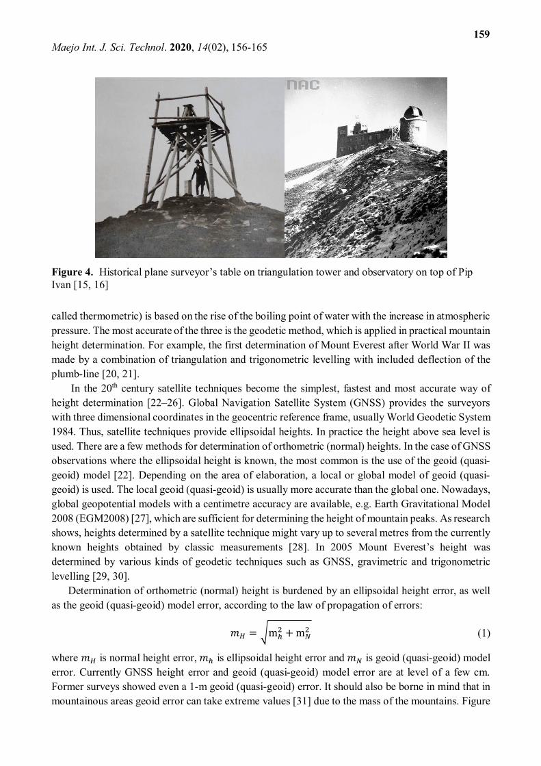
Figure 4 presents historical pictures of Pip Ivan. The left picture shows the triangulation tower where probably the heights were referenced before World War II. The right picture shows the triangulation tower with the Bilyi Slon observatory in the background. The height of the triangulation tower in Figure 4 is about 3 - 4 m and probably some of the determined Pip Ivan heights were not reduced to the terrain. On the Hoverla top there is a concrete monument (Figure 7B) which is also a former triangulation point. The heights presented in Table 1 might also refer to the top of the monument. METHODS OF PEAK HEIGHT DETERMINATION There were three different methods of determining mountain heights above sea level or other adopted reference surface: the geodetic method, the barometric method and the boiling point method [17]. The geodetic method is based on levelling [18] and triangulation (angular-linear intersections). The barometric method is based on the air pressure difference between sea level and the top of the mountain; this method is rarely used, rather as a scientific issue [19]. The boiling point method (also


159

Figure 4. Historical plane surveyor’s table on triangulation tower and observatory on top of Pip Ivan [15, 16]

called thermometric) is based on the rise of the boiling point of water with the increase in atmospheric pressure. The most accurate of the three is the geodetic method, which is applied in practical mountain height determination. For example, the first determination of Mount Everest after World War II was made by a combination of triangulation and trigonometric levelling with included deflection of the plumb-line [20, 21].

In the 20th century satellite techniques become the simplest, fastest and most accurate way of height determination [22–26]. Global Navigation Satellite System (GNSS) provides the surveyors with three dimensional coordinates in the geocentric reference frame, usually World Geodetic System 1984. Thus, satellite techniques provide ellipsoidal heights. In practice the height above sea level is used. There are a few methods for determination of orthometric (normal) heights. In the case of GNSS observations where the ellipsoidal height is known, the most common is the use of the geoid (quasi-geoid) model [22]. Depending on the area of elaboration, a local or global model of geoid (quasi-geoid) is used. The local geoid (quasi-geoid) is usually more accurate than the global one. Nowadays, global geopotential models with a centimetre accuracy are available, e.g. Earth Gravitational Model 2008 (EGM2008) [27], which are sufficient for determining the height of mountain peaks. As research shows, heights determined by a satellite technique might vary up to several metres from the currently known heights obtained by classic measurements [28]. In 2005 Mount Everest’s height was determined by various kinds of geodetic techniques such as GNSS, gravimetric and trigonometric levelling [29, 30]. Determination of orthometric (normal) height is burdened by an ellipsoidal height error, as well as the geoid (quasi-geoid) model error, according to the law of propagation of errors: 푚 = m + m (1)

where 푚 is normal height error, 푚 is ellipsoidal height error and 푚 is geoid (quasi-geoid) model error. Currently GNSS height error and geoid (quasi-geoid) model error are at level of a few cm. Former surveys showed even a 1-m geoid (quasi-geoid) error. It should also be borne in mind that in mountainous areas geoid error can take extreme values [31] due to the mass of the mountains. Figure


160

5 presents height anomaly at the Chornohora mountains region on the basis of the EGM2008 geopotential model.

Figure 5. EGM2008 height anomaly at Chornohora area (scale in metre) [32]

METHODOLOGY The GNSS technique was chosen to determine the height of the summit of Pip Ivan and Hoverla. Although the GNSS technique is very convenient and relatively precise in height determination, it gives results in ellipsoidal coordinates, so a determined height is referred to ellipsoid, not to the mean sea level (reference level - geoid in orthometric height system, and quasi-geoid in a normal height system) [33]. The difference between the ellipsoid and geoid is the geoid height 푁 in the orthometric height system. The difference between ellipsoidal height and height above sea level is called height anomaly in the normal height system (Figure 6). The height anomaly in the normal height system, usually marked as 휁, is in the range of -100 to 100 m over the whole Earth. In the Chornohora region the height anomaly is about 36 m (Figure 5). The normal height (퐻) determination consists of the ellipsoidal height (ℎ) measurement, usually with GNSS techniques, and the determination of height anomaly according to a simple formula: 퐻 = ℎ − 휁 . (2) The height anomaly 휁 may be obtained from global or regional geoid models.


161

Figure 6. Ellipsoidal height (h), normal height (H, HAUX) and height anomaly (ζ)

MEASUREMENTS The measurements were carried out by a two two-person measuring team with geodetic instruments (GNSS receiver, precision leveller). The base of border mark no. 16 on Pip Ivan (Figures 7D, 8) on the west side of the observatory was adopted as the peak. It is the same border mark as shown in Figure 4. In the case of Hoverla, a concrete mark with a notched cross was adopted as the highest point (Figures 7C, 8). The highest summit points are with high sky obstructions on Pip Ivan and in the location of the main tourist route on Hoverla. Therefore, for the GNSS measurements session, auxiliary points with maximum exposure of the horizon were chosen. The auxiliary points were located a few metres next to the highest points (Hoverla - Figure 7A, Pip Ivan - Figure 8E). GNSS measurements at auxiliary points using a Leica GS16 were made on 13 September 2018 during a single 5-hour measuring session, between 8:00 - 13:00 GMT. The observations were made with a 1-sec. interval and 0º elevation cut-off angle. After the GNSS session, the height difference between the auxiliary and highest points was determined by geometric levelling using a Leica Sprinter leveller. The normal height system is legally operative on Ukrainian territory; thus the EGM2008 quasi-geoid model and height anomaly values are used for the calculations. RESULTS The geodetic coordinates of the auxiliary points were determined using Precise Point Positioning (PPP) technique in the International Terrestrial Reference Frame (ITRF2014 realization). Based on ellipsoidal coordinates (휑, 휆) and the EGM2008 model, the height anomaly of these points was calculated using the EGM2008 Harmonic Synthesis Program [27]. The normal heights (above sea level) of the auxiliary points were calculated from equation (2). The distance between the auxiliary and highest points was a few metres so height anomalies were adopted as being the same. The results are presented in Table 2.


162

Figure 7. Hoverla (top) and Pip Ivan (bottom) summits during the experiment

Figure 8. Geodetic marks on the top of Pip Ivan (left) and Hoverla (right)


163

Table 2. Results of peak height determination

ℎ (m) 휁 (m) 푑퐻 (m) 퐻 (m)

Pip Ivan 2053.527 36.805 2.634 2019.356 Hoverla 2092.239 36.507 0.228 2055.960

Note: ℎ - ellipsoidal height of the auxiliary point, 휁 - height anomaly, 푑퐻 - difference from levelling between auxiliary point and geodetic mark, 퐻 - summit normal height

For result verification, differential processing of the Pip Ivan-Hoverla baseline was also performed. The differences of vector components dx, dy, dz from the differential method, compared with those obtained by PPP technique, did not exceed 2 cm. In accordance with the measurement method and the geoid model used, the accuracy of the height determination can be estimated as the sum of three error components: auxiliary point height from GNSS measurement (푚 ) = 0.05 푚, height anomaly from EGM2008 model (푚 ) = 0.50 푚 [34], and height difference from levelling (푚 ) = 0.001 푚. According to the uncertainty propagation, the summit height determination error may be represented by equation (3) - a modified formula of (1): 푚 = 푚 + 푚 + 푚 . (3) The obtained accuracy of the summit height determination (푚 ) is about 0.5 m. Among all of the errors - GNSS measurement, levelling and height anomaly model - the last one is significant; the others may be considered negligibly small without affecting the accuracy of the height determination. CONCLUSIONS

The PPP method is accurate enough for ellipsoidal height determination. A comparison of the PPP results with post-processed Pip Ivan-Hoverla baseline shows compatibility at a level of several centimetres. Global geoid models for the Chornohora Mountains enable us to determine the summit heights with an accuracy of 0.5 m. ACKNOWLEDGEMENT The article was created as part of the statutory research of AGH No. 16.16.150.545. REFERENCES 1. M. Racický, J. Ostrolucký, M. Puchnerová and L. Zboril, “Environmental restoration of surface

and groundwater in the Upper Tisza basin”, in “Restoration of Degraded Rivers: Challenges, Issues and Experiences” (Ed. D. P. Loucks), Springer, Dordrecht, 1998, Vol.39, pp.229-242.

2. C. Pachschwöll, M. Puşcaş and P. Schönswetter, “Distribution of Doronicum clusii and D. stiriacum (Asteraceae) in the Alps and Carpathians”, Biologia, 2011, 66, 977-987.

3. OpenStreetMap Contributors, “OpenStreetMap”, 2004, https://www.openstreetmap.org (Accessed: April 2019).

4. P. Paparyha, L. Pipash, V. Shmilo and A. Veklyuk, “Hydrochemical status of streams and rivers of the upper Tysa River basinin the Ukrainian Carpathians”, in “Transylvanian Review of


164

Systematical and Ecological Research - The Upper Tisa River Basin” , Vol. 11 (Ed. D. Bănăduc, B. Prots and A. Curtean-Bănăduc), University of Sibiu, Sibiu, pp.47-52.

5. D. Bernátová, J. Májovský, J. Kliment and J. Topercer Jr., “Taxonomy and distribution of Poa carpatica in the Western Carpathians”, Biologia, 2006, 61, 387-392.

6. J. A. Szabó, “Decision supporting hydrological model for river basin flood control”, in “Digital Terrain Modelling” (Ed. R. J. Peckham and G. Jordan), Springer, Berlin, 2007, pp.145-182.

7. G. Timár and G. Gábris, “Estimation of water conductivity of the natural flood channels on the Tisza flood-plain, the Great Hungarian Plain”, Geomorphol., 2008, 98, 250-261.

8. D. Lóczy, M. Stankoviansky and A. Kotarba (Ed.), “Recent Landform Evolution, the Carpatho-Balkan-Dinaric Region”, Springer, Berlin, 2012.

9. M. Árvai, I. Popa, M. Mîndrescu, B. Nagy and Z. Kern, “Dendrochronology and radiocarbon dating of subfossil conifer logs from a peat bog, Maramureş Mts, Romania”, Quat. Int., 2016, 415, 6-14.

10. K. Widawski and J. Wyrzykowski, “The geography of Tourism of Central and Eastern European Countries”, 2nd Edn., Springer, Cham, 2017.

11. Y. Didukh, I. Kontar and A. Boratynski, “Phytoindicating comparison of vegetation of the Polish Tatras, the Ukrainian Carpathians, and the Mountain Crimea”, in “Geographical Changes in Vegetation and Plant Functional Types” (Ed. A. M. Greller, K. Fujiwara and F. Pedrotti), Springer International Publishing, Basel, 2018, pp.185-210.

12. S. Apunevych, O. Lohvynenko, B. Novosyadlyj and M. Kovalchuk, “First astronomical observatory in Lviv”, Kinemat. Phys. Celest. Bodies, 2011, 27, 265-272.

13. A. Bargański, I .Drecki, J. Kucharski, H. Neugass, K. Niecikowski, M. Zieliński and T. Pluciński, “Archiwum map wojskowego Instytutu Geograficznego”, 1919-1939, http://mapywig.org (Accessed: April 2019).

14. F. Sulimierski, B. Chlebowski and W. Walewski, “Słownik geograficzny Królestwa Polskiego i innych krajow słowiańskich”, Druk Wieku, Warszawa, 1880.

15. L. Rymarowicz, “Powrót słupa granicznego na Pop Iwana”, 2018, http://karpaccy.pl (Accessed: April 2019).

16. N. A. Cyfrowe, “Obserwatorium astronomiczno-meteorologiczne na szczycie Pop Iwan (pasmo Czarnohory)”, 2009, https://www.nac.gov.pl (Accessed: April 2019).

17. F. Cajori, “History of determmination of the heights of mountains”, Isis, 1929, 12, 482-514. 18. M. Buśko, M. Frukacz and T. Szczutko, “Classification of precise levelling instruments referring

to the measurements of historic city centres”, Proceedings of 9th International Conference on Environmental Engineering, 2014, Vilnius, Lithuania, p.6.

19. N. Zhou, G. Xu, J. Wei and L. Tang, “Relative height measurement based on collaborative information fusion of acceleration and barometric pressure”, Ferroelectr., 2018, 530, 73-81.

20. B. L. Gulatee, “The height of Mount Everest”, Geograph. J., 1956, 122, 141-142. 21. Z. Szczerbkowski, P. Banasik and J. Kudrys, “Geological conditions and local changes of vertical

deflections”, Acta Geodynam. Geomater., 2011, 8, 263-271. 22. W. E. Featherstone, M. C. Dentith and J. F. Kirby, “Strategies for the accurate determination of

orthometric heights from GPS”, Survey Rev., 1998, 34, 278-296. 23. D. G. Milbert, “Computing GPS-derived orthometric heights with the GEOID90 geoid height

model”, Proceedings of GIS/LIS ACSM-ASPRS Fall Convention, 1991, Atlanta, USA, pp.46-55.


165

24. I. N. Tziavos, G. S. Vergos, V. N. Grigoriadis and V. D. Andritsanos, “Adjustment of collocated GPS, geoid and orthometric height observations in Greece. Geoid or orthometric height improvement?”, in “Geodesy for Lanet Earth. International Association of Geodesy Symposia” (Ed. S. Kenyon, M. C. Pacino and U. Marti), Springer, Berlin, 2012, pp.481-488.

25. A. El-Mowafy, H. Fashir, A. A. Habbai, Y. A. Marzooqi, and T. Babiker, “Real-time determination of orthometric heights accurate to the centimeter level using a single GPS receiver: Case study”, J. Survey. Eng., 2006, 132, 1-6.

26. K. Kozioł and K. Maciuk, “New heights of the highest peaks of Polish mountain ranges”, Remote Sens., 2020, 12, Art.no.1446.

27. (a) N. K. Pavlis, S. A. Holmes, S. C. Kenyon and J. K. Factor, “The development and evaluation of the earth gravitational model 2008 (EGM2008)”, J. Geophys. Res., 2012, 117, B04406 (doi: 10.1029/2011JB008916). (b) N. K. Pavlis, S. A. Holmes, S. C. Kenyon and J. K. Factor, “Correction to the development and evaluation of the earth gravitational model 2008 (EGM2008)”, J. Geophys. Res. Solid Earth, 2013, 118, 2633.

28. O. J. Pérez, M. Hoyer, J. Hernández, C. Rodríguez, V. Márques, N. Sué, J. Velandia, J. Fernandes and D. Deiros,, “GPS height measurement of peak Bolivar, Venezuela”, Survey Rev., 2006, 38, 697-702.

29. J. Chen, J. Yuan, C. Guo, Y. Zhang and P. Zhang, “Progress in technology for the 2005 height determination of Qomolangma Feng (Mt. Everest)”, Sci. China Ser. D Earth Sci., 2006, 49, 531-538.

30. C. Junyong, Z. Yanping, Y. Janli, G. Chunxi and Z. Peng, “Height determination of Qomolangma Feng (Mt. Everest) in 2005”, Survey Rev., 2010, 42, 122-131.

31. TeamKILI2008, “Precise determination of the orthometric height of Mt. Kilimanjaro”, Proceedings of FIG Working Week 2009: Surveyors Key Role in Accelated Development,, 2009, Eilat, Israel.

32. E. S. Ince, F. Barthelmes, S. Reißland, K. Elger, C. Förste, F. Flechtner and H. Schuh, “ICGEM – 15 years of successful collection and distribution of global gravitational models, associated services and future plans”, Earth Syst. Sc. Data, 2019, 11, 647-674.

33. K. Maciuk, “GPS-only, GLONASS-only and combined GPS+GLONASS absolute positioning under different sky view conditions”, Tehnic. Vjesnik Tech. Gaz., 2018, 25, 933-939.

34. A. N. Marchenko, O. V Kucher and D. A. Marchenko, “Regional quasigeoid solutions for the Ukraine area”, Geodynam., 2015, 2, 7-14.

© 2020 by Maejo University, San Sai, Chiang Mai, 50290 Thailand. Reproduction is permitted for

noncommercial purposes.

Maejo Int. J. Sci. Technol 2020 14(02), 156-165 Maejo ...

Documents

Transcript of Maejo Int. J. Sci. Technol 2020 14(02), 156-165 Maejo ...