MAE 315 Mechanical and

Aerospace Lab 4:

Fluid Mechanics

Alexander SpiridakisProf. GlauserDue: 5/30/2014

1

Table of Contents

I. Abstract................................................................................................................................... 2

II. Introduction.......................................................................................................................... 3Basic Concepts...................................................................................................................................... 3Force Balance and Calibration.........................................................................................................7Pitot-static Tube................................................................................................................................... 8Boundary Layer and Reynold’s Number....................................................................................10Formation of Wakes......................................................................................................................... 14Airfoil Theory.................................................................................................................................... 192-D v. 3-D Objects............................................................................................................................. 24Von Karman Vortex Shedding – Unsteady Aerodynamics.....................................................25

III. Procedure.......................................................................................................................... 28Week 1................................................................................................................................................. 28

Equipment..........................................................................................................................................................28Part 1: Force Balance and Calibration.....................................................................................................28Part 2: Boundary Layer.................................................................................................................................30Part 3: Wake......................................................................................................................................................30

Week 2................................................................................................................................................. 31Equipment..........................................................................................................................................................31Part 1: Freestream Velocity.........................................................................................................................32Part 2: Airfoil....................................................................................................................................................32Part 3: Cylinders..............................................................................................................................................32Part 4: Vortex Shedding................................................................................................................................33

IV. Results and Discussion.................................................................................................... 34Week 1................................................................................................................................................. 34

Part 1: Force Balance and Calibration.....................................................................................................34Part 2: Boundary Layer Test........................................................................................................................36Part 3: Wake Test............................................................................................................................................38

Week 2................................................................................................................................................. 41Part 1: Airfoil Test..........................................................................................................................................41Part 2: Cylinder Drag Test...........................................................................................................................43Part 3: Vortex Shedding................................................................................................................................44

V. Conclusion........................................................................................................................... 49

VI. References.......................................................................................................................... 50

2

I. Abstract

Fluid mechanics is a vital concept within the field of engineering because it plays

key roles in both theoretical understanding of concepts and design application. The

applications of fluid mechanics can be seen in everyday engineering systems, from

showers and kitchen sinks to airplanes and almost anything involving aerodynamics.

This lab was a glance into the vast field of fluid mechanics. The two main devices

used to collect the data were a wind tunnel and a force balance. The wind tunnel was used

to explore fluid phenomena such as drag and lift on an airfoil. The vortex shedding

portion in this lab was unique in the sense that unsymmetrical flow patterns and data

from unsteady aerodynamics was recorded. Boundary layer and wake data were recorded

around a pitot-static tube and cylinder respectively, which demonstrated how flows

behave very close to a surface and how flows appear in the wake of an object. Lift, drag,

and moment data from the force balance was primarily used as a reference for the data

taken in the wind tunnel portion. Reynolds numbers were recorded for every section of

the lab where possible, which helped indicate similarities in flow patterns.

The focal point of this experiment was fluid mechanics: studying how flows form

around objects given certain dimensions and the forces that consequently develop as a

result of these flows. The goal was to gain an understanding of how flows work and

apply a theoretical understanding to real world situations. Data from one section to the

next demonstrated how drastically different flows can be, given objects and flow speed.

Overall, this lab provided valuable insight as to how engineers can use fluid mechanics to

understand and design systems that incorporate flows.

3

II. Introduction

In the realm of physics, fluid describes any gas or liquid that conforms to the

shape of its container.i Fluid mechanics, the study of gases and liquids at rest and in

motion, is applied to almost every form of mechanical engineering. Not only is this so,

but the concepts of fluid mechanics apply to a multitude of systems, both in nature and

manufactured systems, that are important in everyday life: Fluid mechanics is involved in

every person’s cardiovascular systems, in the brakes and around spoilers on cars, in

airplane flight, and in virtually any hydraulic powered equipment.

Two main subcategories fall under the scope of fluid mechanics: fluid statics,

often called hydrostatics, the study of fluids at rest, and fluid dynamics, the study of

fluids that flow or are in motion. For example, fluid dynamics explains how the airflow

above and below the wings of an airplane allows it to lift off the ground.

Basic Concepts

Before diving into the theory of fluid mechanics, it is best to understand how

fluids work in terms of forces.ii A fluid is fundamentally defined as a substance that

deforms continuously when acted on by a shearing stress. Flow is understood to be

continuous deformation under a given shear stress. Some important fluid properties

include density, r, specific weight, , dynamic viscosity, , kinematic viscosity, ,

along with pressure, temperature, and velocity. Fluids differ from solids in this sense:

applying a shearing stress to a solid would initially cause minor deformation, but a solid

will not continuously deform and return to its original shape.iii The effects of forces on a

fluid and fluid flow were examined a great detail in this lab.

4

The term fluid in classical fluid mechanics is used almost interchangeably in

describing a liquid or a gas.iv When analyzing flows in fluid dynamics, usually some

basic assumptions are made to make analysis simpler. For example, in this lab, the flow is

assumed to be inviscid or nonviscous, so friction is negligible and there are no shearing

stresses within the moving fluid, irrotational, so the fluid particles do not rotate while in

motion, and lastly time independent and steady because the wind tunnel used was

designed to minimize turbulence in the test section.

Steady flow implies that the velocity at a given point in space does not change

with time.v In other words, each particle in the flow field that passes through a given

point will have the same velocity every other particle that has already passed that point.

For steady flow, each particle in a flow slides along its path, and its velocity vector is

everywhere tangent to its path. These tangent velocity vectors through the flow field are

called streamlines. Figure 1.1 below shows an example of particle streamlines flowing

above and below an airfoil.

Figure 1.1vi

5

The equations and laws of fluid mechanics are an adaptation for Newton’s Laws

of Motion to a medium treated as “continuous” mass as opposed to having discrete

particles.vii That being said, the Newtonian principles remain the same, but the equations

become more complex because of additional variables, such as those stated above, that

need to be taken into account. The law of conservation of mass is described by Equation

1 below known as the continuity equation and the law of conservation of momentum is

described by Equation 2.

∂∂ t

∫Vol

ρdV +∮A

ρ U⃗∗d A⃗=0

Equation 1

∂∂ t

∫Vol

ρ U⃗ dV +∮A

U⃗ ρ U⃗∗d⃗ A=F⃗

Equation 2

By combining the continuity and momentum equations with the viscous forces of

the fluid the Navier-Stokes Equations are derived viii:

δ u⃗δt

+( u⃗∗∆ ) u⃗=gh−1ρ∇P+ν∇2 u⃗

Equation 3

6

In the 3 above equations, p is pressure, ρ is density of the fluid, g is gravity, u or

(U) is the flow velocity, and h is the height.

The Navier-Stokes equations are directionally dependent and provide a complete

mathematical description of the flow of incompressible Newtonian fluids.ix

Unfortunately, because these are nonlinear, second-order, partial differential equations,

there are currently no mathematical methods available to obtain solutions with all

variables at play. However, with making assumptions about the flow being considered,

such as the assumptions used in this lab as stated above (incompressible, steady, and

inviscid), the Navier-Stokes equations can be reduced to Bernoulli’s equation along a

streamline as shown in Equation 4 below.

p+ 12

ρ U 2+ρgz=Const .

Equation 4

Bernoulli’s general form in Equation 4 can be manipulated to relate two points of a flow

that exist along the same streamline:

p1+12

ρ U 12+ ρg z1=p2+

12

ρ U 22+ρg z2

Equation 5

In the 2 above equations, p is pressure, ρ is density of the fluid, g is gravity, u or

(U) is the flow velocity, and z is the height.

7

Further simplification of Equation 5 can be made in any case where gravity can

analytically be neglected as a result of height variation of a flow being small. The terms

involving variable “z” drop out thus allowing each term in Bernoulli’s Equation to

represent a particular pressure:

Static Pressure: Ps=p

Dynamic Pressure: PDym=12

ρ U∞2

Total Pressure: Ptotal=P s+12

ρU ∞2

Force Balance and Calibration

When an object is present in a flow field, shear forces and moments act on that

object as a result of the fluid flow. One effective and simple way to measure these forces

and moments is through the use of a force balance. A force balance utilizes one load cell

for each directional component of force and moment.viii  When a force or moment is

applied to an object mounted on a force balance, a strain is created within the respective

load cell.  A strain gage in the load cell measures that strain and returns the reading as a

voltage.  Since the voltage returned is directly proportional to the force in each direction,

the forces and moments and acting on the object can be extrapolated from these readings.

Figure 1.3 below shows how a force balance can be configured to obtain values of lift

and drag forces specifically using weights.

8

Figure 1.3 viii

Some calibration is required to ensure the force balance obtains accurate results.

The load cells become less accurate with time: results obtained by the load cells will

begin to “drift” from the actual values. This “drift” simply causes results to slightly

deviate from their true values over time, creating a factor of error. Calibration must be

done to avoid this error and maintain the integrity of the results obtained. In order to see

the “drift” in each component of the force or moment one force component or moment

must be calibrated at a time.viii  The measured voltage or force must be plotted versus the

known weight.  The plot will show the voltage for the known forces and moments and

will also give the trend of the voltage versus force.  Since voltage is proportional to force

the calibration curve will be linear. Any data collected from here and forward should be

“zeroed” using the calibration. Since using a force balance is usually the starting base

point for most experiments, it is important that the results obtained be accurate.

Pitot-static Tube

Pitot-static tubes are measuring devices used to find total and static pressures as

shown in the Bernoulli equations. Each of these pressure-measuring devices is essentially

9

a hollowed out tube, angled at 90 degrees from one end to the other, with a hole tap at

each end. An example of a pitot-static tube can be seen in Figure 1.2 below.

Figure 1.2 viii

The hole tap parallel to the flow creates a stagnation point, bringing the fluid

velocity to zero. This allows for the measurement of maximum or total pressure along

streamlines in the flow that pass parallel to the hole. The other hole perpendicular to the

flow simply measured ambient or static pressure. The ambient pressure is used as a

reference and can be put into Bernoulli’s equation along with the total pressure to yield

dynamic pressure. Velocity can be obtained knowing dynamic pressure as shown below:

PDym=Pt−Ps

Equation 6

U=√ 2(PDym)ρ

10

Equation 7

Boundary Layer and Reynold’s Number

The boundary layer is the layer of fluid adjacent or immediately next to the

surface of the object it is flowing over. As a fluid moves past an object, the fluid

molecules right next to the surface stick to the surface. The molecules just above the

surface are slowed down in their collisions with the molecules sticking to the surface.

These molecules in turn slow down the flow just above them. The farther the flow

molecules from the surface, the fewer the collisions they experience.x The molecules

directly in contact with the surface have a velocity at zero. These layers create a thin

surface where, on the side in contact with the object, the flow velocity is zero, and on the

other side, the velocity is the flow’s freestream velocity. This is otherwise referred to as

the “no slip” condition. Figure 1.4 below depicts a velocity profile moving through a

pipe. The surface being considered is the bottom portion of the pipe where it is evident

that the velocity of the profile is zero.

11

Figure 1.4 xi

The boundary area is that of viscous flow, which is subject to friction from the

surface of the object and heat transfer from the object. Therefore boundary layers are

ruled by there own set of equations derived from the Navier-Stokes equations because

previous assumptions made concerning the relating flow wouldn’t apply.

Fluid behavior at the boundary layer can be either laminar or turbulent. The

difference between laminar and turbulent flow is best represented in Figure 1.5 below.

Laminar and turbulent behavior are typically characterized by the Reynold’s number of

the flow. The Reynold’s number is a dimensionless characteristic of any given flow. It is

a ratio of inertia force to viscous force and is characterized by Equation 8 below.

12

Figure 1.5 xii

ℜ= ρUlμ

=ULν

Equation 8

Where p is pressure, ρ is density of the fluid, l is the characteristic length, u or (U)

is the velocity, μ is the dynamic viscosity, and υ is the kinematic viscosity.

At low Reynold’s numbers, the boundary flow behavior is laminar. Any

Reynold’s number around 2(10^3) begins to deviate from laminar flow, transitioning into

turbulent flow. This transition stage is one where flow behavior is most unpredictable. As

a result of this unpredictable flow behavior, it is difficult for engineers to design and

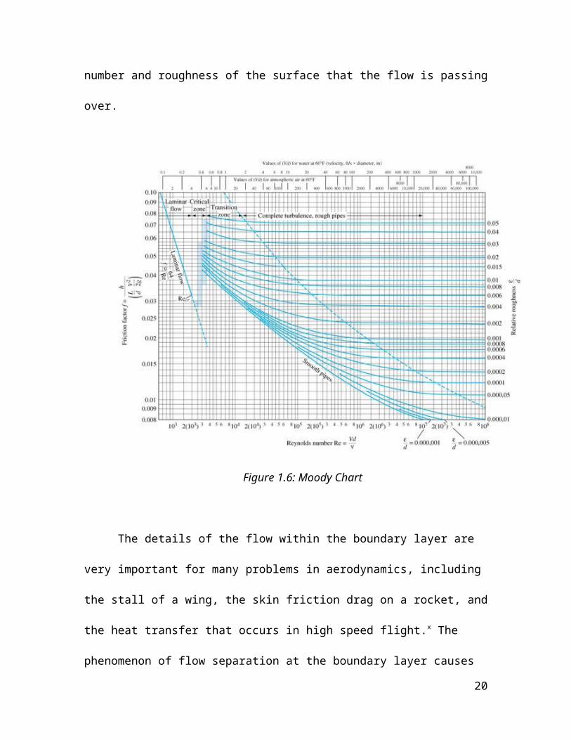
work in this transition range. Any Reynold’s number above the transition range indicates

fully turbulent flow, where streamline velocity is unsteady. The relationship between the

Reynold’s number and the flow can be seen in the Moody Chart below. It is worth noting

that the exact behavior of the boundary layer flow is a function of the Reynold’s number

and roughness of the surface that the flow is passing over.

13

Figure 1.6: Moody Chart

The details of the flow within the boundary layer are very important for many

problems in aerodynamics, including the stall of a wing, the skin friction drag on a

rocket, and the heat transfer that occurs in high speed flight.x The phenomenon of flow

separation at the boundary layer causes airplane wings to stall at high angles of attack.

Further study of the boundary layer shows that these effects create friction drag.

Frictional drag is associated with drag over blunt bodies and is described in greater detail

in the drag section. Figure 1.7 below shows the boundary layer effects on an airfoil. The

velocity profile becomes larger as airflow moves across the wing, starting from the

leading edge, and the flow changes from laminar to turbulent.

14

Figure 1.7 viii

Formation of Wakes

As was discussed briefly in the last section, there is a phenomenon where, as flow

passes over a bluff body, the boundary layer is observed to separate from the surface and

forms a wake behind the body. Visible wakes develop behind speeding boats in water.

Wakes also propagate behind airplane wings as a plane rolls down the runway for

takeoff. Again, various parameters determine whether or not the flow behavior before, at

the boundary layer, and in the wake are laminar or turbulent. Below is a depiction of a

wake forming behind a cylinder.

15

Figure 1.8: Turbulent Wake behind cylinder viii

In front of the cylinder exists a high-pressure stagnation point, and a low-pressure

wake forms behind the object as a result of the boundary layer separating the flow from

the object surface. Directly behind the bluff body, the static pressure drops but with a

distance of roughly 10 cylinder diameters behind the bluff body, the wake static pressure

returns to the static pressure as in the freestream flow. Additionally, a momentum

deficiency can be seen when examining the flow as a loss in velocity within the wake of

the bluff object. Mathematically, the deficiency is the difference in the mass flux from in

front to behind the body and can be determined using the equations for conservation of

mass and momentum.

As previously established, boundary layer separation is the main cause of the

wake behind the flow of a bluff body, and the behavior of the wake flow is heavily

determined by the Reynold’s number and roughness of the surface. Figure 1.9 below

shows how flows in the wake region can be laminar or turbulent depending on the

Reynold’s number, the location at which the boundary layer separates for each bluff

body, and where the effects of the fluid viscosity are important. Generally, as the

Reynold’s number is increased, the area of the wake of the cylinder where viscous effects

are important becomes smaller. It is known that shear stresses are produced as a result of

16

fluid viscosity and velocity gradient, so it makes sense that viscous effects are confined to

wake and boundary layer regions. xiii

Figure 1.9

Drag is an incredibly important area of study in fluids, mainly applied to

aerodynamics and study of flight. A bluff body in a flow usually experiences two

components of drag: frictional drag and pressure drag. Frictional drag stems from the

friction between the surface and flowing fluid over it. Frictional drag, as mentioned, is

related to the boundary layer and is heavily dependent upon Reynold’s number. Pressure

drag, related to a wake, is observed to be less sensitive to Reynold’s number. To further

compare, frictional drag is most important in flows where there is no boundary layer

17

separation and is related to surface area of the object in contact with the flow whereas

pressure drag is important in separated flows and is related to the cross-sectional area of

the body.xiv Interestingly enough, bodies that are dominated by frictional drag are

commonly called streamlined bodies, and bodies dominated by pressure drag are referred

to as bluff bodies. Figure 1.10 shows the difference in drag coefficients for streamlined

bodies, on the bottom, to bluff bodies on top. For thoroughness, in this lab, the flow

around both cylinders and airfoils were examined.

Figure 1.10 xiv

Drag is formally defined as a net force in the direction of flow due to the pressure

and shear forces on the surface of the object. Interestingly enough, most of the

information of drag on objects has been accumulated through numerous experiments with

18

wind tunnels, water tunnels, and other ingenious devices where drag can be measured on

scale models.xv The formulas used to quantitatively calculate friction and pressure drag

individually differ. Equation 9 below shows the generalized formula used to calculate

drag:

D= ρLu12∫

0

w

(1−u2

u1)dy

Equation 9

Where, D is the drag force, ρ is density of the fluid, u or (U) is the flow velocity,

and L is the chord length.

Directly proportional to drag is what is known as the coefficient of drag. This is a

dimensionless parameter that is a function of other dimensionless parameters, such as

Reynold’s number, Mach number, Froude number, and relative roughness of the object

surface. Again, refer to Figure 1.10 to observe the relation between coefficient of drag

and Reynold’s number for a cylinder and airfoil. For a given shape, the formula for the

coefficient of drag is defined below:

Cd=D

12

ρ U∞2 S

Equation 10

19

Where, Cd is the coefficient of drag, D is the drag force, ρ is density of the fluid,

u or (U) is the freestream, flow velocity, and S is the area of the contact surface.

To further relate the ideas of wake formation and drag on a bluff body, Figure

1.11 below shows the wake of a cylinder. The effects of drag on the velocity profile can

be seen from the change as the flow moves from left to right.

Figure 1.11 viii

Airfoil Theory

Study of flow around an airfoil is crucial in understanding the concepts of lift and

drag. An airfoil is simply in the shape of a wing or a blade, as can be seen in Figure 1.11,

and produces aerodynamic forces when within a flow.

20

Figure 1.11: Cross-section of airfoil viii

The three aerodynamic forces created as a result of flow are lift force, drag force, and

moment. The lift is a force that exists normal to the direction of the freestream velocity

and creates “lift” or upward movement. The drag force opposes freestream direction. The

pitching moment develops as a result of the magnitude and lines of action of the lift and

drag forces.

First, it is critical to understand how these forces relate back to fundamental

principles in fluids. As fluid flows over the unique shape of an airfoil, a boundary layer

forms on the surface. At an angle of attack of zero degrees, the boundary layer around a

symmetric airfoil is equal on both sides.viii If the airfoil has a non-zero angle of attack, a

different boundary layer forms on top than on the bottom. When analyzing the flow

outside the boundary layer, viscous effects can be disregarded, so Navier-Stokes

equations can be simplified to Bernoulli’s. Figure 1.12 below shows that velocity profile

over a non-symmetrical airfoil or with a nonzero angle of attack is greater on the top than

it is on the bottom.

21

Figure 1.12

In Bernoulli’s equation lies the proof that the velocity below the wing is lower than the

velocity of the fluid above the wing, so the pressure below the wing is higher than the

pressure above the wing. The effects of velocity on pressure in this case are

predominantly proportional to dynamic pressure in Bernoulli’s for flows with large

Reynold’s numbers. Thus, it is shown that the pressure below the wing is higher than the

pressure above the wing. This pressure difference induces lift on the wing, and, in the

case of an airplane, allows it to fly. xvi Below, Figure 1.13 shows the possible streamline

for Bernoulli analysis on the airfoil.

Figure 1.13

The pressure difference causes the net forces of drag and lift and, consequently,

moment as mentioned above. Drag in the case of an airfoil is different than that of a

cylinder because, as referenced above, an airfoil is not bluff but rather a streamlined

body. Even so, pressure drag is a major source of drag on the airfoil, resulting from the

component of pressure difference, which is parallel to the freestream. The pressure drag

22

exponentially increases as lift increases. As with a bluff body, the airfoil will cause a

momentum deficit in flow, but unlike a bluff body, the drag caused by this momentum

deficit is small compared to the pressure drag. The formulas for drag and drag coefficient

are in Equations 9 and 10 above.

Lift force and coefficient of lift are best categorized by the two equations below.

Equation 11 shows the dimensionless parameter for lift per unit area or coefficient of lift.

Equation 12 stems from the theory that the lift produced by a symmetric airfoil is directly

related to its angle of attack.

CL=L

12

ρU ∞2 S

Equation 11

CL=2 πα

Equation 12

In the 2 above equations CL is the coefficient of lift, ρ is density of the fluid, u or

(U) is the freestream flow velocity, and S is the area of the surface.

Figure 1.14 below shows the relation of lift and drag forces to angle of attack.

23

Figure 1.14

As angle of attack of the airfoil is increased, the boundary later stays attached to

the surface of the airfoil until a certain critical angle is reached. At this point, the

boundary later on the top of the airfoil begins to separate from the trailing edge of the

airfoil. If the angle gets too large, the boundary layer on the upper surface separates, the

flow over the wing develops a wide, turbulent wake region, the lift decreases, and drag

decreases creating a condition called a stall, also mentioned in the above section.xvii

Viscous effects and shear stresses contribute little to normal flow, but a stall is a special

condition where these play a role. In aircraft, stalling can be extremely detrimental to

flight and requires immediate action before the aircraft looses all lift.

24

Lastly, the forces produce a moment or “pitching” moment about the airfoil with

the coefficient of moment formula described below. At the leading edge of the airfoil, the

moment has a negative slope as lift increases. There is a point on the airfoil where the

moment is zero, regardless of the magnitude of lift. This point is considered the mean

aerodynamic center.viii

CM= M12

ρ U∞2 Sx

Equation 13

Where M is the moment, ρ is density of the fluid, u or (U) is the freestream flow

velocity, x is chord length, and S is the area of the surface.

This pitching moment only occurs when an aerodynamic force, such as those

discussed above, is applied at the aerodynamic center of the airfoil. The aerodynamic

center is not quite the center of pressure on the airfoil but rather a point for which the

coefficient of the pitching moment remains nearly constant regardless of angle of attack.

2-D v. 3-D Objects

From what has been discussed about flow and drag, it is apparent that behavior of

flow is heavily dependent on the surface features of the object in contact with it. In the

wind tunnel test section of this experiment, the object in the flow could be considered

either two or three-dimensional.viii If the object spans the entire test section, the object is

considered to have infinite span from the perspective of the incoming flow. The flow

does not wrap around the edges of the object but only passes from above and below.

25

Therefore, the object is approximated as two-dimensional. An object that does not span

the entire width of the test section is considered three-dimensional

Figure 1.15: Two-dimensional body (left), three-dimensional body (right)

An object in two-dimensional flow has less drag than one in three-dimensional

flow. This is because a three-dimensional object has boundary layer separation on the

top, bottom, and sides, whereas a two-dimensional object would only experience that

separation on the top and on the bottom. As evidenced by Equation 10 for coefficient of

drag, the increased boundary layer separation and surface area will lead to increased

pressure drag. Lastly, additional energy in lost at the tips of the three-dimensional object

because of trailing vortices.viii

Von Karman Vortex Shedding – Unsteady Aerodynamics

Up until now, most topics discussed in this introduction have been explained in

terms of steady, inviscid, and irrotational flow behavior. These assumptions allow for the

26

Navier-Stokes equations to be simplified into Bernoulli’s. In reality, even everyday

phenomena are far more complicated to explain.

A Von Karman vortex street is a repeating pattern of swirling vortices caused by

unsteady separation of flow over bluff bodies.viii Depending on the Reynold’s number and

body parameters of the object, vortices can be continuously shed off the edges of the

body. Eventually, viscosity of the flow or fluid will drain the energy of the vortices and

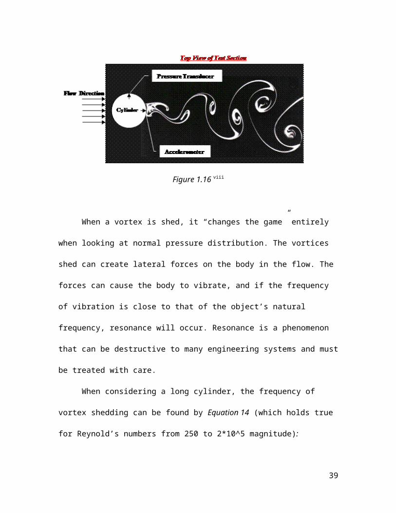
cause them to die down with distance. Figure 1.16 below shows vortex shedding around

a cylinder.

Figure 1.16 viii

When a vortex is shed, it “changes the game” entirely when looking at normal

pressure distribution. The vortices shed can create lateral forces on the body in the flow.

The forces can cause the body to vibrate, and if the frequency of vibration is close to that

of the object’s natural frequency, resonance will occur. Resonance is a phenomenon that

can be destructive to many engineering systems and must be treated with care.

27

When considering a long cylinder, the frequency of vortex shedding can be found

by Equation 14 (which holds true for Reynold’s numbers from 250 to 2*10^5

magnitude):

f ∗dU∞

=0.198(1−19.7ℜ )

Equation 14

The dimensionless parameter to the left ( f ∗dU ∞

) is known as the Strouhal number.

This is a measure of the ratio of inertial forces due to unsteadiness of the flow to inertial

changes due to changes in velocity from point to point in the flow field.

28

III. Procedure

The following procedure for this lab was split over the course of two weeks. All

parts were performed by a group of about 10 engineering students.

Week 1

Equipment

Closed loop wind tunnel

Pitot-static tube

Aerolab Pyramidal Force Balance

o 3 load cells

NACA 0012 airfoil

Daytronic System 10 DataPac

Pressure Systems 9010 Optomux

3x 2” O.D. Cylinder

Pitot tube rake

Thermometer

Labview

Part 1: Force Balance and Calibration

1. Calibrating Lift

a. The carriage chord was run through three pulleys and connected to the

middle hole on the force balance.

b. A starting 5-pound weight was put on the carriage.

c. Labview was run to collect lift data from the weight.

29

d. The carriage weight was increased by 5 pound increments each trial.

e. Labview was run to collect data from each trial.

f. The trials continued until a carriage weight of 25 pounds was reached.

g. All measurements were saved and the weights were unloaded from the

carriage.

1. Calibrating Drag

a. A new Labview file was opened.

b. The carriage chord was removed from the middle hole and run through the

end hole on the force balance.

c. The 5-pound weight was loaded onto the carriage.

d. Labview was run to collect the drag data.

e. The carriage weight was increased from 5 pounds to 25 pounds in 5-pound

increments.

f. Labview was run to collect calibration data from each trial until 25 pounds

was reached.

2. Calibrating Moment

a. A new Labview file was opened.

b. The carriage, along with weights, was removed and placed aside.

c. A one-pound weight attached to string was strung around the first notch of

the top metal cylinder.

d. The distance was measured outward from the center of the cylinder.

e. Labview was run to collect the data.

30

f. The weight was moved to the next notch and the distance from the center

of the cylinder was noted.

g. Steps d-f were repeated until the last notch on the opposite side was

reached.

 Part 2: Boundary Layer

The wind tunnel was run at 15 Hz for Part 2.

1. The access window to the wind tunnel was opened.

2. A pitot-static tube was placed in the first hole in the middle of the test section,

approximately 30 cm from the wall.

3. The pitot-static tube was aligned parallel to the freestream flow.

4. The pitot-static tube was moved toward the floor in 5 cm increments.

5. When the pitot static tube reached 5 cm off the wall, it was then moved toward

the floor in 0.5 cm increments.

6. The pressure was measured at each location and temperature was noted. (total of

10 times)

7. The pitot-static tube was moved to the second hole downstream and steps 3-6

were repeated with the tube in it’s new location.

Part 3: Wake

1. Wind tunnel was opened

2. The distance between each tap on the rake was measured.

3. The rake was the placed inside the wind tunnel, initially without the presence of

the cylinder.

31

4. Wind tunnel was turned on and run at 25 Hz.

5. Labview was run 20 times. With each time, pressure measurements were read and

recorded.

6. Cylinder was then mounted 6 diameters ahead of the rake in the wind tunnel.

7. The wind tunnel was then turned on and run again with the cylinder.

8. Labview was run again to record pressure data in a new file. (20 times to get the

average)

Week 2

Equipment

Closed loop wind tunnel

Pitot-static tube

Aerolab Pyramidal Force Balance

o 3 load cells

NACA 0012 airfoil

Daytronic System 10 DataPac

Pressure Systems 9010 Optomux

5x 4.8cm O.D. Cylinder

o Lengths: 10.5”, 18”, 20”, 22”, and 24” (convert to SI units)

Pitot tube rake

Thermometer

Labview 6i

Accelerometer

32

2x High Frequency Pressure Transducer

Part 1: Freestream Velocity

1. Pitot tube was placed upstream of the model. The angle of the pitot tube was

adjusted to be parallel to the freestream flow to achieve maximum dynamic

pressure.

2. Dynamic pressure was recorded 20 times for the average

Part 2: Airfoil

1. Airfoil was placed on top of the force balance in the wind tunnel.

2. The wind tunnel was turned on running at 30 Hz.

3. The angle of the airfoil was adjusted until the lift was equal to zero. In other

words, the degree of attack was zero.

4. Airfoil angle was then adjusted to -6 degrees. From here, lift, drag, and pitching

moment data were recorded via Labview.

5. The angle of attack was then increased by 2 degrees. (20 increments on the dial)

6. This was repeated until an angle of attack of 18 degrees was reached.

7. Wind tunnel speed was increased to 45 Hz (with a new Labview file)

8. Steps 4-6 were repeated.

9. The airfoil chord length and depth were measured.

Part 3: Cylinders

1. 20 measurements of dynamic pressure of upstream model were taken.

2. The length and outside diameter of each of the three cylinders were measured.

33

3. The first cylinder, labeled number 1, was inserted into the wind tunnel.

4. The cylinder was placed perpendicular to the flow.

5. Wind tunnel was turned on at 30 Hz.

6. The drag produced from the cylinder was measured and recorded via LabView.

7. Steps 4-6 were repeated for each cylinder and mount alone, using new LabView

files for each.

Part 4: Vortex Shedding

1. The length and diameter of the cylinder were measured.

2. 24” long cylinder with accelerometer was secured into the first hole in the bottom

of the test section.

3. Wind tunnel speed was turned on to 35 Hz.

4. The dynamic pressure was measured 20 times to obtain the average.

5. The sampling frequency was set to 7500 Hz and 10240 sample time.

6. Accelerometer data was collected via LabView.

7. The wind tunnel speed was then increased to 40 Hz.

8. Steps 4-6 were repeated.

9. The old cylinder was removed and a cylinder with pressure transducers was now

placed in the wind tunnel.

10. The dynamic pressure was measured, again, 20 times.

11. Pressure data was recorded for several seconds.

34

IV. Results and Discussion

Given the wide range of topics encompassed by this study, both theoretical and

practical, the lab work was split up into two weeks. During the first week, work was done

on force balance and calibration, experiments with the pitot-static tube, observing

boundary layers, and wakes caused by flow around cylinders. The second week included

studying flow around an airfoil, vortex shedding, and flows around 2-D and 3-D objects.

The results of each of these trials are published and discussed below. All data presented is

in SI units.

Week 1

Part 1: Force Balance and Calibration

This part was in essence the simplest part of the lab to collect data from, yet very

important. A force balance with attached to known weights was used to calibrate the load

cells in the sensors. As discussed in the introduction, this was done to prevent “drift” and

to ensure that the integrity of the results obtained further in this lab not be compromised

by error due to drift.

Using the force balance, Labview, and the setup described in the procedure,

results were calibrated for lift force, drag, force and moment. Figure 1.1.1 in this section

shows each plot where lift, drag, and moment are respectively are plotted against the

voltage readings from the load cells. It stands to reason that when no weight is applied,

there should be no force reading.

The drift for the moment data was the farther than the drift seen in the lift and

drag data. A line of best fit was taken through the data points and the y-intercept was

35

recorded for each. The data was linear, as expected, therefore each line of best fit was in

the format of y=m*x+b. All data was effectively “zeroed” using the y-intercept

information for lift, drag, and moment.

Figure 1.1.1

36

Part 2: Boundary Layer Test

The wind tunnel and a pitot-static tube were used to emulate boundary layer

flow conditions in this section. The wind tunnel was run at a speed of 15 Hz, once

with the pitot-static tube in a location upstream relative to the flow and another

where the tube was downstream. At each location, the tube was first placed about

25 cm above the ground, and then lowered incrementally, and the wind tunnel was

run each time the tube was lowered. At every height, the tube collected pressure

readings which were taken and converted into velocities using Bernoulli’s

equations. Moving the tube closer and closer to the flat surface of the wind tunnel

showed the change in the velocity profile of the fluid near the boundary layer of the

flow. Figure 1.2.1 has the results of both the upstream and downstream velocity

data.

37

Figure 1.2.1

The results of Figure 1.2.1 show the upstream and downstream trends in velocity

from a tube height of about 25 cm above the ground to about 0 cm. The data obtained is

in accordance with the boundary layer theory discussed in the introduction. Starting with

the similarities, the freestream flow velocity of both profiles remained consistent for a

tube height of about 1 to 25 cm with upstream flow at around 12.6 m/s and downstream

flow at about 13.7 m/s. The flow down the center of the wind tunnel notably displays

steady-state qualities. Observing the upstream profile, at about 0.5 cm from the flat

surface, there was a drop in velocity. Velocity continued to decrease in large increments,

indicating that the flow was experiencing the viscous effects of the boundary layer. The

38

same velocity drop happened with the downstream velocity profile at around a height of 1

cm off the wind tunnel floor.

At a small distance off the ground, both of the flows began experiencing viscous

effects and exhibiting turbulent behavior. The drop off in velocity confirms that the flows

encountered the “no-slip” condition when at the boundary layer.

The relatively quick drop in velocity over a small distance in the upstream profile

demonstrated how thin the boundary layer was. The downstream velocity profile

experienced a slower decrease at a greater height from the surface. This indicates that the

boundary layer downstream was thicker than the one upstream. This reinforces the theory

behind boundary layers: fluid viscosity and turbulent behavior had a slightly greater

effect downstream than the effect seen upstream.

Part 3: Wake Test

In this section, a cylinder was placed in the wind tunnel to examine the effect

a bluff body would have on a flow. This portion was run twice: once at 30 Hz and

once at 45 Hz. For each speed, the tunnel was run once without the cylinder to

obtain the accurate freestream velocity of the flow at every other tap in the rake

tube. Figure 1.3.1 below shows the velocity data collected at 30 and 45 Hz, both with

and without the presence of the cylinder. Table 1.3.1 has the quantitative results for

this section.

39

Figure 1.3.1

The flow without the cylinder was consistent for the most part as expected. The

spike in the blue lines in Figure 1.3.1 must be attributed to error. It is possible that one of

the taps on the rake tube was bent or not reading accurately. Nevertheless, the flow acted

as expected with the presence of the cylinder.

The flow passing at the far ends of the cylinder hitting the first and last pins on

the rake tube had the same velocity as the freestream. Since the cylinder spanned the

entire width of the test section, it is considered a two-dimensional flow. Moving more

towards the center, there was a noticeable decrease in velocity. This is in accordance with

the theory discussed above: the flow hitting the front of the cylinder creates a stagnation

40

point. The wake directly behind that point contains turbulent fluid motion. As a result of

more fluid particles colliding in turbulent flow, velocity is decreased.

Using the given parameters for this section, the drag and coefficient of drag were

calculated along with the momentum deficit and Reynold’s numbers. As discussed in the

introduction, the presence of a bluff body, such as a cylinder, produces a momentum

deficit. The results were exactly as expected with the momentum deficit calculated as the

area between the two curves. The drag force and coefficient of drag were calculated using

the Equations 9 and 10 in the introduction, and the numbers made sense given the

freestream velocity.

Table 1.3.1

30 Hz 45 Hz

Momentum Deficit 17.747 28.165

Drag Force (N) 40.916 ± 4.93 98.043 ± 12.44

Coefficient of Drag 1.45 ± 0.18 1.49 ± 0.18

Reynold’s Number 1.074*10^5 ± 2.70*10^3 1.644*10^5 ± 4.18*10^3

41

Week 2

Part 1: Airfoil Test

The purpose of this section was to examine properties of a flow over an airfoil.

The angle of attack of the airfoil was changed from -6 to 18 degrees in 2-degree

increments. The data was taken at 30 Hz and again at 45 Hz. Lift, drag, moment and

their corresponding coefficients were calculated and analyzed in this section.

Strings were attached to the front of the airfoil to indicate stalling or to help

visualize when the boundary layer begins to separate from the airfoil.

Figure 2.1.2

42

From the above graphs, it is easy the see the trends between each coefficient and

the angle of attack. The coefficient of lift was observed to increase with increasing angle

of attack. At about 17 degrees, the plot shows the coefficient of lift drops and then levels

out, indicating a stall. At this same angle, the drag force on the airfoil increased. This is

the point where the tufts (strings) visibly separated from the airfoil. At this point, viscous

effects became prevalent as the boundary layer further separated from the airfoil. The

logistics of a stall are discussed more in depth in the introduction.

Table 2.1.1

30 Hz 45 Hz

Slope of coefficient of lift v. angle of attack

1.604 1.679

Reynold’s Number 3.00*10^5 ± 3.113*10^4 4.469*10^5 ± 4.634*10^4

Table 2.1.1 displays some of the quantitative data collected in this section. The

ideal or theoretical value for the slope of the coefficient of lift v. angle of attack is about

6.28. The results obtained in this section do not match up exactly with the ideal number.

Some of this discrepancy could be attributed to error in conducting the experiment or in

the collection of the data. The main difference is that the airfoil that was used during this

section was not “thin” and therefore would not produce the same amount of lift as the

airfoil being considered in the theoretical calculation. The slope values and Reynold’s

numbers along with the graphs obtained from this section do in fact confirm the

theoretical fluid principles concerning airfoils.

43

The Reynold’s number directly affects the coefficients of drag and lift, as

discussed in detail in the introduction. With decreasing Reynold’s number drag increases

and lift decreases. The results obtained in this section are in accordance with this theory.

Part 2: Cylinder Drag Test

Different cylinders were used in this portion of the experiment to examine

how aspects of drag changed with varying lengths. Table 2.2.1 below shows the

coefficients of drag and Reynold’s numbers measured for each cylinder. Differences

were also examined in the flow with both two-dimensional flow and three-

dimensional flow occurring for different cylinder lengths.

Table 2.2.1

Cylinder 1 Cylinder 2 Cylinder 3 Cylinder 4 Cylinder 5

Length (m) 0.603 0.559 0.508 0.457 0.267

Coefficient of Drag

0.7035 ± 0.0871

0.6344 ± 0.0785

0.6070 ± 0.0751

0.6150 ± 0.0761

0.5205 ± 0.0644

Reynold’s Number

9.971*10^4 ±1.2*10^4

9.975*10^4 ±1.2*10^4

9.978*10^4 ±1.2*10^4

9.982*10^4 ±1.2*10^4

9.986*10^4 ±1.2*10^4

Though the lengths do not differ much, there is still a noticeable change in each

drag coefficient. As cylinder length decreases, the coefficients of drag also decrease.

Considering the formula for drag, area (or characteristic length) directly factors in. It

makes sense that the Cylinder 5, the one with the least area in contact with the flow, has

the lowest coefficient of drag. Since the Reynold’s number is inversely proportional to

the coefficient of drag, it increases as coefficient of drag decrease. All of the empirical

44

results found here validate the preexisting theory. Comparison with other data found on

the web further validates these results.

The cylinder that was used in the wake test spanned the length of the entire test

section and, therefore, was characterized as two-dimensional flow. The cylinders used in

this section did not span the length of the test section. In addition to going above and

below the cylinders, the airflow also passed from the sides. As a result, the cylinders in

the three-dimensional flow experienced more drag.

Part 3: Vortex Shedding

The final part of this two-week experiment was done for the purpose of

generating and observing unsteady flow. This section was run twice: once at 35 Hz

and a second time at 40 Hz. Data was collected for both runs off of a pressure

transducer and an accelerometer. The results in Table 2.3.1 below shows all of the

quantitative data collected in this section.

Table 2.3.1

45

Vortex shedding frequency was calculated twice: once with the use of the

empirical formula given in the introduction and once by using the maximum point on the

frequency domain plots shown below. A fast Fourier transform was used to take the plots

from the accelerometer and pressure transducer data and converted them to the frequency

domain. The measured values from the accelerometer and transducer data were relatively

similar for each given run. The empirical results were off by a small factor. The

discrepancy in these values could be attributed to uncertainty in measurement.

Looking at Figures 2.3.1. and 2.3.2 below, the accelerometer data indicates that

the cylinder vibrated most violently at a wind tunnel speed of 35 Hz. The noise from the

time domain data had greater amplitude in the 35 Hz run than the 40 Hz trial. The

frequency domain data also pointed to a larger spike in the 35 Hz run. The magnitude of

the vibrations were most likely caused by how close the vortex shedding frequency was

to the cylinder’s natural frequency. In other words, the most violent vibrations did not

occur at the faster wind speed because, even though velocity was greater, the vibrations

46

from the vortices were at a frequency farther from the cylinder’s natural frequency. This

is in accordance with the theory discussed in the introduction: if the frequencies produced

by vortex shedding are close to the natural frequencies of the object in the flow, the

object can reach resonance.

Vortex shedding frequency can be deduced using empirical methods, pressure

data, and accelerometer data. The accelerometer data provides the most direct

experimental way to find frequency. Using Fourier analysis, data in the pressure data in

the time domain can be converted into frequency data. Empirically, vortex-shedding

frequency is related to freestream velocity and Reynold’s number of a flow. The results

of this last section are all in accordance with fluid theory.

47

Figure 2.3.1

Figure 2.3.2

48

Figure 2.3.3

Figure 2.3.4

49

V. Conclusion

The work done in this lab merely scratched the surface of the complex and

intricate field of fluid mechanics. The simple ideas explored here develop into profound

applications of fluids in engineering. The first portion of the lab demonstrated how

important calibration was to lessen error in calculation. The boundary layer portion of

this test was relatively simple to conduct but has profound theory backing the actual

experiment. Parameters such as the Reynold’s and Strouhal numbers play a vital role in

flow. Laminar and turbulent flow were first introduced when examining boundary layer

separation. The concepts governing boundary layer separation were directly related to

studying the behavior of wakes. Understanding how an object in a flow creates drag

force, lift force, moments, and their respective coefficients was undoubtedly one of the

most important lessons to be learned. That understanding was then used to analyze flow

around an airfoil. Studying the airfoil alone and how angle of attack affected the forces

present as a result of airflow led to a slightly better understanding of how immensely

large objects such as planes can lift off the ground. Vortex shedding was the last thing

examined in this lab because it involved an examination of unsteady flow: notably a

difficult area to understand even in the field of fluids.

Fluid mechanics is a discipline based on both complex physical laws and

seemingly impossible math. The subject incorporates an endless number of theories and

ideas that are interrelated to analyze flows. The intricacy of flows go well and beyond the

scope of what was examined in this lab. All else aside, without knowledge and

application of fluid mechanics, many of the engineering marvels in the world today

simply would not exist.

50

VI. References

51

i http://www.scienceclarified.com/everyday/Real-Life-Chemistry-Vol-3-Physics-Vol-1/Fluid-Mechanics.htmliiFundamentals of Fluid Mechanics, 6th Edition, By Munson, Young, Okiishi, Heubsh

iii Fundamentals of Fluid Mechanics, 6th Edition, By Munson, Young, Okiishi, Heubshiv http://www.efm.leeds.ac.uk/CIVE/CIVE1400/Section1/Fluid_properties.htmvFundamentals of Fluid Mechanics, 6th Edition, By Munson, Young, Okiishi, … p. 152vihttp://www.coilgun.eclipse.co.uk/images/theory_pages_images/general_diagrams/form_drag_streamlines_2.gifvii http://en.citizendium.org/wiki/Fluid_dynamicsviii http://lcs3.syr.edu/faculty/glauser/MAE315/Fluids/MAE315Lab4Week1.htmix Fundamentals of Fluid Mechanics, 6th Edition, By Munson, Young, Okiishi, … p.308x http://exploration.grc.nasa.gov/education/rocket/boundlay.htmlxi http://output.to/sideway/images/fluid_viscosity.jpgxii http://blog.nialbarker.com/wp-content/uploads/2010/03/laminar_turbulent_flow.gifxiii Fundamentals of Fluid Mechanics, 6th Edition, By Munson, Young, Okiishi, … p. 469xiv http://www.princeton.edu/~asmits/Bicycle_web/blunt.htmlxv Fundamentals of Fluid Mechanics, 6th Edition, By Munson, Young, Okiishi, … p. 493xvi http://web.mit.edu/2.972/www/reports/airfoil/airfoil.htmlxvii Fundamentals of Fluid Mechanics, 6th Edition, By Munson, Young, Okiishi, … p. 515