1 of 4

Introduction to Economic Growth Development of Modern Growth Theory Questions -

1. Why are some people (countries) rich and some poor? Need to find determinants of GDP and growth rates to answer this

2. Why do some countries grow faster than others? 3. In long-run, is growth rate exogenous or endogenous?

Endogenous Variable - Determined by decisions (usually based on optimizing behavior; e.g., maximize utility leads to demand; maximize profit leads to supply); (2) something you can change through policy (e.g., tax will change PD, PS, and Q) Supply & Demand - PD = a - bQ and PS = c + dQ; this leads to PD = PS = a - bQ = c + dQ

� Q = (a - c)/(d + b) ∴ Q is given (endogenous) Growth Rate - can policies affect growth rate (i.e., is growth rate endogenous)?

neoclassical theory says yes, but only in transition, not in long-run; some newer theories say yes; others say no

Technology - technical description: production function; intuitive: instructions for how to produce things Rice Example - cooking rice requires a pot and heat source (capital), rice and water

(resources), and a recipe with directions on how to cook it (technology) Steady State Equilibrium - also called long-run equilibrium; all variables grow at a constant

rates (could be different from each other, but constant over [or independent of] time) Brief History -

Adam Smith - focused on accumulation of capital Carl Marx - focused on technological change and unemployment Ricardo - focused on class structure Neoclassical Growth Theory - Solow (1956); assumptions:

• Perfect competition in all markets • Exogenous rate of population growth (in long-run) • Exogenous rate of technological change (in long-run) • Endogenous income per capita levels • Endogenous transitional growth rates

Example - look at income per capita (y); we can change the growth rate (dy/dT) in transition, but not in the long-run (i.e., slope stays the same)

New Growth Theory - Romer (1986) & Lucas (1988); also called endogenous growth theory because now long-run growth rate can change; dropped perfect competition assumption and made technical change endogenous

Schumpeterian Approach to Economic Growth - new products have short lifetimes (all companies from the original Dow Industrial list are gone except General Electric); firms enjoy temporary monopoly power (imperfect competition) then are replaced (creative destruction); all used fixed population (not realistic) because introducing any population growth means economic growth unlimited (also not realistic) Grossman & Hylpman (1991), Aghion & Howitt (1992), Segerstrom, et. al. (1990) -

focused on product quality Romer (1990) - focused on product variety

Time

Time

y

dy/dT

y is higher than it would've been, but still grows at same rate

2 of 4

Schumpeterian Without Scale Effects - original Schumpeterian approach had scale effects which made growth rate change with population rate (e.g., double population caused growth to double); modification without scale effects fixed the problem Jones (1995); Segerstrom (1990) - exogenous long-run growth Howitt (1999); Dinopoulos & Thompson (1999) - endogenous long-run growth

Facts on Economic Growth 1. There is enormous variation in per capita

income across economies. The poorest counties have per capita incomes that are less then 5 percent of per capita incomes in the richest countries

GDP - gross domestic product; monetary value of all goods and services produced within a nation's borders in 1 year; doesn't matter which company does it (e.g., Honda Accords built in Ohio count towards US GDP)

GNP - gross national product; similar to GDP except it's goods and services produces by a nation's companies (e.g., Honda Accords built in Ohio count towards Japan's GNP) Difference - GDP better to use because

it reflects quality of life more than GNP, but in long-run both are very similar

Purchasing Power Parity - used to develop exchange rates for GDP comparisons; attempts to measure actual value of a currency in terms of its ability to purchase similar products (e.g., Big Mac in U.S. costs $2 and in Japan costs 300 yen � PPP exchange rate is 150 yen/$)

Per Capita Income - GDP per person; useful "summary statistic" of the level of economic development because it's highly correlated with other measures of quality of life

GDP Per Worker - tells more about productivity of the labor force (whereas GDP per person is general measure of welfare)

Why is there a difference?

"Fair"

Lots of poor

3 of 4

2. Rates of economic growth vary substantially across countries. Growth - the amount by which something changes (first derivative) Growth Rate - amount by which something changes divided by initial value (first

derivative over variable) Constant Growth Rate - measure of interest grows exponentially at a constant rate;

graph looks exponential, but on a ln scale it's linear with slope equal to the growth rate Example - L(t) = labor force at time t; labor growth = L'(t); labor growth rate = n; we

can relate these by definition: L'(t)/L(t) = n Now solve for L(t) by writing out L'(t) as dL/dt: dL/dt/L(t) = n

Move dt to right side and integrate: �� = ndttLdL )(/

Work out integrals: ln L(t) = nt + c (constant) Use exponential: eln L(t) = L(t) = ent + c = ecent Notice that using t = 0, means that L(0) = ec Rewrite L(0) as L0 and we solved for L(t) in terms of L0 and growth rate n:

L(t) = L0ent

(This is general equation for any constant growth rate) Going the other way - differentiate to find L'(t) = L0e

nt⋅d(nt)/dt = nL0ent

Use growth rate definition: L'(t)/L(t) = nL0ent/L0e

nt = n Yet another way - take ln of both sides: ln L(t) = ln L0 + nt (used for regression)

Now take derivative of both sides wrt t: ∂ln L(t)/∂t = ∂ln L0/∂t + ∂nt/∂t L'(t)/L(t) = 0 + n = n

Years to Double - useful way to interpret growth rates introduced by Robert Lucas ("On the Mechanics of Economic Development," 1988); solve for t in order to double income Y(t) from Y0: 2Y0 = Y0e

gt � 2 = egt Take ln of both sides: ln 2 = gt

Solve for t: t = ln 2/g ≅≅≅≅ 0.7/g

∴ country growing at g percent per year will double per capita income every 70/g

3. Growth rates are not generally constant over time. For the world as a whole, growth rates were close to zero over most of history but have increased sharply in the twentieth century. For individual countries, growth rates also change over time.

Note: some growth models don't allow growth rate to change in long-run, just in transition

Dismal Science - prior to higher rates of growth, Thomas Malthus argued that population growth was exponential, but food production was linear; he argued that we would have endless wars to control population growth (coined term "dismal science" for economics)

4. A country's relative position in the world distribution of per capital incomes is not

immutable. Countries can move from being "poor" to being "rich," and vice-versa.

L(t)

Slope = n

t

L0

ln L(t)

t

ln L0

4 of 4

5. In the United States (general for most economics "in the long run") over the last century, a. rate of return to capital, r, shows no trend upward or downward

r constant (≅ 3%) based on interest rate on government debt

b. shares of income devoted to capital, rK/Y, and labor, wL/Y, show no trend

Labor constant (≅ 70% GDP � capital ≅ 30% GDP); also, labor 50-50 between skilled and unskilled

c. average growth rate of output per person has been positive and relatively constant over time; i.e., the United States exhibits steady, sustained per capita income growth

g constant (≅ 1.8%) 6. Growth in output and growth in the volume of international trade are closely related. Strong

positive correlation between international trade and growth (i.e., nations that trade more have higher GDP)

Volume of Trade - sum of exports and imports

1 of 7

Neoclassical Growth Models Model - mathematical representation of some aspect of the economy; best models are often

very simple but convey enormous insight into how the world works "All theory depends on assumptions which are not quite true. That is what makes it theory. The

art of successful theorizing is to make the inevitable simplifying assumptions in such a way that the final results are not very sensitive." - Robert Solow, 1956

Solow Model Assumptions

1. Single, homogeneous good (output) - this also implies that there is no international trade (have to have at least two different goods for any trade to take place)

2. Technology is exogenous - technology available to firms is unaffected by the actions of the firms, including R&D (we'll relax this later); implication is that production function is not shifting

3. Keynesian Assumption - individuals save a constant fraction of their income (i.e., people consume in proportion to income)... this assumption is consistent with the data... let the savings rate be s ∴ total savings is sY

4. Labor Force - population is same as labor force (good enough to have constant labor force participation rate); population grows at constant rate n ∴ L(t) = L0e

nt 5. Perfect Competition - zero economic profit; price takers in labor market (w) and capital

market (r) 6. Constant Returns to Scale - can use any constant returns production function (i.e.,

double input produces double output); we'll focus on Cobb-Douglas Two Inputs - capital and labor; capital is accumulated endogenously through

savings Constant Elasticity of Substitution (CS) - production function with constant returns

to scale; generalization of Cobb-Douglas; Y(t) = F(K,L) = [bKρ + cLρ]1/ρ Cobb-Douglas Function - Y(t) = F(K,L) = KαL1-α, α ∈ (0,1)

Test Constant Returns - F(2K,2L) = (2K)α(2L)1-α = 2KαL1-α = 2F(K,L)... yep 7. Constant Depreciation Rate - capital depreciates at a constant rate δ

Basic Model - built around two equations: production function & capital accumulation equation

I. Production Function - describes how capital inputs, K(t), combine with labor, L(t), to produce output, Y(t) Capital - look at corn... some you eat (consumption), some you plant to eat more in the

future (capital); capital postpones consumption by certain amount in hopes of higher (but uncertain) future consumption... definition of investment

Max Profits - hire capital and labor at market prices to maximize profits (Note: we can consider our good to be a numeraire (P = 1) which means r and w are in terms of Y) Max F(K,L) - rK - wL

First Order Conditions -

0=−= rFdK

dK

π... marginal product of capital = r

2 of 7

0=−= wFdL

dL

π... marginal product of labor = w

Using Cobb-Douglas -

rLKFK == −− ααα 11 � K

Y

K

LKr

αα αα

==−1

wLKFL =−= −− 1)1()1( ααα � L

Y

L

LKw

)1()1( 1 αα αα −=−=−

... we can use this

to get the demand for labor Finding Steady State - in order to find some form of the production function to give us a

steady state, we need to identify variables that won't change over time; in this case, we can focus on r & w because (1) empirical data says they're stable over time [fact 5 from Introduction to Growth], (2) based on the way the production function is set up, if either of these variables grows, the other has to decline and if we're talking growth rates, that means the other variable will eventually reach zero... not realistic

From first order conditions we have L

Yw

)1( α−= ∴ L

Y is also constant; that's called

the output per worker : L

Yy ≡

We also have K

Yr

α= ∴ K

Y is also constant; to put things in same terms (per

worker or per capita), we'll use a trick: k

y

LK

LY =/

/; since y is constant that

means capital per worker : L

Kk ≡ is also constant

Results for Production Function - 1. Zero Profit - results from constant returns assumption;

Profit = 0)1()1( =−−−=−−−=−− YYY

L

YK

K

YYwLrKY αααα

∴ payments to inputs completely exhaust the value of output produced 2. Constant Labor & Capital - as fractions of GDP; results from Cobb-Douglas

production function: α=Y

rK and α−= 1

Y

wL; this agrees with empirical data

(see fact 5 from Introduction to Growth) 3. Growth Rates Equal - take ln of both sides of capital per worker: k = K/L

LKk lnlnln −=

Totally differentiate wrt t: dt

dL

Ldt

dK

Kdt

dk

k

111 −= or L

L

K

K

k

k ���

−=

Those are growth rates; k is a stable variable in steady state so dk/dt = 0; that

means L

L

K

K ��

= ... the growth rate of capital equals the growth rate of labor

in the steady state

3 of 7

Per Capita Production - now that we have steady state variables we can work with (k and y), we need to convert the production function to incorporate these variables:

),( LKFY = ... because of constant returns to scale, we can write

)1,(, kFL

L

L

KF

L

Yy =�

�

���

�== ... introduce per capita production function f : )(kfy =

Using Cobb-Douglas - αα

αααα

kL

KLK

L

LKkfy =�

�

���

�==== −−1

)(

0' 1 >= −ααky ∴ output per worker always increases with k increases

0)1('' 2 <−= −ααα ky (because α < 1) ∴ we have diminishing returns to capital (the added output per worker by increasing capital per worker declines as we add more capital)

II. Capital Accumulation - the change in the capital stock over time is equal to the infusion of new capital from savings (sY) minus the depreciation of capital

KsYKdt

dK δ−== �

Example - economy starts with output of 100 and capital base of 200; the capital depreciate rate is 5 percent and the savings rate is 30 percent Savings (gross investment) = sY = 0.3(100) = 30 Depreciation = δK = 0.05(200) = 10 Capital accumulation (net investment) = sY - δK = 30 - 10 = 20

Per Capita Capital Accumulation - just like we did with the production function, we want to get this equation to incorporate variables that are constant in the steady state (k and y)

Divide all terms by K: δδ −=−=K

Ys

K

K

K

Ys

K

dtdK /

Where did we see that K

dtdK / term before? We got it from differentiation

LKk lnlnln −= wrt t when we showed that the growth rates of capital and labor are equal in the steady state (on previous page); the general (non steady state)

result was L

dtdL

K

dtdK

k

dtdk /// −=

From assumption 4 substitute the labor growth rate n: nK

dtdK

k

dtdk −= //

Solve that for K

dtdK /: n

k

dtdk

K

dtdK += //

Substitute that into the first equation we had: δ−=+K

Ysn

k

dtdk /

To get y into the equation, use the L/L trick again: δδ −=−=+k

ys

LK

LYsn

k

dtdk

/

//

Solve for capital accumulation per worker: knsydt

dk)( δ+−=

Steady State - in steady state, k must be constant so dk/dt = 0 � knsy )( δ+=

k

y

y = f(k) = kα

4 of 7

That is, the gross savings (investment in capital) per worker must equal the lost capital per worker (lost through depreciation and the increase in the number of workers)

Solve for Growth Rates - use formulas with standard trick of taking ln of both sides, then differentiating

αky = � ky lnln α= � k

k

y

y �� α= ... since 0=k� , we must have 0=y�

αα −= 1LKY � LKY ln)1(lnln αα −+= � =−+=L

L

K

K

Y

Y ���

)1( αα

nnn =−+ )1( αα ... so output grows at same rate as labor force Graphically - the Solow model is pretty easy to solve graphically... just

look at where sy intersects (δ + n)k Stable Equilibrium - if we have k anywhere other than k*, it'll

eventually adjust to be at k*; for example, start with k < k*; this means savings outpaces effective depreciation so we're accumulating capital (k↑); this continues until k = k*

Algebraically - solving is a little more complicated; start with stead state equation:

knsy )( δ+= Plug in production per worker function:

knsk )( δα += Solve for k:

δα

+=−

n

sk1 �

α

δ−

��

���

�

+=

1

1

n

sk

Plug that back into the production per worker function to solve for y:

( ) αα

α

δ−

��

���

�

+==

1**

n

sky

Advantage of Algebra - can check model empirically: )ln(1

ln1

*ln δα

αα

α +−

−−

= nsy ∴

regression should show parameters β1 = β2; also can solve for α and check if α < 1 Summary - started with two equations:

),( LKFY = and KnsYdt

dK)( δ+−=

Then introduced output per worker and capital per worker: LYy /≡ and LKk /≡

Modified original equations:

)(kfy = and knsydt

dk)( δ+−=

Steady state has dk/dt = 0 so we know knsy )( δ+=

Other things we showed Growth rates of labor, capital, and output are equal: nYKL === ���

k

y y

sy (n + δ )k

k*

y*

k

y y

sy (n + δ )k

k*

y*

k

y1

Capital accumulation

Measure Steady State Growth Rate

y , k 0

L , Y , K n

5 of 7

Comparative Statics Increase Savings Rate - s↑ � y↑ and k↑

Note: growth rate in long run doesn't change since growth rate of capital must equal the growth rate of labor (population); the result will be a higher y (GDP per capita) that grows at the same rate as before the increased savings rate

Decrease Population Growth Rate - n↓ � y↑ and k↑

Decrease Depreciation Rate - δ↓ � y↑ and k↑

Increase Productivity of Capital - α↑ � y↑ and k↑

Transitional Dynamics - how model evolves (between equilibria)

Algebraically - we already showed:

k

k

y

y �� α=

(which we used to find 0=y� in steady state; we're not in steady state now so we have to work with the general version; the other equation we need is the capital per worker accumulation equation which we'll divide by k:

)()(1

δδ α

α

+−=+−= − nk

sn

k

sk

k

k�

Now we have two differential equations to describe the transitional dynamics; since diffeq isn't fun, we'll just look at the transitions geometrically by plotting that second equation to determine what happens to the growth rate of k

Geometrically - Increase Savings Rate - s↑ shifts the skα-1 curve; at the current capital

per worker, we aren't in equilibrium so kk /� increases (i.e., the rate of growth of capital per worker increases); note form the first equation we showed above that this means the output per worker is also increasing; eventually, we'll settle back down where s2k

α-1 =

n + δ so kk /� goes back to zero (so does yy /� ); the end result is a one time increase in capital per worker (k) and output per worker (y), but the growth rate of these remains the same at zero

Decrease Population - if L↓ (and n remains constant), we have a one time increase in capital per worker (k); this shifts us to the right on the graph and there's a disparity between (n + δ) and skα-1 which

means kk /� < 0 (which means yy /� < 0) ; it remains so until capital per worker goes back to the original level; the end result is a one time decrease output per worker (y)... this is why we care about unemployment

k

y y

s1y

(n + δ)k

k1

y1 s2y

k2

y2

k

y y

sy

(n1 + δ)k

k1

y1

(n2 + δ)k

k2

y2

k

y y

sy

(n + δ1)k

k1

y1

(n + δ2)k

k2

y2

k

y1 = kα1

sy1

(n1 + δ)k

k1

y1

k2

y2 y2 = kα2

sy2

k

s1kα-1

k1

k

k�

k2

s2kα-1

k

s1kα-1

(n + δ)

k1

k

k�

k2

6 of 7

Problems -

• Model is Population Driven - growth rates of output (Y) and capital (K) equal growth rate of labor (L)

• No Growth in Output per Worker - model says y doesn't grow in steady state, but data for U.S. says otherwise... this is why we introduce technological change

Solow Model + Technology Technology - captured in the production function

Hicks-Neutral - ),(),( ALAKFLKAFY ==

Capital Augmenting - ),( LAKFY =

Labor Augmenting - ),( ALKFY = Results of technology are most transparent with labor augmenting technology so that’s where we'll focus

Effective Labor - AL ; we use A to represent the level of technology; using the labor augmenting production function, if A changes from 1 to 2, that means workers are twice as productive (we effectively get the same work as if we doubled the number of workers)

Update Model - basically have four equations that drive the model 1. αα −== 1)(),( ALKALKFY

2. gteAtA 0)( = � gA

A =�

(constant rate of technological advancement)... this means that

technological progress is exogenous ("mana from heaven"; technology descends upon the economy automatically and regardless of whatever else is going on in the economy)

3. nteLtL 0)( = � nL

L =�

(constant labor growth rate)... same as before

4. KsYK δ−=� ... same capital accumulation equation as before

What's Constant? - divide equation 1 by capital to get output per capital: ααα −−

��

���

�==11)(

K

AL

K

ALK

K

Y

Since both A and L grow at constant rates (g and n), K must also grow at a constant rate or else Y/K would either go to infinity or go to zero (both are unrealistic); if we invert AL/K we get capital per effective worker:

AkALKk //~ =≡

Similarly, we can define output per effective worker: AyALYy //~ =≡ ; now we can rewrite equation 1:

αααα

kAL

K

AL

ALK

AL

Yy

~)(~1

=��

���

�===−

Output per effective worker and capital per effective worker will be constant in steady state

Growth Rates - Do the ln-differentiate trick on k~

and y~

Akk lnln~

ln −= � A

A

k

k

k

k ���

−== 0~

~ � g

A

A

k

k ==��

∴ capital per worker (k) grows at

same rate as technological progress

7 of 7

LAKk lnlnln~

ln −−= � L

L

A

A

K

K

k

k ����

−−== 0~

~ � ng

L

L

A

A

K

K +=+=���

Ayy lnln~ln −= � A

A

y

y

y

y ���

−== 0~

~ � g

A

A

y

y ==��

LAYy lnlnln~ln −−= � L

L

A

A

Y

Y

y

y ����

−−== 0~

~ � ng

L

L

A

A

Y

Y +=+=���

Measure Steady State Growth Rate

y~ , k~

0

L n

A , y , k g

Y , K ng +

Solving the Model - try to put capital accumulation equation in terms of k~

and y~

Divide by K: δ−=K

sY

K

K�

By using the ln-differentiate trick on k~

, we found: L

L

A

A

K

K

k

k ����

−−=~

~

Solve that for K

K� and substitute it into the first equation: δ−=++

K

sY

L

L

A

A

k

k ���

~

~

Notice gA

A =�

and nL

L =�

; multiply K

sY by

AL

AL: δ−=++

ALK

ALsYng

k

k

/

/~

~�

Use definitions ALYy /~ ≡ and ALKk /~ ≡ : )(~

~~

~δ++−= gn

k

ys

k

k�

Solve for k�~

: kgnysk~

)(~~ δ++−=�

Steady State - 0~ =k�

so kgnys~

)(~ δ++= Comparative Statics and Transitional Dynamics are similar to original model k

~

y~

k~

*

y~ * y~

kgn~

)( δ++

ys~

1 of 14

Endogenous Growth Models Neoclassical Model - g affects long-run growth and transition; model doesn't say anything

about how g is determined; we want to find factors that determine g so we can make it endogenous (that way we can figure out how we might change g through policy)

Literature - Technology -

Fixed Cost - technology involves fixed costs which leads to non-convexities (economies of scale); excludes perfectly competitive markets Suppose output provided by ALY = , A = level of technology; L = amount of labor Let )(AC be the cost of technology level A

Under perfect competition, firm faces constant price P so )(� ACwLPY −−= If labor market is perfectly competitive, wage equals the value of marginal productivity of

labor: PAPYw L ==

Substitute that back into the profit function: 0)()(� <−=−−= ACACPALPAL

∴ Romer model focuses on imperfect competition; economic profits are required before R&D can take place

Design - technology takes form of design; instructions on how to produce a particular product

Non-Rival - if one person consumes the good, another can also consume it at the same time without diminishing the first person's benefit

Excludable - it is possible to prevent others from using the good; technology is made excludable by keeping secrets (e.g., formula for Coke), encryption (cable TV), patents/copyrights, etc. Incentive - excludability provides incentive for market to exist because firms can charge

for the product or service

Rival Non-Rival

Excludable Private (Traditional) Good Apples Mohammad's Coke

Collective Good Technology Pay-per-view TV

Non-Excludable Commons Good Parking Lot Fish in Ocean

Public Good National Defense Lighthouse

Neoclassical Exogenous technical change

A(t) = A0egt (g can't be changed) Positive population growth

n > 0 L(t) = L0ent Authors: Solow

Schumpeterian Endogenous technical change

(R&D; intentional investment)

Positive Population Growth n > 0; No Scale Effects

Exogenous g Authors:

Jones (1995) - modified Romer; like neoclassical; ends up with g = αn

Segerstrom (1998) - quality

Endogenous g Authors:

Young (1998) Howitt (1998) Dinopoulos & Thompson

(1998)

No Population Growth n = 0; Scale Effects If n > 0, then yy /� unbounded

Authors: Romer (1990) - variety Segerstron, Anant, Dinopoulos

(1990) Aghion & Howitt (1992) Grossman & Helpman (1995)

quality

2 of 14

Romer Model (simplified)

3 Sectors - economy has 3 sectors that are vertically related 1. Homogeneous Good - produced under perfect competition with standard

Cobb-Douglass production function 2. Intermediate Goods - produce capital goods under monopoly (imperfect

competition); uses only capital goods and technology, no labor (although it can be added and we get the same result... just keeping it simple)

3. Research Sector - perfect competition prevails; only uses labor

Fixed Labor - AY HHL += ; split determines growth rate Basics - start with demand for Y; solve profit maximization problem; that generates

demand for x; solve monopoly profit maximization problem; that profit generates incentives in third market

Final Output - ��

���

�≡= �∞

=

−

1

1),(i

iYY xHHYY ααx ; we're looking at potential technologies (infinite)

Example - consider only 2 designs (i.e., A = 2): ( )ααα −− += 12

11 xxHY Y

Constant xi - each design generates the same level of profit each period (π); with an infinite time horizon, the discounted profit is π/r (regardless of when the design is discovered); ∴ the optimal amount of each design is the same: xi = x (this is called symmetry ) Note: we'd get the same conclusion with a finite time horizon as long as each design

has the same lifespan Result - ( ) ααααα −−− =+= 111 2 xHxxHY YY ... general form: αα −= 1xAHY Y

Discontinuities - if a new design is discovered, Y jumps (i.e., is not continuous); that means we can't use calculus; to fix the problem, we'll look at a continuum of new designs:

αααα −− =≡= �11

)(

0

)()())(,,( xHtAdiixHtAxHYY Y

tA

YY ... because of symmetry ( xix =)( )

Relative Prices - 2211 xPxPI += ; Balraw's Law - once you determine 1 price and know quantities in both markets, 2nd price is known Numeraire - set price of 1 good to $1 so all other goods are priced relative to the

numeraire (e.g., $5,000 computer and $10,000 car; if computer is numeraire, price of car is 2 [computers/car]); we'll set the final good as the numeraire

Depreciation - )()()( tCtYtK −=� (where C(t) is aggregate consumption at time t) Capital - by definition capital is number of intermediate goods used in

production of final good so )(**)()(

0

)(

0

tAxdixdiixKtAtA

=== �� )(tA

Kx =

We can aggregate because all intermediate goods add same to output on margin; result of this equation is that if there is no new technology, we don't get more capital Substitute x into the production function:

ααα

αα−

−

−

== 11

1

))(()(

)(KHtA

tA

KHtAY Y

Y , so we have labor augmenting

technological change (just like Solow model) Empirical Data - α = 2/3... roughly 2/3 inputs into output is labor and 1/3 is capital;

further breakdown shows labor equally split between skilled and unskilled

Y Requires intermediate goods (x) and labor (HY)

x Requires capital (x)

A Requires labor (HA)

Generates demand for x

Economic π used to buy A

A(t)

x

x* # of units of each design

# of designs

3 of 14

Evolution of Design - productivity defined as number of designs per period of time per researcher; this value is a constant and is dependent on the number of researchers and the number of designs that already exist Warning - we're dealing with continuous time so intuition isn't clear Look at jth researcher; flow of designs per period of time is jdA

That's equal to a productivity parameter (δ) times the hours worked by the jth researcher (Hj) times the number of designs (A(t)) times the length of the time period (dt)

dttAHdA jj )(δ=

Aggregate Designs - �� =j

jj

j HdttAdA )(δ dttAHtdA A )()( δ= , where dA(t) is

change in total number of designs over time and HA is the total number of hours devoted to research

Realize that dttAHdtt

tAtdA A )(

)()( δ=

∂∂= ... we can cancel out the dt on each side

Now divide both sides by A(t) to get rate of technological change: AHA

A

tA

ttA δ==∂∂ �

)(

/)(...

note that this rate is constant over time and depends on total hours of research Labor - full employment constraint; total amount of labor is constant over time (no population

growth) so all we can do is transfer labor between research of technology and production of final good: AY HHH +=

Summary of Model - 5 equations:

(1) αα −= 1)( xHtAY Y A(t) = # of types of intermediate goods (# of types of computer) x = # of intermediate good (# of each type of computer)

(2) )()()( tCtYtK −=� C(t) = consumption

(3) )(* tAxK =

(4) AHA

A δ=�

δ = productivity parameter

(5) AY HHH += Solving the Model - we'll only focus on long-run (steady-state) equilibrium; transitional

dynamics for this model are hard Basic Idea - we have technology used for intermediate good used for final good; we'll solve

them backwards

Final Good - under perfect competition; profits are �−−)(

0

)()(tA

YY diixiPwHYP

We said Y was the numeraire so PY = 1; substitute eqn (1) so problem becomes:

�� −−= −)(

0

)(

0

1

)(,)()()(�max

tA

Y

tA

YYixH

diixiPwHdiixHY

αα

FOC - 0�

=∂∂

Y

Y

H wdiixH

tA

Y =�−−

)(

0

11 )( ααα

4 of 14

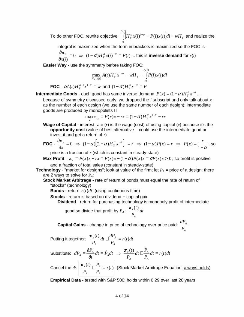
To do other FOC, rewrite objective: [ ] Y

tA

Y wHdiixiPixH −−�−

)(

0

1 )()()( αα and realize the

integral is maximized when the term in brackets is maximized so the FOC is

0)(

�

=∂∂

ixY )()()1( iPixHY =− −ααα ... this is inverse demand for x(i)

Easier Way - use the symmetry before taking FOC:

�−−−)(

0

1

)(,)()()(max

tA

YYixH

diixiPwHxHtAY

αα

FOC - wxHtA Y =−− ααα 11)( and PxHY =− −ααα )1(

Intermediate Goods - each good has same inverse demand ααα −−= xHxP Y)1()( ... because of symmetry discussed early, we dropped the i subscript and only talk about x as the number of each design (we use the same number of each design); intermediate goods are produced by monopolists ∴

rxxHrxxxP Yxx

−−=−= −ααα 1)1()(�max

Wage of Capital - interest rate (r) is the wage (cost) of using capital (x) because it's the opportunity cost (value of best alternative... could use the intermediate good or invest it and get a return of r)

FOC - 0�

=∂

∂x

x [ ] rxHY =−− −αααα )1()1( rxP =− )()1( α α−

=1

)(r

xP , so

price is a fraction of r (which is constant in steady-state) Max Profit - 0)()()1()()(� >=−−=−= xxPxxPxxPrxxxPx αα , so profit is positive

and a fraction of total sales (constant in steady-state) Technology - "market for designs"; look at value of the firm; let PA = price of a design; there

are 2 ways to solve for PA: Stock Market Arbitrage - rate of return of bonds must equal the rate of return of

"stocks" (technology) Bonds - return dttr )( (using continuous time) Stocks - return is based on dividend + capital gain

Dividend - return for purchasing technology is monopoly profit of intermediate

good so divide that profit by PA : dtP

t

A

x )(�

Capital Gains - change in price of technology over price paid: A

A

P

dP

Putting it together: dttrP

dPdt

P

t

A

A

A

x )()(�

=+

Substitute: dtPdtt

PdP A

AA

�=∂

∂= dttrdtP

Pdt

P

t

A

A

A

x )()(�

=+�

Cancel the dt: )()(�

trP

P

P

t

A

A

A

x =+�

(Stock Market Arbitrage Equation; always holds)

Empirical Data - tested with S&P 500; holds within 0.29 over last 20 years

5 of 14

Discounted Profit Stream - based on price of design being equal to present value of all future profits; we'll use non-constant interest rate so instead of e-rt we'll have an integral... this is the way Romer did it

�∞ −�

=t

dssr

A d�eP

�

t τ)(�

)(

Leibnitz Rule (τ not function of t so only 2 terms)

Differentiate wrt t: �∞ −−

�

�

�

� �+

�−==

t

dssr

t

dssr

AA d�e

dt

d�edt

dtP

dt

dP�

t

�

t τ)(�)(�

)()(

�

Look at first term: 1=dt

dt and evaluate at t means t=τ so

)(�)(�

)()(

te�edt

dtt

t

�

t

dssr

t

dssr �−=

�−

−−

Since 0)( =�t

t

dssr , the first term boils down to )(�)(�0 tte −=−

Look at second term: )(� τ isn't a function of t so we can pull it out of the derivative

)()( )(' tftf etfedt

d = ; in this case �−=τ

t

dssrtf )()(

Use Leibnitz Rule again (only 1 term): )()()(' trsrdt

dttf

t==

So right term becomes: ��∞ −∞ − �

=

�

�

�

� �

t

dssr

t

dssr

d�etrd�edt

d�

t

�

t ττ )(�)()(�

)()(

Now pull out the r(t): A

t

dssr

Ptrd�etr

�

t )()(�)()(

=�

�∞ −

τ

Combine terms: AA PtrtP )()(� +−=� )()(�

trP

P

P

t

A

A

A

x =+�

(same equation)

Key Difference - this method gets to stock market arbitrage equation, but can't go the other way because of integration constant; basically we'd have cPA + which explains how we can have "bubbles" in market; stock market arbitrage equation still holds because constant drops out when we differentiate by t, but stock price is actually higher (or lower) than PA

Value of Firm - solve stock market arbitrage equation for PA: AA

xA PPtr

tP

/)(

)(�

�−= ; that's

instantaneous profit divided by instantaneous interest rates minus growth rate of firm Steady-State - both methods gave us the stock market arbitrage; under stead-state:

0=A

A

P

P�

)(

)(

tr

tP x

A

π=

6 of 14

Researcher Wage - productivity per worker times value of output: APtA )(δ

Productivity Per Worker - productivity parameter times number of designs: )(tAδ

Value of Output - we just found that: AP Consumer Behavior - studied producer side for final good, intermediate goods, and

technology; last piece of the puzzle is consumer side; assume utility is discounted at constant rate ρ :

�∞

−−

�

� �

�

−−

0

1

1

1max dte

C tρσ

σ s.t. )()()( tCwtrZtZ −+=�

Constraint - change in assets = interest from assets plus wage minus consumption dynamic optimization... maybe next time

Solution - σ

ρ−= )(tr

C

C�

Slope of consumption (says nothing about level); note, if r↑, slope is steeper (consumers will [eventually] consume more in the future)

Summary of Solution so Far -

(1) αααα αα −−−− == �11

)(

0

11 )()( xHtAdiixHw Y

tA

Y from solving max Y�

(2) ααα −−= xHxP Y)1()( from solving max Y�

(3) α−

=1

)(r

xP from solving max x�

(4) xxPx )(� α= from solving max x�

(5) )(

)(

tr

tP x

A

π= from solving stock market arbitrage eqn

(6) AR PtAw )(δ= researcher wage

(7) σ

ρ−= )(tr

C

C� from consumer behavior

Steady-State Solution - all 7 above hold, but we have steady state number each design

(intermediate goods) so we'll use *x ; also that relates to a single price so **)( PxP = Labor Market Equilibrium - wage in manufacturing of final good (Y) is same as wage of

researchers (so there's no movement of workers form one to the other):

AY PtAxHtAw )(*)()( 11 δα αα == −−

Take (5) and substitute (4): )(

**

tr

xPPA

α=

Substitute (2) into that: [ ]

)(

**)()1(

tr

xxHP Y

A

αααα −−=

t

C C1 (after r↑)

C0

7 of 14

Plug that into the right side of the wage equilibrium equation:

[ ])(

**)()1()(*)()( 11

tr

xxHtAxHtAw Y

Y

αααα ααδα

−−− −==

A bunch of stuff cancels out: )(

)1(1

trHY

αδ −=− )1(

)(

αδ −= tr

HY

4 Equations & 4 Unknowns - solve for HA, HY, g, r

[1] )1(

)(

αδ −= tr

HY from solving labor market equilibrium

[2] AHA

Ag δ==

�

solved when talking about evolution of design

[3] YA HHH += fixed labor

[4] σ

ρ−== )(tr

C

Cg

�

first part is assumption; second part from consumer behavior

Solve [3] for HA and plug it into [2]: )( YHHg −= δ

Substitute HY from [1] into this: α

δαδ

δ−

−=���

����

�

−−=

1

)(

)1(

)( trH

trHg

Solve [4] for r and plug it into this: α

ρσδ−+−=

1

gHg

Solve for g: σα

ρδα

ασ

αρδ

+−−−=

−+

−−

=1

)1(

11

1 HH

g

(Dinopoulos did left version in class; I got second version... they're the same) Policy - what can we do to target g?

Subsidize R&D - δ ↑ g↑ Less Consumption Now - ρ ↓ g↑... not sure you can target patience with policy, but we

can look at societies with higher savings rates (less consumption) and find higher g

Growth Rates - turns out everything grows at g... K

K

Y

Y

C

C

A

Ag

����

====

)(1 tAxHY Yαα −= ... α

YH and α−1x fixed so ln-differentiate trick gives gA

A

Y

Y ==��

xtAK )(= ... x fixed so ln-differentiate trick gives gA

A

K

K ==��

Problem - H in numerator suggests larger H yields larger g; that would suggest U.S. growth is

faster than Hong Kong's (it's not!); also H grows exponentially so g has to grow exponentially (i.e., t → ∞ g → ∞)... that's not realistic either

8 of 14

Schumpeterian Growth - using quality for technological progress

Papers - Segerstrom, et.al. - AER, 1990 Aghion & Howitt - intermediate goods (like Romer); Econometrica, 1992 Grossman & Helpman - continuum of industries; 1991 Dinopoulos - Overview; 1993

Characteristics - Dynamic General Equilibrium Model - can't use partial equilibrium because 1 market

growing could draw resources away from other markets Product Replacement - "creative destruction"; products are replaced by "better" products

(e.g., typewriter, VHS tapes, carburetors) Imperfect Competition - development of new products requires at least temporary

monopoly to do R&D Uncertainty - characterizes all new product development... only about 10% survive

Structure of Model - "all the difficult parts of economics come together" One Good - one industry producing a single consumption good Quality - quality of good can be improved; all "versions" of final good are perfect substitutes R&D Races - uncertainty Two Activities - manufacturing of final output and R&D for quality improvement Full Employment - fixed labor force Monopoly - firm that wins R&D race enjoys monopoly; duration of monopoly depends on

next R&D race Price Limit - price limited by price of previous good and amount of improvement Stock Market - used to finance R&D

Utility - representative consumer has intertemporal utility function: [ ]�∞

− •=0

)(ln dtzeU tρ

Discount rate - ρ

Sub-utility - �� ++++==�∞

=3

32

210

0210 ),,,( xxxxxxxxz

qq

q αααα

Degree of Improvement - α > 1 is degree of quality improvement of product relative to its immediate predecessor

Version of Good - qx ; countably infinite levels of quality

Product Replacement Mechanism - sub-utility above works (in conjunction with pricing) to effectively eliminate previous versions of the final good Example - suppose each worker produces 1 unit of output (x) and use wage of labor as

numeraire; that means 1 worker = 1 unit = $1... MC = AC = 1 Now suppose economy starts with only 0x ; consumers spend all their money on this

good so demand is 0

0 P

Ex = , where E is aggregate expenditures, 0P is price of 0x

Suppose 1x is discovered; consumer utility is 10 xx α+ ; if 0x and 1x are at the same

price, consumer buys all 1x and no 0x ; firm that discovered 1x wants to drive

producer of 0x out of market, but also wants to make as much profit as possible so

he charges the highest price he can for 1x that still has consumers choosing only

1x ... i.e., want to keep utility form 1x higher than utility from 0x : 01 xx ≥α ; if

9 of 14

consumers spend all their money on either good we have 0

0 P

Ex = and

11 P

Ex = ;

substitute these into the utility restriction and solve for 1P :

01 P

E

P

E ≥α 10 PP ≥α

Since minimum price of producer of 0x is MC = wage (w), then the limit price of 1x is

1−≤ qq PP α ; if 1Pw =α , consumers are indifferent between 0x and 1x but assume

hey switch instantaneously (i.e., always choose higher quality when indifferent)

In General - start with utility: q

q

q

q

P

E

P

E αα ≤−

−

1

1 1−≤ qq PP α 1−≤ qq PP α

Profits of Monopolists - assume one worker manufactures one unit of good qx independent of

the level of quality (i.e., doesn’t matter what level of quality is, only takes 1 worker)

qP

E if wPq α≤ (we substitute w (marginal cost) for 1−qP )

0 if wPq α>

Firm Objective - max Ew

EwwxwP qq α

αα

α 1)()(� −=−=−= (i.e., profits are proportional

to consumptions (like the Romer model) Solution - to maximize profit, firm charges maximum price so wPq α=

Model Arrival of Innovations - Poisson Process - characterized by intensity µ ("velocity of innovations")

# of events x that will take place over any interval of length ∆ ~ Poisson

Pr[)( =xg x events occur!

)(]

x

ex ∆∆=µµ

Time T you will have to wait for X to occur ~ Exponential Pr[)( ≡TF event occurs before T Te µ−−= 1] (cdf)

TeTFTf µµ −== )(')( (pdf) ∴ probability that event will occur sometime within the short interval between T and T

+ dt is approximately dte Tµµ −

Instantaneous Probability - dtdte T

Tµµ µ =−

→0lim

instantaneous probability that event doesn't occur is dtµ−1 Expected Time Between Intervals - 1 / µ

Independent Firms - add intensity levels; instantaneous probability is dt)( 21 µµ + ; probability that firms discover innovation at same time is zero

Aggregate Labor - labor used for R&D is L; firm j's labor is Lj so �=j

jLL

Diminishing Returns - measured by 10 ≤< � ... we'll use 1=� to keep things simple

Demand for qx =

tq tq+1

πq

10 of 14

Combine it all: instantaneous probability that at least one firm will discover new product at

time dt is dtLdtdtL �j

j =���

����

�= �µµ )(

"Fair" Research - assume firm j's relative instantaneous probability of success equals its

share of R&D resources: L

L jj =µµ

Probability of Success - individual firm's instantaneous probability of discovering next higher quality good is dtjµ

Solve "fair" research assumption for jµ and sub into this probability: dtL

Ldt j

j µµ =

Sub for µ (i.e., )(Lµ ) from above: dtLLdtL

LLdt j

jj

1)( −== γγµ

Firm Doing R&D - denote discounted earnings of winner of R&D race as )(tV

Expected Discounted Earnings - have to multiply by probability of winning: dtLLtV j1)( −γ

Cost for R&D - dtwL j

Expected Discounted Profits - dtwLdtLLtV jj −−1)( γ

Free Entry - if we assume free entry into R&D Race, expected profits will be zero ∴ 0)( 1 =−− dtwLdtLLtV jj

γ γ−= 1)( wLtV (or if we let 1=� , wtV =)( ); this is the

stock market value of the firm Financing R&D - firms issues stock: "If I win R&D race by time dt, stockholders get monopoly

profit until next R&D race; if I don't win, stockholders get zero"; very risky stock 2 Types of Firms - (1) monopolist producing xq; (2) R&D firms looking for xq+1 Risk Free Return - )(tr ; return on risk free bond in time dt is dttr )( Return for Stock - of firm that has monopoly on current good;

dtLtV

tVdtL

tV

dVdt

tVγγ

)(

0)()1(

)()(

� −−−+

dividends + capital gains * Pr(firm survives) - value of firm * Pr(firm disappears) Note: if L = 0 this is the same as the stock market formula use in Romer Model

Trick - dtVdtt

VdV �=

∂∂=

Portfolio Efficiency - expected return of security of existing monopolist must be equal to the risk free rate of return:

dttrdtLdtLtV

dtVdt

tV)()1(

)()(

�

=−−+ γγ�

dt's cancel: γγ LtrdtLtV

V

tV+=−+ )()1(

)()(

� �

0lim

→dt: γLtr

tV

V

tV+=+ )(

)()(

� �

11 of 14

Solve for V(t):

)()(

�

)(

tV

VLtr

tV�

−+=

γ

Empirical Support - current research shows that this equation works for the S&P 500; doesn't seem to work for individual firms because L is difficult to estimate)

Labor - 1 worker makes 1 unit of output; output is ααE

w

Ex == (since we're assuming w = 1) ∴

number of workers in manufacturing is E/α Confusion over L -

Labor used for R&D is L - this is the original definition Intensity of R&D (Poisson process) is

�

LL =)(µ - we assumed 1=γ so intensity is L

Instantaneous probability that new discovery is made during interval dt is dtLdtL�

=)(µ -

we assumed 1=γ so instantaneous probability is Ldt

For a firm j, this probability is dtLLdt jj1−= γµ

Risk of default is probability of new development in dt which we just said was Ldt if 1=γ

Consumer Maximization - [ ]�∞

− •=0

)(ln max dtzeU t

E

ρ s.t. EwrAtA −+=)(�

(solve in HW)

Solution - ρ−= )(trE

E�

Summary of Model - 6 equations:

(1) Ew

EwwxwP qq α

αα

α 1)()(� −=−=−= (monopoly profits; w = 1)

(2) wPq α= (maximizes monopoly profits; w = 1)

(3) 1)( 1 == −γwLtV (free entry to R&D or zero profit condition; w = 1 and γ = 1)

(4)

)()(

�

)(

tV

VLtr

tV�

−+=

γ (stock market portfolio efficiency condition; γ = 1)

(5) LE

N +=α

(full employment)

(6) ρ−= )(trE

E� (consumer utility maximization)

Steady-State Solution - all 6 equations hold all the time, but in steady state we know that

(6) = 0 so that means ρ=)(tr

From (3) we have 1)( =tV so that means 0)( =tV� ∴ from (4) 1)(

�

)( =+

=Ltr

tV

12 of 14

Sub (1) and ρ=)(tr : 1

1-

)( =+

=L

EtV

ρα

α

Solve for E: )(1

LE +−

= ρα

α... line in (E,L) space (i.e.,

consumption vs. investment) with constant slope (5) gives another line in (E,L) space

Effect of Size of Economy - N ↑ E~

↑ and L~

↑; more population implies more R&D investment so growth increases; this is problem with model so we'll remove the scale effects later

Consumer Patience - ρ ↑ E~

↑ and L~

↓; more impatient (higher discounting for future consumption) means consume more, but invest less

Transitional Dynamics - basically do the same thing we did for steady state,

but we can't assume (6) = 0 From (3) we have 1)( =tV so that means 0)( =tV�

Sub into (4): 1)(

�

)( =+

=Ltr

tV

Solve for profit: Ltr += )(�

That equals (1): ELtrα

α 1)(� −=+=

Solve for interest rate: LEtr −−=α

α 1)(

Sub into (6): ρα

α −−−= LEE

E 1�

Phase Diagram - look at 0=E� ; to determine direction of movement, hold L constant and use E + dE (dE > 0);

0)(1 >−−+−= ρ

αα

LdEEE

E�... that means E increases above 0=E� and decreases

below it There are two stable points on the graph, but neither is a feasible equilibrium

All Consumption - all consumption and no investment is not rational; firm has incentive to do R&D and have monopoly power forever... not realistic

All Investment - the other stable point on the graph doesn't maximize utility because there's no consumption

Steady-State - the steady-state point is an equilibrium, but it is unstable; ∴ transitions are jumps in E and L (realistic because E is chosen by consumers and L by firms and both choices are made instantaneously)

Growth Rate - of utility: [ ]�∞

− •=0

)(ln dtzeU tρ ... really just need to focus on instantaneous utility

[ ] [ ] xqxtz q lnlnln)(ln +== αα

L

E

αN

N

LE

N +=α

(slope is -α)

)(1

LE +−

= ρα

α

(slope is (α - 1)/α)

L~

E~

L

E

αN

N

1N

α

)(1

L+−

ρα

α

α

L~

E~

2N

α

L

E

αN

N

1N

α

)(1 1 L+

−ρ

αα

(slope is (α -

L~

E~

)(1 2 L+

−ρ

αα

(slope is (α -

L

E

αN

N

0=E�

L~

E~

13 of 14

Substitute ααE

w

Ex == : [ ] αα lnlnln)(ln −+= Eqtz

≡),( EtF expected value of instantaneous utility αα lnlnln)( −+= EqE q is number of innovations so (a) it jumps incrementally, (b) is governed by a Poisson

process so LtqE =)( (expected number of innovations from now until time t is Lt

Growth Rate = αlnLt

F =∂∂

∴L (# workers in R&D)↑ growth rate of utility↑

Welfare Analysis - sub ),( EtF into [ ]�∞

− •=0

)(ln dtzeU tρ to compare socially optimal level of

investment and consumption to the levels determined by market equilibrium

[ ]�∞

− −+=0

lnlnln max dtEtLeU t

E,Lααρ s.t. L

EN +=

α

Solve integral first:

[ ] [ ] [ ] [ ]����∞

−∞

−∞

−∞

− −+=−+=0000

lnlnlnlnlnln dtedtEedttLedtEtLeU tttt αααα ρρρρ

Last two integrals are easy because Eln and αln are constant (wrt t):

[ ]ρρ

ρρ Ee

EdtEe tt lnln

ln00

=�

�

−=

∞−

∞−

�

[ ]ρα

ραα ρρ lnln

ln00

=�

�

−=

∞−

∞−

�tt edte

First integral needs integration by parts:

] �� −=b

a

ba

b

a

YdXXYXdY ... let tX = and tedY ρ−= dtX =' and ρρ −= − /teY

[ ] =��

���

��

���

�

�−���

����

�

−−

−∞=

��

���

��

���

−−

�

�

−=

�

� �

�∞−−∞−∞ −∞−∞

−��

02

0

000

0lnlnln

ρρρα

ρραα

ρρρρρρ

tttt eee

Ldtete

LdtteL

222

0

2

ln1lnln

ρα

ρα

ρρα

ρρ LL

eeL =

���

���

=���

���

+−−∞−

Put it all together: ���

����

� +−=+−=ρ

ααρρ

αρα

ρln

lnln1lnlnln

2

LE

LEU

Now it's a static problem: ���

����

� +−=ρ

ααρ

lnlnln

1max

,

LEU

LE s.t. L

EN +=

α

This is a classic consumer optimization problem (standard well, behaved indifference

curves and a linear budget constraint); let solution (social optimum) be )ˆ,ˆ( EL

t

ln(z(t))

ln(z(t))

F(t,E)

Real consumption expenditure

Investment

Discounted

All future growth from investment

14 of 14

Distortion - don't have enough information to give a general statement about the social welfare, but the graphs show that it's possible to have too much investment (too little consumption) or too little investment (too much consumption); usually the latter

L

E

αN

N L~

E~

U1

)(1-

LE += ρα

α

α

L

E U3 U2

Not enough investment (subsidize)

L

E

αN

N L~

E~

U1

)(1-

LE += ρα

α

α

L

E U3 U2

Too much investment (tax)

1 of 2

Scale Effects and Schumpeterian Growth Structure of Growth Models

Labor in Manufacturing - YL

Labor in Research - AL

Output - )()()( tLtAtY Y= (1)

Scale Effect - )(tX is related to scale effects; )(tX ↑ � R&D more difficult

Growth of Technology - )(

)(

)(

)(

tX

tL

tA

tAg A

A ==�

(2)

Labor Market - )()()( tLtLtL AY += (3)

Growth of Labor (Population) - tg NeLtL 0)( = � 0)(

)( ≥=tL

tLg L

�

(constant) (4)

Share of Labor -

Manufacturing Share - )(

)()(

tL

tLtS Y= � Research Share -

)(

)()(1

tL

tLtS A=−

Growth Rate of Per Capital Output - write Y(t) using share of labor: )()()()( tLtStAtY =

Divide by L(t): )()()(

)(tStA

tL

tYy ==

Do ln-differentiate trick: )(ln)(lnln tStAy += � Ay gA

A

y

yg ===

��

(Share of labor in both sectors must be constant in long run) Notation Comment - common to omit (t) argument for variables that are constant in steady

state Scale Effects -

Sub research share into (2): )(

)()1(

tX

tLSg y

−= [1]

Divide (3) by L(t): 1)(

)(

)(

)(

)(

)( =+=tL

tL

tL

tL

tL

tL AY

Sub )()( tXgtL yA = from (2): 1)(

)(=+

tL

gtXS y [2]

Any specification of )(tX must be consistent with these two equations Constant X(t) - Assume 0)( xtX = (constant)

[1] becomes 0

)()1(

x

tLSg y

−= ... which says output grows exponentially (at same rate as

labor force)

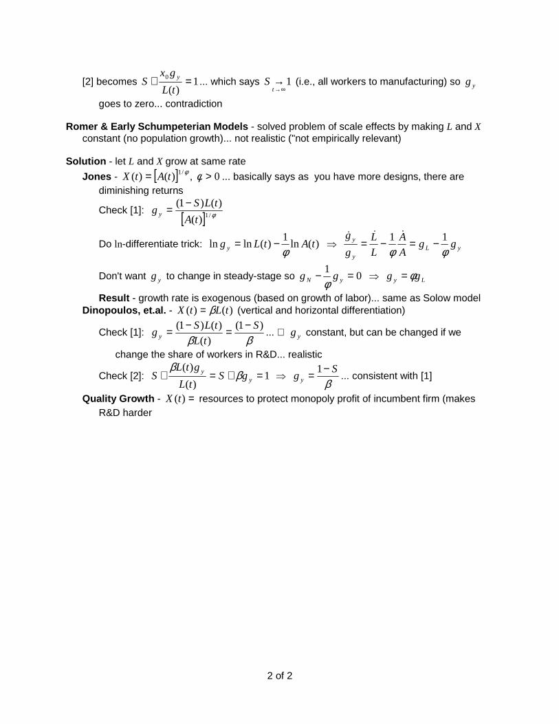
2 of 2

[2] becomes 1)(

0 =+tL

gxS y ... which says 1

∞→→t

S (i.e., all workers to manufacturing) so yg

goes to zero... contradiction Romer & Early Schumpeterian Models - solved problem of scale effects by making L and X

constant (no population growth)... not realistic ("not empirically relevant) Solution - let L and X grow at same rate

Jones - [ ] φ/1)()( tAtX = , 0>φ ... basically says as you have more designs, there are diminishing returns

Check [1]: [ ] φ/1)(

)()1(

tA

tLSg y

−=

Do ln-differentiate trick: )(ln1

)(lnln tAtLg y φ−= � yL

y

y ggA

A

L

L

g

g

φφ11 −=−=

���

Don't want yg to change in steady-stage so 01 =− yN ggφ

� Ly gg φ=

Result - growth rate is exogenous (based on growth of labor)... same as Solow model Dinopoulos, et.al. - )()( tLtX β= (vertical and horizontal differentiation)

Check [1]: ββ

)1(

)(

)()1( S

tL

tLSg y

−=−= ... ∴ yg constant, but can be changed if we

change the share of workers in R&D... realistic

Check [2]: 1)(

)(=+=+ y

y gStL

gtLS β

β �

βS

g y

−= 1... consistent with [1]

Quality Growth - =)(tX resources to protect monopoly profit of incumbent firm (makes R&D harder

1 of 4

ECO 7272, Practice Problem Set 1 Len Cabrera 1. A decrease in the investment rate. Suppose the U.S. Congress enacts legislation that discourages saving and investment, such as the elimination of the investment tax credit that occurred in 1990. As a result, suppose the investment rate falls permanently from s' to s''. Examine the policy change in the Solow model with technological progress, assuming that the economy begins in steady state. Sketch a graph of how (the natural log of) output per worker evolves over time with and without the policy change. Make a similar graph for the growth rate of output per worker. Does the policy change permanently reduce the level or the growth rate of output per worker?

Concept. Don’t think in terms of time; think of the destination (new steady state) and then worry about how you get there. Steady State. Decrease in s causes steady state output per effective worker and capital per effective worker to decline. Based on the formulas:

αkAy~= and Akk /

~= steady state output per worker and capital per worker will also decline. The growth rates, however will not be affected in the steady state:

0~

~

~

~==

k

k

y

y��

and gk

k

y

y ==��

Transition. Focus on two equations that are valid all the time (not just in steady state):

αky~~ = and kgnysk

~)(~~ δ+++=�

The second equation can be rewritten by substituting αky~~ = and dividing both sides

by k~

:

)(~~

~

1δ

α++−=

−gn

k

s

k

k�

This helps us describe the transitional dynamics by plotting 1~ −αks and ).( δ++ gn The difference between the curves gives

kk~

/~� , the growth rate of capital per effective worker; in this

case, the lower savings rate drops the 1~ −αks curve so .0~

/~ <kk�

To determine the effect on output per worker, we start with the modified production function that relates k

~ to y :

αkAy~=

To figure out what happens to y, we do the ln-differentiate trick:

k~

y~

1

~k *

1~y * y~

kgn~

)( δ++

ys ~' ys ~''

* 2

~y

2

~k *

k~

11

~ −αks (n + g + δ)

0~

~<

k

k�

1

~k

2

~k

kk~

/~� starts negative and then gets bigger and bigger as it approaches zero

kk~

/~� at t0 + ∆2

kk~

/~� at t0 + ∆1

12

~ −αks

2 of 4

k

kg

k

k

A

A

y

y~

~

~

~ ���� αα +=+=

We know g doesn't change and we just showed that .0~

/~ <kk� Therefore, output per

worker will grow at a lower rate initially. This rate may be negative if gkk >~/

~�α , but

there is not enough information in the problem to determine if that is the case. We can, however, determine that the growth rate of y will approach the original growth rate in a convex way based on the graph shown earlier. The two cases are shown below (not necessarily to scale). Therefore, the change permanently reduces the level of output per worker.

2. An increase in the labor force. Shocks to an economy, such as wars, famines, or the unification of two economies, often generate large one-time flows of workers across borders. What are the short-run and long-run effects on an economy of a one-time permanent increase in the stock of labor? Examine this question in the context of the Solow model with g = 0 and n > 0.

Steady State. The steady state growth rates are

0==k

k

y

y �� and n

L

L

K

K

Y

Y ===���

therefore, the one time change in the population (L) doesn't affect these rates. Transition. Focus on two equations that are valid all the time (not just in steady state):

αky = and knsyk )( δ++=�

The second equation can be rewritten by substituting αky = and dividing both sides by k :

Time

yy /�

g

Case 2

gkk <~/

~�α

t0 Time

yy /�

g

Case 1

gkk >~/

~�α

t0

Time

yln

t0 Time

yln

t0

Slope of ln y is always g in steady state

y2

k

y y

sy

(n + δ)k

k1

y1

k2

3 of 4

)(1

δα +−= − nk

s

k

k�

This helps us describe the transitional dynamics by plotting 1−αsk and ).( δ+n The difference between the curves gives

kk /� , the growth rate of capital per worker; in this case, the sudden increase in population causes an immediate drop in capital per worker (k). As the transition graph indicates, the lower value of k results in a positive growth rate in k. (Intuitively, what's happening is an increase in capital in order to return to the original level of capital per worker.) To determine the effect on output per worker (y), do the ln-differentiate trick to the intensive form production function:

k

k

y

y �� α=

We just showed that 0/ >kk� , so we also have .0/ >yy� According to the transition graph shown above, these growth rates will drop in a convex way until they return to zero. To relate these growth rates to total capital (K) we look at the definition of k:

kLK = We know L doesn't directly affect K, so this equation explains why k dropped initially. Do the ln-differentiate trick to get:

nk

k

L

L

k

k

K

K +=+=����

Since n is constant, we can ignore that and realize the change in the growth rate of capital is the same as the change in the growth rate of capital per worker. To relate these growth rates to total output (Y) we look at the full production function:

αα −= 1LKY Here we do have an initial effect form the change in L (i.e., Y increases at t0). Do the ln-differentiate trick to get:

nK

K

L

L

K

K

Y

Y)1()1( αααα −+=−+=

����

Again, n is constant so the change in the growth rate of output will mirror the change in the growth rate of capital.

k2 k

1−αsk (n + δ) 0>

k

k�

1k

kk /� starts positive and then gets smaller and smaller as it approaches zero

kk /� at t0 + ∆1 kk /� at t0 + ∆2

Time

yln

t0 Time

kln

t0

Time

yy /�

t0 Time

kk /�

t0

Time

Yln

t0 Time

Kln

t0

Slope of ln Y and ln K is always n in steady state

0

4 of 4

3. An income tax. Suppose the U.S. Congress decides to levy an income tax on both wage income and capital income. Instead of receiving wL + rK = Y, consumers receive (1 - τ)wL + (1 - τ)rK = (1 - τ)Y. Trace the consequences of this tax for output per worker in the short and long runs, starting from steady state.

(1 - τ) cancels so there's no difference in the production function. The per capita capital accumulation function does change:

knsyk )()1( δτ +−−=�

Substitute αky = and divide both sides by k:

)()1(

1 δτα +−−= − n

k

s

k

k�

Steady State.

0)()1(

1 =+−−= − δτα n

k

s

k

k� �

α

δτ −��

���

�

+−=

1

1

)1(*

n

sk

So the income tax effectively lowers the investment rate (same as problem 1).

4. Manna falls faster. Suppose that there is a permanent increase in the rate of technological progress, so that g rises to g'. sketch a graph of the growth rate of output per worker over time. Be sure to pay close attention to the transition dynamics.

Steady State. Increase in g causes stead state capital per worker (k) and output per worker (y) to increase to g'. Transition. Focus on two equations that are valid all the time (not just in steady state):

αky~~ = and kgnysk

~)(~~ δ++−=�

Divide the equation on the left by k~

to see how g relates to the growth rate of k

~:

)(~

~

~1 δα ++−= − gnks

k

k�

Therefore, gkk ∆−=~/

~� (as shown in the first diagram) To figure out what happens to y, we use Ayy /~ = and the ln-differentiate trick we did before:

k

kg

k

k

A

A

y

y~

~

~

~ ���� αα +=+=

We see that when g increases to g', the growth rate of output per worker (y) increases, but the increase is less than ∆g because of the drop in the growth rate of capital per effective worker which equals -∆g (its effect doesn't totally counter ∆g because α < 1). Eventually the growth rate of y will increase to g' as shown in the second diagram.

Time

yy /�

g

t0

g'

k~

1~ −αks

(n + g + δ) 0~

~<

k

k�

(n + g' + δ)

1

~k

2

~k

kk~

/~� starts negative and then gets less and less negative as it approaches zero

kk~

/~� at t0 + ∆2

kk~

/~� at t0 + ∆1

1 of 8

ECO 7272, Practice Problem Set 2 Len Cabrera 1. Consider the following version of a Romer economy. There are only two sectors in the economy: The final goods sector and the research sector. Final output is produced according to the following production function:

�=)(

0

)(lntA

Y diixHY

where YH is the amount of labor in the final goods sector and "ln" denotes the natural logarithm; )(tA is the measure of designs produced by time t, and x is the quantity of design used. The production of designs uses labor and it is governed by the following equation:

A

�H

tA

tA =)(

)(�

Where δ is a productivity parameter, and AH is the amount of labor engaged in research. The full employment condition of labor is given by

YA HHH +=

where H is the fixed supply of labor in the economy. Assume that the government buys every design produced in the research sector by paying a price AP , which should be considered as a fixed parameter in the analysis. In addition, assume that only one unit of each design is needed for final output production, and therefore set 1=x . Perfect competition prevails in all markets and the government expenditure on designs is financed through grants from an international organization. There is no international trade in the model. a. Solve for the balanced growth equilibrium assuming 1=x , and treating AP as a parameter. Calculate the long-run equilibrium values of output growth, and the long-run allocation of labor in production YH and research AH . b. What are the effects of an increase in δ , H , and AP on the balanced growth rate of output and on the growth rate of the wage of labor w ?

a. Growth Rate

1=x � Y

tA

Y HtAdiixHY ln)()(ln)(

0

== �

Do the ln-differentiate trick to get the growth rate of Y: )ln(ln)(lnln YHtAY +=

2 of 8

AY gA

A

Y

Yg ===

��

... growth rate of economy is same as growth rate of A(t)

(HY drops out because it's constant at steady-state; if it wasn't the full employment or labor condition would imply that HA go to zero [or H] because H is fixed.)

Labor Market Workers move between research and manufacturing sectors, so in steady-state

wages in these markets are equal. Assume output Y is numeraire so 1=YP Manufacturing: final good monopoly: XYYYY

HPtAHwHtA

Y

)(ln)(�max −−=

FOC: 0)(�

=−=∂∂

YYY

Y wH

tA

H �

YY H

tAw

)(=

Another Way... marginal product of labor (MPL) YY H

tA

H

Y )(=∂∂

=Yw value of MPL: YY

YY H

tA

H

YPw

)()1(=

∂∂=

Research: same as manufacturing, =Aw value of MPL Value of an innovation is PA

Productivity of all researchers comes from A

�H

tA

tA =)(

)(� � AHt

�AtA )()( =�

Differentiate with respect to HA to get productivity per researcher: )(t�A

∴ AA Pt�Aw )(=

Steady-State Conditions

(1) Growth of output... AAY

�H

tA

tAgg ===

)(

)(�

(2) Labor market wage equilibrium... AY

PtAH

tAw )(

)( δ==

(3) Labor market capacity... YA HHH +=

Solve (2) for HY: AA

Y PPtA

tAH

δδ1

)(

)( ==

Sub HY into this (3) and solve for HA: A

A PHH

δ1−=

Sub HA into (1): AA

Y P

�H

PH

�g

11 −=���

����

�−=

δ

AY P

�Hg

1−=

AY P

Hδ1=

AA P

HHδ1−=

3 of 8

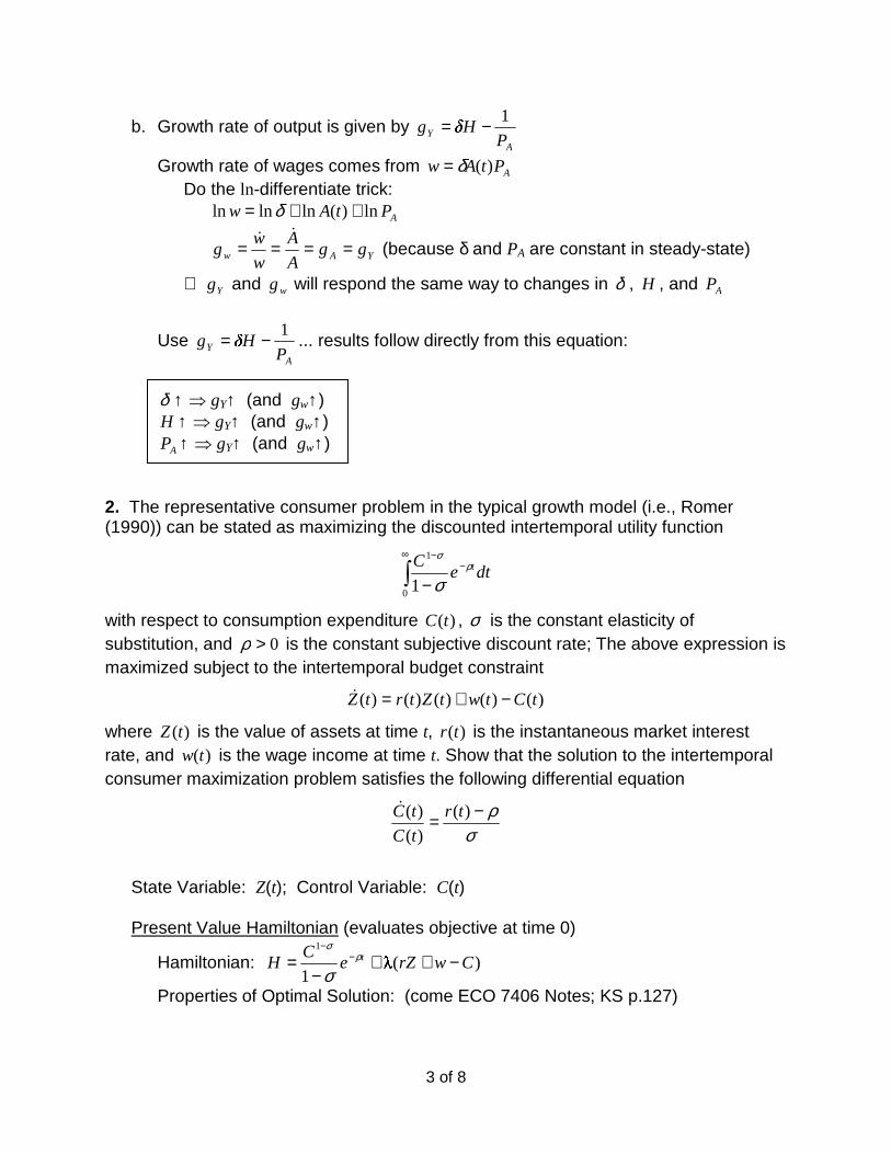
b. Growth rate of output is given by A

Y P

�Hg

1−=

Growth rate of wages comes from APtAw )(δ= Do the ln-differentiate trick:

APtAw ln)(lnlnln ++= δ

YAw ggA

A

w

wg ====

�� (because δ and PA are constant in steady-state)

∴ Yg and wg will respond the same way to changes in δ , H , and AP

Use A

Y P

�Hg

1−= ... results follow directly from this equation:

δ ↑ � gY↑ (and gw↑) H ↑ � gY↑ (and gw↑)

AP ↑ � gY↑ (and gw↑) 2. The representative consumer problem in the typical growth model (i.e., Romer (1990)) can be stated as maximizing the discounted intertemporal utility function

�∞

−−

−0

1

1dte

C tρσ

σ

with respect to consumption expenditure )(tC , σ is the constant elasticity of substitution, and 0>ρ is the constant subjective discount rate; The above expression is maximized subject to the intertemporal budget constraint

)()()()()( tCtwtZtrtZ −+=�

where )(tZ is the value of assets at time t, )(tr is the instantaneous market interest rate, and )(tw is the wage income at time t. Show that the solution to the intertemporal consumer maximization problem satisfies the following differential equation

σρ−= )(

)(

)( tr

tC

tC�

State Variable: Z(t); Control Variable: C(t) Present Value Hamiltonian (evaluates objective at time 0)

Hamiltonian: )(�

1

1

CwrZeC

H t −++−

= −−

ρσ

σ

Properties of Optimal Solution: (come ECO 7406 Notes; KS p.127)

4 of 8

(1) 0�

=−=∂∂ −− teC

C

H ρσ Optimality Condition

(2) �

)('�

rtZ

H −==∂∂− Multiplier Equation

(3) CwrZtZH −+==

∂∂

)('� State Equation

(4) 0)0( ZZ = Boundary Condition (5) ?)(Z =∞ Boundary Condition

(6) 01 ≤−= −−− tCC eCH ρσσ for max Second Order Condition

Solve (2): �)('� rt −= � rtet −=)(�

Solve (1) for C(t): ( )σρσρσρ 111

�rtt

rt

tt

ee

eeC +−

−

−−

=���

����

�=��

�

����

�=

Do the ln-differentiate trick:

( )rtttC +−=��

���

� −−= ρσ

ρσ

1� 1ln1

ln

( )σ

ρρσ

−=+−= rr

C

C 1�

Current Value Hamiltonian (evaluates objective at time t)

Hamiltonian: )(�

1

1

CwrZC

H −++−

=−

σ

σ

(leaves off the te ρ− ; no discounting here)

Properties of Optimal Solution: (given by Prof. Dinopoulos in class)

[1] 0�

=−=∂∂ −σC

C

H

[2] )�

()�

()�

()(�

trtZ

Htt −=

∂∂−= ρρ� (discount rate enters here)

Solve [2] for growth rate: rt

t −= ρ)

�(

)(��

Solve [1] for C: �C1� −

= Do the ln-differentiate trick:

�ln

1ln

σ−=C

σρρ

σσ−=−−=−= r

rC

C)(

1�

�1 ��

5 of 8

3. Consider the following simple version of the Schumpeterian growth model described in Dinopoulos (1996) "Schumpeterian Growth Theory: An Overview." The utility of the representative consumer is given by

�∞

−=0

3 ))(ln()( dttzetU t

where the sub-utility )(tz is defined as ∞

=

=0

210 )5.1(),,,(q

qq xxxxz � . There is only one

industry in the economy, and the arrival of innovations is governed by a Poisson process with intensity L , where L is the amount of R&D researchers employed by firms engaged in sequential R&D races. The economy has 27=N workers that can be allocated between the two activities, manufacturing and R&D. One worker can produce one unit of research services and/or one unit of final consumption good. Use the wage of labor as the numeraire and calculate the stead-state equilibrium values of the following variables: the market interest rate )(tr ; the equilibrium number of R&D workers L ; consumption expenditure E ; the amount of workers in manufacturing; the long-long run growth rate of the economy, g ; the flow of profits at each instant in time

� ; and the stock market valuation of monopoly profits ).(tV

Don't need to do derivation of general equilibrium conditions if we know them; they're included here for easy reference (and studying!)

qP

E if wPq α≤ (we substitute w (marginal cost) for 1−qP )

0 if wPq α>

To max profits firm will charge as much as possible while still driving competitor (maker of 1−qP ) out of the market ∴ wPq α=

Monopoly Profits

αα

w

EwwxwP qq )()(� −=−=

Firm Doing R&D

Pr(firm j making discovery) = dtLLdtL

LLdt j

jj

1)( −== γγµ

Pr(discovery made) = dtLγ )(tV is discounted earnings of winner of R&D race; to get expected discounted

earnings, we have to multiply by probability of winning: dtLLtV j1)( −γ

Cost for R&D = dtwL j

Expected Discounted Profits = dtwLdtLLtV jj −−1)( γ

Demand for qx =

6 of 8

If we assume free entry into R&D Race, expected profits will be zero ∴ dtwLdtLLtV jj −−1)( γ � γ−= 1)( wLtV (stock market value of the firm)

Stock Market Efficiency

Risk free return is )(tr ; return on risk free bond in time dt is dttr )( Return for stock of firm that has monopoly on current good is sum of dividends

plus expected capital games/losses (gains times Pr(firm survives) minus value of firm times Pr(firm disappears)):

dtLtV

tVdtL

tV

dVdt

tVγγ

)(

0)()1(

)()(

� −−−+

Use this trick dtVdtt

VdV �=

∂∂=

Efficiency says: dttrdtLdtLtV

dtVdt

tV)()1(

)()(

�

=−−+ γγ�

dt's cancel: γγ LtrdtLtV

V

tV+=−+ )()1(

)()(

� �

0lim

→dt: γLtr

tV

V

tV+=+ )(

)()(

� �

Solve for V(t):

)()(

�

)(

tV

VLtr

tV�

−+=

γ

Consumer Maximization

[ ]�∞

− •=0

)(ln max dtzeU t

E

ρ s.t. EwrAtA −+=)(�

∞

=

=0

210 ),,,(q

qq xxxxz α� , but qp is set so that none of the previous goods is

purchased so we can use qq xz α=•)( ; also since consumers only purchase

good q, we know αw

E

P

Ex

qq == �

w

E

w

Ez

qq

1

)(−

==• αα

α , so now the

objective is �∞ −

−�

� �

�=

0

1

ln max dtw

EeU

qt

E

αρ

State Variable: A(t); Control Variable: E(t)

Current Value Hamiltonian: )(�

ln1

EwrAw

Eq

−++�

� �

� −α

[1] 0�1 =−=

∂∂

EE

H

7 of 8

[2] )�

()�

()�

()(�

trtA

Htt −=

∂∂−= ρρ�

Solve [2] for growth rate: rt

t −= ρ)

�(

)(��

Solve [1] for E: 1� −=E Do the ln-differentiate trick:

�lnln −=E

ρρ −=−−=−= rrE

E)(�

���

Equilibrium Conditions - General

(1) α

αw

Eww )(� −= (monopoly profits)

(2) γ−= 1)( wLtV (free entry to R&E or zero profit condition)

(3)

)()(

�

)(

tV

VLtr

tV�

−+=

γ (stock market portfolio efficiency condition)

(4) ρ−= )(trE

E� (consumer utility maximization)

(5) LE

N +=α

(full employment condition)

Equilibrium Conditions - For This Problem... 1=γ , 1=w , 5.1=α , 3=ρ , 27=N

[1] EEEw

Eww

3

1

5.1

5.01)(� ==−=−=

αα

αα

[2] 1)( 1 == −γwLtV

[3] �

( )( )

( )( )

V tV t

r t LV t

=+ −

�

[4] 3)( −= trE

E�

[5] LE += 3227

Steady-state � 0=E

E� � from [4] we have 3)( =tr

Since [3] says 1)( =tV , that means 0)( =tV� ∴ from [3] L

tV+

=3

�

)(

Sub [1]: 13

)( 31

=+

=L

EtV � LE 39 +=

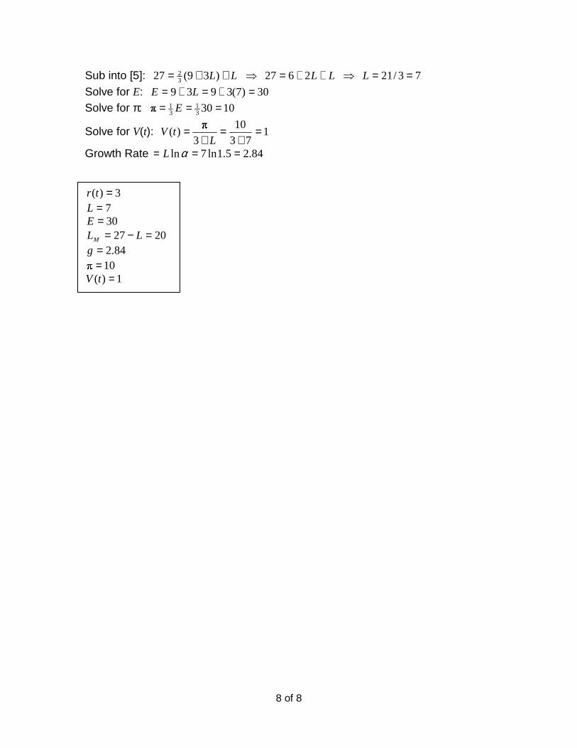
8 of 8

Sub into [5]: LL ++= )39(27 32 � LL ++= 2627 � 73/21 ==L

Solve for E: 30)7(3939 =+=+= LE Solve for π: 1030�

31

31 === E

Solve for V(t): 173

10

3

�

)( =+

=+

=L

tV

Growth Rate 84.25.1ln7ln === αL

3)( =tr 7=L 30=E

2027 =−= LLM 84.2=g

10� = 1)( =tV