Macroeconomics: A Survey of Laboratory Research∗

John DuffyDepartment of EconomicsUniversity of PittsburghPittsburgh, PA 15260 USAEmail: jduffy@pitt.edu

March 2008Comments and Additional Citations Welcome

Abstract

This chapter surveys laboratory experiments addressing macroeconomic phenomena. Thefirst part focuses on experimental tests of the microfoundations of macroeconomic models dis-cussing laboratory studies of intertemporal consumption/savings decisions, time (in)consistencyof preferences and rational expectations. Part two explores coordination problems of interest tomacroeconomists and mechanisms for resolving these problems. Part three looks at experimentsin specific macroeconomic sectors including monetary economics, labor economics, internationaleconomics as well-as large scale, multi-sector models that combine several sectors simultaneously.The final section addresses experimental tests of macroeconomic policy issues.

1 Introduction: Laboratory Macroeconomics

“Economists can do very little experimentation to produce crucial data. This isparticularly true of macroeconomics.” Christopher A. Sims (1996, p. 107)

Macroeconomic theories have traditionally been tested using non-experimental field data, mostoften national income account data on GDP and its components. This practice follows from thewidely-held belief that macroeconomics is a purely observational science: history comes aroundjust once and there are no “do-overs”. Controlled manipulation of the macroeconomy to gaininsight regarding the effects of alternative institutions or policies is viewed as impossible, (not tomention unethical), and so, apart from the occasional natural experiment, many would argue thatmacroeconomic questions cannot be addressed using experimental methods.1

∗Chapter prepared for the Handbook of Experimental Economics Vol. 2, J. Kagel and A.E. Roth, Eds. FrankHeinemann, Rosemarie Nagel, Charles Noussair and Andreas Ortmann provided helpful comments on an earlier draft.

1 Indeed, the term “macroeconomic experiment” does not even typically refer to laboratory experiments involvinghuman subjects but rather to computational experiments using calibrated dynamic stochastic general equilibriummodels as pioneered in the work of Finn Kydland and Edward Prescott (1982). Even these experimental exerciseshave been ruled out as unacceptable by some. Sims again (1996 p. 113) writes: “What Kydland and Prescott callcomputational experiments are computations not experiments. In economics, unlike experimental sciences, we cannotcreate observations designed to resolve our uncertainties about theories; no amount of computation can resolve that.”

1

Yet, as this survey documents, over the past twenty years, a wide variety of macroeconomicmodels and theories have been examined using controlled laboratory experiments with paid hu-man subjects, and this literature continues to grow. The use of laboratory methods to addressmacroeconomic questions has come about in large part due to changes in macroeconomic modeling,though it has also been helped along by changes in the technology for doing laboratory experimen-tation, especially the use of large computer laboratories. The change in macroeconomic modelingis, of course, the now widespread use of explicit micro-founded models of constrained, intertemporalchoice in general equilibrium, game-theoretic or search-theoretic frameworks. The focus of thesemodels is often on how institutional changes or policies affect the choices of decision-makers suchas household and firms, in addition to the more traditional concern with responses in the aggregatetime series data (e.g. GDP) or to the steady states of the model. While macroeconomic modelsare often expressed at an aggregate level, for instance there is a “representative” consumer or firmor a market for the “capital good”, an implicit, working assumption of many macroeconomists isthat aggregate sectoral behavior is not different from that of the individual actors or componentsthat comprise each sector.2 Otherwise, macroeconomists would be obliged to be explicit about themechanisms by which individual choices or sectors aggregate up to the macroeconomic representa-tions they work with, and macroeconomists have been largely silent on this issue. Experimentaliststesting non-strategic macroeconomic models have sometimes taken this representativeness assump-tion at face value, and conducted individual decision-making experiments with a macroeconomicflavor. But, as we shall see, experimentalists have also considered whether small groups of subjectsinteracting with one another via markets or by observing or communicating with one another mightoutperform individuals in tasks that macroeconomic models assign to representative agents.

To date, the main insights gained from macroeconomic experiments include 1) an assessmentof the micro-assumptions underlying macroeconomic models, 2) a better understanding of the dy-namics of expectations which play a critical role in macroeconomic models, 3) a means of resolvingequilibrium selection (coordination) problems in environments with multiple equilibria, 4) valida-tion of macroeconomic model predictions for which field data are not available and 5) the impact ofvarious macroeconomic policy interventions on individual behavior. In addition, laboratory testsof macroeconomic theories have generated new or strengthened existing experimental methodolo-gies including implementation of the representative agent assumption, overlapping generations andsearch-theoretic models, discounting and infinite horizons, methods for assessing equilibration, andthe role of various market clearing mechanisms in characterizing Walrasian competitive equilibrium(for which the precise mechanism of exchange is left unmodeled).

The precise origins of “macroeconomic experiments” is unclear. Some might point to A.W.Phillips’ (1950) experiments using a colored liquid-filled tubular flow model of the macroeconomy,though this did not involve human subjects! Others might cite Vernon Smith’s (1962) doubleauction experiment demonstrating the importance of centralized information to equilibration tocompetitive equilibrium as the first macro-economic experiment. Yet another candidate mightbe John Carlson’s early (1967) experiment examining price expectations in stable and unstableversions of the Cobweb model. However, I will place the origins more recently with Lucas’s 1986

2Of course, this assumption is generally false. As Fisher (1987) points out in his New Palgrave entry on aggregationproblems, “the analytic use of such aggregates as ‘capital’, ‘output’, ‘labour’ or ‘investment’ as though the productionside of the economy can be treated as a single firm is without sound foundation.” Fisher adds that “this has notdiscouraged macroeconomists from continuing to work in such terms.” Indeed, one may think of macroeconomics asan impure language with bad grammar and borrowed words but a language nonetheless, and one with many users.

2

invitation to macroeconomists to conduct laboratory experiments to resolve macro-coordinationproblems that were unresolved by theory. Lucas’s invitation was followed up on by Lim, Prescottand Sunder (1994) and Marimon and Sunder (1993, 1994, 1995), and perhaps as the result of theirinteresting and influential work, over the past decade there has been a great blossoming of researchtesting macroeconomic theories in the laboratory. This literature is now so large that I cannothope to cover every paper in a single chapter, but I do hope to give the reader a good road-map asto the kinds of macroeconomic topics that have been studied experimentally as well as to suggestsome further extensions.

How shall we define a macroeconomic experiment? One obvious dimension to consider is thenumber of subjects. Perhaps Sims’s (and others’) belief that macroeconomic models are difficult totest experimentally hinges on the problem of approximating the large scale of the macroeconomywith the necessarily small numbers of subjects available in laboratory experiments. However, aswe have already noted, in micro-founded models, this issue of the number of subjects employedneed not be the relevant focus. Further, as discussed in this survey, the evidence from manydouble auction experiments beginning with Smith (1962) reveals that equilibration to competitiveequilibrium occurs reliably with just a few (3-5) buyers or sellers on each side of the market, solarge numbers of subjects need not be necessary even in non-strategic market environments.

A second and more sensible approach is simply to define a macroeconomic experiment as onethat tests the predictions of a macroeconomic model or its assumptions, or is framed in the lan-guage of macroeconomics, involving for example, intertemporal consumption and savings decisions,inflation and unemployment, economic growth, bank runs, monetary exchange, monetary or fiscalpolicy or any other macroeconomic phenomena. Unlike microeconomic models and games whichoften strive for generality, macroeconomic models are typically built with a specific macroeconomicstory in mind that is not as easily generalized to other non-macroeconomic settings. For thisreason, our definition of a macroeconomic experiment may be too restrictive. There are manymicroeconomic experiments - coordination games for instance - that can be given a macroeco-nomic interpretation. In discussing those studies as macroeconomic experiments, I will attempt toemphasize the macroeconomic interpretation.

The coverage of this chapter can be viewed as an update on topics covered in several chapters ofthe first volume of the Handbook of Experimental Economics, including discussions of intertemporaldecision-making by Camerer (1995), coordination problems by Ochs (1995) and asset prices bySunder (1995), though the coverage here will not be restricted to these topics alone. Most ofthe literature surveyed here was published since 1995, the date of the first Handbook volume. Inaddition, this chapter builds on, complements and extends earlier surveys of the macroeconomicexperimental literature by myself, Duffy (1998, 2008), and by Ricciuti (2004).

2 Dynamic, Intertemporal Optimization

Perhaps the most widely-used model in modern macroeconomic theory is the one-sector, infinitehorizon optimal growth model pioneered by Ramsey (1928) and further developed by Cass (1965)and Koopmans (1965). This model posits that individuals solve a dynamic, intertemporal opti-mization problem in deriving their consumption and savings plan over an infinite horizon. Bothdeterministic and stochastic versions of this model are workhorses of modern real business cycletheory and growth theory.

In the urge to provide microfoundations for macroeconomic behavior, modern macroeconomists

3

assert that the behavior of consumers or firms can be reduced to that of a representative, fullyrational individual actor; there is no room for any “fallacies of composition” in this framework.It is therefore of interest to assess the extent to which macroeconomic phenomena can be said toreflect the choices of individuals facing dynamic stochastic intertemporal optimization problems.Macroeconomists have generally ignored the plausibility of this choice-theoretic assumption pre-ferring instead to examine the degree to which the time series data on GDP and its componentsmove in accordance with the conditions that have been optimally derived from the fully rationalrepresentative agent model and especially whether these data react predictably to shocks or policyinterventions.

2.1 Optimal Consumption/Savings Decisions

Whether individuals can in fact solve a dynamic stochastic intertemporal optimization problem ofthe type used in the one-sector optimal growth framework has been the subject of a number oflaboratory studies, including Hey and Dardanoni (1988), Carbone and Hey (2004), Noussair andMatheny (2000), Lei and Noussair (2002), and Ballinger et al. (2003). These studies take therepresentative agent assumption of modern macroeconomics seriously and ask whether subjectscan solve a discrete-time optimization problem of the form:

max{ct}

Et

∞Xt=0

βtu(ct)

subject to:ct + xt ≤ ωt,

where ct is time t consumption, u(·) is a concave utility function, β is the period discount factor,xt represents time t savings (if positive) or borrowings (if negative) and ωt is the household’s timet wealth.

Hey and Dardanoni (1988) assume an endowment economy, where wealth evolves accordingto ωt = R(ωt−1 − ct−1) + yt, with ω0 > 0 given. Here, R denotes the (constant) gross return onsavings and yt is the stochastic time t endowment of the single good; the mean and variance of thestochastic income process is made known to subjects. By contrast, Noussair and associates assume anon-stochastic production economy, where ωt = f(kt)+(1−δ)kt, with f(·) representing the known,concave production function, kt denoting capital per capita and δ denoting the depreciation rate.In this framework, it is public knowledge that all of an individual’s savings st, are invested in capitaland become the next period’s capital stock, i.e., xt = kt+1. The dynamic law of motion for theproduction economy is expressed in terms of capital rather than wealth: kt+1 = f(kt)+(1−δ)kt−ct,with k0 > 0 given. The gross return on savings is endogenously determined by R = f 0(kt)+(1− δ).

Solving the maximization problem given above, the first order conditions imply that the optimalconsumption program must satisfy the Euler equation:

u0(ct) = βREtu0(ct+1),

where the expectation operator is with respect to the (known) stochastic process for income (orwealth). Notice that the Euler equation predicts a monotonic increasing, decreasing or constantconsumption sequence, depending on whether βR is less than, greater than or equal to 1. Solving fora consumption or savings function involves application of dynamic programming techniques that

4

break the optimization problem up into a sequence of two-period problems; the Euler equationabove characterizes the dynamics of marginal utility in any two periods. For most specificationsof preferences, analytic closed-form solutions for the optimal consumption or savings function arenot possible, though via concavity assumptions, the optimal consumption/savings program can beshown to be unique.

In testing this framework, Hey and Dardanoni (1988) addressed several implementation issues.First, they had to rule out borrowing (negative saving) so as to prevent subjects from endingthe session in debt. Second, they attempted to implement discounting and the stationarity as-sociated with an infinite horizon by having a constant probability that the experimental sessionwould continue with another period. Finally, rather than inducing a utility function, they supposedthat all subjects had constant absolute risk aversion preferences and they estimated each individ-ual subject’s coefficient of absolute risk aversion using data they gathered from hypothetical andpaid choice questions presented to the subjects. Given this estimated utility function, they thennumerically computed optimal consumption for each subject and compared it with their actualconsumption choice. To challenge the theory, they consider different values for R and β as well asfor the parameters governing the stochastic income process, y.

They report mixed results. First, consumption is significantly different from optimal behavior;in particular, there appears to be great time-dependence in consumption behavior, i.e., consump-tion appears dependent on past income realizations, which is at odds with the time-independentnature of the optimal consumption program. Second, they find support for the comparative staticimplications of the theory. That is, changes in the discount factor β or in the return on savings, Rhave the same effect on consumption as under optimal consumption behavior. So they find mixedsupport for dynamic intertemporal optimization.

Carbone and Hey (2004) attempt to simplify the design of Hey and Dardanoni in several re-spects. First, they eliminate discounting and consider a finite horizon, 25 period model. Theyargue, based on the work of Hey and Dardanoni, that subjects “misunderstand the stationarityproperty” of having a constant probabilistic stopping rule. Second, they greatly simplify the sto-chastic income process, allowing there to be just two values for income — one “high” which they referto as a state where the consumer is “employed” and the other “low” in which state the consumeris “unemployed.” They use a two-state Markov process to model the state transition process: con-ditional on being employed (unemployed), the probability of remaining (becoming) employed wasp(q), and these probabilities were made known to subjects. Third, rather than infer preferencesthey induce a constant absolute risk aversion utility function. Their treatment variables were p, q,R and the ratio of employed to unemployed income; they considered two values of each, one highand one low, and examined how consumption changed in response to changes in these treatmentvariables relative to the changes predicted by the optimal consumption function (again numericallycomputed). Table 1, shows a few of their comparative static findings.

An increase in the probability of remaining employed caused subjects to overreact in theirchoice of additional consumption relative to the optimal change regardless of their employmentstatus (Unemployed or employed), whereas an increase in the probability of becoming employed —a decrease in the probability of remaining unemployed — led to an under-reaction in the amountof additional consumption chosen relative to the optimal prediction. On the other hand, theeffect of a change in the ratio of high-to-low income on change in consumption was quite close tothe optimum change. Carbone and Hey emphasize also that there was tremendous heterogeneityin terms of subjects’ abilities to confront the life-cycle consumption savings problem, with most

5

Change (∆) in treatment variable Unemployed Employed(from low value to high value) Optimal Actual Optimal Actual∆p (Pr. remaining employed) 5.03 23.64 14.57 39.89∆q (Pr. becoming employed) 14.73 -1.08 5.68 0.15∆ ratio high-low income 0.25 0.24 0.43 0.76

Table 1: Average Change in Consumption in Response to Parameter Changes and Conditional onEmployment Status, taken from Carbone and Hey (2004,Table 5).

applying too short, or too variable a planning horizon to conform to optimal behavior. Theyconclude that “subjects do not seem to be able to smooth their consumption stream sufficiently —with current consumption too closely tracking current income.” Interestingly, the excess sensitivityof consumption to current income (in excess of that warranted by a revision in expectations of futureincome) is a well-documented empirical phenomenon in studies of consumption behavior using fielddata (see, e.g., Flavin (1981), Hayashi (1982), or Zeldes (1989)). This corroboration of evidencefrom the field should give us further confidence in the empirical relevance of the laboratory analysesof intertemporal consumption-savings decisions. Two explanations for the excess sensitivity ofconsumption to income that have appeared in the literature are 1) binding liquidity constraintsand 2) the presence of a precautionary savings motive, (which is more likely in a finite horizonmodel). Future experimental research might explore the relative impacts of these two factors onconsumption decisions.

Noussair and Matheny (2000) depart from the work of Hey and associates by adding a concaveproduction technology, f(kt) = Akαt , α < 1, which serves to endogenize the return on savings in con-formity with modern growth theory. They induce both the production function and a logarithmicutility function by giving subjects schedules of payoff values for various levels of k and c, and theyimplement an infinite horizon by having a constant probability that a sequence of rounds continues.Subjects made savings decisions (chose xt = kt+1) with the residual from their budget constraintrepresenting their consumption. Noussair and Matheny varied two model parameters, the initialcapital stock, k0 and the production function parameter α. Variation in the first parameter changesthe direction by which paths for consumption and capital converge to steady state values (fromabove or below) while variations in the second parameter affect the predicted speed of convergence;the lower is α, the greater is the speed of convergence of the capital stock and consumption to thesteady state of the model. Among the main findings, Noussair and Matheny report that sequencesfor the capital stock are monotonically decreasing regardless of parameter conditions and theoreti-cal predictions with regard to speed of convergence do not find much support. Consumption is, ofcourse linked to investment decisions and is highly variable. They report that subjects occasionallyresorted to consumption binges, allocating nearly nothing to the next period’s capital stock, incontrast to the prediction of consumption smoothing, however, this behavior seemed to lessen withexperience. A virtue of the Noussair-Matheny study is that it was conducted with both U.S. andJapanese subjects, with similar findings for both countries.

One explanation for the observed departure of behavior from the dynamically optimal path isthat the representative agent assumption, while consistent with the reductionist view of modern

6

macroeconomics, assumes too much individual rationality to be useful in practice.3 Informationon market variables (e.g., prices) as determined by many different interacting agents, may be anecessary aid to solving such complicated optimization decisions. An alternative explanation maybe that the standard model of intertemporal consumption smoothing abstracts away from theimportance of social norms of behavior with regard to consumption decisions. Akerlof (2007), forinstance, suggests that people’s consumption decisions may simply reflect their “station in life”.College students (the subjects in most of these experiments) looking to their peers, choose to live likecollege students with expenditures closely tracking income. Both of these alternative explanationshave been considered to some extent in further laboratory studies.

Ballinger et al. (2003) explore the role of social learning in a modified version of the noisy en-dowment economy studied by Hey and Dardanoni (1988). In particular, they eliminate discounting(presumably to get rid of time dependence) focusing on a finite 60-period horizon. Subjects arematched into three-person ”families” and make decisions in a fixed sequence. The generation 1(G1) subject makes consumption decisions alone for 20 periods; in the next 20 periods (21-40) hisbehavior is observed by the generation 2 (G2) subject, and in one treatment, the two are free tocommunicate with one another. In the next twenty periods (periods 41-60 for G1), (periods 1-20for G2), both make consumption/savings decisions. The G1 subject then exits the experiment.The same procedure is then repeated with the generation 3 (G3) subject watching the G2 subjectfor the next twenty rounds etc. Unlike Hey and Dardanoni, Ballinger et al. induce a constant rela-tive risk aversion utility function on subjects using a Roth-Malouf (1979) binary lottery procedure.This allows them to compute the path of optimal consumption/savings behavior. These preferencesgive rise to a precautionary savings motive wherein liquid wealth (saving) follows a hump-shapedpattern over the 60-period lifecycle.

Ballinger et al.’s (2003) main treatment variable concerns the variance of the stochastic incomeprocess (high or low) which affects the peak of the precautionary savings hump; in the high case theyalso explore the role of allowing communication/mentoring or not (while maintaining observabilityof actions by overlapping cohorts at all times). Among their findings, they report that subjects tendto consume more than the optimal level in the early periods of their lives leading to less savings andbelow optimal consumption in the later periods of life. However, savings is greater in the high ascompared with the low variance case which is consistent with the comparative static prediction ofthe rational intertemporal choice framework. They also find evidence for time-dependence in thatconsumption behavior is excessively sensitive to near lagged changes in income. Most interestingly,they report that consumption behavior of cohort 3 is significantly closer to the optimal consumptionprogram than in the consumption behavior of cohort 1 suggesting that social learning by observationplays an important role, and may be a more reasonable characterization of the representative agent.

Lei and Noussair (2002) pursue a complementary approach in the optimal growth model withcapital. They contrast the “social planner” case, where a single subject is charged with maximizingthe representative consumer-firms’ present discounted sum of utility from consumption over anindefinite horizon (as in Noussair and Matheny (2000)), with a decentralized market approachwherein the same problem is solved by five subjects looking at price information. In this markettreatment the production and utility functions faced by the social planner are disaggregated intofive individual functions assigned to the five subjects; that aggregate up to the same functionsfaced by the social planner. For example, some subjects had production functions with marginal

3See Kirman (1992) for a discussion of the limitations of the representative agent assumption.

7

products for capital that were higher than for the economy-wide production function while othershad marginal products for capital that are lower. At the beginning of a period, production tookplace, based on previous period’s capital, using either the individual production functions in themarket treatment or the economy-wide production function in the social planner treatment. Next,in the market treatment, a double auction market for output (or potential future capital) openedup. Agents with low marginal products of capital could trade some of their output to agents withhigh marginal products for capital in exchange for experimental currency units (subjects were givenan endowment of such units each period, which they had to repay). The import of this design wasthat the market effectively communicated to the five subjects the market price of a unit of output(or future capital). As future capital could be substituted one-for-one with future consumption, themarket price of capital revealed to subjects the marginal utility of consumption. After the marketfor output closed, subjects in the market treatment could individually allocate their adjusted outputlevels between future capital kt+1 or savings, and experimental currency units or consumption ct.By contrast, in the social planner treatment, there was no market for output; the representativeindividual proceeded directly to the step of deciding how to allocate output between future capital(savings) and current consumption. At the end of the period, subjects’ consumption amounts wereconverted into payoffs using the economy-wide or individual concave utility functions and loans ofexperimental currency units in the market treatment were repaid.

[Insert Figure 1 here.]

The difference in consumption behavior between the market and representative agent-socialplanner treatments is illustrated in Figure 1, which shows results from a representative session ofone of Lei and Noussair’s treatments. In the market treatment, there was a strong tendency forconsumption (as well as capital and the price of output) to converge to their unique steady statevalues, while in the social planner treatment, consumption was typically below the steady statelevel and much more volatile.

In further analysis, Lei and Noussair (2002) make use of a linear, panel data regression modelto assess the extent to which consumption and savings (or any other time series variable for thatmatter) can be said to be converging over time toward predicted (optimal) levels.4 In this regressionmodel, yj,t denotes the average (or economy-wide level) of the variable of interest by cohort/sessionj in period t = 1, 2, ... and Dj is a dummy variable for each of the j = 1, 2..., J cohorts. Theregression model is written as:

yj,t = α1D1

t+ α2

D2

t...+ αJ

DJ

t+ β

t− 1t

+ j,t, (1)

where j,t is a mean zero, random error term. The αj coefficients capture the initial starting valuesfor each cohort while the β coefficient captures the asymptotic value of the variable y to which allJ cohorts of subjects are converging; notice that the α coefficients have a full weight of 1 in theinitial period 1 and then have exponentially declining weights while the single β coefficient has aninitial weight of zero that increases asymptotically to 1. For the dependent variable in (1), Lei andNoussair (2002) use: 1) the consumption and capital stocks (savings) of cohort j, cj,t, and kj,t+1,2) the absolute deviation of consumption from its optimal steady state value, |cj,t− c∗|, and 3) the

4This regression model was first proposed to study the convergence of experimental panel data in Noussair et al.(1995).

8

ratio of the realized utility of consumption to the optimum, u(cj,t)/u(c∗). For the first type ofdependent variable, the estimate β̂ reveals the values to which the dependent variable, cj,t and kj,tare converging across cohorts; strong convergence is said to obtain if β̂ is not significantly differentfrom the optimal steady state levels, c∗ and k∗. For the second and third types of dependentvariable, one looks for whether β̂ is significantly different from zero or one, respectively. Lei andNoussair (2002) also consider a weaker form of convergence that examines whether β̂ is closer (inabsolute value) to the optimal, predicted level than a majority of the α̂j estimates. Using allfour dependent variables, they report evidence of both weak and strong convergence in the markettreatment, but only evidence of weak (and not strong) convergence in the social planner treatment.5

Tests of convergence based on the regression model (1) are found in several experimental macro-economic papers reviewed later in this chapter, and so I take the opportunity here to briefly com-ment on this model. First, the notion that strong convergence obtains if β̂ is not significantlydifferent from the predicted level, y∗, while weak convergence obtains if |β̂ − y∗| < |α̂j − y∗| for amajority of j’s is somewhat problematic, as strong convergence need not imply weak convergence,as when the α̂j estimates are insignificantly different from β̂. Second, if convergence is truly thefocus, an alternative approach would be to use an explicitly dynamic adjustment model for eachcohort j of the form:

yj,t = λjyj,t−1 + μj + j,t. (2)

Using (2), weak convergence would obtain if the estimates, λ̂j , were significantly less than 1,

while strong convergence would obtain if the estimate of the long-run expected value for yj ,μ̂j

1−λ̂j,

was not significantly different from the steady state prediction y∗; in this model, strong convergenceimplies weak convergence, and not the reverse.6 Finally, analysis of joint convergence across the Jcohorts to the predicted level y∗ could be studied through tests of the hypothesis:

IJ

⎛⎜⎝ μ̂1...μ̂J

⎞⎟⎠+⎛⎜⎝ λ̂1

...λ̂J

⎞⎟⎠ y∗ =

⎛⎜⎝ y∗

...y∗

⎞⎟⎠ ,

where IJ is a J-dimensional identity matrix.

2.2 Exponential discounting and infinite horizons

It is common in macroeconomic models to assume infinite horizons, as the representative householdis typically viewed as a dynasty, with an operational bequest motive linking one generation with thenext. Of course, infinite horizons are not operational but indefinite horizons are. As we have seen,in experimental studies, these have often been implemented by having a constant probability δ thata sequence of decision rounds continues with another round.7 Theoretically this practice should

5Lei and Noussair (2002) also consider a planning agency treatment in which the social planner is replaced witha group of five subjects (as in the market treatment) who together attempt to solve the social planner’s problem.Convergence results for this planning agency treatment are somewhat better than in the social planner treatmentbut still worse than in the market treatment, based on regression findings using the model (1)

6Starting in period 1 with yj,1 and iterating on (2) we can write E[yj,t] = λt−1j yj,1 +t−2i=0 λ

iμj +t−2i=0 λ

ij j,t−i.

Given λ < 1, and for t sufficiently large, we have E[yj ] =μj

1−λj.

7The issue of whether the length of time taken up by a decision round matters is an unexplored issue. This issueis tied up with aggregation of decisions. Macroeconomic data are typically recorded at low frequencies, e.g., monthly

9

induce both exponential discounting of future payoffs at rate δ per round as well as the stationarityassociated with an infinite horizon, in the sense that, for any round reached, the expected numberof future rounds to be played is always δ + δ2 + δ3 + ..., or 1

1−δ .

To better induce discounting at rate δ it is desirable to have subjects participate in severalindefinitely repeated sequences of rounds within a given session - as opposed to a single indefinitelyrepeated sequence — as the former practice provides subjects with the experience that a sequenceends and thus a better sense of the intertemporal rate of discount they should apply to payoffs. Afurther good practice is to make transparent the randomization device for determining whether anindefinite sequence continues or not, e.g., by letting the subjects themselves roll a die at the endof each round using a rolling cup. A difficult issue is the possibility that an indefinite sequencecontinues beyond the scheduled time of a session. This may often be avoided by choosing a discountfactor that is not too high. Of course, a discount factor should also not be so low that one-round(single-shot) sequences are a frequent occurrence. A good compromise might be to set δ to .80,implying an expected duration of 5 rounds from the start of each sequence (as well as from anyround reached!).8 Another good practice is to recruit subjects for a longer period of time thannecessary, say several hours, and inform them that a number of indefinitely repeated sequencesof rounds will be played for a set amount of time — say for one hour following the reading ofinstructions. Subjects would be further instructed at the outset of the session, that after thatset amount of time had passed, the indefinite sequence of rounds currently in play would be thelast indefinite sequence of the experimental session. In the unlikely event that this last indefinitesequence continued beyond the long period scheduled for the session, subjects would be instructedthat they would have to return at a set date to complete that indefinite sequence.

In practice, as we have seen, some researchers feel more comfortable working with finite horizonmodels. However, replacing an infinite horizon with a finite horizon may not be innocuous; thischange may greatly alter predicted behavior relative to the infinite horizon case. For instance,the finite horizon life-cycle model of the consumption savings decision greatly increases the extentof the precautionary savings motive relative to the infinite horizon case. Other researchers havechosen not to tell subjects when a sequence of decision rounds is to end as a way of implementingan indefinite horizon. A difficulty with that practice is that the experimenter loses control ofsubjects’ expectations regarding the likely continuation of a sequence of decisions and appropriatediscounting of payoffs. This can be a problem if, for instance, the existence of equilibria dependon the discount factor being sufficiently high. Yet another approach is to terminate a session aftera finite number of rounds, but exponentially discount the payoffs subjects receive in each roundleading up to the terminal round. The problem with this approach of course, is that does notimplement the stationarity associated with an infinite horizon.

or quarterly “consumption,” whereas in laboratory studies, the length of time between decisions is, out of necessity,much more compressed — a few seconds to a few minutes.

8This can be implemented using any fair randomization device, e.g., cards, balls in a bingo cage or dice. If usingdice, it is best to use the five convex regular polyhedra (the platonic solids), i.e., 4-, 6-, 8-, 12-, or 20-sided dice which,when manufactured precisely, are regarded as “fair”. Perhaps the simplest procedure is to roll a six-sided die at theend of each round and state that the game continues with another round so long as a six is not rolled, thus inducingδ = .833.

10

2.3 Exponential or Hyperbolic Discounting?

Recently, there has been a revival of interest in time-inconsistent preferences with regard toconsumption-savings decisions, where exponential discounting is replaced by a quasi-hyperbolicform so that the representative agent is viewed as maximizing

u(ct) + βTXi=1

δiu(ct+i),

where δ ∈ (0, 1) is a discount factor and the parameter β ≤ 1 characterizes the agent’s bias—for—the—present (exponential discounting has β = 1). Agents who discount hyperbolically (β < 1)rather than exponentially may exhibit time-inconsistent behavior (self-control problems) in thatthey systematically prefer to reverse earlier decisions, e.g., regarding how much they have saved.Thus, a possible explanation for the departures from optimal consumption paths noted above inexperimental studies of intertemporal decision-making may be that subjects have such present-biased preferences. Indeed, Laibson (1997), O’Donoghue and Rabin (1999) and several others haveshown that consumers with such preferences save less than exponential consumers.

Although time-inconsistent preferences have been documented in numerous psychological stud-ies (see, e.g. Frederick et al. (2002) for a survey) the methodology used has often consisted ofshowing inconsistencies in hypothetical (i.e. unpaid) money-time choices (e.g., Thaler (1981)). Forexample, subjects are asked whether they would prefer $D now or $D(1 + r) t periods from now,where variations in both r and t are used to infer individual rates of time preference. Recently, non-hypothetical (i.e. paid) money-time choice experiments have been conducted that more carefullyrespect the time dimension of the trade-off (e.g. Coller et al. (2005) and Benhabib et al. (2006)).These studies cast doubt on the notion that discounting is consistent with either exponential orquasi-hyperbolic models of discounting. For instance, Benhabib et al. (2006) report that discountrates appear to vary with both the time delay from the present and the amount of future rewardsin contrast to exponential discounting. However, Coller et al. (2005) show that in choices betweenmoney rewards to be received only in the future, e.g., 7 days from now versus 30 days from now,variations in the time delay between such future rewards do not appear to affect discount rates,which is consistent with both exponential and quasi-hyperbolic discounting, but inconsistent withcontinuous hyperbolic discounting. Consistent with quasi-hyperbolic discounting, both studies findthat a small fixed premium attached to immediate versus delayed rewards, can reconcile much ofthe variation in discount rates between the present and the future and between different futurerewards. However, this small fixed premium does not appear to vary with the amount of futurerewards (Benhabib et al.) and may simply reflect transaction/credibility costs associated with re-ceiving delayed rewards (Coller et al.) making it difficult to conclude definitively in favor of thequasi-hyperbolic model.

Even more recently, Anderson et al. (2007) make a strong case that time preferences cannot beelicited apart from risk preferences. Prior studies on time discounting all presume that subjects haverisk neutral preferences. However, if subjects have risk averse preferences (concave utility functions)as is typically the case, the implied discount rates from the binary time preference choices will belower than under the presumption of risk neutrality (linear utility functions). Indeed, Andersonet al. (2007) elicit joint time and risk preferences by having each subject complete sequences ofbinary lottery choices (of the Holt-Laury (2002) variety) that are designed to elicit risk preferencesas well as sequences of binary time preference choices that are designed to elicit their discount rates

11

(similar to those in the Coller et al. study). They find that once the risk aversion of individualsubjects is taken into account, the implied discount rates are much lower than under the assumptionof risk neutral preferences. This finding holds regardless of whether discounting is specified to beexponential or quasi-hyperbolic or some mixture.

While it is standard practice to implement exponential discounting in laboratory studies asmost theories with indefinite horizons presume time-consistent preferences, it might be of interest toattempt to induce hyperbolic discounting (perhaps with an effort made to control for risk aversion,e.g., via the use of a Roth-Malouf (1979) binary lottery) by letting the probability of continuation(the discount factor) be time-dependent, i.e., δt = 1

1+rt , where r is the rate of time preferenceused in exponential discounting and t indexes time t = 1, 2, .... One might then assess whether thisdifferent stochastic process for ending an indefinite sequence affected consumption-savings behaviorrelative to the case of exponential discounting.

2.4 Expectation Formation

In modern, self-referential macroeconomic models, expectations of future endogenous variables playa critical role in the determination of the current values of those endogenous variables, i.e. beliefsaffect outcomes which in turn affect beliefs which affect outcomes, etc. Since Lucas (1972) it hasbecome standard practice to assume that agents’ expectations are rational in the sense of Muth(1961) and indeed most models are “closed” under the rational expectations assumption. The use ofrational expectations to close self-referential models means that econometric tests of these modelsusing field data are joint tests of the model and the rational expectations assumption, confoundingthe issue of whether the expectational assumption or other aspects of the model are at fault ifthe econometric evidence is at odds with theoretical predictions. While many tests of rationalexpectations have been conducted using survey data, (e.g. Frankel and Froot (1987)), these testsare beset by problems of interpretation, for example due to uncontrolled variations in underlyingfundamental factors, or to the limited incentives of forecasters to provide accurate forecasts, etc.In the lab it is possible to exert more control over such confounding factors as well as to implementthe self-referential aspect of macroeconomic models.

Early experimental tests of rational expectations involved analyses of subjects’ forecasts of ex-ogenously given stochastic processes for prices, severing the critical self-referential aspect of macro-economic models, but controlling for potentially confounding changes in fundamental factors (seee.g., Schmalensee (1976) or Dwyer et al. (1993)). Later experimental tests involved elicitation ofprice forecasts from subjects who were simultaneously participants in experimental asset marketsthat were determining the prices being forecast (Williams (1987), Smith et al. (1988)). Marimonand Sunder (1993, 1994) were the first to elicit inflation forecasts which were then used to deter-mine subjects’ intertemporal consumption/savings decision and via market clearing the actual pricelevel. Subjects were not aware of the overlapping generations model in which they were operating- instead they were engaged in a forecasting game, with optimal savings decisions being made forthem by a computer program. As discussed in the prior handbook surveys by Camerer (1995) andOchs (1995), many (though not all) of these papers found little support for rational expectationsin that forecast errors tended to have non-zero means and were autocorrelated or were correlatedwith other observables. Further, the path of prices sometimes departed significantly from rationalexpectations equilibrium. However, most of these experimental studies involve analyses of priceforecasts in environments where there is no explicit mechanism by which forecasts determine sub-

12

sequent outcomes as is assumed in forward—looking macroeconomic models (Marimon and Sunder(1993, 1994) being an exception). Further, some of these experimental tests, e.g. Smith et al.(1988) involved analyses of price forecasts for relatively short periods of time or in empirically non-stationary environments where trading behavior resulted in price bubbles and crashes, providing aparticularly challenging test for rational expectations hypothesis.

More recently some macroeconomists have come to believe that rational expectations presumestoo much knowledge on the part of the agents who reside within these models. For instance,rational expectations presumes common knowledge of rationality. Further, rational expectationsagents know with certainty the underlying model whereas econometricians are often uncertain ofdata generating processes and resort to specification tests. Given these strong assumptions, someresearchers have chosen to replace rational expectations with some notion of bounded rationalityand ask whether boundedly rational agents operating for some length of time in a known, stationaryenvironment might eventually learn to possess rational expectations from observation of the relevanttime series data (see e.g., Sargent (1993, 1999) and Evans and Honkapohja (2001) for surveys ofthe theoretical literature).

Two notions of boundedly rational expectation formation are found in the experimental liter-ature relevant to macroeconomists. The first approach may be termed ‘step-level’ reasoning andwas motivated by Keynes’s (1936) famous comparison of financial market investors’ expectationsto newspaper beauty contests of that era in which participants had to select the six prettiest facesfrom 100 photographs. The winner of the contest was the person whose choices were closest to theaverage choices of all competitors. Keynes (1936, p. 156) noted that “each competitor has to pick,not those faces which he himself finds prettiest but those he thinks likeliest to catch the fancy ofother competitors, all of whom are looking at the problem from the same point of view.” Keyneswent on to observe that individuals might form expectations not just of average opinion, but mightalso consider what average opinion expects average opinion will be, and he further speculated thatthere might be some who practiced still “higher degrees” of reasoning. These observations con-cerning expectation formation were tested experimentally by Nagel (1995) in a game developed byMoulin (1986) that has since come to be termed the “beauty contest” game in honor of Keynes’sanalogy.

In Nagel’s design, a group of N = 15−18 subjects are each asked to ‘guess’ —simultaneously andwithout communication— a real number in the closed interval [0, 100]. They are further instructedthat the person(s) whose guess is closest in absolute value to a known parameter p times themean of all submitted numbers is the winner of a large cash prize, while all other participantsreceive nothing. Nagel’s baseline experiment involves setting p < 1, e.g. p = 2/3. That game isstraightforward to analyze: each player i wants to guess a number xi = px̄, where x̄ is the meanof all submitted numbers. Given this objective, in any rational expectations equilibrium we musthave that xi = x̄ for all i. If p < 1, the only rational expectations solution is xi = x̄ = 0, that is allN players guess zero.9 To map this game into Keynes’s (1936) example requires setting p = 1, inwhich case any number in [0, 100] is a rational expectations equilibrium; the choice of p < 1 yieldsnot only a unique equilibrium prediction but interesting insights regarding the extent of individual’shigher degrees of reasoning.10

9Non-corner (interior) rational expectations solutions are possible via a simple change to the payoff objective, e.g.,guess the number closest in absolute value to 100− px̄.10The p = 1 case corresponds to a pure coordination game; see Ochs (1995) for the relevant experimental literature

on such games.

13

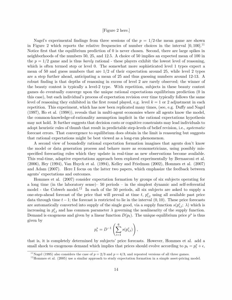
[Figure 2 here.]

Nagel’s experimental findings from three sessions of the p = 1/2-the mean game are shownin Figure 2 which reports the relative frequencies of number choices in the interval [0, 100].11

Notice first that the equilibrium prediction of 0 is never chosen. Second, there are large spikes inneighborhoods of the numbers 50, 25, and 12.5. A choice of 50 implies an expected mean of 100 inthe p = 1/2 game and is thus barely rational - these players exhibit the lowest level of reasoning,which is often termed step or level 0. The somewhat more sophisticated level 1 types expect amean of 50 and guess numbers that are 1/2 of their expectation around 25, while level 2 typesare a step further ahead, anticipating a mean of 25 and thus guessing numbers around 12-13. Arobust finding is that depths of reasoning in excess of level 2 are rarely observed; the winner ofthe beauty contest is typically a level-2 type. With repetition, subjects in these beauty contestgames do eventually converge upon the unique rational expectations equilibrium prediction (0 inthis case), but each individual’s process of expectation revision over time typically follows the samelevel of reasoning they exhibited in the first round played, e.g. level k = 1 or 2 adjustment in eachrepetition. This experiment, which has now been replicated many times, (see, e.g. Duffy and Nagel(1997), Ho et al. (1998)), reveals that in multi-agent economies where all agents know the model,the common-knowledge-of-rationality assumption implicit in the rational expectations hypothesismay not hold. It further suggests that decision costs or cognitive constraints may lead individuals toadopt heuristic rules of thumb that result in predictable step-levels of belief revision, i.e., systematicforecast errors. That convergence to equilibrium does obtain in the limit is reassuring but suggeststhat rational expectations might be best viewed as a long-run phenomenon.

A second view of boundedly rational expectation formation imagines that agents don’t knowthe model or data generation process and behave more as econometricians, using possibly mis-specified forecasting rules which they update in real-time as new observations become available.This real-time, adaptive expectations approach been explored experimentally by Bernasconi et al.(2006), Hey (1994), Van Huyck et al. (1994), Kelley and Friedman (2002), Hommes et al. (2007)and Adam (2007). Here I focus on the latter two papers, which emphasize the feedback betweenagents’ expectations and outcomes.

Hommes et al. (2007) consider expectation formation by groups of six subjects operating fora long time (in the laboratory sense)— 50 periods — in the simplest dynamic and self-referentialmodel - the Cobweb model.12 In each of the 50 periods, all six subjects are asked to supply aone-step-ahead forecast of the price that will prevail at time t, pei,t using all available past pricedata through time t− 1; the forecast is restricted to lie in the interval (0, 10). These price forecastsare automatically converted into supply of the single good, via a supply function s(pei,t; λ) which isincreasing in pei,t and has common parameter λ governing the nonlinearity of the supply function.Demand is exogenous and given by a linear function D(pt). The unique equilibrium price p∗ is thusgiven by

p∗t = D−1Ã

6Xi=1

s(pei,t)

!,

that is, it is completely determined by subjects’ price forecasts. However, Hommes et al. add asmall shock to exogenous demand which implies that prices should evolve according to pt = p∗t + ,

11Nagel (1995) also considers the case of p = 2/3 and p = 4/3, and repeated versions of all three games.12Hommes et al. (2005) use a similar approach to study expectation formation in a simple asset-pricing model.

14

where ∼ N(0, σ2). Thus under rational expectations, all forecasters should forecast the sameprice, p∗. In the new learning view of rational expectations, it is sufficient that agents have accessto the entire past history of prices for learning of the rational expectations solution to take place.Consistent with this view, Hommes et al. do not inform subjects of the market clearing processby which prices are determined. Instead, subjects are simply engaged in forming accurate priceforecasts and individual payoffs are a linearly decreasing function of the quadratic loss (pt − pei,t)

2.The main treatment variable consists of variation in the supply function parameter λ which affectsthe stability of the cobweb model under the assumption of naive expectations (following the classicanalysis of Ezekiel (1938)). The authors consider three values for λ for which the equilibrium isstable, unstable or strongly unstable under naive expectations.13 Their assessment of the validity ofthe rational expectations assumption is based on whether market prices are biased (looking at themean), whether price fluctuations exhibit excess volatility (looking at the variance) and whetherrealized prices are predictable (looking at the autocorrelations).

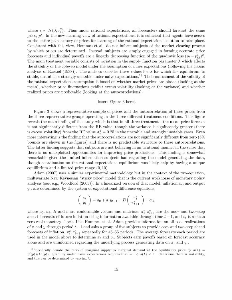
[Insert Figure 3 here].

Figure 3 shows a representative sample of prices and the autocorrelation of these prices fromthe three representative groups operating in the three different treatment conditions. This figurereveals the main finding of the study which is that in all three treatments, the mean price forecastis not significantly different from the RE value, though the variance is significantly greater (thereis excess volatility) from the RE value σ2 = 0.25 in the unstable and strongly unstable cases. Evenmore interesting is the finding that the autocorrelations are not significantly different from zero (5%bounds are shown in the figures) and there is no predictable structure to these autocorrelations.The latter finding suggests that subjects are not behaving in an irrational manner in the sense thatthere is no unexploited opportunities for improving price predictions. This finding is somewhatremarkable given the limited information subjects had regarding the model generating the data,though coordination on the rational expectations equilibrium was likely help by having a uniqueequilibrium and a limited price range (0, 10)

Adam (2007) uses a similar experimental methodology but in the context of the two-equation,multivariate New Keynesian “sticky price” model that is the current workhorse of monetary policyanalysis (see, e.g., Woodford (2003)). In a linearized version of that model, inflation πt, and outputyt, are determined by the system of expectational difference equations,µ

πtyt

¶= a0 + a1yt−1 +B

µπetπet+1

¶+ cvt

where a0, a1, B and c are conformable vectors and matrices, πet πet+1 are the one— and two—stepahead forecasts of future inflation using information available through time t− 1, and vt is a meanzero real monetary shock. Like Hommes et al. Adam provides information on all past realizationsof π and y through period t−1 and asks a group of five subjects to provide one- and two-step aheadforecasts of inflation, πet π

et+1 repeatedly for 45—55 periods. The average forecasts each period are

used in the model above to determine πt and yt. Subjects earn payoffs based on forecast accuracyalone and are uninformed regarding the underlying process generating data on πt and yt.

13Specifically denote the ratio of marginal supply to marginal demand at the equilibrium price by σ(λ) =S0(p∗t )/D

0(p∗t ). Stability under naive expectations requires that −1 < σ(λ) < 1. Otherwise there is instability,and this can be determined by varying λ.

15

The rational expectation solution is of the form:

yt = y + vt

πt = (π/y)yt−1

where y and π represent steady state values. Inflation lags output by one period due to pre-determined (sticky) prices, and output deviates from its steady state only due to real monetaryshocks. Thus a rational forecast model for πt should condition on yt−1, i.e. πt = αy + βyyt−1.Of course, since subjects are given time series data on both y and π, Adam imagines that sub-jects might alternatively use a simple (but miss-specified) autoregressive forecast model of the formπt = απ + βππt−1. Thus, the issue being tested here is not simply one of whether agents canlearn to form rational expectations of future inflation but more importantly whether subjects, likeeconometricians, can find the correct specification of the reduced form model they should use toform those rational expectations. Perhaps not surprisingly, the evidence on the latter question issomewhat mixed. Adam finds that in most of the experimental sessions, subjects forecast usingthe autoregressive inflation model and do not condition their forecasts on lagged output. However,he also shows that such behavior can result in a stationary, “restricted perceptions” equilibriumthat is optimal in the sense that autoregressive inflation forecasts outperforms those that conditionon lagged output. Adams further notes that this miss-specification in agents forecasts providesa further source of inflation and output persistence in addition to that implied by the model’sassumption of sticky price adjustment.

Summing up, we have seen some ways in which three micro-level assumptions that are mainstaysof macroeconomic modeling - intertemporal optimization, time-consistent preferences/exponentialdiscounting and the rationality of expectations have been tested in the laboratory, primarily inindividual decision-making experiments. The evidence to date suggests that human subject behav-ior is often at odds with the standard micro-assumptions of macroeconomic models. The behaviorof subjects appears to be closest to micro-assumptions, e.g., intertemporal optimization, whensubjects learn from one another or gather information on prices through participation in markets.Rational expectations appears to be most reasonable in simple, univariate models (e.g. the Cobwebmodel) as opposed to the more commonly used multivariate models. Hopefully these and otherexperimental findings will lead to a reconsideration of the manner in which macroeconomic mod-elers characterize the behavior of their “representative” agents, though so far, there is not muchevidence that such a change is imminent.

3 Coordination Problems

In the previous section, we focused on individual behavior in dynamic intertemporal optimizationproblems where the optimal, rational expectations solution was unique. In many macroeconomicenvironments, this is not the case. Instead, multiple rational expectations equilibria exist and thequestion is which of these equilibria economic agents will choose to coordinate upon. Laboratoryexperiments can be quite useful in this regard. Indeed, Lucas (1986) argued that laboratory ex-periments were a reasonable means of resolving such coordination problems, because “economictheory does not resolve the situation [so] it is hard to see what can advance the discussion short ofassembling a collection of people, putting them in the situation of interest, and seeing what theydo.”

16

Some coordination problems of interest to macroeconomists were previously addressed in Ochs(1995). In particular, that chapter surveyed experimental studies of overlapping generations modelswhere money may or may not serve as a store of value (Lim et al. (1994)), or subjects can selectbetween low or high inflation equilibria (Marimon and Sunder (1993, 1994, 1995)). Also includedwere experimental studies of stag-hunt and battle—of—the sexes games (surveyed also in Cooper1999) and Bryant (1983)-type Keynesian coordination games (e.g., the minimum and median effortgames of Van Huyck 1990, 1991, 1994).14 The coordination games literature delivered a number ofimportant findings on when coordination success was likely to be achieved and when coordinationfailure was likely. Importantly, the results have been replicated by many other experimenters lead-ing to confidence in those findings. Rather than review those replications and extensions, in thissection I report on more recent macro-coordination experiments. The environments tested in theseexperiments have a more direct resemblance to macroeconomic models than do the coordinationgames surveyed by Ochs, (with the exception of Marimon and Sunder’s work on overlapping gen-erations models). I also address some equilibrium selection mechanisms or refinements that havebeen proposed for resolving macro-coordination problems and the experimental studies of thosemechanisms and refinements.

3.1 Poverty Traps

Lei and Noussair (2007) build on their (2002) experimental design for studying behavior in the one-sector optimal growth model by adding a non-convexity to the production technology, resulting inmultiple, Pareto-rankable equilibria. Specifically, the production function used to determine outputin Matheny and Noussair (2000) and Lei and Noussair (2002) is changed to:

f(kt) =

½Akαt if kt < k∗

Akαt if kt ≥ k∗.

where A < A and k∗ is a threshold level of aggregate capital stock that is known to all 5 subjects.The threshold switch in productivity is a simple way of modeling positive externalities that mayarise once an economy reaches a certain stock of capital (physical or human) (see, e.g. Azariadisand Drazen (1990)). An implication is that there are now two stationary levels for the capitalstock (and output) kl < k∗ < kh, with kl representing the poverty trap and kh representing thePareto efficient equilibrium. The dynamics of the system (under perfect foresight) are such thatfor k ∈ (0, k∗), kl is an attractor whereas for k ≥ k∗, kh is the attractor. The main experimentalquestion is which of these two equilibria subjects while learn to coordinate on.

One treatment variable was the initial aggregate level of the capital stock, either below or abovethe threshold level k∗ and divided up equally among the 5 subjects. The other treatment conditionwas whether decisions were made in a decentralized fashion, with a market for the capital stock(subjects had different production technologies that aggregated up to the aggregate technology) orwhether groups of subjects together made a collective consumption-savings decision, i.e. playingthe role of a social planner. In both cases, the indefinite horizon of the model was implementedusing a constant probability of continuation and subjects were paid on the basis of the utility valueof the consumption they were able to achieve in each period. The main experimental finding is thatin the decentralized treatment, the poverty-trap equilibrium is a powerful attractor; it is selected14That material, while highly relevant to the literature on experimental macroeconomics will not be repeated here

— the interested reader is referred to Ochs (1995). See also Camerer (2003 chp. 7) and Devetag and Ortmann (2007)

17

in all sessions where the initial aggregate capital stock is below k∗ as well as in some sessions wherethe initial aggregate capital stock lies above k∗. There are some instances of convergence to thePareto efficient stationary equilibrium kh, but only in the decentralized setting where the initialcapital stock lies above k∗. In the social planner treatment, where 5-subject groups jointly decide onconsumption-savings decisions, neither of the two stationary equilibria were ever achieved; insteadthere was either convergence to a capital stock close to the threshold level k∗, or to the golden-rulelevel that maximally equates consumption in every period. While the latter is close to the Paretooptimum it is inefficient, as it ignores the possibility that the economy may terminate (the rate oftime preference is positive). Lei and Noussair (2007) conclude that additional institutional featuresmay be necessary to both avoid and escape from the poverty trap outcome.

The possibility that various institutional mechanisms might enable economies to escape povertytraps is taken up in a follow-up experimental study by Capra et al. (2005). These authors begin bynoting that laboratory studies of the role of institutions in economic growth may avoid endogeneityproblems encountered in field data studies (where it is unclear whether institutions cause growth orvice versa), and more clearly explore environments with multiple institutions. The two institutionsexplored in this study are termed “freedom of expression,” which involves free discussion amongsubjects prior to each round of decision-making and “democratic voting” in which subjects voteon two proposals for how to divide output up between consumption and savings (future capital) atthe end of each period.

The baseline experimental design is essentially the same as the low initial capital stock treatmentof Lei and Noussair (2007); there are five subjects who begin each indefinite sequence of roundswith capital stocks that sum up to an aggregate level that lies below the threshold level k∗.15 Thisinitial condition for the aggregate capital stock is the same in all treatments of this study, as thefocus here is on whether subjects can escape from the poverty trap equilibrium. At the start of aperiod, output is produced based on last period’s capital stock and then a market for capital (theoutput good opens). After the market for capital has closed, subjects independently and withoutcommunication decide on how to allocate their output between current consumption and savings(next period’s capital stock). In the communication treatment, subjects are free to communicatewith one another prior to the opening of the market for capital. In the voting treatment, after thecapital market has closed, two subjects are randomly selected to propose consumption/savings plansfor all five agents in the economy; these proposals specify how much each subject is to consume andhow much to invest in next period’s capital stock (if there is a next period). Then all five subjectsvote on the proposal they prefer and the proposal winning a majority of votes is implemented. Ina hybrid treatment, both communication and voting stages are included together.

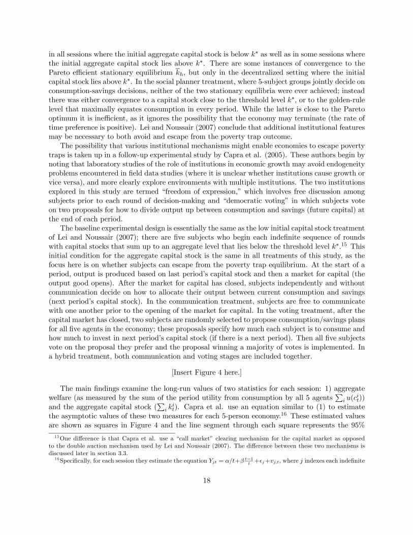
[Insert Figure 4 here.]

The main findings examine the long-run values of two statistics for each session: 1) aggregatewelfare (as measured by the sum of the period utility from consumption by all 5 agents

Pi u(c

it))

and the aggregate capital stock (P

i kit). Capra et al. use an equation similar to (1) to estimate

the asymptotic values of these two measures for each 5-person economy.16 These estimated valuesare shown as squares in Figure 4 and the line segment through each square represents the 95%15One difference is that Capra et al. use a “call market” clearing mechanism for the capital market as opposed

to the double auction mechanism used by Lei and Noussair (2007). The difference between these two mechanisms isdiscussed later in section 3.3.16Specifically, for each session they estimate the equation Yjt = α/t+β t−1

t+ j+vj,t, where j indexes each indefinite

18

confidence region. The lower left intersection of the dashed lines shows the poverty trap level ofaggregate welfare and capital, while the upper right intersection of the two dashed lines shows thePareto efficient level of aggregate welfare and capital. This Figure reveals the main findings In thebaseline treatment, consistent with Lei and Noussair, subjects are unable to escape from the povertytrap outcome. The addition of communication or voting helps some, though not all economies toescape from the poverty trap. In the hybrid model which allows both communication and voting,the experimental economies appear to always escape from the poverty trap (95% confidence boundsexclude poverty trap levels) and these economies are closest to the Pareto efficient equilibrium levelsfor welfare and the capital stock. Capra et al. argue that binding consumption/savings plans asin the voting treatment are important for achieving aggregate capital stock levels in excess of thethreshold level, while communication makes it more likely that such consumption/savings plans areconsidered in the first place; not surprisingly then, the two institutions complement one anotherwell and lead to the best outcomes.

While this experimental design involves a highly stylized view of the institutions labeled “free-dom of expression” and “democratic voting” the same critique can be made of the neoclassicalmodel of economic growth. The experimental findings suggest that there may be some causalityfrom the existence of these institutions to the achievement of higher levels of capital and welfare,though the opposite direction of causality from growth to institutions remains an important possi-bility. More recently, macroeconomists have emphasized the role of human capital accumulation,so it would be of interest to consider whether subjects learn to exploit a positive externality from ahighly educated workforce). And while several other studies have pointed to the usefulness of com-munication in overcoming coordination problems (see, e.g., Blume and Ortmann (2007), Cooper etal. (1992), these have been in the context of strategic form games. While the results of those studiesare often cleaner, in the sense that the game is simple and communication is highly scripted, theCapra et al. study implements institutional features in a model that macroeconomists care aboutand this may serve to improve the nascent dialogue between experimentalists and macroeconomists.

3.2 Bank Runs

Another coordination problem that has been studied experimentally in the context of a model thatmacroeconomists care about is Diamond and Dybvig’s (1983) coordination game model of bankruns. In this three period intertemporal model, depositors find it optimal to deposit their unitendowment in a bank in period 0, given the bank’s exclusive access to a long-term investment op-portunity and the deposit contract the bank offers. This deposit contract provides depositors withinsurance against uncertain liquidity shocks; in period 1, some fraction learn they are have imme-diate liquidity needs (are impatient) and must withdraw their deposit early, while the remainingfraction learn they are patient and can wait to withdraw their deposit in the final period 2. Thebank uses its knowledge of these fractions in optimally deriving the deposit contract, which stipu-lates that depositors may withdraw the whole of their unit endowment at date 1 while those whowait to withdraw until period 2 can earn R > 1. While there exists a separating, Pareto efficientequilibrium where impatient types withdraw early and patient types wait until the final period,there also exists an inefficient pooling equilibrium where uncertainty about the behavior of other

sequence or “horizon” within a session. The dependent variable Yj,t is either aggregate welfare, U(ct) =5i=1 ui(c

it)

or the aggregate capital stock kit =5i=1 k

it. The two asymptotic estimates for each session —the estimates of β for

each of the two dependent variables — are the squares shown in Figure 4.

19

Hypothetical Amount Each ProjectedNo. of Withdrawl Requester Payment to

Requests Would Receive Each Depositor0 n/a $1.501 $1 $1.502 $1 $1.503 $1 $04 $0.75 $05 $0.60 n/a

Table 2: Bank-Run Coordination Game Payoffs, Garratt and Keister (2005)

patient types causes all patient types to mimic the impatient types and withdraw their depositsin period 1 rather than waiting until period 2. In the latter case, the bank has to liquidate itslong-term investment in period 1 and depending on the liquidation value of this investment, it mayhave insufficient funds to honor its deposit contract in period 1. The possibility of this bank-runequilibrium is the focus of experimental studies by Garratt and Keister (2005) and Schotter andYorulmazer (2003).

Garratt and Keister’s baseline experimental design dispenses with controlling for the two typesand focuses on the pure coordination game aspect of the problem. Five subjects have $1 depositedin a bank and must decide at one or more opportunities whether to withdraw their $1 or leaveit deposited in the bank potentially earning a higher return of $1.50. Following each withdrawalopportunity, subjects learn the number of players in their group of 5 (if any) who have chosen towithdraw. As treatment variables, Garratt and Keister varied the number of withdrawal opportu-nities (1 or 3) and the number of early withdrawals a bank could sustain while continuing to offerthose who avoided withdrawal a payoff of $1.50 (i.e. variation in the liquidation value of the bank’slong-term investment). Table 2 provides one parameterizations of Garratt and Keister’s bank-rungame.

Garratt and Keister report that for this baseline game, regardless of the liquidation value of thelong-term investment, no group ever coordinated on the “panic equilibrium” (5 withdrawals) anda majority of groups coordinated on the payoff dominant equilibrium (0 withdrawals). In a secondtreatment that more closely implements the liquidity shock in the Diamond-Dybvig model, Garrattand Keister added “forced withdrawals” to the baseline game: at each withdrawal opportunity,there was a small known probability that one randomly selected player would be forced to withdraw;however whether a withdrawal was forced or not was unknown to subjects. The probabilities offorced withdrawals were chosen such that there continued to exist a payoff dominant equilibriumin which no player ever voluntarily withdrew at any withdrawal opportunity (if all adhered tothis strategy they would earn an expected payoff greater than $1) as well as a panic equilibriumwhere all withdraw. Garratt and Keister report that with forced withdrawals (liquidity shocks) thefrequency of voluntary withdrawals and coordination on the panic equilibrium is significantly greaterrelative to the baseline treatment with unforced withdrawals. This increase in panic behavior wasparticularly pronounced in the forced withdrawal treatment where subjects had multiple withdrawalopportunities and could condition their decisions on the prior decisions of others. An implication

20

of this finding is that panic behavior may require some conditioning on the decisions of otherssuggesting that the bank run phenomenon is perhaps best modeled as a dynamic game, as opposedto the simultaneous-move formulation of Diamond and Dybvig (1983).

Schotter and Yorulmazer (2003) arrive at a similar conclusion, using a rather different experi-mental design. Theirs involves a group of six subjects deciding in which of four periods to withdrawtheir deposit of $K in the face of uncertainty concerning both the withdrawal decisions of the otherfive subjects as well as the type of bank that all 6 have invested their deposits in. Subjects knowthat there are 5 possible bank types, that each type is equally likely to be drawn for the durationof each 4-period game, and that the mean return across types is r∗.17 While the bank type isunobservable, the “promised” return is fixed at 12% per period, while the mean return r∗ wasvaried across sessions, either .07, .08 or .14. Subjects were told that if they kept their $K depositinvested for periods, they could earn a return of $(1.12) K if the bank has sufficient funds leftin period , but if not, the bank would pay all those withdrawing in that period an equal share ofremaining funds on hand (if any). Subjects had to choose in which of the four periods to with-draw their money, with withdrawal being irreversible. The authors think of this as a model of abank—run—in—progress, (the precipitating event is left unmodeled) and are interested in exploringthree factors that may slow or hasten the period in which deposits are withdrawn. A first factoris whether the withdrawal decision across the four periods is implemented as a simultaneous-movenormal form game, or as an extensive form game; in the former case subjects specify the periodin which they want to withdraw their funds (1,2,3,or 4) while in the latter case subjects makewithdrawal decisions period by period and may condition on the prior period withdrawal decisions(and in one treatment, the amounts earned) by others. The second and third factors are the useof deposit insurance to delay or slow down the run or the presence of insiders who know the meanreturn r∗ of the banks, and may through their actions persuade other uniformed subjects to runearly or wait.

Schotter and Yorulmazer find that bank runs are less likely to be severe (withdrawal occurslater, e.g. in period 3 or 4) when r∗ is known to be greater than the promised return of 12%. Forfixed r∗, runs are also less severe in the extensive form version of their model, when agents cancondition on the decisions of others and there is a high degree of information, in that subjects alsoknow the amounts that others have received.18 This finding is interesting in that theory does notpredict that the game form should matter; the fact that it does again points to the value of thinkingof bank runs as dynamic rather than static games. They further show that partial deposit insurancemay work to diminish the severity of bank runs as can the presence of some depositor—insiders whoknow the type of bank with which funds have been invested.

The issue of the contagious spread of a bank run from one location to another is addressedexperimentally by Corbae and Duffy (2008). They study a two stage, 4-player game. In the firststage, players simultaneously propose to form links with one another; mutually agreeable links arethen implemented and comprise the set of each player’s ‘neighbors’. Corbae and Duffy interpretthe players as ‘banks’ connected to one another via interbank reserve deposits that can serve toinsure against risk. (a la Allen and Gale (2000)). In the second stage, each player plays τ roundsof an n-person, equal-weighted- payoff stag hunt game with his n=1,2 or 3 neighbors. As in Garratt

17The possible returns from the five banks are known to belong to the set: {(1/3)r∗, (2/3)r∗, r∗, (4/3)r∗, (5/3)r∗}.18The latter finding may seem at odds with Garratt and Keister’s findings but note that Schotter and Yorulmazer

don’t have forced shocks, so their set-up is closest to Garratt and Keister’s setting without forced shocks, in whichpanics were rarely observed.

21

and Keister (2005), one of the 4-players is “shocked” i.e., randomly to play the inefficient ‘hare’or run strategy in all rounds of the second-stage game. Corbae and Duffy define a contagion asa movement by all players away from the Pareto efficient ’stag’ equilibrium to the inefficient hareequilibrium. While it is possible for subjects to implement a complete network of links (each ofthe 4 players has 3 links each) that provides insurance against the risk of being linked to playerforced to panic as when all unshocked players play ‘stag’, Corbae and Duffy show that such anetwork configuration is not an equilibrium due to the free-rider problem. Instead, the networkconfigurations that are predicted to emerge are bilateral networks (2-player networks where eachplayer has a single link) which serves to limit the spread of the bank run outcome. Corbae and Duffyreport experimental evidence that is broadly consistent with this prediction. Starting groups of 4subjects out in different exogenous network configurations and then in subsequent games allowingthem to choose the players they want to link to, they report that subjects consistently move in thedirection of choosing to have a single link to one other player. Under this bilateral network, thebank-run equilibrium is isolated to just one of the 2-player networks; the other network achievesthe efficient, payoff dominant equilibrium.

Summing up, we have discussed two kinds of macroeconomic-coordination experiments, povertytraps and bank runs. In the poverty trap model, the question of interest is how to get subjectsto move from an inefficient equilibrium to an efficient one. We might think of this as a goodcontagion. In the bank run model the question of interest is precisely the opposite - how to keepfunds deposited in a bank longer (earning higher returns) and avoiding a bad contagion to aninefficient panic equilibrium. Both types of movements are difficult to achieve in the laboratory.In the case of movement from an efficient to an inefficient equilibrium it seems necessary to forcesome players’ hands in order to precipitate a transition to the inefficient outcome; that findingsuggests that the precise mechanism precipitating a bad contagion has yet to be discovered.

We next explore experimental tests of two mechanisms that macroeconomists have used toresolve coordination problems.

3.3 Resolving Coordination Problems: Sunspots

In the bank-run coordination game, the question of equilibrium selection is left unmodeled. Dia-mond and Dybvig (1983) suggest that depositors might use realizations of some commonly observed,non-fundamental random variable, or “sunspot” in the language of Cass and Shell (1983) and Azari-adis (1981) to resolve the question of which equilibrium to coordinate on.19 Experimental tests ofsunspot variables as coordination devices have been conducted by Marimon et al. (1993) and Duffyand Fisher (2005).20

Marimon and Sunder (1993) implemented a 2-period overlapping generations environmentwhere, if agents have perfect foresight, there are multiple equilibrium: an interior steady stateand a two-period cyclic equilibrium. Subjects in the role of young agents formed price expecta-

19John Maynard Keynes talked about “animal spirits” as a source of investment volatility. Charles McKay talkedabout the “madness of crowds” in documenting famous financial fiascos. These are references to the role played bynon-fundamental factors or “sunspots” in economic activity. The term “sunspot” derives from the work of WilliamStanley Jevons, a nineteenth century economist and polymath who championed the notion that the solar cycle wasresponsible for the business cycle. Of course, business cycles are a lot more irregular than the 11-year sunspot cycleand there is considerable variation in the timing and duration of business cycles across countries. So today, we honorJevon’s folly by referring to non-fundamental or extraneous factors that may affect business activity as “sunspots”.20Here I emphasize the latter study, as the Marimon et al. (1993) study is thoroughly discussed in Ochs (1995).

22

tions which determined current prices, given the nonlinear model, pt = φ(pet+1). Thus given priceexpectations, subjects optimal consumption and savings in the form of real money balances wasdetermined (as in Marimon and Sunder (1993, 1994). Marimon and Sunder hoped that subjectswould use realizations of a sunspot variable to coordinate their expectations on the cyclic equi-librium. Their sunspot variable consisted of a blinking cube on subjects’ computer screens. Thecolor of this cube alternated every period between red and yellow. Marimon and Sunder found thatsubjects essentially ignored the sunspot variable realizations and simply coordinated on the steadystates. They later tried to add a correlation between the sunspot variable and a real endowmentshock (alternating the size of the young generation between 3 and 4 subjects, i.e., 3-4-3-4) but thisalso did not lead to coordination on the sunspot variable when the endowment shock was shut off.

Duffy and Fisher (2005) consider a simpler, partial equilibrium framework that abstracts froma number of conceptual difficulties (e.g. implementing an infinite horizon). In this simple andstatic environment there are two equilibria that differ only in terms of the equilibrium price level;the equilibrium quantity is the same in both. The experimental design involves 5 buyers and 5sellers, each with two units to buy or sell. Buyers seek to maximize consumer surplus, (valuation -price), while sellers seek to maximize producer’s surplus (price - cost). Further each buyer (seller)had two possible valuations (costs) for each of his two units. If the state was “high” each buyer’s(seller’s) profits were calculated using his two high valuations (costs). If the state was “low” eachbuyer’s (seller’s) profits were calculated using his two low valuations (costs). The two sets ofvaluations/costs used in the experiment are shown in Figure 5.

[Figure 5 here.]

Two market clearing mechanisms were considered - the standard double auction where bidsand asks can be observed in real-time and a sealed-bid variant known as a call-market, where bidsand asks are submitted simultaneously, bids are sorted from highest to lowest, asks from lowest tohighest and a single market clearing price is determined by the intersection of demand and supply(if there is one). All buyers (sellers) with bids (asks) above (below) the market price get to buy (sell)their units (provided there are enough units on both sides). The state of the world was determinedby the median traded price in the double auction or by the market clearing price in the call-market.If either was greater than or equal to 150, then the high state was declared and subjects uses highvaluations or costs in determining their surplus (payoff). Otherwise the low state was declared andlow valuations and costs were used in the determination of payoffs. Thus the situation is akin toone in which there are multiple equilibria, each supported by different beliefs about the likely stateof the world.

Duffy and Fisher’s sunspot variable was one of two possible announcements made prior to eachof 10 four-minute trading periods. The announcement chosen was determined by publicly flippinga coin. In one treatment, if the coin flip was heads, the public announcement was “the forecastis high” while if the coin flip was tails, the public announcement was “the forecast is low” andthis scheme was public knowledge. Duffy and Fisher report that in sessions using a call marketclearing mechanism, subjects perfectly coordinated on the high price equilibrium when the forecastwas high and on the low price equilibrium when the forecast was low - that is the sunspot variablewas shown to matter for economic volatility. On the other hand under the double auction marketclearing mechanism, the sunspot announcements only sometimes served to coordinate subjects onthe high or low equilibrium. Duffy and Fisher argue that the reason for this difference lies in thereal-time information that was available in the double-auction; subjects could see bids and asks

23

as they occurred and could use this fact to attempt to engineer an equilibrium outcome for prices(high or low) that was more favorable to them.21 Thus the coordinating mechanism provided bythe sunspot could be undone by the real-time information on bids, asks and trade prices. The samewas not possible in the call-market where bids and asks had to be submitted simultaneously andhence the sunspot variable played an important coordinating role in the environment.

Duffy and Fisher further show that the semantics of the sunspot variable matter: replacing theforecast is “high” or “low” with the forecast is “sunshine” or “rain” eliminated the sunspot variableas a coordinating mechanism in the call market. Further research might seek to understand howthe mapping from sunspot variable realizations to the action space matter in getting subjects tocoordinate on sunspot equilibria. It would also be of interest to consider sunspot equilibria thatare not simply randomizations over two certainty equilibria.

3.4 Resolving Coordination Problems: The Global Game Approach

Another view of multiple equilibria in macroeconomic modeling is that the equilibrium beliefs insupport of these equilibria may not be as indeterminate as theory supposes. As Morris and Shin(2001) argue, these indeterminacies arise from assuming that economic fundamentals are commonknowledge and that individuals are certain of the behavior of others in equilibrium. Relaxing theseassumptions, e.g. by introducing some uncertainty about fundamentals, can remove the multiplicity,á la the Carlsson and van Damme’s (1993) global game approach for 2× 2 games.22 The resultinggame is one in which individuals adopt a unique threshold strategy -when fundamentals are weak,individuals are pessimistic about others’ beliefs and the resulting outcome is poor, as in the bankrun equilibrium. However if fundamentals are strong so will be beliefs about others’ beliefs andthe resulting outcome will be good, as in a payoff dominant equilibrium. This correlation betweenfundamentals and outcomes is missing from the sunspot approach.23

Heinemann et al. (2004) conducted the first experimental test of the global game approach toresolving equilibrium multiplicity in the context of a speculative currency attack model developedby Obstfeld (1996) and Morris and Shin (1998). Prior to the start of each 2 × n player game, apayoff relevant random variable Y is drawn from a uniform distribution with known support. Thisvariable represents the fundamentals of the economy with higher (lower) values of Y representingworse (better) fundamentals. In the complete information (CI) treatment, this variable is known toall 15 subjects while in the private information (PI) treatment, the value of Y is not known but eachof the 15 subjects receives noisy signals of Y , Xi, that are uniform random draws from the knowninterval [Y − , Y + ] where is small. Subjects must then decide between two actions, A and B,where A is a safe choice resulting in a fixed payoff F (equivalent to not-running or not-attackinga currency). The other choice, B, is a risky choice (equivalent to attacking a currency, joining arebellion, etc.) the payoff from which depends on the total number of players who choose B, asdetermined by a monotonically decreasing function f(Y ). If less than f(Y ) agents choose B allthose choosing B earn 0 (the attack fails) while if at least f(Y ) agents choose B, then all those

21Notice from Figure 4 that 2 out of 5 buyers/sellers prefer the high equilibrium and 2 out of five prefer the lowequilibrium and the remaining buyer and seller are indifferent. Thus, the equilibria are not Pareto rankable.22 In Carlsson and van Damme’s approach, players facing a game of complete information with multiple equilibria

behave as though it were a perturbed global game of incomplete information where the payoffs are determined by arandom draw from a given class of games and players have a noisy signal of the chosen game.23There is some debate about whether bank runs and financial crises are caused by fundamental or non-fundamental

(sunspots).

24

choosing B earn Y points (the attack succeeds). Consistent with the theory, the distribution ofY values is chosen so that there exists values of Y ≤ F , for which it is a dominant strategy tochoose A and similarly there exist values of Y ≥ f−1(1) for which a single individual can guaranteethe success of an attack by choosing B, so that it is dominant for all to do so. For Y values in(F, f−1(1)), under complete information, there are multiple equilibria: all choose A or all chooseB, both of which can be supported by the belief that all others will choose A or B. However inthe incomplete information game there exists a unique, threshold value of the noisy signal X forwhich all subjects should attack (choose B) if their signal is above the threshold and not attackotherwise. Taking the limit as → 0 it is possible to find a similar threshold Y ∗ in the completeinformation game.

The main question pursued by Heinemann et al. is whether the complete information game,with its multiplicity of equilibria is more unstable than the private information game, and whethersubjects adopt threshold strategies consistent with the global game threshold prediction. Theyreport that subjects do appear to adopt threshold strategies in both the private and completeinformation cases and these estimated thresholds generally lie below the global game predictionsX∗ or Y ∗ but are higher than the payoff-dominant prediction of choosing B whenever Y > F . Themost interesting finding is in the complete information treatment, where Y is publicly known andthere are in principle multiple equilibria. In that treatment Heinemann et al report less variancein entry decisions than in the incomplete information treatment and greater coordination on acommon threshold in the former as compared with the latter. Heinemann et al conclude that“with public information the central bank has more control over trader’s beliefs than when theyget private information from other sources.”

The global game refinement has been further tested in several other experimental studies.Cabrales et al. (2007) test the theory in two-person games with a more discrete state space.They find greater coordination on the global game prediction in the incomplete information caseand on the payoff dominant equilibrium in the complete information case. Duffy and Ochs (2008)embedded Heinemann et al.’s design in a dynamic setting where subjects have multiple periods inwhich to decide whether to attack or not and may condition their decision on the prior decisions ofothers. They report little difference in the thresholds used in the dynamic game as compared withthose used in the static game. Cornand (2006) adds two treatments, one with a private signal and apublic signal and a second with two noisy public signals. She reports that subjects overreact to thepublic signal when they also receive a private one, but that predictability of an attack is higher inthat case as compared to the case of two noisy public signals. This finding suggests that if officialsare going to make public amusements they would do well to coordinate on a single message.

Summarizing, we have considered laboratory evidence on several mechanisms for selecting fromamong multiple equilibria in macroeconomic models including communication, voting, sunspots andthreshold strategies based on the global game refinement. The laboratory is a natural testing groundfor these mechanisms as other confounding factors can be minimized and attention can be focusedon the hypothesized coordination device (perhaps too ideal a setting?) The experimental findingsto date suggest mixed support for any single mechanism as the means by which individuals actuallygo about solving coordination problems. Still, many improvements on these studies remain to beconducted and it is likely that with further study we will have a better sense of which mechanismswork best in particular settings.

25

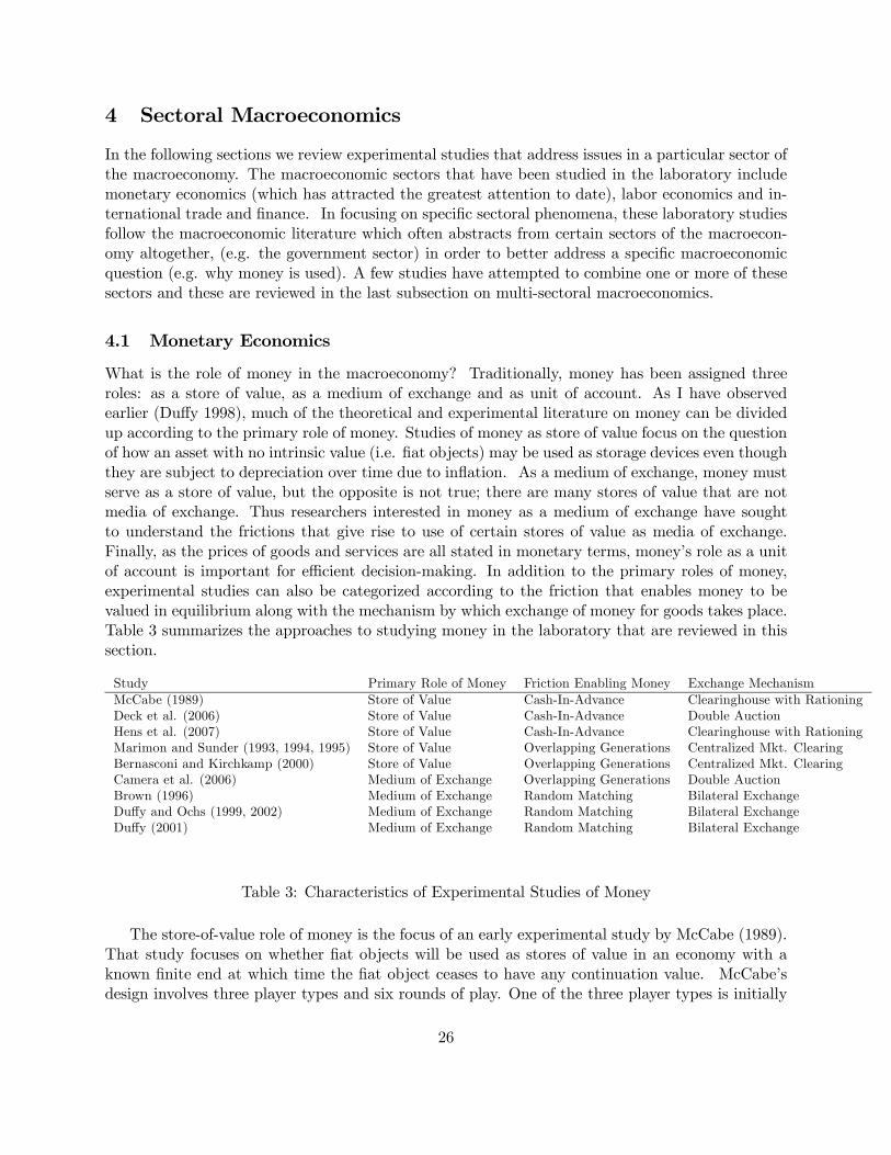
4 Sectoral Macroeconomics

In the following sections we review experimental studies that address issues in a particular sector ofthe macroeconomy. The macroeconomic sectors that have been studied in the laboratory includemonetary economics (which has attracted the greatest attention to date), labor economics and in-ternational trade and finance. In focusing on specific sectoral phenomena, these laboratory studiesfollow the macroeconomic literature which often abstracts from certain sectors of the macroecon-omy altogether, (e.g. the government sector) in order to better address a specific macroeconomicquestion (e.g. why money is used). A few studies have attempted to combine one or more of thesesectors and these are reviewed in the last subsection on multi-sectoral macroeconomics.

4.1 Monetary Economics

What is the role of money in the macroeconomy? Traditionally, money has been assigned threeroles: as a store of value, as a medium of exchange and as unit of account. As I have observedearlier (Duffy 1998), much of the theoretical and experimental literature on money can be dividedup according to the primary role of money. Studies of money as store of value focus on the questionof how an asset with no intrinsic value (i.e. fiat objects) may be used as storage devices even thoughthey are subject to depreciation over time due to inflation. As a medium of exchange, money mustserve as a store of value, but the opposite is not true; there are many stores of value that are notmedia of exchange. Thus researchers interested in money as a medium of exchange have soughtto understand the frictions that give rise to use of certain stores of value as media of exchange.Finally, as the prices of goods and services are all stated in monetary terms, money’s role as a unitof account is important for efficient decision-making. In addition to the primary roles of money,experimental studies can also be categorized according to the friction that enables money to bevalued in equilibrium along with the mechanism by which exchange of money for goods takes place.Table 3 summarizes the approaches to studying money in the laboratory that are reviewed in thissection.

Study Primary Role of Money Friction Enabling Money Exchange MechanismMcCabe (1989) Store of Value Cash-In-Advance Clearinghouse with RationingDeck et al. (2006) Store of Value Cash-In-Advance Double AuctionHens et al. (2007) Store of Value Cash-In-Advance Clearinghouse with RationingMarimon and Sunder (1993, 1994, 1995) Store of Value Overlapping Generations Centralized Mkt. ClearingBernasconi and Kirchkamp (2000) Store of Value Overlapping Generations Centralized Mkt. ClearingCamera et al. (2006) Medium of Exchange Overlapping Generations Double AuctionBrown (1996) Medium of Exchange Random Matching Bilateral ExchangeDuffy and Ochs (1999, 2002) Medium of Exchange Random Matching Bilateral ExchangeDuffy (2001) Medium of Exchange Random Matching Bilateral Exchange

Table 3: Characteristics of Experimental Studies of Money

The store-of-value role of money is the focus of an early experimental study by McCabe (1989).That study focuses on whether fiat objects will be used as stores of value in an economy with aknown finite end at which time the fiat object ceases to have any continuation value. McCabe’sdesign involves three player types and six rounds of play. One of the three player types is initially

26

endowed with a durable ticket (fiat money) that can be exchanged for one unit of any good andthe other two types are endowed with nondurable goods. Exchanges of tickets for goods occurs viaa centralized clearinghouse with known rationing rules; barter exchanges of goods for goods arenot allowed, so effectively a cash-in-advance constraint operates. Holding a good at the end of around yields different redemption values to different player types (either $0.50, $0.25 or $0.0) andthe endowments of these goods also varies across player types. If this game continued withoutend, the use of tickets would enable the efficient exchange of goods to types who most value thosegoods (direct barter is ruled out). However, since the game is known to have a finite end at whichpoint tickets have zero value, via a backward induction argument, tickets should never be acceptedin trade. McCabe however reports that tickets are indeed accepted, though with some fall-off nearthe end of each six round game. Despite repeating the six-round game 10-20 times with the samegroup of subjects, tickets continue to circulate in early rounds of the game. McCabe did eventuallysucceed in eliminating all trade in tickets but only after bringing back the same group of subjectsfor two further sessions, each a week apart. McCabe suggests that the inexperienced subjects’ useof tickets may be sustained by strong home-grown prior beliefs that money-type objects such astickets will be accepted in exchange as they are in everyday life.

[Figure 6 here].

Deck et al. (2006) follow up on the McCabe study by adding government agents who, unlike theother two player types in their study, are not budget constrained as to the quantity of tickets theycan redeem for goods (i.e. they can “print money”). The two other player types, "A" and "B", areendowed each period with amounts of goods B and A respectively, but profit from acquiring certainamounts of goods A and B respectively; unlike the government player types, the A and B-typeplayers are liquidity-constrained and must resort to trading the good they are endowed with inthe two double-auction goods market for tickets in order to buy the good they desire to consume.Figure 6 provides an illustration. As barter is disallowed, the friction giving rise to a demandfor money is a cash-in-advance constraint. As in McCabe’s study, there is a finite horizon which isvaried and in some treatments where money is "backed", tickets have a final cash redemption value.In treatments without government agents, subjects use money as a store of value (and hence as amedium of exchange) regardless of whether it is backed or not and despite the finite horizon as inMcCabe (1989). The addition of the government agents who are not budget constrained and whodesire additional units of both goods leads to a rapid escalation of the price level, which Deck et al.term a hyperinflation. This outcome arises in part because the government agents’ ability to printtickets leads to a rapid increase in the supply of money but Deck et al. emphasize that the erraticmeans by which the government introduces newly printed money augments the corruption of theinformation revealed in market traded prices. The hyperinflation finding is consistent with thework of Sargent (1983) who attributes historical episodes of hyperinflations to excessive fiat moneycreation. Deck (2004) provides further experimental evidence that hyperinflations of the Deck et al.(2006) variety can be ended by either making the currency convertible or by limiting governmentspending to current tax receipts (a balanced budget). Such mechanisms are also consistent withthe historical record on ending hyperinflations.

Similar to the Deck et al. study, Hens et al. (2007) address whether a fiat object can achievea stable value, facilitating its use as a medium of exchange. However, their focus is on whetheran optimal quantity of fiat money can be achieved. They present a model inspired by the CapitolHill Baby Sitting Co-op, a natural experiment in the 1970s in which approximately 150 Capitol

27

Hill couples exchanged baby-sitting duties with one another for coupons (Sweeny and Sweeny(1977)). The co-op organizers found that too few coupons led to coupon hoarding (precautionarysavings?) resulting in low demand for baby-sitting and a collapse of the system. An increase incoupons led to a thriving exchange of baby-sitting services, but eventually, over-issue of couponsresulted in excess demand for baby-sitting, and, given the fixed price of 1 coupon=1/2 hour ofbaby-sitting, led again to a collapse of the system. Hens et al. first develop a model whereinindividuals face preference shocks for a perishable single good (they have either a high or low valuefor it) eliminating barter, and must choose whether to be buyers/sellers of the good in each period.Buy or sell decisions are made simultaneously via a centralized mechanism with a long-side of themarket rationing rule. To buy a good, an individual must have money on hand, so a cash-in-advanceconstraint gives money value. Sales of goods augment an individual’s money holdings; prices arefixed. The unique equilibrium prediction of their rational expectations, forward looking, infinitehorizon model is that subjects who hold no money always offer to sell goods for money, regardlessof their period valuation for the good. Whether subjects choose to buy goods using money dependson their period valuation for the good. In the high valuation state, exchanging money for goodsis a dominant strategy. However, in the low valuation state, subjects should use money to buygoods only if their money holdings are sufficiently high; if below a critical level m, subjects shouldsell goods to acquire more money. This critical level of money holdings is related to the supply ofmoney, which is exogenously chosen. Hens et al. show that there is a unique optimal quantity ofmoney that maximizes the number of trades possible (i.e. no trader is rationed), given that playersare playing according to the optimal buy/sell strategy. The nicely designed experiment tests thesepredictions in a two stages. In the first stage subjects participate in individual decision-makingexperiments where they make buying and selling decisions and do or do not face exogenous rationingwith regard to whether their buy or sell orders are satisfied; this gives subjects experience with theclearinghouse mechanism. In the second stage, subjects participate in a six-player market gamewhere the probabilities of successfully buying or selling (rationing) using the centralized mechanismdepend on the decisions of all agents. Hens et al report that subjects’ strategies coincided well withthe forward-looking optimal strategies of the theory. Furthermore, exogenous increases in thesupply of money led to first to an increase in the volume of trade that was followed by a decreasein the volume of trade as the supply of money was further increased, with the peak correspondingto the predicted optimal quantity of money. The latter finding thus replicates the history of theCapitol Hill Baby sitting co-op and nicely illustrates the difficulty central banks face of determiningan optimal quantity of money. Of course, the optimal quantity of money is complicated by the factthat the coupon price of baby-sitting is fixed, which is more typical of trade circles where fairnessis a concern and less so of actual monetary systems.

A second friction giving rise to the use of money as a store of value is that of overlappinggenerations (OG) of trading agents; as is well known (Shell 1971) the double infinity of dated goodsand traders in the OG model violates the standard assumptions of general equilibrium analysis andcan give rise to competitive equilibria that are not Pareto optimal in violation of the second welfaretheorem. This possibility provides a role for money (or other stores of value, e.g., social securitypromises) as Pareto improving devices (Samuelson (1958)). Lim, Prescott and Sunder (1994) werethe first to implement an OG model of money in the laboratory with the aim of studying moneyas a store of value and the dynamics of price behavior. Further experimental studies involvingmonetary OGmodels that focused on questions of equilibrium selection were performed by Marimonand Sunder (1993, 1994) and are reviewed in the first volume of the Handbook of Experimental

28

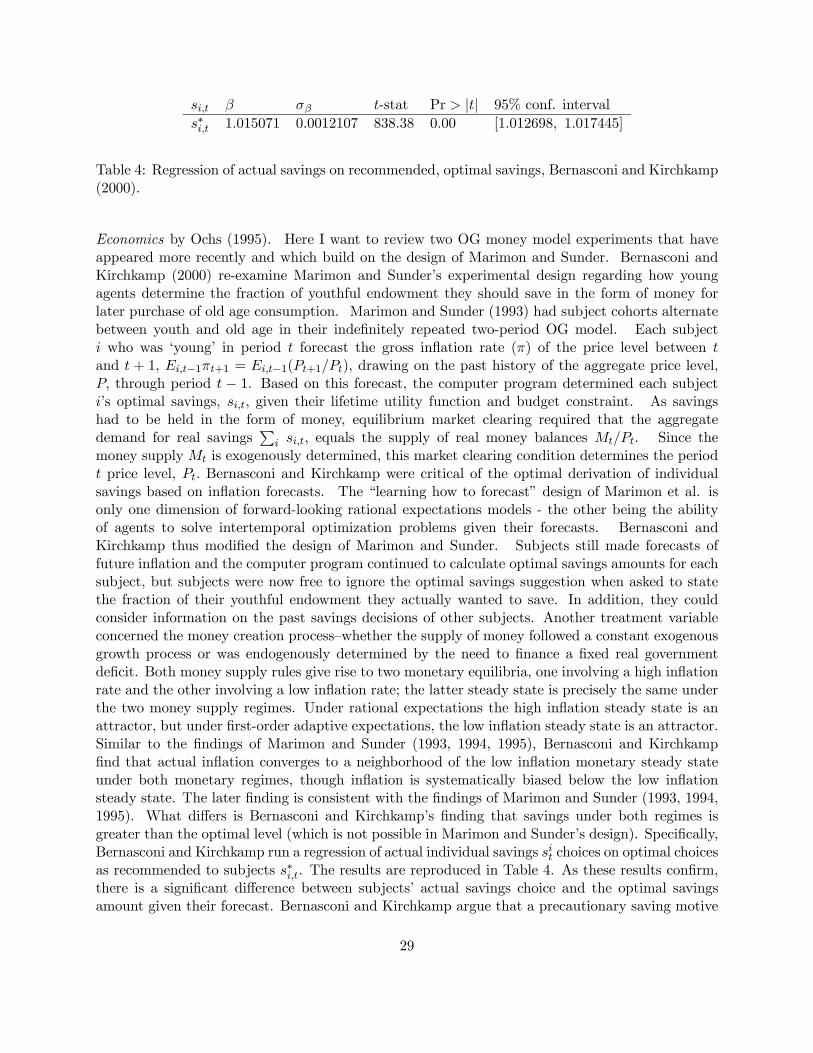
si,t β σβ t-stat Pr > |t| 95% conf. intervals∗i,t 1.015071 0.0012107 838.38 0.00 [1.012698, 1.017445]

Table 4: Regression of actual savings on recommended, optimal savings, Bernasconi and Kirchkamp(2000).

Economics by Ochs (1995). Here I want to review two OG money model experiments that haveappeared more recently and which build on the design of Marimon and Sunder. Bernasconi andKirchkamp (2000) re-examine Marimon and Sunder’s experimental design regarding how youngagents determine the fraction of youthful endowment they should save in the form of money forlater purchase of old age consumption. Marimon and Sunder (1993) had subject cohorts alternatebetween youth and old age in their indefinitely repeated two-period OG model. Each subjecti who was ‘young’ in period t forecast the gross inflation rate (π) of the price level between tand t + 1, Ei,t−1πt+1 = Ei,t−1(Pt+1/Pt), drawing on the past history of the aggregate price level,P, through period t − 1. Based on this forecast, the computer program determined each subjecti’s optimal savings, si,t, given their lifetime utility function and budget constraint. As savingshad to be held in the form of money, equilibrium market clearing required that the aggregatedemand for real savings

Pi si,t, equals the supply of real money balances Mt/Pt. Since the

money supply Mt is exogenously determined, this market clearing condition determines the periodt price level, Pt. Bernasconi and Kirchkamp were critical of the optimal derivation of individualsavings based on inflation forecasts. The “learning how to forecast” design of Marimon et al. isonly one dimension of forward-looking rational expectations models - the other being the abilityof agents to solve intertemporal optimization problems given their forecasts. Bernasconi andKirchkamp thus modified the design of Marimon and Sunder. Subjects still made forecasts offuture inflation and the computer program continued to calculate optimal savings amounts for eachsubject, but subjects were now free to ignore the optimal savings suggestion when asked to statethe fraction of their youthful endowment they actually wanted to save. In addition, they couldconsider information on the past savings decisions of other subjects. Another treatment variableconcerned the money creation process—whether the supply of money followed a constant exogenousgrowth process or was endogenously determined by the need to finance a fixed real governmentdeficit. Both money supply rules give rise to two monetary equilibria, one involving a high inflationrate and the other involving a low inflation rate; the latter steady state is precisely the same underthe two money supply regimes. Under rational expectations the high inflation steady state is anattractor, but under first-order adaptive expectations, the low inflation steady state is an attractor.Similar to the findings of Marimon and Sunder (1993, 1994, 1995), Bernasconi and Kirchkampfind that actual inflation converges to a neighborhood of the low inflation monetary steady stateunder both monetary regimes, though inflation is systematically biased below the low inflationsteady state. The later finding is consistent with the findings of Marimon and Sunder (1993, 1994,1995). What differs is Bernasconi and Kirchkamp’s finding that savings under both regimes isgreater than the optimal level (which is not possible in Marimon and Sunder’s design). Specifically,Bernasconi and Kirchkamp run a regression of actual individual savings sit choices on optimal choicesas recommended to subjects s∗i,t. The results are reproduced in Table 4. As these results confirm,there is a significant difference between subjects’ actual savings choice and the optimal savingsamount given their forecast. Bernasconi and Kirchkamp argue that a precautionary saving motive

29

arising from subjects’ uncertainty regarding their inflation forecasts can rationalize the observedover-saving behavior. This finding would appear to invalidate the use of Marimon and Sunder’s‘learning to forecast’ experimental design; subjects do not make savings decisions as if they werecertain of their forecasts of future inflation.24 Given that agents in macroeconomic models must 1)form rational expectations of future variables and 2) choose current quantities optimally in responseto those expectations, further experimental work on this important topic is required.25

Thus far, the experimental studies reviewed have considered environments where a single good,e.g., tickets, is long-lasting (durable); all other goods are perishable. If subjects perceive the durablegood to be a store of value, (perhaps owing to its durability), then that good necessarily serves asa medium of exchange, as it is the only good that can serve in that capacity. By contrast, I regardexperimental studies of the medium of exchange role of money as those which present subjectswith multiple durable goods (candidates for money) and ask whether and which of these goods isadopted by subjects as money.

Camera et al. (2003) consider the overlapping generations model with fiat money that we havejust discussed and add to it a second store of value, an interest-bearing consol.26 The questionaddressed is whether fiat money continues to be used to transfer wealth from youth to old agewhen there is an interest-bearing alternative. Understanding why money is used as a medium ofexchange when it is dominated in rate of return by other assets is a critically important issue inmonetary theory. Camera et al. explore experimentally two complementary explanations for therate of return dominance of fiat money. Their first, hoarding hypothesis — that assets bearinginterest would be hoarded and not used as media of exchange when an alternative non-interest-bearing store of value exists — is tested by initializing the economy with stocks of both fiat moneyand consols, but requiring that consols be traded pre-dividend, i.e., the dividend accrues to theowner of the consol after trading is completed. Their second, hysteresis hypothesis - that the oldhabit of using zero-interest fiat money dies hard — is tested by initializing a sequence of two-periodoverlapping generations economies with a stock of fiat money that serves as the sole store of valueand only later adding a stock of the interest-bearing consol, which trades either pre- or ex-dividendand seeing whether the fiat object continues to be used as a medium of exchange along with theconsol. money object is used as a medium of exchange. Both of these hypotheses are purelybehavioral; The stationary rational expectations equilibrium prediction in all treatments is that, inthe presence of multiple stores of value, subjects will use the good offering the highest rate of returnand a medium of exchange and eschew the other object. Consistent with the hysteresis hypothesis,the authors report that fiat money coexists with consols as a medium of exchange if there is aprior history of use of fiat objects alone as a medium of exchange. This coexistence is strongestwhen the consol dividend is paid after trade (consol is traded pre-dividend) consistent with thehoarding hypothesis. If the consol dividend is paid after trade, and consols and fiat objects areintroduced simultaneously, then subjects cease to use the fiat object and exclusively use the consolas a medium of exchange.

The use of money as a medium of exchange even though it is dominated in rate of return by

24Surprisingly, Bernasconi and Kirchkamp do not consider the same parameterization of the OG money model asexamined by Marimon and Sunder (1993, 1994, 1995), so a direct comparison is not possible.25Experiments on learning in games similarly show that subjects’ beliefs and action choices do not necessarily

coincide, and that convergence may or may not obtain as subjects acquire experience. See, e.g. Ehrblatt et al.(2007).26A consol is a bond with no terminal date paying a certain dividend per period forever.

30

other stores of value need not arise from irrational behavior. In the search theoretic approach tomoney as a medium of exchange, as pioneered by Kiyotaki and Wright (1989) and extended bymany others, equilibria can be derived in which durable goods that are not the least costly to store(have lowest return) can nevertheless serve as media of exchange under the belief that these goodswill be more readily accepted in exchange by others, thereby reducing the time it takes an individualto acquire goods he wants to consume. A second virtue of the search-theoretic approach over themodels examined previously is that exchanges of goods and money is decentralized and occurs viathe bilateral trading decisions of anonymous, randomly matched agents, which is an altogetherdifferent friction than cash-in-advance or overlapping generations. This third mechanism givingrise to the use of money seems closer to what actually occurs in monetary economies than does acentralized market clearing mechanism.

The predictions of the commodity money version of the Kiyotaki-Wright (1989) model are testedexperimentally by Brown (1996) and Duffy and Ochs (1999). In this model, there are three goods(1,2,3) and three player types (1,2,3). Player type i desires to consume good i which yields a perperiod payoff of u but type i produces good i+1 modulo 3. Hence, there is an absence of a double-coincidence of wants and some players will have to trade for goods they do not desire to consumein order to obtain goods they do desire to consume; such goods may be regarded as commoditymonies. Each player can store a single unit of a (perfectly durable) good in every period, butpays a per period storage cost ci. In the parameterization studied by Brown and Duffy and Ochs,c1 < c2 < c3. A trader starts out with a unit of his production good in storage. If he successfullytrades for his consumption good he gets the period payoff for consumption and then produces aunit of his production good, so his payoff is reduced by the cost of storing the good. Under oneparameterization of the model studied by Duffy and Ochs, all agents should play fundamental,storage-cost-minimizing strategies in equilibrium. For instance, type 2 players should trade theirproduction good 2 with type 3 players in exchange for good 1, as this lowers type 2’s storage costand reduces the time it takes type 2s to acquire their consumption good 2, via trades with type1. The predicted pattern of exchange in the unique equilibrium is as shown in Figure 7. Under adifferent parameterization, the unique equilibrium prediction -also illustrated in Figure 7— calls forsome player types to adopt speculative strategies, wherein they trade lower storage cost goods forhigher storage cost goods, e.g., type 1 players should agree to trade their production good 2 withtype 2 players for the more costly to store good 3 as this reduces the time it takes type 1 to acquireits consumption good 1. This is a case where good 3 is used as a medium of exchange by type 1even though it is dominated in rate of return (inverse of storage cost) by type 1’s production good2.

[Figure 7 here.]

Brown tested only the speculative pattern of exchange and made use of a strategy method,wherein each subject stated their trading decision for all possible player types storing all possiblegoods prior to being randomly matched with a player; trades were then executed in accordancewith strategies. Duffy and Ochs tested both sets of equilibrium trading predictions. As in Browns’study, subjects were assigned a fixed player type, but unlike in Brown’s study, following each randompairing with another player a subject had to decide whether to trade the good they had in storagefor the good of the other player; mutually agreed upon exchanges were implemented. Despite thesedifferences, the experimental findings of the two studies are quite similar as shown in Table 5, whichreports the frequencies of exchange behavior in both the speculative and fundamental environments.

31

Speculative Parameterization Type 1 trades 2 for 3 Type 2 trades 3 for 1 Type 3 trades 1 for 2Brown (1996) 0.31 0.99 0.13

Duffy & Ochs (1999) 0.36 0.93 0.25Spec. Eq. Prediction 1.00 1.00 0.00

Fundamental ParameterizationDuffy & Ochs (1999) 0.30 0.97 0.13Fund. Eq. Prediction 0.0 1.00 0.00

Table 5: Frequencies of trade offers by the three player types as reported by Brown (1996) and Duffyand Ochs (1999) in the speculative and fundamental equilibrium environments of the Kiyotaki andWright (1989) model along with equilibrium predictions

The main finding of both studies is that, inconsistent with the theoretical predictions, subjects donot adopt the play of speculative strategies when such strategies constitute the unique equilibriumprediction. In particular, only around 1/3 of type 1 subjects storing good 2 agree to trade thatgood for the more costly-to-store good 3.27 In the environment where the fundamental equilibriumis unique, Type 1s do not trade good 2 for good 3, behavior but Duffy an Ochs report that tradingdecisions by Type 1s in this environment are insignificantly different from decisions by the sametype the speculative environment (see Table 5). Duffy and Ochs argue that subjects choose tradingstrategies based on immediate past payoff experiences as opposed to the more forward-lookingmarketability considerations that the theory emphasizes.

In an effort to make marketability considerations more transparent to Type 1 players, Duffy(2001) changed the distribution of the N subjects over the three types from 1/3 of each type to 1/3of Type 1, 2/9 of Type 2 and 4/9 of Type 3. Thus, Type 1s were more likely to encounter a Type3 player and might therefore appreciate the use of the more costly-to-store good 3 as a medium ofexchange. Indeed, Duffy (2001) reports an increase in the acceptance of good 3 by Type 1 playersfrom the 36% rate reported in Duffy and Ochs for the equal distribution of player across typesto an acceptance frequency of 67% under the asymmetric distribution (still below the speculativefrequency of 100%). Automating the decisions of Type 2 and 3 players with robot traders whoplayed fundamental trading strategies also helped to boost speculative trades by Type 1 players toan average of 73%. These findings suggest that there exist certain parameterizations of the modelin which a majority of subjects can learn to adopt speculative strategies where the money good isdominated in rate of return by other potential stores of value.

All of the goods in the search experiments described above had consumption value to one typeof player. Duffy and Ochs (2002) add to this same environment an exogenous supply of a fourthgood, 0 which is neither produced nor consumed by any player type. The question they pose iswhether an intrinsically worthless fiat object that is not invested with value by legal restriction,would come to be used as a medium of exchange. Kiyotaki and Wright (1989) show that equilibriawhere this object is or is not traded coexist, so the issue is one of equilibrium selection. Duffy andOchs’ (2002) experimental finding is that an intrinsically worthless fiat object will circulate as amedium of exchange so long as it has the lowest storage cost; if it is not the least-costly to store

27 Interestingly, this same lack of speculation finding is also obtained in agent-based model simulation conductedby Marimon et al. (1990), which was the inspiration for both the Brown and Duffy and Ochs studies.

32

good, i.e., if it is dominated in rate-of-return, then its circulation as a medium of exchange is morelimited than predicted by the theory.

Money’s role as a unit of account is uncontroversial; prices are typically quoted in terms ofmoney units and not in terms of (say) artichokes. However, as money typically depreciates invalue over time due to inflation, most macroeconomic models presume that agents evaluate allchoice variables in real terms, taking into account changes in the purchasing power of money.Experimental studies of money as a unit of account assess the extent to which individuals evaluatemagnitudes in real terms or, alternatively are subject to money illusion - the failure to adjustnominal values for changing prices. Motivated by survey evidence of money illusion (Shafir et al.1997) and on the downward stickiness of nominal prices and wages (Bewley 1999), Fehr and Tyran(2001, 2007, 2008) have conducted several experimental studies documenting money illusion and itsconsequences for nominal inertia. In the first of these studies, Fehr and Tyran have subjects playan n-player “price—setting” game. In each of 2T periods, subject i chooses a price Pi and earns areal payoff that is a function of the time t average price chosen by other players, P−i,t and the timet nominal money supply Mt:

πi,t = f(Pi, P−i,t,Mt)

The function f yields a unique, dominance-solvable equilibrium for every value of M , is homoge-neous of degree 0 in all arguments, and fP−i,t ≥ 0, so there is a weak strategic complementarityin price-setting. In addition to treatments where subjects are paid according to this real payofffunction, there is also a nominal payoff treatment where subjects’ earnings are reported to them innominal terms, P−1πi. Subjects are instructed on how they can deflate these payoffs into real termsby dividing by P−1. Fehr and Tyran characterize money illusion as a framing effect ; behavior ispredicted to differ depending on whether subjects are paid in real price adjusted terms, or in nom-inal terms. The difference comes in the adjustment to a nominal shock: the nominal money supplyis known to be a constant level M for the first T periods and then to decline to a permanentlylower level λM , λ < 1 for the last T periods. The issue addressed is whether subjects will adjusttheir prices downward at date T from P to λP , an adjustment that is more difficult in the nominalpayoff function treatment where subjects have to correctly deflate their nominal payoff function.A second difficulty, arising from the strategic complementarity in price setting, is that the failureof some subjects to adjust to the nominal shock may make it a best response for others who arenot subject to money illusion to only partially adjust to the shock themselves. To eliminate thelatter possibility, Fehr and Tyran conduct individual-decision making experiments under both thereal and nominal payoff functions where the other n− 1 players are known to the human subjectsto be robot players who are not subject to money illusion and who will adjust prices downwardproportional to the shock and at the time of the shock.

[Figure 8 here.]

The experimental findings are nicely summarized in Figure 8, where we see that in three ofthe four treatments, the downward adjustment of prices to the new equilibrium occurs almost im-mediately following the fully anticipated reduction in M , whereas in the nominal payoff functionwith human opponents treatment, price adjustment is considerably more sluggish. Fehr and Tyranattribute behavior in the latter treatment to “the belief that there are subjects who take nominalpayoffs as a proxy for real payoffs,” which leads those who hold those beliefs to adjust their pricesmore slowly. When the payoff function is presented in real terms or there are computerized oppo-nents, such beliefs are unwarranted, and so the extent of price sluggishness is greatly diminished, if

33

not perfectly eliminated. Fehr and Tyran further show that prices adjust more rapidly in responseto a positive shock than they do in response to a negative shock.

Fehr and Tryan (2007) consider a modified version of their price-setting game in which thereare three Pareto-ranked equilibria. In real terms, the ranking of payoffs was πA > πC > πB, butin nominal terms, the ranking was: PCπC > PAπA > PBπB. The treatments were as in theirearlier study: whether payoffs were presented in real or nominal terms and whether subjects playedagainst n − 1 human or computer opponents. As before subjects are instructed in how to deflatenominal payoffs into real terms. Unlike the prior experiment, the focus here is not on adjustment toa shock but rather on equilibrium selection. In the computerized treatments, the n− 1 robots playa best response to the past history of play of the human subject, effectively making the subject aStackelberg leader. Fehr and Tyran’s main finding is that in the nominal treatment with humanopponents, subjects coordinate on the inefficient C equilibrium while in the real treatment withhuman opponents they coordinate on the efficient A equilibrium; they interpret this as evidence ofmoney illusion. In the nominal or real treatments with computerized opponents, with experiencesubjects get close to the efficient equilibrium, though not as close as in the real payoff treatmentwith human opponents; they attribute the latter to imitation of the choices of other human actors,as reflected in prices observed each period.

In a third study, Fehr and Tyran (2008) consider not only the prior case where there is astrategic complementarity in price setting, but now also consider the case where there is strategicsubstitutability in price setting, i.e. fP−i,t ≤ 0. They report that money illusion and the resultingnominal inertia in response to a fully anticipated monetary shock is greatly reduced in the case ofstrategic substitutes relative to the case of strategic complements. In the substitutes case, errorsunder adaptive learning are much greater following the money shock leading to much faster adjust-ment toward more rational behavior than in the complements case. Thus, it appears important toconsider the strategic environment in assessing the extent to which money illusion may matter fornominal inertia.

Summing up, laboratory monetary experiments have examined whether individuals thinks inreal or nominal terms, and have explored the circumstances under which a token object can serveas a store of value as well as the characteristics of stores of value that make them more readilyacceptable as media of exchange. While the experimental literature on monetary questions is oneof the largest in experimental macroeconomics, there remains much further work to be done. Forinstance, most of the experimental studies of money we have discussed have fixed rates of exchangebetween money and goods ignoring the important role of prices. Allowing for prices, one couldthen begin to think about exchange rate determination between multiple money objects.28 Whilemoney illusion (together with the strategic environment) is an interesting explanation for nominalprice stickiness, it is by no means the only explanation and indeed, most macroeconomists wouldpoint to other sources, including informational frictions, costly price or information adjustment orstaggered contracting. Experimental studies of the behavioral relevance of these other mechanismsis an important an open question for future research.

4.2 Labor Economics

Empirical research in labor economics typically involves the use of large panel data sets as assem-bled by government agencies. However there is also a small and growing experimental literature

28For one early attempt, see the discussion of Arifovic (1996) below.

34

that exploits the greater control and identification of causal relationships that is afforded by thelaboratory relative to the field (see, e.g., Falk and Gächter (2008) and Falk and Fehr (2003)). HereI focus on some of the labor economic experiments that should be of interest to macroeconomists.

An early experimental literature (previously reviewed by Camerer (1995)) examined individualbehavior in intertemporal one-sided job search models that are commonly used to study unem-ployment and labor-market policies (e.g. as surveyed by Mortensen (1987)). Experimental studiestesting many of the comparative static implications of job search models include Braunstein andSchotter (1981, 1982), Hey (1987), Cox and Oaxaca (1989, 1992), Harrison and Morgan (1990)).For instance, Braunstein and Schotter (1981) test a number of theoretical hypotheses involvingthe one-sided model of intertemporal optimal job search with or without perfect recall. In thismodel, an unemployed worker draws a wage offer each period and must decide whether to acceptor reject each offer taking into account the known probability distribution of wage offers, searchcosts and the level of unemployment compensation (if any). The optimal search strategy involvescalculation of a reservation wage level; wage offers at or above this level are accepted and thosebelow it are rejected. Braunstein and Schotter (1981) report experimental evidence in support ofthe notion that individuals choose reservation wages that are nearly optimal and accept or rejectoffers relative to this wage level. Among the treatment variables they consider are different wagedistribution functions, search costs and whether subjects could recall past wage offers or faceduncertainty about the wage distribution function they faced.

In addition to intertemporal labor force participation decisions, another labor market choiceof interest to macroeconomists that has received some experimental attention, is the labor-leisuretrade-off. An increase in wages may have both substitution and income effects on hours worked.The impact of wage changes on labor supply is an important empirical question, as most businesscycle models require the (compensated) elasticity of labor supply to be positive and sufficientlylarge so that transitory shocks can generate the large volatility in hours worked that is observed inmacroeconomic data.29 Battalio, Green and Kagel (1981) report experimental evidence confirmingpositive compensated wage effects on time spent working, though their experiments involved pigeonsrather than human subjects. In particular, Battalio et al. report that nearly all of their hungryPigeons responded to a Slutsky-compensated wage decrease with a reduction in labor supply, whichinvolved pecking a key.

Using human subjects, Dickinson (1999) has experimentally examined two extensions to theclassical labor supply model. In the first, hours of work are no longer a choice variable, but areinstead fixed - a situation that characterizes many (short-run) employment relationships; indeedsome business cycle theorists have exploited this type of nonconvexity as a means of increasingvolatility in hours worked. However, in contrast to the standard theory, which assumes that workersprovide full effort when on the job, Dickinson allows subjects to choose the intensity of their workeffort; essentially they can decide whether to take on-the-job leisure. Specifically, subjects mustparticipate in a two hour experiment during which time they are asked to type an unlimitedsupply of paragraphs, earning a fixed wage for every paragraph they type with no more than afew errors. The intensity of their work effort is examined in response to compensated changes inthe (piece-rate) wage. Compensation was achieved by varying the value of non-labor income. Thiskind of data on labor effort is typically unavailable to labor economists (who at most can observelabor hours) and serves to illustrate one of the advantages of study labor market theories in the

29Most estimates based on microeconomic data find the compensated elasticity to be small or even negative.

35

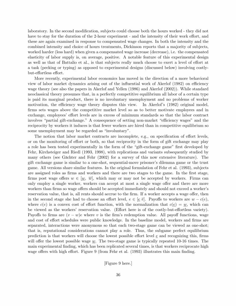
laboratory. In the second modification, subjects could choose both the hours worked - they did nothave to stay for the duration of the 2-hour experiment - and the intensity of their work effort, andthese are again examined in response to compensated wage changes. In both the intensity and thecombined intensity and choice of hours treatments, Dickinson reports that a majority of subjects,worked harder (less hard) when given a compensated wage increase (decrease), i.e. the compensatedelasticity of labor supply is, on average, positive. A notable feature of this experimental designas well as that of Battalio et al., is that subjects really much choose to exert a level of effort ata task (pecking or typing) as opposed to experimental designs (discussed below) involving costly-but-effortless effort.

More recently, experimental labor economics has moved in the direction of a more behavioralview of labor market dynamics arising out of the influential work of Akerlof (1982) on efficiencywage theory (see also the papers in Akerlof and Yellen (1986) and Akerlof (2002)). While standardneoclassical theory presumes that, in a perfectly competitive equilibrium all labor of a certain typeis paid its marginal product, there is no involuntary unemployment and no problems of workermotivation, the efficiency wage theory disputes this view. In Akerlof’s (1982) original model,firms sets wages above the competitive market level so as to better motivate employees and inexchange, employees’ effort levels are in excess of minimum standards so that the labor contractinvolves “partial gift-exchange.” A consequence of setting non-market “efficiency wages” and thereciprocity by workers it induces is that fewer workers are hired than in competitive equilibrium sosome unemployment may be regarded as “involuntary”.

The notion that labor market contracts are incomplete, e.g., on specification of effort levels,or on the monitoring of effort or both, so that reciprocity in the form of gift exchange may playa role has been tested experimentally in the form of the “gift-exchange game” first developed byFehr, Kirchsteiger and Riedl (1993, 1998), with replications and variants subsequently studied bymany others (see Gächter and Fehr (2002) for a survey of this now extensive literature). Thegift exchange game is similar to a one-shot, sequential-move prisoner’s dilemma game or the trustgame. All versions share similar features. In the original formulation of Fehr et al. (1993), subjectsare assigned roles as firms and workers and there are two stages to the game. In the first stage,firms post wage offers w ∈ [w, w], which may or may not be accepted by workers. Firms canonly employ a single worker, workers can accept at most a single wage offer and there are moreworkers than firms so wage offers should be accepted immediately and should not exceed a worker’sreservation value, that is, all rents should accrue to the firm. If a worker accepts a wage offer, thenin the second stage she had to choose an effort level, e ∈ [e e]. Payoffs to workers are w − c(e),where c(e) is a convex cost of effort function, with the normalization that c(e) = w, which canbe viewed as the workers’ reservation value. (Effort here is of the costly-but-effortless variety).Payoffs to firms are (v − w)e where v is the firm’s redemption value. All payoff functions, wageand cost of effort schedules were public knowledge. In the baseline model, workers and firms areseparated, interactions were anonymous so that each two-stage game can be viewed as one-shot;that is, reputational considerations cannot play a role. Thus, the subgame perfect equilibriumprediction is that workers will choose the lowest possible effort level e and recognizing this, firmswill offer the lowest possible wage w. The two-stage game is typically repeated 10-16 times. Themain experimental finding, which has been replicated several times, is that workers reciprocate highwage offers with high effort. Figure 9 (from Fehr et al. (1993) illustrates this main finding.

[Figure 9 here.]

36

In this Figure, the competitive equilibrium (and lowest possible) wage w = 30 which is associatedwith minimum effort level e = 0.1. The maximum possible wage is 110 and the maximum effortlevel was 1. A wage of 30 was observed only once, and workers chose the minimum effort level only16% of the time. The average wage was 72 and the average effort level was .4, both well above thecompetitive equilibrium predictions.

Fehr and Falk (1999) modify the first stage of the gift-exchange game so that both firms andworkers can propose and accept wage offers via a double auction, following the standard improve-ment rules. In the second stage, worker effort was either exogenously fixed by the experimenter, sothat the contract negotiated in the first stage was “complete,” or workers were free to choose effortlevels in the second stage, the case of “incomplete” wage contracts. As in the prior experiments,there were more workers than firms, so one would expect workers to underbid one another downto their minimum, reservation wage levels. Fehr and Falk report two main findings. First, whencontracts are completely specified by a wage offer (effort predetermined) this wage tends to beclose to the competitive equilibrium level, where all rents accrue to the firm due to the smallernumber of firms relative to workers. Second, when workers are free to choose effort levels, wagesare significantly above competitive equilibrium levels as in the earlier experiments where only firmscould make wage offers. These higher wages are not because workers are refusing to undercutone another (a possibility suggested by Solow (1990)); Falk and Fehr report that there is, in fact,“massive underbidding” by workers seeking to secure wage offers. Interestingly most firms refuseto accept these low wage offers; while bid improvement rules force workers’ wage offers to fall, firmsare free to accept any wage offer and choose only to contract at wages well above workers’ reserva-tion levels. Subjects in the role of firms recognize that subjects in the role of workers will providegreater effort the greater is the wage offered, and this recognition results in sticky downward wagerigidity. This evidence is consistent with survey evidence, e.g. by Bewley (1999) indicating thatmanagers recognize the impact of low wages on employee morale.

In a third set of experiments, Fehr et al. (1996, 1997) and Fehr and Gächter (2002) furthermodify the basic experimental design of Fehr et al. (1993) so that in the first stage, the wage contractspecifies a wage, a desired effort level and a fine for effort below the desired level. A third stage isadded in which the worker’s effort level is probabilistically monitored by the experimenter; if belowthe desired level, the worker pays an fixed and publicly known fine to the firm. This design can beviewed as a version of Shapiro and Stiglitz’s (1984) deterrence—of—shirking version of the efficiencywage model though in that model, a worker detected to be shirking is fired rather than fined. Theissue explored in these experiments is whether the specification of desired effort levels, monitoringand fines i.e., incentive contracting, undermines the positive reciprocity observed in experimentswhere these feature of the wage contract are unspecified. The results are somewhat mixed. On theone hand, firms are able to obtain effort levels above the requested level by setting high, “efficiencywages” as in the earlier experiments. On the other hand, firms tended to request too much effortand set wages too low to enforce a no-shirking outcome given the fines workers faced. Consequently,there is a substantial amount of shirking, despite the no-shirking-in-equilibrium prediction of theShapiro-Stiglitz model.

Summarizing, experimental research pertaining to the labor market finds some support for thecomparative static implications of rational job search models and labor-leisure decisions. Whilethat work focuses exclusively on labor supply decisions, work by Fehr and associates has consid-ered both labor demand and supply decisions. Consistent with efficiency wage theories, Fehr andassociates have provided evidence that incomplete labor contracts and reciprocity concerns can

37

lead to above market clearing wages and involuntary unemployment. The collection of papers byFehr and associates in particular is an excellent illustration of how a body of knowledge can bebuilt up from a simple experimental game, to which additional features are incrementally added.The evidence provided in all of these studies, e.g. on the formation of reservation wages or theextent of involuntary unemployment would be difficult to observe or identify outside the controlledenvironment of the laboratory.

4.3 International Economics

A third sector of the macro-economy where experimental methods have been employed is theinternational sector. The justifications for an experimental approach to international economicsare similar to those we have seen before: the available field data does not allow for precise tests oftheoretical predictions nor is it possible to abstract away from complicating factors, for example,transport costs or multi-lateral as opposed to bilateral two-country trade (most theoretical modelsassume the latter).

Noussair et al. (1995) conducted the first experimental test of two key principles of internationaltrade: comparative advantage and factor price equalization. They consider two experimental envi-ronments involving 8-16 subjects each. The first is a labor-only, Ricardian model and the second isone where both capital and labor are used as inputs into production.30 In both environments thereare two countries and within each country two player types: consumers and producers. Producersand consumers have induced desires to produce and consume quantities of the two goods Y and Z.In the Ricardian model, consumers inelastically supply labor L to producers for “francs” (money)which they use to buy quantities of the producers’ goods Y and Z. Producers use labor as inputinto production of good Y and Z. There are equal numbers of consumers and producers in eachcountry and all subjects have the same endowments of labor and money. The two countries differonly in their production technologies:

Country 1 Y1 = 3L1 Z1 = L1Country 2 Y2 = L1, Z2 = 2L2

Thus country 1 (2) has a comparative advantage in the production of good Y (Z). While laborsupplies, L1 and L2, are not mobile across countries, trade in goods is possible, and there is noperceived difference in good Y (Z) produced by either country. Thus in the Ricardian model, thereare six markets, two internal labor markets and four external goods markets for the two goodsY, Z, produced by each of the two countries. These were implemented using computerized doubleauctions and induced values for inputs (by producers) and for goods bought (by consumers) andsold (by producers). The main hypothesis tested in this design is the law of comparative advantage;in the competitive equilibrium, trade occurs in the sense that members of two countries buy and sellgoods Y and Z to one another with county 1 completely specialized in the production (sales) of goodY and country 2 completely specialized in the production (sales) of good Z. This prediction maybe contrasted with the inefficient autarkic outcome in which there is no trade between countries,and hence no specialization. The second environment which adds capital, differed in that the twocountries had identical linear production technologies, i.e., Y = L and Z = K in both countries,but different aggregate endowments of labor and capital and there was now an internal market forboth labor and capital (both immobile factors). Thus this economy had eight markets. The main

30The first experiment involving both input and output markets was conducted by Goodfellow and Plott (1990).

38

prediction of this environment is that both countries produced both goods and in the competitiveequilibrium, country 1 would be a net exporter of good Y and country 2 a net exporter of good Z.Further, in the competitive equilibrium, prices of the two goods should be equalized across countriesand this further implies factor price equalization. Such equalization does not occur under autarky.

The experimental results are somewhat mixed. On the one hand, there is strong support for thelaw of comparative advantage; in the Ricardian environment there is nearly complete specializa-tion by producers in the two countries, and in the environment with capital, the two countries netexports are of the good for which they hold a comparative advantage. Further in the environmentwith capital, output prices are equalized across countries and given the identical linear productionfunctions, so are factor prices. The latter finding is one that would be very difficult to observeoutside of the controlled environment of the laboratory, as it only holds in special cases such as theone induced here. On the other hand, input and output prices are neither consistent with compet-itive equilibrium or with autarkic levels. Noussair et al. argue that production and consumptionpatterns appear to be converging toward competitive equilibrium levels especially under free trade(they also consider some environments with tariffs). As evidence for convergence, they make useof regression equations of the type (1) discussed earlier in section 2.1.

In a related paper, Noussair et al. (1997) focus on issues of international finance: exchangerate determination, the law of one price and purchasing power parity. They simplify the set-upfrom their prior experiment so that there is no longer any factor inputs or production processes;there is simply an endowment of two final goods X and Y in each of the two countries, A and B.A further difference is that each country now has its own money. Each country was populatedby six subjects, three of whom were sellers of (endowed with) good X and buyers of good Y andthe other three were sellers of (endowed with) good Y and buyers of good X. In addition subjectswere endowed with amounts of their home currency only. As in the prior study, a demander ofgood X was indifferent between acquiring X from a supplier in his home country or in the foreigncountry. However, foreign country purchases required acquisition (cash) in advance of the foreigncurrency. A further restriction designed to force the use of currency markets was that residents ofone country could not transport and sell goods abroad so as to obtain foreign currency for purchasesabroad. (On the other hand, goods purchased abroad could be costlessly transported home). Ineach country, markets in the two goods and foreign currency were implemented using computerizeddouble auctions. Subjects were induced to value quantities of goods X or Y and the home currencyonly; the end-of-session redemption value of any foreign currency holdings was zero.

The exchange rate e —the price of currency A in terms of currency B — is determined accordingto the balance of payments approach wherein e equates the demand and supply for currencies Aand B arising out of the flow of international transactions, as predicted by comparative advantage:in the competitive equilibrium, country A (B) is an importer of good X (Y). Given this balance ofpayments view, and supposing that trade occurs, the main hypothesis tested concerns the law ofone price:

ePAX = PB

X ePAY = PB

Y

or that adjusting for exchange rates, goods X and Y have a single world price. The alternativehypothesis is again, that the inefficient, autarkic, no-trade outcome is realized in which case thelaw of one price does not hold.

The experimental findings are somewhat mixed, though the authors conclude that their dataare closer to the competitive equilibrium than to the autarkic predictions, again using regressionequations of the type (1). On the one hand, they find somewhat remarkable (given the complexity of

39

the environment) evidence of convergences to the competitive equilibrium exchange rate predictione = 47 across four sessions as shown in Figure 10. On the other hand, the law of one price (and avariant, purchasing power parity, that is based on price level indices) fails to obtain. Noussair etal. (1997) conjecture that this failure arises because of different speeds of convergence of prices inthe two domestic markets, which leads to a failure of the law of one price even though the exchangerate is at the competitive equilibrium level. Increasing the duration of the experiment beyond theten 15-minute trading periods in a session might have allowed for such a convergence to take place.

[Figure 10 here.]

One observation regarding this pair of experiments is that the autarkic outcome, while soundlyrejected, is something of a straw man; absent restrictions on trade, the no-trade outcome does notcomprise an equilibrium and is rationalized as being plausible if subjects are so averse to foreignexchange market uncertainty that they refuse to engage in trade. Nevertheless, the important valueof these experiments in illustrating how basic tenets of international trade and finance can be testedin the laboratory cannot be emphasized enough, and much further work could be done along thesesame, lines e.g., allow capital flows across countries.

Some theoretical work on exchange rate determination is in environments where there are norestrictions on portfolio holdings and the demands for currencies are endogenously derived, as op-posed to the cash-in-advance induced demand for currency in the design of Noussair et al. 1997.In this more general environment, if two monies are perfect substitutes and there is no govern-ment intervention in currency markets or legal restrictions on currency holdings, the exchange ratemay be indeterminate. Further, if agents have perfect foresight it is predicted that whatever theexchange rate turns out to be, it will be invariant over time, as in the overlapping generationsmodel of Kareken and Wallace (1981). These two predictions are tested in an experiment by Ar-ifovic (1996) that was designed for comparison with the predictions of an agent-based model (agenetic algorithm). In the experiment there was a single consumption good and equal, fixed sup-plies of two currencies, francs and lire. As the environment is an overlapping generations model,even/odd-numbered subjects alternated every even/odd period between being young and receivingendowment ωy of the consumption good and being old and receiving endowment ωo of the consump-tion good with ωy > ωo. They were then reborn as young agents, repeating the two-period cycleof life anew. Subjects were induced to hold log preferences over consumption in the two periodsof life, so their optimal plan involves consumption smoothing, or selling some of their endowmentfor the two monies (the only stores of value) when young and redeeming these money holdings inthe next period at prevailing prices for old-age consumption. Initial period “old” subjects wereendowed with equal amounts of the 10 units of the two currencies. Each young subject was calledon to make two decisions - how much of their youthful endowment to save (the remainder wasconsumed) and what fraction of their savings was to be held in domestic currency; the remainderwas placed in foreign currency holdings. Old subjects inelastically supplied their money holdingsfor consumption. The exchange rate between the two currencies was that which equated youthfuldemands for, and old agent supplies of the two currencies. The main experimental finding (fromjust two experimental sessions!) was that the mean exchange rate was about 1, but counter tothe stationary perfect foresight equilibrium prediction, there was persistent fluctuations in the ex-change rate. Arifovic attributes this volatility to small changes in the portfolio decisions of youngagents in response to immediate past differences in rates of return on the two currencies, whichin turn generates volatility in the exchange rate in a continual feedback loop. Observed volatility

40

in exchanges rates has been difficult to explain - many attribute it to “news” or “sunspots” — butArifovic’s experimental finding of adaptive learning dynamics with regard to portfolio decisionsprovides a new alternative.

Fisher (2001) revisits the issue of the law of one price and purchasing power parity that Noussairand associates failed to observe in their experiment by constructing a greatly simplified, version ofthe Noussair et al. (1997) environment. In Fisher’s design, each country produces only a singlegood, the prices and supplies of which are perfectly controlled by the experimenter, so the mainjob of subjects (as in Arifovic (1996)), is to determine the nominal exchange rate. The two goodsand currencies are “green” (domestic) and “red” (foreign), and green(red) currency is required inadvance to buy green (red) goods (so, this is again the case of a cash-in-advance induced demand forcurrency). Each subject begins a session endowed only with a large supply of the green currency.31

The price and end-of-session redemption value of a unit of the green good, pg and vg are fixedand known for the duration of a session as is the end-of session redemption value of a unit of thered good, vr and the green currency. Red currency is in limited supply, has no end-of sessionredemption value and cannot be carried over from one period to the next; its main purpose isto purchase the red good. The red currency price of a unit of the red good in period t, prt , —atreatment variable— is randomly determined from a set of values and announced at the beginningof each of the 10 periods that comprise a session. Supplies of the two goods are unlimited, butvr > vg, which motivates a demand for the red good and red currency. The limited supply of redcurrency each period, equal to just k − 2 units where k is the number of subjects, is held by theexperimenter. After the unit price of the red good for the period (prt ) is announced, the supply ofred currency is auctioned off in a second-price, sealed bid auction. Each subject could bid amountsof green currency for just one of k − 2 units of red currency during this first auction phase of aperiod. The market-clearing price of a unit of red (foreign) currency in terms of green (domestic)currency (equal to the second lowest bid submitted) is interpreted as the nominal exchange ratefor period t, et. Once et is determined, subjects were free to buy units of green and red goodssubject to cash-in-advance and budget constraints. Fisher’s main hypothesis - a relative version ofpurchasing power parity -is that the real exchange rate in each period t, defined by qt = etp

rt/p

g, isinvariant over time, i.e., that the market clearing, nominal exchange rate et immediately adjusts tothe announced red good prices, prt so as to keep the real rate, qt, constant. A related hypothesis,absolute purchasing power parity, posits that the real exchange rate qt equals vr/vg, the marginalrate of substitution between foreign and domestic goods, so the nominal exchange rate in eachperiod is determined according to:

et =vrpg

vgprt.

Thus Fisher’s exchange rate determination process arises out of purchasing power parity as opposedto the balance of payments approach to exchange rate determination followed by Noussair et al.which relies on trade flows between countries. With this stripped down experimental design involv-ing perfectly controlled prices, Fisher finds convincing evidence for both the relative and absoluteversions of purchasing power parity. This finding confirms a conjecture of Noussair et al. thatthe failure of purchasing power parity in their study was likely owing to the slow and differentialconvergence of prices in the goods markets; in Fisher’s design there is no problem with non conver-gence of goods prices as these are pre-determined. Fisher also adds an interest rate to red currency31As in Arifovic (1996), one can think of all the subjects in Fisher (2001) as residing in the domestic country only,

but having access to foreign currency.

41

holdings over a subperiod of each period as well as uncertainty regarding the price of the red goodin order to test hypotheses related to covered and uncovered interest parity. He finds support forthese hypotheses as well.

Having studied a greatly simplified exchange rate environment, Fisher (2005), in a follow-uppaper, seeks to understand two complicating factors that might account for the widespread lackof evidence in support of purchasing power parity and (un)covered interest parity in econometricanalyses of historical field data.32 He considers the role of 1) non-traded goods, which if sizeable,may lead to failures of purchasing power parity in analyses using aggregate price indices, and 2)non-stationary price level dynamics. Proxies for these two complicating factors are introduced intothe design of Fisher (2001). Both non-traded goods and non-stationary goods prices are found toincrease the deviation of exchange rates from theoretical predictions, with the largest deviationscoming from the environment with non-stationary prices.

Summarizing, the laboratory has been used to test some basic principles of international eco-nomics including the law of comparative advantage, the law of one price and theories of exchangerate determination and the notion of purchasing power parity. These are phenomena that are ei-ther difficult to test (comparative advantage) explain (exchange rate volatility) or which have beenrefuted in econometric tests with available field data (purchasing power parity). We have seenhow experimental methods can shed light on these topics and how building on prior experimentaldesigns can help to clarify puzzling findings, such as Noussair et al.’s finding that purchasing powerparity does not hold. Further work on this topic might consider adding dynamic, intertemporallinkages such as would occur by adding capital accumulation or considering intertemporal con-sumption savings/decisions. One shortcoming of the international experiments reported on here isthat, with the exception of Fisher (2005), the number of experimental sessions of a treatment aretoo few. In implementing complex international economic environments, the temptation is to loadup each session with many changes in treatment variables, a practice that is understandable, butone that should be avoided nonetheless.

4.4 Multi-sectoral Macroeconomics

A few courageous researchers (namely Charles Plott and associates), have sought to combine allthree of the sectors we have explored in the last few sections by implementing large-scale laboratorymacroeconomies. Such multi-sectoral systems involving simultaneous markets for factor inputs,goods, money as well as foreign goods and money, may be what many people have in mind whenthey hear the term “macroeconomic experiments.” I hope it is clear by now that a macroeconomicexperiment need not be elephantine; rather it suffices that the experiment addresses a topic ofinterest to macroeconomists. Nevertheless, it is of interest to understand the extent to whichmany interlinked experimental markets can operate simultaneously, so as to identify the source ofinefficiencies.

A first effort at developing such a multi-sectoral laboratory macroeconomy is found in Lian andPlott (1998) who implement a static, Walrasian competitive general equilibrium model. There aretwo types of agents, consumers and producers, two goods, X and Y and a constant supply of fiatmoney. Consumers were induced to have a preference function U(X,Y ) over the two goods. Eachperiod they were endowed with 0 units of X and a constant amount of Y ; X can be interpreted as

32For instance, random walk models have consistently outperformed any economic theory of exchange rate dynam-ics.

42

a consumption good and Y as labor/leisure. Producers desired good Y only, and could consumeit directly (e.g., labor services) or use it as input into production. Producers were endowed with aconcave, labor only production technology yielding f(Y ) amount of good X for Y units of input.Producers were endowed with an amount of fiat money and good X in the first period only; theseendowments were not refreshed in subsequent periods (e.g. a constant money supply). In simulta-neously operating, multi-unit double auctions, consumers could trade good Y with producers forfiat money and consumers could purchase good X from producers in exchange for fiat money - i.e.a cash-in-advance constraint was binding. Units of X or Y that were consumed/used as input intoproduction left the system (subjects received redemption values for these based on their inducedutility/production functions). Somewhat strangely, remaining balances of X and Y were carriedforward to the next period, investing consumption and labor with a durability -and asset value—that they would not ordinarily possess (and which would have obviated the need for fiat money,absent cash-in-advance constraints). Finally, all subjects (producers and consumers) had access toa financial market where they could borrow and lend to one another in fiat-money-denominatedcontracts through a one-period bond market. Default was discouraged through the use of largeexogenous fines. Given the initial cash endowments, in the static competitive equilibrium resultingfrom consumer and producer optimization, there are no cash constraints and financial marketsshould not operate. However, there is a unique equilibrium volume of production and consumptionof goods and ratio of the price of a unit of Y to a unit of X that is independent of the numberof subjects. Each session consisted of a number of periods. The final period was not announcedin advance; market prices during that final period were used to evaluate final inventory holdingswhich were redeemed into cash at a fixed rate.

The economy is illustrated in Figure 11, which also gives the induced utility and productionfunctions used in the study.

[Insert Figure 11 here.]

Subjects for this study were nontraditional, consisting primarily of high school students par-ticipating in a summer school program at CalTech. In addition, one session involved science andengineering graduate students from the People’s Republic of China. Aside from these differentsubject populations, the main treatment variables were variations in the exogenous money supplyand the experience level of subjects (whether they participated in more than one session).

Among the main findings, Lian and Plott provide convincing evidence that there is considerableorder to the observed economic activity. Using regression equations of the form (1), they show thatconvergence toward the competitive equilibrium outcome appears to be occurring, albeit slowly;indeed, they formally reject the hypothesis that the competitive equilibrium is actually achieved.Still, the ratio of the price of Y to the price of X, predicted to be 2, is found to be around this level inall sessions. Volume in both the input and output markets is only slightly less than predicted, andthis is attributed to overconsumption of Y by consumers and underproduction of X by producers,who also overconsumed Y . Financial markets are rarely used as predicted. Experience is shown tomatter greatly in reducing the volatility of prices and volume and improving efficiency. Changes inthe money supply have proportionate effects on the price level but no real effects, and the velocity ofcirculation of money appears to hit a constant level, especially with experience. Perhaps the mostintriguing findings are based on constructed measures of unemployment, inflation and real GNP.Using these, Lian and Plott 1) find no evidence for any inflation-output Phillips-curve type trade-off and 2) strong support for a negative trade-off between changes in the unemployment rate and

43

changes in real GDP (a version of Okun’s law33 With a keen knowledge of how their macroeconomyoperates, Lian and Plott interpret the latter phenomenon as “no surprise...A fall in unemploymenttranslates to an increase in system efficiency and that becomes an increase in income and thus realGNP. (p. 62).”

Building on Lian and Plott (1998) as well as Noussair et al. (1995, 1997), Noussair et al.(2007) develop an experimental multi-sectoral macroeconomy which they claim [p. 50] is “far morecomplex than any laboratory economies created to date.” This claim cannot be disputed. Theeconomy has 3 output goods, x, y, and z, two factor inputs, labor l and capital k all of whichare specific to one of three countries A, B and C, each of which has their own currency, a b c.Thus there are 21 double auction markets in simultaneous operation — 7 markets in each country- the three goods markets, the two input markets and two currency markets. Three experimentalsessions were conducted each involving in excess of 50 subjects; two of the three experiments wereconducted remotely via the internet. The subjects were divided up roughly equally into twelvetypes, with each type being characterized by a country of residence and typically assigned two ofthree possible roles: as a producer of output goods, consumer of two output goods or supplier ofinput goods. The precise roles of each subject type, their (continuous) induced production functionf(k, l), utility function over the two goods U(·, ·) and/or supply of input cost function C(k, l) isgiven in Table 4.4

The actual functions were discretized and presented to subjects as tables. Using the inducedfunctions in Table 4.4, aggregate demand and supply functions can be calculated. Using these,the competitive equilibrium can be found using 15 market clearing conditions for output and inputmarkets, together with three law-of-one price (no arbitrage conditions) and three flow of fundsequations determining exchange rates (country A,B,C has a comparative and absolute advantagein x, y, z, respectively. As in Noussair et al. (1997), the main comparison is between the efficient,full trade, competitive equilibrium prediction and the autarkic, no trade outcome. The maindifference between Noussair et al. (2007) and Noussair et al. (1997) is the addition in the formerof factor input markets for labor and capital. In essence, the Noussair et al. (2007) environment isa combination of Noussair et al (1995) and (1997) with a third country added, and a proportionateincrease in the number of subjects.

What is the motivation for such an exercise? As in Lian and Plott (1998), it is to demonstratethat such an experiment is possible, and that competitive equilibrium remains an attractor despitethe complexity of the environment. As the authors themselves say,

The number of [excess demand] equations explodes as the number of commodities andresources increase, but theory itself suggests no effects of the increased complexity.On the surface, the thought that a decentralized system of competitively interactinghumans might approximate the [competitive equilibrium] solution as the number ofequations grows large is a staggering and contentious proposition that many cannotbelieve without demonstration. (Noussair et al. 2007, p. 50).

33More precisely, Okun’s law predicts that a 1% increase in unemployment above the natural rate is associatedwith a reduction in real GDP of 2-3%. Lian and Plott find evidence for a negative and roughly proportional trade-offbetween changes in unemployment and real GNP.

44

The main finding of Noussair et al. (2007) is again that the most prices, wages, exchange rates,production, consumption and trade volumes are closer to the competitive equilibrium predictionthan to the autarkic outcome again using regression equations of the form (1). In this study,however, the pattern is less obvious than in the simpler economies of Lian and Plott (1998) andNoussair et al. (1995, 1997), perhaps reflecting the additional complexity of this environment.Among other new findings, there appears to be much more pronounced “home bias”, in the sensethat imports are considerably lower than competitive equilibrium levels. Further, price volatilityis greatest in exchange rates, intermediate for producer (input) prices and lowest for output prices.Interestingly, Noussair et al. attribute these findings to less than complete equilibration as opposedto the more traditional view that markets are in equilibrium and institutional factors, governmentpolicies or exogenous shocks are responsible for any observed inefficiencies or volatility.

The construction of complex large-scale macroeconomic laboratories to demonstrate that thestatic, competitive general equilibrium model works reasonably well is an important achievement.Further work along these same lines might seek to incorporate financial market frictions (e.g.binding liquidity constraint) and intertemporal, forward-looking behavior, in which expectationsof future variables determine current quantities as in much of modern, dynamic macroeconomicmodeling. Of course, a difficulty with this research agenda is that the systems studied are so complexto analyze, not to mention logistically difficult and costly to implement that other researchers maybe discouraged from following up with the crucial replication and extension studies that are essentialto scientific progress. Perhaps as computing, coordination and recruitment costs decline furtherwith further innovations in social networking technology, multi-sectoral macroeconomic experimentsof the scale studied by Plott and associates will become more commonplace.

An alternative possibility is that researchers interested in large-scale macroeconomic experi-ments will instead mine the synthetic worlds of massively multi-player online role-playing games(MMORPGs). For instance, Castranova (2006) provides some evidence of large-scale social coordi-nation in response to “natural experiments” on two MMORPGs, Sony’s “Everquest” and MythicEntertainment’s “Dark Age of Camelot.” Generating any level of controlled intervention over out-comes in such environments seems difficult at best, unless of course, the experimenter was also thegame designer.

5 Macroeconomic Policies

As we have seen, many researchers have felt confident that they could test the predictions ofmodern, micro-founded macroeconomic models in the small scale of the laboratory. It should notbe surprising, then, to find that several researchers have also used the laboratory to examine theeffects of macroeconomic policies. As such experimentation is not typically feasible (not to mentionethical) for macro policymakers, the laboratory provides an important and (to my mind) under-utilized environment in which to assess the likely impact of macroeconomic policies before suchpolicies are actually implemented.

5.1 Ricardian equivalence

One important macroeconomic policy debate which experimentalists have contributed to concernswhether a temporary fiscal stimulus, financed by government borrowing is preferred to a tax-financed stimulus or as Barro (1974) put it, whether government debt is viewed as net wealth. In

45

Barro’s reformulation of the Ricardian equivalence doctrine, given an operational intergenerationalbequest motive, lump-sum taxes, perfect capital markets and no change in government purchases,the timing of tax levies (now or later) is irrelevant. An issue of government debt to finance tem-porary spending is readily absorbed by the public who anticipate using these bond holdings topay for the future increase in taxes thus leaving all real variables, e.g. interest rates, unaffected.Thus, the consequences of a bond or tax financed stimulus are equivalent: there are no real effects.The empirical evidence using field data on whether Ricardian equivalence holds or not is mixed(for contrasting conclusions see Bernheim (1997) and Seater (1993)). However the environment inwhich the Ricardian doctrine holds, e.g., lump-sum taxes, strong intergenerational bequest motive,etc. is not one that is necessarily observed in nature. For this reason, the laboratory may be themore desirable place in which to explore the question of Ricardian equivalence and indeed, twoexperimental studies explore this question.

Cadsby and Frank (1991) design an experiment that closely mimics the overlapping generationsmodel that Barro (1974) used to formalize the notion of Ricardian equivalence. In Cadsby andFrank’s design, an experimental session involves 8-10 rounds with each round consisting of threeperiods, A, B and C. At the start each session, subjects were anonymously paired. Within eachpair, one member played the role of generation 1 and while the other played the role of generation2. Pairings and roles were fixed for all rounds of the session. Subjects were endowed with tokens invarious periods, and these could be converted into certificates (consumption) at a price of 1 token=1 certificate, or tokens could be stored for future periods (savings). Members of generation 1 makeconsumption and savings decisions in period A, denoted by CA

1 , SA1 and also in period B, denoted

by CB1 , S

B1 , and are inactive in period C. The savings of generation 1 in period B, S

B1 , which is

constrained to be non-negative, is given as a bequest to their generation 2 partner and is available tothat partner at the start of period C. A bequest motive for members of generation 1 was induced bythe choice of preferences (as illustrated below). Members of generation 2 have no bequest motives -they can be viewed as the descendents of generation 1— and are inactive (unborn) in period A. Thosein generation 2 also make consumption and savings decisions in period B, denoted CB

2 , SB2 ; they do

this knowing the amount of any tax they will face in the final period C. In period C, the remainingsavings of generation 2, including bequests received SB

1 from generation 1, are consumed (convertedinto certificates). After period C ends, the round was complete and if the last round has not beenplayed, a new round began following the same sequence of choices, and refreshed endowments.The main treatment variables consisted of the token endowments generations 1 and 2 received inperiods A and B, and the amount of deficit spending (the tax burden) generation 1 received inperiod B and generation 2 was required to repay in period C. There was also some variation inthe induced preference functions, with a multiplicative utility function performing better than anadditive one. The hypotheses concerned the amounts consumed, saved and bequeathed in responseto temporary expansionary and contractionary government policies. To simplify the environmentas much as possible, there was neither discounting nor interest payments on government debt. HereI will describe one experiment, #3, that seems representative of Cadsby and Frank’s experimentaldesign and findings.

In this experiment, generation 1 agents’ induced utility function was of the multiplicative form:U1(C

A1 , C

B1 , U2) = CA

1 CB1 U2 and included as an argument the utility of generation 2, which was

given by U2(CB2 , C

C2 ) = CB

2 CC2 ; this was the manner in which a bequest motive was operationalized.

Notice both agent types should seek to intertemporally smooth consumption and in that regard,the experiment can be viewed as another test of intertemporal optimization (as discussed at the

46

beginning of this chapter), albeit now with a bequest motive added. In years 1-5, generation 1received token endowment EA

1 in period A and 0 in period B, while generation 2 received tokenendowment of EB

2 in period B and 0 in period C. In years 6-10, generation 1 received endowmentEA1 in period A as before but now received an additional token endowment in period B of E

B1 > 0.

The latter is viewed as temporary deficit spending. Generation 2 received endowments of EB2 in

period B as before but now had to pay a tax out of accumulated savings at the start of periodC equivalent to EB

2 , an amount that was precisely equal to the amount of his parent’s period Bendowment. Under perfect foresight, the optimal consumption/savings plan is derived by solvinggeneration 2’s problem first:

maxCB2 ,C

C2

U2 = CB2 C

C2 subject to: C

B2 ≤ EA

2 and CC2 ≤ SB

2 + SB1 −EB

1

and using the maximized value of U∗2 to solve the first generation’s problem:

maxCA1 ,C

B1

U1 = CA1 C

B1 U

∗2 subject to: C

A1 ≤ EA

1 and CB1 ≤ SA

1 +EB1 and SB

1 ≥ 0

The latter constraint requires that bequests from generation 1 to 2 cannot be negative. Theendowments in experiment 3 were chosen in such a way that for the first 5 years, when therewas no deficit spending, the optimal, perfect foresight bequest amount from generation 1 to 2,SB∗1 = 7. Beginning in year 6, when generation 1 started receiving an endowment (deficit spending)of EB

1 = 42 at the start of period B, that had to be repaid by generation 2 at the start of period C,the optimal bequest rose proportionately to SB∗

1 = 49,i.e., the Ricardian prediction, ∆SB∗1 = ∆EB

1 ,holds.

Cadsby and Frank show that in this experiment as well as several other treatments, the pre-diction of Ricardian equivalence is approximately correct, and the predictions of a purely myopicmodel in which no bequests are given SB∗

1 = 0 can be soundly rejected. Figure 12 shows individualand average bequests in the treatment we have discussed. Following the change in endowmentpatterns in year 6, bequests jump from an average near 7 to a neighborhood of 49. As Cadsby andFrank acknowledge, however, the introduction of the deficit policy “produced slightly Keynesianresults in every case” i.e., the Ricardian equivalence was not perfect. This can be seen in Figure12 where the average bequest lies below 49 even in the final year 10. It may be that such smallKeynesian effects account for the continued belief by many in the efficacy of deficit policies.

[Insert Figure 12 here.]

Two further experiments build on Cadsby and Frank’s design. Slate et al. (1995) change thedesign so that subjects face uncertainty as to whether the full amount or a smaller fraction ofthe deficit spending must be repaid. The find that when the probability of full debt repaymentis low, Ricardian equivalence fails to hold -generation 1 subjects overconsume and leave too littlea bequest. As the probability of full debt repayment becomes larger, so do bequests, which moreclosely approximate the levels associated with Ricardian equivalence. Ricciuti and Di Laurea (2003)change the overlapping generations matching protocol so that players are not always in the samerole or in fixed pairs. They consider the role of two additional complicating factors that may wellprevent members of generation 1 from making neutral bequests - 1) liquidity constraints and 2)uncertainty about future (second period) income. They find that both of these complicating factors

47

reduce the likelihood that subjects in the role of generation 1 make bequests that neutralize thedebt burden on generation 2, relative to the baseline case.

Future work on the economic impact of deficit spending might consider environments wheregovernment bonds pays interest, and there also exist markets for private savings. In that case, themore mainstream, neoclassical view, that deficits crowd out private sector investment, could beexplored as a rival to the Ricardian view that they have neutral effects.

5.2 Commitment versus discretion

Another important macroeconomic policy issue concerns the suboptimality of time-consistent, “dis-cretionary” policies that do not commit the policymaker to a predetermined policy response butare instead optimal for the current situation only, taking current expectations as given and ignoringprivate sector expectations with regard to future policies. As Kydland and Prescott (1977) firstshowed in the context of a two-period, expected inflation-output (Phillips curve) model, followingthis time-consistent policy can result in the policymaker ratifying the inflation expectations of thepublic resulting in an excessive level of inflation and no change in unemployment relative to thesocial optimum, which involves a zero inflation rate. The social optimum could be implemented bya policymaker who was able to pre-commit once and for all to zero inflation, but such a “commit-ment technology” is not typically observed in nature. Kydland and Prescott thus argued in favorof policy rules, rather than discretionary policies. Barro and Gordon (1983) recast the inflation-unemployment trade-off as a non-cooperative game between the policymaker and the private sector,which is fully aware of the policymaker’s objective function and forms expectations rationally. In aninfinitely repeated version of this game, they show that if the policy maker and private sector careenough about the future (have high discount factors), the socially optimal policy (zero inflation,unemployment at the natural rate) may be sustainable as an equilibrium through the use of a grimtrigger strategy (many other equilibria are possible as well, as the Folk theorem of repeated gamesapplies). The recasting of the policymaker’s problem as a game makes it amenable to testing inthe laboratory, and indeed there are two experimental studies that take aim at this issue.

Van Huyck et al. (1995, 2001) use a “peasant-dictator” game to explore policymaking under 1)full pre-commitment of policy (not observed in nature and thus ripe for experimental testing) 2)discretionary, one-shot policymaking and 3) the repeated game case, where reputational concernsfrom repeated interactions with the private sector may induce the policymaker to embrace policiescloser to the social optimum (commitment solution). Subjects in the two-player, two-period stagegame are assigned roles as either ‘dictators’ or ‘peasants’. In period 1, peasants are endowed withamountW of beans and must decide how much of these to consume c1 ≥ 0, or invest k ≥ 0, earninga gross return of (1 + r)k in period 2; r > 0 is exogenous. The second period consumption c2 ≥ 0depends on their investment and the fraction τ of the bean harvest taxed by the dictator. Formally,the peasant’s problem is:

maxk

U = c1 + c2 subject to c1 =W − k and c2 = (1− τ e)(1 + r)k

Here τ e is the expected tax rate; in the commitment case only, there would be no uncertainty aboutτ as it is announced in advance of peasant’s investment decisions. As utility is linear (no need to

48

consumption-smooth) The dictator’s best response function is:

k∗ =

⎧⎨⎩W if (1− τ e)(1 + r) > 10 if (1− τ e)(1 + r) < 1[0, 1] if (1− τ e)(1 + r) = 1

Under commitment, the dictator moves first and solves:

maxτ∈[0,1]

R = τ(1 + r)k(τ)

yielding the social optimum τ∗ = r/1 + r. Given this, it is a weak best response for the peasantto set k∗ =W , and this is the unique subgame perfect equilibrium. Under discretion, the dictatormoves after the peasant has made an investment choice and so optimally chooses τ = 1. Knowingthis, peasants choose k = 0. A further solution they consider is the Nash bargaining solution whichresults in a split-the-surplus tax outcome: τ = 1/2τ∗. Finally, they note that in the infinitelyrepeated game, implemented with fixed pairings constant probability of continuation, if the discountfactor is sufficiently high, trigger strategies can support the social optimum commitment solution,as well as other equilibria, e.g. equal division or the Nash bargaining solution. The experimentaldesign involved three regimes: commitment (C) and discretion (D), implemented as a sequenceof one-shot games (random matching) with there different timing of moves (dictator/peasant) or(peasant/dictator) and the reputational indefinitely repeated game, involving fixed pairings foreach supergame and δ = 5/6. The other main treatment variable was the peasant’s endowment,Wand the rate of return r, which were varied subject to the constraint that W (1 + r) = $1. Meanexperimental earnings from at least 20 rounds of the stage game are shown in Figure 13 for variouscohorts (C), (D) and (R) under various values of W . The shaded regions show feasible repeatedgame equilibrium payoffs.

[Figure 13 here.]

Generally speaking discretionary cohorts (D) are closer to the discretionary equilibrium, com-mitment cohorts (C) are closer to the commitment equilibrium, and reputational cohorts lie some-where in between. In summary they find that reputation is indeed an imperfect substitute forcommitment. It is also sensitive to r; as rdecreases/W increases, reputational concerns are weak-ened with a corresponding efficiency loss.

Arifovic and Sargent (2003) pursue a similar question to that of Van Huyck et al. (2001) -whether the optimal, commitment solution can be implemented by policymakers lacking commit-ment. The Arifovic-Sargent experiment, however, is in the context of a repeated version of Kydlandand Prescott’s expectational Phillips curve model, where the policy maker controls the inflationrate. The motivation for this exercise is also different as it focuses the predictions of models wherethe private sector dues not have rational expectations (is unaware of the inflation output trade-off)but instead forms its expectations adaptively (the central bank is fully informed of the model). Inone model of adaptive expectations due to Phelps (1967), with a sufficiently high discount factor,the government eventually chooses inflation rates consistent with the commitment level. In anothermodel of adaptive expectations due to Sargent (1999) the discretionary “Nash” equilibrium is theonly limiting equilibrium.

The experimental design involves N + 1 subjects with N = 3 − 5. N subjects play the roleof the private sector, moving first by forming expectations of inflation. Unlike the peasants in

49

the Van Huyck et al. experiments, the N private sector subjects in Arifovic and Sargent’s designknow nothing about the inflation unemployment trade-off, nor the central bank’s objective, but doknow the central bank controls inflation. Private sector subjects have access to the path of pastinflation (and unemployment) and can use that information in forming expectations. Thus, thedesign induces them to form expectations of inflation adaptively, consistent with the theory beingtested. The mean value of the N inflation expectations each period is regarded as the economy’sexpected inflation rate, πe. The lone central banker, picked randomly, moves second. She also hasaccess to the past history of unemployment, actual inflation and, in most treatments, past privatesector expectations of inflation πe. She is aware of how the economy works, and faces a problemof the form:

minxt

Xt

δt(U2t + π2t ) + v1t

subject to

Ut = U∗ − (πt − πet ) (Phillips curve tradeoff),

πt = xt + v2t (CB control of inflation).

where Ut is the unemployment rate, U∗ the natural rate (set equal to 5 in the experiment) πtis inflation, xt is the central bank’s inflation choice variable (which was constrained only to benonnegative) and vjt are mean zero, random noise terms, with Ev2jt = σ2j . The commitmentsolution has x = πe = 0, while the discretionary equilibrium has x = πe = U∗ = 5. In theindefinitely repeated experiment, decision rounds continued with probability equal to the discountfactor δ = .98 34 and central bank subjects were paid inversely to the session wide-average value ofthe policy loss function, U2t + π2t . The N forecasters were paid based on average inflation forecastaccuracy. The only treatment variable was the shock variance σ2j , either large, .3, or small .03 forboth shocks.

The main finding is that in 9 of 12 sessions, inflation starts out close to the Nash equilibriumlevel, but over time, the subject in the role of the policymaker steers inflation rather smoothly towithin a small neighborhood of the commitment equilibrium for the duration of the experimentalsession. Further, the private sector’s expectations closely follow the same trajectory, and becomemuch more homogeneous with experience. In the other three sessions, inflation fails to convergeor remains close to the Ramsey equilibrium value. In four of the sessions where the commitmentequilibrium is achieved, there is some ‘backsliding’ in the sense that inflation temporarily risesto near discretionary Nash equilibrium levels. Arifovic and Sargent conclude that Phelp’s (1967)model of adaptive expectations appears to best characterize most sessions, as it predicts that thecentral bank exploits adaptive learning by the public to manipulate expectations in the directionof a zero inflation rate. However, they also not that this model predicts much faster convergencethan is observed in the data, and does not predict instances of backsliding.35

5.3 Monetary policy decision-making

On the same subject of monetary policy, Blinder and Morgan (2005, 2007) also consider subjects inthe role of central bankers. However, their main focus is on whether monetary policy as formulated34A upper bound of 100 rounds was imposed, and sessions were conducted for two hours.35One version of Sargent’s (1999) adaptive learning dynamics, constant-gain learning, predicts long endogenous

cycles (“escape dynamics”) which can rationalize instances of backsliding from the commitment equilibrium to thediscretionary equilibrium and back.

50

by committees (groups of policy makers) outperforms individuals (dictators) in stabilizing theeconomy and whether there is a difference in the speed of decision-making between groups andindividuals. The motivation for this research is the observed switch in the 1990s among somedeveloped nations to a more formal committee-based monetary policymaking, as opposed to theprior, informal single decision-maker policy regime.36 By contrast with the studies discussed in theprevious section, the private sector (peasantry) in the Blinder and Morgan studies is eliminated infavor of automated, stochastic, two-equation coupled system for unemployment Ut (an IS curve)and inflation πt (a Phillips curve) that are used to generate data similar to that of the U.S. economy:

Ut − 5 = 0.6(Ut−1 − 5) + .3(it−1 − πt−1 − 5)−Gt + et

πt = 0.4πt−1 + 0.3πt−2 + 0.2πt−3 + 0.1πt−4 − 0.5(Ut−1 − 5) +wt

Here, the natural rate of unemployment is 5, et and wt are mean zero random shocks with smallknown support, and Gt represents government fiscal activity, a treatment variable. In this environ-ment, subjects playing the role of the central bank, must repeatedly choose the nominal interestin each period t, it. Notice that monetary policy impacts on unemployment with a one periodlag, and via unemployment it impacts on inflation with a two—period lag. Subjects were informedof the data-generating process, equations (??—??) but were told that raising interest rates wouldlead to lower inflation and higher unemployment and that lowering interest rates resulted in theopposite outcome. Subjects were further told that G starts out at 0 and sometime during the first10 periods, would permanently change to either 0.3. or −0.3, resulting in an equal and oppositechange in Ut (via (??)).

The two-equation system was initialized at the equilibrium for G = 0, all lags of U at 5%, alllags of π at 2% and it−1 = 7%. The variables Ut and πt were then drawn according to (??—??) andpolicy makers were instructed to choose i in each of the subsequent 20 periods so as to maximizea known, policy objective linear scoring function yielding S = 100− 10|Ut − 5|− 10|πt − 2| pointsper period. Thus subjects were given the policy targets for U and π, 5%, and 2%, respectively.Changes made to the nominal interest rate i following the first period cost subjects 10 points perchange. A within subjects design was followed: in the first 20 periods, 5 subjects made interestrate choices as individuals (no communication). Then, in the second 20 periods they made interestrate choices as a group under either a majority or unanimous voting rule. (The reverse order wasnot considered). Each member of the group received the group score S in points, so there was nodifference in payoff opportunities between the two treatments.

Blinder and Morgan’s main findings from 20, 5-player sessions are that 1) groups make decisionsjust as quickly as individuals and 2) groups make better decisions than individuals based on thescoring function, S, and 3) majority or unanimous voting rules in the group treatment yielded thesame average scores. These same findings were replicated in a second purely statistical experiment(involving balls drawn from two urns) that was completely devoid of any monetary policy context.The main finding, that groups outperform individuals may rationalize the growing trend towardformal monetary policy committees.

Three other experimental studies examining monetary policy decision-making by individuals orgroups have been conducted by Lombardelli et al. (2005), Blinder and Morgan (2007), and Engle-Warnick and Turdaliev (2006). Lombardelli et al. (2005) adopt a context-laden experimental design

36For instance, in 1997, the Monetary Policy Committee of the Bank of England replaced the Chancellor of theExchequer as the primary decision-maker on short-term interest rates.

51

that is similar to one found in Blinder and Morgan (2005), though their exogenous, two-equationdata-generating process for inflation and unemployment has fewer parameters and is calibrated tofit UK time series data. They divide their sessions into more than two phases, beginning with apre-experiment survey of prior beliefs. The experiment begins with several periods of individualdecision-making (choice of interest rates), followed by several periods of group decision-making withor without communication (in the latter case, the median interest rate chosen by group membersis implemented), followed by several periods of individual decision-making and finally a repeat ofthe initial survey instrument. Subjects were given about the same amount of instruction about theeconomy as in Blinder and Morgan, but were asked challenging survey questions such as: “Afterhow many quarters is the maximum impact of monetary policy on inflation felt?” Answers tosuch questions in the pre-experiment survey were (unsurprisingly) rather poor, but performanceon most questions in the post-experiment survey showed some significant improvement. Consistentwith Blinder and Morgan’s findings, Lombardelli et al. (2005) also find that groups outperformindividuals using the same kind of linear loss-function score. Interestingly, they report that thegroup learning experience is not sustained—when individuals return at the end of the experimentto making decisions individually, their scores significantly worsen —see Figure 14 - even comparingthe median of individual scores to the score of groups. This provides even more powerful evidenceon the efficacy of group over individual decisions regarding monetary policy.

[Insert Figure 14 here.]

Blinder and Morgan (2007) use their earlier experimental design to study two additional issuesrelated to monetary policy decision-making: the role of group size and of leadership. They reportresults on four treatments: 1-2) four person groups with or without leaders and, 3-4) eight persongroups with or without leaders. In treatments with a leader, the chosen leader was the subjectwith the highest score in part 1 (individual decision-making). However, the leader was endowedwith rather weak leadership powers : the ability to communicate the group’s decision, to cast atie-breaking vote and to earn a payoff double that of other group members. While Blinder andMorgan are able to replicate their earlier finding that groups outperform individuals, they find thatneither group size, nor leadership has any statistically significant effect. An implication of thesefindings are that, while monetary policy decision-making committees are a good idea, details of thecomposition of these committees - the size, or designating a leader - are of second-order importance.Future work on this topic might consider actual policymakers as subjects.

In all three of the prior studies of monetary policy decision-making, the focus is on whethersubjects’ interest rate choices enabled them to achieve target levels for inflation and unemploy-ment given the stochastic data generating process for the economy. Engle-Warnick and Turdaliev(2006) ask whether the interest rate choices of subjects playing the role of central bankers can becharacterized by an instrument rule—specifically, the Taylor rule (Taylor (1993))— which is optimalfor the environment in which they place their subjects. The environment implemented is a purelybackward-looking version of the New Keynesian model due to Svensson (1997). As in the priorstudies of central bank decision-making, the data generating processes for inflation, πt, and output,yt, are exogenous and stochastic but are affected directly (in the case of output) or indirectly (in thecase of inflation) by the nominal interest rate, it, chosen each period by the central bank. Subjectswere not told the data generating processes for inflation or output, nor were the labels ‘inflation’ or‘output’ used; instead reference was made to variables A and B. Subjects’ payoff function induced

52

an objective related to the problem of minimizing the expected loss function:

E∞Xτ=t

δτ−11/2(πt − π)2,

where π is a target inflation rate, set to 5%. Discounting was not implemented; subjects were paidon the basis of their performance in a 50-round game. In one environment they study, the optimalpolicy rule (based on the quadratic objective and the linear laws of motion for inflation and output)is the Taylor rule:

it = γ0 + γ1πt + γ2yt,

while in a second model environment, subjects should additionally place some weight on πt−1. Herethe γ’s represent coefficient weights for which their are precise (optimal) predictions. The optimalpolicy predictions involved varying the interest rate between 3.0 and 6.5. More generally, the Taylorprinciple, that stabilizing monetary policy requires a more-than-proportionate response of interestrates to changes in inflation, requires subjects to set γ1 > 1. Among the main findings, Engle-Warnick and Turdaliev report that while most subjects did not precisely follow the predictions ofthe optimal Taylor rule, they did manage to keep inflation largely in check, in a neighborhood ofthe 5% target, and payoffs were not much lower relative to the optimal expected payoff. Further, aclear majority of subjects placed weight greater than 1 on inflation, in accordance with the Taylorprinciple, though this weight was typically less than the optimal level. Overall, the findings suggestthat Taylor’s rule and principle for monetary policy may occur rather naturally to subjects withno prior experience as central bankers, but who face a data generating process for which the Taylorrule is an optimal policy prescription.

Future work on monetary policy making in the workhorse New Keynesian model might con-sider forward-looking models of private sector behavior, where expectations about future inflationand output play a role, and enabling central bank policies to affect these expectations (see, e.g.Woodford, 2003). This would necessitate adding subjects to play the role of the private sector asin the study by Arifovic and Sargent (2003), and eliciting their forecasts. At the same time, itappears that modelling the central bank as a policy committee consisting of several subjects asopposed to a single decision-maker (as in Arifovic and Sargent and Engle-Warnick and Turdaliev)also has its advantages, and further experimental studies along the lines of Blinder and Morgan andLombardelli et al. might be devoted to understanding characteristics of committee arrangementsthat improve monetary policy decision-making.

5.4 Fiscal and tax policies

Having considered monetary policy, we turn finally to experimental analyses of fiscal and taxpolicies.

Bernasconi et al. (2006) explore how subjects form expectations about fiscal variables, specifi-cally about government expenditure levels and tax revenues. They present subjects with graphicaldisplays showing the historical time path of government debt, B, the change in the governmentdebt, ∆B, tax revenues, T and in one treatment, history of government expenditures, G. Afterviewing the historical time series, subjects have up to two minutes to form one-step-ahead forecastsof taxes and, in one treatment, government expenditures as well. The novelty of their design isthat the data presented to subjects is the actual OECD historical time series data taken from one

53

of 15 European states primarily between 1970-1998. Subjects were not informed of the countrythe data come from. In most treatments they were told the name of each historical series, e.g.“tax revenue.” Subjects were not particularly knowledgeable about relationships between G, T ,and B, a fact the experimenters view as a strength of their study, as it parallels the largely adhoc, time-series-econometric approach that has been taken to understanding the sustainability offiscal policies. Subjects are rewarded in a somewhat complicated fashion according to their fore-cast accuracy, which is assessed every two periods. Thus, this is a “learning-to-forecast” type ofexperiment. However, like the monetary policy experiments discussed in the last section, subjectsare being presented with data that have a more realistic macroeconomic flavor, e.g., in terms ofmagnitudes, causal relationships etc. Unlike the monetary policy experiments however, there is nofeedback from subjects’ choices (expectations) to subsequent data realizations; subjects are trulyatomistic in this environment. The main finding is that changes in subjects’ expectations, ∆GE and∆TE compare poorly with a time-series, vector autoregression model for ∆G and ∆T estimatedusing the same historical time series presented to subjects. The model that best fits the change insubjects’ expectations appears to be one that is weighted-adaptive, with heaviest weight placed onrecent forecast errors.

Riedl and van Winden (2001, 2007) design a one (closed) or two-country (international) exper-imental economy that is quite similar to the set-up of Noussair (1995, 1997) to explore governmenttax policies in the financing of unemployment benefits. This experimental work is particularlynotable for being the first laboratory experiments ever commissioned by a government agency - theDutch Ministry of Social Affairs and Unemployment - to inform on macroeconomic policymaking.Within each country there are two player types, consumers and producers, two production goods,K (capital) and L (labor) and two final goods X and Y . In the international economy, the goodsK and X are tradeable between nations while L and Y are not. Producers are endowed withcash and a CES production function that uses both K and L as inputs. Consumers are endowedwith preferences for the two goods and leisure and with amounts of K, L, and money. In theinternational setting, in the “large” country, consumer and producer endowments are seven timesthose for the other, “small” country; the number of subjects in each country is the same. For eachunit of “unsold” labor, L − L, consumers get an unemployment benefit, w0 from the exogenousgovernment entity (not a player); this becomes an additional source of money for consumers, inaddition to money earned by selling L units of labor at wages w and K units of capital at rents rto producers who require these as inputs to produce X and Y . Consumers also earn money fromconsumption of these final goods according to their utility functions. Double auction markets forinput goods open first, then production occurs, then double auction markets open for final goods.The main focus of these studies is on the unemployment benefits policy. Unemployment benefits incountry k are financed (as in many European countries) by a tax rate τk, applied to units of laborincome, wkLk. This tax is is paid by producers, who are induced in the design to want to maximizeafter-tax profits. In the first half (8 periods) of their experimental sessions, τk is is held constantat the general equilibrium level associated with a balanced budget. In the second part the benefitstax is adjusted dynamically up to some limit, so as to gradually close any deficits. Specifically, thetax rate is set according to the ratio of paid benefits to the tax base in the prior period,

τkt+1 = min

"w0¡L− Lk

t

¢wkt L

kt

, 0.9

#,

where w0 is the constant benefit level.

54

Riedl and van Winden report that under the stable tax regime of the first half of sessions, wagesare too low relative to the marginal revenue product and unemployment is too high, though bothmeasures are moving slowly toward the induced equilibrium levels (as demonstrated in regressionsmodels of the form (1) ). This is attributed to producers’ reluctance to employ sufficient labor andcapital given uncertainties about prices and revenues earned on output. The result is a deficit inthe employment benefits program.37 Following the switchover to the dynamic tax policy, tax ratesimmediately rise in response to the employment benefits deficit and eventually plateau out risingfrom 38% to around 70%, and resulting in a more balanced budget. However, this steep tax increasein benefits taxes is associated with a rather large increase in unemployment and reduction in realGDP relative to the constant tax rate policy. It appears that the benefit tax increases on producersdiscourages them from hiring labor and this, together with an excess supply of labor by consumers,leads to much lower wages and higher unemployment, which leads to further demand for benefits,i.e. a “vicious cycle”. Future work on this topic might consider alternative policies for maintenanceof a balanced budget including variations in the amount and duration of the unemployment benefit,w0.

Finally, two experimental studies address redistributive social policies associated with the wel-fare state.

van der Hiejeden et al. (1998) test a possible explanation for the widespread and sustainedpublic support for pay-as-you-go social security systems in which old, retired agents are paid benefitsfrom taxes on the income of the working young. Viewing such systems as a repeated game playedbetween successive generations of young and old agents, they propose that the social norm oftransfers from young to old may be sustained as a Nash equilibrium of the infinitely repeated gameby a grim trigger strategy: if one young generation ever failed to make transfer payments to theold, subsequent young generations would revert to a perpetual punishment strategy of transferringzero to all future old generations, including the defecting generation. Their argument relies on theability of generations to monitor transfers made by earlier generations, and thus in one treatment,this monitoring ability is present, while in another it is not. The experimental design involvesimplementation of a overlapping generations environment in which each of eight subjects takes arandomly ordered turn as a young agent making a voluntary transfer to an old agent. Subjectsare young in one of the eight periods t, and old in period t + 1 and then no longer participatein the round (dead). Young agents have an endowment of 9 units of the consumption good, butonly 7 of these units are transferable to the current ‘old’ subject, who has an endowment of 1 non-transferable unit. Payoffs are proportional to the product of consumption in the two periods of life.The payoff to the subject in the role of generation t is C1t×C2t = (9−Tt)(1+Tt+1), where Tt is thetransfer made by generation t. After 8 transfer decisions, the round is over and a new one beginsinvolving the same subjects, who make transfer decisions in another random order. Unfortunately,an infinite horizon was not implemented: subjects knew that fifteen 8-round games would be playedand consequently there are end-game effects.38 Still, the results are interesting: while subjects didnot achieve the efficient, payoff-maximizing transfer of T = 4 units from young to old, they didtransfer on average about 2 units per period, with a slight drop-off over time. Further, the amountof transfers was independent of whether monitoring of past transfers was possible; this findingmay be due to the (unnatural) repeated interactions among groups of 8 subjects. Indeed, these

37Budget balance requires that τkwkLk = w0L− Lkt .38Under these conditions, the repeated game equilibrium sustaining transfers does not exist, as it would unravel

via backward induction.

55

results are reminiscent of experimental studies showing positive contributions in repeated, linear,voluntary contribution mechanisms (see Ledyard (1995)). However, in this case, the transfers aredynamic and intertemporal, hallmarks of macroeconomic systems. The willingness of subjects tosustain a social norm of (low) transfers from young to old, regardless of the ability to monitor, maynevertheless rationalize support of pay-as-you go systems as arising from hard-wired preferencesfor ‘fairness’. Future laboratory work on social security ought to investigate the consequences ofgovernment imposed taxes on labor income for consumption, savings and capital formation underboth pay-as-you go and fully-funded (private accounts) systems. Such studies could greatly informcurrent policy debates regarding the merits of these two different systems.

Cabrales et al. (2006) also study whether an efficient, redistributive social contract can emergein the laboratory. In their case, the redistribution is not from young to old but from rich to poorand the extent of the redistribution implemented by the government is decided by voters undervarious voting procedures. The basic stage game involves 9 players and consists of two rounds. Inthe first round, subjects choose high or low effort with high effort costing c and low effort beingcostless. Those who choose high effort earn high income yh with probability 2/3 and low incomeyl otherwise. Those choosing low effort earn low income yl with certainty. Once effort choices andincomes are determined and revealed to subjects, the next round of the game is played in whichall subjects vote on whether to equalize (“redistribute”) incomes so that each player i = 1, 2, ..9receives 19

P9i=1 yi. The actual equalized income level is revealed to subjects in advance of the vote.

Three voting procedures are considered: majority rule, unanimous consent, or majority rule votingonly by those who chose high effort. In a fourth treatment, incomes are randomly assigned andsubjects only vote in the second round under majority rule. If income equalization fails according tothe voting procedure, then each subject gets the income they earned, yl or yh. A one-shot version ofthe two-round game under majority rule is like a stag hunt game with two Pareto-ranked equilibria:an inefficient “Hobbesian” equilibrium where all choose low effort and vote to equalize incomes anda Pareto superior equilibrium where all choose high effort and vote against equalization. However,in the finitely repeated game, which is the focus of this study, there exists an even better, socialinsurance equilibrium, which the authors label a Rousseau-type “social contract”. In this sequentialequilibrium, everyone chooses high effort but votes for equalization -i.e., they recognize that some(1/3 on average) choosing high effort earn low income due simply to back luck. This equilibriumis sustainable until a certain number of periods from the finite end (when there is a switchover tothe outcome where all supply high effort but vote against equalization) via the threat to revert tothe “Hobbesian” equilibrium of low effort and redistribution.

The main finding from several sessions involving 50 repetitions of the two-round, majority rulegame is that the social contract equilibrium is not observed. With experience, most groups of sub-jects move closer to or achieve the inefficient Hobbesian equilibrium. When a majority of subjectsis poor (which occurs 75% of the time) redistribution got a majority of votes 90% of the time,while when a majority of subjects was rich, redistribution succeeded only 15% of the time. Similarresults are observed in the other three treatments - unanimous voting, voting restricted to thosechoosing high effort, and random exogenous effort with majority voting. These results suggest thatsocial insurance contracts are unlikely to emerge on their own. However, the fact that redistributivewelfare policies are observed in nature suggests that some critical element is missing from this ex-perimental design. Some possibilities to consider are 1) whether longer-term, binding redistributivepolicies —in effect for multiple periods — might aid in the formation of social insurance policies or2) whether political institutions, e.g., parliamentary or proportional representation systems might

56

play some role in the implementation and sustenance of social insurance policies.

6 Conclusions

Certainly the most important development in macroeconomics over the past several decades hasbeen the widespread adoption of fully rational, micro-founded, calibrated, dynamic stochastic gen-eral equilibrium models as laboratories for evaluation of macroeconomic theories and policies. Inthis chapter I have summarized the small but growing research on an alternative methodology,which can be characterized as the use of experimental laboratories as laboratories for evaluation ofmacroeconomic theories and policies.

As we have seen, contrary to the claim of Sims (1996), “crucial data” in support of macroeco-nomic models and theories —especially, (though not exclusively) those that are micro-founded— canbe gathered in the laboratory. Such experimental tests can complement empirical analyses usingfield data, as in analysis of intertemporal consumption/savings decisions, rational expectations, effi-ciency wages or Ricardian equivalence. On the other hand, there are many macroeconomic theories,for instance on the origins of money, sunspots, speculative attacks and bank runs for which thedata critical to an assessment of the theory are not available in the field. In the laboratory we canmanufacture such data to meet the precise specifications of the theory being tested. In macroeco-nomic systems such data include not only individual choices over time, but also frequently involveindividual expectations of future variables - data which are not readily available in the field.

Indeed, one innovation of macroeconomic experiments is the division of experimental designsinto two basic types. In “learning-to-optimize” design, one observes whether individuals can learnover time to maximize some well-defined objective function as in most microeconomic laboratoryexperiments. However, many macroeconomic experiments make use of a less conventional “learning-to-forecast” design in which subjects’ expectations of future variables are elicited and given theseexpectations, their optimization problem is solved for them by the experimenter (computer pro-gram) -they are then rewarded solely on the basis of expectations accuracy. Macroeconomic ex-periments have yielded other innovations, including the implementation of overlapping generationsand search-theoretic environments in the laboratory, the used of indefinite repetition to implementdiscounting and the stationarity associated with infinite horizons and a methodology for assess-ing whether laboratory time series data are converging toward predicted equilibrium levels (as inequation (1).

Much further experimental research on macroeconomic topics remains to be done. Throughoutthis survey I have suggested a number of extensions to existing experimental studies that I believewould make for useful experiments. However, there are a number of macroeconomic topic areas forwhich there are no existing experimental studies and are therefore real targets of opportunity.39 Inthis category I would place analysis of 1) sticky price mechanisms such as staggered wage and pricesetting, 2) habit formation, relative concerns and the durability of expenditures in intertemporalconsumption decisions, 3) the search and matching approach to understanding unemployment, jobcreation and destruction (as developed by Mortensen and Pissarides (1994)), 4) Tobin’s q-theory ofinvestment determination and the observed lumpiness in aggregate investment dynamics, 5) varioustheories of the term structure of interest rates, 6), the irrelevance of financial structure (stock or

39 If I had any sense, I would keep this list of topics under my own hat, though most seem (to me) to be fairlyobvious candidates for experimental analysis.

57

bond financing) as in the Modigliani-Miller theorem, 7) the role of credit market imperfections inbusiness cycle fluctuations, 8) policies that have been proposed to stabilize balance of paymentscrises in developing countries, 9) some of the explanations for cross-country differences in eco-nomic growth including legal-institutions and human capital accumulation, and 10) the existenceof political business cycles.

The field of macroeconomics is among the final frontiers in the continuing transformation ofeconomics into an experimental science. As this survey illustrates, that frontier is beginning to bepopulated, but only time will tell whether mainstream macroeconomists join their microeconomicbrethren in accepting the relevance of laboratory methods. If past history is any guide, e.g., therational expectations/microfoundations revolution of the 1970s and 1980s, another revolution inmacroeconomic methodology may well be at hand.

References

Akerlof, G.A. (1982), “Labor Contracts as Partial Gift Exchange,”Quarterly Journal of Economics97, 543—69.

Akerlof, G.A. (2002), “Behavioral Macroeconomics and Macroeconomic Behavior,” American Eco-nomic Review 92, 411-433.

Akerlof, G.A. (2007), “The Missing Motivation in Macroeconomics,” American Economic Review97, 5-36.

Akerlof, G.A., and J. Yellen (1986), Efficiency Wage Models of the Labor Market, (Cambridge:Cambridge University Press).

Adam, K. (2007), “Experimental Evidence on the Persistence of Output and Inflation,” EconomicJournal 117, 603—636.

Allen, F., and D. Gale (2000), “Financial Contagion,” Journal of Political Economy 108, 1-33.

Anderson, S., G.W. Harrison, M.I. Lau and E.E. Rutström (2007), “Eliciting Risk and TimePreferences,” working paper, University of Central Florida.

Arifovic, J. (1996), “The Behavior of the Exchange Rate in the Genetic Algorithm and Experi-mental Economies,” Journal of Political Economy 104, 510-41.

Arifovic, J. and T.J. Sargent (2003), “Laboratory Experiments with an Expectational PhillipsCurve,” in D.E. Altig and B.D. Smith, eds., Evolution and Procedures in Central Banking,(Cambridge: Cambridge University Press), 23-55.

Azariadis, C. (1981), “Self-Fulfilling Prophecies,” Journal of Economic Theory 25, 380-96.

Azariadis, C. and A. Drazen (1990), “Threshold Externalities in Economic Development,” TheQuarterly Journal of Economics 105, 501-26.

Ballinger, T.P., M.G. Palumbo and N.T. Wilcox (2003), “Precautionary Savings and Social Learn-ing Across Generations: An Experiment,” Economic Journal 113, 920-947.

58

Barro, R.J. (1974), “Are Government Bonds Net Wealth?,” Journal of Political Economy 82,1095-1117.

Barro, R.J., and D.B. Gordon (1983), “A Positive Theory of Monetary Policy in a Natural RateModel,” Journal of Political Economy 91, 589-610.

Battalio, R.C., L. Green and J.H. Kagel (1981), “Income-Leisure Tradeoffs of Animal Workers,”American Economic Review 71, 621-32.

Benhabib, J., A. Bisin and A. Schotter (2006), “Present-Bias, Quasi-Hyperbolic Discounting andFixed Costs,” working paper, New York University.

Bernasconi, M. and O. Kirchkamp (2000), “Why Do Monetary Policies Matter? An ExperimentalStudy of Saving and Inflation in an Overlapping Generations Model,” Journal of MonetaryEconomics 46, 315-343.

Bernasconi, M., O. Kirchkamp and P. Paruolo (2006), “Do Fiscal Variables Affect Fiscal Ex-pectations? Experiments with Real World and Lab Data,” Universität Mannheim SPF 504Discussion Paper No. 04-26.

Bernheim, B.D. (1997), “Ricardian Equivalence: An Evaluation of Theory and Evidence,” in S.Fischer, ed., 1997 NBER Macroeconomics Annual (Cambridge: MIT Press), 263-304.

Bewley, T.F. (1999), Why Wages Don’t Fall During a Recession, (Harvard: Harvard UniversityPress).

Blinder, A.S. and J. Morgan (2005), “Are Two Heads Better than One? Monetary Policy byCommittee,” Journal of Money, Credit, and Banking 37, 789-811.

Blinder, A.S. and J. Morgan (2007), “Leadership in Groups: A Monetary Policy Experiment,”NBER Working Paper No. 13391.

Blume A. and A. Ortmann (2007), “The Effects of Costless Pre-play Communication: Experimen-tal Evidence from Games with Pareto-ranked Equilibria,” Journal of Economic Theory 132,274-290.

Braunstein, Y.M. and A. Schotter (1981), “Economic Search: An Experimental Study,” EconomicInquiry 19, 1-25.

Braunstein, Y.M. and A. Schotter (1982), “Labor Market Search: An Experimental Study,” Eco-nomic Inquiry 20, 133-44.

Brown, P.M. (1996), “Experimental Evidence on Money as a Medium of Exchange, ” Journal ofEconomic Dynamics and Control 20, 583-600.

Bryant, J. (1983), “A Simple Rational Expectations Keynes-Type Model,” Quarterly Journal ofEconomics 98, 525-28.

Cabrales, A., R. Nagel and R. Armenter (2007), “Equilibrium Selection Through IncompleteInformation in Coordination Games: An Experimental Study,” Experimental Economics 10,221-234.

59

Cabrales, A., R. Nagel and J.V. Rodriguez—Mora (2006), “It’s Hobbes, Not Rousseau: An Exper-iment on Social Insurance,” working paper, Universitat Pompeu Fabra.

Cadsby, C.B. and M. Frank (1991), “Experimental Tests of Ricardian Equivalence,” EconomicInquiry 29, 645-664.

Camera, G., C.N. Noussair and S. Tucker (2003), “Rate-of-Return Dominance and Efficiency inan Experimental Economy,” Economic Theory 22, 629-660.

Camerer, C.F. (1995), “Individual Decision Making,” in J.H. Kagel and A.E. Roth, eds., TheHandbook of Experimental Economics, (Princeton: Princeton University Press), 588—703.

Camerer, C.F. (2003), Behavioral Game Theory, (Princeton: Princeton University Press).

Capra, C.M., T. Tanaka, C.F. Camerer, L. Munyan, V. Sovero, L. Wang and C.N. Noussair (2005),“The Impact of Simple Institutions in Experimental Economies with Poverty Traps,” workingpaper, CalTech.

Carbone, E. and J.D. Hey (2004), “The Effect of Unemployment on Consumption: An Experi-mental Analysis,” Economic Journal 114, 660-683.

Carlson, J.A. (1967), “The Stability of an Experimental Market with a Supply-Response Lag,”Southern Economic Journal 33, 305-321.

Carlsson, H. and E. van Damme (1993), “Global Games and Equilibrium Selection,” Econometrica61, 989-1018.

Cass, D. (1965), “Optimum Growth in an Aggregative Model of Capital Accumulation” Reviewof Economic Studies 32, 233-240.

Cass, D. and K. Shell (1983), “Do Sunspots Matter?,” Journal of Political Economy 91, 193-227.

Castranova, E. (2006), “On the Research Value of Large Games: Natural Experiments in Norrathand Camelot,” Games and Culture 1, 163-186.

Cooper, R. (1999), Coordination Games, (Cambridge: Cambridge University Press).

Cooper, R., D. De Jong, R. Forsythe and T. Ross (1992), “Communication in CoordinationGames,” Quarterly Journal of Economics 107, 739—771.

Coller, M., G.W. Harrison and E.E. Rutström (2005), “Are Discount Rates Constant? ReconcilingTheory with Observation,” working paper, Universities of South Carolina and Central Florida.

Corbae, D. and J. Duffy (2008), “Experiments with Network Formation,” forthcoming in Gamesand Economic Behavior.

Cornand, C. (2006), “Speculative Attacks and Informational Structure: an Experimental Study,”Review of International Economics, 14, 797-817.

Cox, J.C. and R.L. Oaxaca (1989), “Laboratory Experiments with a Finite-Horizon Job-SearchModel,” Journal of Risk and Uncertainty 2, 301-29.

60

Cox, J.C. and R.L. Oaxaca (1992), “Direct Tests of the Reservation Wage Property,” EconomicJournal 102, 1423-32.

Deck, C.A. (2004), “Avoiding Hyperinflation: Evidence from a Laboratory Economy,” Journal ofMacroeconomics 26, 147-170.

Deck, C.A., K.A. McCabe and D.P. Porter (2006), “Why Stable Fiat Money Hyperinflates: Resultsfrom an Experimental Economy,” Journal of Economic Behavior and Organization 61, 471-486.

Devetag, G. and A. Ortmann (2007), “When and Why? A Critical Survey on Coordination Failurein the Laboratory,” Experimental Economics 10, 331-344.

Diamond, D.W. and P. Dybvig (1983), “Bank Runs, Deposit Insurance and Liquidity,” Journalof Political Economy 91, 401—419.

Dickinson, D.L. (1999), “An Experimental Examination of Labor Supply and Work Intensities.”Journal of Labor Economics 17, 638-670.

Duffy, J. (1998), “Monetary Theory in the Laboratory,” Federal Reserve Bank of St. LouisEconomic Review, 80 (September/October), 9-26.

Duffy, J. (2001), “Learning to Speculate: Experiments with Artificial and Real Agents,” Journalof Economic Dynamics and Control 25, 295-319.

Duffy, J. (2008), “Experimental Macroeconomics,” in: L. Blume and S. Durlauf eds., The NewPalgrave Dictionary of Economics, 2nd Ed., (London: Palgrave Macmillan).

Duffy, J. and E. O’N. Fisher (2005), “Sunspots in the Laboratory,” American Economic Review95, 510—529.

Duffy, J. and J. Ochs (1999), “Emergence of Money as a Medium of Exchange: An ExperimentalStudy,” American Economic Review 89, 847-77.

Duffy, J. and J. Ochs (2002), “Intrinsically Worthless Objects as Media of Exchange: ExperimentalEvidence,” International Economic Review 43, 637-73.

Duffy, J. and J. Ochs (2008), “Equilibrium Selection in Entry Games: An Experimental Study,”working paper, University of Pittsburgh.

Duffy, J. and R. Nagel (1997), “On the Robustness of Behavior in Experimental ‘Beauty Contest’Games,” Economic Journal 107, 1684-1700.

Dwyer, Jr., G.P., A.W. Williams, R.C. Battalio and T.I. Mason (1993), “Tests of Rational Ex-pectations in a Stark Setting,” Economic Journal 103, 586-601.

Ehrblatt, W.Z., K. Hyndman, E.Y. Özbay and A. Schotter (2007), “Convergence: An Exper-imental Study of Teaching and Learning in Repeated Games,” working paper, New YorkUniversity.

61

Engle-Warnick, J. and N. Turdaliev (2006), “An Experimental Test of Taylor-Type Rules with In-experienced Central Bankers,” working paper 2006s-05, Centre internuniversitaire de rechercheen analyse des organizations, Montreal.

Evans, G.W. and S. Honkaphoja (2001), Learning and Expectations in Macroeconomics, (Prince-ton: Princeton University Press).

Ezekiel, M. (1938), “The Cobweb Theorem,” The Quarterly Journal of Economics 52, 255-280.

Falk, A. and E. Fehr (2003), “Why Labor Market Experiments?,” Labor Economics 10, 399-406.

Falk and Gächter (2008), “Experimental Labor Economics,” in L. Blume and S. Durlauf, eds.,The New Palgrave Dictionary of Economics, 2nd Ed., (London: Palgrave Macmillan).

Fehr, E. and A. Falk (1999), “Wage Rigidity in a Competitive Incomplete Contract Market,”Journal of Political Economy 107, 106-134.

Fehr, E., S. Gächter (2002), “Do Incentive Contracts Undermine Voluntary Cooperation?,” Uni-versity of Zurich, Institute for Empirical Research in Economics Working Paper No. 34.

Fehr, E., S. Gächter, and G. Kirchsteiger (1997), “Reciprocity as a Contract Enforcement Device— Experimental Evidence,” Econometrica 65, 833-860.

Fehr, E., E. Kirchler, A. Weichbold, and S. Gächter (1998), “When Social Norms OverpowerCompetition — Gift Exchange in Experimental Labor Markets,” Journal of Labor Economics16, 324-351.

Fehr, E., G. Kirchsteiger and A. Riedl (1993), “Does Fairness Prevent Market Clearing? AnExperimental Investigation,” Quarterly Journal of Economics 108, 437-460.

Fehr, E., G. Kirchsteiger and A. Riedl (1996), “Involuntary Unemployment and NoncompensatingWage Differentials in an Experimental Labour Market,” Economic Journal 106, 106-21.

Fehr, E., G. Kirchsteiger and A. Riedl (1998), “Gift Exchange and Reciprocity in CompetitiveExperimental Markets,” European Economic Review 42, 1-34.

Fehr, E. and J-F. Tyran (2001), “Does Money Illusion Matter?,” American Economic Review 91,1239-62.

Fehr, E. and J-F. Tyran (2007), “Money Illusion and Coordination Failure,” Games and EconomicBehavior 58, 246-268.

Fehr, E. and J-F. Tyran (2008), “Limited Rationality and Strategic Interaction: The Impact ofthe Strategic Environment on Nominal Inertia,” Econometrica 76, 353-394.

Fisher, E.O’N. (2001), “Purchasing Power Parity and Interest Parity in the Laboratory,” Aus-tralian Economic Papers 40, 586-602.

Fisher, E.O’N. (2005), “Exploring Elements of Exchange Rate Theory in a Controlled Environ-ment,” working paper, Ohio State University.

62

Fisher, F.M. (1987), “Aggregation Problems,” in: Eatwell et al., eds., The New Palgrave Dictio-nary of Economics, (London: Macmillan), 53—55.

Flavin, M.A. (1981), “The Adjustment of Consumption to Changing Expectations about FutureIncome,” Journal of Political Economy 89, 974-1009.

Frankel, J.A. and K.A. Froot (1987), “Using Survey Data to Test Some Standard PropositionsRegarding Exchange Rate Expectations,” American Economic Review 77, 133-153.

Frederick, S., G. Loewenstein and T. O’Donoghue (2002), “Time Discounting and Time Preference:A Critical Review,” Journal of Economic Literature 40, 351-401.

Gächter, S. and E. Fehr (2002), “Fairness in the Labour Market — A Survey of ExperimentalResults,” in: F. Bolle and M. Lehmann-Waffenschmidt, eds., Surveys in Experimental Eco-nomics. Bargaining, Cooperation and Election Stock Markets, (New York: Physica Verlag),95-132.

Garratt, R. and T. Keister (2005), “Bank Runs: An Experimental Study,” working Paper, Uni-versity of California, Santa Barbara.

Goodfellow, J. and C.R. Plott (1990), “An Experimental Examination of the Simultaneous De-termination of Input Prices and Output Prices,” Southern Economic Journal 56, 969-83.

Harrison, G.W. and P. Morgan (1990), “Search Intensity in Experiments,” Economic Journal 100,478-486.

Hayashi, F. (1982), “The Permanent Income Hypothesis: Estimation and Testing by InstrumentalVariables,” Journal of Political Economy 90, 971-987.

Heinemann, F., R. Nagel and P. Ockenfels (2004), “The Theory of Global Games on Test: Experi-mental Analysis of Coordination Games with Public and Private Information,” Econometrica72, 1583—1599.

Hens, T., K.R. Schenk-Hoppe and B. Vogt (2007), “The Great Capitol Hill Baby Sitting Co-op:Anecdote or Evidence for the Optimum Quantity of Money?,” Journal of Money, Credit andBanking 39, 1305-1333.

Hey, J.D. (1994), “Expectations Formation: Rational or Adaptive or ...?,” Journal of EconomicBehavior and Organization 25, 329-344.

Hey, J.D. (1987), “Still Searching,” Journal of Economic Behavior and Organization 8, 137-44.

Hey, J.D. and V. Dardanoni (1988), “Optimal Consumption Under Uncertainty: An ExperimentalInvestigation,” Economic Journal 98, 105-116.

Ho, T., C. Camerer and K. Weigelt (1998), “Iterated Dominance and Iterated Best-Response inExperimental p-Beauty Contests,” American Economic Review 88, 947-69.

Holt, C.A., and S.M Laury, (2002), “Risk Aversion and Incentive Effects,” American EconomicReview 92, 1644-1655.

63

Hommes, C.H., J. Sonnemans, J. Tuinstra and H. van de Velden (2007), “Learning in CobwebExperiments,” Macroeconomic Dynamics 11 (Supplement 1), 8—33.

Hommes, C.H., J. Sonnemans, J. Tuinstra and H. van de Velden (2005), “Coordination of Expec-tations in Asset Pricing Experiments” Review of Financial Studies 18, 955-980.

Kareken, J.H. and N. Wallace (1981) “On the Indeterminacy of Equilibrium Exchange Rates,”Quarterly Journal of Economics 96, 207-222.

Kelley, H., and D. Friedman (2002), “Learning to Forecast Price,” Economic Inquiry 40, 556—573.

Keynes, J.M. (1936), The General Theory of Employment, Interest, and Money, (New York:Harcourt, Brace and Co.).

Kirman, A.P. (1992), “Whom or What Does the Representative Individual Represent?,” Journalof Economic Perspectives 6, 117-136.

Kiyotaki, N. and R. Wright (1989), “On Money as a Medium of Exchange,” Journal of PoliticalEconomy, 97, 927-954.

Koopmans, T.C. (1965), “On the Concept of Optimal Economic Growth,” in: The EconometricApproach to Development Planning, (Amsterdam: North-Holland), 225-287.

Kydland, F. and E. Prescott (1977), “Rules Rather than Discretion: The Inconsistency of OptimalPlans,” Journal of Political Economy 85, 473-490.

Kydland, F. and E. Prescott (1982), “Time to Build and Aggregate Fluctuations,” Econometrica50, 1345-70.

Laibson, D.I. (1997), “Golden Eggs and Hyperbolic Discounting,” Quarterly Journal of Economics62, 443-478.

Ledyard, J.O. (1995), “Public Goods: A Survey of Experimental Research,” in: J.H. Kagel andA.E. Roth, eds., The Handbook of Experimental Economics, (Princeton: Princeton UniversityPress), 111-194.

Lei, V. and C.N. Noussair (2002), “An Experimental Test of an Optimal Growth Model,” AmericanEconomic Review 92, 549-70.

Lei, V. and C.N. Noussair (2007), “Equilibrium Selection in an Experimental Macroeconomy,”Southern Economic Journal 74, 448-482.

Lian, P. and C.R. Plott (1998), “General Equilibrium, Markets, Macroeconomics and Money in aLaboratory Experimental Environment,” Economic Theory 12, 21-75.

Lim, S. Prescott, E.C. and Sunder, S. (1994), “Stationary Solution to the Overlapping GenerationsModel of Fiat Money: Experimental Evidence,” Empirical Economics 19, 255-77.

Lombardelli, C., J. Proudman, and J. Talbot (2005), “Committee Versus Individuals: An Ex-perimental Analysis of Monetary Policy Decision Making,” International Journal of CentralBanking 1, 181-203.

64

Lucas, R.E. Jr. (1972), “Expectations and the Neutrality of Money,” Journal of Economic Theory4, 103-124.

Lucas, R.E. Jr. (1986), “Adaptive Behavior and Economic Theory,” Journal of Business 59,S401-S426.

McCabe, K.A. (1989), “Fiat Money as a Store of Value in an Experimental Market,” Journal ofEconomic Behavior and Organization 12, 215-231.

Marimon, R., E. McGrattan and T.J. Sargent (1990), “Money as a Medium of Exchange in anEconomy with Artificially Intelligent Agents,” Journal of Economic Dynamics and Control14, 329-373.

Marimon, R. and S. Sunder (1993), “Indeterminacy of Equilibria in a Hyperinflationary World:Experimental Evidence,” Econometrica 61, 1073-1107.

Marimon, R. and S. Sunder (1994), “Expectations and Learning under Alternative MonetaryRegimes: An Experimental Approach,” Economic Theory 4, 131-62.

Marimon, R., and S. Sunder (1995), “Does a Constant Money Growth Rule Help Stabilize Infla-tion?,” Carnegie-Rochester Conference Series on Public Policy 43, 111-156.

Marimon, R., S.E. Spear and S. Sunder (1993), “Expectationally Driven Market Volatility: AnExperimental Study,” Journal of Economic Theory 61, 74-103.

Morris, S. and H-S. Shin (1998), “Unique Equilibrium in a Model of Self-Fulfilling CurrencyAttacks,” American Economic Review 88, 587—597.

Morris, S. and H-S. Shin (2001), “Rethinking Multiple Equilibria in Macroeconomic Modeling,”NBER Macroeconomics Annual 15, 139-161.

Mortensen, D. (1987), “Job Search and Labor Market Analysis,” in: O. Ashenfelter and R. Layard,eds., Handbook of Labor Economics, (Amsterdam: North-Holland), 849-919.

Mortensen, D.T. and C.A. Pissarides (1994), “The Cyclical Behavior of Job and Worker Flows,”Review of Economic Studies 61, 397-415.

Moulin, Herve (1986), Game Theory for the Social Sciences 2nd ed., (New York: New YorkUniversity Press).

Muth, J.F. (1961), “Rational Expectations and the Theory of Price Movements,” Econometrica29, 315—335.

Nagel, R. (1995), “Unraveling in Guessing Games: An Experimental Study,” American EconomicReview 85, 1313-1326.

Noussair, C.N. and K.J. Matheny (2000), “An Experimental Study of Decisions in Dynamic Op-timization Problems,” Economic Theory 15, 389-419.

Noussair, C.N., C.R. Plott and R.G. Riezman (1995), “An Experimental Investigation of thePatterns of International Trade,” American Economic Review 85, 462-91.

65

Noussair, C.N., C.R. Plott and R.G. Riezman (1997), “The Principles of Exchange Rate De-termination in an International Financial Experiment,” Journal of Political Economy 105,822-61.

Noussair, C.N., C. Plott and R.G. Riezman (2007), “Production, Trade, Prices, Exchange Ratesand Equilibration in Large Experimental Economies,” European Economic Review 51, 49-76.

O’Donoghue, T. and M. Rabin (1999), “Doing It Now or Later,” American Economic Review 89,103-124.

Obstfeld, M. (1996), “Models of Currency with Self-fulfilling Features,” European Economic Re-view 40, 1037-47.

Ochs, J. (1995), “Coordination Problems,” in: J.H. Kagel and A.E. Roth, eds., The Handbook ofExperimental Economics, (Princeton: Princeton University Press), 195-251.

Phelps, E.S. (1967), “Phillips Curves, Expectations of Inflation and Optimal Unemployment OverTime,” Economica 2, 22—44.

Phillips, A.W. (1950), “Mechanical Models in Economic Dynamics,” Economica 17, 283-305.

Ramsey, F.P. (1928), “A Mathematical Theory of Saving,” Economic Journal 38, 543-559.

Ricciuti, R. (2004), “Bringing Macroeconomics into the Lab,” International Center for EconomicResearch, working paper no. 26.

Ricciuti, R. and D. Di Laurea (2004), “An Experimental Analysis of Two Departures from Ricar-dian Equivalence,” Economics Bulletin, 8, 1-11.

Riedl, A. and F. van Winden (2001), “Does the Wage Tax System Cause Budget Deficits? AMacro-economic Experiment,” Public Choice 109, 371-94.

Riedl, A. and F. van Winden (2007), “An Experimental Investigation of Wage Taxation andUnemployment in Closed and Open Economies,” European Economic Review 51, 871-900.

Roth, A.E. and M.W.K. Malouf (1979), “Game-Theoretic Models and the Role of Information inBargaining,” Psychological Review 86, 574-594.

Samuelson, P.A. (1958), “An Exact Consumption-Loan Model of Interest With or Without theSocial Contrivance of Money,” Journal of Political Economy 66, 467-482.

Sargent, T.J. (1983), “The Ends of Four Big Inflations,” in: R.E. Hall, ed., Inflation: Causes andEffects, (Chicago: University of Chicago Press), 41-97.

Sargent, T.J. (1993), Bounded Rationality in Macroeconomics, (Oxford: Oxford University Press).

Sargent, T.J. (1999), The Conquest of American Inflation, (Princeton: Princeton UniversityPress).

Schmalensee, R. (1976), “An Experimental Study of Expectation Formation,” Econometrica 44,17—41.

66

Schotter, A. and T. Yorulmazer (2003), “On the Severity of Bank Runs: An Experimental Study,”working paper, New York University.

Seater, J.J. (1993), “Ricardian Equivalence,” Journal of Economic Literature 31, 142-90.

Shafir, E., P. Diamond, and A. Tversky (1997), “Money Illusion,” Quarterly Journal of Economics112, 341-74.

Shapiro, C. and J.E. Stiglitz (1984), “Equilibrium Unemployment as a Worker Discipline Device,”American Economic Review 74, 433-44.

Shell, K. (1971), “Notes on the Economics of Infinity,” Journal of Political Economy 79, 1002-11.

Sims, C.A. (1996), “Macroeconomics and Methodology,” Journal of Economic Perspectives 10,105-120.

Slate, S., M. McKee, W. Beck and J. Alm (1995), “Testing Ricardian Equivalence under Uncer-tainty,” Public Choice 85, 11-29.

Smith, V.L. (1962), “An Experimental Study of Competitive Market Behavior,” Journal of Polit-ical Economy 70, 111-137.

Smith, V.L., G.L. Suchanek and A.W. Williams (1988), “Bubbles, Crashes, and EndogenousExpectations in Experimental Spot Asset Markets,” Econometrica 56, 1119-51.

Solow, R.M. (1990), The Labour Market as a Social Institution, (Oxford: Blackwell).

Sunder, S. (1995), “Experimental Asset Markets: A Survey,” in: J.H. Kagel and A.E. Roth, eds.,The Handbook of Experimental Economics, (Princeton: Princeton University Press), 445-500.

Svensson, L.E.O. (1997), “Optimal Inflation Targets, ‘Conservative’ Central Banks, and LinearInflation Contracts,” American Economic Review 87, 98—114.

Sweeney, J. and R.J. Sweeney (1977), “Monetary Theory and the Great Capitol Hill Baby SittingCo-op Crisis,” Journal of Money, Credit and Banking 9, 86-89.

Taylor, J. (1993), “Discretion vs. Policy Rules in Practice,” Carnegie-Rochester Conference Serieson Public Policy 39, 195-214.

Thaler, R. (1981), “Some Empirical Evidence on Dynamic Inconsistency,” Economics Letters 8,201—207.

van der Heijden, E.C.M., J.H.M. Nelissen, J.J.M. Potters and H.A.A. Verbon (1998), “Transfersand the Effect of Monitoring in an Overlapping-Generations Experiment,” European Eco-nomic Review 42, 1363-1391.

Van Huyck, J.B., R.C. Battalio, and R.O. Beil (1990), “Tacit Coordination Games, StrategicUncertainty, and Coordination Failure,” American Economic Review 80, 234-48.

Van Huyck, J.B., R.C. Battalio, and R.O. Beil (1991), “Strategic Uncertainty, Equilibrium Selec-tion, and Coordination Failure in Average Opinion Games,” Quarterly Journal of Economics106, 885-910.

67

Van Huyck, J.B., R.C. Battalio, and M.F. Walters (2001), “Is Reputation a Substitute for Com-mitment in the Peasant-Dictator Game?,” working paper, Texas A&M University.

Van Huyck, J.B., R.C. Battalio, and M.F. Walters (1995), “Commitment versus Discretion in thePeasant-Dictator Game,” Games and Economic Behavior 10, 143-71.

Van Huyck, J.B., J.P. Cook, and R.C. Battalio (1994), “Selection Dynamics, Asymptotic Stability,and Adaptive Behavior,” Journal of Political Economy 102, 975-1005.

Williams, A.W. (1987), “The Formation of Price Forecasts in Experimental Markets,” Journal ofMoney, Credit and Banking 19, 1-18.

Woodford, M. (2003), Interest and Prices, (Princeton: Princeton University Press).

Zeldes, S.P. (1989), “Consumption and Liquidity Constraints: An Empirical Investigation,” Jour-nal of Political Economy 97, 305-346.

68

Figure 1 Consumption choices over 2 indefinite horizons (a,b) compared with optimal steady state consumption (C bar) Market treatment (top) versus Social Planner treatment (bottom) from Lei and Noussair (2002)

Figure 2 Relative frequencies of numbers in [0,100] chosen in Nagel’s (1995)1/2-mean game (beauty contest). Source: Nagel (1995).

Strongly Unstable RE p*=5.91, σ2=.25

Unstable RE p*=5.73, σ2=.25

Stable RE p*=5.57, σ2=.25

Figure 3 Actual prices (top) and autocorrelations (bottom) from three representative sessions of the three treatments of Hommes et al. (2007): strongly unstable, unstable and stable equilibrium under naïve expectations.

Figure 4 Asymptotic estimates of aggregate welfare (vertical axis) and capital (horizontal axis) for each session (square) of the four treatments of Capra et al. (2005). Line segments give 95% confidence regions. Poverty trap equilibrium is at the lower-left intersection of the two dashed lines, while the efficient equilibrium is at the upper-right intersection of the two dashed lines.

Figure 5: Induced High and Low Demand and Supply in Duffy and Fisher (2005). Buyers: B1--B5, Sellers: S1--S5. Market clearing prices with high demand and supply are [190,210] Market clearing prices with low demand and supply are [90,110]. The equilibrium quantity is always 6 units bought and sold.

Figure 6: Experimental Design of McCabe et al. (2006)

Figure 7: Predicted trading patterns in the fundamental (left) and speculative (right) equilibrium. In the fundamental equilibrium, Type 2 trades good 3 to Type 3 for the lowest storage cost good 1, and then trades good 1 to Type 1 for good 2.In the speculative equilibrium, an additional trade is predicted: Type 1s agree to trade good 2 to Type 2 for the more costly to store good 3, and then trade good 3 to Type 3 for good 1. Goods 3 and 1 serve as media of exchange, though 3 is more costly.

Figure 8: Path of Average Prices in the Four Treatments of Fehr and Tyran (2001). The nominal shock occurs in period 0.

Figure 9: Average Observed Effort as a Function of Wages from Fehr et al. (1993)

Figure 10: Mean Exchange Rate of Currency A for Currency B Over Ten Trading Periods of the Four Sessions of Noussair et al. (1997) (CE Prediction is 47).

Figure 11: Circular Flow Model Illustrating the Experimental Environment of Lian and Plott (1998). (Source: Lian and Plott 1998-Figure 1)

Table 6: Twelve Subject Types, Preferences, Cost and Production Functions and Numbers of Each Type in Three Sessions of Noussair et al. 2007.

Figure 12: The temporal path of individual and average bequests in Cadsby and Frank’s experiment #3. Source: Cadsby and Frank (1991, Figure 3).

,1BS

Figure 13: Mean payoffs by cohort: C=commitment, D=discretion, R=reputation in 4 (W,r) treatments of Van Huyck et al.’s (1995, 2001) peasant-dictator game.

Figure 14: Mean/median scores for players over the various phases of the monetary policymaking experiment of Lombardelli et al. (2005): individual decision-making, group decision-making, and finally individual decision-making.