Macroeconomic Applications of Mathematical...

Chapter 1

Macroeconomic Applications

of Mathematical Economics

In this chapter, you will be introduced to a subset of mathematical economic

applications to macroeconomics. In particular, we will consider the problem

of how to address macroeconomic questions when we are presented with data

in a rigorous, formal manner. Before delving into this issue, let us consider the

importance of studying macroeconomics, address why mathematical formality

may be desirable and try to place into context some of the theoretical models

to which you will shortly be introduced.

1.1 Introduction

Why should we care about macroeconomics and

macroeconometrics?

Why should we care about macroeconomics and macroeconometrics? Among

others, here are four good reasons. The first reason has to do with a central

tenet, viz. self-interest from the father of microeconomics, Adam Smith

‘It is not from the benevolence of the butcher, the brewer, or the

baker that we expect our dinner, but from their regard to their

own interest.’ (Wealth of Nations I, ii,2:26-27)

1

CHAPTER 1. MACROECONOMIC APPLICATIONS OFMATHEMATICAL ECONOMICS 2

Macroeconomic aggregates affect our daily life. So, we should certainly care

about macroeconomics. Secondly, the study of macroeconomics improves our

cultural literacy. Learning about macroeconomics can help us to better un-

derstand our world. Thirdly, as a group of people, common welfare is an

important concern. Caring about macroeconomics is essential for policymak-

ers in order to create good policy. Finally, educating ourselves on the study

of macroeconomics is part of our civic responsibility since it is essential for us

to understand our politicians.

Why take the formal approach in Economics?

The four reasons given above may have more to do with why macroeconomics

may be considered important rather than why macroeconometrics is impor-

tant. However, we have still to address the question of why formality in terms

of macroeconometrics is desirable. Macroeconometrics is an area that fuses

econometrics and macroeconomics (and sometimes other subjects). In par-

ticular, macroeconometricians tend to focus on questions that are relevant

to the aggregate economy (i.e. macroeconomic issues) and either apply or

develop tools that we use to interpret data in terms of economics. The ques-

tion of whether macroeconomics is a science, as opposed to a philosophy say,

does not have a straight answer, but the current mainstream economic disci-

pline mostly approaches the subject with a fairly rigorous scientific discipline.

Among others, issues that may weaken the argument that macroeconomics is

a science include the inherent unpredictability of human behaviour, the issue

of aggregating from individual to aggregate behaviour and certain data issues.

Both sides of the debate have many good arguments as to why these particular

three reasons may be admissible or inadmissible, as well as further arguments

on why their angle may be more correct. Maths may be seen to be a language

for experts to communicate between each other so that the meaning of their

communication is precise. People involved in forecasting, policymakers in

governments and elsewhere, people in financial firms, etc. all want estimates

and answers to questions including the precision of the answers themselves

(hopefully with little uncertainty). In ‘Public Policy in an Uncertain World’,


Northwestern University’s Charles Manski has attributed the following quote

to US President Lyndon B Johnson in response to an economist reporting the

uncertainty of his forecast:

‘Ranges are for cattle. Give me a number.’

Context

Placing macroeconomic modelling in context, such modelling has been impor-

tant for many years for both testing economic theory and for policy simulation

and forecasting. Use of modern macroeconomic model building dates to Tin-

bergen (1937, 1939). Keynes was unhappy about some of this work, though

Haavelmo defended Tinbergen against Keynes. Early simultaneous equations

models took off from the notion that you can estimate equations together

(Haavelmo), rather than separately (Tinbergen). By thinking of economic

series as realisations from some probabilistic process, economics was able to

progress.1

The large scale Brookings model applied to the US economy, expanding the

simple Klein and Goldberger (1955) model. However, the Brookings model

came under scrutiny by Lucas (1976) with his critique (akin to Cambpell’s

law and Goodhart’s law). These models were not fully structural models and

failed to take account of rational expectations, i.e. they were based upon

fixed estimates of parameters. However, when these models were used to

determine how people would respond to demand or supply shocks under a

new environment, they failed to take into account that the new policies would

change how people behaved and consequentially fully backward looking models

were inappropriate for forecasting. Lucas summarised his critique as

‘Given that the structure of an econometric model consists of op-

timal decision rules of economic agents, and that optimal decision

rules vary systematically with changes in the structure of series

relevant to the decision maker, it follows that any change in policy

will systematically alter the structure of econometric models.’

1Watch http://www.nobelprize.org/mediaplayer/index.php?id=1743.

http://www.nobelprize.org/mediaplayer/index.php?id=1743


While this is not the place to introduce schools of thought in detail regard-

ing their history and evolution, loosely speaking, there are two mainstream

schools of macroeconomic thought, namely versions of the neoclassical/free

market/Chicago/Real Business Cycle school and versions of the intervention-

alist/Keynesian/New Keynesian school. Much of what is done today in main-

stream academia, central banking and government policy research is of the

New Keynesian variant, which is heavily mathematical (influenced by mod-

ern neoclassicals (more recent versions of the New Classical Macro School

/ Real Business Cycle school). Adding frictions to the Real Business Cycle

model (few would agree with the basic version, which is simply a benchmark

from which to create deviations), one can arrive at the New Keynesian model.

The debate is still hot given the recent global financial crisis and European

sovereign debt crisis, though there has been a lot of convergence in terms of

modelling in recent years given the theoretical linkages aforementioned. Be-

fore introducing sophisticated, structural macroeconometric models (DSGE

models), let us first spend some time thinking about how to prepare data for

such an investigation.

1.2 Data Preparation

Introduction

Econometrics may be thought of as making economic sense out of the data.

Firstly, we need to prepare the data for investigation. This section will de-

scribe how we might use filters for preparing the data. In particular, we will

discuss the use of frequency domain filters. Most of the concepts of filtering

in econometrics have been borrowed from the engineering literature. Linear

filtering involves generating a linear combination of successive elements of a

discrete time signal xt as represented by

yt = ψ(L)xt =∑j

ψjxt−j


where L is the lag operator defined as follows:

xt−1 = Lxt

xt−2 = Lxt−1 = LLxt = L2xt

xt+1 = L−1xt

∆xt = (1− L)xt

where the last case is called the ‘first-difference’ filter. Assuming |ρ| < 1

xt = ρxt−1 + εt

xt = ρLxt + εt

(1− ρL)xt = εt

xt =εt

1− ρL

1

1− ρ= 1 + ρ+ ρ2 + · · · if |ρ| < 1

1

1− ρL= 1 + ρL+ ρ2L2 + ρ3L3 + · · · if |ρL| < 1

Why should we study the frequency domain?

As for why one might investigate the frequency domain, there are quite a

few reasons including the following. Firstly, we may want to extract that

part from the data that our model tries to explain (e.g. business cycle fre-

quencies). Secondly, some calculations are easier in the frequency domain

(e.g. auto-covariances of ARMA processes); we sometimes voyage into the

frequency domain and then return to the time domain. In general, obtaining

frequency domain descriptive statistics and data preparation can be impor-

tant. For instance, suppose your series is Xt = XLRt + XBC

t where LR and

BC refer to the long-run and the business cycle components, respectively. It

only makes sense to split the series into long-run and short-run if the features

are independent. In contrast to assuming XLRt and XBC

t are independent, in

Japan XBCt seems to have affected XLR

t .


Data can be thought of as a weighted sum of cosine waves

We will soon see that we can think of data as a sum of cosine waves. First,

let us study the Fourier transform. Moving to the frequency domain from the

time domain through the use of the Fourier transform F on a discrete data

sequence {xj}∞j=−∞, the Fourier transform is defined as

F (ω) =

∞∑j=−∞

xje−iωj

where ω ∈ [−π, π] is the frequency, which is related to the period of the series2πω .2 If xj = x−j , then

F (ω) = x0 +

∞∑j=1

e−iωj + eiωj = x0 +

∞∑j=1

2xj cos (ωj)

and the Fourier transform is a real-valued symmetric function. So, the Fourier

transform is simply a definition, which turns out to be useful. Given a Fourier

transform F (ω), we can back out the original sequence using

xj =1

2π

∫ π

−πF (ω)eiωjdω =

1

2π

∫ π

−πF (ω)(cosωj + i sinωj)dω

and if F (ω) is symmetric, then

xj =1

2π

∫ π

−πF (ω) cosωjdω =

1

π

∫ π

0F (ω) cosωjdω

You can take the Fourier transform of any sequence, so you can also take it of

a time series. And it is possible to take finite analogue if time-series is finite.

The finite Fourier transform of {xt}Tt=1 scaled by√T is

x(ω) =1√T

T∑t=1

e−iωtxt

2We could replace the summation operator by the integral if xj is defined on an intervalwith continuous support.


Let ωj = (j − 1)2π/T for j = 1, . . . , T . We can vary the frequency as high

or low as we want. The finite inverse Fourier transform is given by So, we

can move back and forth between the frequency domain and the time series

domain through the use of the Fourier transform. Using x(ω) = |x(ω)|eiφ(ω)

gives (because of symmetry)

xt =1√T

x(0) + 2∑ωj≤π

|x(ωj)| cos (ωjt+ φ(ωj))

Since the Fourier transform involves a cosine, data can be thought of as cosine

waves. Mathematically, we can use the inverse Fourier transform to move back

from the frequency domain to the time domain to represent the time series

xt. Graphically, we may think of cosine waves increasing in frequency and a

mapping from a stochastic time-series {xt}∞t=1. So, we can think of a time-

series as a sum of cosine waves. The cosine is a basis function. We regress xt on

all cosine waves (with different frequencies) and the weights |x(ωj)| measure

the importance of a particular frequency in understanding the time variation

in the series xt. We get perfect fitting by choosing |x(ωj)| and φ(ωj); the shift

is given by cos (ωjt+ φ(ωj)). So, we have no randomness, but deterministic,

regular cosine waves where xt is the dependent variable (T observations), ωjt

are the T independent variables.

Further examples of filters

Briefly returning to filters, we have already seen an example of a filter in

the ‘first difference’ filter 1 − L. Other examples include any combination

of forward and backward lag operators, the band-pass filter (focusing on a

range of frequencies and ‘turning-off’ frequencies outside that range) or the

Hodrick-Prescott filter. A filter is just a transformation of the data, typically

with a particular purpose (e.g. to remove seasonality or ‘noise’). Filters can


be represented as

xft = b(L)xt

b(L) =

∞∑j=−∞

bjLj

the latter being an ‘ideal’ filter (one where we have infinite data). Recall the

first difference filter b(L) = 1−L implies that xft = xt−xt−1; similarly, another

example could be b(L) = −12L−1 + 1 − 1

2L. A ‘band-pass’ filter switches off

certain frequencies (think of it like turning up the bass on your i-Phone or

turning down the treble):

yt = b(L)xt

b(e−iω) =

1 if ω1 ≤ ω ≤ ω2

0 else

Aside: We can find the coefficients of bj that correspond with this by using

the inverse of the Fourier transform since b(e−iω) is a Fourier transform.

bj =1

2π

∫ π

−πb(e−iωeiωjdω

=1

2π

(∫ −ω1

−ω2

1× eiωjdω +

∫ ω2

ω1

1× eiωjdω)

=1

2π

(∫ ω2

ω1

(eiωj + e−iωj

)dω

)=

1

2π

∫ ω2

ω1

2 cos(ωj)dω

=1

π

1

jsinωj|ω2

ω1=

sin(ω2j)− sin(ω1j)

πj

Using l’Hopital’s rule for j = 0 we get

b0 =ω2 − ω1

π


Figure 1.1: Hodrick-Prescott Filter

The Hodrick-Prescott (HP) trend xτ,t is defined as follows

{xτ,t}Tt=1 = arg min{xτ,t}Tt=1

T−1∑t=2

(xt − xτ,t)2 + λT−1∑t=2

{[(xτ,t+1 − xτ,t)− (xτ,t − xτ,t−1)]2

}The first term is the penalty term for the cyclical component and the second

term penalises variations in the growth rate of the trend component (higher

the higher λ is – the smoothing coefficient the researcher chooses); λ is low for

annual data [6] and higher for higher frequency (quarterly [1600] / monthly

[129,600]) data. The HP filter is approximately equal to the band-pass filter

with ω1 = π/16 and ω2 = π, i.e. it keeps that part of the series associated with

cycles that have a period less than 32 (= 2π/(π/16)) periods (i.e. quarters).

It is important that when we filter data that we think in the frequency


domain. White noise (all frequencies are equally important – has to do with

white light) is not serially correlated, but filtered white noise may be serially

correlated. Den Hann (2000) considers a demand shock model with positive

correlation between prices and demand. However, he shows that filtered price

and demand data may not be positively correlated and so when we are exam-

ining filtered data, it is important that we reshape our intuition from the raw

data to the filtered data, which may be tricky to understand.

1.3 DSGE Models

Introduction

DSGE stands for Dynamic Stochastic General Equilibrium. By equilibrium,

we mean that (a) agents optimise given preferences and technology and that

(b) agent’s actions are compatible with each other. General equilibrium in-

corporates the behavior of supply, demand, and prices in a whole economy

with several or many interacting markets, by seeking to prove that a set of

prices exists that will result in an overall (or ‘general’) equilibrium; in contrast,

partial equilibrium analyzes single markets only. Prices are ‘endogenised’ (de-

termined within the model) in general equilibrium models whereas they are

determined outside the model (exogenous) in partial equilibrium models. You

may encounter famous results this year in EC3010 Micro from general equilib-

rium theory, studying work by Kenneth Arrow, Gerard Debreu, Rolf Ricardo

Mantel, Herbert Scarf, Hugo Freund Sonnenschein and others. Returning to

the abbreviation DSGE, the ‘S’ for stochastic relates to the random nature

of systems as opposed to deterministic systems. We have seen this before in

problem set 1 question 3; see also Harrison & Waldron footnote 3 in exam-

ple 1.2.2 and the first paragraph of section 14.4. Mostly, DSGE models are

systems of stochastic difference equations. Finally, the word ‘Dynamic’ sig-

nifies the contrast with static models. Allowing variables to evolve over time

enables us to explore questions of transition dynamics for instance. Suppose

we are interested in changing a pension scheme from pay as you go (you pay

for current pensioners and hope to receive the same treatment when you are


retired) to fully funded (you pay for your own pension). We may not only

be interested in the welfare effects of each scheme but also in how people fare

while the scheme is ‘in transition’. For example, future pensioners may be

better off under the new scheme and future workers may be better off too,

but in the transition period, it is likely that current pensioners may be a lot

worse off, especially if they suddenly are told they are entitled to no pension!

Stability, Multiplicity and Solutions to Linearised Systems

Introduction

This section explores sunspots, Blanchard-Kahn conditions and solutions to

linearised systems. With a model H(p+1, p) = 0, a solution is given by p+1 =

f(p). Figure 1.2 depicts the situation with both a unique solution and multiple

steady states. Once reached, the system will remain forever at either of the

intersections between the policy function f (curved line) and the 45◦ line.

However, the higher value of p is unstable since if we move slightly away from

p above or below, we diverge away from this higher steady state. In contrast,

the lower steady state value for p is stable since if we diverge away from this

steady state, we will return to it (unless of course we diverge to a level greater

or equal to the higher steady state level. Figure 1.3 illustrates the case with

multilple solutions an a unique (non-zero) steady state. Figure 1.4 shows the

case where there are multiple steady states and sometimes multiple solutions

depending on people’s expectations; this could be caused by sunspot solutions.

Sunspots in Economics

A solution is a sunspot solution if it depends on a stochastic variable from

outside the system.3 Suppose the model is

0 = E [H(pt+1, pt, dt+1, dt)]

dt : exogenous random variable

3See the NASA video on sunspots at https://www.youtube.com/watch?v=UD5VViT08ME.There was even a ‘Great Moderation’ in sunspots; see figure 1.6.

https://www.youtube.com/watch?v=UD5VViT08ME


45◦

p+

1

p

Figure 1.2: Unique solution and multiple steady states

45◦

p+

1

p

Figure 1.3: Multiple solutions and unique (non-zero) steady state


45◦

ut+

1

ut

positive expectations

negative expectations

Figure 1.4: Multiple steady states and sometimes multiple solutions

A non-sunspot solution is

pt = f(pt−1, pt−2, . . . , dt, dt−1, . . .)

A sunspot solution is

pt : f(pt−1, pt−2, . . . , dt, dt−1, . . . , st)

st : random variable with E [st+1] = 0

Sunspots can be attractive for various reasons including the following: (i)

sunspots st matter just because agents believe this – after all, self-fulfilling ex-

pectations don’t seem that unreasonable; (ii) sunspots provide many sources

of shocks – this is important because the number of sizable fundamental shocks

is small. . On the other hand, sunspots might not be so attractive for other

reasons including the following: (i) the purpose of science is to come up with

predictions – if there is one sunspot solution, there are zillions of others as

well; (ii) support for conditions that make them happen is not overwhelming

– you need sufficiently large increasing returns to scale or externalities.


Figure 1.5: Large sunspots (MDI image of sunspot region 10484).


Figure 1.6: Past sun spot cycles – sun spots had a ‘Great Moderation’.

Blanchard-Kahn conditions

Moving on from sunspots, our goal is to find conditions upon which we have

a unique solution, multiplicity of solutions or no stable solutions. Assume we

have the following model:

Model:

yt+1 = ρyt

y0 is given

In this case, we will have a unique solution, independent of the value of ρ.

This is because with y0 given, y1 will simply be ρy0, y2 will be ρy1 = ρ2y0,

etc. So, for any t, yt = ρty0.

We will soon see the Blanchard-Kahn condition for uniqueness of solu-

tions for the rational expectations model. As a preview of what is to come,

the Blanchard-Kahn condition states that the solution of the rational expec-


Figure 1.7: Current cycle (at peak again).

tations model is unique if the number of unstable eigenvectors of the system is

exactly equal to the number of forward-looking (control) variables. In terms

of conditions for uniqueness of solution, multiplicity of solutions or no sta-

ble solutions, the Blanchard-Kahn conditions apply to models that add as a

requirement that the series do not explode. Now suppose the model is

Model:

yt+1 = ρyt

yt cannot explode

When ρ > 1, we will have a unique solution, namely yt = 0 for all t. This

can be seen from setting ρ = 0 and obseving that yt+1 = 0 × yt for all t;

hence, yt = 0 for all t. Rewriting the system Ayt+1 + Byt = εt+1 where

E [εt+1|It] = 0, It denotes the information set available at time t and yt is an


n× 1 vector with m ≤ n elements that are not determined

yt+1 = −A−1Byt + A−1εt+1

= Dyt + A−1εt+1

= Dty1 +t∑l=1

Dl−1A−1εl+1

where the last equality followed from recursive substitution. With Jordan

matrix decomposition

D = PΛP−1

where Λ is a diagonal matrix with the eigenvalues of D and assuming without

loss of generality that |λ1| ≥ |λ2| ≥ · · · |λn| let

P−1 =

p1

...

pn

where p is a (1× n) vector. So,

yt+1 = Dty1 +t∑l=1

Dl−1A−1εl+1

= PΛtP−1y1 +

t∑l=1

PΛt−lP−1A−1εl+1

Multiplying the dynamic state system with P−1 gives

P−1yt+1 = ΛtP−1y1 +t∑l=1

Λt−lP−1A−1εl+1

or

yiyt+1 = λtipiy1 +

t∑l=1

λt−li piA−1εl+1


Note that yt is n× 1 and pi is 1× n, so piyt is a scalar. The model becomes

1: piyt+1 = λtipiy1 +t∑l=1

λt−li piA−1εl+1

2: E [εt+1|It] = 0

3: m elements of y1 are not determined

4: yt cannot explode

Suppose that |λ1| > 1. To avoid explosive behaviour it must be the case that

1: p1y1 = 0 and (1.1)

2: p1A−1εl = 0 for all l (1.2)

How should we think about (1.1) and (1.2)? The first equation is simply an

additional equation to pin down some of the free elements in y1; equivalently,

this equation is the policy rule in the first period. The second equation pins

down the prediction error as a function of the structural shock so the prediction

error cannot be a function of other shocks, i.e. there are no sunspots. To see

this more clearly, let us look at the example of the neoclassical growth model.

The linearised model is

kt+1 = a1kt + a2kt−1 + a3zt+1 + a4zt + eE,t+1

zt+1 = ρzt + ez,t+1

where k0 is given and is the end-of-period t capital (so kt is chosen at time t).

Now with (1.1), the neoclassical growth model has y1 = [k1, k0, z1]T , where

|λ1| > 1, |λ2| < 1 and λ3 = ρ < 1, p1y1 pins down k1 as a function of k0 and

z1 (this is the policy function in the first peroid). With (1.2), this pins down

eE,t as a function of εz,t, i.e. the prediction error (eE,t) must be a function of

the structural shock εz,t and cannot be a function of other shocks, i.e. there

are no sunspots. For the neoclassical growth model, p1A−1εt says that the

prediction error eE,t of period t is a fixed function of the innovation in period t

of the exogenous process ez,t. On how to think about the combination of (1.1)


and (1.2), without sunspots (i.e. with p1A−1εt = 0 for all t) kt is pinned

down by kt−1 and zt in every period.

The Blanchard-Kahn condition for uniqueness of the solution is that for

every free element in y1, we need one λi > 1; if there are too many eigenval-

ues larger than one, then no solution will be stable; if there are not enough

eigenvalues larger than one, then we will have a multiplicity of solutions.4 For

example, since zt and kt are determined before, we need kt+1 to be a function

of zt and kt (p1y1 = 0 [Blanchard-Kahn]) and so kt+1 will be determined; else

we may have many kt+1.

What if A is not invertible?

In practice it is easy to get Ayt+1 + Byt = εt+1, but sometimes A−1 is

not invertible so it is tricky to get the next step, namely yt+1 = −A−1Byt +

A−1εt+1. The fact that A−1 may not be invertible can be bad news. However,

the same set of results can be derived through Schur decomposition; see Klein

(2000) and Soderlind (1999).5 In this case, it is not necessary to get A−1. To

repeat, solutions to linear systems using the analysis outlined above requires

A to be invertible, while Klein (2000) provides a generalised version of the

analysis above.

Time iteration

We will now apply a solution procedure called time iteration to linearised

systems. Consider the model

Γ2kt+1 + Γ1kt + Γ0kt−1 = 0

4We can check the Blanchard-Kahn conditions in Dynare through using the commandcheck; after the model and initial condition part.

5Schur’s theorem only requires that A is square with real entries and real eigenvalues andallows us to find an orthogonal matrix P and an upper triangular matrix with eigenvalues ofA along the diagonal repeated according to multiplicity where this upper triangular matrixis given by PTAP.


or [Γ2 0

0 1

][kt+1

kt

]+

[Γ1 Γ0

1 0

] [kt+1 kt

]= 0

The method outline above implies a unique solution of the form kt = akt−1

if the Blanchard-Kahn conditions are satisfied. With time iteration, let us

impose that the solution is of the form kt = akt−1 and solve for a from

Γ2a2kt−1 + Γ1akt−1 + Γ0kt−1 = 0 for all kt−1 (1.3)

The time iteration scheme can be used, starting with a[i], where time iterations

means using the guess for tomorrow’s behaviour and then solving for today’s

behaviour. Use a[i] to describe next period’s behaviour, i.e.

Γ2a[i]kt + Γ1kt + Γ0kt−1 = 0

which is different to (1.3). Obtain a[i] from

(Γ2a[i] + Γ1)kt + Γ0kt−1 = 0

kt = −(Γ2a[i] + Γ1)−1Γ0kt−1

a[i+1] = −(Γ2a[i] + Γ1)−1Γ0

As for advantages of time iteration, it is simple even if the A matrix is not

invertible (the inversion required by time iteration seems less problematic

in practice). Furthermore, since time iteration is linked to value function

iteration, it has nice convergence properties.

Solving and estimating DSGEs67

We will begin with a general a specification of a DSGE model. Let xt be a n×1

vector of stationary variables (mean and variance are constant over time), the

6This section borrows from DeJong and Dave (2011), which you may want to consult asa reference if you are unsure about what is described in this section.

7Dynare is an engine for MATLAB that allows us to solve and estimate DSGE models.See dynare.org. One guide that is particularly helpful for economists starting to learnMATLAB/Dynare is available at http://www.dynare.org/documentation-and-support/

user-guide/Dynare-UserGuide-WebBeta.pdf

dynare.org

http://www.dynare.org/documentation-and-support/user-guide/Dynare-UserGuide-WebBeta.pdf

http://www.dynare.org/documentation-and-support/user-guide/Dynare-UserGuide-WebBeta.pdf


complete set of variables associated with the model. The environment and

corresponding first-order conditions associated with any given DSGE model

can be converted into a nonlinear first-order system of expectational difference

equations

Γ(Etzt+1, zt,vt+1) = 0

where vt is a vector of structural shocks and Etzt+1 is the expectation of zt+1

formed by the model’s decision makers conditional on information available

up to and including period t. The deterministic steady state of the model is

expressed as z satisfying

Γ(z, z, 0) = 0

where variables belonging to zt can be either exogenous state variables, en-

dogenous state variables or control variables (ct). The latter ct represent

optimal choices by decision makers taking as given values of state variables

inherited in period t; ct is a nc × 1 vector. Exogenous state variables evolve

over time independently of the decision makers’ choices, while the evolution

of endogenous state variables is influenced by these choices; collectively, state

variables are denoted by the ns × 1 vector st, where nc + ns = n.

From here on, denote the vector xt as the collection of model variables

written (unless indicated otherwise) in terms of logged deviations from steady

state values. So, for a model consisting of output yt, investment it and labour

hours nt, xt is given by

xt =[yt it nt

]Twhere zit = ln

(zitzi

).

Now we will discuss DSGE model specification in more detail. First we

must formulate our DSGE model, which can be cast in either log-linear form

or represented as a non-linear model. Log-linear representations of structural

models are expressed as

Axt+1 = Bxt + Cvt+1 + Dηt+1 (1.4)

where the elements of A,B,C and D are functions of the k structural pa-


rameters µ and ηt is an r × 1 vector of expectational errors associated with

intertemporal optimality conditions Note that ηt = f(vt), i.e. expectational

errors arise from realisation of structural shocks. Solutions of (1.4) are ex-

pressed as

xt+1 = F(µ)xt + G(µ)vt+1 (1.5)

In this equation, certain variables in the vector xt are unobservable, whereas

others are observable (so we need to use filtering methods to evaluate the

system empirically). Observable variables are denoted by

Xt = H(µ)Txt + ut (1.6)

with E[utu

Tt

]= Σu, where ut is measurement error. Defining et+1 = G(µ)vt+1,

the covariance matrix of et+1 is given by

Q(µ) = E[(et+1e

Tt+1)

](1.7)

Nonlinear approximations of structural models are represented using three

sets of equations, written with variables expressed in terms of levels (possibly

normalised to eliminate trend behaviour), which are (i) the laws of motion

for the state variables st = f(st−1,vt), (ii) the policy functions representing

optimal specification of the control variables in the model as a function of

the state variables ct = c(st) and (iii) a set of equations mapping the full

collection of model variables into the observables Xt = g(st,ut) where ut

denotes measurement error.

As for model solution techniques, there are linear solution techniques and

non-linear solution techniques. Linear solution techniques include Blanchard

and Kahn’s method, Sims’ method, Klein’s method and using the method

of undetermined coefficients. Nonlinear solution techniques include projec-

tion (global) methods (e.g. finite element methods and orthogonal polynomi-

als), iteration (global) techniques such as value function iteration and policy

function iteration and perturbation (local) techniques. Solutions to log-linear

model representations are expressed as in (1.5). Solutions to the log-linear

system (1.5) can be converted to a form analogous to policy functions for non-


linear systems by solving for the control variables contained in xt as functions

of the state variables contained in xt.

As for estimation, given assumptions regarding the stochastic nature of

measurement errors and the structural shocks, (1.5)–(1.7) yield a log-likelihood

function logL(X|Λ), where Λ collects the parameters in F(µ), H(µ), Σu,

and Q(µ). For non-linear model representations, parameters associated with

f(st−1,ut), c(st) and g(st,ut) are also obtained as mappings from µ, so their

associated likelihood function is also written as L(X|µ).

To estimate the models after solving them, we typically first need to cali-

brate certain parameters usually through using microeconometric studies, or

by implications for various quantities of interest or through moment matching;

in fact, after formulating our DSGE model, we generally solve for steady state,

then solve the model having fixed the calibration of many if not all the param-

eters and those that we have not fully calibrated, we allow to vary, solving for

each set of parameter calibrations and potentially estimating the likelihood

of the data given the model and maximising this or minimising the difference

(or some function) between the moments found in the data and the moments

implied by the simulations arising from the model that is solved and estimated

for each particular set of parameter calibrations. Moment matching methods

such as GMM, SMM and indirect inference allow us to estimate DSGE mod-

els. Similarly, we can use maximum likelihood to estimate DSGE models. We

can also evaluate likelihood and filter in state-space representations through

Bayesian methods using Sequential Monte Carlo methods and Markov Chain

Monte Carlo methods. We may be interested in the moments of the model,

telling us how good our model may be relative to the data, variance decom-

positions to decompose the aggregate volatility into the different shocks and

impulse response functions tracing out the evolution of control variables or

other variables or transformations of variables in response to shocks to the

model.


1.4 Other Quantitative Tools

Data classification

Data may be classified as time-series, cross-section or panel. In the first case,

data may be arranged over time, e.g. national income data, interest rate

data, Irish Consumer Price Indices, etc. In the second case, data varies across

individual units (people, firms, industries, countries, etc.) at and we only

look at a given point in time, e.g. reports on surveys conducted in a given

year across a large sample of households. In the third case, we have access

to both variation in the time-dimension and the cross-section dimension, e.g.

quarterly consumption expenditure for each member of the euro area over

2000Q1 to 2010Q4, say. In your further studies, you may encounter various

cross-section, time-series and panel data techniques to deal with issues arising

from the data.

Bayesian Econometrics8

While traditionally, you may be schooled in the Classical, or more appro-

priately Frequentist approach to statistics and econometrics, an alternative

school of thought deserves mentioning. Let us motivate this approach with an

example. We may know the ratio of faulty cars to good cars produced from a

particular Ford factory, say, but we would like to know the probability that a

faulty Ford car we are driving happens to have been produced by that factory.

Fortunately, there is a formula that allows us to ‘back-out’ this probability,

once we know (or specify) other probabilities such as the fraction of Ford cars

that are faulty, the fraction of Ford cars produced by that particular Ford

factory and the fraction of faulty Ford cars produced by that factory. Named

after Reverend Thomas Bayes (1701–1761), Bayes’ rule states

P (A|B) =P (B|A)P (A)

P (B)8You should consult http://sims.princeton.edu/yftp/EmetSoc607/AppliedBayes.

pdf.

http://sims.princeton.edu/yftp/EmetSoc607/AppliedBayes.pdf



This shows us what the probability of A is given we observe B. Returning to

our example, A is the event that the car was produced by the particular Ford

factory and B is the event that the car is faulty.

What if we do not have figures on the overall probability of faulty cars?

No problem! Bayes rule is a method of transforming subjective, prior beliefs

into posterior probabilities once we observe data. We may specify a prior

probability distribution on P (A) (faulty cars) and simply use Bayes’ rule to

update our prior belief to a posterior probability. The more strength we place

on the prior distribution, the less we allow our data to speak (P (B|A) or the

Frequentist likelihood e.g. L(data|parameters)) and the more the posterior

distribution will look like the prior distribution. This subjectivist probability

philosophy clearly differs from Frequentist ideology, where probabilities are

thought to be the frequency of occurrence if we had a very large sample. But

what about once-off events? Frequentists have a hard time explaining these.

The Nobel Laureate Christopher Sims at Princeton University is one vocal

advocate for increasing use of Bayesian methodology in economics and econo-

metrics. You should take a look at his bullet-point argument on ‘Bayesian

Methods in Applied Econometrics, or, Why Econometrics Should Always and

Everywhere Be Bayesian’.9

Non-linear models10

While this course has predominantly focused on linear models, these are only

a tiny subset of the entire range of possible models from which we can choose.

Clearly, any model that is not a linear model is by definition a non-linear

model, so non-linear models are more general.11 Most DSGE models are

non-linear. Linearised versions with Normal shocks are chosen typically since

9This is available at http://sims.princeton.edu/yftp/EmetSoc607/AppliedBayes.

pdf.10You should consult ‘Why Non-Linear/Non-Gaussian DSGE Models?’ available at http:

//www.nber.org/econometrics_minicourse_2011/.11Most of this section on non-linear models relies upon the video and slides on ‘Why Non

Linear / Non-Gaussian DSGE Models?’ available at http://www.nber.org/econometrics_minicourse_2011/.



http://www.nber.org/econometrics_minicourse_2011/





Figure 1.8: Thomas Bayes – Bayes’ Rule

the stochastic neoclassical growth model is nearly linear for the benchmark

calibration.12

Three examples serve to illustrate cases where non-linear (and non-Normal)

models may be necessary. Firstly, non-linear models are necessary to deal with

a more general (exotic) set of preferences in macroeconomics. For example,

recursive preferences like Kreps-Porteus-Epstein-Zin-Weil, which are popu-

lar in accounting for asset pricing observations, allow risk aversion and the

intertemporal elasticity of consumption substitution to move independently.

Secondly, volatility shocks require higher-order (e.g. third-order perturbation)

solution methods and non-linear econometric models such as stochastic volatil-

ity (non-Normal) further motivate non-linear modelling.13 Thirdly, studying

the impact on the Great Moderation from the mechanisms of fortune or virtue

requires non-linear modelling.

12For example, Aruoba, Fernandez-Villaverde & Rubio-Ramırez (2005) shows this fact.13Two examples of this strategy are Fernandez-Villaverde et al (2011) and Curran (2014).


Furthermore, linearisation limits studies, eliminating phenomena of in-

terest such as asymmetries, threshold effects, precautionary behaviour, big

shocks, convergence away from steady states, etc. Related to this point, lin-

earisation limits our study of dynamics e.g. we need non-linear models to

analyse the zero-lower bound on the nominal interest rate, finite escape time,

multiple steady states, limit cycles, subharmonic, harmonic or almost-periodic

oscillations and chaos.

Additionally, linearisation induces approximation error (worse than you

would think). Theoretical arguments include the fact that second-order er-

rors in the approximated policy function induce first-order errors in the log-

likelihood function, the fact that as the sample size grows the error in the

likelihood also grows and we may have inconsistent point estimates and the

fact that linearisation complicates the identification of parameters; there is

also some computational evidence on this.

Arguments against non-linear models include the following: (i) theoreti-

cal reasons: we know far less about non-linear and non-Normal systems; (ii)

computational limitations; and (iii) bias (Maslow’s Hammer ‘to a man holding

a hammer, everything looks like a nail’ and Teller’s Law: ‘a state-of-the-art

computation requires 100 hours of CPU time on the state-of-the-art computer,

regardless of the decade’).

1.5 Computers

A brief history of computing

In computing, floating point operations per second (FLOPS) is a measure of

computing performance. As a brief history of computing, invented around

3000BC, the abacus is capable of 1FLOP. Pascal’s adding machine (1642)

was ahead of its time and during the industrial revolution, ancient devices

gave way to new calculating tools, mechanical calculators, punched card data

processing and eventually calculators with electric motors. Early mechanical

computing machines included Babbage’s difference engine (1832). Of course,

the twentieth century brought with it huge improvements with the invention


of the diode in 1904 and transistors in 1947. The early to mid twentieth cen-

tury was a time of rapid change in computing history. Analog computers were

developed, then electromagnetic computers and subsequently digital comput-

ers ultimately with electronic data processing. Alan Turing first described

the principle of the modern computer in 1936. Later, Turing would work

on deciphering the German Enigma code during WWII – the new film ‘The

Imitation Game’ depicts this part in Turing’s life.14 The economist William

Phillip’s MOnetary National Income Analog Computer (MONIAC) was cre-

ated in 1949 to model the national income economic processes of the UK while

he was still a student at the London School of Economics. Modern computers

really arrived with the likes of Colossus and then ENIAC. As part of the war

effort for code breaking in Britain, Colossus was the world’s first electronic

digital computer that was programmable and flexible. Stored-program com-

puters replaced fixed program machines (e.g. desk calculators). Transistors

replaced vacuum tubes. Early computers had switches and tubes that had

to be physically changed for computations and with all the sparks they often

created, insects would be attracted towards the electronic parts, which may

often have caused these early computers to crash, due to ‘bugs’, hence the

terminology we still have today.

FORmula TRANslation (or Fortran) dates to 1957, a higher level language

to assembly language, which is almost perfectly machine readable but hardly

intelligible to humans. The language in its current form is still one of the most

popular languages amongst the scientific community. Established in 1969,

Arpanet was the progenitor of today’s internet, funded by the US Department

of Defense. Unix is a multitasking, multiuser operating system (i.e. managing

computer hardware and software resources), developed at AT& T’s Bell Labs

by Ken Thomson, Dennis Ritchie and others. The C programming language

was designed by Dennis Ritchie as a systems programming language for Unix.

This operating system took off in academia and elsewhere partly as open

14See http://www.youtube.com/watch?v=Fg85ggZSHMw for a trailer. Marian Rejewskideveloped the first mechanical bomba (1938), which was vastly improved upon by Turingand others before the invention of Colossus. There were many competing machines on topof the secrecy that prevailed so it is non-trivial to clearly identify a general first moderncomputer, though easier to mark the first specific types of computers.

http://www.youtube.com/watch?v=Fg85ggZSHMw


Figure 1.9: MONIAC.

source (free) and partly as commerical vendors developed versions of Unix.

Supercomputers sprung from the 1962 development of the Atlas Computer

and the first supercomputer designed by Seymour Cray in 1964.

Returning to our measure of performance, the 1976 Cray I was capable of

100 MFLOPS (106), which by 1983 had increased to 570 MFLOPS in the form

of the SX-1. The economist Enrique Mendoza used an ETA-10P in 1987 capa-

ble of 750 MFLOPS for his PhD dissertation ‘Real Business Cycles in Small

Open Economies’. In 1994, Message Passing Interface (MPI) language for

parallel programming over distributed memory systems (clusers of different

computers) was released. In 1997, OpenMP language for parallel program-

ming over shared memory systems (your own PC – e.g. if you have two, four

or more cores/processors in your laptop/PC, etc.). By 2001, supercomputers

were delivering performance of 40 TFLOPS (1012) in the form of the Earth

Simulator computer. This number had increased to 150 TFLOPS in 2005

(BGL), 1 PFLOP in 2008 (1015 – Roadrunner) and 33.86 PFLOPS in early


Figure 1.10: MONIAC and Phillips.


Figure 1.11: China’s Tianhe-2 (MilkyWay-2).

2013 (quadrillions of calculations per second – China’s Tianhe-2 [MilkyWay-

2]). The top 500 is a list updated semi-annually of the most powerful computer

systems in the world.15 This list is announced at the International Supercom-

puting Conference (ISC) in June and at the Supercomputing Conference (SC)

in November. The rankings are based on the Linpack benchmark results. Es-

sentially, the computer systems solve a set of dense equations, which is a good

test of processor performance. People do not agree on this test since for in-

stance it does not test memory or interconnect but it has become the standard.

Check out the latest results, which are available from Tuesday November 18th

2014 at www.top500.org.

15The list is available at www.top500.org. The 2013 ‘Fionn’ run by ICHEC at WIT wasthe only Irish system on the list in June 2014, placing about 476 at 140 TFLOPS; as ofNovember 2014, there are no Irish systems on the top500 list. Trinity College’s TCHPCmaintains ‘Lonsdale’, capable of 11 TFLOPS and also available to researchers. NVIDIA’sgraphics cards are capable of over 8 TFLOPS each (see more below).

www.top500.org

www.top500.org


Simulation

In many economic models you will have seen, solutions have generally been an-

alytical. Such tractability typically hinges upon restrictive assumptions such

as the representative agent assumption. This assumption in economics posits

that we can study the aggregate performance of an economy from assuming

that there is only one type of consumer or firm or at least that the outcome

is the same ‘as if’ there were many similar agents populating the economy.

When we want to look at models of heterogenous agents (different beliefs,

different types such as ability or access to information, etc.), it is generally

not as straightforward to aggregate from microeconomic models to macroeco-

nomic models.16 To do so requires keeping track of the distribution of firms

with different levels of capital say. Numerical simulation is necessary for many

more advanced problems such as these.

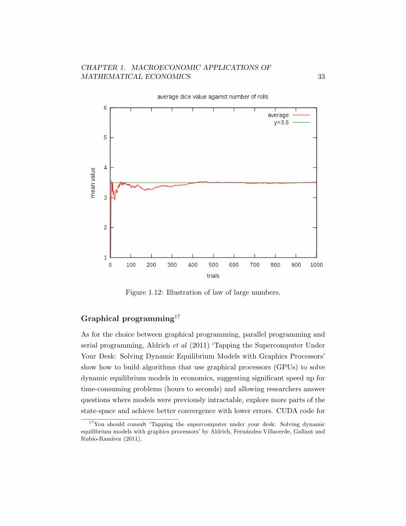
The law of large numbers states that the average of the results from a

large number of trials should be close to the expected value and will tend to

become closer as more trials are performed. See figure 1.12 for an example

for rolling a dice. With six possible outcomes {1, 2, 3, 4, 5, 6}, the mean value

is 1+2+3+4+5+66 = 3.5, towards which is what we tend to see the average of

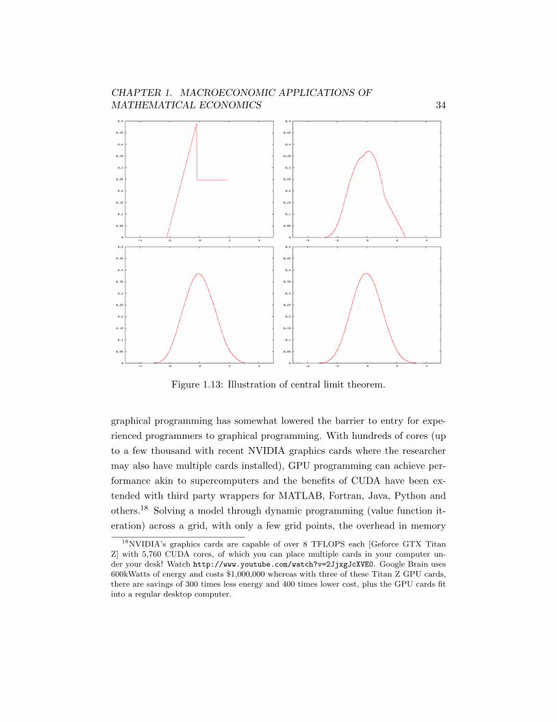
a large number of throws converging. The central limit theorem states that

for a sufficiently large number of draws of random variables, the resulting

distribution from the draws will be approximately normal irrespective of the

underlying distribution for the original random variables. See figure 1.13 for

an illustration of the distribution becoming smoother and tending towards

a Normal distribution as we sum over more and more variables. Numerical

simulation techniques make use of laws of large numbers (there are various laws

depending on what we can assume about the data) and central limit theorems

(there are multiple theorems for specific cases of what we can assume about

the data, e.g. whether the sequence of the random variables is independent

or not).

16Some other advanced topics in mathematical economics include learning in macroe-conomics, e.g. Bayesian learning (updating) and other deviations from rationality, e.g.bounded rationality.


Figure 1.12: Illustration of law of large numbers.

Graphical programming17

As for the choice between graphical programming, parallel programming and

serial programming, Aldrich et al (2011) ‘Tapping the Supercomputer Under

Your Desk: Solving Dynamic Equilibrium Models with Graphics Processors’

show how to build algorithms that use graphical processors (GPUs) to solve

dynamic equilibrium models in economics, suggesting significant speed up for

time-consuming problems (hours to seconds) and allowing researchers answer

questions where models were previously intractable, explore more parts of the

state-space and achieve better convergence with lower errors. CUDA code for

17You should consult ‘Tapping the supercomputer under your desk: Solving dynamicequilibrium models with graphics processors’ by Aldrich, Fernandez-Villaverde, Gallant andRubio-Ramırez (2011).


Figure 1.13: Illustration of central limit theorem.

graphical programming has somewhat lowered the barrier to entry for expe-

rienced programmers to graphical programming. With hundreds of cores (up

to a few thousand with recent NVIDIA graphics cards where the researcher

may also have multiple cards installed), GPU programming can achieve per-

formance akin to supercomputers and the benefits of CUDA have been ex-

tended with third party wrappers for MATLAB, Fortran, Java, Python and

others.18 Solving a model through dynamic programming (value function it-

eration) across a grid, with only a few grid points, the overhead in memory

18NVIDIA’s graphics cards are capable of over 8 TFLOPS each [Geforce GTX TitanZ] with 5,760 CUDA cores, of which you can place multiple cards in your computer un-der your desk! Watch http://www.youtube.com/watch?v=2JjxgJcXVE0. Google Brain uses600kWatts of energy and costs $1,000,000 whereas with three of these Titan Z GPU cards,there are savings of 300 times less energy and 400 times lower cost, plus the GPU cards fitinto a regular desktop computer.

http://www.youtube.com/watch?v=2JjxgJcXVE0


transmission for CUDA does not make it optimal relative to standard CPU

programming. However, as we increase the grid size, running time on CPU

tends to increase linearly while the running time with CUDA programming

on GPUs increases very slowly. In the example given in the paper, for 16 grid

points, it takes 0.03 seconds for the total CPU solution but 1.42 seconds with

the GPU solution, whereas for 65,356 grid points, it takes 24,588.5 seconds for

the total CPU solution but only 48.32 seconds with the GPU solution. Given

that the number of processors on graphics cards has increased multiples since

the paper was written and given that we can use multiple cards simultane-

ously, these estimates form a conservative lower bound on the benefits of GPU

programming.

Parallel programming

Parallel programming can reduce the running time of code by using multiple

cores or multiple nodes (machines on a cluster) simultaneously for part of

the code that can be run in parallel. Gene Amdahl (designer of IBM 360

mainframe) said that any task can be split into parts that can be parallelised

and parts that cannot; serial parts: setup of problem by reading in data,

generating statistics after each iteration, etc.; parallel parts: numerical solver,

Monte Carlo, etc. Suppose we have a task of which 95% can be executed in

parallel. Even if we use an infinite number of processes on the parallel part,

we still need 5% of the original time to execute the serial part. Amdahl’s law

states that the maximum speed up is given by the formula

1

S + 1−SN

where S is the proportion of the code to be executed in serial and N is the

number of processes in the parallel part; see figure 1.14. It is untrue that this

suggests that there is no point in writing code for more than 8-16 processes,

since as you run on larger problem sizes, often the serial part scales linearly

but the parallel part scales with n2 or n3. By tackling larger problems, a 95%

parallel problem can become a 99% parallel problem and eventually a 99.9%


parallel problem. Plugging in figures, a 99.9% problem on a 1024 way sys-

tem gives a 506 speedup. Of course, Amdahl’s law assumes that the parallel

part is perfectly parallelisable – it does not take into consideration the time

spent passing data between processes (overhead). Parallelism can occur in

two different places in a parallel computer system: (i) processor – low level

instruction parallelism (your compiler will try to take advantage of this); (ii)

interconnect – higher level parallelism (you the programmer need to manage

this). For shared memory systems (e.g. personal computer), OpenMP is an

application programming interface that can be used say in C, C++ or For-

tran. For distributed memory systems (e.g. cluster), MPI (Message Passing

Interface) is a computer library that is built on C or Fortran and used to

program parallel computers / clusters, etc.

Comparing programming languages in Economics19

As for the choice between computer programming languages, there are a num-

ber of issues relevant for researchers to consider: (i) computational burden in

terms of writing the code (e.g. number of lines of code, higher barrier to entry

on more low-level languages e.g. assembler/C/C++/Fortran where perhaps

certain tasks may be easier to complete in higher-level, menu-driven programs

or programs with in-built functions or packages for economics/econometrics

e.g. Stata/MATLAB/R/E-Views, increasing returns from specialisation in a

given language, etc.); (ii) code legacy (availability of plenty of code in For-

tran/MATLAB on the web vs less common languages); (iii) choice of com-

piler for compiled languages can make a difference in terms of speed (e.g.

Intel Fortran Compilers vs GNU compilers); (iv) replication of code (open

source available to all freely vs standards like MATLAB/Intel compilers and

expensive packages like IMSL for Fortran); (v) running time concerns may be

an issue for larger problems. On this last concern, the paper by Aldrich et

al (2014) provide a comparison of programmming languages for economists,

breaking the conventional ‘folk’ wisdom that Fortran is the fastest language

19You should consult http://economics.sas.upenn.edu/~jesusfv/comparison_

languages.pdf.

http://economics.sas.upenn.edu/~jesusfv/comparison_languages.pdf

http://economics.sas.upenn.edu/~jesusfv/comparison_languages.pdf


Amdahl’s Law

0

5

10

15

20

25

0 20 40 60 80 100 120

Spe

edup

Num Procs

Amdahl’s Law

80%90%95%

Figure 1.14: Amdahl’s law.


(C++ seems to be slightly faster for some problems), showing how choice of

compilers matter too. They solve the stochastic neoclassical growth model,

which is the workhorse model in economics, using value function iteration;

while more advanced solution methods such as projection and perturbation

are useful for DSGEs, value function iteration is more applicable to other gen-

eral problems in economics from game theory to econometrics, etc. They com-

pare compiled (e.g. Fortran/C++/Java) and scripted programming languages

(e.g. MATLAB/Julia/Python/Mathematica/R) along with hybrids of both;

another paper (Amador et al (2014)) investigates functional programming lan-

guages (e.g. Ocaml/Haskell). Rankings of the fastest language and compiler

in terms of run-time vary depending on whether the system is a Windows or

a Mac. C++ tends to slighly outpeform Fortran and whereas open source

compilers are faster on Mac (similar to a Linux system), the Intel compiler is

faster for Windows systems. Java and Julia come in next, about 2 to 3 times

as slow for the problem in the paper, whereas MATLAB is about 10 times

as slow; hybrid MATLAB using Mex files with C/C++ is significantly faster

to standard MATLAB, only about 1.5 times as slow as stand-alone C++.

Python is about 50 to 150 times as slow as C++, while the relative figures for

R and Mathematica are 250 to 500 and 625 to 800, respectively; significant

speed-up is achieved with hybrid R, Python and Mathematica bringing the

relative figures to between about 1.5 to 5 times as slow as C++.

Bibliography

DeJong, D. N. and Dave, C. (2011). Structural Macroeconometrics: (Sec-

ond Edition). Princeton University Press.

39

Macroeconomic Applications of Mathematical...

Documents

Transcript of Macroeconomic Applications of Mathematical...