Macro-econometric Modeling for an Oil Dependent Economy : An

1

Macro-econometric Modeling for an Oil Dependent Economy : An Instruments-Targets Approach for the UAE Economy

Ajit V Karnik

Professor in Economics, University of Mumbai Department of Economics, University of Mumbai,

Vidyanagari, Mumbai, 400098, India. Telephone: (91-22) 2652 6942

Fax: (91-22) 2652 8198 E-mail: [email protected]

&

Cedwyn Fernandes Associate Professor in Economics, University of Wollongong in Dubai

P.O Box 20183, Dubai, U.A.E. Tel: +9714 3672441 Fax: +9714 3672754

Email : [email protected]

Keywords: Macro-econometric models, oil dependent economies, United Arab Emirates

Economy, Instruments-Targets Approach.

This study constructs a macro-econometric model to analyze the problems of regions that exhibit dependence on non-renewable resources (e.g. oil). The role of the oil sector in the UAE and the extent to which it subsidizes the rest of the economy is evaluated. The macro-econometric model constructed consists of four sectors, has 25 equations and is evaluated and calibrated employing dynamic simulation techniques. Counter-factual and policy experiments are carried out and the instruments-targets approach is used to analyze the impact of the oil sector. The paper highlights the continued dependence of the UAE economy on oil and the urgency to diversify the economy and securing more non-hydrocarbon sources of revenue.

2

MACROECONOMETRIC MODELLING FOR AN OIL DEPENDENT ECONOMY: AN INSTRUMENTS-TARGETS APPROACH FOR THE UAE ECONOMY

Ajit V Karnik

Professor in Economics, University of Mumbai Department of Economics, University of Mumbai,

Vidyanagari, Mumbai, 400098, India. Telephone: (91-22) 2652 6942

Fax: (91-22) 2652 8198 E-mail: [email protected]

&

Cedwyn Fernandes* Associate Professor in Economics, University of Wollongong in Dubai

P.O Box 20183, Dubai, U.A.E. Tel: +9714 3672441 Fax: +9714 3672754

Email: [email protected]

3

* Author to be contacted for questions

4

1. INTRODUCTION

The United Arab Emirates (UAE) is a federation formed in 1971 and comprises the seven emirates: Abu Dhabi, Ajman, Dubai, Fujairah, Ras Al-Khaimah, Sharjah and Umm Al-Qaiwan. Each constituent of the federation retains considerable degree of economic and political autonomy. It is, of course, well known that the UAE is oil-rich even though all the emirates are not as well endowed. However, each emirate retains full ownership and control over its oil resources (Ahmed and Mottu, 2002).

The transformation of the UAE from an economy precariously based on fishing and pearling to an oil-based, high-income economy over the last three decades has been spectacular. As important have been the concerted efforts to make the economy of the UAE less dependent on oil and towards making it more diversified. In fact, the pace of reduction in oil dependency has been fastest in the UAE as compared to other GCC countries. The ratio of oil revenue to total government revenue has declined in the UAE from 90% in 1980 to 50-60% by 2004; in contrast, the decline in other GCC countries has been more muted (IMF, 2005). This decline has been made possible by actively developing the non-oil sector of the economy. The non-oil sector has been liberalized in recent years and this has fostered its rapid expansion as well as ushering in the private sector. Thus the diversification of the economy has been driven by the rapid expansion of services such as tourism, finance, transport and communication.

This paper is concerned with developing a detailed macroeconometric model of the UAE economy essentially with a view to understanding its functioning. Macroeconometric modeling has a venerable lineage beginning with Tinbergen (1956). Following in his footsteps, numerous scholars have contributed to modeling a quintessential developing economy, namely, India (see, Krishnamurty 2002 for a survey). However, there has not been as much attention paid to countries that exhibit dependence on a non-renewable resource, such as oil. The problems of these countries are of a different order from the traditional approaches to macro modeling. While the traditional approach needed to distinguish between a forward-looking (urban) sector and a traditional (rural) sector, for oil-rich countries the distinction is between the oil and the non-oil sector of the economy.

There have been attempts at explaining the performance of the UAE economy taking into account its dependence on oil. See, for instance, Elhiraika and Hamed (2002) who examine growth in the federation. The approach however is not economy wide, in the sense of a macro model. The study is in a growth accounting framework and tries to identify the sources of growth. However, it is not apparent from the study as to what is the level of dependence on the oil sector. Fasano and Wang (2001) seek to examine the performance of the non-oil sector and relate it specifically to the fiscal expenditure policy. A completely different approach characterizes Ahmed and Mottu (2002) who are concerned with assignment of oil revenues to subnational governments. The authors investigate the sharing of oil revenues for a large number of federations including the UAE.

In spite of increasing attention to the analyzing the economic problems of oil rich economies such as the UAE, we have not come across a rigorous macroeconomic approach. It is our belief that the issues tackled in Elhiraika and Hamed (2002) and Fasano and Wang (2001) can be subsumed in the context of a macroeconometric model. Our model will view the oil and non-oil sectors of the UAE economy separately. At the same time, it will also look at, in a disaggregated manner, revenue generation by the government from the two sectors. Such an approach, we believe will enhance our understanding of the fiscal operations of the government.

5

Simultaneously, we will be able obtain insights into the crucial question as to if and to what extent the oil sector “subsidizes” the non-oil sector of the economy.

The plan of the paper is follows: Section 2 develops the macroeconometric model of the UAE economy. Section 3 presents the dynamic simulation of the model. Section 4 presents the results of the structural analysis of the model. Counter-factual experiments are presented in section 5. Section 6 develops a proto-type model for operationalising Tinbergen’s instruments-targets approach. Section 7 concludes. 2. MACROECONOMETRIC MODEL OF THE UAE

We develop a twenty-five equations model of the UAE economy. The economy has been divided into four sectors: Output Sector, Government Sector, Monetary Sector and External Sector. The model consists of eleven behavioural equations and fourteen accounting identities. The abbreviations employed for each variable have been listed in Tables 1-A, 1-B and 1-C.

TABLE 1-A: LIST OF ENDOGENOUS VARIABLES

1. CB Current Balance (million dirham) 2. GFD Gross Fiscal Deficit (million dirham) 3. CE Current Expenditure (million dirham) 4. GDCFC Real Gross Domestic Capital Formation (million

dirham) 5. GDPC Real GDP (million dirham) 6. GDPN Nominal GDP (million dirham) 7. HCR Hydrocarbon Revenue (million dirham) 8. INV Investment Income (million dirham) 9. M1 Money Supply (million dirham) 10. MC Real Imports (million dirham) 11. MN Nominal Imports (million dirham) 12. NGDPC Real Non-oil Sector GDP (Obtained by subtracting

GDP from mining sector) (million dirham) 13. NGDPN Nominal Non-oil Sector GDP (Obtained by

subtracting GDP from mining sector) (million dirham)

14. NHB Non-hydrocarbon Balance (million dirham) 15. NHCR Non-hydrocarbon Revenue (million dirham) 16. OGDPC Real Oil Sector GDP (million dirham) 17. OGDPN Nominal Oil Sector GDP (million dirham) 18. P GDP Deflator (Base Year 1990) 19. ST Subsidies and Transfers (million dirham) 20. TAX Taxes, including customs, profit transfers, income

tax, fees and charges and other revenue (million dirham)

21. TEG Total Expenditure and Grants (million dirham)

6

22. TR Total Revenue (million dirham) 23. WS Wages and Salaries (million dirham) 24. XC Real Exports (million dirham) 25. XN Nominal Exports (million dirham)

TABLE 1-B: LIST OF POLICY VARIABLES

1. ADFS Abu Dhabi Federal Services (million dirham) 2. DE Development Expenditure (million dirham) 3. FG Foreign Grants (million dirham) 4. GDCFN Nominal Gross Domestic Capital Formation (million

dirham) 5. GS Govt Expenditure on Goods and Services (million

dirham) 6. LE Govt Expenditure on Loans & Equity (million

dirham) 7. OTHREXP Other Govt Expenditure (million dirham) 8. OUAE Oil Production in UAE (sum of average monthly

production measured in thousand barrels per day)

TABLE 1-C: LIST OF EXOGENOUS VARIABLES

1. CB(-1) Lagged Current Balance (million dirham) 2. NGDPC(-1) Lagged Real Non-oil Sector GDP (million dirham) 3. P(-1) Lagged GDP Deflator (base year 1990) 4. ASIA Dummy Variable = 1 in 1997

0, otherwise 5. DUM Dummy Variable = 1 in 1998

0 otherwise 6. OIL World Oil Prices ($s per barrel) 7. PG Deflator for Gross Domestic Capital Formation (base

year 1990) 8. PM Deflator for Imports (base year 1990) 9. PN Deflator for Non-oil Sector GDP (base year 1990) 10. PO Deflator for Oil Sector GDP (base year 1990) 11. PX Deflator for Exports (base year 1990) 12. TIME Trend Variable 13. TWER USA’s Trade Weighted Exchange Rate (1997=100) 14. USKTR Real USA Stock Prices 15. WIR World Interest Rate (US Fed Fund Rate) (%)

We now present the model along with a discussion of each equation and the rationale

underlying its specification. It may be noted that, despite the known inappropriateness of OLS for estimating structural form equations, we have used this technique. Given the short time series that was available to us, we felt it prudent to not impose the weight of sophisticated techniques

7

such as Two Stage Least Square or Three Stage Least Squares on the data set that we had. Our motivation in this was that the data must stand the weight of the techniques. Further, even for the innumerable macroeconometric models that have been estimated for India, the OLS technique has been used even when the number of observations has been double than what we have for the UAE (See, Rao 1987 or Krishnamurthy, 2002). Output Sector

The economy of UAE is divided into two components: oil producing sector and non-oil producing sector. Real GDP originating in the oil- producing sector (OGDPC) is governed by the oil output in the region (OUAE) and world oil prices (OIL). In addition, the demand side is captured by gross fiscal deficit (GFD). Remembering that deficits are defined as revenues minus expenditures, a negative value for GFD indicates a deficit and a positive value indicates a surplus. Hence, a unit fall in GFD i.e. an increase in gross fiscal deficit will boost demand and result in higher OGDPC. Equation (1) gives the details. OGDPC = -15428 + 1.4839*OUAE + 1798.5*OIL -0.2855*GFD (-2.02) (6.42) (8.86) (-2.48)

(1)

R-SQUARE ADJUSTED = 0.8700 DURBIN-WATSON = 1.91

The non-oil sector of the economy is now modeled. GDP from this sector (NGDPC) is specified in a partial adjustment framework with lagged NGDPC, real gross domestic capital formation (GDCFC) and government spending on wages and salaries (WS). In addition, we have introduced a dummy variable to capture prices of oil in 1998. Oil prices in the decade of the 1990s have been generally lower than in the 1980s; further, all through the 1990s, oil prices have been declining and the lowest level was attained in 1998: prices were as low as $12 a barrel. Consequently, with oil prices dipping and OGDPC (which has oil prices as an explanatory variable) being adversely affected, it was expected that the non-oil sector would compensate for this decline. The dummy variable (DUM) is designed to capture this effect on NGDPC. Equation (2) reports the results. NGDPC = 8665.9 + 0.2726*NGDPC(-1) + 0.3654*GDCFC + 3.3137*WS (2.88) (2.01) (2.79) (5.26) +5747.2*DUM (2.34) (2) R-SQUARE ADJUSTED = 0.9820 DURBIN H STATISTIC (ASYMPTOTIC NORMAL) = -1.4482

In addition to the two behavioural equations given above, this sector consists of some definitional identities as well as identities that allow us to move from real quantities to nominal

8

quantities. First, in equation (3) we express real GDP (GDPC) as the sum of GDP originating in the oil sector (OGDPC) and the non-oil sector (NGDPC). GDPC = OGDPC + NGDPC (3)

Nominal GDP is required in some of the equations that we report later. Hence, equation (4) links nominal GDP (GDPN) to real GDP(GDPC) via the GDP deflator (P). GDPN = P*GDPC (4)

Likewise, in equation (5) we link nominal oil sector GDP (OGDPN) to real oil sector (OGDPC) via the price deflator for this sector (PO). Equation (6) does the same for the non-oil sector. OGDPN = PO*OGDPC (5) NGDPN = PN*NGDPC (6) Government Sector

This sector is the most detailed of all the sectors of the model. Of the twelve equations in this sector, four are behavioural equations and the rest are identities. Of the total non-hydrocarbon revenue collected (ignoring investment income, which is modeled separately), taxes, namely, customs and incomes tax are the most important. Hence, we model tax revenues (TAX) in a simple form as being determined by nominal non-oil sector GDP (NGDPN) (equation 7). TAX = -10567 +0.2413*NGDPN (7) (-8.41) (15.61) R-SQUARE ADJUSTED = 0.9625 DURBIN-WATSON = 1.9701

Revenues from the hydrocarbon sector (HCR) are determined by the output levels in the oil sector of the GDP (OGDPN). We also noted that the year 1998 show a sharp drop in HCR, which is attributable to the low world oil prices prevailing in that year. We capture this effect using a dummy variable (DUM). Equation (8) reports the estimation. HCR = -3650 + 0.6353*OGDPN - 10698*DUM (8) (-0.94) (9.48) (-2.04) R-SQUARE ADJUSTED = 0.7661 DURBIN-WATSON = 1.9350

9

Government expenditures on wages and salaries (WS) reflect the key role played by the federal government to provide employment to Emirati nationals, particularly from the poorer northern Emirates (IMF, 2003). It also reflects the efforts to hire teachers and health workers to keep pace with the increase in population. We model WS as a function of the levels of Current Expenditures (CE) of the government. It is also true that the government is engaged in a lot of welfare activities and it may be argued that WS is one such. However, given limited resources the various welfare activities of the government are in competition with one another. Specifically, we argue that the Subsidies and Transfers (ST) are in a competitive relationship with WS, so that the coefficient attached to ST should be negative. The resources required for funding WS are on both hydrocarbon and non-hydrocarbon revenues. It would be expected that the very low world prices of oil would affect WS. We introduce a dummy variable (DUM) to capture this effect. Equation (9) reports the results. WS = 1167.5 + 0.2673*CE - 0.2899*ST -861.38*DUM (2.04) (14.61) (-8.57) (-2.89)

(9) R-SQUARE ADJUSTED = 0.9700 DURBIN-WATSON = 1.7015

Current balances (CB), the matching of current revenues and current expenditures of the government, has been modeled as a behavioural equation rather than identity. We do this mainly to endogenize current expenditures as well as to capture the fact that CB have been deteriorating over the years. The equation for CB is specified in a partial adjustment framework. In addition, we include total revenues (TR) as an explanatory variable while the secular worsening of CB is captured by including a trend variable (TIME). Equation (10) reports the results. CB = 5966.3 -0.2409*CB(-1) +0.8102*TR -2505.8*TIME (1.17) (5.83) (-5.97)

(10) R-SQUARE ADJUSTED = 0.6947 DURBIN H STATISTIC (ASYMPTOTIC NORMAL) = -1.6971

Total Revenues (TR) come from both tax and non-tax sources. However, we prefer to model as originating from hydrocarbon (HCR) and non-hydrocarbon (NHCR). Equation (11) reports this identity. TR = HCR + NHCR (11)

As stated earlier, we have preferred to write current expenditures (CE) as an identity rather than current balance (CB). Equation (12) reports CE as the difference between total revenues (TR) and current balance (CB). CE = TR – CB (12)

10

Apart from the current balance, we also model overall budget balance i.e. gross fiscal deficit (GFD) as the gap between total revenues (TR) and total government expenditures (TEG). Equation (13) reports this identity. GFD = TR – TEG (13)

For oil-rich economies, non-oil fiscal balance is a better indicator of underlying fiscal trends than the traditional overall fiscal balance since it abstracts from the volatility of oil prices and revenues (IMF, 2003). We model non-fiscal balance or non-hydrocarbon balance (NHB) as the gap between non-hydrocarbon revenues (NHCR) and total expenditures (TEG). This identity is given in equation (14). NHB = NHCR – TEG (14)

There exist two avenues for garnering non-hydrocarbon revenues (NHCR), namely, income from investment made abroad (INV) and taxes raised domestically (TAX). This is shown in equation (15). NHCR = INV + TAX (15)

Equation (16) reports total expenditures (TEG) as a sum of current expenditures (CE), development expenditures (DE), loans and equity (LE) and foreign grants (FG). TEG = CE + DE + LE + FG (16)

We model subsidies and transfers (ST) as a residual after subtracting wages and salaries (WS), government expenditures on goods and services (GS), expenditure on Abu Dhabi federal services (ADFS), which are mainly defense and internal security outlays, and other expenditures (OTHREXP). The main rationale for this identity (equation 17) is to once again show the competitive relationship between ST and WS, just as we had done in equation (9) for WS. ST = CE – WS - GS - ADFS - OTHREXP (17)

The final equation in this sector relates real gross domestic capital formation (GDCFC) to nominal gross domestic capital formation (GDCFN) via the deflator for capital formation. The reason for introducing equation (18) is that, in our policy experiments, we shall be using nominal capital formation as a policy variable. The rationale for this is that, of the total capital formation in any economy, government capital formation accounts for a significant proportion via development expenditures. Further, government’s development expenditures act as a signal to private investors to increase their own investment. If one assumes “crowding in” with respect to government capital formation, governments can, indeed, control total capital formation in the economy. Governments, however, can only fix the level of a policy variable in nominal terms; its real values are determined by the level of prices, which, of course, cannot be set at a level desired by the government.

11

GDCFC = GDCFN/PG (18) Monetary Sector

Two equations comprise the monetary sector. In the first, we model money supply (M1) as being determined by gross fiscal deficit (GFD) and inflows of foreign exchange via nominal exports (XN). Since GFD is defined as Revenue minus Expenditures, a negative GFD indicates a deficit. Hence, the coefficient of GFD is expected to be negative. A rise in GFD will require to debt creation some of which will be subscribed to by the central bank thereby raising money supply. Equation (19) reports the results of estimating this equation. M1 = - 3364.2 - 0.1710*GFD + 0.2412*XN (19) (-1.02) (-2.70) (6.94) R-SQUARE ADJUSTED = 0.9050 DURBIN-WATSON = 1.658

Prices (P) as depicted by the GDP deflator are modelled in a partial adjustment framework with lagged P as a right-hand side variable. Apart from this we introduce, money supply (M1) and import prices (PM) as explanatory variables. Equation (20) reports the results. P = 0.0358 + 0.4175*P(-1) + 0.0000068*M1 +0.4587*PM (0.19) (2.17) (3.16) (2.57)

(20) R-SQUARE ADJUSTED = 0.9715 DURBIN H STATISTIC (ASYMPTOTIC NORMAL) = -0.5984 External Sector

The external sector consists of four equations, of which two are behavioural equations. The first of the behavioural equation models investment income (INV) as being determined by the real returns on the stock market in the USA (USTKR) and world interest rates (WIR). In addition, we expect that the Asian currency crisis of 1997 dented world confidence, which eroded returns from investments. This is captured by a dummy variable that we call ASIA. Equation (21) reports the results of estimating INV. INV = 2856.1 + 6.7581*USTKR + 1461.6*WIR -2726.8*ASIA (1.26) (3.84) (7.47) (-1.42)


12

Nominal exports (XN) are expected to be positively associated with nominal GDP (GDPN) but negatively associated with domestic prices (P). Higher domestic prices will make exported goods more expensive and not as competitive in the world markets. Low world oil prices in 1998 lowered export earnings. This is captured by a dummy variable (DUM). Equation (22) reports results. XN = 36572 + 1.0080*GDPN -81238*P -4443.7*DUM (1.75) (11.54) (-2.75) (-2.69)


Nominal imports (MN) are determined by nominal GDP (GDPN), trade weighted exchange rate of the USA (TWER) and gross fiscal deficit (GFD). It’s obvious that GDPN will have a positive impact on MN. The currency of UAE is pegged to the US dollar. Hence, any changes in the US dollar will have concomitant effect on the UAE dirham. The TWER for the USA is an index that measures the number of US dollars to be paid for a weighted basket of foreign currencies. Depreciation in the currency is reflected in a rise in the index. It is, of course, clear that depreciation makes imports more expensive and, hence, a rise in TWER will lead to lower MN. A rise in GFD implies an increase in domestic demand for all goods, including imported goods. Remembering that we are measuring a deficit as TR minus TEG, the sign associated will be negative i.e. a fall in deficits will raise imports. Equation (23) reports the results. MN = -4804 + 0.8049*GDPN -313.93*TWER -0.3763*GFD (-0.48) (16.00) (-2.34) (-2.07)


The next two identities link real exports (XC) to nominal exports (XN) via a deflator for exports (PX) (see equation 24). Equation 25 links real imports (MX) to nominal imports (MN) via a deflator for imports (PN). XC = XN/PX (24) MC = MN/PM (25) 3. EVALUATION OF THE MODEL: DYNAMIC SIMULATION

The best way to evaluate the model estimated in the previous section is to carry out a dynamic simulation. In a dynamic simulation as opposed to static simulation, solved values of lagged endogenous variables are used in place of actual values. This effectively means that any errors in the simulation of the profiles of endogenous variables percolate through the model via the lagged values of these variables. It may be remembered that our model had three lagged

13

endogenous variables, namely, lagged current balance (CB(-1), lagged nominal non-oil GDP (NGDPN(-1)) and lagged prices (P(-1)). The difference between static and dynamic simulations makes it obvious that simulation performance of the latter cannot be superior to that of the former. In spite of this danger of obtaining a weaker simulation performance under dynamic simulation, we have preferred to stay with it since it gives a better evaluation of the model than does static simulation.

We shall be evaluating simulation performance using a variety of criteria: a) Root mean square percent error (RMSPE) defined as:

100*])[( 2

TASA

RMSPE ttt∑ −=

where, At = Actual value of the endogenous variable St = Simulated value of the endogenous variable T = Number of time periods over which simulation is carried out

b) The correlation between the actual and simulated values of the endogenous variable is

computed. Obviously, the higher this correlation, the better is the simulation performance. c) Apart from the above two criteria, quality of simulation can also be judged by the ability of

the simulated profile of the endogenous variable to capture the turning points in the actual profile of the variable. This can best be seen by plotting the actual and simulated values of the endogenous variable. However, in the interest of conserving space, we do not report the plots for all the endogenous variables but report them only for those variables for which the first two criteria show a poor performance. We carry out dynamic simulation over the period 1991 to 2001 and Table 2 reports the

RMSPEs and correlation coefficients for all the endogenous variables.

TABLE 2: SIMULATION PERFORMANCE

Endogenous Variable

RMSPE (%)

Correlation Between Actual and Simulated

Values OUTPUT SECTOR OGDPC 10.94 0.64 NGDPC 7.18 0.89 GDPC 7.82 0.85 GDPN 8.19 0.91 OGDPN 10.94 0.87 NGDPN 7.18 0.95 GOVERNMENT SECTOR TAX 21.08 0.89 HCR 19.78 0.82 WS 12.99 0.84

14

CB 187.88 0.24 TR 12.48 0.90 CE 11.38 0.96 GFD 104.75 0.51 NHB 13.59 0.87 NHCR 10.33 0.94 TEG 7.46 0.94 ST 117.35 0.52 GDCFC 0.00 1.00 MONETARY SECTOR M1 9.88 0.98 P 3.16 0.94 EXTERNAL SECTOR INV 12.02 0.96 XN 13.77 0.89 MN 11.16 0.87 XC 13.77 0.88 MC 11.16 0.86

The simulation performance for most equation is good either according to the RMSPE

value or the value of the correlation coefficient or both. However, there are three variables, which have been highlighted in Table 2, which do not exhibit a good simulation performance. For these variables we shall present plots of their actual and simulated values to examine if the simulation is able to capture the turning points in the actual series.

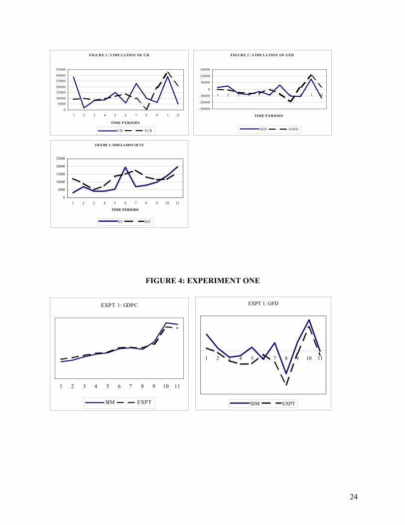
In Figure 1, we plot the actual and simulated profiles of CB. While the performance is not as good as some of the other variables, it does not reflect the poor fit indicated by the RMSPE. The direction of movement of the simulated series captures reasonably well the actual series.

Figure 2 plots the actual and simulated values of GFD. Once again we notice that the turning points of the actual series are captured by the simulated series.

Finally, in Figure 3 we plot the simulated and actual values of the third series that exhibited a poor simulation performance as per its RMSPE and the correlation coefficient reported in Table 2. The plots in Figure 3 indicate that ST is, indeed, the endogenous variable that shows a simulation performance that is worse than all the other variables. However, even for this variable, a case can be made that, albeit only weakly, the simulated series does capture the directionality of the original series. 4. STRUCTURAL ANALYSIS OF THE MODEL

A very useful procedure for investigating whether the estimated and simulated model incorporates the expected causalities between the policy/exogenous variables is to obtain the impact multipliers of the model. The impact multipliers, as is well known, are obtained from the reduced from of the estimated model. However, if the model contains non-linearities, it is not straightforward to obtain the reduced form. The model has to be, perforce, linearized before its reduced form becomes available. Non-linearities are present in the model being used in this

15

paper via equations (4), (5), (6), (18), (24) and (25). We have employed the so-called operating point method (Rao, 1987) to linearize the model around reference values for each variable – endogenous, policy and exogenous – in the model. Deviations of second and higher order are ignored and we end up with a time-invariant transfer function. In our linearization exercise, the reference values selected were the actual historical values taken by all the variables in the year 1990. We shall demonstrate the procedure for linearizing one of the non-linear equations in the model, but not present the entire linearized model. Consider equation (4) which is reproduced below: GDPN = P*GDPC

Each variable in the above equation is replaced by its reference value, denoted by writing the variable in small case plus the deviation from it, denoted by d. gdpn + dGDPN = (p + dP)(gdpc + dGDPC)

Expanding out the expression on the right hand side of the equation above: gdpn + dGDPN = p*gdpc + p*dGDPC + gdpc*dP + dP*dGDPC

Remembering that the deviations of second and higher order are ignored and that we have used as reference values the historical values of the variables in the year 1990, we have: 124008 + dGDPN = 1*124008 + 1*dGDPC + 124008*dP

The year 1990 is the base year and hence nominal and real values are equal and the GDP deflator (P) takes on a value of 1. Simplifying the above equation yields: dGDPN = dGDPC + 124008*dP

This procedure has been used to linearize all the equations in the model after which the linearized version was used to obtain the reduced form. In the interest of conserving space, we shall present the impact multipliers of only a select policy and exogenous variables. In Table 3, we present the impact of multipliers of some policy variables on some of the endogenous variables.

16

TABLE 3: IMPACT MULTIPLIERS OF SOME POLICY VARIABLES

OUAE DE GDCFN OUTPUT SECTOR

OGDPC 1.2901 0.2482 -0.0181 NGDPC 0.0754 0.0145 0.3725 GDPC 1.3655 0.2627 0.3543

GOVERNMENT SECTOR TAX 0.0182 0.0035 0.0899 HCR 0.8196 0.1577 -0.0115 WS 0.0228 0.0044 0.0021 CB 0.6788 0.1306 0.0635 TR 0.8378 0.1612 0.0784 CE 0.1590 0.0306 0.0149 GFD 0.6788 -0.8694 0.0635 NHB -0.1408 -1.0271 0.0750 NHCR 0.0182 0.0035 0.0899 TEG 0.1590 1.0306 0.0149 ST 0.0681 0.0131 0.0064

MONETARY SECTOR M1 0.4827 -0.0913 0.1045

EXTERNAL SECTOR XN 1.5201 0.2376 0.3883 MN 1.1793 0.4775 0.3342

The significance of the oil sector is seen from the impact multipliers associated with

OUAE, the variable denoting oil production in the country. A unit increase in oil production raises OGDPC by 1.29 million dirham. Likewise there is great improvement in HCR, CB and GFD while at the same enabling the government to carry out higher levels of expenditure. Increases in DE also have beneficial effect on the economy in terms of higher output. However, the impact on the government sector is mixed: CB improves, but GFD and NHB deteriorate significantly. While the positive impact of increases in OUAE and DE was the strongest on OGDPC, an increase in GDCN benefits the non-oil sector: NGDPC increases. The impact on the government sector is minimal. Even though we do not report the results, it may be noted that, for the policy variables reported in Table 3, the impact on prices was negligible. The structure of the price equation in the model is such that the links between prices and the policy variables is tenuous at best.

In Table 4, we present the impact of multipliers of some exogenous variables on some of the endogenous variables.

17

TABLE 4: IMPACT MULTIPLIERS OF SOME EXOGENOUS VARIABLES

OIL USTKR WIR OUTPUT SECTOR

OGDPC 1563.6212 -1.3892 -300.4575 NGDPC 91.3834 0.5405 116.8979 GDPC 1655.0046 -0.8487 -183.5596

GOVERNMENT SECTOR TAX 22.0508 0.1304 28.2075 HCR 993.3686 -0.8826 -190.8806 WS 27.5775 0.1631 35.2771 CB 822.6928 4.8660 1052.3905 TR 1015.4194 6.0059 1298.9268 CE 192.7266 1.1399 246.5363 GFD 822.6928 4.8660 1052.3905 NHB -170.6758 5.7486 1243.2711 NHCR 22.0508 6.8885 1489.8075 TEG 192.7266 1.1399 246.5363 ST 82.5746 0.4884 105.6296

MONETARY SECTOR M1 585.0544 0.6741 145.7947

EXTERNAL SECTOR INV 0.0000 6.7581 1461.6000 XN 1842.3463 -0.6549 -141.6422 MN 1429.2987 -2.0579 -445.0785

World price of oil (OIL) is seen to be such an important variable in terms of its effect on

all sectors of the economy. For instance, a unit increase in OIL raises GDPC by 1655 million dirhams. The only negative impact of an increase in OIL is on NHB, the reason for it being that, even though NHCR rises, TEG rises even faster leading to a worsening of the NHB. As is to be expected, an increase in USTKR has the greatest positive impact on INV leading to a beneficial impact on CB, GFD and NHB. However, its impact on the output sector is negative as, indeed, it is of an increase in WIR. Even in the case of an increase in WIR, there is an improvement in the fiscal balances even though the impact on output is negative. Prices (P) are significantly affected by an exogenous variable, namely, imported prices (PM), not reported in Table 4. The impact multiplier of P with respect to PM is as high as 0.4942. Prices are also affected by, as would be expected, prices in the oil sector (PO) and the non-oil sector (PN). The associated impact multipliers are 0.0256 and 0.0106, respectively.

18

5. COUNTER-FACTUAL EXPERIMENTS A macroeconometric model that has been well-specified, that simulates well and satisfies

expected causal relationships as exhibited by impact multipliers may be used to conduct certain counter-factual experiments. We conduct the following experiments over the period 1991 to 2001 and examine the effect some policy variables – known as instruments - have on a few select endogenous variables – known as targets: 1. Experiment 1: Development expenditure (DE) is clearly an instrument in the hands of a

government seeking to attain certain targets. We assume that DE rises 20% above its historical profile.

2. Experiment 2:Gross domestic capital formation (GDCFN) is also one more instrument variable and we assume that it rises 20% above its historical profile.

3. Experiment 3: World oil prices (OIL) rise 20% above their historical profile. We realize that world oil prices are not set by the UAE and, in that sense, OIL cannot be an instrument of policy. However, given that the UAE is a member of OPEC, it could, conceivably co-ordinate its actions with other members in order to raise prices.

4. Experiment 4: Domestic production of crude oil (OUAE) is clearly an instrument of policy. However, it is quite likely that, as oil reserves get depleted, production of crude oil will reduce over time. We design an experiment such that, in the terminal year of our experiment period, production is 25% below the historical level.

Experiment 1

For all the experiments, we compare the experimental paths of the target endogenous variable with its simulated paths. For all the experiments, we focus on four target variables even though results are available for all. These four variables are:

1. GDP at constant prices (GDPC) 2. Gross Fiscal Deficit (GFD) 3. Non-hydrocarbon fiscal balance (NHB) 4. Government expenditure on subsidies and transfers (ST).

The experimental and simulated of the above variables are given in the graphs (Figure 4) on the next page. Over the entire period of the experiment, we have computed the changes in the experimental path vis-à-vis the simulated and computed the gains and losses over the entire period. This is a simple way of discerning if the experiment results in an improvement in the variable. For the entire period we found:

• Experimental GDPC was greater than the simulated GDPC by only 0.32%. It may be noted that experimental oil-sector GDPC (OGDPC) was higher by 1.56% and NGDPC was lower by 0.55%.

• Experimental GFD is worse by more than 350%, while current balance (CB) worsens by only 16%.

• Experimental NHB improves by almost 15%. • Expenditure on ST increases by 1.8%. Simultaneously, expenditures on wages and

salaries (WS) falls by 0.79%.

19

Experiment 2

The experimental and simulated of the select variables are given in Figure 4. We also give the gains and losses over the entire period of the experiment. For the entire period we found:

• Experimental GDPC was greater than the simulated GDPC by 2.19%. It may be noted that experimental oil-sector GDPC (OGDPC) was higher by 0.31% and NGDPC was higher by 3.19%.

• Experimental GFD is worse by 188%, while current balance (CB) worsens by only 15%. • Experimental NHB improves by almost 6%. • Expenditure on ST increases by almost 3%. Simultaneously, expenditures on wages and

salaries (WS) falls by 0.83%.

Experiment 3


• Experimental GDPC was greater than the simulated GDPC by almost 4%. It may be noted that experimental oil-sector GDPC (OGDPC) was higher by 10.5% and NGDPC was lower by 0.75%.

• Experimental GFD is worse by 10%, while current balance (CB) worsens by less than 1%.

• Experimental NHB improves by almost 12%. • Expenditure on ST increases by almost 13%. Simultaneously, expenditures on wages and

salaries (WS) falls by 1%. Experiment 4


• Experimental GDPC was lower than the simulated GDPC by 4.5%. It may be noted that experimental oil-sector GDPC (OGDPC) was lower by almost 11% and NGDPC was marginally lower.

• Experimental GFD is worse by an enormous 480%, while current balance (CB) worsens by almost 40%.

• Experimental NHB improves by 3.5%. • Expenditure on ST declines by 13%. Simultaneously, expenditures on wages and salaries

(WS) falls by less than 1%.

The major result to emanate from our policy experiments is the importance of crude oil in the UAE economy. This is clearly seen in the context of a rise in world oil prices. The real sector experiences a boost in the growth rate, while there is a beneficial impact or, at worst, no impact on government operations. Even more worryingly, the adverse consequences of a decline in crude oil production are very strong. Not only does real GDP declines by almost 5% but gross fiscal deficit worsens by a whopping 480%. This shows that, while diversification may insulate

20

the economy from adverse effects of oil depletion, government finances still remain critically depends on the oil sector. 6. TINBERGEN’S INSTRUMENTS-TARGETS APPROACH In the previous section we have tried to examine how changes in some policy variables, used as instruments, affect some endogenous variables, which are the targets of the government. An alternative, but a very venerable approach to policy evaluation using an estimated macroeconometric model is the instruments-targets approach to policy evaluation developed by Tinbergen (1956). The main thrust of this approach is that there exist some endogenous variables – known as targets – whose desired values are sought to be achieved by using policy variables – known as instruments. An important assumption in implementing this approach is that the number of instruments, l exceeds or equals the number of targets, g (Intriligator et al, 1996), i.e.

l ≥ g (A)

The difference (l – g) is called the policy degrees of freedom. Suppose that the structural form of the model with the dimensions of the associated

vectors/matrices is given by:

)1()()1()()1()()1()()1(

1 (B)ggllgkkgggggg

ttttt AuCzByy×××××××××

− =+++Γ ε

where, yt are the targets. yt-1 are the lagged values of the targets. zt are exogenous variables. ut are the instruments. εt are the disturbance terms Γ, B, C, and A are coefficient matrices

Assuming that the coefficient matrices in equation (B) have been estimated and assuming that the matrix A can be inverted – either by assuming that is square and non-singular or by assuming that a pseudo-inverse can be obtained if l > g – we can write the following:

(C)ˆˆˆˆˆˆˆˆ 11011

10* −−−−

− +−−Γ−= AACzAByAyu tt tttε

In equation (C), the left-hand side gives the optimal values of the target variables for desired values of the instruments. Further, from (C) we can obtain the sensitivities of the optimal values of the target variables with respect to the desired values of the targets. These sensitivities are given by:

21

(D)10

*−Γ−=

∂∂ A

yu

t

t

Instead of using the full 25 equations model, we have experimented with the instruments-

targets approach employing a proto-type 3 equations model given below. This model captures the essence of an oil-rich economy by incorporating hydrocarbon revenues (HCR) in the picture. Remembering that, in the context of the full model developed earlier in the paper, HCR is related to oil-sector GDP, which is connected to crude oil production and world oil prices, even this proto-type will yield useful insights in the working of the economy of UAE. GDPC = 39202 + 0.7495*TEG + 1.4860*GDCFC (E) (4.13) (5.83) (3.45) R – SQUARE ADJUSTED = 0.9145 DW = 1.9254 TEG = -12907 + 0.6979*CE + 0.1810*HCR + 0.2690*GDPC (-1.79) (6.55) (1.40) (2.72)

(F) R – SQUARE ADJUSTED = 0.9525 DW = 2.0801 CB = HCR + NHCR - CE (G)

The proto-type model is particularly simple in that there are no lagged dependent variables nor are there any exogenous variables. The number of targets is three – GDPC, TEG and CB – while the number of instruments is four – GDCFC, HCR, NHCR and CE. It may be recalled that all of these instruments (policy variables) were endogenised in the larger model discussed earlier. It is only in the context of this prototype model, for the sole purpose of tractability, that we designate them as instruments, realizing well that, in fact, the government can have only imperfect control over these variables. For instance, we have stated earlier that governments can control only the nominal levels of policy variables and that their levels in real terms. And, yet, tractability demanded that we work with GDCFC, real as an instrument. Clearly, in the prototype model, the number of instruments is more than the number of targets, and, hence, the coefficient matrix A (see equation (B) above) will not be square. We have, therefore, computed the pseudo-inverse of A, which when post-multiplied to -Γ will yield the sensitivities given in equation (D) above. It may be noted that, in the situation where the number of instruments is greater than the number of targets, Intriligator et al (1996) recommend setting one of the instrument at some desirable thereby rendering the A matrix square. We have not chosen to do so since we felt it is better to carry out the exercise with positive policy degrees of freedom.

22

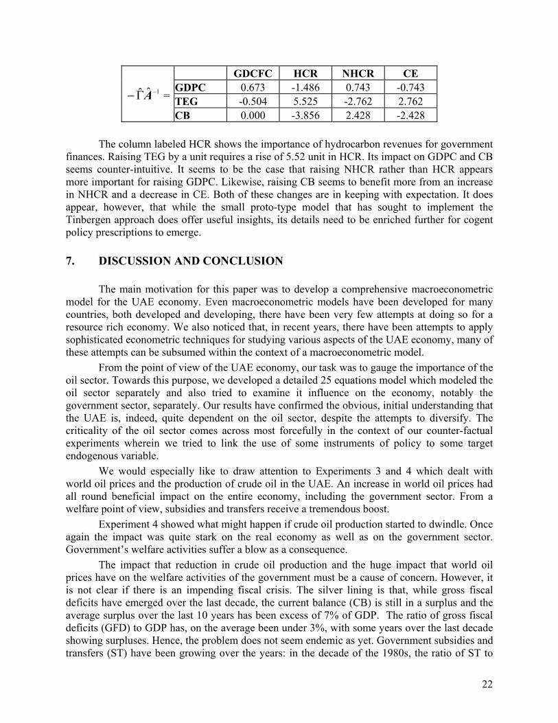
GDCFC HCR NHCR CE GDPC 0.673 -1.486 0.743 -0.743 TEG -0.504 5.525 -2.762 2.762

1ˆˆ −Γ− A =

CB 0.000 -3.856 2.428 -2.428

The column labeled HCR shows the importance of hydrocarbon revenues for government finances. Raising TEG by a unit requires a rise of 5.52 unit in HCR. Its impact on GDPC and CB seems counter-intuitive. It seems to be the case that raising NHCR rather than HCR appears more important for raising GDPC. Likewise, raising CB seems to benefit more from an increase in NHCR and a decrease in CE. Both of these changes are in keeping with expectation. It does appear, however, that while the small proto-type model that has sought to implement the Tinbergen approach does offer useful insights, its details need to be enriched further for cogent policy prescriptions to emerge. 7. DISCUSSION AND CONCLUSION

The main motivation for this paper was to develop a comprehensive macroeconometric model for the UAE economy. Even macroeconometric models have been developed for many countries, both developed and developing, there have been very few attempts at doing so for a resource rich economy. We also noticed that, in recent years, there have been attempts to apply sophisticated econometric techniques for studying various aspects of the UAE economy, many of these attempts can be subsumed within the context of a macroeconometric model.

From the point of view of the UAE economy, our task was to gauge the importance of the oil sector. Towards this purpose, we developed a detailed 25 equations model which modeled the oil sector separately and also tried to examine it influence on the economy, notably the government sector, separately. Our results have confirmed the obvious, initial understanding that the UAE is, indeed, quite dependent on the oil sector, despite the attempts to diversify. The criticality of the oil sector comes across most forcefully in the context of our counter-factual experiments wherein we tried to link the use of some instruments of policy to some target endogenous variable.

We would especially like to draw attention to Experiments 3 and 4 which dealt with world oil prices and the production of crude oil in the UAE. An increase in world oil prices had all round beneficial impact on the entire economy, including the government sector. From a welfare point of view, subsidies and transfers receive a tremendous boost.

Experiment 4 showed what might happen if crude oil production started to dwindle. Once again the impact was quite stark on the real economy as well as on the government sector. Government’s welfare activities suffer a blow as a consequence.

The impact that reduction in crude oil production and the huge impact that world oil prices have on the welfare activities of the government must be a cause of concern. However, it is not clear if there is an impending fiscal crisis. The silver lining is that, while gross fiscal deficits have emerged over the last decade, the current balance (CB) is still in a surplus and the average surplus over the last 10 years has been excess of 7% of GDP. The ratio of gross fiscal deficits (GFD) to GDP has, on the average been under 3%, with some years over the last decade showing surpluses. Hence, the problem does not seem endemic as yet. Government subsidies and transfers (ST) have been growing over the years: in the decade of the 1980s, the ratio of ST to

23

GDP was around 2-3%, while in the last ten years it has averaged under 6% with some years showing the ratio to be close to 10%. However, the welfare activities do not seem to warrant undue concern as yet. What is a matter of concern, and this has been demonstrated in our counter-factual experiments and the instruments-targets exercises, is the dependence of the government on hydrocarbon revenues. If there is any urgency, it is in diversifying the economy even more and making non-hydrocarbon sources of revenue more secure.

We believe our paper furthers the research activity that has sprung up to study the UAE economy and makes an important contribution. As stated, this probably represents one of earliest attempts at a constructing a full-fledged macroeconometric model for the UAE. Of course, much remains to be done. We would like to extend and enrich the Tinbergen instruments-targets approach so that it evolves from a proto-type model to a detailed model. At a more ambitious level, we would like to transform the model reported here into a control-theoretic framework. In the meantime, we offer the model developed in this paper as modest first attempt. References Ahmed E and E. Mottu (2002): “Oil Revenue Assignment: Country Experiences and Issues”,

IMF Working Paper WP/02/203. Elhiraika A.B. and A.H.. Hamed (2002) “Explaining Growth in an Oil-dependent Economy: The

Case of the United Arab Emirates”, Paper presented at the Workshop on Global Research Project “Explaining Growth”, Rio de Janeiro, Brazil.

Fasano U. and Q. Wang (2001) “Fiscal Expenditure Policy and Non-oil Growth: Evidence from GCC Countries”, IMF Working Paper, WP/01/195.

International Monetary Fund (2003) United Arab Emirates: Selected Issues and Statistical Appendix, IMF Country Report No. 03/67.

International Monetary Fund (2005) United Arab Emirates: Selected Issues and Statistical Appendix, IMF Country Report No. 05/268.

Intriligator M.D., Bodkin R.G. and C. Hsiao (1996) Econometric Models, Techniques, and Applications, Prentice-Hall, New York.

Krishnamurthy K. (2002) “ Macroeconometric Models for India”, Economic and Political Weekly, October 19.

Rao M.J.M. (1987) Filtering and Control of Macro-econometric Systems, North Holland, Amsterdam

Tinbergen J. (1956) Economic Policies, Principles and Design, North Holland, Amsterdam. DATA SOURCES: International Monetary Fund (2003): United Arab Emirates: Selected Issues and Statistical Appendix. US Federal Reserve: http://www.federalreserve.gov/releases/h15/data/a/fedfund.txt

http://www.federalreserve.gov/releases/h10/Summary/indexn_m.txt United Nations: http://unstats.un.org/unsd/snaama/dnllist.asp

24

FIGU R E 1: S IMU LA TION OF C B

0

500010000

1500020000

2500030000

35000

1 2 3 4 5 6 7 8 9 1 11

TIME P ER IOD S

CB S CB

FIGU R E 2 : S IMU LA TION OF GFD

-30000

-20000

-10000

0

10000

20000

30000

1 2 3 4 5 6 7 8 9 1 11

TIME P ER IOD S

GFD S GFD

FIGURE 3: SIMULATION OF ST

0

5000

10000

15000

20000

25000

1 2 3 4 5 6 7 8 9 10 11

TIME PERIODS

ST SST

FIGURE 4: EXPERIMENT ONE

EXPT 1: GDPC

1 2 3 4 5 6 7 8 9 10 11

SIM EXPT

EXPT 1: GFD

1 2 3 4 5 6 7 8 9 10 11

SIM EXPT

25

EXPT 1: NHB

1 2 3 4 5 6 7 8 9 10 11

SIM EXPT

EXPT 1: ST

1 2 3 4 5 6 7 8 9 10 11

SIM EXPT

26

FIGURE 5: EXPERIMENT TWO

EXPT 2: GDPC

1 2 3 4 5 6 7 8 9 10 11

SIM EXPT

EXPT 2: GFD

1 2 3 4 5 6 7 8 9 10 11

SIM EXPT

EXPT 2: NHB

1 2 3 4 5 6 7 8 9 10 11

SIM EXPT

EXPT 2: ST

1 2 3 4 5 6 7 8 9 10 11

SIM EXPT

27

FIGURE 6: EXPERIMENT THREE

EXPT 3: GDPC

1 2 3 4 5 6 7 8 9 10 11

SIM EXPT

EXPT 3: GFD

1 2 3 4 5 6 7 8 9 10 11

SIM EXPT

EXPT 3: NHB

1 2 3 4 5 6 7 8 9 10 11

SIM EXPT

EXPT 3: ST

1 2 3 4 5 6 7 8 9 10 11

SIM EXPT

FIGURE 7: EXPERIMENT FOUR

EXPT 4: GDPC

1 2 3 4 5 6 7 8 9 10 11

SIM EXPT

EXPT 4: GFD

1 2 3 4 5 6 7 8 9 10 11

SIM EXPT

28

EXPT 4: NHB

1 2 3 4 5 6 7 8 9 10 11 12

SIM EXPT

EXPT 4: ST

1 2 3 4 5 6 7 8 9 10 11

SIM EXPT

Macro-econometric Modeling for an Oil Dependent Economy : An

Documents

Transcript of Macro-econometric Modeling for an Oil Dependent Economy : An