Machines as Engines of Growth

Joseph Zeira

The Hebrew University of Jerusalem and CEPR

October 2005

Abstract

This paper builds a model of growth through industrialization, as machines replace workers in a growing number of tasks. This enables the economy to experience long-run growth, as machines become servants of humans, and as their number can grow unboundedly. The mechanism that drives growth is the feedback between industrialization and wages. High wages are incentives to use machines and industrialize, while industrialization raises wages. The model shows that industrialization and growth take off only if the economy is productive enough. It also shows that monopoly power can stifle growth, as it lowers wages. Hence, a one-time increase in productivity, or a reduction of monopoly power can push economies from stagnation to industrialization.

JEL Classification: O14, O30, O40. Keywords: Economic Growth, Industrialization, Technology. Contact: Joseph Zeira Department of Economics Hebrew University of Jerusalem Mt. Scopus Jerusalem 91905 Israel E-mail: mszeira@mscc.huji.ac.il

Machines as Engines of Growth

1. Introduction

During the last two hundred years global output per capita has grown by more than 8. In

the more developed countries output per capita has grown by twice as much. Such rapid

growth has never been experienced before. It is therefore a new historical phenomenon of

less than two centuries, which began with the industrial revolution, somewhere around

1820, according to Maddison (1995, 2001). This paper is part of the effort to explain this

new historical phenomenon. It focuses on industrialization and claims that growth has

been made possible by creating machines that can perform various jobs that humans

performed before, and replace workers. Simple examples are the steam engine, the car

and the computer. Hence, machines have become our servants and have enabled us to

increase production significantly. Unlike scarce humans, machines are available in

increasing numbers, since they are easily created. Hence, productivity increases by using

this ever growing army of servants, machines.

This paper builds a growth model that formalizes this idea. It describes a world

where the final good is produced by many intermediate goods. Initially, each intermediate

good is produced by workers and by some amount of capital, mainly tools and structures.

A machine that replaces these workers can be invented, but this machine is costly and it

increases the amount of capital in production. Hence, machines are used and there is

demand for them only if their cost is lower than the alternative cost of production by

labor. This leads to an important implication of this approach, namely that machines are

invented and used only when wages are sufficiently high. Otherwise it does not pay to

1

buy the machine and producers keep using labor instead. Hence, according to this

approach, invention of such technologies depends on the factor prices.

Growth therefore depends positively on wages, but it affects wages as well. If

more intermediate goods are produced by machines, outputs of these intermediate goods

increase. As a result, wages of workers in other sectors rise. This creates a feedback

between growth and wages. This feedback can explain how growth continues over time.

Note, that in this model replacing workers by machines does not substitute factors of

production along the same technology, as in standard economic models, but requires a

change in technology. This explains how capital can replace workers in this model

without ever reaching the point of low marginal productivity.

The model shows that long-run growth depends on the overall productivity of the

economy. This productivity is fixed overtime, and reflects geography, infrastructure and

other factors. Productivity affects the growth rate through wages. If it is high enough,

wages are high and growth goes on. If not, the process of industrialization and growth

might come to a stop at some point. If overall productivity is very low, industrialization

might not even take off. This is an interesting result, as it shows that a one-time increase

in productivity might change the long-run rate of growth. The model has another

interesting result with respect to the effect of monopoly. If producers of intermediate

goods have monopoly power, growth is reduced and might even stop. The reason is that

monopoly power raises profits on expense of wages, and lower wages deter growth.

These results can shed light on the possible origins of the industrial revolution.

One possibility is that the increase in productivity after the discovery of America pushed

the global economy from a stagnant pre-industrial equilibrium to a new equilibrium, of

2

on-going industrialization. Another possibility is that the collapse of Feudalism, with its

established monopoly rights, and the opening of free labor markets, led to the industrial

revolution by raising the cost of labor. These hypotheses, which are suggested by the

model, are of course very preliminary and deserve more research.

The paper also includes an extension, which introduces in addition to the physical

good a service good, which is not going through the process of replacing workers by

machines. This extension of the model leads to an interesting result. Despite the decline

of the share of labor income in industrial production, as capital replaces labor, the share

of labor income in the overall economy does not fall, as is indeed observed in reality.

This paper is related to two lines of endogenous growth literature, one that

focuses on capital accumulation, and one that studies technical progress. The first goes

back to Solow (1956), but its recent versions are the AK models of Jones and Manuelli

(1990) and Rebelo (1991). The second line of literature, R&D based endogenous growth

models, was developed by Romer (1990), Segestrom, Anant, and Dinopolous (1990),

Grossman and Helpman (1991), Aghion and Howitt (1992) and Jones (1995, a, b). This

paper contains elements of both, but also differs significantly from both. Growth is driven

by accumulation of capital, namely machines, but capital accumulation also changes the

production function continuously, as it requires inventing new machines continuously.

The main similarity of this model to AK models is that the marginal productivity

of capital is bounded from below. But there are two significant differences. The first is

that this model presents micro-foundations to the production function. The second is that

in AK models growth is driven by profitability, while in this model it is driven by wages.

As a result the effect of monopoly power is opposite in the two models. This model also

3

differs significantly from R&D based growth models. First, growth does not depend

crucially on the scale of the economy, as shown in the paper. Second, this model tries to

answer a question which not answered by R&D models: how can innovations increase

productivity? How can obscure scribbles of inventors increase productivity of millions of

workers? This paper suggests that innovations are embodied in machines that perform

jobs previously done by workers. Innovators invent servants that help us in production.

This happens to be more than just an explanation to the content of innovations, as the cost

of machines, that embody innovations, affects the dynamics of growth significantly.

The idea of innovations that substitute labor with capital has appeared before in

Champernowne (1963) and in Habbakuk (1962).1 This idea is also modeled in Zeira

(1998), but that paper studies a very different issue, of technology adoption and output

differences across countries, assuming technical change is exogenous. The current paper

uses this idea in a very different framework, of global growth, and adds to the analysis

endogenous invention of technologies. Beaudry and Collard (2002) use a similar idea as

well, in analyzing employment dynamics.

The paper is constructed as follows. Section 2 presents the benchmark model.

Section 3 describes industrialization and Section 4 examines the dynamics of long-run

growth. Section 5 discusses the effect of monopoly power on growth. Section 6 examines

the case of costly innovation. Section 7 presents possible explanations to the industrial

revolution. Section 8 discusses the dynamics of the shares of labor and capital in income.

Section 9 studies other issues, like divergence and energy prices. Section 10 summarizes

and an Appendix contains proofs.

1 Capital augmented technical progress appears already in Solow (1960) and other earlier works, but they do not use the idea of technology as substituting labor by capital.

4

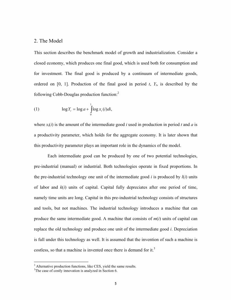
2. The Model

This section describes the benchmark model of growth and industrialization. Consider a

closed economy, which produces one final good, which is used both for consumption and

for investment. The final good is produced by a continuum of intermediate goods,

ordered on [0, 1]. Production of the final good in period t, Yt, is described by the

following Cobb-Douglas production function:2

(1) ,)(logloglog1

0∫+= diixaY tt

where xt(i) is the amount of the intermediate good i used in production in period t and a is

a productivity parameter, which holds for the aggregate economy. It is later shown that

this productivity parameter plays an important role in the dynamics of the model.

Each intermediate good can be produced by one of two potential technologies,

pre-industrial (manual) or industrial. Both technologies operate in fixed proportions. In

the pre-industrial technology one unit of the intermediate good i is produced by l(i) units

of labor and k(i) units of capital. Capital fully depreciates after one period of time,

namely time units are long. Capital in this pre-industrial technology consists of structures

and tools, but not machines. The industrial technology introduces a machine that can

produce the same intermediate good. A machine that consists of m(i) units of capital can

replace the old technology and produce one unit of the intermediate good i. Depreciation

is full under this technology as well. It is assumed that the invention of such a machine is

costless, so that a machine is invented once there is demand for it.3

2 Alternative production functions, like CES, yield the same results. 3The case of costly innovation is analyzed in Section 6.

5

We next add two assumptions on the function m, which lead to the result of long-

run growth. First, order the intermediate goods by increasing cost of machines, m(i), and

assume that:

(2) .)( 1 ∞→→iim

Namely, machines required to produce intermediate goods, which are close to 1, become

increasingly complicated and costly. In other words, some jobs, like a CEO, or an

engineer, are very hard to replace by a machine. It is also assumed that this complexity

does not make overall industrialization too expensive, namely it is assumed that the sum

of logarithms of machine costs over all potential machines is bounded:

(3) .log)(log1

0

∞<=∫ bdiim

The parameter b, which is finite, is therefore defined by equation (3). This second

assumption is necessary for long-run growth, as shown below.4 For the sake of

simplification it is assumed that the functions k, l, and m are all continuous.

We next describe individuals in the economy. Assume that it consists of a mass L

of identical individuals with infinite horizons. Each person supplies 1 unit of labor in

each period and has the following utility from consumption:

(4) .)1()log(

0∑∞

= +=

tt

tcU

ρ

The use of logarithmic utility is for simplification only and the results of the paper hold

for any utility function.

4 Actually, if a CES production function is used in (1), instead of Cobb-Douglas, (3) is not required if the elasticity of substitution is greater than 1.

6

3. Industrialization and Factor Prices

The main decision facing producers is choice of technology, namely whether to stick to

the old pre-industrial technology or to industrialize. The decision depends on factor

prices, since industrialization involves reduction of labor, but at the expense of

purchasing more capital. Producers of i adopt the new technology and industrialize in

period t if:

),()()( ilwikRimR ttt +≤

where wt is the wage rate and Rt is the gross rental rate of capital or the gross interest rate,

paid in period t on capital invested in period t – 1. Written differently, production of i is

industrialized if:

.)(

)()(

t

t

Rw

ilikim≤

−

Thus, the set of intermediate goods produced by machines in period t, namely the

industrial set It, is equal to:

(5) .)(

)()(:

≤−

=t

tt R

wil

ikimiI

Hence, the degree of industrialization depends crucially on the wage rate relative to the

rate of return. Higher wages create incentive to invent and use more technologies, as

these enable reduction of costly labor input. Lower wages deter industrialization, as

workers are inexpensive relative to costly machines.

In order to present the set of industrial intermediate goods It diagrammatically,

note that this set can also be described by:

(6) .)()()(:

+≤= ilRw

ikimiIt

tt

7

The industrialization of the economy is thus described in Figure 1. Clearly, as the ratio of

factor prices wt/Rt rises, the industrial set It increases. Note that if the factors’ price ratio

wt/Rt is very low, no intermediate good is industrialized, since m for all i, so that

the industrialization set is empty. This is the case of a pre-industrialized economy, like

the world prior to the industrial revolution. As is clear from this figure and from the

analysis above, the degree of industrialization depends on the factor prices, namely on the

prices of labor and capital. We next turn to describe how these prices are determined.

)()( iki >

[Insert Figure 1 here]

Perfect competition in the markets for intermediate goods leads to the following

profit maximization condition:

(7) .)()(

)(ix

Yix

Yip

t

t

t

tt =

∂∂

=

This describes the demand for the intermediate good. Its supply is perfectly elastic due to

fixed marginal productivity. Hence the price of each intermediate good is:

(8)

∉+∈

=+=.if)()(

if)()}()(),(min{)(

ttt

tttttt IiilwikR

IiimRilwikRimRip

Substituting (8) in (7) and then in (1) we get the following relationship between the wage

rate, the interest rate and the degree of industrialization:

(9) .log)]()(log[)](log[

)]}()(log[)],(min{log[1

0

adiilwikRdiimR

diilwikRimR

ctt I

ttI

t

ttt

=++=

=+

∫∫

∫

This equation defines the factor price frontier.

An alternative way to present equation (9) is to view the integral on the LHS as a

function of the two factor prices, namely:

8

(10) .)]}()(log[)],(min{log[),(1

0∫ += diiwliRkiRmRwH

It can be shown that H is concave and increasing in both w and R. From equation (9) it

follows that the factor price frontier is defined by:

(11) .log),( aRwH tt =

The factor price frontier can also be written as an explicit function: , where h

is defined by .

)( tt Rhw =

aRRhH log]),([ =

It is easy to show that h is decreasing and convex. We show in the next lemma

that the gross rate of interest is bounded from below on the factor price frontier.

Lemma 1: The factor price frontier satisfies: . Hence, as the wage rate w goes to

∞, the gross interest rate R goes to a / b.

baR /≥

Proof: In the Appendix.

Figure 2 describes the factor price frontier, )( tt Rhw = , based on the analysis

above. Figure 2 also describes how the factor price frontier determines the levels of

output and capital in the economy, as explained below.

[Insert Figure 2 here]

To see how to derive from the factor price frontier the capital-labor ratio and

output per worker, as shown in Figure 2, we analyze the equilibrium conditions in the

labor market and in the capital market. The labor market equilibrium condition is:

(12) .)()(

)()()( ∫∫ +

==ct

ct I tt

t

It di

ikRilwYil

diixilL

9

The capital market equilibrium condition is:

(13) .)()(

)()()(

)()()()( ∫∫∫∫ ++=+=

ctt

ctt I tt

t

I t

t

It

Itt di

ikRilwikY

diimRimY

diixikdiiximK

Lemma 2: The function H satisfies:

wI

HdiiRkiwl

ilc

=+∫ )()(

)( ,

and:

RII

HiRm

imdiiRkiwl

ikc

=++ ∫∫ )(

)()()(

)( .

Hence: .1=+ wR wHRH

Proof: In the Appendix.

From equation (12) and Lemma 2 we derive the following:

(14) ).,( ttwt RwHYL =

This condition determines the level of output Yt as a function of the factor prices. From

the capital market equilibrium condition (13) and Lemma 2 is:

(15) ).,( ttRtt RwHYK =

Hence, the capital labor ratio is described by: )(// twRtt RhHHLKk ′−=== . Namely,

the capital labor ratio is the slope of the factor price frontier. To graphically describe

output per worker, note that due to Lemma 2, total gross income is equal to gross output:

.)( tRtwttttt YHRHwYKRLw =+=+

Hence output per worker can also be described by Figure 2:

10

.tttt

ttt

t kRwL

KRw

LY

y +=+==

Figure 2 also describes the output-capital ratio, which we denote by qt:

.t

tt k

yq =

Clearly qt is increasing with Rt and converges to a/b as Rt goes down to a/b.

4. The Dynamics of Industrialization

The dynamic solution of the model follows the two standard conditions of a

representative agent economy. One is the first order condition of utility maximization and

the second is the goods market equilibrium. The utility maximization FOC is:

(16) .1

11

ρ+= ++ t

t

t Rc

c

The goods market equilibrium condition is:

(17) ).()()( 111 +++ ′+′−=−+=−= ttttttttttt RhRhRRhkkRwkyc

The dynamic Rational Expectations solution to these two dynamic equations, which

satisfies the No-Ponzi-Game condition, is a saddle path that converges to a steady state.

We next show that there are two dynamic cases.

In order to analyze the dynamics of this economy, where consumption can grow

forever, we define a new variable, the ratio between consumption and capital:

.t

tt k

cv =

Substituting in equations (16) and (17) we derive two dynamic equations of the system

with the variables vt and Rt. The equation that describes the dynamics of R is:

11

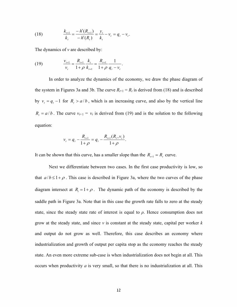
(18) .)()( 11

tttt

t

t

t

t

t vqvky

RhRh

kk

−=−=′−′−

= ++

The dynamics of v are described by:

(19) .111

1

1

11

tt

t

t

tt

t

t

vqR

kkR

vv

−+=

+= +

+

++

ρρ

In order to analyze the dynamics of the economy, we draw the phase diagram of

the system in Figures 3a and 3b. The curve Rt+1 = Rt is derived from (18) and is described

by for , which is an increasing curve, and also by the vertical line

. The curve v

1−= tt qv

ba /=

baRt />

Rt t+1 = vt is derived from (19) and is the solution to the following

equation:

.1

),(1

11

ρρ +−=

+−= ++ ttt

tt

ttvRR

qR

qv

It can be shown that this curve, has a smaller slope than the tt RR =+1 curve.

Next we differentiate between two cases. In the first case productivity is low, so

that ρ+≤1/ba . This case is described in Figure 3a, where the two curves of the phase

diagram intersect at ρ+=1tR . The dynamic path of the economy is described by the

saddle path in Figure 3a. Note that in this case the growth rate falls to zero at the steady

state, since the steady state rate of interest is equal to ρ. Hence consumption does not

grow at the steady state, and since v is constant at the steady state, capital per worker k

and output do not grow as well. Therefore, this case describes an economy where

industrialization and growth of output per capita stop as the economy reaches the steady

state. An even more extreme sub-case is when industrialization does not begin at all. This

occurs when productivity a is very small, so that there is no industrialization at all. This

12

happens if in Figure 1 the two curves do not intersect. In this case the economy remains

in a pre-industrialized equilibrium.

[Insert Figures 3a and 3b here]

The second case is when productivity a is sufficiently high, so that ρ+>1/ba .

This case is described in Figure 3b. Here the economy converges along the saddle path to

a steady state described by baR /* = and ρ

ρ+

=1

*bav . Therefore, the economy

experiences long-run growth. Formally, the rate of growth of consumption converges to

g, where:

(20) .01)1(

>−+

=ρb

ag

Since vt converges to a finite number and so does xt, it follows that both output and

capital grow permanently and that their long-run growth rates are equal to g as well.

Hence, this model of machines that replace workers can generate long-run growth. We

can therefore summarize the above discussion in the following Proposition.

Proposition 1: There is a unique equilibrium path. If a > b(1 + ρ) the economy grows

forever and the rate of growth converges to g. If a ≤ b(1 + ρ), growth peters out and the

economy converges to a steady state without growth.

This model therefore shows that the long-run rate of growth depends crucially on

the overall productivity of the economy a. A one-time shock to productivity can lead to

increased growth over a long period of time and even to permanent growth. To gain a

better understanding of this result we use the analysis of the aggregate production

13

function, which is done in the next proposition. This proposition also proves the

optimality of the competitive equilibrium.

Proposition 2: Let be the maximum amount of output that can be produced by L

workers and K

),( LKF t

t capital. Then: Y ),( LKF tt = . Namely, production is optimal in the market

economy. Also, the marginal productivities of labor and capital are equal to wt and Rt,

respectively. Furthermore, the intertemporal equilibrium is optimal as well.

Proof: In the Appendix.

Proposition 2 can help us better understand the strong dependency of dynamics on

productivity a. The marginal productivity of capital, when technology is endogenous, is

bounded from below by a/b. Hence, if this bound is sufficiently large, long-run growth

prevails. In this respect the model is very similar to the AK models of Jones and Manueli

(1990) and Rebelo (1991). But it also differs significantly from these AK models. First, it

has a micro-model of technology and innovation, which generates the AK relation.

Second, the mechanism through which the economy grows is very different. While in the

AK models growth is driven by the high marginal productivity of capital, in this model it

is driven by high wages. High productivity raises labor costs and increases the incentives

to use more machines. Once these additional machines are used, wages rise by more,

since intermediate goods cooperate in the production of the final good. That raises the

incentive to invest in more costly machines and put them into use. And so the process of

industrialization is rolling on, creating incentives for further industrialization at each step

on the way. This difference between the two models is not just in the description of the

14

mechanism of growth, but it has significant implication, like the effect of monopoly

power on growth, which is discussed in the next section.

5. Monopolies, Wages and Growth

In this section we deviate from perfect competition and examine what happens if

producers of intermediate goods have monopoly power. This can reflect social norms,

like Feudalism, or other causes. We assume that the monopoly power is exogenous and

examine how it affects growth. Intuitively, the effect of monopoly power on growth

should be negative, since monopoly power enables producers to reduce wages and that

reduces growth in our framework. The rest of the section formalizes this insight.

Assume that producers of intermediate goods have a monopoly power so that they

earn a profit, which equals a share z of revenues. Such profits arise is when there are N

producers of each intermediate good, who form an oligopoly. If they participate in a

Cournot competition and if N > 1, then in a symmetric equilibrium each producer earns a

profit, which is equal to a share z of revenues, where:

.122NN

z −=

If producers earn a profit of rate z, the price of each intermediate good is equal to:

(21)

∈−

∉−+

=.if

1)(

if1

)()(

)(

tt

ttt

t

IizimR

Iiz

ikRilw

ip

Combining (21) with equation (7) and substituting in equation (1) we get the following

factor price frontier:

15

(22) .log)1log()]}()(log[)],(min{log[1

0

azdiilwikRimR ttt =−−+∫

Hence, in a monopolistic economy the factor price frontier is affected not only by

productivity a, but by the degree of monopoly power z as well. As monopoly power

increases the factor price frontier shifts to the left. It is clear from (22) that as wages rise

to infinity, the gross rate of interest R converges to:

).1( zba

−

The solution of the rest of the model is the same as in Section 4, except that a/b is

replaced by a(1 – z)/b.5 Thus, the condition for long-run growth is more restrictive under

monopoly:

.1)1( ρ+>− zba

If this condition holds and the economy experiences long-run growth, its steady state

growth rate is:

.1)1()1(−

+−

=ρbzag

Hence, monopoly power impedes growth and it can even bar the economy from growing

and keep it stagnant. This result is opposite to that of AK models. The mechanism

through which the monopoly effect operates is by lowering wages, which is detrimental

to growth.6

5 Note that although agents are not identical under monopoly, as workers and producers earn different incomes, the dynamic equations of the model are the same. Since consumption dynamics are linear for each individual: ct+1 = ct Rt+1 (1+ρ)-1, they can be aggregated across individuals. The goods market equilibrium condition is also the same: kt+1 = yt – ct. 6 The effect of wages on growth is also studied recently by Saint-Paul (2005), but through its effect on consumption and demand.

16

6. Costly Innovations and the Effect of Scale

While section 5 examines the differences between this model and the AK literature, this

section compares this model with the other branch of endogenous growth models, based

on R&D. Similar to these models growth in this paper is also driven by new innovations.

But these models focus only on the innovation cost of new technologies, while this paper

focuses on the cost of the machines within which these new technologies are embodied.

So far the model has assumed for simplicity that the cost of innovation is zero. This

section discusses the case of positive innovation costs, so that a comparison with R&D

based growth models becomes more transparent.

Consider the model presented in Section 2 with the following extension. Inventing

a new machine is costly. The cost of innovation is assumed to be proportional to output

per capita:7

(23) .1

LY

dI tt

+=

Let us further assume that a patent on innovation lasts only one period and in next periods

the innovation becomes public knowledge. Hence, a machine i invented in period t-1

costs m(i) in future periods, but )()( izim + in first period of purchase, namely when

invested in period t-1. Due to competition among innovators the patent fee z(i) for an

invented machine is equal to:

(24) .)1()(

)(//

)()( 11

Lgidp

ipYLdY

ixI

izt

t

tt

t

t

t

+=== −−

The price of the good in first period of invention is equal to:

7 This is of course a simplifying assumption. Alternative assumptions on cost, like wages, yield similar results.

17

).()()( izRimRip ttt +=

Together with (24) this yields:

(25) ).()1(

)( imdRLg

dRiz

tt

t

−+=

Hence, a machine i is introduced in period t if:

(26) ).()()1(

)1()( il

Rw

ikdRLg

Lgim

t

t

tt

t +≤−+

+

Equation (26) shows that with costly innovations there is a scale effect, and a

larger scale L can speed innovations. But the scale effect in this model is diminishing

with scale, and as L becomes large enough it becomes negligible and the model

converges to the benchmark model. Thus, the scale effect, which is so troubling in the

original R&D growth models, as shown by Jones (1995a), is much reduced here. The

intuitive reason for that is straightforward. The cost of adopting an innovation is the sum

of the cost of innovation and the cost of the physical machine in which the innovation is

embodied. As the scale increases the cost of innovation per user falls, but the cost of the

machine remains unchanged. Hence, the benefit from scale is diminishing. Thus, scale

can help economic growth, but only to a limited and diminishing extent.

7. The Industrial Revolution

The next three sections turn to some empirical implications of the model presented in this

paper. This section examines how it can contribute to understanding the timing of the

industrial revolution. We know from various sources, like Maddison (1995), that

economic growth is a fairly recent phenomenon. It started somewhere in the beginning of

the 19th century and has been going steadily since then. It is also clear that growth is

18

inherently related to the process of industrialization. Hence, this model of growth through

industrialization seems suitable to study the industrial revolution. We should therefore

ask what, according to this model, can push the economy from a pre-industrial

equilibrium into industrialization.

Theoretically, the model offers two potential explanations, namely two exogenous

events that could have triggered the industrial revolution. One is a rise in productivity a.

Such a rise in productivity that takes the economy over the threshold of b(1 + ρ) can start

a process of long-run growth, as shown in Section 4. Thus, a rise in productivity could

have triggered the industrial revolution, by increasing the cost of labor and creating

incentives to use machines, which as a result are invented, produced and used all over the

world. The second potential explanation to the industrial revolution could be a reduction

in monopoly power. A stagnant economy can start industrialization and economic growth

by reducing its monopoly power, as shown in Section 5. The reduction of monopoly

power raises wages and creates incentives to industrialization and growth. A third

possible explanation could be an increase of scale, as in the R&D growth models and as

shown in Section 6 of this paper. We focus in this section on the two first potential

explanations, as they are more unique to this model.

What are the historical equivalents of an increase in productivity or of a reduction

in monopoly power prior to the industrial revolution? Two possible answers come to

mind. One is that the rise in productivity in Western Europe could have been the result of

the discovery of America. This contributed to sea faring, to agriculture, through discovery

of new plants and animals, and also by adding new territories, as described in Maddison

(2001, p. 18). This discovery raised incomes and as a result the cost of labor increased as

19

well. The rise in income after the discovery of America is documented in Maddison

(2001). Between 1500 and 1820 income per capita in Western Europe, North America

and Japan increased by more than 60%. This gives some indication to an increase in

productivity. Hence, the discovery of America, and the rise in productivity it created,

could be one potential trigger to the beginning of the industrial revolution.

The other historical development that could have triggered the industrial

revolution was the decline of Feudalism. This happened first in England following the

Cromwell Revolution, then in France during the Revolution, and in Germany later on.

During the 19th century all over Europe the old system of control by few over land and

production began crumbling down. Our model claims that these historical developments

could also trigger and enable the industrial revolution.

The scope of this paper is of course not sufficient to seriously assess these two

explanations to the beginning of the industrial revolution. It is possible that the two

historical developments together contributed to it. It is also possible that the two events

were not completely independent of one another, and the discovery of America

contributed to the decline of Feudalism. This should be kept in mind when we try to test

some of the ideas of this paper by looking at the historical data. Also, the relationships

between the discovery of America, the collapse of Feudalism and the industrial revolution

have been noted before.8 The specific contribution of this paper is twofold. The first is the

direction of causality from the two events to the industrial revolution, and the second is

pointing at the cost of labor as the main mechanism of effect.

8 One example that comes to mind is of course the Communist Manifesto by Marx and Engels (1998).

20

8. The Shares of Labor and Capital

The model of machines that replace workers in various stages of production yields some

very realistic results, as shown above. It can explain how output can grow at high rates

over a long period of time. It explains how the capital labor ratio grows with output. But

this model has one result which is in contrast with the empirical experience. According to

the benchmark model the share of capital in output, which is equal to Rt/qt, rises to 1,

while the share of labor in output falls gradually to zero. This has not happened in the last

two centuries of economic growth, during which the shares of labor and capital have been

quite stable at around 2/3 and 1/3 respectively. In this section we present an extension of

the model that avoids this unrealistic result of diminishing share of labor, but maintains

the other results of the model.

This section adds a second final good to the economy. This good is produced with

capital and labor, but is assumed to have no technical progress and there are no machines

that can help in its production. Many services fit this description, like education, arts and

literature, personal services, etc. We therefore assume that there are two goods in the

economy. One is a physical good that is produced as described in Section 2, and is used

for consumption and investment. The other good is services, which is used for

consumption only, and is produced by labor and capital in fixed proportions. One unit of

services is produced by 1 unit of labor and k* units of capital. Utility is derived from

consumption of the physical good c and consumption of the service good s:

(27) .)1(loglog

0∑∞

= ++

tt

tt scρα

It is further assumed that the size of the population is fixed and equal to 1.

21

Due to perfect competition in the labor market and to the linear technology of

production of services, the price of the service good is *kRw tt + . It follows that the

demand for the service good satisfies:

(28) .*kRw

cs

tt

tt +=

α

In other words, the share of services in total consumption expenditure is )1/( αα + . The

solution of the model leads to the following result:

Proposition 3: If productivity is sufficiently high, )1( ρ+> ba , there is sustainable long-

run growth, as in the benchmark model. Also, the share of labor does not diminish to zero

and it converges in the long-run to

.1 αρρ

αρ++

Proof: In the Appendix.

Note that if α = 2, so that the share of services in consumption is 2/3, and if ρ = 3,

which is reasonable for a period of 30 years, we get that the share of labor in income

converges to .6. Hence, the model, despite its great simplification, leads to results which

are close to the stylized facts.

This extension of the model, therefore, avoids the result that the share of labor in

income is diminishing to zero. It also has an additional interesting result. The share of

labor in services increases continually. This has two intuitive explanations. One is that

less and less workers are required in manufacturing, since they are replaced by machines.

Second, the price of the service good rises by less than income, as shown in Figure 2 and

22

as is clear intuitively. Hence, the demand for the service good increases and its

production increases with it.

9. Extensions

This section discusses briefly three additional implications of the approach presented in

the paper. First, it shows that the model can account not only for global growth, but also

for the great divergence between regions since the industrial revolution. Second, it shows

that energy prices can have a negative effect on the rate of economic growth. Note that

energy is strongly related to this model, since replacing workers by machines also

replaces human energy by thermal energy. Finally this section discusses the interpretation

of TFP growth along the growth path in this model.

9.1. Divergence between Regions

So far this model has been used to describe global economic growth, namely it implicitly

assumed that the closed economy is the world. Next we show that the model can be

applied to explain large and growing differences across countries. As shown in many

empirical studies, like Maddison (1995), Pritchett (1998), and Bourguignon and Morrison

(2002), gaps between regions in the world have been increasing significantly since the

beginning of the industrial revolution. This section shows how this model can account for

such findings.9

Consider a world with two countries, or regions, A and B. The two countries are

similar except in their basic productivity a, and it is assumed that aA > aB. Furthermore,

assume that:

9 Zeira (1998) already uses a similar model to explain differences across countries. This section further strengthens this result.

23

(29) .1ba

ba BA >+> ρ

Assume also that there is full capital mobility in the world. For simplicity assume that the

intermediate goods are not tradable. The equilibrium in this economy is easy to solve.

Clearly the gross interest rate must satisfy: baR At >

1) 1 −−ρ

. Hence, economy A grows at a

positive rate, which is higher than . Economy B is stagnant and gets

stuck at a fixed level of wages and output per capita.

1(1 +−baA

10

This model can therefore account for very different growth performance in

different regions in the world, due to disparities in basic productivity. It is interesting to

examine the data presented by Maddison (2001) with respect to two main regions. Region

A is Western Europe, Western Offshoots and Japan. Region B is the rest of the world. In

1500 GDP per capita in A was 704, while GDP per capita in B was 535. Until 1820 GDP

per capita in A rose to 1,130, more than 60%, while GDP per capita in B rose only to 573,

a rise of 7%. This shows that at the outset of the industrial revolution the productivity

difference between regions was already significant.

Finally, the model can be applied in a similar way to differences in cost of

machines, in addition to differences in productivity. A country that faces a high cost of

machines, due to import costs, has a higher b and as a result growth slows down and may

even stagnate completely. This result of the model is related to the empirical finding of

Barro (1991) and other recent cross-country studies, who find that high costs of

investment goods have a strong negative effect on growth.

10 This equilibrium has one aspect which is not realistic, namely that consumption in both A and B grows at the same rate. This means that consumption in the stagnant economy has very low levels in period 0. This result is due to the Ramsey framework and to having the same interest rate in both economies. One way to avoid this type of result is to assume instead an overlapping generations economy with utility from bequests, and with minimum subsistence consumption.

24

9.2. Energy and Growth

Actually the machines that replace humans in various tasks and jobs require energy to

operate. In a way machines that replace workers also replace the source of energy, from

human energy to fossil energy, either coal or oil. Thus, if we want to model the process of

replacing workers by machines more realistically, we should add the energy requirements

of machines as well. Next we extend the model in this direction in a very simplified way.

Assume that when an intermediate good i is produced by machines it requires a machine

of size m(i) and an input of energy of size e(i). Assume that the price of energy is q, and

that it is fixed over time. Clearly, the condition for industrialization is similar to the

benchmark model:

(30) ).()()()( ilwikRiqeimR ttt +≤+

The condition that determines the factor price frontier is:

(31) .log)]}()(log[)],()(min{log[1

0

adiilwikRiqeimR ttt =++∫

It can be shown that the equilibrium is similar to the industrial growth equilibrium

described above in Section 5. But the long run growth in this case depends crucially on

the price of energy. If the price rises during the period of industrialization it can hold it

down and even stop it. Thus according to this model the growth process is inherently

bounded by the supply of energy on our planet. Of course, we can assume that the stock

of energy on our planet is large enough, and that even when it is depleted we will be able

to find other ways of harnessing solar energy to our use. But this brief analysis

demonstrates that the price of energy is crucial for the process of industrialization and

economic growth.

25

9.3. TFP Growth

Economic growth is accompanied with the growth of the Solow residual, also called total

factor productivity. In this paper it is hard to distinguish between capital accumulation

and total factor productivity, since technologies are embodied in machines, in capital

goods. We next examine directly total factor productivity, which is measured as follows:

.log)1(log)]1log()1(log[

loglogloglogloglog

−++−−−−=

=

−

−=−−

RwsRssss

wYs

sRYs

sYLsKsY

KKKKK

LL

KKLK

Note that the first item on the RHS is the entropy of sK and is thus quite stable. So is the

interest rate in our model, namely log R. Hence, most of the changes in TFP are driven by

changes in wages. Hence, TFP growth might measure not exogenous productivity, but

rather rising wages. As shown in this model, these wages are also intricately related to the

process of growth, industrialization and technical progress, but the causalities might be

very different.

10. Summary

This paper presents a model of industrialization, describing it as a process of inventing

new machines that replace workers in a growing set of tasks. In this process the wage rate

plays a critical role. Wages serve as an incentive for adopting new technologies. But

wages are also affected by adoption of technologies, since performance of some tasks by

machines raises wages of workers, who perform the remaining tasks, due to higher

marginal productivity. This feedback between wages and technology is the main

mechanism that drives the results of this paper. It explains how the growth process can

26

continue for long periods, it explains how growth is so sensitive to productivity, and it

also explains why monopoly deters growth.

Finally, we should briefly discuss the type of innovations in this paper, namely

machines that replace human labor. Although this is a specific type of innovation, it can

be shown to be quite common. Even an innovation that replaces a machine by a better

one, also enables the workers operating it to produce more, namely to use less labor in

production. Furthermore, even innovations of new consumption goods tend to replace

labor this way or the other. A dishwasher, TV dinner, radio, cinema, all replace labor,

either at home, or in other locations. We do not have to go back to the time of the

Ludites, to realize that new machines that replace human labor have had a central role in

economic growth since the industrial revolution. This paper shows that embodying this

insight into growth theory can help us significantly in understanding the growth process.

27

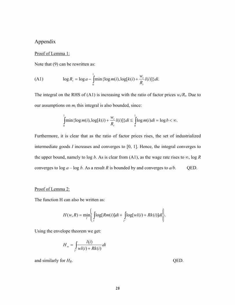
Appendix

Proof of Lemma 1:

Note that (9) can be rewritten as:

(A1) .)]}()(log[),(min{logloglog1

0∫ +−= diil

Rw

ikimaRt

tt

The integral on the RHS of (A1) is increasing with the ratio of factor prices wt/Rt. Due to

our assumptions on mi this integral is also bounded, since:

.log)(log)]}()(log[),(min{log1

0

1

0

∞<=≤+ ∫∫ bdiimdiilRw

ikimt

t

Furthermore, it is clear that as the ratio of factor prices rises, the set of industrialized

intermediate goods I increases and converges to [0, 1]. Hence, the integral converges to

the upper bound, namely to log b. As is clear from (A1), as the wage rate rises to ∞, log R

converges to log a – log b. As a result R is bounded by and converges to a/b. QED.

Proof of Lemma 2:

The function H can also be written as:

.)]()(log[)](log[min),(

++= ∫∫cII

IdiiRkiwldiiRmRwH

Using the envelope theorem we get:

∫ +=

cIw di

iRkiwlilH

)()()(

and similarly for HR. QED.

28

Proof of Proposition 2:

Maximum output Y is defined by: ),( LKF=

(A2) .)()(,)()()()(:)(loglogmaxlog1

0)(,

==++= ∫ ∫ ∫∫I II

ixIcc

LdiixilKdiixikdiiximdiixaY

The maximization of (A2), using two shadow prices, q1 and q2 for the two constraints

respectively, yields the following first order conditions:

(A3) ),()(

11 imq

ix=

if i , and I∈

(A4) ),()()(

121 ilqikq

ix+=

if i , and I∉

(A5) ),()()( 211 ilqikqimq +=

at the border points between I and Ic. Define YqR 1= and Yqw 2= . By substituting (A2),

(A3) and (A4) into the production function (1) we get:

.log),( aRwH =

Hence, the optimal allocation of labor and capital between the intermediate goods is the

equilibrium allocation and output is optimal.

Note that:

.1log1 Y

RqY

MPKdK

Yd===

Hence the marginal productivity of capital is equal to R and similarly the marginal

productivity of labor is equal to w.

A central planner maximizes output in each period and intertemporally maximizes:

29

(A6) .)1(

)log()1(

log0

1

0∑∑∞

=

+∞

= +−

=+ t

ttt

tt

t kycρρ

It can be shown that the first order conditions of this maximization are equal to the

dynamic conditions of the competitive equilibrium. Hence, the competitive equilibrium is

optimal. QED.

Proof of Proposition 3:

Note first that from utility maximization we get the first order condition:

,1

11

ρ+= ++ t

t

t Rc

c

so that the long run growth of consumption is:

.011

/>−

+=

ρbag

Denote by K the amount of capital in production of the physical good. Then the rate of

growth of K is:

.**1

t

t

t

tt

t

ttt

t

t

Kks

Kc

qK

kscYK

K−−=

−−=+

Since qt converges to a/b and since s is bounded by 1, it follows that the rate of growth of

capital must converge to that of consumption. Hence the ratio between consumption of

the physical good and capital in its production converges to:

.)1( ρ

ρ+ba

Second, note that the amount of labor in production of the physical good is no longer

equal to the overall supply of labor. Due to (28) this amount of labor is equal to:

30

(A7) .*

11kRw

csL

tt

ttt +

−=−=α

From equation (A7) and from Figure 2 we get:

./*

1*)(

11tttt

t

t

t

tttt

ttt kkRRq

LKc

kRRqkc

sL+−

−=+−

−=−= αα

Since c/K converges to a finite number, since q – R converges to zero, and so is k*/k, it

therefore follows that Lt converges to zero as the economy grows. Hence, the share of

labor in production of the physical good converges to zero, while the share of labor in

production of services increases continuously to 1. The amount of services s converges to

1 as well.

We next calculate the ratio between labor income and capital income:

.1*

*/* ρ

αραα+

=→+−

=+ ∞→ sRK

ckRsKRkRsc

kRsKRw

ttttt

ttt

tttt

t

Hence the share of labor in total income converges to:

.1 αρρ

αρ++

The share of labor therefore does not diminish to zero. QED.

31

References

Aghion, Philippe, and Howitt, Peter. “A Model of Growth through Creative Destruction,” Econometrica, Vol. 60 (2), March 1992, p. 323-351.

Aghion, Philippe, and Howitt, Peter. Endogenous Growth Theory. Cambridge, MA: MIT

Press, 1998. Barro, Robert j., “Economic Growth in a Cross Section of Countries,” Quarterly Journal

of Economics, 106 (1991), 407-443. Barro, Robert J., and Sala-i-Martin, Xavier. Economic Growth. New York: McGraw Hill,

1995. Beaudry, Paul, and Collard, Fabrice. “Why Has the Employment-Productivity Tradeoff

Among Industrialized Countries Been So Strong?” NBER Working Paper No. 8754, 2002.

Bourguignon, François, and Morrison, Christian, “Inequality Among World Citizens:

1820-1992,” American Economic Review, Vol. 92, Sep. 2002, p. 727-744. Champernowne, David, “A Dynamic Growth Model Involving a Production Function,” in

F.A. Lutz and D.C. Hague, eds., The Theory of Capital (New York: Macmillan, 1963).

De Long, Bradford J., “Productivity and Machinery Investment: A Long-Run Look,

1870-1980,” Journal of Economic History, LIII (1992). Grossman, Gene M. and Helpman, Elhanan. Innovation and Growth in the Global

Economy. Cambridge, MA: MIT Press, 1991. Habbakuk, H. J. American and British Technology in the Nineteenth Century. Cambridge:

Cambridge University Press, 1962. Jones, Charles I. “Time Series Tests of Endogenous Growth Models,” Quarterly Journal

of Economics, Vol. 110 (2), May 1995 (a), p. 495-525. Jones, Charles I. “R & D-Based Models of Economic Growth,” Journal of Political

Economy, Vol. 103, August 1995 (b), p. 759-784. Jones, Charles I. and Williams, John C. “Too Much of a Good Thing? The Economics of

Investment in R&D,” Journal of Economic Growth, Vol. 5, March 2000, p. 65-85. Jones, Larry, and Manuelli, Rodolfo. “A Convex Model of Equilibrium Growth: Theory

and Implications,” Journal of Political Economy, Vol. 98, 1990, p. 1008-1038.

32

Maddison, Angus. Monitoring the World Economy 1820-1992. Paris, France: OECD, 1995.

Maddison, Angus. The World Economy: A Millenial Perspective. Paris, France: OECD,

2001. Marx, Karl, and Engels, Frederick. The Communist Manifesto. London: Verso, 1998. Pritchett, Lant. “Divergence, Big Time,” Journal of Economic Perspectives, Vol. 11,

Summer 1997, p. 3-17. Rebelo, Sergio. “Long Run Policy Analysis and Long Run Growth,” Journal of Political

Economy, Vol. 99, June 1991, p. 500-521. Romer, Paul M. “Endogenous Technical Change,” Journal of Political Economy, Vol. 98,

October 1990, p. S71-S102. Saint-Paul, Gilles. “Distribution and Growth in an Economy with Limited Needs,”

Economic Journal, forthcoming, 2005. Segestrom, Paul S., Anant T.C.A. and Dinopoulos, Elias. “A Schumpeterian Model of the

Product Life Cycle,” The American Economic Review, Vol. 80 (5), December 1990, p. 1077-1091.

Solow, Robert M., “A Contribution to the Theory of Economic Growth,” Quarterly

Journal of Economics, 71 (1956), 65-94. Solow, Robert M., “Technical Change and the Aggregate Production Function,” Review

of Economics and Statistics, 39 (1957), 312-320. Solow, Robert M., “Investment and Technical Progress,” in Kenneth J. Arrow, Samuel

Karlin and P. Suppes, eds., Mathematical Methods in the Social Sciences (Stanford: Stanford University Press, 1960).

Zeira, Joseph, “Workers, Machines and Economic Growth,” Quarterly Journal

of Economics, 113 (1998), 1091-1113. Zuleta, Hernando, “Why Factor Income Shares Seem to be Constant?” mimeo,

2003.

33

Figures

m(i)

k(i)+l(i)wt/Rt

i

1 It

Figure 1

34

w

yt

wt

h

R

a/b qt Rt

Figure 2

35

vt

Rt+1=Rt

vt+1=vt

a/b-1

Rt

a/b 1+ρ

Figure 3a

36

vt

Rt+1=Rt

vt+1=vt

a/b-1

v*

Rt

a/b

Figure 3b

37