


Machine Learning Methods: Applications in Biology and ...
73
Machine Learning Methods: Applications in Biology and Computer Vision Mario Banuelos, California State University, Fresno mbanuelos22 www.mbgmath.com [email protected]
Transcript of Machine Learning Methods: Applications in Biology and ...
Machine Learning Methods:Applications in Biology and ComputerVisionMario Banuelos, California State University, Fresno7 mbanuelos22 � www.mbgmath.com R [email protected]

Outline
1 Introduction & Background
2 Neural Networks and Computer Vision
3 Detecting Genomic Variation
4 Conclusions
M.Banuelos (Fresno State) [email protected] February 18, 2019
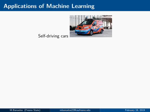
Applications of Machine Learning
Self-driving cars
Voice Assistants
Object Classification/Detection
M.Banuelos (Fresno State) [email protected] February 18, 2019
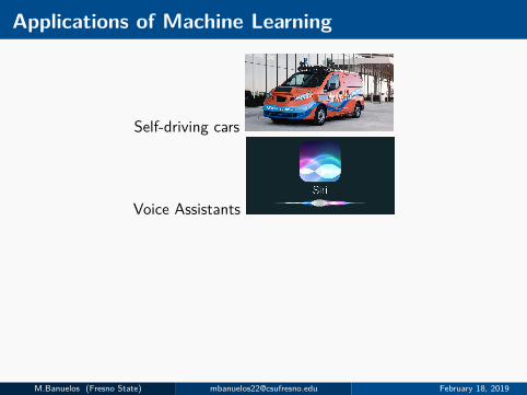
Applications of Machine Learning
Self-driving cars
Voice Assistants
Object Classification/Detection
M.Banuelos (Fresno State) [email protected] February 18, 2019
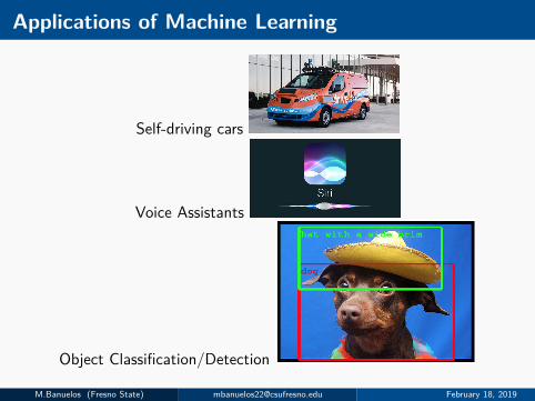
Applications of Machine Learning
Self-driving cars
Voice Assistants
Object Classification/Detection
M.Banuelos (Fresno State) [email protected] February 18, 2019
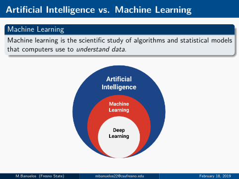
Artificial Intelligence vs. Machine Learning
Machine LearningMachine learning is the scientific study of algorithms and statistical modelsthat computers use to understand data.
M.Banuelos (Fresno State) [email protected] February 18, 2019
Artificial Intelligence vs. Machine Learning
Machine LearningMachine learning is the scientific study of algorithms and statistical modelsthat computers use to understand data.
M.Banuelos (Fresno State) [email protected] February 18, 2019
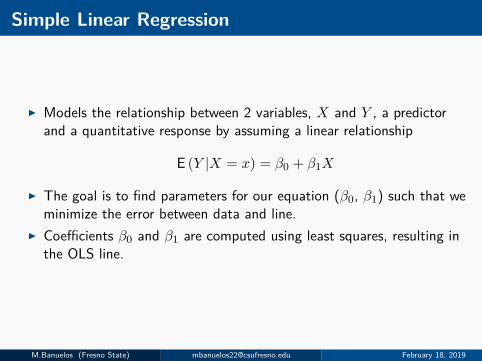
Simple Linear Regression
I Models the relationship between 2 variables, X and Y , a predictorand a quantitative response by assuming a linear relationship
E (Y |X = x) = β0 + β1X
I The goal is to find parameters for our equation (β0, β1) such that weminimize the error between data and line.
I Coefficients β0 and β1 are computed using least squares, resulting inthe OLS line.
M.Banuelos (Fresno State) [email protected] February 18, 2019
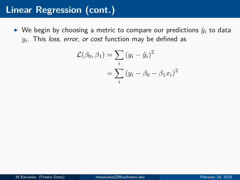
Linear Regression (cont.)
I We begin by choosing a metric to compare our predictions yi to datayi. This loss, error, or cost function may be defined as
L(β0, β1) =∑i
(yi − yi)2
=∑i
(yi − β0 − β1xi)2
I Then we find the βs, by solving
∂L(β0, β1)β0
= −2n∑i=1
(yi − β0 − β1xi) = 0
∂L(β0, β1)β1
= −2n∑i=1
xi(yi − β0 − β1xi) = 0.
M.Banuelos (Fresno State) [email protected] February 18, 2019
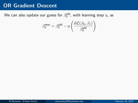
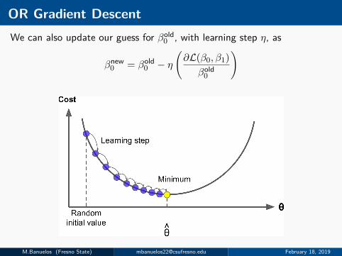
OR Gradient DescentWe can also update our guess for βold
0 , with learning step η, as
βnew0 = βold
0 − η(∂L(β0, β1)
βold0
)
M.Banuelos (Fresno State) [email protected] February 18, 2019
OR Gradient DescentWe can also update our guess for βold
0 , with learning step η, as
βnew0 = βold
0 − η(∂L(β0, β1)
βold0
)
M.Banuelos (Fresno State) [email protected] February 18, 2019
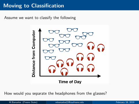
Moving to Classification
Assume we want to classify the following
How would you separate the headphones from the glasses?
M.Banuelos (Fresno State) [email protected] February 18, 2019
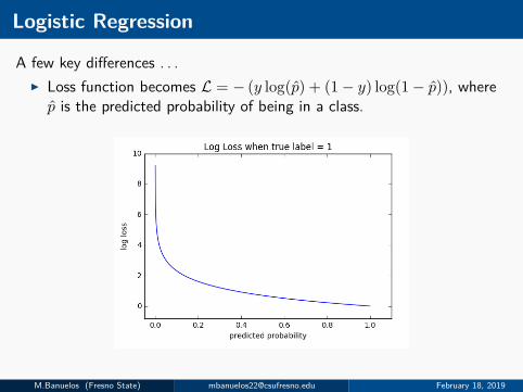
Logistic Regression
A few key differences . . .I Loss function becomes L = − (y log(p) + (1− y) log(1− p)), wherep is the predicted probability of being in a class.
M.Banuelos (Fresno State) [email protected] February 18, 2019
Logistic Regression
A few key differences . . .I Loss function becomes L = − (y log(p) + (1− y) log(1− p)), wherep is the predicted probability of being in a class.
M.Banuelos (Fresno State) [email protected] February 18, 2019

Logistic Regression
A few key differences . . .
We use log(
p1−p
)= β0 + β1X where p is referred to as the probability
that y = 1.
M.Banuelos (Fresno State) [email protected] February 18, 2019
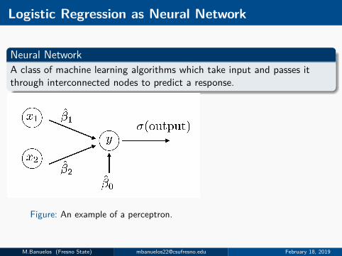
Logistic Regression as Neural Network
Neural NetworkA class of machine learning algorithms which take input and passes itthrough interconnected nodes to predict a response.
Figure: An example of a perceptron.
The Sigmoid Function
σ(x) = 1(1 + e−x)
M.Banuelos (Fresno State) [email protected] February 18, 2019
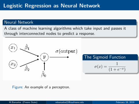
Logistic Regression as Neural Network
Neural NetworkA class of machine learning algorithms which take input and passes itthrough interconnected nodes to predict a response.
Figure: An example of a perceptron.
The Sigmoid Function
σ(x) = 1(1 + e−x)
M.Banuelos (Fresno State) [email protected] February 18, 2019
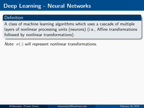
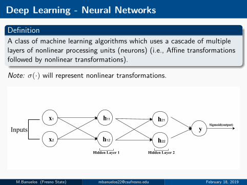
Deep Learning - Neural Networks
DefinitionA class of machine learning algorithms which uses a cascade of multiplelayers of nonlinear processing units (neurons) (i.e., Affine transformationsfollowed by nonlinear transformations).
Note: σ(·) will represent nonlinear transformations.
x1 h11
Inputsx2 h12
ySigmoid(output)
Hidden Layer 1
h21
h22
Hidden Layer 2
M.Banuelos (Fresno State) [email protected] February 18, 2019
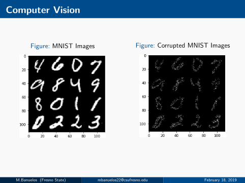
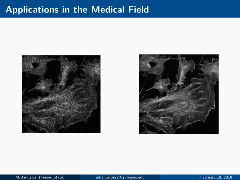
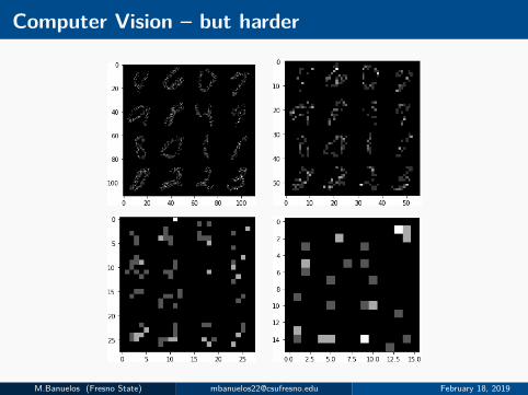
Computer Vision
Figure: MNIST Images Figure: Corrupted MNIST Images
M.Banuelos (Fresno State) [email protected] February 18, 2019
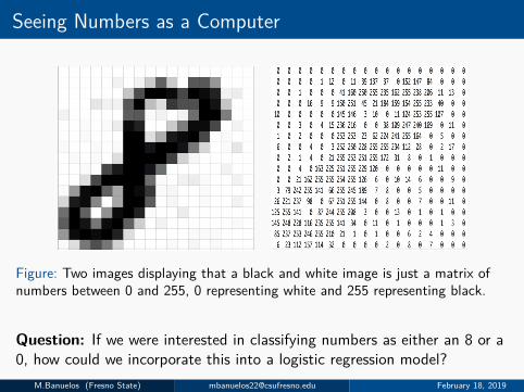
Seeing Numbers as a Computer
Figure: Two images displaying that a black and white image is just a matrix ofnumbers between 0 and 255, 0 representing white and 255 representing black.
Question: If we were interested in classifying numbers as either an 8 or a0, how could we incorporate this into a logistic regression model?
M.Banuelos (Fresno State) [email protected] February 18, 2019
Decision Boundaries are often Nonlinear
I Logistic regression will perform worse than a neural network with only1 hidden layer
I These tools are generalizable to natural language processing, biology,societal applications, and many more fields.
I But . . . more mathematicians are needed to design studies andinterpret the results.
M.Banuelos (Fresno State) [email protected] February 18, 2019
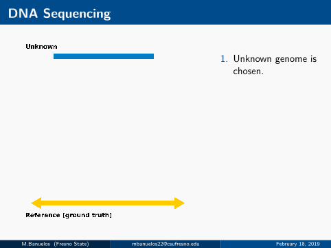
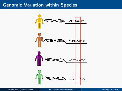
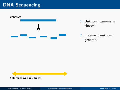
DNA Sequencing
1. Unknown genome ischosen.
2. Fragment unknowngenome.
3. Ends of fragments aresequenced.
4. Ends aligned toreference genome.
M.Banuelos (Fresno State) [email protected] February 18, 2019
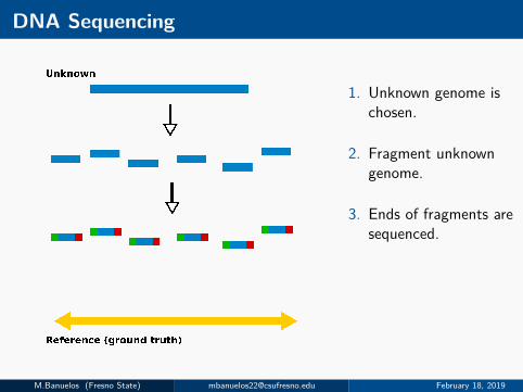
DNA Sequencing
1. Unknown genome ischosen.
2. Fragment unknowngenome.
3. Ends of fragments aresequenced.
4. Ends aligned toreference genome.
M.Banuelos (Fresno State) [email protected] February 18, 2019
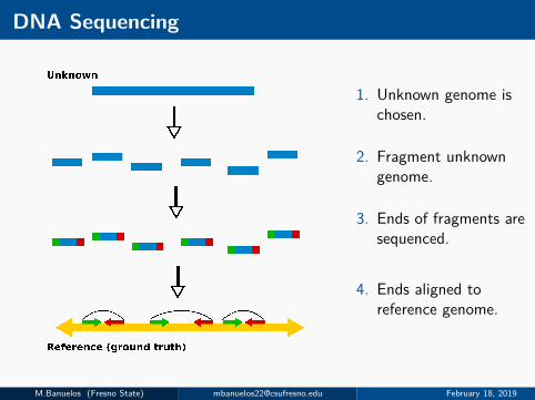
DNA Sequencing
1. Unknown genome ischosen.
2. Fragment unknowngenome.
3. Ends of fragments aresequenced.
4. Ends aligned toreference genome.
M.Banuelos (Fresno State) [email protected] February 18, 2019
DNA Sequencing
1. Unknown genome ischosen.
2. Fragment unknowngenome.
3. Ends of fragments aresequenced.
4. Ends aligned toreference genome.
M.Banuelos (Fresno State) [email protected] February 18, 2019
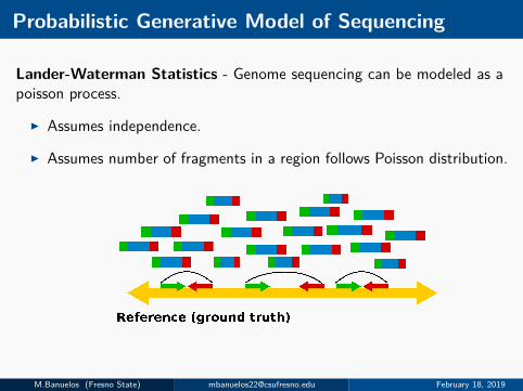
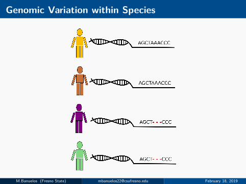
Probabilistic Generative Model of Sequencing
Lander-Waterman Statistics - Genome sequencing can be modeled as apoisson process.
I Assumes independence.
I Assumes number of fragments in a region follows Poisson distribution.
M.Banuelos (Fresno State) [email protected] February 18, 2019
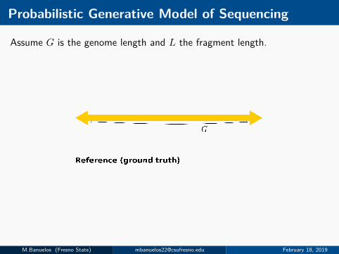
Probabilistic Generative Model of Sequencing
Assume G is the genome length and L the fragment length.
M.Banuelos (Fresno State) [email protected] February 18, 2019
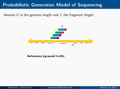
Probabilistic Generative Model of Sequencing
Assume G is the genome length and L the fragment length.
M.Banuelos (Fresno State) [email protected] February 18, 2019
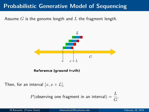
Probabilistic Generative Model of Sequencing
Assume G is the genome length and L the fragment length.
Then, for an interval [x, x+ L],
P (observing one fragment in an interval) = L
G.
M.Banuelos (Fresno State) [email protected] February 18, 2019
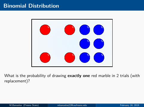
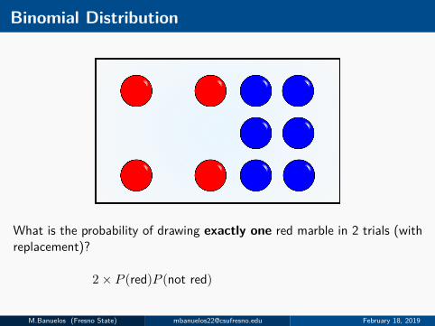
Binomial Distribution
What is the probability of drawing exactly one red marble in 2 trials (withreplacement)?
M.Banuelos (Fresno State) [email protected] February 18, 2019
Binomial Distribution
What is the probability of drawing exactly one red marble in 2 trials (withreplacement)?
2× P (red)P (not red)
M.Banuelos (Fresno State) [email protected] February 18, 2019

Binomial Distribution
What is the probability of drawing exactly one red marble in 2 trials (withreplacement)?
2× P (red)P (not red) = 2× (0.4)(0.6) = 0.48
.M.Banuelos (Fresno State) [email protected] February 18, 2019
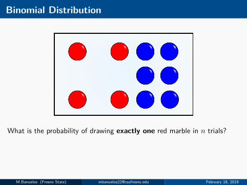
Binomial Distribution
What is the probability of drawing exactly one red marble in n trials?
M.Banuelos (Fresno State) [email protected] February 18, 2019
Binomial Distribution
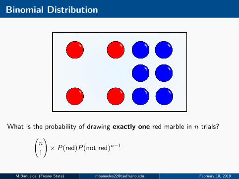
What is the probability of drawing exactly one red marble in n trials?(n
1
)× P (red)P (not red)n−1
M.Banuelos (Fresno State) [email protected] February 18, 2019

Binomial Distribution
What is the probability of drawing exactly one red marble in n trials?(n
1
)× P (red)P (not red)n−1 = n× (0.4)(0.6)n−1
.
M.Banuelos (Fresno State) [email protected] February 18, 2019
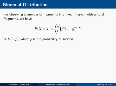
Binomial Distribution
For observing k number of fragments in a fixed interval, with n totalfragments, we have
P (X = k) =(n
k
)pk(1− p)n−k,
or B(n, p), where p is the probability of success.
M.Banuelos (Fresno State) [email protected] February 18, 2019
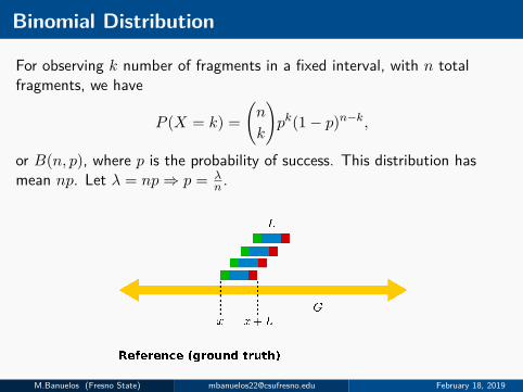
Binomial Distribution
For observing k number of fragments in a fixed interval, with n totalfragments, we have
P (X = k) =(n
k
)pk(1− p)n−k,
or B(n, p), where p is the probability of success. This distribution hasmean np. Let λ = np⇒ p = λ
n .
M.Banuelos (Fresno State) [email protected] February 18, 2019
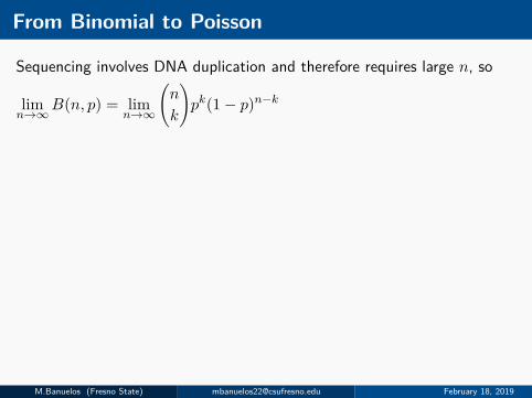
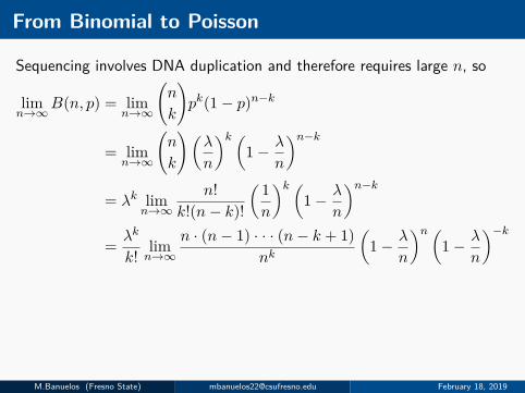
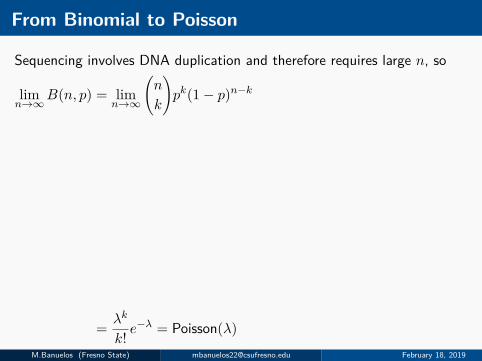
From Binomial to Poisson
Sequencing involves DNA duplication and therefore requires large n, so
limn→∞
B(n, p) = limn→∞
(n
k
)pk(1− p)n−k
= limn→∞
(n
k
)(λ
n
)k (1− λ
n
)n−k= λk lim
n→∞n!
k!(n− k)!
( 1n
)k (1− λ
n
)n−k= λk
k! limn→∞
n · (n− 1) · · · (n− k + 1)nk
(1− λ
n
)n (1− λ
n
)−k= λk
k! limn→∞
n · (n− 1) · · · (n− k + 1)nk︸ ︷︷ ︸→1
(1− λ
n
)n︸ ︷︷ ︸→e−λ
(1− λ
n
)−k︸ ︷︷ ︸
→1
= λk
k! e−λ = Poisson(λ)
M.Banuelos (Fresno State) [email protected] February 18, 2019
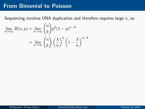
From Binomial to Poisson
Sequencing involves DNA duplication and therefore requires large n, so
limn→∞
B(n, p) = limn→∞
(n
k
)pk(1− p)n−k
= limn→∞
(n
k
)(λ
n
)k (1− λ
n
)n−k
= λk limn→∞
n!k!(n− k)!
( 1n
)k (1− λ
n
)n−k= λk
k! limn→∞
n · (n− 1) · · · (n− k + 1)nk
(1− λ
n
)n (1− λ
n
)−k= λk
k! limn→∞
n · (n− 1) · · · (n− k + 1)nk︸ ︷︷ ︸→1
(1− λ
n
)n︸ ︷︷ ︸→e−λ
(1− λ
n
)−k︸ ︷︷ ︸
→1
= λk
k! e−λ = Poisson(λ)
M.Banuelos (Fresno State) [email protected] February 18, 2019
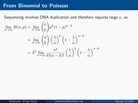
From Binomial to Poisson
Sequencing involves DNA duplication and therefore requires large n, so
limn→∞
B(n, p) = limn→∞
(n
k
)pk(1− p)n−k
= limn→∞
(n
k
)(λ
n
)k (1− λ
n
)n−k= λk lim
n→∞n!
k!(n− k)!
( 1n
)k (1− λ
n
)n−k
= λk
k! limn→∞
n · (n− 1) · · · (n− k + 1)nk
(1− λ
n
)n (1− λ
n
)−k= λk
k! limn→∞
n · (n− 1) · · · (n− k + 1)nk︸ ︷︷ ︸→1
(1− λ
n
)n︸ ︷︷ ︸→e−λ
(1− λ
n
)−k︸ ︷︷ ︸
→1
= λk
k! e−λ = Poisson(λ)
M.Banuelos (Fresno State) [email protected] February 18, 2019
From Binomial to Poisson
Sequencing involves DNA duplication and therefore requires large n, so
limn→∞
B(n, p) = limn→∞
(n
k
)pk(1− p)n−k
= limn→∞
(n
k
)(λ
n
)k (1− λ
n
)n−k= λk lim
n→∞n!
k!(n− k)!
( 1n
)k (1− λ
n
)n−k= λk
k! limn→∞
n · (n− 1) · · · (n− k + 1)nk
(1− λ
n
)n (1− λ
n
)−k
= λk
k! limn→∞
n · (n− 1) · · · (n− k + 1)nk︸ ︷︷ ︸→1
(1− λ
n
)n︸ ︷︷ ︸→e−λ
(1− λ
n
)−k︸ ︷︷ ︸
→1
= λk
k! e−λ = Poisson(λ)
M.Banuelos (Fresno State) [email protected] February 18, 2019

From Binomial to Poisson
Sequencing involves DNA duplication and therefore requires large n, so
limn→∞
B(n, p) = limn→∞
(n
k
)pk(1− p)n−k
= limn→∞
(n
k
)(λ
n
)k (1− λ
n
)n−k= λk lim
n→∞n!
k!(n− k)!
( 1n
)k (1− λ
n
)n−k= λk
k! limn→∞
n · (n− 1) · · · (n− k + 1)nk
(1− λ
n
)n (1− λ
n
)−k= λk
k! limn→∞
n · (n− 1) · · · (n− k + 1)nk︸ ︷︷ ︸→1
(1− λ
n
)n︸ ︷︷ ︸→e−λ
(1− λ
n
)−k︸ ︷︷ ︸
→1
= λk
k! e−λ = Poisson(λ)
M.Banuelos (Fresno State) [email protected] February 18, 2019
From Binomial to Poisson
Sequencing involves DNA duplication and therefore requires large n, so
limn→∞
B(n, p) = limn→∞
(n
k
)pk(1− p)n−k
= limn→∞
(n
k
)(λ
n
)k (1− λ
n
)n−k= λk lim
n→∞n!
k!(n− k)!
( 1n
)k (1− λ
n
)n−k= λk
k! limn→∞
n · (n− 1) · · · (n− k + 1)nk
(1− λ
n
)n (1− λ
n
)−k= λk
k! limn→∞
n · (n− 1) · · · (n− k + 1)nk︸ ︷︷ ︸→1
(1− λ
n
)n︸ ︷︷ ︸→e−λ
(1− λ
n
)−k︸ ︷︷ ︸
→1
= λk
k! e−λ = Poisson(λ)
M.Banuelos (Fresno State) [email protected] February 18, 2019
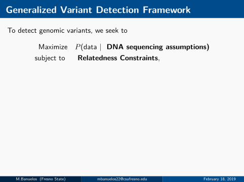
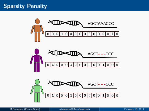
Generalized Variant Detection Framework
To detect genomic variants, we seek to
Maximize P (data | DNA sequencing assumptions)subject to Relatedness Constraints,
M.Banuelos (Fresno State) [email protected] February 18, 2019
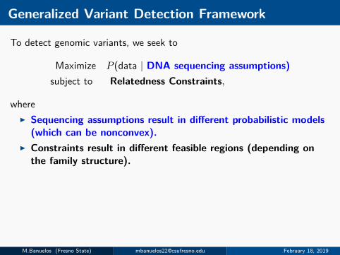
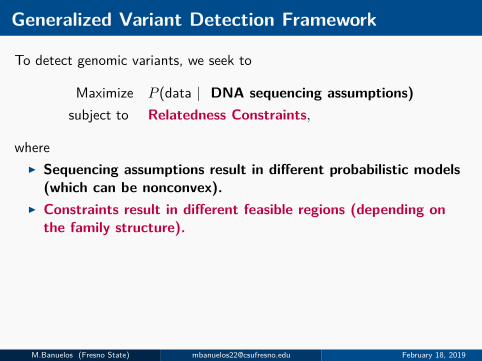
Generalized Variant Detection Framework
To detect genomic variants, we seek to
Maximize P (data | DNA sequencing assumptions)subject to Relatedness Constraints,
whereI Sequencing assumptions result in different probabilistic models
(which can be nonconvex).I Constraints result in different feasible regions (depending on
the family structure).
M.Banuelos (Fresno State) [email protected] February 18, 2019
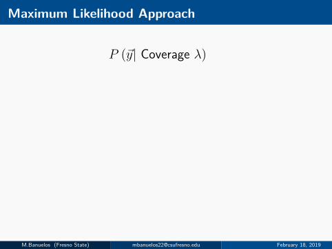
Maximum Likelihood Approach
P (~y| Coverage λ)
M.Banuelos (Fresno State) [email protected] February 18, 2019
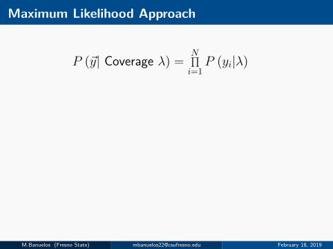
Maximum Likelihood Approach
P (~y| Coverage λ) =N∏i=1
P (yi|λ)
M.Banuelos (Fresno State) [email protected] February 18, 2019

Maximum Likelihood Approach
P (~y| Coverage λ) =N∏i=1
P (yi|λ)
Real SV Error
M.Banuelos (Fresno State) [email protected] February 18, 2019
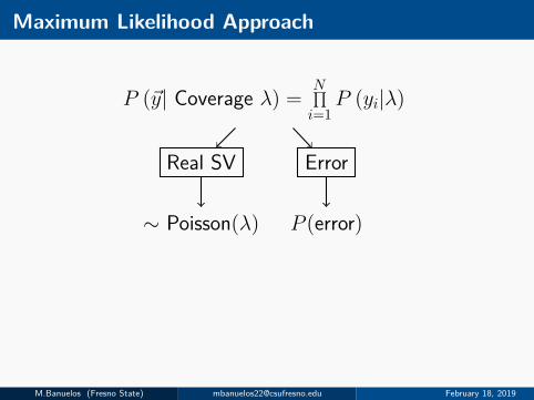
Maximum Likelihood Approach
P (~y| Coverage λ) =N∏i=1
P (yi|λ)
Real SV Error
∼ Poisson(λ) P (error)
M.Banuelos (Fresno State) [email protected] February 18, 2019
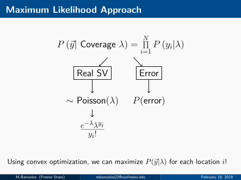
Maximum Likelihood Approach
P (~y| Coverage λ) =N∏i=1
P (yi|λ)
Real SV Error
∼ Poisson(λ) P (error)
e−λλyiyi!
Using convex optimization, we can maximize P (~y|λ) for each location i!
M.Banuelos (Fresno State) [email protected] February 18, 2019
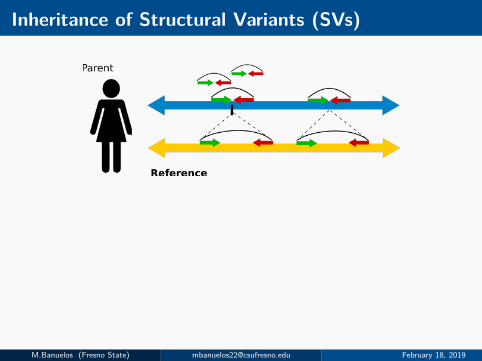
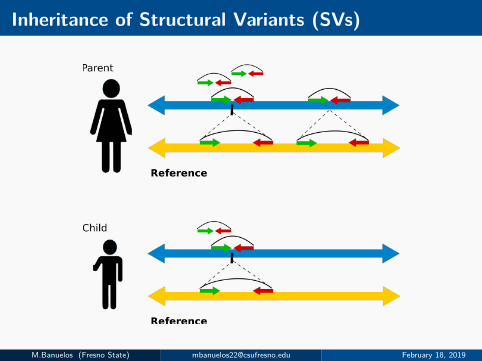
Inheritance of Structural Variants (SVs)
M.Banuelos (Fresno State) [email protected] February 18, 2019
Inheritance of Structural Variants (SVs)
M.Banuelos (Fresno State) [email protected] February 18, 2019
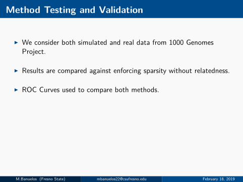
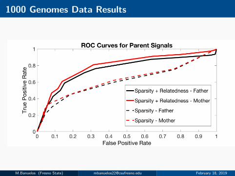
Method Testing and Validation
I We consider both simulated and real data from 1000 GenomesProject.
I Results are compared against enforcing sparsity without relatedness.
I ROC Curves used to compare both methods.
M.Banuelos (Fresno State) [email protected] February 18, 2019
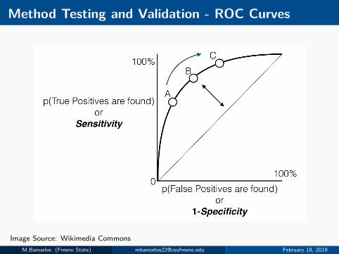
Method Testing and Validation - ROC Curves
Image Source: Wikimedia CommonsM.Banuelos (Fresno State) [email protected] February 18, 2019
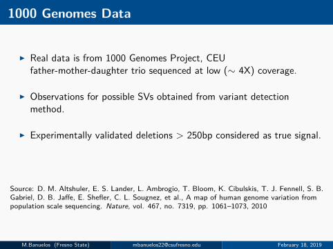
1000 Genomes Data
I Real data is from 1000 Genomes Project, CEUfather-mother-daughter trio sequenced at low (∼ 4X) coverage.
I Observations for possible SVs obtained from variant detectionmethod.
I Experimentally validated deletions > 250bp considered as true signal.
Source: D. M. Altshuler, E. S. Lander, L. Ambrogio, T. Bloom, K. Cibulskis, T. J. Fennell, S. B.Gabriel, D. B. Jaffe, E. Shefler, C. L. Sougnez, et al., A map of human genome variation frompopulation scale sequencing. Nature, vol. 467, no. 7319, pp. 1061–1073, 2010
M.Banuelos (Fresno State) [email protected] February 18, 2019
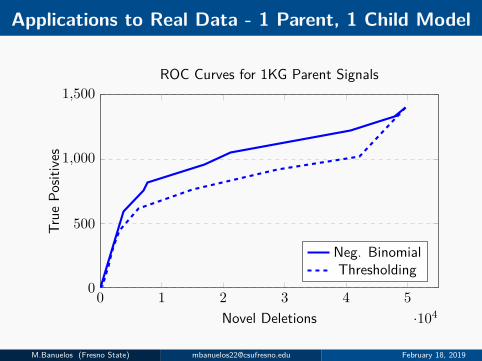
Applications to Real Data - 1 Parent, 1 Child Model
0 1 2 3 4 5·104
0
500
1,000
1,500
Novel Deletions
True
Posit
ives
ROC Curves for 1KG Parent Signals
Neg. BinomialThresholding
M.Banuelos (Fresno State) [email protected] February 18, 2019

Conclusions
I There are plenty of areas you can apply your mathematics andstatistics backgrounds (this is just a sample).
I I like to work with data.I I like to work with data. I like to work with low-quality data.I If you are around next semester and this is interesting, shoot me an
email.
M.Banuelos (Fresno State) [email protected] February 18, 2019
Conclusions
I There are plenty of areas you can apply your mathematics andstatistics backgrounds (this is just a sample).
I I like to work with data.
I I like to work with data. I like to work with low-quality data.I If you are around next semester and this is interesting, shoot me an
email.
M.Banuelos (Fresno State) [email protected] February 18, 2019
Conclusions
I There are plenty of areas you can apply your mathematics andstatistics backgrounds (this is just a sample).
I I like to work with data.I I like to work with data. I like to work with low-quality data.
I If you are around next semester and this is interesting, shoot me anemail.
M.Banuelos (Fresno State) [email protected] February 18, 2019
Conclusions
I There are plenty of areas you can apply your mathematics andstatistics backgrounds (this is just a sample).
I I like to work with data.I I like to work with data. I like to work with low-quality data.I If you are around next semester and this is interesting, shoot me an
email.
M.Banuelos (Fresno State) [email protected] February 18, 2019


![Methods in Cell Biology PDF[1]](https://static.fdocuments.net/doc/165x107/546aff5faf795980298b49d5/methods-in-cell-biology-pdf1.jpg)