Machine Learning for Intraday Returns Forecasting in the ...

UNIVERSIDADE DE SÃO PAULO

FACULDADE DE ECONOMIA, ADMINISTRAÇÃO E CONTABILIDADE

DEPARTAMENTO DE ECONOMIA

PROGRAMA DE PÓS-GRADUAÇÃO EM ECONOMIA

Machine Learning for Intraday Returns Forecasting in

the Brazilian Stock Market

Machine Learning para previsão intraday de retornos no mercado acionário

brasileiro

Henrique Leone Alexandre

Orientador: Prof. Dr. Alan De Genaro

São Paulo

2020

Prof. Dr. Vahan Agopyan

Reitor da Universidade de São Paulo

Prof. Dr. Fábio Frezatti

Diretor da Faculdade de Economia, Administração eContabilidade

Prof. Dr. José Carlos de Souza Santos

Chefe do Departamento de Economia

Prof. Dr. Ariaster Baumgratz

Chimeli Coordenador do Programa de Pós-Graduação emEconomia

Henrique Leone Alexandre

Machine Learning for Intraday Returns Forecasting in

the Brazilian Stock Market

Machine Learning para previsão intraday de retornos no mercado acionário

brasileiro

Dissertação apresentada ao Programa

de Pós-Graduação em Economia do De-

partamento de Economia da Faculdade

de Economia, Administração e Contabil-

idade da Universidade de São Paulo,

como requisito parcial para a obtenção

do título de Mestre em Ciências.

Orientador: Prof. Dr. Alan De Genaro

Versão original

São Paulo

2020

Agradecimentos

Agradeço à minha família que desde sempre incentivou e apoiou minhas decisões,

tornando mais leve, não apenas esta etapa da minha vida, mas todas pelas quais passei

até hoje. Em especial, agradeço à minha mãe que me acompanhou em cada alegria e

tristeza dessa jornada e que, se não fosse por ela, muito provavelmente eu não teria sequer

chegado até aqui.

À minha namorada que esteve sempre ao meu lado, me trazendo paz mesmo nos

momentos mais difíceis do caminho.

Ao meu orientador, Alan de Genaro, por todo apoio e dedicação na orientação desse

trabalho.

O presente trabalho foi realizado com apoio da Coordenação de Aperfeiçoamento de

Pessoal de Nível Superior - Brasil (CAPES) - Código de Financiamento 001.

3

Abstract

This paper applies different estimation methods, specialized in dealing with high data

dimensionality, to make rolling five-minute-ahead return forecasts using high frequency

data, 5 minutes. The methods used are ridge, LASSO, elastic net, PCR and PLS. The

explanatory variables are only the lagged returns of their own and of all the other stocks on

the Ibovespa index. More than just statistical, the economic sense behind these variables

is that they can quickly capture the impact of new information about the companies.

The aim of this paper is to perform a comprehensive comparison of out-of-sample forecast

performance of stock returns among methods. The results show that Ridge Regression

produces the best performance among all methods with a significant advantage. To assess

the robustness of the results, different portfolios were formed. The returns obtained

for the portfolio built with the most volatiles stocks and the portfolio that exploits the

predictability of machine learning methods, even under a conservative assumption on

transaction cost, suggest that these approaches appear to be promising for traders.

Keywords: Machine Learning, Ridge, Lasso, Elastic Net, PCR, PLS

Resumo

Esse trabalho aplica diferentes métodos de estimação, especializados em lidar com

alta dimensionalidade dos dados, em janelas móveis para realizar previsões de retorno

um passo a frente utilizando dados de alta frequência, 5 minutos. Os métodos utilizados

são o ridge, LASSO, elastic net, PCR e PLS. As variáveis explicativas são apenas os

retornos defasados da própria e de outras ações presentes no índice Ibovespa. Mais que

somente estatísticos, o sentido econômico por trás dessas variáveis é que elas tornam

possível capturar, de forma rápida, o impacto de novas informações sobre as empresas.

O objetivo deste trabalho é realizar uma comparação do desempenho para previsão de

retornos fora da amostra entre os métodos citados. Os resultados mostram que o Ridge

produz o melhor desempenho entre todos os métodos, com uma vantagem significativa.

Para avaliar a robustez dos resultados, foram formadas diferentes carteiras. Os retornos

obtidos para o portfólio composto pelas ações mais voláteis e para o portfólio que explora

a previsibilidade dos métodos de machine learning, mesmo sob uma premissa conservadora

sobre o custo da transação, sugerem que essas abordagens parecem promissoras para serem

aplicadas por traders.

Palavras-Chave: Machine Learning, Ridge, Lasso, Elastic Net, PCR, PLS

Contents

1 Introduction 7

2 Literature 10

3 Methodology 14

3.1 Ordinary Least Squares (OLS) . . . . . . . . . . . . . . . . . . . . . . . . . 14

3.1.1 Extension: Huber Function . . . . . . . . . . . . . . . . . . . . . . 15

3.2 Penalized Regression . . . . . . . . . . . . . . . . . . . . . . . . . . . . . . 16

3.2.1 Ridge . . . . . . . . . . . . . . . . . . . . . . . . . . . . . . . . . . 16

3.2.2 LASSO . . . . . . . . . . . . . . . . . . . . . . . . . . . . . . . . . 18

3.2.3 Elastic Net . . . . . . . . . . . . . . . . . . . . . . . . . . . . . . . 19

3.3 Dimension reduction methods . . . . . . . . . . . . . . . . . . . . . . . . . 21

3.3.1 Principal Component Regression (PCR) . . . . . . . . . . . . . . . 21

3.3.2 Partial Least Squares (PLS) . . . . . . . . . . . . . . . . . . . . . . 23

4 Implementation 24

4.1 Data . . . . . . . . . . . . . . . . . . . . . . . . . . . . . . . . . . . . . . . 24

4.2 Estimation . . . . . . . . . . . . . . . . . . . . . . . . . . . . . . . . . . . . 24

4.3 Cross-Validation and Hyperparameters . . . . . . . . . . . . . . . . . . . . 25

4.4 Comparison of Results . . . . . . . . . . . . . . . . . . . . . . . . . . . . . 27

4.4.1 RMSE . . . . . . . . . . . . . . . . . . . . . . . . . . . . . . . . . . 27

4.4.2 Model Confidence Set . . . . . . . . . . . . . . . . . . . . . . . . . . 28

4.4.3 Trading Strategy . . . . . . . . . . . . . . . . . . . . . . . . . . . . 29

5 Results 32

5.1 General analysis using RMSE . . . . . . . . . . . . . . . . . . . . . . . . . 32

5.2 Model Complexity . . . . . . . . . . . . . . . . . . . . . . . . . . . . . . . 36

5.3 Model Confidence Set . . . . . . . . . . . . . . . . . . . . . . . . . . . . . . 37

5.4 Trading Strategy . . . . . . . . . . . . . . . . . . . . . . . . . . . . . . . . 38

5.4.1 Equal Weighted Portfolio . . . . . . . . . . . . . . . . . . . . . . . 39

5.4.2 Weights Mimicking Ibovespa . . . . . . . . . . . . . . . . . . . . . . 40

5.4.3 Volatility and Volume Portfolios . . . . . . . . . . . . . . . . . . . . 42

5.4.4 Machine Learning Portfolio . . . . . . . . . . . . . . . . . . . . . . 46

5

5.4.5 Strategy Robustness . . . . . . . . . . . . . . . . . . . . . . . . . . 50

5.4.6 Tuning The Strategy . . . . . . . . . . . . . . . . . . . . . . . . . . 52

6 Conclusion 54

7 References 55

8 Apendix 59

6

1 Introduction

Forecasting stock returns is a research topic that has received great attention for

decades. For academics, recent advances in this research agenda make it possible, for

example, to test market efficiency or use these results to produce or improve asset pric-

ing models. For practitioner, advances are also important, as they allow, for example,

to improve portfolio allocation and to exploit predictability, if any, to increase trading

profitability.

An important point to consider in this context is the hypothesis of efficient markets.

Until the 1980s, models considered that the expected return was constant, therefore,

predictability invalidated this hypothesis. However, a number of empirical evidences have

begun to show that stock return prediction is possible using the most diverse variables.

To accommodate these advances, Fama (1991) proposed that the expected returns should

be considered as variable along time. Over the last few years, several general equilibrium

models have incorporated the idea proposed by Fama, and making return predictability

possible. Some examples are the papers of Campbell and Cochrane (1999) and Bansal

and Yaron (2004).

Despite the importance of better understanding the return forecasting process, Goyal

and Welch (2008) show that this is not an easy task. They analyze the performance of

several variables suggested by the literature as good predictors for the expected returns

during the period from 1975 to 2005. The results obtained were that, with the exception

of one, the performance of the models proposed for the forecast objective were poor,

both inside and outside the sample. Many of them were not even better than using the

historical average. Finally, they suggest that researchers should wait for more available

data or use more sophisticated models.

Fortunately, the directions suggested by Goyal and Welch (2008) have been followed

and the stock return forecasting literature has been evolving rapidly. This is largely due

to increased computing power, more data availability, and better modeling techniques.

Recently, several studies have been able to perform better than the historical average for

out-of-sample data.

In addition, competition among finance professionals means that once a profitable

strategy is discovered everyone will use it so that it is no longer possible to profit. The

paper of McLean and Pontiff (2015) shows this fact, it analyzes what happens to the

7

predictability of returns after the publication of some strategy. Their conclusion is that

returns decrease by around 35% after publication, and this is due to the pricing problems

by agents.

The stock return prediction literature is divided into two types of approaches. The first

is to analyze the differences in returns between stocks using characteristics, or factors, of

each company. The traditional approach is to run cross-section regressions of the returns

with respect to these lagged features.

In this context, the paper that received great attention and encouraged the search

for new factors was that of Fama and French (1992). They analyzed some anomalies

that improved the predictive power of CAPM, the model that was generally used at the

time. Since then, the literature has increasingly found statistically significant factors. For

example, Harvey, Liu and Zhu (2016) use 316 different factors which, according to them,

were chosen from careful analysis.

The second type of approach is to forecasts the time series of returns. In this case, a

traditional approach is defined as regressions of returns relative to macroeconomic vari-

ables such as nominal interest rates (Ang and Bekaert, 2007), inflation (Campbell and

Vuolteenaho, 2004), market volatility (Guo, 2006). and output gap (Cooper and Priestly,

2009).

In both cross-section and time series, while statistically significant variables increased,

there was a growing increase in the number of variables considered in the modeling.

This issue has been widely discussed in the literature. Cochrane (2011) recognizes this

multidimensional difficulty and establishes as the main challenge for researchers to find

the variables that independently explain the expected returns taking into account the

correlation structure between them. He still compares this situation with that previously

reported in the Fama and French (1992) publication, "We are going to have to repeat

Fame and French’s anomaly digestion, but with many more dimensions".

Besides Cochrane (2011), Harvey, Liu and Zhu (2016) reinforce the need to use new

methodologies and methods. They conclude that given hundreds of publications and fac-

tors, many of the findings in the asset pricing literature are actually false discoveries. The

authors find that, given the high number of factors, many of the historically discovered

factors would be considered significant by chance. To overcome this issue they recom-

mends: (i) the adoption of multiple hypotheses testing framework or (ii) Out-of-sample

8

approach. According to them, when feasible, out-of-sample testing is the cleanest way to

rule out spurious factors.

More recently, Feng, Giglio and Xiu (2020) proposed a methodology to try to organize

what they call a “zoo of factors”. The objective is not only to identify useful and redundant

factors, but also to define a systematic way of testing new possible factors. Despite the

importance of this type of analysis, it does not consider variables that may be relevant

but disappear quickly. Therefore, a relevant source of information may be being ignored.

This paper seeks to mitigate these problems discussed in the return prediction lit-

erature, such as poor out-of-sample performance, data multidimensionality, short-lived

signals and the need for new methodologies, through machine learning methods.

9

2 Literature

Even though macroeconomic variables are predominant in the time series approach, an

alternative that has shown significant results is to use the past returns in different ways.

The Table 1 below presents a sample of studies conducted to assess the predictability

performance of stock price returns.

Paper Method Frequency Asset Country

Jegadeesh (1990) OLS Monthly NYSE (Stocks) US

Lo and MacKinlay (1990) OLS Weekly NYSE (Stocks) US

Brennan, Bhaskaran and Jegadeesh(1993) OLS Daily NASDAQ (Stocks) US

Rapach (2013) OLS, LASSO, Elastic net MonthlyASX, TSX, CAC 40, CDAX, FTSE MIB,

Nikkei, Euronext, OMXS30, SIX,FTSE, S&P 500 (Indices)

AU, CA, FR, DE,IT, JP, NL, SE,CH, UK and US

Chinco, Clark-Joseph and Ye (2019) LASSO 1 minute NYSE (Stocks) US

Gu, Kelly and Shiu (2020) OLS, LASSO, Elastic net,PCR, PLS, NN e RF Monthly NYSE, AMEX, and NASDAQ

(Stocks) US

Table 1: Main articles and their main features

The use of the past returns was initially followed by Jegadeesh (1990) and Lehmann

(1990), who seek to understand the predictability of returns over periods of one week to one

month. Between 1929 and 1989, Jegadeesh (1990) finds that first-order autocorrelation

of monthly returns is negative and statistically significant and that it is positive in larger

orders. He then predicted returns and sorted them into ten portfolios in descending order.

Their results were that the best portfolios had significant gains. Likewise, Lehmann (1990)

notes that when the return in one week is positive it will probably be negative in the next

and also that the opposite is true. With this idea, he builds a zero-cost portfolio and

shows that it generates a positive return in 90% of the weeks, even after discounting

transaction costs.

Instead of using past returns, some studies also use returns from other stocks in the

analysis. Lo and MacKinlay (1990) show that returns from a portfolio composed only of

large companies explain the returns of a portfolio composed only of small companies, but

the opposite does not happen. The idea behind this is that some stocks react faster than

others to new information, in this case, the larger company stocks seem to react faster

than smaller ones.

Brennan, Bhaskaran and Jegadeesh (1993) suggest that this difference in the speed

of price adjustment of a stock can be understood by the number of analysts following

that stock. They find that portfolio returns that many analysts track are important in

10

predicting portfolio returns with fewer analysts. Their conclusion is that the number of

analysts is important to understand which portfolio reacts faster to new information.

For the Brazilian market, Minardi (2004) uses the same methodology as Jegadeesh

(1990) and concludes that past returns have predictive powers for future returns. A

possible explanation given by her is related to the behavior of investors, where they do

not react rationally to new information.

In this context, in contrast to a large number of studies using low frequency, Chinco,

Joseph and Ye (2017) perform this study for high frequency data, 1 minute. The idea of

this analysis is that, in the face of a complex and fast financial market, it is very difficult

for researchers to find factors that are intuitive and persistent in this frequency. Thus,

they suggest using past and other company returns as explanatory variables in order to

identify short-lived signals.

Following the reasoning they used for the US market, assuming that lagged returns on

65 stocks up to three periods are used as explanatory variables, this means that at least

65 × 3 = 195 observations are required. Therefore, this means that to use OLS (i.e , n

≥ p) you must wait, to have at least 16 hours and 15 minutes, which is equivalent to 195

observations at a frequency of 5 minutes, in a 7 hour trading session, to identify a signal

that disappears in minutes. Thus, OLS does not suit this specific purpose.

The alternative proposal is the LASSO, which makes analysis possible when the num-

ber of variables is much larger than the observations. They use a 30-minute rolling window

and around 6000 explanatory variables, whereas in OLS it should be less than 30.

Finally, they conclude that LASSO can capture short-lived signals and that it out-

performs the benchmark. In addition, they find that these signals are not statistical

phenomena, they reflect the consequences that news from one firm has on the other. The

reason that makes it possible to capture these signals is that it can identify faster than

investors.

Therefore, these studies show that past returns of itself and other stocks have predictive

power for future returns on different frequencies, 1 minute, weekly, monthly and yearly.

The explanation for this, according to these papers, is that there is a delay in the speed

of investor reaction to new information about firms. For example, in a report about

the fundamentals of one company that may directly impact another, investors do not

immediately realize this effect and it can be explored by the models.

11

Chinco, Joseph and Ye (2019) attribute the good result obtained by LASSO due to its

ability to quickly identify these signs. Recently, several studies have begun using machine

learning methods for two main gains. First, some of them have no estimation difficulties

when the number of variables is much larger than the number of observations. Second,

its main objective is to obtain better predictions, where they allow bias to occur, but in

such a way as to compensate for a drop in variance.

These machine learning methods have been increasingly used in the asset pricing

literature. Rapach (2013) uses LASSO and elastic net to forecast returns from various

countries using lagged returns. Giglio and Xiu (2016) use dimension reduction methods

to verify the contribution of a new variable, given a large number of factors already

observed, to explain the returns. Light, Maslov and Rytchkov (2016) proposed a new way

of estimating returns by applying PLS.

Despite the increase in these studies, the vast majority of them focus on analyzing

only one method. Given this, Gu, Kelly and Shiu (2020) compare the performance of

several machine learning methods (elastic net, PLS, PCR, glm, random forest and neural

networks) to predict monthly returns using as explanatory variables several factors for

each stock. The results obtained were promising, they verify that these models perform

significantly better than those traditionally used for forecasting returns.

For the Brazilian market, a paper that uses different machine learning methods for

forecasting returns is that of Abdenur, Cavalcante and De Losso (2018). This paper was

done as part of a consultancy that aimed to build an optimal portfolio of markowitz for

private firms where there is no price history. They use machine learning to estimate the

variables needed to build this portfolio, such as return and risk, for private stocks using

several factors of the companies. The result was a large increase in R2 from 10% using

linear regression to 45%.

Still for Brazil, the paper by Val, Pinto and Klotzle (2014) presents interesting results

in the context of forecasting returns and volatility. They show that the models that use

intraday data present the best performance, both in and out-of-sample, reinforcing the

idea that they have important information that should not be ignored.

Given the literature presented, the papers that come closest to what will be done here

are those of Chinco, Joseph and Ye (2019) and Gu, Kelly and Shiu (2020). For the first

one a similar approach will be used, that is, the analysis will be done for high frequency

12

data, 5 minutes, and also rolling windows will be used with the intention to include the

latest information to get better predictions. The goal will be the same as the one proposed

by the second paper, which is to compare the performance between the methods.

Despite the similarities, this paper differs significantly from those discussed. It seeks

to contribute to the return prediction literature, using high frequency data, by comparing

the performance of the most widespread machine learning methods. The comparison will

be made using the mean squared error and the model confidence set by Hansen, Lunde

and Nason (2011), which allows not only to identify the superiority of the models like the

Diebold-Mariano test, but also to order them in a range of confidence. In addition, the

predicted returns by the models will be used to apply some trading strategies and their

economic gains will be compared.

Despite a large number of studies on stock return predictability for the U.S. stock

market, the existing literature on the predictability of stock return of non-U.S. markets

has not been extensive. Recently, several studies have begun to recognize the importance

of considering different markets in the analysis, mainly due to the differences between

emerging and developed countries. Hollstein et al. (2020) studied the predictability of

returns for 81 countries and found that it is higher for emerging countries than in developed

countries. Jordan, Vivian and Wohar (2014) investigated the predictability of returns

in 14 European countries, including emerging and developing countries, and concluded

that the results depend directly on the size of the country, liquidity and development.

Narayan and Thuraisamy (2014) analyze the forecast of returns for emerging countries

using macroeconomic and institutional variables and verify evidence of predictability in

at least 15 of the 18 countries studied and also great heterogeneity between countries.

Therefore, this paper seeks to contribute not only to the scarce Brazilian literature of

forecasting returns using high frequency data and machine learning (Perlin and Ramos,

2016), review the Brazilian literature and find that most studies analyze volatility), but

also to the emerging market literature. Finally, this paper also contributes by suggesting

that standard methods to identifying variables to predict returns should be broaden to

cope with short-lived signals that quickly disappear. If they are not taken into account,

an important source of predictability is being ignored.

13

3 Methodology

The main gain of the methods that will be presented in relation to those usually used in

the literature is the ability to decrease overfitting, allowing a better performance for out-of-

sample forecasts. To make this problem clearer, consider the case where the actual model

is parsimonious (few explanatory variables in the model) and many explanatory variables

are available. It is very likely that there is a linear combination of all the variables that

explain the response variable better than a combination of the true variables in the model.

This is not because the model containing all variables better explains the behavior of the

response variable, but because they fit, in addition to the signal, the noise. Therefore, it

is clear that it is an important problem to be considered when there is a large amount of

variables.

3.1 Ordinary Least Squares (OLS)

This method is the one that presents the simplest approach. Although it seems a

disadvantage, its simplicity generates a parsimonious model that makes it ideal as a

way of comparison with others more complex. In practice, it often produces even better

results. Despite these benefits, the problem of this method appears when the independent

variables have a high correlation or when the number of observations is smaller than the

parameters to be estimated. In this case, the parameters found may be unstable or not

unique.

This approach considers that the model to be estimated can be written as a linear

function, i.e.

yi(xi; t) = x′

iβ.

To find the parameter vector β we must minimize the sum of squared residuals, a loss

function of type L2, obtaining the ordinary least squares estimator,

βols = argminβ

{N∑i=1

(yi − β0 −p∑j=1

xijβj)2

}

= (X ′X)−1X ′y.

14

3.1.1 Extension: Huber Function

An alternative approach is important to use in cases where there are outliers. In the

case of the distribution of returns, it is a stylized fact in the literature that the distribution

of these variables have heavy tails. Therefore, a Huber loss function will also be used.

All models used work by minimizing a loss function or maximizing an objective func-

tion. A loss function measures the quality of a model in trying to predict an expected

value. The most commonly used is the mean squared error (MSE), also called L2, which

measures the sum squared of the distance between the realized and the predicted value.

MSE =1

N

N∑i=1

(yi − f(xi))2.

Another loss function used is the mean absolute error (MAE), also known as L1, which

measures the sum of the absolute difference between the realized value and the predicted

one

MAE =1

N

N∑i=1

|yi − f(xi)| .

The choice between these two functions occurs by checking the data. The loss function

of type L1 is preferable when you have outliers in the sample because it assigns a lower

weight to these observations than a function L2. Despite this benefit, the optimization

process of a function of type L1 is more complicated than one of type L2, because its

derivative is not continuous. Therefore, the Huber function appears as an alternative for

these two cases, being a mixture of them. It is quadratic when the errors are small and

absolute when big, being defined as follows

H(y − f(x), δ) =

[y − f(x)]2 if |y − f(x)| ≤ δ

2δ |y − f(x)| − δ2 otherwise

where the δ parameter defines the approach to be used. Choosing this value is important

because it determines what is considered outlier. It is obtained through an optimization

process from the data.

15

The estimator becomes

βOLSH = argminβ

{1

N

N∑i=1

H(yi − f(xi), δ)

}.

3.2 Penalized Regression

In the literature, alternatives to the ordinary least squares method have been proposed

that may have benefits in relation to predictive performance and model interpretation. In

the case of a linear relationship between the variables, OLS will have the lowest possible

bias. If the number of observations n is much larger than the number of p parameters,

it will have a low variance and a good performance. If this difference is small this model

may have a very large variance and result in overfitting, leading to poor performance for

out-of-sample forecasts. Finally, if the number of parameters is greater than the number

of observations, p > n, then this estimator will not be unique and will probably also have

problems with overfitting. To deal with these difficulties, it is possible to use a form of

constraint or shrinkage of the estimated coefficients. In this context, ridge, LASSO and

elastic net are used.

3.2.1 Ridge

In this method proposed by Hoerl and Kennard (1970) the coefficients are obtained by

minimizing an objective function that depends not only on the sum of squared residuals

as in the OLS, but also on the sum of the squares of these coefficients.

βridge = argminβ

{N∑i=1

(yi − β0 −p∑j=1

xijβj)2 + λ

p∑j=1

β2j

}

The second term of this equation is a penalty for the size of the coefficients, which leads to

the shrinking process of the estimated coefficients. With this, we now allow the trade-off

between bias and variance.

The λ parameter is important in this context as it measures the size of the penalty

applied. Intuitively, this parameter is the price you pay to have large coefficients. If

λ = 0 we have the case of OLS where there is no penalty. As this parameter increases,

16

the greater the penalty will be and, therefore, the estimated coefficients will be smaller.

There is a process of shrinking the coefficients towards zero. Moreover, it is clear that

this parameter directly influences the complexity of the model by changing the size of the

coefficients. One way of understanding this is in the case λ → ∞, where the estimated

model will be as simple as possible, with only intercept. Thus, the higher the value of λ

the simpler the model will be.

In addition to the form presented, there is an equivalent representation of the ridge

estimator:

βridge = argminβ

{N∑i=1

(yi − β0 −p∑j=1

xijβj)2

}

subject to

p∑j=1

β2j ≤ t.

Where there is a one-to-one correspondence between t and λ.

One issue that should be considered in the estimation of these penalized models is the

fact that the coefficients are not invariant under scaling of the explanatory variables. This

is important as the penalty is applied to the size of the coefficients. Thus, if there are

variables with different scales, the effect of the penalty is not the same. Therefore, it is

common to make a normalization so that the variables have zero mean and unit variance,

just calculate

x∗ij =xij − xjσj

,

where xj = 1n

∑ni=1 xij and σ

2j =

1n

∑ni=1(xij − xj)2.

Using the matrix form one can solve the two minimization problems to find the ridge

estimator.

βridge = (X ′X + λIp)−1X ′Y.

Comparing this solution with that obtained by OLS, the difference is that here we add a

positive constant to the diagonal of X ′X before inversion. This makes the problem always

non-singular, that is, it always has a solution, even when X ′X has no complete rank in

the presence of multicollinearity. This was the main motivation of Hoerl and Kennard

(1970) in proposing this model.

17

3.2.2 LASSO

This estimation method works similar to the ridge, the only difference is the type of

penalty applied. Instead of a penalty L2,∑p

j=1 β2j , a penalty L1 will be used,

∑pj=1 |βj|.

This problem can be written as

βlasso = argminβ

{N∑i=1

(yi − β0 −p∑j=1

xijβj)2 + λ

p∑j=1

|βj|

},

or, equivalently,

βlasso = argminβ

{N∑i=1

(yi − β0 −p∑j=1

xijβj)2

}

subject to

p∑j=1

|βj| ≤ t.

This modification, although it seems subtle, has important impacts on the solution

of the problem. The L2 penalty applied to the ridge causes the coefficients to shrink,

but does not cause the coefficients to be exactly zero. Although this is not a problem

for forecasting performance, it can compromise the model interpretation by the number

of variables. This is why Tibshirani (1996) suggested using the L1 penalty, because in

addition to shrinking the coefficients also causes some coefficients to be equal to zero. In

other words, it applies a variable selection, where only the most important are kept in the

model.

This difference between penalties can best be understood through geometric argu-

ments. Consider the case where p = 2 to simplify. Using the representation of the

problem with the constraint, it is known that the solution occurs at the point where the

smallest level curve of the sum of squared residuals intersects the region of the constraint.

Figure 1 shows this problem:

A coefficient is exactly zero only if the solution is on one of the axes. Since the

constraint used in Ridge, β21 + β2

2 ≤ t, has the shape of a circle that has no corners, it

is unlikely that any estimate is exactly zero. In contrast, the LASSO constraint, |β1| +

|β2| ≤ t, is a diamond that has corners on the axes, which causes the intersection of the

smallest level curve of the sum of squared residuals, an ellipse, with one of the axes occurs

frequently. For p > 2 the geometric shapes change, but the reasoning is the same.

18

Figure 1: LASSO and ridge minimization process

Finally, Tibshirani (1996) made a comparison of performance between LASSO and

the ridge using simulations. He concluded that performance depends on the number

of variables of the true model and the size of the coefficients, summarizing this in three

different scenarios. First, if the true model is composed of few variables and the coefficients

are large, then LASSO outperforms the ridge. Second, if the number of variables is small

or medium and the coefficients are medium in size, then LASSO performs better than

ridge. Third, if the model has a large number of variables and the coefficients are small,

then the ridge outperforms the LASSO with a good advantage. So it shows that depending

on the number of variables and the size of the coefficients of the true model both LASSO

and ridge have their importance.

3.2.3 Elastic Net

The comparison made by Tibshirani (1996) between LASSO and ridge shows that

none is better than the other in every situation. However, LASSO presents the property

of variable selection which makes it easier to interpret the models. Thus, Zou and Hastie

(2005) proposed a new method that maintains the good performance of LASSO and fixes

some problems. According to them, there are three main limitations of LASSO:

1. When p > n LASSO selects at most n variables.

2. If there is a highly correlated variable group, LASSO selects only one variable from

19

the group and discards the others.

3. For the common case where n > p, in the presence of variables with high correlation,

the ridge presents better performance than LASSO.

Depending on the case, these limitations make the use of LASSO inappropriate. The

importance of the first point is that there may be more than n relevant variables in the

model and, therefore, this may compromise the results. For the second limitation, given

that there is a group of variables with high correlation, if any of these variables is selected

it is interesting to include the whole group, because this can bring more information.

This property present in the ridge, but not in the LASSO, is called by them the grouping

effect1.

The idea of elastic net is to minimize a loss function formed by the convex combination

of the penalties of the ridge and LASSO methods. This combination is interesting because

it manages to obtain the benefits of each one of them and remedy the limitations discussed.

The L1 penalty contributes to the variable selection process, simplifying the model. The

L2 penalty removes the limitation on the number of variables selected, provides a more

stable solution and includes the grouping effect. This problem can be written as

βelastic net = argminβ

{∑i=1

(yi − β0 −p∑j=1

xijβj)2 + λ1

p∑j=1

|βj|+ λ2

p∑j=1

β2j

}.

Again, as in ridge and LASSO, there is an equivalent representation of this estimator

by an optimization problem. To do this, taking α = λ2(λ1+λ2)

the problem becomes

βelastic net = argminβ

{N∑i=1

(yi − β0 −p∑j=1

xijβj)2

}

subject to (1− α)p∑j=1

|βj|+ α

p∑j=1

β2j ≤ t.

That restriction is the penalty of the elastic net. If α = 1 or α = 0, the problem becomes

equivalent to ridge and LASSO, respectively.1If this property is valid, the coefficients obtained from the variables of the group with high correlation

tend to be equal in module.

20

Finally, Zou and Hastie (2005) compare the performance of the methods using the

same examples used by Tibshirani (1996) and include another in which there is a group

of highly correlated variables. They find that in all cases elastic net performs better than

LASSO, even when LASSO is superior to ridge. Elastic net also includes more variables

than LASSO by the grouping effect discussed. In their last example, where there is the

high correlation group, elastic net outperforms all other methods with a great advantage.

Therefore, the elastic net stands out mainly when the variables are highly correlated.

3.3 Dimension reduction methods

Another alternative for dealing with a large number of highly correlated independent

variables is to use techniques to reduce data dimension. The idea is to obtain a new dataset

with less variables, which are obtained from a transformation of the original variables.

Then estimate the model using these variables. The principal components regression and

partial least squares will be the methods used in this context.

3.3.1 Principal Component Regression (PCR)

The idea of this method is to first apply the principal component analysis (PCA)

to obtain the set of transformed variables and then perform an ordinary least squares

regression with these new variables, Massy (1965). This technique consists of finding

linear combinations of the independent variables, known as principal components, that

capture the largest possible variance and thus the most important characteristics of the

original variables. Therefore, it is expected to find a reduced set of variables that best

represents the original dataset. The first principal component is the linear combination

that has the largest possible variance. Then, the next principal components are obtained

from the linear combination that has the largest possible variance and is not correlated

with the previous components.

The first step is to find out what weights should be used in this linear combination.

One way to find the jth combination of weights, wj, is to solve the following optimization

problem

21

wj = argmaxw

V ar(Xw)

subject to w′w = 1,

Cov(Xw,Xwl) = 0, l = 1, 2, ..., j − 1.

It is possible to prove that the solution of this problem is equivalent to finding the eigenvec-

tors of the covariance matrix of the explanatory variables, X ′X, where the jth combination

of weights is the eigenvector associated with the jth largest eigenvalue, Abdi and Williams

(2010). They can be easily found computationally using singular value decomposition.

The next step is to estimate a regression by OLS using as explanatory variables a small

number of principal components that are able to explain most of the data variability. This

is done to reduce the complexity of the model, in the extreme case where all components

are used the result is the same as that obtained by OLS. Thus, the explanatory variables

are the first M principal components Z1, ..., ZM , where Zj = Xwj.

The model that was previously estimated by OLS

Y = Xβ + ε,

becomes

Y = (XWM)βM + ε,

where WM is a p×M matrix with columns equal to w1, w2, ..., wM . Thus, the number of

estimated parameters decreases, the matrix β that was of size p× 1 becomes M × 1.

The gains from using PCR is that since most of the information in X1, ..., Xp is con-

tained in Z1, ..., ZM and M � p variables are used it is possible to achieve better per-

formance than using only ordinary least squares. This is because it is possible to reduce

overfitting and there is no problem of multicollinearity, since the variables are orthogonal.

This method has two points that must be taken into account in the estimation. It

becomes interesting only when few components are sufficient to explain the variation of

explanatory variables. Moreover, the process of obtaining the principal components does

not consider the dependent variable, and therefore, if the direction in which X1, ..., Xp

has the greatest variability has nothing to do with Y the model may not perform well.

22

3.3.2 Partial Least Squares (PLS)

Thinking about the problem that principal component regression does not take into

account the dependent variable in the estimation process, the partial least squares is an

alternative that fixes this. The objective of this estimation method is no longer to choose

a linear combination that maximizes the variance of the independent variables, but to find

the combination that maximizes the covariance with the dependent variable. The idea

is that the components present a large variation and, at the same time, have the largest

possible correlation with the dependent variable.

The jth combination of weights used to calculate the PLS component can be obtained

from the following optimization problem

wj = argmaxw

Cov2(Y,Xw)

subject to w′w = 1,

Cov(Xw,Xwl) = 0, l = 1, 2, ..., j − 1.

The most common way to solve this problem is to use the NIPALS algorithm, Geladi and

Kowalski (1986) explain in detail, or the SIMPLS proposed by De Jong (1993).

Therefore, instead of finding the components that most closely explain the original

dataset as in PCR, the goal of PLS is to find the components that have the highest

correlation with the dependent variable and thus obtain a better forecasting performance.

23

4 Implementation

4.1 Data

The resulting sample is formed by all stocks belonging the Ibovespa, starting in

07/01/2018 and ending in 2/28/2019. The data used are price, volume and weight of

the 65 stocks that compose the Bovespa index and are sampled in time intervals of 5 min-

utes, totalling 11,627 observations for each stock. The data are obtained directly from

the B3 server.

4.2 Estimation

The estimation process is carried out for each Ibovespa stock using rolling windows

of 30 observations, with the idea of capturing the short-lived signals. The explanatory

variables used are the lagged returns of all Ibovespa stocks, including themselves, in up

to three lagged periods2. Thus, the equation to be estimated is the following:

rn,t = αn +65∑n=1

βn,t−1rn,t−1 +65∑n=1

βn,t−2rn,t−2 +65∑n=1

βn,t−3rn,t−3 + εn,t

where n corresponds to the stock and t to time.

For clarity, consider that the frequency is 5 minutes, the first observation occurs when

the market opens at t = 10 : 00, then one should wait 30 observations to make the first

estimation, this corresponds to a period of two hours and twenty five minutes, or until

t = 12 : 25. With the estimated model, the forecast for the next period, corresponding to

t = 12 : 30, is realized using the lagged returns of the last 3 periods.

Figure 2: Rolling window at the beginning of the day

Then, the rolling window will move until the last forecast is at t = 16 : 50 and this2Except OLS-Huber (OLSH) that uses only the return of the own stock

24

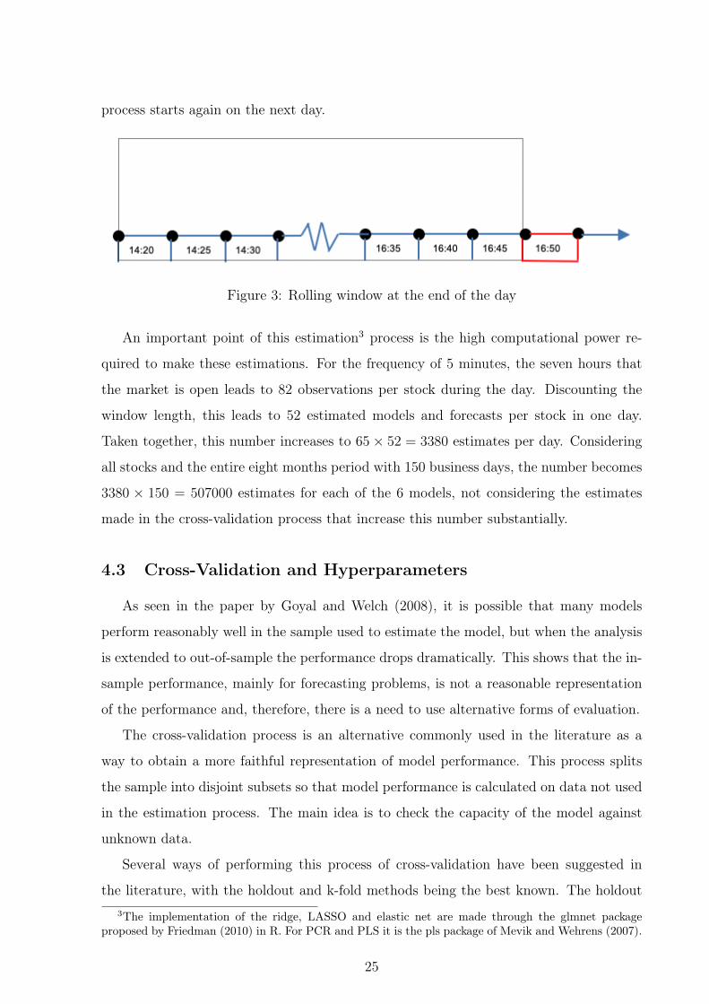
process starts again on the next day.

Figure 3: Rolling window at the end of the day

An important point of this estimation3 process is the high computational power re-

quired to make these estimations. For the frequency of 5 minutes, the seven hours that

the market is open leads to 82 observations per stock during the day. Discounting the

window length, this leads to 52 estimated models and forecasts per stock in one day.

Taken together, this number increases to 65× 52 = 3380 estimates per day. Considering

all stocks and the entire eight months period with 150 business days, the number becomes

3380 × 150 = 507000 estimates for each of the 6 models, not considering the estimates

made in the cross-validation process that increase this number substantially.

4.3 Cross-Validation and Hyperparameters

As seen in the paper by Goyal and Welch (2008), it is possible that many models

perform reasonably well in the sample used to estimate the model, but when the analysis

is extended to out-of-sample the performance drops dramatically. This shows that the in-

sample performance, mainly for forecasting problems, is not a reasonable representation

of the performance and, therefore, there is a need to use alternative forms of evaluation.

The cross-validation process is an alternative commonly used in the literature as a

way to obtain a more faithful representation of model performance. This process splits

the sample into disjoint subsets so that model performance is calculated on data not used

in the estimation process. The main idea is to check the capacity of the model against

unknown data.

Several ways of performing this process of cross-validation have been suggested in

the literature, with the holdout and k-fold methods being the best known. The holdout3The implementation of the ridge, LASSO and elastic net are made through the glmnet package

proposed by Friedman (2010) in R. For PCR and PLS it is the pls package of Mevik and Wehrens (2007).

25

consists of splitting the sample into two subsets, called training and testing. The training

set, which normally consists of 80% of the sample, is used to estimate the models and the

test set, corresponding to the remaining 20%, to evaluate the model performance using

some type of metric, such as mean squared error or absolute error. A major problem with

this method is that this measure of performance can be highly variable according to the

observations included in the training and test set. Moreover, since the estimation process

leaves out a reasonable amount of data, the calculated error tends to be overestimated.

As a way to avoid the problems discussed, k-fold is a widely used alternative. It

consists of randomly splitting the sample into k-sets of equal size. Then, leave one k set

out, estimate the model in the other k − 1 parts (combined), and use that model to get

the predictions for the data in the k set. This is done for each part k = 1, 2, ..., K and

finally calculate the average of these performance metrics obtained. For example, if the

metric is the mean squared error, as used here, the model error is given by

CV(K) =K∑k=1

1

KMSEk

Usually, the values of k used are 5 or 10 because they have a good trade-off between bias

and variance.

This cross-validation process is extremely important in the estimation of machine

learning models, more specifically in the process of finding the best hyperparameters. As

seen previously, the estimation models depend on unknown parameters, for ridge, LASSO

and elastic net is the lambda value, and for PCR and PLS is the number of principal

components. These parameters, also known as hyperparameters, directly influence the

result of the models, so the values used should be chosen carefully. A logical way is to

choose the values such that they minimize the chosen error metric, where the error is

calculated using cross-validation. This process works as follows: first you define a set of

possible hyperparameters, then for each of these values you must calculate the error using

cross-validation, and, finally, the chosen value is the one with the smallest error.

Therefore, this paper uses k-fold cross-validation with k = 10 for the process of choos-

ing hyperparameters, the same way used by Chinco, Clark-Joseph and Ye (2019). This

process occurs in each window, that is, for each new estimation the optimal parameter

value is found again.

26

Figure 4: Process for choosing hyperparameters

4.4 Comparison of Results

This section aims to explain how model performance comparisons are made.

4.4.1 RMSE

The first way to compare the methods is to use the root mean squared error (RMSE).

The RMSE is calculated for each of the n stocks of Ibovespa and each of the methods as

follows

RMSEn,method =

√√√√ T∑t=1

(yn,t+1 − yn,t+1)2

T

where yn,t+1 is the expected return for the next period outside the sample. Thus, the

error is calculated using only out-of-sample observations.

This leads to a total of 65, one per stock, errors for each method. In order to aggregate

these results and provide a comparable basis, these values are averaged for each method,

i.e.

RMSE =65∑n=1

RMSEn,method65

27

This way of comparing, although it seems simple, is usually used in the literature. It

is interesting because it allows an aggregated analysis by method and also a disaggregated

analysis by stock, where the RMSE for a given stock can be compared.

4.4.2 Model Confidence Set

Although RMSE provides a quantitative way of comparing methods, it alone cannot

tell whether one method is statistically better from another. A widely used alternative is

the Diebold-Mariano test that allows you to verify if a specific model is better than any

other. However, more recently, an extension that brings some benefits in relation to this

test has been suggested by Hansen, Lunde and Nason (2011).

The idea of the Model Confidence Set (MCS) is similar to that of a confidence interval,

where MCS is a set that contains the best model with 100(1−α)% confidence, the α used

is equal to 10%. An important point of this test is that the MCS estimation is performed

only once for all models, in contrast the Diebold-Mariano test must be done in pairs

resulting in n(n − 1)/2. Thus, it is estimated 6 more benchmark models to be included

in the analysis, totaling a total of 12 models, in which if Diebold-Mariano were applied

we would have a total of 12(12 − 1)/2 = 66 tests. These benchmark models consist of

estimating each model using the lagged returns up to three periods of the stock itself and

the Ibovespa index as explanatory variables, rather than the past return of all stocks, i.e.

rn,t = αn +3∑i=1

βibov,t−iribov,t−i +3∑i=1

βn,t−irn,t−i + εn,t

The estimation of this benchmark model allows us to test whether it is really necessary

to include the return of all stocks. If the benchmark models and those using all stocks

returns belong to the MCS set this indicates that it cannot be said that they have differ-

ent predictability power and, therefore, it may be preferable to estimate the benchmark

models, as they are simpler and require less computational power for their estimation.

Another advantage of the Model Confidence Set is that it recognizes the data limi-

tation. If the data is informative, MCS will only result in a single model. Otherwise,

non-informative data makes it difficult to compare models, so MCS contains multiple

models. Moreover, it differs from other comparison methods because, in addition to al-

lowing for more than one better model, it provides p-values that may be useful in the

analysis.

28

4.4.3 Trading Strategy

The last way to compare the models is based on the financial gains obtained from

trading strategies using the predicted values of the models. This approach aims to verify

the difference in gains of a trading strategy between the models and also if they make it

possible to profit.

Two trading strategies are used to make this comparison. The only difference between

them is the entry point at which the stock is bought or sold. This strategy basically

consists of buying a stock if the model’s expected return is higher than the transaction

cost, and not buying if the return is lower. The entry point for strategy 1 is the transaction

cost, while strategy 2 is twice the transaction cost. The idea of testing the second strategy

is that this entry point can ensure that the transaction is performed only if it guarantees

the trader’s costs to enter and exit the position, minimizing transaction cost losses. In

this context, strategies 1 and 2 are called, respectively, "one-way" and "round-trip".

Figure 5: Difference between the strategies used

The idea behind this approach is to replicate a real situation where the trader uses

this system to operate in the market so that future information, that is not available at

the time of decision, is not used.

To better understand what is happening in the strategies, each strategy is applied

to long and short separately. To clarify how the strategy works consider the case of the

long strategy, short follows the same scheme but with changed signs. As it is applied

sequentially, there are two possible initial situations, one may be long on the stock or not,

this is defined by what happened in the past period. Two possible situations may occur if

29

it is not purchased, the model’s expected return may be greater than the transaction cost

and the stock is purchased or it is lower than the transaction cost and nothing is done.

If bought, three options may occur, the expected return is greater than the transaction

cost and the position is maintained, the expected return is less than the transaction cost

and the position is undone and, finally, the return is in the range between the range

(−TC, TC), between the red lines on the chart, where you keep bought. The explanation

of using this inactivity interval can be divided into two parts, if the return belongs to the

interval (0, TC) it is more interesting to stay bought because the transaction will have no

transaction cost and the return is positive. In the other part of this range, (−TC, 0), it

is still interesting to stay long because the expected negative return is less than the loss

incurred with the transaction cost.

Figure 6: Possible decisions for the trading strategy

In this type of approach the transaction cost is of extreme importance, it directly

affects the decision to perform an operation and thus the results. The cost used per

transaction consists of the trading and settlement fee charged by B3 for any type of

daytrade transaction, a slippage fee and, for short transactions, the stock rental fee.

The trading and settlement fee is charged according to the volume of day trade per-

formed4, by increasing the volume the value paid decreases. As a conservative way, the

smallest volume range is used, up to 4 million for individuals and 20 million for legal

person, where a fee of approximately 0.024% per transaction is charged, being 0.004%4The appendix figure shows all the possible ranges

30

trading and 0.02% settlement. For comparison purposes, the amount charged in the

biggest volume range is equivalent to 0.016%, i.e. there is a very large difference between

these ranges. Therefore, the presented results of the financial gains can be improved

considering a scenario with a higher financial volume per day due to a lower rate per

transaction.

The second component of the cost is a slippage fee. It occurs in situations where

you get a different price than expected in a trade entry or exit situation. For example,

consider that at the time a purchase order is posted the stock price is $50. Seconds later,

the price rises to $50.10 and the order is placed, so this 10 cent difference is taken into

account by this rate. The value used will be the same as the one proposed by Caldeira

and Moura (2013), which is equal to 0.05%.

The last component, in order to get closer to what happens in practice for short

operations, is a rent rate that is calculated per stock, and not per operation, referring to

2% p.a., also proposed by Caldeira e Moura (2013). Therefore, the rate per operation for

long and short strategies is equal to

TC = 0.024% + 0.05% = 0.029%.

31

5 Results

Results are presented in this section.

5.1 General analysis using RMSE

The process of comparing the models in this paper is tough, as there are many stocks

for each model. For this purpose, the average of the RMSE is used at first because it

allows comparing the models in general.

Ridge PLS PCR Lasso ElasticNet OLS

1.50

1.75

2.00

2.25

2.50

2.75

3.00

RMSE x 100

0

Figure 7: RMSE results from best model to worst

From Figure 7, which provides a summary analysis of the results, it is possible to

see that the model that best fits with a good advantage is the ridge. Next comes PLS,

PCR, LASSO, elastic net and OLS-Huber (OLSH). Although the results are not directly

comparable with the paper of Gu, Kelly and Shiu (2020), because they use a monthly fre-

quency and their explanatory variables are totally different, the results are in agreement.

They find that the dimension reduction models have a good performance and are better

than the elastic net, but they do not consider the case of LASSO and ridge as was done

here.

32

Moreover, understanding OLS-Huber performance in relation to other models is inter-

esting because, in practice, the estimation of these models are more costly, for example,

the computational power required. The results indicate that these models have a higher

performance than the OLS-Huber, a model usually used, and therefore they should be

considered in stock return forecasting problems.

This aggregated analysis is important to understand the general behavior of the meth-

ods. However, although more difficult, it is even more interesting to understand what

happens in a more disaggregated way. This type of analysis allows, for example, to verify

if some model works better for some type of stock. In this context, the RMSE values

obtained in each method for each stock are compared. Figure 8 shows this comparison,

where the horizontal axis represents a specific stock and the vertical axis the value of the

RMSE × 1000.

ABEV3

B3SA3

BBAS3

BBDC3

BBDC4

BBSE3

BRAP4

BRDT3

BRFS3

BRKM5

BRML3

BTOW3

CCRO3

CIEL3

CMIG4

CSAN3

CSNA3

CVCB3

CYRE3

ECOR3

EGIE3

ELET3

ELET6

EMBR3

ENBR3

EQTL3

ESTC3

FLRY3

GGBR4

GOAU4

GOLL4

HYPE3

IGTA3

ITSA4

ITUB4

JBSS3

KLBN11

KROT3

LAME4

LREN3

MGLU3

MRFG3

MRVE3

MULT3

NATU3

PCAR4

PETR3

PETR4

QUAL3

RADL3

RAIL3

RENT3

SANB11

SBSP3

SMLS3

SUZB3

TAEE11

TIMP3

UGPA3

USIM5

VALE3

VIVT4

Stocks

1.50

1.75

2.00

2.25

2.50

2.75

3.00

RMSE x 100

0

ModelRidgePLSPCRLassoElasticNetOLS

Figure 8: RMSE results of the methods per stock

It is possible to realize that, except a few exceptions5, the ordering of the best models

remains between the stocks. This fact shows that the results are relatively stable in the

sense that there is no method that works better for a type of stock. Moreover, this graph

shows that the results vary significantly between stocks, some are up to double the RMSE,5Table 14 in the appendix shows how often each ordering occurred

33

i.e., this indicates that the return of some stocks are easier to predict and others more

difficult.

As a way of trying to identify if there are common factors between the best and worst

forecasting stocks, the stocks are separated in the first and last deciles of the RMSE, which

corresponds to 6 stocks. Volume, volatility and weights in the Ibovespa index are used.

Volume is important because it represents liquidity; it may be that more liquid stocks are

easier to predict. Volatility, on the other hand, can show, for example, that less volatile

stocks are easier to predict. The weights in the ibovespa index may be indicative of the size

of the company and its representation. Thus, tables 2 and 3 show this relationship, but,

instead of the absolute value of these variables, the percentile value is used, facilitating

the interpretation.

Stock RMSE Volume Percentile Volatility Percentile Weight Percentile

VIVT4 1.50 0.19 0.11 0.77ABEV3 1.57 0.95 0.47 0.92ITUB4 1.58 0.94 0.10 1.00VALE3 1.61 0.98 0.02 0.98TAEE11 1.62 0.18 0.19 0.19KLBN11 1.65 0.55 0.35 0.44

Table 2: Characteristics of stocks with lowest RMSE

Stock RMSE Volume Percentile Volatility Percentile Weight Percentile

KROT3 2.56 0.89 0.94 0.63ESTC3 2.67 0.47 0.45 0.31ELET6 2.80 0.42 0.73 0.32BTOW3 2.84 0.31 0.79 0.27ELET3 2.90 0.66 0.32 0.35GOLL4 3.02 0.35 0.77 0.08

Table 3: Characteristics of stocks with higher RMSE

It is possible to verify that the stocks with lower RMSE, or better performance, seem

to be those with the largest volume and Ibovespa weights. This therefore suggests that

forecasting returns works best for more liquid and large company stocks. For stocks

with higher RMSE, although the relationship is not so clear, it seems that the worst

performance happens for stocks with high volatility.

34

To better understand this relationship for all stocks, a pooled regression for RMSE is

estimated using fixed effects by method. The explanatory variables are volume, volatility,

skewness and weights in the Ibovespa. It is important to include skewness because tail

returns can influence forecasting performance, for example, it may happen that these

methods are able to predict these sudden movements and take advantage of them.

Except skewness, all variables are statistically significant. The results of the pooled

regression indicate that the best forecasts are made for stocks with lower liquidity, more

volatile and from larger companies. They differ in part from what has been found in

the literature. According to Gu, Kelly and Shiu (2020, p.45), "Machine learning method

are most valuable for forecasting larger and more liquid stock returns" . Chinco, Clark-

Joseph and Ye (2019, p.23) also find a similar situation, "The results indicates that LASSO

increase out-of-sample fit slightly more for large, liquid and frequently traded stocks" .

Dependent variable: RMSEVariable Coefficient P-Value

Log(Volume) 0.105 0.000

Volatility -0.434 0.000

Weight −0.067 0.000

Skewness 0.175 0.117

Constant 2.32 0.000

R2 0.095

Table 4: Results pooled regression with fixed effect by method

Therefore, this analysis using the root mean squared error as a metric provides im-

portant information for the analysis. First, it shows that models that use all explanatory

variables, ridge and dimension reduction methods, perform better than variable selection

methods. These results are relatively stable between stocks, that is, there are no methods

that work better for a specific stocks. Furthermore, the performance of the methods seems

to vary significantly between stocks. Analyzing the common factors, the results indicate

that forecasting returns works best for more volatile and large company stocks, and that

it works worst for more liquid stocks.

35

5.2 Model Complexity

As discussed, the choice of hyperparameters is essential for model estimation. There-

fore, it is interesting to analyze the result of these values, as they directly influence their

complexity. Figure 9 shows this through the number of coefficients used in each of the

models, the blue line represents the mean over the entire period.

Aug-18

Oct-18

Sep-18

Dec-18

Nov-18 Jul-

18Jan

-19Feb

-190.0

2.5

5.0

7.5

10.0

12.5

Num

ber o

f Com

pone

nts

PCR

Aug-18

Oct-18

Sep-18

Dec-18

Nov-18 Jul-

18Jan

-19Feb

-190

1

2

3

Num

ber o

f Com

pone

nts

PLS

Aug-18

Oct-18

Sep-18

Dec-18

Nov-18 Jul-

18Jan

-19Feb

-19185

190

195

200

205

Num

ber o

f Variables

Ridge

Aug-18

Oct-18

Sep-18

Dec-18

Nov-18 Jul-

18Jan

-19Feb

-19

2

4

6

8

10

Num

ber o

f Variables

Lasso

Aug-18

Oct-18

Sep-18

Dec-18

Nov-18 Jul-

18Jan

-19Feb

-19

5

10

15

20

25

Num

ber o

f Variables

Elastic Net

Aug-18

Oct-18

Sep-18

Dec-18

Nov-18 Jul-

18Jan

-19Feb

-19

0.6

0.7

0.8

0.9

Alpha

Elastic Net

Figure 9: Average of the optimal number of coefficients per method at each time point,the blue line represents the average over the entire period

According to the results obtained from RMSE, the best models (ridge, PLS and PCR)

are those that use information from all variables. This, therefore, indicates that there

are a large number of variables that contain important information for the forecasting

purpose.

This information improves the understanding of why dimension reduction methods

perform well compared to other methods, losing only to the ridge. The average compo-

nents used by PCR and PLS were approximately 6 and 1, respectively, which is relatively

low compared to 195 explanatory variables. This shows, despite the fact that a large

36

number of variables are important, that many of the signals are redundant and possibly

very noisy. Combining these signals into components makes it possible to reduce this

noise and obtain variables that really contain important information.

Although these dimension reduction methods perform better than variable selection

(LASSO and elastic net), they lose significantly to the ridge. This indicates that in

performing this process a lot of relevant information is lost because, in contrast, the ridge

uses all 186 explanatory variables.

In addition, it is interesting to recall the cases where the ridge does better than LASSO

and elastic net in Tibshirani (1996) simulations . This happens, and with great advantage

as seen here, when the real model is composed of a large number of variables with small

coefficients. Thus, when selecting variables many signals are not used when in fact they

seem to be important. Therefore, this may not be a sparse problem as indicated by

Chinco, Clark-Joseph and Ye (2019).

5.3 Model Confidence Set

Although the RMSE provides a good comparison and important information about

model performance, using this approach is not possible to verify whether this superiority is

statistically significant. Thus, the Model Confidence Set is used to make this comparison,

presenting great advantages over the Diebold-Mariano test, usually used in the literature.

In this approach, the best case is when the MCS contain only one model. This is

important because it brings no doubt about the best model, especially considering that

data limitation is taken into account in the process. According to the results obtained,

this happens only if the ridge is the only model that belongs to MCS. If it is not the only

one, it is reasonable to expect PLS and PCR to be part of this set as they perform well.

Besides allowing to make this comparison between the models, the result of this analy-

sis makes it possible to verify if it is really worthwhile, in terms of performance, to include

the return of all stocks in the process. This is possible due to the inclusion of the bench-

mark models discussed earlier. One possible result is that both the ridge using all stocks

and the ridge using only the return of the stock itself and the index belong to the MCS.

If this happens, it indicates that including the return of all stocks does not bring more

benefits than using the benchmark model and therefore, because it is a simpler model,

facilitating functional as well as computational form, it is preferable.

37

Before performing the test containing all possible models it is performed only on the

benchmark model set and only on the interest model set separately. The result is that

the MCS is composed only by the ridge in both cases. Therefore, even using two different

functional forms, ridge performs better than the other methods, reinforcing the idea of

its optimal performance for this type of problem. Then the test is performed for the set

of all models, the result is that only the ridge using the return of all stocks belongs to the

MCS, that is, it presents better performance than the model containing only the return

of the stock itself and of the index.

Finally, this analysis presents extremely important results to understand the difference

in performance of the models. It indicates that, in the context of this paper, the ridge

seems to be the most appropriate model for forecasting returns. Also, including the

lagged return of all stocks, even if more challenging, is interesting because of its higher

performance than the benchmark model.

5.4 Trading Strategy

Finally, the financial gains generated from the trading strategies discussed are used as

a point of comparison between the methods. This approach also makes it possible to verify

whether any of these models generate significant gains and, therefore, are interesting to

apply in practice. This is possible because the strategies work as if in the real world,

using only available data.

As discussed earlier, two strategies are used for this analysis, the one way that guar-

antees only the cost of entering the position, and the round trip that guarantees both the

cost of leaving and entering the position. The results show that the round trip strategy

performs significantly better in all analyzed portfolios. Therefore, the analysis will be

performed using only this strategy.

The application of each strategy is done by stock using the expected returns of a given

method. In other words, for a specific strategy there is the equivalent of 65, one per stock,

applications of that strategy per method. In addition to using the separate long and short

strategies, a long-short strategy that uses both at the same time is applied.

To make a comparison by method it is interesting to group these applications using

different portfolios and compare their performance. Thus, the return on this portfolio is

calculated by

38

rp =65∑n=1

wpn × rn

where wpn is the weight assigned to stock n in the portfolio and rn is the return of some

strategy to stock n.

The results show that the ridge outperformed the other methods with a good margin

in all the analysed portfolios. The rest of the methods showed reasonably worst and close

results for all scenarios. From a financial point of view, the most volatile stock portfolio

and the machine learning portfolio were the best performers. In addition, using the

transaction costs discussed6, these were the only portfolios that presented good returns

and sharpes in a way that is interesting to be applied in a real trading system.

5.4.1 Equal Weighted Portfolio

The first portfolio is composed of all stocks with equal weights, 165. Although it is a

simple application, and perhaps not smart in the sense of maximizing gains, it allows us

to understand how performance between methods varies on average.

ReturnBuy&Hold Ridge PLS PCR LASSO ElasticNet OLSH

Long -8.17 -1.99 -11.10 -12.24 -11.65 -13.75 -15.62

Short - 6.32 -3.55 -4.72 -4.14 -6.36 -8.32

Long-Short - 4.34 -14.14 -16.27 -15.19 -19.12 -22.54Sharpe

Buy&Hold Ridge PLS PCR LASSO ElasticNet OLSHLong -2.02 -1.07 -5.05 -5.47 -5.36 -6.24 -7.14

Short - 1.98 -1.53 -1.96 -1.75 -2.63 -3.36

Long-Short - 1.67 -7.86 -8.47 -8.80 -11.00 -12.50

Table 5: Results for the portfolio with all stocks and equal weights

Table 5 shows the buy and hold returns and those obtained from the application of

the strategies for each method. For the long strategy all methods have negative returns

and, except the ridge, they all have worse returns than buy and hold.

For short and long-short strategies, ridge was the only method that showed positive

returns, which, although not expressive, have low volatility and a good sharpe. The other6The appendix shows the results of the strategies considering the lowest transaction cost ranges

39

July-18

August-18

September-18

October-18

November-18

December-18

January-19

February-19

−20

−15

−10

−5

0

5

Acc

umul

ated

Return

%Long-Short

Strategy

Ibov

Buy&Hold

Ridge

PLS

PCR

Lasso

ElasticNet

OLS

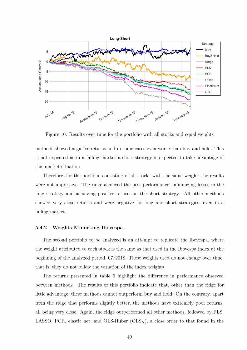
Figure 10: Results over time for the portfolio with all stocks and equal weights

methods showed negative returns and in some cases even worse than buy and hold. This

is not expected as in a falling market a short strategy is expected to take advantage of

this market situation.

Therefore, for the portfolio consisting of all stocks with the same weight, the results

were not impressive. The ridge achieved the best performance, minimizing losses in the

long strategy and achieving positive returns in the short strategy. All other methods

showed very close returns and were negative for long and short strategies, even in a

falling market.

5.4.2 Weights Mimicking Ibovespa

The second portfolio to be analyzed is an attempt to replicate the Ibovespa, where

the weight attributed to each stock is the same as that used in the Ibovespa index at the

beginning of the analyzed period, 07/2018. These weights used do not change over time,

that is, they do not follow the variation of the index weights.

The returns presented in table 6 highlight the difference in performance observed

between methods. The results of this portfolio indicate that, other than the ridge for

little advantage, these methods cannot outperform buy and hold. On the contrary, apart

from the ridge that performs slightly better, the methods have extremely poor returns,

all being very close. Again, the ridge outperformed all other methods, followed by PLS,

LASSO, PCR, elastic net, and OLS-Huber (OLSH), a close order to that found in the

40


Long 0.29 0.53 -8.71 -9.38 -8.21 -10.26 -12.10

SharpeBuy&Hold Ridge PLS PCR LASSO ElasticNet OLSH

Long -0.15 -0.01 -3.51 -3.75 -3.38 -4.06 -4.86

Table 6: Results for the portfolio with weights equal to Ibovespa

July-18

August-18

September-18

October-18

November-18

December-18

January-19

February-19

−20

−15

−10

−5

0

5

Acc

umul

ated

Return

%

Long-ShortStrategy

Ibov

Buy&Hold

Ridge

PLS

PCR

Lasso

ElasticNet

OLS

Figure 11: Results over time for the portfolio with weights equal to Ibovespa

41

RMSE analysis. However, the results were extremely poor in the sense of using these

models to make money.

The result of these two portfolios indicates that these methods seem unable to exploit

the predictability of returns more efficiently than the buy and hold. However, ridge returns

appear to be reasonably promising.

5.4.3 Volatility and Volume Portfolios

Four more portfolios are applied to further analyze the methods. The idea is to try

to explore a group of stocks that make the methods work better. For this, volatility and

volume are used as criteria. The first portfolio trying to explore this idea is composed by

the ten most volatile stocks, i.e. each stock has a weight of 110. The results are presented

in table 7. They seem to show a totally different situation from the previously observed.


Long -19.92 7.31 -6.39 -5.38 -7.95 -10.15 -8.77

Short - 33.39 16.32 17.95 14.47 11.89 13.72

Long-Short - 43.35 9.05 11.77 5.53 0.68 3.91Sharpe

Buy&Hold Ridge PLS PCR LASSO ElasticNet OLSHLong -3.95 2.00 -2.19 -1.80 -2.68 -3.37 -2.90

Short - 7.65 4.00 4.42 3.61 2.98 3.44

Long-Short - 9.27 2.21 2.80 1.34 0.06 0.91

Table 7: Results for top-ten volatile stocks portfolio

The ridge, besides showing again the best performance, presents expressive financial

gains, it generates good returns for all strategies, with emphasis on the long-short that

obtained a 43% return in the period. The most interesting is that this occurs while the

return of buy and hold is approximately -19%, that is, even with the market falling the

long strategy achieved positive returns and the short extracted value from this situation.

The other methods have relatively similar returns between them. Even though they are

significantly worse than the ridge, they are financially interesting as they make it possible

to reduce the loss of long position and are able to extract significant value from the short

position.

42

July-18

August

-18

Septem

ber-18

Octobe

r-18

Novem

ber-18

Decem

ber-18

Januar

y-19

Februa

ry-19

−20

−10

0

10

20

30

40

Accum

ulated

Return %

Long-ShortStrategy

Ibov

Buy&Hold

Ridge

PLS

PCR

Lasso

ElasticNet

OLS

Figure 12: Results over time for top-ten volatile stocks portfolio


Long 0.92 -0.69 -9.72 -12.88 -11.41 -10.86 -13.46

Short - -2.17 -10.98 -14.08 -12.68 -12.09 -14.70

Long-Short - -2.71 -19.52 -25.04 -22.52 -21.52 -26.08Sharpe


Short - -0.75 -3.65 -4.58 -4.12 -4.01 -4.70

Long-Short - -0.90 -6.56 -8.23 -7.77 -7.22 -8.51

Table 8: Results for the least volatile stocks portfolio

43

July-18

August-18

September-18

October-18

November-18

December-18

January-19

February-19

−25

−20

−15

−10

−5

0

5

10A

ccum

ulat

ed R

eturn

%Long-Short

Strategy

Ibov

Buy&Hold

Ridge

PLS

PCR

Lasso

ElasticNet

OLS

Figure 13: Results over time for the least volatile stocks portfolio

When looking at the opposite portfolio, composed of the ten least volatile stocks, the

results are extremely bad even for the ridge. In this scenario, apart from the ridge, the

average returns for the long and short strategies were -13%. This occurs in a market

where buy and hold had positive returns of 0.92%. Ridge had much higher returns than

these other methods, but was still negative and worse than buy and hold. Therefore, this

reinforces the results found in the pooled regression, that the best results are obtained for

the most volatile stocks.


Long -7.69 6.06 -6.15 -8.06 -6.01 -8.63 -10.72

Short - 14.40 1.28 -0.74 1.42 -1.38 -3.65

Long-Short - 21.51 -4.79 -8.60 -4.52 -9.74 -13.85Sharpe

Buy&Hold Ridge PLS PCR LASSO ElasticNet OLSHLong -1.54 1.70 -2.11 -2.74 -2.09 -2.88 -3.58

Short - 3.50 0.23 -0.34 0.26 -0.54 -1.17

Long-Short - 5.12 -1.51 -2.58 -1.47 -3.04 -4.15

Table 9: Results for the most liquid (highest volume) stocks portfolio

Just as these two portfolios were made for volatility, they are also estimated using

volume. The result of the portfolio composed of the ten largest volume stocks shows that,

unlike in the case of volatility, only the ridge stands out. Again, it is able to obtain positive

44

July-18

August-18

September-18

October-18

November-18

December-18

January-19

February-19

−15

−10

−5

0

5

10

15

20

25A

ccum

ulat

ed R

eturn

%Long-Short

Strategy

Ibov

Buy&Hold

Ridge

PLS

PCR

Lasso

ElasticNet

OLS

Figure 14: Results over time for the most liquid (highest volume) stocks portfolio

returns for the long strategy even as the market falls and take significant advantage of

the fall with the short strategy. While all other methods show close and, from a financial

point of view, poor results.

On the other hand, the portfolio formed by the ten stocks with the lowest volume

shows the same thing as the one with the lowest volatility. All methods presented negative

returns and much lower than buy and hold. However, with the exception of the ridge for

higher volume stocks, neither of these two volume based portfolios seem to have good

results.


Long -6.02 -7.92 -16.21 -13.99 -14.30 -15.45 -18.50

Short - -2.59 -11.48 -8.86 -9.38 -10.43 -13.58

Long-Short - -10.22 -25.76 -21.55 -22.27 -24.20 -29.50Sharpe


Short - -1.09 -4.37 -3.45 -3.57 -4.04 -5.25

Long-Short - -3.59 -9.88 -7.78 -8.40 -9.01 -11.46

Table 10: Results for the least liquid (lowest volume) stocks portfolio

An important point to be analyzed is the intersection of stocks between these two

portfolios that presented the best performance, highest volatility and highest volume.

45

July-18

August

-18

Septem

ber-18

Octobe

r-18

Novem

ber-18

Decem

ber-18

Januar

y-19

Februa

ry-19

−30

−25

−20

−15

−10

−5

0

5

10Accum

ulated

Return %

Long-ShortStrategy

Ibov

Buy&Hold

Ridge

PLS

PCR

Lasso

ElasticNet

OLS

Figure 15: Results over time for the least liquid (lowest volume) stocks portfolio

The only common stocks in both portfolios are CIEL3, USIM5 and KROT3. Looking

at the contribution of the returns of these stocks in each of the portfolios7 to the short

strategy, it can be seen that they represent almost all the gains obtained in the highest

volume portfolio and only half of the gains of the highest volatility portfolio. In the long

strategy this contribution is a bit smaller, but still very significant. These results may

indicate that the higher volume of these stocks is not what is influencing this return,

but the volatility. This can be further corroborated by the results obtained in pooled

regression, where higher volume stocks actually performed worse, not better.

Therefore, these results indicate that the best portfolio is formed by more volatile

stocks. In addition, the financial gains obtained make it interesting to be analyzed for

real applications with the objective of bringing good returns for the investor. Regarding

the methods, the ridge was, again, the one with the highest performance with a good

margin, all the others presented worse and very close results.

5.4.4 Machine Learning Portfolio

Then, instead of testing the performance of predefined portfolios, two portfolios are

formed to explore the predictive power of machine learning methods. These portfolios are

assembled so that they contain only the stocks that will generate the highest expected

return at each period of time.7The appendix contains the stock and return tables for each of these portfolios

46

For this, every five minutes the returns forecast for the next period are calculated and

sorted. From these values, the stocks that will be part of the long portfolio of the next

period are the ten that have the highest expected return. For the short portfolio, the

ten stocks with the lowest expected return. Therefore, these stocks in the portfolio will

change every period according to forecasts.

In addition to selecting the stocks in this portfolio each period, you must define a

weight for each of them. Two different forms of calculation are used to further explore

this portfolio. The first, and simplest, is using equal weights for each of the stocks, 110.

For the second is used a way that stocks with the highest expected return have the highest

weight. The idea is basically to divide the expected return of each stock by the sum of

all the expected returns of the stocks that will compose this portfolio,

wpn =rn

10∑n=1

rn

.

For clarity, consider a portfolio consisting of three stocks where the expected return for

each is equals to: r1 = 0.01, r2 = 0.03 and r3 = 0.01. Then, using this form of calculation,

the weights will be w1 =0.010.05

= 20%, w2 =0.030.05

= 60% and w3 =0.010.05

= 20%.

Table 11 and Figure 16 show the portfolio results using equal weights for all stocks.

The ridge was the only method that showed positive returns, this occurs for the long and

short strategy. Still, it is possible to observe the same pattern that occurred in other cases,

where the ridge presents significantly superior performance than the other methods.

ReturnRidge PLS PCR LASSO ElasticNet OLSH

Long 0.06 -21.97 -20.22 -22.11 -27.52 -25.54Short 19.61 -7.57 -5.04 -7.60 -15.40 -13.77

Long-Short 20.22 -27.64 -27.52 -23.85 -35.41 -38.35Sharpe

Ridge PLS PCR LASSO ElasticNet OLSHLong -0.04 -4.83 -4.32 -4.80 -6.16 -5.40Short 3.31 -1.52 -1.00 -1.50 -3.10 -2.66

Long-Short 3.68 -7.08 -6.81 -5.73 -9.34 -10.51

Table 11: Results for the machine learning portfolio with equal weights for all stocks

The returns from the ridge are promising. The long strategy, despite a cumulative

47

July-18

August

-18

Septem

ber-18

Octobe

r-18

Novem

ber-18

Decem

ber-18

Januar

y-19

Februa

ry-19

−40

−30

−20

−10

0

10

20

Accum

ulated

Retur %

Long-ShortStrategy

Ibov

Ridge

PLS

PCR

Lasso

ElasticNet

OLS

Figure 16: Results over time for the machine learning portfolio with equal weights for allstocks

return of 0.06%, was able to maintain higher returns than the Ibovespa for much of the

period, falling sharply from January8. For the short strategy, the results are expressive,

with a cumulative return of 19.61% and still remained above ibovespa for almost the entire

period. Still, this occurred while the market was rising, the accumulated return of the

ibovespa was around 6%.

Table 12 and figure 17 show the portfolio results using the variable weights. In this

strategy, the results were in general worse than using equal weights. The conclusions

previously obtained remain the same for this strategy. Therefore, this indicates that

using equal weights is preferable to using variable weights.

Finally, this portfolio has maintained the same relationship between the methods as

all the others, that the ridge performs significantly better. An interesting point is that

the short portfolio presented returns much higher than the long one, this happens even

with the market going up.

Although the returns seen here are lower than the returns from the portfolio composed

of the most volatile stocks they are significant, achieving a sharpe of 3.68 for the long-short

strategy. This lower return may be due to higher transaction costs. This occurs because

the stocks that are part of this portfolio change every period and, therefore, making these

exchanges causes higher transaction costs. In addition, like the portfolio formed by the

most volatile stocks, the returns of this portfolio that tries to exploit the predictability8The appendix contains the graph of the results over time for the long and short strategies separated

48

ReturnRidge PLS PCR LASSO ElasticNet OLSH

Long -0.86 -27.88 -24.02 -31.01 -34.24 -23.21Short 19.15 -9.36 -5.01 -18.20 -27.64 -24.85

Long-Short 18.73 -43.21 -34.26 -27.40 -41.90 -52.11Sharpe

Ridge PLS PCR LASSO ElasticNet OLSHLong -0.16 -5.40 -4.54 -6.06 -6.90 -4.11Short 2.76 -1.54 -0.80 -3.14 -5.03 -4.10

Long-Short 2.66 -9.46 -6.62 -5.10 -8.07 -12.28

Table 12: Results for the machine learning portfolio with variable weights

July-18

August-18

September-18

October-18

November-18

December-18

January-19

February-19

−50

−40

−30

−20

−10

0

10

20

30

Accumulated

Return %

Long-ShortStrategy

Ibov

Ridge

PLS

PCR

Lasso

ElasticNet

OLS

Figure 17: Results over time for the machine learning portfolio with variable weights

49

power of machine learning become interesting to be analyzed for real applications.

5.4.5 Strategy Robustness

Even with the good results obtained in the previous analysis, it is important to test

how the strategies behave in different scenarios to check their robustness. This analysis

will be performed in the same way as the previous ones, but using a different period and,

due to the computational costs, only the ridge, the model with better results. The sample

used starts on 01/11/2019 and ends on 05/07/2020, with a total of 73 shares that compose

the Ibovespa Index.

The choice of this period is interesting because we were able to test the strategies

against two completely different market situations. In the first half, it operates high and

with little volatility, given the expectation of Brazil’s economic recovery. In the second

half it operates in sharp decline and high volatility, due to the effect of the coronavirus.

Novem

ber-19

Decem

ber-19

Januar

y-20

Februa

ry-20

March

-20Apr

il-20

May-2

0−30

−25

−20

−15

−10

−5

0

5

10

Acc

umul

ated

Ret

urn

%

Ibovespa IndexStrategy

Ibov

Figure 18: Results over time for the Ibovespa Index

From table 13, which shows the results for this new sample, it is possible to verify

a situation similar to that which was previously confirmed. Not only the best portfolios

remain the most volatile and the machine learning, but also the returns obtained are

significant and greater than previously obtained.

Analyzing the returns of the best strategy from figure 19, it is possible to verify two

interesting things. First, this strategy seems to be robust to different market situations,

50

November

-19

December

-19

Januar

y-20

Februar

y-20

March-2

0April

-20May-

20

0

10

20

30

40

50

Acc

umul

ated

Ret

urn

%Ridge - Top Volatile

Strategy

Long

Short

Long-Short

Figure 19: Results over time for the top volatile portfolio in the new sample

ReturnLong Short Long-Short

Equal Weighted 10.66 -2.15 8.74Weights Mimicking Ibovespa -7.09 -10.94 -16.96

Top Volatile 29.04 20.32 55.95Less Volatile -3.98 -4.17 -7.70Most Liquid 1.96 5.33 7.76Least Liquid 9.08 -6.52 2.32

Machine Learning Equal Weights 32.20 -3.52 30.24Machine Learning Variable Weights 39.33 -7.47 32.04

SharpeLong Short Long-Short

Equal Weighted 1.97 -0.38 1.44Weights Mimicking Ibovespa -1.45 -1.99 -2.92

Top Volatile 4.22 2.53 5.54Less Volatile -0.77 -0.67 -1.11Most Liquid 0.33 0.75 0.96Least Liquid 1.68 -1.25 0.39

Machine Learning Equal Weights 2.99 -0.24 3.19Machine Learning Variable Weights 3.10 -0.55 2.75

Table 13: Results for the ridge regression during the new sample

51

it is possible to observe that in the two different scenarios discussed it manages to ob-

tain significant profits. Second, it appears to benefit from more volatile periods, since a

significant amount of returns are realized in the most volatile period.

Therefore, these results corroborate what was found previously and, in addition, in-

dicate that these strategies are robust not only in different periods of time, but also in

terms of market conditions.

5.4.6 Tuning The Strategy

Given the results obtained and the robustness of the strategies presented, the next step

is to try to refine the strategies to improve the results. Previously, two strategies have

been proposed, "one-way" and "round-trip", where the only difference between them is

the entry point. Both were suggested intuitively, where the first strategy aims to operate

only when the expected return is greater than the transaction cost, and the second only to

operate when the expected return is greater than twice the transaction cost, guaranteeing

the cost entry and exit of the operation.

These threshold values have a great effect on the return of the strategies, since they

define when to enter or exit a position. Therefore, although these suggested values make

sense intuitively, it is interesting to analyze the impact of different values on the return

of the strategies. The idea is that there may be some value that optimizes the gains

generated by the strategy, in the same way that the choice of hyperparameters occurs.

To do this, we will check the impact of different thresholds on the return on the port-

folio composed of the most volatile stocks using the ridge, the best portfolio in previous

analyzes. One hundred different values are tested between 0% and 0.5%, with 0.029%

being the value for the one-way strategy and 0.058% for the round-trip.

Figure 20 shows the results obtained for the first sample used and figure 21 for the

second. Not only the similarity of the sharpe and return between the two periods draws

attention but in both cases the optimal threshold, which generates the best results, is the

same. This optimal value is equal to 0.0455% and corresponds to about 1.6 times the

transaction cost, in relation to 2 times for the round-trip.

A possible interpretation of this value is that when using a threshold of 1.6 times the

transaction cost we become less conservative and improve the results, since to enter a

position we need to offset the entry cost and only part of the exit cost.

52

Therefore, these results show that the previous approach of using the round-trip strat-

egy makes sense, but it is still possible to improve the strategy using the optimal threshold.

Using this value instead of the round-trip one in the first sample makes the return goes

from 43.35% to 46.27% and the sharpe from 9.27 to 9.86. In the second sample the return

goes from 55.25% to 60.40% and the sharpe from 5.54 to 5.86. Although these gains do

not seem to be significant, they correspond to an improvement of 6.7% and 6.3% for the

return and sharpe in the first sample and of 9.3% and 5.7%, respectively, in the second

sample.

0.0 0.1 0.2 0.3 0.4 0.5Threshold %

20

10

0

10

20

30

40

50

60

Long

-Sho

rt Return

OptimalRound-Trip

0.0 0.1 0.2 0.3 0.4 0.5Threshold %

−4

−2

0

2

4

6

8

10

Long

-Sho

rt Sha

rpe

OptimalRound-Trip

Figure 20: Return and sharpe of the long-short strategy applied to the top volatile port-folio using different thresholds in the first sample, starting in 07/01/2018 and ending in02/28/2019

0.0 0.1 0.2 0.3 0.4 0.5Threshold %

−20

−10

0

10

20

30

40

50

60

Long

-Sho

rt Return

OptimalRound-Trip

0.0 0.1 0.2 0.3 0.4 0.5Threshold %

−4

−2

0

2

4

6

Long

-Sho

rt Sha

rpe

OptimalRound-Trip

Figure 21: Return and sharpe of the long-short strategy applied to the top volatile port-folio for different thresholds in the second sample, starting in 11/01/2019 and ending in07/05/2020

53

6 Conclusion

In this paper, a comprehensive performance comparison is made among several ma-

chine learning methods for forecasting stock returns. This is done in a high frequency

context using rolling windows, where the goal is to capture short-lived signals. The meth-

ods used are ideal for this scenario where the number of predictors is much higher than

the number of observations.

The models with the best performance were those that used all available explanatory

variables, ridge, PCR and PLS. This indicates that the problem does not appear to be

sparse, few predictors are important, as discussed by Chinco, Joseph and Ye (2019).

Beyond that, there does not seem to have a method that works best for a specific type

of stock, the ordering of best models has remained stable between stocks. The results

indicate that these methods work best for large, volatile and less liquid stocks.

In a comparison between all methods, and still using benchmark models in the analysis,

the ridge using the return of all stocks as explanatory variables was the best model.

Besides being superior to other methods, the results indicate that including the return of

all other stocks brings prediction gains in relation to a model using only the lagged return

of the stock itself and the index.

Finally, trading strategies are applied to different portfolios. The ridge achieved the

best financial returns with a significant difference, while the other methods performed

worst and close to each other. The portfolio with the most volatile stocks and the portfolio

that tries to exploit the predictive power of these machine learning methods performed

the best in terms of returns and sharpe. The significant results for these portfolios suggest

that these approaches look promising to be applied by traders.

These results bring not only academic but also practical contributions. With better

estimation of these expected returns, it is possible to improve the understanding of the

economic factors behind asset pricing, and thus try to bring theory closer to reality. In

addition, they allow for better portfolio allocations and financial gains. Therefore, the

results obtained show that these machine learning methods can contribute significantly

to this problem of forecasting stock returns.

54

References

[1] Bansal, Ravi and Amir, Yaron (2004). Risks for the Long Run: A Potential Resolution

of Asset Pricing Puzzles. The Journal of Finance, v. 59(4)4 : 1481-1509.

[2] Bekaert, Geert and Ang, Andrew (2007). Stock Return Predictability: Is It There?

Review of Financial Studies, v. 20(3) : 651-707.

[3] Brennan, Michael; Jegadeesh, Narasimhan and Swaminathan, Bhaskaran (1993). In-

vestment Analysis and the Adjustment of Stock Prices to Common Information. The


[4] Campbell, John and Vuolteenaho, Tuomo (2004). Bad Beta, Good Beta. The Amer-

ican Economic Review, v. 94(5) : 1249-1275.

[5] Campbell, John and Cochrane, John (1999). Force of Habit: A Consumption-Based

Explanation of Aggregate Stock Market Behavior. Journal of Political Economy, v.

107(2) : 205-251.

[6] Chinco, Alexander; Clark-Joseph, Adam and Ye, Mao (2019). Sparse Signals in the

Cross-Section of Returns. The Journal of Finance, v. 74(2) : 449-492.

[7] Cochrane, John (2011). Presidential Address: Discount Rates. The Journal of Fi-

nance, v. 66(4) : 1047-1108.

[8] Cooper, Ilan and Priestley, Richard (2009). Time-Varying Risk Premiums and the

Output Gap. The Review of Financial Studies, v. 22(7) : 2801-2833.

[9] Fama, Eugene and French, Kenneth (1992). The Cross-Section of Expected Stock

Returns. The Journal of Finance, v. 47(2) : 427-465.

[10] Fama, Eugene (1991). Efficient Capital Markets: II. The Journal of Finance, v. 46(5)

: 1575-1617.

[11] Friedman, Jerome and Hastie, Trevor and Tibshirani, Rob (2010). Regularization

Paths for Generalized Linear Models via Coordinate Descent. Journal of Statistical

Software, v. 33(1) : 1-22.

55

[12] Giglio, Stefano and Xiu, Dacheng (2016). Asset pricing with omitted factors.Working

Papers, Chicago Booth .

[13] Goyal, Amit and Welch, Ivo (2008). A Comprehensive Look at the Empirical Per-

formance of Equity Premium Prediction. The Review of Financial Studies, v. 21(4)

: 1455-1508.

[14] Gu, Shihao and Kelly, Bryan and Xiu, Dacheng (2020). Empirical Asset Pricing via

Machine Learning. The Review of Financial Studies, v. 33(5) : 2223–2273.

[15] Hansen, Peter and Lunde, Asger and Nason, James (2011). The model confidence

set. Econometrica, v. 79(2) : 453-497.

[16] Harvey, Campbell; Liu, Yan and Zhu, Caroline (2016). . . . and the Cross-Section of

Expected Returns. Review of Financial Studies, v. 29(1) : 5-68.

[17] Hoerl, Arthur and Kennard, Robert (1970). Ridge Regression: Biased Estimation for

Nonorthogonal Problems. Technometrics, v. 12(1) : 55-67.

[18] Hollstein, Fabian; Prokopczuk, Marcel; Tharann, Björn and Wese Simen, Chardin

(2020). Predicting the Equity Premium around the Globe: Comprehensive Evidence

from a Large Sample. Working Papers, SSRN.

[19] Jegadeesh, Narasimhan (1990). Evidence of Predictable Behavior of Security Returns.

The Journal of Finance, v. 45(3) : 881-898.

[20] Jordan, Steven; Vivian, Andrew and Wohar, Mark (2014). Forecasting returns: New

European evidence Journal of Empirical Finance, v. 26(1) : 76-95.

[21] Filho, Elias and Abdenur, Flavio and De Losso, Rodrigo (2018). Machine learning

applied to accounting variables yields the risk-return metrics of private company

portfolios.Working Papers, Department of Economics University of São Paulo (FEA-

USP).

[22] Lehmann, Bruce (1990). Fads, Martingales, and Market Efficiency. The Quarterly

Journal of Economics, v. 105(1) : 1-28.

56

[23] Light, Nathaniel and Maslov, Denys and Rytchkov, Oleg (2017). Aggregation of

Information About the Cross Section of Stock Returns: A Latent Variable Approach.


[24] Lo, Andrew and MacKinlay, Craig (1990). When Are Contrarian Profits Due to Stock

Market Overreaction? The Review of Financial Studies, v. 3(2) : 175-205.

[25] Massy, William (1965). Principal Components Regression in Exploratory Statistical

Research. Journal of the American Statistical Association, v. 60(1) : 234-256.

[26] McLean, David and Pontiff, Jeffrey (2016). Does Academic Research Destroy Stock

Return Predictability? Journal of Finance, v. 71(1) : 5-32.

[27] Mevik, Bjorn and Wehrens, Ron (2007). The pls Package: Principal Component and

Partial Least Squares Regression in R. Journal of Statistical Software, v. 18(2) : 1-23.

[28] Narayan, Paresh; Narayan, Seema and Thuraisamy, Kannan (2014). Forecasting re-

turns: New European evidence Journal of Empirical Finance, v. 19(1) : 77-95.

[29] Perlin, Marcelo and Ramos, Henrique (2016). GetHFData: A R Package for Down-

loading and Aggregating High Frequency Trading Data from Bovespa. Brazilian Re-

view of Finance, v. 14(3) : 443-478.

[30] Minardi, Andrea (2004). Retornos passados prevêem retornos futuros?. RAE

eletrônica., v. 3(2).

[31] Rapach, David; Strauss, Jack and Zhou, Guofu (2013). International Stock Return

Predictability: What Is the Role of the United States? The Journal of Finance, v.

68(4) : 1633-1662.

[32] Tibshirani, Robert (1996). Regression Shrinkage and Selection via the LASSO. Jour-

nal of the Royal Statistical Society, v. 58(1) : 267-288.

[33] Zou, Hui and Hastie, Trevor (2005). Regularization and Variable Selection via the

Elastic Net. Journal of the Royal Statistical Society. Series B (Statistical Methodol-

ogy), v. 67(2) : 301-320.

57

[34] Val, Pinto and Klotzle (2014). Volatility and Return Forecasting with High-Frequency

and GARCH Models: Evidence for the Brazilian Market. Revista Contabilidade e

Finanças, v. 25(65) : 189-201.

[35] Feng, Giglio and Xiu (2020). Taming the Factor Zoo: A Test of New Factors. The

Journal of Finance, v. 75(3).

58

Apendix

Figure 22: Cost ranges charged by B3 according to trading volume

Method Number of ParametersRidge λ = 100LASSO λ = 100

Elastic Net λ = 100, α = 5PCR M = 20PLS M = 20

Table 14: Number of parameters tested in the cross-validation process. The values for λand α are chosen by the glmnet package

1 2 3 4 5 6 Frequency

Ridge PLS PCR LASSO ElasticNet OLSH 35Ridge PLS LASSO PCR ElasticNet OLSH 6Ridge PCR PLS LASSO ElasticNet OLSH 6Ridge PLS PCR LASSO OLSH ElasticNet 5Ridge PLS PCR OLSH LASSO ElasticNet 3Ridge LASSO PLS PCR ElasticNet OLSH 2Ridge PCR PLS LASSO OLSH ElasticNet 1Ridge LASSO PCR PLS ElasticNet OLSH 1Ridge PLS PCR ElasticNet LASSO OLSH 1Ridge PLS LASSO PCR OLSH ElasticNet 1Ridge LASSO ElasticNet PLS PCR OLSH 1

Table 15: Frequency ordering of the best to worst method observed in the RMSE analysis

59

Stock Buy&Hold Ridge PLS PCR LASSO ElasticNet OLSHMRFG3 -61.06 12.70 11.41 11.36 9.10 8.17 8.70GOAU4 -29.92 3.75 2.14 2.31 3.26 1.01 2.19MRVE3 -11.72 1.67 0.31 0.52 0.30 0.01 0.70ECOR3 14.63 3.55 0.43 0.55 -0.16 0.62 0.66KROT3 -19.86 5.67 1.86 1.13 1.96 0.95 0.54USIM5 -24.18 4.19 2.03 1.69 2.08 2.27 1.95CSNA3 -4.15 0.26 -1.53 -1.69 -1.37 -1.21 -3.01TIMP3 6.53 0.39 -0.55 0.80 -0.14 -0.48 0.52CIEL3 -35.92 5.69 4.02 4.74 2.89 2.80 4.71MGLU3 -11.66 -0.92 -0.51 -0.29 -1.11 -0.59 -0.44

Table 16: Short strategy data for the most volatile stocks portfolio. The first column isthe stocks that compose the portfolio, the second is the buy and hold return of that stockthroughout the period, and then the contribution of the cumulative return of that stockto the portfolio according to the method (that is, adding the value of all the rows in theridge column results in the total return of this portfolio, which is in table 8)

Stock Buy&Hold Ridge PLS PCR LASSO ElasticNet OLSHMRFG3 -61.06 -0.95 -1.45 -1.50 -2.39 -2.77 -2.57GOAU4 -29.92 -0.23 -1.38 -1.27 -0.59 -2.20 -1.36MRVE3 -11.72 0.44 -0.79 -0.59 -0.78 -1.05 -0.43ECOR3 14.63 5.74 2.12 2.26 1.41 2.33 2.38KROT3 -19.86 2.77 -0.34 -0.93 -0.23 -1.06 -1.41USIM5 -24.18 0.83 -0.83 -1.08 -0.79 -0.65 -0.88CSNA3 -4.15 -0.02 -1.76 -1.92 -1.61 -1.45 -3.20TIMP3 6.53 1.23 0.20 1.58 0.68 0.31 1.31CIEL3 -35.92 0.23 -0.85 -0.41 -1.60 -1.66 -0.42MGLU3 -11.66 -1.72 -1.34 -1.30 -1.94 -1.58 -1.46

Table 17: Long strategy data for the most volatile stock portfolio

Stock Buy&Hold Ridge PLS PCR LASSO ElasticNet OLSHPETR4 8.03 0.02 -1.43 -2.43 -1.68 -2.40 -2.66VALE3 -12.76 0.27 -0.17 -0.01 -0.65 -0.06 0.33ITSA4 15.13 0.52 -0.90 -1.37 -0.37 0.12 -1.32ABEV3 -2.23 -0.20 -0.02 -0.62 -0.38 -0.78 -1.41ITUB4 20.46 -0.83 -2.33 -1.52 -1.76 -1.40 -2.03USIM5 -24.18 4.19 2.03 1.69 2.08 2.27 1.95CIEL3 -35.92 5.69 4.02 4.74 2.89 2.80 4.71KROT3 -19.86 5.67 1.86 1.13 1.96 0.95 0.54BBDC4 18.81 -1.56 -2.39 -2.08 -2.10 -3.13 -2.46CMIG4 -29.79 2.75 2.12 1.21 2.57 1.59 0.45

Table 18: Short strategy data for the most liquid (highest volume) stocks portfolio

60

Stock Buy&Hold Ridge PLS PCR LASSO ElasticNet OLSHPETR4 8.03 1.09 -0.51 -1.64 -0.82 -1.62 -1.93VALE3 -12.76 -0.92 -1.36 -1.22 -1.75 -1.23 -0.84ITSA4 15.13 2.23 0.57 0.04 1.20 1.73 0.09ABEV3 -2.23 -0.36 -0.18 -0.76 -0.53 -0.92 -1.55ITUB4 20.46 1.13 -0.70 0.28 -0.01 0.43 -0.34USIM5 -24.18 0.83 -0.83 -1.08 -0.79 -0.65 -0.88CIEL3 -35.92 0.23 -0.85 -0.41 -1.60 -1.66 -0.42KROT3 -19.86 2.77 -0.34 -0.93 -0.23 -1.06 -1.41BBDC4 18.81 0.11 -0.89 -0.52 -0.55 -1.79 -0.98CMIG4 -29.79 -0.89 -1.34 -1.99 -1.03 -1.73 -2.54

Table 19: Long strategy data for the most liquid (highest volume) stocks portfolio

61

Stock Ridge PLS PCR LASSO Elastic Net OLSHABEV3 1.53 1.58 1.57 1.57 1.60 1.61B3SA3 2.03 2.07 2.08 2.08 2.08 2.13BBAS3 1.91 1.95 1.96 1.96 1.98 2.01BBDC3 1.85 1.89 1.91 1.90 1.92 1.94BBDC4 1.70 1.75 1.76 1.75 1.77 1.77BBSE3 1.62 1.66 1.67 1.68 1.69 1.70BRAP4 1.93 1.97 1.98 1.99 2.01 2.03BRDT3 2.22 2.27 2.28 2.28 2.29 2.48BRFS3 2.01 2.06 2.07 2.07 2.10 2.10BRKM5 1.70 1.75 1.76 1.76 1.78 1.80BRML3 2.11 2.17 2.17 2.19 2.21 2.21BTOW3 2.77 2.84 2.85 2.83 2.84 2.93CCRO3 2.30 2.36 2.37 2.37 2.40 2.40CIEL3 2.20 2.26 2.26 2.27 2.29 2.31CMIG4 2.22 2.28 2.28 2.30 2.32 2.33CSAN3 2.03 2.08 2.10 2.11 2.12 2.15CSNA3 2.34 2.41 2.42 2.43 2.45 2.47CVCB3 2.03 2.09 2.09 2.10 2.11 2.13CYRE3 2.10 2.15 2.15 2.18 2.19 2.22ECOR3 2.18 2.23 2.23 2.23 2.27 2.28EGIE3 1.69 1.72 1.73 1.73 1.74 1.77ELET3 2.83 2.88 2.91 2.93 2.97 2.95ELET6 2.73 2.79 2.80 2.82 2.85 2.85EMBR3 1.79 1.83 1.84 1.85 1.87 1.88ENBR3 1.67 1.71 1.71 1.73 1.74 1.77EQTL3 1.72 1.76 1.77 1.77 1.79 1.80ESTC3 2.58 2.68 2.66 2.69 2.69 2.75FLRY3 2.07 2.11 2.11 2.13 2.13 2.18GGBR4 2.09 2.14 2.15 2.19 2.19 2.19GOAU4 2.17 2.24 2.24 2.26 2.29 2.27GOLL4 2.94 3.00 3.02 3.04 3.08 3.13HYPE3 1.77 1.80 1.81 1.81 1.83 1.87IGTA3 1.81 1.85 1.86 1.87 1.89 1.89ITSA4 1.71 1.75 1.75 1.76 1.77 1.78ITUB4 1.55 1.58 1.59 1.59 1.60 1.61JBSS3 2.32 2.37 2.37 2.38 2.40 2.44

KLBN11 1.62 1.65 1.65 1.66 1.67 1.69KROT3 2.49 2.55 2.56 2.55 2.58 2.65LAME4 2.13 2.18 2.18 2.19 2.20 2.23LREN3 1.96 2.00 2.01 2.03 2.03 2.05MGLU3 1.97 2.01 2.01 2.04 2.05 2.08MRFG3 2.43 2.48 2.49 2.50 2.51 2.59MRVE3 2.04 2.08 2.09 2.11 2.13 2.14MULT3 1.84 1.87 1.89 1.89 1.91 1.92NATU3 1.94 1.98 1.99 2.01 2.02 2.03PCAR4 1.61 1.66 1.66 1.69 1.71 1.68PETR3 1.93 1.97 1.99 2.00 2.03 2.03PETR4 1.98 2.02 2.04 2.04 2.06 2.13QUAL3 2.32 2.38 2.39 2.38 2.41 2.46RADL3 1.83 1.87 1.87 1.88 1.89 1.93RAIL3 2.14 2.19 2.19 2.22 2.24 2.27RENT3 2.18 2.23 2.25 2.25 2.26 2.30SANB11 1.84 1.89 1.89 1.90 1.92 1.93SBSP3 2.03 2.08 2.09 2.11 2.13 2.13SMLS3 2.40 2.44 2.45 2.46 2.47 2.57SUZB3 2.09 2.13 2.14 2.15 2.17 2.22TAEE11 1.58 1.61 1.62 1.63 1.63 1.66TIMP3 1.66 1.71 1.71 1.73 1.74 1.72UGPA3 2.02 2.07 2.08 2.09 2.11 2.12USIM5 2.39 2.45 2.45 2.46 2.50 2.54VALE3 1.57 1.61 1.61 1.63 1.65 1.65VIVT4 1.46 1.50 1.51 1.51 1.52 1.53

Table 20: RMSE × 1000 of all stocks and methods

62

Stock Buy&Hold Ridge PLS PCR LASSO Elastic Net OLSHABEV3 -2.23 -3.63 -1.79 -7.63 -5.31 -9.18 -15.53B3SA3 -5.04 -5.46 -14.35 -17.51 -0.80 -20.41 -8.43BBAS3 2.97 1.65 -6.35 -13.15 -9.54 7.51 -13.38BBDC3 17.12 19.06 2.62 3.69 -6.58 3.04 -5.87BBDC4 18.81 1.07 -8.91 -5.16 -5.51 -17.88 -9.75BBSE3 -10.56 -10.25 -7.85 -17.00 -18.51 -13.57 -14.36BRAP4 30.50 13.79 9.80 -5.46 9.41 -2.69 -0.01BRDT3 -7.01 7.78 -11.72 -19.10 -17.73 -10.04 -17.84BRFS3 12.80 8.16 19.01 -3.64 1.45 -11.54 -6.91BRKM5 -20.27 -6.76 -17.06 -19.29 -22.22 -25.59 -27.25BRML3 -18.96 -12.52 -6.15 -16.78 -16.36 -22.92 -20.18BTOW3 -25.88 -16.92 -25.84 -33.42 -28.83 -18.23 -40.05CCRO3 -5.55 1.65 -24.34 -12.24 -16.11 -18.21 -4.25CIEL3 -35.92 2.32 -8.51 -4.14 -15.98 -16.59 -4.20CMIG4 -29.79 -8.94 -13.42 -19.94 -10.31 -17.30 -25.45CSAN3 34.54 20.70 0.33 -5.31 -8.43 -11.57 -13.56CSNA3 -4.15 -0.17 -17.63 -19.19 -16.09 -14.52 -31.95CVCB3 6.30 -1.80 -2.26 -12.91 -3.41 -8.39 -14.64CYRE3 -15.55 -13.90 -22.18 -16.37 -25.04 -23.76 -21.29ECOR3 14.63 57.39 21.17 22.58 14.13 23.28 23.84EGIE3 -25.50 -20.14 -30.40 -28.18 -17.25 -20.25 -22.75ELET3 -15.39 -18.56 -33.42 -28.30 -31.35 -33.80 -29.44ELET6 -10.04 -16.05 -20.22 -28.01 -23.27 -29.15 -30.94EMBR3 -11.68 -8.48 -7.66 -7.40 -0.46 -12.18 -21.80ENBR3 -1.47 0.70 -8.02 -2.98 -8.55 -9.77 -17.99EQTL3 -2.80 4.28 -20.80 -12.44 -9.49 -12.94 -12.93ESTC3 0.33 -10.97 -26.79 -22.23 -28.19 -31.90 -30.45FLRY3 -2.89 -7.20 -25.15 -17.30 -20.29 -19.81 -16.44GGBR4 8.77 -6.93 -3.50 -17.91 -9.28 -10.56 -8.49GOAU4 -29.92 -2.29 -13.78 -12.65 -5.90 -21.96 -13.63GOLL4 -18.85 2.29 -16.15 -20.89 -4.93 -26.03 -29.44HYPE3 -13.78 -11.78 -16.63 -14.77 -24.13 -23.01 -27.36IGTA3 9.84 1.99 -1.98 -9.72 5.76 -7.49 -2.90ITSA4 15.13 22.28 5.74 0.36 11.95 17.27 0.90ITUB4 20.46 11.30 -7.03 2.84 -0.12 4.31 -3.39JBSS3 1.51 24.39 11.53 4.81 13.42 11.16 0.70

KLBN11 -15.19 -12.39 -14.80 -22.25 -17.15 -17.06 -17.60KROT3 -19.86 27.72 -3.37 -9.27 -2.32 -10.55 -14.12LAME4 -21.66 -19.30 -20.38 -19.51 -29.99 -19.94 -31.41LREN3 -5.16 -1.40 -5.15 -3.65 -7.90 -15.95 0.34MGLU3 -11.66 -17.19 -13.39 -13.03 -19.39 -15.82 -14.58MRFG3 -61.06 -9.53 -14.47 -14.95 -23.93 -27.70 -25.66MRVE3 -11.72 4.39 -7.88 -5.90 -7.81 -10.50 -4.27MULT3 -14.39 -8.99 3.24 -8.83 -7.45 -9.23 -15.57NATU3 -16.59 -10.25 -20.18 -16.48 -16.77 -19.80 -16.01PCAR4 -0.82 -11.55 -14.83 -8.91 -21.13 -16.62 -23.78PETR3 20.04 0.52 -6.16 -2.81 2.78 -11.91 -11.00PETR4 8.03 10.95 -5.13 -16.44 -8.17 -16.19 -19.29QUAL3 -26.44 -14.51 -17.67 -22.99 -28.01 -28.48 -17.86RADL3 -14.22 -13.14 -17.27 -18.19 -19.93 -20.04 -26.88RAIL3 -22.10 -13.87 -25.79 -18.67 -19.16 -20.89 -36.47RENT3 -5.53 -7.80 -16.33 -28.06 -26.79 -18.18 -29.33SANB11 -1.03 2.29 -20.18 -4.23 -1.63 -17.39 -13.86SBSP3 -17.87 2.44 -10.67 -4.26 -3.02 -6.66 -15.45SMLS3 -12.17 -16.02 -25.90 -11.83 -4.29 -8.68 -14.52SUZB3 -22.56 -0.03 -13.27 -7.19 -12.79 -12.78 -17.53TAEE11 -11.72 -8.00 -10.86 -10.98 -24.64 -17.15 -10.98TIMP3 6.53 12.30 2.03 15.84 6.78 3.11 13.12UGPA3 -12.94 -3.87 -8.24 -20.69 -19.50 -10.99 -13.37USIM5 -24.18 8.34 -8.26 -10.83 -7.92 -6.47 -8.82VALE3 -12.76 -9.16 -13.61 -12.18 -17.47 -12.28 -8.45VIVT4 -21.06 -16.13 -21.49 -23.59 -19.81 -22.35 -22.07

Table 21: Cumulative returns for the long strategy over the entire period, 8 months, forall stocks and methods

63

Stock Buy&Hold Ridge PLS PCR LASSO Elastic Net OLSHABEV3 -2.23 -1.99 -0.20 -6.19 -3.83 -7.75 -14.12B3SA3 -5.04 -2.09 -11.14 -14.42 2.90 -17.40 -5.01BBAS3 2.97 -2.91 -10.50 -16.77 -13.63 3.01 -16.98BBDC3 17.12 0.46 -13.34 -12.48 -21.15 -13.06 -20.57BBDC4 18.81 -15.62 -23.91 -20.79 -21.05 -31.34 -24.59BBSE3 -10.56 -0.36 2.45 -7.73 -9.52 -3.93 -4.86BRAP4 30.50 -14.27 -18.88 -28.70 -17.58 -26.57 -24.51BRDT3 -7.01 12.21 -6.66 -14.55 -12.95 -4.88 -13.28BRFS3 12.80 -5.38 4.39 -15.55 -11.52 -22.27 -18.14BRKM5 -20.27 15.44 1.92 -0.05 -4.47 -7.84 -9.35BRML3 -18.96 6.45 14.02 1.14 1.71 -6.48 -2.79BTOW3 -25.88 9.34 -2.45 -12.30 -6.30 7.61 -21.14CCRO3 -5.55 6.00 -21.04 -9.04 -13.11 -15.27 -0.38CIEL3 -35.92 56.92 40.24 47.37 28.85 27.99 47.10CMIG4 -29.79 27.45 21.23 12.06 25.69 15.90 4.50CSAN3 34.54 -11.32 -26.05 -30.15 -33.14 -35.37 -36.56CSNA3 -4.15 2.63 -15.31 -16.92 -13.72 -12.06 -30.05CVCB3 6.30 -8.90 -9.35 -19.23 -10.38 -15.10 -20.86CYRE3 -15.55 0.31 -8.10 -2.51 -12.62 -11.18 -8.29ECOR3 14.63 35.45 4.29 5.53 -1.64 6.19 6.56EGIE3 -25.50 6.26 -7.55 -4.40 9.31 6.17 2.77ELET3 -15.39 -5.37 -22.71 -16.78 -20.45 -23.25 -18.21ELET6 -10.04 -8.57 -13.14 -21.63 -16.37 -22.82 -24.80EMBR3 -11.68 2.20 3.22 3.53 11.29 -1.82 -12.12ENBR3 -1.47 1.15 -7.51 -2.29 -7.74 -8.99 -17.25EQTL3 -2.80 5.04 -20.18 -11.70 -8.40 -11.85 -11.39ESTC3 0.33 -13.18 -28.70 -24.15 -29.97 -33.68 -32.25FLRY3 -2.89 -5.83 -23.95 -15.94 -18.95 -18.53 -15.09GGBR4 8.77 -15.19 -12.07 -25.13 -17.30 -18.44 -16.67GOAU4 -29.92 37.50 21.39 23.13 32.57 10.07 21.88GOLL4 -18.85 21.34 -0.60 -6.18 12.81 -12.22 -16.32HYPE3 -13.78 1.22 -4.40 -2.15 -13.05 -11.74 -16.61IGTA3 9.84 -7.60 -11.13 -18.39 -4.28 -16.59 -12.42ITSA4 15.13 5.19 -8.99 -13.69 -3.71 1.16 -13.21ITUB4 20.46 -8.28 -23.32 -15.20 -17.64 -13.98 -20.34JBSS3 1.51 18.33 6.86 1.32 9.37 7.22 -2.37

KLBN11 -15.19 2.03 -0.12 -8.87 -2.90 -2.86 -3.44KROT3 -19.86 56.68 18.64 11.34 19.60 9.50 5.36LAME4 -21.66 1.73 0.36 1.39 -11.78 0.85 -13.55LREN3 -5.16 2.57 -1.30 0.30 -4.18 -12.60 4.37MGLU3 -11.66 -9.22 -5.11 -2.92 -11.14 -5.91 -4.41MRFG3 -61.06 127.04 114.07 113.62 90.97 81.68 87.04MRVE3 -11.72 16.69 3.06 5.20 3.04 0.11 7.04MULT3 -14.39 4.88 18.95 5.30 7.00 4.38 -2.50NATU3 -16.59 6.93 -5.46 -0.46 -1.02 -4.76 0.04PCAR4 -0.82 -11.64 -15.91 -9.71 -21.25 -16.72 -24.32PETR3 20.04 -16.25 -21.84 -20.66 -15.51 -27.53 -26.80PETR4 8.03 0.23 -14.32 -24.25 -16.77 -24.00 -26.58QUAL3 -26.44 14.31 9.98 2.74 -4.00 -4.55 9.78RADL3 -14.22 0.34 -4.29 -5.39 -7.63 -7.78 -15.62RAIL3 -22.10 8.18 -6.28 2.60 1.69 0.29 -19.61RENT3 -5.53 -3.86 -12.66 -24.99 -23.67 -14.66 -26.29SANB11 -1.03 2.36 -20.10 -4.17 -1.59 -17.37 -13.84SBSP3 -17.87 23.39 7.64 15.31 16.89 12.42 1.92SMLS3 -12.17 -6.77 -17.76 -2.19 6.26 1.31 -5.17SUZB3 -22.56 26.84 9.35 17.06 10.98 10.98 5.09TAEE11 -11.72 3.40 0.33 0.08 -15.19 -6.92 0.12TIMP3 6.53 3.90 -5.54 8.01 -1.37 -4.78 5.20UGPA3 -12.94 8.59 4.03 -9.82 -8.75 1.03 -1.80USIM5 -24.18 41.94 20.27 16.93 20.79 22.67 19.50VALE3 -12.76 2.72 -1.73 -0.10 -6.54 -0.63 3.32VIVT4 -21.06 5.85 -0.68 -3.69 1.28 -1.83 -1.92

Table 22: Cumulative returns for the short strategy over the entire period, 8 months, forall stocks and methods

64

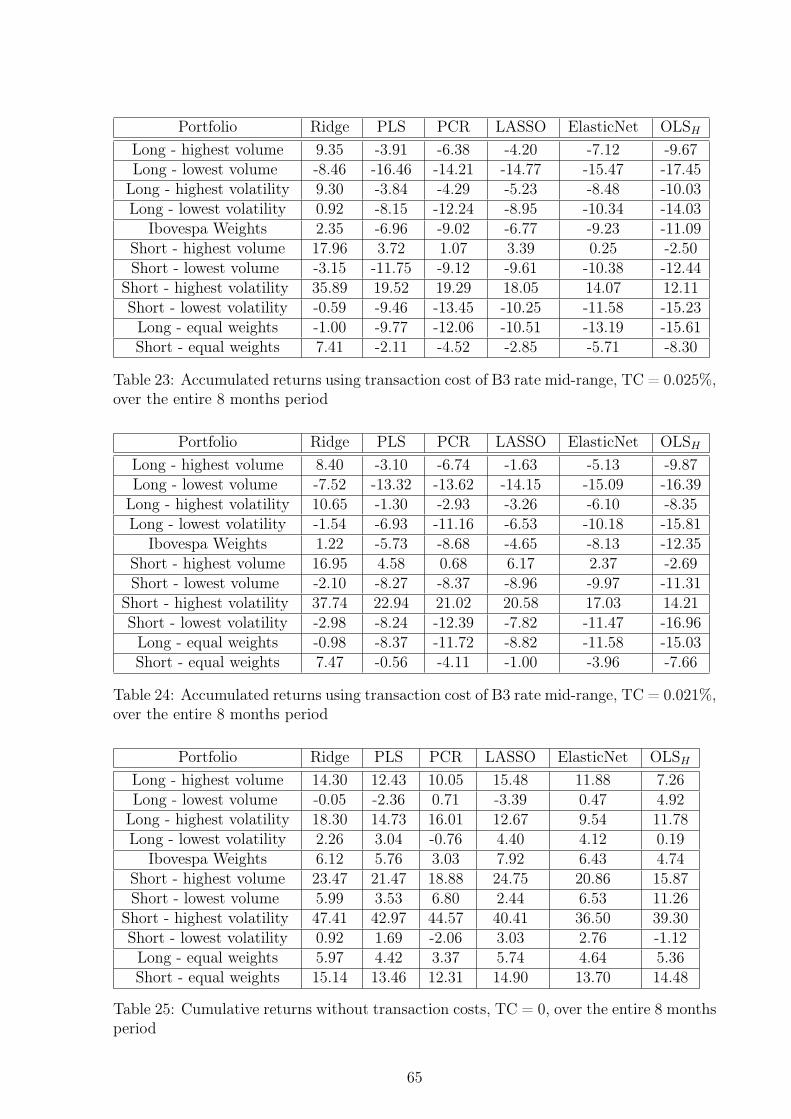
Portfolio Ridge PLS PCR LASSO ElasticNet OLSHLong - highest volume 9.35 -3.91 -6.38 -4.20 -7.12 -9.67Long - lowest volume -8.46 -16.46 -14.21 -14.77 -15.47 -17.45Long - highest volatility 9.30 -3.84 -4.29 -5.23 -8.48 -10.03Long - lowest volatility 0.92 -8.15 -12.24 -8.95 -10.34 -14.03

Ibovespa Weights 2.35 -6.96 -9.02 -6.77 -9.23 -11.09Short - highest volume 17.96 3.72 1.07 3.39 0.25 -2.50Short - lowest volume -3.15 -11.75 -9.12 -9.61 -10.38 -12.44

Short - highest volatility 35.89 19.52 19.29 18.05 14.07 12.11Short - lowest volatility -0.59 -9.46 -13.45 -10.25 -11.58 -15.23Long - equal weights -1.00 -9.77 -12.06 -10.51 -13.19 -15.61Short - equal weights 7.41 -2.11 -4.52 -2.85 -5.71 -8.30

Table 23: Accumulated returns using transaction cost of B3 rate mid-range, TC = 0.025%,over the entire 8 months period

Portfolio Ridge PLS PCR LASSO ElasticNet OLSHLong - highest volume 8.40 -3.10 -6.74 -1.63 -5.13 -9.87Long - lowest volume -7.52 -13.32 -13.62 -14.15 -15.09 -16.39Long - highest volatility 10.65 -1.30 -2.93 -3.26 -6.10 -8.35Long - lowest volatility -1.54 -6.93 -11.16 -6.53 -10.18 -15.81

Ibovespa Weights 1.22 -5.73 -8.68 -4.65 -8.13 -12.35Short - highest volume 16.95 4.58 0.68 6.17 2.37 -2.69Short - lowest volume -2.10 -8.27 -8.37 -8.96 -9.97 -11.31

Short - highest volatility 37.74 22.94 21.02 20.58 17.03 14.21Short - lowest volatility -2.98 -8.24 -12.39 -7.82 -11.47 -16.96Long - equal weights -0.98 -8.37 -11.72 -8.82 -11.58 -15.03Short - equal weights 7.47 -0.56 -4.11 -1.00 -3.96 -7.66

Table 24: Accumulated returns using transaction cost of B3 rate mid-range, TC = 0.021%,over the entire 8 months period

Portfolio Ridge PLS PCR LASSO ElasticNet OLSHLong - highest volume 14.30 12.43 10.05 15.48 11.88 7.26Long - lowest volume -0.05 -2.36 0.71 -3.39 0.47 4.92Long - highest volatility 18.30 14.73 16.01 12.67 9.54 11.78Long - lowest volatility 2.26 3.04 -0.76 4.40 4.12 0.19

Ibovespa Weights 6.12 5.76 3.03 7.92 6.43 4.74Short - highest volume 23.47 21.47 18.88 24.75 20.86 15.87Short - lowest volume 5.99 3.53 6.80 2.44 6.53 11.26

Short - highest volatility 47.41 42.97 44.57 40.41 36.50 39.30Short - lowest volatility 0.92 1.69 -2.06 3.03 2.76 -1.12Long - equal weights 5.97 4.42 3.37 5.74 4.64 5.36Short - equal weights 15.14 13.46 12.31 14.90 13.70 14.48

Table 25: Cumulative returns without transaction costs, TC = 0, over the entire 8 monthsperiod

65

Machine Learning for Intraday Returns Forecasting in the ...

Documents

Transcript of Machine Learning for Intraday Returns Forecasting in the ...