Machine Learning for Fluid Mechanics - arxiv.org

Machine Learning for FluidMechanics

Steven L. Brunton,1 Bernd R. Noack2 3 andPetros Koumoutsakos4

1Mechanical Engineering, University of Washington, Seattle, WA, USA, 981952 LIMSI, CNRS, Universite Paris-Saclay, F-91403 Orsay, France3 Institut fur Stromungsmechanik und Technische Akustik, TU Berlin, D-10634,

Germany4 Professorship for Computational Science, ETH Zurich, CH-8092, Switzerland;

email: [email protected]

Xxxx. Xxx. Xxx. Xxx. YYYY. AA:1–32

https://doi.org/10.1146/((please add

article doi))

Copyright c© YYYY by Annual Reviews.

All rights reserved

Keywords

machine learning, data-driven modeling, optimization, control

Abstract

The field of fluid mechanics is rapidly advancing, driven by unprece-

dented volumes of data from field measurements, experiments and large-

scale simulations at multiple spatiotemporal scales. Machine learning

offers a wealth of techniques to extract information from data that

could be translated into knowledge about the underlying fluid me-

chanics. Moreover, machine learning algorithms can augment domain

knowledge and automate tasks related to flow control and optimiza-

tion. This article presents an overview of past history, current devel-

opments, and emerging opportunities of machine learning for fluid me-

chanics. It outlines fundamental machine learning methodologies and

discusses their uses for understanding, modeling, optimizing, and con-

trolling fluid flows. The strengths and limitations of these methods are

addressed from the perspective of scientific inquiry that considers data

as an inherent part of modeling, experimentation, and simulation. Ma-

chine learning provides a powerful information processing framework

that can enrich, and possibly even transform, current lines of fluid me-

chanics research and industrial applications.

1

arX

iv:1

905.

1107

5v3

[ph

ysic

s.fl

u-dy

n] 4

Jan

202

0

1. INTRODUCTION

Fluid mechanics has traditionally dealt with massive amounts of data from experiments,

field measurements, and large-scale numerical simulations. Big data has been a reality in

fluid mechanics (Pollard et al. 2016) over the last decade due to high-performance comput-

ing architectures and advances in experimental measurement capabilities. Over the past 50

years many techniques were developed to handle data of fluid flows, ranging from advanced

algorithms for data processing and compression, to databases of turbulent flow fields (Perl-

man et al. 2007; Wu & Moin 2008). However, the analysis of fluid mechanics data has relied

,to a large extent, on domain expertise, statistical analysis, and heuristic algorithms.

Massive amounts of data is today widespread across scientific disciplines, and gaining

insight and actionable information from them has become a new mode of scientific inquiry

as well as a commercial opportunity. Our generation is experiencing an unprecedented con-

fluence of 1) vast and increasing volumes of data, 2) advances in computational hardware

and reduced costs for computation, data storage and transfer, 3) powerful algorithms, 4) an

abundance of open source software and benchmark problems, and 5) significant and ongo-

ing investment by industry on data driven problem solving. These advances have, in turn,

fueled renewed interest and progress in the field of machine learning (ML). Machine learn-

ing algorithms (here categorized as supervised, semi-supervised, and unsupervised learning

(see Fig. 1) are rapidly making inroads in fluid mechanics. Machine learning provides a

modular and agile modeling framework that can be tailored to address many challenges

in fluid mechanics, such as reduced-order modeling, experimental data processing, shape

optimization, turbulence closure, and control. As scientific inquiry increasingly shifts from

first principles to data-driven approaches, we may draw a parallel between current efforts

in machine learning with the development of numerical methods in the 1940’s and 1950’s

to solve the equations of fluid dynamics. Fluid mechanics stands to benefit from learning

algorithms and in return present challenges that may further advance these algorithms to

complement human understanding and engineering intuition.

Machine learning:Algorithms thatextract patterns and

information fromdata. They facilitate

automation and can

augment humandomain knowledge.

In this review, in addition to outlining successes, we emphasize the importance of un-

derstanding how learning algorithms work and when these methods succeed or fail. It is

important to balance excitement about the capabilities of machine learning with the reality

that its application to fluid mechanics is an open and challenging field. In this context,

we also highlight the benefit of incorporating domain knowledge about fluid mechanics into

learning algorithms. We envision that the fluid mechanics community can contribute to

advances in machine learning reminiscent of the advances in numerical methods in the last

century.

1.1. Historical Overview

Machine learning and fluid dynamics share a long, and possibly surprising, history of inter-

faces. In the early 1940’s Kolmogorov, a founder of statistical learning theory, considered

turbulence as one of its prime application domains (Kolmogorov 1941). Advances in ma-

chine learning in the 1950’s and 1960’s were characterized by two distinct developments. On

one side we distinguish cybernetics (Wiener 1965) and expert systems designed to emulate

the thinking process of the human brain, and on the other “machines” like the percep-

tron (Rosenblatt 1958) aimed to automate processes such as classification and regression.

Advances on the second branch are also prevailing today and it is understandable how the

use of perceptrons for classification created significant excitement for Artificial Intelligence

2 Brunton, Noack, and Koumoutsakos

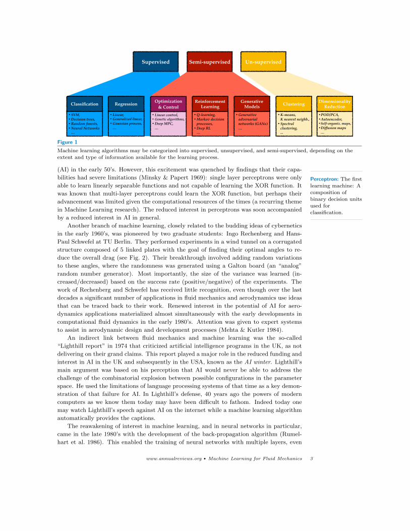
• SVM, • Decision trees,• Random forests,• Neural Networks

…

•POD/PCA,•Autoencoder, •Self-organiz. maps, •Diffusion maps

…

• K-means, K nearest neighb.,

• Spectral clustering,...

• Q-learning, • Markov decision

processes,• Deep RL

…

• Generative adversarial networks (GANs)…

• Linear control,• Genetic algorithms,• Deep MPC,

…

• Linear, • Generalized linear,• Gaussian process,

…

Supervised Semi-supervised Un-supervised

Classification Regression Optimization & Control

Reinforcement Learning

Generative Models Clustering Dimensionality

Reduction

Figure 1

Machine learning algorithms may be categorized into supervised, unsupervised, and semi-supervised, depending on theextent and type of information available for the learning process.

(AI) in the early 50’s. However, this excitement was quenched by findings that their capa-

bilities had severe limitations (Minsky & Papert 1969): single layer perceptrons were only

able to learn linearly separable functions and not capable of learning the XOR function. It

was known that multi-layer perceptrons could learn the XOR function, but perhaps their

advancement was limited given the computational resources of the times (a recurring theme

in Machine Learning research). The reduced interest in perceptrons was soon accompanied

by a reduced interest in AI in general.

Perceptron: The first

learning machine: A

composition ofbinary decision units

used for

classification.

Another branch of machine learning, closely related to the budding ideas of cybernetics

in the early 1960’s, was pioneered by two graduate students: Ingo Rechenberg and Hans-

Paul Schwefel at TU Berlin. They performed experiments in a wind tunnel on a corrugated

structure composed of 5 linked plates with the goal of finding their optimal angles to re-

duce the overall drag (see Fig. 2). Their breakthrough involved adding random variations

to these angles, where the randomness was generated using a Galton board (an “analog”

random number generator). Most importantly, the size of the variance was learned (in-

creased/decreased) based on the success rate (positive/negative) of the experiments. The

work of Rechenberg and Schwefel has received little recognition, even though over the last

decades a significant number of applications in fluid mechanics and aerodynamics use ideas

that can be traced back to their work. Renewed interest in the potential of AI for aero-

dynamics applications materialized almost simultaneously with the early developments in

computational fluid dynamics in the early 1980’s. Attention was given to expert systems

to assist in aerodynamic design and development processes (Mehta & Kutler 1984).

An indirect link between fluid mechanics and machine learning was the so-called

“Lighthill report” in 1974 that criticized artificial intelligence programs in the UK, as not

delivering on their grand claims. This report played a major role in the reduced funding and

interest in AI in the UK and subsequently in the USA, known as the AI winter. Lighthill’s

main argument was based on his perception that AI would never be able to address the

challenge of the combinatorial explosion between possible configurations in the parameter

space. He used the limitations of language processing systems of that time as a key demon-

stration of that failure for AI. In Lighthill’s defense, 40 years ago the powers of modern

computers as we know them today may have been difficult to fathom. Indeed today one

may watch Lighthill’s speech against AI on the internet while a machine learning algorithm

automatically provides the captions.

The reawakening of interest in machine learning, and in neural networks in particular,

came in the late 1980’s with the development of the back-propagation algorithm (Rumel-

hart et al. 1986). This enabled the training of neural networks with multiple layers, even

www.annualreviews.org • Machine Learning for Fluid Mechanics 3

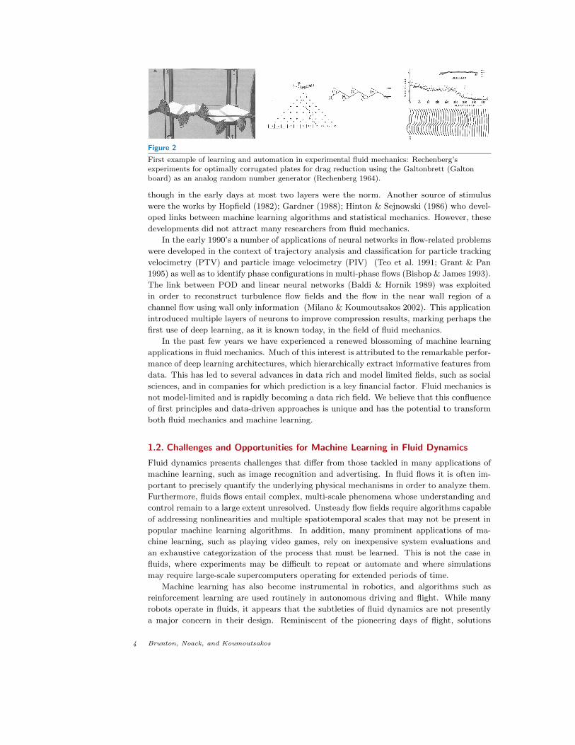
Figure 2

First example of learning and automation in experimental fluid mechanics: Rechenberg’sexperiments for optimally corrugated plates for drag reduction using the Galtonbrett (Galton

board) as an analog random number generator (Rechenberg 1964).

though in the early days at most two layers were the norm. Another source of stimulus

were the works by Hopfield (1982); Gardner (1988); Hinton & Sejnowski (1986) who devel-

oped links between machine learning algorithms and statistical mechanics. However, these

developments did not attract many researchers from fluid mechanics.

In the early 1990’s a number of applications of neural networks in flow-related problems

were developed in the context of trajectory analysis and classification for particle tracking

velocimetry (PTV) and particle image velocimetry (PIV) (Teo et al. 1991; Grant & Pan

1995) as well as to identify phase configurations in multi-phase flows (Bishop & James 1993).

The link between POD and linear neural networks (Baldi & Hornik 1989) was exploited

in order to reconstruct turbulence flow fields and the flow in the near wall region of a

channel flow using wall only information (Milano & Koumoutsakos 2002). This application

introduced multiple layers of neurons to improve compression results, marking perhaps the

first use of deep learning, as it is known today, in the field of fluid mechanics.

In the past few years we have experienced a renewed blossoming of machine learning

applications in fluid mechanics. Much of this interest is attributed to the remarkable perfor-

mance of deep learning architectures, which hierarchically extract informative features from

data. This has led to several advances in data rich and model limited fields, such as social

sciences, and in companies for which prediction is a key financial factor. Fluid mechanics is

not model-limited and is rapidly becoming a data rich field. We believe that this confluence

of first principles and data-driven approaches is unique and has the potential to transform

both fluid mechanics and machine learning.

1.2. Challenges and Opportunities for Machine Learning in Fluid Dynamics

Fluid dynamics presents challenges that differ from those tackled in many applications of

machine learning, such as image recognition and advertising. In fluid flows it is often im-

portant to precisely quantify the underlying physical mechanisms in order to analyze them.

Furthermore, fluids flows entail complex, multi-scale phenomena whose understanding and

control remain to a large extent unresolved. Unsteady flow fields require algorithms capable

of addressing nonlinearities and multiple spatiotemporal scales that may not be present in

popular machine learning algorithms. In addition, many prominent applications of ma-

chine learning, such as playing video games, rely on inexpensive system evaluations and

an exhaustive categorization of the process that must be learned. This is not the case in

fluids, where experiments may be difficult to repeat or automate and where simulations

may require large-scale supercomputers operating for extended periods of time.

Machine learning has also become instrumental in robotics, and algorithms such as

reinforcement learning are used routinely in autonomous driving and flight. While many

robots operate in fluids, it appears that the subtleties of fluid dynamics are not presently

a major concern in their design. Reminiscent of the pioneering days of flight, solutions


imitating natural forms and processes are often the norm (see the sidebar titled ”Learning

Fluid Mechanics: From Living Organisms to Machines”). We believe, that the deeper

understanding and exploitation of fluid mechanics will become critical in the design of

robotic devices, when their energy consumption and reliability in complex flow environments

become a concern.

Interpretability: Thedegree to which a

model may be

understood orinterpreted by an

expert human.

Generalizability: Theability of a model to

generalize to new

examples includingunseen data.

Newton’s second law

is an example.

In the context of flow control, actively or passively manipulating flow dynamics for an

engineering objective may change the nature of the system, making predictions, based on

data of uncontrolled systems, impossible. Although fluid data is vast in some dimensions,

such as spatial resolution, it may be sparse in others; e.g., it may be expensive to perform

parametric studies. Furthermore, fluids data can be highly heterogeneous, requiring special

care when choosing the type of learning machine. In addition, many fluid systems are

non-stationary, and even for stationary flows it may be prohibitively expensive to obtain

statistically converged results.

Fluid dynamics are central to transportation, health, and defense systems, and it is,

therefore, essential that machine learning solutions are interpretable, explainable, and gen-

eralizable. Moreover, it is often necessary to provide guarantees on performance, which are

presently rare. Indeed, there is a poignant lack of convergence results, analysis, and guar-

antees in many machine learning algorithms. It is also important to consider whether the

model will be used for interpolation within a parameter regime or for extrapolation, which

is considerably more challenging. Finally, we emphasize the importance of cross-validation

on withheld data sets to prevent overfitting in machine learning.

We suggest that this, non-exhaustive, list of challenges need not be a barrier; to the

contrary, it should provide a strong motivation for the development of more effective ma-

chine learning techniques. These techniques will likely impact a number of disciplines if

they are able to solve fluid mechanics problems. For example, the application of machine

learning to systems with known physics, such as fluid mechanics, may provide deeper the-

oretical insights into the effectiveness of these algorithms. We also believe that hybrid

methods, combining machine learning and first principles models, will be a fertile ground

LEARNING FLUID MECHANICS: FROM LIVING ORGANISMS TO MACHINES

Birds, bats, insects, fish, and other aquatic and aerial lifeforms, perform remarkable feats of fluid manipula-

tion. They optimize and control their shape and motion to harness unsteady fluid forces for agile propulsion,

efficient migration, and other maneuvers. The range of fluid optimization and control observed in biology

has inspired humans for millennia. How do these organisms learn to manipulate the flow environment?

To date, we know of only one species that manipulates fluids through knowledge of the Navier-Stokes

equations. Humans have been innovating and engineering devices to harness fluids since before the dawn

of recorded history, from dams and irrigation, to mills and sailing. Early efforts were achieved through

intuitive design, although recent quantitative analysis and physics-based design have enabled a revolution

in performance over the past hundred years. Indeed, physics-based engineering of fluid systems is a high-

water mark of human achievement. However, there are serious challenges associated with equation-based

analysis of fluids, including high-dimensionality and nonlinearity, which defy closed-form solutions and limit

real-time optimization and control efforts. At the beginning of a new millennium, with increasingly powerful

tools in machine learning and data-driven optimization, we are again learning how to learn from experience.


Sample Generator

LEARNING MACHINE

LEARNING PROBLEM

SYSTEM

p(x)x y

yp(y |x)

φ(x, y, w)

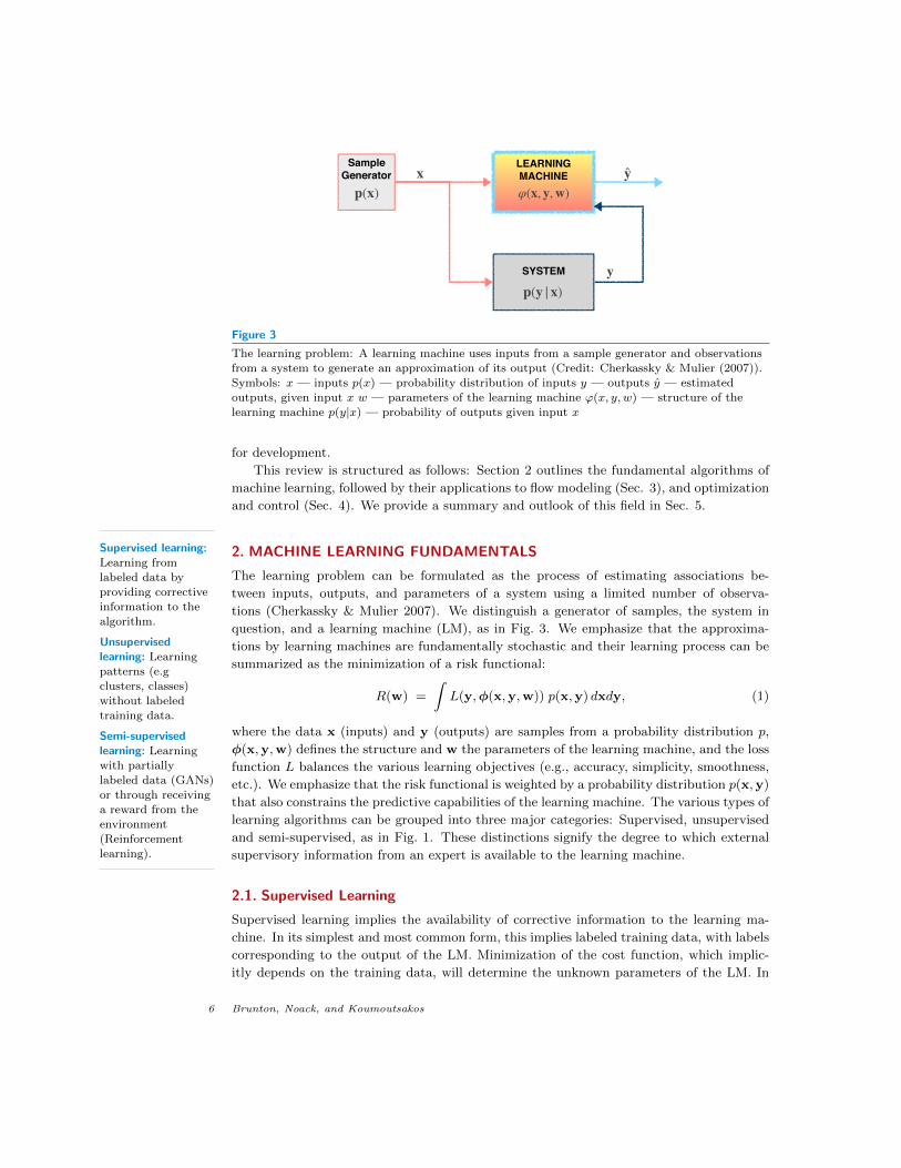
Figure 3

The learning problem: A learning machine uses inputs from a sample generator and observations

from a system to generate an approximation of its output (Credit: Cherkassky & Mulier (2007)).Symbols: x — inputs p(x) — probability distribution of inputs y — outputs y — estimated

outputs, given input x w — parameters of the learning machine ϕ(x, y, w) — structure of the

learning machine p(y|x) — probability of outputs given input x

for development.

This review is structured as follows: Section 2 outlines the fundamental algorithms of

machine learning, followed by their applications to flow modeling (Sec. 3), and optimization

and control (Sec. 4). We provide a summary and outlook of this field in Sec. 5.

2. MACHINE LEARNING FUNDAMENTALS

The learning problem can be formulated as the process of estimating associations be-

tween inputs, outputs, and parameters of a system using a limited number of observa-

tions (Cherkassky & Mulier 2007). We distinguish a generator of samples, the system in

question, and a learning machine (LM), as in Fig. 3. We emphasize that the approxima-

tions by learning machines are fundamentally stochastic and their learning process can be

summarized as the minimization of a risk functional:

R(w) =

∫L(y,φ(x,y,w)) p(x,y) dxdy, (1)

where the data x (inputs) and y (outputs) are samples from a probability distribution p,

φ(x,y,w) defines the structure and w the parameters of the learning machine, and the loss

function L balances the various learning objectives (e.g., accuracy, simplicity, smoothness,

etc.). We emphasize that the risk functional is weighted by a probability distribution p(x,y)

that also constrains the predictive capabilities of the learning machine. The various types of

learning algorithms can be grouped into three major categories: Supervised, unsupervised

and semi-supervised, as in Fig. 1. These distinctions signify the degree to which external

supervisory information from an expert is available to the learning machine.

Supervised learning:Learning from

labeled data by

providing correctiveinformation to the

algorithm.

Unsupervisedlearning: Learning

patterns (e.g

clusters, classes)without labeled

training data.

Semi-supervisedlearning: Learning

with partially

labeled data (GANs)or through receiving

a reward from theenvironment

(Reinforcementlearning).

2.1. Supervised Learning

Supervised learning implies the availability of corrective information to the learning ma-

chine. In its simplest and most common form, this implies labeled training data, with labels

corresponding to the output of the LM. Minimization of the cost function, which implic-

itly depends on the training data, will determine the unknown parameters of the LM. In


xt+1

ht+1

LSTM

xt�1

ht+1

LSTM

xt

ht�1�

ht

ht

ct�1 ct�

�

+tanh

�tanh

�

�

xt+1

ht+1

RNN

xt�1

ht�1

RNN

xt

tanh

ht�1 ht

ht

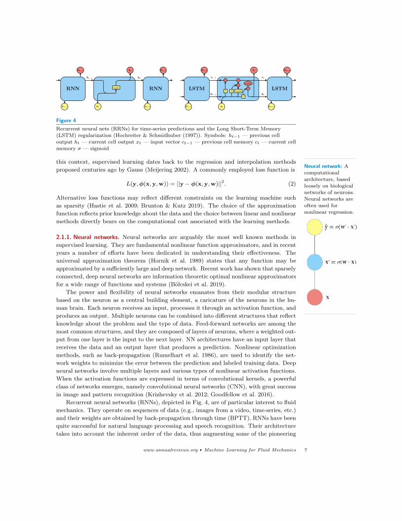
Figure 4

Recurrent neural nets (RRNs) for time-series predictions and the Long Short-Term Memory

(LSTM) regularization (Hochreiter & Schmidhuber (1997)). Symbols: ht−1 — previous cell

output ht — current cell output xt — input vector ct−1 — previous cell memory ct — current cellmemory σ — sigmoid

this context, supervised learning dates back to the regression and interpolation methods

proposed centuries ago by Gauss (Meijering 2002). A commonly employed loss function is

L(y,φ(x,y,w)) = ||y − φ(x,y,w)||2. (2)

Alternative loss functions may reflect different constraints on the learning machine such

as sparsity (Hastie et al. 2009; Brunton & Kutz 2019). The choice of the approximation

function reflects prior knowledge about the data and the choice between linear and nonlinear

methods directly bears on the computational cost associated with the learning methods.

2.1.1. Neural networks. Neural networks are arguably the most well known methods in

supervised learning. They are fundamental nonlinear function approximators, and in recent

years a number of efforts have been dedicated in understanding their effectiveness. The

universal approximation theorem (Hornik et al. 1989) states that any function may be

approximated by a sufficiently large and deep network. Recent work has shown that sparsely

connected, deep neural networks are information theoretic optimal nonlinear approximators

for a wide range of functions and systems (Bolcskei et al. 2019).

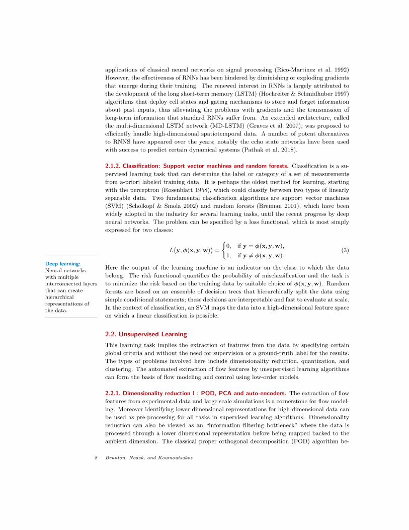
Neural network: Acomputational

architecture, based

loosely on biologicalnetworks of neurons.

Neural networks areoften used for

nonlinear regression.

The power and flexibility of neural networks emanates from their modular structure

based on the neuron as a central building element, a caricature of the neurons in the hu-

man brain. Each neuron receives an input, processes it through an activation function, and

produces an output. Multiple neurons can be combined into different structures that reflect

knowledge about the problem and the type of data. Feed-forward networks are among the

most common structures, and they are composed of layers of neurons, where a weighted out-

put from one layer is the input to the next layer. NN architectures have an input layer that

receives the data and an output layer that produces a prediction. Nonlinear optimization

methods, such as back-propagation (Rumelhart et al. 1986), are used to identify the net-

work weights to minimize the error between the prediction and labeled training data. Deep

neural networks involve multiple layers and various types of nonlinear activation functions.

When the activation functions are expressed in terms of convolutional kernels, a powerful

class of networks emerges, namely convolutional neural networks (CNN), with great success

in image and pattern recognition (Krizhevsky et al. 2012; Goodfellow et al. 2016).

Recurrent neural networks (RNNs), depicted in Fig. 4, are of particular interest to fluid

mechanics. They operate on sequences of data (e.g., images from a video, time-series, etc.)

and their weights are obtained by back-propagation through time (BPTT). RNNs have been

quite successful for natural language processing and speech recognition. Their architecture

takes into account the inherent order of the data, thus augmenting some of the pioneering


applications of classical neural networks on signal processing (Rico-Martinez et al. 1992)

However, the effectiveness of RNNs has been hindered by diminishing or exploding gradients

that emerge during their training. The renewed interest in RNNs is largely attributed to

the development of the long short-term memory (LSTM) (Hochreiter & Schmidhuber 1997)

algorithms that deploy cell states and gating mechanisms to store and forget information

about past inputs, thus alleviating the problems with gradients and the transmission of

long-term information that standard RNNs suffer from. An extended architecture, called

the multi-dimensional LSTM network (MD-LSTM) (Graves et al. 2007), was proposed to

efficiently handle high-dimensional spatiotemporal data. A number of potent alternatives

to RNNS have appeared over the years; notably the echo state networks have been used

with success to predict certain dynamical systems (Pathak et al. 2018).

2.1.2. Classification: Support vector machines and random forests. Classification is a su-

pervised learning task that can determine the label or category of a set of measurements

from a-priori labeled training data. It is perhaps the oldest method for learning, starting

with the perceptron (Rosenblatt 1958), which could classify between two types of linearly

separable data. Two fundamental classification algorithms are support vector machines

(SVM) (Scholkopf & Smola 2002) and random forests (Breiman 2001), which have been

widely adopted in the industry for several learning tasks, until the recent progress by deep

neural networks. The problem can be specified by a loss functional, which is most simply

expressed for two classes:

L(y,φ(x,y,w)

)=

{0, if y = φ(x,y,w),

1, if y 6= φ(x,y,w).(3)

Here the output of the learning machine is an indicator on the class to which the data

belong. The risk functional quantifies the probability of misclassification and the task is

to minimize the risk based on the training data by suitable choice of φ(x,y,w). Random

forests are based on an ensemble of decision trees that hierarchically split the data using

simple conditional statements; these decisions are interpretable and fast to evaluate at scale.

In the context of classification, an SVM maps the data into a high-dimensional feature space

on which a linear classification is possible.

Deep learning:Neural networks

with multipleinterconnected layers

that can create

hierarchicalrepresentations of

the data.

2.2. Unsupervised Learning

This learning task implies the extraction of features from the data by specifying certain

global criteria and without the need for supervision or a ground-truth label for the results.

The types of problems involved here include dimensionality reduction, quantization, and

clustering. The automated extraction of flow features by unsupervised learning algorithms

can form the basis of flow modeling and control using low-order models.

2.2.1. Dimensionality reduction I : POD, PCA and auto-encoders. The extraction of flow

features from experimental data and large scale simulations is a cornerstone for flow model-

ing. Moreover identifying lower dimensional representations for high-dimensional data can

be used as pre-processing for all tasks in supervised learning algorithms. Dimensionality

reduction can also be viewed as an “information filtering bottleneck” where the data is

processed through a lower dimensional representation before being mapped backed to the

ambient dimension. The classical proper orthogonal decomposition (POD) algorithm be-


retain M < D eigenvectors

x = 1N

N

∑n = 1

xn

S = 1N

N

∑n = 1

(xn − x)(xn − x)T

Sui = λiui

x W ⋅ x = z

WT ⋅ z = x

x

retain M < D eigenvectors

x = 1N

N

∑n = 1

xn

S = 1N

N

∑n = 1

(xn − x)(xn − x)T

Sui = λiui

x x x x

z z

ϕ(x) ψ(z)U V

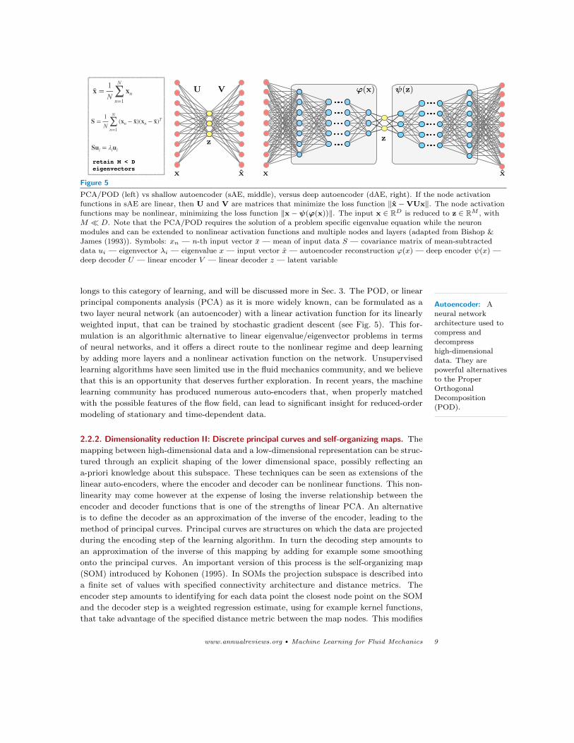
Figure 5

PCA/POD (left) vs shallow autoencoder (sAE, middle), versus deep autoencoder (dAE, right). If the node activationfunctions in sAE are linear, then U and V are matrices that minimize the loss function ‖x−VUx‖. The node activation

functions may be nonlinear, minimizing the loss function ‖x−ψ(ϕ(x))‖. The input x ∈ RD is reduced to z ∈ RM , with

M � D. Note that the PCA/POD requires the solution of a problem specific eigenvalue equation while the neuronmodules and can be extended to nonlinear activation functions and multiple nodes and layers (adapted from Bishop &

James (1993)). Symbols: xn — n-th input vector x — mean of input data S — covariance matrix of mean-subtracteddata ui — eigenvector λi — eigenvalue x — input vector x — autoencoder reconstruction ϕ(x) — deep encoder ψ(x) —

deep decoder U — linear encoder V — linear decoder z — latent variable

longs to this category of learning, and will be discussed more in Sec. 3. The POD, or linear

principal components analysis (PCA) as it is more widely known, can be formulated as a

two layer neural network (an autoencoder) with a linear activation function for its linearly

weighted input, that can be trained by stochastic gradient descent (see Fig. 5). This for-

mulation is an algorithmic alternative to linear eigenvalue/eigenvector problems in terms

of neural networks, and it offers a direct route to the nonlinear regime and deep learning

by adding more layers and a nonlinear activation function on the network. Unsupervised

learning algorithms have seen limited use in the fluid mechanics community, and we believe

that this is an opportunity that deserves further exploration. In recent years, the machine

learning community has produced numerous auto-encoders that, when properly matched

with the possible features of the flow field, can lead to significant insight for reduced-order

modeling of stationary and time-dependent data.

Autoencoder: A

neural networkarchitecture used to

compress and

decompresshigh-dimensional

data. They are

powerful alternativesto the Proper

Orthogonal

Decomposition(POD).

2.2.2. Dimensionality reduction II: Discrete principal curves and self-organizing maps. The

mapping between high-dimensional data and a low-dimensional representation can be struc-

tured through an explicit shaping of the lower dimensional space, possibly reflecting an

a-priori knowledge about this subspace. These techniques can be seen as extensions of the

linear auto-encoders, where the encoder and decoder can be nonlinear functions. This non-

linearity may come however at the expense of losing the inverse relationship between the

encoder and decoder functions that is one of the strengths of linear PCA. An alternative

is to define the decoder as an approximation of the inverse of the encoder, leading to the

method of principal curves. Principal curves are structures on which the data are projected

during the encoding step of the learning algorithm. In turn the decoding step amounts to

an approximation of the inverse of this mapping by adding for example some smoothing

onto the principal curves. An important version of this process is the self-organizing map

(SOM) introduced by Kohonen (1995). In SOMs the projection subspace is described into

a finite set of values with specified connectivity architecture and distance metrics. The

encoder step amounts to identifying for each data point the closest node point on the SOM

and the decoder step is a weighted regression estimate, using for example kernel functions,

that take advantage of the specified distance metric between the map nodes. This modifies


the node centers, and the process can be iterated until the empirical risk of the autoencoder

has been minimized. The SOM capabilities can be exemplified by comparing it to linear

PCA for two dimensional set of points. The linear PCA will provide as an approximation

the least squares straight line between the points whereas the SOM will map the points

onto a curved line that better approximates the data. We note that SOMs can be extended

to areas beyond floating point data and they offer an interesting way for creating data bases

based on features of flow fields.

2.2.3. Clustering and vector quantization. Clustering is an unsupervised learning technique

that identifies similar groups in the data. The most common algorithm is k-means cluster-

ing, which partitions data into k clusters; an observation belongs to the cluster with the

nearest centroid, resulting in a partition of data space into Voronoi cells.

Vector quantizers identify representative points for data that can be partitioned into a

predetermined number of clusters. These points can then be used instead of the full data

set so that future samples can be approximated by them. The vector quantizer φ(x,w

)provides a mapping between the data x and the coordinates of the cluster centers. The loss

function is usually the squared distortion of the data from the cluster centers, which must

be minimized to identify the parameters of the quantizer:

L(φ(x,w)) = ||x− φ(x,w)||2. (4)

We note that vector quantization is a data reduction method, not necessarily employed for

dimensionality reduction. In the latter the learning problem seeks to identify low dimen-

sional features in high dimensional data, whereas quantization amounts to finding represen-

tative clusters of the data. Vector quantization must also be distinguished from clustering

as in the former the number of desired centers is determined a-priori whereas clustering

aims to identify meaningful groupings in the data. When these groupings are represented

by some prototypes then clustering and quantization have strong similarities.

2.3. Semi-Supervised Learning

Semi-supervised learning algorithms operate under partial supervision, either with limited

labeled training data, or with other corrective information from the environment. Two

algorithms in this category are generative adversarial networks (GAN) and reinforcement

learning (RL). In both cases the learning machine is (self-)trained through a game like

process as discussed below.

2.3.1. Generative adversarial networks (GAN). GANs are learning algorithms that result in

a generative model, i.e. a model that produces data according to a probability distribution,

which mimics that of the data used for its training. The learning machine is composed

of two networks that compete with each other in a zero sum game (Goodfellow et al.

2014). The generative network produces candidate data examples that are evaluated by the

discriminative, or critic, network to optimize a certain task. The generative (G) network’s

training objective is to synthesize novel examples of data to fool the discriminative network

into misclassifying them as belonging to the true data distribution. The weights of these

networks (N) are obtained through a process, inspired by game theory, called adversarial (A)

learning. The final objective of the GAN training process is to identify the generative model

that produces an output that reflects the underlying system. Labeled data are provided


by the discriminator network and the function to be minimized is the Kullback-Leibler

divergence between the two distributions. In the ensuing “game”, the discriminator aims

to maximize the probability of it discriminating between true data and data produced by

the generator, while the generator aims to minimize the same probability. Because the

generative and discriminative networks essentially train themselves, after initialization with

labeled training data, this procedure is often referred to as self-supervised. This self-training

process adds to the appeal of GANs but at the same time one must be cautious on whether

an equilibrium will ever be reached in the above mentioned game. As with other training

algorithms, large amounts of data help the process but, at the moment, there is no guarantee

of convergence.

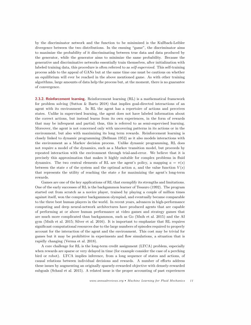
2.3.2. Reinforcement learning. Reinforcement learning (RL) is a mathematical framework

for problem solving (Sutton & Barto 2018) that implies goal-directed interactions of an

agent with its environment. In RL the agent has a repertoire of actions and perceives

states. Unlike in supervised learning, the agent does not have labeled information about

the correct actions, but instead learns from its own experiences, in the form of rewards

that may be infrequent and partial; thus, this is referred to as semi-supervised learning.

Moreover, the agent is not concerned only with uncovering patterns in its actions or in the

environment, but also with maximizing its long term rewards. Reinforcement learning is

closely linked to dynamic programming (Bellman 1952) as it also models interactions with

the environment as a Markov decision process. Unlike dynamic programming, RL does

not require a model of the dynamics, such as a Markov transition model, but proceeds by

repeated interaction with the environment through trial-and-error. We believe that it is

precisely this approximation that makes it highly suitable for complex problems in fluid

dynamics. The two central elements of RL are the agent’s policy, a mapping a = π(s)

between the state s of the system and the optimal action a, and the value function V (s)

that represents the utility of reaching the state s for maximizing the agent’s long-term

rewards.

Games are one of the key applications of RL that exemplify its strengths and limitations.

One of the early successes of RL is the backgammon learner of Tesauro (1992). The program

started out from scratch as a novice player, trained by playing a couple of million times

against itself, won the computer backgammon olympiad, and eventually became comparable

to the three best human players in the world. In recent years, advances in high-performance

computing and deep neural-network architectures have produced agents that are capable

of performing at or above human performance at video games and strategy games that

are much more complicated than backgammon, such as Go (Mnih et al. 2015) and the AI

gym (Mnih et al. 2015; Silver et al. 2016). It is important to emphasize that RL requires

significant computational resources due to the large numbers of episodes required to properly

account for the interaction of the agent and the environment. This cost may be trivial for

games but it may be prohibitive in experiments and flow simulations, a situation that is

rapidly changing (Verma et al. 2018).

A core challenge for RL is the long-term credit assignment (LTCA) problem, especially

when rewards are sparse or very delayed in time (for example consider the case of a perching

bird or robot). LTCA implies inference, from a long sequence of states and actions, of

causal relations between individual decisions and rewards. A number of efforts address

these issues by augmenting an originally sparsely-rewarded objective with densely-rewarded

subgoals (Schaul et al. 2015). A related issue is the proper accounting of past experiences


by the agent as it actively forms a new policy Novati et al. (2019).

2.4. Stochastic Optimization: A Learning Algorithms Perspective

Optimization is an inherent part of learning, as a risk functional is minimized in order

to identify the parameters of the learning machine. There is, however, one more link

that we wish to highlight in this review: optimization (and search) algorithms can be

cast in the context of learning algorithms and more specifically as the process of learning

the probability distribution of the design points that maximize a certain objective. This

connection was pioneered by Rechenberg (1973); Schwefel (1977), who introduced Evolution

Strategies (ES) and adapted the variance of their search space based on the success rate

of their experiments. This process is also reminiscent of the operations of selection and

mutation that are key ingredients of Genetic Algorithms (GA) (Holland 1975) and Genetic

Programming (Koza 1992). ES and GAs algorithms can be considered as hybrids between

gradient search strategies, which may effectively march downhill towards a minimum, and

Latin-Hypercube or Monte-Carlo sampling methods, which maximally explore the search

space. Genetic programming was developed in the late 1980s by J. R. Koza, a PhD student

of John Holland. Genetic programming generalized parameter optimization to function

optimization, initially coded as a tree of operations (Koza 1992). A critical aspect of these

algorithms is that they rely on an iterative construction of the probability distribution,

based on data values of the objective function. This iterative construction can be lenhthy

and practically impossible for problems with expensive objective function evaluations.

Over the past twenty years, ES and GAs have begun to converge into the framework of

estimation of distribution algorithms (EDAs). The CMA-ES algorithm (Ostermeier et al.

1994; Hansen et al. 2003) is a prominent example of evolution strategies using an adaptive

estimation of the covariance matrix of a Gaussian probability distribution, to guide the

search for optimal parameters. This covariance matrix is adapted iteratively using the best

points in each iteration. The CMA-ES is closely related to a number of other algorithms

including the mixed Bayesian optimization algorithms (MBOAs) (Pelikan et al. 2004), and

the reader is referred to Kern et al. (2004) for a comparative review. In recent years,

this line of work has evolved into the more generalized information-geometric optimization

(IGO) framework (Ollivier et al. 2017). IGO algorithms allow for families of probability

distributions whose parameters are learned during the optimization process and maintain

the cost function invariance as a major design principle. The resulting algorithm makes

no assumption on the objective function to be optimized and its flow is equivalent to a

stochastic gradient descent. These techniques have been proven to be effective on a number

of simplified benchmark problems; however, their scaling remains unclear and there are

few guarantees for convergence in cost function landscapes such as those encountered in

complex fluid dynamics problems. We note also that there is interest in deploying these

methods in order to minimize the cost functions associated with classical machine learning

tasks (Salimans et al. 2017).

2.5. Important Topics We Have Not Covered: Bayesian Inference, GaussianProcesses

There are a number of learning algorithms that this review does not address, but which

demand particular attention from the fluid mechanics community. First and foremost we

wish to mention Bayesian inference, which aims to inform the model structure and its pa-


rameters from data in a probabilistic framework. Bayesian inference is fundamental for

uncertainty quantification, and it is also fundamentally a learning method, as data are

used to adapt the model estimates. An alternative view casts machine learning algorithms

in a Bayesian framework (Theodoridis 2015; Barber 2012). The above mentioned opti-

mization algorithms provide also a link between these two views. Whereas optimization

algorithms aim to provide the best parameters of a model for given data in a stochastic

manner, Bayesian inference aims to provide the full probability distribution of the model

parameters. It may be argued that Bayesian inference is an even more powerful language

than machine learning, as it provides probability distributions for all parameters, leading to

robust predictions, rather than single values, as is usually the case with classical machine

learning algorithms. However, a key drawback for Bayesian inference is its computational

cost, as it involves sampling and integration in high-dimensional spaces, which can be pro-

hibitive for expensive function evaluations (e.g. wind tunnel experiments or large scale

DNS). Along the same lines one must mention Gaussian processes (GaP), which resemble

kernel-based methods for regression. However, GaPs develop these kernels adaptively based

on the available data. They also provide probability distributions for the respective model

parameters. GaPs have been used extensively in problems related to time-dependent prob-

lems and they may be considered competitors, albeit more costly, to RNNs and echo state

networks. Finally, we note the use of GaPs as surrogates for expensive cost

3. FLOW MODELING WITH MACHINE LEARNING

First principles, such as conservation laws, have been the dominant building blocks for flow

modeling over the past centuries. However, for high Reynolds numbers, scale resolving sim-

ulations using the most prominent model in fluid mechanics, the Navier-Stokes equations,

is beyond our current computational resources. An alternative is to perform simulations

based on approximations of these equations or laboratory experiments for a specific configu-

ration. However, simulations and experiments are expensive for iterative optimization, and

simulations are often too slow for real-time control (Brunton & Noack 2015). Consequently,

considerable effort has been placed on obtaining accurate and efficient reduced-order mod-

els that capture essential flow mechanisms at a fraction of the cost (Rowley & Dawson

2016). Machine learning presents new avenues for dimensionality reduction and reduced

order modeling in fluid mechanics by providing a concise framework that complements and

extends existing methodologies.

Reduced-orderModel (ROM):Representation of a

high-dimensionalsystem in terms of a

low-dimensional one,

balancing accuracyand efficiency.

We distinguish two complementary directions: dimensionality reduction and reduced-

order modeling. Dimensionality reduction involves extracting key features and dominant

patterns that may be used as reduced coordinates where the fluid is compactly and effi-

ciently described (Taira et al. 2017). Reduced-order modeling describes the spatiotemporal

evolution of the flow as a parametrized dynamical system, although it may also involve

developing a statistical map from parameters to averaged quantities, such as drag.

There have been significant efforts to identify coordinate transformations and reductions

that simplify dynamics and capture essential flow physics: the proper orthogonal decom-

position (POD) is a notable example (Lumley 1970). Model reduction, such as Galerkin

projection of the Navier-Stokes equations onto an orthogonal basis of POD modes, benefits

from a close connection to the governing equations; however, it is intrusive, requiring hu-

man expertise to develop models from a working simulation. Machine learning constitutes

a rapidly growing body of modular algorithms for data-driven system identification and


modeling. Unique aspects of data-driven modeling of fluid flows include the availability of

partial prior knowledge of the governing equations, constraints, and symmetries. With ad-

vances in simulation capabilities and experimental techniques, fluid dynamics is becoming

a data rich field, thus amenable to a wealth of machine learning algorithms.

In this review, we distinguish machine learning algorithms to model flow 1) kinematics

through the extraction flow features and 2) dynamics through the adoption of various

learning architectures.

3.1. Flow Feature Extraction

Pattern recognition and data mining are core strengths of machine learning with many

techniques that are readily applicable to spatiotemporal flow data. We distinguish linear

and nonlinear dimensionality reduction techniques, followed by clustering and classification.

We also consider accelerated measurement and computation strategies, as well as methods

to process experimental flow field data.

3.1.1. Dimensionality reduction: Linear and nonlinear embeddings. A common approach

in fluid dynamics simulation and modeling is to define an orthogonal linear transformation

from physical coordinates into a modal basis. The POD provides such an orthogonal basis

for complex geometries based on empirical measurements. Sirovich (1987) introduced the

snapshot POD, which reduces the computation to a simple data-driven procedure involving

a singular value decomposition. Interestingly, in the same year, Sirovich used POD to

generate a low-dimensional feature space for the classification of human faces, which is a

foundation for much of modern computer vision (Sirovich & Kirby 1987).

POD is closely related to the algorithm of principal component analysis (PCA), one

of the fundamental algorithms of applied statistics and machine learning, to describe cor-

relations in high-dimensional data. We recall that the PCA can be expressed as a two

layer neural network, called an autoencoder, to compress high-dimensional data for a com-

pact representation as shown in Fig. 5. This network embeds high-dimensional data into a

low-dimensional latent space, and then decodes from the latent space back to the original

high-dimensional space. When the network nodes are linear and the encoder and decoder

are constrained to be transposes of one another, the autoencoder is closely related to the

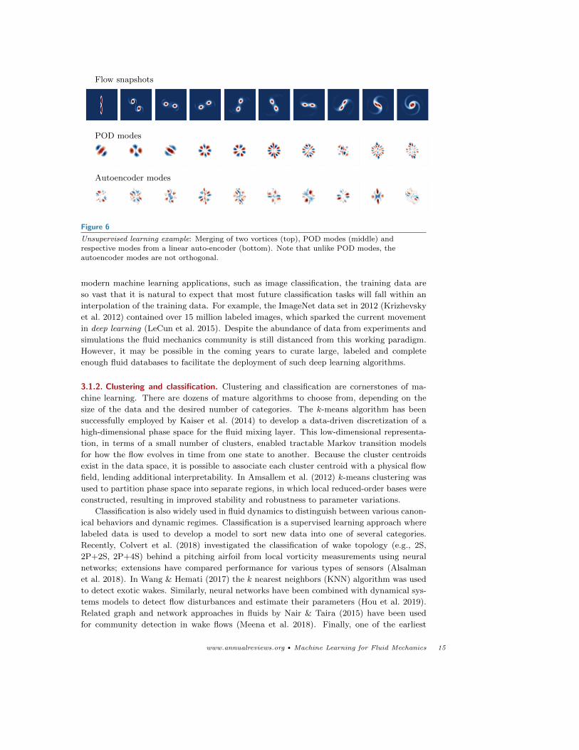
standard POD/PCA decomposition ( (Baldi & Hornik 1989), please see also Fig. 6). How-

ever, the structure of the neural network autoencoder is modular, and by using nonlinear

activation units for the nodes, it is possible to develop nonlinear embeddings, potentially

providing more compact coordinates. This observation led to the development of one of

the first applications of deep neural networks to reconstruct the near wall velocity field

in a turbulent channel flow using wall pressure and shear (Milano & Koumoutsakos 2002).

More powerful autoencoders are today available in the ML community and this link deserves

further exploration.

On the basis of the universal approximation theorem (Hornik et al. 1989), stating that a

sufficiently large neural network can represent an arbitrarily complex input–output function,

deep neural networks are increasingly used to obtain more effective nonlinear coordinates

for complex flows. However, deep learning often implies the availability of large volumes

of training data that far exceed the parameters of the network. The resulting models are

usually good for interpolation but may not be suitable for extrapolation when the new input

data have different probability distributions than the training data (see Eq. (1)). In many


Flow snapshots

POD modes

Autoencoder modes

Figure 6

Unsupervised learning example: Merging of two vortices (top), POD modes (middle) and

respective modes from a linear auto-encoder (bottom). Note that unlike POD modes, theautoencoder modes are not orthogonal.

modern machine learning applications, such as image classification, the training data are

so vast that it is natural to expect that most future classification tasks will fall within an

interpolation of the training data. For example, the ImageNet data set in 2012 (Krizhevsky

et al. 2012) contained over 15 million labeled images, which sparked the current movement

in deep learning (LeCun et al. 2015). Despite the abundance of data from experiments and

simulations the fluid mechanics community is still distanced from this working paradigm.

However, it may be possible in the coming years to curate large, labeled and complete

enough fluid databases to facilitate the deployment of such deep learning algorithms.

3.1.2. Clustering and classification. Clustering and classification are cornerstones of ma-

chine learning. There are dozens of mature algorithms to choose from, depending on the

size of the data and the desired number of categories. The k-means algorithm has been

successfully employed by Kaiser et al. (2014) to develop a data-driven discretization of a

high-dimensional phase space for the fluid mixing layer. This low-dimensional representa-

tion, in terms of a small number of clusters, enabled tractable Markov transition models

for how the flow evolves in time from one state to another. Because the cluster centroids

exist in the data space, it is possible to associate each cluster centroid with a physical flow

field, lending additional interpretability. In Amsallem et al. (2012) k-means clustering was

used to partition phase space into separate regions, in which local reduced-order bases were

constructed, resulting in improved stability and robustness to parameter variations.

Classification is also widely used in fluid dynamics to distinguish between various canon-

ical behaviors and dynamic regimes. Classification is a supervised learning approach where

labeled data is used to develop a model to sort new data into one of several categories.

Recently, Colvert et al. (2018) investigated the classification of wake topology (e.g., 2S,

2P+2S, 2P+4S) behind a pitching airfoil from local vorticity measurements using neural

networks; extensions have compared performance for various types of sensors (Alsalman

et al. 2018). In Wang & Hemati (2017) the k nearest neighbors (KNN) algorithm was used

to detect exotic wakes. Similarly, neural networks have been combined with dynamical sys-

tems models to detect flow disturbances and estimate their parameters (Hou et al. 2019).

Related graph and network approaches in fluids by Nair & Taira (2015) have been used

for community detection in wake flows (Meena et al. 2018). Finally, one of the earliest


examples of machine learning classification in fluid dynamics by Bright et al. (2013) was

based on sparse representation (Wright et al. 2009).

3.1.3. Sparse and randomized methods. In parallel to machine learning, there have been

great strides in sparse optimization and randomized linear algebra. Machine learning and

sparse algorithms are synergistic, in that underlying low-dimensional representations facili-

tate sparse measurements (Manohar et al. 2018) and fast randomized computations (Halko

et al. 2011). Decreasing the amount of data to train and execute a model is important

when a fast decision is required, as in control. In this context algorithms for the efficient

acquisition and reconstruction of sparse signals, such as compressed sensing Donoho (2006),

have already been leveraged for compact representations of wall-bounded turbulence (Bour-

guignon et al. 2014) and for POD based flow reconstruction (Bai et al. 2014).

Low-dimensional structure in data also facilitates dramatically accelerated computations

via randomized linear algebra (Mahoney 2011; Halko et al. 2011). If a matrix has low-rank

structure, then there are extremely efficient matrix decomposition algorithms based on

random sampling; this is closely related to the idea of sparsity and the high-dimensional

geometry of sparse vectors. The basic idea is that if a large matrix has low-dimensional

structure, then with high probability this structure will be preserved after projecting the

columns or rows onto a random low-dimensional subspace, facilitating efficient downstream

computations. These so-called randomized numerical methods have the potential to trans-

form computational linear algebra, providing accurate matrix decompositions at a fraction

of the cost of deterministic methods. For example, randomized linear algebra may be

used to efficiently compute the singular value decomposition, which is used to compute

PCA (Rokhlin et al. 2009; Halko et al. 2011).

3.1.4. Super resolution and flow cleansing. Much of machine learning is focused on imaging

science, providing robust approaches to improve resolution and remove noise and corruption

based on statistical inference. These super resolution and de-noising algorithms have the

potential to improve the quality of both simulations and experiments in fluids.

Super resolution involves the inference of a high-resolution image from low-resolution

measurements, leveraging the statistical structure of high-resolution training data. Several

approaches have been developed for super resolution, for example based on a library of

examples (Freeman et al. 2002), sparse representation in a library (Yang et al. 2010), and

most recently based on convolutional neural networks (Dong et al. 2014). Experimental flow

field measurements from particle image velocimetry (PIV) (Willert & Gharib 1991; Adrian

1991) provide a compelling application where there is a tension between local flow resolution

and the size of the imaging domain. Super resolution could leverage expensive and high-

resolution data on smaller domains to improve the resolution on a larger imaging domain.

Large eddy simulations (LES) (Germano et al. 1991; Meneveau & Katz 2000) may also

benefit from super resolution to infer the high-resolution structure inside a low-resolution

cell that is required to compute boundary conditions. Recently Fukami et al. (2018) have

developed a CNN-based super-resolution algorithm and demonstrated its effectiveness on

turbulent flow reconstruction, showing that the energy spectrum is accurately preserved.

One drawback of super-resolution is that it is often extremely costly computationally, mak-

ing it useful for applications where high-resolution imaging may be prohibitively expensive;

however, improved neural-network based approaches may drive the cost down significantly.

We note also that Xie et al. (2018) recently employed GANs for super-resolution.


The processing of experimental PIV and particle tracking has been also one of the first

applications of machine learning. Neural networks have been used for fast PIV (Knaak et al.

1997) and particle tracking velocimetry (Labonte 1999), with impressive demonstrations for

three-dimensional Lagrangian particle tracking (Ouellette et al. 2006). More recently, deep

convolutional neural networks have been used to construct velocity fields from PIV image

pairs (Lee et al. 2017). Related approaches have also been used to detect spurious vectors

in PIV data (Liang et al. 2003) to remove outliers and fill in corrupt pixels.

3.2. Modeling Flow Dynamics

A central goal of modeling is to balance efficiency and accuracy. When modeling physical

systems, interpretability and generalizability are also critical considerations.

3.2.1. Linear models through nonlinear embeddings: DMD and Koopman analysis. Many

classical techniques in system identification may be considered machine learning, as they

are data-driven models that generalize beyond the training data. The dynamic mode de-

composition (DMD) (Schmid 2010; Kutz et al. 2016) is a modern approach, to extract

spatiotemporal coherent structures from time-series data of fluid flows, resulting in a low-

dimensional linear model for the evolution of these dominant coherent structures. DMD is

based on data-driven regression and is equally valid for time-resolved experimental and nu-

merical data. DMD is closely related to the Koopman operator (Rowley et al. 2009; Mezic

2013), which is an infinite dimensional linear operator that describes how all measurement

functions of the system evolve in time. Because the DMD algorithm is based on linear flow

field measurements (i.e., direct measurements of the fluid velocity or vorticity field), the

resulting models may not be able to capture nonlinear transients.

Recently, there has been a concerted effort to identify nonlinear measurements that

evolve linearly in time, establishing a coordinate system where the nonlinear dynamics

appear linear. The extended DMD (Williams et al. 2015) and variational approach of

conformation dynamics (VAC) (Noe & Nuske 2013; Nuske et al. 2016) enrich the model with

nonlinear measurements, leveraging kernel methods (Williams et al. 2015) and dictionary

learning (Li et al. 2017). These special nonlinear measurements are generally challenging

to represent, and deep learning architectures are now used to identify nonlinear Koopman

coordinate systems where the dynamics appear linear (Wehmeyer & Noe 2018; Mardt et al.

2018; Takeishi et al. 2017; Lusch et al. 2018). The VAMPnet architecture (Wehmeyer &

Noe 2018; Mardt et al. 2018) uses a time-lagged auto-encoder and a custom variational

score to identify Koopman coordinates on an impressive protein folding example. Based

on the performance of VAMPnet, fluid dynamics may benefit from neighboring fields, such

as molecular dynamics, which have similar modeling issues, including stochasticity, coarse-

grained dynamics, and massive separation of time scales.

3.2.2. Neural network modeling. Over the last three decades neural networks have been

used to model dynamical systems and fluid mechanics problems. Early examples include

the use of NNs to learn the solutions of ordinary and partial differential equations (Dis-

sanayake & Phan-Thien 1994; Gonzalez-Garcia et al. 1998; Lagaris et al. 1998). We note

that the potential of this work has not been fully explored and in recent years there is

further advances (Chen et al. 2018; Raissi & Karniadakis 2018) including discrete and con-

tinuous in time networks. We note also the possibility of using these methods to uncover


latent variables and reduce the number of parametric studies often associated with partial

differential equations Raissi et al. (2019). Neural networks are also frequently employed

in nonlinear system identification techniques, such as NARMAX, which are often used to

model fluid systems (Glaz et al. 2010). In fluid mechanics, neural networks were widely

used to model heat transfer (Jambunathan et al. 1996), turbomachinery (Pierret & Van den

Braembussche 1998), turbulent flows (Milano & Koumoutsakos 2002), and other problems

in aeronautics (Faller & Schreck 1996).

Recurrent Neural Netwosk with LSTMs (Hochreiter & Schmidhuber (1997) have been

revolutionary for speech recognition, and they are considered one of the landmark successes

of artificial intellignece. The are currently being used to model dynamical systems and

for data driven predictions of extreme events (Wan et al. 2018; Vlachas et al. 2018). An

interesting finding of these studies is that combining data driven and reduced order mod-

els is a potent method that outperforms each of its components on a number of studies.

Generative adversarial networks (GANs) (Goodfellow et al. 2014) are also being used to

infer dynamical systems from data (Wu et al. 2018). GANs have potential to aid in the

modeling and simulation of turbulence (Kim et al. 2018), although this field is nascent, yet

well worthy of exploration.

Despite the promise and widespread use of neural networks in dynamical systems, a

number of challenges remains. Neural networks are fundamentally interpolative, and so the

function is only well approximated in the span (or under the probability distribution) of

the sampled data used to train them. Thus, caution should be exercised when using neural

network models for an extrapolation task. In many computer vision and speech recognition

examples, the training data are so vast that nearly all future tasks may be viewed as an

interpolation on the training data. However, this scale of training has not been achieve

to date in fluid mechanics. Similarly, neural network models are prone to overfitting, and

care must be taken to cross-validate models on a sufficiently chosen test set; best practices

are discussed in Goodfellow et al. (2016). Finally, it is important to explicitly incorporate

physical properties such as symmetries, constraints, and conserved quantities.

3.2.3. Parsimonious nonlinear models. Parsimony is a recurring theme in mathematical

physics, from Hamilton’s principle of least action to the apparent simplicity of many gov-

erning equations. In contrast to the raw representational power of neural networks, machine

learning algorithms are also being employed to identify minimal models that balance predic-

tive accuracy with model complexity, preventing overfitting and promoting interpretability

and generalizability. Genetic programming has been used to discover conservation laws and

governing equations (Schmidt & Lipson 2009). Sparse regression in a library of candidate

models has also been proposed to identify dynamical systems (Brunton et al. 2016) and

partial differential equations (Rudy et al. 2017; Schaeffer 2017). Loiseau & Brunton (2018)

identified sparse reduced-order models of several flow systems, enforcing energy conservation

as a constraint. In both genetic programming and sparse identification, a Pareto analysis

is used to identify models that have the best tradeoff between model complexity, measured

in number of terms, and predictive accuracy. In cases where the physics is known, this

approach typically discovers the correct governing equations, providing exceptional gener-

alizability compared with other leading algorithms in machine learning.

3.2.4. Closure models with machine learning. The use of machine learning to develop tur-

bulence closures is an active area of research (Duraisamy et al. 2019). The extremely wide


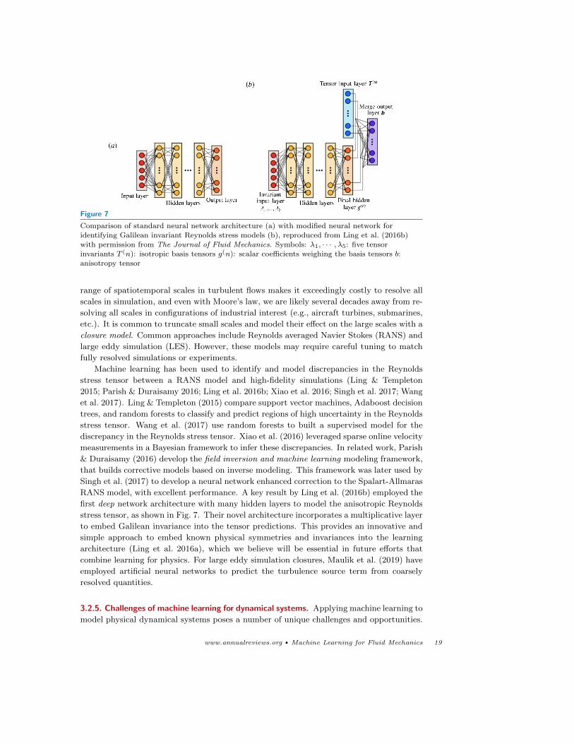
Figure 7

Comparison of standard neural network architecture (a) with modified neural network for

identifying Galilean invariant Reynolds stress models (b), reproduced from Ling et al. (2016b)

with permission from The Journal of Fluid Mechanics. Symbols: λ1, · · · , λ5: five tensorinvariants T (n): isotropic basis tensors g(n): scalar coefficients weighing the basis tensors b:

anisotropy tensor

range of spatiotemporal scales in turbulent flows makes it exceedingly costly to resolve all

scales in simulation, and even with Moore’s law, we are likely several decades away from re-

solving all scales in configurations of industrial interest (e.g., aircraft turbines, submarines,

etc.). It is common to truncate small scales and model their effect on the large scales with a

closure model. Common approaches include Reynolds averaged Navier Stokes (RANS) and

large eddy simulation (LES). However, these models may require careful tuning to match

fully resolved simulations or experiments.

Machine learning has been used to identify and model discrepancies in the Reynolds

stress tensor between a RANS model and high-fidelity simulations (Ling & Templeton

2015; Parish & Duraisamy 2016; Ling et al. 2016b; Xiao et al. 2016; Singh et al. 2017; Wang

et al. 2017). Ling & Templeton (2015) compare support vector machines, Adaboost decision

trees, and random forests to classify and predict regions of high uncertainty in the Reynolds

stress tensor. Wang et al. (2017) use random forests to built a supervised model for the

discrepancy in the Reynolds stress tensor. Xiao et al. (2016) leveraged sparse online velocity

measurements in a Bayesian framework to infer these discrepancies. In related work, Parish

& Duraisamy (2016) develop the field inversion and machine learning modeling framework,

that builds corrective models based on inverse modeling. This framework was later used by

Singh et al. (2017) to develop a neural network enhanced correction to the Spalart-Allmaras

RANS model, with excellent performance. A key result by Ling et al. (2016b) employed the

first deep network architecture with many hidden layers to model the anisotropic Reynolds

stress tensor, as shown in Fig. 7. Their novel architecture incorporates a multiplicative layer

to embed Galilean invariance into the tensor predictions. This provides an innovative and

simple approach to embed known physical symmetries and invariances into the learning

architecture (Ling et al. 2016a), which we believe will be essential in future efforts that

combine learning for physics. For large eddy simulation closures, Maulik et al. (2019) have

employed artificial neural networks to predict the turbulence source term from coarsely

resolved quantities.

3.2.5. Challenges of machine learning for dynamical systems. Applying machine learning to

model physical dynamical systems poses a number of unique challenges and opportunities.


Model interpretability and generalizability are essential cornerstones in physics. A well

crafted model will yield hypotheses for new phenomena that have not been observed before.

This principle is clearly exhibited in the parsimonious formulation of classical mechanics in

Newton’s second law.

High-dimensional systems, such as those encountered in unsteady fluid dynamics, have

the challenges of multi-scale dynamics, sensitivity to noise and disturbances, latent variables

and transients, all of which require careful attention when applying machine learning tech-

niques. In machine learning for dynamics, we distinguish two tasks: discovering unknown

physics and improving models by incorporating known physics. Many learning architec-

tures, cannot readily incorporate physical constraints in the form of symmetries, boundary

conditions, and global conservation laws. This is a critical area for continued development

and a number of recent works have presented generalizable physics models (Battaglia et al.

2018).

4. FLOW OPTIMIZATION AND CONTROL USING MACHINE LEARNING

Learning algorithms are well suited to flow optimization and control problems involving

“black-box” or multimodal cost functions. These algorithms are iterative and often require

several orders of magnitude more cost function evaluations than gradient based algorithms

(Bewley et al. 2001). Moreover they do not offer guarantees of convergence and we suggest

that they are avoided when techniques such as adjoint methods are applicable. At the

same time, techniques such as reinforcement learning have been shown to outperform even

optimal flow control strategies (Novati et al. 2019). Indeed there are several classes of flow

control and optimization problems where learning algorithms may be the method of choice

as described below.

In contrast to flow modeling, learning algorithms for optimization and control interact

with the data sampling process in several ways. First, in line with the modeling efforts

described in earlier sections, machine learning can be applied to develop explicit surrogate

models that relate the cost function and the control/optimization parameters. Surrogate

models such as neural networks can then be amenable even to gradient based methods,

although they often get stuck in local minima. Multi-fidelity algorithms (Perdikaris et al.

2016) can also be employed to combine surrogates with the cost function of the complete

problem. As the learning progresses, new data are requested as guided by the results of

the optimization. Alternatively, the optimization or control problem may be described in

terms of learning probability distributions of parameters that minimize the cost function.

These probability distributions are constructed from cost function samples obtained during

the optimization process. Furthermore, the high-dimensional and non-convex optimization

procedures that are currently employed to train nonlinear learning machines are well-suited

to the high-dimensional, nonlinear optimization problems in flow control.

We remark that the lines between optimization and control are becoming blurred by the

availability of powerful computers (see focus box). However, the range of critical spatiotem-

poral scales and the non-linearity of the underlying processes will likely render real-time

optimization for flow control a challenge for decades to come.


4.1. Stochastic Flow Optimization: Learning Probability Distributions

Stochastic optimization includes evolutionary strategies and genetic algorithms, which were

originally developed based on bio-inspired principles. However, over the last 20 years these

algorithms have been placed in a learning framework (Kern et al. 2004).

Stochastic optimization has found widespread use in engineering design, in particular as

many engineering problems involve “black-box” type of cost functions. A much abbreviated

list of applications include aerodynamic shape optimization (Giannakoglou et al. 2006),

uninhabited aerial vehicles (UAVs) (Hamdaoui et al. 2010), shape and motion optimization

in artificial swimmers (Gazzola et al. 2012; Van Rees et al. 2015), and improved power

extraction in crossflow turbines (Strom et al. 2017). We refer to the review article by

Skinner & Zare-Behtash (2018) for an extensive comparison of gradient-based and stochastic

optimization algorithms for aerodynamics.

These algorithm involve large numbers of iterations, and they can benefit from mas-

sively parallel computer architectures. Advances in automation have also facilitated their

application in experimental (Strom et al. 2017; Martin & Gharib 2018) and industrial set-

tings (Bueche et al. 2002). We note that stochastic optimization algorithms are well-suited

to address the experimental and industrial challenges associated with uncertainty, such as

unexpected system behavior, partial descriptions of the system and its environment, and

exogenous disturbances. Hansen et al. (2009) proposed an approach to enhance the capa-

bilities of evolutionary algorithms for online optimization of a combustor test-rig.

Stochastic flow optimization will continue to benefit from advances in computer hard-

ware and experimental techniques. At the same time, convergence proofs, explainability,

and reliability are outstanding issues that need to be taken into consideration when de-

ploying such algorithms in fluid mechanics problems. Hybrid algorithms, combining in a

problem specific manner stochastic techniques and gradient-based methods may offer the

best strategy for flow control problems.

OPTIMIZATION AND CONTROL: BOUNDARIES ERASED BY FAST COMPUTERS

Optimization and control are intimately related, and the boundaries are becoming even less distinct with

increasingly fast computers, as summarized in Tsiotras & Mesbahi (2017) (page 195):

“Interestingly, the distinction between optimization and control is largely semantic and (alas!)

implementation-dependent. If one has the capability of solving optimization problems fast enough on the

fly to close the loop, then one has (in principle) a feedback control law... Not surprisingly then, the same

algorithm can be viewed as solving an optimization or a control problem, based solely on the capabilities of the

available hardware. With the continued advent of faster and more capable computer hardware architectures,

the boundary between optimization and control will become even more blurred. However, when optimization

is embedded in the implementation of feedback control, the classical problems of control such as robustness

to model uncertainty, time delays, and process and measurement noise become of paramount importance,

particularly for high-performance aerospace systems.”


4.2. Flow Control with Machine Learning

Feedback flow control modifies the behavior of a fluid dynamic system through actuation

that is informed by sensor measurements. Feedback is necessary to stabilize an unstable

system, attenuate sensor noise, and compensate for external disturbances and model un-

certainty. Challenges of flow control include a high-dimensional state, nonlinearity, latent

variables, and time delays. Machine learning algorithms have been used extensively in

control, system identification, and sensor placement.

4.2.1. Neural networks for control. Neural networks have received significant attention for

system identification (see Sec. 3) and control, including applications in aerodynamics (Phan

et al. 1995). The application of NNs to turbulence flow control was pioneered in Lee

et al. (1997). The skin-friction drag of a turbulent boundary layer was reduced using

local wall-normal blowing and suction based on few skin friction sensors. A sensor-based

control law was learned from a known optimal full-information controller, with little loss

in overall performance. Furthermore, a single-layer network was optimized for skin-friction

drag reduction without incorporating any prior knowledge of the actuation commands.

Both strategies led to a conceptually simple local opposition control. Several other studies

employ neural networks, e.g. for phasor control (Rabault et al. 2019) or even frequency cross

talk. The price for the theoretical advantage of approximating arbitrary nonlinear control

laws is the need for many parameters to be optimized. Neural network control may require

exorbitant computational or experimental resources for configurations with complex high-

dimensional nonlinearities and many sensors and actuators. At the same time, the training

time of neural networks has been improved by several orders of magnitude since these early

applications, which warrants further investigation into their potential for flow control.

4.2.2. Genetic algorithms for control. Genetic algorithms have been deployed to solve a

number of flow control problems. They require that the structure of the control law is

pre-specified and contains only a few adjustable parameters. An example of GA for con-

trol design in fluids was used for experimental mixing optimization of the backward-facing

step (Benard et al. 2016). As with neural network control, the learning time increases with

the number of parameters, making it challenging or even prohibitive for controllers with

nonlinearities, e.g. a constant-linear-quadratic law, with signal history, e.g. a Kalman filter,

or with multiple sensors and actuators.

Genetic programming has been used extensively in active control for engineering ap-

plications (Dracopoulos 1997; Fleming & Purshouse 2002) and in recent years in several

flow control plants. This includes the learning of multi-frequency open-loop actuation,

multi-input sensor feedback, and distributed control. We refer to Duriez et al. (2016) for

an in-depth description of the method and to Noack (2018) for an overview of the plants.

We remark that most control laws have been obtained within 1000 test evalutations, each

requiring only few seconds in a wind-tunnel.

4.3. Flow Control via Reinforcement Learning

In recent years RL has advanced beyond the realm of games and has become a fundamental

mode of problem solving in a growing number of domains, including to reproduce the dy-

namics of hydrological systems (Loucks et al. 2005), actively control the oscillatory laminar

flow around bluff bodies (Gueniat et al. 2016), study the individual (Gazzola et al. 2014)


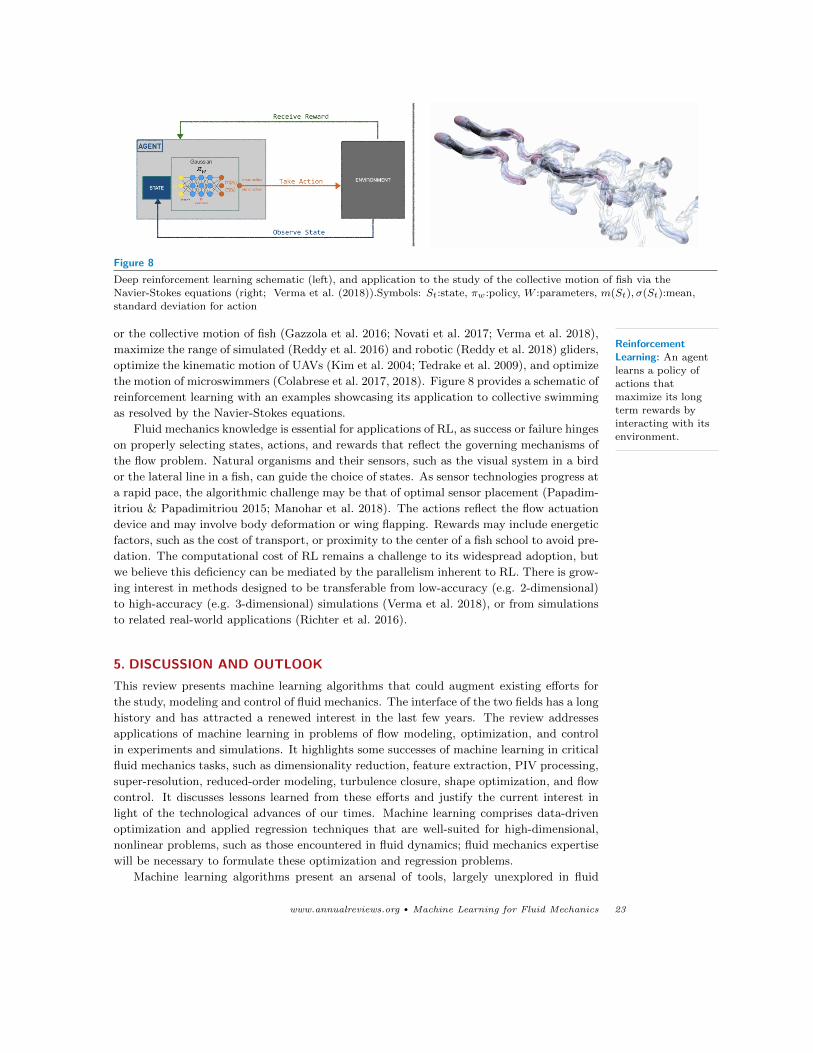
Figure 8

Deep reinforcement learning schematic (left), and application to the study of the collective motion of fish via the

Navier-Stokes equations (right; Verma et al. (2018)).Symbols: St:state, πw:policy, W :parameters, m(St), σ(St):mean,standard deviation for action

or the collective motion of fish (Gazzola et al. 2016; Novati et al. 2017; Verma et al. 2018),

maximize the range of simulated (Reddy et al. 2016) and robotic (Reddy et al. 2018) gliders,

optimize the kinematic motion of UAVs (Kim et al. 2004; Tedrake et al. 2009), and optimize

the motion of microswimmers (Colabrese et al. 2017, 2018). Figure 8 provides a schematic of

reinforcement learning with an examples showcasing its application to collective swimming

as resolved by the Navier-Stokes equations.

ReinforcementLearning: An agent

learns a policy ofactions that

maximize its long

term rewards byinteracting with its

environment.Fluid mechanics knowledge is essential for applications of RL, as success or failure hinges

on properly selecting states, actions, and rewards that reflect the governing mechanisms of

the flow problem. Natural organisms and their sensors, such as the visual system in a bird

or the lateral line in a fish, can guide the choice of states. As sensor technologies progress at

a rapid pace, the algorithmic challenge may be that of optimal sensor placement (Papadim-

itriou & Papadimitriou 2015; Manohar et al. 2018). The actions reflect the flow actuation

device and may involve body deformation or wing flapping. Rewards may include energetic

factors, such as the cost of transport, or proximity to the center of a fish school to avoid pre-

dation. The computational cost of RL remains a challenge to its widespread adoption, but

we believe this deficiency can be mediated by the parallelism inherent to RL. There is grow-

ing interest in methods designed to be transferable from low-accuracy (e.g. 2-dimensional)

to high-accuracy (e.g. 3-dimensional) simulations (Verma et al. 2018), or from simulations

to related real-world applications (Richter et al. 2016).

5. DISCUSSION AND OUTLOOK

This review presents machine learning algorithms that could augment existing efforts for

the study, modeling and control of fluid mechanics. The interface of the two fields has a long

history and has attracted a renewed interest in the last few years. The review addresses

applications of machine learning in problems of flow modeling, optimization, and control

in experiments and simulations. It highlights some successes of machine learning in critical

fluid mechanics tasks, such as dimensionality reduction, feature extraction, PIV processing,

super-resolution, reduced-order modeling, turbulence closure, shape optimization, and flow

control. It discusses lessons learned from these efforts and justify the current interest in

light of the technological advances of our times. Machine learning comprises data-driven

optimization and applied regression techniques that are well-suited for high-dimensional,

nonlinear problems, such as those encountered in fluid dynamics; fluid mechanics expertise

will be necessary to formulate these optimization and regression problems.

Machine learning algorithms present an arsenal of tools, largely unexplored in fluid


mechanics research, that can augment existing modes of inquiry. Fluid mechanics knowledge

and centuries old principles such as conservation laws remain relevant in the era of big data.

Such knowledge can help frame more precise questions and assist in reducing the large

computational cost often associated with the application of machine learning algorithms

in flow control and optimization. The exploration and visualization of high-dimensional

search spaces will be dramatically simplified by machine learning and increasingly capable

high-performance computing resources.

In the near future, experience with machine learning algorithms will help frame new

questions in fluid mechanics, extending decades old linearized models and linear approaches

to the nonlinear regime. The transition to the nonlinear realm of machine learning is facil-

itated by the abundance of open source software and methods, and the prevalent openness

of the ML community. In the long term machine learning will undoubtedly offer a fresh

look into old problems of fluid mechanics under the light of data. Interpreting the machine

learning solutions, and refining the problem statement, will again require fluid mechanics

expertise.

A word of caution is necessary to balance the current excitement about data-driven

research and the (almost magical) powers of machine learning. After all a machine learn-

ing algorithm will always provide some kind of answer to any question, that is based on

its training data; data that may not be even relevant to the question at hand. Properly

formulating the question, selecting the data as well as the learning machine and its training

is a process where all parts are critical. Applying machine learning algorithms to fluid

mecahnics is faced with numerous outstanding challenges (and opportunities!). Although

many fields of machine learning are concerned with raw predictive performance, applica-

tions in fluid mechanics often require models that are explainable, generalizable, and have

guarantees.

Although deep learning will undoubtedly become a critical tool in several aspects of flow

modeling, not all machine learning is deep learning. It is important to consider several fac-

tors when choosing methods, including the quality and quantity of data, the desired inputs

and outputs, the cost function to be optimized, whether or not the task involves interpola-

tion or extrapolation, and how important it is for models to be explainable. It is important

to cross-validate machine learned models, otherwise results may be prone to overfitting.

It is also important to develop and adapt machine learning algorithms that are not only

physics informed but also physics consistent, a major outstanding challenge in artificial in-

telligence. This review concludes with a call for action in the fluid mechanics community to

further embrace open and reproducible research products and standards. Reproducibility is

a cornerstone of science and a number of frameworks are currently developed to render this

intop a systematic scientifc process (Barber (2015)). It is increasingly possible to document

procedures, archive code, and host data so that others can reproduce results. Data is essen-

tial for machine learning; thus, creating and curating benchmark datasets and software will

spur interest among researchers in related fields, driving progress. These fluid benchmarks

are more challenging than the “traditional” image data sets encountered in machine learn-

ing: fluids data is multi-modal and multi-fidelity; it has high-resolution in some dimensions

and is sparse in others; many tasks balance multiple objectives; and foremost, our data

comes from a dynamical system, where many tasks do not admit post-mortem analysis.

We are entering a new era in fluid mechanics research. Centuries of theoretical devel-

opments based on first principles are merging with data-driven analysis. This fusion could

provide solutions to many long-sought problems in fluid dynamics and offers new hope for


enhanced understanding of turbulence and its governing mechanisms.Reproducibility: Theprocess of

documenting

procedures,archiving code and

data so that

scientific results canbe readily

reproducible.

SUMMARY POINTS

1. Machine learning entails powerful information processing algorithms that are rele-

vant for modeling, optimization, and control of fluid flows. Effective problem solvers

will have expertise in machine learning and in-depth knowledge of fluid mechanics.

2. Fluid mechanics has been traditionally concerned with big data. For decades it has

used machine learning to understand, predict, optimize, and control flows. Cur-

rently, machine learning capabilities are advancing at an unprecedented rate, and

fluid mechanics is beginning to tap into the full potential of these powerful methods.

3. Many tasks in fluid mechanics, such as reduced-order modeling, shape optimization,

and feedback control, may be posed as optimization and regression tasks. Machine

learning can dramatically improve optimization performance and reduce conver-

gence time. Machine learning is also used for dimensionality reduction, identifying

low-dimensional manifolds and discrete flow regimes, which benefit understanding.

4. Flow control strategies have been traditionally based on the precise sequence: start

with understanding, follow with modeling and then control. The machine-learning

paradigm suggests more flexibility in this sequence and iterations between data

driven and first principle approaches.

FUTURE ISSUES

1. Machine learning algorithms often come without guarantees for performance, ro-

bustness, or convergence, even for well-defined tasks. How can interpretability,

generalizability, and explainability of the results be achieved?

2. Incorporating and enforcing known flow physics is a challenge and opportunity for

machine learning algorithms. Can we hybridize effectively data driven and first

principle approaches in fluid mechanics?

3. There are many possibilities to discover new physical mechanisms, symmetries,

constraints, and invariances from fluid mechanics data.

4. Data driven modeling can be a potent alternative in revisiting existing empirical

laws in fluid mechanics.

5. Machine learning encourages open sharing of data and software. Can this assist the

development of frameworks for reproducible and open science in fluid mechanics?

6. Fluids researchers will benefit from interfacing with the machine learning commu-

nity, where the latest advances are reported in peer reviewed conferences.

DISCLOSURE STATEMENT

The authors are not aware of any affiliations, memberships, funding, or financial holdings

that might be perceived as affecting the objectivity of this review.

ACKNOWLEDGMENTS

SLB acknowledges funding from the Army Research Office (ARO W911NF-17-1-0306,

W911NF-17-1-0422) and the Air Force Office of Scientific Research (AFOSR FA9550-18-

1-0200). BRN acknowledges funding by LIMSI-CNRS, Universite Paris Sud (SMEMaG),


the French National Research Agency (ANR-11-IDEX-0003-02, ANR-17-ASTR-0022) and

the German Research Foundation (CRC880, SE 2504/2-1, SE 2504/3-1). PK acknowledges

funding from the ERC Advanced Investigator Award (FMCoBe, No. 34117), the Swiss

National Science Foundation and the Swiss Supercomputing center (CSCS). We are grate-

ful for discussions with Nathan Kutz (University of Washington), Jean-Christophe Loiseau

(ENSAM ParisTech, Paris), Francois Lusseyran (LIMSI-CNRS, Paris), Guido Novati (ETH

Zurich), Luc Pastur (ENSTA ParisTech, Paris), and Pantelis Vlachas (ETH Zurich).

LITERATURE CITED

Adrian RJ. 1991. Particle-imaging techniques for experimental fluid mechanics. Annu. Rev. Fluid

Mech. 23:261–304

Alsalman M, Colvert B, Kanso E. 2018. Training bioinspired sensors to classify flows. Bioinspiration

Biomim. 14:016009

Amsallem D, Zahr MJ, Farhat C. 2012. Nonlinear model order reduction based on local reduced-

order bases. Int. J. Numer. Meth. Engin. 92:891–916

Andrychowicz M, Wolski F, Ray A, Schneider J, Fong R, et al. 2017. Hindsight experience replay,

In Adv. Neural Inf. Process. Syst.

Bai Z, Wimalajeewa T, Berger Z, Wang G, Glauser M, Varshney PK. 2014. Low-dimensional ap-

proach for reconstruction of airfoil data via compressive sensing. AIAA J. 53:920–933How linear PCA

(or POD) connects

to linear neural

networks.

Baldi P, Hornik K. 1989. Neural networks and principal component analysis: Learning

from examples without local minima. Neural Netw. 2:53–58

Barber D. 2012. Bayesian inference and machine learning. Cambridge University Press

Reproducible

science: a

framework.

Barber, R. F. and Candes E. J., 2015. Controlling the false discovery rate via knock-

offs. Annals of Statistics 43:2055-2085

Battaglia PW, Hamrick JB, Bapst V, Sanchez-Gonzalez A, Zambaldi V, et al. 2018. Relational

inductive biases, deep learning, and graph networks. arXiv preprint arXiv:1806.01261

Bellman R. 1952. On the theory of dynamic programming. Proc. Natl. Acad. Sci. USA 38:716–719

Benard N, Pons-Prats J, Periaux J, Bugeda G, Braud P, et al. 2016. Turbulent separated shear flow

control by surface plasma actuator: experimental optimization by genetic algorithm approach.

Exp. Fluids 57:22:1–17

Bewley TR, Moin P, Temam R. 2001. DNS-based predictive control of turbulence: an optimal

benchmark for feedback algorithms. J. Fluid Mech. 447:179–225

Bishop CM, James GD. 1993. Analysis of multiphase flows using dual-energy gamma densitometry

and neural networks. Nucl. Instrum. Methods Phys. Res. 327:580–593Theoretical

Analysis of the

approximation

properties of deep

neural networks.

Bolcskei H, Grohs P, Kutyniok G, Petersen P. 2019. Optimal approximation with

sparsely connected deep neural networks. SIAM J. Math. Data Sci. 1:8–45

Bourguignon JL, Tropp JA, Sharma AS, McKeon BJ. 2014. Compact representation of wall-bounded

turbulence using compressive sampling. Phys. Fluids 26:015109

Bousmalis K, Irpan A, Wohlhart P, Bai Y, Kelcey M, et al. 2017. Using simulation and domain

adaptation to improve efficiency of deep robotic grasping. arXiv preprint arXiv:1709.07857

Breiman L. 2001. Random forests. Mach. Learn. 45:5–32

Bright I, Lin G, Kutz JN. 2013. Compressive sensing and machine learning strategies for character-

izing the flow around a cylinder with limited pressure measurements. Phys. Fluids 25:1–15

Brunton SL, Kutz JN. 2019. Data-driven science and engineering: Machine learning, dynamical

systems, and control. Cambridge University Press

Brunton SL, Noack BR. 2015. Closed-loop turbulence control: Progress and challenges. Appl. Mech.

Rev. 67:1–48

Brunton SL, Proctor JL, Kutz JN. 2016. Discovering governing equations from data by sparse

identification of nonlinear dynamical systems. Proc. Natl. Acad. Sci. USA 113:3932–3937

Bueche D, Stoll P, Dornberger R, Koumoutsakos P. 2002. Multi-objective evolutionary algorithm for

the optimization of noisy combustion problems. IEEE Trans. Syst. Man. Cybern. C 32:460–473


http://arxiv.org/abs/1806.01261


Chen TQ, Rubanova Y, Bettencourt J, Duvenaud DK. 2018. Neural ordinary differential equa-

tions. In Advances in Neural Information Processing Systems 31, eds. S Bengio, H Wallach,

H Larochelle, K Grauman, N Cesa-Bianchi, R Garnett. Curran Associates, Inc., 6571–6583

Cherkassky V, Mulier FM. 2007. Learning from data: concepts, theory, and methods. John Wiley

& Sons

Colabrese S, Gustavsson K, Celani A, Biferale L. 2017. Flow navigation by smart microswimmers

via reinforcement learning. Phys. Rev. Lett. 118:158004

Colabrese S, Gustavsson K, Celani A, Biferale L. 2018. Smart inertial particles. Phys. Rev. Fluids

3:084301

Colvert B, Alsalman M, Kanso E. 2018. Classifying vortex wakes using neural networks. Bioinspi-

ration Biomim. 13:025003

Dissanayake M, Phan-Thien N. 1994. Neural-network-based approximations for solving partial dif-

ferential equations. Comm. Numer. Meth. Eng. 10:195–201

Dong C, Loy CC, He K, Tang X. 2014. Learning a deep convolutional network for image super-

resolution, In Comput. Vis. ECCV. Springer

Donoho, D.L., 2006. Compressed Sensing, In IEEE Transactions on Information Theory. 52:1289-

1306

Dracopoulos DC. 1997. Evolutionary learning algorithms for neural adaptive control. Perspectives

in Neural Computing. London, etc.: Springer-Verlag

Duraisamy K, Iaccarino G, Xiao H. 2019. Turbulence modeling in the age of data. Annu. Rev. Fluid

Mech. 51:357–377

Duriez T, Brunton SL, Noack BR. 2016. Machine learning control: Taming nonlinear dynamics and

turbulence. Springer

Faller WE, Schreck SJ. 1996. Neural networks: applications and opportunities in aeronautics. Prog.

Aerosp. Sci. 32:433–456

Fleming PJ, Purshouse RC. 2002. Evolutionary algorithms in control systems engineering: a survey.

Control Eng. Pract. 10:1223–1241

Freeman WT, Jones TR, Pasztor EC. 2002. Example-based super-resolution. IEEE Comput. Graph.

22:56–65

Fukami K, Fukagata K, Taira K. 2018. Super-resolution reconstruction of turbulent flows with

machine learning. arXiv preprint arXiv:1811.11328

Gardner E. 1988. The space of interactions in neural network models. J. Phys. A 21:257

Gazzola M, Hejazialhosseini B, Koumoutsakos P. 2014. Reinforcement learning and wavelet adapted

vortex methods for simulations of self-propelled swimmers. SIAM J. Sci. Comp. 36:B622–B639

Gazzola M, Tchieu A, Alexeev D, De Brauer A, Koumoutsakos P. 2016. Learning to school in the

presence of hydrodynamic interactions. J. Fluid Mech. 789

Gazzola M, Van Rees WM, Koumoutsakos P. 2012. C-start: optimal start of larval fish. J. Fluid

Mech. 698:5–18

Germano M, Piomelli U, Moin P, Cabot WH. 1991. A dynamic subgrid-scale eddy viscosity model.

Phys. Fluids 3:1760–1765

Giannakoglou K, Papadimitriou D, Kampolis I. 2006. Aerodynamic shape design using evolutionary

algorithms and new gradient-assisted metamodels. Comput. Methods Appl. Mech. Eng. 195:6312–

6329

Glaz B, Liu L, Friedmann PP. 2010. Reduced-order nonlinear unsteady aerodynamic modeling using

a surrogate-based recurrence framework. AIAA J. 48:2418–2429

Gonzalez-Garcia R, Rico-Martinez R, Kevrekidis I. 1998. Identification of distributed parameter

systems: A neural net based approach. Comput. Chem. Eng. 22:S965–S968

Goodfellow I, Bengio Y, Courville A. 2016. Deep learning. MIT PressPowerful deep

learning

architecture that

learns through a

game between a

network that can

“generate” new

data and a network

that is an expert

classifier.

Goodfellow I, Pouget-Abadie J, Mirza M, Xu B, Warde-Farley D, et al. 2014. Gener-

ative adversarial nets, In Adv. Neural Inf. Process. Syst.

Grant I, Pan X. 1995. An investigation of the performance of multi layer, neural networks applied



to the analysis of PIV images. Exp. Fluids 19:159–166

Graves A, Fernandez S, Schmidhuber J. 2007. Multi-dimensional recurrent neural networks. Artifi-

cial Neural Networks–ICANN :549—-558

Gueniat F, Mathelin L, Hussaini MY. 2016. A statistical learning strategy for closed-loop control

of fluid flows. Theor. Comp. Fluid Dyn. 30:497–510

Halko N, Martinsson PG, Tropp JA. 2011. Finding structure with randomness: Probabilistic algo-

rithms for constructing approximate matrix decompositions. SIAM Rev. 53:217–288

Hamdaoui M, Chaskalovic J, Doncieux S, Sagaut P. 2010. Using multiobjective evolutionary algo-

rithms and data-mining methods to optimize ornithopters’ kinematics. J. Aircraft 47:1504

Hansen N, Muller SD, Koumoutsakos P. 2003. Reducing the time complexity of the derandomized

evolution strategy with covariance matrix adaptation (CMA-ES). Evol. Comput. 11:1–18

Hansen N, Niederberger AS, Guzzella L, Koumoutsakos P. 2009. A method for handling uncertainty

in evolutionary optimization with an application to feedback control of combustion. IEEE Trans.

Evol. Comput. 13:180–197

Hastie T, Tibshirani R, Friedman J, Hastie T, Friedman J, Tibshirani R. 2009. The elements of

statistical learning, vol. 2. Springer

Hinton GE, Sejnowski TJ. 1986. Learning and releaming in Boltzmann machines, In Parallel Dis-

tributed Processing: Explorations in the Microstructure of Cognition, vol. 1. MIT PressRegularization of

recurrent neural

networks, and

major contributor

to the success of

Google translate.

Hochreiter S, Schmidhuber J. 1997. Long short-term memory. Neural Comput. 9:1735–

1780

Holland JH. 1975. Adaptation in natural and artificial systems: An introductory analysis with

applications to biology, control, and artificial intelligence. University of Michigan Press

Hopfield JJ. 1982. Neural networks and physical systems with emergent collective computational

abilities. Proc. Natl. Acad. Sci. USA 79:2554–2558

Hornik K, Stinchcombe M, White H. 1989. Multilayer feedforward networks are universal approxi-

mators. Neural Netw. 2:359–366

Hou W, Darakananda D, Eldredge J. 2019. Machine learning based detection of flow disturbances

using surface pressure measurements, In AIAA Scitech

Jambunathan K, Hartle S, Ashforth-Frost S, Fontama V. 1996. Evaluating convective heat transfer

coefficients using neural networks. Int. J. Heat Mass Transf. 39:2329–2332

Kaiser E, Noack BR, Cordier L, Spohn A, Segond M, et al. 2014. Cluster-based reduced-order

modelling of a mixing layer. J. Fluid Mech. 754:365–414

Kern S, Muller SD, Hansen N, Buche D, Ocenasek J, Koumoutsakos P. 2004. Learning Probability

Distributions in Continuous Evolutionary Algorithms – A Comparative Review. Nat. Comput.

3:77–112

Kim B, Azevedo VC, Thuerey N, Kim T, Gross M, Solenthaler B. 2018. Deep fluids: A generative

network for parameterized fluid simulations. arXiv preprint arXiv:1806.02071

Kim HJ, Jordan MI, Sastry S, Ng AY. 2004. Autonomous helicopter flight via reinforcement learning,

In Adv. Neural Inf. Process. Syst.

Knaak M, Rothlubbers C, Orglmeister R. 1997. A Hopfield neural network for flow field computation

based on particle image velocimetry/particle tracking velocimetry image sequences. IEEE Int.

Conf. Neural Netw. 1:48–52

Kohonen T. 1995. Self-organizing maps. Springer Verlag

Kolmogorov A. 1941. The local structure of turbulence in incompressible viscous fluid for very large

Reynolds number. Dokl. Akad. Nauk SSSR 30:9–13. (translated and reprinted 1991 in Proc. R.

Soc. Lond. A 434, 9–13)

Koza JR. 1992. Genetic Programming: On the Programming of Computers by Means of Natural

Selection. Boston: The MIT Press

Krizhevsky A, Sutskever I, Hinton GE. 2012. Imagenet classification with deep convolutional neural

networks, In Adv. Neural Inf. Process. Syst.

Kutz JN, Brunton SL, Brunton BW, Proctor JL. 2016. Dynamic mode decomposition: Data-driven



modeling of complex systems. SIAM

Labonte G. 1999. A new neural network for particle-tracking velocimetry. Exp. Fluids 26:340–346

Lagaris IE, Likas A, Fotiadis DI. 1998. Artificial neural networks for solving ordinary and partial

differential equations. IEEE Trans. Neural Netw. 9:987–1000

LeCun Y, Bengio Y, Hinton G. 2015. Deep learning. Nature 521:436–444

Lee C, Kim J, Babcock D, Goodman R. 1997. Application of neural networks to turbulence control

for drag reduction. Phys. Fluids 9:1740–1747

Lee Y, Yang H, Yin Z. 2017. PIV-DCNN: cascaded deep convolutional neural networks for particle

image velocimetry. Exp. Fluids 58:171

Li Q, Dietrich F, Bollt EM, Kevrekidis IG. 2017. Extended dynamic mode decomposition with

dictionary learning: A data-driven adaptive spectral decomposition of the Koopman operator.

Chaos 27:103111

Liang D, Jiang C, Li Y. 2003. Cellular neural network to detect spurious vectors in PIV data. Exp.

Fluids 34:52–62

Ling J, Jones R, Templeton J. 2016a. Machine learning strategies for systems with invariance

properties. J. Comp. Phys. 318:22–35

Ling J, Kurzawski A, Templeton J. 2016b. Reynolds averaged turbulence modelling using deep

neural networks with embedded invariance. J. Fluid Mech. 807:155–166

Ling J, Templeton J. 2015. Evaluation of machine learning algorithms for prediction of regions of

high Reynolds averaged Navier Stokes uncertainty. Phys. Fluids 27:085103

Loiseau JC, Brunton SL. 2018. Constrained sparse Galerkin regression. J. Fluid Mech. 838:42–67

Loucks D, van Beek E, Stedinger J, Dijkman J, Villars M. 2005. Water resources systems planning

and management: An introduction to methods, vol. 2. Springer International Publishing

Lumley J. 1970. Stochastic tools in turbulence. New York: Academic Press

Lusch B, Kutz JN, Brunton SL. 2018. Deep learning for universal linear embeddings of nonlinear

dynamics. Nat. Commun. 9:4950

Mahoney MW. 2011. Randomized algorithms for matrices and data. Foundations and Trends in

Machine Learning 3:123–224

Manohar K, Brunton BW, Kutz JN, Brunton SL. 2018. Data-driven sparse sensor placement. IEEE

Control Syst. Mag. 38:63–86

Mardt A, Pasquali L, Wu H, Noe F. 2018. VAMPnets: Deep learning of molecular kinetics. Nat.

Commun. 9

Martin N, Gharib M. 2018. Experimental trajectory optimization of a flapping fin propulsor using

an evolutionary strategy. Bioinspiration Biomim. 14:016010

Maulik R, San O, Rasheed A, Vedula P. 2019. Subgrid modelling for two-dimensional turbulence

using neural networks. J. Fluid Mech. 858:122–144

Meena MG, Nair AG, Taira K. 2018. Network community-based model reduction for vortical flows.

Phys. Rev. E 97:063103

Mehta UB, Kutler P. 1984. Computational aerodynamics and artificial intelligence. Technical Mem-

orandum 85994, NASA

Meijering E. 2002. A chronology of interpolation: from ancient astronomy to modern signal and

image processing. Proc. IEEE 90:319–342

Meneveau C, Katz J. 2000. Scale-invariance and turbulence models for large-eddy simulation. Annu.

Rev. Fluid Mech. 32:1–32

Mezic I. 2013. Analysis of fluid flows via spectral properties of the Koopman operator. Annu. Rev.

Fluid Mech. 45:357–378

Milano M, Koumoutsakos P. 2002. Neural network modeling for near wall turbulent flow. J. Comp.

Phys. 182:1–26

Minsky M, Papert SA. 1969. Perceptrons: An introduction to computational geometry. MIT Press

Mnih V, Kavukcuoglu K, Silver D, Rusu Aa, Veness J, et al. 2015. Human-level control through

deep reinforcement learning. Nature 518:529–533


Nair AG, Taira K. 2015. Network-theoretic approach to sparsified discrete vortex dynamics. J. Fluid

Mech. 768:549–571

Noack BR. 2018. Closed-loop turbulence control—From human to machine learning (and retour),

In Proc. FSSIC, eds. Y Zhou, M Kimura, G Peng, AD Lucey, L Hung. Springer

Noe F, Nuske F. 2013. A variational approach to modeling slow processes in stochastic dynamical

systems. SIAM Multiscale Model Simul. 11:635–655

Novati G, Mahadevan L, Koumoutsakos P. 2019. Controlled gliding and perching through deep

reinforcement learning. Physical Review Fluids

Novati G, Verma S, Alexeev D, Rossinelli D, Van Rees WM, Koumoutsakos P. 2017. Synchronisation

through learning for two self-propelled swimmers. Bioinspiration Biomim. 12:aa6311

Nuske F, Schneider R, Vitalini F, Noe F. 2016. Variational tensor approach for approximating the

rare-event kinetics of macromolecular systems. J. Chem. Phys. 144:054105

Ollivier Y, Arnold L, Auger A, Hansen N. 2017. Information-geometric optimization algorithms: A

unifying picture via invariance principles. J. Mach. Learn. Res. 18:564–628

Ostermeier A, Gawelczyk A, Hansen N. 1994. Step-size adaptation based on non-local use of selection

information. Internat. Conf. PPSN

Ouellette NT, Xu H, Bodenschatz E. 2006. A quantitative study of three-dimensional Lagrangian

particle tracking algorithms. Exp. Fluids 40:301–313

Papadimitriou DI, Papadimitriou C. 2015. Optimal Sensor Placement for the Estimation of Turbu-

lent Model Parameters in CFD. Int. J. Uncert. Quant. 5:545–568

Parish EJ, Duraisamy K. 2016. A paradigm for data-driven predictive modeling using field inversion

and machine learning. J. Comp. Phys. 305:758–774

Pathak J, Hunt B, Girvan M, Lu Z, Ott E. 2018. Model-free prediction of large spatiotemporally

chaotic systems from data: a reservoir computing approach. Phys. Rev. Lett. 120:024102

Pelikan M, Ocenasek J, Trebst S, Troyer M, Alet F. 2004. Computational complexity and simulation

of rare events of ising spin glasses. Genetic and Evolutionary Computation–GECCO :36–47

Perdikaris P, Venturi D, Karniadakis G. 2016. Multifidelity information fusion algorithms for high-

dimensional systems and massive data sets. SIAM J. Sci. Comput. 38:B521–B538

Perlman E, Burns R, Li Y, Meneveau C. 2007. Data exploration of turbulence simulations using a

database cluster, In ACM/IEEE Conf. Supercomp.

Phan MQ, Juang JN, Hyland DC. 1995. On neural networks in identification and control of dynamic

systems, In Wave Motion, Intelligent Structures And Nonlinear Mechanics

Pierret S, Van den Braembussche R. 1998. Turbomachinery blade design using a Navier-Stokes

solver and artificial neural network. ASME Intern. Gas Turb. Aeroeng. Cong. Exh.

Pollard A, Castillo L, Danaila L, Glauser M. 2016. Whither turbulence and big data in the 21st

century? Springer

Rabault J, Kuchta M, Jensen A, Reglade U, Cerardi N. 2019. Artificial neural networks trained

through deep reinforcement learning discover control strategies for active flow control. J. Fluid

Mech. 865:281–302

Raissi M, Karniadakis GE. 2018. Hidden physics models: Machine learning of nonlinear partial

differential equations. J. Comp. Phys. 357:125–141

Raissi M, Perdikaris P, Karniadakis G. 2019. Physics-informed neural networks: A deep learn-

ing framework for solving forward and inverse problems involving nonlinear partial differential

equations. J. Comp. Phys. 378:686–707

Rechenberg I. 1964. Kybernetische losungsansteuerung einer experimentellen forschungsaufgabe, In

Ann. Conf. WGLR Berlin, vol. 35

Rechenberg I. 1973. Evolutionsstrategie: Optimierung technischer Systeme nach Prinzipien der

biologischen Evolution. Stuttgart: Frommann-Holzboog

Reddy G, Celani A, Sejnowski TJ, Vergassola M. 2016. Learning to soar in turbulent environments.

Proc. Natl. Acad. Sci. USA 113:E4877–E4884

Reddy G, Wong-Ng J, Celani A, Sejnowski TJ, Vergassola M. 2018. Glider soaring via reinforcement


learning in the field. Nature 562:236–239

Richter SR, Vineet V, Roth S, Koltun V. 2016. Playing for data: Ground truth from computer

games, In Comput. Vis. ECCV. Springer

Rico-Martinez R., Krischer K., Kevrekidis I.G., Kube M.C., Hudson J.L., 1992. Discrete-vs.

continuous-time nonlinear signal processing of Cu electrodissolution data Chem. Eng. Commun

118:25-48

Rokhlin V, Szlam A, Tygert M. 2009. A randomized algorithm for principal component analysis.

SIAM J. Matrix Anal. Appl. 31:1100–1124First example of a

simple binary

network with

learning

capabilities

Rosenblatt F. 1958. The perceptron: a probabilistic model for information storage and

organization in the brain. Psychol. Rev. 65:386

Rowley CW, Dawson S. 2016. Model reduction for flow analysis and control. Annu. Rev. Fluid

Mech. 49

Rowley CW, Mezic I, Bagheri S, Schlatter P, Henningson D. 2009. Spectral analysis of nonlinear

flows. J. Fluid Mech. 645:115–127

Rudy SH, Brunton SL, Proctor JL, Kutz JN. 2017. Data-driven discovery of partial differential

equations. Sci. Adv. 3

Rumelhart DE, Hinton GE, Williams RJ, et al. 1986. Learning representations by back-propagating

errors. Nature 323:533–536

Salimans T, Ho J, Chen X, Sutskever I. 2017. Evolution strategies as a scalable alternative to

reinforcement learning. arXiv preprint arXiv:1703.03864

Schaeffer H. 2017. Learning partial differential equations via data discovery and sparse optimization,

In Proc. R. Soc. A, vol. 473. The Royal Society

Schaul T, Horgan D, Gregor K, Silver D. 2015. Universal value function approximators, In ICML

Schmid PJ. 2010. Dynamic mode decomposition for numerical and experimental data. J. Fluid

Mech. 656:5–28

Schmidt M, Lipson H. 2009. Distilling free-form natural laws from experimental data. Science

324:81–85

Scholkopf B, Smola AJ. 2002. Learning with kernels: support vector machines, regularization,

optimization, and beyond. MIT Press

Schwefel HP. 1977. Numerische optimierung von computer-modellen mittels der evolutionsstrate-

gie.(teil 1, kap. 1-5). Birkhauser

Semeraro O, Lusseyran F, Pastur L, Jordan P. 2016. Qualitative dynamics of wavepackets in tur-

bulent jets. arXiv preprint arXiv:1608.06750

Silver D, Huang A, Maddison CJ, Guez A, Sifre L, et al. 2016. Mastering the game of Go with deep

neural networks and tree search. Nature 529:484–489

Singh AP, Medida S, Duraisamy K. 2017. Machine-learning-augmented predictive modeling of tur-

bulent separated flows over airfoils. AIAA J. 55:2215–2227

Sirovich L. 1987. Turbulence and the dynamics of coherent structures, parts I-III. Q. Appl. Math.

XLV:561–590

Sirovich L, Kirby M. 1987. A low-dimensional procedure for the characterization of human faces.

J. Opt. Soc. Am. A 4:519–524

Skinner SN, Zare-Behtash H. 2018. State-of-the-art in aerodynamic shape optimisation methods.

Appl. Soft. Comput. 62:933–962

Strom B, Brunton SL, Polagye B. 2017. Intracycle angular velocity control of cross-flow turbines.

Nat. Energy 2:1–9The classic book

for reinforcement

learning

Sutton RS, Barto AG. 2018. Reinforcement learning: An introduction, vol. 2nd Edi-

tion. MIT Press

Taira K, Brunton SL, Dawson S, Rowley CW, Colonius T, et al. 2017. Modal analysis of fluid flows:

An overview. AIAA J. 55:4013–4041

Takeishi N, Kawahara Y, Yairi T. 2017. Learning koopman invariant subspaces for dynamic mode

decomposition, In Adv. Neural Inf. Process. Syst.




Tedrake R, Jackowski Z, Cory R, Roberts JW, Hoburg W. 2009. Learning to fly like a bird, In 14th

ISRR

Teo C, Lim K, Hong G, Yeo M. 1991. A neural net approach in analysing photographs in PIV.

IEEE Sys. Man. Cybern. 3:1535–1538

Tesauro G. 1992. Practical Issues in Temporal Difference Learning. Mach. Learn. 8:257–277An excellent

resource linking

machine learning

and Bayesian

inference

algorithms.

Theodoridis S. 2015. Machine learning: a Bayesian and optimization perspective. Aca-

demic Press

Tsiotras P, Mesbahi M. 2017. Toward an algorithmic control theory. J. Guid. Ctrl. Dyn. 40:194–196

Van Rees WM, Gazzola M, Koumoutsakos P. 2015. Optimal morphokinematics for undulatory

swimmers at intermediate reynolds numbers. J. Fluid Mech. 775:178–188

Verma S, Novati G, Koumoutsakos P. 2018. Efficient collective swimming by harnessing vortices

through deep reinforcement learning. Proc. Natl. Acad. Sci. USA 115

Vlachas PR, Byeon W, Wan ZY, Sapsis TP, Koumoutsakos P. 2018. Data-driven forecasting

of high-dimensional chaotic systems with long short-term memory networks. Proc. R. Soc. A

474:20170844

Wan ZY, Vlachas P, Koumoutsakos P, Sapsis T. 2018. Data-assisted reduced-order modeling of

extreme events in complex dynamical systems. PLoS ONE 13:e0197704

Wang JX, Wu JL, Xiao H. 2017. Physics-informed machine learning approach for reconstructing

Reynolds stress modeling discrepancies based on DNS data. Phys. Rev. Fluids 2:034603

Wang M, Hemati MS. 2017. Detecting exotic wakes with hydrodynamic sensors. arXiv preprint

arXiv:1711.10576

Wehmeyer C, Noe F. 2018. Time-lagged autoencoders: Deep learning of slow collective variables

for molecular kinetics. J. Chem. Phys. 148:1–9

Wiener N. 1965. Cybernetics or control and communication in the animal and the machine, vol. 25.

MIT Press

Willert CE, Gharib M. 1991. Digital particle image velocimetry. Exp. Fluids 10:181–193

Williams MO, Rowley CW, Kevrekidis IG. 2015. A kernel approach to data-driven Koopman spec-

tral analysis. J. Comp. Dyn. 2:247–265

Wright J, Yang A, Ganesh A, Sastry S, Ma Y. 2009. Robust face recognition via sparse representa-

tion. IEEE Trans. Pattern Anal. Mach. Intell. 31:210–227

Wu H, Mardt A, Pasquali L, Noe F. 2018. Deep generative markov state models. Adv. Neural Inf.

Process. Syst.

Wu X, Moin P. 2008. A direct numerical simulation study on the mean velocity characteristics in

turbulent pipe flow. J. Fluid Mech. 608:81–112

Xiao H, Wu JL, Wang JX, Sun R, Roy C. 2016. Quantifying and reducing model-form uncertain-

ties in Reynolds-averaged Navier–Stokes simulations: A data-driven, physics-informed Bayesian

approach. J. Comp. Phys. 324:115–136

Xie Y, Franz E, Chu M, Thuerey N. 2018. tempoGAN: A temporally coherent, volumetric GAN for

super-resolution fluid flow. ACM Trans. Graph. 37:95

Yang J, Wright J, Huang TS, Ma Y. 2010. Image super-resolution via sparse representation. IEEE

Trans. Image Process. 19:2861–2873



Machine Learning for Fluid Mechanics - arxiv.org

Documents

Transcript of Machine Learning for Fluid Mechanics - arxiv.org