Machine Learning Department School of Computer Science ...mgormley/courses/10601/slides/... ·...
30
HMMs + Bayesian Networks 1 10-601 Introduction to Machine Learning Matt Gormley Lecture 21 Apr. 01, 2020 Machine Learning Department School of Computer Science Carnegie Mellon University
Transcript of Machine Learning Department School of Computer Science ...mgormley/courses/10601/slides/... ·...

HMMs+
Bayesian Networks
1
10-601 Introduction to Machine Learning
Matt GormleyLecture 21
Apr. 01, 2020
Machine Learning DepartmentSchool of Computer ScienceCarnegie Mellon University
Reminders
• Practice Problems for Exam 2
– Out: Fri, Mar 20
• Midterm Exam 2
– Thu, Apr 2 – evening exam, details announced onPiazza
• Homework 7: HMMs
– Out: Thu, Apr 02
– Due: Fri, Apr 10 at 11:59pm
• Today’s In-Class Poll
– http://poll.mlcourse.org
2

THE FORWARD-BACKWARD ALGORITHM
6

Forward-Backward Algorithm
7
O(K) O(K2T)
Brute force algorithm would be
O(KT)

Inference for HMMs
Whiteboard– Forward-backward algorithm
(edge weights version)– Viterbi algorithm
(edge weights version)
8

Forward-Backward Algorithm
9
O(K) O(K2T)
Brute force algorithm would be
O(KT)

Derivation of Forward Algorithm
10
Derivation:
Definition:

Viterbi Algorithm
11

Inference in HMMsWhat is the computational complexity of inference for HMMs?
• The naïve (brute force) computations for Evaluation, Decoding, and Marginals take exponential time, O(KT)
• The forward-backward algorithm and Viterbialgorithm run in polynomial time, O(T*K2)– Thanks to dynamic programming!
12

Shortcomings of Hidden Markov Models
• HMM models capture dependences between each state and only its corresponding observation – NLP example: In a sentence segmentation task, each segmental state may depend
not just on a single word (and the adjacent segmental stages), but also on the (non-local) features of the whole line such as line length, indentation, amount of white space, etc.
• Mismatch between learning objective function and prediction objective function– HMM learns a joint distribution of states and observations P(Y, X), but in a prediction
task, we need the conditional probability P(Y|X)
© Eric Xing @ CMU, 2005-2015 13
Y1 Y2 … … … Yn
X1 X2 … … … Xn
START

MBR DECODING
14

Inference for HMMs
– Three Inference Problems for an HMM1. Evaluation: Compute the probability of a given
sequence of observations
2. Viterbi Decoding: Find the most-likely sequence of hidden states, given a sequence of observations
3. Marginals: Compute the marginal distribution for a hidden state, given a sequence of observations
4. MBR Decoding: Find the lowest loss sequence of hidden states, given a sequence of observations (Viterbi decoding is a special case)
15
Four
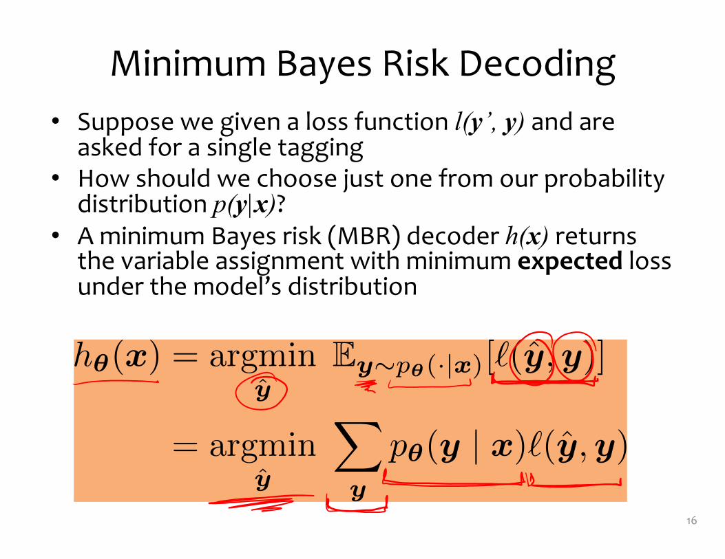
Minimum Bayes Risk Decoding• Suppose we given a loss function l(y’, y) and are
asked for a single tagging• How should we choose just one from our probability
distribution p(y|x)?• A minimum Bayes risk (MBR) decoder h(x) returns
the variable assignment with minimum expected loss under the model’s distribution
16
h✓(x) = argminy
Ey⇠p✓(·|x)[`(y,y)]
= argminy
X
y
p✓(y | x)`(y,y)

The 0-1 loss function returns 1 only if the two assignments are identical and 0 otherwise:
The MBR decoder is:
which is exactly the Viterbi decoding problem!
Minimum Bayes Risk Decoding
Consider some example loss functions:
17
`(y,y) = 1� I(y,y)
h✓(x) = argminy
X
y
p✓(y | x)(1� I(y,y))
= argmaxy
p✓(y | x)
h✓(x) = argminy
Ey⇠p✓(·|x)[`(y,y)]
= argminy
X
y
p✓(y | x)`(y,y)

The Hamming loss corresponds to accuracy and returns the number of incorrect variable assignments:
The MBR decoder is:
This decomposes across variables and requires the variable marginals.
Minimum Bayes Risk Decoding
Consider some example loss functions:
18
`(y,y) =VX
i=1
(1� I(yi, yi))
yi = h✓(x)i = argmaxyi
p✓(yi | x)
h✓(x) = argminy
Ey⇠p✓(·|x)[`(y,y)]
= argminy
X
y
p✓(y | x)`(y,y)

Learning ObjectivesHidden Markov Models
You should be able to…1. Show that structured prediction problems yield high-computation inference
problems2. Define the first order Markov assumption3. Draw a Finite State Machine depicting a first order Markov assumption4. Derive the MLE parameters of an HMM5. Define the three key problems for an HMM: evaluation, decoding, and
marginal computation
6. Derive a dynamic programming algorithm for computing the marginal probabilities of an HMM
7. Interpret the forward-backward algorithm as a message passing algorithm8. Implement supervised learning for an HMM9. Implement the forward-backward algorithm for an HMM10. Implement the Viterbi algorithm for an HMM
11. Implement a minimum Bayes risk decoder with Hamming loss for an HMM
19

Bayes Nets Outline
• Motivation– Structured Prediction
• Background– Conditional Independence– Chain Rule of Probability
• Directed Graphical Models– Writing Joint Distributions
– Definition: Bayesian Network
– Qualitative Specification– Quantitative Specification
– Familiar Models as Bayes Nets
• Conditional Independence in Bayes Nets– Three case studies
– D-separation– Markov blanket
• Learning– Fully Observed Bayes Net
– (Partially Observed Bayes Net)
• Inference– Background: Marginal Probability
– Sampling directly from the joint distribution– Gibbs Sampling
20

DIRECTED GRAPHICAL MODELSBayesian Networks
21

Example: Ryan Reynolds’ Voicemail
22From https://www.adweek.com/brand-marketing/ryan-reynolds-left-voicemails-for-all-mint-mobile-subscribers/

Example: Ryan Reynolds Voicemail
23Images from imdb.com

Example: Ryan Reynolds’ Voicemail
24From https://www.adweek.com/brand-marketing/ryan-reynolds-left-voicemails-for-all-mint-mobile-subscribers/

Directed Graphical Models (Bayes Nets)
Whiteboard– Example: Ryan Reynolds’ Voicemail
– Writing Joint Distributions• Idea #1: Giant Table
• Idea #2: Rewrite using chain rule
• Idea #3: Assume full independence
• Idea #4: Drop variables from RHS of conditionals
– Definition: Bayesian Network
25

Bayesian Network
26
p(X1, X2, X3, X4, X5) =
p(X5|X3)p(X4|X2, X3)
p(X3)p(X2|X1)p(X1)
X1
X3X2
X4 X5

Bayesian Network
• A Bayesian Network is a directed graphical model• It consists of a graph G and the conditional probabilities P• These two parts full specify the distribution:
– Qualitative Specification: G– Quantitative Specification: P
27
X1
X3X2
X4 X5
Definition:
P(X1…Xn ) = P(Xi | parents(Xi ))i=1
n
∏

Qualitative Specification
• Where does the qualitative specification come from?
– Prior knowledge of causal relationships
– Prior knowledge of modular relationships
– Assessment from experts
– Learning from data (i.e. structure learning)
– We simply prefer a certain architecture (e.g. a layered graph)
– …
© Eric Xing @ CMU, 2006-2011 28

a0 0.75a1 0.25
b0 0.33b1 0.67
a0b0 a0b1 a1b0 a1b1
c0 0.45 1 0.9 0.7c1 0.55 0 0.1 0.3
A B
C
P(a,b,c.d) =
P(a)P(b)P(c|a,b)P(d|c)
D
c0 c1
d0 0.3 0.5d1 07 0.5
Quantitative Specification
29© Eric Xing @ CMU, 2006-2011
Example: Conditional probability tables (CPTs)for discrete random variables

A B
C
P(a,b,c.d) = P(a)P(b)P(c|a,b)P(d|c)
D
A~N(μa, Σa) B~N(μb, Σb)
C~N(A+B, Σc)
D~N(μd+C, Σd)D
C
P(D|
C)
Quantitative Specification
30© Eric Xing @ CMU, 2006-2011
Example: Conditional probability density functions (CPDs)for continuous random variables

A B
C
P(a,b,c.d) = P(a)P(b)P(c|a,b)P(d|c)
D
C~N(A+B, Σc)
D~N(μd+C, Σd)
Quantitative Specification
31© Eric Xing @ CMU, 2006-2011
Example: Combination of CPTs and CPDs for a mix of discrete and continuous variables
a0 0.75a1 0.25
b0 0.33b1 0.67

Example:
Observed Variables
• In a graphical model, shaded nodes are “observed”, i.e. their values are given
32
X1
X3X2
X4 X5

Familiar Models as Bayesian Networks
33
Question:Match the model name to the corresponding Bayesian Network1. Logistic Regression2. Linear Regression3. Bernoulli Naïve Bayes4. Gaussian Naïve Bayes5. 1D Gaussian
Answer:Y
XMX1 X2 …
Y
XMX1 X2 …
Y
XMX1 X2 …
Y
XMX1 X2 …
X
µ σ2
X
A B
C D
E F

![Machine Learning Department School of Computer … › ~mgormley › courses › 10601-s19 › slides › ...(c) [2 pts.] Given the same training data, in which the points are linearly](https://static.fdocuments.net/doc/165x107/5f1cf2ede4f9a36b2d79a4fa/machine-learning-department-school-of-computer-a-mgormley-a-courses-a-10601-s19.jpg)