Special Issue: Spectroscopy and Disease

Machine Learning-Assisted Sampling ofSERS Substrates Improves Data CollectionEfficiency

Tatu Rojalin1,*, Dexter Antonio2,* , Ambarish Kulkarni2, andRandy P. Carney1

Abstract

Surface-enhanced Raman scattering (SERS) is a powerful technique for sensitive label-free analysis of chemical and bio-

logical samples. While much recent work has established sophisticated automation routines using machine learning and

related artificial intelligence methods, these efforts have largely focused on downstream processing (e.g., classification

tasks) of previously collected data. While fully automated analysis pipelines are desirable, current progress is limited by

cumbersome and manually intensive sample preparation and data collection steps. Specifically, a typical lab-scale SERS

experiment requires the user to evaluate the quality and reliability of the measurement (i.e., the spectra) as the data are

being collected. This need for expert user-intuition is a major bottleneck that limits applicability of SERS-based diagnostics

for point-of-care clinical applications, where trained spectroscopists are likely unavailable. While application-agnostic

numerical approaches (e.g., signal-to-noise thresholding) are useful, there is an urgent need to develop algorithms that

leverage expert user intuition and domain knowledge to simplify and accelerate data collection steps. To address this

challenge, in this work, we introduce a machine learning-assisted method at the acquisition stage. We tested six common

algorithms to measure best performance in the context of spectral quality judgment. For adoption into future automation

platforms, we developed an open-source python package tailored for rapid expert user annotation to train machine

learning algorithms. We expect that this new approach to use machine learning to assist in data acquisition can serve

as a useful building block for point-of-care SERS diagnostic platforms.

Keywords

Diagnostics, automation, plasmonics, surface-enhanced Raman scattering, SERS, artificial intelligence, XGBoost

Date received: 3 April 2021; accepted: 28 June 2021

Introduction

Surface-enhanced Raman scattering (SERS) is a powerful

label-free detection and analysis technique that exploits

the near-field enhancement of inelastically scattered

Raman signal via nanostructured plasmonic surfaces.1

SERS is highly sensitive, capable of even single molecule

detection, with broad applicability in detection and moni-

toring of disease, particularly for cancer. While many

proof-of-concept SERS studies emerge annually, and tech-

nologies to enable point-of-use and even wearable devices

are now a reality, widespread adoption of the technique to

replace or supplement existing sensing platforms has not

come to fruition. A major bottleneck of this goal is that

application of SERS currently requires expert users to col-

lect and interpret data.

In a typical SERS data acquisition process, whether it is a

clinical diagnostic platform or a characterization of an

unknown chemical entity, hundreds to thousands of spectra

are typically collected, preprocessed, and subjected to

downstream analyses, e.g., principal component analysis

1Department of Biomedical Engineering, University of California, Davis,

Davis, CA, USA2Department of Chemical Engineering, University of California, Davis,

Davis, CA, USA

Corresponding author:

Randy P. Carney, UC Davis, 451 Health Sciences, Dr. Davis, CA 95616-

5270, USA.

Email: rcarney@ucdavis.edu

*These authors contributed equally to this work.

Applied Spectroscopy

0(0) 1–11

! The Author(s) 2021

Article reuse guidelines:

sagepub.com/journals-permissions

DOI: 10.1177/00037028211034543

journals.sagepub.com/home/asp

(PCA), hierarchical clustering, or other types of classifica-

tion routines. Much literature has been devoted to the pre-

processing considerations,2–4 including de-noising,

smoothing, baseline correction algorithms, background

subtraction methods, and cosmic ray removal.

Machine learning (ML) and artificial intelligence (AI)

methods (e.g., convolutional neural networks, or CNNs,

deep neural networks, random forest classifiers, etc.)

have been widely applied to various classification tasks fol-

lowing preprocessing. For instance, such methods have

enabled classification of small molecules5 and their mix-

tures,6 various minerals,7 bacteria,8,9 and viruses.10

Discrimination of esophageal cancer,11 non-small-cell lung

cancer,12 and nasopharyngeal and liver cancer,13 has also

been demonstrated. CNNs have been applied to Raman/

SERS spectra of circulating biomarkers as well, such as

extracellular vesicles (EVs) in prostate,14 lung,15 and pan-

creatic cancer,16 as well as general cancer biomarker iden-

tification.17 Diabetes mellitus detection,18 applications in

cytopathology,19 AI-based discrimination of tumor suppres-

sor genes,20 nitroxoline quantification,21 and caffeine and

associated metabolites detection22 have also been pro-

posed. Overall, many ML algorithms have emerged to

complement or replace traditional methods (e.g., multivari-

ate classification) for data analysis in vibrational

spectroscopy.

While it is apparent that ML greatly improves prediction

accuracy and automated spectral processing improves the

efficiency of SERS platforms in general, we posit that pro-

gress in developing SERS-based diagnostics is not limited by

the lack of state-of-the-art ML algorithms, but instead by

the absence of automated data collection and sampling

protocols. For example, following spectral preprocessing

steps, the user has to decide which spectra are adequate

for further downstream analyses (e.g., biological sample

classification for diagnostic purposes). A question remains

at this stage, whether the analyte of interest and the SERS

substrate have been sampled exhaustively enough to pro-

duce meaningful and statistically representative data. This

step arguably creates the largest barriers to automation of

SERS platforms as it (1) requires significant user expertise

and domain knowledge, (2) assumes minimal user bias, and

(3) relies on several related, but not identical measure-

ments. Recognizing the ability of ML algorithms to translate

user intuition to diverse classification problems,23,24 it is

clear that ML methods will provide high value to aid in

such expert-driven sampling decisions, even during meas-

urement. To the best of our knowledge, such approaches

for SERS data collections have not yet been reported in

the field.

Surface-enhanced Raman spectroscopy data are highly

dynamic in nature,1,25–27 manifesting in the heterogeneous

fluctuation of spectra, even for a single analyte measured

on a high-quality, geometrically ordered substrate.28,29 For

typical measurements, multiple spots need to be sampled

many times to account for heterogeneity, arising from pre-

measurement parameters (sample exposure time, data

collection frequency, laser power, etc.), spatial differences

in analyte concentration and orientation, ionic compos-

ition of the solution, osmotic and elastic potentials and

material-related heterogeneities of the SERS substrate

itself, impurities present on the surface,30–32 etc. These

issues, unfortunately, have led to doubt in the ability to

perform truly quantitative SERS.1,33–38

In light of the above discussion, the main objective of

this work is to develop a robust and automated ML-SERS

approach to ‘‘sufficiently’’ sample the substrate, i.e., to

automatically collect a statistically representative quantity

of high-quality spectra for a given substrate and analyte(s).

Such an approach offers minimal operator intervention for

SERS spectra acquisition, increasing the efficiency of meas-

urement and reproducibility of the downstream analyses.

The hierarchical data sampling scheme currently used

in SERS experiments (Fig. S1, Supplemental Material) is

designed to collect representative spectra with high

signal-to-noise ratios. For a given sample, spectra are col-

lected at separate spots (e.g., x, y coordinates) to capture

the spectral diversity of the sample. To increase the signal-

to-noise ratio and reduce variance, multiple spectra at

each spot are typically collected and averaged. By exclud-

ing negative spectra from the averaging, the signal-to-noise

ratio can be increased. Manual exclusion of negative spec-

tra can be accomplished by an expert but is cumbersome

due to the thousands of spectra generated in a typical

SERS experiment. Automatic ‘‘bad’’ (i.e., negative) spectra

identification is thus a significant objective to improving

SERS experimental data. As a valuable step towards this

goal, in this study, we develop a suite of ML algorithms to

classify spectra as either ‘‘good’’ or ‘‘bad’’ (i.e., negative)

and critically assess their performance. The highest per-

forming XGBoost model was identified and utilized to

characterize both in-sample and out-of-sample datasets.

This model was then utilized to characterize an out-of-

sample dataset and offer the potential for automated data

collection, removing the need to monitor the collection

procedure completely.

Methods

Sample Preparation

Two commercial plasmonic substrates were chosen for this

study, from Moxtek (Moxtek Inc., USA) and Plasmore

(Plasmore S.R.L, Italy). A well-characterized SERS standard

reporter, Rhodamine 6G (R6G), was selected as a model

compound for surface scanning. Two different concentra-

tions were prepared in ultrapure water to demonstrate a

high (3 mM) and low (10 nM) R6G concentration. The

plasmonic substrates were characterized by scanning elec-

tron microscope (SEM), using a ThermoFisher Quattro S

2 Applied Spectroscopy 0(0)

(ThermoFisher Scientific, USA). For SEM measurement,

substrates were mounted on metal studs using two-sided

black carbon tape, and the following imaging parameters

were applied: working distance 11.4�12.0 mm, spot size

2.5, accelerating voltage 10.0 kV, and chamber pressure

100 Pa.

SERS Spectra Acquisition

The SERS spectra were acquired using a custom-built

inverted Raman scanning confocal microscope with an

excitation wavelength of 785 nm and a 60�, 1.2 numerical

aperture (NA) water immersion objective on an inverted

IX73 Olympus microscope. Raman spectra were captured

via an Andor Kymera3281-C spectrophotometer and

Newton DU920P-BR-DD charge-coupled device (CCD)

camera. Initial in situ data processing and cosmic ray

removal were carried out using Solis v.4.31.30005.0 soft-

ware. All SERS measurements were acquired using expos-

ure time 1 s per scan with a laser power of �10–20 mW.

Moxtek or Plasmore substrates were scanned on a 20 �

20 pixels area thus yielding total 400 spectra per one

scanned area. The step size was adjusted to 400 nm,

resulting in the total scanned area of 8 mm� 8 mm.

To simulate a real scanning procedure performed by a

non-trained operator, the scanned areas were selected

randomly without any pre-search for ‘‘good’’ signals.

Unless elsewhere otherwise described SERS spectra pre-

processing was performed using custom scripts written in

Matlab v.2020a (The Mathworks, Inc.). Spectral prepro-

cessing included penalized least-squares (PLS) background

correction, smoothing, and normalization. Where stated

throughout the study, these preprocessed spectral sets

were further subjected to principal component analysis

(PCA) based on the corresponding Matlab built-in

functions.

Results

Sample Collection

High and low concentrations of a common SERS-active

reporter molecule, R6G, were dried out on to two high-

quality, lithographically formed commercial SERS substrates

(Moxtek and Plasmore), as schematized in Fig. 1. SEM

micrographs displaying the plasmonic nanostructures on

either surface are shown in Fig. 1b. In total, five samples

were prepared. Two different concentrations of high 3 mM

and low 10 nM R6G concentrations were prepared on

either Moxtek or Plasmore substrates. Substrates were

either scanned using 10 mW laser power for high concen-

tration or 20 mW laser power for low concentration. A

fifth sample was created to investigate the effect of laser

power on the recorded SERS signals, therefore a ‘‘low’’

concentration Plasmore was also scanned using lower

10mW power. Prepared substrates were subjected to

SERS measurements using a custom confocal scanning

Raman microscope to yield several random 20 � 20-pixel

areas (total scanned area of 8 mm � 8 mm). Figure 1c shows

a representative spectra average and standard for high con-

centration of R6G deposited on a Moxtek substrate.

A conventional approach to classify spectral data is to

carry out PCA following manual selection of quality spectra

(and/or through iterative use of PCA to screen out low

quality or outlier data). An example of this process is illu-

strated in Fig. S2, Supplemental Material. Use of thresholds

or intuitive interpretation using PC score plot and principal

component loading spectra are relatively systematic meth-

ods to guide the spectra selection procedure. However, for

more complex datasets featuring mixtures of chemicals,

where the PCs do not cleanly correspond to single entities,

it is tedious and time-consuming to apply such manual

selection routines for hundreds or thousands of spectra,

and further adds a notable source of inter-operator bias.

Figure 1. Experimental workflow of the ML-SERS platform. (a) Rhodamine 6G was used as a SERS reported molecule on plasmonic

Moxtek (1) or Plasmore (2) substrates. Varying solutions of R6G were pipetted (�20 mL total) onto the surface and 20 � 20 pixels

surface areas were scanned. (b) SEM micrographs illustrate the structure of the Moxtek and Plasmore substrates. (c) Representative

SERS spectrum of R6G; the highlighted peaks at 620, 780, 1198, 1367, and 1513 cm�1 are characteristic spectral features of R6G.

Carney et al. 3

Therefore, we endeavored to explore application of ML

algorithms to recognize quality spectra following expert

user training.

Data Organization and Parsing for ML Input

To utilize the spectra data for ML, we established a python-

based data pipeline that converts plaintext Raman spectrum

files as input, preprocesses the spectra, and converts them

into a binary format that can be utilized for visualization,

data labeling, and model training. The three stages of the

data pipeline are shown in Fig. 2. All code utilized for

this data pipeline is available under the open-source MIT

license on GitHub (see Data Accessibility Statement).

The first stage converts plaintext Raman spectrum files

into a binary NetCDF file. The NetCDF format (short for

network common data form) is a machine independent data

storage scheme designed for efficiently saving multi-dimen-

sional scientific data, and well suited for storing spectral

datasets.39 An essential part of this stage is the baseline

correction and smoothing, which was performed with the

airPLS baseline correction algorithm and Whittaker

smoothing function, respectively, using code ported to

Python 3.40,41 This modified code is available on GitHub

in compliance with the LGPL license.

The second stage of the pipeline utilizes expert data

labeling to train the ML models in the third stage. To imple-

ment a supervised learning algorithm for ‘‘good’’ and ‘‘bad’’

Figure 2. Open-source data pipeline developed for this study. The first stage of the pipeline converts and processes raw spectra files

into a binary NetCDF file format. The second data labeling stage employs a custom Python ‘‘Labeler’’ app, allowing an expert Raman

user to quickly assign labels (e.g., ‘‘good’’, ‘‘bad’’, or ‘‘maybe’’) to the spectra serialized in the netCDF files. After labels have been

assigned, the last stage of the pipeline is model training, where the binary files are loaded into NumPy arrays to train and test various ML

models.

4 Applied Spectroscopy 0(0)

spectra classification, labels need to be associated with each

spectrum. Given the need to quickly and easily label thou-

sands of spectra for training (2000 different individual spec-

tra needed to be labeled for this study), a python-based

labeling program was created. This program takes a series

of netCDF files as input, displays each spectrum to the user

and allows for rapid labeling, and then saves the dataset

with the applied labels. A screenshot of the Labeler pro-

gram interface is shown in Fig. S3 (Supplemental Material).

The premise is to establish three different bins for the clas-

sification purposes: (a) ‘‘good’’ and chemically representa-

tive R6G spectrum (also termed as ‘‘positive’’ in this

context), (b) ‘‘maybe’’ adequate R6G spectrum where a

clear decision could not be made by an expert user, and

(c) ‘‘bad’’ (also termed as ‘‘negative’’ in this context), unrep-

resentative R6G spectrum (e.g., very low signal-to-noise

ratios, or S/N). Labeling was based on expert user intuition

and experience, focusing on feature-rich spectra with clear

sharp peaks and minimal noise. For this study, the Labeler

program was used to tag a total of 1995 spectra (940 good,

936 bad, rest 119).

Model Selection and Performance Analysis

Following the labeling task, the acquired spectra were eval-

uated using an assortment of popular ML-assisted classifica-

tion routines. The labeled datasets were shuffled and split

into train, validation, and test sets (72.25%, 12.75%, and

15%, respectively). The percent positive and negative in

each subset was calculated and found to be within � 5%

of 50% for both classes. Building on the hypothesis that

existing ML classifiers are well-suited to distinguish between

good and bad spectra, we evaluated six distinct methods:

logistic regression stochastic gradient descent (LR-SGD),

support vector machines stochastic gradient descent

(SVM-SGD), decision trees (DT), linear discriminate analysis

(LDA), random forest (RF), and XGBoost (XGB). The first

five models are implemented within the Scikit-learn pack-

age,42 whereas a custom package for XGBoost is used.43 For

each model, performance is assessed by calculating resulting

receiver operator characteristics (ROC) curve and asso-

ciated area of the curve (AUC). The ROC curve quantifies

the diagnostic ability of a classifier for different discrimin-

ation thresholds, while the AUC is independent of the clas-

sification cutoff, and thus can give a better overall picture of

a model’s performance.44

After hyperparameter tuning using the AUC score

(walkthrough can be found in our Jupyter notebooks on

GitHub), all six models were assessed by training on the

training dataset and their performance validated using the

validation set. The ROC plots and associated classification

metrics for these six models are shown in Fig. 3. A full

description of the calculation for these classification metrics

can be found in section 1.4, Supplemental Material.

Associated calibration plots are shown in Fig. S4

(Supplemental Material).

The LDA model was the worst performing in all cate-

gories, likely due to the large number of features and lack of

regularization. The next worst performing model (by AUC)

was the DT model, which consisted of a series of Boolean

decisions arranged into a tree structure. This was followed

by an LR-SGD and SVM-SGD. Unlike the default logistic

regression and SVM solvers, the SGD classifier was not

affected by the high correlation between adjacent features

(inherent to spectral data, adjacent wavenumber shifts are

correlated) and was able to provide stable solutions.

Despite their simplicity, the SGD-based models performed

well, with the SVM-SGD providing the highest precision of

Figure 3. (a) ROC curves for six tested models, logistic regression (LR-SGD), support vector machines (SVG-SGD), decision trees

(DT), linear discriminate analysis (LDA), random forest (RF), and XGBoost (XGB). Random guessing is represented by the y¼x line,

whereas higher performing models lie closer to the left corners of the plot. Inset: Confusion matrix for XGBoost algorithm trained on

train and validation set and tested on the test set. The trace of the matrix indicates correct predictions, while the offset values indicate

incorrect predictions. (b) Comparison of hyperparameter-tuned model performance on validation data set.

Carney et al. 5

all tested models. The final two tree-based models tested

were RF and XGB. The RF model outperformed XGB by

0.0006 AUC units, yet the XGB model was better corre-

lated and scored higher in the accuracy, recall, Matthews

correlation coefficient (MCC), and F1 categories (Fig. S4,

Supplemental Material). The confusion matrix for the XGB

model is shown as an inset in Fig. 3a. These results are

consistent with other studies45 which identify XGBoost

as a top performing algorithm for binary classification

tasks. Therefore, we focus on the XGBoost algorithm in

the remainder of this work.

Testing Model Performance

Recognizing the favorable performance of XGB on the val-

idation set, we proceed to investigating the efficacy for in-

sample and out-of-sample tests sets. The in-sample test

sets, which involve intermixing the spectra from all samples

into the test, train, and validation sets, give a better overall

picture of the model performance by capturing the spot-to-

spot heterogeneity of the spectra. The true in-sample

performance of XGB is estimated by training it on the

combined train and validation set and assessing its ability

to predict the labels of the 282 spectra in the test set. The

metrics derived for the performance of the XGB model are

shown in Table I. Representative classifications for the XGB

model on specific spectra are shown in Fig. S5

(Supplemental Material). Overall, we observe good per-

formance of the model with 95% accuracy.

Variable importance

In this experiment, no feature engineering or variable selec-

tion was attempted, such that the entire 1024 features of

the spectra (i.e., 1024 data points, arising from the CCD

dimensions collecting the photons following dispersion)

were used to train the XGB algorithm. We note that this

feature makes the ML approaches for analytical spectros-

copy methods like SERS notably powerful as there is no

need to perform a priori dimensionality reduction (e.g.,

PCA) but rather the full feature space can be used in the

training phase. To determine what features were most

important in predicting the label of the spectra the import-

ance score for different regions were aggregated together

and plotted together. These bar charts give the overall

importance of a certain region to the prediction (Fig. 4).

Unsurprisingly, the region 1510–1350 cm�1 has the highest

importance, as the peaks present in positive spectra tend to

cluster around that region. Interestingly, the region 200–

400 cm�1 also has some high importance. It is likely that the

intensities of these variables give an indication of the overall

noise of the spectra, and act as a proxy for estimating the

signal-to-noise ratio.

Out-of-Sample Testing

To test the out-of-sample performance of XGB, the model

was trained on four out of the five substrates and then used

to predict the labels of the left-out test substrate (Table II).

The hyperparameters were previously tuned using data

from the test substrates, but the data were otherwise

Table I. Model performance parameters for the XGBoost algo-

rithm trained on the training set and validation set and tested on

the test set.

Accuracy Precision Recall F1 MCC AUC

0.95 0.93 0.97 0.95 0.87 0.99

Figure 4. Relative importance of different wavenumber regions for the XGBoost model trained on the in-sample train and validation

data. Each bin contains the sum of the importance scores of the wavenumbers in the range (start wavenumber, end wavenumber). An

R6G spectrum is overlaid for reference, where it is apparent that relative importance correlates with spectral features of R6G.

6 Applied Spectroscopy 0(0)

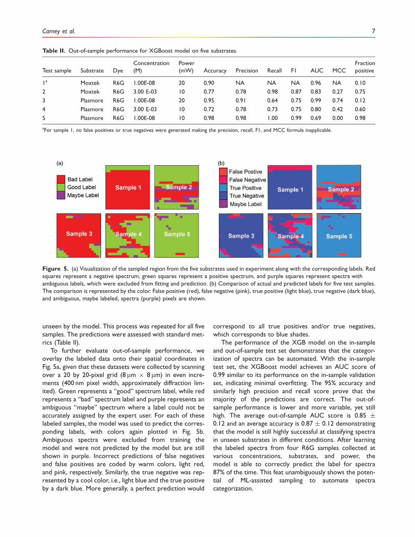
unseen by the model. This process was repeated for all five

samples. The predictions were assessed with standard met-

rics (Table II).

To further evaluate out-of-sample performance, we

overlay the labeled data onto their spatial coordinates in

Fig. 5a, given that these datasets were collected by scanning

over a 20 by 20-pixel grid (8 mm � 8 mm) in even incre-

ments (400 nm pixel width, approximately diffraction lim-

ited). Green represents a ‘‘good’’ spectrum label, while red

represents a ‘‘bad’’ spectrum label and purple represents an

ambiguous ‘‘maybe’’ spectrum where a label could not be

accurately assigned by the expert user. For each of these

labeled samples, the model was used to predict the corres-

ponding labels, with colors again plotted in Fig. 5b.

Ambiguous spectra were excluded from training the

model and were not predicted by the model but are still

shown in purple. Incorrect predictions of false negatives

and false positives are coded by warm colors, light red,

and pink, respectively. Similarly, the true negative was rep-

resented by a cool color, i.e., light blue and the true positive

by a dark blue. More generally, a perfect prediction would

correspond to all true positives and/or true negatives,

which corresponds to blue shades.

The performance of the XGB model on the in-sample

and out-of-sample test set demonstrates that the categor-

ization of spectra can be automated. With the in-sample

test set, the XGBoost model achieves an AUC score of

0.99 similar to its performance on the in-sample validation

set, indicating minimal overfitting. The 95% accuracy and

similarly high precision and recall score prove that the

majority of the predictions are correct. The out-of-

sample performance is lower and more variable, yet still

high. The average out-of-sample AUC score is 0.85 �

0.12 and an average accuracy is 0.87 � 0.12 demonstrating

that the model is still highly successful at classifying spectra

in unseen substrates in different conditions. After learning

the labeled spectra from four R6G samples collected at

various concentrations, substrates, and power, the

model is able to correctly predict the label for spectra

87% of the time. This feat unambiguously shows the poten-

tial of ML-assisted sampling to automate spectra

categorization.

Table II. Out-of-sample performance for XGBoost model on five substrates.

Test sample Substrate Dye

Concentration

(M)

Power

(mW) Accuracy Precision Recall F1 AUC MCC

Fraction

positive

1a Moxtek R6G 1.00E-08 20 0.90 NA NA NA 0.96 NA 0.10

2 Moxtek R6G 3.00 E-03 10 0.77 0.78 0.98 0.87 0.83 0.27 0.75

3 Plasmore R6G 1.00E-08 20 0.95 0.91 0.64 0.75 0.99 0.74 0.12

4 Plasmore R6G 3.00 E-03 10 0.72 0.78 0.73 0.75 0.80 0.42 0.60

5 Plasmore R6G 1.00E-08 10 0.98 0.98 1.00 0.99 0.69 0.00 0.98

aFor sample 1, no false positives or true negatives were generated making the precision, recall, F1, and MCC formula inapplicable.

Figure 5. (a) Visualization of the sampled region from the five substrates used in experiment along with the corresponding labels. Red

squares represent a negative spectrum, green squares represent a positive spectrum, and purple squares represent spectra with

ambiguous labels, which were excluded from fitting and prediction. (b) Comparison of actual and predicted labels for five test samples.

The comparison is represented by the color. False positive (red), false negative (pink), true positive (light blue), true negative (dark blue),

and ambiguous, maybe labeled, spectra (purple) pixels are shown.

Carney et al. 7

Discussion

Here we introduced ML-assisted SERS spectra classification

methodology to streamline acquisition and efficiently clas-

sify recorded spectra. The exclusion of negative signals

from the SERS analysis already takes place during normal

experimentation. When scanning a substrate, the majority

of signals are negative (e.g., noisy, not representative of the

typical sampled areas, out of focus, capture cosmic rays).

Typically, a trained experimentalist makes the determin-

ation of when a ‘‘good’’ signal is collected. Although sub-

jective, this strategy utilizes our impressive pattern

matching ability, which is challenging to replicate with struc-

tured algorithms. This technique excludes the majority of

negative spectra by avoiding their initial collection, but it is

not perfect and negative spectra occasionally creep into the

recorded dataset. Although experimentalists can easily dis-

tinguish between good and bad spectra, the large datasets

collected using typical SERS experiments make manual

excluding the negative spectra post-collection onerous. In

addition to presenting a barrier to large data set collection,

these expert user-driven decisions also limit the application

of SERS in a clinical setting. For SERS technology to transfer

from the research laboratory to the clinic, these subjective

labor intensive steps must be eliminated.

The scholarly literature encompassing automatization

endeavors of Raman and SERS measurements predomin-

antly demonstrates approaches to automate either (i) the

collection or (ii) the data preprocessing phase, e.g., baseline

correction, cosmic ray-induced spike removal, noise reduc-

tion, scaling and normalization, background subtraction,

including various thresholding techniques to harness

signal-to-noise ratio for spectra selection.2–4 The main limi-

tations of the current preprocessing techniques are that

they either rely on tuning the processing parameters (e.g.,

fitting parameters) or require calculating and thresholding

the S/N, which is not possible if the underlying analyte signal

is not known or highly fluctuating. Work by Dallaire et al.

discusses the importance of spectral quality for further

downstream analyses.46 In particular, they also note the

caveat in current literature reports; the spectral quality

assessment is largely made offline based on qualitative

visual inspection instead of using unbiased and systematic

quantitative criteria. The authors elaborately demonstrate

the effectiveness of excluding ‘‘bad’’ spectra in cancer

detection application.46 Therefore, there exists a clear

niche to design robust workflows to select spectra for

the downstream analyses. In essence, our strategy is inde-

pendent of the spectral preprocessing approaches and S/N

thresholding, rendering it a promising means to be applied

in a wide variety of different platforms.

The underlying reasons why a SERS spectrum may be

classified as ‘‘good’’ or ‘‘bad’’ are likely arising from either

(1) variations in local analyte concentration or (2) the SERS

hotspot phenomena, i.e., localized regions of extreme

electromagnetic fields that are highly dependent on under-

lying substrate geometry and analyte orientation.47–49 Even

at the single junction scale, hotspots are highly dynamic in

spatial dimension and in time,28 and thus majorly contribute

to the dynamic nature of the observed SERS signals. A per-

tinent yet rarely addressed phenomenon is the spot-to-

spot SERS reproducibility. Variation of EF across hotspots

is conventionally determined by the substrate uniformity,

i.e., the controlled sizes and spacings of the plasmonic fea-

tures, and also by the total number of hotspots in the

detection area. It is possible that this ML approach can

help in elucidating the characteristics of SERS hotspots as

well as the spectra variability. For example, ML methods can

be used for efficient SERS substrate development, since the

role of various physical and chemical parameters can be

systematically evaluated at the substrate engineering

phase. Essentially, our approach can be adapted to charac-

terize the signal-to-noise across a given sample and over

time. Until now this development and optimization has

traditionally been carried out by finite element modeling

(FEM), but the complementary ML approaches can greatly

contribute to these processes by allowing for rapid and

concise scrutiny of many spectra.

ML algorithms are able to codify human intuition by

learning from labeled training data and are well-suited to

identify noisy, feature-poor spectra. The use of a ML algo-

rithm has several advantages over a traditional structured

algorithm. A trained ML model requires no parameter

tuning once trained and can learn from the extensive

experience of trained experimentalists. With the availability

of open-source ML packages,42 training and integration are

straightforward. A plethora of different classes of ML algo-

rithms exist and new ones are frequently being invented. Of

the existing classes, they can roughly be divided into two

domains, classical ML algorithms and deep learning algo-

rithms. Classical ML algorithms include tree-based algo-

rithms such as random forest and XGBoost, as well as

more established classifiers like support vector machines.

Deep learning algorithms encompass the tremendous diver-

sity of multilayered neural network models, such as CNNs.

Both classical and deep learning models can achieve simi-

larly high performance, but classic ML algorithms can per-

form well on smaller datasets, whereas deep learning

architectures typically require tens of thousands of data

points to converge. In this current work, the complete

dataset consisted of only 2000 different spectra, thus the

tested models were confined to classical models, yet the

methods presented here are easily extendable to deep

learning models when working with larger datasets.

Amongst all the models tested here, the XGBoost

model performed best across both the in-sample and out-

of-sample datasets. Its performance in this dataset matches

our expectation that it is performing akin to a user expert

making an intuitive decision. To detail this, consider the

8 Applied Spectroscopy 0(0)

major inter-sample variation in the fraction of expert

assigned positive labels, likely due to the inhomogeneous

covering of dried R6G on the SERS substrates. In sample

one, 90% of the spectra are negatively labeled and the clas-

sifier predicts a negative label for all of them. In sample 5,

the reverse situation occurs; 98% of the spectra are posi-

tively labeled and the XGB model assigns a positive label to

all the spectra. In these extreme cases, XGB is essentially

learning from the out-of-sample labels and not taking into

consideration the unique characteristics of the substrate. In

this case, an expert experimentalist would adjust their own

threshold of classification based on the observed signal-to-

noise in a specified sample. For example, if many weak sig-

nals were observed, the threshold for collecting a spectrum

would be lower than in the case where the majority of

spectra had an apparent high signal-to-noise ratio. In the

intermediate case of sample 4 with a 60% positive rate, the

algorithm performs well (AUC ¼ 0.80), although lower

than in the test case (AUC ¼ 0.99). Nevertheless, the algo-

rithm is still successful in categorizing samples with a range

of positivity rates.

For the purpose of this study to develop versatile and

efficient ML-assisted tools for SERS spectra classification,

we chose a known chemical standard molecule R6G. This

model compound provided a combination of adequate

spectral complexity and variability (e.g., uneven distribution

of solution on the substrates resulting in varying degrees of

noise) to simulate a typical SERS experiment and subse-

quent spectra processing. Regarding broader generalizabil-

ity to more complex analytes such as biological matrices,

the best performing ML models (RF and XGBoost) in this

work are nonparametric models that do not make any

assumptions of the functional form of the classifier. This

flexibility ensures that the shape of the dividing lines

between the classes, i.e., hyperplanes, deployed by these

models can take arbitrary forms, contrasted to logistic

regression models where hyperplanes would be linear.

Thus, even complex spectra can be efficiently separated

from each other since the success of classification does

not depend on the complexity or level of noise in the spec-

tral data but instead on the experimentalist’s capability to

consistently label spectra as ‘‘good’’ or ‘‘bad’’, based on

their own interpretation of data quality, e.g., S/N or pres-

ence of trace element peaks.

Additionally, our analyses demonstrated that the ML

algorithm is robust at classifying out-of-sample spectra,

even across different substrates. However, this experiment

does not provide proof that the model is generalizable to all

situations, and users wishing to adopt this methodology

would need to train new models on a given substrate/ana-

lyte pair of interest using the Labeler app. In general, the

main limitation of the current approach will be the need to

re-train the ML models for varying instrument- and mea-

surement-related parameters. For example, it is likely that

the model is dependent on a given laser power, magnifica-

tion, and acquisition time. However, if experimental param-

eters are standardized, our out-of-sample performance

experiments suggest that inter-substrate and -sample per-

formance is stable. While here we tested highly ordered

SERS substrates, we expect that our ML classification

approach would perform equally well on SERS platforms

comprising nanoparticles in colloidal solutions, even

though they typically exhibit more geometrical and topo-

logical variation.1,50 Such nanoparticle-based SERS experi-

ments are typically carried out either directly in colloidal

solutions or after nanoparticles precipitate or self-assemble

on supports. This ultimately leads to a ‘‘metastable’’ envir-

onment, especially for colloidal solutions that are highly

dynamic. Yet the optical near-field signal amplification is

dependent on the local plasmonic field at any given point

in the sample, thus we expect individual spectra to still be

produced that can be classified as ‘‘bad’’ or ‘‘good’’. As long

as the experimentalist can carry out concise pre-classifica-

tion and model training with the Labeler app, the classifica-

tion performance is conserved despite the geometry or

constituent properties of the underlying substrate.

Future work using this approach will involve automatically

tuning the classification threshold based on the number of

positively classified spectra in a sample. We also will explore

the feedback of this trained algorithm to control stage move-

ment and automate measurement of full datasets.

Conclusion

This work describes application of an ML algorithm to

address a central challenge for adapting SERS to automated

platforms: the current dependency of expert user-driven

endpoints for sampling. The elimination of bad spectra

from a collected dataset can increase the signal-to-noise

ratio by reducing the variance. Especially in SERS applica-

tions, it is desired to collect and analyze as homogeneous

sets of spectra as possible, which is accomplished by the ML-

assisted spectra selection. By applying this algorithm to the

acquisition stage, the labor required to collect many spectra

can be reduced making collecting larger and more compre-

hensive datasets feasible. Furthermore, by automating the

acquisition stage of the SERS experiment, another barrier to

the clinical application of this technology can be broken

down. Given the exponential growth of acquired data (e.g.,

spectra, images, or videos), there is an immense demand for

integrating reliable, automated, and fast analysis methods to

the experimental procedures for SERS instrumentation. We

envision that the workflow described here will allow for

more robust automated SERS analyses. We foresee that

the introduced platform can be further expanded to quan-

titative analyses of chemicals as well as complex biological

and clinical samples such as patient-derived EVs or crude

serum for modern diagnostic purposes.

Carney et al. 9

Declaration of Conflicting Interests

The author(s) declared no potential conflicts of interest with

respect to the research, authorship, and/or publication of this

article.

Funding

This work was supported by the UC Davis Center for Data

Science and Artificial Intelligence Research (CeDAR) Innovative

Data Science Seed Funding Program; the Ovarian Cancer

Education and Research Network, Inc. (OCERN); the NIH/NCI

[R01CA241666]. The ThermoFisher Quattro ESEM was funded

through the US National Science Foundation under award DMR-

1725618.

Data Accessibility Statement

All data collected for this study, including SERS datasets and the

Labeler program files, can be downloaded from the following open

repository: https://doi.org/10.5281/zenodo.3994784. All open-

source Python code will be maintained at: https://www.github.

com/kul-group/ramanbox.

Supplemental Material

All supplemental material mentioned in the text is available in the

online version of the journal.

ORCID iDs

Dexter Antonio https://orcid.org/0000-0001-7181-8270

Randy P. Carney https://orcid.org/0000-0001-8193-1664

References

1. J. Langer, D.J. de Aberasturi, J. Aizpurua, R.A. Alvarez-Puebla, et al.

‘‘Present and Future of Surface-Enhanced Raman Scattering’’. ACS

Nano. 2020. 14(1): 28–117. doi: 10.1021/acsnano.9b04224.

2. F.W.L. Esmonde-White, M.V. Schulmerich, K.A. Esmonde-White,

M.D. Morris. ‘‘Automated Raman Spectral Preprocessing of Bone and

Other Musculoskeletal Tissues’’. Proc. SPIE. Int. Soc. Opt. Eng. 2009.

7166: 716605. doi: 10.1117/12.809436.

3. G. Lopez-Reyes, F.R. Perez. ‘‘A Method for the Automated Raman

Spectra Acquisition’’. J. Raman Spectrosc. 2017. 48(11): 1654–1664.

doi: 10.1002/jrs.5185.

4. H.G. Schulze, S. Rangan, J.M. Piret, M.W. Blades, et al. ‘‘Developing Fully

Automated Quality Control Methods for Preprocessing Raman Spectra

of Biomedical and Biological Samples’’. Appl. Spectrosc. 2018. 72(9):

1322–1340. doi: 10.1177/0003702818778031.

5. W. Hu, S. Ye, Y. Zhang, T. Li, et al. ‘‘Machine Learning Protocol for

Surface-Enhanced Raman Spectroscopy’’. J. Phys. Chem. Lett. 2019.

10(20): 6026–6031. doi: 10.1021/acs.jpclett.9b02517.

6. X. Fan, W. Ming, H. Zeng, Z. Zhang, et al. ‘‘Deep Learning-Based

Component Identification for the Raman Spectra of Mixtures’’.

Analyst. 2019. 144(5): 1789–1798. doi: 10.1039/C8AN02212G.

7. J. Liu, M. Osadchy, L. Ashton, M. Foster, et al. ‘‘Deep Convolutional

Neural Networks for Raman Spectrum Recognition: A Unified

Solution’’. Analyst. 2017. 142(21): 4067–4074. doi: 10.1039/

C7AN01371J.

8. A.A. Moawad, A. Silge, T. Bocklitz, K. Fischer, et al. ‘‘Machine Learning-

Based Raman Spectroscopic Assay for the Identification of Burkholderia

Mallei and Related Species’’. Molecules. 2019. 24(24): 4516. doi:

10.3390/molecules24244516.

9. R.M. Jarvis, R. Goodacre. ‘‘Discrimination of Bacteria Using Surface-

Enhanced Raman Spectroscopy’’. Anal. Chem. 2004. 76(1): 40–47. doi:

10.1021/ac034689c.

10. B. Deng, X. Luo, M. Zhang, L. Ye, et al. ‘‘Quantitative Detection of

Acyclovir by Surface Enhanced Raman Spectroscopy Using a Portable

Raman Spectrometer Coupled with Multivariate Data Analysis’’.

Colloids Surf., B. 2019. 173: 286–294. doi: 10.1016/

j.colsurfb.2018.09.058.

11. S.-X. Li, Q.-Y. Zeng, L.-F. Li, Y.-J. Zhang, et al. ‘‘Study of Support Vector

Machine and Serum Surface-Enhanced Raman Spectroscopy for

Noninvasive Esophageal Cancer Detection’’. J. Biomed. Opt. 2013.

18(2): 27008. doi: 10.1117/1.JBO.18.2.027008.

12. Y. Zhang, X. Ye, G. Xu, X. Jin, et al. ‘‘Identification and Distinction of

Non-Small-Cell Lung Cancer Cells by Intracellular SERS Nanoprobes’’.

RSC Adv. 2016. 6(7): 5401–5407. doi: 10.1039/C5RA21758J.

13. Y. Yu, Y. Lin, C. Xu, K. Lin, et al. ‘‘Label-free detection of nasophar-

yngeal and liver cancer using surface-enhanced Raman spectroscopy

and partial lease squares combined with support vector machine’’.

Biomed. Opt. Express. 2018. 9(12): 6053–6066. doi: 10.1364/

BOE.9.006053.

14. W. Lee, A.T.M. Lenferink, C. Otto, H.L. Offerhaus. ‘‘Classifying Raman

Spectra of Extracellular Vesicles Based on Convolutional Neural

Networks for Prostate Cancer Detection’’. J. Raman Spectrosc.

2020. 51(2): 293–300. doi: 10.1002/jrs.5770.

15. J. Park, M. Hwang, B. Choi, H. Jeong, et al. ‘‘Exosome Classification by

Pattern Analysis of Surface-Enhanced Raman Spectroscopy Data for

Lung Cancer Diagnosis’’. Anal. Chem. 2017. 89(12): 6695–6701. doi:

10.1021/acs.analchem.7b00911.

16. J. Carmicheal, C. Hayashi, X. Huang, L. Liu, et al. ‘‘Label-Free

Characterization of Exosome Via Surface Enhanced Raman

Spectroscopy for the Early Detection of Pancreatic Cancer’’.

Nanomedicine. 2019. 16: 88–96. doi: 10.1016/j.nano.2018.11.008.

17. N. Banaei, J. Moshfegh, A. Mohseni-Kabir, J.M. Houghton, et al.

‘‘Machine Learning Algorithms Enhance the Specificity of Cancer

Biomarker Detection Using SERS-Based Immunoassays in

Microfluidic Chips’’. RSC Adv. 2019. 9(4): 1859–1868. doi: 10.1039/

C8RA08930B.

18. E. Guevara, J.C. Torres-Galvan, M.G. Ramırez-Elıas, C. Luevano-

Contreras, et al. ‘‘Use of Raman Spectroscopy to Screen Diabetes

Mellitus with Machine Learning Tools’’. Biomed. Opt. Express. 2018.

9(10): 4998–5010. doi: 10.1364/BOE.10.004489.

19. S.D. Krauß, R. Roy, H.K. Yosef, T. Lechtonen, et al. ‘‘Hierarchical Deep

Convolutional Neural Networks Combine Spectral and Spatial

Information for Highly Accurate Raman-Microscopy-Based

Cytopathology’’. J. Biophotonics. 2018. 11(10): e201800022. doi:

10.1002/jbio.201800022.

20. H. Shi, H. Wang, X. Meng, R. Chen, et al. ‘‘Setting Up a Surface-

Enhanced Raman Scattering Database for Artificial-Intelligence-Based

Label-Free Discrimination of Tumor Suppressor Genes’’. Anal. Chem.

2018. 90(24): 14216–14221. doi: 10.1021/acs.analchem.8b03080.

21. I.J. Hidi, M. Jahn, K. Weber, T. Bocklitz, et al. ‘‘Lab-on-a-Chip-Surface

Enhanced Raman Scattering Combined with the Standard Addition

Method: Toward the Quantification of Nitroxoline in Spiked Human

Urine Samples’’. Anal. Chem. 2016. 88(18): 9173–9180. doi: 10.1021/

acs.analchem.6b02316.

22. O. Alharbi, Y. Xu, R. Goodacre. ‘‘Simultaneous Multiplexed

Quantification of Caffeine and its Major Metabolites Theobromine

and Paraxanthine Using Surface-Enhanced Raman Scattering’’. Anal.

Bioanal. Chem. 2015. 407(27): 8253–8261. doi: 10.1007/s00216-015-

9004-8.

23. S.M. Moosavi, A. Chidambaram, L. Talirz, M. Haranczyk, et al.

‘‘Capturing Chemical Intuition in Synthesis of Metal-Organic

Frameworks’’. Nat. Commun. 2019. 10(1): 539. doi: 10.1038/

s41467-019-08483-9.

24. D. Shen, G. Wu, H.-I. Suk. ‘‘Deep Learning in Medical Image Analysis’’.

Annu. Rev. Biomed. Eng. 2017. 19(1): 221–248. doi: 10.1146/annurev-

bioeng-071516-044442.

25. D.L. Jeanmaire, R.P. Van Duyne. ‘‘Surface Raman

Spectroelectrochemistry: Part I. Heterocyclic, Aromatic, and

10 Applied Spectroscopy 0(0)

Aliphatic Amines Adsorbed on the Anodized Silver Electrode’’.

J. Electroanal. Chem. Interfacial Electrochem. 1977. 84(1): 1–20. doi:

10.1016/S0022-0728(77)80224-6.

26. M. Fleischmann, P.J. Hendra, A.J. McQuillan. ‘‘Raman Spectra of

Pyridine Adsorbed at a Silver Electrode’’. Chem. Phys. Lett. 1974.

26(2): 163–166. doi: 10.1016/0009-2614(74)85388-1.

27. M.G. Albrecht, J.A. Creighton. ‘‘Anomalously Intense Raman Spectra

of Pyridine at a Silver Electrode’’. J. Am. Chem. Soc. 1977. 99(15):

5215–5217. doi: 10.1021/ja00457a071.

28. A.M. Michaels, J. Jiang, L. Brus. ‘‘Ag Nanocrystal Junctions as the Site

for Surface-Enhanced Raman Scattering of Single Rhodamine 6G

Molecules’’. J. Phys. Chem. B. 2000. 104(50): 11965–11971. doi:

10.1021/jp0025476.

29. X. Xu, K. Kim, H. Li, D.L. Fan. ‘‘Ordered Arrays of Raman

Nanosensors for Ultrasensitive and Location Predictable

Biochemical Detection’’. Adv. Mater. 2012. 24: 5457–5463. doi:

10.1002/adma.201201820.

30. B. Vincent, J. Edwards, S. Emmett, A. Jones. ‘‘Depletion Flocculation in

Dispersions of Sterically-Stabilised Particles (‘‘Soft Spheres’’)’’.

Colloids Surf. 1986. 18(2): 261–281. doi: 10.1016/0166-

6622(86)80317-1.

31. L.A. Wijenayaka, M.R. Ivanov, C.M. Cheatum, A.J. Haes. ‘‘Improved

Parametrization for Extended Derjaguin, Landau, Verwey, and

Overbeek Predictions of Functionalized Gold Nanosphere Stability’’.

J. Phys. Chem. C. 2015. 119(18): 10064–10075. doi: 10.1021/

acs.jpcc.5b00483.

32. S.R. Saunders, M.R. Eden, C.B. Roberts. ‘‘Modeling the Precipitation of

Polydisperse Nanoparticles Using a Total Interaction Energy Model’’. J.

Phys. Chem. C. 2011. 115(11): 4603–4610. doi: 10.1021/jp200116a.

33. L.M. Almehmadi, S.M. Curley, N.A. Tokranova, S.A. Tenenbaum, et al.

‘‘Surface Enhanced Raman Spectroscopy for Single Molecule Protein

Detection. Sci. Rep. 2019. 9(1): 12356. doi: 10.1038/s41598-019-

48650-y.

34. K.A. Bosnick, Jiang, L.E. Brus. ‘‘Fluctuations and Local Symmetry in

Single-Molecule Rhodamine 6G Raman Scattering on Silver

Nanocrystal Aggregates’’. J. Phys. Chem. B. 2002. 106(33):

8096–8099. doi: 10.1021/jp0256241.

35. A.B. Zrimsek, N. Chiang, M. Mattei, S. Zaleski, et al. ‘‘Single-Molecule

Chemistry with Surface- and Tip-Enhanced Raman Spectroscopy’’.

Chem. Rev. 2017. 117(11): 7583–7613. doi: 10.1021/

acs.chemrev.6b00552.

36. E.C.L. Ru, P.G. Etchegoin. ‘‘Single-Molecule Surface-Enhanced Raman

Spectroscopy’’. Annu. Rev. Phys. Chem. 2012. 63(1): 65–87. doi:

10.1146/annurev-physchem-032511-143757.

37. A. Szeghalmi, S. Kaminskyj, P. Rosch, J. Popp, et al. ‘‘Time Fluctuations

and Imaging in the SERS Spectra of Fungal Hypha Grown on

Nanostructured Substrates’’. J. Phys. Chem. B. 2007. 111(44):

12916–24. doi: 10.1021/jp075422a.

38. J. Taylor, A. Huefner, L. Li, J. Wingfield, et al. ‘‘Nanoparticles

and Intracellular Applications of Surface-Enhanced Raman

Spectroscopy’’. Analyst. 2016. 141(17): 5037–5055. doi: 10.1039/

C6AN01003B.

39. Unidata. netCDF4 Version 1.5.6. Boulder, CO: UCAR/Unidata, 2021.

doi: 10.5065/D6H70CW6.

40. Z.-M. Zhang, S. Chen, Y.-Z. Liang. ‘‘Baseline Correction Using

Adaptive Iteratively Reweighted Penalized Least Squares’’. Analyst.

2010. 135(5): 1138–1146. doi: 10.1039/b922045c.

41. P.H.C. Eilers. ‘‘A Perfect Smoother’’. Anal. Chem. 2003. 75(14):

3631–3636. doi: 10.1021/ac034173t.

42. F. Pedregosa, G. Varoquaux, A. Gramfort, V. Michel, et al. ‘‘Scikit-

Learn: Machine Learning in Python’’. J. Mach. Learn. Res. 2011. 12:

2825–2830.

43. T. Chen, C. Guestrin. ‘‘XGBoost: A Scalable Tree Boosting System’’. In

Proceedings of the 22nd ACM SIGKDD International Conference on

Knowledge Discovery and Data Mining, Association for Computing

Machinery, San Francisco, CA: August 13, 2016, 2016. Pp. 785–794.

doi: 10.1145/2939672.2939785.

44. T.A. Lasko, J.G. Bhagwat, K.H. Zou, L. Ohno-Machado. ‘‘The Use of

Receiver Operating Characteristic Curves in Biomedical Informatics’’.

J. Biomed. Inf. 2005. 38(5): 404–415. doi: 10.1016/j.jbi.2005.02.008.

45. S.M. Borstelmann. ‘‘Machine Learning Principles for Radiology

Investigators’’. Acad. Radiol. 2020. 27(1): 13–25. doi: 10.1016/

j.acra.2019.07.030.

46. F. Dallaire, F. Picot, J.-P. Tremblay, G. Sheehy, et al. ‘‘Quantitative

Spectral Quality Assessment Technique Validated Using

Intraoperative In Vivo Raman Spectroscopy Measurements. J.

Biomed. Opt. 2020. 25(4): 040501. doi: 10.1117/1.JBO.25.4.040501.

47. J.A. Creighton, C.G. Blatchford, M.G. Albrecht. ‘‘Plasma Resonance

Enhancement of Raman Scattering by Pyridine Adsorbed on Silver or

Gold Sol Particles of Size Comparable to the Excitation Wavelength’’.

J. Chem. Soc., Faraday Trans. 2. 1979. 75: 790–798. doi: 10.1039/

F29797500790.

48. H. Cang, A. Labno, C. Lu, X. Yin, et al. ‘‘Probing the Electromagnetic

Field of a 15-Nanometre Hotspot by Single Molecule Imaging’’.

Nature. 2011. 469: 385–388. doi: 10.1038/nature09698.

49. D. Radziuk, H. Moehwald. ‘‘Prospects for Plasmonic Hot Spots in

Single Molecule SERS Towards the Chemical Imaging of Live Cells’’.

Phys. Chem. Chem. Phys. 2015. 17: 21072–21093. doi: 10.1039/

C4CP04946B.

50. D.M. Solıs, J.M. Taboada, F. Obelleiro, L.M. Liz-Marzan, et al.

‘‘Optimization of Nanoparticle-Based SERS Substrates Through

Large-Scale Realistic Simulations’’. ACS Photonics. 2017. 4(2):

329–337. doi: 10.1021/acsphotonics.6b00786.

Carney et al. 11