CDMTCS

Research

Report

Series

Construmath South 2012

Applications of Non-Classical

Logic

Proceedings of the Workshop

at Westport

Maarten McKubre-Jordens,

Raazesh Sainudiin (Eds.)

University of Canterbury, NZ

CDMTCS-420

19 April 2012

Centre for Discrete Mathematics and

Theoretical Computer Science

Construmath South 2012

Applications of Non-Classical Logic

Proceedings of the Workshop at Westport

26–28 January 2012

Maarten McKubre-Jordens & Raazesh Sainudiin (Eds.)

This meeting was supported by Marie Curie grant PIRSES-GA-2008-230822 from the European Union,

with counterpart funding from the Ministry of Research, Science and Technology of New Zealand, for

the project Construmath. Additional financial and infrastructure support was generously provided by

the University of Canterbury.

Co-Organizers of Construmath South 2012

Maarten McKubre-Jordens & Raazesh Sainudiin

Proceedings Compiled by

Maarten McKubre-Jordens & Raazesh Sainudiin

Administrative Support

Penelope Goode

Technical Support

Steve Gourdie

Copyright c� 2012

The copyright of any material in this booklet (including without limitation the text, computer code, artwork,

photographs, and images) is owned by the respective authors and/or the editors. You may request permission to

use the copyright materials in this booklet by contacting the respective authors and/or the editors.

Foreword

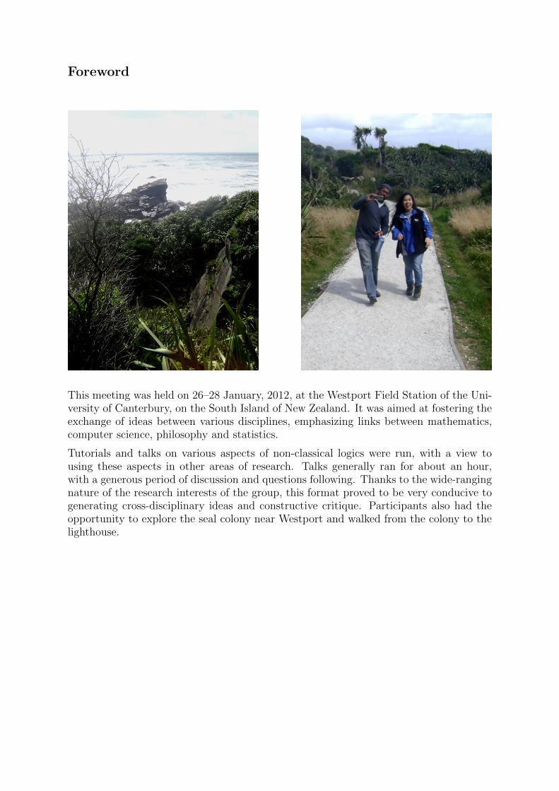
This meeting was held on 26–28 January, 2012, at the Westport Field Station of the Uni-versity of Canterbury, on the South Island of New Zealand. It was aimed at fostering theexchange of ideas between various disciplines, emphasizing links between mathematics,computer science, philosophy and statistics.

Tutorials and talks on various aspects of non-classical logics were run, with a view tousing these aspects in other areas of research. Talks generally ran for about an hour,with a generous period of discussion and questions following. Thanks to the wide-rangingnature of the research interests of the group, this format proved to be very conducive togenerating cross-disciplinary ideas and constructive critique. Participants also had theopportunity to explore the seal colony near Westport and walked from the colony to thelighthouse.

Participants ofConstruMath South 2012: Applications of Non-Classical Logic

and Their Double Pendulum Release Signatures

The participants from left to right in the first image are: Ruriko Yoshida, Cris Calude,Raazesh Sainudiin, Maarten McKubre-Jordens, Elena Calude, Nicholas Duncan, JamesDent, Ty Baen, Zach Weber, Ed Mares and Bruce Burdick. Each participant released amechatronically measurable double pendulum. The remaining eleven images (from leftto right and row by row) show the positions of each arm of the double pendulum throughtime upon release by each participant in the above list order.

Contents

Parameter Estimation in Epistemologically Valid Machine Interval Exper-imentsRaazesh Sainudiin (with Alex Danis and Warwick Tucker)University of Canterbury 1

What’s the Deal with Relevance?An Introduction to Relevant LogicEdwin MaresVictoria University of Wellington 6

Paraconsistent MathematicsZach WeberUniversity of Otago 17

Constructive Methods in MathematicsMaarten McKubre-JordensUniversity of Canterbury 19

A Constructive Approach to the Complexity of Mathematical ProblemsCristian Calude and Elena CaludeUniversity of Auckland / Massey University 21

Abstract Stone Duality - A Logic for TopologyNicholas DuncanUniversity of Canterbury 27

Epistemolog

ically

valid

experim

ent

Outline

Statemen

t(H

ume,

1777

)

“Butwheredi↵eren

te↵

ects

have

beenfoundto

follow

from

causes,

whichareto

appearance

exactly

similar,allthesevariouse↵

ects

must

occurto

themindin

transferringthepast

tothefuture,anden

terinto

ourco

nsideration,when

we

determinetheprobabilityoftheeven

t.”[1]

Epistem

ologically

valid

experim

ent

Datafrom

ado

uble

pendu

lum

Mod

elwithparameter

space⇥⇥

(Rk,k

<1

Actionspaceof

point

estimationA

=⇥⇥

Solution

MLEisCSPwithepistemolog

ically

valid

action

spaceI⇥⇥

⇤

Set-valuedintegrators,(T

,F,?)-basedestimators

Blabb

eron

Ong

oing

Work

A.Dan

is,R.Sainudiin

&W

.Tucker

MLEof

amachineinterval

experim

ent

Epistemolog

ically

valid

experim

ent

Lim

itson

Numerical

resolution

(LNR)

Lim

itson

Empirical

Resolution

Lim

itson

Empirical

Resolution

Epistem

ologically

valid

experim

ent

Definition

Epistemologyisthestud

yof

thenature

andgrou

ndsof

know

ledg

eespecially

withreferenceto

itslim

itsandvalidity.

Definition

Astatistica

lex

perim

entE P

isthetriple

(X,F

X,P

)consisting

ofasamplespaceX

ofallpossibleem

pirically

observable

realizations

ofanaturalph

enom

enon

�,asigm

a-algebraFXon

X,anda

family

ofprob

ability

measuresP

={P

✓,✓

2⇥},

where

each

P

✓is

aprob

ability

measure

onthemeasurablespace(X

,FX).

The

✓is

anindexbelon

ging

totheindexset⇥.The

indexmap

d(✓)=

P

✓:⇥!P

associates

every✓2⇥

withP

✓2P,in

anarbitrarymannerthat

even

allowsfortheindexmap

dto

bethe

identity

map

with⇥

=P.

A.Dan

is,R.Sainudiin

&W

.Tucker

MLEof

amachineinterval

experim

ent

Epistemolog

ically

valid

experim

ent

Param

eter

Estim

ationin

Epistem

ologically

valid

Machine

Interval

Experim

ents

Raazesh

Sainu

diin

Departm

entof

MathematicsandStatistics,

Universityof

Canterbury,Private

Bag

4800

,

Christchu

rch,

New

Zealand

jointworkwith

Alexand

erDanisandWarwickTucker

Departm

entof

Mathematics,

Upp

sala

University,Box

480Upp

sala,Sweden

Con

struMathSou

th2012,Westport,New

Zealand

Janu

ary26-28,

2011

A.Dan

is,R.Sainudiin

&W

.Tucker

MLEof

amachineinterval

experim

ent

Epistemolog

ically

valid

experim

ent

The

DualisticContext

(“The

BiggerPicture”)

Tradition:Mod

ernEurop

eanEmpiricism

Internal

Consisten

cy:AristoteleanLogic

Universe

ofHyp

otheses:Pop

per’sFalsifia

bility

Empirical

Resolution:Mechatron

ically

MeasuredDataD

o

Model

:DeterministicODE-IVPs

Param

eter

Spac

e:fin

itedimension

alparameter

space

Approac

h:Statistical

DecisionTheory(set-valuedapproach)

Enginee

ringConstraints:Resou

rce-lim

ited

Info.Proc.

Objective:Epistem

ologically

Valid

Param

eter

Estim

ation

Solution:Com

puter-aidedProofs&

Interval

Analysis

A.Dan

is,R.Sainudiin

&W

.Tucker

MLEof

amachineinterval

experim

ent

1

Epistemolog

ically

valid

experim

ent

Lim

itson

Numerical

resolution

(LNR)

Lim

itson

Empirical

Resolution

Lim

itson

Empirical

Resolution

ODEModel:Dam

ped

SinglePendu

lum

Trajectories

Kinetic

energy

ofthearm

consistsof

only

rotation

alkinetic

energy

T=

1 2I'

2,

Thepoten

tial

energy

ofthepen

dulum

iscalculatedby

consideringthege

ometric

positionof

thecentreof

massab

ovetheeq

uilibrium

position,V

=ml cg(1

�co

s')

Lag

rangian

ofthesinglepen

dulum:

L=

T�

V(1)

=1 2I'

2�

ml cg(1

�co

s').

(2)

TheEuler-Lag

range

form

:d

dt

✓@L

@'

◆�

@L

@'

=0,

(3)

givingtheeq

uationof

motionforthesinglepen

dulum

system

,

I'+

mgl csin'=

0(4)

or,

'=

�⇠2sin'

(5)

where⇠=

qml cg

I.

A.Dan

is,R.Sainudiin

&W

.Tucker

MLEof

amachineinterval

experim

ent

Epistemolog

ically

valid

experim

ent

Lim

itson

Numerical

resolution

(LNR)

Lim

itson

Empirical

Resolution

Lim

itson

Empirical

Resolution

ODEModel:Dam

ped

SinglePendu

lum

Trajectories

Tonumerically

integratetheeq

uationof

motion,weco

nvert

(5)into

asystem

offirst

order

equationsby

letting'=

!an

ddi↵eren

tiating,

!=

'.Thuswehavethesystem

offirstorder

equations,

' !

�=

!

�⇠2sin'

�(6)

Frictionmay

bead

ded

tothesystem

byad

dingan

other

term

to(4).

Thefriction

inthis

case

ismodeled

asprop

ortion

alto

thean

gularvelocity,thetorqueproducedis

givenby,

⌧ b=

µ'

giving(4)as,

I'+

µ'+

mgl csin'=

0(7)

A.Dan

is,R.Sainudiin

&W

.Tucker

MLEof

amachineinterval

experim

ent

Epistemolog

ically

valid

experim

ent

Lim

itson

Numerical

resolution

(LNR)

Lim

itson

Empirical

Resolution

Lim

itson

Empirical

Resolution

Phenomenon:Dam

ped

DoublePendu

lum

Trajectories

A:DPSchem

atic

B:StreamingDPdata

C:Enclosuresof

twoinitially

closetrajectories

A.Dan

is,R.Sainudiin

&W

.Tucker

MLEof

amachineinterval

experim

ent

Epistemolog

ically

valid

experim

ent

Lim

itson

Numerical

resolution

(LNR)

Lim

itson

Empirical

Resolution

Lim

itson

Empirical

Resolution

ODEModel:Dam

ped

SinglePendu

lum

Trajectories

ϕ

cl

Mod

elthearm

asadistribu

tedmasswithcentre

ofmass

locatedat

adistance

l

cfrom

thepivot,

mom

entof

inertiathearm

isIanditsmassism.

theacceleration

dueto

gravityisg⇡

9.81ms�

2,

'istheangu

larposition,

'istheangu

larvelocity,

A.Dan

is,R.Sainudiin

&W

.Tucker

MLEof

amachineinterval

experim

ent

2

Epistemolog

ically

valid

experim

ent

Lim

itson

Numerical

resolution

(LNR)

Lim

itson

Empirical

Resolution

Lim

itson

Empirical

Resolution

ODEModel:Passive

DoublePendu

lum

Trajectories

ϕ

ω

l 3

l 1

l 2

thecentre

ofmassof

theinnerarm

isdistance

l

1

thedistance

betweenpivots

oftheinnerarm

isl

3

thecentre

ofmassof

theou

terarm

isdistance

l

2

toparm

hasmassm

1andmom

entof

inertiaof

I 1similarlyfortheou

terarm

they

arem

2andI 2

A.Dan

is,R.Sainudiin

&W

.Tucker

MLEof

amachineinterval

experim

ent

Epistemolog

ically

valid

experim

ent

Lim

itson

Numerical

resolution

(LNR)

Lim

itson

Empirical

Resolution

Lim

itson

Empirical

Resolution

ODEModel:Passive

DoublePendu

lum

Trajectories

After

somework...

Derivationof

equationsviatheEuler-Lag

range

equationsof

motionfollo

wsin

anman

ner

analog

ousto

that

presen

tedforthepassive

singlepen

dulum...

Wecanthis

param

etricfamily

ofvector

fieldsforou

rstatisticalexperim

entwithdata

{x(t

i)} t

i2Tas

follo

ws: ⇥⇥3

✓,

x(t)=

Zf(x

⇤⇤⇤⇤⇤⇤⇤⇤⇤⇤⇤⇤;

✓)

Here,

x iis

asample

timean

dy i

=('

1,'

2)givesthean

gularpositionsof

each

arm

at

timex i

A.Dan

is,R.Sainudiin

&W

.Tucker

MLEof

amachineinterval

experim

ent

Epistemolog

ically

valid

experim

ent

Lim

itson

Numerical

resolution

(LNR)

Lim

itson

Empirical

Resolution

Lim

itson

Empirical

Resolution

Num

erical

Errorsdu

eto

LNR

Overflow

Error

(12!

=479001600,13!6=

1932053504)

Rou

ndingError

(actualresult-compu

tedresult)

Cancellation

Error

(accum

ulated

roun

d-o↵

error)

TruncationError

(from

doingon

lyfin

itelymanyop

erations)

Con

versionError

(decim

alto

finitesetof

binary

numbers)

Heuristic

punctual

localop

timizationisno

trigorous!

-0.2

-0.1

00.1

0.2

0

0.05

0.1

0.15

0.2

-1

01

23

45

6

-4

-3

-2

-1012

A.Dan

is,R.Sainudiin

&W

.Tucker

MLEof

amachineinterval

experim

ent

Epistemolog

ically

valid

experim

ent

Lim

itson

Numerical

resolution

(LNR)

Lim

itson

Empirical

Resolution

Lim

itson

Empirical

Resolution

Lim

itson

EmpiricalResolution

Inorderto

makethegrou

ndof

know

ledg

eab

out�

withLER

epistemologically

soun

d,theem

pirically

indiscerniblesets

mustbe

allowed

toenterthestatisticalexperim

entas

data.

A.Dan

is,R.Sainudiin

&W

.Tucker

MLEof

amachineinterval

experim

ent

3

Epistemolog

ically

valid

experim

ent

Lim

itson

Numerical

resolution

(LNR)

Lim

itson

Empirical

Resolution

Lim

itson

Empirical

Resolution

Epistem

ologically

valid

experim

ent

Definition

Epistemologyisthestud

yof

thenature

andgrou

ndsof

know

ledg

eespecially

withreferenceto

itslim

itsandvalidity.

Epistem

ological

Con

sideration

s:

Lim

itson

Num

erical

Resolution

Lim

itson

EmpiricalResolution

Lim

itson

Lingu

isticResolution(futurework!)

Lim

itson

...

A.Dan

is,R.Sainudiin

&W

.Tucker

MLEof

amachineinterval

experim

ent

Epistemolog

ically

valid

experim

ent

Lim

itson

Numerical

resolution

(LNR)

Lim

itson

Empirical

Resolution

Lim

itson

Empirical

Resolution

Lim

itson

Num

erical

resolution

(LNR)

Com

puters

supp

ortafin

itesetof

fixed

leng

thflo

ating-point

numbersof

theform

x=

±m

·be=

±0.m

1m

2···m

p·b

e

where,m

isthesign

edmantissaof

precisionp,bisthebase

(usually

2)ande,bou

nded

betweeneande,istheexpon

ent.

Whenb=

2,thedigits

ofthemantissam

1=

1and

m

i2{0,1},8i,1

<i

p[3].

A.Dan

is,R.Sainudiin

&W

.Tucker

MLEof

amachineinterval

experim

ent

Epistemolog

ically

valid

experim

ent

Lim

itson

Numerical

resolution

(LNR)

Lim

itson

Empirical

Resolution

Lim

itson

Empirical

Resolution

Epistem

ologically

Valid

Experim

ent

Wewantan

epistemologically

valid

experim

entthat

accoun

tsfortheph

ysical

limitson

empiricalresolution

(“show

whatyoucanactually

see”)

numerical

resolution

(“compu

tewhatyouactually

can”

)

A.Dan

is,R.Sainudiin

&W

.Tucker

MLEof

amachineinterval

experim

ent

Epistemolog

ically

valid

experim

ent

Lim

itson

Numerical

resolution

(LNR)

Lim

itson

Empirical

Resolution

Lim

itson

Empirical

Resolution

Solution ActionSpace

Aof

theclassicalestimationprob

lem

ismerely

theparameter

space⇥⇥

Epistem

ologically

valid

action

spaceAA

isa

machine-representable

Hausdor↵-extension

theParam

eter

Space

⇥⇥EN

�!I⇥⇥

⇤:=

I⇥⇥[;

I⇥⇥isthesetof

allcompact

boxes

in⇥⇥.

;hasto

beaddedto

ourepistemologically

valid

AAidentifia

bilityof

theextend

edexperim

entindexedby

I⇥⇥in

term

sof

symmetricsetdi↵erence

followsfrom

identifia

bilityof

theoriginal

experim

entindexedby

⇥⇥andinclusionmon

oton

yof

theindexmap

(likelihoo

dor

cond

itionalprob

ability

ofdata

givenparameter)

A.Dan

is,R.Sainudiin

&W

.Tucker

MLEof

amachineinterval

experim

ent

4

Epistemolog

ically

valid

experim

ent

Lim

itson

Numerical

resolution

(LNR)

Lim

itson

Empirical

Resolution

Lim

itson

Empirical

Resolution

Data

lossless

compression

(minim

alsu�cientstatistic)

ofthe

trajectory

themeasurablediscrete

statetransition

salon

gwiththe

transition

time

timestam

ps,arm-positionstates

areintegers

representing

intervals

sample

number,en

coder1,

enco

der2

2600

1042

-10

1578

-1-1

6752

-2-1

. . . 1222

243-2

2048

012

2933

0-1

2048

0

A.Dan

is,R.Sainudiin

&W

.Tucker

MLEof

amachineinterval

experim

ent

Epistemolog

ically

valid

experim

ent

Lim

itson

Numerical

resolution

(LNR)

Lim

itson

Empirical

Resolution

Lim

itson

Empirical

Resolution

Lim

itson

EmpiricalResolution

Wordsof

Vladik

Kreinov

ich(tworecentLos

Alamos

Rep

orts

onMeauremen

tErrors)

Inman

ysuch

situations,

theon

lythingwekn

owis

theupper

bou

nddon

the

measuremen

terror.

Thus,

afterwege

tthemeasuredva

lueX,theon

lyinform

ation

that

wehav

eab

outtheactual

(unkn

own)va

luexis

that

xbelon

gsto

theinterval

[X�

d,X

+d].

Here,

wehav

etw

och

oices:

(a)

wecanaskan

expertan

dco

meupwithasubjectiveprob

ability

distribution

onthis

interval.How

ever,thereis

nogu

aran

teethat

this

distribution

iscorrect,

andthat

thereco

mmen

dationsbased

onthis

subjectiveexpertdistribution

are

valid

fortheactual

(unkn

own)distribution

ofthemeasuremen

terror.

(b)

Another

approa

chis

touse

robust

statistics

–aspecialtypecalledinterval

computation

s.Wedonot

know

theexactdistribution

,weon

lykn

owthat

this

distribution

islocatedon

theinterval.So,

wewan

tto

mak

eco

nclusion

swhich

arevalid

nomatterwhat

this

distribution

is.

A.Dan

is,R.Sainudiin

&W

.Tucker

MLEof

amachineinterval

experim

ent

Epistemolog

ically

valid

experim

ent

Lim

itson

Numerical

resolution

(LNR)

Lim

itson

Empirical

Resolution

Lim

itson

Empirical

Resolution

Thanks Manythanks

to:

Piers

Law

renceforcompletingtheph

ysical

doub

lependu

lum

inCivilEng

gDept.’sLathe

(AlanNicho

lson

),Richard

Brown

coordinatedElectronicdesign

andMikeStuartdidit

UCDMSforsupp

orting

thedo

uble

pendu

lum

project

(especially)

BobBroughton(logistics,partsorder,etc)

DavidWall($andkindwords)

Dou

glas

Bridg

eset

al’sCon

struMathGrant

for

Upp

salaCAPA-CanterburyU

CDMSair-tra�

c

A.Dan

is,R.Sainudiin

&W

.Tucker

MLEof

amachineinterval

experim

ent

Epistemolog

ically

valid

experim

ent

Lim

itson

Numerical

resolution

(LNR)

Lim

itson

Empirical

Resolution

Lim

itson

Empirical

Resolution

Bibliography

DHume.

Anen

quiryco

ncerninghuman

understan

ding:

Section

VI-OFPROBABILIT

Y.

InCW

Elio

t,ed

itor,TheHarvard

classics:English

philosophersoftheseventeen

thandeighteen

thcenturies,

1910ed

ition,vo

lume37

.TheCollierPress,17

77.

ANeu

maier.

Intervalmethodsforsystem

sofeq

uations.

Cam

bridge

university

press,

1990

.

IEEETaskP75

4.

ANSI/IEEE754-1985,StandardforBinaryFloating-P

ointArithmetic.

IEEE,New

York,

1985

.

AN

Shiryaev.

Probability.

Springe

r-Verlag,

1989

.

Piers

Law

rence,MichaelStuart,

RichardBrown,WarwickTucker

andRaa

zesh

Sainudiin

.

Amechatronicallymeasurable

double

pen

dulum

formach

ineintervalexperim

ents.

IndianStatistical

Institute

Technical

Rep

ort,

isiban

g/ms/20

10/1

1,Octob

er25

,20

10

A.Dan

is,R.Sainudiin

&W

.Tucker

MLEof

amachineinterval

experim

ent

5

What’s the Deal with Relevance?

An Introduction to Relevant Logic

Edwin MaresVictoria University of Wellington

Relevant Logics are logical systems that reject the so-called paradoxes of material andstrict implication. They also brand certain inferences valid in classical or intuitionistlogic as fallacies of relevance. Consider, for example, the inference

A

) B ! B.

This inference is valid in classical and intuitionist logic because B ! B is provable inany context (read ‘context’ as possible world for classical logic, evidential situation forintuitionist logic). The proof of B ! B need have nothing to do with A, but this doesnot matter according to classical or intuitionist logic. The premise in an inference thatis considered to be deductively valid in relevant logic, on the other hand, has really to beused in the proof of the conclusion. It is this notion of real use that is the key concept ofrelevant logic.

The notion of real use can be understood in various ways. In terms of a Gentzen-stylesequent calculus, for example, it can be understood at least in part in terms of therejection of weakening on the left-hand side of the turnstile. In terms of Fitch-Lemmonstyle natural deduction system, it can be understood in terms of labels that are employedto keep track of the use of hypotheses. For example, the following is a relevant deduction:

1.2.3.4.5.6.7.8.9.10.

�������������������

A ! (B ! C){1}���������������

A ! B{2}�����������

A{3}A ! (B ! C){1}B ! C{1,3}A ! B{2}B{2,3}C{1,2,3}

A ! C{1,2}(A ! B) ! (A ! C){1}

hyp.hyp.hyp.1, reit.3, 4, ! E2, reit.3, 6, ! E5, 7, ! E3� 8, ! I2� 9, ! I

11. (A ! (B ! C)) ! ((A ! B) ! (A ! C); 1� 10, ! I

The treatment of the subscripted labels can be tricky, especially in the rules concerningconjunction (see the slides for the talk), but the basic idea is quite simple. When ahypothesis is introduced, it is given a new number. The hypothesis has to be used in theproof of a conclusion for it to be discharged, and this use is evident from the appearanceof its number in the subscript of the conclusion. Similarly, if we leave a hypothesisundischarged – as a premise in an argument – its number must appear in the subscriptof the conclusion in order for the deduction to be considered relevantly valid.

I interpret the subscripts in terms of the theory of situations. A situation is a partialrepresentation of a universe. A situation need not contain all the information about auniverse in it. For example, as I write this, I have no idea what the weather is in New

6

York; that information is not available to me and so it is not in this situation (I couldbe considered to be also in various other situations, some of which include the currentweather in New York, but I will leave that for now). A step in a relevant proof, say,A{1} says that a particular situation, s

1

, contains the information that A. In the proofabove, we have the hypotheses that the information that A ! (B ! C) is contained ins1

, A ! B is contained in s2

, and A is contained in s3

. We also are assuming that thesethree situations obtain in the same world. On the basis of this, we infer, for example,that B ! C is contained in a situation (labelled in the proof as {1, 3}) in the same world.

The logic described in the foregoing paragraphs is the logic R of relevant implication. Notall relevant logicians accept R as representing the last word on relevance. Many acceptweaker logics. One reason for doing so is that they want a logic to act as a basis for anaive theory of truth or a naive set theory. Here I will only treat theories of truth, sincethe chapter by Zach Weber treats naive set theory. I don’t need to go through all theissues concerning the theory of truth, but I will present the key problem, that is, theCurry paradox. Consider the Curry sentence,

(C) If this sentence is true, then the moon is made of green cheese.

Let p mean ‘the moon is made of green cheese’. We know that, by virtue of the meaningof C that is is logically equivalent to C ! p. So, the following proof is valid in R:

1.2.3.4.

��������

C{1}C $ (C ! p);C ! p{1}p{1}

hyp.stipulation1, 2, $ E1, 3, ! E

5. C ! p; 1� 4, ! I6. C $ (C ! p); stipulation7. C; 5, 6, $ E8. p; 5, 7, ! E

In order to bar this derivation, some relevant logicians to replace the sets in the sub-scripted labels with multisets. In a multiset, the same number can occur twice. Theproof cannot be completed now:

1.2.3.4.

��������

C[1]

C $ (C ! p)[]

C ! p[1]

p[1,1]

hyp.stipulation1, 2, $ E1, 3, ! E

5. C ! p[1]

1� 4, ! I6. ????

We only have one hypothesis to discharge, but it was used twice to prove C ! p. Thuswe have part of a means of banning the derivation of Curry’s paradox. But the questionis: how can we interpret logics with this restriction?

Further Reading

The natural deduction system for the relevant logic R is set out in Anderson and Belnap,Entailment, volume I (Princeton: Princeton University Press, 1975). Natural deductionsystems for alternative relevant logics are set out in Ross Brady (ed.), Relevant Logic andits Rivals, volume 2 (Farnham, Surrey: Ashgate, 2003). Philosophical interpretations ofrelevant logics are found in Stephen Read, Relevant Logic: A Philosophical Interpretation

7

of Inference (Oxford: Blackwell, 1989) and Edwin Mares, Relevant Logic: A PhilosophicalInterpretation (Cambridge: Cambridge University Press, 2004). Greg Restall, Introduc-tion to Substructural Logic (London: Routledge, 2000) places relevant logic in a moregeneral context.

8

RelevantLogicalsorejectstheassociatedinferences

B)A!B

A)B_¬B

¬A

)A!B

...Thesearecalledthefallaciesofrelevance.

Mares

(VictoriaUniversityofWellington)SoWhat’stheDealWithRelevance?AnIntroductiontoRelevantLogic

3/32

TheProof-TheoreticFramework:NaturalDeduction

FollowingAndersonandBelnap,IuseaFitch-stylenaturaldeduction

system.ConsideranNDproofofoneoftheparadoxes:

1. 2. 3. 4.

A B A

B!A

hyp

hyp

1,reit

23,!I

5.A!(B!A)

14,!I

Mares

(VictoriaUniversityofWellington)SoWhat’stheDealWithRelevance?AnIntroductiontoRelevantLogic

4/32

SoWhat’stheDealWithRelevance?

AnIntroductiontoRelevantLogic

EdMares

PhilosophyProgramme

and

TheCentreforLogic,Language,andComputation

VictoriaUniversityofWellington

Mares

(VictoriaUniversityofWellington)SoWhat’stheDealWithRelevance?AnIntroductiontoRelevantLogic

1/32

RelevantLogic

RelevantLogicisasubsystemofclassicallogiccreatedtoavoidthe

so-calledparadoxesofmaterialandstrictimplication,suchas

p!(q!p)

(p^¬p)!q

p!(q_¬q)

p!(q!q)

(p!q)_(q!r)

Mares

(VictoriaUniversityofWellington)SoWhat’stheDealWithRelevance?AnIntroductiontoRelevantLogic

2/32

9

Implicationelimination

A!B

a

Aa

Ba[

b!E

Mares

(VictoriaUniversityofWellington)SoWhat’stheDealWithRelevance?AnIntroductiontoRelevantLogic

7/32

RealUse

Thekeynotionthatisaddedtotheclassicalsysteminordertomakeit

relevantisthatoftherealuseofhypotheses.

Thisconceptisnotexplicitlydefined,butweuseanintuitive

understandingofrealusetoalloworbancertainrules.

Mares

(VictoriaUniversityofWellington)SoWhat’stheDealWithRelevance?AnIntroductiontoRelevantLogic

8/32

Relevantlogicsstopthisbyaddingsubscriptstostepsintheproofand

addingrestrictionsthatutilizethesubscripts.

Whenweintroduceahypothesis,wegiveitanumber(thatisnewtothe

proof).Wekeeptrackofthehypothesesthatareusedtoproduceagiven

lineofaproof.

Mares

(VictoriaUniversityofWellington)SoWhat’stheDealWithRelevance?AnIntroductiontoRelevantLogic

5/32

Implicationintroduction

A{k}. . .

Ba

A!B

a{k}!I

wherek2

a.

Mares

(VictoriaUniversityofWellington)SoWhat’stheDealWithRelevance?AnIntroductiontoRelevantLogic

6/32

10

TwoSortsofConjunction:1.ExtensionalConjunction

Aa

Ba )A^B

a^I

A^B

a

)A

a^E

A^B

a

)B

a

Mares

(VictoriaUniversityofWellington)SoWhat’stheDealWithRelevance?AnIntroductiontoRelevantLogic

11/32

2.IntensionalConjunction(Fusion)

Aa

Bb )AB

a[

bI

AB

a

A!(B!C) b

)C

a[

bE

Mares

(VictoriaUniversityofWellington)SoWhat’stheDealWithRelevance?AnIntroductiontoRelevantLogic

12/32

Considertheclassicalconjunctionrules:

Aa

Bb )A^B

a[

b^I

A^B

a

)A

a^E

A^B

a

)B

a

Mares

(VictoriaUniversityofWellington)SoWhat’stheDealWithRelevance?AnIntroductiontoRelevantLogic

9/32

1. 2. 3. 4. 5. 6.

A

B A A^B

AB!A

hyp

hyp

1,reit

2,3,^I

4,^E

25,!I

7.A!(B!A)

16,!I

Mares

(VictoriaUniversityofWellington)SoWhat’stheDealWithRelevance?AnIntroductiontoRelevantLogic

10/32

11

NegationElimination:

¬A

a

Ab )f a[

b¬E1

¬A{k}

. . .f a

Aa{k}

¬E2

wherek2

a.

Mares

(VictoriaUniversityofWellington)SoWhat’stheDealWithRelevance?AnIntroductiontoRelevantLogic

15/32

RelevantLogicsdonotcontain

f a )A

a

Mares

(VictoriaUniversityofWellington)SoWhat’stheDealWithRelevance?AnIntroductiontoRelevantLogic

16/32

(A1...AnB)!Ca`(A1...An)!(B!C)

Mares

(VictoriaUniversityofWellington)SoWhat’stheDealWithRelevance?AnIntroductiontoRelevantLogic

13/32

NegationRules

NegationIntroduction:

A{k}. . .

f a¬A

a{k}¬I

wherek2

a.

Mares

(VictoriaUniversityofWellington)SoWhat’stheDealWithRelevance?AnIntroductiontoRelevantLogic

14/32

12

Ourworryisnotaboutwhetherthepremisecanbetrueortheconclusions

canbefalse.

Rather,itistheworrythattheconclusionsdonotfollowfrom

the

premises.

Onewayofunderstandingthisistosaythatthepremisesdonotcontain

theinformationthattheconclusionshold.

Mares

(VictoriaUniversityofWellington)SoWhat’stheDealWithRelevance?AnIntroductiontoRelevantLogic

19/32

ContainingInformation

Whatisitforasituationtocontaininformation?

InformationisarelationalnotionWhatcountsasinformationinan

environmentrelativetoanagentarethefeaturesofthatenvironmentthat

shecouldknowaboutgivenhercognitiveandsensorycapacities.

Mares

(VictoriaUniversityofWellington)SoWhat’stheDealWithRelevance?AnIntroductiontoRelevantLogic

20/32

TheSemantics

Thesemanticsisaframetheory,inasensesimilartoKripke’s

semanticsformodalandintuitionistlogic.

Thepointsintherelevantframearesituations(inthesenseof

BarwiseandPerry).

Aconcretesituationisapartofaworld.Forexample,thisroom

from

3-3:45pm

today.

Thissituationcontainscertaininformation(e.g.whatcolourthese

chairsarenow,whatiscurrentlyonthescreen,...)

Anditfailstocontainotherinformation(e.g.whetheritisrainingin

Wellingtonrightnow,...).

Thereistrueinformationthatthissituationdoesnotcontain.

Mares

(VictoriaUniversityofWellington)SoWhat’stheDealWithRelevance?AnIntroductiontoRelevantLogic

17/32

ARelevantProblem

withTruth

Whatiswrongwiththefollowinginferences?

p^¬p

)q p

)q!q

Mares

(VictoriaUniversityofWellington)SoWhat’stheDealWithRelevance?AnIntroductiontoRelevantLogic

18/32

13

Logicalvalidityisnottruthpreservation,butinformationpreservation.

Mares

(VictoriaUniversityofWellington)SoWhat’stheDealWithRelevance?AnIntroductiontoRelevantLogic

23/32

InformationConditions,NotTruthConditions.—JonBarwise

Mares

(VictoriaUniversityofWellington)SoWhat’stheDealWithRelevance?AnIntroductiontoRelevantLogic

24/32

AbstractSituations

Ontheinformationalinterpretation,thepointsoftherelevantsemantics

areabstractsituations.

Weabstractfrom

thesalientfeaturesofrealsituationstocreateageneral

notionofasituation,andthenusethesefeaturestodeterminewhetheror

nottheycontainparticularinformation.

Mares

(VictoriaUniversityofWellington)SoWhat’stheDealWithRelevance?AnIntroductiontoRelevantLogic

21/32

InformationConditions

Theinformationconditionassociatedwithaconnectiveistobe

distinguishedfrom

itstruthcondition.

Aninformationconditionisaconditionunderwhichsomeinformation

ofagiventypeisinasituation.

Mares

(VictoriaUniversityofWellington)SoWhat’stheDealWithRelevance?AnIntroductiontoRelevantLogic

22/32

14

ExtensionalConjunction

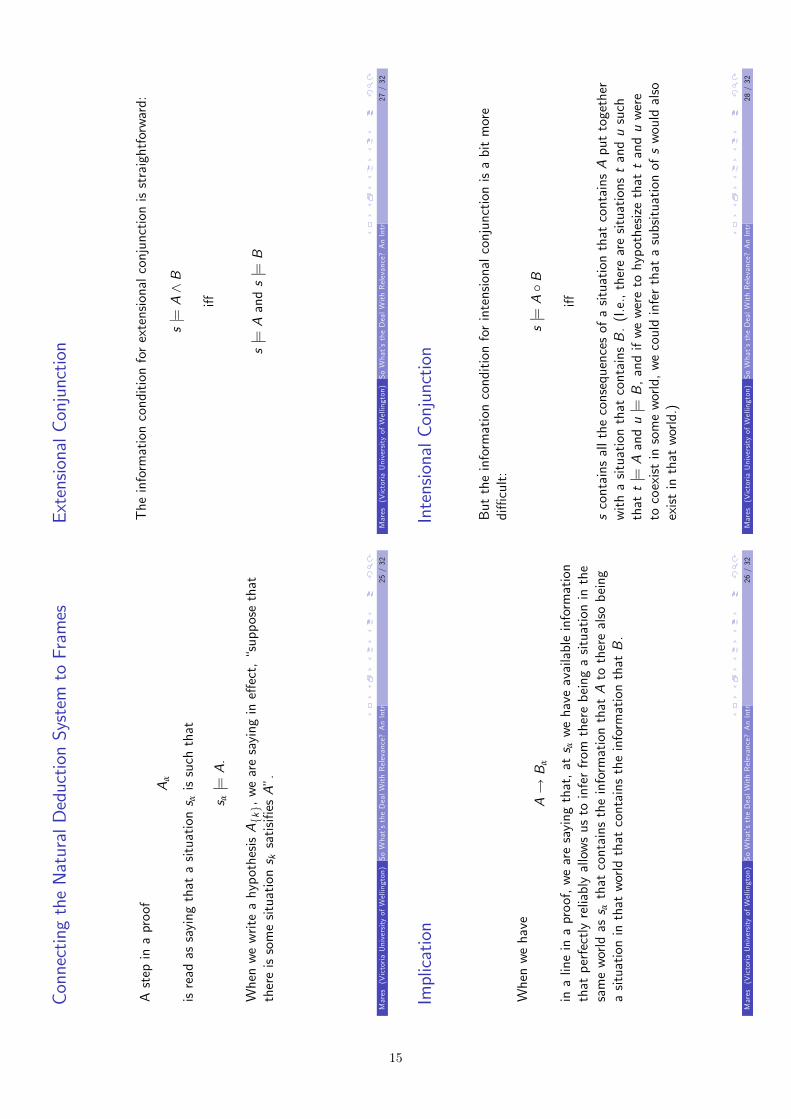
Theinformationconditionforextensionalconjunctionisstraightforward:

s|=A^B

i§

s|=Aands|=B

Mares

(VictoriaUniversityofWellington)SoWhat’stheDealWithRelevance?AnIntroductiontoRelevantLogic

27/32

IntensionalConjunction

Buttheinformationconditionforintensionalconjunctionisabitmore

di¢cult:

s|=AB

i§

scontainsalltheconsequencesofasituationthatcontainsAputtogether

withasituationthatcontainsB.(I.e.,therearesituationstandusuch

thatt|=Aandu|=B,andifweweretohypothesizethattanduwere

tocoexistinsomeworld,wecouldinferthatasubsituationofswouldalso

existinthatworld.)

Mares

(VictoriaUniversityofWellington)SoWhat’stheDealWithRelevance?AnIntroductiontoRelevantLogic

28/32

ConnectingtheNaturalDeductionSystem

toFrames

Astepinaproof

Aa

isreadassayingthatasituations aissuchthat

s a|=A.

WhenwewriteahypothesisA{k},wearesayingine§ect,“supposethat

thereissomesituations ksatisifiesA”.

Mares

(VictoriaUniversityofWellington)SoWhat’stheDealWithRelevance?AnIntroductiontoRelevantLogic

25/32

Implication

Whenwehave

A!B

a

inalineinaproof,wearesayingthat,ats awehaveavailableinformation

thatperfectlyreliablyallowsustoinferfrom

therebeingasituationinthe

sameworldass athatcontainstheinformationthatAtotherealsobeing

asituationinthatworldthatcontainstheinformationthatB.

Mares

(VictoriaUniversityofWellington)SoWhat’stheDealWithRelevance?AnIntroductiontoRelevantLogic

26/32

15

Thepresentsystem

validatescontraction:

X,A,A,Y

`C

X,A,Y

`C

andsomepeoplethinkthisisbad.(Butit’snot.)

Mares

(VictoriaUniversityofWellington)SoWhat’stheDealWithRelevance?AnIntroductiontoRelevantLogic

31/32

Butifwechangethenatureofthesubscripts,wealsohavetocomeup

withadi§erentinterpretationofthesystem.

Mares

(VictoriaUniversityofWellington)SoWhat’stheDealWithRelevance?AnIntroductiontoRelevantLogic

32/32

TheFalsum

s|=f

i§

sisanimpossiblesituation.

Mares

(VictoriaUniversityofWellington)SoWhat’stheDealWithRelevance?AnIntroductiontoRelevantLogic

29/32

Wecanmodifythenaturaldeductionsystem

inseveral

ways

Oneoftheeasiestisbychangingthenatureofthesubscripts:

Wecanmakethesubscriptsmultisetsratherthansets

Wecanmakethesubscriptssequences

Wemakethesubscriptsbinarytrees(structures,inthesenseof

Slaney-Restall)

Mares

(VictoriaUniversityofWellington)SoWhat’stheDealWithRelevance?AnIntroductiontoRelevantLogic

30/32

16

Paraconsistent Mathematics

Zach WeberUniversity of Otago

Overview

When we practice mathematics, we make some very intuitive assumptions that can triggercontradictions. Well known examples include the original infinitesimal calculus and naiveset theory, the latter based on naive comprehension:

9y8x(x 2 y $ A(x))

Paraconsistency is a method for preserving our original mathematical intuitions, by con-trolling for inconsistency with a weaker logical consequence relation, `.

‘Classical’ inferences

In a paraconsistent setting, classical inferences like ex falso quodlibet (A,¬A ` B) anddisjunctive syllogism (A,¬A _ B ` B) are not in general valid. Nevertheless, becauseparaconsistent theories are not trivial (i.e. some sentences are not satisfied), these infer-ences can be restored in appropriate forms. An absurdity constant is defined

? := 8x8yx 2 y

yielding the property that ? ` A for any sentence A. Then ex falso and disjunctivesyllogism are both valid when ¬A is replaced by the property that A entails ?. If wefurther identify

0 := {x : ?}, 1 := {0}then we find a consistency point at the bottom of the number line: 0 = 1 is absurd,and thus so is any sentence that implies 0 = 1. Using this consistency point, we canconfirm some structural facts that are very ‘far away’, such as N being unbounded inR, Konig’s Lemma (and Brouwer’s Fan Theorem), and the Heine-Borel Theorem. Acomplementary consistency point is generated at the top of the number line, at theuniversal set V = {x : 9yx 2 y}.

Connections with other areas

Paraconsistent mathematics thus o↵ers a way to control arguments in a more nuancedway (especially when the underling logic is a relevant logic). The logic makes ‘intensional’distinctions’, which is especially clear when we look at non-equivalent definitions of emptysets, such as {x : ?} and {x : x 6= x}. (The latter may have some members, even thoughit has no members.)

Paraconsistency is a natural dual to constructive mathematics, but it is not opposed toconstructivisim – in fact, constructive techniques are particularly powerful in paracon-sistent settings. The goals of the program are to recapture classical results, and extendthem into the study of the inconsistent, which is intrinsically interesting and beautiful inits own right, and which may yet find applications in any domain where inconsistency ispossible.

17

References

Getting started:

Inconsistent Mathematics, Internet Encyclopedia of Philosophy: http://www.iep.utm.edu/math-inc/

Recent papers:

Weber, Zach (2010). Transfinite Numbers in Paraconsistent Set Theory. Review of Symbolic Logic 3(1): 71-92.

McKubre-Jordens, Maarten and Weber, Zach (2012). Real Analysis in Paraconsistent Logic. Journal of Philo-sophical Logic, to appear.

See also:

Brady, Ross (2006). Universal Logic, CSLI. [****This book includes the classical model theoretic proofs that show

paraconsistent mathematics is not trivial.****]

Mortensen, Chris (1995). Inconsistent Mathematics. Kluwer Academic Publishers.

Priest, Graham (2006). In Contradiction: A Study of the Transconsistent. Oxford University Press. second

edition.

18

Constructive Methods in Mathematics

Maarten McKubre-JordensUniversity of Canterbury

In Brief

The point of using constructive methods in mathematics is to explicitly exhibit anyobject or algorithm that the mathematician claims exists; so constructive proof provides,in principle, a mechanical method. Loosely speaking, one replaces the absolute notion oftruth in mathematics, with (algorithmic) provability. Constructive proofs:

1. embody (in principle) an algorithm (for computing objects, converting other algo-rithms, etc.), and

2. prove that the algorithm they embody is correct (i.e. that it meets its design speci-fication).

Constructive techniques

Upon adopting only constructive methods, we lose some powerful proof tools in ourarsenal, such as unrestricted use of the Law of Excluded Middle (LEM) and anythingwhich validates it, such as double negation elimination and unrestricted use of proof bycontradiction1. We cannot, in general, constructively prove 9xP (x) by assuming ¬9xP (x)and deriving a contradiction; that doesn’t compute the required x.

However the news isn’t all bad. In a lot of cases, constructive alternatives to non-constructive classical principles in mathematics, leading to some very strong results. Forexample, the classical least upper bound principle is not constructively provable.

LUB Any nonempty set of reals that is bounded from above has a least upper bound.

However the constructive least upper bound principle is provable.

CLUB Any order-located nonempty set of reals that is bounded from above has a leastupper bound.

A set is order-located if given any real x, the distance from x to the set is computable. Itis quite common for a constructive alternative to be classically equivalent to the classicalprinciple; and, indeed, classically every nonempty set of reals is order-located.

To see why LUB is not provable, we may consider a so-called Brouwerian counterexample(or weak counterexample), such as the set

S = {x 2 R : (x = 2) _ (x = 3 ^ P )}

where P is some as-yet unproven statement, such as Goldbach’s conjecture. If the setS had a computable LUB, then we would have a quick proof of the Goldbach conjec-ture’s truth or of its unprovability. A Brouwerian counterexample is an example which

1Which is not to say that LEM is false. Both Russian recursive mathematics, in which LEM is provably false, and

classical mathematics, in which it is logically true, are models of constructive mathematics—so in a way, LEM is independentof constructive mathematics, and hence non-constructive.

19

shows that if a certain property holds, then it is possible to constructively prove a non-constructive principle (such as LEM); and thus the property itself must be essentiallynon-constructive.

It is often the case that a classical theorem becomes more enlightening when seen fromthe constructive viewpoint2. For example, in the least upper bound principle the extracomputational information provided by being order-located is enough to guarantee thecomputability of the least upper bound.

Within constructive mathematics a number of methods has been developed, enrichingthe subject to a degree where it is comparable to its classical counterpart in complexity,and often exceeds it in computational informativity.

Connections with other disciplines

The connection of constructive mathematics with computer science and programming isclear. A major upshot of the constructive approach is to identify with relative ease thesorts of things that computers cannot do (it is usually easier to prove a negative result),and so to guide the programmer to focus on what is achievable.

Like paraconsistency, constructivism brings out finer-grained details of proof that areoften casually dismissed in classical proofs. In fact, a single classical theorem can lead toseveral constructively discernible di↵erent theorems, where the constructive techniquesbring to the fore extra computational strength required in the hypotheses, or furtherinformation contained in the conclusion.

References

For a more in-depth introduction:

Bridges, D.S. Constructive Mathematics. Stanford Encyclopedia of Philosophy: http://plato.stanford.edu/

entries/mathematics-constructive/

Further reading:

Aberth, O. (1980) Computable Analysis. New York: McGraw-Hill.

Aczel, P., and Rathjen, M. (2001) Notes on Constructive Set Theory. Report No. 40, Institut Mittag-Le✏er,Royal Swedish Academy of Sciences.

Beeson, M.J. (1985) Foundations of Constructive Mathematics. Heidelberg: Springer-Verlag.

Bishop, E. and Bridges, D.S. (1985) Constructive Analysis. Grundlehren der math. Wissenschaften, Heidelberg:Springer-Verlag.

Bridges, D.S. and Richman, F. (1987) Varieties of Constructive Mathematics. Cambridge: Cambridge UniversityPress.

Bridges, D.S. and Vıta, L.S. (2006) Techniques of Constructive Analysis. Universitext, Heidelberg: Springer-Verlag.

Dummett, M. (2000) Elements of Intuitionism. Oxford Logic Guides 39, Oxford: Clarendon Press.

Martin-Lof, P. (1968) Notes on Constructive Analysis. Stockholm: Almquist & Wixsell.

Weirauch, K. (2000) Computable Analysis. EATCS Texts in Theoretical Computer Science, Heidelberg: Springer-

Verlag.

2Although it would be unfair to say that constructive mathematics is revisionist in nature. Indeed, Brouwer proved his

fan theorem intuitionistically in 1927, but the first proof of Konig’s lemma (its classical equivalent) was published in 1933.

20

Dothefollowingstatem

ents

Ithefour

colour

theorem,

IFermat’sgreattheorem,

ItheRiemannhypothesis,

ItheCollatz

conjecture

shareacommon

mathematical

prop

erty?

And

,ifthereissuch

aprop

erty,how

canweuseitforabetter

understand

ingof

thesestatem

ents?

3/19

9

Com

putabilityandCom

plexity

1

Universalitytheo

rem.There

exists

(and

canbeconstructed)

a(Turing)

machine

U—calleduniversal—such

that

foreverymachine

Vthereexists

aconstant

c=

c

U,V

such

that

foreveryprogram

�thereexists

a�0forwhich

thefollowingtwocond

itions

hold:

IU(�

0 )=

V(�),

I|�

0 |

|�|+

c.

4/19

9

Aconstructiveapproachtothe

complexityofmathematical

problems

C.S.Calud

e(U

oA)andE.Calud

e(M

asseyU)

Con

struMathSou

th2012,Wesport

1/19

9

Thistalk

presents

onoverview

ofresultsob

tained

withan

algorithmic

uniform

metho

dto

measure

thecomplexityof

alarge

classof

mathematical

prob

lemsanddiscussesafew

open

prob

lems.

2/19

9

21

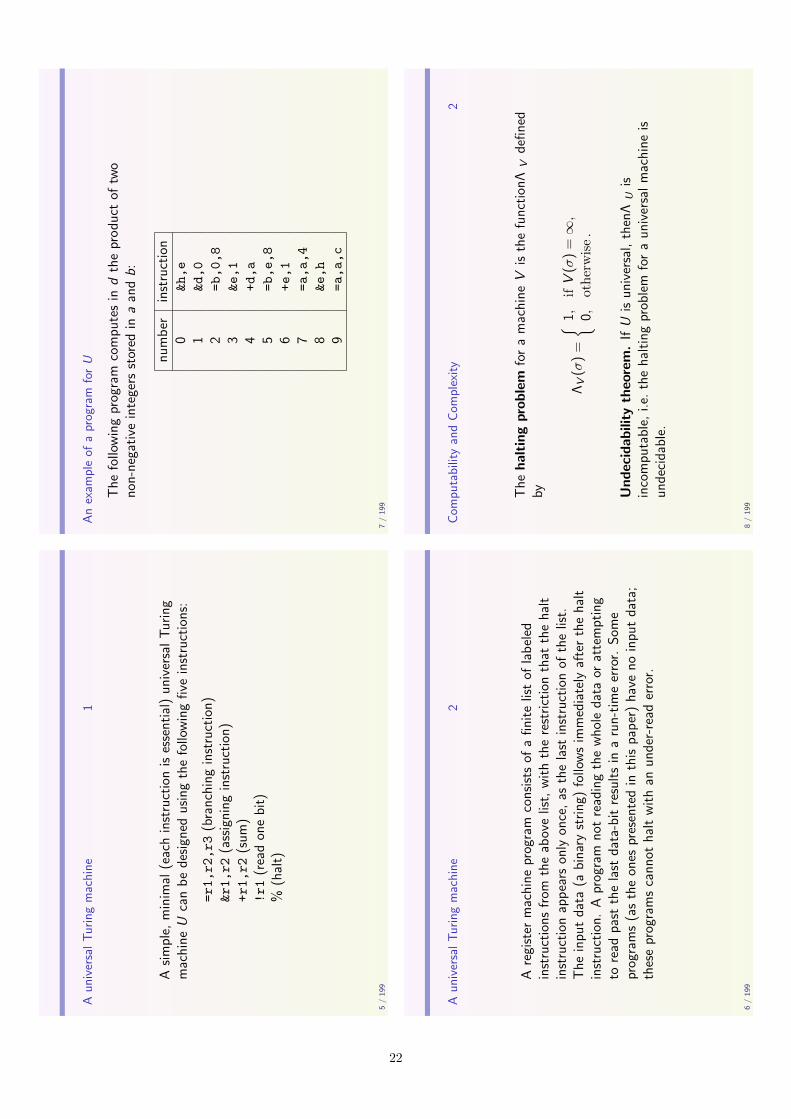
Anexam

pleof

aprog

ram

forU

The

followingprogram

compu

tesin

dtheprod

uctof

two

non-negative

integers

stored

inaandb:

number

instruction

0&h,e

1&d,0

2=b,0,8

3&e,1

4+d,a

5=b,e,8

6+e,1

7=a,a,4

8&e,h

9=a,a,c

7/19

9

Com

putabilityandCom

plexity

2

The

haltingproblem

foramachine

Visthefunction

⇤V

defin

edby

⇤V(�)=

⇢1,

ifV(�)=

1,

0,otherwise.

Undecidab

ility

theo

rem.IfU

isun

iversal,then⇤

Uis

incompu

table,

i.e.thehaltingprob

lem

foraun

iversalmachine

isun

decidable.

8/19

9

Aun

iversalTuringmachine

1

Asimple,

minim

al(eachinstructionisessential)un

iversalTuring

machine

Ucanbedesign

edusingthefollowingfiveinstructions:

=r1,r2,r3(branching

instruction)

&r1,r2(assigning

instruction)

+r1,r2(sum

)!r1(readon

ebit)

%(halt)

5/19

9

Aun

iversalTuringmachine

2

Aregister

machine

program

consists

ofafin

itelistof

labeled

instructions

from

theab

ovelist,withtherestrictionthat

thehalt

instructionappears

only

once,as

thelast

instructionof

thelist.

The

inpu

tdata

(abinary

string

)followsim

mediately

afterthehalt

instruction.

Aprogram

notreadingthewho

ledata

orattempting

toread

past

thelast

data-bitresultsin

arun-timeerror.

Som

eprograms(astheon

espresentedin

thispaper)have

noinpu

tdata;

theseprogramscann

othaltwithan

under-read

error.

6/19

9

22

Com

plexity

Complexity

C

U(⇡)=

min{|⇧P|:⇡=

8nP(n)}.

Invarian

cetheo

rem.IfU,U

0areun

iversal,then

thereexists

aconstant

c=

c

U,U

0such

that

forall⇡=

8nP(n),P

compu

table:

|CU(⇡)�C

U0 (⇡)|

c.

Inco

mputability

theo

rem.IfU

isun

iversal,then

C

Uis

incompu

table.

11/19

9

Com

puting

thesize

oftheprog

ram

MULT

number

instruction

code

leng

th0

&h,e

010001001

00110

141

&d,0

0100101

100

102

=b,0,8

00011

100

1110010

153

&e,1

0100110

101

104

+d,a

111

00101

010

115

=b,e,8

00011

00110

1110010

176

+e,1

111

00110

101

117

=a,a,4

00010

010

11010

138

&e,h

0100110

0001001

149

=a,a,c

00010

010

00100

13

Total

leng

th:128.

12/19

9

⇧1–problem

s

Aprob

lem

⇡of

theform

8�P(�),

where

Pisacompu

tablepredicateiscalleda⇧

1–problem.

IAny⇧

1–problem

isfin

itelyrefutable.

IFor

every⇧

1–problem

⇡=

8�P(�)weassociatetheprogram

⇧P=

inf{n:P(n)=

false}

which

satisfies:

⇡istrue

i↵U(⇧

P)=

1.

ISolving

thehaltingprob

lem

forU

solves

all⇧

1–problem

s.

9/19

9

Examples

The

prob

lems

Ithefour

colour

theorem,

IFermat’sgreattheorem,

ItheRiemannhypothesis,

ItheCollatz’sconjecture

areall⇧

1–problem

s.

Ofcourse,no

tallprob

lemsare⇧

1–problem

s.For

exam

ple,

the

twin

prim

econjecture.

10/19

9

23

Riemannhypothesispredicate

The

negation

oftheRiemannhypothesisisequivalent

tothe

existenceof

positiveintegers

k,l,m

,nsatisfying

thefollowing:

1.n�

600,

2.8y

<n[(y+1)

|m],

3.m

>0&8y

<m[y

=0_9x

<n[¬

[(x+1)

|y]]],

4.explog(m

�1,l),

5.explog(n

�1,k),

6.(l�n)2

>4n

2k

4,

where

x|z

means

“xdividesz”andexplog(a,b)isthepredicate

9x[x

>b+1&(1

+1/

x)x

b

a+1<

4(1+1/x)x

b].

15/19

9

The

Collatz

conjecture

Given

apositiveintegera

1thereexists

anaturalN

such

that

a

N=

1,where

a

n+1=

⇢a

n/2,

ifa

niseven,

3an+1,

otherwise.

The

Collatz

conjecture

isa⇧

1-statement,bu

ttheproo

fis

non-constructive!Writing

The

Collatz

conjecture

asa

⇧2-statement(i.e.of

theform

8n9i

R(n,i),where

R(n,i)isa

compu

tablepredicate)

iseasy

andconstructive.

How

togeneralisethecomplexitymetho

dfor⇧

2-statements?

16/19

9

Com

plexityClasses

Because

oftheincompu

tabilitytheorem,weworkwithup

per

bou

ndsforC

U.Astheexactvalueof

C

Uisno

tim

portant,we

classify⇧

1–problem

sinto

thefollowingclasses:

CU,n=

{⇡:⇡isa⇧

1–problem

,CU(⇡)

nkb

it}.

13/19

9

Som

eResults

ICU,1:Legendre’sconjecture(there

isaprim

enu

mber

between

n

2and(n

+1)

2,foreverypositiveintegern),Fermat’slast

theorem

(there

areno

positiveintegers

x,y

,zsatisfying

the

equation

x

n+y

n=

z

n,foranyintegervaluen>

2)and

Goldbach’sconjecture(every

even

integergreaterthan

2can

beexpressedas

thesum

oftwoprim

es)

ICU,2:Dyson’sconjecture(the

reverseof

apow

erof

twois

neverapow

erof

five)

ICU,3:theRiemannhypothesis(allno

n-trivialzerosof

the

Riemannzeta

function

have

real

part

1/2),Euler’sinteger

partitiontheorem

(the

number

ofpartitions

ofan

integerinto

oddintegers

isequalto

thenu

mber

ofpartitions

into

distinct

integers).

ICU,4thefourcolourtheorem

(the

vertices

ofeveryplanar

graphcanbecoloured

withat

mostfour

coloursso

that

notwoadjacent

vertices

receivethesamecolour)

14/19

9

24

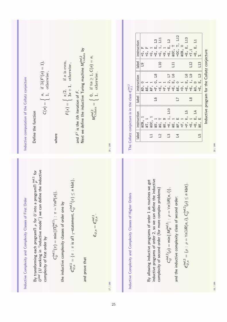
Indu

ctivecompu

tation

oftheCollatz

conjecture

Define

thefunction C(n)=

⇢n,

if9i(F

i (n)=

1),

1,otherwise,

where

F(x)=

⇢x/2,

ifxiseven,

3x+1,

otherwise,

andF

iistheith

iterationof

F.

Nextwedefin

etheindu

ctiveTuringmachine

M

ind,2

Collatz

by

M

ind,2

Collatz

=

⇢0,

if8n

�1,C(n)=

n,

1,otherwise.

19/19

9

The

Collatz

conjecture

isin

theclassCind,2

U,1

label

instruction

label

instruction

label

instruction

&OR,1

&D,0

L9

+G,F

&T,1

&E,1

+G,F

L1

&OC,1

&F,1

+G,1

&N,1

L6

=F,G,L8

=E,E,L3

L2

&G,T

+E,1

L10

=G,1,L11

&K,N

+F,1

+N,1

L3

=K,1,L10

=E,2,L7

=E,E,L2

&E,1

=E,E,L6

L11

&OC,T

L4

&F,E

L7

&E,0

=OC,T,L12

+F,1

+D,1

&OR,0

=F,K,L5

=E,E,L6

=E,E,L13

+E,1

L8

=E,1,L9

L12

+T,1

=E,E,L4

&G,D

=E,E,L1

L5

&K,E

=E,E,L3

L13

%

Indu

ctiveprogram

fortheCollatz

conjecture

20/19

9

Indu

ctiveCom

plexityandCom

plexityClasses

ofFirst

Order

Bytransformingeach

program⇧

PforU

into

aprogram⇧

ind,1

Pfor

U

ind(U

working

in“ind

uctive

mod

e”)wecandefin

etheindu

ctive

complexityof

first

orderby

C

ind,1

U(⇡)=

min{|⇧ind,1

P|:⇡=

8nP(n)},

theindu

ctivecomplexityclassesof

orderon

eby

Cind,1

U,n

={⇡

:⇡isa⇧

1–statement,C

ind,1

U(⇡)

nkb

it},

andprovethat

CU,n=

Cind,1

U,n

.

17/19

9

Indu

ctiveCom

plexityandCom

plexityClasses

ofHigherOrders

Byallowingindu

ctiveprogramsof

order1as

routines

weget

indu

ctiveprogramsof

order2,

sowecandefin

etheindu

ctive

complexityof

second

order(for

morecomplex

prob

lems)

C

ind,2

U(⇢)=

min{|M

ind,2

R|:⇢=

8n9iR(n,i)},

andtheindu

ctivecomplexityclassof

second

order:

Cind,2

U,n

={⇢

:⇢=

8n9iR(n,i),C

ind,2

U(⇢)

nkb

it}.

18/19

9

25

References2

C.S.Calud

e,E.Calud

e,K.Svozil.The

complexityof

provingchaoticity

andtheChu

rch-TuringThesis,Chaos20

0371

03(201

0),1–

5.

C.S.Calud

e,M.J.

Dinneen.Exact

approxim

ations

ofom

eganu

mbers,

Int.JournalofBifurcation&

Chaos17

,6(200

7),19

37–1

954.

E.Calud

e.The

complexityof

Riemann’sHyp

othesis,Journalfor

Multiple-ValuedLogicandSoftComputing,(201

2),to

appear.

E.Calud

e.Fermat’sLastTheorem

andchaoticity,NaturalComputing,

(201

1),DOI:10

.100

7/s110

47-011

-928

2-9.

M.J.

Dinneen.A

prog

ram-sizecomplexitymeasure

formathematical

prob

lemsandconjectures,in

M.J.

Dinneen,B.Kho

ussainov,A.Nies

(eds.).Computation,PhysicsandBeyond,Springer,Heidelberg,

2012

.

J.Hertel.OntheDi�

cultyof

Goldb

achandDyson

Con

jectures,

CDMTCSResearchReport36

7,20

09,15

pp.

23/19

9

References3

J.Lagarias(ed.),TheUltimateChallenge:The3x

+1Problem,AMS,

2010

.

C.Moo

re,S.Mertens.TheNatureofComputation,OxfordUniversity

Press,Oxford,

2011

.

G.Perelman.Ricci

Flow

andGeometrization

ofThree-M

anifolds,

Massachusetts

Instituteof

Techn

olog

y,Departm

entof

Mathematics

Sim

onsLecture

Series,September

23,20

04.

24/19

9

Twoop

enprob

lems

Whatisthecomplexityof

IPvs

NPprob

lem?

IPoincare’stheorem

(Perelman)?

21/19

9

References1

M.Burgin,

C.S.Calud

e,E.Calud

e.Indu

ctivecomplexitymeasuresfor

mathematical

prob

lems,in

preparation.

C.S.Calud

e,E.Calud

e,M.J.

Dinneen.A

new

measure

ofthedi�culty

ofprob

lems,JournalforMultiple-ValuedLogicandSoftComputing12

(200

6),28

5–30

7.

C.S.Calud

e,E.Calud

e.Evaluatingthecomplexityof

mathematical

prob

lems.

Part1ComplexSystems,18

-3(200

9),26

7–28

5.

C.S.Calud

e,E.Calud

e.Evaluatingthecomplexityof

mathematical

prob

lems.

Part2ComplexSystems,18

-4,(201

0),38

7–40

1.

C.S.Calud

e,E.Calud

e.The

complexityof

theFou

rColou

rTheorem

,LMSJ.Comput.Math.13

(201

0),41

4–42

5.

C.S.Calud

e,E.Calud

e,M.Queen.The

complexityof

theinteger

partitiontheorem,TheoreticalComputerScience,accepted.

22/19

9

26

Abstract Stone Duality - A Logic for Topology

Nicholas DuncanUniversity of Canterbury

Abstract

Abstract Stone Duality (ASD) is a logical system for reasoning and computing with topologicalspaces. Compared to other systems of logic the quantifiers 8 and 9 are restricted to compact and overtspaces, respectively, in ASD. The concept of overt spaces is not seen in topology, as all topologicalspaces are overt, but they play an important computational role in ASD.

In this paper we start with the definition of topology and relate it to computability. Then wefocus on the construction of the type theory underlying ASD, starting with the types, which representspaces, moving on to terms, which represent continuous functions, and finally reaching judgements,which deal with proving results in the calculus.

Next we will consider how local compactness allows computation in the calculus and the con-nection to interval arithmetic. Finally we compare this system to other computable systems, likeRecursive Analysis.

Introduction

Abstract Stone Duality (ASD) is a logical system created by Paul Taylor for reasoningand computing with topological spaces. It is named after Stone’s duality between Booleanalgebras and Stone spaces. This duality manifests itself in the fact that spaces are alsoalgebras, so we can avoid the use of sets by using the spaces as carriers of those algebras.However, in this article we will not dwell on this important aspect of ASD, instead wewill focus on the logic. This system is given as an example of a logic that is suitable fora specific domain in mathematics.

Instead of starting with a large all-encompassing system, such as a set theory, and thenplacing continuous and computable structures on sets, we begin with a logical system inwhich everything is computable and continuous and the operations of the system preservethese properties.

This system is a type theory whose types represent topological spaces, and the terms ofthe calculus represent continuous functions. Everything that can be constructed preservescontinuity and computability.

A major restriction in this system is that quantifiers may only range over certain kindsof spaces. The universal quantifier 8 can only quantify over compact spaces, like theunit interval [0, 1], but not N or Q. The existential quantifier 9 can only quantify overovert spaces. Classically all topological spaces are overt, however in some constructivetopological settings like locale theory not all spaces are overt. Many of the spaces in ASDare overt, like N, Q, and R, however not all spaces are overt. Indeed those that are overtembody some computational process to access their elements. The subspace of all zerosof a function is often not overt, since deciding whether a real number is equal to zero isnot computable.

Parts of this calculus, like the real numbers, can be transformed into programs usinginterval arithmetic. The calculus insures that these programs succeed and return aninterval solution to within a given tolerance. This way results can be extracted from thecalculus.

27

In comparison with other approaches to computable topology the closed interval [0, 1]is compact in ASD. This allows us to use the universal quantifier over closed boundedintervals, which is vital for the translation to interval arithmetic.

Topology and Observability

We start with the definition of a topological space.

Definition 1. A topological space consists of a set X of points along with a set T ofsubsets of X, whose elements are called open subsets, such that

• The subsets ; and X are open subsets.

• If U and V are open subsets so is U \ V .

• If {Ui}i2I is a collection of open subsets thenS

i2I Ui is an open subset.

Example 2. The real numbers R has the Euclidean topology where the open sets arearbitrary unions of open intervals (a, b):

U =[

i

(ai, bi), where (ai, bi) = {x 2 R | ai < x < bi}

We compare the definition of open subsets with the concept of observable properties ofa set. An observable property is some subset in which membership is semi-decidable. Anon-rigorous definition is the following:

Definition 3. Let X be a set. A subset S of X is observable if there is a computerprogram, such as a Turing machine, which when given an encoding of an element x of X,halts if x 2 S, or loops (runs forever) otherwise.

Example 4. The standard example of observable subsets are the recursively enumerablesubsets of N. Every recursively enumerable subset is given by a computer program, andan element x is in a recursively enumerable subset if and only if this computer programhalts on input x.

There are some similarities between open subsets of a topological space and observablesubsets:

• The subset ; is observable, just use a program which runs forever. This programnever halts, so it does not accept any element of X.

• The subset X is observable, use the program which immediately halts.

• If U and V are observable with programs u and v, then U \ V is observable. Takethe program which runs u until it halts, then it runs v. If x is in U and V thenboth programs halt, so x is in U \ V . If x is not in both U and V then one of theprograms will loop on input x. This shows that U \ V is observable.

• Let (Ui)i2N be a sequence of observable subsets, where the sequence of acceptingprograms is also computable (e.g. if the computer programs are encoded by numbersui, then the function i 7! ui should be computable). Then U =

Si2N Ui is also

observable.

28

To see this let (ui) be the sequence of computer programs in which ui accepts Ui.We construct a computer program u that takes an input x and interleaves the com-putations of each ui(x), terminating as soon as one ui(x) terminates. This programcould perform one step of u

0

(x), then one step of u0

(x) and u1

(x), then another ofu0

(x), u1

(x) and u2

(x), and so on. Each loop we introduce a new program in the se-quence. Since the sequence is computable this method of introducing new programsis also computable.

If x is in some Ui then eventually the program ui will halt. If x is not in any of thesubsets Ui then each program ui will loop on input x, so the program u above willalso loop on x. Hence the union is observable.

So we see that observable properties have binary intersections, but only some unions,and the indexing set of these unions must somehow be computable. If the sequence (Ui)was not computable then we cannot construct a new program in each iteration of theprogram u above. Furthermore, if the indexing set of the union is not countable then wecannot interleave the operations like we did in u, and we would miss some elements ofthe indexing set.

In ASD we do not have all unions, but we do have computable unions like in the observablesubsets case. The indexing spaces of these unions will be overt spaces, which we will defineshortly. If a collection of open subspaces is indexed by an overt space then the union isopen. However not all spaces are overt, so we do not have all unions.

Open Subsets vs Predicates vs Functions

Instead of treating observable properties as subsets we will treat them as continuousfunctions of a special kind. This will reduce the number of primitive concepts that wehave to consider. First we give the definition of a continuous function.

Definition 5. Given spaces X and Y a continuous function f : X ! Y is a functionsuch that for every open subset U of Y the inverse image f�1(U) is an open subset ofX. The inverse image of U is the set:

f�1(U) = {x 2 X | f(x) 2 U}

To treat open subsets as continuous functions we need a special topological space, calledthe Sierpinski space.

Definition 6. The Sierpinski space ⌃ classically consists of two points, which we call Tand F , and the topology consists of the three subsets ;, ⌃ and {T}. Note that {F} isnot open.

Given a continuous function � : X ! ⌃ we have an open subset ��1({T}) of X. Con-versely, given any open subset U of X we can define a continuous function X ! ⌃, whichclassically is defined by f(x) = T if x 2 U , or f(x) = F otherwise.

This construction gives us a correspondence between continuous functions X ! ⌃ andopen subsets of X. This can be further extended to closed subsets of X, which classicallyare the set complements of open subsets. A closed subset is given by the inverse imageof the closed set {F}.Now let us consider the continuous functions⌃ ! ⌃. We know that these correspond toopen subsets of⌃ , of which classically there are three: ;, ⌃ and {T}. They correspond

29

to the continuous functions F (constantly false), T (constantly true), and the identityfunction.

Notice that there is no continuous function which swaps T and F . This has importantcomputational significance. The space ⌃ can be thought of as the space of terminationpossibilities of a computer program - either a program terminates (T ), or a program loops(F ). If we think of a space X as the space of inputs of a program, and f : X ! ⌃ asa computer program recognising an observable property, then f(x) = T if the programhalts, or f(x) = F if the program loops.

If we had a function ¬ : ⌃ ! ⌃ which swaps T and F then the set complement ofany observable property would also be observable, just take the corresponding functionf : X ! ⌃ and post-compose with ¬. In the recursively enumerable subset examplethis would mean that co-recursively enumerable subsets would also be observable, sothe halting problem would be decidable. This is not computable, so we would losecomputational ability if ¬ was an acceptable function. Luckily the topology of ⌃ preventsthis behaviour.

Objects of ASD

We have seen that open subsets of a space X can be represented by a continuous functionX ! ⌃. The calculus allows us to abstract away from the set theoretic nature of topolo-gies, and so instead of considering open subsets of a space X we will consider continuousfunctions X ! ⌃. Since we also want to abstract away from the set-theoretic nature offunctions we use the word morphism instead of continuous function.

ASD is a type theory whose types represent spaces. How do we represent the topology ona space X? Classically it is given by a collection of subsets of X, but we have seen thatthese subsets may be represented by morphisms X ! ⌃. To avoid the use of sets thiscollection of morphisms, which we denote⌃ X , should itself be a space. So the topologyof a space X in ASD is itself a space,⌃ X . Classically, for this to be a suitable space Xmust be a locally compact topological space, and then we can give⌃ X the Scott topology.Locally compact spaces will be considered later on in this article, but we will not coverthe Scott topology. See [6] for details. So the classical model of ASD will interpret thetypes as locally compact topological spaces.

Suppose we have interpretations for the types X and⌃ X , how do we ensure that ⌃X is thetopology on X? For this we use a notion from category theory called a monad. If you donot know about monads then feel free to skip this paragraph. Monads allow us to definealgebras whose carriers are not necessarily sets, and the arity of the operations in thealgebra do not need to be indexed by sets. We require that the adjunction (⌃(�) a ⌃(�))be monadic, where⌃ (�) is the exponential functor. This makes the objects ⌃-algebras,and this method bypasses any requirements of underlying sets. For more details see [5].

This leads us to our first axiom, which gives the types of ASD. The calculus of ASDconsists of four syntactic elements: types, terms, statements, and judgements. Many ofthese depend on each other, so the formal definition of the calculus requires a mutuallyinductive definition. We will give parts of the calculus independently, and some stagesmay refer to future stages of definition. This is not intrinsic to ASD itself, as other typetheories have this di�culty.

Axiom 1. The types of ASD consist of the following:

• The basic types 1, ⌃ and N.

30

• If X is a type then so is⌃ X .

• If X and Y are types, so is X ⇥ Y .

• Technical condition: If X is a type then any ⌃-split subspace is also a type. Thisconstruction comes from the monad above, and allows the construction of a varietyof derived types. These types are denoted by {X |E}, where E is a special term oftype⌃ X⇥⌃

Xcalled a nucleus. See [4] for details on this construction.

The derived types of ASD can be constructed from the type constructors above, and theyinclude the empty space 0, Q, R, [0, 1], and many other spaces.

In a model of ASD these types are sent to certain objects, but note that the derived typeR need not necessarily be interpreted as the real numbers. In certain constructive settingsthe closed interval [0, 1] is not compact, so R can not be interpreted as the standard realnumbers in such a setting. Also note that the classical interpretation of Q is with thediscrete topology, not the order topology. We will see more of this later.

Logical Terms of the Calculus

Now we will consider the logical terms of the calculus, which will represent logical prop-erties and subspaces. The terms of type ⌃ are called propositions, and the terms of type⌃X are called predicates.

Axiom 2. The logical terms of ASD consist of the following:

• Variables: The types ⌃ and⌃ X all have a countable supply of variables, oftendenoted �,⌧ for propositions and �, for predicates. Each variable has an associatedtype.

• Constants: >,? are terms of type⌃ , which represent true and false.

• Connectives: if � and ⌧ are terms of type⌃ , the connectives � _ ⌧ and � ^ ⌧ areterms of type ⌃, representing disjunction and conjunction, respectively.

• �-abstraction: if �(x) is a term of type ⌃ with a free variable x of type X then�x.�(x) is a term of type ⌃X . �-abstraction is used to construct functions in typetheory.

• �-application: if � is a term of type⌃ X and a is a term of type X, then �(a) is aterm of type ⌃. This term is also denoted �a.

• Equality: if N is a discrete space and n and m are terms of type N , then n =N mis a term of type ⌃.

• Inequality: if H is a Hausdor↵ space and n and m are terms of type H, then n 6=H mis a term of type ⌃.

• Universal quantification: If X is compact and �(x) is a term of type ⌃ with a freevariable x of type X, then 8x : X.�x is a term of type ⌃.

• Existential quantification: Similarly, if X is overt, then 9x : X.�x is a term of type⌃.

31

Note that we do not have the connectives ¬ or ! of type⌃ . These would lead tonon-computability, as we have seen earlier.

These logical terms require us to consider certain kinds of spaces. The discrete, Hausdor↵and compact spaces have their regular interpretation in topology. However, classicallyall spaces are overt, so the concept does not show up in classical topology.

First we consider the discrete spaces. These are spaces in which equality is observable.Classically this corresponds to spaces whose diagonal subset

{(x, x) 2 X ⇥X | x 2 X}

is open, which implies that all subsets are open. In ASD the spaces N,Z and Q arediscrete. Note that R is not discrete. If we consider real numbers as infinite decimalexpansions then to check equality we are required to check the entire expansion, which isnot observable as it would take an infinite amount of time.

Next are the Hausdor↵ spaces. In these spaces inequality is observable. Classicallythese correspond to Hausdor↵ topological spaces, where the diagonal is closed. In ASDthe spaces N,Z,Q,R, and [0, 1] are all Hausdor↵. Classically all discrete spaces areHausdor↵, but this is not so in ASD. Open subsets are not closed under arbitrary unions,so the classical proof that discrete implies Hausdor↵ does not apply.

The compact spaces correspond to the compact spaces in topology, which classically aregiven by the finite subcover property:

Definition 7. A topological space X is compact if for any family of open subsets {Ui}i2Iwhose union is the whole space X, there is a finite subset J of I such that the subfamily{Uj}j2J also covers the whole space X.

Note that we do not require compact spaces to be Hausdor↵. In ASD the bounded closedintervals [a, b] are compact, as well as the Sierpinski space ⌃ .

The overt spaces are invisible in classical topology. A topological space X is overt if theunique continuous function X ! 1 sends open subsets to open subsets. Classically alltopological spaces are overt, however in constructive locale theory not all spaces havethis property. Earlier terminology from locale theory called overt spaces open spaces,as the unique map X ! 1 is open. However this clashes with the terminology for opensubspaces, so overt spaces are the preferred terminology.

In locale theory an overt locale has a positivity predicate Pos(a), which holds if a isinhabited. Constructively not all non-empty subsets are inhabited, i.e. have an element,so overt spaces have a way of recognizing when an open is inhabited.

32

Here is a chart taken from [1], Examples 4.26, which gives a variety of di↵erent types ofASD and the properties they have:

space overt discrete compact Hausdor↵

N⇥ ⌃ X 7 7 7

R,Rn X 7 7 X⌃ X 7 X 7

[a, b], 2N X 7 X Xfree SK-algebra X X 7 7

N,Z,Q X X 7 XK-finite X X X 7

finite X X X Xset of codes ofnon-terminatingprograms

7 X 7 X

The free SK-algebra is the free algebra with a non-associative operation x ·y and symbolsS and K such that the two equalities:

((S · x) · y) · z = (x · z) · (y · z) and (K · x) · y = x

hold. This represents combinatory logic with the combinators S and K. Equality isobservable, as we can loop through all possible equalities. However, inequality is notobservable, as programs can be represented as combinators.

K-finite spaces correspond to spaces in which all the elements can be finitely listed, butthere may be repetitions, as inequality is not observable. Some examples are subspacesof a finite space given by a semi-decidable predicate.

Other Terms of the Calculus

Now that we have considered the logical terms we move on to the other terms of thecalculus.

Axiom 3. Non-logical terms of ASD.

Variables: Every term has a countable supply of variables. Each variable has a distin-guished type.

Product terms:

• If s is a term of type S, and t is a term of type T , then hs, ti is a term of type S⇥T ,representing an ordered pair.

• If x is a term of type S ⇥ T , then ⇡1

x is a term of type S and ⇡2

x is a term of typeT . These represent projections from an ordered pair to one of its components.

Numerical terms:

• Zero: 0 is a term of type N.

33

• Successor: If n is a term of type N, then Sn is a term of type N.

• Definition by description: If �(n) is a term of type ⌃ with a free variable n of typeN then the n.�n is a term of type N if the two statements:

�n ^ �m ) n =N m and 9n : N.�n , >

hold. Since we have not covered statements yet these can be read as the uniquenessand existence properties of definition by description.

• We also have terms for primitive recursion over any type.

Note that definition by description turns logical predicates into terms of type N. Thisallows unbounded minimization to be represented in the calculus, so we can representall partial recursive functions. However unbounded minimization implies that equality inthe calculus is no longer decidable, but we wanted to represent all computable functions,so this is not a problem.

We can derive more predicate terms from the ones above, like ,�, <,> for N and Q,by using primitive recursion and equality.

There are also derived terms for the derived types. For example the real numbers havethe following derived terms, which we give as an axiom:

Axiom 4. The type R has the following terms:

• Constants: 0 and 1 are terms of type R. Note that 0 is di↵erent from the term 0 oftype N, so we use context to determine which term we mean.

• Operators: If x and y are terms of type R, then x+ y, x⇥ y, x� y are terms of typeR. If we have the judgement y > 0 _ y < 0 , >, then x÷ y is a term of type R.

• Dedekind cuts: Given predicates � and ⌫ of type⌃ Q, or even of type ⌃R, thencut du.�d ^ ⌫u is a term of type R if the following six judgements hold:

9e.(d < e) ^ �e , �d 9t.⌫t ^ (t < u) , ⌫u

9d.�d , > 9e.⌫e , >�d ^ ⌫u ) d < u � d_ ⌫u ( (d < u)

These judgements have been organised into two columns to illuminate the symmetrybetween them. The first line states that the cuts are rounded, so have no maximumor minimum elements. The next line states that the cuts are inhabited. The fifthjudgement states that cuts are disjoint, and the final judgement states that cuts areorder-located.

This axiom is not strictly necessary, as the reals can be constructed in the calculus, butit is useful to see the properties of the real numbers. See [1] for the construction of Rfrom the basic types.

Statements and Judgements

We have given many of the terms of the calculus, the next thing to consider are thestatements. These describe a relationship, such as equality, between two terms.

Definition 8. There are two types of statements :

34

• If a and b are terms of type X, then a = b is a statement. Note we have no subscripton the equality sign. Such a statement expresses the fact that a and b represent thesame element of X.

• If ↵ and � are terms of type⌃ X , then ↵ ) �, ↵ ( � and ↵ , � are statements.The statement ) states that the open subspace corresponding to ↵ is included inthe open subspace corresponding to �. The statement , is the same as =, but wewill use the form , for predicates.

We stated earlier that ¬ and ! are not terms of type⌃ , so are not propositional connec-tives. However we can use statements to give some form of negation or implication. Theproposition a ! b can be represented as a ) b, and ¬a can be represented by a ) ?.However the logic is limited, in which we can only have one implication or negation, andit must occur as the outermost connective.

Finally we reach judgements, which are used to express some logical truth in our system.

Definition 9. A context � for a judgement consists of two lists. One list of variabledeclarations, e.g n : N, and another list of statements, where the free variables of thestatements occur in the first list.

Example 10. The following is a valid context:

n : N,� : ⌃N,�n, >

Definition 11. There are three types of judgements:

• Valid type formation: This has the form ` X : type, and states that X is a validtype.

• Term formation: This has the form� ` a : X, which states that a is a valid term oftype X in the context�.

• Statement formation: Similarly this has the form� ` s : X, where s is a statementbetween terms of type X. This states that the statement s holds in the context�.

Note that type formation does not have a context, so we cannot form types which dependon terms, or dependent types as they are called in type theory. Future extensions of thecalculus may allow such types.

We have given a large part of the syntax of the calculus, so now we will consider how tointerpret this syntax. A type judgement can just be interpreted as a space of some sort,such as a topological space, a locale, or a more exotic object. We will assume that weare interpreting the types of the calculus as topological spaces.

The representation of a context is similar to the type judgement. The variable declarationsare represented by a product of topological spaces, one for each variable. The list ofstatements then forms a subspace of that topological space. For the context in Example10 above the representation will be the subspace

{(n,� ) 2 N⇥ ⌃N | �(n) = >}.

A term judgement � ` a : X is represented by a continuous function from the representa-tion of � to the representation of X. So in this calculus terms are continuous functions.

35

The empty context is interpreted as the one element topological space {⇤}, so termjudgements of the form ` a : X represent continuous functions {⇤}! X. But suchfunctions correspond to elements of X, hence term judgements with empty contextsrepresent elements of a space.

Finally for statement judgements we have to consider the structure of ⌃. Every topolog-ical space is equipped with a preorder called the specialization preorder, denoted by thebinary relation 6 (rather than ). The specialization preorder on ⌃is F 6 T , and on⌃X it is

f 6 g if and only if 8x 2 X.f(x) 6⌃

g(x)

The judgement� ` ↵ ) � : ⌃X states that the functions f and g which represent ↵ and�, respectively, satisfy f 6 g. The judgement �` ↵ , � : ⌃X similarly state that thefunctions f and g are equal.

The specialization preorder on any Hausdor↵ spaces is trivial, i.e. x 6 y implies x = y,so this preorder is not often seen in topology.

Aside. From the category theory viewpoint the category of topological spaces is anenriched category over preorders. This means that every homset carries a preorder, andfunction composition preserves this order. For the category of locally compact topologicalspaces the preorder is a partial order, and the category is enriched over posets.

Example 12. An example of a judgement is one for ✏-� continuity. Let f be the repre-sentation of a term

x : R ` f(x) : RClassically the function f is continuous at x if for all ✏ > 0 there exists a � > 0 suchthat for all y, if |x � y| < � then |f(x) � f(y)| < ✏. To convert this into the ASDcalculus we run into a few problems. First ✏ is given by quantifying over all positive realnumbers. However the space (0,1) or even R is not compact, so we cannot perform thisquantification. This can be fixed by converting it to a statement, but note that we areno longer allowed to use implication or negation in the rest of the term.

The existence of � is fine, but the quantification over the interval (x� �, x + �) leads toanother problem. We can fix this by quantifying over the compact interval [x� �, x+ �]instead. We end up with the judgement:

x : R, ✏ : R ` ✏ > 0 ) 9� : R. �> 0 ^ 8y : [x� �, x+ �]. |f(x)� f(y)| < ✏

One slight problem with this formulation is that the type [x � �, x + �] depends on theterms x and � but we have not included dependent types in the calculus. A futureadjustment of the calculus may allow such types, but for the cases of quantifying overbounded intervals in the reals we have the following translation: Given a predicate � oftype⌃ R we transform

8x : [a, b].� xinto the following acceptable form:

8x : [0, 1].�(ax+ b(1� x))

This translation is straightforward, so we prefer to use the version above.

The Logical Axioms of ASD

We have given the syntax of the calculus and how to interpret the syntax, so now weshow how to reason with the calculus. This is done through proof rules, which have thetwo forms

36

Judgement 1Judgement 2

Judgement 1

Judgement 2

The left rule states that if Judgement 1 holds then we can assert that Judgement 2 holdsas well. The double line version states that if Judgement 1 holds then we can assert thatJudgement 2 holds, and vice-versa.

We start with the proof rules for propositions, which are the terms of type ⌃. We havethe connectives ^ and _ representing conjunction and disjunction.

Axiom 5. The logical connectives ^ and _ satisfy the following proof rules:

�, � , > ` ↵ ) �

� ` � ^ ↵ ) �

�, � , ? ` � ) ↵

� ` � ) � _ ↵

If we interpret the spaces as sets then the first rule is constructively valid, but the secondis not. This proof rule can be interpreted as the equivalence between ¬� ! (� ! ↵) and� ! (� _↵). If we take � to be true, and ↵ to be ¬�, then we get (� _¬�). However wecannot express negation in ASD, so we do not have the law of excluded middle. In factthis proof rule represents a relationship between topological properties of spaces. Whilethe second rule is not constructively valid if interpreted as sets, it is constructively validif we interpret spaces as locales.

Next we consider the logical properties of the space ⌃. We have seen that classicallythere are three open subsets of ⌃. We want to avoid mentioning subsets, so instead weconsider continuous functions⌃ ! ⌃. Classically these functions are determined by theirvalues on T and F . The Phoa principle represents this property, and is a major axiomin the system.

Axiom 6. The Phoa principle: Functions from ⌃ to ⌃ are determined by their valueson ? and >:

�, F : ⌃⌃, � : ⌃ ` F� , F? _ � ^ F>

This has the consequence that F is monotone: F? ) F>, therefore we cannot representa negation function.

Now we consider the equational axioms of the system. Many of the equality statementsare � or ⌘ rules for type constructors. See [3] chapter 7.2 for an overview of these typesof equalities in type theories.

Axiom 7. Equational axioms:

• Lattice structure: The predicates of a type⌃ X form a distributive lattice. Theconjunction of two predicates � and is the predicate �x.�x^ x and the definitionfor disjunction is similar. We have the following proof rules linking the specializationorder with these connectives:

�,�, : ⌃X` �)

�,�, : ⌃X` � ^ , �

�,�, : ⌃X` � _ ,

37

• Application: The � and ⌘ rules hold for �-abstraction and application.

(�x.�)a = �[x := a] �x.�x = �

where the notation �[x := a] means that we have replaced all the free-variables xwith the term a.

• Projections: The � and ⌘ rules hold for projections and pairing:

⇡1

ha, bi = a,⇡2

ha, bi = b, and h⇡1

p,⇡2

pi = p

• Recursion: The � and ⌘ rules hold for recursion over N.

Now we will consider the logical axioms for discrete and Hausdor↵ spaces.

Definition 13. A space X is discrete if the left proof rule holds, and it is Hausdor↵ ifthe right proof rule holds:

� ` n = m : X� ` (n =X m) , > : ⌃

� ` n = m : X� ` (n 6=X m) , ? : ⌃

These proof rules allow us to pass from the equality/inequality predicate to an equalitystatement and vice-versa.

For compact and overt spaces we also require proof rules.

Definition 14. A space X is overt if the left proof rule holds, and it is compact if theright rule holds:

�, x : X ` �x ) �

� ` 9X.�x ) �

�, x : X ` � ) �x

� ` � ) 8X.�x

With these proof rules we can use the quantifiers in similar ways to how they are normallyused. For example, if we have the judgement ` 8x : X.�x , > : ⌃, and we have a termjudgement ` a : X, then we may assert ` �a , > : ⌃ .

In constructive mathematics if we have a term of the form 9x : X.�x then there exists aterm a : X such that �a holds. This result does not hold for ASD. Even in the term model,whose types and terms only consist of those that can be constructed from the axioms ofthe system, we do not have this property. However if the context � only consists of overtspaces then in the term model if� ` 9x : X.�x , > : ⌃ holds we can construct a terma such that� ` �a , > : ⌃ holds.

Furthermore, even if we prove ` �a , > : ⌃ for every term a of a compact space Xit does not imply that we can assert ` 8x : X.�x , > : ⌃, even in the term model.E↵ectively the spaces represented by the types in this system consist of more than theirdefinable elements. This corresponds with the localic point of view where spaces are notdetermined by their points.

Now we will move on to a numerical axiom. The Archimedean axiom prevents non-standard models of the rationals, and allows us to extract numerical results from thecalculus up to a given tolerance.

38

Axiom 8. The spaces Q and R satisfy the Archimedean principle. For p and q of typeQ or R we have the judgement

q > 0 ) 9n : Z. q(n� 1) < p < q(n+ 1)

There are a few remaining axioms which we will not spend much time on, but they doplay an important role in ASD. The Scott continuity axiom is a topological one and isbased on the idea that continuous functions⌃ X ! ⌃ preserve directed unions.

Another collection of axioms involve the term focus which we have not mentioned. Thisterm is based on the monadic principle, and can be used to construct points of a spaceX from certain points of⌃ ⌃

X. For more details see the papers [4] and [5].

Local Compactness and Interval Arithmetic

The classical model of ASD is given by locally compact topological spaces, and a con-structive model is given by locally compact locales. The property of being locally compactallows us to perform some form of computation on the space. We start with the topolog-ical definition.

Definition 15. A topological space X is locally compact if for every x 2 X and everyopen subset U containing x, there exists an open subset V and a compact subset K suchthat

x 2 V ✓ K ✓ U ✓ X

A locally compact space is computably generated if the above open and compact subsetscan by computed by a computer program. For the precise definition of computablygenerated locally compact space see [6].

Example 16. For the real numbers we can take the open subsets to be open intervals withrational endpoints, that is the open intervals (a, b) with a, b 2 Q, and the correspondingcompact subset can then be taken to be [a, b]. As the open subsets of R are given byunions of open intervals, each x is inside some open interval (a, b). Now take rationalnumbers between a and x, and then another between x and b, to get an open intervalwith rational endpoints containing x.

The computable open subsets and compact subsets coming from local compactness willbe called cells, and will be denoted with a bold symbol like x. We will now convert thetopological definition of locally compact into an ASD statement. We assume that allspaces are computably generated, so the cells will be indexed by an overt discrete spaceN . For example, the cells of R can be indexed by Q⇥Q or even N.Local compactness states:

a : X,� : ⌃X ` �a , 9x : N. a 2 x ^ 8x : x.� x: ⌃where a 2 x means that a is in the open interval subspace corresponding to the cell x.In other words this statement says that a is in the open subset corresponding to � if andonly if there is a cell x such that a is in the open subset corresponding to that cell, andfor all elements x in the compact subset corresponding to the cell x, the element x is inthe open subset corresponding to �.

So how do we compute with locally compact spaces? The cells are indexed by an overtdiscrete space, so they can be represented on a computer. The locally compact property

39

allows us to replace terms �a with the right hand side above, which initiates a search fora cell which satisfies the necessary conditions.

The condition a 2 x is observable, as x represents an open subset, so a non-deterministicsearch will find cells which satisfy this. The other condition, 8x : x.� x is a bit harderto satisfy. However, if the cell is chosen to be su�ciently small then this quantifier canbe replaced with a di↵erent term involving interval arithmetic, which can be verifiedby computer. Any predicate � can be transformed into one which only involves logicalconnectives, interval operations, and existential quantification over an overt discrete spacelike N. The transformed predicate does not involve quantification over R or [a, b]. Fordetails on this translation see [2].

The process of converting a term like � into an interval arithmetic program is involved,and one method requires a form of Prolog which includes non-deterministic branching, �-calculus and interval constraints. The running time of such a program is not yet known,but the calculus guarantees that the program will eventually halt if given a requiredprecision.

Comparison to Other Systems

There are a number of models of ASD, with the classical one being locally compacttopological spaces. Constructive locale theory and formal topology can also providemodels. Furthermore it is possible to use other meta-theories, like Bishop’s ConstructiveMathematics or Martin-Lof’s Type Theory to construct the term model of ASD.

First we consider the soundness and completeness of the calculus. This system is soundsince the axioms are derived from topological properties of locally compact spaces. Forcompleteness we need to consider the term model of ASD, which consists of only thetypes and terms which can be constructed from the axioms alone. The term model canbe characterised in terms of certain topological spaces:

Theorem 17 (Theorem 17.5 in [6]). The category of types and terms of the term modelof ASD is equivalent to the category of computably generated locally compact spaces andcomputable continuous functions.

This implies that any computably generated locally compact space can be representedby a type in ASD, and any computable continuous function can be represent by a term,up to homeomorphism. However, one slight problem with this theorem is that it requiresclassical logic, as it uses the proof that locally compact locales and locally compacttopological spaces agree.

Next we compare ASD to other systems which involve computation with real numbers.One such system is Recursive Analysis. A fundamental property of ASD is that the unitinterval is compact. This does not hold in Recursive Analysis due to the the existenceof singular covers. However ASD can be interpreted in Recursive Analysis, which mayseem to cause a problem. The reason why there is no di�culty is that the real numbersin ASD di↵er from the real numbers in the meta-theory. Interpreting the reals from ASDwill give a di↵erent object than the reals in Recursive Analysis.

Even though the two objects are di↵erent there still could be a problem with singularcovers. In the term model of ASD constructed in Recursive Analysis it is possible to definea sequence of intervals (dn, en) with rational endpoints, whose total length is bounded by1

2

, and it is possible to prove in the meta-theory that (Remark 15.4 in [1])

if ` t : [0, 1] then ` 9n : N. dn < t < en

40

This would seem to say that every element of the unit interval is covered by one of theintervals in the sequence, therefore the unit interval is covered by intervals whose totallength is less than 1

2

. However it is not possible to pass from these judgements to

t : [0, 1] ` 9n : N. dn < t < bn

The proof in the meta-theory only talks about definable elements of the unit interval,but this is not enough in ASD. Like locale theory, the unit interval consists of more thanjust its definable elements. In this way singular covers do not cause any di�culties forASD, and there is no contradiction with a compact unit interval.

Conclusion

The logical calculus of Abstract Stone Duality is an interesting system from a logicalperspective as it involves a fairly weak logic. The use of implication and negation isseverely restricted, but we have seen that this is necessary to ensure continuity andcomputability. The quantifiers are also restricted to certain types, the compact and theovert types. Finally equality and inequality are also restricted, to the discrete and theHausdor↵ types, respectively.

These restricted types all correspond to various properties of spaces: discrete, Hausdor↵,compact, and overt. The overt spaces are not visible classically, as all topological spacesare overt. However in constructive settings overtness is a very useful property for aspace to have. In this calculus overtness embodies a computational principle. Due tothe computational properties of this system results can be computed and extracted, in aform which involves interval arithmetic.

For an example application of ASD to the Intermediate Value Theorem see the paper[7] where two versions of the Intermediate Value Theorem are given. One version iscomputational and the other is not. This is because the space of computable solutions isovert, whereas the space of non-computable solutions is not overt. The calculus has theability to distinguish between the two types of solutions.

Abstract Stone Duality is a prime example of a foundational system which involvesa restricted logic which reflects the domain that it models. Instead of using an all-encompassing system, which may have di�culties joining computation and continuity,a smaller system which involves only those principles which preserve computability andcontinuity may be a more appropriate system in various domains.

References

[1] Andrej Bauer and Paul Taylor. The dedekind reals in abstract stone duality. Mathe-matical Structures in Computer Science, 19(04):757–838, 2009.

[2] Paul Taylor. Interval analysis without intervals.http://www.paultaylor.eu/ASD/intawi/intawi.pdf.

[3] Paul Taylor. Practical foundations of mathematics, volume 59 of Cambridge Studiesin Advanced Mathematics. Cambridge University Press, Cambridge, 1999.

[4] Paul Taylor. Sober spaces and continuations. Theory and Applications of Categories,10:No. 12, 248300, 2002.

[5] Paul Taylor. Subspaces in abstract stone duality. Theory and Applications of Cate-gories, 10:No. 13, 301368, 2002.

41

[6] Paul Taylor. Computably based locally compact spaces. Logical Methods in ComputerScience, 2(1):1:1, 70, 2006.

[7] Paul Taylor. A lambda calculus for real analysis. Journal of Logic and Analysis,2:Paper 5, 115, 2010.

42