MA6459 NUMERICAL METHODS A Course Material on Sem 4/MA6459 … · MA6459 NUMERICAL METHODS L T P C...
118
MA6459 NUMERICAL METHODS SCE 1 ELECTRICAL & ELECTRONICS ENGINEERING A Course Material on Numerical Methods By Mrs.R.Devi shanmugapriya ASSISTANT PROFESSOR DEPARTMENT OF SCIENCE AND HUMANITIES SASURIE COLLEGE OF ENGINEERING VIJAYAMANGALAM – 638 056
Transcript of MA6459 NUMERICAL METHODS A Course Material on Sem 4/MA6459 … · MA6459 NUMERICAL METHODS L T P C...

MA6459 NUMERICAL METHODS
SCE 1 ELECTRICAL & ELECTRONICS ENGINEERING
A Course Material on
Numerical Methods
By
Mrs.R.Devi shanmugapriya
ASSISTANT PROFESSOR
DEPARTMENT OF SCIENCE AND HUMANITIES
SASURIE COLLEGE OF ENGINEERING
VIJAYAMANGALAM – 638 056
MA6459 NUMERICAL METHODS
SCE 2 ELECTRICAL & ELECTRONICS ENGINEERING
QUALITY CERTIFICATE
This is to certify that the e-course material
Subject Code : MA6459
Subject : Numerical methods
Class : II Year EEE
being prepared by me and it meets the knowledge requirement of the university curriculum.
Signature of the Author
Name:
Designation:
This is to certify that the course material being prepared by Mrs.R.Devi shanmugapriya
is of adequate quality. He has referred more than five books amount them minimum one is from
aboard author.
Signature of HD
Name:
SEAL

MA6459 NUMERICAL METHODS
SCE 3 ELECTRICAL & ELECTRONICS ENGINEERING
MA6459 NUMERICAL METHODS L T P C
3 1 0 4
OBJECTIVES:
This course aims at providing the necessary basic concepts of a few numerical methods and
give procedures for solving numerically different kinds of problems occurring in engineering
and technology
UNIT I SOLUTION OF EQUATIONS AND EIGENVALUE PROBLEMS 10+3
Solution of algebraic and transcendental equations - Fixed point iteration method – Newton
Raphson method- Solution of linear system of equations - Gauss elimination method – Pivoting -
Gauss Jordan method – Iterative methods of Gauss Jacobi and Gauss Seidel - Matrix Inversion by
Gauss Jordan method - Eigen values of a matrix by Power method.
UNIT II INTERPOLATION AND APPROXIMATION 8+3
Interpolation with unequal intervals - Lagrange's interpolation – Newton’s divided difference
Interpolation – Cubic Splines - Interpolation with equal intervals - Newton’s forward and
backward difference formulae.
UNIT III NUMERICAL DIFFERENTIATION AND INTEGRATION 9+3
Approximation of derivatives using interpolation polynomials - Numerical integration using
Trapezoidal, Simpson’s 1/3 rule – Romberg’s method - Two point and three point Gaussian
Quadrature formulae – Evaluation of double integrals by Trapezoidal and Simpson’s 1/3 rules.
UNIT IV INITIAL VALUE PROBLEMS FOR ORDINARY DIFFERENTIALEQUATIONS
9+3
Single Step methods - Taylor’s series method - Euler’s method - Modified Euler’s method –
Fourth order Runge-Kutta method for solving first order equations - Multi step methods - Milne’s
and Adams-Bash forth predictor corrector methods for solving first order equations.
UNIT V BOUNDARY VALUE PROBLEMS IN ORDINARY AND PARTIAL
DIFFERENTIAL EQUATIONS 9+3
Finite difference methods for solving two-point linear boundary value problems - Finite difference
Techniques for the solution of two dimensional Laplace’s and Poisson’s equations on rectangular
Domain – One dimensional heat flow equation by explicit and implicit (Crank Nicholson) methods
– One dimensional wave equation by explicit method.
TOTAL (L:45+T:15): 60 PERIODS
OUTCOMES:
The students will have a clear perception of the power of numerical techniques, ideas and
would be able to demonstrate the applications of these techniques to problems drawn from
industry, management and other engineering fields.
TEXT BOOKS:
1. Grewal. B.S., and Grewal. J.S.,"Numerical methods in Engineering and Science",
Khanna Publishers, 9th Edition, New Delhi, 2007.
2. Gerald. C. F., and Wheatley. P. O., "Applied Numerical Analysis", Pearson Education, Asia,
6th Edition, New Delhi, 2006.
REFERENCES:
1. Chapra. S.C., and Canale.R.P., "Numerical Methods for Engineers, Tata McGraw Hill,
5th Edition, New Delhi, 20072. Brian Bradie. "A friendly introduction to Numerical analysis",
Pearson Education, Asia,New Delhi, 2007.3. Sankara Rao. K., "Numerical methods for Scientists
and Engineers", Prentice Hall of IndiaPrivate, 3rd Edition, New Delhi, 2007.
Contents

MA6459 NUMERICAL METHODS
SCE 4 ELECTRICAL & ELECTRONICS ENGINEERING
UNIT – I Solution of Equations & Eigen Value Problems 7
1.1 Numerical solution of Non-Linear Equations 7
Method of false position 8
Newton Raphson Method 9
Iteration Method 11
1.2 System of Linear Equations 13
Gauss Elimination Method 14
Gauss Jordan Method 15
Gauss Jacobi Method 17
Gauss Seidel Method 19
1.3 Matrix Inversion 20
Inversion by Gauss Jordan Method 21
1.4 Eigen Value of a Matrix 22
Von Mise`s power method 22
Tutorial Problems 24
Question Bank 26
UNIT- II Interpolation and approximation 30
2.1 Interpolation with Unequal Intervals 30
Lagrange`s Interpolation formula 31
Inverse Interpolation by Lagrange`s Interpolation Polynomial 32
2.2 Divided Differences-Newton Divided Difference Interpolation 34
Divided Differences 34
Newtons Divided Difference formula for unequal intervals 35
2.3 Interpolating with a cubic spline 37
Cubic spline interpolation 38
2.4 Interpolation with equals 40

MA6459 NUMERICAL METHODS
SCE 5 ELECTRICAL & ELECTRONICS ENGINEERING
Newtons` forward interpolation formula 41
Newtons` Backward interpolation formula 41
Tutorial Problems 44
Question Bank 46
UNIT- III Numerical Differentiation and Integration 50
3.1 Numerical Differentiation Derivatives using divided differences 50
Derivatives using finite Differences 51
Newton`s forward interpolation formula 51
Newton`s Backward interpolation formula 51
3.2 Numerical integration 53
Trapezoidal Rule 53
Simpson`s 1/3 Rule 54
Simpson`s 3/8 Rule 55
Romberg`s intergration 56
3.3 Gaussian quadrature 58
Two Point Gaussian formula & Three Point Gaussian formula 59
3.4 Double integrals 60
Trapezoidal Rule & Simpson`s Rule 61
Tutorial Problems 65
Question Bank 66
UNIT – IV Numerical solution of Ordinary Differential Equation 67
4.1 Taylor`s Series Method 67
Power Series Solution 67
Pointwise Solution 68
Taylor series method for Simultaneous first order
Differential equations 70

MA6459 NUMERICAL METHODS
SCE 6 ELECTRICAL & ELECTRONICS ENGINEERING
4.2 Euler Methods 72
Euler Method 73
Modified Euler Method 74
4.3 Runge – Kutta Method 74
Fourth order Runge-kutta Method 75
Runge-Kutta Method for second order differential equations 76
4.4 Multi-step Methods 78
Milne`s Method 79
Adam`s Method 80
Tutorial Problems 84
UNIT – V Boundary Value Problems in ODE & PDE 87
5.1 Solution of Boundary Value Problems in ODE 87
5.2 Solution of Laplace Equation and Poisson Equation 90
Solution of Laplace Equation – Leibmann`s iteration process 91
Solution of Poisson Equation 92
5.3 Solution of One Dimensional Heat Equation 95
Bender-Schmidt Method 96
Crank- Nicholson Method 97
5.4 Solution of One Dimensional Wave Equation 99
Tutorial Problems 101
Question Bank 106
Previous year University Question paper 107

MA6459 NUMERICAL METHODS
SCE 7 ELECTRICAL & ELECTRONICS ENGINEERING
CHAPTER -1
SOLUTION OF EQUATIONS AND EIGENVALUE PROBLEMS
1.1 Numerical solution of Non-Linear equations
Introduction
The problem of solving the equation is of great importance in science and Engineering.
In this section, we deal with the various methods which give a solution for the equation
Solution of Algebraic and transcendental equations
The equation of the form f(x) =0 are called algebraic equations if f(x) is purely a
polynomial in x.For example: are algebraic equations .
If f(x) also contains trigonometric, logarithmic, exponential function etc. then the equation is known as
transcendental equation.
Methods for solving the equation
The following result helps us to locate the interval in which the roots of
Method of false position.
Iteration method
Newton-Raphson method
Method of False position (Or) Regula-Falsi method (Or) Linear interpolation method
In bisection method the interval is always divided into half. If a function changes sign over
an interval, the function value at the mid-point is evaluated. In bisection method the interval from a to b into equal
intervals ,no account is taken of the magnitude of .An alternative method that exploits this graphical
insights is to join by a straight line.The intersection of this line with the X-axis represents an
improved estimate of the root.The replacement of the curve by a straight line gives a “false position” of the root is
the origin of the name ,method of false position ,or in Latin ,Regula falsi .It is also called the linear interpolation
method.
Problems
1. Find a real root of that lies between 2 and 3 by the method of false position and correct
to three decimal places.
Sol:
Let
The root lies between 2.5 and 3.
The approximations are given by
)()(
)()(
afbf
abfbafx
Iteration(r) a b xr f(xr)

MA6459 NUMERICAL METHODS
SCE 8 ELECTRICAL & ELECTRONICS ENGINEERING
1 2.5 3 2.9273 -0.2664
2 2.9273 3 2.9423 -0.0088
3 2.9423 3 2.9425 -0.0054
4 2.9425 3 2.9425 0.003
2. Obtain the real root of ,correct to four decimal places using the method of false position.
Sol:
Given
Taking logarithmic on both sides,
2log10 xx
2log)( 10 xxxf
00958.0)5.3(f and 000027.0)6.3(f
The roots lies between 3.5 and 3.6
The approximation are given by )()(
)()(
afbf
abfbafx
Iteration(r) a b xr f(xr)
1 3.5 3.6 3.5973 0.000015
2 3.5 3.5973 3.5973 0
The required root is 3.5973
Exercise:
1. Determine the real root of correct to four decimal places by Regula-Falsi method.
Ans: 1.0499
2. Find the positive real root of correct to four decimals by the method of False position .
Ans: 1.8955
3.Solve the equation by Regula-Falsi method,correct to 4 decimal places.
Ans: 2.7984
Newton’s method (or) Newton-Raphson method (Or) Method of tangents

MA6459 NUMERICAL METHODS
SCE 9 ELECTRICAL & ELECTRONICS ENGINEERING
This method starts with an initial approximation to the root of an equation, a better and closer
approximation to the root can be found by using an iterative process.
Derivation of Newton-Raphson formula
Let be the root of 0)(xf and 0x be an approximation to .If 0xh
Then by the Tayor’s series
)(
)(1
i
iii
xf
xfxx ,i=0,1,2,3,………
Note:
The error at any stage is proportional to the square of the error in the previous stage.
The order of convergence of the Newton-Raphson method is at least 2 or the convergence of N.R
method is Quadratic.
Problems
1.Using Newton’s method ,find the root between 0 and 1 of correct five decimal
places.
Sol:
Given
46)( 3 xxxf
63)( 2xxf
By Newton-Raphson formula, we have approximation
.....3,2,1,0,)(
)(1 n
xf
xfxx
i
i
ii
The initial approximation is 5.00x
First approximation:
,)(
)(
0
0
01xf
xfxx
,25.5
125.15.0
=0.71429
Second approximation:

MA6459 NUMERICAL METHODS
SCE 10 ELECTRICAL & ELECTRONICS ENGINEERING
,)(
)(
1
112
xf
xfxx
,4694.4
0787.071429.0
=0.7319
Third approximation
,)(
)(
2
223
xf
xfxx
,3923.4
0006.00.73205
=0.73205
Fourth approximation
,)(
)(
3
3
34xf
xfxx
,3923.4
000003.00.73205
=0.73205
The root is 0.73205, correct to five decimal places.
2. Find a real root of x=1/2+sinx near 1.5, correct to 3 decimal places by newton-Rapson method.
Sol:
Let 2
1sin)( xxxf
xxf cos1)(
By Newton-Raphson formula, we have approximation
.....3,2,1,0,)(
)(1 n
xf
xfxx
i
i
ii
,....3,2,1,0,cos1
cos5.0sin1 n
x
xxxx
n
nnn
n
Let 5.10x be the initial approximation
First approximation:
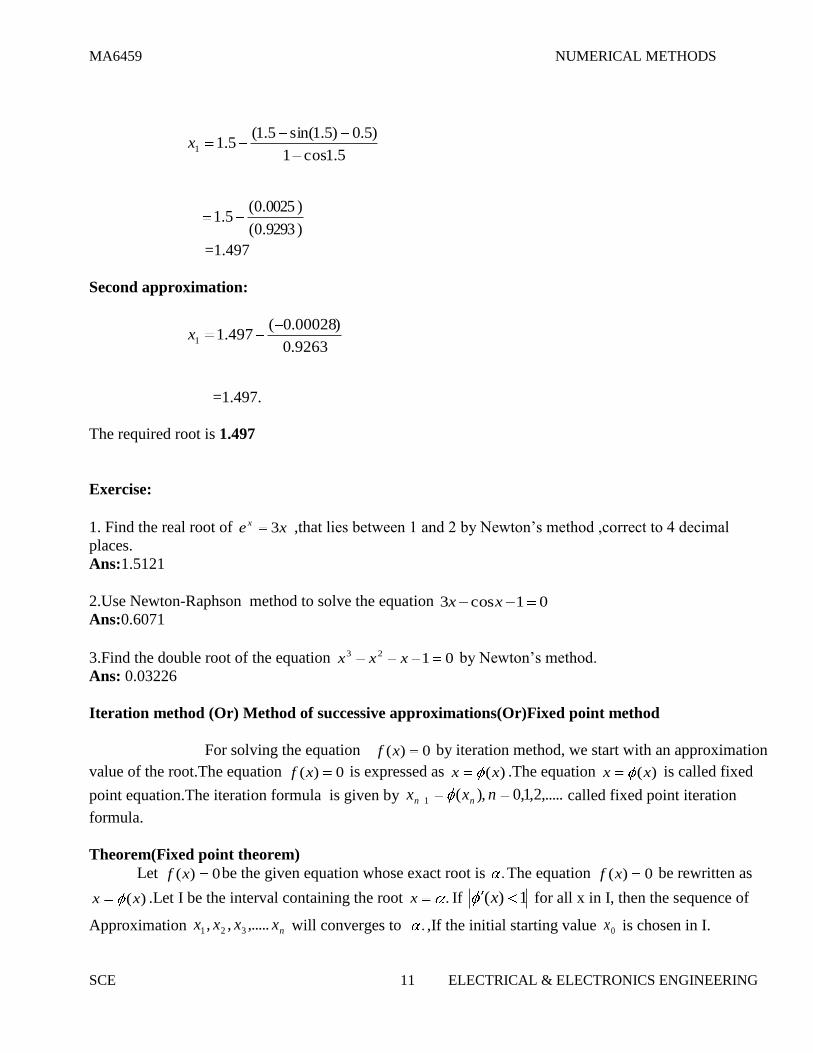
MA6459 NUMERICAL METHODS
SCE 11 ELECTRICAL & ELECTRONICS ENGINEERING
5.1cos1
)5.0)5.1sin(5.1(5.11x
)9293.0(
)0025.0(5.1
=1.497
Second approximation:
9263.0
)00028.0(497.11x
=1.497.
The required root is 1.497
Exercise:
1. Find the real root of xe x 3 ,that lies between 1 and 2 by Newton’s method ,correct to 4 decimal
places.
Ans:1.5121
2.Use Newton-Raphson method to solve the equation 01cos3 xx
Ans:0.6071
3.Find the double root of the equation 0123 xxx by Newton’s method.
Ans: 0.03226
Iteration method (Or) Method of successive approximations(Or)Fixed point method
For solving the equation 0)(xf by iteration method, we start with an approximation
value of the root.The equation 0)(xf is expressed as )(xx .The equation )(xx is called fixed
point equation.The iteration formula is given by ,.....2,1,0),(1 nxx nn called fixed point iteration
formula.
Theorem(Fixed point theorem)
Let 0)(xf be the given equation whose exact root is . The equation 0)(xf be rewritten as
)(xx .Let I be the interval containing the root .x If 1)(x for all x in I, then the sequence of
Approximation nxxxx ,.....,, 321 will converges to . ,If the initial starting value 0x is chosen in I.
MA6459 NUMERICAL METHODS
SCE 12 ELECTRICAL & ELECTRONICS ENGINEERING
The order of convergence
Theorem
Let . be a root of the equation )(xgx .If 0)(0)(,.......0)(,0)( )()1( pp andgggg
.then the convergence of iteration )(1 ii xgx is of order p.
Note
The order of convergence in general is linear (i.e) =1
Problems
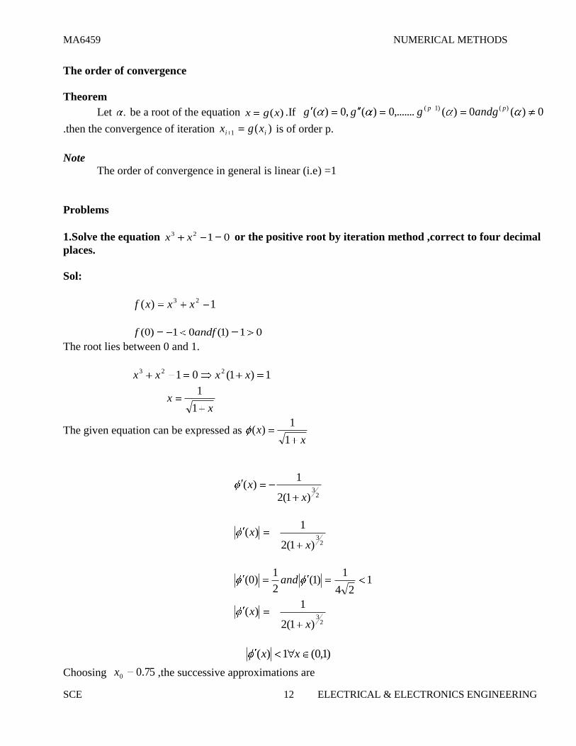
1.Solve the equation 0123 xx or the positive root by iteration method ,correct to four decimal
places.
Sol:
1)( 23 xxxf
01)1(01)0( andff
The root lies between 0 and 1.
1)1(01 223 xxxx
x
x1
1
The given equation can be expressed as x
x1
1)(
23
)1(2
1)(
xx
23
)1(2
1)(
xx
124
1)1(
2
1)0( and
2
3
)1(2
1)(
xx
)1,0(1)( xx
Choosing 75.00x ,the successive approximations are

MA6459 NUMERICAL METHODS
SCE 13 ELECTRICAL & ELECTRONICS ENGINEERING
75.01
11x
=0.75593
75488.0
75488.0
75487.0
75463.0
75465.0
6
5
4
3
2
x
x
x
x
x
Hence the root is 0.7549
Exercise:
1. Find the cube root of 15, correct to four decimal places, by iteration method
Ans: 2.4662
1.2 System of linear equation
Introduction
Many problems in Engineering and science needs the solution of a system of simultaneous linear
equations .The solution of a system of simultaneous linear equations is obtained by the following two
types of methods
Direct methods (Gauss elimination and Gauss Jordan method)
Indirect methods or iterative methods (Gauss Jacobi and Gauss Seidel method)
(a) Direct methods are those in which
The computation can be completed in a finite number of steps resulting in the exact
solution
The amount of computation involved can be specified in advance.
The method is independent of the accuracy desired.
(b) Iterative methods (self correcting methods) are which
Begin with an approximate solution and
Obtain an improved solution with each step of iteration
But would require an infinite number of steps to obtain an exact solution without
round-off errors
The accuracy of the solution depends on the number of iterations performed.

MA6459 NUMERICAL METHODS
SCE 14 ELECTRICAL & ELECTRONICS ENGINEERING
Simultaneous linear equations
The system of equations in n unknowns nxxxx ,.....,, 321 is given by
11212111 .......... bxaxaxa nn
22222121 .......... bxaxaxa nn
…………………………………………………………
………………………………………………………….
………………………………………………………….
nnmnnn bxaxaxa ..........2211
This can be written as BAX where T
n
T
nnnij bbbbBxxxxXaA ,.....,,;,.....,,; 321321
This system of equations can be solved by using determinants (Cramer’s rule) or by means of matrices.
These involve tedious calculations. These are other methods to solve such equations .In this chapter we
will discuss four methods viz.
(i) Gauss –Elimination method
(ii) Gauss –Jordan method
(iii) Gauss-Jacobi method
(iv) Gauss seidel method
Gauss-Elimination method
This is an Elimination method and it reduces the given system of equation to an equivalent upper
triangular system which can be solved by Back substitution.
Consider the system of equations
3333232131
2323222121
1313212111
bxaxaxa
bxaxaxa
bxaxaxa
Gauss-algorithm is explained below:
Step 1. Elimination of 1x from the second and third equations .If ,011a the first equation is
used to eliminate 1x from the second and third equation. After elimination, the reduced system is

MA6459 NUMERICAL METHODS
SCE 15 ELECTRICAL & ELECTRONICS ENGINEERING
3333232
2323222
1313212111
bxaxa
bxaxa
bxaxaxa
Step 2:
Elimination of 2x from the third equation. If ,022a We eliminate 2x from third equation and
the reduced upper triangular system is
3333
2323222
1313212111
bxa
bxaxa
bxaxaxa
Step 3:
From third equation 3x is known. Using 3x in the second equation 2x is obtained. using both
2x And 3x in the first equation, the value of 1x is obtained.
Thus the elimination method, we start with the augmented matrix (A/B) of the given system and
transform it to (U/K) by eliminatory row operations. Finally the solution is obtained by back
substitution process.
Principle
)/()/( lim KUBA inationeGauss
2. Gauss –Jordan method
This method is a modification of Gauss-Elimination method. Here the elimination of unknowns is
performed not only in the equations below but also in the equations above. The co-efficient matrix
A of the system AX=B is reduced into a diagonal or a unit matrix and the solution is obtained
directly without back substitution process.
)/()/()/( KIorKDBA JordanGauss
Examples
1.Solve the equations 33114,20238,1242 zyxzyxzyx by (1)Gauss –Elimination
method (2) Gauss –Jordan method
Sol:

MA6459 NUMERICAL METHODS
SCE 16 ELECTRICAL & ELECTRONICS ENGINEERING
(i)Gauss-Elimination method
The given system is equivalent to BAX where
and
Principle. Reduce to
=
From this ,the equivalent upper triangular system of equations is
1242 zyx
28147 zy
2727z
z=1,y=2,x=3 By back substitution.
The solution is x=3,y=2,z=1
(ii)Gauss –Jordan method
Principle. Reduce to

MA6459 NUMERICAL METHODS
SCE 17 ELECTRICAL & ELECTRONICS ENGINEERING
From this ,we have
y = 2
z=1
Exercise
1. Solve the system by Gauss –Elimination method 532,303,14225 zyxzyxzyx .
Ans: x= 39.3345;y=16.793;z=18.966
2. Solve the equations 40543,13432,9 zyxzyxzyx by (1) Gauss –Elimination
method (2) Gauss –Jordan method
Ans: x=1; y=3; z=5
Iterative method
These methods are used to solve a special of linear equations in which each equation must possess
one large coefficient and the large coefficient must be attached to a different unknown in that
equation.Further in each equation, the absolute value of the large coefficient of the unknown is greater
than the sum of the absolute values of the other coefficients of the other unknowns. Such type of
simultaneous linear equations can be solved by the following iterative methods.
Gauss-Jacobi method
Gauss seidel method

MA6459 NUMERICAL METHODS
SCE 18 ELECTRICAL & ELECTRONICS ENGINEERING
3333
2222
1111
dzcybxa
dzcybxa
dzcybxa
i.e., the co-efficient matrix is diagonally dominant.
Solving the given system for x,y,z (whose diagonals are the largest values),we have
][1
][1
][1
333
3
222
2
111
1
ybxadc
z
zcxadb
y
zcybda
x
Gauss-Jacobi method
If the rth
iterates are )()()( ,, rrr zyx ,then the iteration scheme for this method is
)(1
)(1
)(1
)(
3
)(
33
3
)1(
)(
2
)(
22
2
)1(
)(
1
)(
11
1
)1(
rrr
rrr
rrr
ybxadc
z
zcxadb
y
zcybda
x
The iteration is stopped when the values x, y, z start repeating with the desired degree of accuracy.
Gauss-Seidel method
This method is only a refinement of Gauss-Jacobi method .In this method ,once a new value for a
unknown is found ,it is used immediately for computing the new values of the unknowns.
If the rth
iterates are, then the iteration scheme for this method is
)(1
)(1
)(1
)1(
3
)1(
33
3
)1(
)(
2
)1(
22
2
)1(
)(
1
)(
11
1
)1(
rrr
rrr
rrr
ybxadc
z
zcxadb
y
zcybda
x
Hence finding the values of the unknowns, we use the latest available values on the R.H.S
The process of iteration is continued until the convergence is obtained with desired accuracy.

MA6459 NUMERICAL METHODS
SCE 19 ELECTRICAL & ELECTRONICS ENGINEERING
Conditions for convergence
Gauss-seidel method will converge if in each equation of the given system ,the absolute values o
the largest coefficient is greater than the absolute values of all the remaining coefficients
niaan
jj
ijii .........3,2,11,1
This is the sufficient condition for convergence of both Gauss-Jacobi and Gauss-seidel iteration methods.
Rate of convergence
The rate of convergence of gauss-seidel method is roughly two times that of Gauss-Jacobi method.
Further the convergences in Gauss-Seidel method is very fast in gauss-Jacobi .Since the current values of
the unknowns are used immediately in each stage of iteration for getting the values of the unknowns.
Problems
1.Solve by Gauss-Jacobi method, the following system354172,24103,32428 zyxzyxzyx
Sol:
Rearranging the given system as
24103
354172
32428
zyx
zyx
zyx
The coefficient matrix is is diagonally dominant.
Solving for x,y,z ,we have
We start with initial values =
The successive iteration values are tabulated as follows

MA6459 NUMERICAL METHODS
SCE 20 ELECTRICAL & ELECTRONICS ENGINEERING
Iteration X Y Z
1 1.143 2.059 2.400
2 0.934 1.360 1.566
3 1.004 1.580 1.887
4 0.983 1.508 1.826
5 0.993 1.513 1.849
6 0.993 1.507 1.847
7 0.993 1.507 1.847
X=0.993;y=1.507;z=1.847
2.Solve by Gauss-Seidel method, the following system11054,722156;85627 zyxzyxzyx
Sol:
The given system is diagonally dominant.
Solving for x,y,z, we get
We start with initial values =
The successive iteration values are tabulated as follows
Iteration X Y Z
1 3.148 3.541 1.913
2 2.432 3.572 1.926
3 2.426 3.573 1.926
4 2.425 3.573 1.926
5 2.425 3.573 1.926
X=2.425;y=3.573;z=1.926
Exercise:
1.Solve by Gauss-Seidel method, the following system
780.2;341.1;89.0:
221032,442302;9210
zyxAns
zyxzyxzyx

MA6459 NUMERICAL METHODS
SCE 21 ELECTRICAL & ELECTRONICS ENGINEERING
2.Solve by Gauss-Seidel method and Gauss-Jacobi method, the following system
069.1;798.2;580.2)(541.3;522.1;321.1)(:
48217,301822;753230
zyxiizyxiAns
zyxzyxzyx
1.3 Matrix inversion
Introduction
A square matrix whose determinant value is not zero is called a non-singular matrix. Every non-
singular square matrix has an inverse matrix. In this chapter we shall find the inverse of the non-singular
square matrix A of order three. If X is the inverse of A,
Then
Inversion by Gauss-Jordan method
By Gauss Jordan method, the inverse matrix X is obtained by the following steps:
Step 1: First consider the augmented matrix
Step 2: Reduce the matrix A in to the identity matrix I by employing row transformations.
The row transformations used in step 2 transform I to A-1
Finally write the inverse matrix A-1
.so the principle involved for finding A-1
is as shown below
Note
The answer can be checked using the result
Problems
1.Find the inverse of by Gauss-Jordan method.
Sol:
MA6459 NUMERICAL METHODS
SCE 22 ELECTRICAL & ELECTRONICS ENGINEERING
Thus
Hence
2.Find the inverse of by Gauss-Jordan method
Exercise:
1. Find the inverse of by Gauss-Jordan method.
2.By Gauss-Jordan method ,find 1A if
1.4 Eigen value of a Matrix
Introduction
For every square matrix A, there is a scalar and a non-zero column vector X such that
XAX .Then the scalar is called an Eigen value of A and X, the corresponding Eigen vector. We
have studied earlier the computation of Eigen values and the Eigen vectors by means of analytical method.
In this chapter, we will discuss an iterative method to determine the largest Eigen value and the
corresponding Eigen vector.
Power method (Von Mise’s power method)
Power method is used to determine numerically largest Eigen value and the
corresponding Eigen vector of a matrix A
Working Procedure

MA6459 NUMERICAL METHODS
SCE 23 ELECTRICAL & ELECTRONICS ENGINEERING
(For a square matrix)
Assume the initial vector
Then find
Normalize the vector to get a new vector
(i.e) is the largest component in magnitude of
Repeat steps (2) and (3) till convergence is achieved.
The convergence of mi and Xi will give the dominant Eigen value and the
corresponding Eigen vector X Thus niX
Y
ik
ik........2,1,0,lim
1
1
And is the required Eigen vector.
Problems
1.Use the power method to find the dominant value and the corresponding Eigen vector of
the matrix
Sol:
Let
1 1X
2 2X
3 3X
4 4X

MA6459 NUMERICAL METHODS
SCE 24 ELECTRICAL & ELECTRONICS ENGINEERING
5 5X
Hence the dominant Eigen value is 15.97 and the corresponding Eigen vector is
2. Determine the dominant Eigen value and the corresponding Eigen vector of
Using power method.
Exercise:
1. Find the dominant Eigen value and the corresponding Eigen vector of A Find
also the other two Eigen values.
2. Find the dominant Eigen value of the corresponding Eigen vector of
By power method. Hence find the other Eigen value also.
Tutorial problems
Tutorial 1
1. Determine the real root of 3xxe correct tot four decimal places by Regula falsi method.
Ans:1.0499
2. Solve the equation xtanx=-1 by Regula falsi method ,correct to 4 decimal places
Ans:2.7984
3. Find by Newton’s method , the real root of 2.1log10 xx correct to 4 decimal places
Ans:2.7406
4. Find the double root of the equation 0123 xxx by Newton’s method.
Ans:x=1
5. Solve xx 1tan1 by iteration method ,starting with 20x
Ans:2.1323
Tutorial 2
1.Solve the following system by Gauss-elimination method

MA6459 NUMERICAL METHODS
SCE 25 ELECTRICAL & ELECTRONICS ENGINEERING
2,1,2,1:
64;56;127;45
4321
4321432143214321
xxxxAns
xxxxxxxxxxxxxxxx
2.Solve the system of equation 1224,20432,82 zyxzyxzyx by Gauss-Jordan
method
Ans:x=1,y=2,z=3.
3.Solve the following equations 221032,442302,9210 zyxzyxzyx
By Gauss-Seidel method.
4.Solve by Gauss Jacobi method ,the following 3542,24103,32428 zyxzyxzyx
Ans:x=0.993,y=1.07,z=1.847.
5.Solve the following equations
31932,291043,3043122,183513 4321432143214321 xxxxxxxxxxxxxxxx
By Gauss-Seidel method.
Ans: 163.4,703.3,482.3,58.0 4321 xxxx
Tutorial 3
1.Find the inverse of using Gauss-Jordan method.
Ans:
2.By Gauss-Jordan method ,find A-1
if
Ans:
3.Determine the dominant Eigen value and the corresponding Eigen vector of
using power method.
Ans:[0.062,1,0.062]T
4.Find the smallest Eigen value and the corresponding Eigen vector of
using power method.
Ans:[0.707,1,0.707]T
5.Find the dominant Eigen value and the corresponding Eigen vector of by power
method.Hence find the other Eigen value also .
Ans:λ=2.381

MA6459 NUMERICAL METHODS
SCE 26 ELECTRICAL & ELECTRONICS ENGINEERING
QUESTION BANK
PART A
1. What is the order of convergence of Newton-Raphson methods if the multiplicity of the root is
one.
Sol:
Order of convergence of N.R method is 2
2. Derive Newton’s algorithm for finding the pth
root of a number N.
Sol:
If x= N 1/p
,
Then xp-N = 0 is the equation to be solved.
Let f(x) = xp-N, f’(x) = px
p-1
By N.R rule, if xr is the r th
iterate
Xr+1 = xr -
= xr -
=
=
3. What is the rate of convergence in N.R method?
Sol:
The rate of convergence in N.R method is of order 2
4. Define round off error.
Sol:
The round off error is the quantity R which must be added to the finite representation of a
computed number in order to make it the true representation of that number.
5. State the principle used in Gauss-Jordan method.
Sol:
Coefficient matrix is transformed into diagonal matrix.
6. Compare Gaussian elimination method and Gauss- Jordan method.
Sol:
Gaussian elimination method Gauss- Jordan method
1
2
3
Coefficient matrix is transformed into
upper triangular matrix
Direct method
We obtain the solution by back
substitution method
Coefficient matrix is transformed
into diagonal matrix
Direct method
No need of back substitution method

MA6459 NUMERICAL METHODS
SCE 27 ELECTRICAL & ELECTRONICS ENGINEERING
7. Determine the largest eigen value and the corresponding eigen value vector of the matrix
correct to two decimal places using power method.
Sol:
AX1 = = = 2 = 2X2
AX2 = = = 2 = 2X3
This shows that the largest eigen value = 2
The corresponding eigen value =
8. Write the Descartes rule of signs
Sol:
1) An equation f (x) = 0 cannot have more number of positive roots than there are
changes of sign in the terms of the polynomial f (x) .
2)An equation f (x) = 0 cannot have more number of positive roots than there are
changes of sign in the terms of the polynomial f (x) .
9. Write a sufficient condition for Gauss seidel method to converge .(or)
State a sufficient condition for Gauss Jacobi method to converge.
Sol:
The process of iteration by Gauss seidel method will converge if in each equation of the
system the absolute value of the largest coefficient is greater than the sum of the
absolute values of the remaining coefficients.
10. State the order of convergence and convergence condition for NR method?
Sol:
The order of convergence is 2
Condition of convergence is
11. Compare Gauss Seidel and Gauss elimination method?
Sol:
Gauss Jacobi method Gauss seidel method
1.
2.
3.
Convergence method is
slow
Direct method
Condition for
convergence is the
coefficient matrix
diagonally dominant
The rate of convergence of
Gauss Seidel method is
roughly twice that of Gauss
Jacobi.
Indirect method
Condition for convergence is
the coefficient matrix
diagonally dominant
12) Is the iteration method a self correcting method always?
Sol:
In general iteration is a self correcting method since the round off error is smaller.

MA6459 NUMERICAL METHODS
SCE 28 ELECTRICAL & ELECTRONICS ENGINEERING
13) If g(x) is continuous in [a , b] then under what condition the iterative method x = g(x) has a
unique solution in [a , b].
Sol:
Let x = r be a root of x = g(x) .Let I = [a , b] be the given interval combining the
point x = r. if g′(x) for all x in I, the sequence of approximation x0 , x 1,......x nwill
converge to the root r, provided that the initial approximation x0 is chosen in r.
14) When would we not use N-R method .
Sol:
If x1 is the exact root and x0 is its approximate value of the equation
f (x) = 0.we know that x 1= x0 –
If is small, the error will be large and the computation of the root by
this, method will be a slow process or may even be impossible.
Hence the method should not be used in cases where the graph of the function when it
crosses the x axis is nearly horizontal.
15) Write the iterative formula of NR method.
Sol:
Xn+1 = xn –
Part B
1.Using Gauss Jordan method, find the inverse of the matrix
2.Apply Gauss-seidel method to solve the equations
20x+y-2z=17: 3x+20y-z=-18: 2x-3y+20z=25.
3.Find a positive root of 3x- log 10 X =6, using fixed point iteration method.
4.Determine the largest eigen value and the corresponding eigen vector of the matrix
with (1 0 0)T as the initial vector by power method.
5.Find the smallest positive root of the equation x = sin x correct to 3 decimal places using
Newton-Raphson method.
6.Find all the eigen value and eigen vectors of the matrix using Jacobi method.
7.Solve by Gauss-seidel iterative procedure the system 8x-3y-2z=20: 6x+3y+12z=35: 4x+11y-
z=33.

MA6459 NUMERICAL METHODS
SCE 29 ELECTRICAL & ELECTRONICS ENGINEERING
8.Find the largest eigen value of by using Power method.
9.Find a real root of the equation x3+x
2-1=0 by iteration method.
10.Using Newton’s method, find the real root of x log 10 X=1.2 correct to five decimal places.
11.Apply Gauss elimination method to find the solution of the following system :
2x+3y-z=5: 4x+4y-3z=3: 2x-3y+2z=2.
12.Find an iterative formula to find , where N is a positive number and hence find
13.Solve the following system of equations by Gauss-Jacobi method:
27x+6y-z=85:x+y+54z=110: 6x+15y+2z=35.
14.Find the Newton’s iterative formula to calculate the reciprocal of N and hence find the value of
.
15.Apply Gauss-Jordan method to find the solution of the following system:
10x+y+z=12: 2x+10y+z=13: x+y+5z=7.

MA6459 NUMERICAL METHODS
SCE 30 ELECTRICAL & ELECTRONICS ENGINEERING
CHAPTER 2
INTERPOLATION AND APPROXIMATION
2.1 Interpolation with Unequal intervals
Introduction
Interpolation is a process of estimating the value of a function at ana
intermediate point when its value are known only at certain specified points.It is based on the
following assumptions:
(i) Given equation is a polynomial or it can be represented by a polynomial with a
good degree of approximation.
(ii) Function should vary in such a way that either it its increasing or decreasing in the
given range without sudden jumps or falls of functional values in the given interval.
We shall discuss the concept of interpolation from a set of tabulated values
of when the values of x are given intervals or at unequal intervals
.First we consider interpolation with unequal intervals.
Lagrange’s Interpolation formula
This is called the Lagrange’s formula for Interpolation.
Problems
1. Using Lagrange’s interpolation formula, find the value of y corresponding to x=10
from the following data
X 5 6 9 11
Y 12 13 14 16
Sol:
Given

MA6459 NUMERICAL METHODS
SCE 31 ELECTRICAL & ELECTRONICS ENGINEERING
By Lagrange’s interpolation formula
Using x=10 and the given data,
y (10) =14.67
2. Using Lagrange’s interpolation formula, find the value of y corresponding to x=6 from the
following data
X 3 7 9 10
Y 168 120 72 63
Sol:
Given
By Lagrange’s interpolation formula
Using x=6 and the given data, y(6)=147
3.Apply Lagrange’s formula to find f(5),given that f(1)=2,f(2)=4,f(3)=8 and f(7)=128
Sol:
Given
By Lagrange’s interpolation formula

MA6459 NUMERICAL METHODS
SCE 32 ELECTRICAL & ELECTRONICS ENGINEERING
Using x=5 and the given data, y(5)=32.93
Exercise
1.Find the polynomial degree 3 fitting the following data
X -1 0 2 3
Y -2 -1 1 4
Ans:
2.Given
Ans:
Inverse Interpolation by Lagrange’s interpolating polynomial
Lagrange’s interpolation formula can be used find a value of x corresponding to a given y which
is not in the table. The process of finding such of x is called inverse interpolation.
If x is the dependent variable and y is the independent variable, we can write a formula for
x as a function of y.
The Lagrange’s interpolation formula for inverse interpolation is
Problems
1.Apply Lagrange’s formula inversely to obtain the root of the equation
Given that
Sol:
Given that

MA6459 NUMERICAL METHODS
SCE 33 ELECTRICAL & ELECTRONICS ENGINEERING
To find x such that
Applying Lagrange’s interpolation formula inversely ,we get
=0.8225
2.Given data
x 3 5 7 9 11
y 6 24 58 108 174
Find the value of x corresponding to y=100.
Sol:
Given that
Using the given data and y=100, we get
X=8.656
The value of x corresponding to y=100 is 8.656

MA6459 NUMERICAL METHODS
SCE 34 ELECTRICAL & ELECTRONICS ENGINEERING
2.2 Divided Difference –Newton Divided Difference Interpolation Formula
Introduction
If the values of x are given at unequal intervals, it is convenient to introduce the idea of
divided differences. The divided difference are the differences of y=f(x) defined, taking into
consideration the changes in the values of the argument .Using divided differences of the function
y=f(x),we establish Newton’s divided difference interpolation formula, which is used for
interpolation which the values of x are at unequal intervals and also for fitting an approximate
curve for the given data.
Divided difference
Let the function assume the values
Corresponding to the arguments nxxxx ,.....,, 321 respectively, where the intervals
need to be equal.
Definitions
The first divided difference of f(x) for the arguments is defined by
It is also denoted by [ ]
Similarly for arguments and so on.
The second divided differences of f(x) for three arguments 210 ,, xxx
Is defined as
The third divided difference of f(x) for the four arguments 3210 ,,, xxxx
Is defined as
And so on .

MA6459 NUMERICAL METHODS
SCE 35 ELECTRICAL & ELECTRONICS ENGINEERING
Representation by Divided difference table
Arguments
Entry First Divided difference Second D-D
Third D-D
Properties of divided difference
The divided differences are symmetrical in all their arguments.
The operator is linear.
The nth
divided differences of a polynomial of nth
degree are constants.
Problems
1.If find the divided difference
Sol:
=

MA6459 NUMERICAL METHODS
SCE 36 ELECTRICAL & ELECTRONICS ENGINEERING
=
=
2.Find the third differences with arguments 2,4,9,10 for the function
Newton’s Divided difference Formula (Or) Newton’s Interpolation Formula for unequal
intervals
Problems
1.Find the polynomial equation passing through(-1,3),(0,-6),(3,39),(6,822),(7,1611)
Sol:
Given data
x -1 0 3 6 7
y 3 -6 39 822 1611
The divided difference table is given as follows
-1
0
3
6
7
3
-6
39
822
1611
-9
15
261
789
6
41
132
5
13
1

MA6459 NUMERICAL METHODS
SCE 37 ELECTRICAL & ELECTRONICS ENGINEERING
By Newton’s formula,
Is the required polynomial.
2. Given the data
Find the form of the function .Hence find f(3).
Ans: f(3)=35
2.3 Interpolating with a cubic spline-cubic spline Interpolation
We consider the problem of interpolation between given data points (xi, yi),
i=0, 1, 2, 3….n where a= bxxxx n.....321 by means of a smooth polynomial curve.
By means of method of least squares, we can fit a polynomial but it is appropriate.”Spline fitting”
is the new technique recently developed to fit a smooth curve passing he given set of points.
Definition of Cubic spline
A cubic spline s(x) is defined by the following properties.
S(xi)=yi,i=0,1,2,…..n
S(x),s’(x),s”(x) are continuous on [a,b]
S(x) is a cubic polynomial in each sub-interval(xi,xi+1),i=0,1,2,3…..n=1
Conditions for fitting spline fit
The conditions for a cubic spline fit are that we pass a set of cubic through the
points, using a new cubic in each interval. Further it is required both the slope and the curvature be
the same for the pair of cubic that join at each point.
x 0 1 2 5
f(x) 2 3 12 147

MA6459 NUMERICAL METHODS
SCE 38 ELECTRICAL & ELECTRONICS ENGINEERING
Natural cubic spline
A cubic spline s(x) such that s(x) is linear in the intervals ),(),( 1 nxandx
i.e. s1=0 and sn=0 is called a natural cubic spline
where 1s =second derivative at ),( 11 yx
ns Second derivative at ),( nn yx
Note
The three alternative choices used are
01s and 0ns i.e. the end cubics approach linearity at their extremities.
121 ; nn ssss i.e. the end cubics approaches parabolas at their extremities
Take 1s as a linear extrapolation from 2s and nandss3 is a linear extrapolation from 21 nn andss
.with the assumption, for a set of data that are fit by a single cubic equation their cubic
splines will all be this same cubic
For equal intervals ,we have hhh ii 1 ,the equation becomes
]2[6
4 11211 iiiiii yyyh
sss for i=1,2,3,….n-1
Problems
1.Fit a natural cubic spline to the following data
x 1 2 3
y -8 -1 18
And compute (i) y(1.5) (ii) y’(1)
Solution
Here n=2 ,the given data )18,3(),(),1,2(),(),8,1(),( 332211 yxyxyx
For cubic natural spline, 0&0 31 ss .The intervals are equally spaced.
For equally spaced intervals,the relation on 321 &, sss is given by
]2[1
64 3212321 yyysss ]1[ h
182s
For the interval ]2[21 1 xxx ,the cubic spline is given by
111
2
11
3
11 )()()( dxxcxxbxxay

MA6459 NUMERICAL METHODS
SCE 39 ELECTRICAL & ELECTRONICS ENGINEERING
The values of 1111 ,,, dcba are given by
]1[ ih
8,4,0,3 1111 dcba
The cubic spline for the interval 21 x is
8
45)5.1()5.1(
8)14(4)1(3)( 3
sy
xxxs
The first derivative of s(x) is given by
)(1
)2(6
)( 111
ii
i
iii yyh
ssh
xs
Taking i=1, )()2(6
1)1( 1221 yysss ]1[ ih
4)1(s
4)1(y
We note that the tabulated function is 93xy and hence the actual values of )5.1(y and )1(y
are respectively8
45and 3.
2.The following values of x and y are given ,obtain the natural cubic spline which agree with
y(x) at the set of data points
x 2 3 4
y 11 49 123
Hence compute (i) y(2.5) and (ii) )2(y
Exercise:
1.Fit the following data by a cubic spline curve
x 0 1 2 3 4
y -8 -7 0 19 56
Using the end condition that 51 & ss are linear extrapolations.
1121
1211
112
1 ),6
2()(,
2,
6yd
ssyyc
sb
ssa

MA6459 NUMERICAL METHODS
SCE 40 ELECTRICAL & ELECTRONICS ENGINEERING
2.Fit a natural cubic spline to 251
20)(
xxf on the interval [-2,-1].Use five equispaced points of
the function at x=-2(1)2.hence find y(1.5).
2.4 Interpolation with equal intervals
(Newton’s Forward and Backward Difference formulas)
Introduction
If a function y=f(x) is not known explicitly the value of y can be obtained when s set of
values of ii yx , i=1,2,3….n are known by using methods based on the principles of finite
differences ,provided the function y=f(x) is continuous.
Assume that we have a table of values ii yx , i=1,2,3….n of any function, the values of x being
equally spaced, niihxxei i ,....2,1,0,.,. 0
Forward differences
If nyyyy ,......,, 210 denote a set of values of y,then the first forward differences of y=f(x)
are defined by 11121010 .;.........; nnn yyyyyyyyy
Where is called the forward difference operator.
Backward differences
The differences 01 yy , 12 yy ,……….. 1nn yy are called first backward
differences and they are denoted by 9.2ny 1122011 .;.........; nnn yyyyyyyyy
Where is called the backward difference operator.In similar way second, third and higher order
backward differences are defined.
........;.........; 344
2
233
2
122
2 yyyyyyyyy
3
2
4
2
4
3
2
2
3
2
3
3 ; yyyyyy and so on.
Fundamental Finite Difference operators
Forward Difference operator ( 010 yyy )
If =f(x) then )()( xfhxfy
Where h is the interval of differencing
Backward Difference operator ( 011 yyy )
The operator is defined by )()()( hxfxfxf
Shift operator
The shift operator is defined by 1rr yEy
i.e the effect of E is to shift functional value ry to the next value 1ry .Also 2
2
rr yyE

MA6459 NUMERICAL METHODS
SCE 41 ELECTRICAL & ELECTRONICS ENGINEERING
In general rnr
n yyE
The relation between and E is given by
1)(1 EorE
Also the relation between and E-1
is given by
11 E
Newton’s Forward Interpolation formula
Let y=f(x) be a function which takes the values nyyyy ,......,, 210 corresponding to
the values nxxxx ,......,, 210 where the values of x are equally spaced.
i.e. niihxxi ,.......,2,1,0,0
h
xxp
pppy
ppypyy p
0
0
2
00 ...........!3
)2)(1(
!2
)1(
This formula is called Newton-Gregory forward interpolation formula.
Newton’s Backward Interpolation formula
This formula is used for interpolating a value of y for given x near the end of a table
of values .Let nyyyy ,......,, 210 be the values of y =f(x) for nxxxxx ,......,, 210 where
niihxxi ,.......,2,1,0,0
......!3
)2)(1(
!2
)1()( 32
nnnnn yppp
ypp
ypyphxy
h
xxp n
This formula is called Newton Backward interpolation formula.
We can also use this formula to extrapolate the values of y, a short distance ahead of yn.

MA6459 NUMERICAL METHODS
SCE 42 ELECTRICAL & ELECTRONICS ENGINEERING
Problems
1.Using Newton’s Forward interpolation formula ,find f(1.02) from the following data
X 1.0 1.1 1.2 1.3 1.4
F(x) 0.841 0.891 0.932 0.964 0.985
Sol:
Forward difference table:
x )(xfy
y
y2
y3
1.0
1.1
1.2
1.3
1.4
0.841
0.891
0.932
0.964
0.985
0.050
0.041
0.032
0.021
-0.009
-0.009
-0.011
0
-0.002
009.0,050.0,841.0 0
2
00 yyy
Let 02.1&0.10 xx
h
xxp 0
2.0p
By Newton’s Forward interpolation formula,
.........!2
)1()02.1( 0
2
00 ypp
ypyy
=0.852
)02.1(y =0.852
2.Using Newton’s Forward interpolation formula, find the value of sin52 given that
.8660.060sin,8192.055sin,7660.050sin,7071.045sin 0000Ans:0.7880
3.Using Newton’s Backward interpolation formula, find y when x=27,from the following data
x 10 15 20 25 30
y 35.4 32.2 29.1 26.0 23.1

MA6459 NUMERICAL METHODS
SCE 43 ELECTRICAL & ELECTRONICS ENGINEERING
Sol:
Backward difference table
x y
y y2
y3
y4
10
15
20
25
30
35.4
32.2
29.1
26.0
23.1
-3.2
-3.1
-3.1
-2.9
0.1
0
0.2
-0.1
0.2
0.3
Here ,1.23,30 nn yx 9.2ny ,2.02
ny 2.03
ny , 3.04
ny
By Newton’s backward interpolation formula,
......!3
)2)(1(
!2
)1()( 32
nnnnn yppp
ypp
ypyphxy
Here x=27,h
xxp n
6.0p
y(27)=24.8
4.Find the cubic polynomial which takes the value y(0)=1,y(1)=0,y(2)=1,y(3)=10.Hence or
otherwise ,obtain y(4).Ans:y(4)=33
Exercise:
1.Given the data
x 0 1 2 3 4
y 2 3 12 35 78
Find the cubic function of x,using Newton’s backward interpolation formula.
Ans: 2)( 23 xxxxy
2.Using Newton’s Gregory backward formula, find 9.1e from the following data
x 1.00 1.25 1.50 1.75 2.00 xe 0.3679 0.2865 0.2231 0.1738 0.1353

MA6459 NUMERICAL METHODS
SCE 44 ELECTRICAL & ELECTRONICS ENGINEERING
Ans: 9.1e =0.1496
3.Estimate exp(1.85) from the following table using Newton’s Forward interpolation formula
x 1.7 1.8 1.9 2.0 2.1 2.2 2.3 xe 5.474 6.050 6.686 7.839 8.166 9.025 9.974
Ans:6.3601
4.Find the polynomial which passes through the points (7,3)(8,1)(9,1)(10,9)using Newton’s
interpolation formula.
Tutorial Problems
Tutorial 1
1.Apply Lagrange’s formula inversely to obtain the root of the equation f(x)=0,given that
f(0)=-4,f(1)=1,f(3)=29,f(4)=52.
Ans: 0.8225
2.Using Lagrange’s formula of interpolation ,find y(9.5) given the data
X 7 8 9 10
Y 3 1 1 9
Ans: 3.625
3.Use Lagrange’s formula to find the value of y at x=6 from the following data
x 3 7 9 10
y 168 120 72 63
Ans: 147
4.If log(300)=2.4771,log(304)=2.4829,log(305)=2.4843,log(307)=2.4871find log(301)
Ans: 2.8746
5. Given Finduuuu ..15,33,9,6 7310 2u
Ans:9

MA6459 NUMERICAL METHODS
SCE 45 ELECTRICAL & ELECTRONICS ENGINEERING
Tutorial 2
1.Given the data
x 0 1 2 5
F(x) 2 3 12 147
Find the form of the function. Hence find f(3).Ans:35
2.Find f(x) as a polynomial in powers of(x-5) given the following table
X 0 2 3 4 7 9
Y 4 26 58 112 466 922
Ans: 194)5(98)5(17)5()( 23 xxxxf
3.from the following table,find f(5)
X 0 1 3 6
F(x) 1 4 88 1309
Ans:676
4.Fit the following data by a cubic spline curve
X 0 1 2 3 4
Y -8 -7 0 19 56
Using the end condition that s1 and s5 are linear extrapolations.
Ans:-8
5.Given the data
X 1 2 3 4
Y 0.5 0.333 0.25 0.20
Find y(2.5) using cubic spline function.
Ans:0.2829
Tutorial 3
1.from the following table,find the number of students who obtained less than 45 marks
Marks 30-40 40-50 50-60 60-70 70-80
No of students 31 42 51 35 31
Ans:48
2.Find tan(0.26) from the following valuesof tanx for 30.010.0 x
X 0.10 0.15 0.20 0.25 0.30
Tanx 0.1003 0.1511 0.2027 0.2553 03093
Ans:0.2662
3.Using newton’s interpolation formula find (i) y when x=48 (ii) y when x=84 from the following
data
X 40 50 60 70 80 90
Y 184 204 226 250 276 304
Ans:199.84,286.96

MA6459 NUMERICAL METHODS
SCE 46 ELECTRICAL & ELECTRONICS ENGINEERING
4.Find the value of f(22) and f(42) from the following data
X 20 25 30 35 40 45
F(x) 354 332 291 260 231 204
Ans:352,219
5.Estimate 038sin from the following data given below
x 0 10 20 30 40
sinx 0 0.1736 0.3240 0.5000 0.6428
Ans:12.7696
Question Bank
Part A
1. State the Lagrange’s interpolation formula.
Sol: Let y = f(x) be a function which takes the values y0, y1,……yn corresponding to
x=x0,x1,……xn
Then Lagrange’s interpolation formula is
Y = f(x) = yo
+ y1
+ ………+ yn
2. What is the assumption we make when Lagrange’s formula is used?
Sol:
Lagrange’s interpolation formula can be used whether the values of x, the independent
variable are equally spaced or not whether the difference of y become smaller or not.
3. When Newton’s backward interpolation formula is used.
Sol:
The formula is used mainly to interpolate the values of y near the end of a set of tabular
values and also for extrapolation the values of y a short distance ahead of y0
4. What are the errors in Trapezoidal rule of numerical integration?
Sol:
The error in the Trapezoidal rule is
E< y”
5. Why Simpson’s one third rule is called a closed formula?

MA6459 NUMERICAL METHODS
SCE 47 ELECTRICAL & ELECTRONICS ENGINEERING
Sol:
Since the end point ordinates y0 and yn are included in the Simpson’s 1/3 rule, it is called
closed formula.
6. What are the advantages of Lagrange’s formula over Newton’s formula?
Sol:
The forward and backward interpolation formulae of Newton can be used only when the
values of theindependent variable x are equally spaced and can also be used when the differences
of the dependent variable y become smaller ultimately. But Lagrange’s interpolation formula can
be used whether the values of x, the independent variable are equally spaced or not and whether
the difference of y become smaller or not.
7. When do we apply Lagrange’s interpolation?
Sol:
Lagrange’s interpolation formula can be used when the values of “x” are equally spaced or
not. It is mainly used when the values are unevenly spaced.
8. When do we apply Lagrange’s interpolation?
Sol:
Lagrange’s interpolation formula can be used when the values of “x” are equally spaced or
not. It is mainly used when the values are unevenly spaced.
9. What are the disadvantages in practice in applying Lagrange’s interpolation formula?
Sol:
1. It takes time.
2. It is laborious
10. When Newton’s backward interpolation formula is used.
Sol:
The formula is used mainly to interpolate the values of ‘y’ near the end of a set of tabular
values.
11. When Newton’s forward interpolation formula is used.
Sol:
The formula is used mainly to interpolate the values of ‘y’ near the beginnig of a set of
tabular values.
12. When do we use Newton’s divided differences formula?
Sol: This is used when the data are unequally spaced.
13. Write Forward difference operator.
Sol:
Let y = f (x) be a function of x and let of the values of y. corresponding to
of the values of x. Here, the independent variable (or argument), x
proceeds at equally spaced intervals and h (constant),the difference between two consecutive
values of x is called the interval of differencing. Now the forward difference operator is defined as

MA6459 NUMERICAL METHODS
SCE 48 ELECTRICAL & ELECTRONICS ENGINEERING
=
=
......................
=
These are called first differences.
14.Write Backward difference operator.
Sol:
The backward difference operator is defined as
=
For n=0,1,2 …
=
=
=
………………….
These are called first differences
Part B
1.Using Newton’s divided difference formula, find f(x) from the following data and hence find
f(4).
x 0 1 2 5
f(x) 2 3 12 147
.
2.Find the cubic polynomial which takes the following values:
x 0 1 2 3
f(x) 1 2 1 10
3.The following values of x and y are given:
x 1 2 3 4
f(x) 1 2 5 11
Find the cubic splines and evaluate y(1.5) and y’(3).
4.Find the rate of growth of the population in 1941 and 1971 from the table below.
Year X 1931 1941 1951 1961 1971
Population
Y
40.62 60.8 79.95 103.56 132.65
5.Derive Newton’s backward difference formula by using operator method.
6.Using Lagrange’s interpolation formula find a polynomial which passes the points
(0,-12),(1,0),(3,6),(4,12).

MA6459 NUMERICAL METHODS
SCE 49 ELECTRICAL & ELECTRONICS ENGINEERING
7.Using Newton’s divided difference formula determine f(3) from the data:
x 0 1 2 4 5
f(x) 1 14 15 5 6
8.Obtain the cubic spline approximation for the function y=f(x) from the following data, given that
y0” = y3”=0.
x -1 0 1 2
y -1 1 3 35
9.The following table gives the values of density of saturated water for various temperatures of
saturated steam.
Temperature 0
C
100 150 200 250 300
Density hg/m3 958 917 865 799 712
Find by interpolation, the density when the temperature is 2750 .
10.Use Lagrange’s method to find log 10 656 , given that log 10 654 =2.8156,
log 10 658 =2.8182 , log 10 659 =2.8189 and log 10 661 =2.8202.
11.Find f’(x) at x=1.5 and x=4.0 from the following data using Newton’s formulae for
differentiation.
x 1.5 2.0 2.5 3.0 3.5 4.0
Y=f(x) 3.375 7.0 13.625 24.0 38.875 59.0
12.If f(0)=1,f(1)=2,f(2)=33 and f(3)=244. Find a cubic spline approximation, assuming
M(0)=M(3)=0.Also find f(2.5).
13.Fit a set of 2 cubic splines to a half ellipse described by f(x)= [25-4x2]1/2
. Choose the three data
points (n=2) as (-2.5,0), (0,1.67) and (2.5 , 0) and use the free boundary conditions.
14.Find the value of y at x=21 and x=28 from the data given below
x 20 23 26 29
y 0.3420 0.3907 0.4384 0.4848
15. The population of a town is as follows:
x year
1941 1951 1961 1971 1981 1991
y population
(thousands)
20 24 29 36 46 51
Estimate the population increase during the period 1946 to1976.

MA6459 NUMERICAL METHODS
SCE 50 ELECTRICAL & ELECTRONICS ENGINEERING
CHAPTER 3
NUMERICAL DIFFERENTIATION AND INTEGRATION
Introduction
Numerical differentiation is the process of computing the value of
For some particular value of x from the given data (xi,yi), i=1, 2, 3…..n where y=f(x) is not known
explicitly. The interpolation to be used depends on the particular value of x which derivatives are
required. If the values of x are not equally spaced, we represent the function by Newton’s divided
difference formula and the derivatives are obtained. If the values of x are equally spaced, the
derivatives are calculated by using Newton’s Forward or backward interpolation formula. If the
derivatives are required at a point near the beginning of the table, we use Newton’s Forward
interpolation formula and if the derivatives are required at a point near the end of table. We use
backward interpolation formula.
3.1 Derivatives using divided differences
Principle
First fit a polynomial for the given data using Newton’s divided difference interpolation
formula and compute the derivatives for a given x.
Problems
1.Compute )4()5.3( fandf given that f(0)=2,f(1)=3;f(2)=12 and f(5)=147
Sol:
Divided difference table
x f f2
1 f3
1
0
1
2
5
2
3
12
147
1
9
45
4
9
1
Newton’s divided difference formula is

MA6459 NUMERICAL METHODS
SCE 51 ELECTRICAL & ELECTRONICS ENGINEERING
.......),,())((),()()()( 210101000 xxxfxxxxxxfxxxfxf
Here ,2)(,2;,1;0 0210 xfxxx ),( 10 xxf =1, 1),,,(;4),,( 3210210 xxxxfxxxf
2)( 23 xxxxf
26)(
123)( 2
xxf
xxxf
.26)4(,75.42)5.3( ff
2.Find the values )5()5( fandf using the following data
x 0 2 3 4 7 9
F(x) 4 26 58 112 466 22
Ans: 98 and 34.
3.1.1 Derivatives using Finite differences
Newton’s Forward difference Formula
........]..........2
3[
1
........]12
11[
1
.......]432
[1
0
4
0
3
33
3
0
4
0
3
0
2
22
2
0
4
0
3
0
2
0
0
0
0
yyhdx
yd
yyyhdx
yd
yyyy
hdx
dy
xx
xx
xx
Newton’s Backward difference formula
........]..........2
3[
1
...]..........12
11[
1
]..........432
[1
43
33
3
432
22
2
432
nn
xx
nnn
xx
nnn
n
xx
yyhdx
yd
yyyhdx
yd
yyyy
hdx
dy
n
n
n

MA6459 NUMERICAL METHODS
SCE 52 ELECTRICAL & ELECTRONICS ENGINEERING
Problems
1.Find the first two derivatives of y at x=54 from the following data
x 50 51 52 53 54
y 3.6840 3.7083 3.7325 3.7563 3.7798
Sol:
Difference table
x
y
y
y2
y3
y4
50
51
52
53
54
3.6840
3.7083
3.7325
3.7563
3.7798
0.0244
0.0241
0.0238
0.0235
-0.0003
-0.0003
-0.0003
0
0
0
By Newton’s Backward difference formula
]..........432
[1
432
nnnn
xx
yyyy
hdx
dy
n
Here h=1; ny =0.0235; 0003.02
ny
02335.054xdx
dy
............12
11[
1 432
2
54
2
2
nnn
x
yyyhdx
yd
=-0.0003

MA6459 NUMERICAL METHODS
SCE 53 ELECTRICAL & ELECTRONICS ENGINEERING
2.Find first and second derivatives of the function at the point x=12 from the following data
x 1 2 3 4 5
y 0 1 5 6 8
Sol:
Difference table
x
y
y
y2
y3
y4
1
2
3
4
5
0
1
5
6
8
1
4
1
2
3
-3
1
-6
4
10
We shall use Newton’s forward formula to compute the derivatives since x=1.2 is at the
beginning.
For non-tabular value phxx 0 ,we have
.......12
31192
6
263
2
12[
10
423
0
32
0
2
0 yppp
ypp
yp
yhdx
dy
Here 0x =1, h=1, x=1.2
2.0
0
p
h
xxp
17.14
773.1
2.1
2
2
2.1
x
x
dx
yd
dx
dy

MA6459 NUMERICAL METHODS
SCE 54 ELECTRICAL & ELECTRONICS ENGINEERING
Exercise:
1.Find the value of 031sec using the following data
x 31 32 33 34
Tanx 0.6008 0.6249 0.6494 0.6745
Ans:1.1718
2.Find the minimum value of y from the following table using numerical differentiation
x 0.60 0.65 0.70 0.75
y 0.6221 0.6155 0.6138 0.6170
Ans: minimum y=0.6137
3.2 Numerical integration
(Trapezoidal rule & Simpson’s rules, Romberg integration)
Introduction
The process of computing the value of a definite integral from a set of values
(xi,yi),i=0,1,2,….. Where 0x =a; bxn of the function y=f(x) is called Numerical integration.
Here the function y is replaced by an interpolation formula involving finite differences and then
integrated between the limits a and b, the value is found.
General Quadrature formula for equidistant ordinates
(Newton cote’s formula)
On simplification we obtain
.......]24
)2(
12
)32(
2[ 0
32
0
2
00
0
ynn
ynn
yn
ynhydxnx
x
This is the general Quadrature formula
By putting n=1, Trapezoidal rule is obtained
By putting n=2, Simpson’s 1/3 rule is derived
By putting n=3, Simpson’s 3/8 rule is derived.
Note
The error in Trapezoidal rule is of order h2 and the total error E is given by y”( )
is the largest of y.
Simpson’s 1/3 rule
)]......(2)......(4)[(3
264215310
0
n
x
x
nn yyyyyyyyyyh
ydxn

MA6459 NUMERICAL METHODS
SCE 55 ELECTRICAL & ELECTRONICS ENGINEERING
Error in Simpson’s 1/3 rule
The Truncation error in Simpson’s 13 rule is of order h4 and the total error is given by
)()(180
)( 4 xwhereyxyhab
E iviv is the largest of the fourth derivatives.
Simpson’s 3/8 rule
......)](2......)(3)[(8
39634210
0
yyyyyyyyh
ydxnx
x
n
Note
The Error of this formula is of order h5 and the dominant term in the error is given by
)(80
3 5 xyh iv
Romberg’s integration
A simple modification of the Trapezoidal rule can be used to find a better approximation to
the value of an integral. This is based on the fact that the truncation error of the Trapezoidal rule is
nearly proportional to h2.
2
1
2
2
2
12
2
21
hh
hIhII
This value of I will be a better approximation than I1 or I2.This method is called Richardson’s
deferred approach to the limit.
If h1=h and h2=h/2,then we get
3
4)
2,( 12 IIh
hI
Problems
1.Evaluate 0
sin xdx by dividing the interval into 8 strips using (i) Trapezoidal rule
(ii) Simpson’s 1/3 rule
Sol:
For 8 strips ,the values of y=sinx are tabulated as follows :
x 0
8
4
8
3
2
8
5
4
3
8
7
sinx 0 0.3827 0.7071 0.9239 1 0.9239 0.7071 0.3827 0
(i)Trapezoidal rule

MA6459 NUMERICAL METHODS
SCE 56 ELECTRICAL & ELECTRONICS ENGINEERING
0
sin xdx = ]2)9239.07071.03827.0(4[16
=1.97425
(ii)Simpson’s 1/3 rule
0
sin xdx = )]7071.017071.0(2)03827923.023.03827.0(4[24
=2.0003
2..Find
1
0
21 x
dx
by using Simpsons 1/3 and 3/8 rule. Hence obtain the approximate value of π
in each case.
Sol:
We divide the range (0,1) into six equal parts, each of size h=1/6.The values of 21
1
xy
at each
point of subdivision are as follows.
x 0 1/6 2/6 3/6 4/6 5/6 1
y 1 0.9730 0.9 0.8 0.623 0.5902 0.5
By Simpson’s 1/3 rule,
)](2)(4)[(31
4253160
1
0
2yyyyyyy
h
x
dx
)]5923.1(2)3632.2(45.1[18
1
=0.7854 (1)
By Simpson’s 3/8 rule,
]2)(3)[(8
3
13542160
1
0
2yyyyyyy
h
x
dx
]6.1)1555.3(35.1[16
1
=0.7854 (2)
But )0(tan)1(tan)(tan
1
111
0
1
1
0
2x
x
dx

MA6459 NUMERICAL METHODS
SCE 57 ELECTRICAL & ELECTRONICS ENGINEERING
From equation (1) and (2), we have ,
π=3.1416
Exercise
1.Evaluate dxe x
2.1
0
2
using (i) Simpson’s 1/3 rule (ii) Simpson’s 3/8 rule ,taking h=0.2
Ans:
(i) dxe x
2.1
0
2
=0.80675 (ii) dxe x
2.1
0
2
=0.80674
2. Evaluate 0
cosxdx by dividing the interval into 8 strips using (i) Trapezoidal rule
(ii) Simpson’s 1/3 rule
Romberg’s method
Problems
1. Use Romberg’s method, to compute
1
0x1
dxI correct to 4 decimal places. Hence find
2log e
Sol:
The value of I can be found by using Trapezoidal rule with=0.5, 0.25, 0.125
(i) h=0.5 the values of x and y are tabulated as below:
x 0 0.5 1
y 1 0.6667 0.5
Trapezoidal rule gives
)]6667.0(25.1[
4
1I
=0.7084
(i) h=0.25, the tabulated values of x and y are as given below:
x 0 0.25 0.5 0.75 1
y 1 0.8 0.6667 0.5714 0.5
Trapezoidal rule gives
)]5714.06667.08.0(25.1[8
1I
=0.6970
(ii) h=0.125 , , the tabulated values of x and y are as given below:

MA6459 NUMERICAL METHODS
SCE 58 ELECTRICAL & ELECTRONICS ENGINEERING
x 0 0.125 0.250 0.375 0.5 0.625 0.750 0.875 1
y 1 0.8889 0.8 0.7273 0.6667 0.6154 0.5714 0.5333 0.5
Trapezoidal rule gives,
)]5333.05714.06154.06667.07273.08.08889.0(25.1[16
1I
=0.6941
We have approximations for I as I1=0.7084,I2=0.6970,I3=0.6941
Use Romberg’s method,the better approximation are caluculated as follws
Using 3
122
IIII
6932.0)2
,(h
hI
6931.0)4
,2
(hh
I
6931.0)4
,2
,(hh
hI
By actual integration,
2log)1(logx1
dx 1
0
1
0
ee xI
2log e =0.6931
2.Use Romberg’s method ,evaluate 0
sin xdx ,correct to four decimal places.
Ans:I=1.9990
Exercise:
1.Use Romberg’s method to compute correct to 4 decimal places.Hence find an
approximate value of
Ans:3.1416
3.3 Gaussian Quadrature
For evaluating the integral
b
a
dxxfI )( ,we derived some integration rules
which require the values of the function at equally spaced points of the interval. Gauss derived
formula which uses the same number of function values but with the different spacing gives better
accuracy.
Gauss’s formula is expressed in the form )(......)()()( 2
1
1
211 nn uFwuFwuFwduuF
=n
i
ii uFw1
)(

MA6459 NUMERICAL METHODS
SCE 59 ELECTRICAL & ELECTRONICS ENGINEERING
Where iw and iu are called the weights and abscissa respectively. In this formula, the abscissa
and weights are symmetrical with respect to the middle of the interval.
The one-point Gaussian Quadrature formula is given by
)0(2)(
1
1
fdxxf , which is exact for polynomials of degree upto 1.
Two point Gaussian formula
)]3
1()
3
1([)(
1
1
ffdxxf
And this is exact for polynomials of degree upto 3.
Three point Gaussian formula
)]5
3()
5
3([
9
5)0(
9
8)(
1
1
fffdxxf
Which is exact for polynomials of degree upto 5
Note:
Number of
terms
Values of t Weighting
factor
Valid upto
degree
2
T=3
1&
3
1
-0.57735&
0.57735
1&1
3
3
7746.05
3
7746.05
3
5555.09
5
8889.09
8
5555.09
5
5
Error terms
The error in two –point Gaussian formula= )(135
1 ivf and the error in three point Gaussian
formula is= )(15750
1 vif
Note

MA6459 NUMERICAL METHODS
SCE 60 ELECTRICAL & ELECTRONICS ENGINEERING
The integral
b
a
dttF )( ,can be transformed into
1
1
)( dxxf by h line transformation
)(2
1)(
2
1abxabt
Problems
1.Evaluate
1
1
21 x
dx by two point and three point Gaussian formula and compare with the
exact value.
Sol:
By two –point Gaussian formula,
)]3
1()
3
1([)(
1
1
ffdxxf
1
1
21 x
dx=1.5
By three-point Gaussian formula
)]5
3()
5
3([
9
5)0(
9
8)(
1
1
fffdxxf
1
1
21 x
dx=1.5833
But exact value= 5708.12
][tan21
2 1
0
1
1
0
2x
x
dx
2.Evaluate
1
1
4
2
1 x
dxx by using Gaussian three point formula
Sol:
Here 4
2
1)(
x
dxxxf
By three-point Gaussian formula
)]5
3()
5
3([
9
5)0(
9
8)(
1
1
fffdxxf …………(1)
MA6459 NUMERICAL METHODS
SCE 61 ELECTRICAL & ELECTRONICS ENGINEERING
34
15)
5
3(f
34
15)
5
3(f
By equation (1),
)]5
3()
5
3([
9
5)0(
9
8)(
1
1
fffdxxf
=21
25
1
1
4
2
1 x
dxx=0.4902
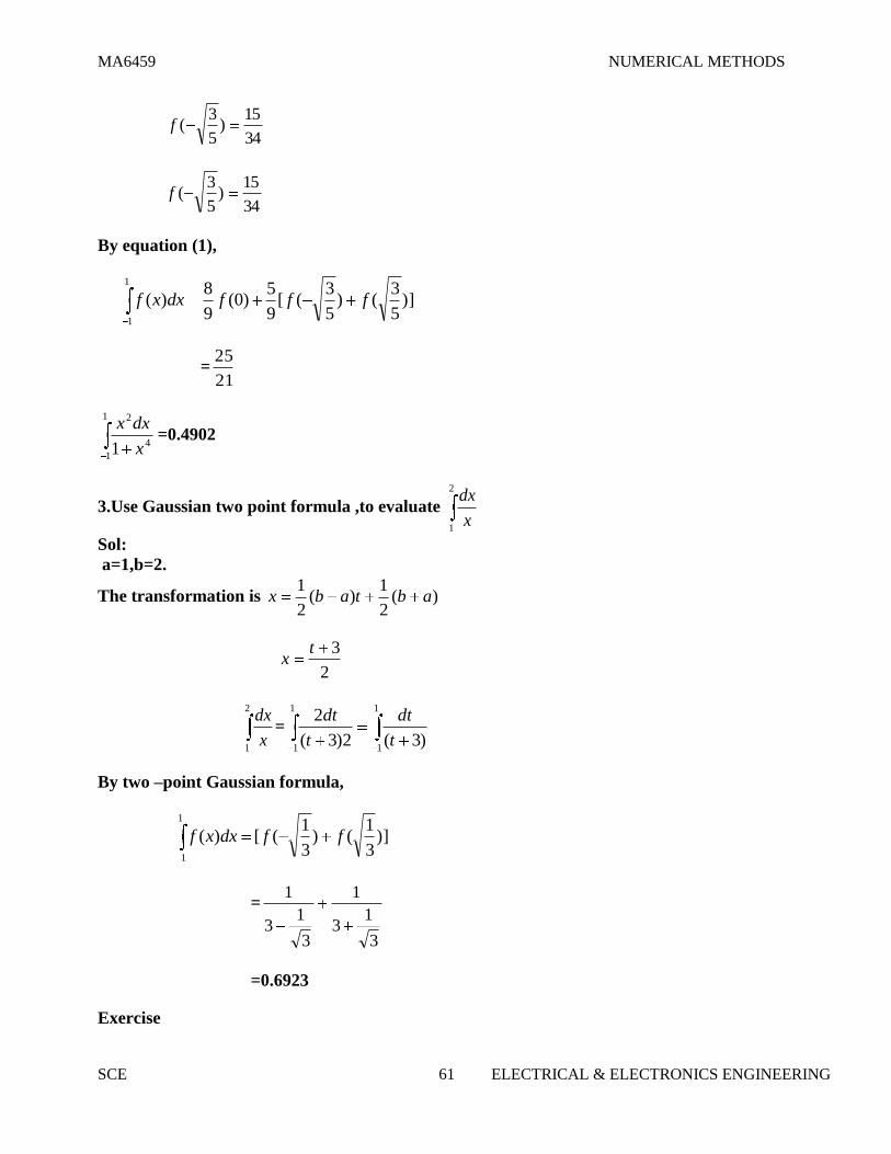
3.Use Gaussian two point formula ,to evaluate
2
1x
dx
Sol:
a=1,b=2.
The transformation is )(2
1)(
2
1abtabx
2
3tx
2
1x
dx=
1
1
1
1)3(2)3(
2
t
dt
t
dt
By two –point Gaussian formula,
)]3
1()
3
1([)(
1
1
ffdxxf
=
3
13
1
3
13
1
=0.6923
Exercise

MA6459 NUMERICAL METHODS
SCE 62 ELECTRICAL & ELECTRONICS ENGINEERING
1. Obtain two point and three point Gaussian formula for the gauss-chebyshev Quadrature
formula, given by
1
121
)(dx
x
xfI
Ans:2
3;
3101 x
2. Find
1
0
xdxI ,by Gaussian three point formula, correct to 4 decimal places.
Ans: 0.5
3. Evaluate
1
1
cosxdxI using Gaussian two point and three point formula
Ans: 1.6831
4. Evaluate
1
1
2 )1( dxxxI using Gaussian here point formula. Ans: 8/3
3.4 Double integrals
In this chapter we shall discuss the evaluation of
b
a
d
c
dxdyyxf ),( using
Trapezoidal and Simpson’s rule.
The formulae for the evaluation of a double integral can be obtained by repeatedly applying the
Trapezoidal and simpson’s rules.
Consider the integral m ny
y
x
x
dxdyyxfI
0 0
),( (1)
The integration in (1) can be obtained by successive application of any numerical integration
formula with respect to different variables.
Trapezoidal Rule for double integral
),(),(2),(
)],(),(2),([2
)],(),(2),([
4221202
211101
201000
yxfyxfyxf
yxfyxfyxf
yxfyxfyxfhk
I
Simpson’s rule for double integral
The general expression for Simpson’s rule for the double integral (1) can
also be derived.
In particular, Simpson’s rule for the evaluation of
),(),(4),(
)],(),(4),([4)],(),(4),([
9 11111
11110111
jijiji
jijjijijijiji
yxfyxfyxf
yxfyxfyxfyxfyxfyxfhkI
Problems:

MA6459 NUMERICAL METHODS
SCE 63 ELECTRICAL & ELECTRONICS ENGINEERING
1. Evaluate
1
0
1
0
dxdyeI yx using trapezoidal and Simpson’s rule
Sol:
Taking h=k=0.5
The table values of yxe are given a follows
(x0) (x1) (x2)
y\x 0 0.5 1
0 1 1.6487 2.7183
0.5 1.6487 2.7183 4.4817
1 2.7183 4.4817 7.3891
(i) Using Trapezoidal rule,we obtain
2
0
2
),(
y
y
x
x
dxdyyxfI where ),( yxf = yxe
),(),(2),(
)],(),(2),([2
)],(),(2),([
4221202
211101
201000
yxfyxfyxf
yxfyxfyxf
yxfyxfyxfhk
I
=3.0762
(ii) Using Simpson’s rule,we obtain
)],(),(4),(
)],(4),(16),(4)],(),(4),([
9 221202
211101201000
yxfyxfyxf
yxyxfyxfyxfyxfyxfhkI
=2.9543
2.Evaluate
1
0
1
01 yx
dxdyI by (i) Trapezoidal rule and (ii) Simpson’s rule with step sizes h=k=0.5
Sol:
Taking h=k=0.5
The table values of yx1
1are given a follows
(x0) (x1) (x2)
y\x 0 0.5 1
0 1 0.67 0.5
0.5 0.67 0.5 0.4
1 0.5 0.4 0.33

MA6459 NUMERICAL METHODS
SCE 64 ELECTRICAL & ELECTRONICS ENGINEERING
(i) Using Trapezoidal rule,we obtain
2
0
2
),(
y
y
x
x
dxdyyxfI where ),( yxf =yx1
1
),(),(2),(
)],(),(2),([2
)],(),(2),([
4221202
211101
201000
yxfyxfyxf
yxfyxfyxf
yxfyxfyxfhk
I
=0.5381
(i) Using Simpson’s rule,we obtain
)],(),(4),(
)],(4),(16),(4)],(),(4),([
9 221202
211101201000
yxfyxfyxf
yxyxfyxfyxfyxfyxfhkI
=0.5247
Exercise
1. Compute
1
0
1
0
xydxdyI with h=0.25 and k=0.5 using Simpson’s rule
Ans:I=0.25
2. Using Trapezoidal rule ,evaluate
2
1
2
1yx
dxdyI taking four sub intervlas
Ans:I=0.34065

MA6459 NUMERICAL METHODS
SCE 65 ELECTRICAL & ELECTRONICS ENGINEERING
Tutorial problems
Tutorial -1
1.Find the value of )3(f using divided differences, given data
x 0 1 4 5
F(x) 8 11 68 123
Ans:16
2.Find the first and second derivatives of the function at the point x=1.2 from the following data
X 1 2 3 4 5
Y 0 1 5 6 8
Ans:14.17
3.A rod is rotating in a plane .The angle θ (in radians) through which the rod has turned for various
values of time t (seconds) are given below
t 0 0.2 0.4 0.6 0.8 1.0 1.2
θ 0 0.122 0.493 1.123 2.022 3.220 4.666
Find the angular velocity and angular acceleration of the rod when t=06 seconds.
Ans:6.7275 radians/sec2.
4.From the table given below ,for what value of x, y is minimum? Also find this value of y.
X 3 4 5 6 7 8
Y 0.205 0.240 0.25 0.262 0.250 0.224
Ans:5.6875,0.2628
5.Find the first and second derivatives of y at x=500 from the following dat
x 500 510 520 530 540 550
y 6.2146 6.2344 6.2538 6.2792 6.2196 6.3099
Ans:0.002000,-0.0000040
Tutorial -2
1.Evaluate
1
01 x
xdx by Simpson’s 1/3 rule with h=0.1
2.Evalute
1
0
2cos xdx with h=0.1 by Simpson’s 1/3 rule.
3.Apply Trapezoidal and Simpson’s rules ,to find
1
0
21 dxx ,taking h=0.1.

MA6459 NUMERICAL METHODS
SCE 66 ELECTRICAL & ELECTRONICS ENGINEERING
4.Evaluate
6
01 x
dx by dividing the range into eight equal parts.
5.Using Simpson’s rule ,find 7log e approximately from the integral 7
1x
dxI
Tutorial -3
1.Evaluate
1
121 x
dx using Gaussian three point formula.
2.Evaluate
1
0
dxe x using three-term Gaussian Two-point Quadrature formula.
3.Evaluate 1
1
41 x
dx using Gaussian three point quadrature formula.
4. Evaluate1
1sin1
2cos
x
xdx using Gaussian two point quadrature formula.
5.Evaluate 4
2
2 )2( dxxx using Gaussian two point quadrature formula.
Question Bank
Part A
1. State the disadvantages of Taylor series method.
Sol:
In the differential equation = f(x,y) the function f(x,y) may have a complicated
algebraical structure. Then the evaluation of higher order derivatives may become tedious. This is
the demerit of this method.
2. Which is better Taylor’s method or R.K method?
Sol:
R.K methods do not require prior calculation of higher derivatives of y(x), as the Taylor
method does. Since the differential equations using in application are often complicated, the
calculation of derivatives may be difficult. Also R.K formulas involve the computations of
f(x,y) at various positions instead of derivatives and this function occurs in the given equation.
3. What is a predictor- collector method of solving a differential equation?
Sol:

MA6459 NUMERICAL METHODS
SCE 67 ELECTRICAL & ELECTRONICS ENGINEERING
predictor- collector methods are methods which require the values of y at xn, xn-1, xn-2,…
for computing the values of y at xn+1. We first use a formula to find the values of y at xn+1 and this
is known as a predictor formula. The value of y so get is improved or corrected by another formula
known as corrector formula.
4. Define a difference Quotient.
Sol:
A difference quotient is the quotient obtained by dividing the difference between two
values of a function, by the difference between the two corresponding values of the independent.
5. Write down the expression for nxatxdx
yd
dx
dy2
2
& by Newton’s backward difference formula.
6. State the formula for Simpson’s 3/8th
rule.
7. Write Newton’s forward derivative formula.
8.State the Romberg’s method integration formula fin the value of
b
a
dxxfI )( using h and h/2.
9.Write down the Simpson’s 3/8 rule of integration given (n+1) data.
10.Evaluate 4
1
)( dxxf from the table by Simpson’s 3/8 rule.
Part B
1.Apply three point Gaussian quadrature formula to evaluate .
2.Using Trapezoidal rule, evaluate numerically with h=0.2 along x-direction and
k=0.25 along y-direction.
3.Find the first and second derivative of the function tabulated below at x=0.6
x 0.4 0.5 0.6 0.7 0.8
y 1.5836 1.7974 2.0442 2.3275 2.6511
4. Using Romberg’s method to compute dx correct to 4 decimal places.Also evaluate
the same integral using three –point Gauss quadrature formula. Comment on the
obtained values by comparing with exact value of the integral which is equal to .
5.Evaluate using Simpson’s rule by taking h= and k = .
6.Find and at x=51 from the following data.
x 50 60 70 80 90
y 19.96 36.65 58.81 77.21 94.61

MA6459 NUMERICAL METHODS
SCE 68 ELECTRICAL & ELECTRONICS ENGINEERING
7.Evaluate I= by dividing the range into ten equal parts,using
(i)Trapezoidal rule
(ii)Simpson’s one-third rule. Verify your answer with actual integration.
8. Find the first two derivatives of at x=50 and x=56, for the given table :
x 50 51 52 53 54 55 56
Y=x1/3
3.6840 3.7084 3.7325 3.7325 3.7798 3.8030 3.8259
9.The velocities of a car running on a straight road at intervals of 2 minutes are given below:
Time(min) 0 2 4 6 8 10 12
Velocity(km/hr) 0 22 30 27 18 7 0
Using Simpson’s 1/3 rd
- rule find the distance covered by the car.
10. Given the following data, find y’(6) and the maximum value of y (if it exists)
x 0 2 3 4 7 9
Y 4 26 58 112 466 922

MA6459 NUMERICAL METHODS
SCE 69 ELECTRICAL & ELECTRONICS ENGINEERING
Chapter 4
Numerical Solution of ordinary Differential equations
Taylor’s series method
Introduction
An ordinary differential equation of order n is a relation of the form
0),......,,,( )(nyyyyxF where y=y(x) and r
rr
dx
ydy )(
.The solution of this differential equation
involves n constants and these constants are determined with help of n conditions.
Single step methods
In these methods we use information about the curve at one point and we do not
iterate the solution. The method involves more evaluation of the function. We will discuss the
Numerical solution by Taylor series method, Euler methods and Runge - Kutta methods all require
the information at a single point x=x0.
Multi step methods
These methods required fewer evaluations of the functions to estimate the solution
at a point and iteration are performed till sufficient accuracy is achieved. Estimation of error is
possible and the methods are called Predictor-corrector methods. In this type we mainly discuss
Milne’s and Adams-Bashforth method.
In the multi step method , to compute yn+1,we need the functional values yn,yn-1, yn-2 and yn-3.
4.1 Taylor Series method
Consider the first order differential equation 00 )(),,( yxyyxfdx
dy ……(1)
The solution of the above initial value problem is obtained in two types
Power series solution
Point wise solution
(i) Power series solution
+……. (2)

MA6459 NUMERICAL METHODS
SCE 70 ELECTRICAL & ELECTRONICS ENGINEERING
Where r
rr
dx
ydy
)(
0 at(
Using equation (1) the derivatives can be found by means of successive
differentiations .Expressions (2) gives the value for every value of x for which (2) converges.
(ii)Point wise solution
= +!1
h+ + +…
Where r
rr
mdx
ydy
)(at (
Where m=0,1,2,…….
Problems:
1. Using Taylor series method find y at x=0.1 if dx
dy= y-1,y(0)=1.
Solution:
Given = y-1 and =0, =1,h=.1
Taylor series formula for is
= +!1
h+ + +…
= y-1 = =0-1=-1
=2xy+ + =0+0=0
= + +2x
=2x +2y+ +2x
=2y+ 4x +
=2 +4 +
=2(1)+4(0)(-1)+( )(0)
=2
= +4 + +
= +4x +4 + + 2x
= + 6x +
= +6 +
=6(-1)+6(0)(0)+(0)(2)
=-6
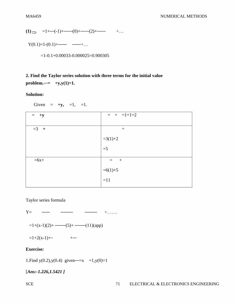
MA6459 NUMERICAL METHODS
SCE 71 ELECTRICAL & ELECTRONICS ENGINEERING
(1) =1+ (-1)+ (0)+ (2)+ +…
Y(0.1)=1-(0.1)+ +…
=1-0.1+0.00033-0.000025=0.900305
2. Find the Taylor series solution with three terms for the initial value
problem. = +y,y(1)=1.
Solution:
Given = +y, =1, =1.
= +y = + =1+1=2
=3 + +
=3(1)+2
=5
=6x+ = +
=6(1)+5
=11
Taylor series formula
Y= +…….
=1+(x-1)(2)+ (5)+ (11)(app)
=1+2(x-1)+ +
Exercise:
1.Find y(0.2),y(0.4) given =x +1,y(0)=1
[Ans:-1.226,1.5421 ]
MA6459 NUMERICAL METHODS
SCE 72 ELECTRICAL & ELECTRONICS ENGINEERING
2.Find y(0.1) given = y-1,y(0)=1
[Ans:- 0.9003 ]
EULER’S METHOD:
Introduction
In Taylor’s series method, we obtain approximate solutions of the initial value problem
00 )(),,( yxyyxfdx
dy as a power series in x , and the solution can be used to compare y
numerically specified value x near x0.
In Euler’s methods,we compute the values of y for .....2,1,0 iihxxi with a step h>0
i.e., )( ii xyy where .....2,1,0 iihxx
Euler’s method
= +f ),n=0,1,2,3,……
Modified Euler’s method
To compute for
(i) ),()1(
1 nnnn yxhfyy
(ii) ),(),([2
)1(
11 nnnnnn yhxfyxfh
yy error n=0,1,2…..
Error=O(h3)
Note
In Euler method yyy nn 1
Where ),( 00 yxhfy
Where slopeyxf ),( 00 at
),( 00 yxf .
In modified Euler’s method yyy nn 1 ,
Where y =h[average of the slopes at x0 and x1](Or)

MA6459 NUMERICAL METHODS
SCE 73 ELECTRICAL & ELECTRONICS ENGINEERING
=h[average of the values of dx
dy at the ends of the interval 0x to
1x ]
1.Using Euler’s method compute y in the range 0 .5 if y satisfies 3x+ ,y(0)=1.
Solution:
Here f(x,y) = 3x+ , =0, =1
By Euler’s method
= +f ),n=0,1,2,3,…… (1)
Choosing h=0.1, we compute the value of y using (1)
= +f ),n=0,1,2,3,……
= +hf( )=1+(0.1)[3(0)+ ] =1.1
= +hf( )=1.1+(0.1)[0.3+ ] =1.251
= +hf( )=1.251+(0.1)[0.6+ ] =1.4675
= +hf( )=1.4675+(0.1)[0.9+ ] =1.7728
= +hf( )=1.7728+(0.1)[1.2+ ] =2.2071
Exercise:
1.Given that yxdx
dyand y=1 when x=0,Find y when x=0.05,0.10 and 0.15 using modified
Euler method.
Ans:
1.0525,1.1103,1.1736
2.Using Euler’s method,solve .1)0(, yxyyxy Compute y(1.0) with h= 0.2
Ans:3.9778
MODIFIED EULER’S METHOD:
1. Given =-x , y(0)=2. Using Euler’s modified method, find y(0.2)in two steps of 0.1 each.
Solution:
Let = +h. here , and h=0.1

MA6459 NUMERICAL METHODS
SCE 74 ELECTRICAL & ELECTRONICS ENGINEERING
The value of y at x= is
By modified Euler method,
= hf(
f( f( ]
Here f(x,y) = -x
f( = - =0
2+(0.1)(0)=2
2+ [f(0,2)+f(0.1,2)]
=2+0.05[0+(-0.1)(4)]
1.98
Y(0.1)=1.98
To find y(0.2)
=1.98 –(0.1)(0.1)(1.98)=1.9602
+ f( f( ]
=1.9602-(0.05)[(0.198)+(0.39204)]
Hence y(0.2)=1.9307
Runge-kutta method
The Taylor’s series method of solving differential equations numerically is restricted
because of the evaluation of the higher order derivatives.Runge-kutta methods of solving intial
value problems do not require the calculations of higher order derivatives and give greater

MA6459 NUMERICAL METHODS
SCE 75 ELECTRICAL & ELECTRONICS ENGINEERING
accuracy.The Runge-Kutta formula posses the advantage of requiring only the function values at
some selected points.These methods agree with Taylor series solutions upto the term in hr where r
is called the order of that method.
Fourth-order Runge-Kutta method
This only is commonly used for solving initial values problem
00 )(),,( yxyyxfdx
dy
Working rule
The value of )( 11 xyy where hxx 01 where h is the step-size is obtained as follows.We
calculate successively.
),(
)2
,2
(
)2
,2
(
),(
34
23
12
1
kyhxhfk
ky
hxhfk
ky
hxhfk
yxhfk
mm
mm
mm
mm
Finally compute the increment
]22[6
143211 kkkkyy mm where m=0,1,2……
Problems
1. Obtain the value of y at x =0.2 if satisfies 1,0, 00
2 yxxyxdx
dy using Runge-kutta
method of fourth order.
Sol:
Here 1,0,),( 00
2 yxxyxyxf
Let hxx 01
Choosing h=0.1,x1=0.1
Then by R-K fourth order method,

MA6459 NUMERICAL METHODS
SCE 76 ELECTRICAL & ELECTRONICS ENGINEERING
]22[6
1432101 kkkkyy
0110050.0),(
00525.0)2
,2
(
00525.0)2
,2
(
0),(
3004
2003
1002
001
kyhxhfk
ky
hxhfk
ky
hxhfk
yxhfk
y(0.1)=1.0053
To find )( 22 xyy where hxx 12 Taking x2=0.2
]22[6
1432112 kkkkyy
02409.0),(
01728.0)2
,2
(
01727.0)2
,2
(
0110.0),(
3114
2113
1112
111
kyhxhfk
ky
hxhfk
ky
hxhfk
yxhfk
y(0.2)=1.0227
2.Apply Runge –kutta method to find an approximate value of y for x=0.2 in steps of 0.1 if
1)0(,2 yyxdx
dy,correct to four decimal places.
Sol:
Here f(x,y)=x+y2,x0=0,y(0)=1
Then by R-K fourth order method,
]22[6
1432101 kkkkyy

MA6459 NUMERICAL METHODS
SCE 77 ELECTRICAL & ELECTRONICS ENGINEERING
1347.0),(
1168.0)2
,2
(
1152.0)2
,2
(
1.0),(
3004
2003
1002
001
kyhxhfk
ky
hxhfk
ky
hxhfk
yxhfk
y(0.1)=1.1165
To find )( 22 xyy
where hxx 12 Taking x2=0.2
]22[6
1432112 kkkkyy
1823.0),(
1576.0)2
,2
(
1151.0)2
,2
(
1347.0),(
3114
2113
1112
111
kyhxhfk
ky
hxhfk
ky
hxhfk
yxhfk
y(0.2)=1.2736
Exercise:
1.Use Runge-kutta method to find when x=1.2 in steps of 0.1 ,given that 5.1)1(,22 yyxdx
dy
Ans:1.8955, 2.5043
2.Solve 1xyy for x=0.2(0.2)0.6 by Fourht order method,given that y=2 when x=0
Ans: 2.2431,2.5886, 3.0719

MA6459 NUMERICAL METHODS
SCE 78 ELECTRICAL & ELECTRONICS ENGINEERING
Multi step methods(Predictor-Corrector Methods)
Introduction
Predictor-Corrector Methods are methods which require function values at
321 ,,, nnnn xxxx for the compulation of the function value at xn+1.A predictor is used to find the
value of y at xn+1 and then a corrector formula to improve the value of yn+1.
The following two methods are discussed in this chapter.
Milne’s method
Adam’s method.
Milne’s Predictor-Corrector method
Milne’s predictor formula is
And the error = )(45
14 )(5
vyh
Where 13 nn xx
Milne’s corrector formula is
And the error = )(90
)(5
vyh
Where 11 nn xx

MA6459 NUMERICAL METHODS
SCE 79 ELECTRICAL & ELECTRONICS ENGINEERING
Problems
1.Using Milne’s method ,compute y(0.8) given that
6841.0)6.0(,4228.0)4.0(,2027.0)2.0(,1)0(,1 2 yyyyydx
dy
Sol:
We have the following table of values
X
y
Y’=
1+y2
0
0.2
0.4
0.6
0
0.2027
0.4228
0.6841
1.0
1.0411
1.1787
1.4681
4681.1,1787.1,0411.1,1
6841.0,4228.0,2027.0,0
6.0,4.0,2.0,0
3210
3210
3210
yyyy
yyyy
xxxx
To find y(0.8)
8.08x ,here h=0.2
Milne’s predictor formula is
where ).
=1.0239
=2.0480
Milne’s corrector formula is
where ).
=1.0294
y(0.8)=1.0294
2. Compute y(0.4) by Milne’s method ,given that 1)0(, yyxy with h=0.1 use Taylor’s
method to find the starting values.

MA6459 NUMERICAL METHODS
SCE 80 ELECTRICAL & ELECTRONICS ENGINEERING
Ans:1.9816, 1.5774
Adams-bashforth Predictor and Adams-bashforth corrector formula.
Adams-bash forth predictor formula is
Adams –bash forth corrector formula is
where ).
The error in these formulas are )(720
251 5 ivfh and )(720
19 5 ivfh
Problems
1.Given 7379.1)6.0(,4682.1)4.0(,2186.1)2.0(,1)0(,2 yyyyxyy estimate y(0.8) by
Adam’s-Bashforth method.
Sol:
3779.1,3082.1,1782.1,1
7379.1,4682.1,2186.1,0
6.0,4.0,2.0,0
3210
3210
3210
yyyy
yyyy
xxxx
To find 4y for 8.04x here h=0.2
By Predictor formula,
=2.0146
3746.14y

MA6459 NUMERICAL METHODS
SCE 81 ELECTRICAL & ELECTRONICS ENGINEERING
=2.0145
y(0.8)=2.0145
2.Given 6841.0)6.0(,4228.1)4.0(,2027.0)2.0(,0)0(,1 2 yyyyyy ,Estimate y(0.8)
using Adam’s method.
Sol:
4680.1,1786.1,0411.1,1
6841.0,4228.0,2027.0,0
6.0,4.0,2.0,0
3210
3210
3210
yyyy
yyyy
xxxx
To find 4y for 8.04x here h=0.2
By Predictor formula,
=1.0235
0475.24y
=1.0297
y(0.8)=1.0297
MA6459 NUMERICAL METHODS
SCE 82 ELECTRICAL & ELECTRONICS ENGINEERING
Tutorial problems
Tutorial-1
1.Using Taylor\s series method ,find y(0.2) approximately ,given that xey
dx
dy32 y(0)=0
correct to four decimal places.
2.Compute y for x=0.1,0.2 correct to four decimal places given 2)0(, yxydx
dyusing taylor’s
series method.
3.Using Euler’s Modified method ,find the values of y at x=0.1,0.2,0.3,0.4 given
0)0(,1 yydx
dy correct to four decimal places.
4. Using Euler’s method ,find y(0.1),y(0.2) and y(0.3)given that 0)0(,1 2 yydx
dy
5.Using Euler’s modified method, find a solution of the equation yxdx
dy with the initial
condition y(0)=1 for the range 6.00 x in steps of 0.2.
Tutorial-2
1.Use R-K fourth order method, of find y at x=0.1(0.1)0.3 if 1)0(,1 2x
xyy
2.Apply R-K method of order 4 to solve 1)1(,31 yxydx
dywith h=0.1
3.Using R-K method to solve 0)0(,1)0(,2
2
2
yyydx
dyx
dx
ydto find y(0.2) and )2.0(y
4.Use the R-K method of fourth order ,find y(0.1)=1 given that
0)0(,1)0(,122
2
2
yyxydx
dyx
dx
yd
5.Compute y and z for x=0.1 given 1)0(,0)0(,;1 zyyxdx
dzz
dx
dy

MA6459 NUMERICAL METHODS
SCE 83 ELECTRICAL & ELECTRONICS ENGINEERING
Tutorial-3
1.Apply Milne’s method ,to find y(0.4) given that .1)0(,2 yyxyy Use Taylor’s series
method to compute y(0.1),y(0.2),y(0.3).
2.using Adam-Bashforth method, find the solution of yxdx
dy at x=0.4,given the values
y(0)=1,,y(0.1)=1.1103,y(0.2)=1.2428,y(0.3)=1.3997
3.Using adam’s method ,determine y(0.4) given that
0228.1)3.0(,0101.1)2.0(,0025.1)1.0(,1)0(,2
1yyyyxy
dx
dy
4.Given )3.0(),2.0(),1.0(,1)0(,22
1yycomputeyyyxy by the fourth order R-K method and
y(0.4) by Adam’s method.
5.Compute y for x=0.1(0.1)0.3 by the fourth order R-K method and y(0.4) by Adam’s method ,if
1)0(,41 yyxdx
dy

MA6459 NUMERICAL METHODS
SCE 84 ELECTRICAL & ELECTRONICS ENGINEERING
Question Bank
Part A
1.State Modified Euler algorithm to solve y’= ,y(x0)=y) at x=x0 +h
Sol:
2. State the disadvantage of Taylor series method.
Sol:
In the differential equation f (x, y), = f (x, y), the function f (x, y),may have a
complicated algebraical structure. Then the evaluation of higher order derivatives may
become tedious. This is the demerit of this method.
3. Write the merits and demerits of the Taylor method of solution.
Sol:
The method gives a straight forward adaptation of classic to develop the solution
as an infinite series. It is a powerful single step method if we are able to find the
successive derivatives easily. If f (x.y) involves some complicated algebraic structures
then the calculation of higher derivatives becomes tedious and the method fails.This is
the major drawback of this method. However the method will be very useful for finding
the starting values for powerful methods like Runge - Kutta method, Milne’s method etc.
4.Which is better Taylor’s method or R. K. Method?(or) State the special advantage of
Runge-Kutta method over taylor series method
Sol:
R.K Methods do not require prior calculation of higher derivatives of y(x) ,as the
Taylor method does. Since the differential equations using in applications are often
complicated, the calculation of derivatives may be difficult.
Also the R.K formulas involve the computation of f (x, y) at various positions, instead
of derivatives and this function occurs in the given equation.
5.Compare Runge-Kutta methods and predictor – corrector methods for solution of
initial value problem.
Sol:Runge-Kutta methods
1.Runge-methods are self starting,since they do not use information from previously
calculated points.

MA6459 NUMERICAL METHODS
SCE 85 ELECTRICAL & ELECTRONICS ENGINEERING
2.As mesne are self starting,an easy change in the step size can be made at any stage.
3.Since these methods require several evaluations of the function f (x, y), they are time
consuming.
4.In these methods,it is not possible to get any information about truncation error.
Predictor Corrector methods:
1.These methods require information about prior points and so they are not self starting.
2.In these methods it is not possible to get easily a good estimate of the truncation error.
6. What is a Predictor-collector method of solving a differential equation?
Sol:
Predictor-collector methods are methods which require the values of y at xn,xn-1,xn-2,…
for computing the value of y at . x n+1 We first use a formula to find the
value of y at . x n+1 and this is known as a predictor formula.The value of y so got is
improved or corrected by another formula known as corrector formula.
7. State the third order R.K method algorithm to find the numerical solution of the
first order differential equation.
Sol:
To solve the differential equation y′ = f (x, y) by the third order R.K method, we use
the following algorithm.
and
8.Write Milne’s predictor formula and Milne’s corrector formula.
Sol:
Milne’s predictor formula is
where ).
Milne’s corrector formula is
where ).
9.Write down Adams-bashforth Predictor and Adams-bashforth corrector formula.
Sol:
Adams-bashforth predictor formula is
Adams –bashforth corrector formula is
where ).
10.By Taylor’s series method ,find y(1.1) given 1)1(, yyxy
Ans:1.2053

MA6459 NUMERICAL METHODS
SCE 86 ELECTRICAL & ELECTRONICS ENGINEERING
Part B
1.Using Runge-Kutta method find an approximate value of y for x=0.20 if =x + given
that y=1 when x=0.
2.Given that y” +xy’+y =0,y(0)=1,y’(0)=0 obtain y for x=0,1,0.2,0.3 by Taylor’s series method
and find the solution for y(0.4) by Milne’s method.
3.Obtain y by Taylor series method,given that y’=xy+1,y(0)=1for x=0.1 and 0.2 correct to
four decimal places.4.Solve for y(0.1) and z(0.1) from the simultaneous differential equations
=2y +z: =y-3z; y(0)=0,z(0)=0.5 using Runge-Kutta method of the fourth order.
5.Using Adams method find y(1.4) given y’=x2(1+y) , y(1)=1, y(1.1)=1.233, y(1.2)=1.548 and
y(1.3)=1.979.
6.Using Milne’s Predictor-Corrector formula to find y(0.4) given = ,
y(0)=1,y(0.1)=1.06, y(0.2)=1.12 and y(0.3)=1.21.
7.Using Modified Euler’s method , find y(4.1) and y(4.2) if 5x + -2 =0: y(4)=1.
8.Given that =1+ ; y(0.6)=0.6841, y(0.4)=0.4228, y(0.2)=0.2027, y(0)=0, find y(-0.2) using
Milne’s method.
9.Given that y’=y-x2 ; y(0)=1: y(0.2)=1.1218; y(0.4)=1.4682 and y(0.6)= 1.7379 , evaluate
y(0.8) by Adam’s predictor –Corrector method.10.Solve by Euler’s method the following
differential equation x=0.1, correct to four decimal places, = with initial condition
y(0)=1.

MA6459 NUMERICAL METHODS
SCE 87 ELECTRICAL & ELECTRONICS ENGINEERING
Chapter 5
Boundary value Problems in ODE&PDE
5.1 Solution of Boundary value problems in ODE
Introduction
The solution of a differential equation of second order of the form
0),,,( yyyxF contains two arbitrary constants. These constants are determined by means of
two conditions. The conditions on y and y or their combination are prescribed at two different
values of x are called boundary conditions.
The differential equation together with the boundary conditions is called a
boundary value problem.
In this chapter ,we consider the finite difference method of solving linear boundary value problems
of the form.
Finite difference approximations to derivatives
First derivative approximations
)()()(
)( hOh
xyhxyxy (Forward difference)
)()()(
)( hOh
hxyxyxy (Backward difference)
)(2
)()()( 2hO
h
xhyhxyxy (Central difference)
Second derivative approximations
)()()(2)(
)( 2
2hO
h
hxyxyhxyxy (Central difference)
Third derivative approximations
]22[2
1)( 21123 iiii
iii yyyyh
xy
Fourth derivative approximations

MA6459 NUMERICAL METHODS
SCE 88 ELECTRICAL & ELECTRONICS ENGINEERING
]464[1
)( 21124 iiiii
iv yyyyyh
xy
Solution of ordinary differential equations of Second order
h
yyy ii
i2
11
2
11 2
h
yyyy iii
i
Problems
1. Solve 2)2(,1)1(,0 yyyyx with h=0. And h=0.25 by using finite difference method.
Sol:
(i) Divide the interval[1,2] into two sub-intervals with h=(2-1)/2=0.5
X0=1 x1=1.5 x2=2
Let hxx ii 1 ,
Here 2,5.1,1 210 xxx
By Boundary conditions are 2)2(,1)1( yy
2,1 20 yy
We have to determine 1y for 1x =1.5
Replacing the derivative y by 2
11 2
h
yyyy iii
0]2[ 112 iiiii yyyy
h
x (1)
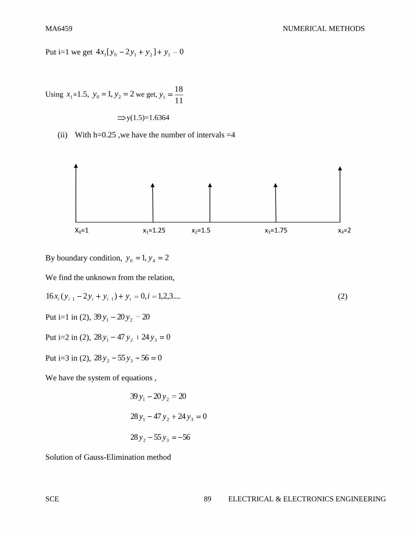
MA6459 NUMERICAL METHODS
SCE 89 ELECTRICAL & ELECTRONICS ENGINEERING
Put i=1 we get 0]2[4 12101 yyyyx
Using 1x =1.5, 2,1 20 yy we get,11
181y
y(1.5)=1.6364
(ii) With h=0.25 ,we have the number of intervals =4
X0=1 x1=1.25 x2=1.5 x3=1.75 x4=2
By boundary condition, 2,1 40 yy
We find the unknown from the relation,
....3,2,1,0)2(16 11 iyyyyx iiiii (2)
Put i=1 in (2), 202039 21 yy
Put i=2 in (2), 0244728 321 yyy
Put i=3 in (2), 0565528 32 yy
We have the system of equations ,
202039 21 yy
0244728 321 yyy
565528 32 yy
Solution of Gauss-Elimination method

MA6459 NUMERICAL METHODS
SCE 90 ELECTRICAL & ELECTRONICS ENGINEERING
=
The equivalent system is
403.3838.1
513.0445.1
513.0513.0
3
32
21
y
yy
yy
By back substitution, the solution is 851.13y , 635.12y , 351.11y
Hence y(1.25)=1.351,y(1.5)=1.635,y(1.75)=1.851
Exercise
1. Solve by finite difference method, the boundary value problem 02
2
ydx
ydwith y (0) =0
and y (2) =4.
Ans: 3583.23y , 3061.12y , 5805.01y
2. Solve 1)2(0)1(,0 andyyyyx with h=0.5
5.2 Solution of Laplace Equation and Poisson equation
Partial differential equations with boundary conditions can be solved in a
region by replacing the partial derivative by their finite difference approximations. The finite
difference approximations to partial derivatives at a point (xi,yi) are given below. The xy-plane is
divided into a network of rectangle of lengh hx and breadth ky by drawing the lines x=ih
and y=jk, parallel to x and y axes.The points of intersection of these lines are called grid points or

MA6459 NUMERICAL METHODS
SCE 91 ELECTRICAL & ELECTRONICS ENGINEERING
mesh points or lattics points.The grid points ),( ji yx is denoted by (i,j) and is surrounded by the
neighbouring grid points (i-1,j),(i+1,j),(i,j-1),(i,j+1) etc.,
Note
The most general linear P.D.E of second order can be written as
),(2
22
2
2
yxfFuy
uE
x
uD
y
uC
yx
uB
x
uA (1)
Where A,B,C,D,E,F are in general functions of x and y.
The equation (1) is said to be
Elliptic if B2-4AC<0
Parabolic if B2-4AC=0
Hyperbolic if B2-4AC>0
Solution of Laplace equation uxx+uyy=0
][4
11,1,,1,1, jijijijiji uuuuu
This formula is called Standard five point formula
][4
11,11,11,11,1, jijijijiji uuuuu
This expression is called diagonal five point formula.
Leibmann’s Iteration Process
We compute the initial values of 921 ,....., uuu by using standard five point formula and
diagonal five point formula .First we compute 5u by standard five point formula (SFPF).
][4
13111575 bbbbu
We compute 9731 .,, uuuu by using diagonal five point formula (DFPF)
][4
1153511 bbubu
][4
173553 bbbuu

MA6459 NUMERICAL METHODS
SCE 92 ELECTRICAL & ELECTRONICS ENGINEERING
][4
111155137 bbubu
][4
1591179 ubbbu
Finally we compute 8642 ,,, uuuu by using standard five point formula.
][4
131352 uubuu
][4
1715514 ubuuu
][4
175936 buuuu
][4
1591178 uubuu
The use of Gauss-seidel iteration method to solve the system of equations obtained by finite
difference method is called Leibmann’s method.
Problems
1.Solve the equation 02u for the following mesh,with boundary vaues as shown using
Leibmann’s iteration process.
1u 2u 3u
4u 5u 6u
7u 8u 9u
0 500 1000 500 0
Sol:
Let 1u , 2u …… 9u be the values of u at the interior mesh points of the given region.By symmetry about
the lines AB and the line CD,we observe
31 uu 1u = 7u
2u 8u 4u 6u

MA6459 NUMERICAL METHODS
SCE 93 ELECTRICAL & ELECTRONICS ENGINEERING
3u 9u 7u 9u
1u = 3u 7u = 9u , 2u 8u , 4u 6u
Hence it is enough to find ,1u 2u , ,4u 5u
Calculation of rough values
5u =1500
1u =1125
2u =1187.5
4u =1437.5
Gauss-seidel scheme
]1500[4
1421 uuu
]10002[4
1512 uuu
]2000[4
1454 uuu
]22[4
1425 uuu
The iteration values are tabulated as follows
Iteration
No k
1u
2u
4u
5u
0
1
2
3
4
5
6
7
8
9
10
11
12
1500
1031.25
1000
968.75
953.1
945.3
941.4
939.4
938.4
937.9
937.7
937.6
937.6
1125
1125
1062.5
1031.25
1015.3
1007.8
1003.9
1001.9
1000.9
1000.4
1000.2
1000.1
1000.1
1187.5
1375
1312.5
1281.25
1265.6
1257.8
1253.9
1251.9
1250.9
1250.4
1250.2
1250.1
1250.1
1437.5
1250
1187.5
1156.25
1140.6
1132.8
1128.9
1126.9
1125.9
1125.4
1125.2
1125.1
1125.1
1u = 3u 7u = 9u =937.6, 2u 8u =1000.1, 4u 6u =1250.1, 1.11255u

MA6459 NUMERICAL METHODS
SCE 94 ELECTRICAL & ELECTRONICS ENGINEERING
2.When steady state condition prevail,the temperature distribution of the plate is represented by
Laplace equation uxx+uyy=0.The temperature along the edges of the square plate of side 4 are given
by along x=y=0,u=x3 along y=4 and u=16y along x=4,divide the square plate into 16 square
meshes of side h=1 ,compute the temperature at all of the 9 interior grid points by Leibmann’s
iteration process.
Solution of Poisson equation
An equation of the type ),(2 yxfu i.e., is called ),(2
2
2
2
yxfy
u
x
upoisson’s equation
where f(x,y) is a function of x and y.
),(4 2
,1,,1,1 jhihfhuuuu jijijiji
This expression is called the replacement formula.applying this equation at each internal mesh
point ,we get a system of linear equations in ui,where ui are the values of u at the internal mesh
points.Solving the equations,the values ui are known.
Problems
1.Solve the poisson equation )10(10 222 yxu over the square mesh with sides
x=0,y=0,x=3,y=3 and u=0 on the boundary .assume mesh length h=1 unit.
Sol: 0 0
0 A u1 u2 B J=3
0 J=2
0 u3 u4 J=1
0 C D
I=0 i=1 i=2 i=3 x
Here the mesh length 1hx
Replacement formula at the mesh point (i,j)
)10(104 22
,1,1,,1,1 jiuuuuu jijijijiji (1)

MA6459 NUMERICAL METHODS
SCE 95 ELECTRICAL & ELECTRONICS ENGINEERING
5.67,5.82,75
1504
1204
1504
3241
432
341
132
uuuu
uuu
uuu
uuu
2.Solve the poisson equation 10;10,812
2
2
2
yxxyy
u
x
uand
u(0,y)=u(x,0)=0,u(x,1)=u(1,y)=100 with the square meshes ,each of length h=1/3.
5.3 Solution of One dimensional heat equation
In this chapter, we will discuss the finite difference solution of one dimensional heat flow
equation by Explicit and implicit method
Explicit Method(Bender-Schmidt method
Consider the one dimensional heat equation 2
22
x
u
t
u.This equation is an example of
parabolic equation.
jijijiji uuuu ,1,,11, 21 (1)
Where 2ah
k
Expression (1) is called the explicit formula and it valid for 2
10
If λ=1/2 then (1) is reduced into
][2
1,1,11, jijiji uuu
(2)
This formula is called Bender-Schmidt formula.
Implicit method (Crank-Nicholson method)
jijijijijiji uuuuuu ,1,,11,11,1,1 )1(2)1(2
This expression is called Crank-Nicholson’s implicit scheme. We note that Crank Nicholson’s
scheme converges for all values of λ
When λ=1, i.e., k=ah2 the simplest form of the formula is given by
][4
1,1,11,11,11, jijijijiji uuuuu
The use of the above simplest scheme is given below.

MA6459 NUMERICAL METHODS
SCE 96 ELECTRICAL & ELECTRONICS ENGINEERING
The value of u at A=Average of the values of u at B, C, D, E
Note
In this scheme, the values of u at a time step are obtained by solving a system of linear equations
in the unknowns ui.
Solved Examples
1.Solve txx uu 2 when u(0,t)=0,u(4,t)=0 and with initial condition u(x,0)=x(4-x) upto t=sec
assuming 1hx
Sol:
By Bender-Schmidt recurrence relation ,
][
2
1,1,11, jijiji uuu
(1)
For applying eqn(1) ,we choose 2
2ahk
Here a=2,h=1.Then k=1
By initial conditions, u(x,0)=x(4-x) ,we have
3,4,3,
3,2,1)4(
0,30,20,1
0,
uuu
iiiui
By boundary conditions, u(0,t)=0,u0=0,u(4,0)=0 ju j 0,4

MA6459 NUMERICAL METHODS
SCE 97 ELECTRICAL & ELECTRONICS ENGINEERING
Values of u at t=1
2][2
1
3][2
1
2][2
1
][2
1
0,40,21,3
0,30,11,2
0,20,01,1
0,10,11,
uuu
uuu
uuu
uuu iii
The values of u up to t=5 are tabulated below.
j\i
0
1
2
3
4
0
1
2
3
4
5
0
0
0
0
0
0
3
2
1.5
1
0.75
0
4
3
2
1.5
1
0.75
3
2
1.5
1
0.75
0.5
0
0
0
0
0
0
2.Solve the equation 2
2
x
u
t
u
subject to the conditions u(0,t)=u(5,t)=0 and
)25()0,( 22 xxxutaking h=1 and k=1/2,tabulate the values of u upto t=4 sec.
Sol:
Here a=1,h=1
For λ=1/2,we must choose k=ah2/2

MA6459 NUMERICAL METHODS
SCE 98 ELECTRICAL & ELECTRONICS ENGINEERING
K=1/2
By boundary conditions
0,144,144,84,24
5,4,3,2,1,0),25(
)25()0,(
00),5(
00),0(
0,50,40,30,20,1
22
0,
22
,5
,0
uuuuu
iiiu
xxxu
jutu
jutu
i
j
j
By Bender-schmidt realtion,
][2
1,1,11, jijiji uuu
The values of u upto 4 sec are tabulated as follows
j\i
0
1
2
3
4
5
0
0.5
1
1.5
2
2.5
3
3.5
4
0
0
0
0
0
0
0
0
0
24
42
42
39
30
26.625
19.875
17.5312
13.0312
84
84
78
60
53.25
39.75
35.0625
26.0625
22.9687
144
144
78
67.5
49.5
43.5
32.25
28.4062
21.0938
144
72
57
39
33.75
24.75
21.75
16.125
14.2031
0
0
0
0
0
0
0
0
0

MA6459 NUMERICAL METHODS
SCE 99 ELECTRICAL & ELECTRONICS ENGINEERING
5.4 Solution of One dimensional wave equation
Introduction
The one dimensional wave equation is of hyperbolic type. In this chapter, we discuss the
finite difference solution of the one dimensional wave equation xxtt uau 2.
Explicit method to solve xxtt uau 2
1,,1,1
22
,
22
1, )1(2 jijijijiji uuuauau (1)
Where =k/h
Formula (1) is the explicit scheme for solving the wave equation.
Problems
1.Solve numerically , ttxx uu4 with the boundary conditions u(0,t)=0,u(4,t)=0 and the initial
conditions ),4()0,(&0)0,( xxxuxut taking h=1.Compute u upto t=3sec.
Sol:
Here a2=4
A=2 and h=1
We choose k=h/a k=1/2
The finite difference scheme is
2,3
22/04
0,3,3,0
4,3,2,1,0),4()4()0,(
00),4(&0),0(
1,31,2
1,1
0,40,20,10,0
0,
,4,0
1,,1,11,
uu
u
uuuu
iiiuxxxu
jutuutu
uuuu
i
jj
jijijiji
The values of u for steps t=1,1.5,2,2.5,3 are calculated using (1) and tabulated below.
j\i 0 1 2 3 4
0 0 3 4 3 0
1 0 2 3 2 0
2 0 0 0 0 0
3 0 -2 3 -2 0
4 0 -3 -4 3 0
5 0 -2 -3 -2 0
6 0 0 0 0 0

MA6459 NUMERICAL METHODS
SCE 100 ELECTRICAL & ELECTRONICS ENGINEERING
2.Solve ttxx uu given u(0,t)=0,u(4,t)=0,u(x,0)= .0)0,(&2
)4()0,( xu
xxxu t Take h=1.Find
the solution upto 5 steps in t-direction.
Sol:
Here a2=4
A=2 and h=1
We choose k=h/a k=1/2
The finite difference scheme is
1,5.1
1
0,5.1,2,5.1,0
4,3,2,1,0,2/)4(2/)4()0,(
00),4(&0),0(
1,31,2
1,1
0,40,30,20,10,0
0,
,4,0
1,,1,11,
uu
u
uuuuu
iiiuxxxu
jutuutu
uuuu
i
jj
jijijiji
The values of u upto t=5 are tabulated below.
j\i 0 1 2 3 4
0 0 1.5 2 1.5 0
1 0 1 1.5 1 0
2 0 0 0 0 0
3 0 -1 -1.5 -1 0
4 0 -1.5 -2 -1.5 0
5 0 -1 -1.5 -1 0
Exercise
1.Solve 2
2
2
2
x
u
t
u,0<x<1,t>0 given that u(x,0)=100sinπx, 0),1(),0(,0)0,( tutux
t
u
Taking h=1/4 compute u for 4 time steps.
2. Solve 2
2
2
2
x
u
t
u,0<x<1,t>0 given that u(x,0)=100(x-x
2), 0),1(),0(,0)0,( tutux
t
u
compute u for 4 time steps taking h=0.25.

MA6459 NUMERICAL METHODS
SCE 101 ELECTRICAL & ELECTRONICS ENGINEERING
Tutorial problems
Tutorial-1
1.Solve the boundary value problem 01064yy with y(0)=y(1)=0 by the finite difference
method.
Ans:0.129,0.147
2.Determine the values of y at the pivotal pointa of the interval (0,1) if y satisfies the boundary
value problem 0)1()0()1()0(,8181 2 yyyyxyy ivtake n=3.
Ans:0.1222,0.1556
3.Write down the finite difference analogue of the equation 0yyxx uu solve it for the region
bounded by the squre 40,40 yx and the boundary conditions being given as,u=0 at
x=0;u=8+2y at x=4 ; 2/2xu at y=0; 2xu at y=4.with h=k=1,use Gauss-seidel method to
compute the values at the initial at the internal mesh points.
Ans:2,4.9,9,2.1,4.7,8.1,1.6,3.7,6.6
4.Solve the poisson equation 10;10,81 yxxyuu yyxx and
u(0,y)=u(x,0)=0,u(x,1)=u(1,y)=100 with the square meshs,each of length h=1/3
Ans:51.08,76.54,25.79
5.Solve by Crank- Nicholson’s implicit method, 0,10, txuu xxt with
.0),1(,0),0(),(100)0,( 2 tutuxxxu compute u for one time step with h=0.25.
Ans:9.82,14.29
Tutorial -2
1.Solve the boundary value problem 01064yy with y(0)=y(1)=0by the finite difference
method.
Ans: y(0.5)=0.147,y(0.25)=y(0.75)=0.129
2.Solve 1)2(,0)1(,0 yyyyx with h=0.5
Ans: y (0)=1.6552 and y(0.5)=1.4483
3.When steady condition prevail,the temperature distribution of the plate is representd by Laplce
equation 0yyxx uu .The temperature along the edges of the square plate of side 4 are given by
u=0 along x=y=0;u=x3 along y=4 and u=16y alon x=4.Divide the square plate into 16 square
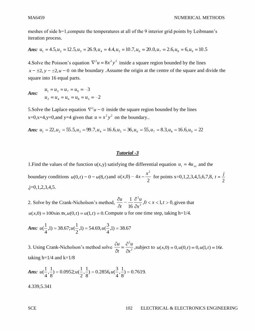
MA6459 NUMERICAL METHODS
SCE 102 ELECTRICAL & ELECTRONICS ENGINEERING
meshes of side h=1,compute the temperatures at all of the 9 interior grid points by Leibmann’s
iteration process.
Ans: 5.10,6,6.2,0.20,7.10,4.4,9.26,5.12,5.4 987654321 uuuuuuuuu
4.Solve the Poisson’s equation 222 8 yxu inside a square region bounded by the lines
0,2,2 uyx on the boundary .Assume the origin at the centre of the square and divide the
square into 16 equal parts.
Ans: 2
3
58642
9731
uuuuu
uuuu
5.Solve the Laplace equation 02u inside the square region bounded by the lines
x=0,x=4,y=0,and y=4 given that 22 yxu on the boundary..
Ans: 22,6.16,3.8,55,36,6.16,7.99,5.55,22 987654321 uuuuuuuuu
Tutorial -3
1.Find the values of the function u(x,y) satisfying the differential equation xxt uu 4 and the
boundary conditions ),8(0),0( tutu and 2
4)0,(2x
xxu for points x=0,1,2,3,4,5,6,7,8, 2
jt
,j=0,1,2,3,4,5.
2. Solve by the Crank-Nicholson’s method, ,0,10,16
12
2
txx
u
t
ugiven that
.0),1(),0(,sin100)0,( tutuxxu Compute u for one time step, taking h=1/4.
Ans: 67.38)1,4
3(,69.54)1,
2
1(;67.38)1,
4
1( uuu
3. Using Crank-Nicholson’s method solve 2
2
x
u
t
u,subject to .16),1(,0),0(,0)0,( ttutuxu
taking h=1/4 and k=1/8
Ans: .7619.0)8
1,
4
3(,2856.0)
8
1,
2
1(;0952.0)
8
1,
4
1( uuu
4.339,5.341

MA6459 NUMERICAL METHODS
SCE 103 ELECTRICAL & ELECTRONICS ENGINEERING
Question Bank
Part A
1.What is the error for solving Laplace and Poisson’s equations by finite difference method?
Sol:
The error in replacing by the difference expression is of the order . Since h=k, the
error in replaing by the difference expression is of the order .
2. Define a difference quotient.
Sol:
A difference quotient is the quotient obtained by dividing the difference between
two values of a function by the difference between two corresponding values of the
independent variable.
3. Why is Crank Nicholson’s scheme called an implicit scheme?
Sol:
The Schematic representation of crank Nicholson method is shown below.
The solution value at any point (i,j+1) on the (j +1)th
level is dependent on the solution values at
the neighboring points on the same level and on three values on the j th
level. Hence it is an
implicit method. 4. What are the methods to solve second order boundary-value problems?
Sol:
(i)Finite difference method
(ii)Shooting method.
5. What is the classification of one dimensional heat flow equation.
Sol:
One dimensional heat flow equation is
Here A=1,B=0,C=0
B2 − 4AC = 0
Hence the one dimensional heat flow equation is parabolic.
6. State Schmidt’s explicit formula for solving heat flow equation
Sol:
+(1-2 ) if , = .

MA6459 NUMERICAL METHODS
SCE 104 ELECTRICAL & ELECTRONICS ENGINEERING
7. Write an explicit formula to solve numerically the heat equation (parabolic equation)
Sol:
+(1-2 ) Where (h is the space for the variable
x and k is the space in the time direction).
The above formula is a relation between the function values at the two levels j+1 and j and is
called a two level formula. The solution value at any point (i,j+1) on the (j+1)th
level is
expressed in terms of the solution values at the points (i-1,j),(i,j) and (i+1,j) on the j th level.Such
a method is called explicit formula. the formula is geometrically represented below.
8. State the condition for the equation to be
(i) elliptic,(ii)parabolic(iii)hyperbolic when A,B,C are functions of x and y
Sol:
The equation is elliptic if (2B2
) − 4AC < 0
(i.e) B2
− AC < 0. It is parabolic if B2
− AC = 0 and hyperbolic if B2− 4AC > 0
9. Write a note on the stability and convergence of the solution of the difference
equation corresponding to the hyperbolic equation .
Sol:
For ,λ = the solution of the difference equation is stable and coincides with the
solution of the differential equation. For λ > ,the solution is unstable.
For λ < ,the solution is stable but not convergent.
10. State the explicit scheme formula for the solution of the wave equation.
Sol:
The formula to solve numerically the wave equation =0 is
The schematic representation is shown below.
The solution value at any point (i,j+1) on the ( j +1)th
level is expressed in terms of solution
values on the previous j and (j-1) levels (and not interms of values on the same level).Hence this
is an explicit difference formula.
Part B
1.Reduce the following elliptic partial differential equations using orthogonal collocation in both
the x and y directions:
+ =f(x,y);0 x,y 1, X=0; T= ; X=1; T= ; y=0; T= ; y=1; =0.

MA6459 NUMERICAL METHODS
SCE 105 ELECTRICAL & ELECTRONICS ENGINEERING
2. Solve = , subject to u(0,t)=u(1,t)=0 and u(x,0)=sin , 0<x<1, using Bender-Schmidt
method.
3.Obtain the finite difference from the first order partial differential equation
+ =0: - <x < , T(0,x)=T*(x).
4. Solve U xx = U tt with boundary condition u(0,t) = u(4,t) and the initial condition
u t(x,0) = 0 , u(x,0)=x(4-x) taking h =1, k = ½ (solve one period)
.
5. Solve y tt = 4y xx subject to the condition y(0,t) =0, y(2,t)=0, y(x,0) = x(2-x),
(x, 0)= 0. Do 4steps and find the values upto 2 decimal accuracy.
6.By iteration method solve the elliptic equation uxx+uyy =0 over the square region of side
4,satisfying the boundary conditions.
(i) u(0,y)=0,0 y 4
(ii) u(4,y)=8+2y, 0 y 4
(iii) u(x,0)= , 0 x 4
(iv) u(x,4)=x2, 0 x 4.
7.Using Crank-Nicolson’s scheme, solve 16 = , 0 x 1,t>0 subject to u(x,0)=0, u(0,t)=0,
u(1,t)=100t. Compare u for one step in t direction taking h=1/4.
8.Solve utt=uxx; 0<x<2, t>0 subject to u(x,0)=0,ut(x,0)=100(2x-x2), u(0,t)=0,u(2,t)=0,choosing
h=1/2 compute u for four time steps.
9.Solve by Bender Schmidt formula upto t=5 for the equation uxx=ut, subject to
u(0,t)=0, u(5,t)=0 and u(x,0)=x2(25-x
2), taking h=1.
10. Find the pivotal values of the equation = with given conditions u(0,t)=0=u(4,t),
u(x,0)=xu(4-x) and by taking h=1 for 4 time steps.
11. Obtain the Crank-Nicholson finite difference method by taking = 1. Hence find
u(x ,t ) in the rod for two time steps for the heat equation , given
u (x ,0) =sin , u(0, t) =0, u(1,t, )= 0. Taking h= 0.2.
MA6459 NUMERICAL METHODS
SCE 106 ELECTRICAL & ELECTRONICS ENGINEERING
12. .Solve 8x2y
2 for square mesh given u= 0 on the four boundaries
dividing the square into 16 sub-squares of length 1 unit.

MA6459 NUMERICAL METHODS
SCE 107 ELECTRICAL & ELECTRONICS ENGINEERING

MA6459 NUMERICAL METHODS
SCE 108 ELECTRICAL & ELECTRONICS ENGINEERING

MA6459 NUMERICAL METHODS
SCE 109 ELECTRICAL & ELECTRONICS ENGINEERING
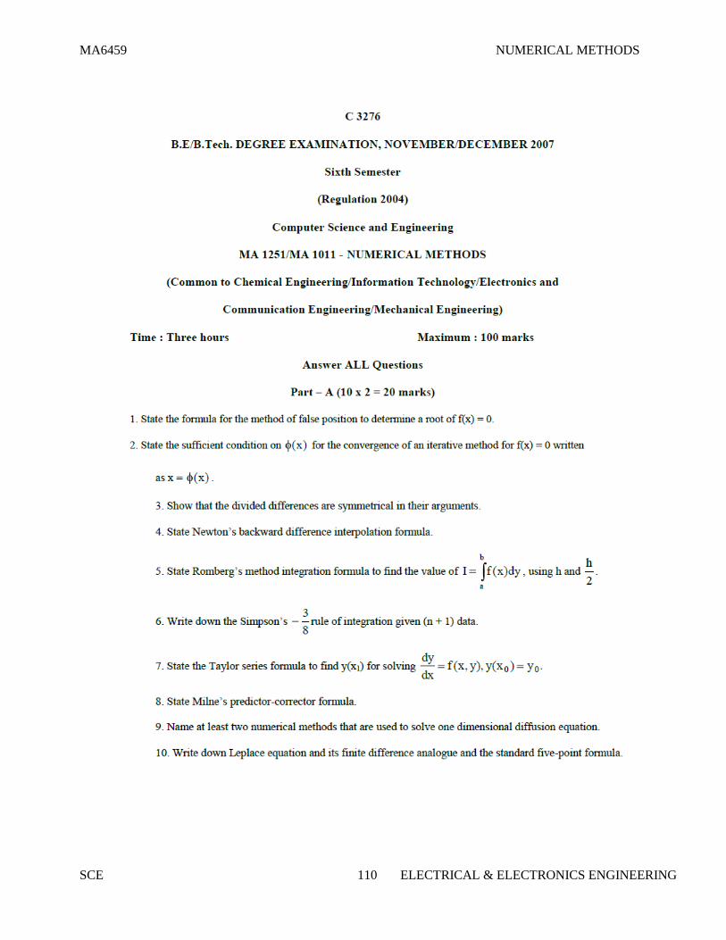
MA6459 NUMERICAL METHODS
SCE 110 ELECTRICAL & ELECTRONICS ENGINEERING

MA6459 NUMERICAL METHODS
SCE 111 ELECTRICAL & ELECTRONICS ENGINEERING

MA6459 NUMERICAL METHODS
SCE 112 ELECTRICAL & ELECTRONICS ENGINEERING
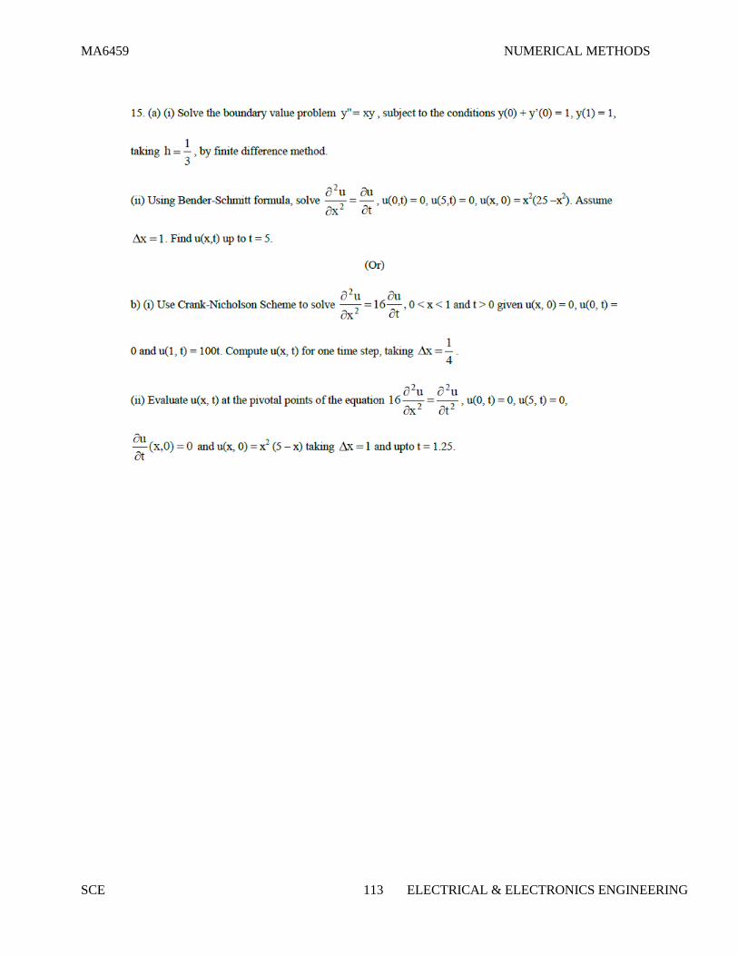
MA6459 NUMERICAL METHODS
SCE 113 ELECTRICAL & ELECTRONICS ENGINEERING

MA6459 NUMERICAL METHODS
SCE 114 ELECTRICAL & ELECTRONICS ENGINEERING
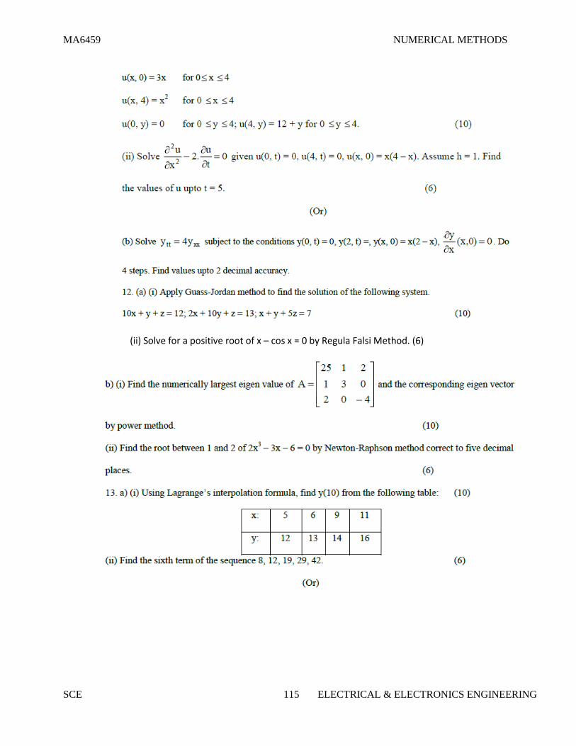
MA6459 NUMERICAL METHODS
SCE 115 ELECTRICAL & ELECTRONICS ENGINEERING
(ii) Solve for a positive root of x – cos x = 0 by Regula Falsi Method. (6)

MA6459 NUMERICAL METHODS
SCE 116 ELECTRICAL & ELECTRONICS ENGINEERING

MA6459 NUMERICAL METHODS
SCE 117 ELECTRICAL & ELECTRONICS ENGINEERING

MA6459 NUMERICAL METHODS
SCE 118 ELECTRICAL & ELECTRONICS ENGINEERING