MA3473: Mathematical Education Project

MA3473: Mathematical Education Project

Cathal Ormond: 07616520

January 24, 2011

Contents

1 Topic 2

2 History of Integration 42.1 Introduction . . . . . . . . . . . . . . . . . . . . . . . . . . . . . . . . . . . . 42.2 Pre-Calculus Integration . . . . . . . . . . . . . . . . . . . . . . . . . . . . . 42.3 Cavalieri and Fermat . . . . . . . . . . . . . . . . . . . . . . . . . . . . . . . 62.4 Newton and Leibniz . . . . . . . . . . . . . . . . . . . . . . . . . . . . . . . 62.5 Cauchy, Riemann and Darboux . . . . . . . . . . . . . . . . . . . . . . . . . 72.6 Lebesgue . . . . . . . . . . . . . . . . . . . . . . . . . . . . . . . . . . . . . . 92.7 Applications . . . . . . . . . . . . . . . . . . . . . . . . . . . . . . . . . . . . 10

3 Integration in Curricula 123.1 The Leaving Certificate . . . . . . . . . . . . . . . . . . . . . . . . . . . . . . 123.2 Chief Examiner’s Reports . . . . . . . . . . . . . . . . . . . . . . . . . . . . 163.3 Rationale . . . . . . . . . . . . . . . . . . . . . . . . . . . . . . . . . . . . . 19

4 Teaching Plan 214.1 Introduction . . . . . . . . . . . . . . . . . . . . . . . . . . . . . . . . . . . . 214.2 Unit Plan . . . . . . . . . . . . . . . . . . . . . . . . . . . . . . . . . . . . . 214.3 Unit . . . . . . . . . . . . . . . . . . . . . . . . . . . . . . . . . . . . . . . . 23

A Statistics 44A.1 Chief Examiner’s Report: Results . . . . . . . . . . . . . . . . . . . . . . . . 45A.2 Students Taking Higher Course . . . . . . . . . . . . . . . . . . . . . . . . . 46

Bibliography 47

1

Chapter 1

Topic

The topic I have chosen for this project is Integral Calculus, aimed at Leaving Certificate

students, honours level. The reason that I have chosen this topic is mostlybecause of the

marked difference in the way integral calculus was taught to me at secondary and tertiary

level. In secondary schools, integration is taught as to be a partial inverse of differentiation:

if we have f(x) and take its derivative f ′(x), then to get f(x) again (up to a constant) we

merely need to integrate f ′(x). While this is indeed true for indefinite integrals, it is only so

because of the Fundamental Theorem of Calculus. My problem with it is that it is not the

correct definition of an integral.

Integral Calculus can be defined in many ways, but almost all definitions encompass the

underlying idea of area or volume. Informally, for nice enough functions f : R → R, the

(definite) integral of f between points a and b is our concept of the “area” between the graph

of f and the x-axis, bounded by the lines x = a and x = b. We can then extend this concept

to 3 dimensions, i.e. for functions f : R×R→ R, and now our integral gives us out concept

of “volume”. In practice, we do not need to generalise this to f : Rn → R, although integral

calculus in higher dimensions is no more difficult.

I feel that teaching students that the integral is an inverse to differentiation sometimes

teaches instrumental understanding but not always relational understanding, i.e. how to in-

tegrate a function, but not what an integral actually is. It implies that integration is merely a

useful tool when working with derivatives, a mere subcategory of differential calculus which

has some interesting applications to area/volume problems. In truth, Differentiation and

Integration are two separate concepts within Calculus, which are curiously linked. I believe

2

CHAPTER 1. TOPIC

that teaching integration in terms of area and volume and then showing its applications to

differentiation teaches mathematical understanding.

Most of the above ideas, as I have stated, arise because I felt these topics were much

better explained (certainly in my experience) in third level syllabi. I would not go as far as

saying that what we were taught at Leaving Cert was incorrect, but it certainly could have

been explained better. The same, I always thought, was true of the logarithmic function

and the exponential function: their proper definition was given as a property, and a specific

property was given as their definitions. It is quite understandable, though, as the syllabus

has to be based on material taught previously, and the more rigorous definitions require a

lot of background material.

I realise that much of what I was taught in University is not possible to teach in sec-

ondary schools, due to the omission of certain areas of mathematics, for example: extrema,

continuity and certain more rigorous definitions of limits. Also, there exists the problem that

in second-level education, there are few properties of integrals that are actually proved, so

detailed explanation or definition is not required. Despite this, I intend to define integration

in my teaching plan below in terms of Riemann integration, via Darboux Sums. Then, I

will explain the link between integration and differentiation, and finally I will show some

properties of integration - including integration of algebraic and trigonometric functions -

with applications to area.

I do not believe that my method of teaching integration is too difficult for Leaving

Certificate students. The definition itself may require a lengthier introduction, but I will

not be assuming material that is not already on the course. While this teaching plan would

indeed take more time than the current way of teaching integration to Leaving Certificate

students, I feel that this method intuitively makes more sense (to me, at least) and provides

students with a better understanding of Integral Calculus.

3

Chapter 2

History of Integration

2.1 Introduction

As stated in Chapter 1 above, I will be defining it by Darboux Sums. This is because

I believe it to be the most intuitive and most practical definition of an integral short of

Lebesgue integration. The underlying theory of integration was largely worked on by Isaac

Newton and Gottfried Leibniz with the introduction of calculus in the 17th century. However,

we can see examples in many cultures of people before Newton and Leibniz determining the

areas and volumes of geometric structures - i.e. pre-calculus integration.

2.2 Pre-Calculus Integration

Before calculus was invented, there was obviously no formal idea of integration, but that

is not to say that people were not able to compute areas and volumes. Possibly the first

occurrence of integration dates back as far as 1,800 BC, when Egyptian mathematicians gave

a formula for the volume of trapezoid and the frustum of a pyramid [1]. A proof for this,

however, was not given, and was almost certainly estimated. It was not until 400 BC that

the idea was given a more rigorous treatment.

Greek Mathematicians in particular studied the idea of infinite series and approximation,

and one method they employed was the Method of Exhaustion developed by Eudoxus of Cnidus

(c 410 BC - c 355 BC). Archimedes of Syracuse (287 BC - 212 BC) used this method to ap-

proximate the area of a circle [2, p 541]. The idea was that for each n ∈ N, a polygon with

4

2.2. PRE-CALCULUS INTEGRATION CHAPTER 2. HISTORY OF INTEGRATION

n sides could be drawn both inside and outside the circle. The areas of these polygons were

calculable, and both converged to the area of the circle as the polygons gained more sides,

i.e. as n→∞.

Table 2.1: Archimedes’ method of estimating the area of a circle [3]

We can see that each polygon internal and external to the circle approximates the area of

the circle, and that as n becomes large, both areas become equal. This method is comparable

to Upper and Lower Darboux Sums. Archimedes also used the method of exhaustion to show

that the area between a parabola and a line segment is 43

times the area of a triangle with

the same base and height [4, p 68]. He did this by creating an infinite sequence of triangles:

T, T4, T16, T64, . . . where T is the required triangle, and the successive triangles lie between

T and the parabola.

Table 2.2: Archimedes’ Parabola and Triangle [3]

5

2.3. CAVALIERI AND FERMAT CHAPTER 2. HISTORY OF INTEGRATION

In the above, as we add more triangles, the total area approximates the area between the

parabola and the line. Archimedes proved that the area of Tn was equal to 1n

times the area

of T . This gives that the total area of the parabola segment is the sum of the areas of the

triangles in the sequence, so

Apar = |T |+ |T4|+ |T16|+ |T64|+ · · ·= |T |

(1 + 1

4+ 1

16+ 1

64+ · · ·

)= 4

3|T |

2.3 Cavalieri and Fermat

After Archimedes, there were not many notable Mathematicians who made significant progress

in this area of Calculus until about 1, 600. Bonaventura Cavalieri (1598 AD - 1647 AD)

worked on many geometrical problems, and while doing so unknowingly evaluated many

integrals. For example, considering a parallelogram and dividing it into two triangles by

introducing a diagonal, he proved that the area of the two triangles had to be the same, and

so each had to be half of the area of the parallelogram. In terms of calculus, this could be

written: ∫ a

0

x dx =a2

2

Using this method, the process could be generalised to integrating xn for n = 1, . . . , 9 [1],

and conjectures it so for all natural numbers [6, p149]. Pierre Fermat (1601 - 1665), however,

improved on this. He proved it for all n ∈ Q using methods which would later be similar to

that of Upper Darboux Summation. He considered the curve y = xn and evaluated the area

between x = 0 and x = a by constructing rectangles under the curve [1, p 351]. He found

that ∫ a

0

xn =an+1

n+ 1

2.4 Newton and Leibniz

The major development of integral calculus came in the 17th century with the works of

Isaac Newton (1642 - 1727) and Gottfried Leibniz (1646 - 1716) on infinitesimal calculus - an

area of calculus which considered arbitrarily small quantities. Both men are credited with

the creation of the foundations of calculus, although it remains somewhat controversial as

to who invented it first, and if one used techniques of the other. The problem was that

6

2.5. CAUCHY, RIEMANN AND DARBOUXCHAPTER 2. HISTORY OF INTEGRATION

both men were initially viewing the integral in terms of geometry as opposed to in terms of

analysis. While integration was certainly a useful technique for finding area, most - if not

all - of the integrals were worked out geometrically. There did not appear to be any method

of analytically deriving the integral of a function.

The major breakthrough came with the Fundamental Theorem of Calculus. This was

proved by James Gregory (1638 - 1675) in his book Vera Circuli et Hyperbolae Quadratura

in geometrical form [5]. Isaac Newton’s mentor Isaac Barrow (1630 - 1677) proved a more

general version of this theorem [7]. It was then that Newton and Leibniz were able to develop

the theory surrounding the theorem and in turn integral calculus. They independently

showed that if we have any function f and a differentiable function F such that F ′(x) = f(x),

then f is integrable, and moreover∫ b

a

f(x) dx = F (b)− F (a)

Once the link between integrals and anti-derivatives was established, it became possible

to integrate a wider number of functions. It was Leibniz who introduced the indefinite

integral notation

∫f(x) dx that we still use today. The symbol

∫is an elongated s,

standing for summa (Latin for sum), as integration was seen as an infinite sum of polygons.

Joseph Fourier (1768 - 1830) is credited with the limit notation

∫ b

a

f(x) dx.

2.5 Cauchy, Riemann and Darboux

While Leibniz and Newton are said to have been the pioneers of calculus, many of their

definitions encompassed and even relied on the notion of infinitesimals. Many mathemati-

cians disapproved of this, as it was not considered to be mathematically thorough. It was

Augustin Cauchy (1789 - 1857) who started the process of giving the definition of an in-

tegral a more rigorous treatment. He defined the integral as the limit of an infinite sum

[8]. In his book “Resume des lecons donnees a l’Ecole Royale Polytechnique sur le calcul

infinitesimale” (1823), Cauchy defined the integral of a continuous function f : [a, b]→ R as

follows: let a = x0 < x1 < · · · < xn = b be a partition of the interval on the real line [a, b],

7

2.5. CAUCHY, RIEMANN AND DARBOUXCHAPTER 2. HISTORY OF INTEGRATION

and denote the Cauchy Sum as

S =n∑i=1

f(xi)(xi − xi−1)

Cauchy proved that for two different partitions whose difference in norm was sufficiently

small, the corresponding Cauchy Sums could be made to differ by an arbitrarily small

amount. The integral was then the limit over all partitions. The problem with this def-

inition was that functions with discontinuities could not be integrated. Around this time,

Bernhard Riemann (1826 - 1866) had been working on the problem left by Peter Dirichlet

(1805 - 1859): what classes of functions are integrable? Unlike Cauchy, Riemann did not

require functions to be continuous - simply bounded - yet the Riemann Sum was quite sim-

ilar to the Cauchy Sum. The difference was that in each subinterval, Riemann took a point

ti ∈ [xi, xi+1], and so the Riemann Sum became

S =n∑i=1

f(ti)(xi − xi−1)

It was this small change that included functions which had some discontinuities in the defi-

nition of integrable, thus encompassing a wider range of functions. Gaston Darboux (1842 -

1917) brought the methods of Riemann to France in 1875 [9, p 22]. He also made a change

to Riemann’s definition of integrable. Given a partition P of [a, b], a bounded function

f : [a, b] → R is integrable if the Upper Darboux Sum U(f, P ) and Lower Darboux Sum

L(f, p) given by

U(f, P ) =n∑i=1

(sup

xi−1≤x≤xif(x)

)(xi − xi−1)

L(f, P ) =n∑i=1

(inf

xi−1≤x≤xif(x)

)(xi − xi−1)

have the property that

inf{U(f, P ) | P is a partition of [a, b]} = sup{L(f, P ) | P is a partition of [a, b]}

whenever these extrema exist. If f is integrable, then its integral is defined to be this value.

Darboux also showed that his definition and Riemann’s of integrable were equivalent. This

integral is often called the Riemann integral.

8

2.6. LEBESGUE CHAPTER 2. HISTORY OF INTEGRATION

2.6 Lebesgue

Towards the end of the 19th century, mathematicians began to study functions that were

called “pathological”. Generally these were functions which were not as well-behaved as

functions people generally used, for example, discontinuous functions, non-differentiable

functions etc. While Darboux Sums provided a good definition for integration, many of

these pathological functions were not integrable. Thus, mathematicians sought to redefine

the integral to include such functions. A classic example is the indicator function on the

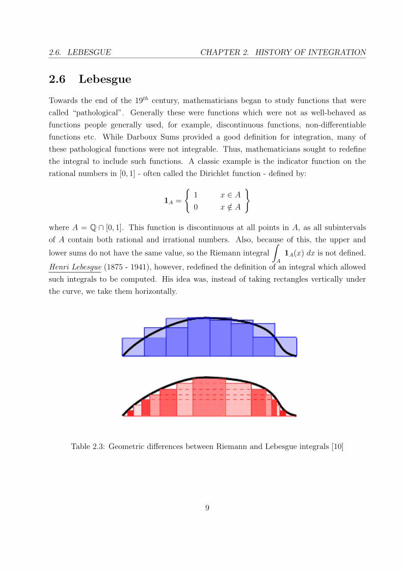
rational numbers in [0, 1] - often called the Dirichlet function - defined by:

1A =

{1 x ∈ A0 x /∈ A

}

where A = Q ∩ [0, 1]. This function is discontinuous at all points in A, as all subintervals

of A contain both rational and irrational numbers. Also, because of this, the upper and

lower sums do not have the same value, so the Riemann integral

∫A

1A(x) dx is not defined.

Henri Lebesgue (1875 - 1941), however, redefined the definition of an integral which allowed

such integrals to be computed. His idea was, instead of taking rectangles vertically under

the curve, we take them horizontally.

Table 2.3: Geometric differences between Riemann and Lebesgue integrals [10]

9

2.7. APPLICATIONS CHAPTER 2. HISTORY OF INTEGRATION

This (with admittedly quite a bit of measure theory) allowed us to define the Lebesgue

integral. Thus, in the above integral, we have∫A

1A(x) dx =

∫A

1A dµ = 1 · µ(Q ∩ [0, 1]) + 0 · µ(R \ (Q ∩ [0, 1])) = 0

where µ is the Lebesgue measure on R. Lebesgue went on to show that if a function was

Riemann integrable, then it was also Lebesgue integrable, and the two integrals were the

same.

2.7 Applications

The applications of integration are wide and varied. If we have a region D in Rn, then∫D

dn~x is the n-dimensional volume of D. Furthermore, if we have a function f : Rn → R,

then

∫D

f(x) dn~x is the n-dimensional volume under the curve of f within D. Practically,

we can use these to find areas and volumes. As mentioned above, practically (especially for

non-mathematicians) we usually consider the n = 2, 3 cases and ignore the rest.

In other areas of mathematics, we can extend the idea of integrating over the real line,

to integrating over curves (line integrals) and surfaces (surface integrals). We can also

define integration in the complex plane. When integrating over C, many improper integrals

(i.e. integrals over infinite sets or with unbounded integrands) are much easier to solve, for

example we can show: ∫ ∞−∞

1

1 + x2= π

by integrating over a particular path in C. Integrals are used frequently in Fourier Analysis.

The Fourier transform of an integrable function f is denoted f , and has the relation

f(k) =

∫ ∞−∞

f(x)e−2πikx dx f(x) =

∫ ∞−∞

f(k)e2πikx dk

In more mathematics, however, we have that the length of the curve of a function y = f(x)

between the points (a, c) and (b, d) is given by either of the following

∫ b

a

√1 +

(dy

dx

)dx

∫ d

c

√1 +

(dx

dy

)dy

10

2.7. APPLICATIONS CHAPTER 2. HISTORY OF INTEGRATION

Also, the average value of a function f : [a, b]→ R is given by

1

b− a

∫ b

a

f(x) dx

Integration has many application in the fields of Physics and Statistics. If we know that the

path of a particle can be described by a function f : [a, b] → R, then the integral of f over

[a, b] is the work done in moving the particle from a to b. Consider a solid beam of length

L with density by p(x) at a point x on the beam. Then, the centre of mass of the beam is

given by

x =

∫ L

0

xp(x) dx∫ L

0

p(x) dx

We can extend this to 3-dimensional objects, and we get the centroid of the object.

In statistics, given a specific probability distribution X, if we have a continuous function

FX which tells us the probability of an event occurring, then the probability density func-

tion is given by

fX(x) =

∫ x

−∞FX(t) dt

Furthermore, given a probability distribution with PDF (X, pX), the average value of X is

given by

µX = E(X) =

∫ ∞−∞

tfX(t) dt

and the variance is given by

σ2X = Var(X) =

∫ ∞−∞

(t− µX)2fX(t) dt

11

Chapter 3

Integration in Curricula

Given my target age group for this teaching plan, I will be examining the development

of integration within the Irish Leaving Certificate Curriculum. Firstly, I will give a brief

description of the changes in the Honours Leaving Certificate Mathematics course in general,

and then deal specifically with changes in the Integral Calculus syllabus. It will be convenient

to group the following syllabus revisions by the following five phases (similar to [11, p 9]):

1924-68, 1968-77, 1977-94, 1994 - 2010, 2010 onwards. I have chosen these particular years

because of the changes in the integral calculus section of the syllabus, not strictly because

of the syllabus revisions themselves. I will also discuss the Chief Examiner’s Reports for the

years 2005, 2000, and 1995, and finally will give my rationale for including Integration in

the Leaving Certificate Curriculum.

3.1 The Leaving Certificate

3.1.1 Phase 1: 1924-68

The first major standardisation of the mathematics curriculum came with the foundation of

the Irish Free state in 1922, and up until the 1960’s, very little change was made to it [11,

p 8]. The Leaving Certificate Mathematics Course (like most other courses) was split into

Pass course and an Honours course. The primary aim behind the Leaving Certificate itself

was “to testify to the completion of a good secondary education and the fitness of a pupil

to enter on a course of study at a University or an educational institute of similar standing”

[12, p 9], an aim that did not change for almost 50 years.

12

3.1. THE LEAVING CERTIFICATE CHAPTER 3. INTEGRATION IN CURRICULA

This particular syllabus initially contained two different Mathematics courses: Pro-

gramme A and Programme B. Each programme was examined by three papers: Arithmetic,

Algebra and Geometry/Trigonometry. Programme A was the standard Leaving Certificate

Mathematics course that would go on to run for many years. The Leaving Certificate section

of Programme B was “intended to give a thorough training in elementary Mathematics which

[would] prepare the future engineer or scientific worker for his subsequent mathematical and

scientific studies” [12, p 22]. In particular, the latter programme included differential calcu-

lus which the former programme did not.

The integration syllabus on the first phase of the mathematics course was quite similar

to the syllabus of the fourth phase (1994 - 2010) below. The examinable material included

“derivatives and integrals of elementary functions (Algebraic and Trigonometric) with easy

applications to problems on rates, tangents, areas, volumes and to problems of motion” [12,

p 20]. Students were expected to be able to solve definite and indefinite integrals involving

polynomials and trigonometric functions, evaluate area/volume problems etc. This was only

examined on Programme A; there was no calculus on Programme B. These two programmes

were examined until the 33/34 Academic Year, after which one, combined Mathematics

Syllabus was adopted, incorporating aspects from both of the previous two syllabi [13, p 24].

As mentioned above, this syllabus remained almost entirely unchanged until 1968. The only

change was that of wording in 1935: “Introduction to the differential and integral calculus.

Derivatives and integrals of simple algebraic and trigonometric functions, with applications”

[13, p 25].

3.1.2 Phase 2: 1968 - 77

This syllabus went almost entirely unchanged until the mid 1960’s when the Department of

Education introduced new material (“Modern Mathematics”) into the Leaving Certificate

Syllabus [11, p 8]. The new syllabus was examined by only two papers [14, p 60]. Most of

the content of the previous Arithmetic paper was removed [11, p 10], including all areas of

calculus. Some differential calculus was added to the Pass Course syllabus, a topic which

had not been included in this syllabus before. The syllabus saw several changes (partly due

to the syllabus changes in the Intermediate Certificate at the time) until the 1970’s.

13


In the 1971/72 Academic Year, the Leaving Certificate was seen in a new light. The aim

of the course was “to prepare pupils for immediate entry into open society or for proceeding

to further education” [15, p 29], admittedly only a slight change from the previous aim. The

syllabus underwent radical changes during this period, with all calculus being reinstated.

Concepts such as matrices and linear transformations were introduced, and areas like Taylor

Series and polar coordinates were reduced [11, p 10-11].

In the 1972/72 Academic Year, all previous elements of integral calculus became exam-

inable again, including some integrals not seen before, for example:

•∫

dx

q(x), where q(x) is a quadratic polynomial

•∫ekx dx, where k ∈ R

•∫

dx

x2 + a2,

∫ √a2 − x2 dx,

∫dx√

a2 − x2, where a ∈ R

Also, integration by parts was introduced for functions such as log x, xekx, sinmx, etc.

The applications of the definite integral were the same, namely area under curves. This

marked the biggest change in the integration syllabus since Phase 1, and most of the material

introduced in this syllabus revision is currently still examinable.

3.1.3 Phase 3: 1977 - 94

It was noted that the Higher syllabus was quite long, and may have been focussing to much

on applications of mathematics instead of some more basic pure mathematics. [11, p 11-12].

To try and obviate this, the course was again modified somewhat. Before, there had been an

option of Groups and Probability. Under the new syllabus, students had the choices between

Statistics or Vectors/Linear Transformations and between the Geometry of Parabolas and

Groups. This phase saw few changes in the integral calculus syllabus. Integration by parts

was removed entirely. Also, integration of rational functions was not examinable, while

integration of polynomials in general was [16, p 166]. This syllabus remained unchanged

until 1994.

14


3.1.4 Phase 4: 1994 - 2010

In the 1993/94 Academic Year, the syllabus changed into the format with which students

(certainly of my generation, at least) are currently most familiar, with the course still be-

ing examined by two papers. The core subjects were Algebra, Geometry/Trigonometry,

Sequences and Series, Functions and Calculus and Discrete Mathematics/Statistics. These

subjects were examined on Paper 1 and Section A of Paper 2. Section B of Paper 2 contained

four questions (one of which to be attempted) on the optional subjects: Further Calculus

and Series, Further Probability and Statistics, Groups and Further Geometry. [17, p 9-16].

The major change in terms of integration was the reintroduction of integration by parts into

the syllabus, but to include it and its applications as part of the options questions (Section

B, Paper 2) under Further Calculus and Series. No more than two steps are required for the

integration by parts itself. [17, p 16].

3.1.5 Phase 5: 2010 Onwards

The New Mathematics syllabus (called Project Maths) contains 5 different strands, splitting

the course as follows:

• Strand 1: Statistics and Probability

• Strand 2: Geometry and Trigonometry

• Strand 3: Numbers

• Strand 4: Algebra

• Strand 5: Functions

In September 2010, the first two strands of the Project Maths syllabus (Probability and

Geometry/Trigonometry) were introduced into schools nationwide, and will be examinable

in 2012 [18, p 10]. There will still be two papers for this exam, comprising of the two strands,

a separate geometry course, and some material retained from the previous syllabus. For the

moment, all areas of integral calculus are being retained.

Paper 1 will have three sections: Section A (Concepts and Skills), Section B (Contexts

and Applications), and Section C (Functions and Calculus) [19]. Section C will be based on

material from the 1994 Mathematics Syllabus. Paper 2 will have two sections: Section A

(Concepts and Skills) and Section B (Contexts and Applications) [20].

15

3.2. CHIEF EXAMINER’S REPORTS CHAPTER 3. INTEGRATION IN CURRICULA

3.2 Chief Examiner’s Reports

3.2.1 1995

This was the second year that the 1994 Syllabus was examined, and while there was a slight

decrease in students taking Mathematics overall, the percentage of students who took the

Higher paper increased from 11.2% in 1993 to 16.8% in 1995. See the appendix for a graph

of the results during this period.

Paper 1

In Paper 1, Question 8 (Integral Calculus) was the 4th most popular question attempted,

based on a sample of 4% of the total scripts. Students attained a mean mark of 38 out of

50, the second best answered question on the paper. It is reported that this question was

in general well attempted [21, p 12]. A problem which arose was that students often forgot

to put in the limits of integration, despite the fact that the indefinite integral was usually

correct. In the final section of part (c), “there were few correct attempts made to derive the

required volume”. [21, p 12]

Paper 2

In Paper 2, Section B, Question 8 (Further Calculus and Series) was the most popular

question attempted (88% of candidates), based on a sample of 4% of the total scripts. This

question was “managed very well by candidates” [21, p 15]

3.2.2 2000

In 1997, the new syllabus tentatively introduced in 1992 was finalised. The Higher and

Ordinary courses were examined as introduced in 1994, and the Foundation course replaced

the previous Alternative Ordinary course (which was introduced in 1990) in 1997. The

percentages of students who took the Higher paper from 1996 to 2000 were as follows: 17.8%

in 1996, 18.1% in 1997, 17.3% in 1998, 17.6 in 1999 and 18.1 in 2000. See the appendix for

a graph of the results during the period 1998 - 2000.

16


Paper 1

In Paper 1, Question 8 (Integral Calculus) was the 5th most popular question attempted

(94% of candidates), based on a sample of 4% of the total scripts. Students attained a mean

mark of 37 out of 50, the second best answered question on the paper [22, p 4].

For part (a), the constant of integration was remembered more so in this year than in

previous years, and full marks were given to students frequently. The main problem in

section (b) was that students sometimes misused the formulae given in the Mathematical

Tables. In (c)(i), students either got full marks or none. Once the trick of completing the

square was noticed, the integral was correctly evaluated, whereas students who did not see

this method tended not to score any marks. Very few students managed to correctly evaluate

(c)(ii), which was a question on area requiring some algebra [22, p 8-9].

Paper 2

In Paper 2, Section B, Question 8 (Further Calculus and Series) was the most popular ques-

tion attempted (95% of candidates), based on a sample of 4% of the total scripts. Students

attained a mean mark of 28 out of 50, which was the lowest average of mark in this section

[22, p 4].

In (b)(i), integration by parts was required twice to correctly evaluate the indefinite

integral. The first application of integration by parts was dealt with well, and full marks

were given to most students. The second application gave some problems with students

incorrectly evaluating the integrals. This resulted in most candidates getting an attempt

mark. Part (b)(ii) relied on substituting limits for the previous integral. Students who

successfully evaluated the first section had no problem with the second, but the majority of

candidates had an incorrect result due to mistakes in the first section [22, p 14].

Comments

The Chief Examiner noted that students’ strengths in integral calculus was mainly in inte-

gration not requiring substitution [22, p 16], but recognised that students’ weaknesses lay

mainly in applying integration to evaluate area and volume problems. [22, p 17].

17


3.2.3 2005

The percentages of students who took the Higher paper from 2001 to 2005 were as follows:

18% in 2001, 17.6% in 2002, 17.4% in 2003, 17.8% in 2004, 18.9% in 2005. See the appendix

for a graph of the results during the period 2003 - 2005.

Paper 1

In Paper 1, Question 8 (Integral Calculus) was the 6th most popular question attempted

(85% of candidates), based on a sample of 4% of the total scripts. Students attained a mean

mark of 35 out of 50, the joint second best answered question on the paper (joint with 3

other questions). It is reported that this question was in general well attempted [23, p 55].

For part (a), almost all students were able to perform basic integration, and remembered

the constant of integration. In section (b)(i), most students recognised the logarithmic

integral, and evaluated it correctly. Errors occurred when students substituted incorrect

limits. Students who use the Mathematical Tables to evaluate∫

sin2 x dx directly tended to

make more mistakes than students who used trigonometric formula to write the integrand

in terms of cos. In (c)(i), few students noticed the trick of completing the square, and even

those that did tended to make mistakes with the algebra as opposed to the calculus. Very

few students managed to evaluate (c)(ii), a question on deriving the volume of a cone [23, p

62].

Paper 2

In Paper 2, Section B, Question 8 (Further Calculus and Series) was the most popular

question attempted (95% of candidates), based on a sample of 4% of the total scripts.

Students attained a mean mark of 37 out of 50, which was the second highest (and also

second lowest) average of mark in this section. [23, p 55] The integration by parts question

(a) was generally answered very well. The biggest problem was students forgetting the

constant of integration. [23, p 68]

Comments

The Chief Examiner noted that students’ strengths in integral calculus was mainly in inte-

gration (with or without substitution) of elementary functions and integration by parts [23,

18

3.3. RATIONALE CHAPTER 3. INTEGRATION IN CURRICULA

p 73], but recognised that students’ weaknesses lay mainly in integration when the form is

not familiar (e.g. competing the square). [22, p 17].

3.3 Rationale

I believe that the inclusion of integral calculus in the Leaving Certificate Honours syllabus

is justified. As detailed above in Section 3.1, integration has been included in the Leaving

Certificate Syllabus almost consistently from 1924 to the present. Given their close link, it

is often taught directly after differential calculus, and indeed differentiation is regularly used

in integral calculus. Integration can be seen as a link from Geometry to Calculus, and so

students can verify some of their own integrals by geometric means.

The Chief Examiner’s Reports in Section 3.2 above show that on Paper 1, while Question

8 (Integration) is not always one of the more popular questions, students tend to answer it

well enough (on average 37 marks out of 50). The main problems students have is making

small mistakes (algebra or sometimes differentiation), omitting the constant of integration or

sometimes not noticing a trick that will evaluate the integral simply (completing the square).

In general, students seem to be quite apt at straightforward integration and substitution,

so the topic itself, unlike areas such as Sequences and Series or Statistics, seems to be well

understood. In fact, despite the frequent use of differentiation in integral calculus, students

on average tend to score slightly higher in the integration question than in either of the two

differentiation questions.

The main section with which students tend to struggle is Area and Volume. Students

seem not to be able to relate their knowledge of indefinite integration to that of area and

volume. This is seen in the Chief Examiners Reports in Section 3.2 above. I feel, however,

that as the most well known (and indeed, for non-mathematicians, often the most useful)

application of integral calculus is finding volumes and area, I feel that this subject not only

needs to remain on the curriculum, but also perhaps needs to be taught in a new light to

students understand area and volumes problems better.

I mentioned above that the current methods of teaching integration is not, in my opinion,

the best way of teaching it, and that while students may know how to integrate, few will

know what an integral actually is. Many people would say that, practically speaking, this

19

3.3. RATIONALE CHAPTER 3. INTEGRATION IN CURRICULA

suffices. In courses like engineering and science, students are not required to know what the

underlying theory of integrals are, so what is the point in teaching it? Why go to such an

effort to explain something that will not be used?

Aside from the fact that this is an aim of the Leaving Cert [17, p 4] and is correct

mathematical rigour (for the background material covered), this method of teaching integral

calculus can help show students that many areas of mathematics are linked, and it reinforces

the notion that students can use techniques from other areas of maths as long as they are

mathematically correct. Also, it encourages students to see try to find links themselves

within mathematics. These skills are quite transferable to other subjects also.

20

Chapter 4

Teaching Plan

4.1 Introduction

I mentioned in my introduction that I intend to teach integration in terms of area and Dar-

boux Sums. I gave the reason that I feel that this definition may make more intuitive sense,

and is the correct method of defining an integral. It was noted in the Chief Examiner’s

Reports that some students, while able to evaluate basic integrals and use most techniques

of integration, tend to have problems working out the area under curves. This was noted in

particular in 2005 [23, p 62].

I believe that by teaching students integration via area, they may have a better intuitive

grasp of how to derive areas and volumes. The Fundamental Theorem of Calculus will be

used to justify the integrals which are too difficult to evaluate geometrically. I will not (an

indeed cannot at this level) go into rigorous detail with the definition, but I will be assuming

some prior knowledge of infinite sequences (ignoring convergence). Similarly, I will not be

proving the Fundamental Theorem of Calculus (at least, not in any great detail), as its proof

is not required on the Leaving Certificate course.

4.2 Unit Plan

In this unit, I intent to cover all material required to answer a full question on integration

in the Leaving Certificate Honours Paper. The syllabus I have in mind is the one adopted

21

4.2. UNIT PLAN CHAPTER 4. TEACHING PLAN

in 1992, as the current syllabus is changing.

Prior Knowledge

The unit is aimed at students in the Senior Cycle Course, so all relevant material from the

Junior Cycle will be assumed. It is expected that students will have covered the following

areas of the Senior Cycle: Sequences and Series (although a detailed knowledge will not be

required), Differential Calculus, Trigonometry and Limits.

Unit Layout

This unit is (approximately) set to run for two and a half weeks, i.e. 12 periods, with an in

class test at the end of the unit. There will be five classes a week, each lasting 40 minutes.

Students will be presented with homework questions regularly, from both the book, and

then from past papers when they have covered sufficient material. It will have the following

provisional layout: (sections marked with (∗) will be formal lesson plans, while the others

will be mini-plans)

Week 1 Week 2

Day 1 Definition of the Integral (∗) Day 1 log x and ex

Day 2 FTC and Linearity (∗) Day 2 Trigonometric Integrals

Day 3 Substitution 1 Day 3 Substitution 2

Day 4 Trigonometric Functions and Substitution Day 4 Substitution 2 (∗)Day 5 Trigonometric Functions, log x and ex Day 5 Applications to Area

Week 3

Day 1 Application to Area (∗)Day 2 Review of Unit: Past Paper Questions

Day 3 In Class Test

Day 4

Day 5

Teaching and Resources

The primary resources for this unit will be the book, the past papers. As stated many

times above, my idea is to introduce the integral as the area beneath a curve and to relate

integration to differentiation by the Fundamental Theorem of Calculus. This method is not

22

4.3. UNIT CHAPTER 4. TEACHING PLAN

entirely unfamiliar in modern curricula. A brief outline of how the area under the curve of

a function is related to the derivative of that function is outlined in the Leaving Certificate

book Teacs & Trialacha 5 [24, p 51-52].

I will begin with some basic functions whose graphs resemble shapes that we have con-

sidered before in geometry, e.g. rectangles and triangles. This will mean that students will

be able to guess the value of an integral and then on evaluating it check their answer. After

the definition and before the applications of integrals, I will be regularly noting the link

between differentiation and integration, and will use techniques with which students should

be already familiar.

The main resources that I will be using in the classroom will be the textbook (either

of the chapters [25, Ch 14] or [24, Ch 2]) and the Past Examination Papers. The majority

of the work during class will be done on the blackboard, and occasionally handouts will be

given to the students. It will be assumed that the class has the following attributes:

Class Name 5A

No. of Students 25

Characteristic of Class Able

Class Length 40 mins

Subject Mathematics: Higher Level

Topic Integral Calculus

The various mini plans will be more basic than the detailed lesson plans. They will

assume a prior knowledge of the previous class unless otherwise specified.

4.3 Unit

4.3.1 Lesson Plan 1: Lesson 1

Prior Knowledge

This is a new topic within Calculus. It requires students to be familiar with functions,

summation notation and limits.

23


Content and Skills

Concept and definition of an integral.

Principal Aim

Students will understand how the area between a curve and the x-axis may be calculated

via Darboux Sums.

Behavioural Objectives

At the end of the class, students should be able to do simple examples involving:

• evaluating integrals by geometric methods

Activities

Introduction

The class is told they are going to link geometry to calculus. Introduce the definition of Up-

per and Lower Darboux sum, and explain pictorially what the definition means (rectangles

above/below the curve).

The value (xi − xi−1) is the width of a rectangle, and the value max f(x) and min f(x) rep-

resent the heights of the upper and lower rectangles respectively. Thus, max f(x)(xi− xi−1)and max f(x)(xi− xi−1) are the area of each of the rectangles, and then we sum these areas

to get the total area. Define the definite integral to be the common value of the sums when

the rectangles become infinitely narrow.

Note that in the definition of Darboux sums, we change the extrema to maxima and

minima. Introduce the notation of

∫ b

a

f(x) dx for integral. Stress that dx term only means

“with respect to x”. Also, this method of evaluating integrals should be likened to differen-

tiation from first principles: it is the definition and works in most simple cases, but it is not

the method that will be commonly employed in integration.

24


Development

Presentation 1

Question: Can we relate this to something we already know?

Answer : Geometry - the area of familiar shapes. We can find functions whose graphs are

shapes we know, and hence whose areas we have been given before.

Application 1

On the blackboard, consider the constant function f(x) = 2, and evaluate

∫ 10

0

f(x) dx. This

graph represents a rectangle, so we know that the integral should be 20 units2. Choose any

partition of [a, b]. As the function is constant, the values max f(x) and min f(x) are constant

also, and hence equal. This gives us:

U(f, P ) =n∑i=1

(max

xi−1≤x≤xif(x)

)(xi − xi−1) = 2

n∑i=1

(xi − xi−1) = 2(10− 0)

L(f, P ) =n∑i=1

(min

xi−1≤x≤xif(x)

)(xi − xi−1) = 2

n∑i=1

(xi − xi−1) = 2(10− 0)

noting the telescoping series. The upper and lower sums are the same, and give us the value

we want. Note that we chose values for f(x), a and b, but we could have easily solved this

without them, so in fact: ∫ b

a

c dx = c(b− a)

Application 2 Again, on the blackboard, consider the function f(x) = x. If we look at

the line x = 10, the shape formed is a right-angled triangle. We will compute the integral∫ 10

0

f(x) dx. We know that the integral should give us

Area =1

2(10)(10) = 50 units2

The function is increasing, so we have

maxxi−1≤x≤xi

f(x) = f(xi) = xi minxi−1≤x≤xi

f(x) = f(xi−1) = xi−1

25


We’ll take a specific partition of [0, 10]:

x0 = 0, x1 =10

n, x2 =

20

n, . . . , xi =

10i

n, . . . , xn =

10n

n= 10

We can conclude that

U(f, P ) =100

n2

(n∑i=1

i

)L(f, P ) =

100

n2

(n−1∑j=0

j

)

(this method was taken from [26, p 258-260]). Students will recall thatm∑k=0

k =m∑k=1

k =

m(m+ 1)

2. This gives us

L(f, P ) =n(n− 1)

2

100

n2=n− 1

n50 U(f, P ) =

n(n+ 1)

2

100

n2=n+ 1

n50

We know (or at least have a good idea), a priori, that this function can be integrated, as we

have determined the area beneath the curve by other means. We can determine the value of

the integral in two ways. Firstly, it is now hard to prove that

n− 1

n≤ 1 ≤ n+ 1

n

for all n ∈ N. This gives us

L(f, P ) ≤ 50 ≤ U(f, P )

Similarly, we could consider what happens when we let n→∞, namely when the rectangles

in our particular partition get infinitely narrow.

limn→∞

L(f, P ) = limn→∞

n− 1

n50 = 50 lim

n→∞U(f, P ) = lim

n→∞

n+ 1

n50 = 50

Thus, the (unique) value of the integral is given by∫ 10

0

x dx = 50 units2

which we expected.

26


Conclusion

Question class to check behavioural objectives.

Homework:

• Confirm that

∫ b

0

x dx =b2

2and hence

∫ b

a

x dx =b2

2− a

2

2. Also, evaluate

∫ 10

0

(x+2) dx

both geometrically (from the graph) and analytically (evaluating the integral).

• Consider the function f(x) = x2 and the integral∫ 3

0f(x). Compute the Upper and

Lower sums for the integral given the following partitions: {0, 3}, {0, 1.5, 3}, {0, 1, 2, 3}.Tell students that the area should work out to be 9 units2

4.3.2 Lesson Plan: Lesson 2

Prior Knowledge

This is the second class on the new topic of Integral Calculus. Students should be familiar

with the definition of a definite integral and should be able to evaluate some integrals.

Students should recall simple differentiation.

Content and Skills

Finding anti-derivatives, and solving more general integrals.

Principal Aim

Students will be able to link their knowledge of differentiation to integration to solve more

integrals.


At the end of the class, students should be able to:

• find anti-derivatives

• evaluate integrands of the form xn for n ∈ Z \ {−1}

• do examples involving the linearity of integrals

27


Activities

Introduction

Go through some of the homework from the previous night. Recall from the previous class

the definition of an integral, and remind students that we know the following∫ b

a

c dx = c(b− a)

∫ b

a

x dx =b2

2− a2

2

Development

Presentation 1

Question: Can we use the same process as before to evaluate∫ bax2 dx?

Answer : Yes, but it becomes more tricky. Also, we do not have an elementary geometric

method of finding the area of a parabola, so we cannot check our answer. The previous

homework question should show at (at least heuristically) that the method is still valid. So

how should we proceed?

There exists a link between Differentiation and Integration, given by The Fundamental

Theorem of Calculus (FTC). If we wish to evaluate

∫ b

a

f(x) dx and can find some g(x) such

that g′(x) = f(x) for all x ∈ [a, b], then∫ b

a

f(x) dx = g(b)− g(a) = g(x)∣∣x=bx=a

We can see this as follows. Let g(t) be the area under the curve between f(x) and the

x− axis bounded by the lines x = a and x = t, i.e.

g(t) =

∫ t

a

f(x) dx

Leth > 0, and consider the two points x and x+h. If we look at the term (g(x+h)− g(x)),

this is the area under f(x) bounded by x and x+h. Approximately, this is equal to the area

of a rectangle under the curve. Mathematically this is

g(x+ h)− g(x) ≈ h · f(x) ⇔ g(x+ h)− g(x)

h≈ f(x)

28


If we let h→ 0, we have

g′(x) = f(x)

and also

g(b)− g(a) =

∫ b

a

f(x) dx−∫ a

a

f(x) dx =

∫ b

a

f(x) dx

as required. (This is proven in detail here [26, Ch 14]). We note that

d

dx

(xn+1

n+ 1

)= xn

whenever n 6= 1 so we are not dividing by 0. Let f(x) = xn and g(x) = xn+1

n+1This gives us,

by the FTC ∫ b

a

xn dx = g(b)− g(a) =bn+1

n+ 1− an+1

n+ 1

If we let n = 0, 1, we can test that this agrees with the integrals we evaluated previously.

Application 1

Using the blackboard, evaluate the integral

∫ b

a

x2 dx, and show that the integral from the

previous homework (when a = 0, b = 3) does indeed evaluate to 9 units2. Try some more

difficult integrals, for example: ∫ 2

−1x3 dx

∫ 1

0

x4 dx

Presentation 2

Question: What about polynomials in general? Can we integrate them?

Answer : Yes, because integrals are linear.

Recall for series that if a1, a2, . . . , an and b1, b2, . . . , bn are sequences and c ∈ R, then we

know thatn∑i=1

(ai + bi) =n∑i=1

ai +n∑i=1

bi

n∑i=1

c · an = c ·n∑i=1

an

As integrals are defined in terms of sums, the same is true for integration: if f(x) and g(x)

are functions and c ∈ R, then∫ b

a

(f(x) + g(x)) dx =

∫ b

a

f(x) +

∫ b

a

g(x) dx

∫ b

a

c · f(x) dx = c ·∫ b

a

f(x) dx

29


Application 2

Try some simple examples like∫ 1

02x− 1 dx. Exercises from the book.

Conclusion

Recap on material covered in class: FTC and linearity of integrals.

4.3.3 Mini Plan: Lesson 3

Content and Skills

Indefinite integrals. Integration by substitution.

Principal Aim

Students will be able to find a general formula for the area under the curve, independent

of limits. Students will be shown how to manipulate integrals so that they are in a more

recognisable (and hence more easily integrable) format.

Activities

Introduction

Note that we may not know what the limits for integration are, and it is not convenient to

keep writing g(b)− g(a). Introduce indefinite integrals. Recall the chain rule from differen-

tiation. We will use similar processes to integration.

Development

Presentation 1

If we wanted to evaluate∫

(x + 1)4 dx, we could expand using the binomial theorem, but

this will lead to many tedious calculations. When working on differentiation, we substituted

u = x+ 1 and then we said thatdy

dx=dy

du· dudx

, which was easier than expansion. The same

can be done with integrals, with a slight difference.

Application 1

30


Evaluating the above, we let u = x+ 1, sodu

dx= 1, or rearranging du = dx. Thus,

∫(x+ 1)4 dx =

∫u4 du =

u5

5+ c =

(x+ 1)5

5+ c

remembering to re-substitute x = u+ 1. Try another simple example from the book.

Presentation 2

Sometimes, regardless of the substitution du 6= α · dx for some constant α. In this case,

we simply express x in terms of u and substitute. The idea is that after substitution, out

integral should be easier to solve.

Application 2

For example, in∫x√x2 + 1 dx, we can let u = x2 + 1, so du = 2x dx. This gives∫

x√x2 + 1 dx =

1

2

∫ √u du =

1

4√u

+ c =1

4√x2 + 1

+ c

Go through some more examples from the book.

Conclusion

Recap on substitution. Homework problems from book.


Prior Knowledge

Trigonometric formulae and identities. Integration by substitution

Content and Skills

Integration of trigonometric functions

31


Principal Aim

Students will be able to integrate algebraic functions of the familiar trigonometric functions,

in particular products and power of sin and cos.

Activities

Introduction

From differential calculus, we know the derivatives of some trigonometric functions. We can

apply this to the integrals of the same functions.

Development

Presentation 1

We know that (sinx)′ = cosx and (cos x)′ = − sinx, so∫sinx dx = − cosx+ c

∫cosx dx = sinx+ c

Application 1

Some examples from the book, including trigonometric formulae. Evaluate integrals of the

form∫

sinmx cosnx dx,∫

sin2 x dx and∫

cos2 x dx.

Presentation 2

If we have an integral of the form∫

sin2 x cosx dx, we cannot use trigonometric formulae to

solve. We can, however, use the substitution u = sinx, so du = cosx dx. Thus, the integral

is easier to solve.

Application 2

Questions from the book.

Conclusion

Recap on integration of trigonometric functions and substitution, and set homework from

book.

32



Prior Knowledge

Previous class on integration of trigonometric functions. The Exponential and logarithmic

functions.

Content and Skills

Integration of the exponential and logarithmic functions.

Principal Aim

Students will recall integration of substitution and will be able to do simple examples in-

volving integration of the exponential and trigonometric functions.

Activities

Introduction

Go through homework. Recall the integrals of the trigonometric functions. Further examples.

Development

Presentation 1

Recall from differentiation that the function f(x) = ex has the property that f ′(x) = f(x).

This gives us that∫ex dx = ex + c.

Application 1

Some examples from the book with integrands of the form f(x) = ceax+b.

Presentation 2

Recall also from differentiation that the function f(x) = log x has the property that f ′(x) =1x. This gives us that

∫dxx

= log |x|+ c, where the absolute values remind students that log x

where x < 0 is undefined.

Application 2

Go through examples form the book with integrands of the form f(x) =c

log(ax+ b).

33


Conclusion

Recap on material covered in class. Assignment given out in class, to do over the weekend.

Material taken from past papers based on topics covered in previous week.


Prior Knowledge

Previous week on integration.

Content and Skills

Further integration of logarithmic and exponential functions.

Principal Aim

Collect assignment, to be marked and graded for the next class (if possible). Students will

be reminded of techniques of substitution, and will learn how to apply them to various

compositions of trigonometric functions, log x and ex. Students will also become familiar

with logarithmic integration.

Activities

Introduction

Collect assignment handed out last lesson. Recall previous rules of integrals of trigonometric

functions, of log x and of ex.

Development

Presentation 1

We can now use the previous week to evaluate more complicated integrals, say of the form

f(x) = 2xex2.

Application 1

Questions from the book.

34


Presentation 2

Recall that for some functions y = f(x), we considered log y = log(f(x)), and used im-

plicit differentiation to solve fordy

dx. We will use an analogous method for evaluating some

integrals. For example, if we wish to evaluate∫2x+ 1

x2 + x+ 3dx

there is no readily available method. However, if we let u = x2 +x+3, then du = (2x+1)dx,

so the integral is simply evaluated. Note that the trick we used was to note that s∫f ′(x)

f(x)dx = log |f(x)|+ c

Application 2

Examples from the book, including trigonometric functions.

Conclusion

Recap on material covered in class. Homework questions


Prior Knowledge

Inverse trigonometric functions.

Content and Skills

Trigonometric integrals.

Principal Aim

Students will be able to evaluate integrals of the form:∫dx

a2 + x2

∫dx√

a2 − x2

35


Activities

Introduction

Recall that we can integrate functions of the form f(x) =1

ax+ b. However, when the

denominator becomes a quadratic and we cannot integrate by logarithms, we have a problem.

Development

Presentation 1

Introduce first trigonometric integral:∫dx

x2 + a2=

1

atan−1

x

a+ c

Use the substitution x = a tan θ, and deduce this result.

Application 1

Questions from the book, and simple substitution which reduces to this form.

Presentation 2

Introduce second trigonometric integral:∫dx√

a2 − x2= sin−1

x

a+ c

Use the substitution x = a sin θ, and deduce this result.

Application 2

Questions from the book, and simple substitution which reduces to this form.

Conclusion

Recap on results, set homework from the book.


Prior Knowledge

Previous classes on integration.

36


Content and Skills

Further integration by substitution.

Principal Aim

Students will learn further techniques of substitution which will enable them to reduce an in-

tegral to one of the forms they are familiar with. In particular, we will deal with substitutions

of the form x = a sin θ or x = a cos θ.

Activities

Introduction

Development

Presentation 1

While we can evaluate integrals of the form∫ √

c± x dx for constants c ∈ R, but integrals

of the form∫ √

c± x2 dx pose a problem. If we consider (what at a higher level we would

call a change of coordinates) the substitution x = a sin θ, we can solve the integrals more

readily. Application 1

Examples from the book.

Conclusion

Recap on material from class. Homework from book and past papers.


Prior Knowledge

Students have been studying integration for over a week at this stage, and should be familiar

with integrating polynomials, trigonometric and some inverse trigonometric functions, log x

and ex, including basic integration by substitution.

Content and Skills

Further integration by substitution: Completing the Square.

37


Principal Aim

Students will further their knowledge of substitution, and will thus be able to evaluate a

wider number of functions.


At the end of this class, students will be able to

• complete the square for general quadratic trinomials

• use this “trick” to reduce complicated integrals into trigonometric.

Activities

Introduction

Recall that we could solve rational functions whose denominators were of the form x2 + a2,

but for general quadratic trinomials, we do not necessarily have a solution. The method of

completing the square will help us.

Development

Presentation 1

We wish to write a general quadratic trinomial x2+bx+c in the form (x+h)2+k. (Note that

the coefficient of x2 was deliberately left out, as we can factor it out later on). Expanding,

we have

x2 + bx+ c = x2 + 2hx+ h2 + k

and equating, this gives

h =b

2k = c− b2

4

This gives us

x2 + bx+ c =

(x+

b

2

)2

+

(c− b2

4

)which we can verify easily.

Application 1

38


We now use the above in integrals. Say we wish to evaluate∫dx

x2 + 4x+ 13

After short consideration, it is clear that there isn’t much we can do in terms of logarithmic

or trigonometric integration, so we must substitute. We will complete the square, and then

reconsider our integral. By above, we have that h = 2 and k = 13 − 4 = 9, so now our

integral becomes ∫dx

x2 + 4x+ 13=

∫dx

(x+ 2)2 + 9=

∫dx

(x+ 2)2 + 32

Note that this is almost in a form we recognise. We use the substitution u = x+ 2, and this

evaluates easily enough to∫du

u2 + 32=

1

3tan−1

(u3

)+ c =

1

3tan−1

(x+ 2

3

)+ c

as required.

Application 2

We’ll consider the following ∫ 3

2

2

x2 − 6x+ 10dx

Completing the square gives us∫2

x2 − 6x+ 10dx = 2

∫dx

(x− 3)2 + s1

We make the substitution u = x− 3, so∫2

x2 − 6x+ 10dx = 2

∫1

(x− 3)2 + 12dx = 2 tan−1(x− 3) + c

and hence ∫ 3

2

2

x2 − 6x+ 10dx = 2[tan−1(x− 3)]32 = 2

[π −

(−π

4

)]=

5π

2

39


Conclusion

Recap on material from class, stressing the algebraic trick involved. Remind students that

we can use other areas of mathematics when integrating.


Prior Knowledge

Previous classes on integration and some geometry.

Content and Skills

Applications to Area.

Principal Aim

Students will recall the definition of an integral and use this to evaluate area via integration.

Activities

Introduction

Remind students that we began by defining the integral of a function as the area between the

curve and the x-axis, bounded by the lines x = a and x = b. Now we have many techniques

that will allow us to calculate area without resorting to Darboux sums.

Development

Presentation 1

For example, if we want to find the area under the curve of f(x) = sinx between 0 and π,

then we evaluate∫ π0

sin(x) dx = 2. However, if we try the area between −π and 0, we get

−2, so the area between −π and π is 0. This is obviously not true, as an area exists. Thus,

when calculating area, we will take absolute values if our function goes under the x-axis.

Application 1

Go through some examples from the book.

Presentation 2

Note that a circle centred around the origin of radius r is given by x2 + y2 = r2. Rewriting

40


this, we have y = ±√r2 − x2 , where the positive values gives the upper half and the negative

value gives the lower half.

Application 2

To calculate the area of the circle, we consider f(x) =√r2 − x2 , and integrate it between

−r and r. This will give the area of a semi-circle, so the area of a circle will be

Acirc = 2

∫ r

−r

√r2 − x2 dx

We use the substitution x = r sin θ, we have

2r2∫ π/2

−π/2cos2 θ dθ = πr2

as required.

Conclusion

Recap on material from class. Give assignment to class to do over the weekend comprising

of material from pas papers.


Prior Knowledge

Students are almost at the end of the unit, so should be very familiar with techniques of

integration.

Content and Skills

Applications to Area: Spheres and Revolutions

Principal Aim

Students will develop their concept of volume using integration.


At the end of this lesson, students should be able to

41


• calculate the volume attained when a graph is rotated around an axis.

• calculate the volume of a sphere.

Activities

Introduction

Introduce the idea of generalisation of area to volume. Show the formulae of the volume of

a solid attained by rotating the function y = f(x) around the x-axis and x = g(y) around

the y-axis, i.e.

Vx = π

∫ b

a

y2 dx Vy = π

∫ b

a

x2 dy

Development

Presentation 1

Go through some simple examples with familiar functions rotated around the axes.

Presentation 2

Go through the derivation of the volume of a cone.

Conclusion

Recap on material from lesson. Let students know that the next lesson will be entirely exam

practise with questions from past papers, and the lesson after that will be a test on the unit.


Prior Knowledge

Students have reached the end of the unit. They should be familiar with integrals and their

evaluation.

Principal Aim

At the end of this lesson, students will be comfortable with exam questions relation to

integral calculus.

42


Activities

Go through an entire question from the paper, and begin another if time allows.

43

A.1. CHIEF EXAMINER’S REPORT: RESULTS APPENDIX A. STATISTICS

Appendix A

Statistics

A.1 Chief Examiner’s Report: Results

45

A.2. STUDENTS TAKING HIGHER COURSE APPENDIX A. STATISTICS

A.2 Students Taking Higher Course

46

Bibliography

[1] Carl B. Boyer, A History of Mathematics, Wiley, 1991.

[2] Reviel Netz, The Works of Archimedes, Cambridge University Press, 2004

[3] http://www.storyofmathematics.com/hellenistic archimedes.html

[4] W.W. Rouse Ball, A Short Account of the History of Mathematics, Dover Publications,

1960.

[5] Marlow Anderson, Victor J. Katz, Robin J. Wilson, Sherlock Holmes in Babylon: and

other Tales of Mathematical History, The Mathematical Association of America, 2004.

[6] John Stillwell, Mathematics and its History Springer, 2002.

[7] J. M. Child, The Geometrical Lectures of Isaac Barrow, The Open Court Publishing

Company, 1916.

[8] Thomas Hawkins, Lebesgue’s Theory of Integration - its Origins and Development,

Chelsea Publishing Company, 1975.

[9] Douglas S. Kurtz, Theories of Integration, World Scientific Publishing Company, 2004.

[10] http://en.wikipedia.org/wiki/File:RandLintegral.png

[11] Elizabeth E. Oldham, SIMS: Report on the Irish National Committee Trinity College

Dublin, 1976.

[12] An Roinn Oideachais, Brainse an Mhean-Oideachais, Programme and Regulations re-

garding Curricula, Certifications, Examinations and Scholarships, Stationary Office,

1924.

47

BIBLIOGRAPHY BIBLIOGRAPHY



1935.



1968.



1971.



1977.

[17] An Roinn Oideachais, Brainse an Mhean-Oideachais, The Leaving Certificate: Mathe-

matics Syllabus, Stationary Office, 1994.

[18] Department of Education and Skills, Mathematics Syllabus: Foundation, Ordinary and

Higher Level. For Examination in 2012 Only, 2010.

[19] State Examinations Commission, Leaving Certificate Examination 2011: Mathematics

Paper 1 (Sample Paper) 2010.

[20] State Examinations Commission, Leaving Certificate Examination 2011: Mathematics

Paper 2 (Sample Paper) 2010.

[21] State Examinations Commission, Leaving Certificate Examination: Chief Examiner’s

Report, Department of Education, 1995.





[24] O. D. Morriss and P. Cooke, Teacs & Trialacha 5: An Mhatamaitic (Ardleibheal) An

Gum, 1994.

48

BIBLIOGRAPHY BIBLIOGRAPHY

[25] George Humphrey, New Concise Maths 4: Leaving Cert Higher Level (Part 1), Gill &

Macmillan, 2003.

[26] Michael Spivak, Calculus, Publish or Perish, 1994.

49

MA3473: Mathematical Education Project

Documents

Transcript of MA3473: Mathematical Education Project