MA2AA1 (ODE’s): Lecture Notes

Sebastian van Strien (Imperial College)

Spring 2015 (updated from Spring 2014)

Contents0 Introduction i

0.1 Practial Arrangement . . . . . . . . . . . . . . i0.2 Relevant material . . . . . . . . . . . . . . . . ii0.3 Notation and aim of this course . . . . . . . . . iii0.4 Examples of differential equations . . . . . . . iv0.5 Issues which will be addressed in the course

include: . . . . . . . . . . . . . . . . . . . . . v

1 Existence and Uniqueness: Picard Theorem 11.1 Banach spaces . . . . . . . . . . . . . . . . . . 11.2 Metric spaces . . . . . . . . . . . . . . . . . . 21.3 Metric space versus Banach space . . . . . . . 21.4 Examples . . . . . . . . . . . . . . . . . . . . 31.5 Banach Fixed Point Theorem . . . . . . . . . . 51.6 Lipschitz functions . . . . . . . . . . . . . . . 61.7 The Picard Theorem for ODE’s (for functions

which are globally Lipschitz) . . . . . . . . . . 71.8 Application to linear differential equations . . . 91.9 The Picard Theorem for functions which are

locally Lipschitz . . . . . . . . . . . . . . . . . 11

1.10 Some comments on the assumptions in Picard’sTheorem . . . . . . . . . . . . . . . . . . . . . 13

1.11 Some implications of uniqueness in Picard’sTheorem . . . . . . . . . . . . . . . . . . . . . 14

1.12 Higher order differential equations . . . . . . . 151.13 Continuous dependence on initial conditions . . 161.14 Gronwall Inequality . . . . . . . . . . . . . . . 161.15 Consequences of Gronwall inequality . . . . . 171.16 The butterfly effect . . . . . . . . . . . . . . . 181.17 Double pendulum . . . . . . . . . . . . . . . . 18

2 Linear systems in Rn 192.1 Some properties of exp(A) . . . . . . . . . . . 202.2 Solutions of 2× 2 systems . . . . . . . . . . . 222.3 n linearly independent eigenvectors . . . . . . 232.4 Complex eigenvectors . . . . . . . . . . . . . . 252.5 Eigenvalues with higher multiplicity . . . . . . 262.6 A worked example: 1 . . . . . . . . . . . . . . 262.7 A second worked example . . . . . . . . . . . 282.8 Complex Jordan Normal Form (General Case) . 302.9 Real Jordan Normal Form . . . . . . . . . . . 31

3 Power Series Solutions 323.1 Legendre equation . . . . . . . . . . . . . . . 323.2 Second order equations with singular points . . 333.3 Computing invariant sets by power series . . . 36

4 Boundary Value Problems, Sturm-Liouville Prob-lems and Oscillatory equations 384.1 Motivation: wave equation . . . . . . . . . . . 384.2 A typical Sturm-Liouville Problem . . . . . . . 444.3 A glimpse into symmetric operators . . . . . . 464.4 Oscillatory equations . . . . . . . . . . . . . . 49

5 Calculus of Variations 515.1 Examples (the problems we will solve in this

chapter): . . . . . . . . . . . . . . . . . . . . . 515.2 Extrema in the finite dimensional case . . . . . 535.3 The Euler-Lagrange equation . . . . . . . . . . 545.4 The brachistochrone problem . . . . . . . . . . 575.5 Are the critical points of the functional I minima? 625.6 Constrains in finite dimensions . . . . . . . . . 62

5.6.1 Curves, surfaces and manifolds . . . . 625.6.2 Minima of functions on constraints (man-

ifolds) . . . . . . . . . . . . . . . . . . 645.7 Constrained Euler-Lagrange Equations . . . . . 65

6 Nonlinear Theory 676.1 The orbits of a flow . . . . . . . . . . . . . . . 676.2 Singularities . . . . . . . . . . . . . . . . . . . 686.3 Stable and Unstable Manifold Theorem . . . . 686.4 Hartman-Grobman . . . . . . . . . . . . . . . 736.5 Lyapounov functions . . . . . . . . . . . . . . 746.6 The pendulum . . . . . . . . . . . . . . . . . . 776.7 Hamiltonian systems . . . . . . . . . . . . . . 786.8 Van der Pol’s equation . . . . . . . . . . . . . 796.9 Population dynamics . . . . . . . . . . . . . . 84

7 Dynamical Systems 877.1 Limit Sets . . . . . . . . . . . . . . . . . . . . 877.2 Local sections . . . . . . . . . . . . . . . . . . 887.3 Planar Systems . . . . . . . . . . . . . . . . . 907.4 Poincaré Bendixson . . . . . . . . . . . . . . . 927.5 Consequences of Poincaré-Bendixson . . . . . 937.6 Further Outlook . . . . . . . . . . . . . . . . . 94

Appendices 96

Appendix A Multivariable calculus 96A.1 Jacobian . . . . . . . . . . . . . . . . . . . . . 96A.2 The statement of the Inverse Function Theorem 98A.3 The Implicit Function Theorem . . . . . . . . . 101

Appendix B Prerequisites 103B.1 Function spaces . . . . . . . . . . . . . . . . . 103

Appendix C Explicit methods for solving ODE’s 104C.1 State independent . . . . . . . . . . . . . . . . 104C.2 State independent x = f(t). . . . . . . . . . . 104C.3 Separation of variables . . . . . . . . . . . . . 105C.4 Linear equations x′ + a(t)x = b(t). . . . . . . 106C.5 Exact equations M(x, y)dx + N(x, y)dy = 0

when ∂M/∂y = ∂N/∂x. . . . . . . . . . . . . 106C.6 Substitutions . . . . . . . . . . . . . . . . . . 107C.7 Higher order linear ODE’s with constant coef-

ficients . . . . . . . . . . . . . . . . . . . . . . 108C.8 Solving ODE’s with maple . . . . . . . . . . . 111C.9 Solvable ODE’s are rare . . . . . . . . . . . . 112C.10 Chaotic ODE’s . . . . . . . . . . . . . . . . . 112

Appendix D A proof of the Jordan normal form theo-rem 113

0 Introduction

0.1 Practial Arrangement• The lectures for this module will take place Wednesday

9-11, Thursday 10-11 in Clore.

• Each week I will hand out a sheet with problems. It isvery important you go through these thoroughly, as thesewill give the required training for the exam and classtests.

• Support classes: Thursday 11-12, from January 22.

• The support classes will be run rather differently fromprevious years. The objective is to make sure that youwill get a lot out of these support classes.

• The main way to revise for the tests and the exam is bydoing the exercises.

• There will be two class tests. These will take place onTuesday 9th February and Tuesday 9th March. Each ofthese count for 5% .

• Questions are most welcome, during or after lecturesand during office hour.

• My office hour is to be agreed with students reps. Officehour will in my office 6M36 Huxley Building.

i

0.2 Relevant material• There are many books which can be used in conjunction

to the module, but none are required.

• The lecture notes displayed during the lectures will beposted on my webpage: http://www2.imperial.ac.uk/~svanstri/ Click on Teaching in the leftcolumn. The notes will be updated during the term.

• The lectures will also be recorded. See my webpage.

• There is no need to consult any book. However, recom-mended books are

– Simmons + Krantz, Differential Equations: The-ory, Technique, and Practice, about 40 pounds. Thisbook covers a significant amount of the material wecover. Some students will love this text, others willfind it a bit longwinded.

– Agarwal + O’Regan, An introduction to ordinarydifferential equations.

– Teschl, Ordinary Differential Equations and Dy-namical Systems. These notes can be downloadedfor free from the authors webpage.

– Hirsch + Smale (or in more recent editions): Hirsch+ Smale + Devaney, Differential equations, dynam-ical systems, and an introduction to chaos.

– Arnold, Ordinary differential equations. This bookis an absolute jewel and written by one of the mas-ters of the subject. It is a bit more advanced thanthis course, but if you consider doing a PhD, thenget this one. You will enjoy it.

Quite a few additional exercises and lecture notes can befreely downloaded from the internet.

ii

0.3 Notation and aim of this course

Notation: when we write x then we ALWAYS meandx

dt. When

we write y′ then this usually meansdy

dxbut also sometimes

dy

dt;

which one should always be clear from the context.This course is about studying differential equations of the

typex = f(x), resp. y = g(t, y)

which is short for finding a function t 7→ x(t) (resp. t 7→ y(t))so that

dx

dt= f(x(t)) resp.

dy

dt= g(y, y(t)).

In particular this means that (in this course) we will assume

thatdx

dtis continuous and therefore t 7→ x(t) differentiable.

Aim of this course is to find out when or whether such anequation has a solution and determine its properties.

iii

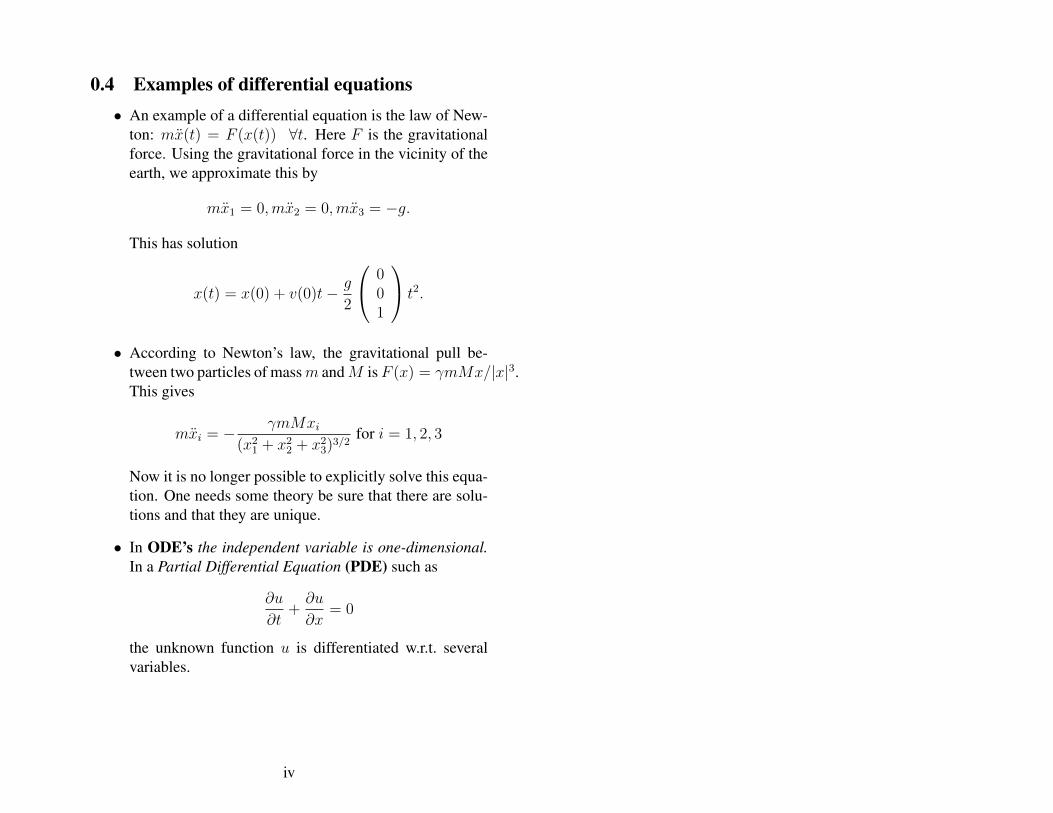
0.4 Examples of differential equations• An example of a differential equation is the law of New-

ton: mx(t) = F (x(t)) ∀t. Here F is the gravitationalforce. Using the gravitational force in the vicinity of theearth, we approximate this by

mx1 = 0,mx2 = 0,mx3 = −g.

This has solution

x(t) = x(0) + v(0)t− g

2

001

t2.

• According to Newton’s law, the gravitational pull be-tween two particles of massm andM isF (x) = γmMx/|x|3.This gives

mxi = − γmMxi(x2

1 + x22 + x2

3)3/2for i = 1, 2, 3

Now it is no longer possible to explicitly solve this equa-tion. One needs some theory be sure that there are solu-tions and that they are unique.

• In ODE’s the independent variable is one-dimensional.In a Partial Differential Equation (PDE) such as

∂u

∂t+∂u

∂x= 0

the unknown function u is differentiated w.r.t. severalvariables.

iv

• The typical form for the ODE is the following initialvalue problem:

dx

dt= f(t, x) and x(0) = x0

where f : R × Rn → Rn. The aim is to find somecurve t 7→ x(t) ∈ Rn so that the initial value problemholds. When does this have solutions? Are these solu-tions unique?

• An example of an ODE related to vibrations of bridges(or springs) is the following (see Appendix C, Subsec-tion C.7):

Mx′′ + cx′ + kx = F0 cos(ωt).

One reason you should want to learn about ODE’s is:

– http://www.ketchum.org/bridgecollapse.html

– http://www.youtube.com/watch?v=3mclp9QmCGs

– http://www.youtube.com/watch?v=gQK21572oSU

0.5 Issues which will be addressed in the courseinclude:

• do solutions of ODE’s exist?

• are they unique?

• most differential equations, cannot be solved explicitly.One aim of this course is to develop methods which al-low information on the behaviour of solutions anyway.

v

1 Existence and Uniqueness: Picard The-orem

In this chapter we will prove a theorem which gives sufficientconditions for a differential equation to have solutions. Beforestating this theorem, we will cover the background needed forthe proof of this theorem. In this chapter X will denote a space of functions (so in-

finitely dimensional).

1.1 Banach spaces• A vector space X is a space so that if v1, v2 ∈ X thenc1v1 + c2v2 ∈ X for each c1, c2 ∈ R (or, more usually,for each c1, c2 ∈ C).

• A norm on X is a map || · || : X → [0,∞) so that

1. ||0|| = 0, ||x|| > 0 ∀x ∈ X \ {0}.2. ||cx|| = |c|||x|| ∀c ∈ R and x ∈ X3. ||x+y|| ≤ ||x||+ ||y|| ∀x, y ∈ X (triangle inequal-

ity).

• A Cauchy sequence in a vector space with a norm is asequence (xn)n≥0 ∈ X so that for each ε > 0 there existsN so that ||xn − xm|| ≤ ε whenever n,m ≥ N .

• A vector space with a norm is complete if each Cauchysequence (xn)n≥0 converges, i.e. there exists x ∈ X sothat ||xn − x|| → 0 as n→∞.

• X is a Banach space if it is a vector space with a normwhich is complete.

1

1.2 Metric spaces• A metric space X is a space with together with a func-

tion d : X ×X → R+ (called metric) so that

1. d(x, x) = 0 and d(x, y) = 0 implies x = y.

2. d(x, y) = d(y, x)

3. d(x, z) ≤ d(x, y) + d(y, z) (triangle inequality).

• A sequence (xn)n≥0 ∈ X is called Cauchy if for eachε > 0 there exists N so that d(xn, xm) ≤ ε whenevern,m ≥ N .

• The metric space is complete if each Cauchy sequence(xn)n≥0 converges, i.e. there exists x ∈ X so that d(xn, x)→0 as n→∞.

1.3 Metric space versus Banach space• Given a norm || · || on a vector space X one can also

define the metric d(x, y) = ||y − x|| on X . So a Banachspace is automatically a metric space. A metric space isnot necessarily a Banach space.

2

1.4 ExamplesExample 1. Consider R with the norm |x|. You have see inAnalysis I that this space is complete.

In the next two examples we will consider Rn with twodifferent norms. As is usual in year ≥ 2, we write x ∈ Rn

rather than x for a vector.

Example 2. Consider the space Rn and define |x| =√∑n

i=1 x2i

where x is the vector (x1, . . . , xn). It is easy to check that|x| is a norm (the main point to check is the triangle inequal-ity). This norm is usually referred to as the Euclidean norm (asd(x, y) = |x− y| is the Euclidean distance).

Typo correctedExample 3. Consider the space Rn and the supremum norm|x| = maxni=1 |xi| (it is easy to check that this is a norm).

Regardless which of two two norms we put on Rn, in bothcases the space we obtain is complete (this follows from Ex-ample 1).

Without saying this explicitly everywhere, in this course,we will always endow Rn with the Euclidean metric. In otherlectures, you will also come across other norms on Rn (for ex-ample the lp norm (

∑ni=1 |xi|p)1/p, p ≥ 1.

Example 4. One can define several norms on the space of n×nmatrices. One, which is often used, is the matrix norm ||A|| =supx∈Rn\{0}

|Ax||x| whenA is a n×nmatrix. Here x,Ax are vec-

tors and |Ax|, |x| are the Euclidean norms of these vectors. By

linearity of A we have supx∈Rn\{0}|Ax||x| = supx∈Rn,|x|=1 |Ax|

and so the latter also defines ||A||. In particular ||A|| is a finitereal number.

3

Now we will consider a compact interval I and the vectorspace C(I,R) of continuous functions from I to R. In the nexttwo examples we will put two different norms on C(I,R). Inone case, the resulting vector is complete and in the other it isnot.

Example 5. The set C(I,R) endowed with the supremum Remark: in this course it will suffice that you know thatC(I,Rn) with the supremum norm is complete - it is notnecessary to know the proof of this fact.

norm ||x||∞ = supt∈I |x(t)|, is a Banach space. That || · ||∞ isa norm is easy to check, but the proof that ||x||∞ is complete ismore complicated and will not proved in this course (this resultis shown in the metric spaces course).

Example 6. The space C([0, 1],R) endowed with the L1 norm||x||1 =

∫ 1

0|x(s)| ds is not complete.

(Hint: To prove this norm is not complete, use the sequenceof functions xn(s) = min(

√n, 1/

√s) for s > 0 and xn(0) =√

n. That this sequence is Cauchy is easy to see: for m > n

then∫ 1

0|xn(s)−xm(s)| ds =

∫ 1/m

0|√m−√n| ds+

∫ 1/n

1/m|1/√s− Typo, n > m corrected into m > n.√

n| ds ≤ 1/√m+2/

√n ≤ 3/

√n→ 0. Assume by contradic-

tion that the sequence xn converges: then there exists a contin-uous function x ∈ C([0, 1],R) so that ||x− xn||1 converges tozero. Since x is continuous, there exists k so that |x(s)| ≤

√k Indeed, for n ≥ k and s ∈ [0, 1/k), we have xn(s)−x(s) ≥

xn(s)−√k > 0. Hence ||xn−x|| ≥

∫ 1/k

0|xn(s)−x(s)|ds ≥∫ 1/k

0xn(s) − (1/k)

√k ≥ (1/n)

√n + (2/

√k − 2/

√n) −

(1/k)/√k ≥ 1/(2

√k) when n is large.

for all s. Then it is easy to show that ||xn−x|| ≥ 1/(2√k) > 0

when n is large (check this!). So the Cauchy sequence xn doesnot converge.

Remark: The previous two examples show that the same setcan be complete w.r.t. one metric and incomplete w.r.t. to an-other metric.

4

1.5 Banach Fixed Point TheoremThe proof of this theorem shows that whatever x0 youchoose the sequence xn defined by xn+1 = F (xn) con-verges to a fixed point p (and this fixed point does not de-pend on the starting point x0.

Theorem 1 (Banach Fixed Point Theorem). Let X be a com-plete metric space and consider F : X → X so that there existsλ ∈ (0, 1) so that

d(F (x), F (y)) ≤ λd(x, y) for all x, y ∈ X

Then F has a unique fixed point p:

F (p) = p.

Proof. (Existence) Take x0 ∈ X and define (xn)n≥0 by xn+1 =F (xn). This is a Cauchy sequence:

d(xn+1, xn) = d(F (xn), F (xn−1)) ≤ λd(xn, xn−1).

Hence for each n ≥ 0, d(xn+1, xn) ≤ λnd(x1, x0). Thereforewhen n ≥ m, d(xn, xm) ≤ d(xn, xn−1) + · · ·+d(xm+1, xm) ≤(λn−1 +· · ·+λm)d(x1, x0) ≤ λm/(1−λ)d(x1, x0). So (xn)n≥0

is a Cauchy sequence and has a limit p. As xn → p one hasF (p) = p. Here we use F (xn) = xn+1 → p (since xn → p) and also

F (xn) → F (p) (since d(F (xn), F (p)) ≤ λd(xn, p) → 0.Since a convergent sequence has only one limit, it followsthat F (p) = p.

(Uniqueness) If F (p) = p and F (q) = q then d(p, q) =d(F (p), F (q)) ≤ λd(p, q). Since λ ∈ (0, 1), p = q.

Remark: Since a Banach space is also a complete metric space,the previous theorem also holds for a Banach space.

Example 7. Let g : [0,∞) → [0,∞) be defined by g(x) =(1/2)e−x. Then g′(x) = (1/2)e−x ≤ 1/2 for all x ≥ 0 and sothere exists a unique p ∈ R so that g(p) = p. (By the Mean

Value Theoremg(x)− g(y)

x− y = g′(ζ) for some ζ between x, y.

Since |g′(ζ)| ≤ 1/2 for each ζ ∈ [0,∞) this implies that g is acontraction. Also note that g(p) = p means that the graph of gintersects the line y = x at (p, p).)

5

1.6 Lipschitz functionsLetX be a Banach space. Then we say that a function f : X →X is Lipschitz if there exists K > 0 so that

||f(x)− f(y)|| < K||x− y||.

Example 8. Let A be a n × n matrix. Then Rn 3 x 7→ Ax ∈Rn is Lipschitz. Indeed, |Ax − Ay| ≤ K|x − y| where K is

the matrix norm of A defined by ||A|| = supx∈Rn\{0}|Ax||x| .

Remember that ||A|| is also equal to maxx∈Rn;|x|=1 |Ax|.

Example 9. The function R 3 x 7→ x2 ∈ R is not Lipschitz:there exists no constant K so that |x2 − y2| ≤ K|x− y| for allx, y ∈ R.

Example 10. On the other hand, the function [0, 1] 3 x 7→x2 ∈ [0, 1] is Lipschitz.

Example 11. The function [0, 1] 3 x 7→ √x ∈ [0, 1] is notLipschitz.

Example 12. Let U be an open set in Rn and f : U → R becontinuously differentiable. Then f : C → R is Lipschitz forany compact set C ⊂ U . When n = 1 this follows from theMean Value Theorem, and for n > 1 this will be proved inAppendix A.

6

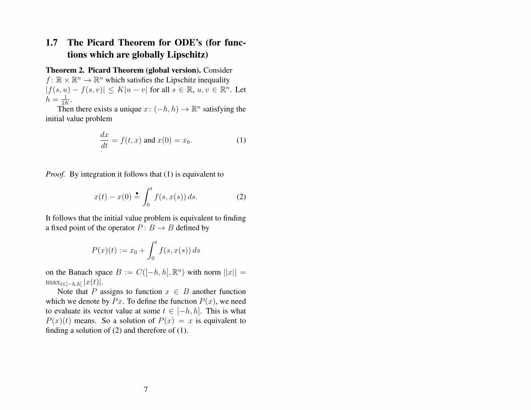
1.7 The Picard Theorem for ODE’s (for func-tions which are globally Lipschitz)

Theorem 2. Picard Theorem (global version). Considerf : R× Rn → Rn which satisfies the Lipschitz inequality|f(s, u) − f(s, v)| ≤ K|u − v| for all s ∈ R, u, v ∈ Rn. Leth = 1

2K.

Then there exists a unique x : (−h, h)→ Rn satisfying theinitial value problem

dx

dt= f(t, x) and x(0) = x0. (1)

Proof. By integration it follows that (1) is equivalent to

x(t)− x(0)•=

∫ t

0

f(s, x(s)) ds. (2)

It follows that the initial value problem is equivalent to findinga fixed point of the operator P : B → B defined by

P (x)(t) := x0 +

∫ t

0

f(s, x(s)) ds

on the Banach space B := C([−h, h],Rn) with norm ||x|| =maxt∈[−h,h] |x(t)|.

Note that P assigns to function x ∈ B another functionwhich we denote by Px. To define the function P (x), we needto evaluate its vector value at some t ∈ [−h, h]. This is whatP (x)(t) means. So a solution of P (x) = x is equivalent tofinding a solution of (2) and therefore of (1).

7

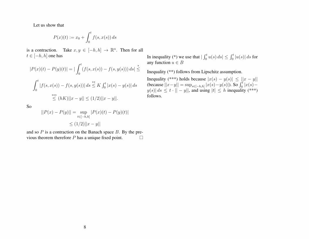
Let us show that

P (x)(t) := x0 +

∫ t

0

f(s, x(s)) ds

is a contraction. Take x, y ∈ [−h, h] → Rn. Then for allIn inequality (*) we use that |

∫ t0u(s) ds| ≤

∫ t0|u(s)| ds for

any function u ∈ B

Inequality (**) follows from Lipschitz assumption.

Inequality (***) holds because |x(s) − y(s)| ≤ ||x − y||(because ||x−y|| = sups∈[−h,h] |x(s)−y(s)|). So

∫ t0|x(s)−

y(s)| ds ≤ t · || − y||, and using |t| ≤ h inequality (***)follows.

t ∈ [−h, h] one has

|P (x)(t)− P (y)(t)| = |∫ t

0

(f(s, x(s))− f(s, y(s))) ds|∗≤

∫ t

0

|f(s, x(s))− f(s, y(s))| ds∗∗≤ K

∫ t0|x(s)− y(s)| ds

∗∗∗≤ (hK)||x− y|| ≤ (1/2)||x− y||.

So||P (x)− P (y)|| = sup

t∈[−h,h]

|P (x)(t)− P (y)(t)|

≤ (1/2)||x− y||and so P is a contraction on the Banach space B. By the pre-vious theorem therefore P has a unique fixed point.

8

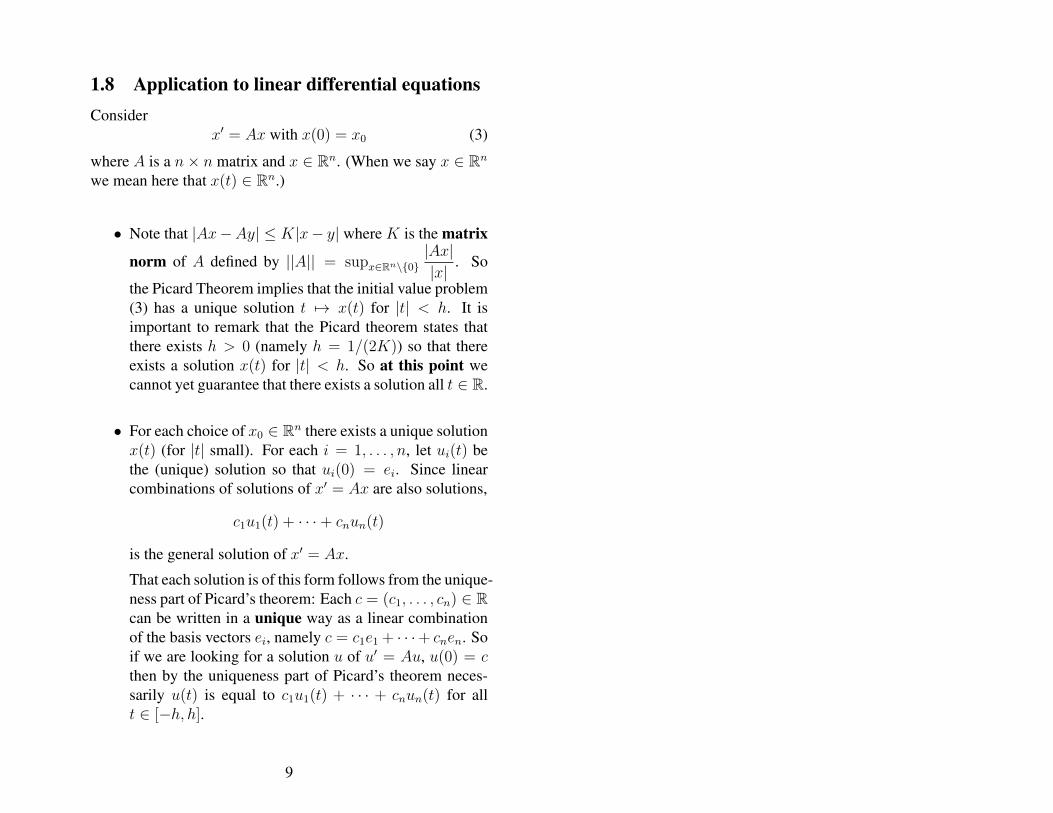
1.8 Application to linear differential equationsConsider

x′ = Ax with x(0) = x0 (3)

where A is a n× n matrix and x ∈ Rn. (When we say x ∈ Rn

we mean here that x(t) ∈ Rn.)

• Note that |Ax−Ay| ≤ K|x− y| where K is the matrix

norm of A defined by ||A|| = supx∈Rn\{0}|Ax||x| . So

the Picard Theorem implies that the initial value problem(3) has a unique solution t 7→ x(t) for |t| < h. It isimportant to remark that the Picard theorem states thatthere exists h > 0 (namely h = 1/(2K)) so that thereexists a solution x(t) for |t| < h. So at this point wecannot yet guarantee that there exists a solution all t ∈ R.

• For each choice of x0 ∈ Rn there exists a unique solutionx(t) (for |t| small). For each i = 1, . . . , n, let ui(t) bethe (unique) solution so that ui(0) = ei. Since linearcombinations of solutions of x′ = Ax are also solutions,

c1u1(t) + · · ·+ cnun(t)

is the general solution of x′ = Ax.

That each solution is of this form follows from the unique-ness part of Picard’s theorem: Each c = (c1, . . . , cn) ∈ Rcan be written in a unique way as a linear combinationof the basis vectors ei, namely c = c1e1 + · · ·+ cnen. Soif we are looking for a solution u of u′ = Au, u(0) = cthen by the uniqueness part of Picard’s theorem neces-sarily u(t) is equal to c1u1(t) + · · · + cnun(t) for allt ∈ [−h, h].

9

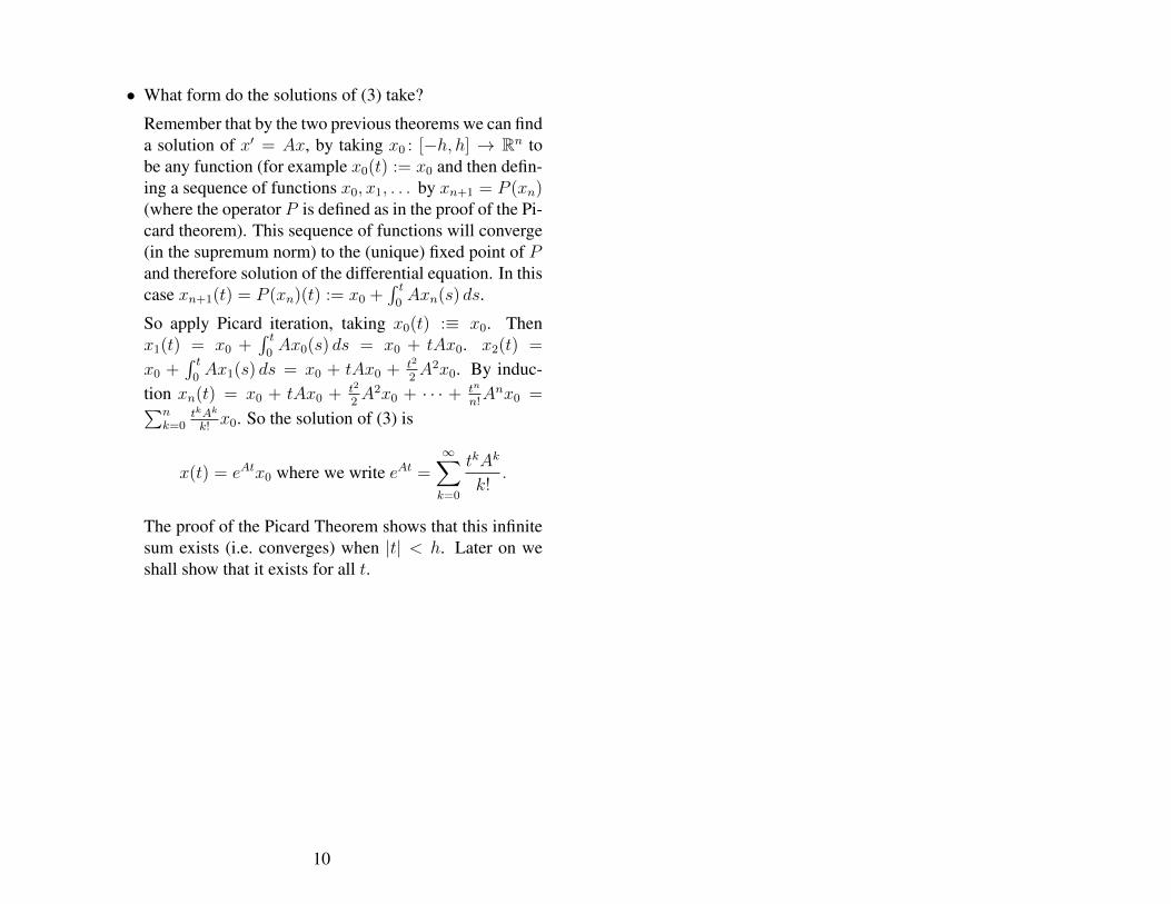
• What form do the solutions of (3) take?

Remember that by the two previous theorems we can finda solution of x′ = Ax, by taking x0 : [−h, h] → Rn tobe any function (for example x0(t) := x0 and then defin-ing a sequence of functions x0, x1, . . . by xn+1 = P (xn)(where the operator P is defined as in the proof of the Pi-card theorem). This sequence of functions will converge(in the supremum norm) to the (unique) fixed point of Pand therefore solution of the differential equation. In thiscase xn+1(t) = P (xn)(t) := x0 +

∫ t0Axn(s) ds.

So apply Picard iteration, taking x0(t) :≡ x0. Thenx1(t) = x0 +

∫ t0Ax0(s) ds = x0 + tAx0. x2(t) =

x0 +∫ t

0Ax1(s) ds = x0 + tAx0 + t2

2A2x0. By induc-

tion xn(t) = x0 + tAx0 + t2

2A2x0 + · · · + tn

n!Anx0 =∑n

k=0tkAk

k!x0. So the solution of (3) is

x(t) = eAtx0 where we write eAt =∞∑

k=0

tkAk

k!.

The proof of the Picard Theorem shows that this infinitesum exists (i.e. converges) when |t| < h. Later on weshall show that it exists for all t.

10

1.9 The Picard Theorem for functions which arelocally Lipschitz

Theorem 3. Picard Theorem (local version). The autonomous version of this theorem goes as follows:Let V ⊂ Rn be open and g : V → Rn continuous, |g| ≤M ,|g(u) − g(v)| ≤ K|u − v|, 0 < h < 1/(2K) and {y; |y −x0)| ≥ hM} ⊂ V . Then there is a unique solution x ∈(−h, h) → Rn of x′ = g(x), x(0) = x0. This follows fromTheorem 3, taking U = R× V and f(t, x) = g(x) on U .

Let U be an open subset of R × Rn containing (0, x0) andassume that

• f : U → Rn is continuous,

• |f | ≤M

• |f(t, u)− f(t, v)| ≤ K|x− y| for all (t, u), (t, v) ∈ U This property we call Locally Lipschitz

• h ∈ (0, 12K

) is chosen so that [−h, h] × {y; |y − x0| ≤hM} ⊂ U (such a choice for h is possible since U open).

dx

dt= f(t, x) and x(0) = x0. (4)

Proof. Fix h > 0 as in the theorem, write I = [−h, h], and letB := {y ∈ Rn; |y − x0| ≤ hM}. Next define C(I, B) as thespace of continuous functions x : I → B ⊂ Rn and

P : C(I, B)→ C(I, B) by P (x)(t) = x0 +

∫ t

0

f(s, x(s)) ds

Then the initial value problem (4) is equivalent to the fixedpoint problem

x = P (x).

We need to show that P is well-defined, i.e. that the expressionP (x)(t) = x0 +

∫ t0f(s, x(s)) ds makes sense, and that when

x ∈ C(I, B) then P (x) ∈ C(I, B). To see this first note thath > 0 is chosen so that when B := {y; |y − x0| ≤ hM} then[−h, h]×B ⊂ U . So

• when x ∈ C(I, B) then f(t, x(t)) is well-defined for allt ∈ [−h, h];

11

• hence x0 +∫ t

0f(s, x(s)) ds is well-defined;

• |f | ≤ M implies [−h, h] 3 t 7→ x0 +∫ t

0f(s, x(s)) ds is

continuous;

• hence t 7→ P (x)(t) is a continuous map;

• finally, |P (x)(t) − x0| ≤∫ h

0|f(s, x(s))| ds ≤ hM . So

P (x)(t) ∈ B for all t ∈ [−h, h] and therefore P (x) ∈C(I, B).

Let us next show that

P : C(I, B)→ C(I, B) by P (x)(t) = x0 +

∫ t

0

f(s, x(s)) ds

is a contraction: for each t ∈ [−h, h],

|P (x)(t)− P (y)(t)| =∣∣∫ t

0(f(s, x(s))− f(t, y(s))) ds

∣∣

≤∫ t

0|f(s, x(s))− f(s, y(s))| ds

≤ K∫ t

0|x(s)− y(s)| ds (Lipschitz)

≤ Ktmax|s|≤t|x(s)− y(s)|

≤ Kh||x− y|| ≤ ||x− y||/2 (since h ∈ (0, 12K

))

Since this holds for all t ∈ [−h, h] we get ||P (x) − P (y)|| ≤||x − y||/2. So P has a unique fixed point, and hence theintegral equation, and therefore the ODE, has a unique solu-tion.

12

1.10 Some comments on the assumptions in Pi-card’s Theorem

• To obtain existence in Theorem 3 it is enough to findsome open set U 3 (0, x0).

• Often one can apply Theorem 3, but not Theorem 2. Takefor example x′ = (1 + x2). Then the r.h.s. is not Lips-chitz on all of R. It is locally Lipschitz though.

• It is not necessary to take the initial time to be t = 0. ThePicard Theorem also gives that there exists h > 0 so thatthe initial value problem

x′ = f(t, x), x(t0) = x0

has a solution (t0 − h, t0 + h) 3 t 7→ x(t) ∈ Rn.

• Let V ⊂ R × Rn and assume that the Jacobian ma- This remark implies that the local Picard Theorem Theorem3 implies a much punchy statement in the most usual settingthat the right hand side of the ODE is continuously differ-entiable: Let f : V → Rn be continuously differentiable.Then for each (0, x0) ∈ U there exists h > 0 and a uniquesolution x : (−h, h)→ Rn of x = f(t, x), x(0) = x0.

trix∂f

∂x(t, x) exists for (t, x) ∈ V and (t, x) 3 V 7→

∂f

∂x(t, x) is continuous. Then for each convex, compact

subset C ⊂ V there exists K ∈ R so that

|f(t, x)− f(t, y)| ≤ K|x− y|.

This follows from the Mean Value Theorem in Rn, seeAppendix A. (So one can apply the previous theorem foreach open set U ⊂ C.)

• If (t, x) 7→ f(t, x) has additional smoothness, the solu-tions will be more smooth. For example, suppose thatf(t, x) is real analytic (i.e. f(t, x) can be written as aconvergent power series), then the solution t 7→ x(t) isalso real analytic.

13

1.11 Some implications of uniqueness in Picard’sTheorem

• If the assumptions of the previous theorem hold and

x1 : I1 → Rn, x2 : I2 → Rn

are both solutions of the initial value problem. Then

x1(t) = x2(t) for all t ∈ I1 ∩ I2.

(See exercises.)

• f : U → Rn does not depend on t (in this case we couldtake U = R× V but in any case f(t, x) = f(0, x) for allt and all x). This case is called autonomous (or time-independent), and so we can write x′ = f(x), x(0) =x0. In this setting solutions cannot cross:

More precisely, if x1, x2 are solutions with x1(t1) = x2(t2) =p ∈ V then

x3(t) = x1(t+ t1) and x4(t) = x2(t+ t2)

are both solutions to x′ = f(x) with x(0) = p. So

x3 ≡ x4.

• The following three important implications for autonomoussystems from local existence uniqueness are explored inAssignment 2 (this material is examinable):

– the existence of a maximal interval (t−, t+) 3 0 ofexistence;

– when t+ <∞ then |x(t)| → ∞ as t→ t+;

– the flow property.

14

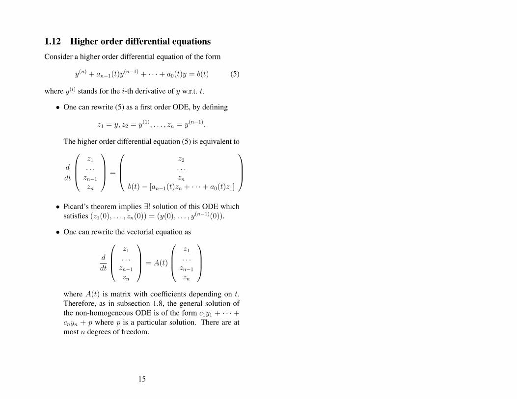
1.12 Higher order differential equationsConsider a higher order differential equation of the form

y(n) + an−1(t)y(n−1) + · · ·+ a0(t)y = b(t) (5)

where y(i) stands for the i-th derivative of y w.r.t. t.

• One can rewrite (5) as a first order ODE, by defining

z1 = y, z2 = y(1), . . . , zn = y(n−1).

The higher order differential equation (5) is equivalent to

d

dt

z1

. . .zn−1

zn

=

z2

. . .zn

b(t)− [an−1(t)zn + · · ·+ a0(t)z1]

• Picard’s theorem implies ∃! solution of this ODE whichsatisfies (z1(0), . . . , zn(0)) = (y(0), . . . , y(n−1)(0)).

• One can rewrite the vectorial equation as

d

dt

z1

. . .zn−1

zn

= A(t)

z1

. . .zn−1

zn

where A(t) is matrix with coefficients depending on t.Therefore, as in subsection 1.8, the general solution ofthe non-homogeneous ODE is of the form c1y1 + · · · +cnyn + p where p is a particular solution. There are atmost n degrees of freedom.

15

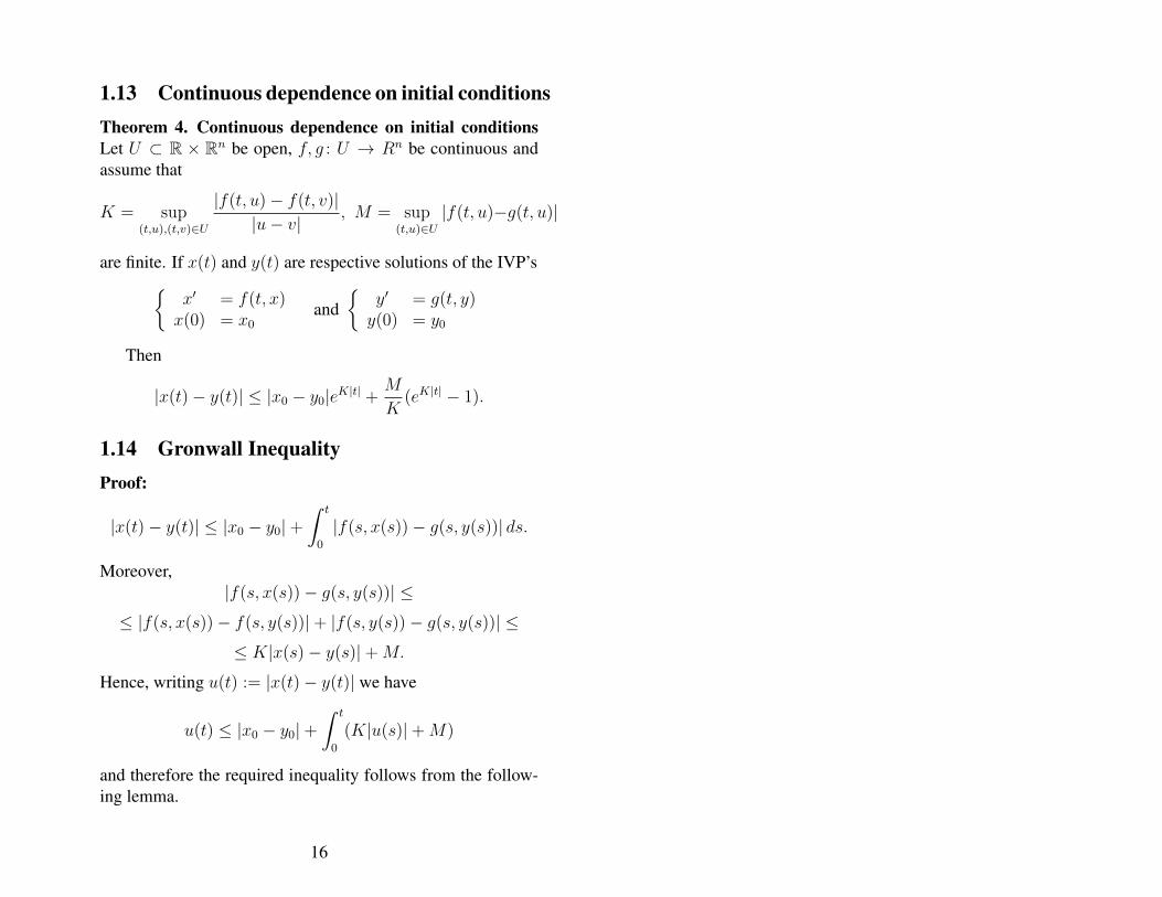
1.13 Continuous dependence on initial conditionsTheorem 4. Continuous dependence on initial conditionsLet U ⊂ R × Rn be open, f, g : U → Rn be continuous andassume that

K = sup(t,u),(t,v)∈U

|f(t, u)− f(t, v)||u− v| , M = sup

(t,u)∈U|f(t, u)−g(t, u)|

are finite. If x(t) and y(t) are respective solutions of the IVP’s{

x′ = f(t, x)x(0) = x0

and{

y′ = g(t, y)y(0) = y0

Then

|x(t)− y(t)| ≤ |x0 − y0|eK|t| +M

K(eK|t| − 1).

1.14 Gronwall InequalityProof:

|x(t)− y(t)| ≤ |x0 − y0|+∫ t

0

|f(s, x(s))− g(s, y(s))| ds.

Moreover,|f(s, x(s))− g(s, y(s))| ≤

≤ |f(s, x(s))− f(s, y(s))|+ |f(s, y(s))− g(s, y(s))| ≤≤ K|x(s)− y(s)|+M.

Hence, writing u(t) := |x(t)− y(t)| we have

u(t) ≤ |x0 − y0|+∫ t

0

(K|u(s)|+M)

and therefore the required inequality follows from the follow-ing lemma.

16

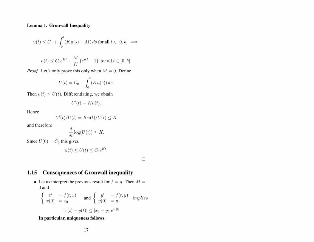
Lemma 1. Gronwall Inequality

u(t) ≤ C0 +

∫ t

0

(Ku(s) +M) ds for all t ∈ [0, h] =⇒

u(t) ≤ C0eKt +

M

K

(eKt − 1

)for all t ∈ [0, h].

Proof. Let’s only prove this only when M = 0. Define

U(t) = C0 +

∫ t

0

(Ku(s)) ds.

Then u(t) ≤ U(t). Differentiating, we obtain

U ′(t) = Ku(t).

HenceU ′(t)/U(t) = Ku(t)/U(t) ≤ K

and therefored

dtlog(U(t)) ≤ K.

Since U(0) = C0 this gives

u(t) ≤ U(t) ≤ C0eKt.

1.15 Consequences of Gronwall inequality• Let us interpret the previous result for f = g. Then M =

0 and{

x′ = f(t, x)x(0) = x0

and{

y′ = f(t, y)y(0) = y0

implies

|x(t)− y(t)| ≤ |x0 − y0|eK|t|.In particular, uniqueness follows.

17

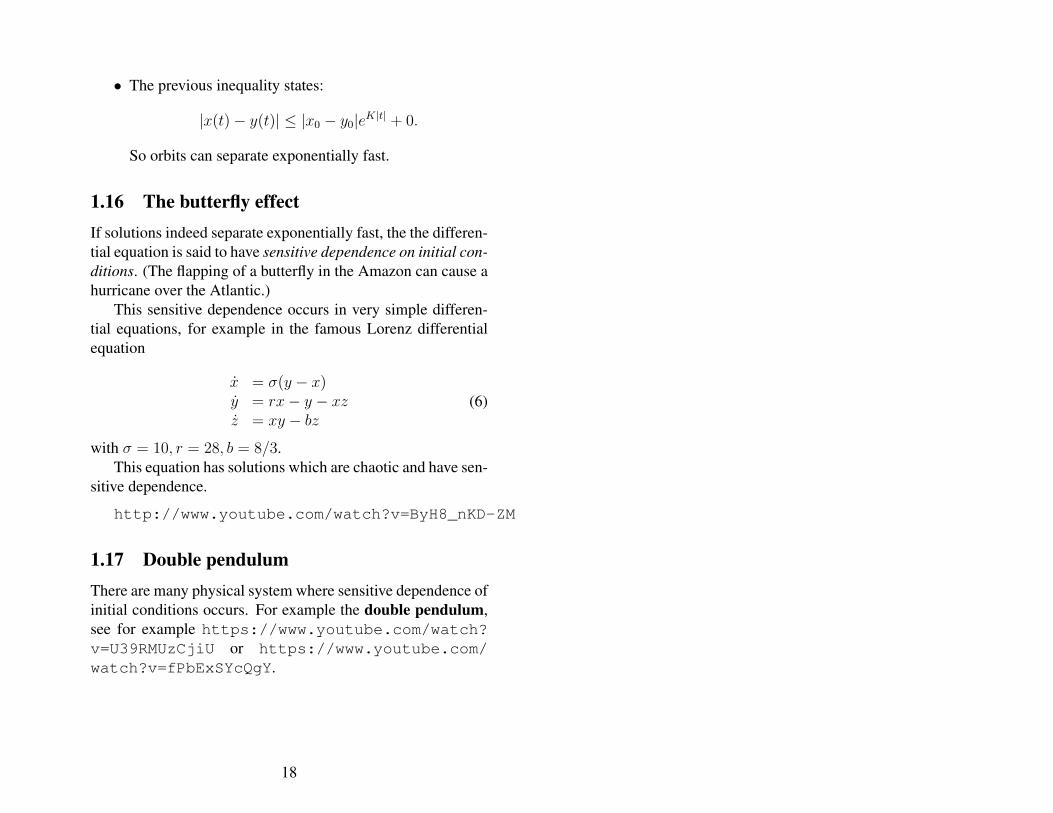
• The previous inequality states:

|x(t)− y(t)| ≤ |x0 − y0|eK|t| + 0.

So orbits can separate exponentially fast.

1.16 The butterfly effectIf solutions indeed separate exponentially fast, the the differen-tial equation is said to have sensitive dependence on initial con-ditions. (The flapping of a butterfly in the Amazon can cause ahurricane over the Atlantic.)

This sensitive dependence occurs in very simple differen-tial equations, for example in the famous Lorenz differentialequation

x = σ(y − x)y = rx− y − xzz = xy − bz

(6)

with σ = 10, r = 28, b = 8/3.This equation has solutions which are chaotic and have sen-

sitive dependence.

http://www.youtube.com/watch?v=ByH8_nKD-ZM

1.17 Double pendulumThere are many physical system where sensitive dependence ofinitial conditions occurs. For example the double pendulum,see for example https://www.youtube.com/watch?v=U39RMUzCjiU or https://www.youtube.com/watch?v=fPbExSYcQgY.

18

2 Linear systems in Rn

In this section we consider

x′ = Ax with x(0) = x0 (7)

where A is a n× n matrix and R 3 t 7→ x(t) ∈ Rn.In Example 1.8 we saw that

etA =∑

k≥0

1

k!(At)k

is defined for |t| small and that x(t) = etAx0 is a solution of(7) for |t| small. In this section we will show that etA is well-defined for all t ∈ R and show how to compute this matrix.

Example 13. Let A =

(λ 00 µ

). Then one has inductively

(tA)k =

((tλ)k 0

0 (tµ)k

). So etA =

(etλ 00 etµ

).

Example 14. Let A =

(λ ε0 λ

). Then one has inductively

(tA)k =

((tλ)k εktkλk−1

0 (tλ)k

). By calculating the infinite

sum of each entry we obtain etA =

(etλ εtetλ

0 etλ

).

Lemma 2. eA is well-defined for any matrix A = (aij).

Proof. let aij(k) be the matrix coefficients of Ak and definea := ||A||∞ := max |aij|. Then

|aij(2)| =∑n

k=1 |aikakj| ≤ na2 ≤ (na)2

|aij(3)| =∑n

k,l |aikaklalj| ≤ n2a3 ≤ (na)3

...|aij(k)| =

∑nk1,k2,...,kn=1 |ak1k2ak2k3 · · · akn−1kn| ≤ nk−1ak ≤ (na)k

19

So∑∞

k=0

|aij(k)|k!

≤ ∑∞k=0

(na)k

k!= exp(na) which means

that the series∑∞

k=0

aij(k)

k!converges absolutely by the com-

parison test. So eA is well-defined.

2.1 Some properties of exp(A)

Lemma 3. Let A,B, T be n × n matrices and T invertible.Then

1. If B = T−1AT then exp(B) = T−1 exp(A)T ;

2. If AB = BA then exp(A+B) = exp(A) exp(B)

3. exp(−A) = (exp(A))−1

Proof. (1) T−1(A+B)T = T−1AT+T−1BT and (T−1AT )k =T−1AkT . Therefore

T−1(n∑

k=0

Ak

k!)T =

n∑

k=0

(T−1AT )k

k!.

(2) follows from the next lemma and (3) follows from (2) tak-ing B = −A.

For general matrices exp(A+B) 6= exp(A) exp(B).

Note that if AB = BA then (A + B)n = n!∑

j+k=n

Aj

j!

Bk

k!.

So (2) in the previous lemma follows from:

Lemma 4.∞∑

n=0

∑

j+k=n

Aj

j!

Bk

k!=∞∑

j=0

Aj

j!

∞∑

k=0

Bk

k!.

20

Proof: A computation shows

2m∑

n=0

∑

j+k=n

Aj

j!

Bk

k!−

m∑

j=0

Aj

j!

m∑

k=0

Bk

k!=

′∑ Aj

j!

Bk

k!+

′′∑ Aj

j!

Bk

k!

where∑′ respectively

∑′′ denote the sum over terms

j + k ≤ 2m, 0 ≤ j ≤ m,m+ 1 ≤ k ≤ 2m,

j + k ≤ 2m,m+ 1 ≤ j ≤ 2m, 0 ≤ k ≤ m.

So the absolutely values of the coefficients in∑′ Aj

j!

Bk

k!are

bounded by∑m

j=0

||Aj||∞j!

∑2mk=m+1

||Bk||∞k!

. As in the proof

Lemma 2 the latter term goes to zero as m→∞.

Similarly∑′′ Aj

j!

Bk

k!goes to zero as→∞. This completes

the proof of Lemma 4.

Example 15.

exp

(a b−b a

)=

(eat cos(bt) eat sin(bt)−eat sin(bt) eat cos(bt)

).

This is proved in the first assignment of week 3 and also inSection 2.4.

Each coefficient of etA depends on t. So defined

dtetA to be

the matrix obtained by differentiating each coefficient.

Lemma 5.d

dtexp(tA) = A exp(tA) = exp(tA)A.

21

40 Chapter 3 Phase Portraits for Planar Systems

with !1 < 0 < !2. This can be solved immediately since the system decouplesinto two unrelated first-order equations:

x ! = !1x

y ! = !2y .

We already know how to solve these equations, but, having in mind whatcomes later, let’s find the eigenvalues and eigenvectors. The characteristicequation is

(! " !1)(! " !2) = 0

so !1 and !2 are the eigenvalues. An eigenvector corresponding to !1 is (1, 0)and to !2 is (0, 1). Hence we find the general solution

X(t ) = "e!1t!

1

0

"+ #e!2t

!0

1

".

Since !1 < 0, the straight-line solutions of the form "e!1t (1, 0) lie on thex-axis and tend to (0, 0) as t # $. This axis is called the stable line. Since!2 > 0, the solutions #e!2t (0, 1) lie on the y-axis and tend away from (0, 0) ast # $; this axis is the unstable line. All other solutions (with ", # %= 0) tendto $ in the direction of the unstable line, as t # $, since X(t ) comes closerand closer to (0, #e!2t ) as t increases. In backward time, these solutions tendto $ in the direction of the stable line. !

In Figure 3.1 we have plotted the phase portrait of this system. The phaseportrait is a picture of a collection of representative solution curves of the

Figure 3.1 Saddle phaseportrait for x ! = –x,y ! = y.

3.1 Real Distinct Eigenvalues 43

(a) (b)

Figure 3.3 Phase portraits for (a) a sink and(b) a source.

Since !1 < !2 < 0, we call !1 the stronger eigenvalue and !2 the weakereigenvalue. The reason for this in this particular case is that the x-coordinates ofsolutions tend to 0 much more quickly than the y-coordinates. This accountsfor why solutions (except those on the line corresponding to the !1 eigen-vector) tend to “hug” the straight-line solution corresponding to the weakereigenvalue as they approach the origin.

The phase portrait for this system is displayed in Figure 3.3a. In this case theequilibrium point is called a sink.

More generally, if the system has eigenvalues !1 < !2 < 0 with eigenvectors(u1, u2) and (v1, v2), respectively, then the general solution is

"e!1t!

u1u2

"+ #e!2t

!v1v2

".

The slope of this solution is given by

dy

dx= !1"e!1t u2 + !2#e!2t v2

!1"e!1t u1 + !2#e!2t v1

=!

!1"e!1t u2 + !2#e!2t v2

!1"e!1t u1 + !2#e!2t v1

"e!!2t

e!!2t

= !1"e(!1!!2)t u2 + !2#v2

!1"e(!1!!2)t u1 + !2#v1,

which tends to the slope v2/v1 of the !2 eigenvector, unless we have # = 0. If# = 0, our solution is the straight-line solution corresponding to the eigen-value !1. Hence all solutions (except those on the straight line corresponding

Proof.

d

dtexp(tA) = lim

h→0

exp((t+ h)A)− exp(tA)

h=

= limh→0

exp(tA) exp(hA)− exp(tA)

h=

= exp(tA) limh→0

exp(hA)− Ih

= exp(tA)A.

Here the last equality follows from the definition of exp(hA) =

I + hA+h2

2!A2 + . . . .

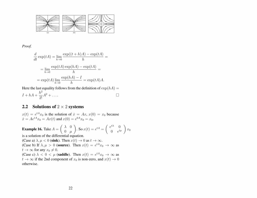
2.2 Solutions of 2× 2 systemsx(t) = etAx0 is the solution of x = Ax, x(0) = x0 becausex = AetAx0 = Ax(t) and x(0) = e0Ax0 = x0.

Example 16. TakeA =

(λ 00 µ

). So x(t) = etA =

(etλ 00 etµ

)x0

is a solution of the differential equation.(Case a) λ, µ < 0 (sink). Then x(t)→ 0 as t→∞.(Case b) If λ, µ > 0 (source). Then x(t) = etAx0 → ∞ ast→∞ for any x0 6= 0.(Case c) λ < 0 < µ (saddle). Then x(t) = etAx0 → ∞ ast → ∞ if the 2nd component of x0 is non-zero, and x(t) → 0otherwise.

22

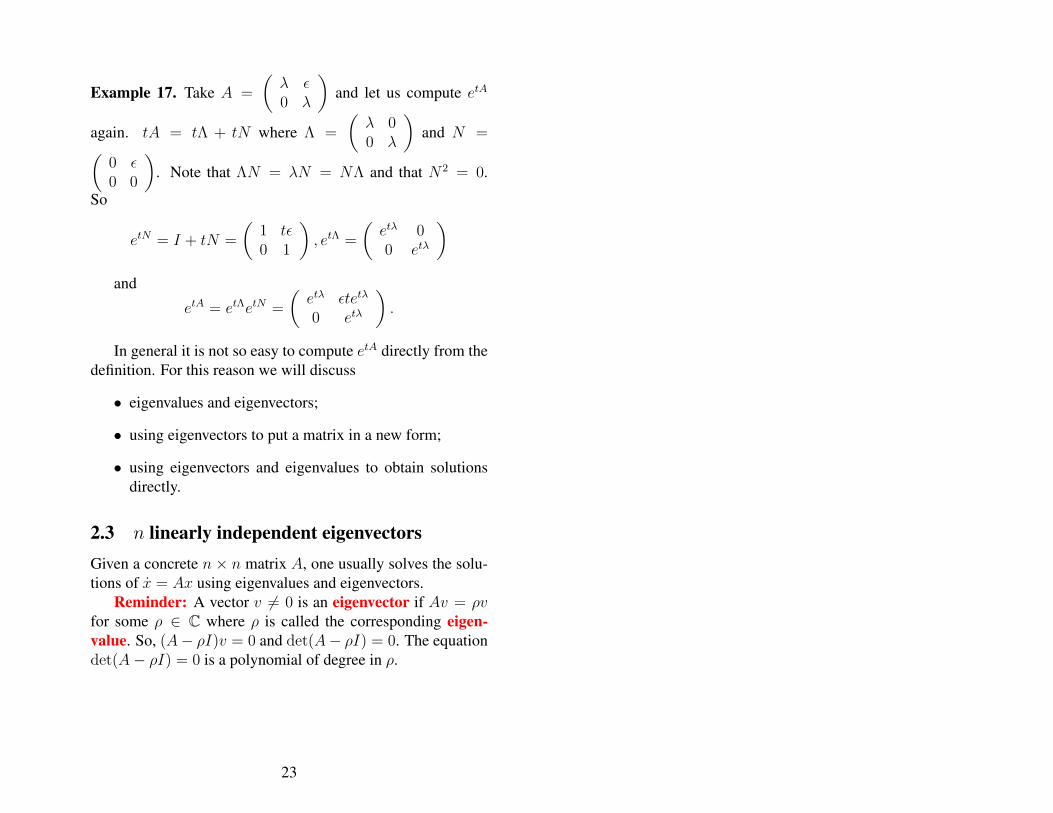
Example 17. Take A =

(λ ε0 λ

)and let us compute etA

again. tA = tΛ + tN where Λ =

(λ 00 λ

)and N =

(0 ε0 0

). Note that ΛN = λN = NΛ and that N2 = 0.

So

etN = I + tN =

(1 tε0 1

), etΛ =

(etλ 00 etλ

)

and

etA = etΛetN =

(etλ εtetλ

0 etλ

).

In general it is not so easy to compute etA directly from thedefinition. For this reason we will discuss

• eigenvalues and eigenvectors;

• using eigenvectors to put a matrix in a new form;

• using eigenvectors and eigenvalues to obtain solutionsdirectly.

2.3 n linearly independent eigenvectorsGiven a concrete n × n matrix A, one usually solves the solu-tions of x = Ax using eigenvalues and eigenvectors.

Reminder: A vector v 6= 0 is an eigenvector if Av = ρvfor some ρ ∈ C where ρ is called the corresponding eigen-value. So, (A− ρI)v = 0 and det(A− ρI) = 0. The equationdet(A− ρI) = 0 is a polynomial of degree in ρ.

23

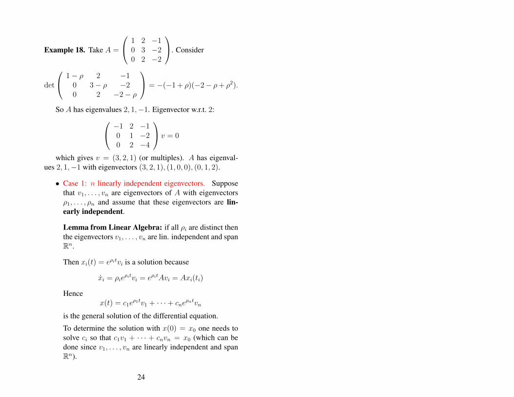
Example 18. Take A =

1 2 −10 3 −20 2 −2

. Consider

det

1− ρ 2 −10 3− ρ −20 2 −2− ρ

= −(−1 + ρ)(−2− ρ+ ρ2).

So A has eigenvalues 2, 1,−1. Eigenvector w.r.t. 2:−1 2 −10 1 −20 2 −4

v = 0

which gives v = (3, 2, 1) (or multiples). A has eigenval-ues 2, 1,−1 with eigenvectors (3, 2, 1), (1, 0, 0), (0, 1, 2).

• Case 1: n linearly independent eigenvectors. Supposethat v1, . . . , vn are eigenvectors of A with eigenvectorsρ1, . . . , ρn and assume that these eigenvectors are lin-early independent.

Lemma from Linear Algebra: if all ρi are distinct thenthe eigenvectors v1, . . . , vn are lin. independent and spanRn.

Then xi(t) = eρitvi is a solution because

xi = ρieρitvi = eρitAvi = Axi(ti)

Hencex(t) = c1e

ρ1tv1 + · · ·+ cneρntvn

is the general solution of the differential equation.

To determine the solution with x(0) = x0 one needs tosolve ci so that c1v1 + · · · + cnvn = x0 (which can bedone since v1, . . . , vn are linearly independent and spanRn).

24

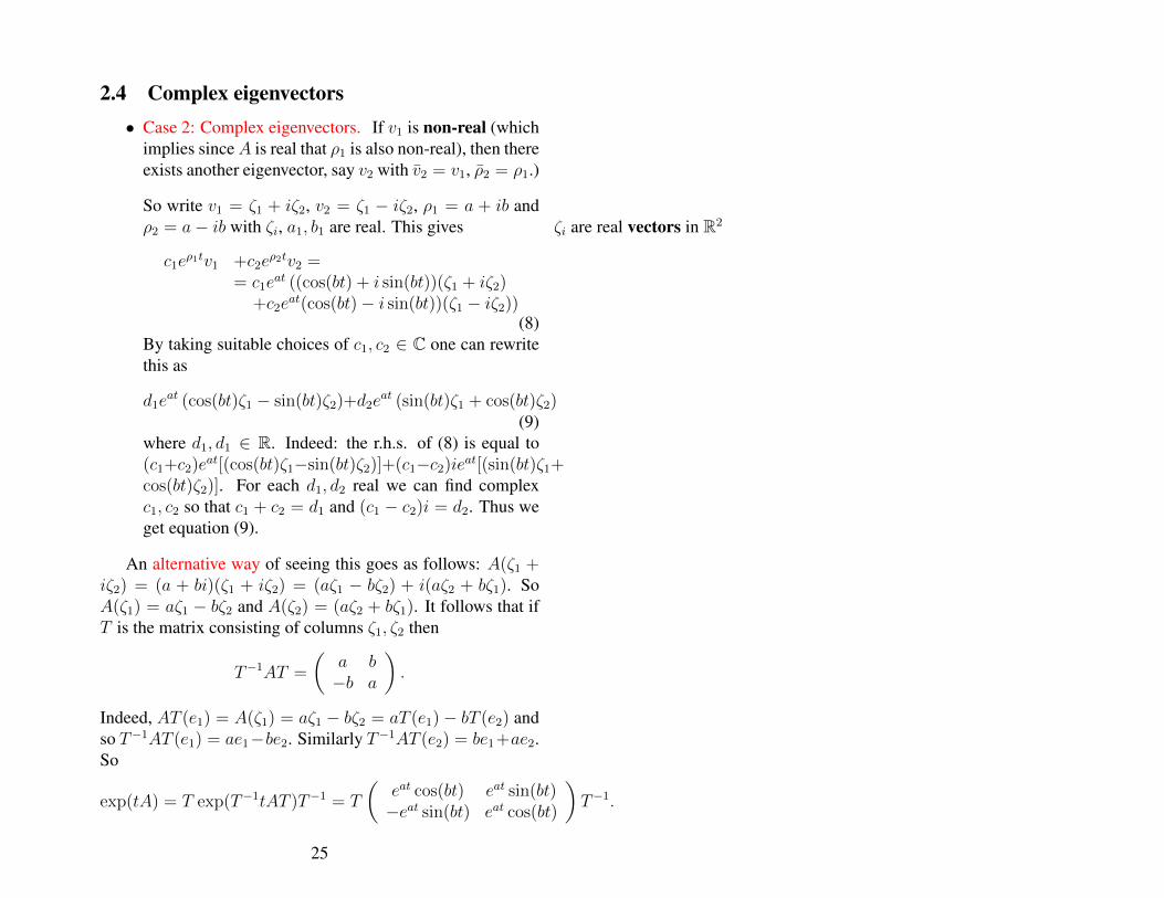
2.4 Complex eigenvectors• Case 2: Complex eigenvectors. If v1 is non-real (which

implies sinceA is real that ρ1 is also non-real), then thereexists another eigenvector, say v2 with v2 = v1, ρ2 = ρ1.)

So write v1 = ζ1 + iζ2, v2 = ζ1 − iζ2, ρ1 = a + ib andρ2 = a− ib with ζi, a1, b1 are real. This gives ζi are real vectors in R2

c1eρ1tv1 +c2e

ρ2tv2 == c1e

at ((cos(bt) + i sin(bt))(ζ1 + iζ2)+c2e

at(cos(bt)− i sin(bt))(ζ1 − iζ2))(8)

By taking suitable choices of c1, c2 ∈ C one can rewritethis as

d1eat (cos(bt)ζ1 − sin(bt)ζ2)+d2e

at (sin(bt)ζ1 + cos(bt)ζ2)(9)

where d1, d1 ∈ R. Indeed: the r.h.s. of (8) is equal to(c1+c2)eat[(cos(bt)ζ1−sin(bt)ζ2)]+(c1−c2)ieat[(sin(bt)ζ1+cos(bt)ζ2)]. For each d1, d2 real we can find complexc1, c2 so that c1 + c2 = d1 and (c1 − c2)i = d2. Thus weget equation (9).

An alternative way of seeing this goes as follows: A(ζ1 +iζ2) = (a + bi)(ζ1 + iζ2) = (aζ1 − bζ2) + i(aζ2 + bζ1). SoA(ζ1) = aζ1 − bζ2 and A(ζ2) = (aζ2 + bζ1). It follows that ifT is the matrix consisting of columns ζ1, ζ2 then

T−1AT =

(a b−b a

).

Indeed, AT (e1) = A(ζ1) = aζ1 − bζ2 = aT (e1)− bT (e2) andso T−1AT (e1) = ae1−be2. Similarly T−1AT (e2) = be1 +ae2.So

exp(tA) = T exp(T−1tAT )T−1 = T

(eat cos(bt) eat sin(bt)−eat sin(bt) eat cos(bt)

)T−1.

25

Here we use Example 15. Now write(d1

d2

)= Tx0 and

check that

exp(At)x0 = T

(eat cos(bt) eat sin(bt)−eat sin(bt) eat cos(bt)

)(d1

d2

)=

d1eat (cos(bt)ζ1 − sin(bt)ζ2) + d2e

at (sin(bt)ζ1 + cos(bt)ζ2) .

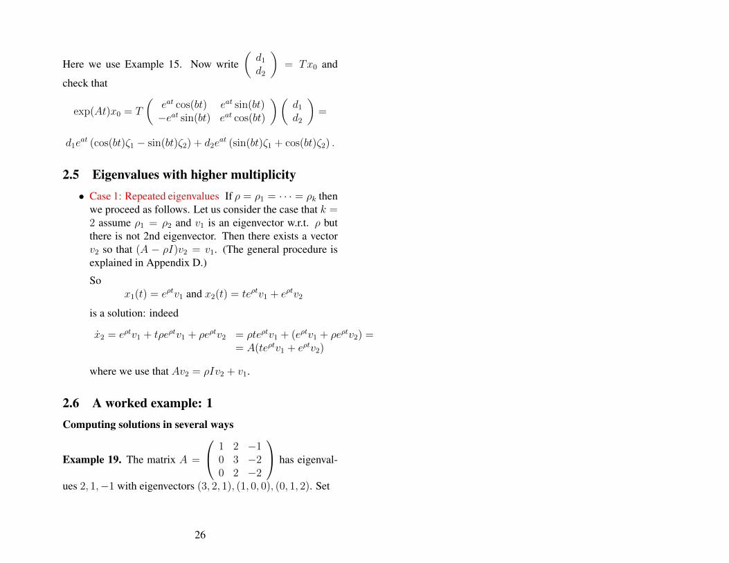
2.5 Eigenvalues with higher multiplicity• Case 1: Repeated eigenvalues If ρ = ρ1 = · · · = ρk then

we proceed as follows. Let us consider the case that k =2 assume ρ1 = ρ2 and v1 is an eigenvector w.r.t. ρ butthere is not 2nd eigenvector. Then there exists a vectorv2 so that (A − ρI)v2 = v1. (The general procedure isexplained in Appendix D.)

Sox1(t) = eρtv1 and x2(t) = teρtv1 + eρtv2

is a solution: indeed

x2 = eρtv1 + tρeρtv1 + ρeρtv2 = ρteρtv1 + (eρtv1 + ρeρtv2) == A(teρtv1 + eρtv2)

where we use that Av2 = ρIv2 + v1.

2.6 A worked example: 1Computing solutions in several ways

Example 19. The matrix A =

1 2 −10 3 −20 2 −2

has eigenval-

ues 2, 1,−1 with eigenvectors (3, 2, 1), (1, 0, 0), (0, 1, 2). Set

26

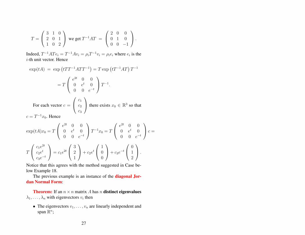
T =

3 1 02 0 11 0 2

we get T−1AT =

2 0 00 1 00 0 −1

.

Indeed, T−1ATei = T−1Avi = ρiT−1vi = ρiei where ei is the

i-th unit vector. Hence

exp(tA) = exp(tTT−1ATT−1

)= T exp

(tT−1AT

)T−1

= T

e2t 0 00 et 00 0 e−t

T−1.

For each vector c =

c1

c2

c3

there exists x0 ∈ R3 so that

c = T−1x0. Hence

exp(tA)x0 = T

e2t 0 00 et 00 0 e−t

T−1x0 = T

e2t 0 00 et 00 0 e−t

c =

T

c1e2t

c2et

c3e−t

= c1e

2t

321

+ c2e

t

100

+ c3e

−t

012

.

Notice that this agrees with the method suggested in Case be-low Example 18.

The previous example is an instance of the diagonal Jor-dan Normal Form:

Theorem: If an n×n matrix A has n distinct eigenvaluesλ1, . . . , λn with eigenvectors vi then

• The eigenvectors v1, . . . , vn are linearly independent andspan Rn;

27

• If we take T the matrix with columns v1, . . . , vn then

T−1AT =

λ1 0. . .

0 λn

.

• etA = T

etλ1 0. . .

0 etλn

T−1.

2.7 A second worked exampleIn the example below, we explain what to do when there isno basis of eigenvectors. As you will see, the example alsoexplains what to do in the general situation.

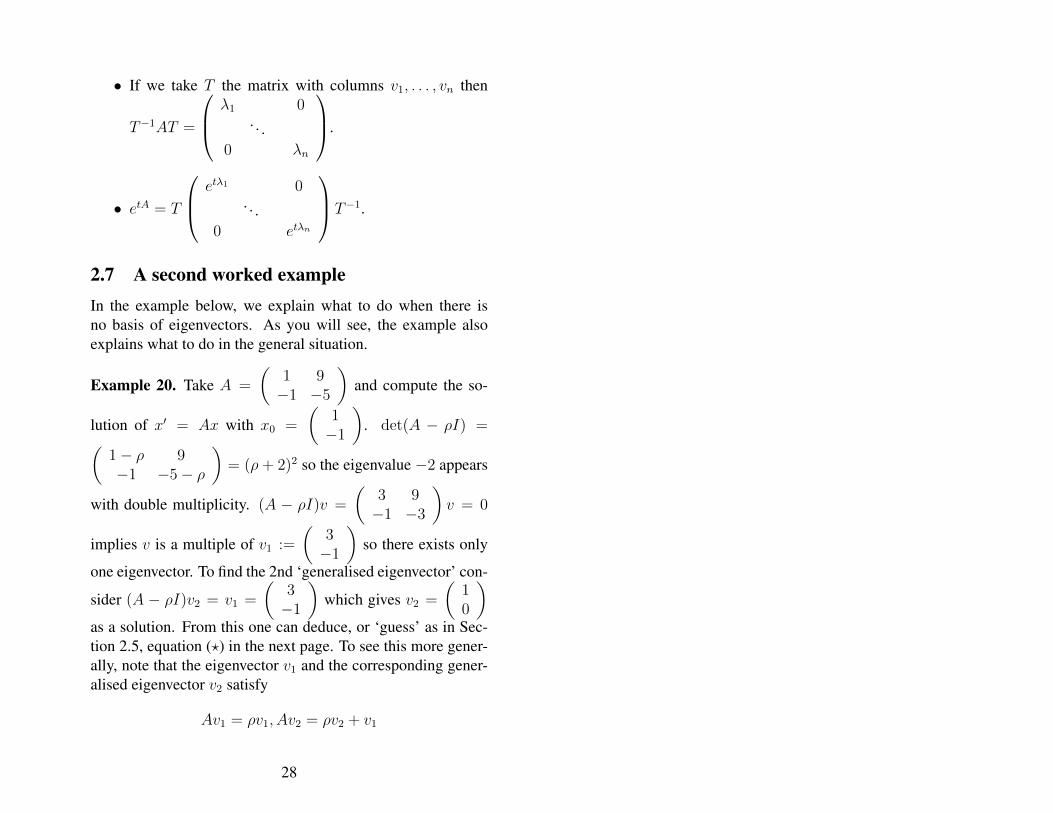
Example 20. Take A =

(1 9−1 −5

)and compute the so-

lution of x′ = Ax with x0 =

(1−1

). det(A − ρI) =

(1− ρ 9−1 −5− ρ

)= (ρ+ 2)2 so the eigenvalue −2 appears

with double multiplicity. (A − ρI)v =

(3 9−1 −3

)v = 0

implies v is a multiple of v1 :=

(3−1

)so there exists only

one eigenvector. To find the 2nd ‘generalised eigenvector’ con-

sider (A − ρI)v2 = v1 =

(3−1

)which gives v2 =

(10

)

as a solution. From this one can deduce, or ‘guess’ as in Sec-tion 2.5, equation (?) in the next page. To see this more gener-ally, note that the eigenvector v1 and the corresponding gener-alised eigenvector v2 satisfy

Av1 = ρv1, Av2 = ρv2 + v1

28

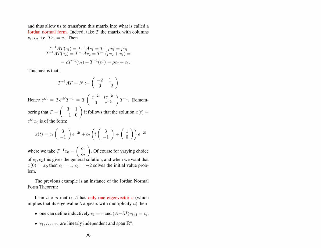
and thus allow us to transform this matrix into what is called aJordan normal form. Indeed, take T the matrix with columnsv1, v2, i.e. Tei = vi. Then

T−1AT (e1) = T−1Av1 = T−1ρv1 = ρe1

T−1AT (e2) = T−1Av2 = T−1(ρv2 + v1) =

= ρT−1(v2) + T−1(v1) = ρe2 + e1.

This means that:

T−1AT = N :=

(−2 10 −2

)

Hence etA = TetNT−1 = T

(e−2t te−2t

0 e−2t

)T−1. Remem-

bering that T =

(3 1−1 0

)it follows that the solution x(t) =

etAx0 is of the form:

x(t) = c1

(3−1

)e−2t + c2

(t

(3−1

)+

(10

))e−2t

where we take T−1x0 =

(c1

c2

). Of course for varying choice

of c1, c2 this gives the general solution, and when we want thatx(0) = x0 then c1 = 1, c2 = −2 solves the initial value prob-lem.

The previous example is an instance of the Jordan NormalForm Theorem:

If an n × n matrix A has only one eigenvector v (whichimplies that its eigenvalue λ appears with multiplicity n) then

• one can define inductively v1 = v and (A−λI)vi+1 = vi.

• v1, . . . , vn are linearly independent and span Rn.

29

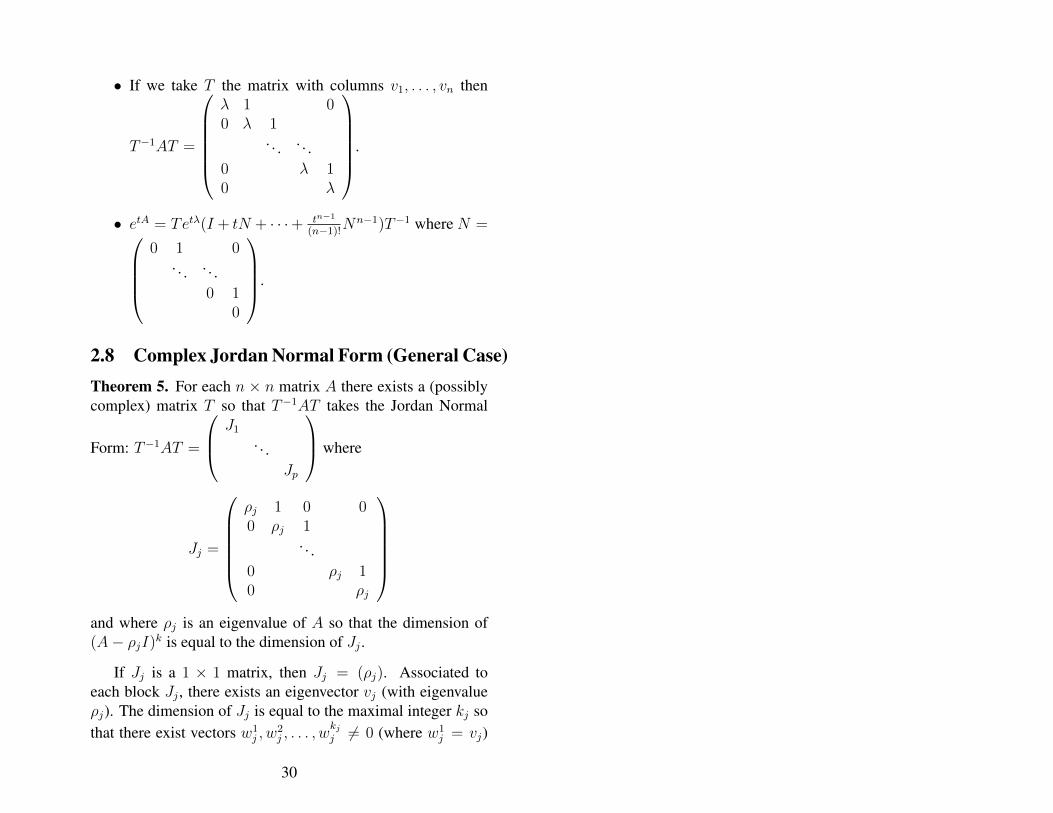
• If we take T the matrix with columns v1, . . . , vn then

T−1AT =

λ 1 00 λ 1

. . . . . .0 λ 10 λ

.

• etA = Tetλ(I + tN + · · ·+ tn−1

(n−1)!Nn−1)T−1 where N =

0 1 0. . . . . .

0 10

.

2.8 Complex Jordan Normal Form (General Case)Theorem 5. For each n × n matrix A there exists a (possiblycomplex) matrix T so that T−1AT takes the Jordan Normal

Form: T−1AT =

J1

. . .Jp

where

Jj =

ρj 1 0 00 ρj 1

. . .0 ρj 10 ρj

and where ρj is an eigenvalue of A so that the dimension of(A− ρjI)k is equal to the dimension of Jj .

If Jj is a 1 × 1 matrix, then Jj = (ρj). Associated toeach block Jj , there exists an eigenvector vj (with eigenvalueρj). The dimension of Jj is equal to the maximal integer kj sothat there exist vectors w1

j , w2j , . . . , w

kjj 6= 0 (where w1

j = vj)

30

inductively defined as (A− ρjI)wi+1j = wij for i = 1, . . . , kj −

1. The matrix T has columns w11, . . . , w

k11 , . . . , w

1p, . . . , w

kpp .

In the computations above, we showed how to determine Tso this holds.

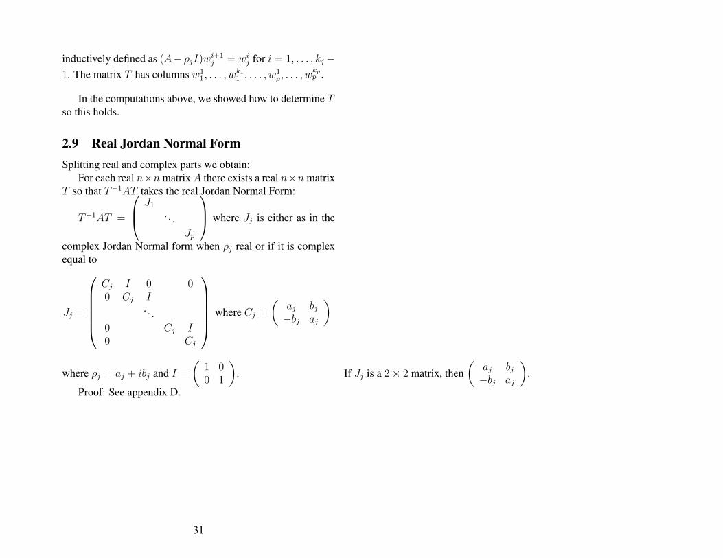
2.9 Real Jordan Normal FormSplitting real and complex parts we obtain:

For each real n×nmatrixA there exists a real n×nmatrixT so that T−1AT takes the real Jordan Normal Form:

T−1AT =

J1

. . .Jp

where Jj is either as in the

complex Jordan Normal form when ρj real or if it is complexequal to

Jj =

Cj I 0 00 Cj I

. . .0 Cj I0 Cj

where Cj =

(aj bj−bj aj

)

where ρj = aj + ibj and I =

(1 00 1

). If Jj is a 2× 2 matrix, then

(aj bj−bj aj

).

Proof: See appendix D.

31

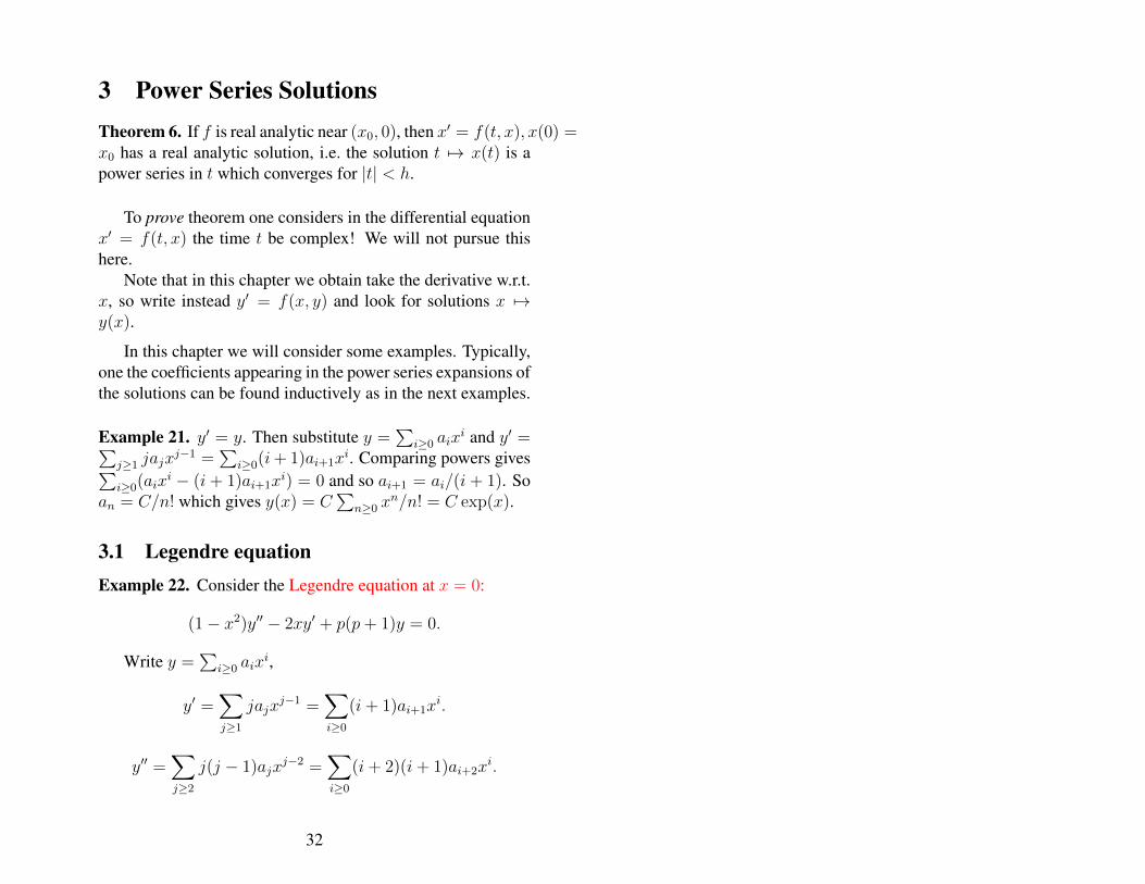
3 Power Series SolutionsTheorem 6. If f is real analytic near (x0, 0), then x′ = f(t, x), x(0) =x0 has a real analytic solution, i.e. the solution t 7→ x(t) is apower series in t which converges for |t| < h.

To prove theorem one considers in the differential equationx′ = f(t, x) the time t be complex! We will not pursue thishere.

Note that in this chapter we obtain take the derivative w.r.t.x, so write instead y′ = f(x, y) and look for solutions x 7→y(x).

In this chapter we will consider some examples. Typically,one the coefficients appearing in the power series expansions ofthe solutions can be found inductively as in the next examples.

Example 21. y′ = y. Then substitute y =∑

i≥0 aixi and y′ =∑

j≥1 jajxj−1 =

∑i≥0(i+ 1)ai+1x

i. Comparing powers gives∑i≥0(aix

i − (i + 1)ai+1xi) = 0 and so ai+1 = ai/(i + 1). So

an = C/n! which gives y(x) = C∑

n≥0 xn/n! = C exp(x).

3.1 Legendre equationExample 22. Consider the Legendre equation at x = 0:

(1− x2)y′′ − 2xy′ + p(p+ 1)y = 0.

Write y =∑

i≥0 aixi,

y′ =∑

j≥1

jajxj−1 =

∑

i≥0

(i+ 1)ai+1xi.

y′′ =∑

j≥2

j(j − 1)ajxj−2 =

∑

i≥0

(i+ 2)(i+ 1)ai+2xi.

32

We determine ai as follows.

y′′ − x2y′′ − 2xy′ + p(p+ 1)y =

∑

i≥0

(i+2)(i+1)ai+2xi−∑

i≥2

i(i−1)aixi−2

∑

i≥1

iaixi+p(p+1)

∑

i≥0

aixi

=∑

i≥2

[(i+ 2)(i+ 1)ai+2 − i(i− 1)ai − 2iai + p(p+ 1)ai]xi+

+(2a2 + 6xa3)− 2a1x+ p(p+ 1)(a0 + a1x)

∑

i≥0

(i+2)(i+1)ai+2xi−∑

i≥2

i(i−1)aixi−2

∑

i≥1

iaixi+p(p+1)

∑

i≥0

aixi

=∑

i≥2

[(i+ 2)(i+ 1)ai+2 − i(i− 1)ai − 2iai + p(p+ 1)ai]xi+

+(2a2 + 6xa3)− 2a1x+ p(p+ 1)(a0 + a1x)

So collecting terms with the same power of x together givesa2 = −p(p+1)

2a0 and a3 = (2−p(p+1))

6a1 and

ai+2 =[i(i− 1) + 2i− p(p+ 1)]ai

(i+ 1)(i+ 2)= −(p− i)(p+ i+ 1)

(i+ 2)(i+ 1)ai.

If p is an integer, ap+2j = 0 for j ≥ 0. Convergence ofy =

∑i≥0 aix

i for |x| < 1 follows from the ratio test.

3.2 Second order equations with singular pointsSometimes one encounters a differential equation where thesolutions are not analytic because the equation has a pole. Forexample

y′′ + (1/x)y′ − (1/x2)y = 0.

33

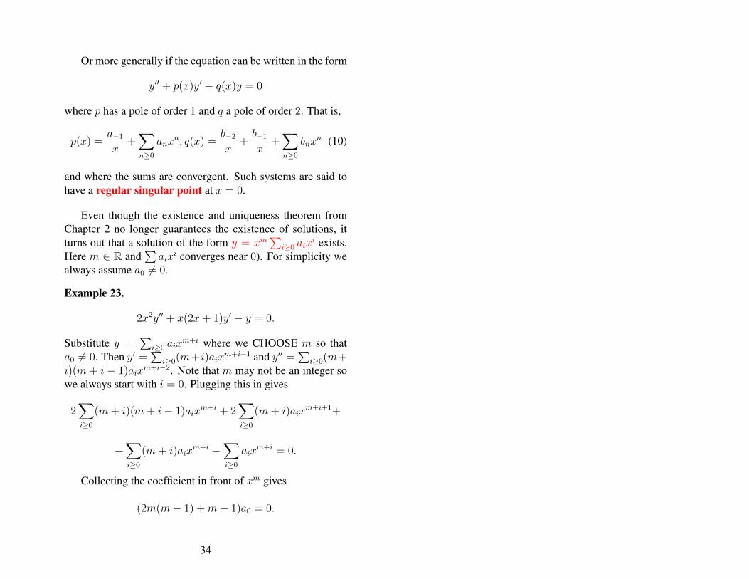
Or more generally if the equation can be written in the form

y′′ + p(x)y′ − q(x)y = 0

where p has a pole of order 1 and q a pole of order 2. That is,

p(x) =a−1

x+∑

n≥0

anxn, q(x) =

b−2

x+b−1

x+∑

n≥0

bnxn (10)

and where the sums are convergent. Such systems are said tohave a regular singular point at x = 0.

Even though the existence and uniqueness theorem fromChapter 2 no longer guarantees the existence of solutions, itturns out that a solution of the form y = xm

∑i≥0 aix

i exists.Here m ∈ R and

∑aix

i converges near 0). For simplicity wealways assume a0 6= 0.

Example 23.

2x2y′′ + x(2x+ 1)y′ − y = 0.

Substitute y =∑

i≥0 aixm+i where we CHOOSE m so that

a0 6= 0. Then y′ =∑

i≥0(m+ i)aixm+i−1 and y′′ =

∑i≥0(m+

i)(m + i − 1)aixm+i−2. Note that m may not be an integer so

we always start with i = 0. Plugging this in gives

2∑

i≥0

(m+ i)(m+ i− 1)aixm+i + 2

∑

i≥0

(m+ i)aixm+i+1+

+∑

i≥0

(m+ i)aixm+i −

∑

i≥0

aixm+i = 0.

Collecting the coefficient in front of xm gives

(2m(m− 1) +m− 1)a0 = 0.

34

Since we assume a0 6= 0 we get the equation 2m(m−1)+m−1 = 0 which gives m = −1/2, 1. The coefficient in front of allthe terms with xm+i gives

2(m+i)(m+i−1)ai+2(m+i−1)ai−1+(m+i)ai−ai = 0, i.e.

[2(m+ i)(m+ i− 1) + (m+ i)− 1]ai = −2(m+ i− 1)ai−1.

If m = −1/2 this gives aj =3− 2j

−3j + 2j2aj−1.

If m = 1 then this gives aj =−2j

3j + 2j2aj−1.

So y = Ax−1/2 (1− x+ (1/2)x2 + . . . )+Bx (1− (2/5)x+ . . . ).The ratio test gives that (1− x+ (1/2)x2 + . . . ) and (1− (2/5)x+ . . . )converge for all x ∈ R.

Remark: The equation required to have the lowest orderterm vanish is called the indicial equation which has two rootsm1,m2 (possibly of double multiplicity).

Theorem 7. Consider a differential equation y′′ + p(x)y′ −q(x)y = 0 where p, q are as in equation (10). Then

• If m1−m2 is not an integer than we obtain two indepen-dent solutions of the form y1(x) = xm1

∑i≥0 aix

i andy2(x) = xm2

∑i≥0 aix

i.

• Ifm1−m2 is an integer than one either can find a 2nd so-lution in the above form, or - if that fails - a 2nd solutionof the form log(x)y1(x) where y1(x) is the first solution.

Certain families of this kind of differential equation withregular singular points, appear frequently in mathematical physics.

• Legendre equation

y′′ − 2x

1− x2y′ +

p(p+ 1)

1− x2y = 0

35

• Bessel equation

x2y′′ + xy′ + (x2 − p2)y = 0

• Gauss’ Hypergeometric equation

x(1− x)y′′ + [c− (a+ b+ 1)x]y′ − aby = 0

For suitable choices of a, b solutions of this are the sine,cosine, arctan and log functions.

3.3 Computing invariant sets by power seriesOne can often obtain curves through certain points as conver-gent power series.

Example 24. Let x′ = x+ y2, y′ = −y + x2.

• This is an autonomous differential equation in the plane.

• Solutions are unique (r.h.s. is locally Lipschitz).

• So solutions are of the form t 7→ φt(x, y) where φt(x, y)has the flow property φt+s(x, y) = φtφs(x, y).

• Of course at φt(0, 0) = (0, 0) for all t, since the r.h.s. ofthe differential equation is zero (the speed is zero there).

• Nevertheless we can find a curve γ of the form y = ψ(x)with the property that if (x, y) ∈ γ then φt(x, y) ∈ γ for typo correctedall t (for which φt(x, y) exists).

• Later on we shall see that x′ = x + y2, y′ = −y + x2

locally behaves very much like the equation in which thehigher order terms are removed: x′ = x, y′ = −y. Forthis linear equation the x-axis (y = 0) is invariant: onthat line we have x′ = −x and so orbits go to 0 in thelinear case.

36

• What about the non-linear case? Let us assume that onecan write y as a function of x, i.e. y = ψ(x). Then since,x′ = x+ y2, y′ = −y + x2 we have

ψ′(x) = (dy

dt)/(

dx

dt) =−y + x2

x+ y2=−ψ(x) + x2

x+ [ψ(x)]2.

Let us assume 0 ∈ γ and write y = ψ(x) = a1x+a2x2 +

a3x3 + . . . . Comparing terms gives

a1+2a2x+3a3x2+· · · = −[a1x+ a2x

2 + a3x3 + . . . ] + x2

x+ [a1x+ a2x2 + a3x3 + . . . ]2.

Comparing terms of the same power, shows that a1 = 0,2a2 = (1− a2− a2

1) and so on. This gives a curve whichis tangent to the x-axis so that orbits remain in this curve.

37

4 Boundary Value Problems, Sturm-LiouvilleProblems and Oscillatory equations

Instead of initial conditions, in this chapter we will considerboundary values. Examples:

• y′′+y = 0, y(0) = 0, y(π) = 0. This has infinitely manysolutions: y(x) = c sin(x).

• y′′ + y = 0, y(0) = 0, y(π) = ε 6= 0 has no solutions:y(x) = a cos(x) + b sin(x) and y(0) = 0 implies a = 0and y(π) = 0 has no solutions.

• Clearly boundary problems are more subtle.

• We will concentrate on equations of the form u′′+λu = 0with boundary conditions, where λ is a free parameter.

• This class of problems is relevant for a large class ofphysical problems: heat, wave and Schroedinger equa-tions.

• This generalizes Fourier expansions.

4.1 Motivation: wave equationConsider the wave equation:

∂2

∂t2u(x, t) =

∂2

∂x2u(x, t)

where x ∈ [0, π] and the end points are fixed:

u(0, t) = 0, u(π, t) = 0 for all t ,

Below we shall see that some additional condition is neededon f to ensure that one can find a solution u which is C2.These technical conditions are not examinable.

u(x, 0) = f(x),∂

∂tu(x, t)|t=0 = 0.

38

• This is a model for a string of length π on a musicalinstrument such as a guitar; before the string is releasedthe shape of the string is f(x).

• As usual one solves this by writing u(x, t) = w(x) ·v(t),substituting this into the wave equation and then obtain-ing w′′(x)/w(x) = v′′(t)/v(t). Since the left hand doesnot depend on t and the right hand side not on x thisexpression is equal to some constant λ and we get

w′′ = λw and v′′ = λv.

• We need to set w(0) = w(π) = 0 to satisfy the boundaryconditions that u(0, t) = u(π, t) = 0 for all t.

Write λ = −µ2 where µ is not necessarily real.

• When λ 6= 0, v′′ = λv has solution

v(t) = c1 cos(µt) + c2 sin(µt).

• Consider w′′ − λw = 0 and w(0) = w(π) = 0.

– λ = 0 implies w(x) = c3 + c4x and because of theboundary condition c3 = c4 = 0. So can assumeλ 6= 0.

– If λ 6= 0, solution isw(x) = c3 cos(µx)+c4 sin(µx).w(0) = 0 =⇒ c3 = 0

therefore w(π) = c4 sin(µπ) = 0 implies µ = n ∈N[check: µ is non-real =⇒ sin(µπ) 6= 0]. So

w(x) = c4 sin(nx) and λ = −n2 and n ∈ N \ {0}.

39

• So for any n ∈ N we obtain solution

u(x, t) = w(x)v(t) = (c1 cos(nt) + c2 sin(nt)) sin(nx).

• The string can only vibrate with frequencies which are amultiple of N.

So u(x, t) =∑

n≥1(c1,n cos(nt) + c2,n sin(nt)) sin(nx) issolution provided the sum makes sense and is twice differen-tiable.

Lemma 6.∑n2|c1,n| < ∞ and

∑n2|c2,n| < ∞ =⇒

u(x, t) =∑

n≥1(c1,n cos(nt) + c2,n sin(nt)) sin(nx) is C2.Note that in these notes, lemmas and theorems are num-bered separately. So Theorem 8 follows Theorem 7 notLemma 7.

Proof. That∑N

n=1(c1,n cos(nt)+c2,n sin(nt)) sin(nx) convergesfollows from

Weierstrass test: ifMn ≥ 0,∑Mn <∞ and un : [a, b]→

R is continuous with supx∈[a,b] |un(x)| ≤ Mn then∑un con-

verges uniformly on [a, b] (and so the limit is continuous too!).Since the d/dx derivative of

N∑

n=1

(c1,n cos(nt) + c2,n sin(nt)) sin(nx)

is equal to∑N

n=1(c1,n cos(nt)+ c2,n sin(nt))n cos(nx), and thelatter converges, u(x, t) is differentiable w.r.t. x.

Next we need to make sure that the boundary conditions aresatisfied. The first boundary condition is

∂

∂tu(x, t)|t=0 = 0 for all x ∈ [0, π] (11)

This implies that∑c2,nn sin(nx) ≡ 0 =⇒ c2,n = 0 for all

n ≥ 0. So we obtain that a solution is of the form

u(x, t) =∞∑

n=1

c1,n cos(nt) sin(nx).

40

The second boundary condition is

u(x, 0) =∑

c1,n sin(nx) = f(x) for all x ∈ [0, π]. (12)

This looks like a Fourier expansion, as in Theorem 8. The rea- Note that if f : [0, π] → R and f(0) = f(π) = 0 then wecan define the function g : [0, 2π]→ R so that g(x) = f(x)for x ∈ [0, π] and g(x) = f(2π − x) for x ∈ [π, 2π].It follows that g(π − x) = −g(π + x) for x ∈ [0, π].So this means that

∫ 2π

0g(x) cos(nx) dx = 0 and there-

fore in the Fourier expansion of g the cosine terms van-ish, and we have g(x) =

∑∞n=1 s1,n sin(nx). In particular

f(x) =∑∞

n=1 s1,n sin(nx).

son why it is possible to do this so that only the sin terms appearis explained in the margin. Note that we we to make sure thatu(x, 0) =

∑c1,n sin(nx) = f(x) holds uniformly, and that in

fact u(x, t) is C2. To make sure of this, we need to apply The-orem 9 and assume that f is C3 and f(0) = f(π) = f ′′(0) =f ′′(π) = 0 the assumptions in Lemma 6 are satisfied. For anexplanation why these conditions on f implies n2|c1,n| < ∞,see the proof of Theorem 10 below.

The following theorem is quite straightforward:

Theorem 8. L2 Fourier Theorem. If f : [0, 2π] → R is con-tinuous (or continuous except at a finite number of points) thenwe one can coefficients c1,n, c2,n so that

f ∼∞∑

n=0

(c1,n cos(nx) + c2,n sin(nx))

in the sense that∫ 2π

0

|f(x)−N∑

n=0

(c1,n cos(nx) + c2,n sin(nx))|2 dx→ 0

as N →∞.

What we need here is a uniform convergence:

Theorem 9. Fourier Theorem with uniform convergence. As-sume f : [0, π] → R is C2 (twice continuously differentiable)and f(0) = f(π) = 0 then one can find s1,n so that

N∑

n=1

s1,n sin(nx) converges uniformly to f(x) as N →∞.

41

We will not prove this theorem here, but elaborate some ofthe ideas in the sketch of the proof of the next theorem (whichis not examinable).

Theorem 10. If f is C3 and f(0) = f(π) = f ′′(0) = f ′′(π) =0, then the assumptions in Lemma 6 are satisfied.

Proof. (Non examinable). Let us assume that f is C2, f(0) =f(π) = 0. According to the previous theorem (the FourierTheorem) one can therefore write f(x) =

∑n≥1 sn sin(nx).

Let us now show that if f is C3 and f(0) = f(π) = f ′′(0) =f ′′(π) = 0 the assumptions in Lemma 6 are satisfied, i.e. thatf and f ′ can be written in the form f(x) =

∑sn(f ′) sin(nx)

and f ′(x) =∑cn(f ′) cos(nx) and that

∑n2s2

n < ∞ and∑n2c2

n < ∞. Let us prove that∑ |sn| < ∞. (We change the clarified the logic here a bit

notation from the coefficients cn to sn in the main text sincethe new notation is more natural here.) This remark and theproof below are not examinable, and will given in sketchyform only. First choose constants sn(f) and cn(f ′) so thatf(x) =

∑sn(f) sin(nx) and f ′(x) =

∑cn(f ′) cos(nx) (by

the Fourier theorem one can write f ′ in this way since is C2

and since f ′′(0) = f ′′(π) = 0). Step 1:

(f ′, f ′) =∑

n,m≥0

cn(f ′)cm(f ′)

∫ π

0

cos(nx) cos(mx) =

= (π/2)∑

n≥1

|cn(f ′)|2 + π|c0|2.

It follows that∑

n≥0 |cn(f ′)|2 < ∞. Step 2: for n ≥ 1 wehave

sn(f) = (2/π)

∫ π

0

f(x) sin(nx) dx

andcn(f ′) = (2/π)

∫ π

0

f ′(x) sin(nx) dx.

42

Using partial integration on the last expression, and using thatf(0) = f(π) = 0 gives for n ≥ 1,

cn(f ′) = (2/π)

∫ π

0

f ′(x) cos(nx) dx = (2/π)[f(x) cos(nx)]π0 +

+n(2/π)

∫ 1

0

f(x) sin(nx) dx = (2n/π)sn(f).

It follows from this, f(0) = f(π) = 0 and Step 1 that∑n2|sn(f)|2 <

∞. Step 3: Now we use the Cauchy inequality∑anbn ≤∑

a2n

∑b2n. Taking an = 1/n and bn = n|sn(f)| we get that∑ |sn(f)| =

∑anbn ≤

∑a2n

∑b2n. By Step 2,

∑b2n < ∞

and since∑

1/n2 <∞, it follows that∑ |sn(f)| <∞. In the

same way, we can prove that if f is C3 and f(0) = f(π) =f ′(0) = f ′(π) = f ′′(0) = f ′′(π) = 0 then

∑n2|sn(f)| <

∞. Therefore the assumptions in Lemma 6 are satisfied. Ifwe assume f(0) = f(π) = f ′′(0) = f ′′(π) = 0 and con-sider g(x) = f(x) − a1 sinx − a2 sin 2x with a1, a2 so thatg′(0) = g′(π) = 0 then we can apply the above to g. It followsthat

∑n2|sn(g)| < ∞. This also implies

∑n2|sn(f)| < ∞.

This concludes the explanation of item 2 above Theorem 9.

In conclusion we get:

• Provided we assume that f(0) = f(π) = f ′′(0) = f ′′(π)and that f is C3 we can find

u(x, t) =∞∑

n=1

c1,n cos(nt) sin(nx)

which is C2 and solves the wave equation together withthe boundary conditions.

• c1,n can be found by methods you have seen before.

• Since w′′ = λw, one calls λ an eigenvalue and w aneigenfunction.

43

4.2 A typical Sturm-Liouville ProblemIn this subsection we will state the Sturm-Liouville Theoremwhich generalises the previous Fourier theorem.

Let us consider another example:

y′′ + λy = 0, y(0) + y′(0) = 0, y(1) = 0.

• If λ = 0 then y(x) = c1 + c2x and the boundary condi-tions give y(x) = 1− x.

• If λ 6= 0 we write again λ = µ2. The equation y′′+λy =0 gives y(x) = c1e

iµx + c2e−iµx.

• Plugging in y(0) + y′(0) = 0, y(1) = 0 gives

• (c1 + c2) + iµ(c1 − c2) = 0 and c1eiµ + c2e

−iµ = 0.Indeed, 0 = (1 + iµ)(cosµ − i sinµ) − (1 − iµ)(cosµ +i sinµ) = (2(µ cosµ − sinµ), so tanµ = µ. The easi-est way to show that this has only real roots, is by usingthat eigenvalues are real, see Subsection 4.3. One can provethis also by elementary methods, but this is much more in-volved. For example, take µ = s + it with s, t real. Thenyou (1 + iµ)e−iµ − (1 − iµ)eiµ = 0 can be rewritten as

e2is(cos 2t + i sin 2t) =1 + is− t1− is+ t

and do some geometric

calculations...

• So c2 = −c1e2iµ and (1 + iµ)e−iµ − (1 − iµ)eiµ = 0.

tanµ = µ (see margin). This has infinitely many so-lutions µn ∈ [0,∞), n = 0, 1, . . . with µn → ∞ andµn ≈ (2n+ 1)π/2.

• Eigenvalues: λn = µ2n ≈ (2n + 1)2(π/2)2, n = 0, . . . ;

eigenfunctions: y0(x) = 1−x and yn(x) = sin(√λn(1−

x)), n ≥ 1. To see this, note that we have y(x) =[c1e

iµx + c2e−iµx] = c1[eiµx− e2iµe−iµx] = c1[e−iµ+iµx−

eiµ−iµx] = 2c1 sin(µx − µ). Here c1 is a new (complex)constant. So yn(x) = sin(µn(1− x) is an eigenfunction.

44

These are special cases of following type of problem: givenfunctions p, q, r : [a, b]→ R find y : [a, b]→ R so that

(p(x)y′)′ + q(x)y + λr(x)y = 0. (13)

Theorem 11. Sturm-Louiville Theorem Assume that p, r >0 are continuous and p is C1 on [a, b]. Then (13) with theboundary conditions (14)

α0y(a) + α1y′(a) = 0, β0y(b) + β1y

′(b) = 0. (14)

(where αi, βi are assumed to be real and neither of the vectors(α0, α1), (β0, β1) are allowed to be zero) has infinitely manysolutions with the following properties:

1. The eigenvalues λn are real, distinct and of single multi-plicity;

2. The eigenvalues λn tend to infinity, so λ1 < λ2 < . . .and λn →∞.

3. If n 6= m then corresponding eigenfunctions yn, ym areorthogonal in the sense that

∫ b

a

ym(x)yn(x)r(x) dx = 0.

In other words, one can find coefficients cn, n = 0, 1, 2, . . .so that f is the limit of the sequence of functions

∑Nn=0 cnyn.

More precisely, if f is merely continuous than this con-vergence is in the L2 sense, while if f is C2 then thisconvergence is uniform (this sentence is not examinable,and in this course we will not cover a proof of this sen-tence).

4. Each continuous function can be expanded in terms ofthe eigenfunctions, as in the Fourier case!!

45

Let’s make two additional remarks:

• Note that if yn, ym are solutions and we set

W (ym, yn)(x) := det(ym(x) y′m(x)yn(x) y′n(x)

) = ym(x)y′n(x)−yn(x)y′m(x)

then W (a) = 0 and W (b) = 0. To see this, note that thefirst boundary condition in equation (14) implies

(ym(a) y′m(a)yn(a) y′n(a)

)(α0

α1

)= 0.

Since (α0, α1) 6= (0, 0) the determinant of the matrix iszero.

• How to find an so that f(x) =∑

n≥0 anyn(x)? Just take

(f, ryk) = (∑

n≥0 anyn(x), ryk) =∑

n≥0 an(yn, ryk)= ak(yk, ryk).

Here we used in the last equality that (yn, ryk) 6= 0 im-plies n = k. Hence

ak :=(f, ryk)

(yk, ryk)

where (v, w) is the inner product: (v, w) =∫ bav(t)w(t) dt.

4.3 A glimpse into symmetric operators• Sturm-Liouville problems are solved using some opera-

tor theory: the 2nd order differential equation is equiva-lent to

Ly(x) = λr(x)y(x) where L =

(− d

dxp(x)

d

dx− q(x)

).

This turns out to be a symmetric operator in the sensethat (Lv,w) = (v, Lw) where (v, w) =

∫ bav(x)w(x) dx

is as defined above.

46

• The situation for analogous to the finite dimensional case:

• L is a symmetric (and satisfies some additional proper-ties) =⇒ its eigenvalues are real, and its eigenfunctionsform a basis.

L is symmetric (self-adjoint) on the space of functionssatisfying the boundary conditions. Let Lu = −(pu′)′ − quand Lv = −(pv′)′ − qv.∫ baL(u)v dx =

∫ ba[−(pu′)′v − quv] dx.

∫ bauL(v) dx =∫ b

a[−u(pv′)′ − quv] dx.

∫ ba−(pu′)′v dx = −pu′v|ba +

∫ bapu′v′ dx

= −pu′v|ba + puv′|ba −∫ bau(pv′)′ dx.

Hence

∫ ba[L(u)v− uL(v)] dx = −p(x)[u′v − uv′]

∣∣∣b

a

= − [p(b)W (u, v)(b)− p(a)W (u, v)(a)]

If u, v satisfy the boundary conditions, then α0u(a)+α1u′(a) =

0 and α0v(a) + α1v′(a) = 0. Since α0, α1 are real, therefore

α0v(a) + α1v′(a) = 0. Hence, W (u, v)(a) = W (u, v)(b) = 0,

and therefore∫ b

a

[L(u)v − uL(v)] dx = 0.

In other words, L is self-adjoint is on the space H of func-tions satisfying the boundary conditions. That is,

∫ b

a

[L(u)v − uL(v)] dx = 0, i.e. (Lu, v) = (u, Lv).

47

Proof that eigenvalues are real and orthogonality of eigen-functions: Define (u, v) =

∫ bau(x)v(x) dx. Then the para-

graph showed (Lu, v) = (u, Lv).

• Suppose that Ly = rλy. Then the eigenvalue λ is real:Indeed,

λ(ry, y) = (λry, y) = (Ly, y) = (y, Ly) = λ(y, ry) = λ(ry, y)

since r is real. Since (ry, y) > 0 it follows that λ = λ.

• Suppose that Ly = rλy and Lz = rµz.

λ 6= µ =⇒∫ bar(x)y(x)z(x) dx = (ry, z) = 0.

So the eigenfunctions y, z are orthogonal. Indeed,

λ(ry, z) = (λry, z) = (Ly, z) = (y, Lz) = (y, µrz)= µ(y, rz) = µ(ry, z) = µ(ry, z).

where we have used that r and µ are real. Since λ 6= µ itfollows that (ry, z) = 0.

Remark 1. In this remark (which is not examinable) we dis-cuss what is required for the proof of the above theorem:

• to define Hilbert space H: this is a Banach space withan inner product for which (v, w) = (w, v) where z iscomplex conjugation;

• to define the norm ||v|| =√

(v, v) (generalizing ||z|| = typo corrected√

(z, z) =√zz on C); Note ||v|| =

√∫ ba|v(x)|2 dx, the

so-called L2 norm.

• to associate to a linear A : H → H the operator norm||A|| = supf∈H,||f ||=1 ||Af ||;

48

• to call a linear operator A is compact if for each se-quence ||fn|| ≤ 1, there exists a convergent subsequenceof Afn.

• to show that ifA : H → H is compact, then there exists asequence of eigenvalues αn → 0 and eigenfunctions un.These eigenvalues are all real and the eigenfunctions areorthogonal. If the closure of A(H) is equal to H , thenfor each f ∈ H then one can write f =

∑∞j=0(uj, f)uj .

• The operator L in Sturm-Liouville problems is not com-pact, and that is why one considers some related operator(the resolvent).

• This related operator is compact.

• The above theorem then follows.

The Sturm-Liouville Theorem is fundamental in

• quantum mechanics;

• in large range of boundary value problems;

• and related to geometric problems describing propertiesof geodesics.

4.4 Oscillatory equationsConsider (py′)′ + ry = 0 where p > 0 and C1 as before.

Theorem 12. Let y1, y2 be solutions. Then the Wronskian x 7→W (y1, y2)(x) := y1(x)y′2(x)− y2(x)y′1(x) has constant sign.

49

Proof. (py′1)′ + ry1 = 0 and (py′2)′ + ry2 = 0. Multiplying thefirst equation by y2 and the second one by y1 and subtract:

0 = y2(py′1)′ − y1(py′2)′ = y2p′y′1 + y2py

′′1 − y1p

′y′2 − y1py′′2 .

Differentiating W and substituting the last equation in

pW ′ = p[y′1y′2 + y1y

′′2 − y′2y′1 − y2y

′′1 ] = py1y

′′2 − py2y

′′1

givespW ′ = −p′W.

This implies that ifW (x) = 0 for some x ∈ [a, b] thenW (x) =0 for all x ∈ [a, b].

Lemma 7. W (y1, y2) ≡ 0 =⇒ ∃c ∈ R with y1 = cy2 (ory2 = 0).

Proof. Since W (y1, y2) = 0, y2 6= 0 implies (y1, y′1) is a mul-

tiple of (y2, y′2). Can this multiple depend on x? No: if

y1(x) = c(x)y2(x) and y′1(x) = c(x)y′2(x) ∀x=⇒ c(x)y′2(x) = y′1(x) = c′(x)y2(x) + c(x)y′2(x) ∀x.

Hence c′ ≡ 0.

Theorem 13. Sturm Separation Theorem Let y1, y2 be two so-lutions which are independent (one is not a constant multipleof the other). Then zeros are interlaced: between consecutivezeros of y1 there is a zero of y2 and vice versa.

Proof. Assume y1(a) = y1(b) = 0. y′1(a) 6= 0 (otherwisey1 ≡ 0) and y′2(b) 6= 0. We may choose a, b so that y1(x) > 0for x ∈ (a, b). Then y′1(a)y′1(b) < 0. (Draw a picture.) Also,

W (y1, y2)(a) = −y2(a)y′1(a) and W (y1, y2)(b) = −y2(b)y′1(b).

Since y′1(a)y′1(b) < 0 and W (a)W (b) > 0 (W does not changesign), we get y2(a)y2(b) < 0, which implies that y2 has a zerobetween a and b.

50

5 Calculus of VariationsMany problems result in differential equations. In this chapterwe will consider the situation where these arise from a min-imisation (variational) problem. Specifically, the problems wewill consider are of the type

• Minimize

I[y] =

∫ 1

0

f(x, y(x), y′(x)) dx (15)

where f is some function and y is an unknown function.

• Minimize (15) conditional to some restriction of the typeJ [y] =

∫ 1

0f(x, y(x), y′(x)) dx = 1.

5.1 Examples (the problems we will solve in thischapter):

Example 25. Let A = (0, 0) and B = (1, 0) with l, b > 0and consider a path of the form [0, 1] 37→ c(t) = (c1(t), c2(t)),connecting A and B. What is the shortest path?

Task: Choose [0, 1] 3 t 7→ c(t) = (c1(t), c2(t)) with c(0) =(0, 0) and c(1) = (1, 0) which minimises

L[c] =

∫ 1

0

√c′1(t)2 + c′2(t)2 dt.

Of course this is a line segment, but how to make this pre-cise?

If we are not in a plane, but in a surface or a higher dimen-sional set, these shortest curves are called geodesics, and theseare studied extensively in mathematics.

Example 26. Let A = (0, 0) and B = (l,−b) with l, b > 0 andconsider a path of the form (x, y(x)), x ∈ [0, l], connecting

51

A and B. Take a ball starting at A and rolling along this pathunder the influence of gravity to B. Let T be the time this ballwill take. Which function x 7→ y(x) which will minimise T ?

The sum of kinetic and potential energy is constant

(1/2)mv2 +mgh = const.

Since the ball rolls along (x, y(x)) we have v(x) =√−2gy(x).

Let s(t) be the length travelled at time t. Then v = ds/dt.Hence dt = ds/v or

T [y] :=

∫ l

0

√1 + y′(x)2

√−2gy(x)

dx.

Task: minimise T [y] within the space of functions x 7→y(x) for which y and y′ continuous and y(0) = 0 and y(l) =−b. This is called the Brachisotochrome, going back to Bernouilliin 1696.

Example 27. Take a closed curve in the plane without self-intersections and of length one. What is the curve c whichmaximises the area D it encloses? Again, let [0, 1] 37→ c(t) =(c1(t), c2(t)) with c(0) = c(1) and so that s, t ∈ [0, 1) ands 6= t implies c(s) 6= c(t).

The length of the curve is againL[c] =∫ 1

0

√c′1(t)2 + c′2(t)2 dt.

To compute the area of D we use the Green theorem:∫

c

Pdx+Qdy =

∫ ∫

D

(∂Q

∂x− ∂P

∂y)dxdy

Take P ≡ 0 and Q = x. Then

∫ ∫

D

(∂Q

∂x− ∂P

∂y)dxdy =

∫ ∫

D

1 dxdy = area of D.

So

A[c] =

∫ ∫

D

1 dxdy =

∫

c

xdy =

∫ 1

0

c1(t)c′2(t) dt.

52

This is an isoperimetric problem: find the supremum ofA[c] given L[c] = 1.

5.2 Extrema in the finite dimensional caseWe say that F : Rn → R take a local minimum at x if thereexists δ > 0 so that

F (x) ≥ F (x) for all x with |x− x| < δ.

Theorem 14. Assume that F is differentiable at a and also hasa minimum at x then DF (x) = 0.

Proof. Let us first assume that n = 1. Then that f has a min-imum means that F (x + h) − F (x) ≥ 0 for all h near zero.Hence

F (x+ h)− F (x)

h≥ 0 for h > 0 near zero and

F (x+ h)− F (x)

h≤ 0 for h < 0 near zero.

Therefore

F ′(x) = limh→0

F (x+ h)− F (x)

h= 0

Let us consider the case that n > 1 and reduce to the casethat n = 1. So take a vector v at x, define l(t) = x + tv andg(t) := F ◦ l(t). So we can use the first part of the proof andthus we get g′(0) = 0. Applying the chain rule 0 = g′(0) =Dg(0) = DF (l(0))Dl(0) = DF (x)v and so

∂F

∂x1

(x)v1 + · · ·+ ∂F

∂xn(x)vn = 0.

Hence DF (x)v = 0 where DF (x) is the Jacobian matrix at x.Since this holds for all v, we get DF (x) = 0.

53

Remember we also wrote sometimes DFx for the matrixDF (x) and that DF (x)v is the directional derivative of f at xin the direction v.

5.3 The Euler-Lagrange equationThe infinite dimensional case: the Euler-Lagrange equation

• In the infinite dimensional case, we will take F : H → Rwhere H is some function space. The purpose of thischapter is to generalise the previous result to this setting,and show that the solutions of this problem gives rise todifferential equations.

• Mostly the function space is the space C1[a, b] of C1

functions y : [a, b] → Rn. This space is an infinite di-mensional vector space (in fact, a Banach space) withnorm |y|C1 = supx∈[a,b](|y(x)|, |Dy(x)|).

• Choose some function f : [a, b] × Rn × Rn → R. Take(x, y, y′) ∈ [a, b]×Rn×Rn denote by fy, fy′ the corre-sponding partial derivatives. So fy(x, y, y′) and fy′(x, y, y′)vectors. Attention: here y and y′ are just the names ofvectors in Rn (and not - yet - functions or derivatives offunctions).

• Here fy is the part of the 1×(1+n+n) vectorDf whichconcerns the y derivatives.

Assume f : [a, b] × Rn × Rn → R with fy, fy′ continuousand define I : C1[a, b]→ R by,

I[y] =

∫ b

a

f(x, y(x), y′(x)) dx.

Given y : [a, b]→ Rn, let’s denote

fy[y](x) = fy(x, y(x), y′(x)) and fy′ [y](x) = fy′(x, y(x), y′(x))

54

where fy, fy′ are the corresponding partial derivatives of f . Fixya, yb ∈ Rn and define

A = {y; y : [a, b]→ Rn is C1 and y(a) = ya, y(b) = yb}.

Theorem 15. If A 3 y 7→ I[y] has a minimum at y then

1. for every v ∈ C1[a, b] with v(a) = v(b) = 0 we get∫ ba(fy[y] · v + fy′ [y]v′) dx = 0.

2. fy′ [y] exists, is continuous on [a, b] and

d

dxfy′ [y] = fy[y].

Proof. Remember that

A = {y; y : [a, b]→ Rn is C1 and y(a) = ya, y(b) = yb}.

Hence v ∈ C1[a, b] with v(a) = v(b) = 0, then y+hv ∈ A foreach h. So the space A is affine.

Assume that I : C1[a, b] → R has a minimum at y, whichmeans that

I[y + hv] ≥ I[y] ∀v ∈ C1[a, b], v(a) = v(b) = 0 ∀h ∈ R

I[y + hv]− I[y] =

=

∫ b

a

f(x, (y + hv)(x), (y + hv)′(x))− f(x, y(x), y′(x))dx.

By Taylor’s Theorem,

f(x, (y + hv)(x), (y + hv)′(x))− f(x, y(x), y′(x)) =

fy[y]hv + fy′ [y]hv′ + o(h).

So

I[y + hv]− I[y] = h ·[∫ b

a

[fy[y]v + fy′ [y]v′] dx

]+ o(h).

55

Hence a necessary condition for y to be a minimum of I is∫ b

a

[fy[y]v + fy′ [y]v′] dx = 0

for each v ∈ C1[a, b] with v(a) = v(b) = 0.Partial integration gives∫ b

a

fy′ [y]v′ dx = (fy′ [y]v)∣∣ba−∫ b

a

d

dxfy′ [y]v dx.

Remember v(a) = v(b) = 0, so (fy′ [y]v)∣∣ba

= 0. Therefore anecessary condition for y to be a minimum of I is:

v ∈ C1[a, b] with v(a) = v(b) = 0 =⇒∫ b

a

[fy[y]− d

dxfy′ [y]

]v dx = 0.

This prove first assertion of Theorem and also the 2nd assertionbecause of the following lemma:

Lemma 8. If G : [a, b] → R is continuous and∫ baGv dx = 0

for each v ∈ C1[a, b] with v(a) = v(b) = 0, then G ≡ 0.

Proof. If G(x0) > 0 then ∃δ > 0 so that G(x) > 0, ∀x with|x − x0| < δ. Choose v ∈ C1[a, b] with v(a) = v(b) = 0, sothat v > 0 on x ∈ (x0 − δ, x0 + δ) ∩ (a, b) and zero outside.Then

∫ baG(x)v(x) dx > 0.

Quite often x does not appear in f . Then it is usually moreconvenient to rewrite the Euler-Lagrange equation:

Lemma 9. If x does not appear explicitly in f , thend

dxfy′ [y] =

fy[y] implies fy′ [y]y′ − f [y] = C.

56

Proof.

d

dx(fy′ [y]y′ − f [y]) = (

d

dxfy′ [y])y′ + fy′ [y]y′′

−(fx[y] + fy[y]y′ + fy′ [y]y′′)

= y′{d

dxfy′ [y]− fy[y]

}− fx[y].

Since fx = 0, and by the E-L equation, the term {·} = 0 thisgives the required result.

Example 28. Shortest curve connecting two points (0, 0) and(1, 0). Let us consider curves of the form x 7→ (x, y(x)) andminimise the length: I[c] =

∫ ba

√1 + y′(x)2 dx. The Euler-

Lagrange equation isd

dxfy′ [y] = fy[y] = 0. Note fy′ =

y′√1 + (y′)2

, sod

dx

y′√1 + (y′)2

= 0. Hence the EL equation

givesy′√

1 + (y′)2= C. This means that y′ = C1. Hence

y(x) = C1x + C2. With the boundary conditions this givesy(x) = 0.

5.4 The brachistochrone problemExample 29. (See Example 26) The curve x→ (x, y(x)) con-necting (0, 0) to (l,−b) with the shortest travel time (brachis-

tochrone). Then f(x, y, y′) =

√1 + (y′)2

√−2gy. Since y < 0, we

orient the vertical axis downwards, that is we write z = −yand z′ = −y′, i.e. take f(x, z, z′) =

√1 + (z′)2

√2gz

. Note that

fz′ = (1/2)1√

1 + (z′)2√

2gz2z′.

57

The EL equation from the previous lemma gives f ′z′ [z]z′ −f [z] = const, i.e. (writing z instead of z):

(z′)2

√1 + (z′)2

√z−√

1 + (z′)2

√z

= const.

Rewriting this gives

z[1 + (z′)2] = const.

Rewriting this again gives the differential equation

dz

dx=

√C − zz

ordx

dz=

√z

C − z

withC > 0. As usual we solve this by writing dx =

√z

C − zdzand so

x =

∫ √z

C − z dz.

Substituting z = C sin2(s), where s ∈ [0, π], gives

x =

∫ √sin2(s)

1− sin2(s)(2C) sin(s) cos(s) ds =

2C

∫sin2(s) dt = C

∫(1−cos(2s)) dt = (C/2)(2s−sin(2s))+A

Since the curve starts at (0, 0) we have A = 0.So we get

x(s) =C

2(2s− sin(2s)),

z(s) = C sin2(s) =C

2(1− cos(2s)).

(16)

Here we choose C so that z = b when x = L. This is calleda cycloid, an evolute of the circle. This is the path of a fixedpoint on a bicycle wheel, as the bicycle is moving forward.

58

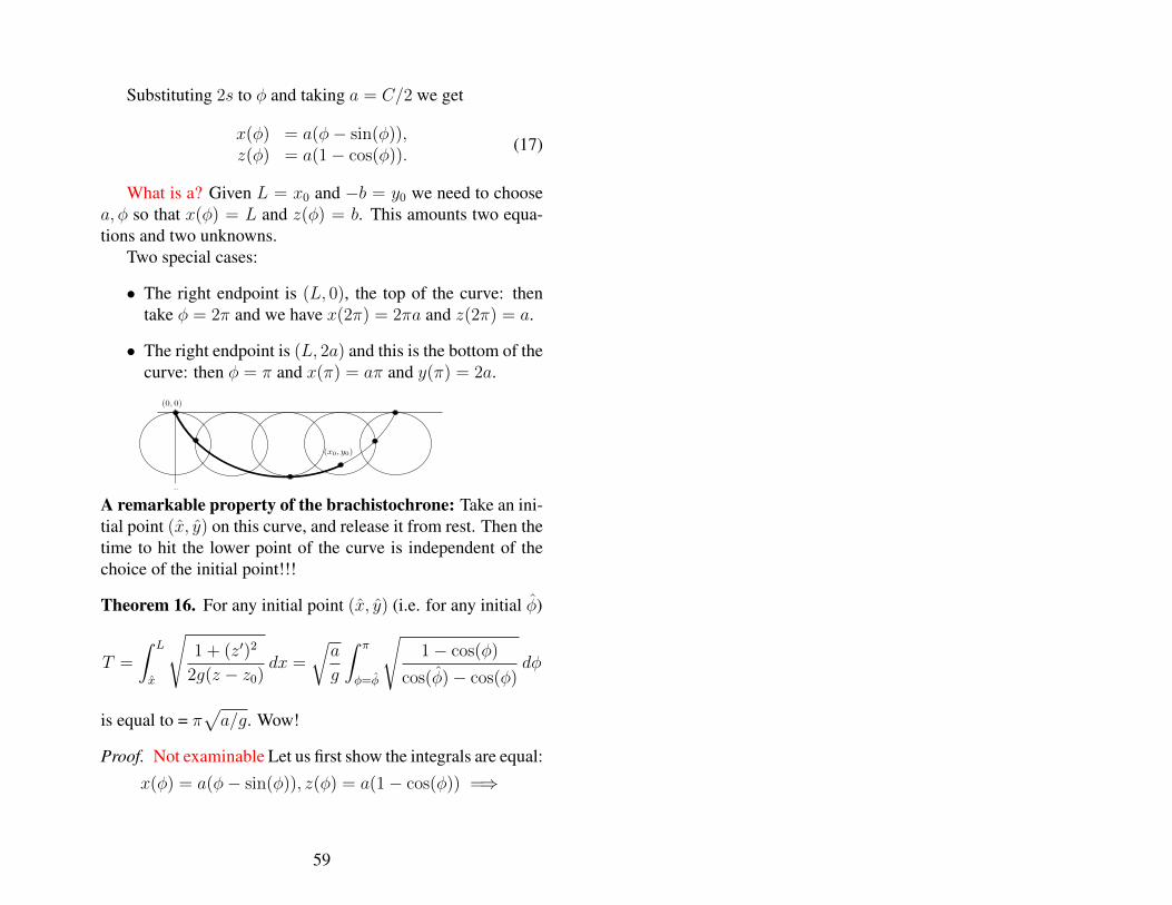
Substituting 2s to φ and taking a = C/2 we get

x(φ) = a(φ− sin(φ)),z(φ) = a(1− cos(φ)).

(17)

What is a? Given L = x0 and −b = y0 we need to choosea, φ so that x(φ) = L and z(φ) = b. This amounts two equa-tions and two unknowns.

Two special cases:

• The right endpoint is (L, 0), the top of the curve: thentake φ = 2π and we have x(2π) = 2πa and z(2π) = a.

• The right endpoint is (L, 2a) and this is the bottom of thecurve: then φ = π and x(π) = aπ and y(π) = 2a.

2.2. Calculus of variations: some classical problems 33

PSfrag replacements

!y

!x

!s

Figure 2.4: Element of arc length.

Hence the time of descent is given by

T =

!

curve

ds!2gy

=1!2g

! y0

0

"##$1 +%

dxdy

&2

ydy.

Our problem is to find the path {x(y), y " [0, y0]}, satisfying x(0) = 0 and x(y0) = x0, whichminimizes T , that is, to determine the minimizer for the function I : S # R, where

I(x) =1!2g

! y0

0

'1 + (x!(y))2

y

( 12

dy, x " S,

and S = {x " C1[0, y0] | x(0) = 0 and x(y0) = x0}. Here2 F (", #, $) =)

1+!2

" is independent of

", and so the Euler-Lagrange equation becomes

d

dy

*x!(y)+

1 + (x!(y))21!y

,= 0.

Integrating with respect to y, we obtain

x!(y)+1 + (x!(y))2

1!y

= C,

where C is a constant. It can be shown that the general solution of this di!erential equation isgiven by

x(") =1

2C2(" $ sin ") + C, y(") =

1

2C2(1 $ cos"),

where C is another constant. The constants are chosen so that the curve passes through the points(0, 0) and (x0, y0).

PSfrag replacements

(0, 0)

(x0, y0)

x

y

Figure 2.5: The cycloid through (0, 0) and (x0, y0).

This curve is known as a cycloid, and in fact it is the curve described by a point P in a circlethat rolls without slipping on the x axis, in such a way that P passes through (x0, y0); see Figure2.5.

2Strictly speaking, the F here does not satisfy the demands made in Theorem 2.1.1. Notwithstanding this fact,with some additional argument, the solution given here can be fully justified.

A remarkable property of the brachistochrone: Take an ini-tial point (x, y) on this curve, and release it from rest. Then thetime to hit the lower point of the curve is independent of thechoice of the initial point!!!

Theorem 16. For any initial point (x, y) (i.e. for any initial φ)

T =

∫ L

x

√1 + (z′)2

2g(z − z0)dx =

√a

g

∫ π

φ=φ

√1− cos(φ)

cos(φ)− cos(φ)dφ

is equal to = π√a/g. Wow!

Proof. Not examinable Let us first show the integrals are equal:

x(φ) = a(φ− sin(φ)), z(φ) = a(1− cos(φ)) =⇒

59

z′ =dz

dx=

dz

dφdx

dφ

=a sin(φ)

a(1− cos(φ))=⇒

√1 + (z′)2 =

√(1− cos(φ))2 + sin2(φ)

(1− cos(φ))2=

√2(1− cos(φ))

(1− cos(φ))2.

x(φ) = a(φ− sin(φ)), z(φ) = a(1− cos(φ)) =⇒

z′ =dz

dx=

dz

dtdx

dt

=a sin(φ)

a(1− cos(φ))=⇒

√1 + (z′)2 =

√(1− cos(φ))2 + sin2(φ)

(1− cos(φ))2=

√2(1− cos(φ))

(1− cos(φ))2.

Since dx = a(1− cos(φ)) dφ this gives√

1 + (z′)2

2g(z − z0)dx =

√a√g

√1− cos(φ)

cos(φ)− cos(φ)dφ.

Showing the two integrals the same.Claim: the following integral does not depend on φ:

∫ π

φ=φ

√1− cos(φ)

cos(φ)− cos(φ)dφ

Substitute sin(φ/2) =√

1− cosφ/√

2 and cosφ = 2 cos2(φ/2)−1 gives:√

1− cos(φ)

cos(φ)− cos(φ)=√

2sin(φ/2)√

2[cos2(φ/2)− cos2(φ/2)]

60

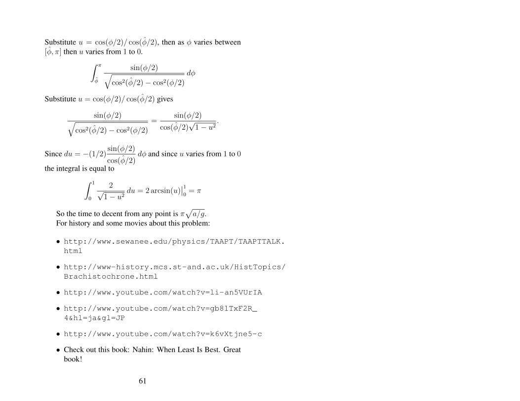
Substitute u = cos(φ/2)/ cos(φ/2), then as φ varies between[φ, π] then u varies from 1 to 0.

∫ π

φ

sin(φ/2)√cos2(φ/2)− cos2(φ/2)

dφ

Substitute u = cos(φ/2)/ cos(φ/2) gives

sin(φ/2)√cos2(φ/2)− cos2(φ/2)

=sin(φ/2)

cos(φ/2)√

1− u2.

Since du = −(1/2)sin(φ/2)

cos(φ/2)dφ and since u varies from 1 to 0

the integral is equal to∫ 1

0

2√1− u2

du = 2 arcsin(u)∣∣10

= π

So the time to decent from any point is π√a/g.

For history and some movies about this problem:

• http://www.sewanee.edu/physics/TAAPT/TAAPTTALK.html

• http://www-history.mcs.st-and.ac.uk/HistTopics/Brachistochrone.html

• http://www.youtube.com/watch?v=li-an5VUrIA

• http://www.youtube.com/watch?v=gb81TxF2R_4&hl=ja&gl=JP

• http://www.youtube.com/watch?v=k6vXtjne5-c

• Check out this book: Nahin: When Least Is Best. Greatbook!

61

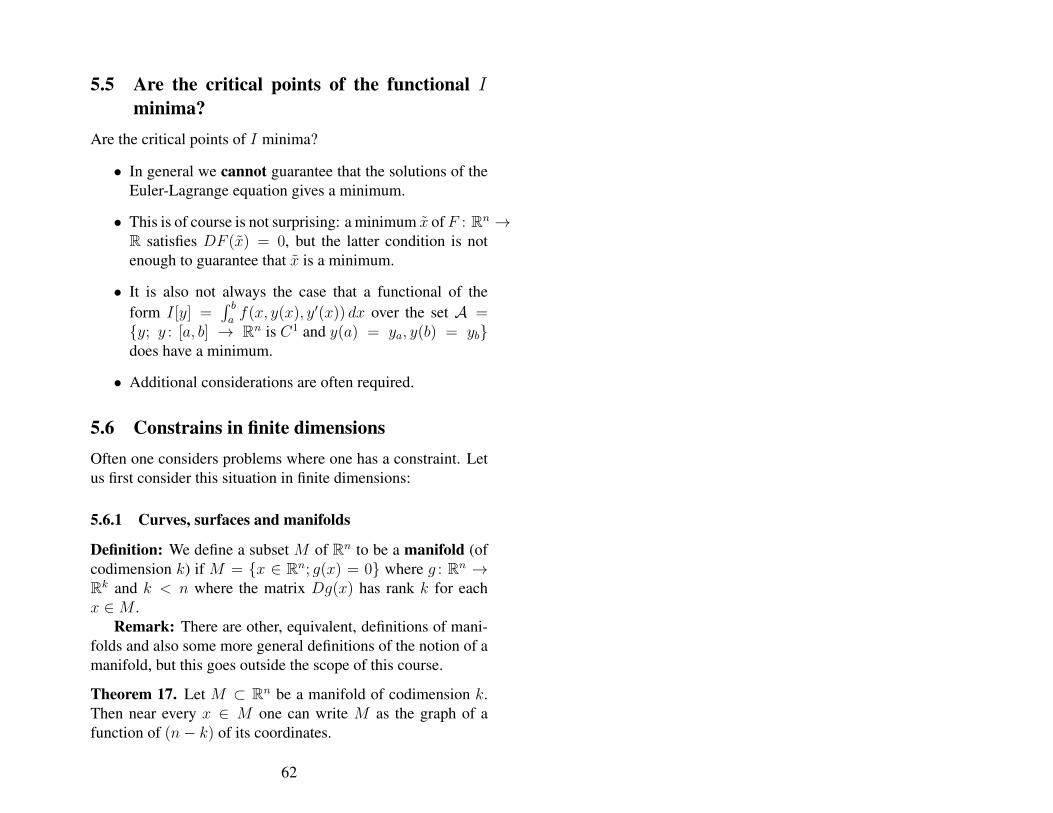
5.5 Are the critical points of the functional Iminima?

Are the critical points of I minima?

• In general we cannot guarantee that the solutions of theEuler-Lagrange equation gives a minimum.

• This is of course is not surprising: a minimum x ofF : Rn →R satisfies DF (x) = 0, but the latter condition is notenough to guarantee that x is a minimum.

• It is also not always the case that a functional of theform I[y] =

∫ baf(x, y(x), y′(x)) dx over the set A =

{y; y : [a, b] → Rn is C1 and y(a) = ya, y(b) = yb}does have a minimum.

• Additional considerations are often required.

5.6 Constrains in finite dimensionsOften one considers problems where one has a constraint. Letus first consider this situation in finite dimensions:

5.6.1 Curves, surfaces and manifolds

Definition: We define a subset M of Rn to be a manifold (ofcodimension k) if M = {x ∈ Rn; g(x) = 0} where g : Rn →Rk and k < n where the matrix Dg(x) has rank k for eachx ∈M .

Remark: There are other, equivalent, definitions of mani-folds and also some more general definitions of the notion of amanifold, but this goes outside the scope of this course.

Theorem 17. Let M ⊂ Rn be a manifold of codimension k.Then near every x ∈ M one can write M as the graph of afunction of (n− k) of its coordinates.

62

Examples. M = {(x, y) ∈ R2;x2 + y2 = 1} can bedescribed locally in the form x 7→ (x, y(x)) or in the formy 7→ (x(y), y).

Proof. Consider x0 ∈ M and for simplicity assume that thelast k columns of the k × n matrix Dg(x) are linearly inde-pendent. Then the k × k matrix made up of the last k columnsof the k × n matrix Dg(x) is invertible. This puts us in theposition of the Implicit Function Theorem. Indeed, write x =(u, v) ∈ Rn−k ⊕ Rk. The Implicit Function Theorem impliesthat there exists a function G : Rn−k → Rk so that

g(u, v) = 0 ⇐⇒ v = G(u).

SoM is locally a graph of a functionG: the set is locally of theformM = {(u,G(u));u ∈ Rn−k}. (If some other combinationof columns of Dg(x) are linearly independent then we arguesimilarly.)

Examples:

• Assume that g : R3 → R and consider M = {x ∈Rn; g(x) = 0}. Moreover assume that Dg(x) 6= 0 foreach x ∈ M . Then M is a surface. Any (orientable)surface can be written in this form.

• The set x2 +2y2 = 1, x2 +y4 +z6 = 1 is a codimension-two manifold (i.e. a curve) in R3.

Definition: The tangent plane at x ∈ M is defined as thecollection of vectors v ∈ Rn (based at x) so that Dgx(v) = 0.

To motivate this definition consider a C1 curve γ : [0, 1]→M ⊂ Rn with γ(0) = x. Since γ(t) ∈ M , it follows thatg ◦ γ(t) = 0 for all t and therefore

∂g

∂x1

(x)γ′1(0) + · · ·+ ∂g

∂xn(x)γ′n(0) = 0.

63

This if we write v = γ′(0) then Dg(x)v = 0. Hence 0 =Dg(x)v = ∇g(x) · v where · is the usual dot product in Rn.So the vector ∇g(x) is orthogonal to v := γ′(0) for each suchcurve γ.

5.6.2 Minima of functions on constraints (manifolds)

Suppose x is minimum of F : M → R where M = {x ∈Rn; g(x) = 0} and g : Rn → R. What does this imply? Writex = (x1, . . . , xn−1, xn).

Theorem 18. (Lagrange multiplier) If Dg(x) 6= 0 and x isminimum ofF : M → R, then ∃λ ∈ R withDF (x) = λDg(x).

Proof. Since Dg(x) 6= 0, we get that∂g

∂xi(x) 6= 0 for some

i = 1, . . . , n. In order to be definite assume∂g

∂xn(x) 6= 0

and write w = (x1, . . . , xn−1). By the Implicit Function The-orem, locally near w there exits h so that g(x) = 0 ⇐⇒xn = h(x1, . . . , xn−1). So w is minimum of (x1, . . . , xn−1) 7→F ◦ (x1, x2, . . . , xn−1, h(x1, . . . , xn−1)). This means for alli = 1, . . . , n− 1:

∂F

∂xi(x) +

∂F

∂xn(x)

∂h

∂xi(w) = 0.

Since g(x1, . . . , xn−1, h(x1, . . . , xn−1)) = 0 we also get

∂g

∂xi(x) +

∂g

∂xn(x)

∂h

∂xi(w) = 0 ∀i = 1, . . . , n− 1.

Substituting these into the previous equation and writing

λ =

∂F

∂xn(x)

∂g

∂xn(x)

64

gives

∂F

∂xi(x)− λ ∂g

∂xi(x) = 0 ∀i = 1, . . . , n− 1.

(For i = n the last equation also holds, by definition.)

5.7 Constrained Euler-Lagrange Equations

Let I[y] =∫ baf(x, y(x), y′(x)) dx and J [y] =

∫ bag(x, y(x), y′(x)) dx

be functionals on

A = {y; y : [a, b]→ Rn is C1 and y(a) = ya, y(b) = yb}.

as before. Define

M = {y; y ∈ A with J [y] = 0}.

Theorem 19. If M 3 y 7→ I[y] has a minimum at y then thereexists λ ∈ R so that the E-L condition hold for F = f − λg.That is,

d

dxFy′ [y] = Fy[y].

The idea of the proof combines the Lagrange multiplier ap-proach with the proof of the previous Euler Lagrange theorem.

Example 30. Maximize the area bounded between the graph ofy and the line segment [−1, 1]×{0}, conditional on the lengthof the arc being L. (This is a special case of Dido’s problem.)

Let A be the set of C1 functions y : [−1, 1] → R withy(−1) = y(1) = 0. Fix L > 0 and let

I[y] =

∫ 1

1

y(x) dx and J [y] =

∫ 1

−1

√1 + (y′)2 dx− L = 0.

65

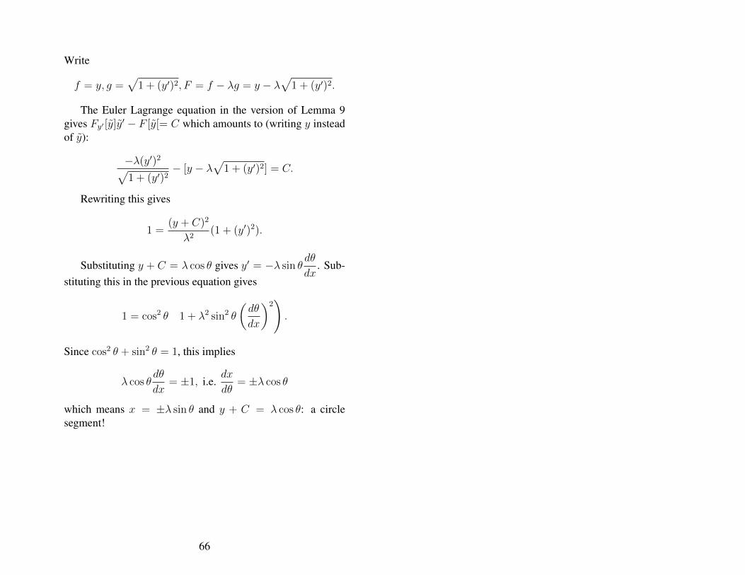
Write

f = y, g =√

1 + (y′)2, F = f − λg = y − λ√

1 + (y′)2.

The Euler Lagrange equation in the version of Lemma 9gives Fy′ [y]y′ − F [y[= C which amounts to (writing y insteadof y):

−λ(y′)2

√1 + (y′)2

− [y − λ√

1 + (y′)2] = C.

Rewriting this gives

1 =(y + C)2

λ2(1 + (y′)2).

Substituting y + C = λ cos θ gives y′ = −λ sin θdθ

dx. Sub-

stituting this in the previous equation gives

1 = cos2 θ

(1 + λ2 sin2 θ

(dθ

dx

)2).

Since cos2 θ + sin2 θ = 1, this implies

λ cos θdθ

dx= ±1, i.e.

dx

dθ= ±λ cos θ

which means x = ±λ sin θ and y + C = λ cos θ: a circlesegment!

66

6 Nonlinear TheoryIn the remainder of this course we will study initial value prob-lems associated to autonomous differential equations

x′ = f(x), x(0) = x0 (18)

where f : Rn → Rn is C∞. We saw:

• There exists δ(x0) > 0 so that this has a unique solutionx : (−δ, δ)→ Rn;

• There exists a unique maximal domain of existence I(x0) =(α(x0), β(x0)) and a unique maximal solution x : I(x0)→Rn.

• If β(x0) <∞ then |x(t)| → ∞ when t ↑ β(x0).

• If α(x0) > −∞ then |x(t)| → ∞ when t ↓ α(x0).

• The solution is often denoted by φt(x0).

• One has the flow property: φt+s(x0) = φtφs(x0), φ0(x0) =x0.

• Solutions do not intersect. One way of making this pre-cise goes as follows: t > s and φt(x) = φs(y) impliesφt−s(x) = y. (So φs(φt−s(x)) = φt(x) = φs(y) impliesφt−s(x) = y.)

6.1 The orbits of a flowRather than studying each initial value problem separately, itmakes sense to study the flow φt associated to x′ = f(x), x(0) =x0. The curves t 7→ φt(x) are called the orbits. For examplewe will show that the flow of

x = Ax−Bxyy = Cy +Dxy

is equal to

67

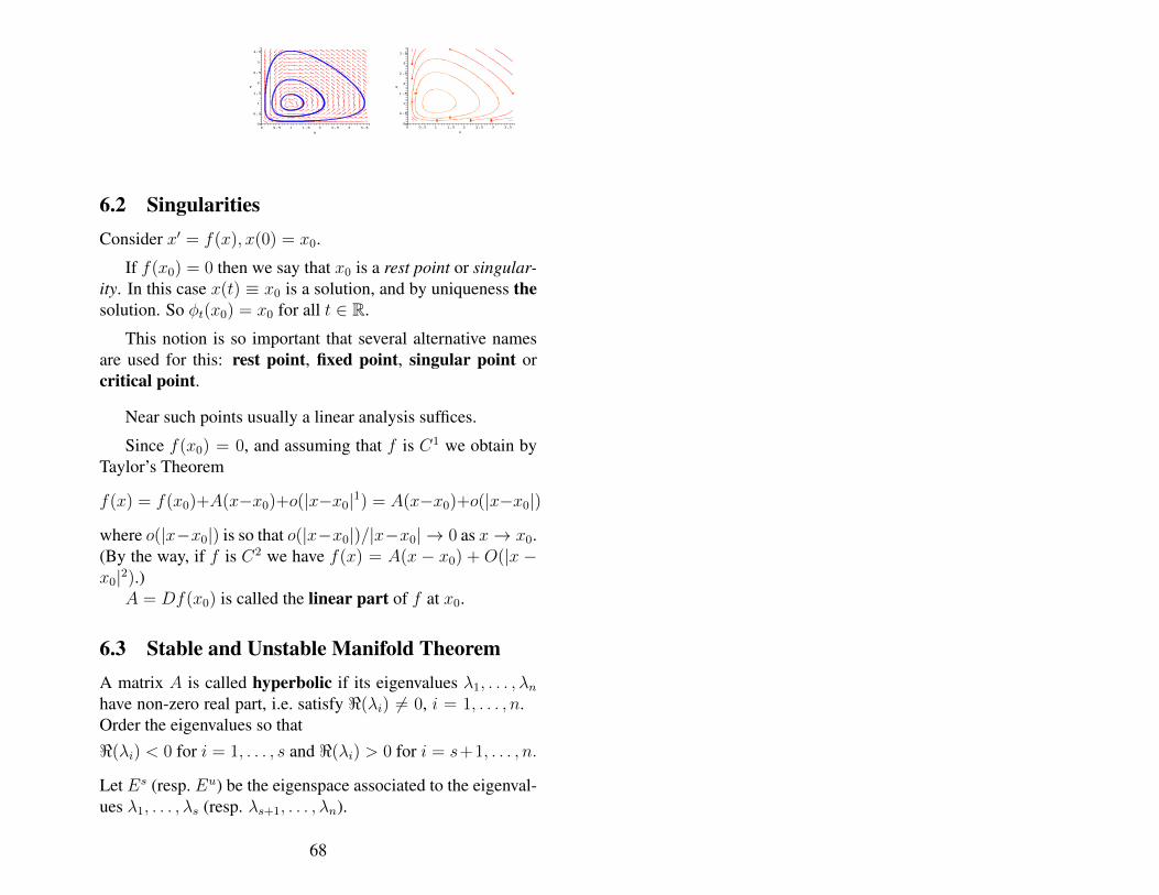
MathCapstone.pdf http://www.cs.utexas.edu/~schrum2/MathCapstone.pdf

5 of 23 23/02/2013 10:47

y

3.5

3

2.5

2

1.5

1

0.5

0

x

3.532.521.510.50

y

3

1

3.5

2.5

0.5

21.5 2.5

1.5

2

3 3.50.50

x

10

MathCapstone.pdf http://www.cs.utexas.edu/~schrum2/MathCapstone.pdf

6 of 23 23/02/2013 10:47

6.2 SingularitiesConsider x′ = f(x), x(0) = x0.

If f(x0) = 0 then we say that x0 is a rest point or singular-ity. In this case x(t) ≡ x0 is a solution, and by uniqueness thesolution. So φt(x0) = x0 for all t ∈ R.

This notion is so important that several alternative namesare used for this: rest point, fixed point, singular point orcritical point.

Near such points usually a linear analysis suffices.

Since f(x0) = 0, and assuming that f is C1 we obtain byTaylor’s Theorem

f(x) = f(x0)+A(x−x0)+o(|x−x0|1) = A(x−x0)+o(|x−x0|)

where o(|x−x0|) is so that o(|x−x0|)/|x−x0| → 0 as x→ x0.(By the way, if f is C2 we have f(x) = A(x − x0) + O(|x −x0|2).)

A = Df(x0) is called the linear part of f at x0.

6.3 Stable and Unstable Manifold TheoremA matrix A is called hyperbolic if its eigenvalues λ1, . . . , λnhave non-zero real part, i.e. satisfy <(λi) 6= 0, i = 1, . . . , n.Order the eigenvalues so that<(λi) < 0 for i = 1, . . . , s and <(λi) > 0 for i = s+1, . . . , n.

Let Es (resp. Eu) be the eigenspace associated to the eigenval-ues λ1, . . . , λs (resp. λs+1, . . . , λn).

68

A singular point x0 of f is called hyperbolic if the matrixDf(x0) is hyperbolic.

Theorem 20. Stable and Unstable Manifold Theorem Letx0 be a singularity of f and assume x0 is hyperbolic. Thenthere exist a manifold W s(x0) of dimension s and a manifoldW u(x0) of dimension n− s both containing x0 so that

x ∈ W s(x0) =⇒ φt(x)→ x0 as t→∞,

x ∈ W u(x0) =⇒ φt(x)→ x0 as t→ −∞.W s(x0),W u(x0) are tangent to x0 + Es resp. x0 + Eu at x0.

Remarks:

• Remember the notion of a manifold was defined in theprevious chapter. Most of the time we will consider thecase dimension one (then it is a curve) or of dimensiontwo (then it is a surface.

• If s = n then the singularity is called a sink.

• If 1 ≤ s < n then it is called a saddle.

• s = 0 then it called a source.

• W s(x0) is called the stable manifold.

• W u(x0) is called the unstable manifold.

Example 31. Take x′ = x + y2, y′ = −y + x2. By Theo-rem 20 there is supposed to an invariant manifold W u(0) (acurve) which is tangent to the x-axis. How to find the powerseries expansion ofW u(0)? Of course this is the same exampleas described in Chapter 3, but let us redo it here:

y′(x) = (dy

dt)/(

dx

dt) =−y + x2

x+ y2. (19)

69

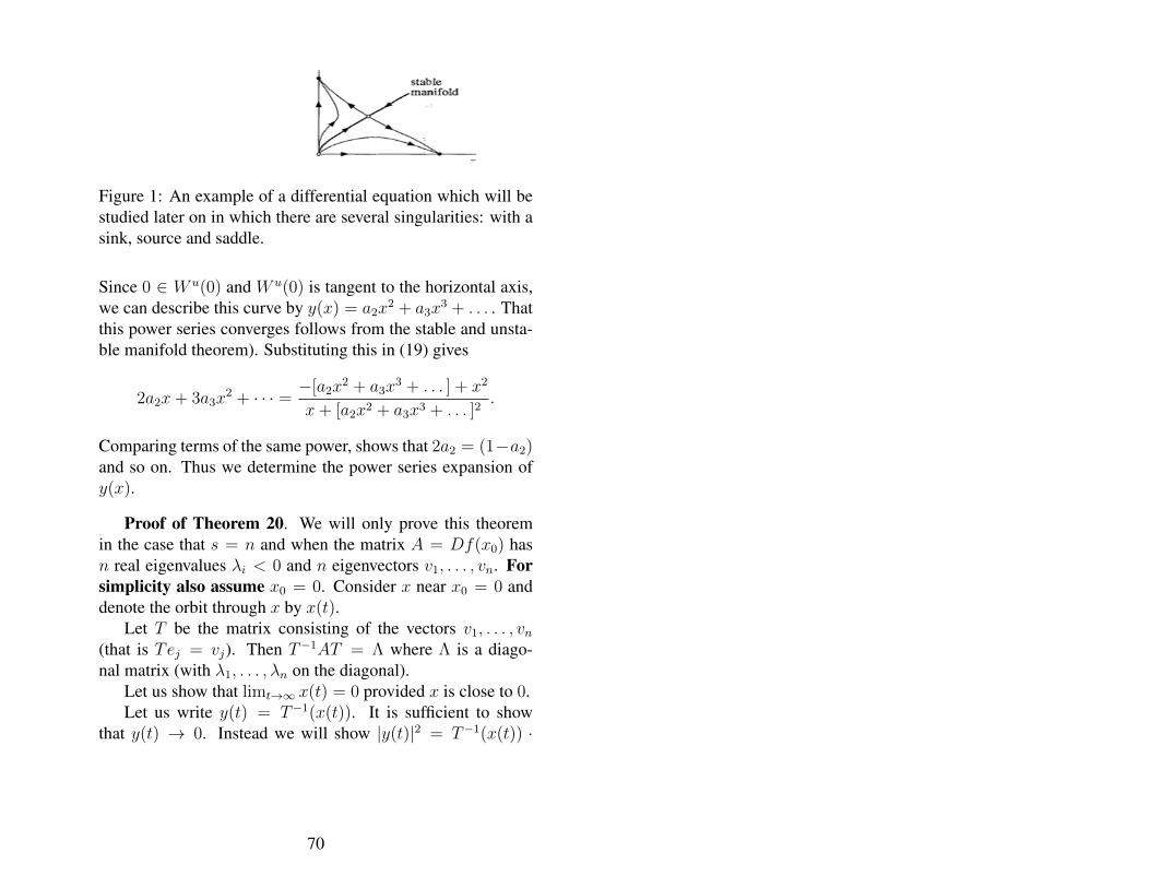
10.5923.j.fph.20130301.01_013.gif (PNG Image, 195 × 182 p... http://article.sapub.org/image/10.5923.j.fph.20130301.01_013.gif

1 of 1 23/02/2013 14:05

Figure 1: An example of a differential equation which will bestudied later on in which there are several singularities: with asink, source and saddle.

Since 0 ∈ W u(0) and W u(0) is tangent to the horizontal axis,we can describe this curve by y(x) = a2x

2 + a3x3 + . . . . That

this power series converges follows from the stable and unsta-ble manifold theorem). Substituting this in (19) gives

2a2x+ 3a3x2 + · · · = −[a2x

2 + a3x3 + . . . ] + x2

x+ [a2x2 + a3x3 + . . . ]2.

Comparing terms of the same power, shows that 2a2 = (1−a2)and so on. Thus we determine the power series expansion ofy(x).

Proof of Theorem 20. We will only prove this theoremin the case that s = n and when the matrix A = Df(x0) hasn real eigenvalues λi < 0 and n eigenvectors v1, . . . , vn. Forsimplicity also assume x0 = 0. Consider x near x0 = 0 anddenote the orbit through x by x(t).

Let T be the matrix consisting of the vectors v1, . . . , vn(that is Tej = vj). Then T−1AT = Λ where Λ is a diago-nal matrix (with λ1, . . . , λn on the diagonal).

Let us show that limt→∞ x(t) = 0 provided x is close to 0.Let us write y(t) = T−1(x(t)). It is sufficient to show

that y(t) → 0. Instead we will show |y(t)|2 = T−1(x(t)) ·

70

T−1(x(t))→ 0 as t→∞.

d|y(t)|2dt

=d

dt(T−1x(t) · T−1(x(t)) = 2T−1x · T−1x

= 2T−1x · T−1f(x)

= 2T−1x · T−1Ax+ 2T−1x · T−1[f(x)− Ax].

Let us first estimate the first term in this sum under the as-sumption that all eigenvalues of A are real. Then

T−1x · T−1Ax = y · Λy ≤ −ρ|y|2 (20)

where ρ = mini=1,...,n |λi|. Here we use that Λ is diagonal withall eigenvalues real (and therefore the eigenvectors are real andso T and y are also real).

The second term can be estimated as follows: Since f(x)−Ax = o(|x|) for any ε > 0 there exists δ > 0 so that |f(x) −Ax| ≤ ε|x| provided |x| ≤ δ. Hence using the Cauchy inequal-ity and the matrix norm we get

T−1x·T−1[f(x)−Ax] ≤ ε|y|·|T−1[f(x)−Ax]| ≤ |y|·||T−1||·ε|x|.provided |x| ≤ δ. Of course we have that |x| = |TT−1x| =|Ty| ≤ ||T || · |y|. Using this in the previous inequality gives

2T−1x · T−1[f(x)− Ax] ≤ 2ε||T || · ||T−1|| · |y|2. (21)

Using (20) and (21) in the estimate ford|y(t)|2dt

gives

d|y(t)|2dt

≤ −2ρ|y(t)|2 + 2ε||T || · ||T−1|| · |y(t)|2 ≤ −ρ′|y(t)|2

where ρ′ = (2ρ − 2ε||T || · ||T−1||). Provided we take ε > 0sufficiently small we get that ρ′ > 0. That is if we write z(t) =|y(t)|2 then we get z′ ≤ −ρ′z which means

|y(t)|2 = z(t) ≤ z(0)e−tρ′ ≤ |y(0)|2e−tρ′

71

and therefore that |y(t)| → 0 as t → ∞ (with a rate which isrelated to ρ′/2 (which is close to ρ if we choose ε > 0 small).

IfA is diagonalisable but the eigenvalues are no longer real,then the estimate in the inequality in (20) needs to be alteredslightly. Let us explain the required change by considering an

example. Take A =

(−a b−b −a

). Note A has eigenvalues

−a ± bi and that A is already in the real Jordan normal form.Moreover,

y · Ay =

(y1

y2

)·(−ay1 + by2

−by1 − ay2

)

= −a([y1(t)]2 + [y2(t)]2

)= −a|y|2.

so the argument goes through. Using the real Jordan normalform theorem, the same method applies as long asA has a basisof n eigenvectors. This concludes the proof of Theorem 20 inthis setting. We will skip the prove in the general setting, butthe next example shows what happens if there is no basis ofeigenvectors.

In fact, when we prove that x(t) by showing that |y(t)|2tends to zero, we use the function U(x) := |T−1(x)|2. Laterwe will call this a Lyapounov function.

Example 32. Let us consider a situation when the matrix does

not have a basis of eigenvectors. LetA =

(−1 Z0 −1

)where

Z ∈ R. This has eigenvalues −1 (with double multiplicity).Take U(x, y) = ax2 + bxy + cy2. Then

U = 2axx+ bxy + bxy + 2cyy= 2ax(−x+ Zy) + b(−x+ Zy)y + bx(−y) + 2cy(−y)= −2ax2 + (2Za− b− b)xy + (Zb− 2c)y2.

72

Case 1: If Z ≈ 0, then we can take a = 1, b = 0, c = 1because then U = −2x2 + (2Z)xy − 2y2 ≤ 0 (since Z ≈ 0).

Case 2: If Z is large and a = 1, b = 0, c = 1 then wedefinitely don’t get U ≤ 0. However, in this case we can setb = 0, and write

U = −2ax2 + (2Za)xy − 2cy2

= −2a[x− (Z/2)y]2 + (aZ2/2− 2c)y2

= −2[x− (Z/2)y]2 − y2 < 0.

where in the last line we substitutes a = 1 and c = 1/2+Z2/4.Thus U = c corresponds to a ‘flat’ ellipse when Z is large.

General case: This all seems rather ad hoc, but the Jor-dan normal form suggests a general method. Indeed A has

an eigenvector v1 =

(10

)(i.e. (A + I)v1 = 0) and we

can choose a 2nd vector v2 so that (A + I)v2 = εv1 where

ε > 0 is small. So v2 =

(0ε/Z

). Taking T = (v1v2) gives

T−1AT =

(−1 ε0 −1

). In this new coordinates we are in

the same position as if Z ≈ 0. So we can argue as in the firstcase.

6.4 Hartman-GrobmanTheorem 21. Hartman-Grobman Let x0 be a singularityand that A = Df(x0) is a hyperbolic matrix. Then there existsa continuous bijection (a homeomorphism) h : Rn → Rn sothat h(x0) = 0 and so that near x0,

h sends orbits of x′ = f(x) to orbits of x′ = Ax.

Remark: In other words, there exists an open set U 3 x0 sothat

h ◦ φt(x) = φAt ◦ h(x)

73

for each x, t so that

∪0≤s≤tφs(x) ⊂ U.

Here φAt is the flow associated to x′ = Ax and φt the flow forx′ = f(x).

Remark: A homeomorphism is a continuous bijection whoseinverse is also continuous. In Euclidean space (and ‘mani-folds’), this is the same as saying that it is continuous bijection.

6.5 Lyapounov functionsSometimes one applies a method which is similar to the proofgiven in Theorem 20, namely one uses a so-called Lyapounovfunction:

In actual fact, we will use the notion of Lyapounov func-tion more loosely, and for example sometimes give the samename to a function for which merely V ≤ 0.

Definition: Let W ⊂ Rn be an open set containing x0.V : W → R is a Lyapounov function for x0 if it is C1 and

• V (x0) = 0, V (x) > 0 for x ∈ W \ {x0};

• V ≤ 0 for x ∈ W .

Here V :=dV (x(t))

dt= DVx(t)

dx

dt= DVx(t)f(x(t)).

Remarks: V should be thought of as a way to measure thedistance to x0. That V ≤ 0 means that this ‘distance’ is non-increasing. In quite a few textbooks a Lyapounov function isone which merely satisfies the first property; let’s call suchfunctions weak-Lyapounov functions.

Warning: In some cases one calls a function Lyapounoveven if it does not satisfies all its properties.

Definitions:

• x0 is called asymptotically stable if, for each x near x0,one has φt(x)→ x0.

74

• x0 is called stable if for each ε > 0 there exists δ > 0 sothat if x ∈ Bδ(x0) implies φt(x) ∈ Bε(x0) for all t ≥ 0.(So you nearby points don’t go far.)

Lemma 10. Lyapounov functions

1. If V ≤ 0 then x0 is stable. Moreover, φt(x) exists for allt ≥ 0 provided d(x, x0) is small.

2. If V < 0 for x ∈ W \{x0} then ∀x is close to x0 one getsφt(x)→ x0 as t→∞, i.e. x0 is asymptotically stable.

Proof. (1) Take ε > 0 so that B2ε(x0) ⊂ W . Let

δ := infy∈∂Bε(x0)

V (y).

Since V > 0 except at x0 we get δ > 0. It follows that

V −1[0, δ) ∩ ∂Bε(x0) = ∅. (22)

Take x ∈ V −1[0, δ) ∩ Bε(x0) (this holds for all x near x0 bycontinuity of V and since V (0) = 0). Since φ0(x) = x andt → V (φt(x)) is non-increasing, φt(x) ∈ V −1[0, δ) for all t ≥0. Since t → φt(x) is continuous curve, φ0(x) = x ∈ Bε(x0)and (22), it follows that φt(x) ∈ Bε(x0) for all t ≥ 0. Inparticular φt(x) remains bounded, and so φt(x) exists ∀t.

(2) V < 0 implies that t → V (φt(x)) is strictly decreas-ing. Take x ∈ V −1[0, δ) ∩ Bε(x0) and suppose by contra-diction that V (φt(x)) does not tend to 0 as t → ∞. Then,since t 7→ V (φt(x)) is decreasing, there exists V0 > 0 so thatV (ρt(x)) ≥ V0 > 0. Hence ∃ρ > 0 with φt(x) /∈ Bρ(x0)∀t ≥ 0. Combining this with part (1) gives that

φt(x) ∈ Bε(x0) \Bρ(x0) for all t ≥ 0.

But V < 0, V is only zero at x0 and V attains its maximum ina compact set Bε(x0) \Bρ(x0) it follows that ∃κ > 0 so that

V ≤ −κ whenever x(t) ∈ Bε(x0) \Bρ(x0).

75

But since x(t) is in this compact set for all t ≥ 0,

V ≤ −κ,∀t ≥ 0.

Hence

V (φt(x))− V (x) ≤ −κt→ −∞ as t→∞,

contradicting V ≥ 0.

Example 33.x′ = 2y(z − 1)y′ = −x(z − 1)z′ = xy

Its linearisation is A :=

0 −2 01 0 00 0 0

. Note A has eigenval-

ues ±√

2i and 0. So A is not hyperbolic, and theorem 20 doesnot apply.

Take V (x, y, z) = ax2 + by2 + cz2. Then

V = 2(axx+byy+czz) = 4axy(z−1)−2bxy(z−1)+2cxyz.

We want V ≥ 0 and V ≤ 0. We can achieve this by settingc = 0, 2a = b. This makes V = 0. It follows that solutions stayon level sets of the function V = x2 +2y2. x0 = (0, 0, 0) is notasymptotically stable. Strictly speaking V is not a Lyapounovfunction because V (0, 0, z) = 0: more work needed to checkif x0 is stable.

Example 34. Consider the system x′ = −y−xy2, y′ = x−yx2.The only singularity of this system is at (0, 0). Indeed, if x′ =0, then either y = 0 or 1+xy = 0; if y = 0 then x(1−xy) = 0implies x = 0; if 1 + xy = 0 then 0 = x(1− xy) = 2x impliesx = 0 which contradicts 1 + xy = 0.

Let us show that (0, 0) is asymptotically stable. To do this,take the quadratic function V (x, y) = x2+y2. Then V = 2xx+

76

2yy = −2x2y2 ≤ 0, so (0, 0) is stable. Since V is decreasing(non-increasing), this implies that there exists V0 ≥ 0 so thatV (x(t), y(t)) ↓ V0. If V0 = 0 then the solution converges to(0, 0) as claimed. If V0 > 0 then the solution converges tothe circle {(x, y);x2 + y2 = V0}, and in particular remainsbounded. Note that the set V (x, y) = x2 + y2 = V0 does notcontain singular points and also is not a periodic orbit, sinceV < 0 except when x = 0 or y = 0. (By looking at the arrows,one concludes that the orbits are tangent to circles when x = 0or when y = 0 but otherwise spiral inwards.) It follows thatV0 = 0 and so we are done.

6.6 The pendulumConsider a pendulum moving along a circle of radius l, witha mass m and friction k. Let θ(t) be the angle from the ver-

tical at time t. The force tangential to the circle is −(kldθ

dt+

mg sin(θ)). So Newton’s law gives

mlθ′′ = −klθ′ −mg sin θ i.e. θ′′ = −(k/m)θ′ − (g/l) sin θ.

Taking ω = θ′ gives

θ′ = ω

ω′ =−gl

sin(θ)− k

mω.

Singularities are (nπ, 0) which corresponds to the pendulumbeing in vertical position (pointing up or down). Linearizingthis at (0, 0) gives

(0 1−g/l −k/m

)

which gives eigenvalues (−k/m±√

(k/m)2 − 4g/l)/2.

77

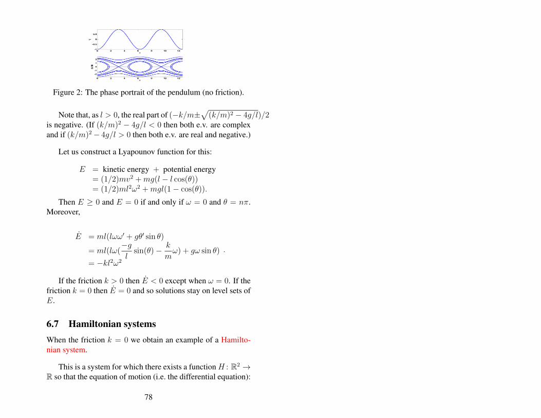
300px-Pendulumphase.png (PNG Image, 300 × 225 pixels) http://upload.wikimedia.org/wikipedia/commons/thumb/b/b7...

1 of 1 24/02/2013 15:20

Figure 2: The phase portrait of the pendulum (no friction).

Note that, as l > 0, the real part of (−k/m±√

(k/m)2 − 4g/l)/2is negative. (If (k/m)2 − 4g/l < 0 then both e.v. are complexand if (k/m)2− 4g/l > 0 then both e.v. are real and negative.)

Let us construct a Lyapounov function for this:

E = kinetic energy + potential energy= (1/2)mv2 +mg(l − l cos(θ))= (1/2)ml2ω2 +mgl(1− cos(θ)).

Then E ≥ 0 and E = 0 if and only if ω = 0 and θ = nπ.Moreover,

E = ml(lωω′ + gθ′ sin θ)

= ml(lω(−gl

sin(θ)− k

mω) + gω sin θ)

= −kl2ω2

.

If the friction k > 0 then E < 0 except when ω = 0. If thefriction k = 0 then E = 0 and so solutions stay on level sets ofE.

6.7 Hamiltonian systemsWhen the friction k = 0 we obtain an example of a Hamilto-nian system.

This is a system for which there exists a functionH : R2 →R so that the equation of motion (i.e. the differential equation):

78

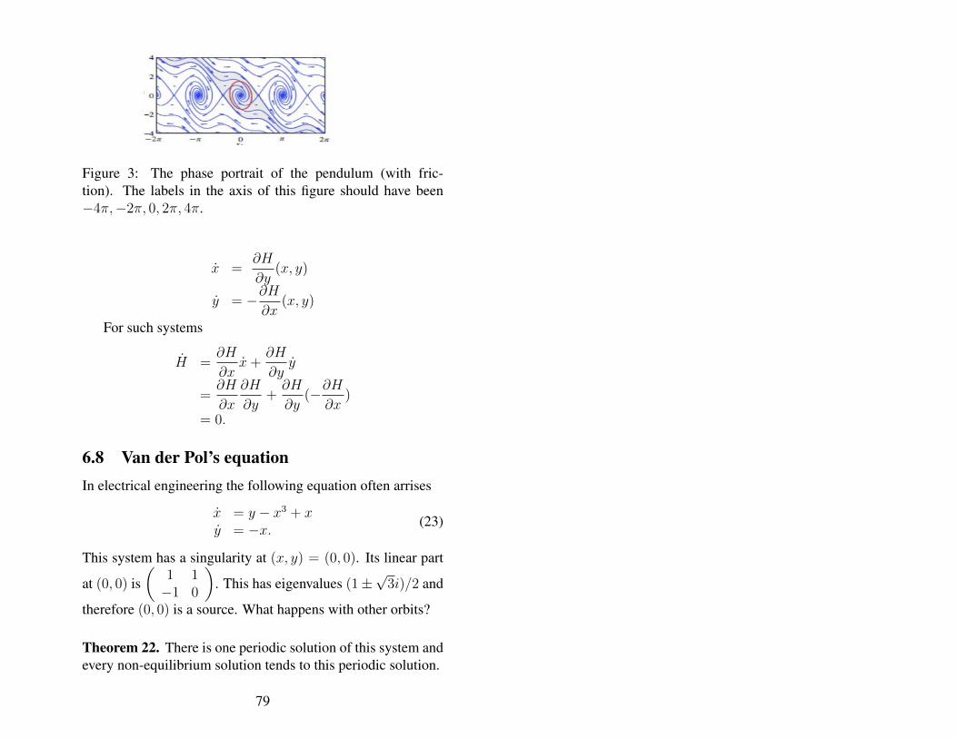
pendulum.preview.jpg (JPEG Image, 640 × 265 pixels) http://www.igorexchange.com/files/images/pendulum.preview.jpg

1 of 1 24/02/2013 16:19

Figure 3: The phase portrait of the pendulum (with fric-tion). The labels in the axis of this figure should have been−4π,−2π, 0, 2π, 4π.

x =∂H

∂y(x, y)

y = −∂H∂x

(x, y)

For such systems

H =∂H

∂xx+

∂H

∂yy

=∂H

∂x

∂H

∂y+∂H

∂y(−∂H

∂x)

= 0.

6.8 Van der Pol’s equationIn electrical engineering the following equation often arrises

x = y − x3 + xy = −x. (23)

This system has a singularity at (x, y) = (0, 0). Its linear part

at (0, 0) is(

1 1−1 0

). This has eigenvalues (1±

√3i)/2 and

therefore (0, 0) is a source. What happens with other orbits?

Theorem 22. There is one periodic solution of this system andevery non-equilibrium solution tends to this periodic solution.

79

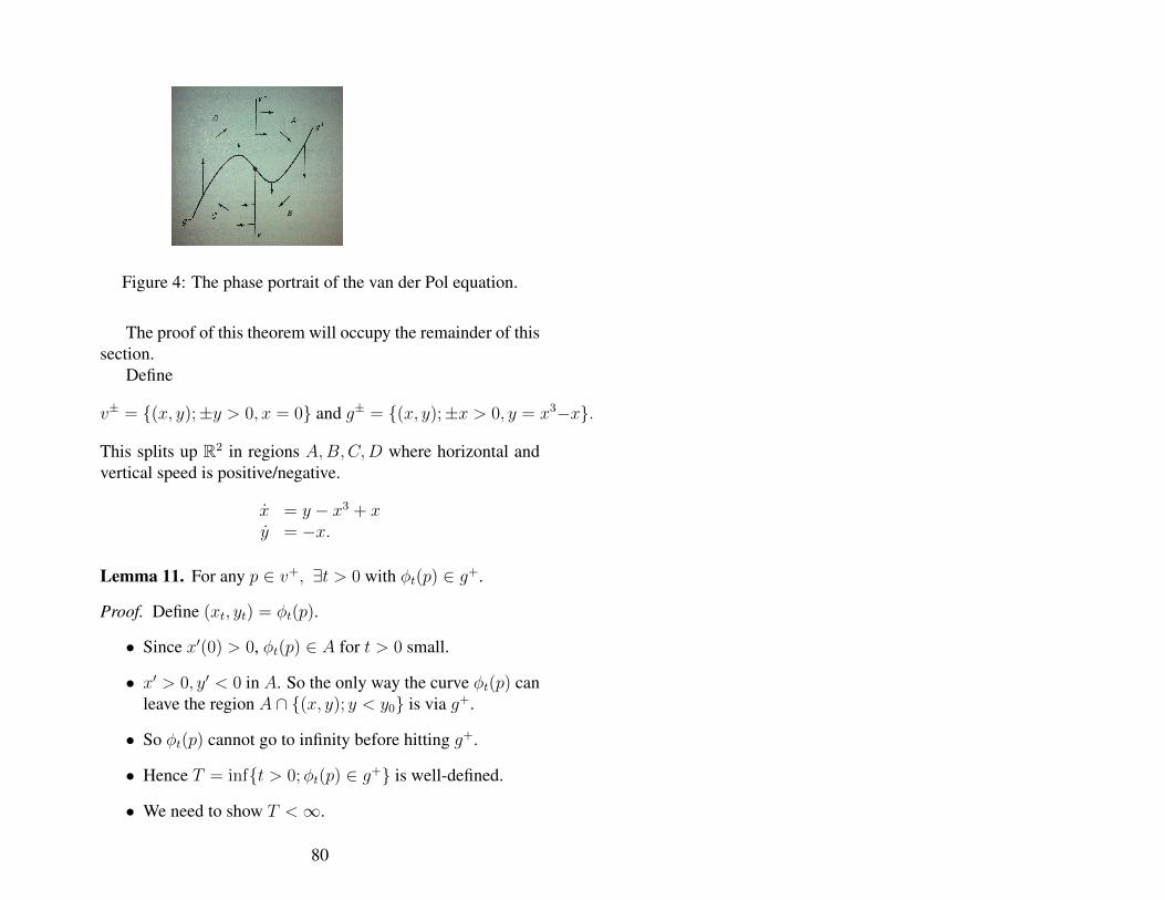
Figure 4: The phase portrait of the van der Pol equation.

The proof of this theorem will occupy the remainder of thissection.

Define

v± = {(x, y);±y > 0, x = 0} and g± = {(x, y);±x > 0, y = x3−x}.

This splits up R2 in regions A,B,C,D where horizontal andvertical speed is positive/negative.

x = y − x3 + xy = −x.

Lemma 11. For any p ∈ v+, ∃t > 0 with φt(p) ∈ g+.

Proof. Define (xt, yt) = φt(p).

• Since x′(0) > 0, φt(p) ∈ A for t > 0 small.

• x′ > 0, y′ < 0 in A. So the only way the curve φt(p) canleave the region A ∩ {(x, y); y < y0} is via g+.

• So φt(p) cannot go to infinity before hitting g+.

• Hence T = inf{t > 0;φt(p) ∈ g+} is well-defined.

• We need to show T <∞.

80

• Choose t0 ∈ (0, T ) and let a = xt0 . Then a > 0 andxt ≥ a for t ∈ [t0, T ].

• Hence y ≤ −a for t ∈ [t0, T ] and therefore y(t) −y(t0) ≤ −a(t− t0) for t ∈ [t0, T ].

• T = ∞ =⇒ limt→∞ y(t) → −∞ which gives a con-tradiction since (x(t), y(t)) ∈ A for t ∈ (0, T ).

Similarly

Lemma 12. For any p ∈ g+, ∃t > 0 with φt(p) ∈ v−.

For each y > 0 define F (y) = φt(0, y) where t > 0 is min-imal so that φt(0, y) ∈ v−. Similarly, define for y < 0 defineF (y) = φt(0, y) where t > 0 is minimal so that φt(0, y) ∈ v+.By symmetry F (−y) = −F (y).

Define the Poincaré first return map to v+ as

P : v+ → v+ by (0, y) 7→ (0, F 2(y)).

P (p) = φt(p) where t > 0 is minimal so that φt(p) ∈ v+.

Lemma 13. 1. P : v+ → v+ is increasing (here we orderv+ as (0, y1) < (0, y2) when y1 < y2);

2. P (p) > p when p ≈ 0;

3. P (p) < p when p is large;

4. P : v+ → v+ has a unique attracting fixed point.

81

Proof. The proof of (1): Uniqueness of solns =⇒ orbits don’tcross =⇒ P is increasing.

Instead of (2), (3) and (4) we shall prove the followingstatement:

p 7→ δ(p) := |F (p)|2 − |p|2 is strictly decreasing

δ(p) > 0 for p > 0 small and

δ(p)→ −∞ as p→∞

(24)

Note that this implies (2) and (3) and (4) (see lecture). SoTheorem 22 follows from (24).

Step 1: A useful expression for δ(p). Define

p∗ = (0, y∗) ∈ v+ so that ∃t with φt(p∗) = (1, 0)and φs(p∗) ∈ A for 0 < s < t.

Define U(x, y) = x2 + y2. Pick p ∈ v+ and let τ > 0 beminimal so that φτ (p) ∈ v−. (So φτ (p) = F (p).) Hence

δ(p) : = |F (p)|2 − |p|2 = U(φτ (p))− U(φ0(p))

=∫ τ

0U(φt(p)) dt.

Note

U = 2xx+ 2yy =

= 2x(y − x3 + x) + 2y(−x) = −2x(x3 − x) = 2x2(1− x2).

Hence

δ(p) = 2

∫ τ

0

[x(t)]2(1− [x(t)]2)dt = 2

∫

γ

x2(1− x2) dt.

Here γ is the curve [0, τ ] 3 t→ φt(p). If p < p∗ then δ(p) > 0because then (1− [x(t)]2) ≥ 0 for all t ∈ [0, τ ].

Step 2: δ(p) when p > p∗. We can decompose the curve γ inthree pieces as γ meets the line x = 1 twice

82

• the piece of γ with both endpoint on this line we call γ2;

• γ1 is the curve which connects p ∈ v+ to the line x = 1.

• γ3 is the curve which connects F (p) ∈ v− to the linex = 1.

Now consider

δi(p) := 2

∫

γi

x2(1− x2) ds for i = 1, 2, 3.

Step 3: δ1(p) is decreasing when p > p∗.

• γ1 is a curve which can be regarded as function of x.

• Hence we can write∫

γ1

x2(1−x2) dt =

∫

γ1

x2(1− x2)

dx/dtdx =

∫

γ1

x2(1− x2)

y − (x3 − x)dx.

• As p moves up, the curve γ1 (connecting p ∈ v+ to apoint on the line x = 1) moves up and so y − (x3 − x)(along this curve) increases.

• Hence p → δ1(p) = 2∫γ1x2(1 − x2) dt decreases as p

increases.

Step 4: δ2(p) is decreasing when p > p∗.

• Along γ2, x(t) is a function of y ∈ [y1, y2] (where (1, y1),y1 > 0 and (1, y2), y2 < 0) are the intersections points ofγ with the line x = 1.

• Since −x = dy/dt we get in the 2nd integral one has∫ y2y1

because that corresponds tothe way the curve γ1 is oriented.∫

γ1x2(1− x2) dt =

∫ y2y1−x(y)(1− [x(y)]2) dy

=∫ y1y2x(y)(1− [x(y)]2) dy

83

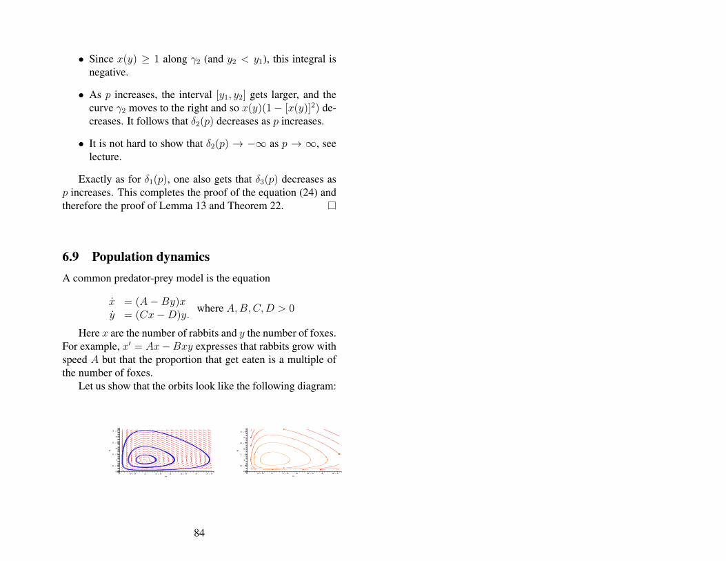
• Since x(y) ≥ 1 along γ2 (and y2 < y1), this integral isnegative.

• As p increases, the interval [y1, y2] gets larger, and thecurve γ2 moves to the right and so x(y)(1− [x(y)]2) de-creases. It follows that δ2(p) decreases as p increases.

• It is not hard to show that δ2(p) → −∞ as p → ∞, seelecture.

Exactly as for δ1(p), one also gets that δ3(p) decreases asp increases. This completes the proof of the equation (24) andtherefore the proof of Lemma 13 and Theorem 22.

6.9 Population dynamicsA common predator-prey model is the equation

x = (A−By)xy = (Cx−D)y.

where A,B,C,D > 0

Here x are the number of rabbits and y the number of foxes.For example, x′ = Ax−Bxy expresses that rabbits grow withspeed A but that the proportion that get eaten is a multiple ofthe number of foxes.

Let us show that the orbits look like the following diagram:

MathCapstone.pdf http://www.cs.utexas.edu/~schrum2/MathCapstone.pdf

5 of 23 23/02/2013 10:47

y

3.5

3

2.5

2

1.5

1

0.5

0

x

3.532.521.510.50

y

3

1

3.5

2.5

0.5

21.5 2.5

1.5

2

3 3.50.50

x

10

MathCapstone.pdf http://www.cs.utexas.edu/~schrum2/MathCapstone.pdf

6 of 23 23/02/2013 10:47

84

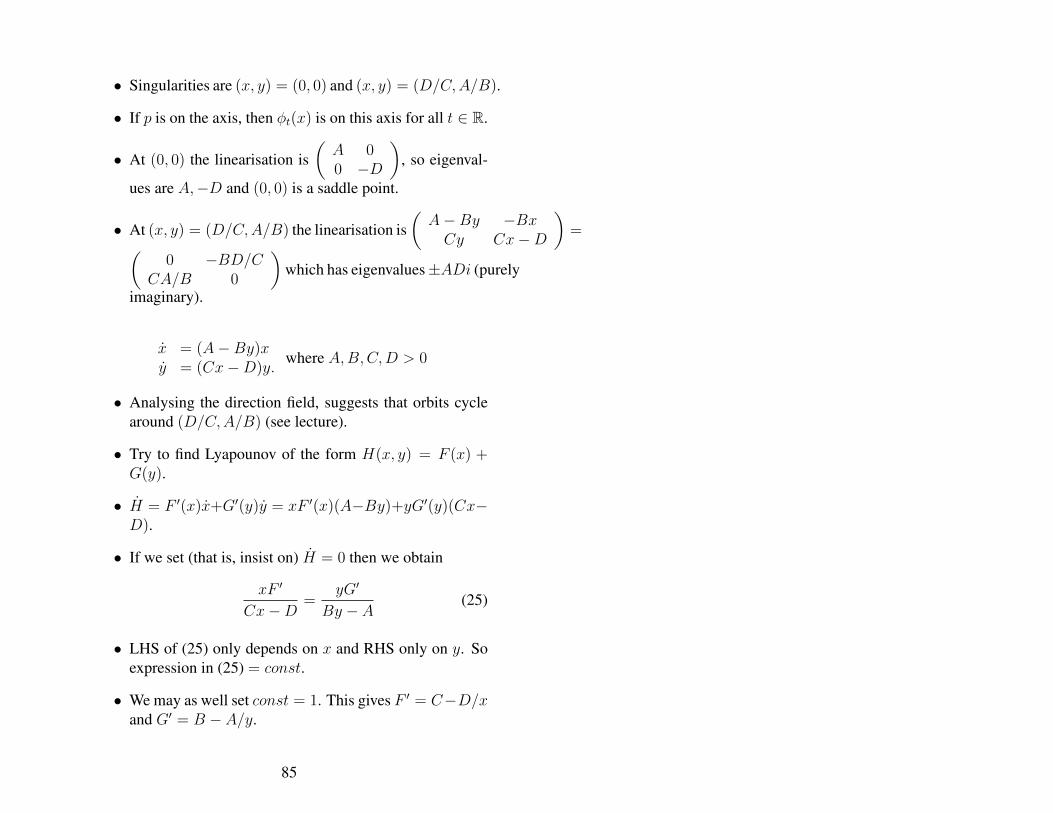
• Singularities are (x, y) = (0, 0) and (x, y) = (D/C,A/B).

• If p is on the axis, then φt(x) is on this axis for all t ∈ R.

• At (0, 0) the linearisation is(A 00 −D

), so eigenval-

ues are A,−D and (0, 0) is a saddle point.

• At (x, y) = (D/C,A/B) the linearisation is(A−By −BxCy Cx−D

)=

(0 −BD/C

CA/B 0

)which has eigenvalues±ADi (purely

imaginary).

x = (A−By)xy = (Cx−D)y.

where A,B,C,D > 0

• Analysing the direction field, suggests that orbits cyclearound (D/C,A/B) (see lecture).

• Try to find Lyapounov of the form H(x, y) = F (x) +G(y).

• H = F ′(x)x+G′(y)y = xF ′(x)(A−By)+yG′(y)(Cx−D).

• If we set (that is, insist on) H = 0 then we obtain

xF ′

Cx−D =yG′

By − A (25)

• LHS of (25) only depends on x and RHS only on y. Soexpression in (25) = const.

• We may as well set const = 1. This gives F ′ = C−D/xand G′ = B − A/y.

85

• So F (x) = Cx − D log x,G(y) = By − A log y andH(x, y) = Cx−D log x+By − A log y.

Summarising:

Theorem 23. Take (x, y) 6= (D/C,A/B) with x, y > 0 andconsider its orbits under

x = (A−By)xy = (Cx−D)y.

where A,B,C,D > 0.

Then t 7→ φt(x, y) is periodic (i.e. is a closed curve).

Proof. Take H0 = H(x, y) and let Σ = {(u, v);H(u, v) =H0}.

• The orbit φt(x, y) stays on the level set Σ of H .

• It moves with positive speed.

• So it returns in finite time.

• Orbits exist for all time, because it remains on Σ (andtherefore cannot go to infinity).

86

7 Dynamical SystemsSo far we saw:

• Most differential equations cannot be solved explicitly.

• Nevertheless in many instances one can still prove manyproperties of its solutions.

• The point of view taken in the field dynamical systems isto concentrate on

– attractors and limit sets: what happens eventually;

– statistical properties of orbits.

In this chapter we will discuss a result which describes theplanar case (i.e. the two-dimensional case).

Throughout the remainder of this notes, we will tacitly as-sume the solution φt(x) through x exists for all t ≥ 0.

7.1 Limit SetsLet φt be the flow of a dynamical system and take a point x.Then the ω-limit set of x, denoted by ω(x), is the set of limitpoints of the curve [0,∞) 3 t 7→ φt(x). More specifically,y ∈ ω(x) if and only if there exists a sequence tn →∞ so thatφtn(x)→ y.

So ω(x) describes where the point x eventually goes. It iseasy to prove that ω(x) is a closed set (see assignments). (But,possibly, ω(x) = ∅.)

We say that x lies on a periodic orbit if φT (x) = x for someT > 0. The smallest such T > 0 is called the period of x. Notethat then

87

• γ = ∪t∈[0,T )φt(x) is closed curve without self-intersections,and

• ω(x) = γ.

7.2 Local sectionsDefinition: We say that a manifold S 3 p of codimension-onein Rn is a local section at p for the autonomous differentialequation x′ = f(x) if:

1. S = {x ∈ Rn; g(x) = 0} contains p and Dg(p) 6= 0(hence is a manifold containing p);

2. f(p) 6= 0 and that Dg(p)f(p) 6= 0 (this means that f(p)does not lie in the tangent space of S at p).

Theorem 24 (Flow Box Theorem). Assume S is a local sec-tion at p and assume q is that φt0(q) = p for some t0 > 0.Then

• there exists a neighbourhood U of q;

• a smooth function τ : U → R so that τ(q) = t0 so thatfor each x ∈ U , φτ(x)(x) ∈ S.

If t0 > 0 is the minimal time so that φt0(q) ∈ S then we willalso have that τ(x) > 0 is minimal so that φτ(x)(x) ∈ S. τ(x)is then called the first arrival time and the map P (x) = φτ(x)(x)the Poincaré entry map to S.

Proof. DefineG(x, t) = g(φt(x)). ThenG(q, t0) = g(φt0(q)) =g(p) = 0. Moreover,

∂G

∂t(q, t0) = Dg(φt0(q))

∂φt∂t

(q)∣∣t=t0

= Dg(p)f(φt0(q))

= Dg(p)f(p) 6= 0 (because S is a section at p).

88

Hence by the implicit function theorem there exists x 7→ τ(x)so that G(x, τ(x)) = 0 for x near q. Hence φτ(x) ∈ S for xnear q.

Remarks:

1. If S is a section at p and φtn(x) → p for some tn →∞ then there exists t′n → ∞ so that φt′n(x) → p andφt′n(x) ∈ S.

2. If f(p) 6= 0 then one can find a local section at p: justtake g : Rn → R affine (of the form x 7→ A(x − p)where A is a 1 × n matrix with Af(p) 6= 0. Then S ={x; g(x) = 0} is a codimension-one hyperplane with therequired properties.

3. If p lies on a periodic orbit and S a local section at p,then φT (p) = p and then there exists a neighbourhood Uof p and a map P : S ∩U → S so that P (p) = p. This iscalled the Poincaré return map.

4. As in the example of the van der Pol equation, one canuse this map to check whether the periodic orbit is at-tracting.

89

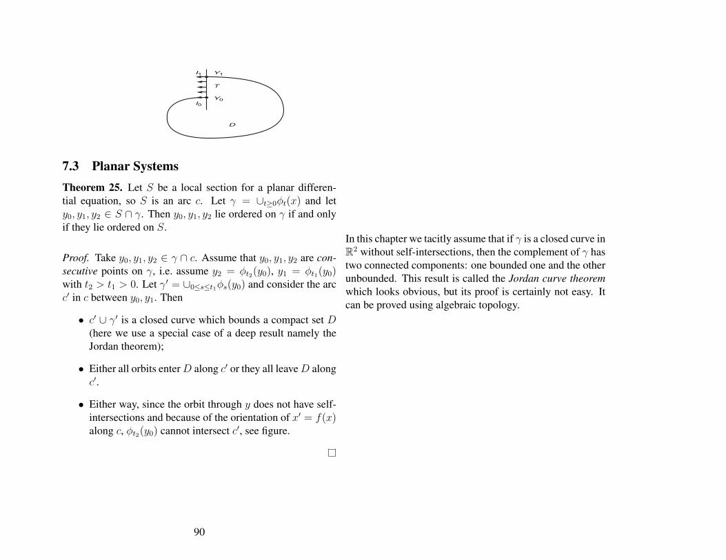
224 Chapter 10 Closed Orbits and Limit Sets

Y1

Y0I0

I1

T

D

Figure 10.7 Solutions exitthe region D through T.

Proposition. For a planar system, suppose that Y ! !(X). Then the solutionthrough Y crosses any local section at no more than one point. The same is true ifY ! "(X).

Proof: Suppose for the sake of contradiction that Y1 and Y2 are distinct pointson the solution through Y and S is a local section containing Y1 and Y2.Suppose Y ! !(X) (the argument for "(X) is similar). Then Yk ! !(X) fork = 1, 2. Let Vk be flow boxes at Yk defined by some intervals Jk " S ; weassume that J1 and J2 are disjoint as depicted in Figure 10.8. The solutionthrough X enters each Vk infinitely often; hence it crosses Jk infinitely often.

XY1

Y2

m2

m1

Figure 10.8 The solutionthrough X cannot cross V1 andV2 infinitely often.

7.3 Planar SystemsTheorem 25. Let S be a local section for a planar differen-tial equation, so S is an arc c. Let γ = ∪t≥0φt(x) and lety0, y1, y2 ∈ S ∩ γ. Then y0, y1, y2 lie ordered on γ if and onlyif they lie ordered on S.

In this chapter we tacitly assume that if γ is a closed curve inR2 without self-intersections, then the complement of γ hastwo connected components: one bounded one and the otherunbounded. This result is called the Jordan curve theoremwhich looks obvious, but its proof is certainly not easy. Itcan be proved using algebraic topology.

Proof. Take y0, y1, y2 ∈ γ ∩ c. Assume that y0, y1, y2 are con-secutive points on γ, i.e. assume y2 = φt2(y0), y1 = φt1(y0)with t2 > t1 > 0. Let γ′ = ∪0≤s≤t1φs(y0) and consider the arcc′ in c between y0, y1. Then

• c′ ∪ γ′ is a closed curve which bounds a compact set D(here we use a special case of a deep result namely theJordan theorem);

• Either all orbits enterD along c′ or they all leaveD alongc′.

• Either way, since the orbit through y does not have self-intersections and because of the orientation of x′ = f(x)along c, φt2(y0) cannot intersect c′, see figure.

90

Lemma 14. If y ∈ ω(x). Then the orbit through y intersectsany local section at most once.

Proof. 1. Assume by contradiction that y1 = φu(y) andy2 = φv(y) (where v > u) are contained on a local sec-tion S.

2. Since y ∈ ω(x) where exists tn → ∞ so that φtn(x) →y. Hence φtn+u(x)→ y1 and φtn+v(x)→ y2.

3. Since y1, y2 ∈ S, (2) implies that for n large there existsun, vn → 0 so that φtn+u+un(x) ∈ S, φtn+u+un(x) → y1

and φtn+v+vn(x) ∈ S, φtn+v+vn(x)→ y2.

4. Take n′ > n so that

tn + u+ un < tn + v + vn < tn′ + u+ vn′ . (26)

Then

φtn+u+un(x), φtn+v+vn(x), φtn′+u+vn′(x)

do not lie ordered on S: the first and last one are close toy1 and the middle one close to y2. This and (26) contra-dict the previous theorem.

91

7.4 Poincaré BendixsonTheorem 26 (Poincaré-Bendixson Theorem). Consider a pla-nar differential equation, take x ∈ R2 and assume that ω :=ω(x) is non-empty, bounded and does not contain a singularpoint of the differential equation. Then ω is a periodic orbit.

That is, we have an autonomous differential equation in R2,x = f(x) with x ∈ R2.Proof. • Assume that ω does not contain a singular point.

• Take y ∈ ω. Then there exists sm →∞ so that φsm(x)→y. Hence for each fixed t > 0, φsm+t(x) → φt(y) asm→∞. It follows that the forward orbit γ = ∪t≥0φt(y)is contained in ω. Since ω is compact, any sequenceφtn(y) has a convergent subsequence. Hence ω(y) 6= ∅and ω(y) ⊂ ω.

• Take z ∈ ω(y). Since z is not a singular point, thereexists a local section S containing z. Since z ∈ ω(y),there exists tn →∞ so that φtn(y)→ z and φtn(y) ∈ S.

• By the previous lemma, φtn(y) = φtn′ (y) for all n, n′.So ∃T > 0 so that φT (y) = y and y lies on a periodicorbit.

• We will skip the proof that ω is equal to the orbit throughy (but see lecture).

We say that A is a forward invariant domain in R2 if x ∈ Aimplies that φt(x) ∈ A for t > 0. The following theoremfollows from the previous one:

Theorem 27. Consider a planar differential equation and as-sume that A is a bounded forward invariant set so that either Adoes not contain any singularities or so that the stable manifoldeach singularity in A has dimension ≤ 1. Then A contains aperiodic orbit.

92

7.5 Consequences of Poincaré-BendixsonWe could have also restated this theorem in the followingway: Let γ be a periodic orbit of a differential equationx′ = f(x) in the plane surrounding a region D. Then Dcontains a singularity or a periodic orbit in the interior ofD.

Theorem 28. Let γ be a periodic orbit of a differential equationx′ = f(x) in the plane surrounding an open region D. Then Dcontains a singularity or another periodic orbit.

The proof is not examinable:

Proof: Assume by contradiction that D contains no othersingularity or periodic orbit. Note that the D is invariant. Takex ∈ D and consider the orbit φt(x). Then ω(x) = γ byPoincaré-Bendixson. Now consider instead of x′ = f(x) thedifferential equation x′ = −f(x) (so just run time backwards).Again γ is a periodic orbit, and applying Poincaré-Bendixsonagain, the accumulation points of φt(x) as t→ −∞ again mustbe equal to γ. Now take a section S at a point z ∈ γ. Then theprevious assertions imply that there exist sequences tn → ∞and sn → −∞ so that φtn(x), φsn(x) ∈ S. This contradictsTheorem 23 in the notes. This theorem strengthens the previous one.

Theorem 29. Let γ be a periodic orbit of a differential equa-tion x′ = f(x) in the plane surrounding a region D. Then Dcontains a singularity.

Again the proof is not examinable:

Sketch of proof: assume that D does not contain a singu-larity. Then by the previous theorem it contains another peri-odic orbit γ′. Let A ≥ 0 be the greatest lower bound of theareas of regions surrounded by periodic orbits. If A = 0 thenone can show this implies there exists a singularity. If A > 0then one can show that there exists a periodic orbit γ in Dwhich does not surround another periodic orbit. But this thencontradicts the previous lemma.

93

Other ways of proving the previous corollary are relatedto the Brouwer fixed point theorem, are rather use index argu-ments related to the Euler characteristic. To describe this oneneeds to discuss some ideas from algebraic topology.

7.6 Further Outlook• The Poincaré Bendixson theorem implies that planar dif-

ferential equations cannot have ‘chaotic’ behaviour.

• Differential equations in dimension ≥ 3 certainly canhave chaotic behaviour, see the 3rd year course dynami-cal systems (M3PA23) and for example http://www.youtube.com/watch?v=ByH8_nKD-ZM.

• To describe their statistical behaviour one uses proba-bilistic arguments; this area of mathematics is called er-godic theory. This is a 4th year course ( M4PA36). Formore information see for example, http://en.wikipedia.org/wiki/Ergodic_theory

• The geometry of attractors is often fractal like, see the3rd year course chaos and fractals (M3PA46). For moreinformation see for example, http://en.wikipedia.org/wiki/Fractal.

• Instead of differential equations one also studies discretedynamical systems, xn+1 = f(xn). When f : C → Cis a polynomial this leads to the study of Julia sets us-ing tools from complex analysis. For more information,see http://en.wikipedia.org/wiki/Julia_set.

Dynamical systems is an extremely active area, and is bothinteresting for people focusing on pure as well as those moreinterested in applied mathematics.

94

For example, Fields Medalists whose work is in or relatedto this area, include: Avilla (2014, complex dynamics), Lin-denstrauss (2010, ergodic theory), Smirnov (2010, part of hiswork relates to complex dynamics), Tao (2006, part of his workrelated to ergodic theory), McMullen (1998, complex dynam-ics), Yoccoz (1994, complex dynamics), Thurston (1982, a sig-nificant amount of work was about low and complex dynam-ics), Milnor (1962, his current work is in complex dynamics).

Applied dynamicists often aim to understand specific dy-namical phenomena, related to for example biological systems,network dynamics, stability and bifurcation issues etc.

One of the appeals of dynamical systems that it uses math-ematics from many branches of mathematics, but also that it isso relevant for applications.

95

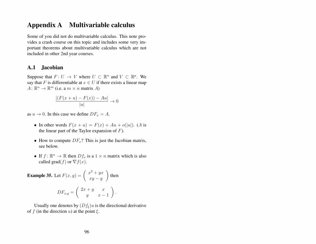
Appendix A Multivariable calculusSome of you did not do multivariable calculus. This note pro-vides a crash course on this topic and includes some very im-portant theorems about multivariable calculus which are notincluded in other 2nd year courses.

A.1 JacobianSuppose that F : U → V where U ⊂ Rn and V ⊂ Rp. Wesay that F is differentiable at x ∈ U if there exists a linear mapA : Rn → Rm (i.e. a m× n matrix A)

|(F (x+ u)− F (x))− Au||u| → 0

as u→ 0. In this case we define DFx = A.

• In other words F (x + u) = F (x) + Au + o(|u|). (A isthe linear part of the Taylor expansion of F ).

• How to compute DFx? This is just the Jacobian matrix,see below.

• If f : Rn → R then Dfx is a 1 × n matrix which is alsocalled grad(f) or∇f(x).

Example 35. Let F (x, y) =

(x2 + yxxy − y

)then

DFx,y =

(2x+ y xy x− 1

).

Usually one denotes by (Dfξ)u is the directional derivativeof f (in the direction u) at the point ξ.

96

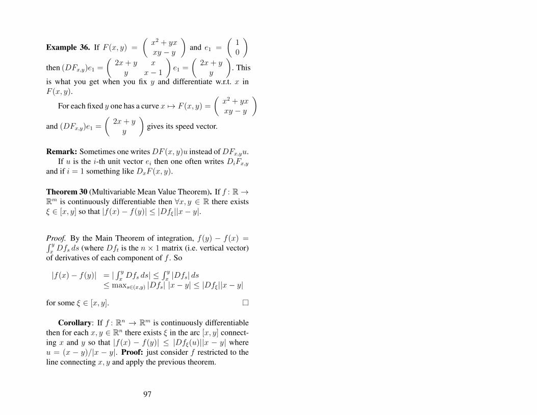
Example 36. If F (x, y) =

(x2 + yxxy − y

)and e1 =

(10

)

then (DFx,y)e1 =

(2x+ y xy x− 1

)e1 =

(2x+ yy

). This

is what you get when you fix y and differentiate w.r.t. x inF (x, y).

For each fixed y one has a curve x 7→ F (x, y) =

(x2 + yxxy − y

)

and (DFx,y)e1 =

(2x+ yy

)gives its speed vector.

Remark: Sometimes one writesDF (x, y)u instead ofDFx,yu.If u is the i-th unit vector ei then one often writes DiFx,y

and if i = 1 something like DxF (x, y).

Theorem 30 (Multivariable Mean Value Theorem). If f : R→Rm is continuously differentiable then ∀x, y ∈ R there existsξ ∈ [x, y] so that |f(x)− f(y)| ≤ |Dfξ||x− y|.

Proof. By the Main Theorem of integration, f(y) − f(x) =∫ yxDfs ds (where Dft is the n× 1 matrix (i.e. vertical vector)

of derivatives of each component of f . So

|f(x)− f(y)| = |∫ yxDfs ds| ≤

∫ yx|Dfs| ds

≤ maxs∈(x,y) |Dfs| |x− y| ≤ |Dfξ||x− y|

for some ξ ∈ [x, y].

Corollary: If f : Rn → Rm is continuously differentiablethen for each x, y ∈ Rn there exists ξ in the arc [x, y] connect-ing x and y so that |f(x) − f(y)| ≤ |Dfξ(u)||x − y| whereu = (x − y)/|x − y|. Proof: just consider f restricted to theline connecting x, y and apply the previous theorem.

97

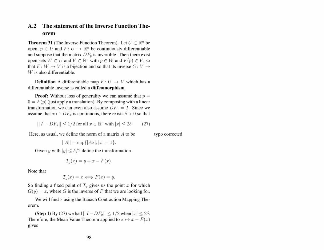
A.2 The statement of the Inverse Function The-orem

Theorem 31 (The Inverse Function Theorem). Let U ⊂ Rn beopen, p ∈ U and F : U → Rn be continuously differentiableand suppose that the matrix DFp is invertible. Then there existopen sets W ⊂ U and V ⊂ Rn with p ∈ W and F (p) ∈ V , sothat F : W → V is a bijection and so that its inverse G : V →W is also differentiable.

Definition A differentiable map F : U → V which has adifferentiable inverse is called a diffeomorphism.

Proof: Without loss of generality we can assume that p =0 = F (p) (just apply a translation). By composing with a lineartransformation we can even also assume DF0 = I . Since weassume that x 7→ DFx is continuous, there exists δ > 0 so that

|| I −DFx|| ≤ 1/2 for all x ∈ Rn with |x| ≤ 2δ. (27)

Here, as usual, we define the norm of a matrix A to be typo corrected

||A|| = sup{|Ax|; |x| = 1}.Given y with |y| ≤ δ/2 define the transformation

Ty(x) = y + x− F (x).

Note thatTy(x) = x⇐⇒ F (x) = y.

So finding a fixed point of Ty gives us the point x for whichG(y) = x, where G is the inverse of F that we are looking for.

We will find x using the Banach Contraction Mapping The-orem.

(Step 1) By (27) we had || I−DFx|| ≤ 1/2 when |x| ≤ 2δ.Therefore, the Mean Value Theorem applied to x 7→ x− F (x)gives

98

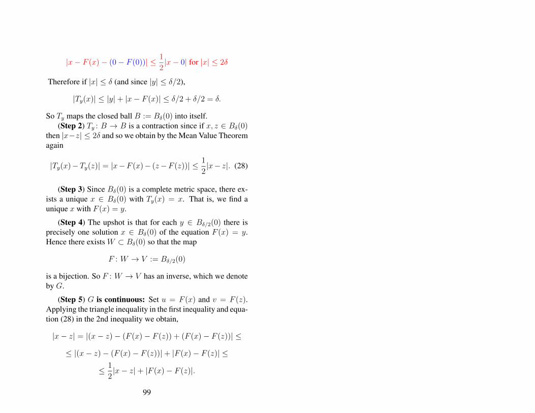
|x− F (x)− (0− F (0))| ≤ 1

2|x− 0| for |x| ≤ 2δ

Therefore if |x| ≤ δ (and since |y| ≤ δ/2),

|Ty(x)| ≤ |y|+ |x− F (x)| ≤ δ/2 + δ/2 = δ.

So Ty maps the closed ball B := Bδ(0) into itself.(Step 2) Ty : B → B is a contraction since if x, z ∈ Bδ(0)

then |x−z| ≤ 2δ and so we obtain by the Mean Value Theoremagain

|Ty(x)−Ty(z)| = |x−F (x)− (z−F (z))| ≤ 1

2|x− z|. (28)

(Step 3) Since Bδ(0) is a complete metric space, there ex-ists a unique x ∈ Bδ(0) with Ty(x) = x. That is, we find aunique x with F (x) = y.

(Step 4) The upshot is that for each y ∈ Bδ/2(0) there isprecisely one solution x ∈ Bδ(0) of the equation F (x) = y.Hence there exists W ⊂ Bδ(0) so that the map

F : W → V := Bδ/2(0)

is a bijection. So F : W → V has an inverse, which we denoteby G.

(Step 5) G is continuous: Set u = F (x) and v = F (z).Applying the triangle inequality in the first inequality and equa-tion (28) in the 2nd inequality we obtain,

|x− z| = |(x− z)− (F (x)− F (z)) + (F (x)− F (z))| ≤

≤ |(x− z)− (F (x)− F (z))|+ |F (x)− F (z)| ≤

≤ 1

2|x− z|+ |F (x)− F (z)|.

99

So |G(u)−G(v)| = |x− z| ≤ 2|F (x)− F (z)| = 2|u− v|.

(Step 6) G is differentiable:

|(G(u)−G(v))−(DFz)−1(u−v)| = |x−z−(DFz)

−1(F (x)−F (z))| ≤

||(DFz)−1||·|DFz(x−z)−(F (x)−F (z))| = o(|x−z|) = 2o(|u−v|).as ||(DFz)−1|| is bounded, using the definition and the last in-equality in step 5. Hence

|G(u)−G(v)− (DFz)−1(u− v)| = o(|u− v|)

proving that G is differentiable and that DGv = (DFz)−1.

Example 37. Consider the set of equations

x2 + y2

x= u, sin(x) + cos(y) = v.

Given (u, v) near (u0, v0) = (2, cos(1) + sin(1)) is it possibleto find a unique (x, y) near to (x0, y0) = (1, 1) satisfying thisset of equations? To check this, we define

F (x, y) =

(x2+y2

x

sin(x) + cos(y)

).

The Jacobian matrix is(

x2−y2x2

2yx

cos(x) − sin(y)

).

The determinant of this is y2−x2x2

sin(y) − 2yx

cos(x) which isnon-zero near (1, 1). So F is invertible near (1, 1) and for every(u, v) sufficiently close to (u0, v0) one can find a unique solu-tion near to (x0, y0) to this set of equations. Near (π/2, π/2)the map F is probably not invertible.

100

A.3 The Implicit Function TheoremTheorem 32 (Implicit Function Theorem). Let F : Rp×Rn →Rn be differentiable and assume that F (0, 0) = 0. More-over, assume that n × n matrix obtained by deleting the firstp columns of the matrix DF0,0 is invertible. Then there existsa function G : Rp → Rn so that for all (x, y) near (0, 0)

y = G(x)⇐⇒ F (x, y) = 0.

The proof is a fairly simple application of the inverse func-tion theorem, and won’t be given here. The Rp part in Rp×Rn

can be thought as parameters.

Example 38. Let f(x, y) = x2 +y2−1. Then one can considerthis as locally as a function y(x) when ∂f/∂y = 2y 6= 0.

Example 39. Consider the following equations:

x2 − y2 − u3 + v2 + 4 = 0,2xy + y2 − 2u2 + 3v4 + 8 = 0.

Can one write u, v as a function of x, y in a neighbourhood ofthe solution (x, y, y, v) = (2,−1, 2, 1)? To see this, define

F (x, y, u, v) = (x2−y2−u3+v2+4, 2xy+y2−2u2+3v4+8).

We have to consider the part of the Jacobian matrix which con-cerns the derivatives w.r.t. u, v at this point. That is

(−3u2 2v−4u 12v3

)∣∣∣∣(2,−1,2,1)

=

(−12 2−8 12

)

which is an invertible matrix.So locally, near (2,−1, 2, 1) one can write

(u, v) = G(x, y) that is F (x, y,G1(x, y), G2(x, y)) = 0.

101

It is even possible to determine ∂G1/∂x (i.e. ∂u/∂x). In-deed, writing u = G1(x, y) and v = G2(x, y) and differentiate:

x2 − y2 − u3 + v2 + 4 = 0,2xy + y2 − 2u2 + 3v4 + 8 = 0,

with respect to x. This gives

2x− 3u2 ∂u∂x

+ 2v ∂v∂x

= 0,2y − 4u∂u

∂x+ 12v3 ∂v

∂x= 0.

So(

∂u∂x∂v∂x

)=

(3u2 −2v4u −12v3

)−1(2x2y

)

=1

8uv − 36u2v2

(−12v3 2v−4u 3u2

)(2x2y

)

Hence∂u

∂x=

(−24xv3 + 4vy)

8uv − 36u2v2.

102

Appendix B Prerequisites

B.1 Function spaces1. Let f : [0, 1] → R be a function and fn : [0, 1] → R be

a sequence functions. Define what it means to say thatfn → f uniformly.

Answer: for all ε > 0 there exists n0 so that for all n ≥n0 and all x ∈ [0, 1] one has |fn(x)− f(x)| < ε.

Answer 2: ||fn − f ||∞ → 0 as n → ∞ where ||fn −f ||∞ = supx∈[0,1] |fn(x)− f(x)|.

2. Let f : [0, 1] → R be a function and fn : [0, 1] → R bea sequence functions. Define what it means to say thatfn → f pointwise.

Answer: for all ε > 0 and all x ∈ [0, 1] there exists n0 sothat for all n ≥ n0 one has |fn(x)− f(x)| < ε.

3. Let f : [0, 1] → R be a function and fn : [0, 1] → R be asequence functions. Assume that fn → f uniformly andthat fn is continuous. Show that f is continuous.

Answer: Take ε > 0, x ∈ [0, 1]. Choose n0 so that|fn − f |∞ < ε/3 for n ≥ n0 and pick δ > 0 so that|fn0(x)− fn0(y)| < ε/3 for all y with |y − x| < δ. Thenfor all y with |y − x| < δ, |f(x) − f(y)| < |f(x) −fn0(x)| + |fn0(x) − fn0(y)| + fn0(y) − f(y)| < ε/3 +ε/3 + ε/3 = ε.

4. Let f : [0, 1] → R be a function and fn : [0, 1] → R bea sequence functions. Assume that fn → f pointwiseand that fn is continuous. Show that f is not necessarilycontinuous.

Answer: Take fn(x) = (1 − nx) for x ∈ [0, 1/n] andfn(x) = 0 elsewhere. Then fn → f pointwise, where

103

f(0) = 1 and f(x) = 0 for x ∈ (0, 1].

Appendix C Explicit methods for solv-ing ODE’s

This Appendix summarises explicit methods for solving ODE’s.Since most of the material is already covered in first year ma-terial, it will not be covered in the lectures.

C.1 State independent• This section summarises techniques for solving ODE’s.

• The first subsections are about finding x : R→ R so thatx′ = f(x, t) and x(0) = x0 where f : R2 → R.

• So the issue is to find curves with prescribed tangents.

• Let us first review methods for explicitly solving suchequations (in part reviewing what you already know).

C.2 State independent x = f(t).

In this case, each solution is of the form x(t) =∫ t

0f(s) ds +

x(0).

Example 40. Assume the graph t 7→ (t, x(t)) has tangentvector (1, sin(t)) at t. Then x′(t) = sin(t) and so x(t) =− cos(t) + c. So the solution of the ODE x′(t) = sin(t) finds acurve which is tangent to the arrows of the vector field.

104

C.3 Separation of variablesSeparation of variables: x = f(t)g(x). Then one can findsolutions as follows.

∫ x(T )

x(0)

dy

g(y)=

∫ T

0

1

g(x(t))

dx

dtdt =

∫ T

0

f(t) dt.

Here the first equality follows from the substitution rule (takingy = x(t)) and 2nd from 1

g(x(t))dxdt

= f(t).

Example 41. dxdt

= ax+ b, x(t) = x0. Then dxax+b

= dt, x(0) =x0 which gives, when a 6= 0,

(1/a)[log(ax+ b)]x(T )x0

= T,

log((ax(T ) + b)/(ax0 + b)) = aT

and therefore

x(T ) = x0eaT +

eaT − 1

ab for T ∈ (−∞,∞)

Example 42. dxdt

= x2, x(0) = x0. Then dxx2

= dt, x(0) = x0.Hence [−1/x]

x(t)x0 = t and so x(t) = 1

1/x0−t . Note that x(t)

is well-defined for t ∈ (−∞, 1/x0) but that x(t) → ∞ ast ↑ 1/x0. The solution goes to infinity in finite time.

Example 43. dxdt

=√|x|, x(0) = x0. If x0 > 0 and x(t) > 0

then we obtain dx√x

= dt, x(0) = x0 and so 2√x(t)− 2

√x0 =

t. Thus x(t) = (√x0 + t/2)2 for t ∈ (−2

√x0,∞). When

t = −2√x0 then x(t) = 0, so need to analyse this directly.

When x0 = 0 then there are many solutions (non-uniqueness).For any −∞ ≤ t0 ≤ 0 ≤ t1 ≤ ∞

x(t) =

−(t− t0)2/4 for t ∈ (−∞, t0)

0 for t ∈ [t0, t1](t− t1)2/4 for t ∈ (t1,∞)

is a solution.

105

So, without imposing some assumptions, solutions neednot be unique.

C.4 Linear equations x′ + a(t)x = b(t).To solve this, first consider the homogeneous case x′+a(t)x =0. This can be solved by separation of variables: dx/x=-a(t)dtand so x(t) = x0 exp[−

∫ t0a(s) ds].

To find the solution of the ODE, apply the variation of vari-ables ‘trick’: substitute x(t) = c(t) exp[−

∫ t0a(s) ds] in the

equation and obtain an equation for c(t).

Example 44. x′ + 2tx = t. The homogeneous equation x′ +2tx = 0 has solution x(t) = ce−t

2 .Substituting x(t) = c(t)e−t

2 into x′+2tx = t gives c′(t)e−t2+c(t)(−2t)e−t

2+ 2tc(t)e−2t2 = t, i.e. c′(t) = tet

2 . Hencec(t) = c0 + (1/2)et

2 and therefore x(t) = c0e−t2 + (1/2).

That the equation is of the form

c0 · solution of hom.eq + special solution

is due to the fact that the space of solutions x′ + 2tx = 0 islinear (linear combination of solutions are again solutions).

C.5 Exact equationsM(x, y)dx+N(x, y)dy = 0when ∂M/∂y = ∂N/∂x.

Suppose f(x, y) ≡ c is a solution. Then df = (∂f/∂x)dx +(∂f/∂y)dy = 0 and this corresponds to the ODE if ∂f/∂x =M and ∂f/∂y = N . But if f is twice differentiable we have

∂M/∂y = ∂2f/∂x∂y = ∂2f/∂y∂x = ∂N/∂x.

It turns out that this necessary condition for ‘exactness’ is alsosufficient if the domain we consider has no holes (is simplyconnected).

106

Example 45. (y − x3)dx + (x + y2)dy = 0. The exactnesscondition is satisfied (check!). How to find f with ∂f/∂x =y−x3 and ∂f/∂y = x+y2? The first equation gives f(x, y) =yx−(1/4)x4+c(y). The second equation then gives x+c′(y) =∂f/∂y = x + y2. Hence c(y) = y3/3 + c0 and f(x) = yx −(1/4)x4 + y3/3 + c0 is a solution.

Sometimes you can rewrite the equation to make it exact.

Example 46. ydx + (x2y − x)dy = 0. This equation is not

exact (indeed,∂y

∂y6= ∂(x2y − x)

∂x). If we rewrite the equation

as y/x2dx+ (y − 1/x)dy = 0 then it becomes exact.

Clearly this was a lucky guess. Sometimes one can guessthat by multiplying by a function of (for example) x the ODEbecomes exact.

Example 47. The equation (xy−1)dx+(x2−xy)dy = 0 is notexact. Let us consider the equation µ(x)(xy−1)dx+µ(x)(x2−xy)dy = 0. The exactness condition is µx = µ′(x2 − xy) +µ(2x−y). Rewriting this gives µ′(x)x(x−y)+µ(x)(x−y) = 0,and so xµ′+µ = 0 implies the exactness condition. So we cantake µ(x) = 1/x. So instead of the original ODE we solve(y − 1/x)dx+ (x− y)dy = 0 as in the previous example.

C.6 Substitutions• Sometimes one can simplify the ODE by a substitution.

• One instance of this method, is when the ODE is of theform M(x, y)dx + N(x, y)dy = 0 where M,N are ho-mogeneous polynomials of the same degree.

In this case we can simplify by substituting z = y/x.

107

Example 48. (x2 − 2y2)dx+ xydy = 0. Rewrite this as dydx

=−x2+2y2

xy. Substituting z = y/x, i.e. y(x) = z(x)x gives

xdz

dx+ z =

dy

dx=−1 + 2z2

z.

Hencedz

dx=−1

z+ z.

This can be solved by separation of variables.

C.7 Higher order linear ODE’s with constantcoefficients

Note that each y1 and y2 are solutions of

y(n) + an−1y(n−1) + · · ·+ a0y = 0 (29)

then linear combinations of y1 and y2 are also solutions.Substituting y(x) = erx in this equation gives:

ern(rn + an−1r

n−1 + · · ·+ a0

)= 0.

Of course the polynomial equation rn+an−1rn−1+· · ·+a0 = 0

has n solutions r1, . . . , rn ∈ C.

Case 1: If these ri’s are all different (i.e. occur with singlemultiplicity), then we obtain as a solution:

y(x) = c1er1x + · · ·+ cne

rnx.

Case 2: What if, say, r1 is complex? Then r1 is also aroot, so we may (by renumbering) assume r2 = r1 and writer1 = α + βi and r2 = α− βi with α, β ∈ R. So

er1x = eαx(cos(βx)+sin(βx)i), er2x = eαx(cos(βx)−sin(βx)i),

108

and c1er1x+c2e

r2x = (c1+c2)eαx cos(βx)+(c1−c2)ieαx sin(β).Taking c1 = c2 = A/2 ∈ R =⇒ c1e

r1x + c2er2x =

Aeαx cos(βx) On the other hand, taking c1 = −(B/2)i =−c2 =⇒ c1e

r1x + c2er2x = Beαx sin(βx) (nothing prevents

us choosing ci non-real!!).

So if r1 = r2 is non-real, we obtain as a general solution

y(x) = Aeαx cos(βx) +Beαx sin(βx) + c3er3x + · · ·+ cne

rnx.

Case 3: Repeated roots: If r1 = r2 = · · · = rk then onecan check that c1e

r1x + c2xer2x + · · ·+ ckx

ker1x is a solution.

Case 4: Repeated complex roots: If r1 = r2 = · · · =rk = α + βi are non-real, then we have corresponding rootsrk+1 = rk+2 = · · · = r2k = α− βi and we obtain as solution

c1eαx cos(βx) + · · ·+ ckx

keαx cos(βx)+

+ck+1eαx sin(βx) + · · ·+ c2kx

keαx sin(βx).

Example 49. Vibriations and oscillations of a springOne can model an object attached to a spring by Mx′′ =

Fs + Fd where Fd is a damping force and Fs a spring force.Usually one assumes Fd = −cx′ and Fs = −kx. So

Mx′′ + cx′ + kx = 0 or x′′ + 2bx′ + a2x = 0

where a =√k/M > 0 and b = c/(2M) > 0.

Using the previous approach we solve r2 + 2br + a2, i.e.r1, r2 = −2b±

√4b2−4a2

2= −b±

√b2 − a2.

Case 1: If b2−a2 > 0 then both roots are real and negative.So x(t) = x0(er1t + Ber2t) is a solution and as t → ∞ we getx(t)→ 0.

Case 2: If b2 − a2 = 0 then we obtain r1 = r2 = −a andx(t) = Ae−at +Bte−at. So x(t) still goes to zero as→∞, butwhen B is large, x(t) can still grow for t not too large.

109

Case 3: If b2 − a2 < 0. Then x(t) = e−bt(A cos(αt) +B sin(αt)) is a solution. Solutions go to zero as t → ∞ butoscillate.

Example 50. Vibriations and oscillations of a spring withforcing

Suppose one has external forcing

Mx′′ + cx′ + kx = F0 cos(ωt).

If b2−a2 < 0 (using the notation of the previous example) then

e−bt(A cos(αt) +B sin(αt))

is still the solution of the homogeneous part and one can check

F0√(k − ω2M)2 + ω2c2

(ωc sin(ωt) + (k − ω2M) cos(ωt) =

F0√(k − ω2M)2 + ω2c2

cos(ωt− φ)

is a particular solution where ω = arctan(ωc/(k − ω2M)).

F0√(k − ω2M)2 + ω2c2

cos(ωt− φ)

is a particular solution where ω = arctan(ωc/(k − ω2M)).Here c is the damping, M is the mass and k is the spring

constant.

• If damping c ≈ 0 and ω ≈ k/M then the denominator islarge, and the oscillation has large amplitude.

• (k − ω2M)2 + ω2c2 is minimal for ω =

√k

M− c2

2M2

and so this is the natural frequency (or eigen-frequency).

110

Figure 5: The vector field (1, sin(t)) drawn with the Maplecommand: with(plots):fieldplot([1, sin(t)], t = -1 .. 1, x = -1 ..1, grid = [20, 20], color = red, arrows = SLIM);

• This is important for bridge designs (etc), see

– http://www.ketchum.org/bridgecollapse.html

– http://www.youtube.com/watch?v=3mclp9QmCGs

– http://www.youtube.com/watch?v=gQK21572oSU

C.8 Solving ODE’s with mapleExample 51. > ode1 := diff(x(t), t) = x(t)^2;

d 2--- x(t) = x(t)dt

> dsolve(ode1);1

x(t) = ---------t + _C1

> dsolve({ode1, x(0) = 1});1

x(t) = - -----t - 1

Example 52. Example: y′′ + 1 = 0.

111

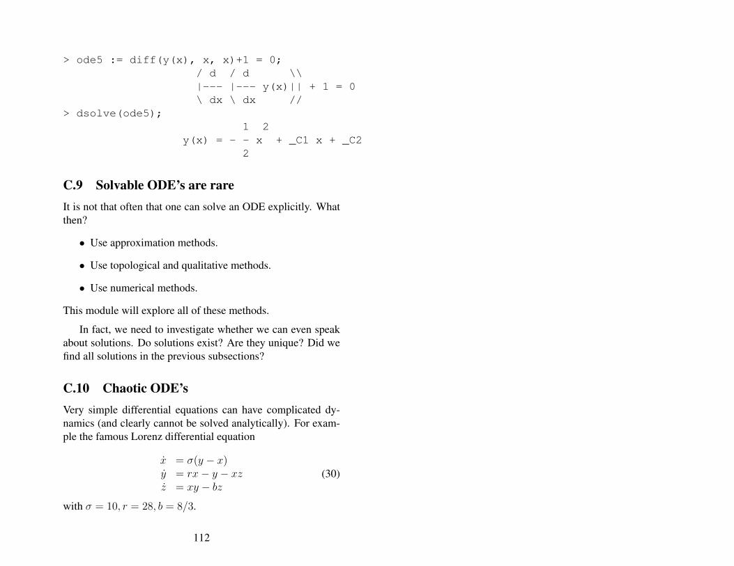
> ode5 := diff(y(x), x, x)+1 = 0;/ d / d \\|--- |--- y(x)|| + 1 = 0\ dx \ dx //

> dsolve(ode5);1 2

y(x) = - - x + _C1 x + _C22

C.9 Solvable ODE’s are rareIt is not that often that one can solve an ODE explicitly. Whatthen?

• Use approximation methods.

• Use topological and qualitative methods.

• Use numerical methods.

This module will explore all of these methods.

In fact, we need to investigate whether we can even speakabout solutions. Do solutions exist? Are they unique? Did wefind all solutions in the previous subsections?

C.10 Chaotic ODE’sVery simple differential equations can have complicated dy-namics (and clearly cannot be solved analytically). For exam-ple the famous Lorenz differential equation

x = σ(y − x)y = rx− y − xzz = xy − bz

(30)

with σ = 10, r = 28, b = 8/3.

112

has solutions which are chaotic and have sensitive depen-dence (the butterfly effect).

http://www.youtube.com/watch?v=ByH8_nKD-ZM

Appendix D A proof of the Jordan nor-mal form theorem

In this section we will give a proof of the Jordan normal formtheorem.

Lemma 15. Let L1, L2 : V → V where V is a finite dimen-sional vector space. AssumeL1L2 = 0 and ker(L1)∩ker(L2) ={0}. Then V = ker(L1)⊕ ker(L2).

Proof. Let n be the dimension of V and let =(L2) stands forthe range of L2. Note that dim ker(L2) + dim=(L2) = n,Since L1L2 = 0 it follows that ker(L1) ⊃ =(L2) and thereforedim ker(L1) ≥ dim=(L2) = n − dim ker(L2). As ker(L1) ∩ker(L2) = {0}, equality holds in dim ker(L1)+dim ker(L2) ≥n and the lemma follows.

Proposition 1. Let L : V → V where V is a finite dimensionalvector space. Let λ1, . . . , λs be its eigenvalues with (algebraic)multiplicity mi. Then one can write V = V1 ⊕ V2 ⊕ · · · ⊕ Vswhere Vi = ker((L− λiI)mi) and so L(Vi) ⊂ Vi.

Proof. Consider the polynomial p(t) = det(tI − L). This is apolynomial of degree n, where n is the dimension of the vectorspace and with leading term tn. By the Cayley-Hamilton the-orem one has p(L) = 0 and of course p(L) is also of the formLn + c1L

n−1 + · · ·+ cn = 0. This can be factorised as

(L− λ1I)m1(L− λ2I)m2 · · · (L− λsI)ms = 0,

where all λi’s are distinct - here we use that the factors (L−λiI)commute.

113

We claim that ker((L − λiI)mi) ∩ ker(L − λjI)mj = 0.Indeed, if not then we can take a vector v 6= 0 which is in theintersection. We may assume mi ≥ mj . Choose 1 ≤ m′j ≤ mj

minimal so that (L − λjI)m′jv = 0 and (L − λjI)m

′j−1v 6=

0. Since v ∈ ker((L − λiI)mi) we have that w := (L −λjI)m

′j−1(L− λiI)miv is equal to 0, but on the other hand w is

equal to (L− λjI)m′j−1((L− λjI) + (λj − λi))miv which, by

expanding the latter expression (and using that v ∈ ker((L −λiI)mi)) is equal to (L − λjI)m

′j−1(λj − λi)

miv 6= 0. Thiscontradiction proves the claim.

This means that we can apply the previous lemma induc-tively to the factors (L − λiI)mi , and thus obtain the proposi-tion.

It follows that if we choose T so that it sends the decom-position Rn1 ⊕ . . .Rnk , where ni = dimVi, to V1 ⊕ · · · ⊕ Vk

then T−1LT is of the form

A1

. . .Ap

where Ai are

square matrices corresponding to Vi (and the remaining entriesare zero). The next theorem gives a way to find a more precisedescription for a linear transformation T so that T−1LT takesthe Jordan form. Indeed, we apply the next theorem to eachmatrix Ai separately. In other words, for each choice of i, wetake W = Vi, A = (L − λiI)|Vi and m = mi in the theorembelow.

Theorem 33. Let A : W → W be a linear transformation ofa finite dimensional vector space so that Am = 0 for somem ≥ 1. Then there exists a basis W of the form

u1, Au1, . . . , Aa1−1u1, . . . , us, . . . , A

as−1(us)

where ai ≥ 1 and Aai(ui) = 0 for 1 ≤ i ≤ s.

114

Remark: Note thatAaj−1(uj) = (T−λi)aj−1(uj) is in the ker-nel of A = T −λiI , so is an eigenvector of A corresponding toeigenvalues 0 (i.e. an eigenvector of T corresponding to eigen-value λi. The vector w1

j = Aaj−2(uj) = (T−λiI)aj−2(uj) cor-responds to a vector so that Aw1

j = wj , so Tw1j = λw1

j + wj ,and so on. So as in Chapter 2, if we take the matrix T withcolumns

Aa1−1u1, . . . , u1, Aa2−1u2, . . . , u2, A

as−1us, . . . , us

then T−1LT will have the required Jordan form with λ on thediagonal, and 1’s in the off-diagonal except in columns a1, a1 +a2, . . . , a1 + a2 + · · ·+ as.

Proof. The proof given below goes by induction with respectto the dimension of W . When dimW = 0 the statement isobvious. Assume that the statement holds for dimensions <dim(W ). Note that A(W ) 6= W since otherwise AW = Wand therefore Am(W ) = Am−1(W ) = · · · = W which is acontradiction. So dimA(W ) < dimW and by induction thereexists v1, . . . , vl ∈ A(W ) so that

v1, Av1, . . . , Ab1−1(v1), . . . , vl, Avl, . . . , A

bl−1vl (31)

is a basis for A(W ) and Abi(vi) = 0 for 1 ≤ i ≤ l. Sincevi ∈ A(W ) one can choose ui so that Aui = vi. The vec-torsAb1−1v1, . . . , A

bl−1vl are linearly independent and are con-tained in ker(A) and so we can find vectors ul+1, . . . , um sothat

Ab1−1v1, . . . , Abl−1vl, ul+1, . . . , um (32)

forms a basis of ker(A). But then

u1, Au1, . . . , Ab1(u1), . . . , ul, . . . , A

blul, ul+1, . . . , um (33)

is the required basis of W . Indeed, consider a linear combina-tion of vectors from (33) and applyA. Then, because vi = Aui,

115

we obtain a linear combination of the vectors from (31) and sothe corresponding coefficients are zero. The remaining vec-tors are in the kernel of A and are linearly independent becausethey correspond to (32). This proves the linear independenceof (33). That (33) spans W holds, because the number of vec-tors appearing in (33) is equal to dim ker(A) + dimAW . In-deed, Ab1(u1), . . . , Ablul, ul+1, . . . , um are all in ker(A) (theyare the same vectors as the vectors appearing in (32)). The re-maining number of vectors is b1 + · · · + bl which is the sameas the dimension of AW , as (31) forms a basis of this space.It follows that the total number of vectors in (33) is the sameas dim(ker(A)) + dim(AW ) and so together with their linearindependence this implies that (33) forms a basis of W .

116