From Van der Meer scans to precision cross section

determination: the CMS luminosity and W/Z cross section

measurements at √s=8 TeV

1

M. Zanetti (MIT) on behalf of the CMS collaboration

Overview

2

Overview

3

Overview

4

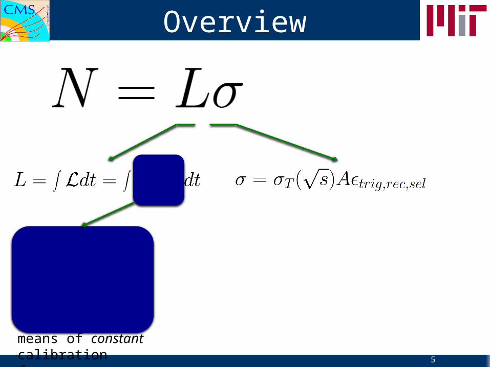
The target physics quantity (inclusive)

Overview

5

Luminosity analysis: convert rates into instantaneous luminosity by means of constant calibration factor

Overview

6

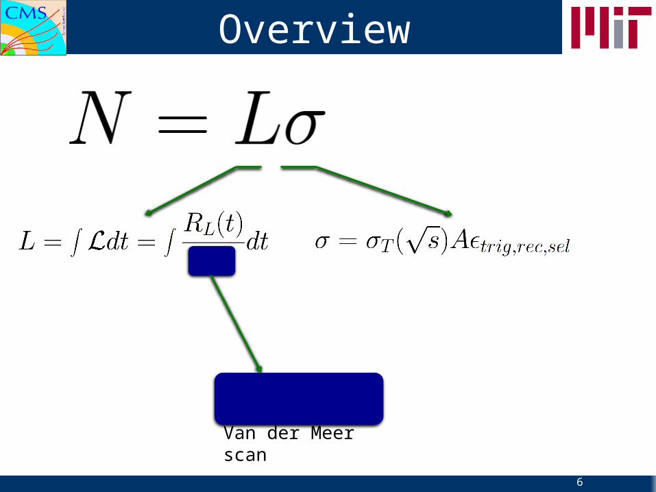
Absolute calibration: Van der Meer scan

Overview

7

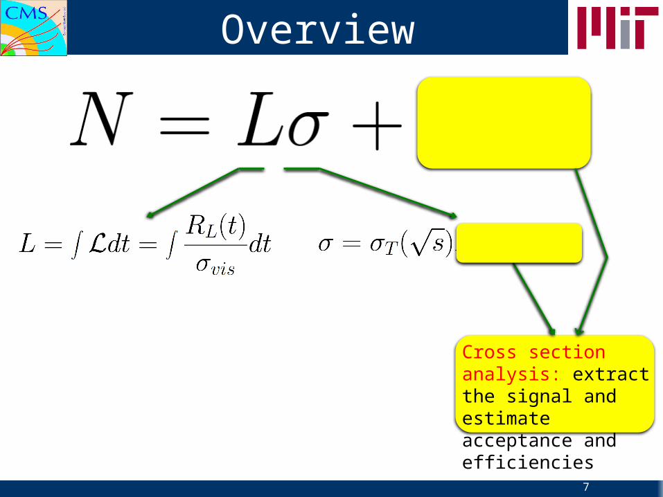
Cross section analysis: extract the signal and estimate acceptance and efficiencies

Overview

8

Cross section analysis: extract the signal and estimate the efficiencies

The target physics quantity (fiducial)

Overview

9

Wenninger, J., “Energy Calibration of the LHC Beams at 4 TeV” CERN-ATS-2013-040

Luminosity calibration(determination of svis)

10

Disclaimer / acknowledgementsMost of the aspects discussed in the following have profited from the work and the collective effort of the “Bunch Currents Normalization” and “LHC Luminosity Calibration and Monitor” working groups that gathered experts from the machine and the LHC experiments

11

• The (per BX) instantaneous lumi is a complicated function of beam parameters:

• Beam measurements during physics runs not accurate enough (~10-20%)

• Exploit R=Ls relation:– s from a very accurately predicted physics process that can be very

well isolated experimentally (physics candles)• Bhabha scattering at LEP• Zmm at LHC (hum, wait a moment..)

– Perform dedicated experiment to measure L from beam parameters Van der Meer scan

• Note that in both cases s is required to be constant!

Measuring luminosity

12

€

L = υN1N2

r v 1 −

r v 2( )

2−

r v 1 ×

r v 2( )

2

c 2ρ1

lab r r − Δ

r r , t( )ρ 2

lab r r , t( )d3r

r dt∫

€

L =υ N1N2

2π σ 1,x2 + σ 2,x

2( ) σ 1,y

2 + σ 2,y2

( )

Gaussian beams

• Goal is to determine luminosity from beam parameters– Beam current measured by dedicated beam instrumentation

• DC Beam Current Transformer: total circulating charges• Fast Beam Current Transformer: fraction of charge in each bunch

– “Affective area” assessed from rate as a function of beam separation

• Van der Meer technique, i.e. determine “effective height” of the beams (S):

– With F(D) implementing the dependency on separation, the luminosity is defined as:

Measuring beam parameters

13

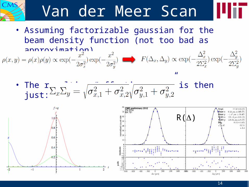
• Assuming factorizable gaussian for the beam density function (not too bad as approximation)

• The resulting “effective area” is then just:

Van der Meer Scan

14

R(D)

• Scan the beams horizontally and vertically– In steps of half beam width, ~25 steps, ~30 sec per step,

• Dedicated beam/machine set up (time consuming!)– Reduced number of bunches, reduced bunch intensity– Larger b*, no crossing angle

• Conditions further and further optimized– Excellent results from last scan at √s=8TeV, Nov. 2012

• H. Bartosik, G. Rumolo, CERN-ACC-NOTE-2013-0008– Aim at maximize validity of assumptions (factorizability and Gaussian shape)

Van der Meer Scans at LHC

15

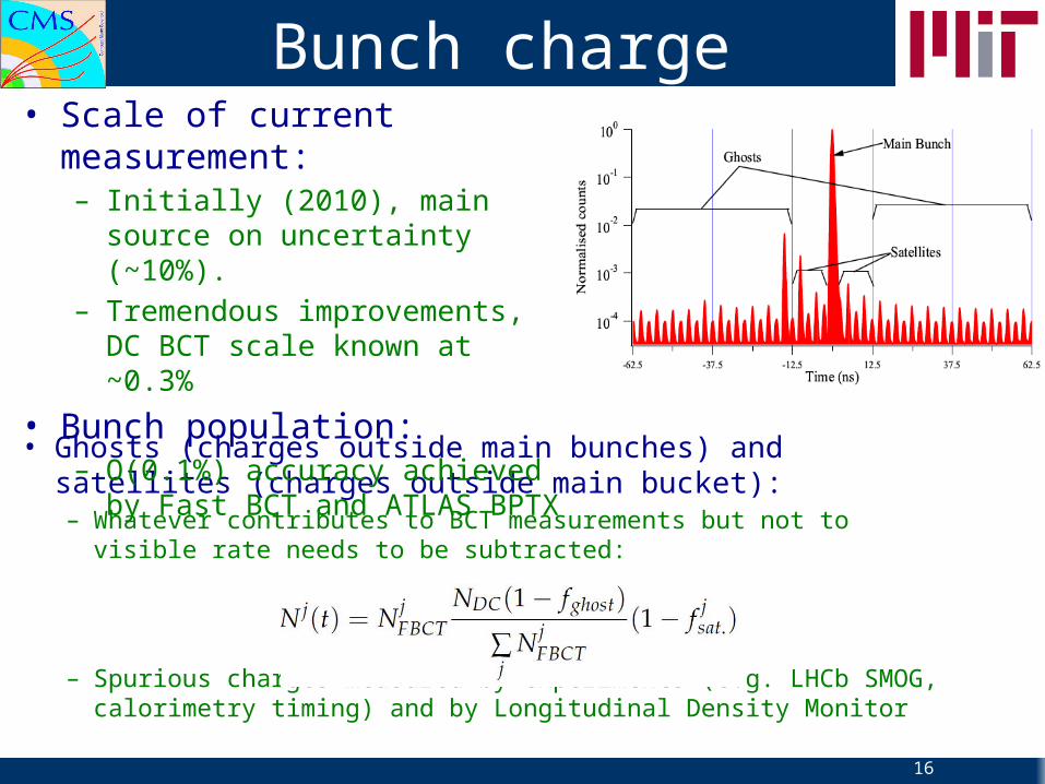
• Ghosts (charges outside main bunches) and satellites (charges outside main bucket):– Whatever contributes to BCT measurements but not to visible rate

needs to be subtracted:

– Spurious charges measured by experiments (e.g. LHCb SMOG, calorimetry timing) and by Longitudinal Density Monitor

Bunch charge

16

• Scale of current measurement:– Initially (2010), main source on

uncertainty (~10%). – Tremendous improvements, DC BCT

scale known at ~0.3%

• Bunch population: – O(0.1%) accuracy achieved by Fast

BCT and ATLAS BPTX

• Length scale– Value of the separation derived from

currents in the corrector magnets– This is calibrated against central tracking

system– Compare luminous region information

(vertices distribution) versus nominal sep.

• Emittance growth– Beams size are known to increase in size

during the fill. – Effect is sizable during the ~30 minutes– Bias almost negligible if emittance grows

linearly with time and if measurement are made in between X and Y scans

Corrections to VdM analysis

17

• Orbit drift– The beams can slowly drift in the

transverse plane; effect is typically small but can be harmful in some cases

– Drift of the orbit estimated by BPM measurements taken between scans and extrapolated to IP

Corrections to VdM analysis

18

• Beam-beam effects:– Dipolar kick (beam-beam deflection):

• Repulsive force deflects beams affecting nominal separation

• depends on the separation itself, the beam width and the current

– Quadrupolar (de)focusing (dynamic b):• Effective beam width modified depending on

the separation• Peak luminosity (rate) affected

T. Pieloni, W. Kozanecki

• It is convenient to take the assumption that the beam density functions can be factorized– E.g. the scan is performed separately along X and Y

• The Van der Meer method works for whatever shape F(Dx,Dx), but that shape needs to be known.– Best would be to deal with (single) gaussian distribution

• Several observations indicating that is not the case if no adequate preparation of the beam/machine setup– Luminous region behavior, scan to scan variation of calibration

Gaussian and Factorizable?

19

Lumi Region X width during Y scan

svisApril 2012 VdM scans April 2012 VdM scans

• If beams/machine(s) are prepared such that densities are good single gaussian (Nov 2012), non-linearity and non-factorizability effects are very much reduced

• The exact functional form is however still unknown major source of uncertainty– A full bias study (based on Monte Carlo) is needed

Gaussian and Factorizable?

20

Lumi Region X width during Y scan

Nov 2012 VdM scans C. Barshel, LHCb beam gas analysis

Luminosity integration

21

• As for any other cross section:

• Acceptance and efficiencies may depend on many things:– Acceptance: detector conditions (alive channels), beam positions, etc.– Efficiency: detector setup, pileup, filling scheme, etc.

• A perfect luminometer is a device that measures rates with constant acceptance and efficiency

• Any real implementation requires corrections– What to use as a reference?

Ideal Luminometer

22

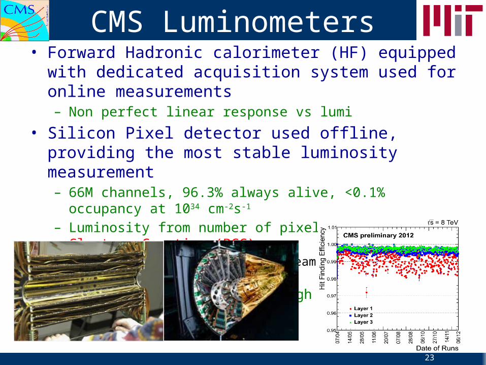
• Forward Hadronic calorimeter (HF) equipped with dedicated acquisition system used for online measurements– Non perfect linear response vs lumi

• Silicon Pixel detector used offline, providing the most stable luminosity measurement– 66M channels, 96.3% always alive, <0.1% occupancy at 1034 cm-2s-1

– Luminosity from number of pixel clusters, Pixel Clusters Counting (PCC)• Dedicated high rate data stream triggering on Zero Bias

– Linear response till very high pileup (1% of shared clusters at m=200)

CMS Luminometers

23

• Acceptance:– Restrict set of channels to those always

alive throughout the running period– Beam jitter small enough not to affect

geometrical acceptance

• Efficiencies:– Online and offline threshold such that

signal efficiency insensitive to recalibration (needed to compensate effects of radiation dose)

– Dynamic inefficiencies: filling up of the read-out buffer busy state for DAQ loss of efficiency. Dependency on trigger rate luminosity

PCC: Dependencies

24

• Being the reference in terms of stability, it can only be compared with itself

• The figure of merit is relative contributions of detector components are compared– Fractions are stable at the 0.5% level– Some collective effects can be hidden (rather unlikely)

• Alternatively compare to Z->mm rates (study ongoing)

PCC: Stability check

25

2012 pp run

• “Out of time response” featured by the cluster counting method:– Pulse shape: not relevant for 50 ns scheme, will it be at 25 ns?– Mild activation of the surrounding material

• Try to model and estimate the single bunch response assuming an exponential decay– Does not depend on the filling scheme

• Small contribution which however sums up to a non negligible component in highly populated filling schemes, ~2% effect

PCC: Afterglow

26

Luminosity Uncertainties

27

Statistical error from rate profile fit, ~0.5%

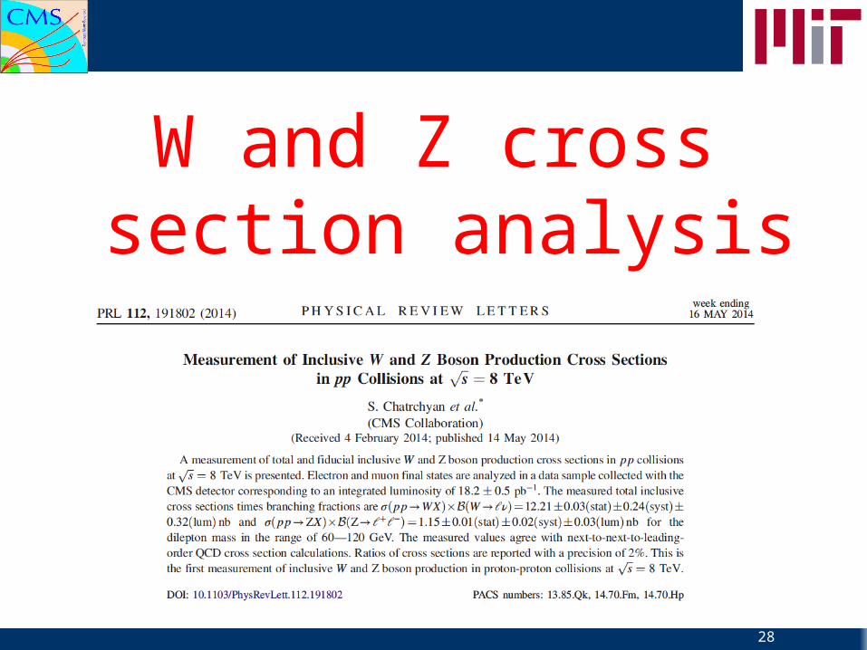
W and Z cross section analysis

28

• One of the most important measurements in 2010 (7TeV, 35/pb)• Run at 8 TeV in much harsher conditions (PU x10, L x30)

– E.g. single lepton L1 trigger rate >>100kHz if same thresholds as in 2010– Larger uncertainties in modeling MET

• Analysis is systematically limited can tradeoff dataset size for better conditions

• Low Luminosity run yielding a dataset of ~20/pb:– During intensity ramp-up (minimizing loss of integrated luminosity),

separate the beams and level pilup at ~5– Allow lowering L1 thresholds on single lepton pT – Dedicated high rate HLT configuration (~300Hz for single lepton triggers)

• Basically identical analysis as in 2010 is allowed

Dedicated data taking

29

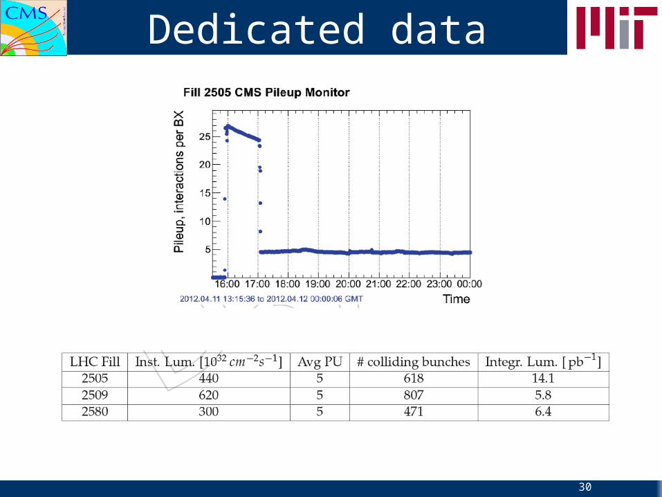
Dedicated data taking

30

Quite a useful dataset indeed!

Dedicated data taking

31

• Both W and Z analysis rely on single lepton triggers:

• Offline selections– Electrons

• pT>25 GeV; |h|<1.44, 1.57<|h|<2.5

• isolation: SpTi<0.15pT

ele (sum over Particle Flow candidates in cone DR=0.3)

– Muons• pT>25 GeV; |h|<2.1

• isolation: SpTi<0.12pT

m (sum over Particle Flow candidates in cone DR=0.4)

– W selections:• No MET cut, use MET to discriminate signal and background• MET as computed by Particle Flow reconstruction, modeled by recoil method

– Z selections:• 60<mll<120 GeV

Selection

32

• Mainly affecting W analysis • QCD:

– Multi-jet or high Et photon (electron channels)– Assessed by fully data driven techniques

• Electroweak:– Drell-Yan (one lepton missing).

• Veto applied small contribution– Leptonic decays of taus (Wtn, Ztt)

• pT requirement on leptons suppresses it

– Top and di-bosons (very small)– Use Monte Carlo to describe the shape, normalization bound to W

cross section according to theoretical predictions

Backgrounds

33

• Acceptance is estimated from simulation, corrected for efficiency

• No Monte Carlo generator combines optimal EWK and QCD predictions. Use POWHEG/CT10 for central value

• Other tools are used to estimate systematic uncertainties– Non perturbative QCD effects-> Resbos (NNLL)– Missing higher order QCD corrections -> scale variation with FEWZ– EWK corrections: HORACE

• PDF (dominant effect): – Uncertainty from nominal PDF set (CT10)

Acceptance

34

• Main source of experimental uncertainties• Tag&Probe method:

– Tight id/isolation for the tag lepton that gives the Z mass together with a second lepton, the latter being an unbiased probe to the efficiency

– Fit to the mass spectrum in case on non negligible background

• Efficiency is factorized, each estimated w.r.t to previous selection • (h,pT) dependent scale factors are obtained and used to

compensate differences between data and MC• Systematic uncertainties computed by exploiting different models

for signal and background– Signal: MC shape*Gaussian (default), Breit-Wigner*Cyrstal-Ball– Bkgr: Exponential (default), linear, ErrF*Exp, MC template from W+jets+QCD– N.B. statistic of the tag&probe sample affects systematic error

Efficiencies

35

• Perform fit to MET distribution to distinguish signal over background

• Accurate MET model obtained by “recoil method”– Remove leptons from Z boson data and estimate recoil components

(perpendicular and parallel to the boson pT) vs the boson pT– Data and MC are compared, corrections are applied to W simulation

• EWK bkgr at ~6% level for both e and m• QCD background is modeled by Rayleigh function

– Electrons (good S-B discrimination): s0 and s1 left free in the fit– Muons: simultaneous fit of signal and control region (inverse isolation)

both constraining the tail parameter (s1)

– Systematics assessed by adding an extra shape parameter (s2), and different definitions of control regions (muon isolation)

W Signal Extraction

36

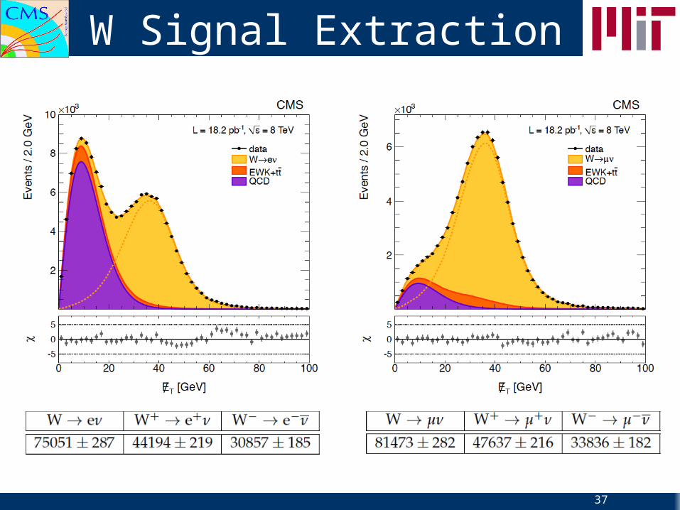
W Signal Extraction

37

• Tiny background (0.4%), estimated from simulation• Events yields computed by counting events in the mass window• Systematics assessed by comparing simultaneous fit approach

(cfr. 7 TeV analysis)

Z Signal Extraction

38

• Estimation of uncertainties follows closely what done in the 7 TeV analysis

• Some errors (most importantly luminosity) cancels in the ratios. Lepton efficiencies are however considered as uncorrelated (can be larger than individual measurements)

Systematic Uncertainties

39

• Theoretical predictions from FEWZ and MSTW2008 PDF set– Uncertainties come from as, heavy quark masses, and missing high orders

• Results in muon and electron channel compatible (p=0.42) and thus combined assuming lepton universality– Correlated uncertainties for luminosity and acceptance, uncorrelated for

experimental uncertainties

• Good data-MC agreement (not so good when HF based luminosity was used)

Results

40

Results

41

Results

42

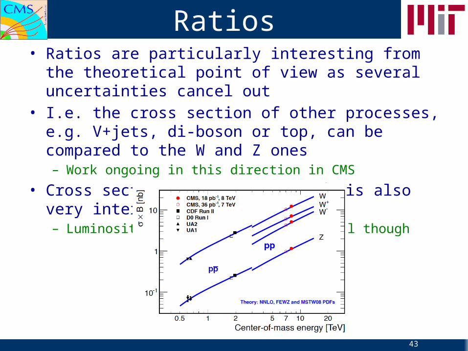
• Ratios are particularly interesting from the theoretical point of view as several uncertainties cancel out

• I.e. the cross section of other processes, e.g. V+jets, di-boson or top, can be compared to the W and Z ones– Work ongoing in this direction in CMS

• Cross section evolution with √s is also very interesting– Luminosity uncertainty doesn’t cancel though

Ratios

43

• An accurate measurement of the W and Z total and fiducial inclusive cross section at √s=8 TeV have been performed for the first time.– A dedicated dataset of low luminosity/pileup data has been used,

allowing a similar analysis as on 2010 data – Overall good agreement with theoretical predictions

• Luminosity measurement instrumental for this result– A lot of experienced gained during first LHC run especially for what

concerns luminosity absolute calibration (Van der Meer scan)– Error down to 2.6%, comparable with other experimental

uncertainties.

• Improvements to be expected for 13 TeV run

Conclusions

44

BACKUP

45

Factorizability

46

C. Barshel, LHCb beam gas analysis