M Number of fetuses showing ossification - sas.com · (TCPO). The study was set up as a 2x2...

The anticonvulsant phenytoin is known to be teratogenic on the prenatal development of inbred mice. Hartsfield et al. (1990) conducted a completely randomized experiment with 81 pregnant mice to investigate the possible synergistic effect of phenytoin (PHT) and trichloropropene oxide (TCPO). The study was set up as a 2x2 factorial; PHT and TCPO were the main factors. PHT was administered at the levels 0 mg/kg and 60 mg/kg, and TCPO was administered at 0 mg/kg and 100 mg/kg. The presence or absence of ossification in the phalanges on both the right and left forepaws on each of the fetuses is considered a measure of the teratogenic effect of the substances under study. In some phalanges the ossification did not occur at all; in some others, the ossification was almost complete. We selected the middle third phalanges because they yield around a 50% chance of ossification in the control groups. To simplify this part of our study further, we have analyzed only the response on the left middle third phalanx. Table 1.1 depicts the number of fetuses showing ossification in the middle third phalanx of the left forepaw out of the total number of fetuses in 11 mice that had been treated with both substances PHT and TCPO. This example is used here in a simple form to introduce the concept of overdispersion and will be revisited in greater depth in subsequent chapters.

1

Morel, Jorge, and Nagaraj Neerchal. Overdispersion Models in SAS®. Copyright © 2011, SAS Institute Inc., Cary, North Carolina, USA. ALL RIGHTS RESERVED. For additional SAS resources, visit support.sas.com/publishing.

http://support.sas.com/publishing

2 Overdispersion Models in SAS

Mouse j 1 2 3 4 5 6 7 8 9 10 11 Total

Number of fetuses showing ossification jt 2 0 1 7 0 0 0 0 6 1 1 18

Total number of fetuses jm 2 7 8 8 10 4 6 7 6 6 7 71

If jt and jm represent, respectively, the number of fetuses showing ossification and the total number of fetuses of the j-th mouse, j 1,2,...,11 , then the estimated probability of observing ossification in any middle third phalanx of the left forepaw can be calculated as

11

jj 1

11

jj 1

tˆ

m

which, in this example, turns out to be 18 0.253571

. If the jt 's were truly distributed as

Binomial random variables with parameters j,m , where is the underlying true probability

of ossification, an estimator of the variance of ̂ , given that mice are independent, would be

11

jj 1

ˆ ˆ1ˆ ˆVarm

The value of this estimated variance is 0.0027. Note that the above estimator is not valid if the Binomial model does not hold. Based on sampling theory (see Cochran 1977, p. 155), a consistent estimator, which does not depend on the binomial assumption, is

n2

j jj 1

2n

jj 1

ˆn (t m )ˆVar

m (n 1)

which turns out to be 0.0142. The remarkable difference between the model-based estimate and the sampling-theory estimate leads us to the following question: Are these data really binomially distributed with a common probability of success ? An easy way to answer this question is by computing the usual Pearson’s Chi-square


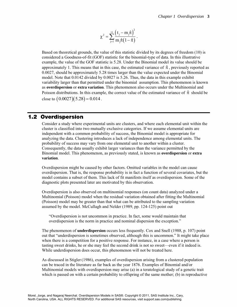
Chapter 1 Overdispersion 3

211

j j2

j 1 j

ˆt mˆ ˆm 1

.

Based on theoretical grounds, the value of this statistic divided by its degrees of freedom (10) is considered a Goodness-of-fit (GOF) statistic for the binomial-type of data. In this illustrative example, the value of the GOF statistic is 5.28. Under the Binomial model its value should be approximately 1. This means that in this case, the estimated variance of ̂ , previously reported as 0.0027, should be approximately 5.28 times larger than the value expected under the Binomial model. Note that 0.0142 divided by 0.0027 is 5.26. Thus, the data in this example exhibit variability larger than that permitted under the binomial assumption. This phenomenon is known as overdispersion or extra variation. This phenomenon also occurs under the Multinomial and Poisson distributions. In this example, the correct value of the estimated variance of ̂ should be close to 0.0027 5.28 0.014 .

Consider a study where experimental units are clusters, and where each elemental unit within the cluster is classified into two mutually exclusive categories. If we assume elemental units are independent with a common probability of success, the Binomial model is appropriate for analyzing the data. Clustering introduces a lack of independence among elemental units. The probability of success may vary from one elemental unit to another within a cluster. Consequently, the data usually exhibit larger variances than the variance permitted by the Binomial model. This phenomenon, as previously stated, is known as overdispersion or extra

variation.

Overdispersion might be caused by other factors. Omitted variables in the model can cause overdispersion. That is, the response probability is in fact a function of several covariates, but the model contains a subset of them. This lack of fit manifests itself as overdispersion. Some of the diagnostic plots presented later are motivated by this observation.

Overdispersion is also observed on multinomial responses (on count data) analyzed under a Multinomial (Poisson) model when the residual variation obtained after fitting the Multinomial (Poisson) model may be greater than that what can be attributed to the sampling variation assumed by the model. McCullagh and Nelder (1989, pp. 124-125) point out

“Overdispersion is not uncommon in practice. In fact, some would maintain that overdispersion is the norm in practice and nominal dispersion the exception.”

The phenomenon of underdispersion occurs less frequently. Cox and Snell (1988, p. 107) point out that “underdispersion is sometimes observed, although this is uncommon.” It might take place when there is a competition for a positive response. For instance, in a case where a person is tasting sweet drinks, he or she may feel the second drink is not so sweet—even if it indeed is. While underdispersion does occur, this phenomenon will not be treated here.

As discussed in Stigler (1986), examples of overdispersion arising from a clustered population can be traced in the literature as far back as the year 1876. Examples of Binomial and/or Multinomial models with overdispersion may arise (a) in a teratological study of a genetic trait which is passed on with a certain probability to offspring of the same mother; (b) in reproductive



toxicity experiments where chemicals are administered to litters and responses are measured on individual fetuses; (c) in experiments where individuals receiving treatments are allowed to interact with each other via support groups, as in stop-smoking programs or stop-drinking programs; (d) in household surveys where respondents within a household (or a neighborhood) may be strongly influenced by one or two individuals.

There are many papers that contain real examples which discuss and illustrate the overdispersion phenomenon and its consequences on erroneous inferences due to inflated Type I error rates. Some relevant examples in the areas of teratology and toxicology are given in Williams (1975, 1982), Williams et al. (1988), Kupper and Haseman (1978), Haseman and Kupper (1979), Kupper et al. (1986), Shirley and Hickling (1981), Paul (1982), Pack (1986), Lefkopoulou et al. (1989), Ryan (1992), Liang and McCullagh (1993), Carr and Portier (1993), Donner et al. (1994), Morel and Koehler (1995), and Morel and Neerchal (1997). Other important examples of overdispersion are found in Rosner (1984) and Donner (1989) in ophthalmology, Altham (1976) and Cohen

(1976) in studies of hospitalized sibling pairs, Crowder (1978) in the analysis of seed germination, Heckman and Willis (1977) in connection with a panel study, Efron (1986) in an epidemiology example involving toxoplasmosis in 34 cities of El Salvador, and Moore (1987) in the modeling of chromosome aberration in survivors of the atomic bomb of Hiroshima.

Early remarks regarding overdispersion under the Poisson model can be found in Student (1919). Examples of Poisson models with overdispersion can be found (a) in the analysis of counts and rates of longitudinal studies, and (b) in behavioral studies and in studies of number of accidents where there is inter-subject variability. Real examples of overdispersion under the Poisson model are found in the analysis of number of tumors in rats, Gail et al. (1980) and Lawless (1987); in a longitudinal clinical trial aimed to study the number of epileptic seizures, Breslow and Clayton (1993); and on the frequency of recurrence of bladder cancer, Dean and Balshaw (1997). An example with archaeological data is used by Efron (1992) to discuss the various patterns of overdispersion relative to Poisson variability; in another study, Zeger and Edelstein (1989) assess the efficacy of Vitamin C in reducing child mortality in Indonesia.

The phenomenon of binomial outcomes with overdispersion can be characterized in terms of the first two moments. Suppose that T is a Binomial random variable representing the number of successes out of m trials. Then,

E(T) = m , (1.1)

where represents the probability of success of each Bernoulli trial. Furthermore, if the Bernoulli trials m21 Y,...,Y,Y that encompass T satisfy the assumptions of the Binomial model, then Var(T) = m (1 ) . On the other hand, if they are positively correlated, then the usual assumption of independence in the Binomial model is violated. Let us denote the correlation between two Bernoulli trials by 2 2, 0 1 . We use 2 to indicate that the correlation is non-negative. Then, it can be shown that

2Var(T) = m (1 ){1+ (m 1)} . (1.2)



Note that while the expected value of T matches the Binomial model, its variance given in equation (1.2) is more than the variance modeled by a Binomial model because the factor

2{1+ (m 1)} is greater than one. A random variable T with mean and variance, as in equations (1.1) and (1.2), is said to have overdispersion or extra variation relative to the Binomial model. This simple structure of overdispersion has been well-recognized among sampling practitioners. See, for instance, equation 8.1 in Hansen et al. (1953), where the variance under one-stage cluster sampling is expressed as a function of the variance under simple random sampling. Similar observations can be found in the classical books on sampling by Kish (1965) and Cochran (1977). Among sampling practitioners, the parameter 2 represents the intra-cluster correlation and the

factor 2{1+ (m 1)} is the design effect. The case “positively correlated” corresponds to overdispersion. As previously stated, the occurrence of underdispersion is less common and corresponds to a negative correlation among the Bernoulli outcomes that comprise T.

Similarly, the definition of overdispersion can be extended to the case of Multinomial distribution. Consider a cluster consisting of m elemental units where the elemental units are being classified into (d+1) categories. Let T denote the d-dimensional vector of counts, corresponding to the first d categories, whose i-th component represents the number of elemental units classified into the i-th category. With clustered data, the vector T, which is usually modeled by a Multinomial distribution, often exhibit higher variability in the data than that allowed by the Multinomial model. In order to accommodate this overdispersion, the following moment structure is usually hypothesized as

E( ) = mT π (1.3) and

t 2Var( ) = m{Diag( ) - }{1+ ρ (m 1)}T π ππ , (1.4)

where t1 2 d( , ,..., ) π is a vector of probabilities, 10 i ,

d

ii 1

1

, and 2or

is the overdispersion parameter. If the multinomial-type variable T has mean vector and variance-covariance matrix as in equations (1.3) and (1.4), the variable T is said to have overdispersion relative to the Multinomial distribution. Note that when 0 the variance estimators in equations (1.2) and (1.4) reduce to that of the Binomial/Multinomial model. Several issues such as maximum likelihood estimation and Quasi-likelihood Models under the Multinomial distribution will be covered in Chapter 7.

Recall that for a Poisson random variable Y, E(Y) Var(Y) , 0 . Poisson random variable is a count of the number of occurrences of an event in a given time interval. As in the binomial case, there are underlying assumptions on the process for deriving the properties of a Poisson random variable. When these assumptions are not met, overdispersion may result. When Y is a Poisson-type of random variable, Y is said to have overdispersion if its first two moments are of the form

E(Y) , 0 (1.5)



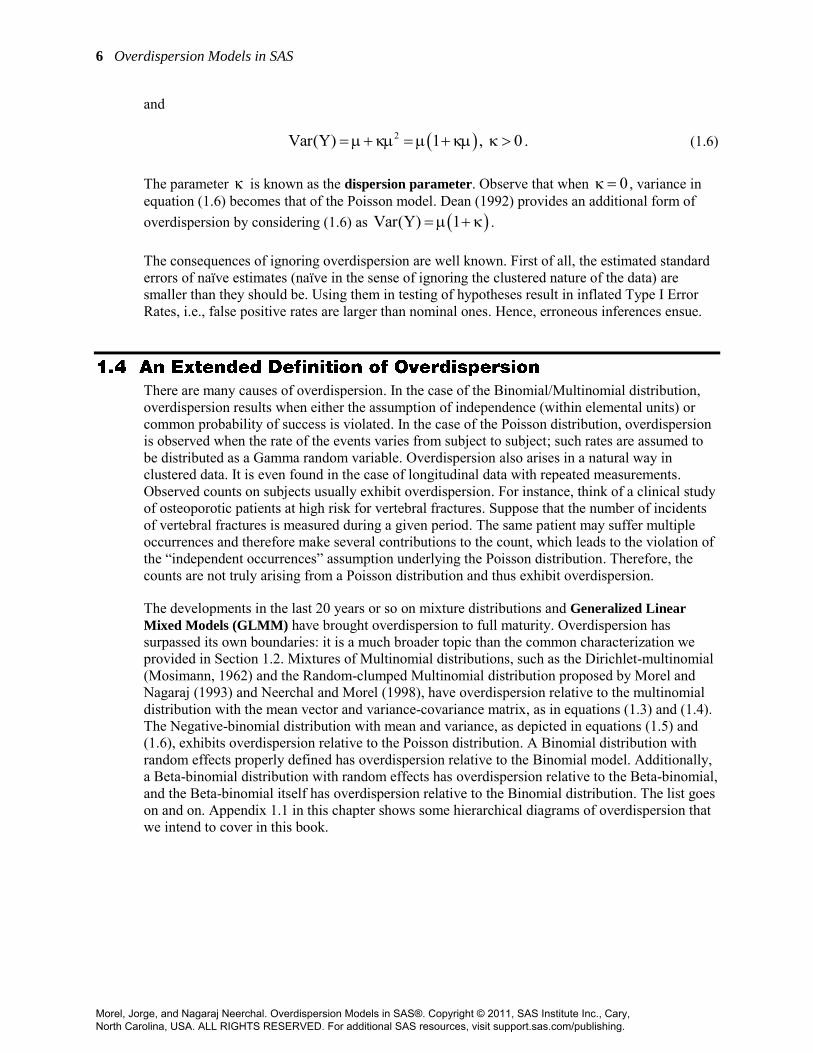
and

2Var(Y) 1 , 0 . (1.6)

The parameter is known as the dispersion parameter. Observe that when 0 , variance in equation (1.6) becomes that of the Poisson model. Dean (1992) provides an additional form of overdispersion by considering (1.6) as Var(Y) 1 .

The consequences of ignoring overdispersion are well known. First of all, the estimated standard errors of naïve estimates (naïve in the sense of ignoring the clustered nature of the data) are smaller than they should be. Using them in testing of hypotheses result in inflated Type I Error Rates, i.e., false positive rates are larger than nominal ones. Hence, erroneous inferences ensue.

There are many causes of overdispersion. In the case of the Binomial/Multinomial distribution, overdispersion results when either the assumption of independence (within elemental units) or common probability of success is violated. In the case of the Poisson distribution, overdispersion is observed when the rate of the events varies from subject to subject; such rates are assumed to be distributed as a Gamma random variable. Overdispersion also arises in a natural way in clustered data. It is even found in the case of longitudinal data with repeated measurements. Observed counts on subjects usually exhibit overdispersion. For instance, think of a clinical study of osteoporotic patients at high risk for vertebral fractures. Suppose that the number of incidents of vertebral fractures is measured during a given period. The same patient may suffer multiple occurrences and therefore make several contributions to the count, which leads to the violation of the “independent occurrences” assumption underlying the Poisson distribution. Therefore, the counts are not truly arising from a Poisson distribution and thus exhibit overdispersion.

The developments in the last 20 years or so on mixture distributions and Generalized Linear

Mixed Models (GLMM) have brought overdispersion to full maturity. Overdispersion has surpassed its own boundaries: it is a much broader topic than the common characterization we provided in Section 1.2. Mixtures of Multinomial distributions, such as the Dirichlet-multinomial (Mosimann, 1962) and the Random-clumped Multinomial distribution proposed by Morel and Nagaraj (1993) and Neerchal and Morel (1998), have overdispersion relative to the multinomial distribution with the mean vector and variance-covariance matrix, as in equations (1.3) and (1.4). The Negative-binomial distribution with mean and variance, as depicted in equations (1.5) and (1.6), exhibits overdispersion relative to the Poisson distribution. A Binomial distribution with random effects properly defined has overdispersion relative to the Binomial model. Additionally, a Beta-binomial distribution with random effects has overdispersion relative to the Beta-binomial, and the Beta-binomial itself has overdispersion relative to the Binomial distribution. The list goes on and on. Appendix 1.1 in this chapter shows some hierarchical diagrams of overdispersion that we intend to cover in this book.



A simple way of simulating correlated Bernoulli data is as follows. Let 0 01 mY,Y ,...,Y be

independent and identically distributed Bernoulli ( ) random variables. For each i, i=1,...,m, define iY as Y with probability , or as 0

iY with probability (1 ), 0 1 . In other words, each Yi can be represented by the mixture

0i i i iY Y I(U ) Y I(U ) , (1.7)

where the Ui are independent uniform (0,1) random variables, and I(.) denotes an indicator function. In this model for clumped data,

iE Y , iVar Y 1 and 21 2Corr Y ,Y .

The programming statements for generating data under model (1.7) are provided next for m=5,

0.6 and 2 0.3 . Note that n=20,000 clusters are being generated, each consisting of a string of m=5 correlated binary outcomes.

/*

Generation of correlated Bernoulli outcomes

For Y(1),Y(2),...,Y(m)

E(Y(i)) = Pi

Var(Y(i)) = Pi*(1-Pi)

Corr(Y(i),Y(i')) = Rho*Rho

*/

data correlated_bernoullis;

n = 20000; *--- Number of clusters;

m = 5; *--- Number of elemental units within the cluster;

pi = 0.6; *--- Probability of success of each elemental unit;

rho2 = 0.3; *--- Intra-cluster correlation;

seed = 16670;

rho = sqrt( rho2 );

do subjid = 1 to n;

yy = 0; *--- Variable yy plays the role of y of eq. (1.7);

u = uniform( seed );

if u < pi then yy = 1;

do i=1 to m;

y = 0;

u = uniform( seed );

if u < rho then y = yy;

else do;

uu = uniform( seed );

if uu < pi then y = 1;

end;

output;

end;

end;

keep subjid i y;

run;



proc transpose data=correlated_bernoullis out=new;

by subjid;

id i;

var y;

run;

ods html;

proc corr data=new;

var _1 - _5;

run;

ods html close;

proc transpose data=correlated_bernoullis out=new;

by subjid;

id i;

var y;

run;

ods html;

proc corr data=new;

var _1 - _5;

run;

ods html close;

Output 1.1 indicates that the means of each iY is (as expected) approximately 0.6 . The

estimated standard deviations are about 1 0.6 0.4 0.4849 . The estimated

correlations among elemental units are about 2 0.3 . Note that the correlation structure of the

repeated measurements is exchangeable. That is, 2i tCorr Y ,Y , i t, for i, t 1,2,...,m.

The CORR Procedure

5 Variables: _1 _2 _3 _4 _5

Simple Statistics

Variable N Mean Std Dev Sum Minimum Maximum

_1 20000 0.59995 0.48992 11999 0 1.00000

_2 20000 0.60305 0.48928 12061 0 1.00000

_3 20000 0.59855 0.49020 11971 0 1.00000

_4 20000 0.60065 0.48978 12013 0 1.00000

_5 20000 0.60140 0.48962 12028 0 1.00000



Pearson Correlation Coefficients, N = 20000

Prob > |r| under H0: Rho=0

_1 _2 _3 _4 _5

_1 1.00000

0.29579

<.0001

0.31689

<.0001

0.30128

<.0001

0.29763

<.0001

_2 0.29579

<.0001

1.00000

0.28872

<.0001

0.29704

<.0001

0.27709

<.0001

_3 0.31689

<.0001

0.28872

<.0001

1.00000

0.32044

<.0001

0.30346

<.0001

_4 0.30128

<.0001

0.29704

<.0001

0.32044

<.0001

1.00000

0.29617

<.0001

_5 0.29763

<.0001

0.27709

<.0001

0.30346

<.0001

0.29617

<.0001

1.00000

If we let m

ii 1

T Y

, iY 's defined as in equation (1.7), it can be shown E(T) = m and

2Var(T) = m (1 ){1+ (m 1)} . Therefore, the binomial-type random variable T derived from the mixture model (1.7) exhibits overdispersion relative to the Binomial distribution. Thus, for m=5, 0.6 and 2 0.3 , the target values for the mean and the variance in the simulation

are E T m 5 0.6 3.00 and

2Var(T) = m (1 ){1+ (m 1)}= 5 0.6 0.4 2.2 2.64 , which can be verified by adding the following statements to Program 1.1. We obtain 3.004 and 2.636 as empirical estimates of the mean and variance, respectively, in our simulation using 20,000 replications.

*--- Program 1.1 Continued;

proc means data=correlated_bernoullis sum noprint;

class subjid;

var y;

output out=out1 sum=t;

run;

data out1;

set out1;

if _type_ = 1;

drop _type _freq_;

run;



ods html;

proc means data=out1 mean var maxdec=2;

var t;

run;

ods html close;

Recall that one of the consequences of overdispersion in the data is inflated Type I Errors. Program 1.1 can be easily extended to a simulation to demonstrate this undesirable effect. To this end, consider a sample of n=20 clusters each of size m=5. If the elemental units within the clusters are treated as independent, then we will have a total of 100 Bernoulli trials with the same probability of success . We need to test the null 0H : 0.6 versus the alternative hypothesis

1H : 0.6 . For the Binomial distribution, the Z-test at 0.05 is to reject the null when

ˆ 0.6Z 1.6449ˆ ˆ1 /100

. An estimate of the true Type I Error can be obtained by

performing this test on a series of overdispersed data sets generated by Program 1.1, and then by computing the percentage of rejections. Program 1.2 provides the necessary statements to perform this simulation.

*--- Estimating actual Type I Error rate for overdispersed data;

data correlated_bernoullis; *--- This data set was created in Program 1.1;

set correlated_bernoullis;

reps = ceil( subjid / 20 ); *--- Creates 1000 reps of n=20 clusters of size m=5 each;

run;

proc means data=correlated_bernoullis mean noprint;

class reps;

var y;

output out=test mean=Pi_hat;

run;

data test;

set test;

if _type_ = 1;

z = (Pi_hat - 0.6) / sqrt( Pi_hat*(1-Pi_hat) / 100 );

P_val = 0;

if z > 1.6449 then P_val = 1;

run;

title "Monte Carlo Estimate of Type I Error Rate";

proc means data=test n mean maxdec=3;

var P_val;

run;

For 2 0.3 , the estimated Type I Error rate turns out to be 0.160, about three times the nominal level of 0.05. We can now rerun Programs 1.1 and Program 1.2, appropriately concatenated for other values of 2 . The following table provides a summary for three runs using the same seed as above for convenience.



α = 0.05

2 (Overdispersion) Actual Type I Error Rate 0.3 0.160 0.5 0.197 0.7 0.210

We hope that this simple example has convinced the reader that study of overdispersion is very important from the point of view of making accurate statistical inferences in practical situations. Many methods of taking overdispersion into account in several commonly used models are discussed in this book.

Several of the main topics to be covered in this book, namely Quasi-likelihood Functions, Generalized Linear Models (GLM), Generalized Estimating Equations (GEE), and Generalized Linear Mixed Models (GLMM), are motivated by the generality of the many statistical methods applicable to all members of the exponential family. Therefore, we begin with a brief introduction to the exponential family of densities by outlining some of their basic properties. The exponential family is a class of density functions sharing certain characteristics and properties. Among the members of this family are the Normal, Bernoulli, Binomial, Multinomial, Poisson, Negative-binomial, Beta, and Gamma distributions. This family of distributions plays a very important role in the classical statistical inference topics. Following the literature, we use the canonical parameter and canonical link function set up for our discussion, but all examples will be in the familiar notation, which may be or not be canonical.

A density function in this family can be written as

y b

f y exp c y,f

, (1.8)

where b . and c . are some specific functions. The parameter is a real-valued location

parameter and is known as the natural (or canonical) parameter. The function b is referred to as the cumulant and the parameter as the dispersion (or scale) parameter. We assume that

b is continuously twice differentiable. In the case of the Normal distribution, the parameter

corresponds to the variance 2 and is functionally unrelated with the mean. On the other



hand, in other distributions such as Bernoulli, Binomial, and Poisson, mean and variance are given by a single parameter and consequently, in the likelihood function (1.8) the dispersion parameter is not present in the sense that 1 . Therefore, an additional parameter, 1 , is included to accommodate data with overdispersion. More information about this issue will follow in the next chapter.

If Y is a random variable whose density function belongs to the exponential family, then it can be shown that the mean and variance of Y are related to the cumulant function as follows

b

E(Y)

(1.9)

and

2

2

bVar(Y)

, (1.10)

where b

and

2

2

b

denote the first and second derivatives of the function b with

respect to .

Note that in equation (1.9) the parameter is expressed as a function of . This relationship is known as the canonical link function or as the natural link function. We will denote the canonical link function as g . Obviously, 1g since b . is an invertible function

with smooth first and second derivatives. The function 1g . , which is nothing but the first

derivative of the function b . , is known as the mean function. It seems as if we were going around in circles; however, it is important to distinguish between the link and the mean functions.

The variance of Y is the product of two terms, the dispersion parameter and the second

derivative of b . The latter is known as the variance function and depends on the mean

through the first derivative of b . Thus, the variance function is a function of and will be

denoted by v . Hence, equation (1.10) can be written as

Var(Y) v . (1.11)



Table 1.3 shows the main features of the Bernoulli and Poisson distributions as members of the exponential family. Note that for the Bernoulli distribution, the mean and canonical link functions are the logistic and logit functions. They are also the same for the Binomial distribution (not depicted in Table 1.3). For the Poisson, the exponential and logarithmic functions are, respectively, the associated mean and link functions.

Distribution

Feature Bernoulli Poisson

Probability function (usual form)

1 yy 1 , y 0,1, 0 1 ye , y 0,1,2,..., 0

y!

Cumulant b log 1 e exp

Mean function e1 e

(logistic function)

exp (exponential function)

Canonical link function log

1

(logit link) log (logarithm link)

Dispersion parameter 1 1

Variance function v 1

Probability function (canonical form) exp yln ln 1

1

exp yln ln y!



Binomial Distribution

Beta-binomial

1) Binomial Distribution

Beta-binomial

with Random Effects

Binomial Marginal Models

GEE Type

Random-clumped Binomial

Zero-inflated Binomial

Random-clumped Binomial

with Random Effects

Binomial with Random Effects, Conditional Models, GLMM Type

Poisson Distribution

Negative-binomial

Poisson Marginal Models

GEE Type

Zero-inflated Negative-binomial

Zero-inflated Poisson

Zero-inflated Negative-binomial

with Random Effects

Poisson Distribution with Random Effects

Conditional Models, GLMM Type

Hurdle Models

Zero-inflated Poisson

with Random Effects

2) Poisson Distribution

Appendix 1.1: Hierarchical Models to be Covered in this Book

Appendix 1.1 (Cont.): Hierarchical Models to be Covered in this Book

Multinomial Distribution

Multinomial Marginal Models GEE Type

3) Multinomial Distribution

Multinomial with Random Effects, Conditional Models, GLMM Type

Dirichlet-multinomial

Random-clumped Multinomial


M Number of fetuses showing ossification - sas.com · (TCPO). The study was set up as a 2x2...

Documents

Transcript of M Number of fetuses showing ossification - sas.com · (TCPO). The study was set up as a 2x2...