M. Montalto - Centro de Astrofísica · Introduction to photometry M. Montalto ... standard...
49
Introduction to photometry M. Montalto Centro de Astrofísica da Universidade do Porto (CAUP), Advanced Course May 22- Jun 5 2014
Transcript of M. Montalto - Centro de Astrofísica · Introduction to photometry M. Montalto ... standard...

Introduction to photometry
M. Montalto
Centro de Astrofísica da Universidade do Porto (CAUP), Advanced Course May 22- Jun 5 2014

Introduction to photometry
First theoretical lesson 22 May 2014 13:30 Auditorium
First practical lesson 23 May 2014 13:30 Classroom
Second theoretical lesson 29 May 2014 13:30 Auditorium
Second practical lesson 30 May 2014 13:30 Classroom
Third practical lesson 5 June 2014 13:30 Classroom
Centro de Astrofísica da Universidade do Porto (CAUP), Advanced Course May 22- Jun 5 2014

The Human eye
Advanced Course on photometry May 22- Jun 5 2014
In the human eye there are two kinds of photoreceptors: the rods and the cones.

The Almagest
Advanced Course on photometry May 22- Jun 5 2014
The Almagest is a 2nd-century mathematical and astronomical treatise written by Claudius Ptolemy.
Books VII and VIII cover the motions of the fixed stars, including precession of the equinoxes and documents the work of Hipparchus presenting a star catalogue of 1022 stars, described by their positions in the constellations and their brightness.
The error on the brightness estimate was around 0.5 mag.

Abd al-Rahman al-Sufi (903 - 986)
Advanced Course on photometry May 22- Jun 5 2014
He wrote the "Book of Fixed Stars" where he revised the Hipparchus work providing its own measurements of stellar brightnesses and positions.
He improved the accuracy of the magnitudes estimates at the level of 1/3rd of a magnitude.

Magnitudes
Advanced Course on photometry May 22- Jun 5 2014
The modern definition of magnitudes was introduced by Pogson (1856):
Color:
Color excess:
Reddening:
A shift in color toward larger values due to an increased absorption at bluer wavelengths (e. g. interstellar reddening, atmospheric reddening)
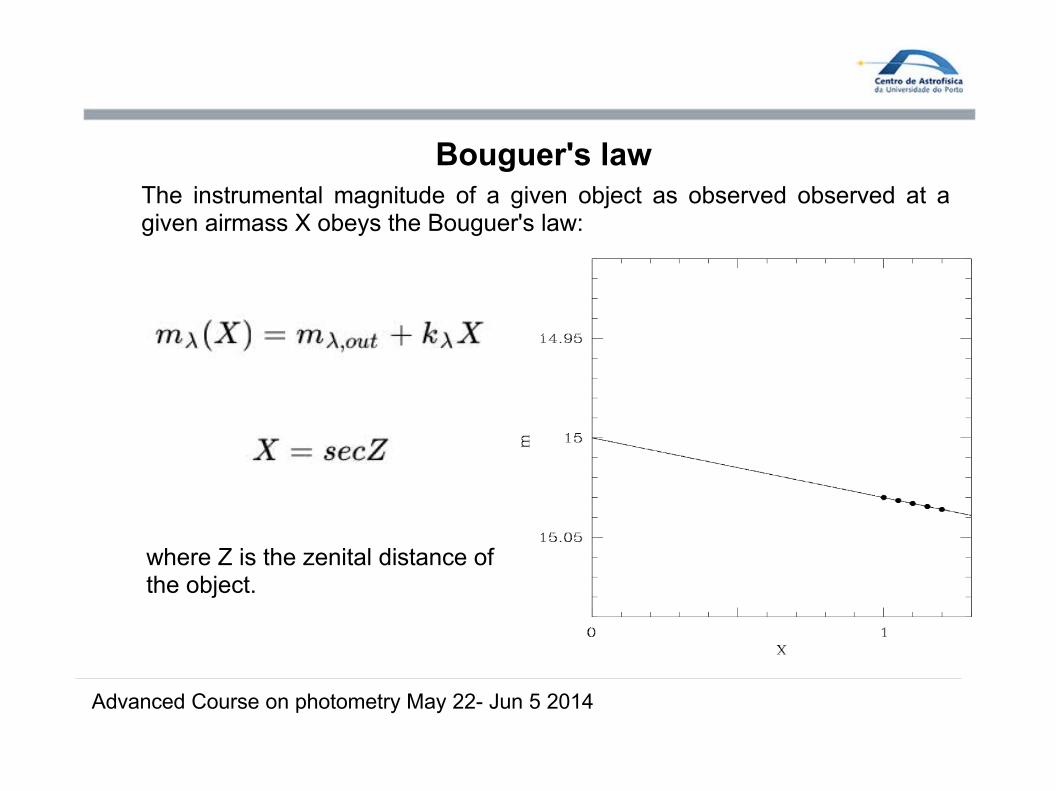
Bouguer's law
Advanced Course on photometry May 22- Jun 5 2014
The instrumental magnitude of a given object as observed observed at a given airmass X obeys the Bouguer's law:
where Z is the zenital distance of the object.

Photographic photometry
Advanced Course on photometry May 22- Jun 5 2014
Photographic photometry was introduced in the XIXth century
The kind of emulsions used at the beginning were more sensitive to the blue than the eye, p_g
Later on panchromatic emulsions were introduced resulting in the photo-visual magnitudes, p_v
Non-linear processes convert light into dark grains in the emulsion
The skilled group of observers of the Harvard College Observatory led by E. Pickering was able to achieve an accuracy of 1/6th magnitudes against 1/10th magnitudes achieved by photographic plates

Photographic photometry
Advanced Course on photometry May 22- Jun 5 2014
Iris type photometer

The North Polar Sequence
Advanced Course on photometry May 22- Jun 5 2014
The introduction of this novel instrument required the establishment of a photographic magnitude scale to be linked with the visual scale.
It was decided that a group of stars (originally consisting of 47 members) around the North Pole, selected by E. Pickering as part of the Harvard Observing programme should have defined the basic photographic (pg) magnitude scale.
The mean of all p_g magnitudes for the North Polar Sequence stars of spectral type A0 in the magnitude range between 5.5-6.5 was equal to the mean of the visual magnitudes for those same stars as determined by the Harward meridian photometry.

Photomultipliers
Advanced Course on photometry May 22- Jun 5 2014
Photomultipliers were introduced at the beginnng of th XXth century
They are based on the photoelectric effect and on the secondary emission effect
The most famous of them for astronomical applications is the 1P21 photomultiplier developed by RCA
Spectral response between 300 and 650 nm
Quantum efficiency around 10%
DeWitt & Seyfert 1950, PASP, 62, 369 estimates 0.005 mag error on mag 7 star using a 30 cm telescope

UBV Johnson & Morgan system
Advanced Course on photometry May 22- Jun 5 2014
(Johnson & Morgan 1953, 117, 313)
1) It was defined by Johnson & Morgan in the early 1950s and it is the most widespread used broadband photometric system.
2) The V magnitude is in agreement with photovisual magnitudes and the zero point of the B-V and U-B color scale is set by the average color of A0V stars.
3) It was defined using the 1P21 photomultiplier
4) It employed three broadband colored glass filters
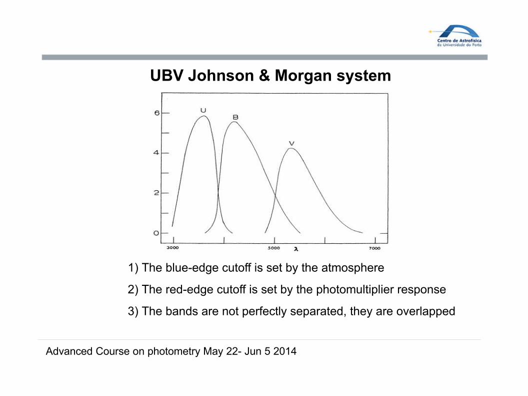
UBV Johnson & Morgan system
Advanced Course on photometry May 22- Jun 5 2014
1) The blue-edge cutoff is set by the atmosphere
2) The red-edge cutoff is set by the photomultiplier response
3) The bands are not perfectly separated, they are overlapped

UBV Johnson & Morgan system
Advanced Course on photometry May 22- Jun 5 2014
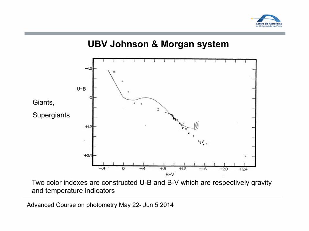
Two color indexes are constructed U-B and B-V which are respectively gravity and temperature indicators
Dwarfs
UBV Johnson & Morgan system
Advanced Course on photometry May 22- Jun 5 2014
Two color indexes are constructed U-B and B-V which are respectively gravity and temperature indicators
Giants,
Supergiants

UBV Johnson & Morgan system
Advanced Course on photometry May 22- Jun 5 2014
The Q-index – a reddening free index
For early type stars (B1-B9) knowing the luminosity class it is possible to construct a reddening free index:

TCMDs and CMDs
Advanced Course on photometry May 22- Jun 5 2014
NGC2158, Carraro G., Girardi L., Marigo P. 2002, MNRAS, 332, 705

Photometric systems
Advanced Course on photometry May 22- Jun 5 2014
Photometric systems like the Johnson system allow us to place the measurements into a standard flux scale
=> Remove the effect of the atmospheric absorption
=> Calibrate the sensitivity of the instrument
This calibration is achieved by observing networks of constant brightness stars, called standard stars, which define the photometric system through their magnitudes and colors measured at specific bandpasses with a specific instrument

Photometric systems
Advanced Course on photometry May 22- Jun 5 2014
The relationship between the observer instrumental system and the standard system is usually of the form:
There are more than 200 photometric systems (The Asiago Database of photometric systems, http://ulisse.pd.astro.it/Astro/ADPS/)

Observational complications with standard photometry
Advanced Course on photometry May 22- Jun 5 2014
Observers set-up
A) Observers' filters may not correspond to that one of the standard system, and the present instrumentation may not match the original one
B) Not observing standards with a sufficiently large color baseline to encompass all the objects of interest
C) In large field of view cameras off-axis effects on intereference filters cause the bandwith of the filter to change across the field of view.
D) Slow shutters can introduce variations in intensity across the field
Observational complications with standard photometry
Advanced Course on photometry May 22- Jun 5 2014
Standard lists
A) Standard stars often do not represent all kind of stars
B) Standard lists may contain group of stars systematically different from a truly representative sample because of their position in the Galaxy
=> Standards should be selected in a wide range of RAs, DECs and magnitudes

Observational complications with standard photometry
Advanced Course on photometry May 22- Jun 5 2014
Aperture or diafragm sizes
Photoelectric photometry requires large apertures. Landolt standards require apertures between 14-27 arcsec
=> Aperture corrections need to be applied in crowded fields or networks of secondary standards should be used (Stetson et al. 2000, PASP, 112, 925)
Summary
Advanced Course on photometry May 22- Jun 5 2014
We have briefly reviewed the crucial steps concerning the historical development of the photometric technique from the time of visual observations to that one of photomultipliers
We have introduced the definitions of magnitude, color, color excess and reddening
We have discussed the atmospheric extinction effect and the Bouguer's law
We have introduced the UBV Johnson & Morgan system discussing its strenght and limitations
We have seen the importance that the construction of photometric systems had to prompt our understanding of the physical properties of stars
We have discussed the limitations inherent in the process of performing standard photometry and the factors that limit its accuracy

Introduction to photometry
M. Montalto
Centro de Astrofísica da Universidade do Porto (CAUP), Advanced Course May 22- Jun 5 2014

Introduction to photometry
M. Montalto
Centro de Astrofísica da Universidade do Porto (CAUP), Advanced Course May 22- Jun 5 2014

Introduction to photometry
First theoretical lesson May 22, 2014 13:30 Auditorium
First practical lesson May 23, 2014 13:30 Classroom
Second theoretical lesson May 29, 2014 13:30 Auditorium
Second practical lesson May 30, 2014 13:30 Classroom
Third practical lesson June 5, 2014 13:30 Classroom
Centro de Astrofísica da Universidade do Porto (CAUP), Advanced Course May 22- Jun 5 2014

In the last lesson...
Advanced Course on photometry May 22- Jun 5 2014
1) Historical overview
2) Definitions of magnitude, color, color excess and reddening
3) Atmospheric extinction effect and the Bouguer's law
4) UBV Johnson & Morgan system, color-color, color-magnitude diagrams
5) Photometric systems
6) Limitations inherent in the process of performing standard photometry
Standard vs. differential photometry
Advanced Course on photometry May 22- Jun 5 2014
Standard photometry
Standard (or absolute) photometry refers to photometric measurements reported in a standard photometric system by means of a calibration process. This procedure permits to obtain the absolute flux of a given source.
=> spectral type, gravity, reddening, age, distance
Differential photometry
Differential photometry refers to photometric measurements of a given source with respect to one or more comparison sources which absolute flux is not necessarily known.
=> relative flux variations, lightcurves
CCDs
Advanced Course on photometry May 22- Jun 5 2014
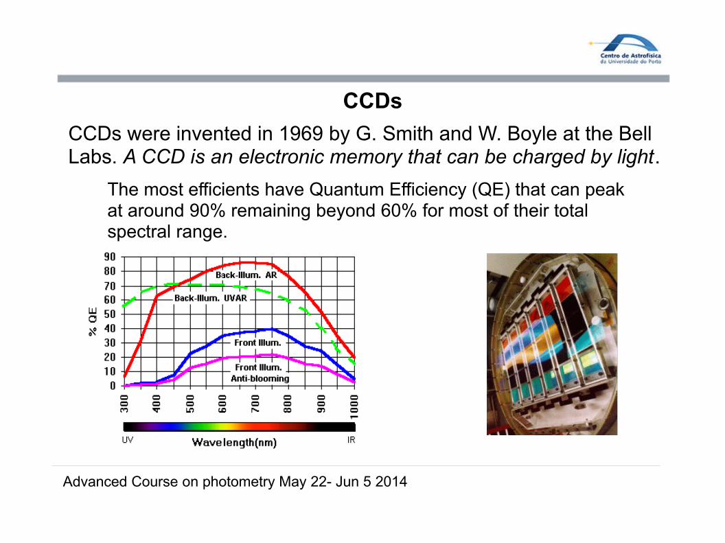
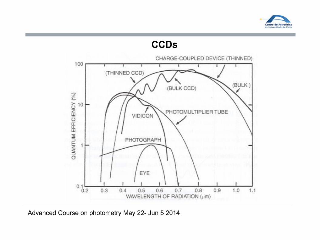
CCDs were invented in 1969 by G. Smith and W. Boyle at the BellLabs. A CCD is an electronic memory that can be charged by light.
The most efficients have Quantum Efficiency (QE) that can peak at around 90% remaining beyond 60% for most of their total spectral range.
CCDs
Advanced Course on photometry May 22- Jun 5 2014

CCDs: functioning
Advanced Course on photometry May 22- Jun 5 2014
(Janesick & Blouke 1987, Sky and Telescope Magazine, September, 74, 238)
Photons hit the silicon within a pixeland are absorbed.
Silicon releases a valence electron inthe conduction band.
The freed electrons are hold within apotential well within each pixel.
Each raw is shifted in the output output register register and each pixel in the output register is shifted out in the output output electronics.electronics.
The output voltage from a given pixel Is converted to a digital number by an A/D converter (ADUs=analog-to-digital units)
GAIN GAIN = the number of required electrons to produce 1 ADU (-e/ADU)

CCDs: basics
Advanced Course on photometry May 22- Jun 5 2014
Readout noiseReadout noise: the number of electrons that is introduced per pixel upon readout of the device (5 e/pix). - conversion from analog signal to digital signal - electronics introduces spurious electrons
Readout timeReadout time: time required to readout the entire array of pixels
Full Well Capacity: the amount of charge a pixel can hold in normal operations (85000-350000 electrons)
Binning: binning permits to coadd the charge of adjacent pixels into one superpixel, before A/D conversion, and then read out the entire pixel
Windowing: windowing permits to select a sub-region of the detector to be read-out upon completion of the integration

Overview of the reduction process
Advanced Course on photometry May 22- Jun 5 2014
Bias/Dark Flat-fieldScience Calibratedimages
Calibration
PSFApertureImageSubtractionAnalysis
Detrending
Pre-reduction
Reduction
Post-reduction

Bias
Advanced Course on photometry May 22- Jun 5 2014
CCDs are set-up in order to provide a positive offset value foreach image. To measure this value two approaches are used:
Nordic Optical Telescope (NOT) ALFOSC bias
Bias images are zero exposuretime images taken with the shutter closed.
Overscan strips are rows or columns both added and stored with each image frame.
Bias level can vary (smoothly)with time.
Bias images Master Bias

Dark images
Advanced Course on photometry May 22- Jun 5 2014
CCDs thermal noise produces spurious electrons which are accumulated together with scientific electrons. Thermal noise is a strong function of temperature and is given in -e/px/hr.
To mitigate this effect CCDs are cooled down usually with liquid nitrogen.
Dark images Master Dark
The master dark is then subtracted from all the images

Flat fielding
Advanced Course on photometry May 22- Jun 5 2014
Flat fields are constant illumination images acquired to flat the relative response of each pixel to the incoming radiation.
Flat fields can be acquired usingpredisposed screens illuminatedby lamps in the telescope building=> Dome flats
Observing the sky during twilight=> Sky flats
Ideally all pixels should be uniformly illuminatedat each wavelength, with a source having the same spectrum of the target object
Flat images
For each filter:
Master Flat, FF
Normalized Master Flat, FFNN

Flat fielding
Advanced Course on photometry May 22- Jun 5 2014
Isaac Newton Telescope (INT), WFI, CCD-1R-band flat-field
Himalayan Chandra TelescopeR-band flat
Fringing
Advanced Course on photometry May 22- Jun 5 2014
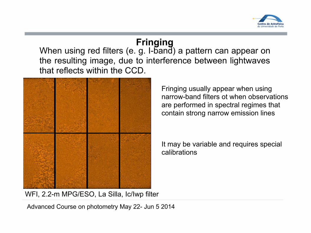
When using red filters (e. g. I-band) a pattern can appear on the resulting image, due to interference between lightwaves that reflects within the CCD.
WFI, 2.2-m MPG/ESO, La Silla, Ic/Iwp filter
Fringing usually appear when usingnarrow-band filters ot when observationsare performed in spectral regimes thatcontain strong narrow emission lines
It may be variable and requires specialcalibrations

Science calibrated images
Advanced Course on photometry May 22- Jun 5 2014
A science calibrated image is obtained subtracting for each pixelthe masterbias and dividing by the normalized masterflat.

S/N calculation
Advanced Course on photometry May 22- Jun 5 2014
The Signal to Noise of a given pixel or of a group of pixels is given by:
N* is the total number of photons from the source
NS is the total number of photons/pix from the background
ND is the total number of dark current electrons/pix
RON is the read out noise (in electrons)
Aperture photometry
Advanced Course on photometry May 22- Jun 5 2014
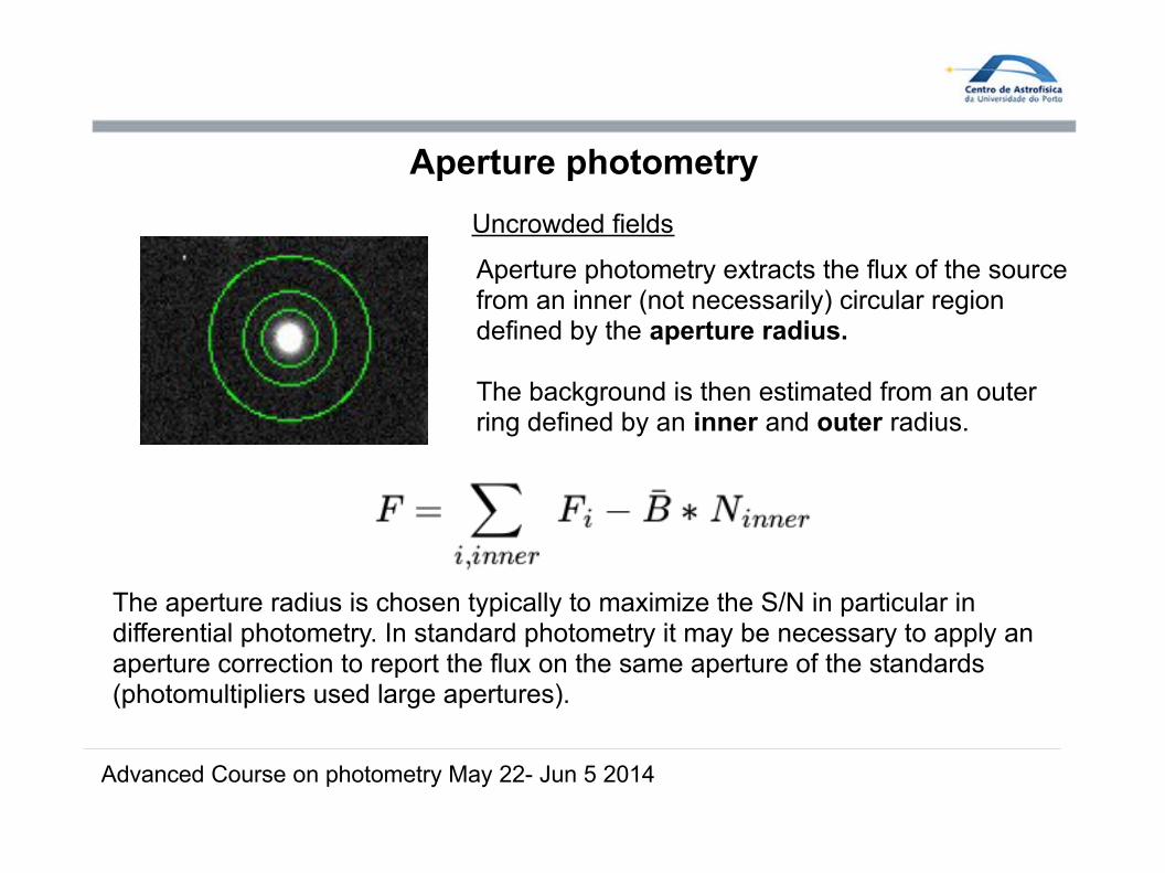
Uncrowded fields
Aperture photometry extracts the flux of the sourcefrom an inner (not necessarily) circular region defined by the aperture radius.
The background is then estimated from an outerring defined by an inner and outer radius.
The aperture radius is chosen typically to maximize the S/N in particular in differential photometry. In standard photometry it may be necessary to apply anaperture correction to report the flux on the same aperture of the standards(photomultipliers used large apertures).

PSF: point spread function
Advanced Course on photometry May 22- Jun 5 2014
In absence of atmosphere and for a perfect circular lens the image of a focusedstar would be diffraction limited and given by the Airy disk:
At 550 nm for a 8m telescope this gives 0.014 arcsec. From the ground under the best conditions it is possible to achieve around 0.3 arcsec.
Atmospheric turbulent mixing blurrs the final image. Moreover optical aberrations,distortions, telescope tracking problems may all affect the final shape of the PSF.
PSF: point spread function
Advanced Course on photometry May 22- Jun 5 2014
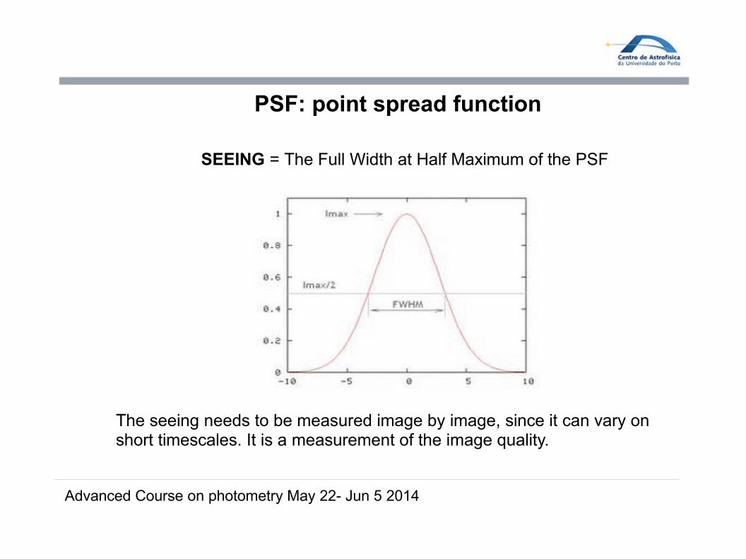
SEEING = The Full Width at Half Maximum of the PSF
The seeing needs to be measured image by image, since it can vary onshort timescales. It is a measurement of the image quality.

PSF photometry
Advanced Course on photometry May 22- Jun 5 2014
Crowded fields
PSF photometry models the PSF function by means of different approaches:
1) A purely empirical PSF is assumed by stacking together the brightest and most isolated sources;
2) A purely analytical PSF is constructed by means of a non-linear least square fit of the stacked averaged brightest and isolated sources;
3) A semi-empirical PSF is constructed by fitting an analytic function within a core radius (fitting radius), and a look-up table of the residuals is constructed by stacking the residuals of the brightest sources.
The model is then fit to the data scaling and shifting the PSF to the position of eachdifferent source that has been previously cataloged.

Image subtraction photometry
Advanced Course on photometry May 22- Jun 5 2014
Image subtraction is used essentially in differential photometry.
1) A stacked reference image is created from the best seeing images.
2) All the images are registered to the reference astrometric system
3) The reference is subtracted from the images leaving only residual images.
(Alard & Lupton 1998; Alard 2000)

Lightcurve creation
Advanced Course on photometry May 22- Jun 5 2014
Lightcurves are created selecting a sample of comparison stars on thesame field of the target(s).
These stars should be ideally close to the objects we want to measure,both spatially and also in color.
A superstar is formed summing up the flux of the comparisons and therebyThe flux of the target is divided by the comparisons.

Detrending
Advanced Course on photometry May 22- Jun 5 2014
Photometric time series might present systematic variations due to several effects.
-Observational conditions are changing during the night(seeing, clouds, background variations...)
-Instrumental effects like inaccurate pointing, change of temperature of the detector
-Inaccurate reduction of the data, badly determined PSFs, bad reference frames, wrong apertures

Detrending
Advanced Course on photometry May 22- Jun 5 2014
Two approaches are generally applied to correct for these systematics:
External Parameter Decorrelation EPD Magnitudes are decorrelated against a given set of external parameters, such like airmass, seeing, centroid positions. This leads in general to linear least square equations.
Trend Filtering Algorithm TFA We consider some template lightcurves and search for the best linear combination of these lightcurves which is Then subtracted from the signal.
SysRem Tamuz, Mazeh & Zucker (2005, MNRAS, 356, 1466)

Summary
Advanced Course on photometry May 22- Jun 5 2014
We defined the difference between standard and differential photometry
We discussed CCDs properties and characteristics
We presented the major steps in data reduction analysis, subdividing this process in pre-reduction, reduction and post-reduction
We considered three major photometric techniques:Aperture photometry, PSF photometry and Image subtraction
We discussed lightcurve creation and introduced lightcurve detrending algorithm