M -MIG: INFORMATION THEORETIC APPROACH FOR J L CROWDS

Published as a conference paper at ICLR 2019

MAX-MIG: AN INFORMATION THEORETIC APPROACHFOR JOINT LEARNING FROM CROWDS

Peng Cao∗, Yilun Xu∗School of Electronics Engineering and Computer Science,Peking University{caopeng2016,xuyilun}@pku.edu.cn

Yuqing KongThe Center on Frontiers of Computing Studies,Peking [email protected]

Yizhou WangNat’l Eng. Lab. for Video TechnologyComputer Science Dept., Peking UniversityCooperative Medianet Innovation CenterPengCheng LabDeepwise AI [email protected]

ABSTRACT

Eliciting labels from crowds is a potential way to obtain large labeled data. De-spite a variety of methods developed for learning from crowds, a key challengeremains unsolved: learning from crowds without knowing the information structureamong the crowds a priori, when some people of the crowds make highly correlatedmistakes and some of them label effortlessly (e.g. randomly). We propose aninformation theoretic approach, Max-MIG, for joint learning from crowds, witha common assumption: the crowdsourced labels and the data are independentconditioning on the ground truth. Max-MIG simultaneously aggregates the crowd-sourced labels and learns an accurate data classifier. Furthermore, we devise anaccurate data-crowds forecaster that employs both the data and the crowdsourcedlabels to forecast the ground truth. To the best of our knowledge, this is the firstalgorithm that solves the aforementioned challenge of learning from crowds. Inaddition to the theoretical validation, we also empirically show that our algorithmachieves the new state-of-the-art results in most settings, including the real-worlddata, and is the first algorithm that is robust to various information structures.

1 INTRODUCTION

Lack of large labeled data is a notorious bottleneck of the data-driven-based machine learningparadigm. Crowdsourcing provides a potential solution to this challenge: eliciting labels from crowds.However, the elicited labels are usually very noisy, especially for some difficult tasks (e.g. ageestimation, medical images annotation). In the crowdsourcing-learning scenario, two problems areraised:

(i) how to aggregate and infer the ground truth from the imperfect crowdsourced labels?

(ii) how to learn an accurate data classifier with the imperfect crowdsourced labels?

One conventional solution to the two problems is aggregating the crowdsourced labels using majorityvote and then learning a data classifier with the majority answer. However, this naive method willcause biased results when the task is difficult and the majority of the crowds label randomly or alwayslabel a particular class (say class 1) effortlessly.

Another typical solution is aggregating the crowdsourced labels in a more clever way, like spectralmethod (Dalvi et al., 2013; Zhang et al., 2014), and then learning with the aggregated results. Thismethod avoids the above flaw that the majority vote method has, as long as their randomnesses are∗Equal Contribution.

1


mutually independent. However, the spectral method requires that the experts’ labeling noise aremutually independent, which often does not hold in practice since some experts may make highlycorrelated mistakes (see Figure 2 for example). Moreover, the above solutions aim to train an accuratedata classifier and do not provide a method that can employ both the data and the crowdsourced labelsto forecast the ground truth.

A common assumption in the learning from crowds literature is that conditioning on the groundtruth, the crowdsourced labels and the data are independent, as shown in Figure 1 (a). Under thisassumption, the crowdsourced labels correlate with the data due to and only due to the groundtruth. Thus, this assumption tells us the ground truth is the “information intersection” between thecrowdsourced labels and the data. This “information intersection” assumption does not restrict theinformation structure among the crowds i.e. this assumption still holds even if some people of thecrowds make highly correlated mistakes.

Figure 1: (a) The general information structure under the “information intersection” assumption.(b) Possible information structures under the “information intersection” assumption, where thecrowdsourced labels are provided by several experts: (1) independent mistakes: all of the experts arecorrelated with the ground truth and mutually independent of each other conditioning on the groundtruth; for (2), (3) the senior experts are mutually conditional independent and (2) naive majority: thejunior experts always label class 1 without any effort; (3) correlated mistakes: the junior experts, whowere advised by the same senior expert before, make highly correlated mistakes.

We present several possible information structures under the “information intersection” assumption inFigure 1 (b). The majority vote will lead to inaccurate results in all cases if the experts have differentlevels of expertise and will induce extremely biased results in case (2) when a large number of juniorexperts always label class 1. The approaches that require the experts to make independent mistakeswill lead to biased results in case (3), when the experts make highly correlated mistakes

In this paper, we propose an information theoretic approach, Max-MIG, for joint learning from crowds,with a common assumption: the crowdsourced labels and the data are independent conditioning onthe ground truth. To the best of our knowledge, this is the first algorithm that is both theoreticallyand empirically robust to the situation where some experts make highly correlated mistakes andsome experts label effortlessly, without knowing the information structure among the experts. Ouralgorithm simultaneously aggregates the crowdsourced labels and learns an accurate data classifier.In addition, we propose a method to learn an accurate data-crowds forecaster that can employ boththe data and the crowdsourced labels.

At a high level, our algorithm trains a data classifier and a crowds aggregator simultaneously tomaximize their “mutual information”. This process will find the “information intersection” betweenthe data and crowdsourced labels i.e. the ground truth labels. The data-crowds forecaster can beeasily constructed from the trained data classifier and the trained crowds aggregator. This algorithmallows the conditional dependency among the experts as long as the intersection assumption holds.

We design the crowds aggregator as the “weighted average” of the experts. This simple “weightedaverage” form allows our algorithm to be both highly efficient in computing and theoretically robustto a large family of information structures (e.g. case (1), (2), (3) in Figure 1 (b)). Particularly, ouralgorithm works when there exists a subset of senior experts, whose identities are unknown, suchthat these senior experts have mutually independent labeling biases and it is sufficient to only use theseniors’ information to predict the ground truth label. For other junior experts, they are allowed tohave any dependency structure among themselves or between them and the senior experts.

2


Figure 2: Medical image labeling example: we want to train a data classifier to classify the medicalimages into two classes: benign and malignant. Each image is labeled by several experts. The expertsare from different hospitals, say hospital A, B, C. Each hospital has a senior who has a high expertise.We assume the seniors’ labeling biases are mutually independent. However, for two juniors that wereadvised by the same senior before, they make highly correlated mistakes when labeling the images.We assume that 5 experts are from hospital A, 50 experts are from hospital B, and 5 experts are fromhospital C. If we use majority vote to aggregate the labels, the aggregated result will be biased tohospital B. If we still pretend the experts’ labeling noises are independent and apply the approachesthat require independent mistakes, the aggregated result will still be biased to hospital B.

2 RELATED WORK

A series of works consider the learning from crowds problem and mix the learning process and theaggregation process together. Raykar et al. (2010) reduce the learning from crowds problem to amaximum likelihood estimation (MLE) problem, and implement an EM algorithm to jointly learn theexpertise of different experts and the parameters of a logistic regression classifier. Albarqouni et al.(2016) extend this method to combine with the deep learning model. Khetan et al. (2017) also reducethe learning problem to MLE and assume that the optimal classifier gives the ground truth labelsand the experts make independent mistakes conditioning on the ground truth. Unlike our method,these MLE based algorithms are not robust to correlated mistakes. Recently, Guan et al. (2017) andRodrigues & Pereira (2017) propose methods that model multiple experts individually and explicitlyin a neural network. However, their works lack theoretical guarantees and are outperformed by ourmethod in the experiments, especially in the naive majority case. Moreover, unlike our method, theirmethods cannot be used to employ both the data and the crowdsourced labels to forecast the groundtruth.

Several works focus on modeling the experts. Whitehill et al. (2009) model both expert competenceand image difficulty, but did not consider expert bias. Welinder et al. (2010) model each expert as amultidimensional classifier in an abstract feature space and consider both the bias of the expert andthe difficulty of the image. Rodrigues et al. (2014) model the crowds by a Gaussian process. Khetan& Oh (2016); Shah et al. (2016) consider the generalized Dawid-Skene model (Dawid & Skene, 1979)which involves the task difficulty. However, these works are still not robust to correlated mistakes.We model the crowds via the original Dawid-Skene model and do not consider the task difficulty, butwe believe our Max-MIG framework can be incorporated with any model of the experts and allowcorrelated mistakes.

Our method differs from the works that focus on inferring ground truth answers from the crowds’reports and then learn the classifier with the inferred ground truth (e.g. (Dawid & Skene, 1979; Zhouet al., 2012; Liu et al., 2012; Karger et al., 2014; Zhang et al., 2014; Dalvi et al., 2013; Ratner et al.,2016)) since our method simultaneously infers the ground truth and learns the classifier. In addition,our method provides a data-crowds forecaster while those works do not.

Our method is also closely related to co-training. Blum & Mitchell (1998) first propose the co-trainingframework: simultaneously training two classifiers to aggregate two views of data. Our methodinterprets joint learning from crowds as a co-training style problem. Most traditional co-trainingmethods require weakly good classifier candidates (e.g. better than random guessing). We followthe general information theoretic framework proposed by Kong & Schoenebeck (2018) that does nothave this requirement. However, Kong & Schoenebeck (2018) only provide theoretic framework andassume an extremely high model complexity without considering the over-fitting issue, which is a too

3


strong assumption for practice. Our work apply this framework to the learning from crowds problemand provide the proper design for the model complexity as well as the experimental validations.

3 METHOD

In this section, we formally define the problem, introduce our method, Max-MIG, and provide atheoretical validation for our method.

Notations For every set A, we use ∆A to denote the set of all possible distributions over A. Forevery integer M , we use [M] to denote {1,2, . . . ,M}. For every matrix A = (Ai,j)i,j ∈ R+s×t, wedefine logA as a s × t matrix such that its the (i, j)th entry is log(Ai,j). Similarly for every vectorv = (vi)i ∈ R+s, we define logv as a vector such that its the ith entry is log(vi).

Problem statement There are N datapoints. Each datapoint x ∈ I (e.g. the CT scan of a lungnodule) is labeled by M experts y[M] ∶= {y1, y2, . . . , yM ∣ym ∈ C} (e.g. C = {benign,malignant}, 5experts’ labels: {benign, malignant, benign, benign, benign}). The datapoint x and the crowdsourcedlabels y[M] are related to a ground truth y ∈ C (e.g. the pathological truth of the lung nodule).

We are aiming to simultaneously train a data classifier h and a crowds aggregator g such thath ∶ I ↦∆C predicts the ground truth y based on the datapoint x ∈ I , and g ∶ CM →∆C aggregates Mcrowdsourced labels y[M] into a prediction for ground truth y. We also want to learn a data-crowdsforecaster ζ ∶ I × CM ↦∆C that forecasts the ground truth y based on both the datapoint x ∈ I andthe crowdsourced labels y[M] ∈ C.

3.1 MAX-MIG: AN INFORMATION THEORETIC APPROACH

Figure 3 illustrates the overview idea of our method. Here we formally introduce the building blocksof our method.

Data classifier h The data classifier h is a neural network with parametersΘ. Its input is a datapointx and its output is a distribution over C. We denote the set of all such data classifers by HNN .

Crowds aggregator g The crowds aggregator g is a “weighted average” function to aggregatecrowdsourced labels with parameters {Wm ∈ R∣C∣×∣C∣}Mm=1 and b. Its input y[M] is the crowdsourcedlabels provided by M experts for a datapoint and its output is a distribution over C. By representingeach ym ∈ y[M] as an one-hot vector e(y

m) ∶= (0, . . . ,1, . . . ,0)⊺ ∈ {0,1}∣C∣ where only the ymthentry of e(y

m) is 1,

g(y[M];{Wm}Mm=1,b) = softmax(M

∑m=1

Wm ⋅ e(ym) + b)

where Wm ⋅ e(ym) is equivalent to pick the ymth column of matrix Wm, as shown in Figure 3. Wedenote the set of all such crowds aggregators by GWA.

Data-crowds forecaster ζ Given a data classifier h, a crowds aggregator g and a distributionp = (pc)c ∈ ∆C over the classes, the data-crowds forecaster ζ, that forecasts the ground truth basedon both the datapoint x and the crowdsourced labels y[M], is constructed by

ζ(x, y[M];h, g,p) = Normalize((h(x)c ⋅ g(y[M])c

pc)c)

where Normalize(v) ∶= v∑c vc

.

f -mutual information gain MIGf f -mutual information gain MIGf measures the “mutualinformation” between two hypotheses, which is proposed by Kong & Schoenebeck (2018). GivenN datapoints x1, x2, . . . , xN ∈ I where each datapoint xi is labeled by M crowdsourced labels

4


Figure 3: Max-MIG overview: Step 1: finding the “information intersection” between the data andthe crowdsourced labels: we train a data classifier h and a crowds aggregator g simultaneously tomaximize their f -mutual information gain MIGf(h, g,p) with a hyperparameter p ∈ ∆C . h mapseach datapoint xi to a forecast h(xi) ∈ ∆C for the ground truth. g aggregates M crowdsourcedlabels y[M]

i into a forecast g(y[M]i ) ∈ ∆C by “weighted average”. We tune the parameters of h and

g simultaneously to maximize their f -mutual information gain. We will show the maximum is thef -mutual information (a natural extension of mutual information, see Appendix C) between the dataand the crowdsourced labels. Step 2: aggregating the “information intersection”: after we obtain thebest h, g,p that maximizes MIGf(h, g,p), we use them to construct a data-crowds forecaster ζ thatforecasts ground truth based on both the datapoint and the crowdsourced labels.To calculate the f -mutual information gain, we reward them for the average “agreements” betweentheir outputs for the same task, i.e. h(xi) and g(y[M]

i ) , as shown by the black lines, and punish themfor the average “agreements” between their outputs for the different tasks, i.e. h(xi) and g(y[M]

j )where i ≠ j, as shown by the grey lines. Intuitively, the reward encourages the data classifier to agreewith the crowds aggregator, while the punishment avoids them naively agreeing with each other, thatis, both of them map everything to (1,0, . . . ,0). The measurement of “agreement” depends on theselection of f . See formal definition for MIGf in (1).

y1i , y

2i , . . . , y

Mi ∈ C, the f -mutual information gain between h and g, associated with a hyperparameter

p = (pc)c ∈ ∆C , is defined as the average “agreements” between h and g for the same task minus theaverage “agreements” between h and g for the different tasks, that is,

MIGf({xi},{y[M]i };h, g,p) = 1

N∑i

∂f(∑c∈C

h(xi)c ⋅ g(y[M]i )c

pc) (1)

− 1

N(N − 1)∑i≠jf⋆

⎛⎝∂f(∑

c∈C

h(xi)c ⋅ g(y[M]j )c

pc)⎞⎠

where f is a convex function satisfying f(1) = 0 and f⋆ is the Fenchel duality of f . We can useTable 1 as reference for ∂f(⋅) and f⋆(∂f(⋅)).

Table 1: Reference for common f -divergences and corresponding MIGf ’s building blocks. Thistable is induced from Nowozin et al. (2016).

f -divergence f(t) ∂f(K) f⋆(∂f(K))

KL divergence t log t 1 + logK K

Pearson χ2 (t − 1)2 2(K − 1) K2 − 1

Jensen-Shannon −(t + 1) log t+12+ t log t log 2K

1+K − log( 21+K )

5


Since the parameters of h is Θ and the parameters of g is {Wm}Mm=1 and b, we naturally rewriteMIGf({xi},{y[M]

i };h, g,p) as

MIGf({xi},{y[M]i };Θ,{Wm}Mm=1,b,p).

We seek {Θ,{Wm}Mm=1,b,p} that maximizes MIGf . Later we will show that when the prior ofthe ground truth is p∗ (e.g. p∗ = (0.8,0.2) i.e. the ground truth is benign with probability 0.8 andmalignant with probability 0.2 a priori), the best b and p are logp∗ and p∗ respectively. Thus, wecan set b as logp and only tune p. When we have side information about the prior p∗, we can fixparameter p as p∗, and fix parameter b as logp∗.

3.2 THEORETICAL JUSTIFICATION

This section provides a theoretical validation for Max-MIG, i.e., maximizing the f -mutual infor-mation gain over HNN and GWA finds the “information intersection” between the data and thecrowdsourced labels. In Appendix E, we compare our method with the MLE method (Raykar et al.,2010) theoretically and show that unlike our method, MLE is not robust to the correlated mistakescase.

Recall that we assume that conditioning on the ground truth, the data and the crowdsourced labelsare mutually independent. Thus, we can naturally define the “information intersection” as a pair ofdata classifier and crowds aggregator h∗, g∗ such that they both fully use their input to forecast theground truth. Kong & Schoenebeck (2018) shows that when we have infinite number of datapointsand maximize over all possible data classifiers and crowds aggregators, the “information intersection”will maximize MIGf(h, g) to the f -mutual information (Appendix C) between the data and thecrowdsourced labels. However, in practice, with a finite number of datapoints, the data classifierand the crowds aggregator space should be not only sufficiently rich to contain the “informationintersection” but also sufficiently simple to avoid over-fitting. Later, the experiment section will showthat our picked HNN and GWA are sufficiently simple to avoid over-fitting. We assume the neuralnetwork space is sufficiently rich. It remains to show that our weighted average aggregator spaceGWA is sufficiently rich to contain g∗.

Model and assumptions Each datapoint xi with crowdsourced labels provided by M expertsy1i , ..., y

Mi are drawn i.i.d. from random variables X,Y 1, ..., YM .

Assumption 3.1 (Co-training assumption). X and Y [M] are independent conditioning on Y .

Note that we do not assume that the experts’ labels are conditionally mutually independent. Wedefine p∗ ∈ ∆C as the prior for Y , i.e. p∗c = P (Y = c).Definition 3.2 (Information intersection). We define h∗, g∗ and ζ∗ such that

h∗(x)c = P (Y = c∣X = x) g∗(y[M])c = P (Y = c∣Y [M] = y[M]).

ζ∗(x, y[M])c = P (Y = c∣X = x,Y [M] = y[M])We call them Bayesian posterior data classifier / crowds aggregator / data-crowds forecaster re-spectively. We call (h∗, g∗) the information intersection between the data and the crowdsourcedlabels.

We also assume the neural network space is sufficiently rich to contain h∗.Assumption 3.3 (Richness of the neural networks). h∗ ∈HNN .Theorem 3.4. With assumptions 3.1, 3.3, when there exists a subset of experts S ⊂ [M] such thatthe experts in S are mutually independent conditioning on Y and Y S is a sufficient statistic for Y ,i.e. P (Y = y∣Y [M] = y[M]) = P (Y = y∣Y S = yS) for every y ∈ C, y[M] ∈ CM , then (h∗, g∗,p∗) is amaximizer of

maxh∈HNN ,g∈GWA,p∈∆C

EX,Y [M]MIGf(h(X), g(Y [M]),p)

and the maximum is the f -mutual information between X and Y [M]. Moreover, ζ∗(x, y[M]) =ζ(x, y[M];h∗, g∗,p∗) for every x, y[M].

6


Our main theorem shows that if there exists a subset of senior experts such that these senior expertsare mutually conditional independent and it is sufficient to only use the information from thesesenior experts, then Max-MIG finds the “information interstion”. Note that we do not need to knowthe identities of the senior experts. For other junior experts, we allow any dependency structureamong them and between them and the senior experts. Moreover, this theorem also shows thatour method handles the independent mistakes case where all experts can be seen as senior experts(Proposition D.3).

To show our results, we need to show that GWA contains g∗, i.e. there exists proper weights suchthat g∗ can be represented as a weighted average. In the independent mistakes case, we can constructeach expert’s weight using her confusion matrix. Thus, in this case, each expert’s weight representsher expertise. In the general case, we can construct each senior expert’s weight using her confusionmatrix and make the junior experts’ weights zero. Due to space limitation, we defer the formal proofsto Appendix D.

4 EXPERIMENT

In this section, we evaluate our method on image classification tasks with both synthesized crowd-sourced labels in various of settings and real world data.

Our method Max-MIG is compared with: Majority Vote, training the network with the major votelabels from all the experts; Crowd Layer, the method proposed by Rodrigues & Pereira (2017);Doctor Net, the method proposed by Guan et al. (2017) and AggNet, the method proposed byAlbarqouni et al. (2016).

Image datasets Three datasets are used in our experiments. The Dogs vs. Cats (Kaggle, 2013)dataset consists of 25,000 images from 2 classes, dogs and cats, which is split into a 12,500-imagetraining set and a 12,500-image test set. The CIFAR-10 (Krizhevsky et al., 2014) dataset consists of60,000 32 × 32 color images from 10 classes, which is split into a 50,000-image training set and a10,000-image test set. The LUNA16 (Setio et al., 2016) dataset consists of 888 CT scans for lungnodule. We preprocessed the CT scans by generating 8106 50 × 50 gray-scale images, which is splitinto a 6484-image training set and a 1622-image testing set. LUNA16 is highly imbalanced dataset(85%, 15%).

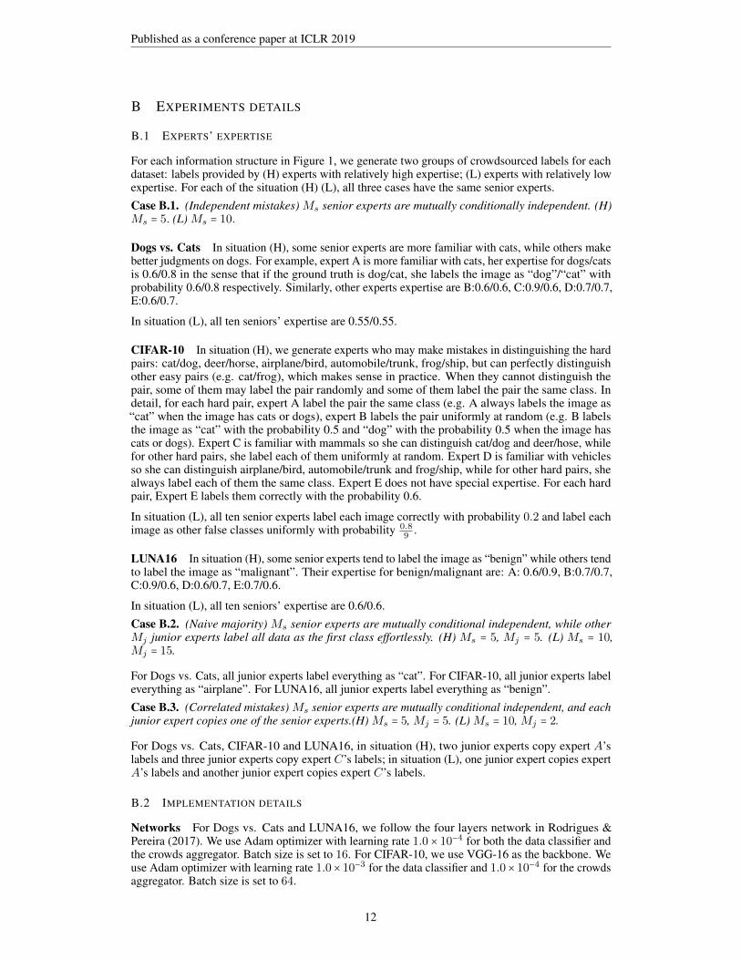
Synthesized crowdsourced labels in various of settings For each information structure in Fig-ure 1, we generate two groups of crowdsourced labels for each dataset: labels provided by (H) expertswith relatively high expertise; (L) experts with relatively low expertise. For each of the situation (H)(L), all three cases have the same senior experts.

Case 4.1. (Independent mistakes) Ms senior experts are mutually conditionally independent.

Case 4.2. (Naive majority) Ms senior experts are mutually conditional independent, while other Mj

junior experts label all datapoints as the first class effortlessly.

Case 4.3. (Correlated mistakes) Ms senior experts are mutually conditional independent, and eachjunior expert copies one of the senior experts.

Real-world dataset The LabelMe data (Rodrigues & Pereira, 2017; Russell et al., 2008) consistsof a total of 2688 images, where 1000 of them were used to obtain labels from multiple annotatorsfrom Amazon Mechanical Turk and the remaining 1688 images were using for evaluating the differentapproaches. Each image was labeled by an average of 2.547 workers, with a mean accuracy of 69.2%.

Networks We follow the four layers network in Rodrigues & Pereira (2017) on Dogs vs. Cats andLUNA16 and use VGG-16 on CIFAR-10 for the backbone of the data classifier h. For Labelme data,we apply the same setting of Rodrigues & Pereira (2017): we use pre-trained VGG-16 deep neuralnetwork and apply only one FC layer (with 128 units and ReLU activations) and one output layer ontop, using 50% dropout.

We defer other implementation details to appendix B.

7


Table 2: Accuracy on LabelMe (real-world crowdsourced labels)

Method Majority Vote Crowd Layer Doctor Net AggNet Max-MIG

Accuracy 80.41 ± 0.56 83.65 ± 0.50 80.56 ± 0.59 85.20 ± 0.26 86.42 ± 0.36

Figure 4: Results on Dogs vs. Cats, CIFAR-10, LUNA16.

4.1 RESULTS

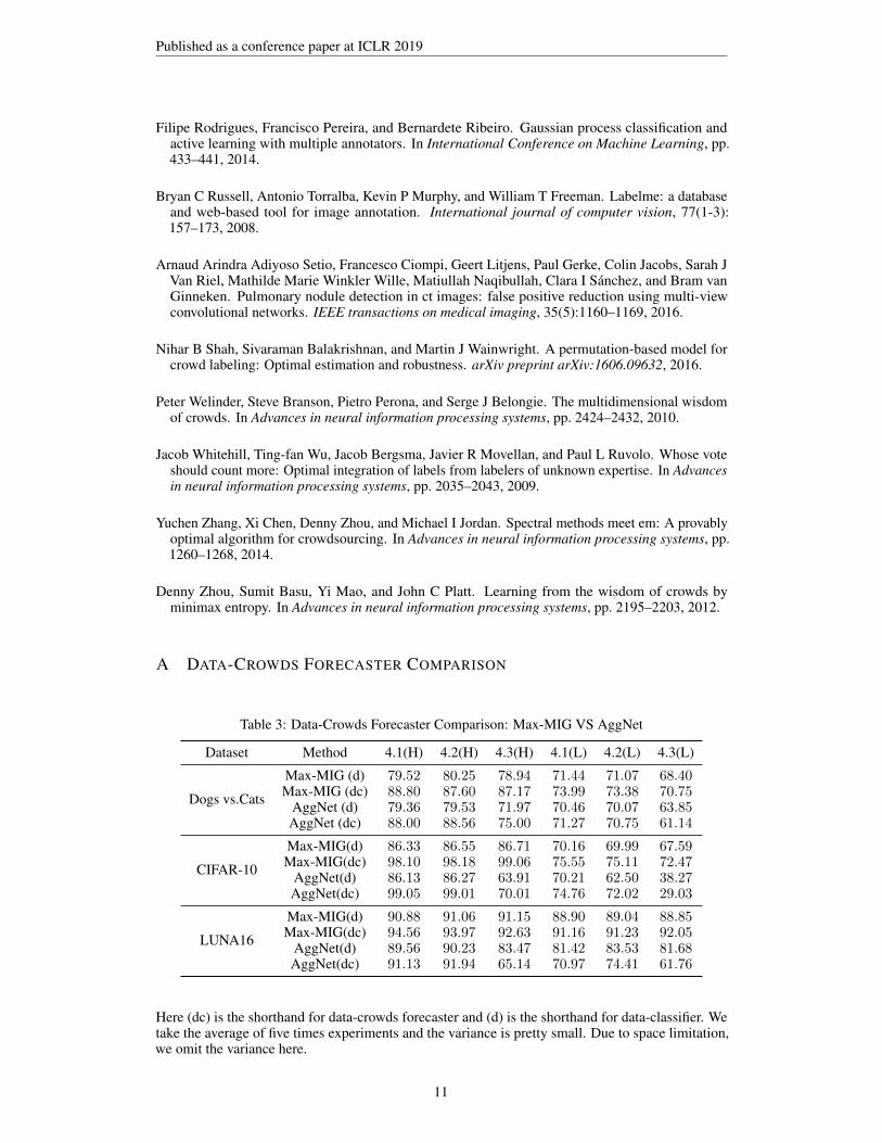
We train the data classifier h on the four datasets through our method1 and other related methods. Theaccuracy of the trained data classifiers on the test set are shown in Table 2 and Figure 4. We also showthe accuracy of our data-crowd forecaster and on the test set and compare it with AggNet (Table 3).

For the performances of the trained data classifiers, our method Max-MIG (red) almost outperformall other methods in every experiment. For the real-world dataset, LabelMe, we achieve the newstate-of-the-art results. For the synthesized crowdsourced labels, the majority vote method (grey)fails in the naive majority situation. The AggNet has reasonably good performances when the expertsare conditionally independent, including the naive majority case since naive expert is independentwith everything, while it is outperformed by us a lot in the correlated mistakes case. This matchesthe theory in Appendix E: the AggNet is based on MLE and MLE fails in correlated mistakes case.The Doctor Net (green) and the Crowd Layer (blue) methods are not robust to the naive majoritycase. Our data-crowds forecaster (Table 3) performs better than our data classifier, which shows thatour data-crowds forecaster actually takes advantage of the additional information, the crowdsourcedlabels, to give a better result. Like us, Aggnet also jointly trains the classifier and the aggregator, andcan be used to train a data-crowds forecaster. We compared our data-crowds forecaster with Aggnet.

1The results of Max-MIG are based on KL divergence. The results for other divergences are similar.

8


The results still match our theory. When there is no correlated mistakes, we outperform Aggnet orhave very similar performances with it. When there are correlated mistakes, we outperform Aggnet alot (e.g. +30%).

Recall that in the experiments, for each of the situation (H) (L), all three cases have the same seniorexperts. Thus, all three cases’ crowdsourced labels have the same amount of information. The resultsshow that Max-MIG has similar performances for all three cases for each of the situation (H) (L),which validates our theoretical result: Max-MIG finds the “information intersection” between thedata and the crowdsourced labels.

5 CONCLUSION AND DISCUSSION

We propose an information theoretic approach, Max-MIG, for joint learning from crowds, witha common assumption: the crowdsourced labels and the data are independent conditioning onthe ground truth. We provide theoretical validation to our approach and compare our approachexperimentally with previous methods (Doctor net (Guan et al., 2017), Crowd layer (Rodrigues &Pereira, 2017), Aggnet (Albarqouni et al., 2016)) under several different information structures. Eachof the previous methods is not robust to at least one information structure and our method is robust toall and almost outperform all other methods in every experiment. To the best of our knowledge, ourapproach is the first algorithm that is both theoretically and empirically robust to the situation wheresome people make highly correlated mistakes and some people label effortlessly, without knowingthe information structure among the crowds. We also test our method on real-world data and achievethe new state-of-the-art result.

Our current implementation of Max-MIG has several limitations. For example, we implement theaggregator using a simple linear model, which cannot handle the case when the senior experts arelatent and cannot be linearly inferred from the junior experts. However, note that if the aggregatorspace is sufficiently rich, the Max-MIG approach is still able to handle any situation as long asthe “information intersection” assumption holds. One potential future direction is designing morecomplicated but still trainable aggregator space.

ACKNOWLEDGMENTS

We would like to express our thanks for support from the following research grants NSFC-61625201and 61527804.

9


REFERENCES

Shadi Albarqouni, Christoph Baur, Felix Achilles, Vasileios Belagiannis, Stefanie Demirci, andNassir Navab. Aggnet: deep learning from crowds for mitosis detection in breast cancer histologyimages. IEEE transactions on medical imaging, 35(5):1313–1321, 2016.

Syed Mumtaz Ali and Samuel D Silvey. A general class of coefficients of divergence of onedistribution from another. Journal of the Royal Statistical Society. Series B (Methodological), pp.131–142, 1966.

Avrim Blum and Tom Mitchell. Combining labeled and unlabeled data with co-training. In Pro-ceedings of the eleventh annual conference on Computational learning theory, pp. 92–100. ACM,1998.

Imre Csiszar, Paul C Shields, et al. Information theory and statistics: A tutorial. Foundations andTrends® in Communications and Information Theory, 1(4):417–528, 2004.

Nilesh Dalvi, Anirban Dasgupta, Ravi Kumar, and Vibhor Rastogi. Aggregating crowdsourced binaryratings. In Proceedings of the 22nd international conference on World Wide Web, pp. 285–294.ACM, 2013.

Alexander Philip Dawid and Allan M Skene. Maximum likelihood estimation of observer error-ratesusing the em algorithm. Applied statistics, pp. 20–28, 1979.

Melody Y Guan, Varun Gulshan, Andrew M Dai, and Geoffrey E Hinton. Who said what: Modelingindividual labelers improves classification. arXiv preprint arXiv:1703.08774, 2017.

Kaggle. Dogs vs. cats competition. https://www.kaggle.com/c/dogs-vs-cats, 2013.

David R Karger, Sewoong Oh, and Devavrat Shah. Budget-optimal task allocation for reliablecrowdsourcing systems. Operations Research, 62(1):1–24, 2014.

Ashish Khetan and Sewoong Oh. Achieving budget-optimality with adaptive schemes in crowdsourc-ing. In Advances in Neural Information Processing Systems, pp. 4844–4852, 2016.

Ashish Khetan, Zachary C Lipton, and Anima Anandkumar. Learning from noisy singly-labeled data.arXiv preprint arXiv:1712.04577, 2017.

Y. Kong and G. Schoenebeck. An Information Theoretic Framework For Designing InformationElicitation Mechanisms That Reward Truth-telling. ArXiv e-prints, May 2016.

Yuqing Kong and Grant Schoenebeck. Water from two rocks: Maximizing the mutual information.In Proceedings of the 2018 ACM Conference on Economics and Computation, pp. 177–194. ACM,2018.

Alex Krizhevsky, Vinod Nair, and Geoffrey Hinton. The cifar-10 dataset. online: http://www. cs.toronto. edu/kriz/cifar. html, 2014.

Qiang Liu, Jian Peng, and Alexander T Ihler. Variational inference for crowdsourcing. In Advancesin neural information processing systems, pp. 692–700, 2012.

Sebastian Nowozin, Botond Cseke, and Ryota Tomioka. f-gan: Training generative neural samplersusing variational divergence minimization. In Advances in Neural Information Processing Systems,pp. 271–279, 2016.

Alexander J Ratner, Christopher M De Sa, Sen Wu, Daniel Selsam, and Christopher Re. Dataprogramming: Creating large training sets, quickly. In Advances in Neural Information ProcessingSystems, pp. 3567–3575, 2016.

Vikas C Raykar, Shipeng Yu, Linda H Zhao, Gerardo Hermosillo Valadez, Charles Florin, LucaBogoni, and Linda Moy. Learning from crowds. Journal of Machine Learning Research, 11(Apr):1297–1322, 2010.

Filipe Rodrigues and Francisco Pereira. Deep learning from crowds. arXiv preprint arXiv:1709.01779,2017.

10


Filipe Rodrigues, Francisco Pereira, and Bernardete Ribeiro. Gaussian process classification andactive learning with multiple annotators. In International Conference on Machine Learning, pp.433–441, 2014.

Bryan C Russell, Antonio Torralba, Kevin P Murphy, and William T Freeman. Labelme: a databaseand web-based tool for image annotation. International journal of computer vision, 77(1-3):157–173, 2008.

Arnaud Arindra Adiyoso Setio, Francesco Ciompi, Geert Litjens, Paul Gerke, Colin Jacobs, Sarah JVan Riel, Mathilde Marie Winkler Wille, Matiullah Naqibullah, Clara I Sanchez, and Bram vanGinneken. Pulmonary nodule detection in ct images: false positive reduction using multi-viewconvolutional networks. IEEE transactions on medical imaging, 35(5):1160–1169, 2016.

Nihar B Shah, Sivaraman Balakrishnan, and Martin J Wainwright. A permutation-based model forcrowd labeling: Optimal estimation and robustness. arXiv preprint arXiv:1606.09632, 2016.

Peter Welinder, Steve Branson, Pietro Perona, and Serge J Belongie. The multidimensional wisdomof crowds. In Advances in neural information processing systems, pp. 2424–2432, 2010.

Jacob Whitehill, Ting-fan Wu, Jacob Bergsma, Javier R Movellan, and Paul L Ruvolo. Whose voteshould count more: Optimal integration of labels from labelers of unknown expertise. In Advancesin neural information processing systems, pp. 2035–2043, 2009.

Yuchen Zhang, Xi Chen, Denny Zhou, and Michael I Jordan. Spectral methods meet em: A provablyoptimal algorithm for crowdsourcing. In Advances in neural information processing systems, pp.1260–1268, 2014.

Denny Zhou, Sumit Basu, Yi Mao, and John C Platt. Learning from the wisdom of crowds byminimax entropy. In Advances in neural information processing systems, pp. 2195–2203, 2012.

A DATA-CROWDS FORECASTER COMPARISON

Table 3: Data-Crowds Forecaster Comparison: Max-MIG VS AggNet

Dataset Method 4.1(H) 4.2(H) 4.3(H) 4.1(L) 4.2(L) 4.3(L)

Dogs vs.Cats

Max-MIG (d) 79.52 80.25 78.94 71.44 71.07 68.40Max-MIG (dc) 88.80 87.60 87.17 73.99 73.38 70.75

AggNet (d) 79.36 79.53 71.97 70.46 70.07 63.85AggNet (dc) 88.00 88.56 75.00 71.27 70.75 61.14

CIFAR-10

Max-MIG(d) 86.33 86.55 86.71 70.16 69.99 67.59Max-MIG(dc) 98.10 98.18 99.06 75.55 75.11 72.47

AggNet(d) 86.13 86.27 63.91 70.21 62.50 38.27AggNet(dc) 99.05 99.01 70.01 74.76 72.02 29.03

LUNA16

Max-MIG(d) 90.88 91.06 91.15 88.90 89.04 88.85Max-MIG(dc) 94.56 93.97 92.63 91.16 91.23 92.05

AggNet(d) 89.56 90.23 83.47 81.42 83.53 81.68AggNet(dc) 91.13 91.94 65.14 70.97 74.41 61.76

Here (dc) is the shorthand for data-crowds forecaster and (d) is the shorthand for data-classifier. Wetake the average of five times experiments and the variance is pretty small. Due to space limitation,we omit the variance here.

11


B EXPERIMENTS DETAILS

B.1 EXPERTS’ EXPERTISE

For each information structure in Figure 1, we generate two groups of crowdsourced labels for eachdataset: labels provided by (H) experts with relatively high expertise; (L) experts with relatively lowexpertise. For each of the situation (H) (L), all three cases have the same senior experts.Case B.1. (Independent mistakes) Ms senior experts are mutually conditionally independent. (H)Ms = 5. (L) Ms = 10.

Dogs vs. Cats In situation (H), some senior experts are more familiar with cats, while others makebetter judgments on dogs. For example, expert A is more familiar with cats, her expertise for dogs/catsis 0.6/0.8 in the sense that if the ground truth is dog/cat, she labels the image as “dog”/“cat” withprobability 0.6/0.8 respectively. Similarly, other experts expertise are B:0.6/0.6, C:0.9/0.6, D:0.7/0.7,E:0.6/0.7.

In situation (L), all ten seniors’ expertise are 0.55/0.55.

CIFAR-10 In situation (H), we generate experts who may make mistakes in distinguishing the hardpairs: cat/dog, deer/horse, airplane/bird, automobile/trunk, frog/ship, but can perfectly distinguishother easy pairs (e.g. cat/frog), which makes sense in practice. When they cannot distinguish thepair, some of them may label the pair randomly and some of them label the pair the same class. Indetail, for each hard pair, expert A label the pair the same class (e.g. A always labels the image as“cat” when the image has cats or dogs), expert B labels the pair uniformly at random (e.g. B labelsthe image as “cat” with the probability 0.5 and “dog” with the probability 0.5 when the image hascats or dogs). Expert C is familiar with mammals so she can distinguish cat/dog and deer/hose, whilefor other hard pairs, she label each of them uniformly at random. Expert D is familiar with vehiclesso she can distinguish airplane/bird, automobile/trunk and frog/ship, while for other hard pairs, shealways label each of them the same class. Expert E does not have special expertise. For each hardpair, Expert E labels them correctly with the probability 0.6.

In situation (L), all ten senior experts label each image correctly with probability 0.2 and label eachimage as other false classes uniformly with probability 0.8

9.

LUNA16 In situation (H), some senior experts tend to label the image as “benign” while others tendto label the image as “malignant”. Their expertise for benign/malignant are: A: 0.6/0.9, B:0.7/0.7,C:0.9/0.6, D:0.6/0.7, E:0.7/0.6.

In situation (L), all ten seniors’ expertise are 0.6/0.6.Case B.2. (Naive majority) Ms senior experts are mutually conditional independent, while otherMj junior experts label all data as the first class effortlessly. (H) Ms = 5, Mj = 5. (L) Ms = 10,Mj = 15.

For Dogs vs. Cats, all junior experts label everything as “cat”. For CIFAR-10, all junior experts labeleverything as “airplane”. For LUNA16, all junior experts label everything as “benign”.Case B.3. (Correlated mistakes) Ms senior experts are mutually conditional independent, and eachjunior expert copies one of the senior experts.(H) Ms = 5, Mj = 5. (L) Ms = 10, Mj = 2.

For Dogs vs. Cats, CIFAR-10 and LUNA16, in situation (H), two junior experts copy expert A’slabels and three junior experts copy expert C’s labels; in situation (L), one junior expert copies expertA’s labels and another junior expert copies expert C’s labels.

B.2 IMPLEMENTATION DETAILS

Networks For Dogs vs. Cats and LUNA16, we follow the four layers network in Rodrigues &Pereira (2017). We use Adam optimizer with learning rate 1.0 × 10−4 for both the data classifier andthe crowds aggregator. Batch size is set to 16. For CIFAR-10, we use VGG-16 as the backbone. Weuse Adam optimizer with learning rate 1.0× 10−3 for the data classifier and 1.0× 10−4 for the crowdsaggregator. Batch size is set to 64.

12


For Labelme data, We apply the same setting of Rodrigues & Pereira (2017): we use pre-trainedVGG-16 deep neural network and apply only one FC layer (with 128 units and ReLU activations) andone output layer on top, using 50% dropout. We use Adam optimizer with learning rate 1.0 × 10−4

for both the data classifier and the crowds aggregator.

For our method MAX-MIG’s crowds aggregator, for Dogs vs. Cats and LUNA16, we set the bias bas logp and only tune p. For CIFAR-10 and Labelme data, we fix the prior distribution p to be theuniform distribution p0 and fix the bias b as logp0.

Initialization For AggNet and our method Max-MIG, we initialize the parameters {Wm}m usingthe method in Raykar et al. (2010):

Wmc,c′ = log

N

∑i=1Q(yi = c)1(ymi = c′)

N

∑i=1Q(yi = c)

(2)

where 1(ymi = c′) = 1 when ymi = c′ and 1(ymi = c′) = 0 when ymi ≠ c′ and N is the total number of

datapoints. We average all crowdsourced labels to obtain Q(yi = c) ∶= 1M

M

∑m=1

1(ymi = c).

For Crowd Layer method, we initialize the weight matrices using identity matrix on Dogs vs. Catsand LUNA as Rodrigues & Pereira (2017) suggest. However, this initialization method leads to prettybad results on CIFAR-10. Thus, we use (2) for Crowd Layer on CIFAR-10, which is the best practicein our experiments.

C f -MUTUAL INFORMATION

C.1 f -DIVERGENCE AND FENCHEL’S DUALITY

f -divergence (Ali & Silvey, 1966; Csiszar et al., 2004) f -divergence Df ∶ ∆Σ ×∆Σ ↦ R is anon-symmetric measure of the difference between distribution p ∈ ∆Σ and distribution q ∈ ∆Σ andis defined to be

Df(p,q) = ∑σ∈Σ

p(σ)f(q(σ)p(σ))

where f ∶ R↦ R is a convex function and f(1) = 0.

C.2 f -MUTUAL INFORMATION

Given two random variables X,Y whose realization space are ΣX and ΣY , let UX,Y and VX,Y betwo probability measures where UX,Y is the joint distribution of (X,Y ) and VX,Y is the product ofthe marginal distributions of X and Y . Formally, for every pair of (x, y) ∈ ΣX ×ΣY ,

UX,Y (X = x,Y = y) = Pr[X = x,Y = y] VX,Y (X = x,Y = y) = Pr[X = x]Pr[Y = y].

If UX,Y is very different from VX,Y , the mutual information between X and Y should be high sinceknowing X changes the belief for Y a lot. If UX,Y equals to VX,Y , the mutual information betweenX and Y should be zero since X is independent with Y . Intuitively, the “distance” between UX,Y

and VX,Y represents the mutual information between them.

Definition C.1 (f -mutual information (Kong & Schoenebeck, 2016)). The f -mutual informationbetween X and Y is defined as

MIf(X,Y ) =Df(UX,Y ,VX,Y )

where Df is f -divergence. f -mutual information is always non-negative.

13


Kong & Schoenebeck (2016) show that if we measure the amount of information by f -mutualinformation, any “data processing” on either of the random variables will decrease the amount ofinformation crossing them. With this property, Kong & Schoenebeck (2016) propose an informationtheoretic mechanism design framework using f -mutual information. Kong & Schoenebeck (2018)reduce the co-training problem to a mechanism design problem and extend the information theoreticframework in Kong & Schoenebeck (2016) to address the co-training problem.

D PROOF OF THEOREM 3.4

This section provides the formal proofs to our main theorem.

Definition D.1 (Confusion matrix). For each expert m, we define her confusion matrix as Cm =(Cmc,c′)c,c′ ∈ R∣C∣×∣C∣ where Cmc,c′ = P (Y m = c′∣Y = c).

We denote the set of all possible classifiers by H∞ and the set of all possible aggregators by G∞.

Lemma D.2. (Kong & Schoenebeck, 2018) With assumption 3.1, 3.3, (h∗, g∗,p∗) is a maximizer of

maxh∈H∞,g∈G∞,p∈∆C


and the maximum is the f mutual information between X and Y [M], MIf(X,Y [M]). Moreover,ζ∗(x, y[M]) = ζ(x, y[M];h∗, g∗,p∗) for every x, y[M].

Proposition D.3. [Independent mistakes] With assumptions 3.1, 3.3, if the experts are mutuallyindependent conditioning on Y , then g∗ ∈ GWA and

g∗(y[M]) = g(y[M];{logCm}Mm=1, logp∗)

for every y[M] ∈ CM .

This implies that (h∗, g∗,p∗) is a maximizer of




Proof. We will show that when the experts are mutually conditionally independent, then

g∗(y[M]) = g(y[M];{logCm}Mm=1, logp∗).

This also implies that g∗ ∈ GWA. Based on the result of Lemma D.2, by assuming that h∗ ∈HNN , we can see (h∗, g∗,p∗) is a maximizer of maxh∈HNN ,g∈GWA,p∈∆CMIGf(h, g,p) and themaximum is the f mutual information between X and Y [M]. Moreover, Lemma D.2 also impliesthat ζ∗(x, y[M]) = ζ(x, y[M];h∗, g∗,p∗) for every x, y[M].

For every c ∈ C, every y[M] ∈ CM ,

(log g∗(y[M]))c = logP (Y = c∣Y [M] = y[M])= logP (Y [M] = y[M]∣Y = c)P (Y = c) − logP (Y [M] = y[M])

=M

∑m=1

logP (Y m = ym∣Y = c) + logP (Y = c) − logP (Y [M] = y[M])

Thus,

(M

∑m=1

logCm ⋅ e(ym) + logp∗)c =

M

∑m=1

logP (Y m = ym∣Y = c) + logP (Y = c)

=(log g∗(y[M]))c + logP (Y [M] = y[M])

14


Then,

(softmax(∑m

logCm ⋅ e(ym) + logp∗))c =

e(log g∗(y[M]))c+logP (Y [M]=y[M])

∑c e(log g∗(y[M]))c+logP (Y [M]=y[M])

= e(log g∗(y[M]))c

∑c e(log g∗(y[M]))c

=(g∗(y[M]))c(since g∗(y[M]) ∈ ∆C , ∑c g∗(y[M])c = 1)

Thus,

g∗(y[M]) = softmax(∑m

logCm ⋅ e(ym) + logp∗) = g(y[M];{logCm}Mm=1, logp∗).

We restate our main theorem, Theorem 3.4, here with more details and prove it.

Theorem 3.4 (General case). With assumption 3.1, 3.3, when there exists a subset of experts S ⊂ [M]such that the experts in S are mutually independent conditioning on Y and Y S is a sufficient statisticfor Y , i.e. P (Y = y∣Y [M] = y[M]) = P (Y = y∣Y S = yS) for every y ∈ C, y[M] ∈ CM , theng∗ ∈ GWA and

g∗(y[M]) = g(y[M];{W∗m}m, logp∗)

for every y[M] ∈ CM where for every m ∈ S, W∗m = logCm, for every m ∉ S, W∗m = 02.

This implies that (h∗, g∗,p∗) is a maximizer of




Proof. Like the proof for the above proposition, we need to show that

g∗(y[M]) = g(y[M];{W∗m}m, logp∗).

This also implies that g∗ ∈ GWA as well as the other results of the theorem.

When Y S is a sufficient statistic for Y , we have

g∗(y[M]) = g∗(yS).

Proposition D.3 shows that

g∗(yS) = g(yS ;{logCs}s∈S , logp∗).

Thus, we have

g∗(y[M]) = g∗(yS) = g(yS ;{logCs}s∈S , logp∗) = g(y[M];{W∗m}m, logp∗)

where for every m ∈ S , W∗m = logCm, for every m ∉ S , W∗m = 0.

2We denote the matrix whose entries are all zero by 0.

15


E THEORETICAL COMPARISONS WITH MLE

Raykar et al. (2010) propose a maximum likelihood estimation (MLE) based method in the learningfrom crowds scenario. Raykar et al. (2010) use logistic regression and Aggnet(Albarqouni et al.,2016) extends it to combine with the deep learning model. In this section, we will theoretically showthat these MLE based methods can handle the independent mistakes case but cannot handle eventhe simplest correlated mistakes case—only one expert reports meaningful information and all otherexperts always report the same meaningless information—which can be handled by our method.Therefore, in addition to the experimental results, theoretically, our method is still better than theseMLE based methods. We first introduce these MLE based methods.

Let Θ be the parameter that control the distribution over X and Y . Let Θm be the parameter thatcontrols the distribution over Y m and Y .

For each each x, y[M],

P (Y [M] = y[M]∣X = x; Θ,{Θm}m) (3)

=∑y

P (Y = y∣X = x; Θ)P (Y [M] = y[M]∣Y = y;{Θm}m)

(conditioning on Y , X and Y [M] are independent)

=∑y

P (Y = y∣X = x; Θ)ΠMm=1P (Y m = ym∣Y = y; Θm)

(experts are mutually conditional independent.)

The MLE based method seeks Θ and Θm that maximize

N

∑i=1

log∑c

P (Y = c∣X = xi; Θ)ΠMm=1P (Y mi = ymi ∣Y = c; Θm)

To theoretically compare it with our method, we use our language to reinterpret the above MLE basedmethod.

We define T as the set of all ∣C∣ × ∣C∣ transition matrices with each row summing to 1.

For each expert m, we define Wm ∈ T as a parameter that is associated with m.

Given a set of data classifiers h ∈ H where h ∶ I ↦ ∆C , the MLE based method seeks h ∈ H andtransition matrices W1,W2,⋯,WM ∈ T that maximize

N

∑i=1

log∑c

h(xi)cΠMm=1W

mc,ymi

.

The expectation of the above formula is

EX,Y [M] log∑c

h(X)cΠMm=1W

mc,Ym .

Note that Raykar et al. (2010) set the data classifiers space H as all logistic regression classifiers andAlbarqouni et al. (2016) extend this space to the neural network space.

Proposition E.1 (MLE works for independent mistakes). If the experts are mutually independentconditioning on Y, then h∗ and C1,C2,⋯,CM are a maximizer of

maxh,W1,W2,⋯,Wm∈T

EX,Y [M] log∑c

h(X)cΠMm=1W

mc,Ym .

16


Proof.

EX,Y [M] log∑c

h(X)cΠMm=1W

mc,Ym

= ∑x,y[M]

P (X = x,Y [M] = y[M]) log∑c

h(x)cΠMm=1W

mc,ym

=∑x

P (X = x) ∑y[M]

P (Y [M] = y[M]∣X = x) log∑c

h(x)cΠMm=1W

mc,ym

Since W1,W2,⋯,Wm ∈ T , thus,

∑y[M]∈CM

∑c∈C

h(x)cΠMm=1W

mc,ym = 1

which means (∑c∈C h(x)cΠMm=1W

mc,ym)y[M] can be seen as a distribution over all possible y[M] ∈ CM .

Moreover, for any two distribution vectors p and q, p ⋅ logq ≤ p ⋅ logp, thus

∑x

P (X = x) ∑y[M]

P (Y [M] = y[M]∣X = x) log∑c

h(x)cΠMm=1W

mc,ym

≤∑x

P (X = x) ∑y[M]

P (Y [M] = y[M]∣X = x) logP (Y [M] = y[M]∣X = x)

=∑x

P (X = x) ∑y[M]

P (Y [M] = y[M]∣X = x) log∑c

h∗(x)cΠMm=1C

mc,Ym (see equation (3))

Thus, the MLE based method handles the independent mistakes case. However, we will constructa counter example to show that it cannot handle a simple correlated mistakes case which can behandled by our method.Example E.2 (A simple correlated mistakes case). We assume there are only two classes C = {0,1}and the prior over Y is uniform, that is, P (Y = 0) = P (Y = 1) = 0.5. We also assume that X = Y .

There are 101 experts and one of the experts, say her the first expert, fully knows Y and alwaysreports Y 1 = Y . The second expert knows nothing and every time flips a random unbiased coin whoserandomness is independent with X,Y . She reports Y 2 = 1 when she gets head and reports Y 2 = 0otherwise. The rest of experts copy the second expert’s answer all the time, i.e. Y m = Y 2, for m ≥ 2.

Note that our method can handle this simple correlated mistakes case and will give all useless expertsweight zero based on Theorem 3.4.

We define h0 as a data classifier such that h0(x)0 = h0(x)1 = 0.5. We will show this meaninglessdata classifier h0 has much higher likelihood than h∗, which shows that in this simple correlatedmistakes case, the MLE based method will obtain meaningless results.

We define a data classifier h’s maximal expected likelihood as

maxW1,W2,⋯,Wm∈T

EX,Y [M] log∑c

h(X)cΠMm=1W

mc,Ym .

Theorem E.3 (MLE fails for correlated mistakes). In the scenario defined by Example E.2, themeaningless classifier h0’s maximal expected likelihood is at least log 0.5 and the Bayesian posteriorclassifier h∗’s maximal expected likelihood is 100 log 0.5 ≪ log 0.5.

The above theorem implies that the MLE based method fails in Example E.2.

Proof. For the Bayesian posterior classifier h∗, since X = Y = Y 1 and Y 2 = ⋯ = YM , thenh∗(X = c) is an one-hot vector where the cth entry is 1 and everything is determined by therealizations of Y and Y 2.

17


EX,Y [M] log∑c

h∗(X)cΠMm=1W

mc,ym

= ∑x,y[M]

P (X = x,Y [M] = y[M]) log∑c

h∗(x)cΠMm=1W

mc,ym

= ∑c,y[M]

P (X = c, Y [M] = y[M]) log∑c

h∗(c)cΠMm=1W

mc,ym

=∑c,c′

P (Y = c)P (Y 2 = c′) logW 1c,cΠ

Mm=2W

mc,c′ (X = Y = Y 1, Y 2 = ⋯ = YM )

=∑c

P (Y = c) logW 1c,c +

M

∑m=2∑c

P (Y = c)∑c′P (Y 2 = c′) logWm

c,c′

≤M

∑m=2∑c

P (Y = c)∑c′P (Y 2 = c′) logWm

c,c′

≤M

∑m=2∑c

P (Y = c)∑c′P (Y 2 = c′) logP (Y 2 = c′)

(Wm is a transition matrix and p ⋅ logq ≤ p ⋅ logp)

=100 log 0.5 (Y 2 equals 0 with probability 0.5 and 1 with probability 0.5 as well)

The maximal value is obtained by setting W1 as an identity matrix and setting W2 = ⋯ = WM

as ( 0.5 0.50.5 0.5

). Thus, the Bayesian posterior data classifier h∗’s maximal expected likelihood is

100 log 0.5. For the meaningless data classifier h0,

EX,Y [M] log∑c

h0(X)cΠMm=1W

mc,ym

= ∑x,y[M]

P (X = x,Y [M] = y[M]) log∑c

h0(x)cΠMm=1W

mc,ym

= ∑x,y[M]

P (X = x,Y [M] = y[M]) log 0.5∑c

ΠMm=1W

mc,ym

=∑c,c′

P (Y = c)P (Y 2 = c′) log 0.5∑c

ΠMm=1W

mc,c′

Note when we set every Wm as an identity matrix, the above formula equals log 0.5. Thus, themeaningless data classifier h0’s maximal expected likelihood is at least log 0.5.

18

M -MIG: INFORMATION THEORETIC APPROACH FOR J L CROWDS

Documents

Transcript of M -MIG: INFORMATION THEORETIC APPROACH FOR J L CROWDS