Lyapunov-based Switched Extremum Seeking

for Photovoltaic Power Maximization

Scott J. Mouraa,∗, Yiyao A. Changb

aMechanical and Aerospace Engineering,University of California, San Diego, CA 92093, USA

bScientific Research & Lead User Programs,National Instruments, Austin TX 78759, USA

Abstract

This paper presents a practical variation of extremum seeking (ES) that guar-antees asymptotic convergence through a Lyapunov-based switching scheme(Lyap-ES). Traditional ES methods enter a limit cycle around the optimum.Lyap-ES converges to the optimum by exponentially decaying the perturba-tion signal once the system enters a neighborhood around the extremum. Asa case study, we consider maximum power point tracking (MPPT) for pho-tovoltaics. Simulation results demonstrate how Lyap-ES is self-optimizing inthe presence of varying environmental conditions and produces greater en-ergy conversion efficiencies than traditional MPPT methods. Experimentallymeasured environmental data is applied to investigate performance under re-alistic operating scenarios.

Keywords: Adaptive control; nonlinear control; Lyapunov methods;photovoltaic systems; renewable energy

1. Introduction

1.1. Problem Statement

Extremum seeking (ES) deals with regulating an unknown system to itsoptimal set-point. To this end, a periodic perturbation signal is typically

∗Tel: +1-858-822-2406; Fax: +1-858-822-3107Email addresses: smoura@ucsd.edu (Scott J. Moura), andy.chang@ni.com (Yiyao

A. Chang)

Preprint submitted to Control Engineering Practice February 19, 2013

used to probe the space. Once the optimal set-point has been identified, mostmethods enter a limit cycle around this point as opposed to converging to itexactly. Hence, one of the main challenges with ES is eliminating the limitcycle and converging to the optimal set-point asymptotically. This paperinvestigates a novel Lyapunov-based switched extremum seeking (Lyap-ES)approach that supplies asymptotic convergence to the optimal set-point. Theproposed concept is demonstrated on a well-studied yet important problem:maximum power point tracking (MPPT) in photovoltaic (PV) systems.

1.2. Literature Review

Two bodies of literature form the foundation of this work: MPPT in PVsand extremum seeking control.

1.2.1. MPPT in PVs

The MPPT literature is extremely broad, and contains techniques thatrange in complexity, hardware, performance, and popularity, among othercharacteristics. The survey paper by Esram and Chapman [1] provides acomprehensive comparative analysis of over 90 publications on MPPT tech-niques. The most popular technique, perturb & observe (P&O), perturbsthe input voltage to determine the direction of the maximum power point(MPP), and moves the operating point accordingly. However, the controllereventually enters a periodic orbit about the MPP. This approach does notrequire a priori knowledge of the PV system and is simple to implement.However, P&O can diverge from the MPP under certain variations in theenvironmental conditions [2], [3]. Recently, an exponentially decaying adap-tive version of P&O has been developed [4], which has conceptual similaritiesto our proposed method. An alternative method, incremental conductance(IncCond), seeks to correct this issue by leveraging the fact that the slopeof PV array power output is zero at the MPP. As a result, this algorithmestimates the slope of the power curve by incrementing the terminal voltageuntil the estimated slope oscillates about zero [5]. A drawback of P&O andIncCond methods is that both stabilize to limit cycles. Ideally, one desiresa peak seeking scheme that is asymptotically convergent and self-optimizingwith respect to shifts in the MPP. This motivates a control-theoretic ap-proach to MPPT. A recent paper examined an adaptive backstepping ap-proach, for which convergence to the MPP is theoretically proven under apersistency of excitation condition [6]. This paper examines an alternativenon-model-based approach, extremum seeking.

2

Extremum seeking control and its application to photovoltaic systems rep-resents an important and relevant subset of MPPT literature. Specifically,Leyva et al. [7] and Bratcu et al. [8] utilize extremum seeking for PVs byinjecting an exogenous periodic signal. A separate research group developedripple correlation control (RCC), which utilizes the signal ripple that inher-ently exists in systems with switching power electronics as the perturbationsignal [9]. The stability and optimality of this approach has been establishedin [10]. RCC has the critical advantage of utilizing existing signal ripples, in-stead of injecting artificial perturbations. As such, RCC is only applicable tosystems which inherently contain ripple characteristics. Recently, Brunton etal. [11] utilized the 120 Hz inverter ripple in a PV system within the contextof an extremum seeking control theoretic approach to MPPT. Consequentlythis work established an important link between extremum seeking controland ripple-based MPPT [12].

1.2.2. Extremum Seeking Control Theory

Prior to the nonlinear and adaptive control theory developments in the1970’s and 1980’s, extremum seeking was proposed as a method for identi-fying the optimum of an equilibrium map. Since then, researchers have ex-tended extremum seeking to the general class of nonlinear dynamical plants(see e.g. [13], [14]) and applied the algorithm to a wide variety of applica-tions (e.g. air flow control in fuel cells [15], wind turbine energy capture [16],ABS control, and bioreactors [17]). During this period there have been sev-eral innovations that have improved the practicability of ES. For example,convergence speed can be enhanced by adding dynamic compensators [18]or applying alternative periodic perturbation signals [19]. A Newton-basedalgorithm can also be developed by estimating the Hessian of the unknownnonlinear map [20].

1.3. Contributions

This study focuses on a general problem - asymptotic convergence tothe extremum of a static nonlinear unknown function. As such, this paperextends the aforementioned research and builds on the authors’ previous work[21] to add the following two new contributions to the ES control and MPPTbodies of literature. First, we introduce a switching method for ensuringasymptotic convergence to the optimal operating point, based on Lyapunovstability theory. Secondly, we demonstrate this algorithm in simulation for

3

MPPT problems in PV systems - a novel and control theoretic alternative totraditional MPPT methods.

1.4. Paper Outline

This paper is organized as follows: Section 2 describes the extremum seek-ing control design and our novel Lyapunov-based switching strategy. Section3 discusses a case study of the proposed ES method on MPPT for PV sys-tems. Finally, Section 4 presents the main conclusions.

2. Extremum Seeking Control

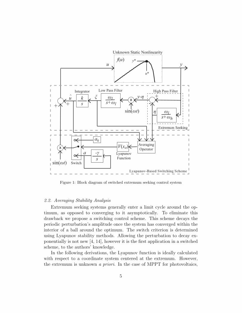
In this section we introduce and expand upon a simple yet widely studiedextremum seeking (ES) scheme [13], [17] for static nonlinear maps, shown inFig. 1. Since the case study on photovoltaic systems involves a static plantmodel (albeit parameterized by time-varying disturbances), the scope of ouranalysis is limited to static plants. One may also consider the more generalsingular perturbation analysis for dynamic plant models presented in [13].

Before embarking on a detailed discussion of this method, we give anintuitive explanation of how extremum seeking works, which can also befound in [13] and [17], but is presented here for completeness. Next, wedesign the Lyapunov-based switching extremum seeking control to eliminatelimit cycles.

2.1. An Intuitive Explanation

The control scheme applies a period perturbation a0 sin(ωt) to the controlsignal u, whose value estimates the optimal control input u∗. This controlinput passes through the unknown static nonlinearity f(u + a0sin(ωt)) toproduce a periodic output signal y. The high-pass filter s/(s + ωh) theneliminates the DC components of y, and will be in or out of phase with theperturbation signal a0 sin(ωt) if u is less than or greater than u∗, respectively.This property is important because when the signal y − η is multiplied bythe perturbation signal sin(ωt), the resulting signal has a DC componentgreater than or less than zero if u is less than or greater than u∗, respec-tively. This DC component is extracted by the low-pass filter ωl/(s + ωl)

and represents the sensitivity (a202

)∂f∂u

(u). We may use a gradient update law˙u = k(

a202

)∂f∂u

(u) or a quasi-Newton method [22] to force u to converge to u∗.Next we rigorously develop the ES algorithm.

4

s+ωh

ωls+ωl

ks

x

Unknown Static Nonlinearity

f(u)

sin(ωt)

sin(ωt)

u y

y-ηξu^

y*

u*

Integrator Low Pass Filter

+ +

x

a0

-γs

V(xa)LyapunovFunction

Switch

a

Extremum Seeking

Lyapunov-Based Switching Scheme

Extremum SeekingExtremum Seeking

AveragingOperator

ωl

-+

η

High Pass Filter

Figure 1: Block diagram of switched extremum seeking control system

2.2. Averaging Stability Analysis

Extremum seeking systems generally enter a limit cycle around the op-timum, as opposed to converging to it asymptotically. To eliminate thisdrawback we propose a switching control scheme. This scheme decays theperiodic perturbation’s amplitude once the system has converged within theinterior of a ball around the optimum. The switch criterion is determinedusing Lyapunov stability methods. Allowing the perturbation to decay ex-ponentially is not new [4, 14], however it is the first application in a switchedscheme, to the authors’ knowledge.

In the following derivations, the Lyapunov function is ideally calculatedwith respect to a coordinate system centered at the extremum. However,the extremum is unknown a priori. In the case of MPPT for photovoltaics,

5

we assume knowledge of a “nominal” MPP, provided by the manufacturerunder ideal conditions. The Lyapunov function will be evaluated with respectto a coordinate system centered at this nominal extremum. An analysis inSection 3.4 evaluates the impact of errors between the nominal and trueextrema.

We start with a proof modified from Krstic and Wang [13], which usesaveraging theory to approximate the ES system behavior, linearizes it aboutthe equilibrium, and then shows the resulting Jacobian is Hurwitz. From thisproof, our new contribution is to develop a Lyapunov function that sensesproximity to the equilibrium point.

The state equations for the closed-loop ES system are:

˙u = kξ (1)

ξ = −ωlξ − ωlη sin(ωt) + ωlf(u)sin(ωt) (2)

η = −ωhη + ωhf(u) (3)

u = u+ a0sin(ωt) (4)

where each equation respectively represents the integrator, low-pass filter,high-pass filter, and perturbed control input. Now define a new coordinatesystem that shifts the nominal optimal operating point, denoted u0, to theorigin

u = u− u0 (5)

η = η − f(u0) (6)

resulting in the following translated system

˙u = kξ (7)

ξ = −ωlξ − ωlη sin(ωt)

+ ωl[f(u+ u0 + a0 sin(ωt)− f(u0)

](8)

˙η = −ωhη − ωh[f(u+ u0 + a0 sin(ωt))− f(u0)

](9)

Now we scale time τ = ωt.

d

dτ

uξη

= δ

K ′ξ−ω′Lξ − ω′Lη sin(τ) + ω′Lh(u+ a0 sin τ) sin τ

−ω′H η − ω′Hh(u+ a0 sin(ωt))

6

where the parameters are normalized as follows:

k = ωδK′= O(ωδ) (10)

ωl = ωδω′L = O(ωδ) (11)

ωh = ωδω′H = O(ωδ) (12)

and K ′, ω′L, ω′H are O(1) positive constants. The function h(θ) = f(u0 + θ)−

f(u0) satisfies the following properties in photovoltaic systems.

h(0) = 0 (13)

h′(0) = f ′(u0) (14)

h′′(0) = f ′′(u0) < 0 (15)

h′′′(0) = f ′′′(u0) < 0 (16)

These properties will be useful in our calculations later. Also note that (14)is equal to zero when the u0 = u∗.

To investigate the stability properties of this system, we consider theaveraged system - the standard approach for analyzing periodic systems.The averaged state variables are defined as follows [20].

xa =1

2π

∫ τ

τ−2πx(σ)dσ (17)

where the period of the signal is 2π. Hence, our immediate goal is to usethe notion of an averaged system to investigate the stability properties of theclosed loop system. Applying the definition of averaging yields the followingsystem

d

dτ

uaξaηa

= δ

K ′ξa

−ω′Lξa +ω′L

2π

∫ 2π

0h(ua + a0 sinσ) sinσdσ

−ω′H ηa +ω′H

2π

∫ 2π

0h(ua + a0 sinσ)dσ

(18)

Now we must determine the equilibrium (uea, ξea, η

ea) of this nonlinear system

which satisfies:

0 =

K ′ξea−ω′Lξea +

ω′L

2π

∫ 2π

0h(uea + a0 sinσ) sinσdσ

−ω′H ηea +ω′H

2π

∫ 2π

0h(uea + a0 sinσ)dσ

(19)

7

Let us postulate that uea takes the form uea = b1a0 + b2a20 + O(a30) and use

a Maclaurin series expansion of h(uea + a0 sinσ). Following several algebraiccalculations that use (13)-(16), one may show the equilibrium is given by:

uea = b0 −h′′′(0)

h′′(0) + b0h′′′(0)a20 +O(a30) (20)

where b0 solves h′′′(0)b20 + 4h′′(0)b0 + 2h′(0) = 0.

ξea = 0 (21)

ηea = h′(0)b0 + h′′(0)b20 +1

6h′′′(0)b30 +

[h′(0)b2 +

1

4h′′(0)

+ 2b0b2h′′(0) +

1

4b0h′′′(0) +

1

2b20b2h

′′′(0)

]a20 +O(a30) (22)

and b2 = −h′′′(0)/ (h′′(0) + b0h′′′(0)).

The Jacobian of (18) evaluated at (uea, ξea, η

ea) is

Ja = δ

0 K ′ 0ω′L

2π

∫ 2π

0h′(uea + a0 sinσ) sinσdσ −ω′L 0

ω′H

2π

∫ 2π

0h′(uea + a0 sinσ)dσ 0 −ω′H

(23)

Inspection reveals the Jacobian has a block-lower-triangular structure. As aresult, Ja is Hurwitz if and only if∫ 2π

0

h′(uea + a0 sinσ) sinσdσ < 0 (24)

We apply (13)-(16) to show that∫ 2π

0

h′(uea + a0 sinσ) sinσdσ = πh′′(0)a0 +O(a20) (25)

Using the property (15), we conclude the Jacobian is Hurwitz for sufficientlysmall a0. Since the Jacobian is Hurwitz, the averaged system is locally expo-nentially stable according to Theorem 4.7 of Khalil [23]. This also satisfiesthe conditions of Theorem 10.4 of Khalil [23], which states that the originalsystem has a unique exponentially stable periodic orbit about (uea, ξ

ea, η

ea).

Therefore the ES control system is stable in the sense that the averaged sys-tem converges exponentially for sufficiently small a0. We leverage this factto design the Lyapunov-based switching criterion, described next.

8

2.3. Lyapunov-Based Switching Scheme

The Jacobian (23) approximates the system dynamics near the equilib-rium (uea, ξ

ea, η

ea). We now use this Jacobian to develop a quadratic Lyapunov

function for the switching control. First, we use (25) and similar calculations

for∫ 2π

0h′(uea + a0 sinσ)dσ to write the Jacobian as:

Ja = δ

0 K ′ 0ω′L

2h′′(0)a0 −ω′L 0

ω′Hh′(0) 0 −ω′H

(26)

where we use estimates for h′(0) & h′′(0) which satisfy (14)-(15). Next wesolve the following Lyapunov equation for P

PJa + JTa P = −Q (27)

which has a unique solution under the conditions Q = QT > 0. This resultsin the following quadratic Lyapunov function

V (xa) =1

2xTaPxa where xa = [ua ξa ηa]

T (28)

which we use for the following switched control law:

u(t) =

u+ a0sin(ωt) if V (xa) > εu+ asin(ωt)

da(t)dt

= −ρa(t), a(0) = a0 otherwise

(29)

whose conditions are evaluated only when sin(ωt) equals zero to ensure thecontrol signal remains continuous in time.

Remark 1 (ES Re-engagement Property). The quadratic Lyapunov func-tion in (28) estimates the averaged system’s proximity to the equilibrium.That is, V (xa)→ 0 as xa → 0. Once Lyap-ES converges sufficiently close tothe optimum, the sinusoidal perturbation decays exponentially to zero andthe control input arrives at u∗. If external disturbances cause the Lyapunovfunction value to increase above the threshold value ε, then the original am-plitude a0 is used until the system converges to the new extremum. Hence,the proposed switched control scheme is self-optimizing with respect to dis-turbances. This situation is illustrated in the case study on PV systems inSection 3.

9

Remark 2 (Positive Invariance Property). Note that the sub-level set Ωc =xa ∈ R3 | V (xa) ≤ c which V (xa) ≤ 0 is positively invariant, mean-ing a solution starting in Ωc remains in Ωc for all t ≥ 0. In other words,the Lyapunov function will be decreasing monotonically in time, thereforeeliminating chattering behavior.

Remark 3 (Convergence Speed). During the case of constant perturba-tion amplitude, the convergence speed to the invariant set Ωε = xa ∈R3|V (xa) ≤ ε is characterized by the eigenvalues of (26). Once the per-turbation amplitude switches to an exponential decay, the convergence ischaracterized by the decay parameter ρ in (29). In practice, one would usethe algorithm parameters to compute convergence speeds from these rela-tions.

Although we refrain from stating theorems and proofs in this paper, sta-bility can be established by considering three points. First, the dynamics ofa, which are in a cascade with the ES dynamics, are trivially stable. Second,u(t) is continuous across the switching times since the conditions of (29) areevaluated only when sin(ωt) = 0. Given these two points, stability of thecomplete closed-loop system can be established by studying the ES dynam-ics augmented with the decaying amplitude state in (29). Unfortunately, thelinearization test applied in [13] fails in this case because the Jacobian con-tains a zero eigenvalue. However, it may be possible to use an appropriatelyselected Lyapunov function or the Center Manifold Theorem (Section 8.1 of[23]) to prove local asymptotic stability.

3. Case Study: MPPT In Photovoltaic Systems

Next we examine the proposed Lyapunov-based switched extremum seek-ing scheme on the MPPT problem for PV systems. Solar energy representsa key opportunity for increasing the role of renewable energy in the electricgrid. However, high manufacturing and installation costs have limited theeconomic viability of PV-based energy production [24]. Therefore, it is vi-tally important to maximize the energy conversion efficiency of PV arrays.This problem is particularly difficult because maximizing energy capture inPVs can depend on varying incident solar radiation, temperature, shading,system degradation, etc. As such, we desire control theoretic techniquesthat mathematically guarantee asymptotic convergence to the MPP, whilerejecting disturbances due to changing environments.

10

DC/DC

Converter

Switched ES

MPPT Control

PV Array

Voltage

& current

measurements

PWM control

Solar irradiation

& temperature

disturbances

to DC/AC

inverter

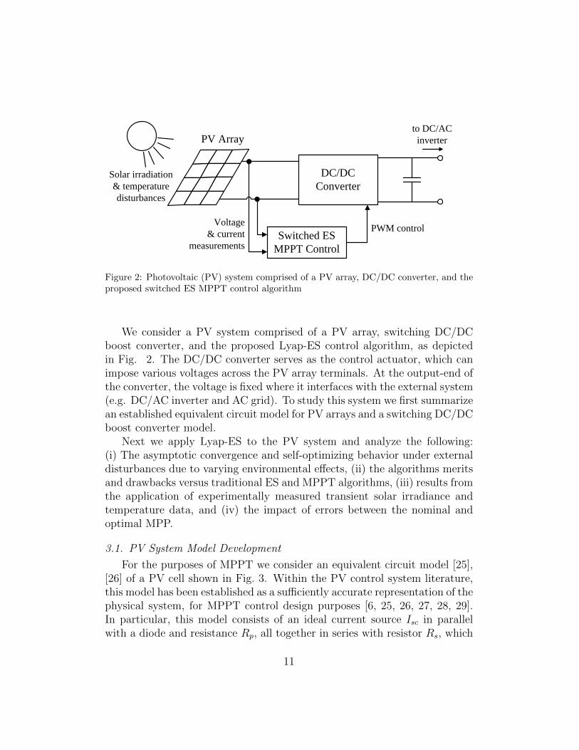
Figure 2: Photovoltaic (PV) system comprised of a PV array, DC/DC converter, and theproposed switched ES MPPT control algorithm

We consider a PV system comprised of a PV array, switching DC/DCboost converter, and the proposed Lyap-ES control algorithm, as depictedin Fig. 2. The DC/DC converter serves as the control actuator, which canimpose various voltages across the PV array terminals. At the output-end ofthe converter, the voltage is fixed where it interfaces with the external system(e.g. DC/AC inverter and AC grid). To study this system we first summarizean established equivalent circuit model for PV arrays and a switching DC/DCboost converter model.

Next we apply Lyap-ES to the PV system and analyze the following:(i) The asymptotic convergence and self-optimizing behavior under externaldisturbances due to varying environmental effects, (ii) the algorithms meritsand drawbacks versus traditional ES and MPPT algorithms, (iii) results fromthe application of experimentally measured transient solar irradiance andtemperature data, and (iv) the impact of errors between the nominal andoptimal MPP.

3.1. PV System Model Development

For the purposes of MPPT we consider an equivalent circuit model [25],[26] of a PV cell shown in Fig. 3. Within the PV control system literature,this model has been established as a sufficiently accurate representation of thephysical system, for MPPT control design purposes [6, 25, 26, 27, 28, 29].In particular, this model consists of an ideal current source Isc in parallelwith a diode and resistance Rp, all together in series with resistor Rs, which

11

Isc Vd

+

-

Rp

Rs

Vcell

+

-

I

S

Figure 3: Equivalent circuit model of PV Cell [25], [26]

models contactor and semiconductor material resistance. The ideal currentsource delivers current in proportion to solar flux S, and is also a function oftemperature T . The diode models the effects of the semiconductor material,and also depends on temperature. In total, the PV cell model equations aregiven by

Vd = Vcell + IRs (30)

I = Isc − I0[exp

(qVdAkT

)− 1

]− VdRp

(31)

Isc = [Isc,r + kI(T − Tr)]S

1000(32)

I0 = I0,r

(T

Tr

)3

exp

[qESiAk

(1

Tr− 1

T

)](33)

Vpv = ncellVcell (34)

The cell model is scaled to an array by considering ncell cells in series(34). Parameters are adopted from [25].

The PV model is parameterized by environmental conditions - incidentsolar irradiation S and temperature T . Figure 4 demonstrates that currentand power increase linearly with solar irradiation. Temperature has a morecomplex effect on current and power. The short circuit current increaseswith temperature, however the power decreases as temperature increases.

12

Consequently, PV cells operate best in full sunlight and cold temperatures.Our goal is to design a control loop that automatically tracks the MPP underchanging environments.

A DC/DC boost converter steps up the PV array voltage and providesa control actuator for MPPT, via PWM on the switches. At the boost con-verter’s output, a capacitor maintains a roughly constant voltage and is typ-ically interfaced with the electric grid using a three-phase DC/AC inverter[2]. In this paper, we focus on the boost converter only for the purposesof MPPT, and assume the capacitor maintains a constant 120V at the out-put. In the following, we analyze the dynamics of a switching DC/DC boostconverter model. Namely, we find the equilibrium of this system and showthat it is locally exponentially stable. This analysis enables us to use theequilibrium as a reduced DC/DC model for the purposes of MPPT.

Cur

rent

[A]

3

0

0.5

1

1.5

2

2.5

300 2 4 6 8 10 12 14 16 18 20 22 24 26 28

20 ºC

40 ºC

60 ºC

80 ºC

0 ºCC

urre

nt [A

]3

0

0.5

1

1.5

2

2.5

300 2 4 6 8 10 12 14 16 18 20 22 24 26 28

600 W/m²

800 W/m²

1k W/m²

200 W/m²

400 W/m²

Powe

r [W

]

50

0

5

10

15

20

25

30

35

40

45

Voltage [V]300 2 4 6 8 10 12 14 16 18 20 22 24 26 28

Powe

r [W

]

50

0

5

10

15

20

25

30

35

40

45

Voltage [V]300 2 4 6 8 10 12 14 16 18 20 22 24 26 28

Figure 4: Characteristic I-V and P-V curves for varying T and S = 1000 W/m2 (leftsubplots), and varying S and T = 25C (right subplots).

Figure 5 provides a schematic of a typical switching DC/DC boost con-verter. The input side interfaces with the PV array, represented by the static

13

±

±

+

-

q

L

C

R

Vinv

vc

iL

+

-

Vpv

(iL; S,T)

Figure 5: Circuit diagram of switching DC/DC boost converter model.

relation Vpv(I;S, T ) which verifies (30)-(34). The output side interfaces witha DC/AC inverter, which is modeled as a fixed voltage source Vinv and equiv-alent series resistance. The dynamics of this switched system, after applyingthe state-space averaging approach [30], are:

d

dtiL =

1

LVpv(iL;S, T )− 1− d

Lvc (35)

d

dtvc =

1− dC

iL −1

RC(vc − Vinv) (36)

where d ∈ (0, 1) is the duty ratio. The equilibrium for this nonlinear system(ieqL , v

eqc ) satisfies:

veqc = (1− d)RieqL + Vinv (37)

0 = Vpv(ieqL ;S, T )− (1− d)2RieqL − (1− d)Vinv (38)

Now we analyze the stability of this equilibrium. First, we linearize (35)-(36) around (ieqL , v

eqc ), producing the Jacobian[

1L

∂Vpv∂iL

(ieqL ;S, T ) −(1− d) 1L

(1− d) 1C

− 1RC

](39)

The eigenvalues λ of (39) satisfy the characteristic equation:

0 = λ2 +

[1

RC− 1

L

∂Vpv∂iL

(ieqL ;S, T )

]λ

− 1

RLC

∂Vpv∂iL

(ieqL ;S, T ) + (1− d)21

LC(40)

14

0 5 10 15 20 250

0.5

1

1.5

2

2.5

3

Cu

rre

nt [A

]

Characteristic Curve

ES Trajectory

Initial Operating Point

Converged Solution

Maximum Power Point

0 5 10 15 20 250

10

20

30

40

Po

we

r [W

]

Voltage [V]

Figure 6: Trajectories of current and power on PV array characteristic curves for 1000W/m2 to 500 W/m2 step change in solar irradiation.

Observe that ∂Vpv/∂iL(ieqL ;S, T ) < 0 over its entire domain, for all physicallymeaningful values of S, T . Therefore, all the coefficients of λ in (40) arepositive. By the Routh-Hurwitz stability criterion, Re[λ] < 0. Consequently,the equilibrium (ieqL , v

eqc ) is locally exponentially stable.

For the proposed MPPT algorithm, we impose the condition that theswitching converter dynamics are notably faster than the Lyap-ES loop dy-namics. This enables us to use the stable equilibrium to model the DC/DCboost converter dynamics as:

0 = Vpv(I;S, T )− (1− d)2RI − (1− d)Vinv (41)

where Vpv is the PV array voltage, Vinv is the constant 120V DC/AC invertervoltage, and d is the duty ratio control input.

15

3.2. Concept Demonstration

In this section we demonstrate Lyap-ES by (i) analyzing the impact ofvarying environmental conditions, and (ii) comparing it to P&O and tradi-tional ES methods. In the first part we impose 1000 W/m2 of solar irradiationand then provide a 500 W/m2 step change at 200 ms. This might model thetransient effect of a passing cloud blocking incident sunlight. The duty ratiois initialized at 0.9. The control parameters for Lyap-ES are provided inTable 1. Remarks on control parameter selection are included in AppendixA.

3.2.1. Impact of Varying Environmental Conditions

Figure 6 demonstrates the current and power trajectories superimposedon the PV array’s characteristic I-V and P-V curves (S = 1000 W/m2).Lyap-ES indeed achieves the maximum power of 38W at voltage and currentvalues of 17V and 2.24A for S = 1000 W/m2, and maximum power of 17.3Wat voltage and current values of 18V and 1.09A for S = 500 W/m2. Moreover,one can see how the operating point jumps from the 1000 W/m2 characteristiccurve to the 500 W/m2 curve during the step change. Immediately after thestep change, the operating point is no longer at the MPP. The algorithmsenses this change and reengages the perturbation to find the new MPP.

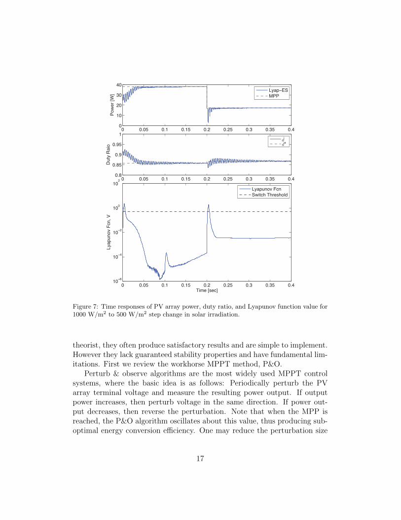
Time responses of power, duty ratio, and Lyapunov function value areprovided in Figure 7. This figure demonstrates how Lyap-ES injects sinu-soidal perturbations into the duty ratio to determine the MPP u∗ = 0.859for S = 1000 W/m2 and 0.868 for S = 500 W/m2. Note the perturbationsbegin to decay exponentially at 7.5 ms and u(t) converges to u∗. Once theirradiation changes at 200 ms, the perturbation re-engages to search for thenew MPP. Once it converges sufficiently close to the optimal duty ratio, theperturbation amplitude decays exponentially once again.

The switch behavior can be understood by analyzing Figure 7. At 7.5ms, V (xa) < ε and the perturbation decays. Once the solar flux step changeoccurs at 200 ms, the averaged states become excited and V (xa) > ε. Thisresets the amplitude of the perturbation to a0. Then, as V (xa) < ε, theperturbation amplitude decays exponentially once again.

3.2.2. Comparative Analysis to Existing Methods

This section compares Lyap-ES to standard ES and a traditional MPPTtechnique: perturb & observe [2], [3] (P&O). Although some traditionalMPPT methods are somewhat heuristic and may not appeal to the control

16

0 0.05 0.1 0.15 0.2 0.25 0.3 0.35 0.410

−6

10−4

10−2

100

102

Lyapunov Fcn, V

Time [sec]

Lyapunov Fcn

Switch Threshold

0 0.05 0.1 0.15 0.2 0.25 0.3 0.35 0.40.8

0.85

0.9

0.95

1

Duty Raio

dd

0 0.05 0.1 0.15 0.2 0.25 0.3 0.35 0.40

10

20

30

40

Power [W

]

Lyap−ES

MPP

*

Figure 7: Time responses of PV array power, duty ratio, and Lyapunov function value for1000 W/m2 to 500 W/m2 step change in solar irradiation.

theorist, they often produce satisfactory results and are simple to implement.However they lack guaranteed stability properties and have fundamental lim-itations. First we review the workhorse MPPT method, P&O.

Perturb & observe algorithms are the most widely used MPPT controlsystems, where the basic idea is as follows: Periodically perturb the PVarray terminal voltage and measure the resulting power output. If outputpower increases, then perturb voltage in the same direction. If power out-put decreases, then reverse the perturbation. Note that when the MPP isreached, the P&O algorithm oscillates about this value, thus producing sub-optimal energy conversion efficiency. One may reduce the perturbation size

17

Table 1: Lyap-ES Controller Parameters.

Symbol Description Concept Demon-stration Study

ExperimentalData Study

u0Duty ratio for nominal MPP

0.859 0.859@ 1000W/m2, 25C

ω Perturbation frequency 250 Hz 0.2 Hzωh High-pass filter cut-off freq. 50 Hz 0.04 Hzωl Low-pass filter cut-off freq. 50 Hz 0.04 Hza0 Perturbation amplitude 0.015 0.01k Gradient update law gain 1 0.0008ε Lyap. Fcn. Threshold 0.01 20

γ Perturbation amplitude 50 0.1decay rate

σ2P Variance of measured 0 W 0.2 W

power noise

to improve efficiency during steady-state, but this reduces convergence speed.Moreover, P&O cannot differentiate if a power increase is due to the voltageperturbation or a disturbance. An increase in solar irradiation or drop intemperature will confuse the P&O algorithm.

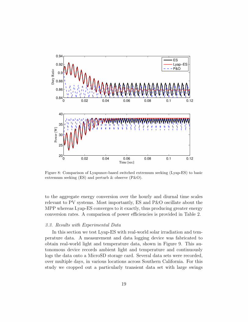
Figure 8 compares Lyap-ES to two benchmarks: P&O and basic ES (si-nusoidal perturbation with no switching). The simulated conditions are iden-tical to the previous subsection, however we do not consider varying incidentsolar irradiation. The perturbation amplitude and frequency of P&O are setequal to the Lyap-ES parameter values of a0 and ω, respectively, to providecomparable results.

Several key observations arise from this study. First, ES and Lyap-ESare identical for the first 40ms. Afterwards, the switch condition is satisfiedand Lyap-ES converges to u∗. Consequently, the power output from Lyap-ES upper-bounds the other algorithms. Secondly, although P&O convergesfaster than Lyap-ES, for the parameters considered here, the average out-put power is less than ES or Lyap-ES. Alternative parameter choices for ESand Lyap-ES can increase convergence speed (using the relations describedin Remark 3), but may create bias induced from the high order harmonicsthat are insufficiently attenuated by the low pass filter. Ultimately, differ-ences in convergence on the order of 10s of milliseconds are trivial compared

18

0 0.02 0.04 0.06 0.08 0.1 0.120.84

0.86

0.88

0.9

0.92

0.94D

uty

Rat

io

ES

Lyap−ES

P&O

0 0.02 0.04 0.06 0.08 0.1 0.1220

25

30

35

40

Po

wer

[W

]

Time [sec]

Figure 8: Comparison of Lyapunov-based switched extremum seeking (Lyap-ES) to basicextremum seeking (ES) and perturb & observe (P&O).

to the aggregate energy conversion over the hourly and diurnal time scalesrelevant to PV systems. Most importantly, ES and P&O oscillate about theMPP whereas Lyap-ES converges to it exactly, thus producing greater energyconversion rates. A comparison of power efficiencies is provided in Table 2.

3.3. Results with Experimental Data

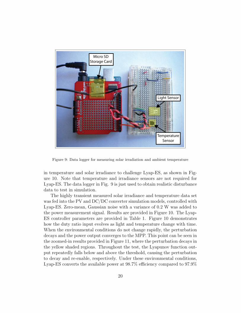
In this section we test Lyap-ES with real-world solar irradiation and tem-perature data. A measurement and data logging device was fabricated toobtain real-world light and temperature data, shown in Figure 9. This au-tonomous device records ambient light and temperature and continuouslylogs the data onto a MicroSD storage card. Several data sets were recorded,over multiple days, in various locations across Southern California. For thisstudy we cropped out a particularly transient data set with large swings

19

Micro SD

Storage Card

Light Sensor

Temperature

Sensor

Figure 9: Data logger for measuring solar irradiation and ambient temperature

in temperature and solar irradiance to challenge Lyap-ES, as shown in Fig-ure 10. Note that temperature and irradiance sensors are not required forLyap-ES. The data logger in Fig. 9 is just used to obtain realistic disturbancedata to test in simulation.

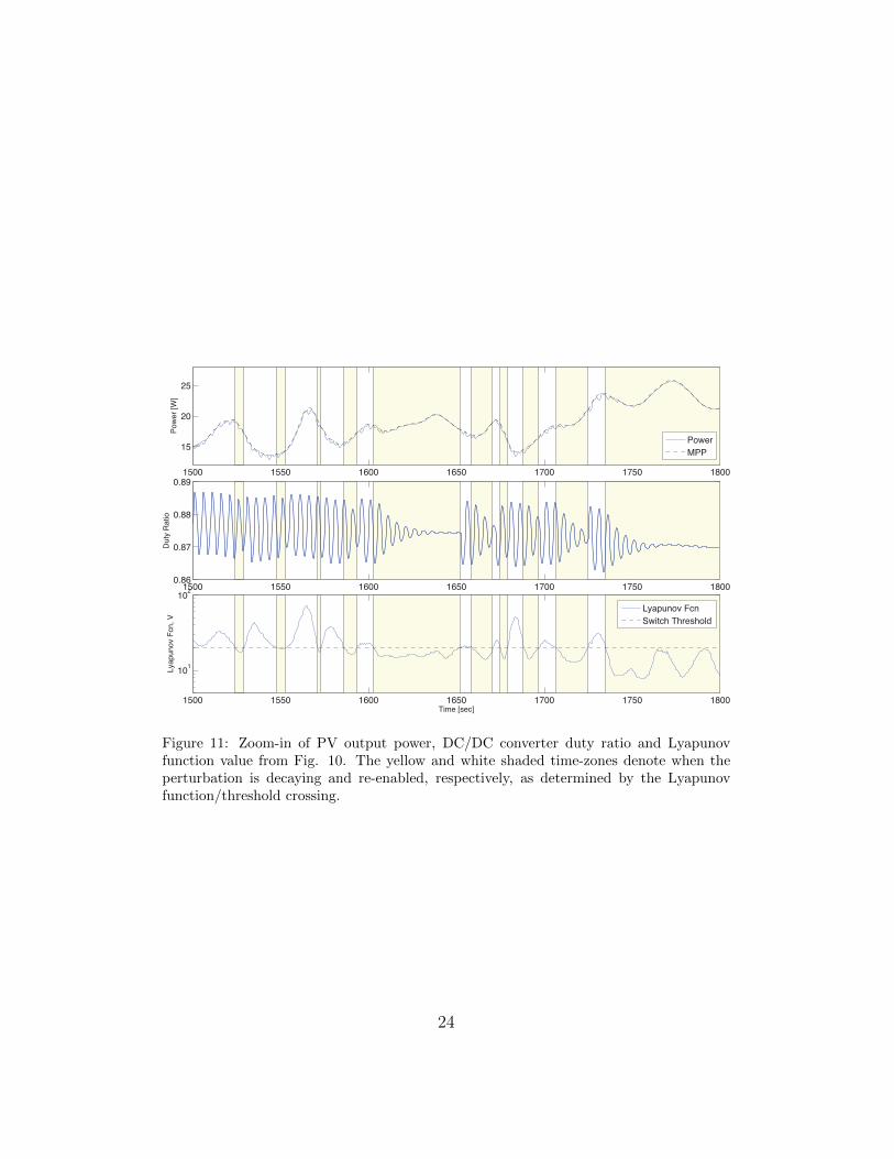
The highly transient measured solar irradiance and temperature data setwas fed into the PV and DC/DC converter simulation models, controlled withLyap-ES. Zero-mean, Gaussian noise with a variance of 0.2 W was added tothe power measurement signal. Results are provided in Figure 10. The Lyap-ES controller parameters are provided in Table 1. Figure 10 demonstrateshow the duty ratio input evolves as light and temperature change with time.When the environmental conditions do not change rapidly, the perturbationdecays and the power output converges to the MPP. This point can be seen inthe zoomed-in results provided in Figure 11, where the perturbation decays inthe yellow shaded regions. Throughout the test, the Lyapunov function out-put repeatedly falls below and above the threshold, causing the perturbationto decay and re-enable, respectively. Under these environmental conditions,Lyap-ES converts the available power at 98.7% efficiency compared to 97.9%

20

Table 2: Power Efficiency Comparison

MPPT Method P&O ES Lyap-ES

Power Efficiency, η0.952 0.946 0.970

η =∫ T0P (t)dt/

∫ T0Pmax(t)dt

for basic ES. Although this increase appears relatively small, it is free inthe sense of only requiring changes to the MPPT controller firmware. More-over, the algorithm has mathematically guaranteed stability and convergenceproperties.

3.4. Error between Nominal and Optimal MPP

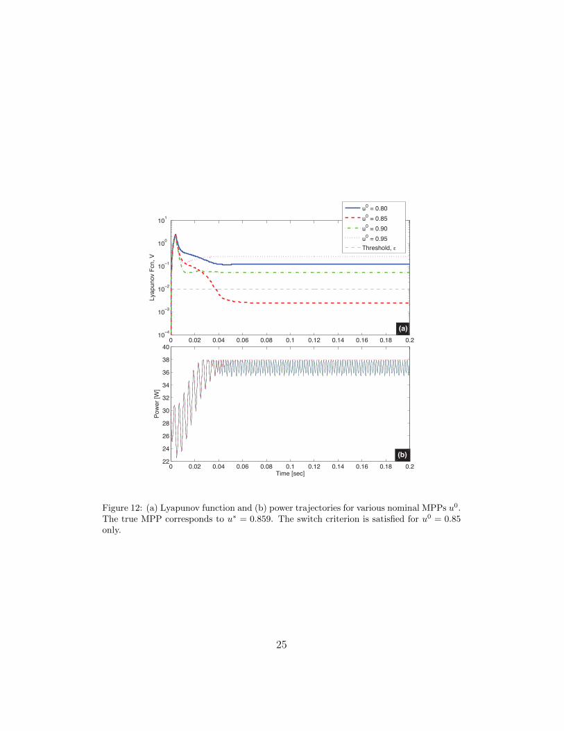
Next we examine the impact of large errors between the nominal u0 andoptimal u∗ MPPs. Recall that the Lyapunov function calculated in (28)measures the system’s proximity to u0, measured in the coordinate systemdefined by (5)-(6). If |u0−u∗| is sufficiently large, then the switching criterionV (xa) ≤ ε may never be satisfied and the perturbation amplitude will notdecay. Figure 12 demonstrates the Lyapunov function and power trajectoriesfor various values of u0. In all cases except one (u0 = 0.85) the switchingcriterion is not satisfied and the power oscillates around the true MPP. Underthis worst-case scenario Lyap-ES degenerates into basic ES.

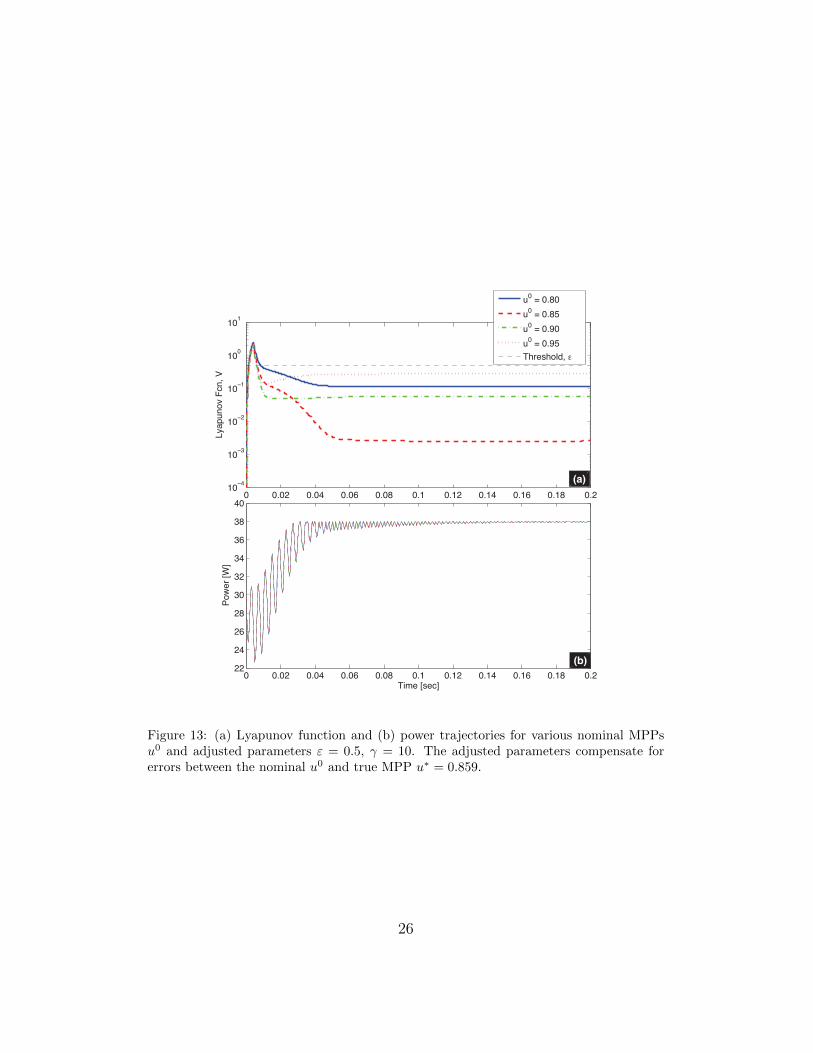
Degeneration of Lyap-ES into ES can be mitigated by appropriately se-lecting the threshold parameter ε and amplitude decay gain γ. That is, onemay select ε sufficiently large and γ sufficiently small such that the algo-rithm enters the exponential decay mode quickly and the perturbation de-cays slowly. Figure 13 provides an example, where the threshold was raisedto ε = 0.5 and the decay rate was lowered to γ = 10. Observe that theswitching criterion is satisfied in all cases. Consequently, Lyap-ES convergesand decays to the true MPP.

4. Conclusion

In this paper we propose a novel Lyapunov-based switched extremumseeking control method (Lyap-ES) that provides a practical extension toexisting research on ES by eliminating limit cycles. Lyap-ES guaranteesasymptotic convergence to the extremum of a static map by exponentially

21

decaying the perturbation once the algorithm reaches a neighborhood of theextremum. This neighborhood is approximated via Lyapunov stability anal-ysis concepts that extend the stability proof originally presented in [13]. Weapply Lyap-ES to the MPPT problem in a PV system as a case study toanalyze performance. The advantage of Lyap-ES over traditional MPPTmethods, e.g. P&O, is that the algorithm converges to the MPP asymptoti-cally without entering a limit cycle. Moreover, the method is self-optimizingwith respect to disturbances, such as varying solar irradiation and temper-ature shifts. We study Lyap-ES for MPPT in two steps. First, the conceptis demonstrated by applying step changes in environmental conditions. Sec-ond, experimentally measured light and temperature data is applied to studyLyap-ES under realistic operating conditions. Future work will involve im-plementation into experimental photovoltaic systems. In summary, Lyap-ESoffers a control-theoretic alternative for MPPT problems.

Appendix A. ES Control Parameter Selection

The synthesis process for an extremum seeking controller requires properselection of the perturbation frequency ω, amplitude a0, gradient update lawgain k, and filter cut-off frequencies ωh and ωl. The perturbation frequencymust be slower than the slowest plant dynamics to ensure the plant appearsas a static nonlinearity from the viewpoint of the ES feedback loop. Math-ematically, this can be enforced by ensuring ω mineig(A) , where Ais the state matrix from linearizing the plant. Large values for a0 and kallow faster convergence rates, but respectively increase oscillation ampli-tude and sensitivity to disturbances. More importantly, they can destroystability. Therefore, one typically increases these parameter values to ob-tain maximum convergence speed for a permissible amount of oscillation andsensitivity. The filter cut-off frequencies must be designed in coordinationwith the perturbation frequency ω. Specifically, the high-pass filter must notattenuate the perturbation frequency, but the low-pass filter should - thusbounding the cut-off frequencies from above. Mathematically ωh < ω andωl < ω. Moreover, the filters should have sufficiently fast dynamics to re-spond quickly to perturbations in the control input, thereby bounding thecut-off frequencies from below. Generally, proper selection of the ES param-eters is a tuning process [15]. However, the above guidelines are valuable foreffective calibration.

22

0 200 400 600 800 1000 1200 1400 1600 1800 2000400

600

800

Irra

dia

nce

[W

/m2]

0 200 400 600 800 1000 1200 1400 1600 1800 200020

30

40

50

Te

mp

. [d

eg

C]

0 200 400 600 800 1000 1200 1400 1600 1800 200010

20

30

Po

we

r [W

]

0 200 400 600 800 1000 1200 1400 1600 1800 20000.85

0.9

0.95

Du

ty R

atio

0 200 400 600 800 1000 1200 1400 1600 1800 200010

0

101

102

103

104

Lya

pu

no

v F

cn

, V

Time [sec]

Lyapunov Fcn

Switch Threshold

Power

MPP

Figure 10: Evolution of solar irradiation, temperature, PV output power, DC/DC con-verter duty ratio, and the Lyapunov function value under the Lyap-ES control scheme. Azoom-in of the power and duty ratio outputs circumscribed by the rectangles are providedin Figure 11.

23

1500 1550 1600 1650 1700 1750 1800

15

20

25

Po

we

r [W

]

Power

MPP

1500 1550 1600 1650 1700 1750 18000.86

0.87

0.88

0.89

Du

ty R

atio

1500 1550 1600 1650 1700 1750 1800

101

102

Lya

pu

no

v F

cn

, V

Time [sec]

Lyapunov Fcn

Switch Threshold

Figure 11: Zoom-in of PV output power, DC/DC converter duty ratio and Lyapunovfunction value from Fig. 10. The yellow and white shaded time-zones denote when theperturbation is decaying and re-enabled, respectively, as determined by the Lyapunovfunction/threshold crossing.

24

0 0.02 0.04 0.06 0.08 0.1 0.12 0.14 0.16 0.18 0.210

−4

10−3

10−2

10−1

100

101

Lyapunov Fcn, V

0 0.02 0.04 0.06 0.08 0.1 0.12 0.14 0.16 0.18 0.222

24

26

28

30

32

34

36

38

40

Power [W

]

Time [sec]

u0 = 0.80

u0 = 0.85

u0 = 0.90

u0 = 0.95

Threshold, ε

(a)

(b)

Figure 12: (a) Lyapunov function and (b) power trajectories for various nominal MPPs u0.The true MPP corresponds to u∗ = 0.859. The switch criterion is satisfied for u0 = 0.85only.

25

0 0.02 0.04 0.06 0.08 0.1 0.12 0.14 0.16 0.18 0.210

−4

10−3

10−2

10−1

100

101

Lyapunov Fcn, V

0 0.02 0.04 0.06 0.08 0.1 0.12 0.14 0.16 0.18 0.222

24

26

28

30

32

34

36

38

40

Power [W

]

Time [sec]

u0 = 0.80

u0 = 0.85

u0 = 0.90

u0 = 0.95

Threshold, ε

(a)

(b)

Figure 13: (a) Lyapunov function and (b) power trajectories for various nominal MPPsu0 and adjusted parameters ε = 0.5, γ = 10. The adjusted parameters compensate forerrors between the nominal u0 and true MPP u∗ = 0.859.

26

References

[1] T. Esram, P. Chapman, Comparison of photovoltaic array maximumpower point tracking techniques, IEEE Transactions on Energy Conver-sion 22 (2007) 439–449.

[2] J. Kwon, B. Kwon, K. Nam, Three-phase photovoltaic system withthree-level boosting MPPT control, IEEE Transactions on Power Elec-tronics 23 (2008) 2319–2327.

[3] N. Femia, G. Petrone, G. Spagnuolo, M. Vitelli, Optimization of perturband observe maximum power point tracking method, IEEE Transactionson Power Electronics 20 (2005) 963–973.

[4] V. T. Buyukdegirmenci, A. M. Bazzi, P. T. Krein, A comparative studyof an exponential adaptive perturb and observe algorithm and ripplecorrelation control for real-time optimization, 2010 IEEE Workshop onControl and Modeling for Power Electronics (2010).

[5] K. Hussein, I. Muta, T. Hoshino, M. Osakada, Maximum photovoltaicpower tracking: an algorithm for rapidly changing atmospheric condi-tions, IEE Proceedings-Generation, Transmission and Distribution 142(1995) 59–64.

[6] H. El Fadil, F. Giri, Climatic sensorless maximum power point trackingin pv generation systems, Control Engineering Practice 19 (2011) 513 –521.

[7] R. Leyva, C. Alonso, I. Queinnec, A. Cid-Pastor, D. Lagrange,L. Martinez-Salamero, Mppt of photovoltaic systems using extremum -seeking control, IEEE Transactions on Aerospace and Electronic Sys-tems 42 (2006) 249 – 258.

[8] A. Bratcu, I. Munteanu, S. Bacha, B. Raison, Maximum power pointtracking of grid-connected photovoltaic arrays by using extremum seek-ing control, Journal of Control Engineering and Applied Informatics 10(2008) 3–12.

[9] T. Esram, J. W. Kimball, P. T. Krein, P. L. Chapman, P. Midya, Dy-namic maximum power point tracking of photovoltaic arrays using ripple

27

correlation control, IEEE Transactions on Power Electronics 21 (2006)1282 – 1290.

[10] D. Logue, P. Krein, Optimization of power electronic systems usingripple correlation control: A dynamic programming approach, PESCRecord - IEEE Annual Power Electronics Specialists Conference 2 (2001)459 – 464.

[11] S. L. Brunton, C. W. Rowley, S. R. Kulkarni, C. Clarkson, Maximumpower point tracking for photovoltaic optimization using ripple-basedextremum seeking control, IEEE Transactions on Power Electronics 25(2010) 2531 – 2540.

[12] A. M. Bazzi, P. T. Krein, Concerning maximum power point tracking forphotovoltaic optimization using ripple-based extremum seeking control,IEEE Transactions on Power Electronics 26 (2011) 1611 – 1612.

[13] M. Krstic, H. Wang, Stability of extremum seeking feedback for generalnonlinear dynamic systems, Automatica 36 (2000) 595–601.

[14] D. DeHaan, M. Guay, Extremum-seeking control of state-constrainednonlinear systems, Automatica 41 (2005) 1567–1574.

[15] Y. Chang, S. Moura, Air flow control in fuel cell systems: An extremumseeking approach, Proceedings of the 2009 American Control Conference(2009) 1052–1059.

[16] J. Creaby, Y. Li, S. Seem, Maximizing Wind Energy Capture via Ex-tremum Seeking Control, Proceedings of the 2008 ASME Dynamic Sys-tems and Control Conference (2008) 361–387.

[17] K. Ariyur, M. Krstic, Real-time optimization by extremum-seeking con-trol, Wiley-Blackwell, 2003.

[18] M. Krstic, Performance improvement and limitations in extremum seek-ing control, Systems & Control Letters 39 (2000) 313–326.

[19] Y. Tan, D. Nesic, I. Mareels, On the choice of dither in extremumseeking systems: A case study, Automatica 44 (2008) 1446–1450.

28

[20] D. Nesic, Y. Tan, W. Moase, C. Manzie, A unifying approach to ex-tremum seeking: Adaptive schemes based on estimation of derivatives,Proceedings of the IEEE Conference on Decision and Control (2010)4625–4630.

[21] S. Moura, Y. Chang, Asymptotic convergence through lyapunov-basedswitching in extremum seeking with application to photovoltaic systems,Proceedings of the 2010 American Control Conference (2010) 3542–3548.

[22] A. Ghaffari, M. Krstic, D. Nesic, Multivariable Newton-based extremumseeking, Proceedings of the IEEE Conference on Decision and Control(2011) 4436–4441.

[23] H. Khalil, Nonlinear systems, volume 3, Prentice hall, 1992.

[24] S. Bull, Renewable energy today and tomorrow, Proceedings of theIEEE 89 (2001) 1216 –1226.

[25] G. Vachtsevanos, K. Kalaitzakis, A hybrid photovoltaic simulator forutility interactive studies, IEEE Transactions on Energy Conversion(1987) 227–231.

[26] G. Masters, Renewable and efficient electric power systems, Wiley On-line Library, 2004.

[27] D. Chan, J. Phang, Analytical methods for the extraction of solar-cell single-and double-diode model parameters from iv characteristics, ,IEEE Transactions on Electron Devices 34 (1987) 286–293.

[28] J. Gow, C. Manning, Development of a photovoltaic array model for usein power-electronics simulation studies, in: IEE Proceedings-ElectricPower Applications, volume 146, IET, pp. 193–200.

[29] M. Villalva, J. Gazoli, et al., Comprehensive approach to modeling andsimulation of photovoltaic arrays, Power Electronics, IEEE Transactionson 24 (2009) 1198–1208.

[30] S. R. Sanders, J. Noworolski, X. Z. Liu, G. C. Verghese, Generalizedaveraging method for power conversion circuits, IEEE Transactions onPower Electronics 6 (1991) 251 – 259.

29