Lucas-Kanade 20 Years On: A Unifying Framework Part 1: The ... · Lucas-Kanade 20 Years On: A...

To Appear in the International Journal of Computer Vision

Lucas-Kanade 20 Years On: A Unifying Framework

Part 1: The Quantity Approximated, the Warp Update Rule,and the Gradient Descent Approximation

Simon Baker and Iain Matthews

The Robotics InstituteCarnegie Mellon University

Pittsburgh, PA 15213

Abstract

Since the Lucas-Kanade algorithm was proposed in 1981 image alignment has be-come one of the most widely used techniques in computer vision. Applications rangefrom optical flow and tracking to layered motion, mosaic construction, and face cod-ing. Numerous algorithms have been proposed and a wide variety of extensions havebeen made to the original formulation. We present an overview of image alignment,describing most of the algorithms and their extensions in a consistent framework. Weconcentrate on the inverse compositional algorithm, an efficient algorithm that we re-cently proposed. We examine which of the extensions to Lucas-Kanade can be usedwith the inverse compositional algorithm without any significant loss of efficiency, andwhich cannot. In this paper, Part 1 in a series of papers, we cover the quantity approxi-mated, the warp update rule, and the gradient descent approximation. In future paperswe will cover the choice of the norm, how to allow linear appearance variation, howto impose priors on the parameters, and various techniques to avoid local minima.

Keywords: Image alignment, Lucas-Kanade, a unifying framework, additive vs. com-positional algorithms, forwards vs. inverse algorithms, the inverse compositional al-gorithm, efficiency, steepest descent, Gauss-Newton, Newton, Levenberg-Marquardt.

1 Introduction

Image alignment consists of moving, and possibly deforming, a template to minimize the differ-

ence between the template and an image. Since the first use of image alignment in the Lucas-

Kanade optical flow algorithm [13], image alignment has become one of the most widely used

techniques in computer vision. Besides optical flow, some of its other applications include track-

ing [5, 12], parametric and layered motion estimation [4], mosaic construction [16], medical image

registration [7], and face coding [2, 8].

The usual approach to image alignment is gradient descent. A variety of other numerical al-

gorithms such as difference decomposition [11] and linear regression [8] have also been proposed,

but gradient descent is the defacto standard. Gradient descent can be performed in variety of dif-

ferent ways, however. One difference between the various approaches is whether they estimate

an additive increment to the parameters (the additive approach [13]), or whether they estimate an

incremental warp that is then composed with the current estimate of the warp (the compositional

approach [16].) Another difference is whether the algorithm performs a Gauss-Newton, a Newton,

a steepest-descent, or a Levenberg-Marquardt approximation in each gradient descent step.

We propose a unifying framework for image alignment, describing the various algorithms and

their extensions in a consistent manner. Throughout the framework we concentrate on the inverse

compositional algorithm, an efficient algorithm that we recently proposed [2]. We examine which

of the extensions to Lucas-Kanade can be applied to the inverse compositional algorithm without

any significant loss of efficiency, and which extensions require additional computation. Wherever

possible we provide empirical results to illustrate the various algorithms and their extensions.

In this paper, Part 1 in a series of papers, we begin in Section 2 by reviewing the Lucas-Kanade

algorithm. We proceed in Section 3 to analyze the quantity that is approximated by the various

image alignment algorithms and the warp update rule that is used. We categorize algorithms as

either additive or compositional, and as either forwards or inverse. We prove the first order equiv-

alence of the various alternatives, derive the efficiency of the resulting algorithms, describe the set

of warps that each alternative can be applied to, and finally empirically compare the algorithms.

In Section 4 we describe the various gradient descent approximations that can be used in each

iteration, Gauss-Newton, Newton, diagonal Hessian, Levenberg-Marquardt, and steepest-descent

[14]. We compare these alternatives both in terms of speed and in terms of empirical performance.

We conclude in Section 5 with a discussion. In future papers in this series (currently under prepa-

ration), we will cover the choice of the error norm, how to allow linear appearance variation, how

to add priors on the parameters, and various techniques to avoid local minima.

1

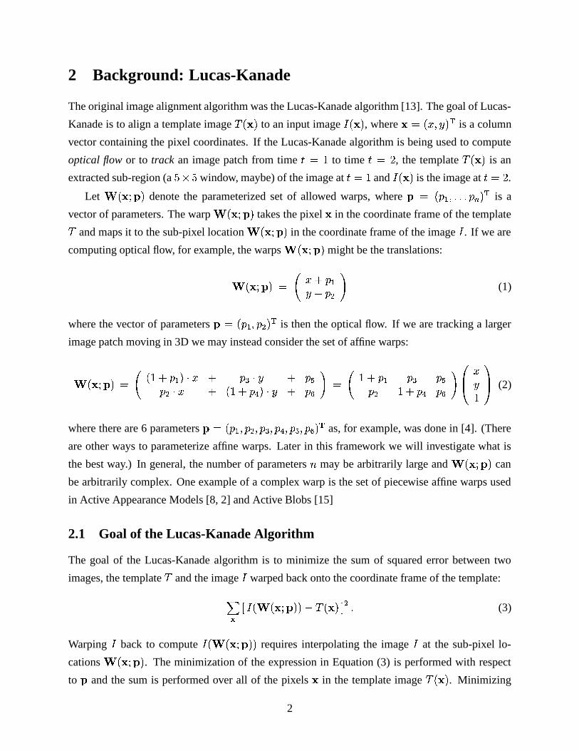
2 Background: Lucas-Kanade

The original image alignment algorithm was the Lucas-Kanade algorithm [13]. The goal of Lucas-

Kanade is to align a template image��

to an input image � �� , where��

is a column

vector containing the pixel coordinates. If the Lucas-Kanade algorithm is being used to compute

optical flow or to track an image patch from time � ��to time � ��

, the template��

is an

extracted sub-region (a �� window, maybe) of the image at � ��and � �� is the image at � ��

.

Let �!�#"%$&�denote the parameterized set of allowed warps, where

$' �)(+*,�.-.-/- (102� �is a

vector of parameters. The warp �!�#"%$&�takes the pixel

�in the coordinate frame of the template�

and maps it to the sub-pixel location ��#"%$&�in the coordinate frame of the image � . If we are

computing optical flow, for example, the warps ��3"%$4�might be the translations:

�!�#"%$&�5 6 �879(:*�;7<(�=?> (1)

where the vector of parameters$@A�B(C*D�E(�=/�F�

is then the optical flow. If we are tracking a larger

image patch moving in 3D we may instead consider the set of affine warps:

�!�#"%$&�? 6 �G�47<(H*D�JIK� 7 (�L4IK� 7 (�M(�=NI/� 7 �G�N79(1O,�JIK� 7 (�P > 6 �Q7<(H* (�L (1M(�= �N7<(1O�(1P >�RST � � �VUXWY (2)

where there are 6 parameters$Z[�)(C*/�E(1=.�E(�L.� (1OK�E(�M/�E(�P,�E�

as, for example, was done in [4]. (There

are other ways to parameterize affine warps. Later in this framework we will investigate what is

the best way.) In general, the number of parameters \ may be arbitrarily large and �!�#"%$&�can

be arbitrarily complex. One example of a complex warp is the set of piecewise affine warps used

in Active Appearance Models [8, 2] and Active Blobs [15]

2.1 Goal of the Lucas-Kanade Algorithm

The goal of the Lucas-Kanade algorithm is to minimize the sum of squared error between two

images, the template�

and the image � warped back onto the coordinate frame of the template:]�^`_ � � ��#"%$&�%�Ja�8�!��2b = -(3)

Warping � back to compute � � ��#"G$4�G�requires interpolating the image � at the sub-pixel lo-

cations �!�#"%$&�. The minimization of the expression in Equation (3) is performed with respect

to$

and the sum is performed over all of the pixels�

in the template image��

. Minimizing

2

the expression in Equation (1) is a non-linear optimization task even if �!�#"%$&�is linear in

$because the pixel values � �� are, in general, non-linear in

�. In fact, the pixel values � �� are

essentially un-related to the pixel coordinates�

. To optimize the expression in Equation (3), the

Lucas-Kanade algorithm assumes that a current estimate of$

is known and then iteratively solves

for increments to the parameters � $ ; i.e. the following expression is (approximately) minimized:] ^ _ � � ��#"%$ 7 � $4�G�Ja ��2b = (4)

with respect to � $ , and then the parameters are updated:$�� $V7 � $N- (5)

These two steps are iterated until the estimates of the parameters$

converge. Typically the test for

convergence is whether some norm of the vector � $ is below a threshold � ; i.e. �� $ �� .2.2 Derivation of the Lucas-Kanade Algorithm

The Lucas-Kanade algorithm (which is a Gauss-Newton gradient descent non-linear optimization

algorithm) is then derived as follows. The non-linear expression in Equation (4) is linearized by

performing a first order Taylor expansion on � � ��#"G$ 7 � $&�%� to give:]X^ � � ��3"%$4�G� 7�� $ � $9a �� = - (6)

In this expression,� � �� is the gradient of image � evaluated at ��3"%$4�

; i.e.� � is

computed in the coordinate frame of � and then warped back onto the coordinate frame of�

using the current estimate of the warp �!�#"%$&�. The term

�� is the Jacobian of the warp. If �!�#"%$&�� !�#"%$&� �� #"%$&�%�E� then:

� � $ RT �� "! ��#�%$ -/-.- ��&��#��'��&(� � ! ��(�#� $ -/-.- ��&(�#� ' UY - (7)

We follow the notational convention that the partial derivatives with respect to a column vector are

laid out as a row vector. This convention has the advantage that the chain rule results in a matrix

multiplication, as in the expression in Equation (6). For example, the affine warp in Equation (2)

has the Jacobian:

� � $ 6 � ) � ) � )) � ) � ) � > - (8)

3

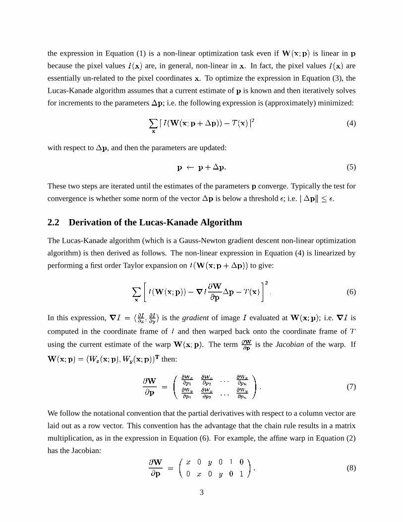
The Lucas-Kanade Algorithm

Iterate:

(1) Warp � with �� to compute �� (2) Compute the error image ��(3) Warp the gradient �� with �!�#"%$&�(4) Evaluate the Jacobian

�� at ��(5) Compute the steepest descent images �� (6) Compute the Hessian matrix using Equation (11)(7) Compute �

^��

(8) Compute �� using Equation (10)(9) Update the parameters �! "�$#%�&�

until '(�&�)'+*-,Figure 1: The Lucas-Kanade algorithm [13] consists of iteratively applying Equations (10) & (5) until theestimates of the parameters � converge. Typically the test for convergence is whether some norm of thevector �&� is below a user specified threshold , . Because the gradient �� must be evaluated at ��and the Jacobian

�� must be evaluated at � , all 9 steps must be repeated in every iteration of the algorithm.

Minimizing the expression in Equation (6) is a least squares problem and has a closed from solution

which can be derived as follows. The partial derivative of the expression in Equation (6) with

respect to � $ is: � ] ^ � � � � $ � � � � �!�#"%$&�%� 7 � � � � $ � $9a ��!�� (9)

where we refer to� � �� as the steepest descent images. (See Section 4.3 for why.) Setting

this expression to equal zero and solving gives the closed form solution for the minimum of the

expression in Equation (6) as:

� $� .-/ * ] ^ � � � � $ � � _ �� a � � �!�#"%$&�%�Eb(10)

where.

is the \9� \ (Gauss-Newton approximation to the) Hessian matrix:

. ]�^ � � � � $ � � � � � � $ ��-(11)

For reasons that will become clear later we refer to �^ _ � � �� b � _ �� a � � ��#"%$&�%�Eb

as the steep-

est descent parameter updates. Equation (10) then expresses the fact that the parameter updates� $ are the steepest descent parameter updates multiplied by the inverse of the Hessian matrix.

The Lucas-Kanade algorithm [13] then consists of iteratively applying Equations (10) and (5). See

4

1 2 3 4 5 6−0.5

0

0.5

1

1.5

1 2 3 4 5 6−0.06

−0.04

−0.02

0

0.02

1 2 3 4 5 6−3

−2

−1

0

1

2

3

4x 10

7

Inverse Hessian

Hessian

Template

Warped

Error

Image Gradient YImage Gradient X

SD Parameter Updates

Warp Parameters

Parameter Updates

Warped Gradients Jacobian

Steepest Descent Images

Image

Step 4

Step 6

Step 8

Ste

p 2

Step 7

Step 3

Step 9

Step 7

Step 1

Step 5

�

� �

��

��

��

��

��

��

��

�

��

-

+

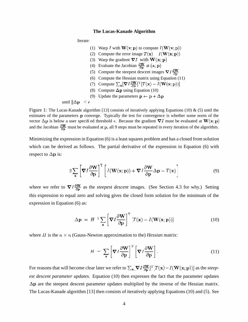
!�"�# �� $&% ' # �� (� �� )� � �*� %Figure 2: A schematic overview of the Lucas-Kanade algorithm [13]. The image � is warped with thecurrent estimate of the warp in Step 1 and the result subtracted from the template in Step 2 to yield the errorimage. The gradient of � is warped in Step 3, the Jacobian is computed in Step 4, and the two combinedin Step 5 to give the steepest descent images. In Step 6 the Hessian is computed from the steepest descentimages. In Step 7 the steepest descent parameter updates are computed by dot producting the error imagewith the steepest descent images. In Step 8 the Hessian is inverted and multiplied by the steepest descentparameter updates to get the final parameter updates �&� which are then added to the parameters � in Step 9.

Figures 1 and 2 for a summary. Because the gradient� � must be evaluated at �!�#"%$&�

and the

Jacobian�� at

$, they both in general depend on

$. For some simple warps such as the transla-

tions in Equation (1) and the affine warps in Equation (2) the Jacobian can sometimes be constant.

See for example Equation (8). In general, however, all 9 steps of the algorithm must be repeated

in every iteration because the estimates of the parameters$

vary from iteration to iteration.

5

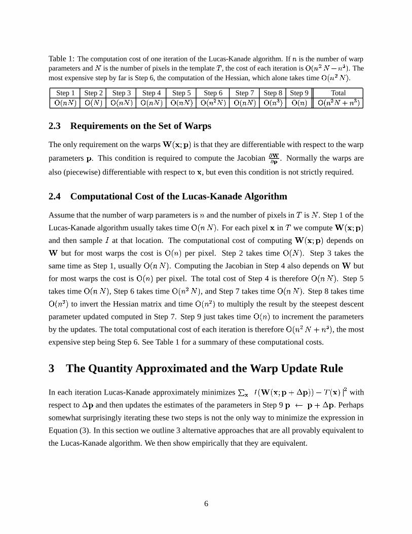
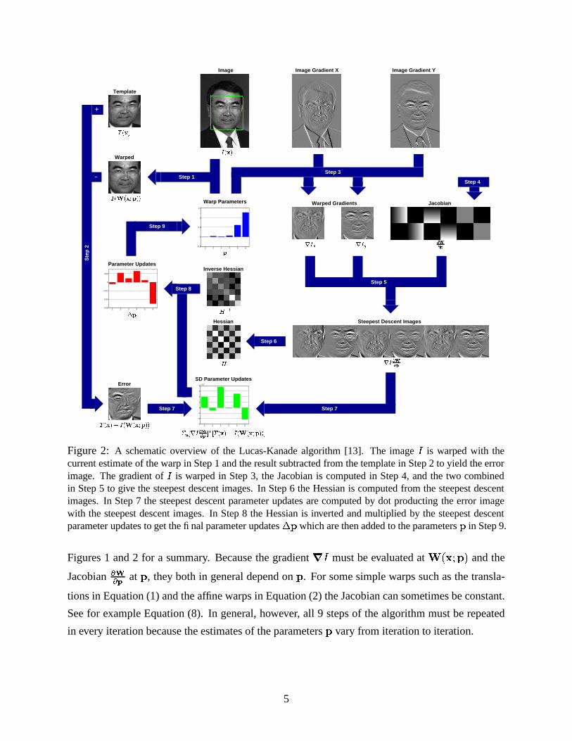
Table 1: The computation cost of one iteration of the Lucas-Kanade algorithm. If � is the number of warpparameters and

�is the number of pixels in the template � , the cost of each iteration is � �� = � #�� L . The

most expensive step by far is Step 6, the computation of the Hessian, which alone takes time � �� = � .Step 1 Step 2 Step 3 Step 4 Step 5 Step 6 Step 7 Step 8 Step 9 Total�&�� = � � �� L � �� = � #�� L

2.3 Requirements on the Set of Warps

The only requirement on the warps �!�#"%$&�is that they are differentiable with respect to the warp

parameters$

. This condition is required to compute the Jacobian�� . Normally the warps are

also (piecewise) differentiable with respect to�

, but even this condition is not strictly required.

2.4 Computational Cost of the Lucas-Kanade Algorithm

Assume that the number of warp parameters is \ and the number of pixels in�

is � . Step 1 of the

Lucas-Kanade algorithm usually takes time � � \�� . For each pixel�

in�

we compute �!�#"%$&�and then sample � at that location. The computational cost of computing �!�#"%$&�

depends on but for most warps the cost is � � \ � per pixel. Step 2 takes time � � � � . Step 3 takes the

same time as Step 1, usually � � \�� . Computing the Jacobian in Step 4 also depends on but

for most warps the cost is � � \ � per pixel. The total cost of Step 4 is therefore � � \�� . Step 5

takes time � � \�� , Step 6 takes time � � \ = � � , and Step 7 takes time � � \�� . Step 8 takes time

� � \ L � to invert the Hessian matrix and time � � \ = � to multiply the result by the steepest descent

parameter updated computed in Step 7. Step 9 just takes time � � \ � to increment the parameters

by the updates. The total computational cost of each iteration is therefore � � \ = � 7 \ L � , the most

expensive step being Step 6. See Table 1 for a summary of these computational costs.

3 The Quantity Approximated and the Warp Update Rule

In each iteration Lucas-Kanade approximately minimizes �^ _ � � ��#"G$V7 � $&�%�Ja ��2b = with

respect to � $ and then updates the estimates of the parameters in Step 9$ � $57 � $Q- Perhaps

somewhat surprisingly iterating these two steps is not the only way to minimize the expression in

Equation (3). In this section we outline 3 alternative approaches that are all provably equivalent to

the Lucas-Kanade algorithm. We then show empirically that they are equivalent.

6

3.1 Compositional Image Alignment

The first alternative to the Lucas-Kanade algorithm is the compositional algorithm.

3.1.1 Goal of the Compositional Algorithm

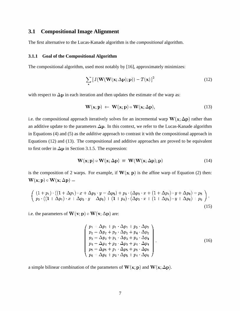
The compositional algorithm, used most notably by [16], approximately minimizes:] ^ _ � � � ��3" � $4��"%$4�G� a ��2b = (12)

with respect to � $ in each iteration and then updates the estimate of the warp as: ��#"%$&� � ��3"%$4�� #" � $&� � (13)

i.e. the compositional approach iteratively solves for an incremental warp �!�#" � $4� rather than

an additive update to the parameters � $ . In this context, we refer to the Lucas-Kanade algorithm

in Equations (4) and (5) as the additive approach to contrast it with the compositional approach in

Equations (12) and (13). The compositional and additive approaches are proved to be equivalent

to first order in � $ in Section 3.1.5. The expression: ��#"G$4�� !�#" � $4�� #" � $&� "%$&� (14)

is the composition of 2 warps. For example, if �!�#"%$&�is the affine warp of Equation (2) then: �!�#"%$&�� 3" � $4�36 �G�47<(H*D�JI2�%��47 � (H*D�JIK� 7 � (�L&IK� 7 � (�M,�C7<(�L4I2� � (�=&IK� 7 �G�N7 � (1O/�JIK�;7 � (�P,�C7<(�M(�=&I2�%��Q7 � (H* �JIK� 7 � (�LNI/� 7 � (�M,�+7 �G�479( O.�JI2� � (�=&IK� 7 �G�N7 � (1O/�JIK�;7 � (�P,�C7<(�P > �

(15)

i.e. the parameters of ��3"%$4�� !�#" � $&� are:

RSSSSSSSST(H* 7 � (:*�7<(H*&I � (H* 7<(�LNI � (�=(�=�7 � (1=37<(�=NI � (H* 7<(1OQI � (�=(�L�7 � (1L37<(H*&I � (�L�7<(�LNI � (1O(1O�7 � ( O#7<(�=NI � (�L�7<(1OQI � (1O(�M�7 � (1M37<(H*&I � (�M�7<(�LNI � (�P(�P�7 � (1P37<(�=NI � (�M�7<(1OQI � (�P

UXWWWWWWWWY�

(16)

a simple bilinear combination of the parameters of ��3"%$4�and ��#" � $&� .

7

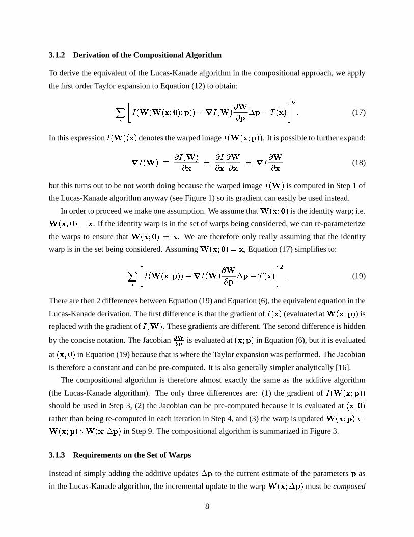
3.1.2 Derivation of the Compositional Algorithm

To derive the equivalent of the Lucas-Kanade algorithm in the compositional approach, we apply

the first order Taylor expansion to Equation (12) to obtain:] ^ � � � �!�#"��C� "G$4�G�H7 � � � � � � $ � $9a�8�!�� = - (17)

In this expression � � � ��denotes the warped image � � ��#"%$&�%�

. It is possible to further expand:

� � � � � � � � �� (18)

but this turns out to be not worth doing because the warped image � � �is computed in Step 1 of

the Lucas-Kanade algorithm anyway (see Figure 1) so its gradient can easily be used instead.

In order to proceed we make one assumption. We assume that ��#"��+�is the identity warp; i.e. �!�#"��C�3 �

. If the identity warp is in the set of warps being considered, we can re-parameterize

the warps to ensure that �!�#"��C�8'�. We are therefore only really assuming that the identity

warp is in the set being considered. Assuming ��#"��C�� , Equation (17) simplifies to:] ^ � � �!�#"%$&�%� 7 � � � � � � $ � $<a �� = - (19)

There are then 2 differences between Equation (19) and Equation (6), the equivalent equation in the

Lucas-Kanade derivation. The first difference is that the gradient of � �!�� (evaluated at ��#"G$4�) is

replaced with the gradient of � � �. These gradients are different. The second difference is hidden

by the concise notation. The Jacobian�� is evaluated at

��#"%$&�in Equation (6), but it is evaluated

at�!�#"��C�

in Equation (19) because that is where the Taylor expansion was performed. The Jacobian

is therefore a constant and can be pre-computed. It is also generally simpler analytically [16].

The compositional algorithm is therefore almost exactly the same as the additive algorithm

(the Lucas-Kanade algorithm). The only three differences are: (1) the gradient of � � ��3"%$4�G�should be used in Step 3, (2) the Jacobian can be pre-computed because it is evaluated at

�!�#"��C�rather than being re-computed in each iteration in Step 4, and (3) the warp is updated �!�#"%$&� � �!�#"%$&�� 3" � $4� in Step 9. The compositional algorithm is summarized in Figure 3.

3.1.3 Requirements on the Set of Warps

Instead of simply adding the additive updates � $ to the current estimate of the parameters$

as

in the Lucas-Kanade algorithm, the incremental update to the warp ��#" � $&� must be composed

8

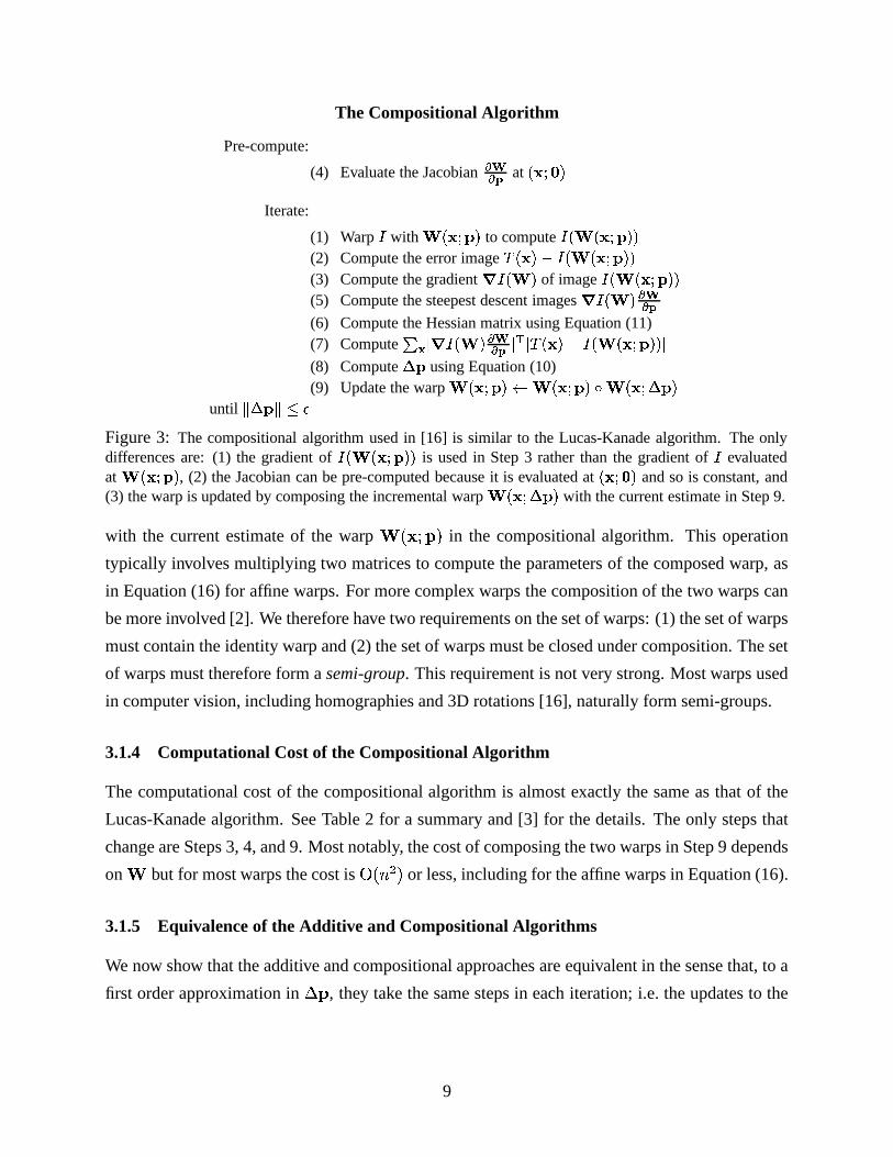
The Compositional Algorithm

Pre-compute:

(4) Evaluate the Jacobian�� at ��

Iterate:

(1) Warp � with �� to compute �� (2) Compute the error image ��(3) Compute the gradient �!�� of image �� (5) Compute the steepest descent images �� (6) Compute the Hessian matrix using Equation (11)(7) Compute �

^��

(8) Compute �� using Equation (10)(9) Update the warp �� &��

until '(�&�)'+*-,Figure 3: The compositional algorithm used in [16] is similar to the Lucas-Kanade algorithm. The onlydifferences are: (1) the gradient of �� is used in Step 3 rather than the gradient of � evaluatedat �� , (2) the Jacobian can be pre-computed because it is evaluated at �� and so is constant, and(3) the warp is updated by composing the incremental warp �� &� with the current estimate in Step 9.

with the current estimate of the warp ��#"%$&�in the compositional algorithm. This operation

typically involves multiplying two matrices to compute the parameters of the composed warp, as

in Equation (16) for affine warps. For more complex warps the composition of the two warps can

be more involved [2]. We therefore have two requirements on the set of warps: (1) the set of warps

must contain the identity warp and (2) the set of warps must be closed under composition. The set

of warps must therefore form a semi-group. This requirement is not very strong. Most warps used

in computer vision, including homographies and 3D rotations [16], naturally form semi-groups.

3.1.4 Computational Cost of the Compositional Algorithm

The computational cost of the compositional algorithm is almost exactly the same as that of the

Lucas-Kanade algorithm. See Table 2 for a summary and [3] for the details. The only steps that

change are Steps 3, 4, and 9. Most notably, the cost of composing the two warps in Step 9 depends

on but for most warps the cost is � � \ = � or less, including for the affine warps in Equation (16).

3.1.5 Equivalence of the Additive and Compositional Algorithms

We now show that the additive and compositional approaches are equivalent in the sense that, to a

first order approximation in � $ , they take the same steps in each iteration; i.e. the updates to the

9

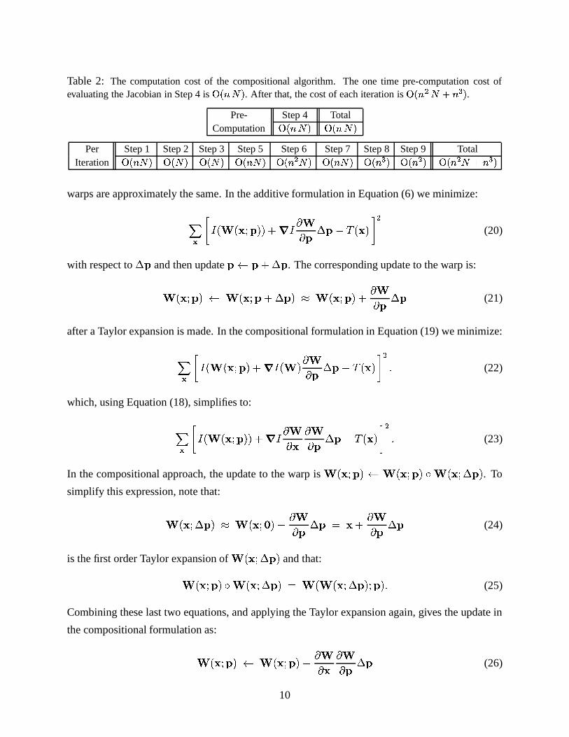
Table 2: The computation cost of the compositional algorithm. The one time pre-computation cost ofevaluating the Jacobian in Step 4 is � �� . After that, the cost of each iteration is �&�� = � #�� L .

Pre- Step 4 TotalComputation �&��

Per Step 1 Step 2 Step 3 Step 5 Step 6 Step 7 Step 8 Step 9 TotalIteration � �� &� � � � � � �� = � � �� &�� L � �� = � �� = � # � L

warps are approximately the same. In the additive formulation in Equation (6) we minimize:] ^ � � ��#"%$&�%�H7 � � � � $ � $9a �� = (20)

with respect to � $ and then update$ � $V7 � $ . The corresponding update to the warp is:

��#"G$4� � �!�#"%$V7 � $&�� !�#"%$&� 7 � � $ � $ (21)

after a Taylor expansion is made. In the compositional formulation in Equation (19) we minimize:] ^ � � �!�#"%$&� 7 � � � � � � $ � $ a �8�!�� = - (22)

which, using Equation (18), simplifies to:] ^ � � �!�#"%$&�%� 7 � � � � � � � $ � $9a �� = - (23)

In the compositional approach, the update to the warp is �!�#"%$&� � ��#"%$&� � ��3" � $4� . To

simplify this expression, note that:

�!�#" � $&�� 3"��C� 7 � � $ � $� � 7 � � $ � $ (24)

is the first order Taylor expansion of �!�#" � $4� and that: �!�#"%$&�� #" � $&�5 � �!�#" � $&� "%$&� - (25)

Combining these last two equations, and applying the Taylor expansion again, gives the update in

the compositional formulation as:

��#"G$4� � �!�#"%$&�C7 � � � � � $ � $ (26)

10

to first order in � $ . The difference between the additive formulation in Equations (20) and (21),

and the compositional formulation in Equations (23) and (26) is that�� is replaced by

�� ^ �� .

Equations (20) and (22) therefore generally result in different estimates for � $ . (Note that in the

second of these expressions�� is evaluated at

�!�#"��C�, rather than at

��3"%$4�in the first expression.)

If the vectors�� in the additive formulation and

�� ^ �� in the compositional formulation both

span the same linear space, however, the final updates to the warp in Equations (21) and (26) will

be the same to first order in � $ and the two formulations are equivalent to first order in � $ ; i.e. the

optimal value of�� $ in Equation (20) will approximately equal the optimal value of

�� ^ �� $in Equation (22). From Equation (21) we see that the first of these expressions:

� � $ � ��#"%$ 7 � $4�� $ (27)

and from Equation (26) we see that the second of these expressions:

� � � � � $ � �!�#"%$&� � �!�#"%$ 7 � $4�� $ -

(28)

The vectors�� in the additive formulation and

�� ^ �� in the compositional formulation therefore

span the same linear space, the tangent space of the manifold ��#"G$4�, if (there is an �� )

such

that) for any � $ ( �� $ �� ) there is a � $�� such that: �!�#"%$V7 � $&� ��#"%$&�� 3"%$ 7 � $ � ��- (29)

This condition means that the function between � $ and � $ � is defined in both directions. The

expressions in Equations (27) and (28) therefore span the same linear space. If the warp is invertible

Equation (29) always holds since � $�� can be chosen such that: ��#"%$ 7 � $ � � �!�#"%$&� / * � ��3"%$V7 � $&� - (30)

In summary, if the warps are invertible then the two formulations are equivalent. In Section 3.1.3,

above, we stated that the set of warps must form a semi-group for the compositional algorithm to

be applied. While this is true, for the compositional algorithm also to be provably equivalent to the

Lucas-Kanade algorithm, the set of warps must form a group; i.e. every warp must be invertible.

3.2 Inverse Compositional Image Alignment

As a number of authors have pointed out, there is a huge computational cost in re-evaluating the

Hessian in every iteration of the Lucas-Kanade algorithm [12, 9, 16]. If the Hessian were constant

11

it could be precomputed and then re-used. Each iteration of the algorithm (see Figure 1) would

then just consist of an image warp (Step 1), an image difference (Step 2), a collection of image

“dot-products” (Step 7), multiplication of the result by the Hessian (Step 8), and the update to the

parameters (Step 9). All of these operations can be performed at (close to) frame-rate [9].

Unfortunately the Hessian is a function of$

in both formulations. Although various approxi-

mate solutions can be used (such as only updating the Hessian every few iterations and approxi-

mating the Hessian by assuming it is approximately constant across the image [16]) these approx-

imations are inelegant and it is often hard to say how good approximations they are. It would be

far better if the problem could be reformulated in an equivalent way, but with a constant Hessian.

3.2.1 Goal of the Inverse Compositional Algorithm

The key to efficiency is switching the role of the image and the template, as in [12], where a change

of variables is made to switch or invert the roles of the template and the image. Such a change

of variables can be performed in either the additive [12] or the compositional approach [2]. (A

restricted version of the inverse compositional algorithm was proposed for homographies in [9].

Also, something equivalent to the inverse compositional algorithm may have been used in [11]. It

is hard to tell. The “difference decomposition” algorithm in [6] uses the additive approach how-

ever.) We first describe the inverse compositional approach because it is simpler. To distinguish

the previous algorithms from the new ones, we will refer to the original algorithms as the forwards

additive (i.e. Lucas-Kanade) and the forwards compositional algorithm. The corresponding algo-

rithms after the inversion will be called the inverse additive and inverse compositional algorithms.

The proof of equivalence between the forwards compositional and inverse compositional algo-

rithms is in Section 3.2.5. The result is that the inverse compositional algorithm minimizes:]X^ _ �8� �!�#" � $4�G� a � � ��#"%$&�%�2b =(31)

with respect to � $ (note that the roles of � and�

are reversed) and then updates the warp: ��3"%$4� � �!�#"%$&�� 3" � $4� / * - (32)

The only difference from the update in the forwards compositional algorithm in Equation (13) is

that the incremental warp �!�#" � $&� is inverted before it is composed with the current estimate.

12

For example, the parameters of the inverse of the affine warp in Equation (2) are:

��479(H*D�JI2��Q7<(1O/�Ja (�=&I�(�L RSSSSSSSSTa&(H*#a (H*3I�(1O379(�=&I�(�La&(�=a&(�La&(1ONa (H*3I�(1O379(�=&I�(�La&(�M4a (1O4I�(�M�79(�L&I�(�Pa&(�P4a (H*3I�(�P�79(�=&I�(�M

UXWWWWWWWWY-

(33)

If��7Z(H* �4I:��7Z(1O/�4a (1= I.(1L )

, the affine warp is degenerate and not invertible. All pixels

are mapped onto a straight line in � . We exclude all such affine warps from consideration. The

set of all such affine warps is then still closed under composition, as can be seen by computing�G�#7 (H*D�+I �G�37 ( O/��a (�=#IX(�Lfor the parameters in Equation (16). After considerable simplification,

this value becomes_ �G�475( *D�+I �G�&75(1O.�+a (�=#IG(�L%b1I _ ��47 � (:*D��I ��&7 � ( O.� a � (�=#I � (1L�b which can

only equal zero if one of the two warps being composed is degenerate.

3.2.2 Derivation of the Inverse Compositional Algorithm

Performing a first order Taylor expansion on Equation (31) gives:] ^ �8� �!�#"��C�%� 7 �9� � � $ � $9a � � �!�#"%$&�%� � = -(34)

Assuming again without loss of generality that �!�#"��C�is the identity warp, the solution to this

least-squares problem is:

� $� . / * ] ^ � � � � $ � � _ � � ��3"%$4�G�Ja ��2b(35)

where.

is the Hessian matrix with � replaced by�

:

. ]X^ � � � � $ � � �� $ �(36)

and the Jacobian�� is evaluated at

��#"��C�. Since there is nothing in the Hessian that depends on

$,

it is constant across iterations and can be pre-computed. Steps 3–6 of the forwards compositional

algorithm in Figure 3 therefore need only be performed once as a pre-computation, rather than once

per iteration. The only differences between the forwards and inverse compositional algorithms

(see Figures 3 and 4) are: (1) the error image is computed after switching the roles of � and�

,

13

The Inverse Compositional Algorithm

Pre-compute:

(3) Evaluate the gradient �� of the template ��(4) Evaluate the Jacobian

�� at �� (5) Compute the steepest descent images � � ��(6) Compute the Hessian matrix using Equation (36)

Iterate:

(1) Warp � with �� to compute �� (2) Compute the error image �� (7) Compute �

^��

(8) Compute �&� using Equation (35)(9) Update the warp �� &�� / *

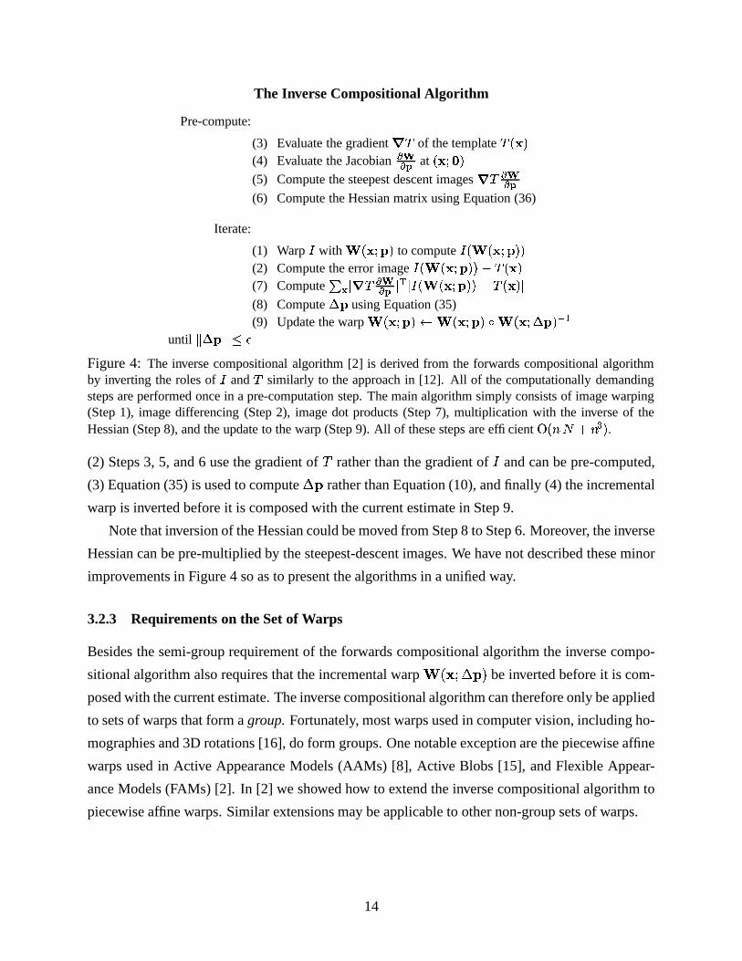
until '(�&�)'+*-,Figure 4: The inverse compositional algorithm [2] is derived from the forwards compositional algorithmby inverting the roles of � and � similarly to the approach in [12]. All of the computationally demandingsteps are performed once in a pre-computation step. The main algorithm simply consists of image warping(Step 1), image differencing (Step 2), image dot products (Step 7), multiplication with the inverse of theHessian (Step 8), and the update to the warp (Step 9). All of these steps are efficient � �� #�� L .(2) Steps 3, 5, and 6 use the gradient of

�rather than the gradient of � and can be pre-computed,

(3) Equation (35) is used to compute � $ rather than Equation (10), and finally (4) the incremental

warp is inverted before it is composed with the current estimate in Step 9.

Note that inversion of the Hessian could be moved from Step 8 to Step 6. Moreover, the inverse

Hessian can be pre-multiplied by the steepest-descent images. We have not described these minor

improvements in Figure 4 so as to present the algorithms in a unified way.


Besides the semi-group requirement of the forwards compositional algorithm the inverse compo-

sitional algorithm also requires that the incremental warp ��#" � $&� be inverted before it is com-

posed with the current estimate. The inverse compositional algorithm can therefore only be applied

to sets of warps that form a group. Fortunately, most warps used in computer vision, including ho-

mographies and 3D rotations [16], do form groups. One notable exception are the piecewise affine

warps used in Active Appearance Models (AAMs) [8], Active Blobs [15], and Flexible Appear-

ance Models (FAMs) [2]. In [2] we showed how to extend the inverse compositional algorithm to

piecewise affine warps. Similar extensions may be applicable to other non-group sets of warps.

14

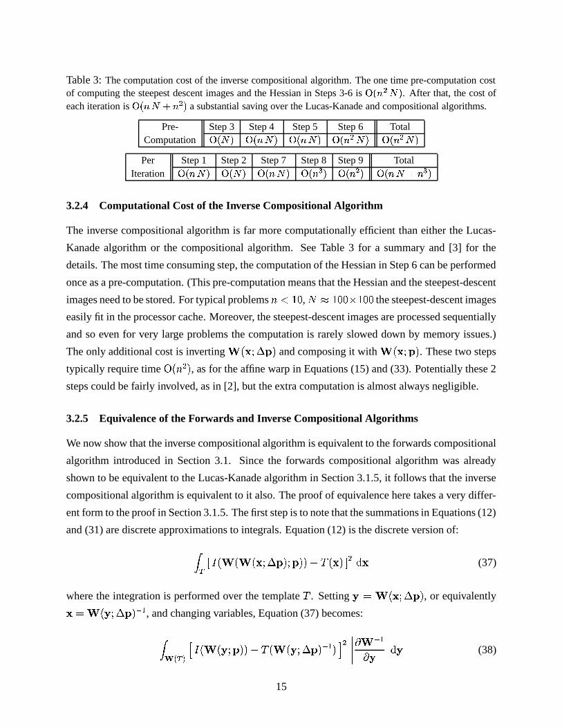
Table 3: The computation cost of the inverse compositional algorithm. The one time pre-computation costof computing the steepest descent images and the Hessian in Steps 3-6 is �&�� = � . After that, the cost ofeach iteration is � �� #�� = a substantial saving over the Lucas-Kanade and compositional algorithms.

Pre- Step 3 Step 4 Step 5 Step 6 TotalComputation �&� � � �� = � �&�� = �

Per Step 1 Step 2 Step 7 Step 8 Step 9 TotalIteration � �� &� � � �� L � �� = � �� #�� L

3.2.4 Computational Cost of the Inverse Compositional Algorithm

The inverse compositional algorithm is far more computationally efficient than either the Lucas-

Kanade algorithm or the compositional algorithm. See Table 3 for a summary and [3] for the

details. The most time consuming step, the computation of the Hessian in Step 6 can be performed

once as a pre-computation. (This pre-computation means that the Hessian and the steepest-descent

images need to be stored. For typical problems \�� "), � � � )�) � �")�) the steepest-descent images

easily fit in the processor cache. Moreover, the steepest-descent images are processed sequentially

and so even for very large problems the computation is rarely slowed down by memory issues.)

The only additional cost is inverting �!�#" � $4� and composing it with �!�#"%$&�. These two steps

typically require time � � \ = � , as for the affine warp in Equations (15) and (33). Potentially these 2

steps could be fairly involved, as in [2], but the extra computation is almost always negligible.

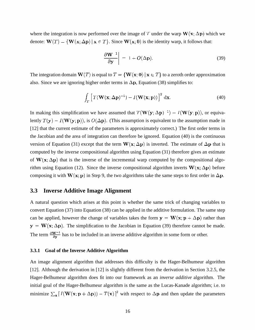
3.2.5 Equivalence of the Forwards and Inverse Compositional Algorithms

We now show that the inverse compositional algorithm is equivalent to the forwards compositional

algorithm introduced in Section 3.1. Since the forwards compositional algorithm was already

shown to be equivalent to the Lucas-Kanade algorithm in Section 3.1.5, it follows that the inverse

compositional algorithm is equivalent to it also. The proof of equivalence here takes a very differ-

ent form to the proof in Section 3.1.5. The first step is to note that the summations in Equations (12)

and (31) are discrete approximations to integrals. Equation (12) is the discrete version of:

�� _ � � � ��#" � $&� "%$&�%��a �8�!��2b =�� (37)

where the integration is performed over the template�

. Setting � ��#" � $&� , or equivalently� � � " � $4� / * , and changing variables, Equation (37) becomes:

� �� "%$&�%��a �� " � $&� / * �� =�� / *� �

�� (38)

15

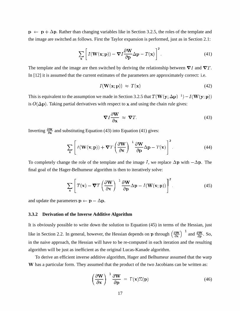
where the integration is now performed over the image of�

under the warp ��#" � $&� which we

denote: ��;�� 3" � $4�� . Since ��#"��C�is the identity warp, it follows that:

�� / *� �

�� N7� � � $4��- (39)

The integration domain ��;�is equal to

� � �!�#"��C�� 5��to a zeroth order approximation

also. Since we are ignoring higher order terms in � $ , Equation (38) simplifies to:

�� #" � $&� / * �Ja � � �!�#"%$&�%� � = � �3-(40)

In making this simplification we have assumed that�� " � $4� / * �Na � � � � "%$&�%� , or equiva-

lently�� a � � � � "G$4�G� , is

� � � $&� . (This assumption is equivalent to the assumption made in

[12] that the current estimate of the parameters is approximately correct.) The first order terms in

the Jacobian and the area of integration can therefore be ignored. Equation (40) is the continuous

version of Equation (31) except that the term �!�#" � $&� is inverted. The estimate of � $ that is

computed by the inverse compositional algorithm using Equation (31) therefore gives an estimate

of ��#" � $&� that is the inverse of the incremental warp computed by the compositional algo-

rithm using Equation (12). Since the inverse compositional algorithm inverts ��3" � $4� before

composing it with ��#"%$&�in Step 9, the two algorithms take the same steps to first order in � $ .

3.3 Inverse Additive Image Alignment

A natural question which arises at this point is whether the same trick of changing variables to

convert Equation (37) into Equation (38) can be applied in the additive formulation. The same step

can be applied, however the change of variables takes the form � �!�#"%$<7 � $&� rather than� ��#" � $&� . The simplification to the Jacobian in Equation (39) therefore cannot be made.

The term�� !�� has to be included in an inverse additive algorithm in some form or other.

3.3.1 Goal of the Inverse Additive Algorithm

An image alignment algorithm that addresses this difficulty is the Hager-Belhumeur algorithm

[12]. Although the derivation in [12] is slightly different from the derivation in Section 3.2.5, the

Hager-Belhumeur algorithm does fit into our framework as an inverse additive algorithm. The

initial goal of the Hager-Belhumeur algorithm is the same as the Lucas-Kanade algorithm; i.e. to

minimize �^ _ � � �!�#"%$V7 � $4�G�Ja �8�!��2b = with respect to � $ and then update the parameters

16

$ � $ 7 � $Q- Rather than changing variables like in Section 3.2.5, the roles of the template and

the image are switched as follows. First the Taylor expansion is performed, just as in Section 2.1:] ^ � � ��3"%$4�G� 7�� $ � $9a �� = - (41)

The template and the image are then switched by deriving the relationship between� � and

�9�.

In [12] it is assumed that the current estimates of the parameters are approximately correct: i.e.� � ��3"%$4�G�� (42)

This is equivalent to the assumption we made in Section 3.2.5 that�� " � $4� / * � a � � � � "%$&�%�

is� � � $&� . Taking partial derivatives with respect to

�and using the chain rule gives:

� � � � � � �9� -(43)

Inverting�� ^ and substituting Equation (43) into Equation (41) gives:] ^�� !�#"%$&�%� 7 �9� 6 � � � >

/ * � � $ � $<a �� = - (44)

To completely change the role of the template and the image � , we replace � $ witha � $ . The

final goal of the Hager-Belhumeur algorithm is then to iteratively solve:]X^ �� 8�!��C7 �9�`6 � � � >/ * � � $ � $9a � � �!�#"%$&�%�� = - (45)

and update the parameters$ � $9a � $ .

3.3.2 Derivation of the Inverse Additive Algorithm

It is obviously possible to write down the solution to Equation (45) in terms of the Hessian, just

like in Section 2.2. In general, however, the Hessian depends on$

through � �� ^�� / * and�� . So,

in the naive approach, the Hessian will have to be re-computed in each iteration and the resulting

algorithm will be just as inefficient as the original Lucas-Kanade algorithm.

To derive an efficient inverse additive algorithm, Hager and Belhumeur assumed that the warp has a particular form. They assumed that the product of the two Jacobians can be written as:6 � � � >/ * � � $ &�� $&�

(46)

17

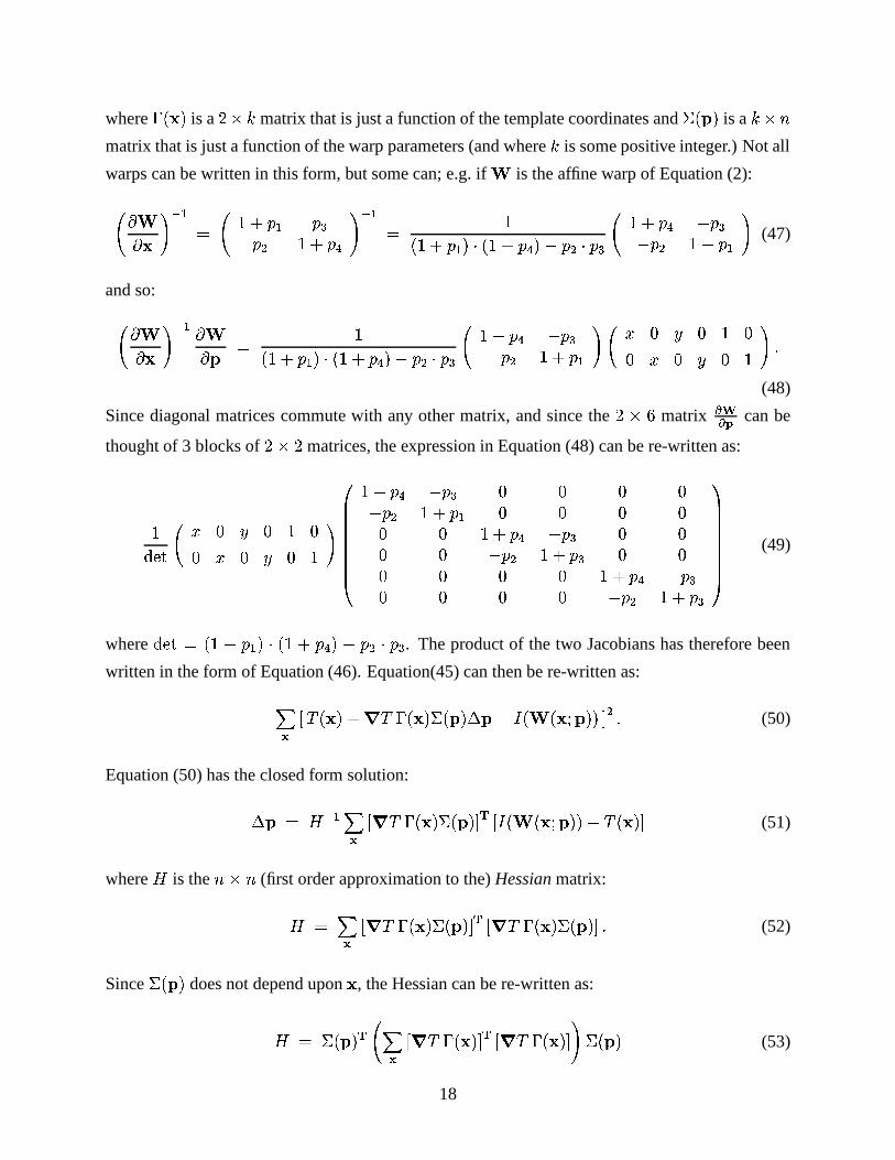
where&��

is a� �� matrix that is just a function of the template coordinates and

�!$4�is a � � \

matrix that is just a function of the warp parameters (and where � is some positive integer.) Not all

warps can be written in this form, but some can; e.g. if is the affine warp of Equation (2):

6 � � � >/ * 6 �Q7<(H* (�L(�= �479(1O > / * ��G�N79(H* �JI2�G�N79(1O,�Ja (�=&I�(�L 6 �N79( O a&(�La&(�= �N79(H*�> (47)

and so:6 � � � >/ * � � $ ��G�N79(H* �JI2�G�N79(1O,�Ja (�=&I�(�L 6 �N79( O a&(�La&(�= �N79(H* > 6 � ) � ) � )) � ) � ) � > -

(48)

Since diagonal matrices commute with any other matrix, and since the� �� matrix

�� can be

thought of 3 blocks of� � � matrices, the expression in Equation (48) can be re-written as:

�� 6 � ) � ) � )) � ) � ) � > RSSSSSSSST�Q7<(1O a&(�L ) ) ) )a&(�= �Q7<(H* ) ) ) )) ) �N7<(1O a&(�L ) )) ) a&(�= �N7<(�L ) )) ) ) ) �N7<(1O a&(�L) ) ) ) a&(�= �N79(1L

UXWWWWWWWWY (49)

where�� 7 ( *D�#I1�G� 7 (1O/�#a (�= I/(�L

. The product of the two Jacobians has therefore been

written in the form of Equation (46). Equation(45) can then be re-written as:]X^ _ ��C7 �9� &�� $&� � $9a � � ��3"%$4�G�2b = -(50)

Equation (50) has the closed form solution:

� $� . / * ] ^ _ �� &�� $&�Fb � _ � � �!�#"%$&�%� a�8�!��Fb(51)

where.

is the \9� \ (first order approximation to the) Hessian matrix:

. ] ^ _ �9� &�� $&�Fb � _ � � 4�!�� !$4�Eb -(52)

Since ��$&�

does not depend upon�

, the Hessian can be re-written as:

. �!$4� � 6 ]�^`_ �9� 4�!��Fb � _ �9� &��Eb > ��$&� (53)

18

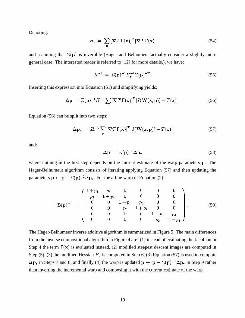
Denoting: .�� ] ^ _ �� &��Eb � _ �9� &��Eb(54)

and assuming that ��$&�

is invertible (Hager and Belhumeur actually consider a slightly more

general case. The interested reader is referred to [12] for more details.), we have:

. / * ��$&� / * . / *� ��$&� / � -(55)

Inserting this expression into Equation (51) and simplifying yields:

� $� ��$&� / * . / *� ] ^ _ � � &��Fb � _ � � �!�#"%$&�%� a ��!��Fb -(56)

Equation (56) can be split into two steps:

� $�� . / *� ] ^ _ � � &��Fb � _ � � �!�#"%$&�%� a ��!��Fb(57)

and: � $� �!$4� / * � $�� (58)

where nothing in the first step depends on the current estimate of the warp parameters$

. The

Hager-Belhumeur algorithm consists of iterating applying Equation (57) and then updating the

parameters$ � $9a ��$&� / * � $�� . For the affine warp of Equation (2):

�!$4�(/ * RSSSSSSSST�N79(H* (�L ) ) ) )(�= �N79(1O ) ) ) )) ) �N79(H* (�L ) )) ) (�= �Q7<(1O ) )) ) ) ) �Q7<(H* (�L) ) ) ) (�= �Q7<(1O

UXWWWWWWWWY-

(59)

The Hager-Belhumeur inverse additive algorithm is summarized in Figure 5. The main differences

from the inverse compositional algorithm in Figure 4 are: (1) instead of evaluating the Jacobian in

Step 4 the term&��

is evaluated instead, (2) modified steepest descent images are computed in

Step (5), (3) the modified Hessian.��

is computed in Step 6, (3) Equation (57) is used to compute� $�� in Steps 7 and 8, and finally (4) the warp is updated$�� $ a ��$&� / * � $�� in Step 9 rather

than inverting the incremental warp and composing it with the current estimate of the warp.

19

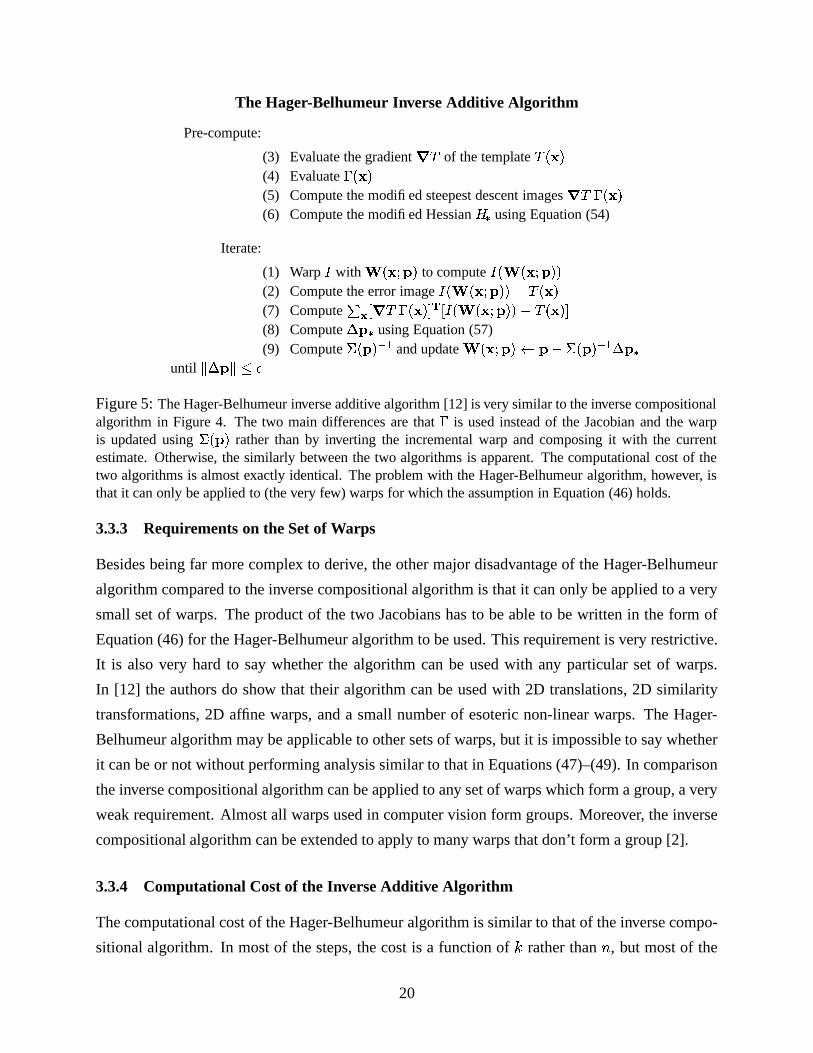
The Hager-Belhumeur Inverse Additive Algorithm

Pre-compute:

(3) Evaluate the gradient � � of the template ��(4) Evaluate

� ��(5) Compute the modified steepest descent images � � � ��(6) Compute the modified Hessian �

�

using Equation (54)

Iterate:

(1) Warp � with �� to compute �� (2) Compute the error image �� (7) Compute �

^ ��

(8) Compute �� using Equation (57)(9) Compute � � � / * and update �� / * �&� �

until '(�&�)'+*-,Figure 5: The Hager-Belhumeur inverse additive algorithm [12] is very similar to the inverse compositionalalgorithm in Figure 4. The two main differences are that

�is used instead of the Jacobian and the warp

is updated using � � �� rather than by inverting the incremental warp and composing it with the currentestimate. Otherwise, the similarly between the two algorithms is apparent. The computational cost of thetwo algorithms is almost exactly identical. The problem with the Hager-Belhumeur algorithm, however, isthat it can only be applied to (the very few) warps for which the assumption in Equation (46) holds.


Besides being far more complex to derive, the other major disadvantage of the Hager-Belhumeur

algorithm compared to the inverse compositional algorithm is that it can only be applied to a very

small set of warps. The product of the two Jacobians has to be able to be written in the form of

Equation (46) for the Hager-Belhumeur algorithm to be used. This requirement is very restrictive.

It is also very hard to say whether the algorithm can be used with any particular set of warps.

In [12] the authors do show that their algorithm can be used with 2D translations, 2D similarity

transformations, 2D affine warps, and a small number of esoteric non-linear warps. The Hager-

Belhumeur algorithm may be applicable to other sets of warps, but it is impossible to say whether

it can be or not without performing analysis similar to that in Equations (47)–(49). In comparison

the inverse compositional algorithm can be applied to any set of warps which form a group, a very

weak requirement. Almost all warps used in computer vision form groups. Moreover, the inverse

compositional algorithm can be extended to apply to many warps that don’t form a group [2].

3.3.4 Computational Cost of the Inverse Additive Algorithm

The computational cost of the Hager-Belhumeur algorithm is similar to that of the inverse compo-

sitional algorithm. In most of the steps, the cost is a function of � rather than \ , but most of the

20

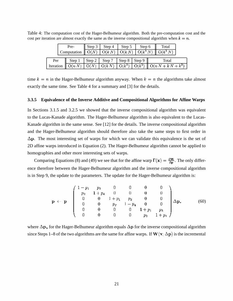
Table 4: The computation cost of the Hager-Belhumeur algorithm. Both the pre-computation cost and thecost per iteration are almost exactly the same as the inverse compositional algorithm when �� .

Pre- Step 3 Step 4 Step 5 Step 6 TotalComputation � � � � �� &�� = � � �� = �

Per Step 1 Step 2 Step 7 Step 8 Step 9 TotalIteration � �� &�� L � �� = � �� #�� #�� L

time � \ in the Hager-Belhumeur algorithm anyway. When � \ the algorithms take almost

exactly the same time. See Table 4 for a summary and [3] for the details.

3.3.5 Equivalence of the Inverse Additive and Compositional Algorithms for Affine Warps

In Sections 3.1.5 and 3.2.5 we showed that the inverse compositional algorithm was equivalent

to the Lucas-Kanade algorithm. The Hager-Belhumeur algorithm is also equivalent to the Lucas-

Kanade algorithm in the same sense. See [12] for the details. The inverse compositional algorithm

and the Hager-Belhumeur algorithm should therefore also take the same steps to first order in� $ . The most interesting set of warps for which we can validate this equivalence is the set of

2D affine warps introduced in Equation (2). The Hager-Belhumeur algorithm cannot be applied to

homographies and other more interesting sets of warps.

Comparing Equations (8) and (49) we see that for the affine warp&��3 �� . The only differ-

ence therefore between the Hager-Belhumeur algorithm and the inverse compositional algorithm

is in Step 9, the update to the parameters. The update for the Hager-Belhumeur algorithm is:

$�� $ a RSSSSSSSST�N79(H* (�L ) ) ) )(�= �479(1O ) ) ) )) ) �Q7<(H* (�L ) )) ) (�= �Q7<(1O ) )) ) ) ) �N7<(H* (�L) ) ) ) (�= �N7<(1O

UXWWWWWWWWY � $�� (60)

where � $�� for the Hager-Belhumeur algorithm equals � $ for the inverse compositional algorithm

since Steps 1–8 of the two algorithms are the same for affine warps. If �!�#" � $4� is the incremental

21

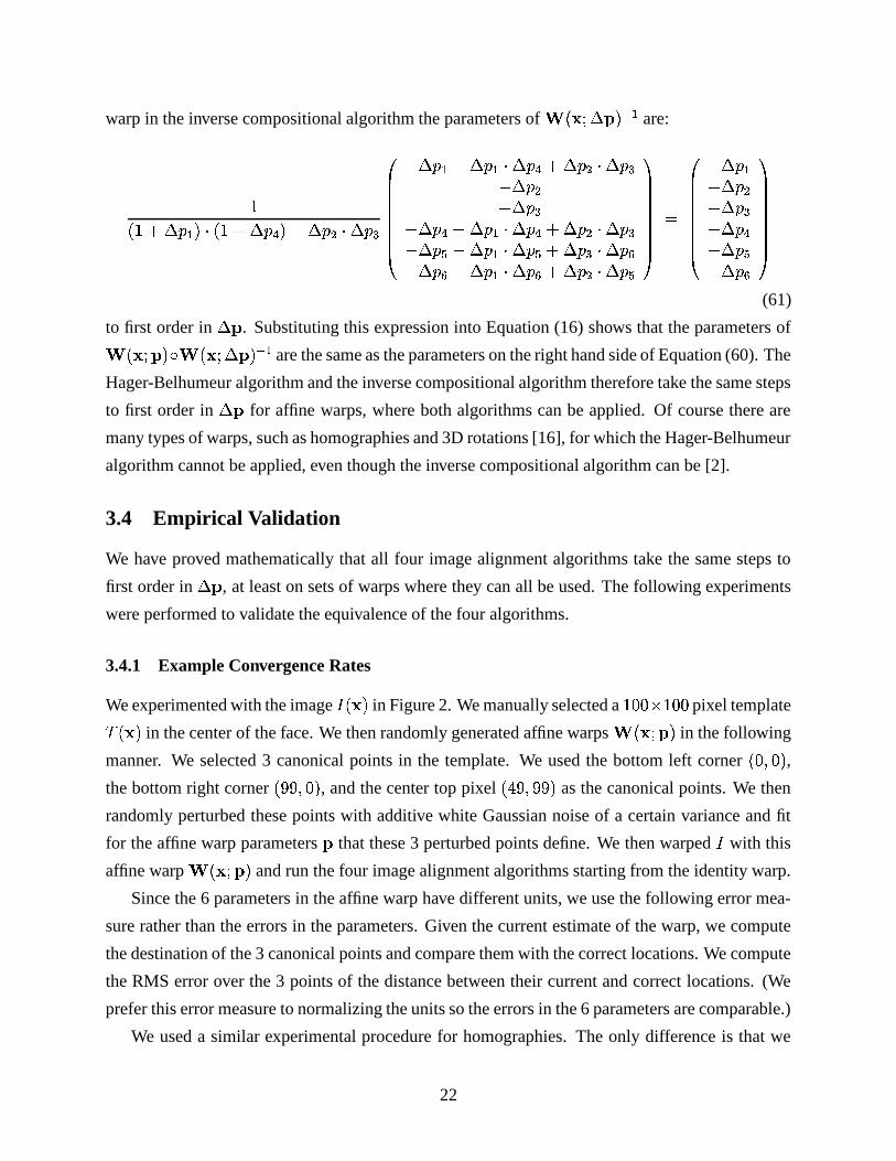
warp in the inverse compositional algorithm the parameters of �!�#" � $4� / * are:

��G�N7 � (H*D�JI2��N7 � (1O/�Ja � (�=4I � (�L RSSSSSSSSTa � (H*#a � (H*#I � ( O#7 � (1=4I � (�La � (�=a � (�La � (1ONa � (H*#I � ( O#7 � (1=4I � (�La � (�M4a � (H*#I � (1M37 � (1L4I � (�Pa � (�P4a � (H*#I � (1P37 � (1=4I � (�M

U WWWWWWWWY RSSSSSSSST

a � (H*a � (�=a � (�La � (1Oa � (�Ma � (�PU WWWWWWWWY(61)

to first order in � $ . Substituting this expression into Equation (16) shows that the parameters of �!�#"%$&� � ��3" � $4� / * are the same as the parameters on the right hand side of Equation (60). The

Hager-Belhumeur algorithm and the inverse compositional algorithm therefore take the same steps

to first order in � $ for affine warps, where both algorithms can be applied. Of course there are

many types of warps, such as homographies and 3D rotations [16], for which the Hager-Belhumeur

algorithm cannot be applied, even though the inverse compositional algorithm can be [2].

3.4 Empirical Validation

We have proved mathematically that all four image alignment algorithms take the same steps to

first order in � $ , at least on sets of warps where they can all be used. The following experiments

were performed to validate the equivalence of the four algorithms.

3.4.1 Example Convergence Rates

We experimented with the image � �!�� in Figure 2. We manually selected a�")�) � �")�) pixel template��

in the center of the face. We then randomly generated affine warps ��#"G$4�in the following

manner. We selected 3 canonical points in the template. We used the bottom left corner� ) ��) �

,

the bottom right corner�� ) �

, and the center top pixel��

as the canonical points. We then

randomly perturbed these points with additive white Gaussian noise of a certain variance and fit

for the affine warp parameters$

that these 3 perturbed points define. We then warped � with this

affine warp ��#"%$&�and run the four image alignment algorithms starting from the identity warp.

Since the 6 parameters in the affine warp have different units, we use the following error mea-

sure rather than the errors in the parameters. Given the current estimate of the warp, we compute

the destination of the 3 canonical points and compare them with the correct locations. We compute

the RMS error over the 3 points of the distance between their current and correct locations. (We

prefer this error measure to normalizing the units so the errors in the 6 parameters are comparable.)

We used a similar experimental procedure for homographies. The only difference is that we

22

used 4 canonical points at the corners of the template, bottom left� ) � ) �

, bottom right�� ) �

, top

left� ) ��

, and top right��

rather than the 3 canonical points used for affine warps.

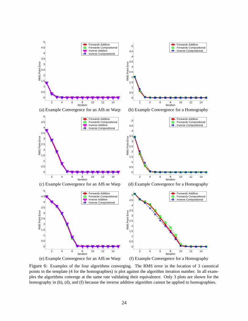
In Figure 6 we include examples of the algorithms converging. The RMS error in the canonical

point locations is plot against the iteration number. In Figures 6(a), (c), and (e) we plot results for

affine warps. In Figures 6(b), (d), and (f) we plot results for homographies. As can be seen, the

algorithms converge at the same rate validating their equivalence. The inverse additive algorithm

cannot be used for homographies and so only 3 curves are shown in Figures 6(b), (d), and (f). See

Appendix A for the derivation of the inverse compositional algorithm for the homography.

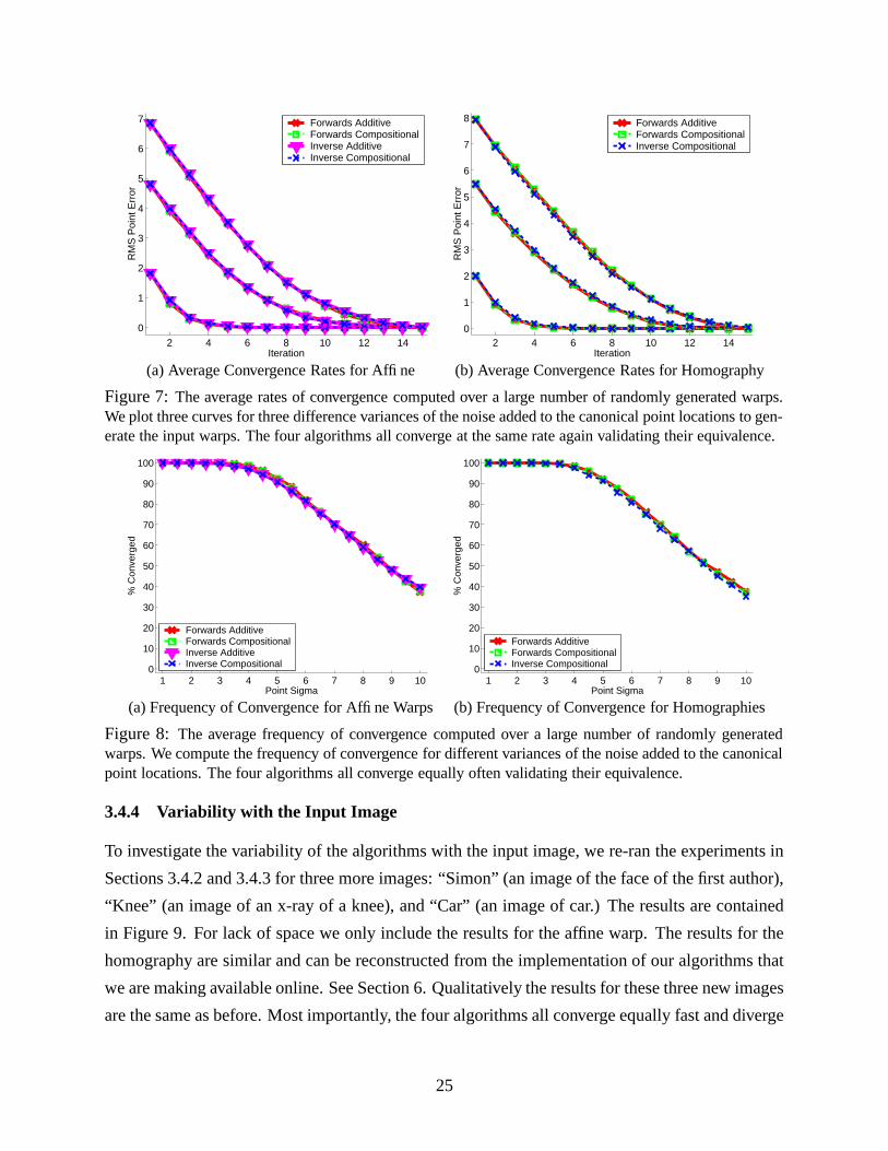
3.4.2 Average Rates of Convergence

We also computed the average rate of convergence over a large number (5000) of randomly gen-

erated inputs. To avoid the results being biased by cases where one or more of the algorithms

diverged, we checked that all 4 algorithms converged before including the sample in the average.

We say that an algorithm has diverged in this experiment if the final RMS error in the canonical

point location is larger than it was in the input. The average rates of convergence are shown in Fig-

ure 7 where we plot three curves for three different variances of the noise added to the canonical

point locations. As can be seen, the 4 algorithms (3 for the homography) all converge at almost

exactly the same rate, again validating the equivalence of the four algorithms. The algorithms all

require between 5 and 15 iterations to converge depending on the magnitude of the initial error.

(Faster convergence can be obtained by processing hierarchically on a Gaussian pyramid [4].)

3.4.3 Average Frequency of Convergence

What about the case that the algorithms diverge? We ran a second similar experiment over 5000

randomly generated inputs. In this case, we counted the number of times that each algorithm

converged. In this second experiment, we say that an algorithm converged if after 15 iterations the

RMS error in the canonical point locations is less than 1.0 pixels. We computed the percentage

of times that each algorithm converged for various different variances of the noise added to the

canonical point locations. The results are shown in Figure 8. Again, the four algorithms all perform

much the same, validating their equivalence. When the perturbation to the canonical point locations

is less than about 4.0 pixels, all four algorithms converge almost always. Above that amount of

perturbation the frequency of convergence rapidly decreases.

None of the algorithms used a multi-scale pyramid to increase their robustness. This extension

could be applied to all of the algorithms. Our goal was only to validate the equivalence of the base

algorithms. The effect of using a multi-scale pyramid will be studied in a future paper.

23

2 4 6 8 10 12 14

0

0.5

1

1.5

2

2.5

3

3.5

4

4.5

5

Iteration

RM

S P

oint

Err

or

Forwards AdditiveForwards CompositionalInverse AdditiveInverse Compositional

2 4 6 8 10 12 14

0

0.5

1

1.5

2

2.5

3

3.5

4

4.5

5

Iteration

RM

S P

oint

Err

or

Forwards AdditiveForwards CompositionalInverse Compositional

(a) Example Convergence for an Affine Warp (b) Example Convergence for a Homography

2 4 6 8 10 12 14

0

0.5

1

1.5

2

2.5

3

3.5

4

4.5

5

Iteration

RM

S P

oint

Err

or


2 4 6 8 10 12 14

0

0.5

1

1.5

2

2.5

3

3.5

4

4.5

5

Iteration

RM

S P

oint

Err

or


(c) Example Convergence for an Affine Warp (d) Example Convergence for a Homography

2 4 6 8 10 12 14

0

0.5

1

1.5

2

2.5

3

3.5

4

4.5

5

Iteration

RM

S P

oint

Err

or


2 4 6 8 10 12 14

0

0.5

1

1.5

2

2.5

3

3.5

4

4.5

5

Iteration

RM

S P

oint

Err

or


(e) Example Convergence for an Affine Warp (f) Example Convergence for a Homography

Figure 6: Examples of the four algorithms converging. The RMS error in the location of 3 canonicalpoints in the template (4 for the homographies) is plot against the algorithm iteration number. In all exam-ples the algorithms converge at the same rate validating their equivalence. Only 3 plots are shown for thehomography in (b), (d), and (f) because the inverse additive algorithm cannot be applied to homographies.

24

2 4 6 8 10 12 14

0

1

2

3

4

5

6

7

Iteration

RM

S P

oint

Err

orForwards AdditiveForwards CompositionalInverse AdditiveInverse Compositional

2 4 6 8 10 12 140

1

2

3

4

5

6

7

8

Iteration

RM

S P

oint

Err

or


(a) Average Convergence Rates for Affine (b) Average Convergence Rates for Homography

Figure 7: The average rates of convergence computed over a large number of randomly generated warps.We plot three curves for three difference variances of the noise added to the canonical point locations to gen-erate the input warps. The four algorithms all converge at the same rate again validating their equivalence.

1 2 3 4 5 6 7 8 9 100

10

20

30

40

50

60

70

80

90

100

Point Sigma

% C

onve

rged


1 2 3 4 5 6 7 8 9 100

10

20

30

40

50

60

70

80

90

100

Point Sigma

% C

onve

rged


(a) Frequency of Convergence for Affine Warps (b) Frequency of Convergence for Homographies

Figure 8: The average frequency of convergence computed over a large number of randomly generatedwarps. We compute the frequency of convergence for different variances of the noise added to the canonicalpoint locations. The four algorithms all converge equally often validating their equivalence.

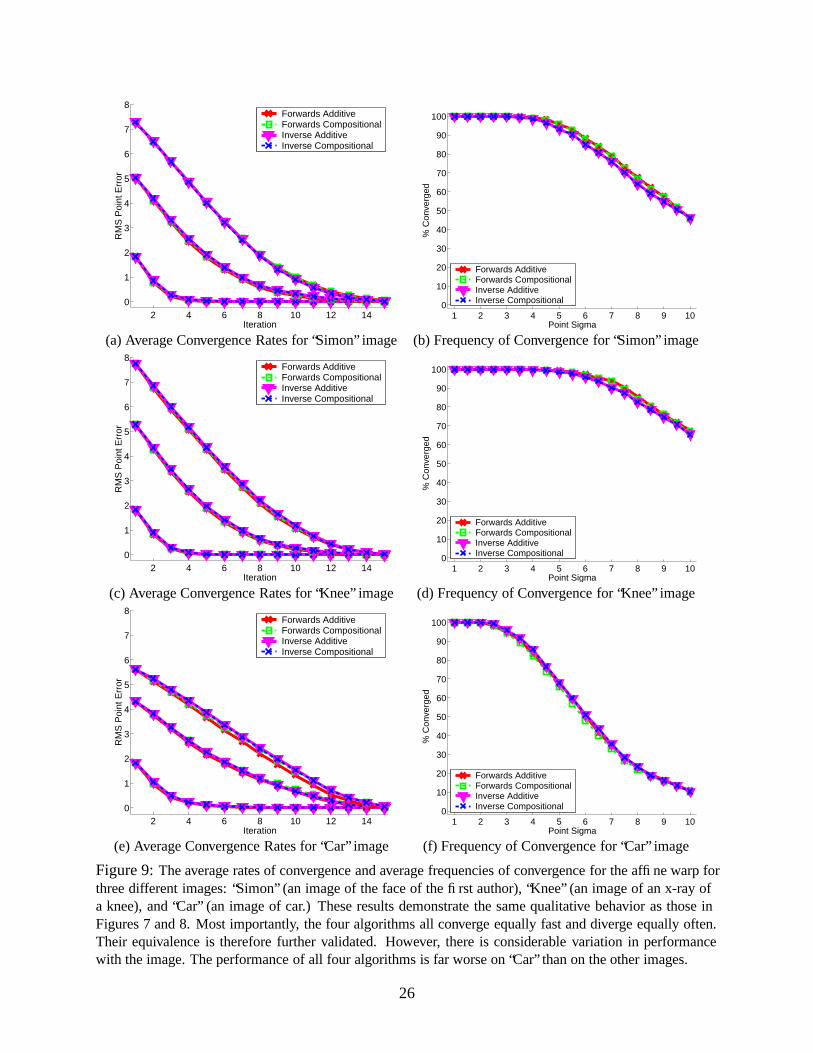
3.4.4 Variability with the Input Image

To investigate the variability of the algorithms with the input image, we re-ran the experiments in

Sections 3.4.2 and 3.4.3 for three more images: “Simon” (an image of the face of the first author),

“Knee” (an image of an x-ray of a knee), and “Car” (an image of car.) The results are contained

in Figure 9. For lack of space we only include the results for the affine warp. The results for the

homography are similar and can be reconstructed from the implementation of our algorithms that

we are making available online. See Section 6. Qualitatively the results for these three new images

are the same as before. Most importantly, the four algorithms all converge equally fast and diverge

25

2 4 6 8 10 12 140

1

2

3

4

5

6

7

8

Iteration

RM

S P

oint

Err


1 2 3 4 5 6 7 8 9 100

10

20

30

40

50

60

70

80

90

100

Point Sigma

% C

onve

rged


(a) Average Convergence Rates for “Simon” image (b) Frequency of Convergence for “Simon” image

2 4 6 8 10 12 140

1

2

3

4

5

6

7

8

Iteration

RM

S P

oint

Err

or


1 2 3 4 5 6 7 8 9 100

10

20

30

40

50

60

70

80

90

100

Point Sigma

% C

onve

rged


(c) Average Convergence Rates for “Knee” image (d) Frequency of Convergence for “Knee” image

2 4 6 8 10 12 140

1

2

3

4

5

6

7

8

Iteration

RM

S P

oint

Err

or


1 2 3 4 5 6 7 8 9 100

10

20

30

40

50

60

70

80

90

100

Point Sigma

% C

onve

rged


(e) Average Convergence Rates for “Car” image (f) Frequency of Convergence for “Car” image

Figure 9: The average rates of convergence and average frequencies of convergence for the affine warp forthree different images: “Simon” (an image of the face of the first author), “Knee” (an image of an x-ray ofa knee), and “Car” (an image of car.) These results demonstrate the same qualitative behavior as those inFigures 7 and 8. Most importantly, the four algorithms all converge equally fast and diverge equally often.Their equivalence is therefore further validated. However, there is considerable variation in performancewith the image. The performance of all four algorithms is far worse on “Car” than on the other images.

26

equally often. Their equivalence is therefore further validated. There is considerable variation

in performance across the images, however. In particular, the performance of all four algorithms

for the “Car” image is far worse than for the other three images, both in terms of average rate of

convergence and in terms of average frequency of divergence.

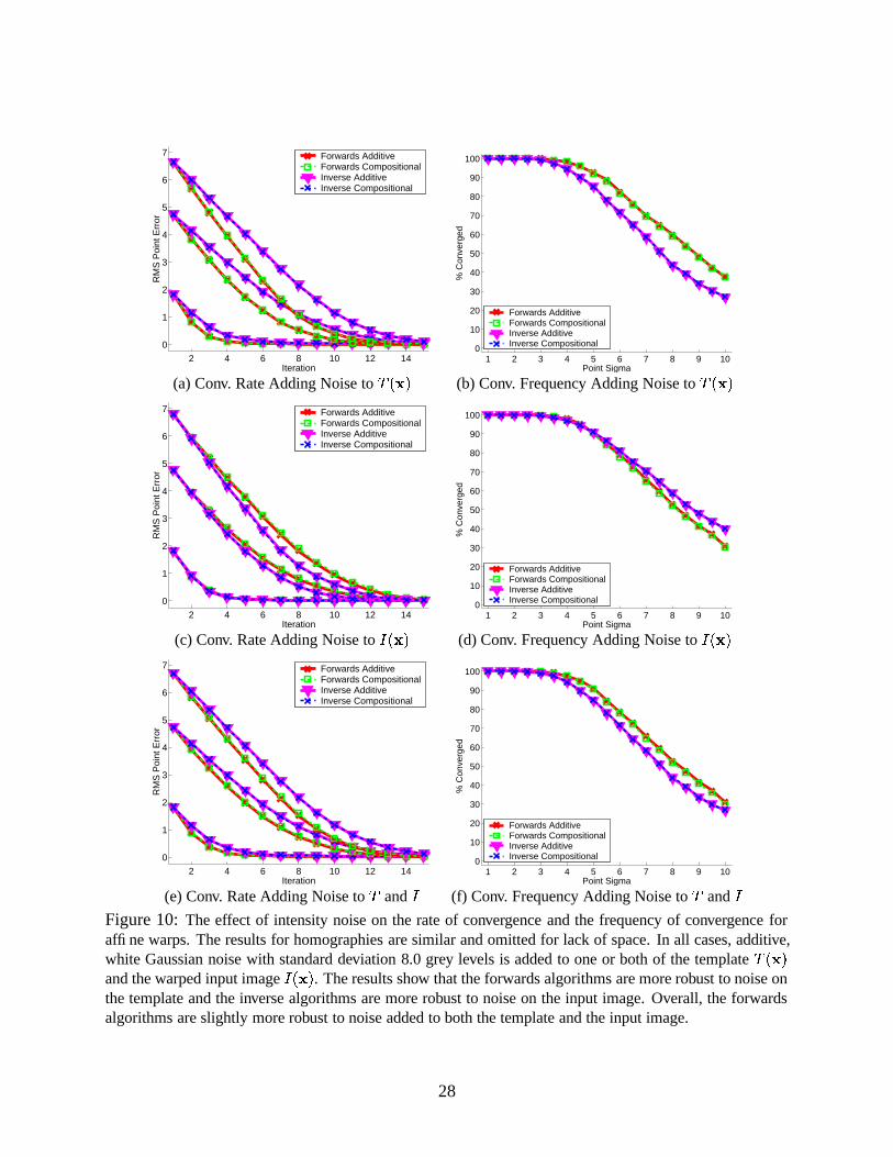
3.4.5 The Effect of Additive Intensity Noise

The results that we have presented so far have not included any noise on the images themselves

(just on the canonical point locations which is not really noise but just a way of generating random

warps.) The image � �!�� is warped with �!�#"%$&�to generate the input image, a process which

introduces a very small amount of re-sampling noise, but that re-sampling noise is negligible.

We repeated the above experiments, but with additive, white Gaussian noise added to the im-

ages. We considered 3 cases: (1) noise added to the image � �� , (2) noise added to the template��, and (3) noise added to both � �� and

�� -The results for additive noise with standard

deviation 8 grey levels is shown in Figure 10.

The first thing to note is that noise breaks the equivalence of the forwards and inverse algo-

rithms. This is not too surprising. In the proof of equivalence it is assumed that�� a � � � � "%$4�G�

is� � � $&� . This is not true in the presence of noise. Since the forwards algorithms compute the gra-

dient of � and the inverse algorithms compute the gradient of�

, it is not surprising that when noise

is added to � the inverse algorithms converge better (faster and more frequently), and conversely

when noise is added to�

the forwards algorithms converge better. When equal noise is added

to both images, the forwards algorithms perform marginally better than the inverse algorithms

because the inverse algorithms are only first-order approximations to the forwards algorithms.

Overall we conclude that the forwards algorithms are ever so slightly more robust to additive

noise. However, in many applications such as in face modeling [2], the template image�8�!��

can

be computed as an average of a large number of images and should be less noisy than the input

image � �� . In such cases, the inverse algorithms will be more robust to noise.

3.4.6 Timing Results

We implemented the four algorithms in Matlab. The Matlab implementation of image warping

(Step 1, also used in Step 3 in the forwards additive algorithm) is very slow. Hence we re-

implemented that step in “C.” The timing results for the 6-parameter affine warp using a� )�) � �")�)

pixel grey-scale template on a 933MHz Pentium-IV are included in Table 5. As can be seen, the

two inverse algorithms shift much of the computation into pre-computation and so are far faster per

iteration. The forwards compositional algorithm is also somewhat faster than the forwards additive

27

2 4 6 8 10 12 14

0

1

2

3

4

5

6

7

Iteration

RM

S P

oint

Err


1 2 3 4 5 6 7 8 9 100

10

20

30

40

50

60

70

80

90

100

Point Sigma

% C

onve

rged


(a) Conv. Rate Adding Noise to �� (b) Conv. Frequency Adding Noise to ��

2 4 6 8 10 12 14

0

1

2

3

4

5

6

7

Iteration

RM

S P

oint

Err

or


1 2 3 4 5 6 7 8 9 100

10

20

30

40

50

60

70

80

90

100

Point Sigma

% C

onve

rged


(c) Conv. Rate Adding Noise to �� (d) Conv. Frequency Adding Noise to ��

2 4 6 8 10 12 14

0

1

2

3

4

5

6

7

Iteration

RM

S P

oint

Err

or


1 2 3 4 5 6 7 8 9 100

10

20

30

40

50

60

70

80

90

100

Point Sigma

% C

onve

rged


(e) Conv. Rate Adding Noise to � and � (f) Conv. Frequency Adding Noise to � and �Figure 10: The effect of intensity noise on the rate of convergence and the frequency of convergence foraffine warps. The results for homographies are similar and omitted for lack of space. In all cases, additive,white Gaussian noise with standard deviation 8.0 grey levels is added to one or both of the template ��and the warped input image �� . The results show that the forwards algorithms are more robust to noise onthe template and the inverse algorithms are more robust to noise on the input image. Overall, the forwardsalgorithms are slightly more robust to noise added to both the template and the input image.

28

Table 5: Timing results for our Matlab implementation of the four algorithms in milliseconds. These resultsare for the 6-parameter affine warp using a

��pixel template on a 933MHz Pentium-IV.

Pre-computation:

Step 3 Step 4 Step 5 Step 6 Total

Forwards Additive (FA) - - - - 0.0Forwards Compositional (FC) - 17.4 - - 17.4Inverse Additive (IA) 8.30 17.1 27.5 37.0 89.9Inverse Compositional (IC) 8.31 17.1 27.5 37.0 90.0

Per Iteration:

Step 1 Step 2 Step 3 Step 4 Step 5 Step 6 Step 7 Step 8 Step 9 Total

FA 1.88 0.740 36.1 17.4 27.7 37.2 6.32 0.111 0.108 127FC 1.88 0.736 8.17 - 27.6 37.0 6.03 0.106 0.253 81.7IA 1.79 0.688 - - - - 6.22 0.106 0.624 9.43IC 1.79 0.687 - - - - 6.22 0.106 0.409 9.21

algorithm since it does not need to warp the image gradients in Step 3 and the image gradients are

computed on the template rather than the input image which is generally larger.

3.5 Summary

We have outlined three approaches to image alignment beyond the original forwards additive

Lucas-Kanade algorithm. We refer to these approaches as the forwards compositional, the in-

verse additive, and the inverse compositional algorithms. In Sections 3.1.5, 3.2.5, and 3.3.5 we

proved that all four algorithms are equivalent in the sense that they take the same steps in each

iteration to first order in � $ . In Section 3.4 we validated this equivalence empirically.

The four algorithms do differ, however, in two other respects. See Table 6 for a summary.

Although the computational requirements of the two forwards algorithms are almost identical and

the computational requirements of the two inverse algorithms are also almost identical, the two

inverse algorithms are far more efficient than the two forwards algorithms. On the other hand,

the forwards additive algorithm can be applied to any type of warp, the forwards compositional

algorithm can only be applied to sets of warps that form semi-groups, and the inverse compositional

algorithm can only be applied sets of warps that form groups. The inverse additive algorithm can

be applied to very few warps, mostly simple 2D linear warps such as translations and affine warps.

A natural question which arises at this point is which of the four algorithms should be used.

29

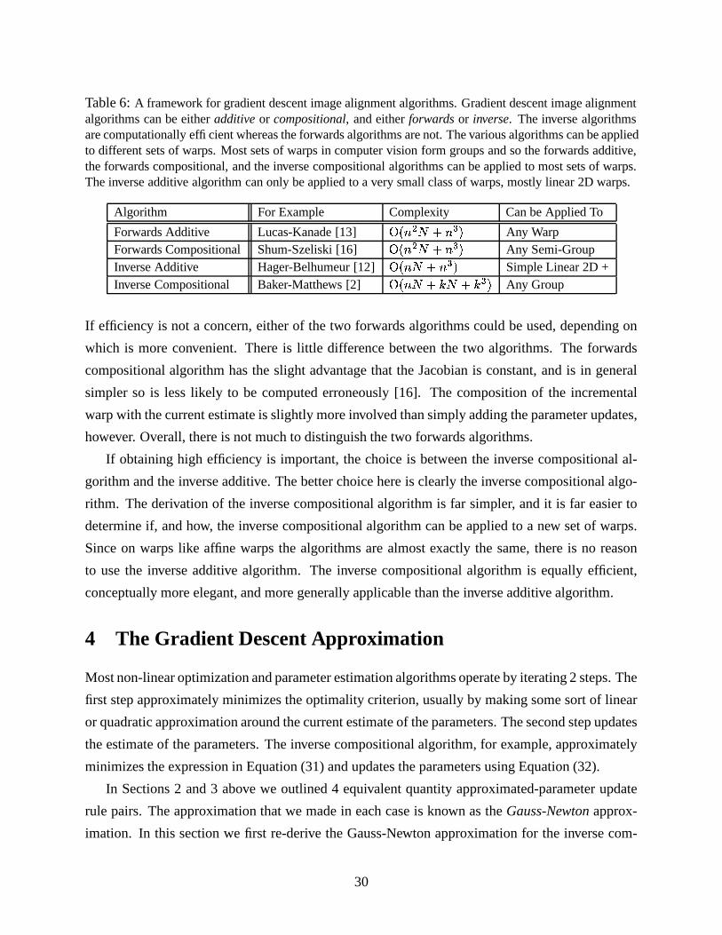
Table 6: A framework for gradient descent image alignment algorithms. Gradient descent image alignmentalgorithms can be either additive or compositional, and either forwards or inverse. The inverse algorithmsare computationally efficient whereas the forwards algorithms are not. The various algorithms can be appliedto different sets of warps. Most sets of warps in computer vision form groups and so the forwards additive,the forwards compositional, and the inverse compositional algorithms can be applied to most sets of warps.The inverse additive algorithm can only be applied to a very small class of warps, mostly linear 2D warps.

Algorithm For Example Complexity Can be Applied To

Forwards Additive Lucas-Kanade [13] � �� = � #�� L Any WarpForwards Compositional Shum-Szeliski [16] � �� = � #�� L Any Semi-GroupInverse Additive Hager-Belhumeur [12] � �� # � L Simple Linear 2D +Inverse Compositional Baker-Matthews [2] �&�� #�� #�� L Any Group

If efficiency is not a concern, either of the two forwards algorithms could be used, depending on

which is more convenient. There is little difference between the two algorithms. The forwards

compositional algorithm has the slight advantage that the Jacobian is constant, and is in general

simpler so is less likely to be computed erroneously [16]. The composition of the incremental

warp with the current estimate is slightly more involved than simply adding the parameter updates,

however. Overall, there is not much to distinguish the two forwards algorithms.

If obtaining high efficiency is important, the choice is between the inverse compositional al-

gorithm and the inverse additive. The better choice here is clearly the inverse compositional algo-

rithm. The derivation of the inverse compositional algorithm is far simpler, and it is far easier to

determine if, and how, the inverse compositional algorithm can be applied to a new set of warps.

Since on warps like affine warps the algorithms are almost exactly the same, there is no reason

to use the inverse additive algorithm. The inverse compositional algorithm is equally efficient,

conceptually more elegant, and more generally applicable than the inverse additive algorithm.

4 The Gradient Descent Approximation

Most non-linear optimization and parameter estimation algorithms operate by iterating 2 steps. The

first step approximately minimizes the optimality criterion, usually by making some sort of linear

or quadratic approximation around the current estimate of the parameters. The second step updates

the estimate of the parameters. The inverse compositional algorithm, for example, approximately

minimizes the expression in Equation (31) and updates the parameters using Equation (32).

In Sections 2 and 3 above we outlined 4 equivalent quantity approximated-parameter update

rule pairs. The approximation that we made in each case is known as the Gauss-Newton approx-

imation. In this section we first re-derive the Gauss-Newton approximation for the inverse com-

30

positional algorithm and then consider several alternative approximations. Afterwards we apply

all of the alternatives to the inverse compositional algorithm, empirically evaluating them in Sec-

tion 4.6. We conclude this section with a summary of the gradient descent options in Section 4.7

and a review of several other related algorithms in Section 4.8.

4.1 The Gauss-Newton Algorithm

The Gauss-Newton inverse compositional algorithm attempts to minimize Equation (31):]X^ _�� #" � $&�Fb = � ] ^ _ �� 3" � $4�G� a � � �!�#"%$&�%�2b =(62)

where� �!�#" � $&�# �� !�#" � $&�%�,a � � �!�#"%$&�%�

using a first order Taylor expansion of� ��#" � $&� :]�^ �� #"��C�C7 � �

� $ � $ � = � ]�^ �� !�#"��C�%�H7 �9� � � $ � $9a � � �!�#"%$&�%�� = -(63)

Here� �!�#"��C� �� !�#"��C�%�3a � � ��#"G$4�G� �8�!��#a � � �!�#"%$&�%�

,�� 9� �� , and we use

the expression�� to denote the partial derivative of

�with respect to its second vector argument� $ . The expression in Equation (63) is quadratic in � $ and has the closed form solution:

� $ a�. / * ] ^ � �

� $ � � � ��3"��C�� . / * ] ^ � � � � $ � � _ � � ��#"%$&�%�Ja�8�!��2b(64)

where.

is the first order (Gauss-Newton) approximation to the Hessian matrix:

. ] ^ � �

� $ � � � �

� $ � � ] ^ �� $ � � � � � � $ � -(65)

One simple way to see that Equations (64) and (65) are the closed-form solution to Equation (63)

is to differentiate the expression in Equation (63) with respect to � $ and set the result to zero:

� ] ^ � �

� $ � � �� !�#"��C� 7 � �

� $ � $ �` ��-(66)

Rearranging this expression gives the closed form result in Equations (64) and (65).

31

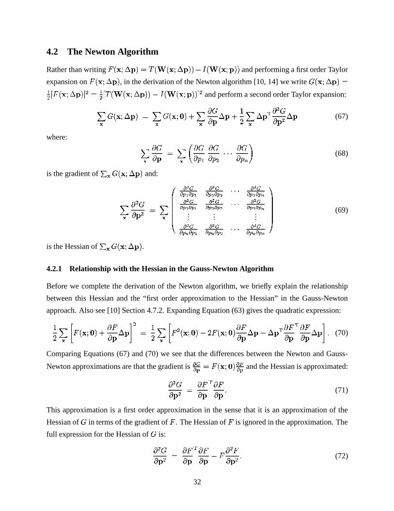
4.2 The Newton Algorithm

Rather than writing� ��#" � $&�3 �� #" � $&�%�1a � � ��3"%$4�G�

and performing a first order Taylor

expansion on� ��3" � $4� , in the derivation of the Newton algorithm [10, 14] we write � ��#" � $&�&*= _ � �!�#" � $4�Eb = *= _ �� !�#" � $&�%�Ja � � ��#"G$4�G�Fb =

and perform a second order Taylor expansion:] ^� ��3" � $4� ] ^

� ��#"��C�C7 ] ^ � �

� $ � $ 7 �� ] ^ � $ � �=�

� $ = � $ (67)

where: ]X^ � �

� $ ] ^ 6 � �

� (H* � �

� (�= IKIKI � �

� (10 > (68)

is the gradient of �^� ��#" � $&� and:

] ^ �=�

� $ = ] ^ RSSSSSST� $��#��! � �"! � $��#�"! �#� $ IKIKI � $��#��! �#��'� $��#� $ � � ! � $��#� $ �#� $ IKIKI � $��#� $ �#� '

......

...� $ �� '��#��! � $ ��#��' �#� $ IKIKI � $ �� ' � ��'UXWWWWWWY (69)

is the Hessian of �^� ��3" � $4� .

4.2.1 Relationship with the Hessian in the Gauss-Newton Algorithm

Before we complete the derivation of the Newton algorithm, we briefly explain the relationship

between this Hessian and the “first order approximation to the Hessian” in the Gauss-Newton

approach. Also see [10] Section 4.7.2. Expanding Equation (63) gives the quadratic expression:�� ] ^ �� !�#"��C� 7 � �

� $ � $ � = �� ] ^ �� = ��3"��C�C7 � � ��#"��+� � �

� $ � $ 7 � $ � � �

� $� � �

� $ � $ � - (70)

Comparing Equations (67) and (70) we see that the differences between the Newton and Gauss-

Newton approximations are that the gradient is� �� !�#"��C�"�� and the Hessian is approximated:

�=�

� $ = � �

� $� � �

� $ - (71)

This approximation is a first order approximation in the sense that it is an approximation of the

Hessian of � in terms of the gradient of�

. The Hessian of�

is ignored in the approximation. The

full expression for the Hessian of � is:

�=�

� $ = � �

� $� � �

� $ 7 � �= �

� $ = - (72)

32

4.2.2 Derivation of the Gradient and the Hessian

If � �!�#" � $&�# *= _ �� #" � $&�%��a � � �!�#"%$&�%�Fb =then the gradient is:

� �

� $ �9� � � $ � _ �� 3" � $4�G� a � � �!�#"%$&�%�2b(73)

where for convenience we use� �� to denote the partial derivative of � with respect to its second

vector argument � $ . The Hessian:

�=�

� $ = � � $ � � �= �

� � = � � � $ � _ �� 3" � $4�G�Ja � � �!�#"%$&�%�2b7�9� �

= � $ = � _ �� !�#" � $&�%�Ja � � ��#"G$4�G�2b

7 � � � � $ � � � � � � $ �(74)

where:

� �� RT � $ �� $ � $ �� $ �� $ �� $ UY (75)

is the matrix of second derivatives of the template�

and:

�9� �= � $ = �` � �� RSSSST

� $ � ��#�"! �#��! IKIKI � $ � �� "! �#��'...

...� $ � ��#� ' �#� ! IKIKI � $ � ��#� ' � � 'UXWWWWY 7 � �� RSSSST

� $ � (�#�"! �#�"! IKIKI � $ � (�#�"! � ��'...

...� $ ��(�#��' �#�"! IKIKI � $ �&(�#� ' �#� 'UXWWWWY - (76)

Equations (73) and (74) hold for arbitrary � $ . In the Newton algorithm, we just need their values

at � $ �. When � $ �

, the gradient simplifies to:

� �

� $ �9� � � $ � _ ��!��Ja � � �!�#"%$&�%�2b(77)

and the Hessian simplifies to:� $ �� $

RT � � $ � � �= �

� � = � � � $ � 7 �9� �= � $ = � UY _ �8�!��Ja � � ��#"G$4�G�Fb 7 �9� � � $ � � �9� � � $ ��-

(78)

33

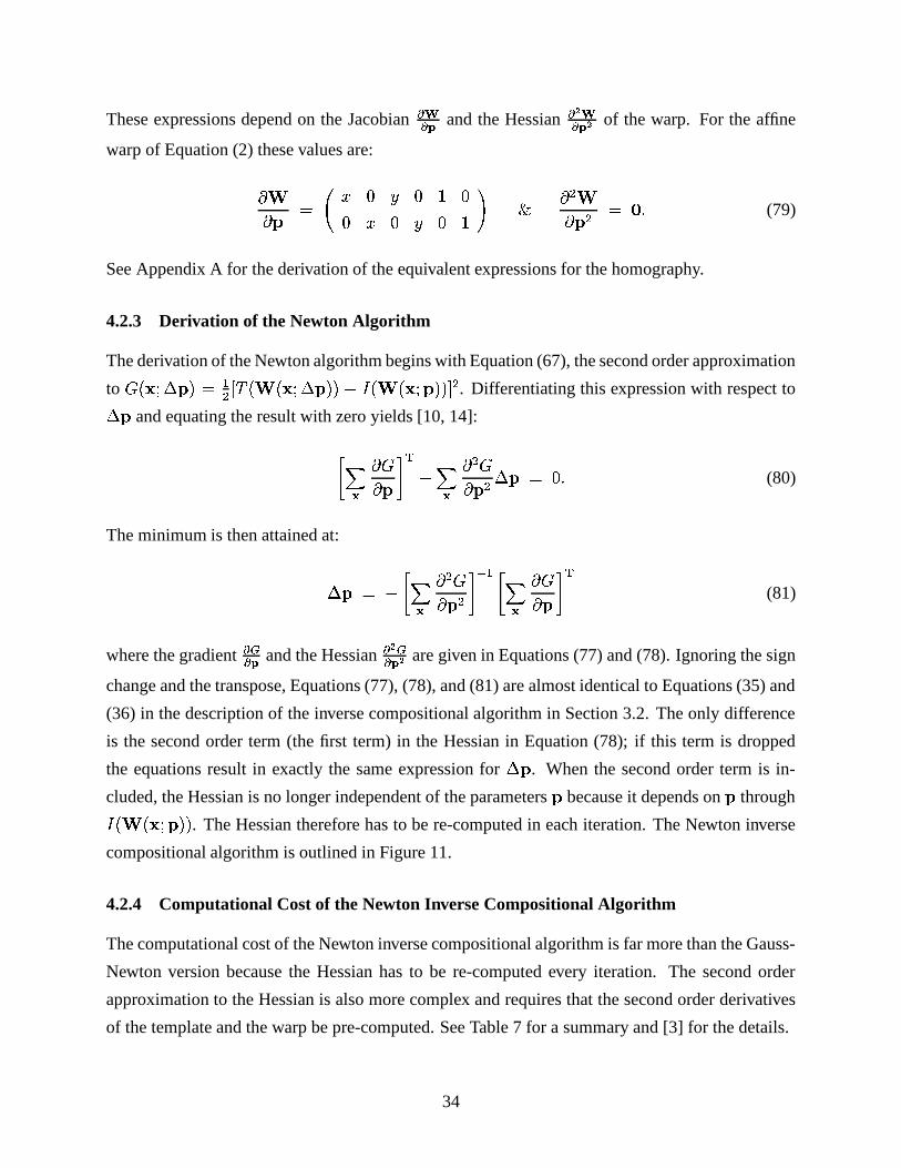
These expressions depend on the Jacobian�� and the Hessian

� $ �� $ of the warp. For the affine

warp of Equation (2) these values are:

� � $ 6 � ) � ) � )) � ) � ) � > � �= � $ = ��-

(79)

See Appendix A for the derivation of the equivalent expressions for the homography.

4.2.3 Derivation of the Newton Algorithm

The derivation of the Newton algorithm begins with Equation (67), the second order approximation

to � ��#" � $&� *= _ �8� �!�#" � $4�G�3a � � ��#"%$&�%�Eb =. Differentiating this expression with respect to� $ and equating the result with zero yields [10, 14]:

] ^ � �

� $ � � 7 ] ^ �=�

� $ = � $� ) -(80)

The minimum is then attained at:

� $� a �] ^ �=�

� $ = �/ * !] ^ � �

� $ � �(81)

where the gradient� �� and the Hessian

� $ �� $ are given in Equations (77) and (78). Ignoring the sign

change and the transpose, Equations (77), (78), and (81) are almost identical to Equations (35) and

(36) in the description of the inverse compositional algorithm in Section 3.2. The only difference

is the second order term (the first term) in the Hessian in Equation (78); if this term is dropped

the equations result in exactly the same expression for � $ . When the second order term is in-

cluded, the Hessian is no longer independent of the parameters$

because it depends on$

through� � ��#"%$&�%�. The Hessian therefore has to be re-computed in each iteration. The Newton inverse

compositional algorithm is outlined in Figure 11.

4.2.4 Computational Cost of the Newton Inverse Compositional Algorithm

The computational cost of the Newton inverse compositional algorithm is far more than the Gauss-

Newton version because the Hessian has to be re-computed every iteration. The second order

approximation to the Hessian is also more complex and requires that the second order derivatives

of the template and the warp be pre-computed. See Table 7 for a summary and [3] for the details.

34

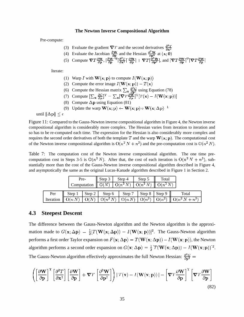
The Newton Inverse Compositional Algorithm

Pre-compute:

(3) Evaluate the gradient � � and the second derivatives� $ �� ^ $

(4) Evaluate the Jacobian�� and the Hessian

� $ �� $ at �� (5) Compute � � �� ,

� �� $ �� ^ $ � � �� #%� � � � $ �� $ � , and

��

Iterate:

(1) Warp � with �� to compute ��(2) Compute the error image �� (6) Compute the Hessian matrix �

^ � $�� $ using Equation (78)

(7) Compute

��^ � �� ^ � ��

(8) Compute �&� using Equation (81)(9) Update the warp �� &�� / *

until '(�� '+* ,Figure 11: Compared to the Gauss-Newton inverse compositional algorithm in Figure 4, the Newton inversecompositional algorithm is considerably more complex. The Hessian varies from iteration to iteration andso has to be re-computed each time. The expression for the Hessian is also considerably more complex andrequires the second order derivatives of both the template � and the warp �� . The computational costof the Newton inverse compositional algorithm is � �� = � # � L and the pre-computation cost is � �� = � .Table 7: The computation cost of the Newton inverse compositional algorithm. The one time pre-computation cost in Steps 3-5 is � �� = � . After that, the cost of each iteration is � �� = � # � L , sub-stantially more than the cost of the Gauss-Newton inverse compositional algorithm described in Figure 4,and asymptotically the same as the original Lucas-Kanade algorithm described in Figure 1 in Section 2.

Pre- Step 3 Step 4 Step 5 TotalComputation � � � � �� = � � �� = � � �� = �

Per Step 1 Step 2 Step 6 Step 7 Step 8 Step 9 TotalIteration � �� = � � �� L � �� = � �� = � # � L

4.3 Steepest Descent

The difference between the Gauss-Newton algorithm and the Newton algorithm is the approxi-

mation made to � ��#" � $&� *= _ �� !�#" � $&�%� a � � �!�#"%$&�%�Eb =. The Gauss-Newton algorithm

performs a first order Taylor expansion on� �!�#" � $&�� !�#" � $&�%� a � � ��3"%$4�G�

, the Newton

algorithm performs a second order expansion on � �!�#" � $4� *= _ �� #" � $&�%��a � � ��#"G$4�G�Fb =.

The Gauss-Newton algorithm effectively approximates the full Newton Hessian:� $ �� $

RT � � $ � � �= �

� � = � � � $ � 7 �9� �= � $ = � UY _ ��Ja � � �!�#"%$&�%�2b 7 � � � � $ � � �� $ �

(82)

35

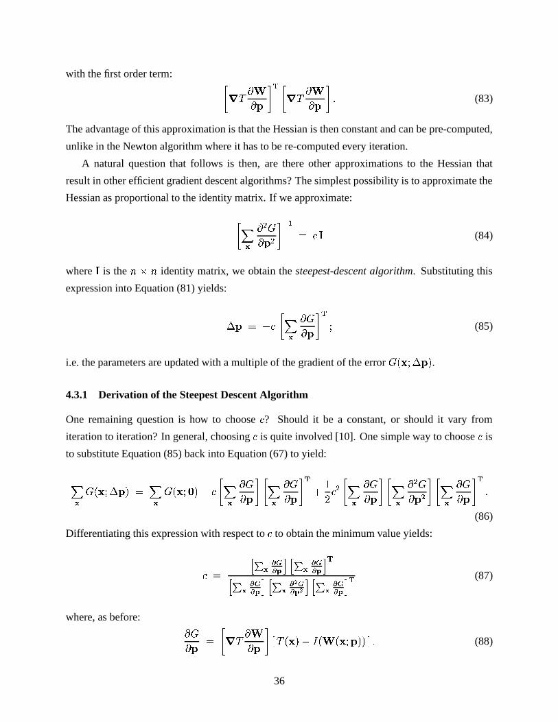
with the first order term: � � � � $ � � �� $ ��-(83)

The advantage of this approximation is that the Hessian is then constant and can be pre-computed,

unlike in the Newton algorithm where it has to be re-computed every iteration.

A natural question that follows is then, are there other approximations to the Hessian that

result in other efficient gradient descent algorithms? The simplest possibility is to approximate the

Hessian as proportional to the identity matrix. If we approximate:

] ^ �=�

� $ = �/ * ��

(84)

where�

is the \ � \ identity matrix, we obtain the steepest-descent algorithm. Substituting this

expression into Equation (81) yields:

� $ a�� ] ^ � �

� $ � � "(85)

i.e. the parameters are updated with a multiple of the gradient of the error � ��#" � $&� .4.3.1 Derivation of the Steepest Descent Algorithm

One remaining question is how to choose�? Should it be a constant, or should it vary from

iteration to iteration? In general, choosing�

is quite involved [10]. One simple way to choose�

is

to substitute Equation (85) back into Equation (67) to yield:]�^� �!�#" � $&�< ]�^

� ��3"��C�Ja�� !]X^ � �

� $ � ]X^ � �

� $ � � 7 �� = ]�^ � �

� $ � �]X^ �=�

� $ = � !]X^ � �

� $ � � -(86)

Differentiating this expression with respect to�

to obtain the minimum value yields:

�Z � � ^ � �� ^ � �� ^ � �� ^ � $ �� $ � � � ^ � �� (87)

where, as before:

� �

� $ �� $ � _ ��Ja � � ��#"G$4�G�2b -(88)

36

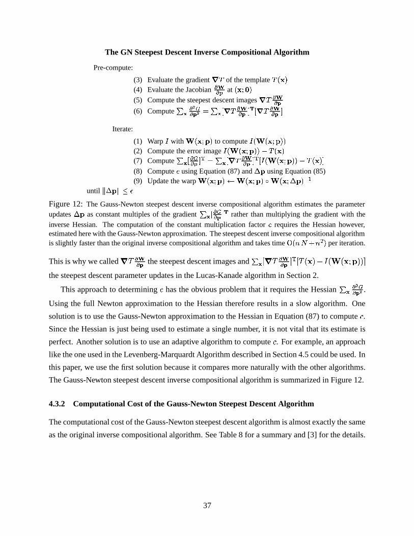
The GN Steepest Descent Inverse Compositional Algorithm

Pre-compute:

(3) Evaluate the gradient �� of the template ��(4) Evaluate the Jacobian

�� at �� (5) Compute the steepest descent images �� (6) Compute �

^ � $�� $ � � ^ � � � �� Iterate:

(1) Warp � with �� to compute ��(2) Compute the error image �� (7) Compute �

^ � � �� ^ � � � �� (8) Compute � using Equation (87) and �&� using Equation (85)(9) Update the warp �� "�� / *

until '(�&�)'+*%,Figure 12: The Gauss-Newton steepest descent inverse compositional algorithm estimates the parameterupdates �&� as constant multiples of the gradient �

^ � � �� rather than multiplying the gradient with the

inverse Hessian. The computation of the constant multiplication factor � requires the Hessian however,estimated here with the Gauss-Newton approximation. The steepest descent inverse compositional algorithmis slightly faster than the original inverse compositional algorithm and takes time � �� # � = per iteration.

This is why we called�� the steepest descent images and �

^ _ �9� �� b � _ �� a � � �!�#"%$&�%�Fbthe steepest descent parameter updates in the Lucas-Kanade algorithm in Section 2.

This approach to determining�

has the obvious problem that it requires the Hessian �^ � $ �� $ .

Using the full Newton approximation to the Hessian therefore results in a slow algorithm. One

solution is to use the Gauss-Newton approximation to the Hessian in Equation (87) to compute�.

Since the Hessian is just being used to estimate a single number, it is not vital that its estimate is

perfect. Another solution is to use an adaptive algorithm to compute�. For example, an approach

like the one used in the Levenberg-Marquardt Algorithm described in Section 4.5 could be used. In

this paper, we use the first solution because it compares more naturally with the other algorithms.

The Gauss-Newton steepest descent inverse compositional algorithm is summarized in Figure 12.

4.3.2 Computational Cost of the Gauss-Newton Steepest Descent Algorithm

The computational cost of the Gauss-Newton steepest descent algorithm is almost exactly the same

as the original inverse compositional algorithm. See Table 8 for a summary and [3] for the details.

37

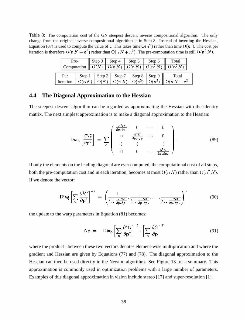
Table 8: The computation cost of the GN steepest descent inverse compositional algorithm. The onlychange from the original inverse compositional algorithm is in Step 8. Instead of inverting the Hessian,Equation (87) is used to compute the value of � . This takes time �&�� = rather than time � �� L . The cost periteration is therefore � �� #�� = rather than � �� #�� L . The pre-computation time is still � �� = � .

Pre- Step 3 Step 4 Step 5 Step 6 TotalComputation �&� � � �� = � �&�� = �

Per Step 1 Step 2 Step 7 Step 8 Step 9 TotalIteration � �� &� � � �� = � �� = � �� #�� =

4.4 The Diagonal Approximation to the Hessian

The steepest descent algorithm can be regarded as approximating the Hessian with the identity

matrix. The next simplest approximation is to make a diagonal approximation to the Hessian:

�� =�

� $ = �` ] ^ RSSSSSST� $��#��! �#�"! ) IKIKI )) � $�� $ �#� $ IKIKI )

......

...) ) IKIKI � $ ��#� ' �#� 'UXWWWWWWY - (89)

If only the elements on the leading diagonal are ever computed, the computational cost of all steps,

both the pre-computation cost and in each iteration, becomes at most � � \�� rather than � � \ = � � .If we denote the vector:

�� ] ^ �=�

� $ = �/ * RT �

�^ � $ ��#�"! �#�"! � �

�^ � $ ��#�%$ � � $ �/-.-.-/� �

�^ � $ ��#��'�� ' UY � (90)

the update to the warp parameters in Equation (81) becomes:

� $� a�� !] ^ �=�

� $ = �/ * I !] ^ � �

� $ � �(91)

where the productIbetween these two vectors denotes element-wise multiplication and where the

gradient and Hessian are given by Equations (77) and (78). The diagonal approximation to the

Hessian can then be used directly in the Newton algorithm. See Figure 13 for a summary. This

approximation is commonly used in optimization problems with a large number of parameters.

Examples of this diagonal approximation in vision include stereo [17] and super-resolution [1].

38

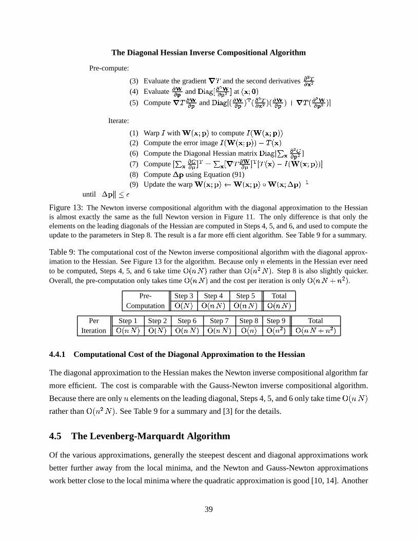
The Diagonal Hessian Inverse Compositional Algorithm

Pre-compute:

(3) Evaluate the gradient � � and the second derivatives� $ �� ^ $

(4) Evaluate�� and ��

� � $ �� $ � at �� (5) Compute � � �� and ��

�� $ �� ^ $ � �� # �� $ �� $ �

Iterate:

(1) Warp � with �� to compute ��(2) Compute the error image �� (6) Compute the Diagonal Hessian matrix ��

��^ � $�� $ ]

(7) Compute

��^ � �� ^ � � � ��

(8) Compute �&� using Equation (91)(9) Update the warp �� &� / *

until '(�&�)'+*-,Figure 13: The Newton inverse compositional algorithm with the diagonal approximation to the Hessianis almost exactly the same as the full Newton version in Figure 11. The only difference is that only theelements on the leading diagonals of the Hessian are computed in Steps 4, 5, and 6, and used to compute theupdate to the parameters in Step 8. The result is a far more efficient algorithm. See Table 9 for a summary.

Table 9: The computational cost of the Newton inverse compositional algorithm with the diagonal approx-imation to the Hessian. See Figure 13 for the algorithm. Because only � elements in the Hessian ever needto be computed, Steps 4, 5, and 6 take time � �� rather than �&�� = � . Step 8 is also slightly quicker.Overall, the pre-computation only takes time � �� and the cost per iteration is only � �� # � = .

Pre- Step 3 Step 4 Step 5 TotalComputation � � � � ��

Per Step 1 Step 2 Step 6 Step 7 Step 8 Step 9 TotalIteration �&�� &�� = � �� # � =

4.4.1 Computational Cost of the Diagonal Approximation to the Hessian

The diagonal approximation to the Hessian makes the Newton inverse compositional algorithm far

more efficient. The cost is comparable with the Gauss-Newton inverse compositional algorithm.

Because there are only \ elements on the leading diagonal, Steps 4, 5, and 6 only take time � � \�� rather than � � \ = � � . See Table 9 for a summary and [3] for the details.

4.5 The Levenberg-Marquardt Algorithm

Of the various approximations, generally the steepest descent and diagonal approximations work

better further away from the local minima, and the Newton and Gauss-Newton approximations

work better close to the local minima where the quadratic approximation is good [10, 14]. Another

39

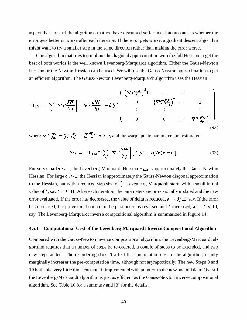
aspect that none of the algorithms that we have discussed so far take into account is whether the

error gets better or worse after each iteration. If the error gets worse, a gradient descent algorithm

might want to try a smaller step in the same direction rather than making the error worse.

One algorithm that tries to combine the diagonal approximation with the full Hessian to get the

best of both worlds is the well known Levenberg-Marquardt algorithm. Either the Gauss-Newton

Hessian or the Newton Hessian can be used. We will use the Gauss-Newton approximation to get

an efficient algorithm. The Gauss-Newton Levenberg-Marquardt algorithm uses the Hessian:

�� ] ^ � � � � $ � � � � � � $ � 7�� ] ^ RSSSSSSSST� �9� ��#��! � = ) IKIKI )

) � �� #� $ � = IKIKI )...

......) ) IKIKI � � � ��#��' � =

UXWWWWWWWWY(92)

where� � ��#�� #�� 7 � �� (�#�� ,

��

), and the warp update parameters are estimated:

� $� a�� / * ] ^ �� $ � _ �8�!�� a � � ��#"G$4�G�2b -(93)

For very small��

, the Levenberg-Marquardt Hessian��

is approximately the Gauss-Newton

Hessian. For large��

, the Hessian is approximately the Gauss-Newton diagonal approximation

to the Hessian, but with a reduced step size of*� . Levenberg-Marquardt starts with a small initial

value of�, say

� ) - ) �. After each iteration, the parameters are provisionally updated and the new

error evaluated. If the error has decreased, the value of delta is reduced,�� ")

, say. If the error

has increased, the provisional update to the parameters is reversed and�

increased,�� ") ,

say. The Levenberg-Marquardt inverse compositional algorithm is summarized in Figure 14.

4.5.1 Computational Cost of the Levenberg-Marquardt Inverse Compositional Algorithm

Compared with the Gauss-Newton inverse compositional algorithm, the Levenberg-Marquardt al-

gorithm requires that a number of steps be re-ordered, a couple of steps to be extended, and two

new steps added. The re-ordering doesn’t affect the computation cost of the algorithm; it only

marginally increases the pre-computation time, although not asymptotically. The new Steps 0 and

10 both take very little time, constant if implemented with pointers to the new and old data. Overall

the Levenberg-Marquardt algorithm is just as efficient as the Gauss-Newton inverse compositional

algorithm. See Table 10 for a summary and [3] for the details.

40

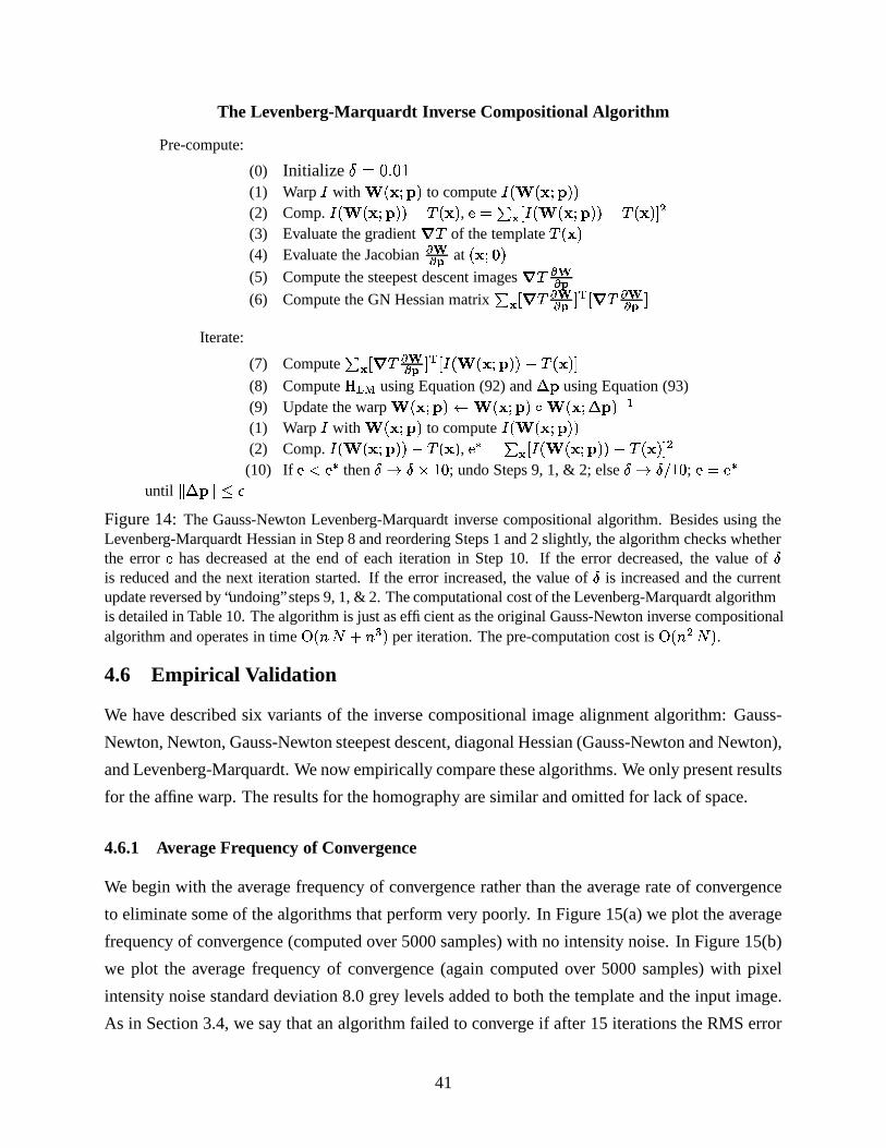
The Levenberg-Marquardt Inverse Compositional Algorithm

Pre-compute:

(0) Initialize� ) - ) �

(1) Warp � with �� to compute �� (2) Comp. �� , � � �

^ �� =

(3) Evaluate the gradient � � of the template ��(4) Evaluate the Jacobian

�� at �� (5) Compute the steepest descent images � � ��(6) Compute the GN Hessian matrix �

^��

Iterate:

(7) Compute �^��

(8) Compute� ��

using Equation (92) and �&� using Equation (93)(9) Update the warp �� &�� / *(1) Warp � with �� to compute �� (2) Comp. �� , � � � �

^ �� =

(10) If ��

then �� ; undo Steps 9, 1, & 2; else �� ; � ��

until '(�&�)'+*-,Figure 14: The Gauss-Newton Levenberg-Marquardt inverse compositional algorithm. Besides using theLevenberg-Marquardt Hessian in Step 8 and reordering Steps 1 and 2 slightly, the algorithm checks whetherthe error � has decreased at the end of each iteration in Step 10. If the error decreased, the value of �is reduced and the next iteration started. If the error increased, the value of � is increased and the currentupdate reversed by “undoing” steps 9, 1, & 2. The computational cost of the Levenberg-Marquardt algorithmis detailed in Table 10. The algorithm is just as efficient as the original Gauss-Newton inverse compositionalalgorithm and operates in time � �� #�� L per iteration. The pre-computation cost is � �� = � .4.6 Empirical Validation

We have described six variants of the inverse compositional image alignment algorithm: Gauss-

Newton, Newton, Gauss-Newton steepest descent, diagonal Hessian (Gauss-Newton and Newton),

and Levenberg-Marquardt. We now empirically compare these algorithms. We only present results

for the affine warp. The results for the homography are similar and omitted for lack of space.

4.6.1 Average Frequency of Convergence

We begin with the average frequency of convergence rather than the average rate of convergence

to eliminate some of the algorithms that perform very poorly. In Figure 15(a) we plot the average

frequency of convergence (computed over 5000 samples) with no intensity noise. In Figure 15(b)

we plot the average frequency of convergence (again computed over 5000 samples) with pixel

intensity noise standard deviation 8.0 grey levels added to both the template and the input image.

As in Section 3.4, we say that an algorithm failed to converge if after 15 iterations the RMS error

41

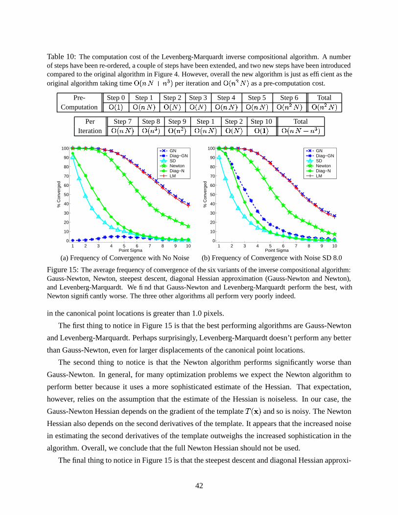
Table 10: The computation cost of the Levenberg-Marquardt inverse compositional algorithm. A numberof steps have been re-ordered, a couple of steps have been extended, and two new steps have been introducedcompared to the original algorithm in Figure 4. However, overall the new algorithm is just as efficient as theoriginal algorithm taking time � �� #�� L per iteration and � �� = � as a pre-computation cost.

Pre- Step 0 Step 1 Step 2 Step 3 Step 4 Step 5 Step 6 TotalComputation � � � � �� = � � �� = �

Per Step 7 Step 8 Step 9 Step 1 Step 2 Step 10 TotalIteration � �� &�� L �&�� = �&�� &�� #�� L

1 2 3 4 5 6 7 8 9 100

10

20

30

40

50

60

70

80

90

100

Point Sigma

% C

onve

rged

GNDiag−GNSDNewtonDiag−NLM

1 2 3 4 5 6 7 8 9 100

10

20

30

40

50

60

70

80

90

100

Point Sigma

% C

onve

rged

GNDiag−GNSDNewtonDiag−NLM

(a) Frequency of Convergence with No Noise (b) Frequency of Convergence with Noise SD 8.0

Figure 15: The average frequency of convergence of the six variants of the inverse compositional algorithm:Gauss-Newton, Newton, steepest descent, diagonal Hessian approximation (Gauss-Newton and Newton),and Levenberg-Marquardt. We find that Gauss-Newton and Levenberg-Marquardt perform the best, withNewton significantly worse. The three other algorithms all perform very poorly indeed.

in the canonical point locations is greater than 1.0 pixels.

The first thing to notice in Figure 15 is that the best performing algorithms are Gauss-Newton

and Levenberg-Marquardt. Perhaps surprisingly, Levenberg-Marquardt doesn’t perform any better

than Gauss-Newton, even for larger displacements of the canonical point locations.

The second thing to notice is that the Newton algorithm performs significantly worse than

Gauss-Newton. In general, for many optimization problems we expect the Newton algorithm to

perform better because it uses a more sophisticated estimate of the Hessian. That expectation,

however, relies on the assumption that the estimate of the Hessian is noiseless. In our case, the

Gauss-Newton Hessian depends on the gradient of the template��

and so is noisy. The Newton

Hessian also depends on the second derivatives of the template. It appears that the increased noise

in estimating the second derivatives of the template outweighs the increased sophistication in the

algorithm. Overall, we conclude that the full Newton Hessian should not be used.

The final thing to notice in Figure 15 is that the steepest descent and diagonal Hessian approxi-

42

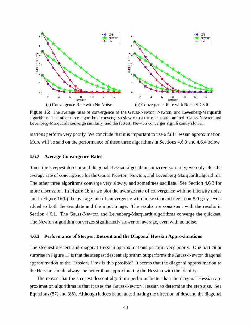
2 4 6 8 10 12 14

0

1

2

3

4

5

6

Iteration

RM

S P

oint

Err

orGNNewtonLM

2 4 6 8 10 12 14

0

1

2

3

4

5

6

Iteration

RM

S P

oint

Err

or

GNNewtonLM

(a) Convergence Rate with No Noise (b) Convergence Rate with Noise SD 8.0

Figure 16: The average rates of convergence of the Gauss-Newton, Newton, and Levenberg-Marquardtalgorithms. The other three algorithms converge so slowly that the results are omitted. Gauss-Newton andLevenberg-Marquardt converge similarly, and the fastest. Newton converges significantly slower.

mations perform very poorly. We conclude that it is important to use a full Hessian approximation.

More will be said on the performance of these three algorithms in Sections 4.6.3 and 4.6.4 below.

4.6.2 Average Convergence Rates

Since the steepest descent and diagonal Hessian algorithms converge so rarely, we only plot the

average rate of convergence for the Gauss-Newton, Newton, and Levenberg-Marquardt algorithms.

The other three algorithms converge very slowly, and sometimes oscillate. See Section 4.6.3 for

more discussion. In Figure 16(a) we plot the average rate of convergence with no intensity noise

and in Figure 16(b) the average rate of convergence with noise standard deviation 8.0 grey levels

added to both the template and the input image. The results are consistent with the results in

Section 4.6.1. The Gauss-Newton and Levenberg-Marquardt algorithms converge the quickest.

The Newton algorithm converges significantly slower on average, even with no noise.

4.6.3 Performance of Steepest Descent and the Diagonal Hessian Approximations

The steepest descent and diagonal Hessian approximations perform very poorly. One particular

surprise in Figure 15 is that the steepest descent algorithm outperforms the Gauss-Newton diagonal

approximation to the Hessian. How is this possible? It seems that the diagonal approximation to

the Hessian should always be better than approximating the Hessian with the identity.

The reason that the steepest descent algorithm performs better than the diagonal Hessian ap-

proximation algorithms is that it uses the Gauss-Newton Hessian to determine the step size. See

Equations (87) and (88). Although it does better at estimating the direction of descent, the diagonal

43

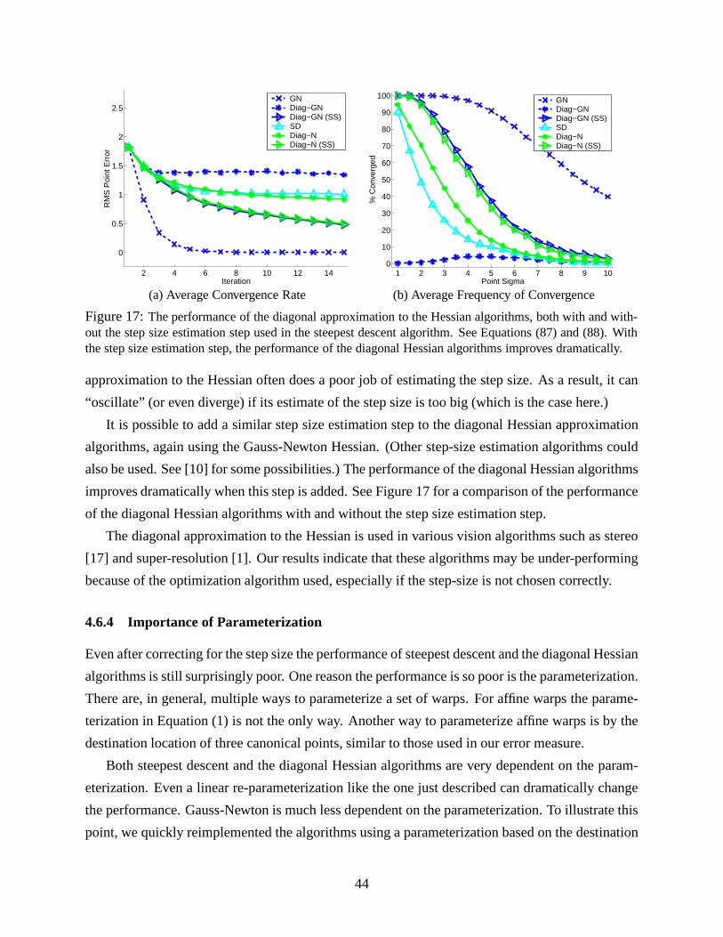
2 4 6 8 10 12 14

0

0.5

1

1.5

2

2.5

Iteration

RM

S P

oint

Err

orGNDiag−GNDiag−GN (SS)SDDiag−NDiag−N (SS)

1 2 3 4 5 6 7 8 9 100

10

20

30

40

50

60

70

80

90

100

Point Sigma

% C

onve

rged

GNDiag−GNDiag−GN (SS)SDDiag−NDiag−N (SS)

(a) Average Convergence Rate (b) Average Frequency of Convergence

Figure 17: The performance of the diagonal approximation to the Hessian algorithms, both with and with-out the step size estimation step used in the steepest descent algorithm. See Equations (87) and (88). Withthe step size estimation step, the performance of the diagonal Hessian algorithms improves dramatically.

approximation to the Hessian often does a poor job of estimating the step size. As a result, it can

“oscillate” (or even diverge) if its estimate of the step size is too big (which is the case here.)

It is possible to add a similar step size estimation step to the diagonal Hessian approximation

algorithms, again using the Gauss-Newton Hessian. (Other step-size estimation algorithms could

also be used. See [10] for some possibilities.) The performance of the diagonal Hessian algorithms

improves dramatically when this step is added. See Figure 17 for a comparison of the performance

of the diagonal Hessian algorithms with and without the step size estimation step.

The diagonal approximation to the Hessian is used in various vision algorithms such as stereo

[17] and super-resolution [1]. Our results indicate that these algorithms may be under-performing

because of the optimization algorithm used, especially if the step-size is not chosen correctly.

4.6.4 Importance of Parameterization

Even after correcting for the step size the performance of steepest descent and the diagonal Hessian

algorithms is still surprisingly poor. One reason the performance is so poor is the parameterization.

There are, in general, multiple ways to parameterize a set of warps. For affine warps the parame-

terization in Equation (1) is not the only way. Another way to parameterize affine warps is by the

destination location of three canonical points, similar to those used in our error measure.

Both steepest descent and the diagonal Hessian algorithms are very dependent on the param-

eterization. Even a linear re-parameterization like the one just described can dramatically change

the performance. Gauss-Newton is much less dependent on the parameterization. To illustrate this

point, we quickly reimplemented the algorithms using a parameterization based on the destination

44

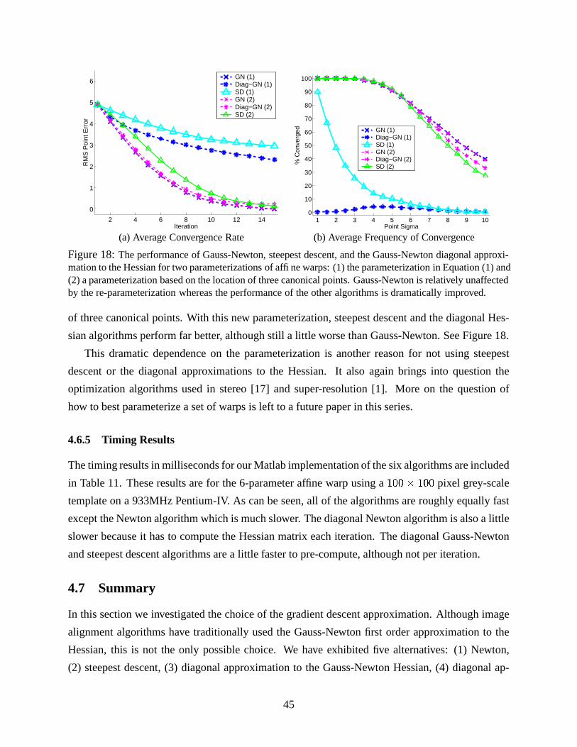
2 4 6 8 10 12 14

0

1

2

3

4

5

6

Iteration

RM

S P

oint

Err

orGN (1)Diag−GN (1)SD (1)GN (2)Diag−GN (2)SD (2)

1 2 3 4 5 6 7 8 9 100

10

20

30

40

50

60

70

80

90

100

Point Sigma

% C

onve

rged GN (1)

Diag−GN (1)SD (1)GN (2)Diag−GN (2)SD (2)

(a) Average Convergence Rate (b) Average Frequency of Convergence

Figure 18: The performance of Gauss-Newton, steepest descent, and the Gauss-Newton diagonal approxi-mation to the Hessian for two parameterizations of affine warps: (1) the parameterization in Equation (1) and(2) a parameterization based on the location of three canonical points. Gauss-Newton is relatively unaffectedby the re-parameterization whereas the performance of the other algorithms is dramatically improved.

of three canonical points. With this new parameterization, steepest descent and the diagonal Hes-

sian algorithms perform far better, although still a little worse than Gauss-Newton. See Figure 18.

This dramatic dependence on the parameterization is another reason for not using steepest

descent or the diagonal approximations to the Hessian. It also again brings into question the

optimization algorithms used in stereo [17] and super-resolution [1]. More on the question of

how to best parameterize a set of warps is left to a future paper in this series.

4.6.5 Timing Results

The timing results in milliseconds for our Matlab implementation of the six algorithms are included

in Table 11. These results are for the 6-parameter affine warp using a �� pixel grey-scale

template on a 933MHz Pentium-IV. As can be seen, all of the algorithms are roughly equally fast

except the Newton algorithm which is much slower. The diagonal Newton algorithm is also a little

slower because it has to compute the Hessian matrix each iteration. The diagonal Gauss-Newton

and steepest descent algorithms are a little faster to pre-compute, although not per iteration.

4.7 Summary

In this section we investigated the choice of the gradient descent approximation. Although image

alignment algorithms have traditionally used the Gauss-Newton first order approximation to the

Hessian, this is not the only possible choice. We have exhibited five alternatives: (1) Newton,

(2) steepest descent, (3) diagonal approximation to the Gauss-Newton Hessian, (4) diagonal ap-

45

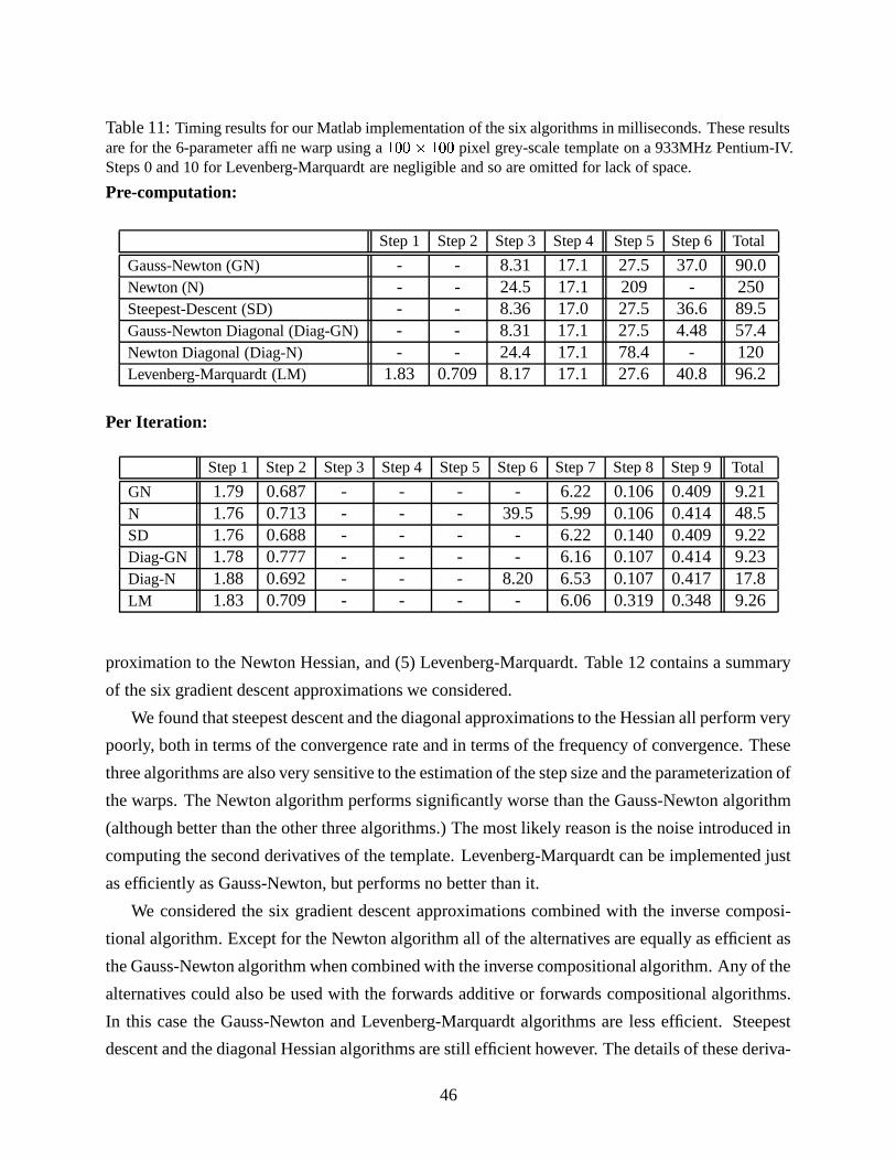
Table 11: Timing results for our Matlab implementation of the six algorithms in milliseconds. These resultsare for the 6-parameter affine warp using a

�� pixel grey-scale template on a 933MHz Pentium-IV.

Steps 0 and 10 for Levenberg-Marquardt are negligible and so are omitted for lack of space.

Pre-computation:

Step 1 Step 2 Step 3 Step 4 Step 5 Step 6 Total

Gauss-Newton (GN) - - 8.31 17.1 27.5 37.0 90.0Newton (N) - - 24.5 17.1 209 - 250Steepest-Descent (SD) - - 8.36 17.0 27.5 36.6 89.5Gauss-Newton Diagonal (Diag-GN) - - 8.31 17.1 27.5 4.48 57.4Newton Diagonal (Diag-N) - - 24.4 17.1 78.4 - 120Levenberg-Marquardt (LM) 1.83 0.709 8.17 17.1 27.6 40.8 96.2

Per Iteration:

Step 1 Step 2 Step 3 Step 4 Step 5 Step 6 Step 7 Step 8 Step 9 Total

GN 1.79 0.687 - - - - 6.22 0.106 0.409 9.21N 1.76 0.713 - - - 39.5 5.99 0.106 0.414 48.5SD 1.76 0.688 - - - - 6.22 0.140 0.409 9.22Diag-GN 1.78 0.777 - - - - 6.16 0.107 0.414 9.23Diag-N 1.88 0.692 - - - 8.20 6.53 0.107 0.417 17.8LM 1.83 0.709 - - - - 6.06 0.319 0.348 9.26

proximation to the Newton Hessian, and (5) Levenberg-Marquardt. Table 12 contains a summary

of the six gradient descent approximations we considered.

We found that steepest descent and the diagonal approximations to the Hessian all perform very

poorly, both in terms of the convergence rate and in terms of the frequency of convergence. These

three algorithms are also very sensitive to the estimation of the step size and the parameterization of

the warps. The Newton algorithm performs significantly worse than the Gauss-Newton algorithm

(although better than the other three algorithms.) The most likely reason is the noise introduced in

computing the second derivatives of the template. Levenberg-Marquardt can be implemented just

as efficiently as Gauss-Newton, but performs no better than it.

We considered the six gradient descent approximations combined with the inverse composi-

tional algorithm. Except for the Newton algorithm all of the alternatives are equally as efficient as

the Gauss-Newton algorithm when combined with the inverse compositional algorithm. Any of the

alternatives could also be used with the forwards additive or forwards compositional algorithms.

In this case the Gauss-Newton and Levenberg-Marquardt algorithms are less efficient. Steepest

descent and the diagonal Hessian algorithms are still efficient however. The details of these deriva-

46

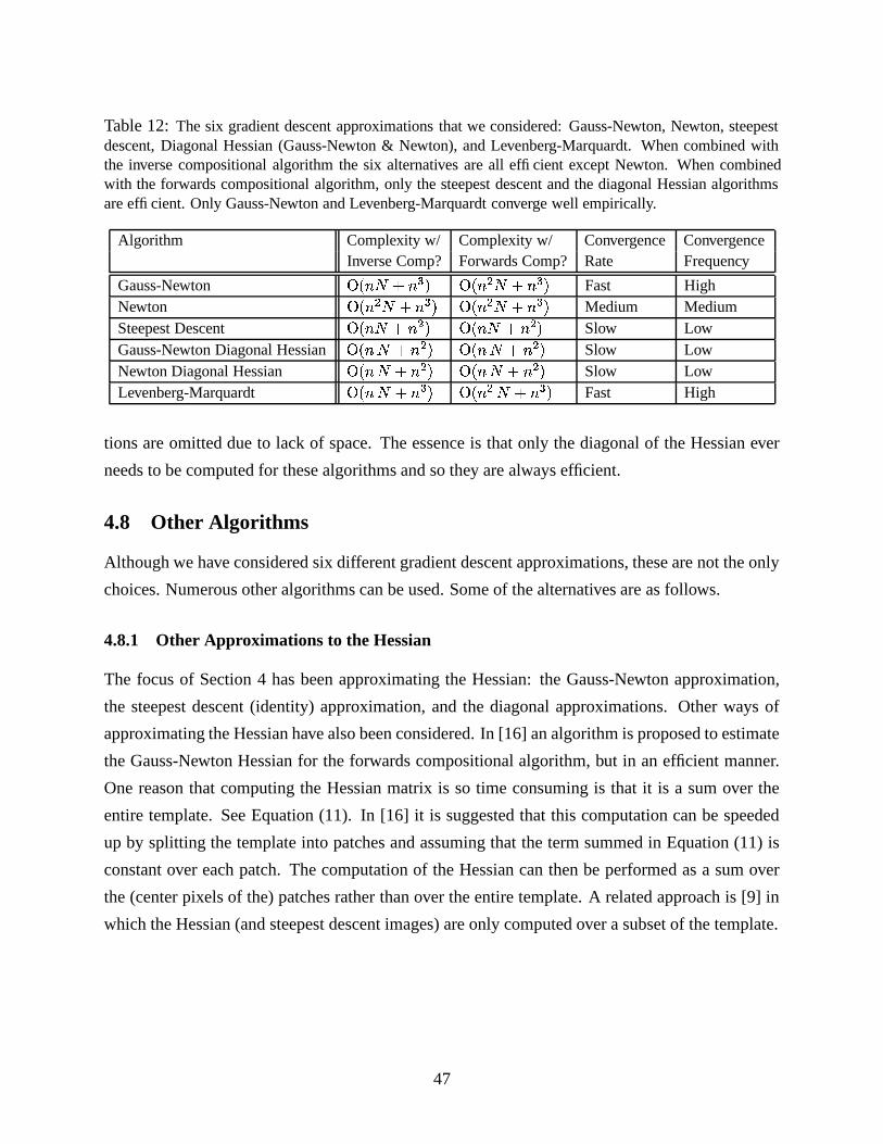
Table 12: The six gradient descent approximations that we considered: Gauss-Newton, Newton, steepestdescent, Diagonal Hessian (Gauss-Newton & Newton), and Levenberg-Marquardt. When combined withthe inverse compositional algorithm the six alternatives are all efficient except Newton. When combinedwith the forwards compositional algorithm, only the steepest descent and the diagonal Hessian algorithmsare efficient. Only Gauss-Newton and Levenberg-Marquardt converge well empirically.

Algorithm Complexity w/ Complexity w/ Convergence ConvergenceInverse Comp? Forwards Comp? Rate Frequency

Gauss-Newton � �� # � L � �� = � # � L Fast HighNewton � �� = � #�� L � �� = � # � L Medium MediumSteepest Descent � �� # � = � �� # � = Slow LowGauss-Newton Diagonal Hessian � �� #�� = � �� # � = Slow LowNewton Diagonal Hessian � �� #�� = � �� # � = Slow LowLevenberg-Marquardt � �� #�� L � �� = � # � L Fast High

tions are omitted due to lack of space. The essence is that only the diagonal of the Hessian ever

needs to be computed for these algorithms and so they are always efficient.

4.8 Other Algorithms

Although we have considered six different gradient descent approximations, these are not the only

choices. Numerous other algorithms can be used. Some of the alternatives are as follows.

4.8.1 Other Approximations to the Hessian

The focus of Section 4 has been approximating the Hessian: the Gauss-Newton approximation,

the steepest descent (identity) approximation, and the diagonal approximations. Other ways of

approximating the Hessian have also been considered. In [16] an algorithm is proposed to estimate

the Gauss-Newton Hessian for the forwards compositional algorithm, but in an efficient manner.

One reason that computing the Hessian matrix is so time consuming is that it is a sum over the

entire template. See Equation (11). In [16] it is suggested that this computation can be speeded

up by splitting the template into patches and assuming that the term summed in Equation (11) is

constant over each patch. The computation of the Hessian can then be performed as a sum over

the (center pixels of the) patches rather than over the entire template. A related approach is [9] in

which the Hessian (and steepest descent images) are only computed over a subset of the template.

47

4.8.2 Non Gradient Descent Algorithms

The essence of the gradient descent approximation is to find a linear relationship between the in-

crements to the parameters and the error image. See Equation (10). In the inverse compositional

algorithm, we analytically derived an algorithm in which this linear relationship has constant coef-

ficient. Since the coefficients are constant they can be pre-computed. Other approaches consist of

assuming that linear relationship is constant and: (1) using linear regression to find the coefficients

[8] and (2) numerically estimating the coefficients using a “difference decomposition” [11, 15, 6].

5 Discussion

We have described a unifying framework for image alignment consisting of two halves. In the first

half we classified algorithms by the quantity approximated and the warp update rule. Algorithms

can be classified as either additive or compositional and as either forwards or inverse. In the second

half we considered the gradient descent approximation. We considered the Gauss-Newton approx-

imation, the Newton approximation, the steepest descent approximation, two diagonal Hessian

approximations, and the Levenberg-Marquardt approximation. These two choices are orthogonal.

For example, one could derive a forwards compositional steepest descent algorithm.

The results of the first half are summarized in Table 6. All four algorithms empirically perform

equivalently. The only differences between the algorithms are their computational complexity and

the set of warps they can be applied to. The results of the second half are summarized in Table 12.

The algorithms differ in both their computational complexity and their empirical performance.

Overall the choice of which algorithm to use depends on two main things: (1) whether there

is likely to me more noise in the template or in the input image and (2) whether the algorithm

needs to be efficient or not. If there is more noise in the template a forwards algorithm should

be used. If there is more noise in the input image an inverse algorithm should be used. If an

efficient algorithm is required, the best options are the inverse compositional Gauss-Newton and

the inverse compositional Levenberg-Marquardt algorithms. The diagonal Hessian and steepest

descent forwards algorithms are another option, but given their poor convergence properties it is

probably better to use the inverse compositional algorithm even if the template is noisy.

Besides the choices we have described in this paper, there are several other ones that can be

made by an image alignment algorithm. These include the choice of the error norm, whether to

allow illumination or more general appearance variation, whether to add priors on the parameters,

and whether to use techniques to try to avoid local minima. In future papers in this series we will

extend our framework to cover these choices and, in particular, investigate whether the inverse

48

compositional algorithm is compatible with these extensions of the Lucas-Kanade algorithm.

6 Matlab Code, Test Images, and Scripts

Matlab implementations of all of the algorithms described in this paper are available on the World

Wide Web at: http://www.cs.cmu.edu/˜iainm/lk20. We have also included all of the test images

and the scripts used to generate the experimental results in this paper.

Acknowledgments

We would like to thank Bob Collins, Matthew Deans, Frank Dellaert, Daniel Huber, Takeo Kanade,Jianbo Shi, Sundar Vedula, and Jing Xiao for discussions on image alignment, and Sami Romdhanifor pointing out a couple of algebraic errors in a preliminary draft of this paper. We would alsolike to thank the anonymous IJCV reviewers and the CVPR reviewers of [2] for their feedback.The research described in this paper was conducted under U.S. Office of Naval Research contractN00014-00-1-0915.

References

[1] S. Baker and T. Kanade. Limits on super-resolution and how to break them. In Proceedingsof the IEEE Conference on Computer Vision and Pattern Recognition, pages 372–379, 2000.

[2] S. Baker and I. Matthews. Equivalence and efficiency of image alignment algorithms. InProceedings of the IEEE Conference on Computer Vision and Pattern Recognition, volume 1,pages 1090–1097, 2001.

[3] S. Baker and I. Matthews. Lucas-kande 20 years on: A unifying framework: Part 1. TechnicalReport CMU-RI-TR-02-16, Carnegie Mellon University Robotics Institute, 2002.

[4] J.R. Bergen, P. Anandan, K.J. Hanna, and R. Hingorani. Hierarchical model-based motionestimation. In Proceedings of the European Conference on Computer Vision, pages 237–252,1992.

[5] M. Black and A. Jepson. Eigen-tracking: Robust matching and tracking of articulated objectsusing a view-based representation. International Journal of Computer Vision, 36(2):101–130,1998.

[6] M. La Cascia, S. Sclaroff, and V. Athitsos. Fast, reliable head tracking under varying illumi-nation: An approach based on registration of texture-mapped 3D models. IEEE Transactionson Pattern Analysis and Machine Intelligence, 22(6):322–336, 2000.

[7] G.E. Christensen and H.J. Johnson. Image consistent registration. IEEE Transactions onMedical Imaging, 20(7):568–582, 2001.

49

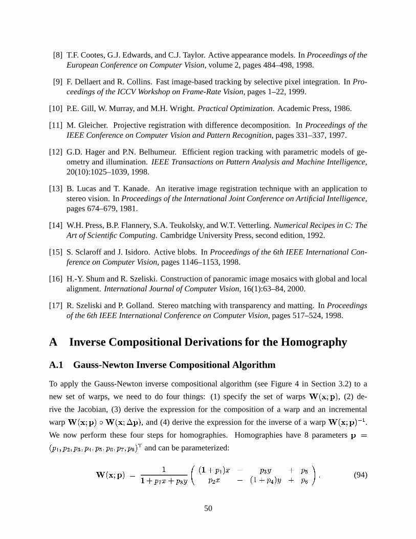
[8] T.F. Cootes, G.J. Edwards, and C.J. Taylor. Active appearance models. In Proceedings of theEuropean Conference on Computer Vision, volume 2, pages 484–498, 1998.

[9] F. Dellaert and R. Collins. Fast image-based tracking by selective pixel integration. In Pro-ceedings of the ICCV Workshop on Frame-Rate Vision, pages 1–22, 1999.

[10] P.E. Gill, W. Murray, and M.H. Wright. Practical Optimization. Academic Press, 1986.

[11] M. Gleicher. Projective registration with difference decomposition. In Proceedings of theIEEE Conference on Computer Vision and Pattern Recognition, pages 331–337, 1997.

[12] G.D. Hager and P.N. Belhumeur. Efficient region tracking with parametric models of ge-ometry and illumination. IEEE Transactions on Pattern Analysis and Machine Intelligence,20(10):1025–1039, 1998.

[13] B. Lucas and T. Kanade. An iterative image registration technique with an application tostereo vision. In Proceedings of the International Joint Conference on Artificial Intelligence,pages 674–679, 1981.

[14] W.H. Press, B.P. Flannery, S.A. Teukolsky, and W.T. Vetterling. Numerical Recipes in C: TheArt of Scientific Computing. Cambridge University Press, second edition, 1992.

[15] S. Sclaroff and J. Isidoro. Active blobs. In Proceedings of the 6th IEEE International Con-ference on Computer Vision, pages 1146–1153, 1998.

[16] H.-Y. Shum and R. Szeliski. Construction of panoramic image mosaics with global and localalignment. International Journal of Computer Vision, 16(1):63–84, 2000.

[17] R. Szeliski and P. Golland. Stereo matching with transparency and matting. In Proceedingsof the 6th IEEE International Conference on Computer Vision, pages 517–524, 1998.

A Inverse Compositional Derivations for the Homography

A.1 Gauss-Newton Inverse Compositional Algorithm

To apply the Gauss-Newton inverse compositional algorithm (see Figure 4 in Section 3.2) to a

new set of warps, we need to do four things: (1) specify the set of warps �!�#"%$&�, (2) de-

rive the Jacobian, (3) derive the expression for the composition of a warp and an incremental

warp ��#"G$4� � ��#" � $&� , and (4) derive the expression for the inverse of a warp �!�#"%$&� / *.

We now perform these four steps for homographies. Homographies have 8 parameters$ �B(:*,�E(�=.� (�LK�E(1OK� (�M.�E(�P/�E(��/�E(��,�F�

and can be parameterized:

��#"%$&�5 ��N7<(�� 7<(�� 6 �G�N7<(H* � � 7 (1L�� 7 (�M(�= � 7 �G�N7<(1O.� � 7 (�P > - (94)

50

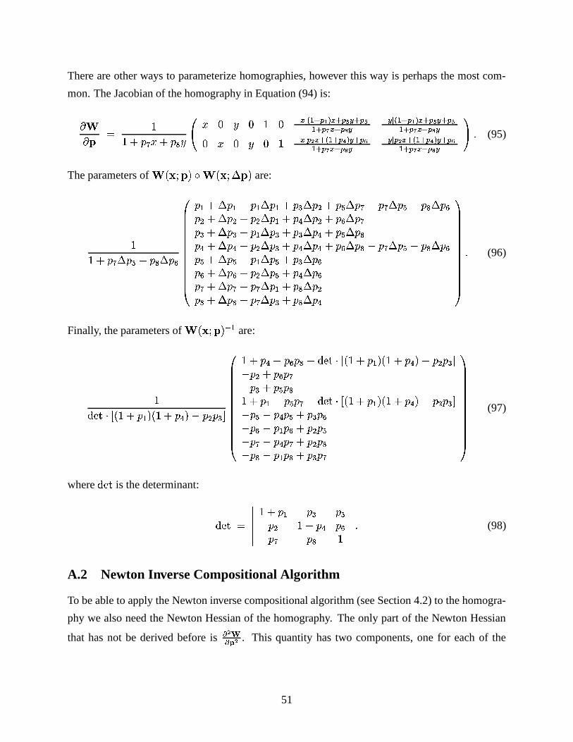
There are other ways to parameterize homographies, however this way is perhaps the most com-

mon. The Jacobian of the homography in Equation (94) is:

� � $ ��N7<(�� 7<(�� RT � ) � ) � ) / �� *�� ! � � �� *�� / �� *�� "! � � �� *�� ) � ) � ) � / �� $ � � � *�� *�� / �� $ � � � *�� *�� UY - (95)

The parameters of �!�#"%$&�� 3" � $4� are:

��N79(�� (�M37<(�� (�PRSSSSSSSSSSSSST

(H* 7 � (H*J79(:* � (:*J7<(�L � (�=�79(�M � (��&a5(�� (�M4a5(�� (�P(�=�7 � (�=�79(1= � (:*J7<(1O � (�=�79(�P � (��(�L�7 � (�L�79(:* � (1L�7<(�L � (1O379(�M � (��(1O�7 � (1O379(1= � (1L�7<(1O � (1O379(�P � (��4a5(�� (�M4a5(�� (�P(�M�7 � (�M�79(:* � (1M�7<(�L � (�P(�P�7 � (�P�79(1= � (1M�7<(1O � (�P(��J7 � (��79(�� (:*J7<(�� (�=(��7 � (��79(�� (1L�7<(�� (1OU WWWWWWWWWWWWWY-

(96)

Finally, the parameters of �!�#"%$&� / *are:

�� I _ ��Q7<(H* � �G�N79(1O,�Ja (�=E(�L�bRSSSSSSSSSSSSST

�N79(1ONa (�PE(��&a �� I _ ��479(H*D� �G�N79(1O,�Ja (�=E(�L�ba4(1=37<(�PF(��a4(1L37<(�MF(��N79(H*#a (�ME(��#a �� I _ ��479(H*D� �G�N79(1O,�Ja (�=E(�L�ba4(1MNa (1OE(�M37<(�LE(�Pa4(1PNa (H*!(�P37<(�=E(�Ma4(��4a (1OE(��7<(�=E(��a4(��Na (H*!(��37<(�LE(��UXWWWWWWWWWWWWWY

(97)

where��

is the determinant:

�� Q7<(H* (�L (1M(�= �Q7<(1O (1P(�� (�� - (98)

A.2 Newton Inverse Compositional Algorithm

To be able to apply the Newton inverse compositional algorithm (see Section 4.2) to the homogra-

phy we also need the Newton Hessian of the homography. The only part of the Newton Hessian

that has not be derived before is� $ �� $ . This quantity has two components, one for each of the

51

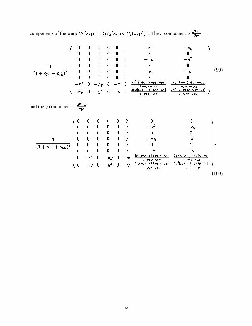
components of the warp ��3"%$4�� #"%$&� �� #"G$4�G�F� . The�

component is� $ �� $

��N79(��%� 79(��%�:� =RSSSSSSSSSSSSSST

) ) ) ) ) ) a�� = a ��) ) ) ) ) ) ) )) ) ) ) ) ) a�� a�� =) ) ) ) ) ) ) )) ) ) ) ) ) a�� a��) ) ) ) ) ) ) )a�� = ) a �� ) a � ) = � $ � � *�� "! � � �� *�� = �� *�� ! � � �� *�� a�� ) a � = ) a�� ) = �� *�� ! � � � � � � � � �*�� = � $ � � *�� ! � � � � � � � � �*��

U WWWWWWWWWWWWWWY(99)

and the�

component is� $ � (�� $

��Q7<(��%� 79(�� =RSSSSSSSSSSSSSST

) ) ) ) ) ) ) )) ) ) ) ) ) a � = a ��) ) ) ) ) ) ) )) ) ) ) ) ) a �� a�� =) ) ) ) ) ) ) )) ) ) ) ) ) a � a��) a � = ) a �� ) a�� = � $ � � $ � � � *�� *�� = �� %$ � � � *�� *�� ) a �� ) a�� = ) a � = �� $ � � � *�� *�� = � $ � � $ � � � *�� *��

U WWWWWWWWWWWWWWY-

(100)

52

Lucas-Kanade 20 Years On: A Unifying Framework Part 1: The ... · Lucas-Kanade 20 Years On: A...

Documents

Transcript of Lucas-Kanade 20 Years On: A Unifying Framework Part 1: The ... · Lucas-Kanade 20 Years On: A...