LTRC Project Number: 08-6GT State Project Number: 739 … · Performance of Buried Pipe...
123
1. Report No. FHWA/LA.10/467 2. Government Accession No. 3. Recipient's Catalog No. 4. Title and Subtitle Performance of Buried Pipe Installation 5. Report Date May 2010 6. Performing Organization Code LTRC Project Number: 08-6GT State Project Number: 739-99-1520 7. Author(s) Michele Barbato, Ph.D. Assistant Professor email: [email protected] 8. Performing Organization Report No. 9. Performing Organization Name and Address Department of Civil and Environmental Engineering Louisiana State University Baton Rouge, LA 70803 10. Work Unit No. 11. Contract or Grant No. 12. Sponsoring Agency Name and Address Louisiana Department of Transportation and Development P.O. Box 94245 Baton Rouge, LA 70804-9245 13. Type of Report and Period Covered Final Report Period Covered 01-2008 – 12-2009 14. Sponsoring Agency Code 15. Supplementary Notes Conducted in Cooperation with the U.S. Department of Transportation, Federal Highway Administration 16. Abstract The purpose of this study is to determine the effects of geometric and mechanical parameters characterizing the soil structure interaction developed in a buried pipe installation located under roads/highways. The drainage pipes or culverts installed as part of a roadway project are considered as holistic systems which include not only the pipes and their mechanical properties as determined by materials, geometry and manufacturing procedures, but also the natural soil and the trench into which the pipe is placed, constructed and expected to perform. The research results confirm that the performance of the soil-structure interaction system constituted by the pipe, the trench backfill and the natural soil surrounding the trench depends significantly not only on the pipe material and stiffness but also on geometric parameters defining the trench in which the pipe is installed, such as cover height, bedding thickness and trench width. Minimum requirements for these geometric parameters can be established to obtain equivalent performances of different pipe systems as function of (1) the pipe stiffness and diameter, (2) the local natural soil properties, and (3) the type of road pavement. The results of this research can be used as guidance in establishing guidelines for the alternate selection and application of typical highway drainage products, such as pipes and culverts. This report provides initial data that can be used for a proper comparison of performance, in terms of deformations of the road surface under typical loads, of pipes characterized by different materials and different installation geometry and methodologies. This project suggests also future research directions to delineate a rigorous comparison of different soil-pipe systems under a more general definition of performance, rigorously accounting for economical factors (e.g., initial cost, life-cycle cost) and societal risk. 17. Key Words Buried pipes; culverts; soil-structure interaction; finite element method 18. Distribution Statement Unrestricted. This document is available through the National Technical Information Service, Springfield, VA 21161. 19. Security Classif. (of this report) 20. Security Classif. (of this page) 21. No. of Pages 123 22. Price TECHNICAL REPORT STANDARD PAGE
Transcript of LTRC Project Number: 08-6GT State Project Number: 739 … · Performance of Buried Pipe...

1. Report No. FHWA/LA.10/467
2. Government Accession No. 3. Recipient's Catalog No.
4. Title and Subtitle Performance of Buried Pipe Installation
5. Report Date
May 2010 6. Performing Organization Code LTRC Project Number: 08-6GT State Project Number: 739-99-1520
7. Author(s)
Michele Barbato, Ph.D. Assistant Professor email: [email protected]
8. Performing Organization Report No.
9. Performing Organization Name and Address Department of Civil and Environmental Engineering Louisiana State University Baton Rouge, LA 70803
10. Work Unit No.
11. Contract or Grant No.
12. Sponsoring Agency Name and Address
Louisiana Department of Transportation and Development P.O. Box 94245 Baton Rouge, LA 70804-9245
13. Type of Report and Period Covered
Final Report Period Covered 01-2008 – 12-2009 14. Sponsoring Agency Code
15. Supplementary Notes
Conducted in Cooperation with the U.S. Department of Transportation, Federal Highway Administration
16. Abstract
The purpose of this study is to determine the effects of geometric and mechanical parameters characterizing the soil structure interaction developed in a buried pipe installation located under roads/highways. The drainage pipes or culverts installed as part of a roadway project are considered as holistic systems which include not only the pipes and their mechanical properties as determined by materials, geometry and manufacturing procedures, but also the natural soil and the trench into which the pipe is placed, constructed and expected to perform. The research results confirm that the performance of the soil-structure interaction system constituted by the pipe, the trench backfill and the natural soil surrounding the trench depends significantly not only on the pipe material and stiffness but also on geometric parameters defining the trench in which the pipe is installed, such as cover height, bedding thickness and trench width. Minimum requirements for these geometric parameters can be established to obtain equivalent performances of different pipe systems as function of (1) the pipe stiffness and diameter, (2) the local natural soil properties, and (3) the type of road pavement. The results of this research can be used as guidance in establishing guidelines for the alternate selection and application of typical highway drainage products, such as pipes and culverts. This report provides initial data that can be used for a proper comparison of performance, in terms of deformations of the road surface under typical loads, of pipes characterized by different materials and different installation geometry and methodologies. This project suggests also future research directions to delineate a rigorous comparison of different soil-pipe systems under a more general definition of performance, rigorously accounting for economical factors (e.g., initial cost, life-cycle cost) and societal risk. 17. Key Words
Buried pipes; culverts; soil-structure interaction; finite element method
18. Distribution Statement Unrestricted. This document is available through the National Technical Information Service, Springfield, VA 21161.
19. Security Classif. (of this report)
20. Security Classif. (of this page)
21. No. of Pages
123 22. Price
TECHNICAL REPORT STANDARD PAGE


2
Project Review Committee
Each research project will have an advisory committee appointed by the LTRC Director. The
Project Review Committee is responsible for assisting the LTRC Administrator or Manager
in the development of acceptable research problem statements, requests for proposals, review
of research proposals, oversight of approved research projects, and implementation of
findings.
LTRC appreciates the dedication of the following Project Review Committee Members in
guiding this research study to fruition.
LTRC Administrator
Zhongjie “Doc” Zhang, Ph.D., P.E.
Pavement & Geotech Research Administrator
Members
Luanna Cambas
Brian Buckel
JoAnn Kurts
Steven Cumbaa
Arturo Aguirre
Khalid Farrag
Directorate Implementation Sponsor
Richard Savoie


Performance Evaluation of Buried Pipe Installation
by
Michele Barbato, Ph.D.
Marvin Bowman Alexander Herbin
Civil and Environmental Engineering
3531 Patrick F. Taylor Hall
Louisiana State University
Baton Rouge, Louisiana 70803
LTRC Project No. 08-6GT
State Project No. 739-99-1520
conducted for
Louisiana Department of Transportation and Development
Louisiana Transportation Research Center
The contents of this report reflect the views of the author/principal investigator who is
responsible for the facts and the accuracy of the data presented herein. The contents of this
report do not necessarily reflect the views or policies of the Louisiana Department of
Transportation and Development or the Louisiana Transportation Research Center. This
report does not constitute a standard, specification, or regulation.
May 2010


iii
ABSTRACT
The purpose of this study was to determine the effects of geometric and mechanical
parameters characterizing the soil structure interaction developed in a buried pipe installation
located under roads/highways. The drainage pipes or culverts installed as part of a roadway
project are considered as holistic systems that include not only the pipes and their mechanical
properties as determined by materials, geometry, and manufacturing procedures, but also the
natural soil and the trench into which the pipe is placed, constructed, and expected to
perform. The research results confirmed that the performance of the soil-structure interaction
system constituted by the pipe, the trench backfill, and the natural soil surrounding the trench
depends significantly not only on the pipe material and stiffness but also on geometric
parameters defining the trench in which the pipe is installed, such as cover height, bedding
thickness, and trench width. Minimum requirements for these geometric parameters can be
established to obtain equivalent performances of different pipe systems as function of (1) the
pipe stiffness and diameter, (2) the local natural soil properties, and (3) the type of road
pavement.
The results of this research can be used as guidance in establishing guidelines for the
alternate selection and application of typical highway drainage products, such as pipes and
culverts. This report provides initial data that can be used for a proper comparison of
performance, in terms of deformations of the road surface under typical loads, of pipes
characterized by different materials and different installation geometry and methodologies.
This project also suggests future research directions to delineate a rigorous comparison of
different soil-pipe systems under a more general definition of performance, rigorously
accounting for economical factors (e.g., initial cost, life-cycle cost) and societal risk.


v
ACKNOWLEDGMENTS
Financial support of this research project by the Louisiana Department of Transportation and
Development (LADOTD) through the Louisiana Transportation Research Center (LTRC) is
gratefully acknowledged.
The authors would also like to thank Zhongjie Zhang, Ph.D., P.E., LTRC project manager,
who provided guidance for all phases of the research project; the project review committee
members, who provided comments and feedback for the research; and Brian Felder, Joe
Babcanec, and Mark Joersz from ADS/Hancor, Inc., who provided the geometrical
information needed to accurately model high-density polyethylene (HDPE) pipes.


vii
IMPLEMENTATION STATEMENT
The results of this research can be used as guidance in establishing guidelines for the
alternate selection and application of typical highway drainage products, such as pipes and
culverts. This report provides initial data that can be used for a rigorous comparison, in terms
of deformations of the road surface and pipe ring deformation under typical loads, of the
performance of pipes characterized by different materials and different installation geometry
and methodologies. This project also suggests future research directions to delineate a
rigorous comparison of different soil-pipe systems under a more general definition of
performance, rigorously accounting for economical factors (e.g., initial cost, life-cycle cost)
and societal risk.
The following specific recommendations are made for implementation:
1) The minimum cover height should be expressed as a function of the pipe diameter.
2) For flexible and semi-flexible pipes, the minimum trench width should be equal to twice
the pipe diameter, while for rigid pipes a minimum trench width equal to the pipe
diameter + 3 ft. is sufficient.
3) Different minimum requirements can be made for yielding and stiff soils. In the absence
of specific data from in-situ tests, the more demanding requirements for yielding soil
should be followed in favor of safety.
4) Different minimum requirements can be made for different road pavements with more
demanding requirements for more flexible road pavements.

ix
TABLE OF CONTENTS
ABSTRACT ............................................................................................................................. iii
ACKNOWLEDGMENTS .........................................................................................................v
IMPLEMENTATION STATEMENT .................................................................................... vii
TABLE OF CONTENTS ......................................................................................................... ix
LIST OF TABLES ................................................................................................................... xi
LIST OF FIGURES ............................................................................................................... xiii
INTRODUCTION .....................................................................................................................1
OBJECTIVE ..............................................................................................................................5
SCOPE .......................................................................................................................................7
METHODOLOGY ....................................................................................................................9
Linear FE Modeling of Buried Pipe Installations ....................................................... 10 Description of the FE models Employed ........................................................ 10 Simplifying Assumptions and Limitations of the Performed Linear Elastic FE Analyses ........................................................................................ 12
Model Dimension Sensitivity Study ........................................................................... 13 Nonlinear FE Modeling of Buried Pipe Installations ................................................. 14
Nonlinear FE Model Description .................................................................... 16 Nonlinear Hysteretic Material Constitutive Models ....................................... 20 Loading Conditions and Nonlinear FE Staged Analysis ................................ 21
DISCUSSION OF RESULTS..................................................................................................23
Sensitivity Analysis of Buried Pipe Installation Performance Based on Linear Elastic FE Analysis ..................................................................................................... 23
Sensitivity to Trench Excavation Width: W ................................................... 25 Sensitivity to Soil Cover Height: Hc ............................................................... 28 Sensitivity to Bedding Thickness: Hb ............................................................. 29 Sensitivity to Initial Stiffness of Natural Soil Surrounding the Trench: Es .... 30 Sensitivity to Backfill Material Stiffness: Ef .................................................. 31 Sensitivity to Pipe Geometry: Pipe Diameter, D, and Pipe Thickness, t ........ 32 Sensitivity to Road Pavement Type ................................................................ 33
Identification of Cases of Possible Insufficient Performance via Linear Elastic FE Analysis ................................................................................................................. 34 Model Dimension Sensitivity Analysis Results .......................................................... 35 Validation and Verification of Results via Nonlinear Hysteretic FE Analysis .......... 37
Nonlinear FE Analysis Results for RC Pipes ................................................. 39 Nonlinear FE Analysis Results for Steel Pipes ............................................... 43 Nonlinear FE Analysis Results for PVC Pipes ............................................... 44 Nonlinear FE Analysis Results for HDPE Pipes ............................................ 46 Comparison of Deflections for FE Models with Optimal Hc vs. Minimum Hc ................................................................................................... 47
CONCLUSIONS......................................................................................................................53
RECOMMENDATIONS .........................................................................................................57

x
ACRONYMS, ABBREVIATIONS, & SYMBOLS ................................................................59
REFERENCES ........................................................................................................................61
APPENDIX A ..........................................................................................................................63
Nonlinear FE Results for Overall Comparisons ......................................................... 63 APPENDIX B ..........................................................................................................................95
Comparison of Results from Optimal Cover vs. Minimal Cover ............................... 95

xi
LIST OF TABLES
Table 1 Total number of models……………………………………………………..…….15
Table 2 Total number of elements, nodes, and degrees-of-freedom (DOFs) with running
with running time for each nonlinear hysteretic FE model……..…………….….15
Table 3 Linear elastic FE analyses parameters………………………………………..…...24
Table 4 Summary of optimal Hc vs. LADOTD minimum Hc………………………….......48
Table 5 Comparison of variation in Δlive and ΔR,live when using optimal Hc vs. LADOTD
Hc vs. LADOTD minimum Hc………………...……………………………..…..49
Table 6 Comparison of variation of Δ and ΔR when using optimal
Hc vs. LADOTD minimum Hc………………………………………………..…..50
Table 7 Displacements at the pipe’s crest and bottom, top and bottom, due to both gravity
due to both gravity and live loads………………………………………………...51
Table 8 Comparison of diameter changes due to both gravity and live loads……………52


xiii
LIST OF FIGURES
Figure 1 Buried pipe installation: (a) transversal view (cross-section) and
(b) longitudinal view. .............................................................................................. 2
Figure 2 Description of a typical linear elastic FE model: (a) schematic representation of
the regions and boundary conditions, and (b) regions modeled through
isoparametric triangular elements. ........................................................................ 11
Figure 3 Subdivision into different zones (“parts” and “regions”) of the nonlinear FE
model in ABAQUS: (a) part modeling the pipe, and (b) part modeling the
remaining components of the system. ................................................................... 17
Figure 4 Pipe profiles: (a) RC pipe, (b) steel pipe, (c) PVC pipe, and (d) HDPE pipe. ...... 18
Figure 5 Different sub-regions in the nonlinear FE models. ............................................... 18
Figure 6 Nonlinear FE model mesh: (a) complete model, and (b) zoom view of the pipe,
haunch, and crown regions. .................................................................................. 19
Figure 7 Boundary conditions: (a) bottom surface, (b) front and back surfaces, and
(c) side surfaces. .................................................................................................... 20
Figure 8 Sensitivity study: effects of trench excavation width (moderately stiff natural
soil). ...................................................................................................................... 26
Figure 9 Sensitivity study: effects of trench excavation width (moderately stiff
natural soil and very stiff backfill material). ......................................................... 26
Figure 10 Sensitivity study: effects of trench excavation width (yielding natural soil). ....... 27
Figure 11 Sensitivity study: effects of soil cover height. ....................................................... 28
Figure 12 Sensitivity study: effects of bedding thickness with soft bedding material. ......... 29
Figure 13 Sensitivity study: effects of bedding thickness with stiff bedding material. ......... 30
Figure 14 Sensitivity study: effects of initial stiffness of natural soil surrounding the
trench..................................................................................................................... 31
Figure 15 Sensitivity study: effects of initial stiffness of backfill material (i.e., grade of
compaction)........................................................................................................... 32
Figure 16 Sensitivity study: effects of pipe diameter. ........................................................... 32
Figure 17 Sensitivity study: effects of pipe ring stiffness (i.e., pipe thickness). ................... 33
Figure 18 Sensitivity study: effects of different pavement type. ........................................... 34
Figure 19 Model dimension sensitivity study: variation of deflection response at the road
surface for the 3-D FE of a soil-pipe system with a HDPE pipe of
diameter D = 60 in. ............................................................................................... 36
Figure 20 Model dimension sensitivity study: variation of maximum stress in the
pipe for the 3-D FE of a soil-pipe system with a HDPE pipe of diameter
D = 60 in. .............................................................................................................. 37

xiv
Figure 21 Locations at which the FE response is monitored for computing the performance
measures: (a) monitored deflection at the road surface (profile of ∆) and (b)
reference system for ∆R measurement .................................................................. 38
Figure 22 Profile of due to live loads only (live) for RC pipe with D = 42 in ................... 39
Figure 23 Profile of due to live loads only (live) for RC pipe with D = 42 in:
zoom view ............................................................................................................. 39
Figure 24 Profile of due to plastic deformation (inelastic) for RC pipe with D = 42 in ...... 40
Figure 25 Comparison of R due to live loads only (R,live) for RC pipe with D = 42 in ...... 41
Figure 26 Profile of due to live loads only (live) for RC pipe with D = 60 in ................... 41
Figure 27 Profile of due to live loads only (live) for RC pipe with D = 60 in: zoom
view ....................................................................................................................... 42
Figure 28 Profile of due to plastic deformation (inelastic) for RC pipe with D = 60 in ...... 42
Figure 29 Comparison of R due to live loads only (R,live) for RC pipe with D = 60 in ...... 43
Figure 30 Profile of due to live loads only (live) for steel pipe with D = 42 in: zoom
view ....................................................................................................................... 44
Figure 31 Profile of due to live loads only (live) for steel pipe with D = 60 in: zoom
view ....................................................................................................................... 44
Figure 32 Profile of due to live loads only (live) for PVC pipe with D = 42 in: zoom
view ....................................................................................................................... 45
Figure 33 Profile of due to live loads only (live) for PVC pipe with D = 60 in: zoom
view ....................................................................................................................... 45
Figure 34 Profile of due to live loads only (live) for HDPE pipe with D = 42 in: zoom
view ....................................................................................................................... 46
Figure 35 Profile of due to live loads only (live) for HDPE pipe with D = 60 in: zoom
view ....................................................................................................................... 47
Figure 36 Comparison of profile of due to live loads only (live) for all pipes with
D = 42 in: zoom view .......................................................................................... 47
Figure 37 Comparison of profile of due to live loads only (live) for all pipes with
D = 60 in: zoom view ........................................................................................... 48
Figure 38 Comparison of undeformed and deformed pipe shape: (a) total deflections of the
FE model, and (b) relative deflection of the pipe ring with respect to the
undeformed pipe ................................................................................................... 51
Figure 39- Figure 124………………………….……………...……...Appendixes (p. 63-105)

INTRODUCTION
Existing codes and recommendations often require standard/minimum values for the
bedding, backfill, and fill cover geometric and mechanical properties in the installation of
buried pipes under transportation facilities. These recommended values are often obtained by
considering the worst-case scenario for each of the components and account only in an
approximate way for the soil-structure interaction (SSI) between bedding, backfill, fill cover,
and pipes of different materials and mechanical properties. Performance in terms of
reliability and cost-effectiveness of the design is not fully addressed by the current
specifications. The need arises for revising the current specifications to obtain a more
efficient design of the installation of buried pipes.
Current design methodologies for buried pipes are still based on the Marston theory,
developed between 1930 and 1960, for estimating vertical loads [1]. This design method is
based on the assumption of an elastic, isotropic soil above and around the pipe. Such an
approach has been deemed as over-conservative, given the simplifications associated with
these inherent assumptions. In addition, the method does not consider the effects of different
bedding material and thickness.
Some preliminary research has been performed on concrete box culverts at the University of
Texas at Arlington. This research involves the experimental investigation of the shear
capacity of precast reinforced concrete box culverts [2]. The Pennsylvania Department of
Transportation has conducted a study on the effect of bedding thickness to investigate
problems they experienced. This study was not published. The Federal Highway
Administration (FHWA) sponsored research at UMass that investigated the use of soft
bedding to reduce soil pressure at the invert, but this study did not investigate the depth of
bedding as a variable. Among other results, this research led to the development of Culvert
Analysis and Design (CANDE). CANDE is a two-dimensional nonlinear finite element (FE)
buried pipe and culvert software application used for the structural design, analysis, and
evaluation of buried pipes, culverts, and other soil-structure interaction systems [3, 4]. The
FE program has been continuously extended (e.g., by including AutoCAD interfaces in
CandeCAD Pro) and incorporates built-in linear and nonlinear soil and pipe material models
to analyze almost any type of installation. FE analysis studies using the SSI program Soil-
Pipe Interaction and Design Analysis (SPIDA) have been conducted for and implemented
into AASHTO LRFD Bridge Design Specifications, Section 12 [5]. Results are used for
defining standard installations, bedding thickness, and minimum compaction requirements

2
but are mostly obtained from conservative assumptions and referred to as deep cover
situations.
The buried pipe installation considered in this project is a trench type with vertical walls and
a single pipe (Figure 1). This type of installation involves the removal of a trench of natural
soil in which a bedding layer, the pipe, and different layers of backfill materials are
positioned. After the trench is filled and the backfill material is compacted, the sub-pavement
and the road pavement (asphalt or concrete) are laid over the trench and the surrounding
natural soil. The installation is characterized by shallow cover. Therefore, the live loads due
to the vehicular traffic produce significant stresses on the pipe and the soil in the trench, with
a stress distribution strongly dependent on the specific geometric and mechanical properties
of the entire soil-pipe system.
Figure 1
Buried pipe installation: (a) transversal view (cross-section) and (b) longitudinal view
This project proposes the use of a linear and nonlinear FE analysis to investigate the effects
of the geometric and mechanical parameters characterizing the soil-structure interaction
developed in a buried pipe installation. Adoption of FE modeling to analyze such problems
in geomechanics is not new and has increased in reliability and practicality as the analysis
tools and computational power have evolved. The adoption of a numerical approach is a
P
W
Bedding
Pavement
Cover
Backfill
D
Hb
Hc
Hp
t
Pavement Base (Sub-pavement)Hs
Natural soil
Traffic load Traffic direction
P
Bedding
Pavement
Cover
Pipe
D
Hb
Hc
Hp
Pavement Base (Sub-pavement)Hs
Natural soil
Traffic load
P
Pipe axis
(a) (b)

3
justifiable choice, considering the number of parameters involved and the complex
interaction between the response of the soil and pipe.
This research presents several innovative aspects compared to previous similar studies. In
particular, this study (a) focuses on pipes and culverts buried in shallow cover conditions; (b)
considers soil conditions (i.e., soft cohesive soils) typical of Southern Louisiana; (c) models
explicitly the effects of different road pavements and sub-pavements; (d) introduces a new
performance parameter corresponding to the dip depth at the road surface produced by the
live loads due to traffic; and (e) provides an extensive parametric study to evaluate the
performance sensitivity of the soil-pipe system to material, mechanical, and geometric
parameters defining pipes, trench backfills, natural soils, and road pavement types.


5
OBJECTIVE
The goal of this research project was to determine the effects of geometric and mechanical
parameters characterizing the soil-structure interaction developed in buried pipe installations.
Parameters such as pipe ring stiffness, bedding thickness, trench width, and fill cover height
were considered.
The specific objectives of this study were: (1) to provide a rigorous sensitivity analysis to
various geometric and mechanical parameters of the performance of buried pipe installations
in terms of deformation and stresses in the pipe and deformation (dip depth) at the surface of
transportation facility pavement; (2) to derive preliminary results that can be used as an
initial justification for accepting/revising the current provisions for minimum bedding
thickness, fill cover height, and installation quality for pipes buried under transportation
facilities; and (3) to provide guidelines for developing a set of recommendations for
minimum/optimal requirements on cover height, bedding thickness, and trench width that
ensure similar performance for pipes of different materials, i.e., reinforced concrete (RC),
steel, polyvinyl chloride (PVC), and high density polyethylene (HDPE).


7
SCOPE
The scope of this research included the study of the mechanical behavior of buried culvert
and pipes. The considered pipes are buried in trenches excavated below roads with different
levels of transit. The local soil conditions in which the pipes are installed are representative
of typical locations in Southern Louisiana, i.e., with soft clay. Only single pipe installations
were considered. The pipe dimensions studied cover the range between 18 in. and 60 in. of
pipe internal diameters. Different materials were considered for the pipes, i.e., reinforced
concrete, steel, PVC, and HDPE. This research focused on culvert pipes buried in shallow
cover situations where traffic creates a high live load influence on the pipe. The geometrical
properties (circular shape, thickness, and diameter ranges) considered in this investigation are
representative of typical drainage pipes and culverts constructed on LADOTD projects and
do not include box culvert or three sided structures.
Only loadings from traffic were considered and modeled as static equivalent loads applied on
the surface of the road. These loads were amplified by using an appropriate dynamic impact
factor to approximately account for dynamic effect. The soil-structure interaction behavior
between the pipe, the backfill material, and the natural soil surrounding the trench was
explicitly modeled and included in the study. Only short-term loading effects were
considered. Effects of repeated loading cycles (i.e., fatigue) were not analyzed in this
research.
The results of this research are intended to be used as input for cost-benefit analyses for
alternate bidding of buried pipes of different materials. However, a complete cost-benefit
analysis is outside the scope of this research. It should be noted that a complete cost-benefit
analysis must consider (in addition to the direct costs of pipes and backfill material,
excavation, installation of the pipe, filling of the trench, and compaction of the backfill
material) costs associated with: (1) different hydraulic capacity of same-size different-
material pipes (i.e., for the same transportation facility, pipes of different materials could also
be a different size in order to satisfy the hydraulic requirements of the design); (2) protection
from corrosion (e.g., cathodic protection and grouting) of metallic parts; and (3) other labor
associated with ensuring the long-term performance of the buried pipe installations. These
are not directly related to the short-term mechanical performance of buried pipe installations
and were not considered in this study. However, these costs must be included in the cost-
benefit analysis of a specific installation.

9
METHODOLOGY
A study of the SSI between pipes, trench backfill, and natural soil based on the FE method
was completed during this research. The FE method allows for an accurate analysis of the
complex interaction between the pipe, the trench backfill material, and the surrounding
natural soil under different conditions, characterized by a wide range of geometric and
mechanical parameters.
Appropriate FE models of pipes buried in shallow trenches and positioned below roadways
were built using different commercial FE codes to study the sensitivity of the mechanical
behavior of the soil-pipe system for a wide range of conditions typically encountered in
highway projects in Southern Louisiana. A simplified linear elastic FE analysis was
employed to perform an extensive parametric study and sensitivity analysis of soil-pipe
installation systems. An advanced nonlinear hysteretic FE analysis was used (a) to validate
the linear elastic FE analysis results under the specific conditions representing a proposed
modification to the current LADOTD requirements for LADOTD highway projects, (b) to
accurately evaluate the sensitivity of a buried pipe system performance to modeling
parameters and SSI effects, and (c) to investigate in detail the combinations of parameter
values for which the performance of the soil-pipe installation system may be unsatisfactory.
This research project studied the effects on buried pipe performance due to: 1) Excavation width (W);
2) Fill cover height (Hc);
3) Bedding height (Hb);
4) Mechanical properties (e.g., stiffness: Es, cohesion: cs, friction angle: s) of the natural soil surrounding the trench;
5) Mechanical properties and grade of compaction (e.g., stiffness: Ef, cohesion: cf, friction angle: f) of the fill material;
6) Mechanical properties and grade of compaction (e.g., stiffness: Eb, cohesion: cb, friction angle: b) of the bedding material;
7) Pipe material (RC, steel, PVC, and HDPE), mechanical properties (e.g., stiffness: E, and yield strength: y), and geometric properties (diameter: D and thickness: t) of the pipe;
8) Material (concrete or asphalt) and geometry of the roadway pavement (road pavement thickness: Hp) and its sub-pavement (sub-pavement thickness: Hsp, and sub-pavement stiffness: Esp); and
9) Importance of facility (different loadings and different requirements on deformation performance).

10
The pipe performance has been defined in terms of relevant quantities characterizing the FE
response of the soil-pipe system such as:
1) Maximum radial deformation (R) of the pipe (deformation performance); and
2) Maximum dip depth (live) at the surface (driver comfort and safety performance) under maximum design load.
Linear FE Modeling of Buried Pipe Installations
Linear elastic FE analyses were performed by using the commercial FE program SAP2000,
typically employed in the civil engineering and structural engineering communities for FE
analysis of structural and soil-structure interaction systems subjected to static and dynamic
loadings [6]. This program was chosen for this part of the project due to its advanced and
user-friendly graphical user interface, its simplicity of use, and its high computational speed,
particularly for problems characterized by linear elastic behavior and large meshes (i.e.,
linear elastic FE models with a large number of finite elements and degrees of freedom). The
next sections of this report describe the linear elastic FE models built in SAP2000, the
analyses performed, the simplifying modeling assumptions adopted, and the corresponding
limitations in the obtained results.
Description of the FE models Employed
Two-dimensional (2-D) models of typical cross-sections (Figure 2a) were built to study the
performance of the soil-pipe installation under a wide range of different conditions and
geometries. Making use of the symmetry of the cross-section model, the 2-D models
included explicitly only one half of the trench. The soil-pipe system was modeled under plain
strain conditions and the thickness of the model was assumed equal to one foot. The soil in
the trench, the sub-pavement layer, and the road pavement were modeled using isoparametric
quadrilateral elements with bilinear interpolation of the displacement fields, with the
exception of the parts of the model immediately surrounding the pipe, where isoparametric
triangular elements were employed (Figure 2b). The material used to fill the trench was
subdivided into different layers, i.e., bedding, backfill, and cover. Different Young’s moduli
were employed to model the different mechanical behavior of each layer.
The pipe was modeled by using ordinary displacement-based Euler-Bernoulli frame
elements. The frame element cross-sectional properties were obtained from the cross-
sectional area and second moment of inertia of the pipe ring corresponding to one linear foot
of pipe and computed about its centerline. The Young’s modulus of the pipe was obtained

11
from the pipe material properties provided by American Association of State Highway and
Transportation Officials (AASHTO) standards.
Figure 2
Description of a typical linear elastic FE model: (a) schematic representation of the
regions and boundary conditions and (b) regions modeled through isoparametric
triangular elements
The natural soil surrounding the trench was modeled indirectly through appropriate boundary
conditions applied along the borders of the FE model of the pipe-trench system. The
boundary conditions at the bottom and at the side of the trench in contact with the natural soil
were imposed through linear elastic vertical and horizontal springs with stiffness defined as a
function of the natural soil mechanical properties (Young’s modulus). The boundary
conditions along the plane of symmetry of the pipe installation were imposed in order to
consistently represent the symmetry conditions, i.e., the horizontal displacements through the
plane of symmetry were imposed equal to zero.
Both the self-weight of the different soil layers, pipe materials, and road surface, referred to
as “gravity loads” hereinafter, and traffic live loads were considered. The gravity loads were
obtained assuming a weight per unit volume equal to 124.8 lb/ft3 for the soil materials and
the weight per unit length of the pipe corresponding to the different pipe materials. The live
loads were obtained considering the axle load corresponding to a standard H20 truck load as
P
W
Bedding
Pavement
Cover
BackfillD
Hb
Hc
Hp
t
Pavement BaseHs
Bedding
Backfill
Cover
Pipe
Triangular FEs
(a)
(b)

12
defined in the AASHTO Standard Specifications for Highway Bridges [7]. The live loads
were applied statically to the FE model in correspondence of the plane of symmetry as a
concentrated load with intensity equal to one quarter of the AASHTO standard H20 truck
axle load (i.e., 16 kips / 4 = 4 kips). A dynamic impact factor equal to 1.50 was used to
approximately account for dynamic effects. It is noteworthy that the dynamic impact factor
value recommended by the AASHTO code is equal to 1.33. However, this study used a value
of 1.50 in order to account for below average road conditions (i.e., rough road surfaces) that
may be encountered in older road facilities. Thus, the load used in the FE model is equal to 6
kips. The discretization of the considered FE model was determined so to ensure mesh
independence of the response results.
Simplifying Assumptions and Limitations of the Performed Linear Elastic FE Analyses
Linear elastic FE analysis is computationally inexpensive when compared to more accurate
and realistic nonlinear hysteretic FE analysis. Indeed, each linear elastic FE analysis
performed in this study required less than one minute of computational time using an
ordinary personal computer. The reduced computational cost of a linear elastic analysis
allowed exploring a wide range of values of numerous geometric and mechanical parameters.
This extensive parametric study required about 25,000 FE analyses and provided important
information about the sensitivity of the performance of buried pipe installations. This
information is sufficiently accurate to qualitatively assess the conditions under which pipes
made of different materials can perform similarly, and thus can be used as alternative design
solutions.
Nevertheless, several simplifying assumptions were employed in the linear elastic FE
modeling of soil-pipe systems. Therefore, the analysis results are affected by some
limitations, which are briefly described below.
1) The soil and pipe materials were modeled as linear elastic. In general, this simplification
can lead to overestimating stresses and underestimating deformations. Also, long term
effects, nonlinear geometry, and local buckling were not modeled.
2) The effects of imperfect interface contact between the pipe and soil were neglected. This
assumption could overestimate the beneficial contribution of soil-structure interaction to
the performance of buried pipe installations.
3) The live loads due to vehicular traffic were modeled as a static concentrated load
magnified by a dynamic amplification factor. This approximation can lead to
conservative estimates of the stresses applied on the pipe, particularly for very shallow
trenches.

13
4) The effects of installation procedures and construction phases were neglected by simply
superposing the loads due to gravity and live loads. Accurate modeling of these effects
requires a staged nonlinear FE analysis faithfully reproducing the specific installation
procedure.
5) The soil surrounding the trench was indirectly modeled through elastic springs applied at
the boundaries of the trench model. This crude simplification can provide only a
qualitative estimate of the effects of different local soil conditions on the performance of
buried pipe installations.
6) Three-dimensional effects were neglected.
7) The effects of variable water elevation were not modeled explicitly. However, the range
of values for the initial stiffness of the backfill material was chosen in order to include
values representative of the two extreme cases of water level (below the bottom of the
trench and at the road surface level).
In order to overcome the above limitations and to validate the results obtained by using linear
elastic FE analysis, more advanced, accurate, and realistic nonlinear hysteretic FE models
were built and analyzed. The model size for the nonlinear hysteretic models was determined
based on a parametric study with respect to the dimensions of the model, referred to as the
model dimension sensitivity study hereafter.
Model Dimension Sensitivity Study
A model dimension sensitivity study was performed on the linear elastic FE models of buried
pipe installation systems. The objective of this sensitivity study was to determine the
appropriate dimensions for a three-dimensional (3-D) nonlinear hysteretic FE model in order
to obtain FE response results (e.g., pipe stresses/deformations and dip depth at the road
surface) insensitive to model dimensions. This study focused on determining (a) the size of
the appropriate expansion size of native soil to be included in the model in both horizontal
and vertical directions and (b) the thickness of the FE model.
The first part of the model dimension sensitivity study was performed based on the original
2-D models by removing the elastic springs used as boundary conditions to model the natural
soil surrounding the trench and replacing them with a FE model based on the mechanical
properties of the actual native soil. The effects of both horizontal (i.e., soil region on the side
of the trench) and vertical (i.e., soil region below the trench) native soil expansion were
considered. The FE model was increased in both directions, both independently and
simultaneously, with discrete increments equal to one quarter of the trench width in the

14
horizontal direction and 2 ft. in the vertical direction, until the changes in the FE results were
negligible.
A second step of the model dimension sensitivity study focused on the effects due to the
thickness of the FE model. The thickness of the 2-D elements was modified with discrete
increments equal to 6 in. until model dimension independence of the response results was
observed. The dimensions of the 2-D FE models obtained from this second sensitivity
analysis step were used as the starting point for the 3-D models.
The 3-D FE models were built using solid elements for both soil and pipe components. The
new FE models were obtained by extruding, in the direction parallel to the pipe axis, the
elements of the 2-D models. In this case, due to symmetry, only one quarter of the physical
soil-pipe system was modeled. Model dimension independence of the response results was
verified under appropriate boundary conditions.
In the 3-D FE models, the intensity of the live loads was kept equal to the intensity
considered in the 2-D model, while the point load was substituted by an equivalent uniformly
distributed load based on the AASHTO tire-road contact dimensions for an 18 wheel truck.
This contact surface is defined as a rectangular shape with sides equal to 12 in. and 7 in. [7].
The live loads in the 3-D model are transmitted to the road by a quarter of a tire, and the
uniform pressure is obtained by distributing the corresponding 6 kips load over a rectangular
area with sides equal to 6 in. and 3.5 in., respectively.
Nonlinear FE Modeling of Buried Pipe Installations
Nonlinear hysteretic FE models were built using the general purpose FE program ABAQUS.
ABAQUS is a widely used FE program suitable for linear and nonlinear FE analysis of
structural and mechanical systems subjected to static and/or dynamic loading conditions [8].
The program was chosen for the high reliability of its results, its versatility, and rich library
of FEs, material constitutive models, and solution strategies.
The results obtained using linear elastic FE analyses indicate that, among the design
parameters (i.e., cover height, trench width, bedding thickness, and compaction/stiffness of
the backfill material), the parameter that most affects the soil-pipe system performance is the
cover height, Hc. The linear FE analyses also provided a first estimate for the optimal value
of Hc, (i.e., Hc = D/4 for RC pipes, Hc = D/2 for steel and PVC pipes, and Hc = D for HDPE
pipes). In order to improve these estimates, an additional parametric study, with Hc as a
parameter, was conducted using more accurate 3-D nonlinear hysteretic FE models of the

15
soil-pipe systems. The ranges of Hc values considered for all materials and the corresponding
FE models built and analyzed are summarized in Table 1. Based on consideration of
economical constraints, a maximum value of Hc = 60 in. was assumed for all materials and
all pipe diameters.
Table 1 Total number of models
Pipe Material
D (in.)
Cover Height, Hc (in.) # of Models6 12 18 24 30 36 42 48 54 60
RC 42 X X X X X X X - - - 7 RC 60 X X X X X X X - - - 7
Steel 42 - X X X X X X - - - 6 Steel 60 - X X X X X X X X X 9 PVC 42 - - X X X X X X X X 8 PVC 60 - - X X X X X X X X 8
HDPE 42 - - X X X X X X X X 8 HDPE 60 - - X X X X X X X X 8
∑ = 61
Table 2 Total number of elements, nodes, and degrees-of-freedom (DOFs) with running time for
each nonlinear hysteretic FE model
Pipe Material
D (in.)
Hc (in.)
Soil Element
s
Pipe Elements
Total # of Elements
Total # of Nodes
Total # of DOFs
Running Time
RC 42 6 30,577 51,892 82,469 192,869 523,287 6 hrs
RC 42 42 62,045 51,892 113,937 384,822 1,036,218 15 hrs
RC 60 6 75,732 91,336 167,068 602,517 1,613,691 7 hrs
RC 60 42 91,615 91,336 182,951 698,693 1,870,683 17 hrs
Steel 42 12 116,423 50,688 167,111 701,189 1,763,535 23 hrs
Steel 42 42 138,801 50,688 189,489 778,197 2,014,589 30 hrs
Steel 60 12 187,229 72,576 259,805 1,027,624 2,593,688 30 hrs
Steel 60 60 204,789 72,576 277,365 1,187,480 3,043,976 48 hrs
PVC 42 18 24,288 1,584 25,872 152,569 404,427 6 mins
PVC 42 60 33,384 1,584 34,968 208,043 552,705 10 mins
PVC 60 18 36,828 2,352 39,180 172,884 440,148 10 mins
PVC 60 60 48,168 2,352 50,520 231,892 585,148 15 mins
HDPE 42 18 78,713 13,816 92,529 420,293 1,071,117 29 hrs
HDPE 42 60 101,989 13,816 115,805 559,517 1,443,037 61 hrs
HDPE 60 18 107,952 29,184 137,136 534,877 1,342,807 20 hrs
HDPE 60 60 132,656 29,184 161,840 684,767 1,743,197 24 hrs
16
Table 2 shows the number of elements, nodes, and DOFs and the approximate clock analysis
time for each of the nonlinear hysteretic FE models built to perform the parametric study
previously described. It was found that the clock analysis time is strongly dependent not only
on the number of elements, nodes, and DOFs of the model, but also on the geometry of the
interface between the pipe and the surrounding soil (outer pipe surface) and the geometry of
the pipe itself (inner pipe geometry). For the RC and PVC pipes, the outer pipe surface
consists of a simple cylinder surface, leading to a shorter analysis time when compared to
steel and HDPE pipes. Although the RC pipe and the PVC pipe have similar outer pipe
surface geometry, the reinforcement within the RC pipe increases the complexity of the inner
pipe geometry, also producing a dramatic increase in analysis time. The curvature of the
corrugated steel and HDPE pipes also leads to a higher computational cost for the
corresponding FE analyses. More complex geometries require longer analysis time by
increasing the number of iterations during each load step needed to reach convergence in the
nonlinear inelastic FE analysis.
Nonlinear FE Model Description
Nonlinear hysteretic FE models of buried pipe installation systems were developed based on
the 3-D models identified through the model dimension sensitivity study on linear elastic FE
models of soil-pipe systems. Due to symmetry, only one quarter of the soil-pipe system was
explicitly modeled.
In the following sections, the terminology used in the ABAQUS manual is employed. In
particular, the following terms are defined: part, region, partition, and section. A “part” is the
geometry building block of an ABAQUS FE model. Different parts can be assembled to
create a FE model that can be then meshed and analyzed. A “region” is any particular portion
of an ABAQUS FE model. A region can be a vertex, edge, face, cell, node, element, or a
collection of these entities. Each part of an ABAQUS model can be partitioned into several
regions. A “partition” is a feature that is used to divide a part into regions in which different
loads are applied or different mesh attributes are assigned. Finally, a “section” is the set of
data that specifies the properties of regions of an ABAQUS FE model. A section definition
can contain information such as a material name, Poisson's ratio, transverse shear data, etc.
The FE model is obtained by assembling two parts, one to model the pipe (Figure 3a) and
one to model the remaining components of the model (Figure 3b). The part corresponding to
the pipe reproduced the geometry of the specific pipe typology, i.e., circular pipes for PVC
and concrete materials, corrugated steel pipes with 2 2/3 in. x 1/2 in. corrugation pattern, and
corrugated HDPE pipes (see Figure 4). The wall thickness, area of reinforcement, and

17
reinforcement placement for RC pipes were modeled in accordance with AASHTO M 170
[9]. Based on data provided by LADOTD, the thicknesses, t = 0.079 in. and t = 0.109 in., are
the most commonly used in Southern Louisiana for 42 in. and 60 in. diameter corrugated
steel pipes, respectively. Using the dimensions given in AASHTO M 36, the geometry of the
corrugated steel pipes was modeled exactly [10]. The PVC pipes with D = 42 in. and 60 in.
were modeled according to AASHTO M 278 with a wall thickness of 2.1 in. and 3 in.,
respectively[11]. These dimensions correspond to the pipe wall thickness t = D/20, where D
is the inner pipe diameter. Finally, the HDPE pipes were modeled in compliance with
AASHTO M 294 and dimensions given by Advanced Drainage Systems, Inc. (personal
communication) [12]. The exact corrugation was scanned from an actual HDPE sample pipe
and transferred into an AutoCAD file. These files were directly imported into ABAQUS in
order to accurately model the geometry of the part corresponding to the HDPE pipe.
The part corresponding to the remaining components of the model was further subdivided
into three regions, i.e., the surrounding native soil, the trench material, and the roadway
components. In the trench region, different sub-regions were identified and modeled to
represent the layers of the trench fill corresponding to bedding, haunch, backfill type A, other
backfill, crown, and cover. The roadway region was further subdivided into road pavement
with a thickness of 10 in. and sub-pavement with a thickness of 12 in. A schematic
representation of the different sub-regions in which the models were subdivided is provided
in Figure 5.
Figure 3
Subdivision into different zones (“parts” and “regions”) of the nonlinear FE model in
ABAQUS: (a) part modeling the pipe and (b) part modeling the remaining components
of the system
(a) (b)

18
Figure 4 Pipe profiles: (a) RC pipe, (b) steel pipe, (c) PVC pipe, and (d) HDPE pipe
Figure 5
Different sub-regions in the nonlinear FE models
The FE model dimensions in the transversal directions were expressed as a function of the
trench width, with the native soil region extending by one trench width in the horizontal
direction and half a trench width below the trench. In the longitudinal direction, a fixed
thickness of 2 ft. was used for all developed FE models [13].
Native soil
Road pavement
Base pavement
Cover
Pipe
Bedding
Backfill
Haunch
Crown

19
The FE model was built using (a) wedge elements for the crown and the haunch (element
C3D6, i.e., a 6-node linear triangular prism, see Figure 6b); (b) hexahedral elements (element
C3D8I, i.e., an 8-node linear brick with incompatible modes, see Figure 6a) for all other
regions when the geometry of the region allowed compatible discretization; and (c)
tetrahedral elements (element C3D4, i.e., a 4-node linear tetrahedron) for the steel and HDPE
pipes in order to accurately reproduce the corrugation patterns of these pipe typologies. An
automatic meshing technique, available in ABAQUS, was employed to generate meshes with
variable size of the FEs. Smaller FEs (e.g., side length = 0.05 in.) were employed in the pipe
and the sub-regions immediately surrounding the pipe, where changes in stress were larger
and smaller elements were required for higher accuracy. Larger FEs were used for the native
soil with elements of side length increasing from 2 in. near the trench to 6 in. at the
boundaries of the FE model.
Figure 6
Nonlinear FE model mesh: (a) complete model and (b) zoom view of the pipe, haunch,
and crown regions
Different boundary conditions were used along the boundary surfaces of the model. In
particular, the bottom surface (Figure 7a) was fixed (i.e., fixed constraint in horizontal,
vertical, and transversal directions), the front and back surfaces (Figure 7b) were constrained
in the transversal direction only, and the side surfaces (Figure 7c) were constrained in the
horizontal direction only. In Figure 7, the highlighted areas indicate the constrained surfaces
for each specific boundary condition.
(a) (b)

20
Figure 7 Boundary conditions: (a) bottom surface, (b) front and back surfaces, and (c) side
surfaces
The contact interaction between the pipe structure and the surrounding soil was modeled
introducing a contact surface characterized by frictional properties. Both tangential and
normal contact interactions were explicitly modeled. For the tangential behavior, a friction
coefficient of 0.6 was used to represent the ratio between (a) the shear stress at which relative
slip occurs and (b) the normal pressure between the pipe and the soil. For the normal
behavior, a “hard” contact interaction was assumed. The hard contact relationship avoids
compenetration of different parts through the contact surface under compressive conditions
and does not allow the transfer of tensile stress across the interface.
Nonlinear Hysteretic Material Constitutive Models
Appropriate and well-established nonlinear hysteretic constitutive models were adopted for
all different materials used in the FE models of buried pipe installations. The nonlinear
hysteretic constitutive models available in ABAQUS are based on classical plasticity theory
and are appropriate for a wide range of elasto-plastic material behaviors, including metals,
concrete, cohesive, and granular soils. The elasto-plastic constitutive models were employed
and the corresponding materials were:
1) A classical multi-axial J2 plasticity model with nonlinear hardening for steel and thermoplastic (PVC and HDPE) materials [14];
2) A multi-axial plastic damage model in compression and semi-brittle behavior in tension for the concrete material, referred to as the concrete damaged plasticity (CDP) model in ABAQUS [15].
3) An elasto-plastic model with a Mohr-Coulomb yield surface for the soil materials [16]; and
4) A linear elastic material for the asphalt of the roadway pavement.
(a) (b) (c)

21
The nonlinear material properties for steel, PVC, and HDPE were taken from the AISC steel
manual, AASHTO M 278, and AASHTO M 294, respectively [17], [11], [12]. The most
important parameters defining the Mohr-Coulomb yield surface are the cohesion and the
friction angle. The native soil was modeled as a cohesive soil material, i.e., the friction angle
was assumed equal to zero. The materials used to fill the trench and to build the road sub-
pavement were modeled as non-cohesive granular materials, i.e., the cohesion was set equal
to zero and the friction angle was obtained based on the assumed grades of compaction for
each different soil layer. Higher grades of compaction correspond to higher values of the
friction angle. For high grades of compaction, i.e., compaction larger than 80%, dilation was
also modeled.
Loading Conditions and Nonlinear FE Staged Analysis
The nonlinear FE models previously described were subjected to two different sets of static
loads, i.e., (a) gravity loads due to own weight of the pipe and the trench soil and (b) live
loads due to vehicular traffic. The gravity loads were obtained from the densities of the
different materials. The live loads were modeled as a uniform pressure applied at the road
pavement surface over a surface corresponding to the tire print based on the AASHTO tire-
road contact dimensions for an 18 wheel truck. The live loads corresponding to AASHTO
H20 truck load was magnified by using a dynamic impact factor equal to 1.50.
The loadings were applied in different subsequent stages, in order to account for the actual
installation procedure. The first loading stage involved applying the gravity load to the entire
model with exclusion of the native soil region. This first stage reproduced the excavation of
the trench; the installation of the bedding, pipe, backfill, and cover material inside the trench;
and the construction of the sub-pavement and the roadway pavement. The second loading
stage applied the live loads. The third and final load stage removed the live loads to evaluate
the plastic deformations produced by the vehicular traffic.
It is noteworthy that, since all materials are modeled as isotropic, the need for a nonlinear FE
analysis involving 3-D FE models derives from the following: (1) live loads are applied only
on a limited portion of the road surface (i.e., the tire print area) and (2) live loads contribute
significantly, in the case of shallow trenches, to the stresses present in the FE model. Thus,
the FE model of pipes buried in shallow trenches cannot be rigorously represented by using a
simpler 2-D plane strain model, as is commonly done when considering pipes deeply buried
into the soil.


23
DISCUSSION OF RESULTS
The results of this research are presented in four different sections. The first section presents
a sensitivity study based on a linear elastic FE analysis of buried pipe installations with
respect to geometric and mechanical parameters describing the pipe, the trench, the native
soil, and the road surface. The second section identifies the combinations of geometric and
mechanical parameters that can produce unsatisfactory performance of buried pipe
installations. The third section gives the model dimension sensitivity analysis results. Finally,
the fourth section provides the validation and verification of the presented results by using
nonlinear hysteretic FE analysis.
Sensitivity Analysis of Buried Pipe Installation Performance
Based on Linear Elastic FE Analysis
The sensitivity of the performance of buried pipe installations has been studied with respect
to several mechanical and geometric parameters defining the pipe structure, the trench where
the pipe is installed, and the natural soil surrounding the trench. For each combination of
these parameters, a linear elastic FE model of the soil-pipe system was prepared and
analyzed. Both gravity loads and live loads are considered in the analysis. Several quantities
obtained from the response of the linear elastic FE models of the soil-pipe system have been
recorded and analyzed, including: (a) maximum stress, max, reached in the pipe due to both
gravity and live loads, (b) maximum static (elastic) deflection, max, at the road surface due
to both gravity and live loads, (c) pipe ring deflection due to both gravity and live loads, (d)
increment of pipe ring deflection due to live loads, (e) maximum stress increment, , due to
live loads, and (f) maximum deflection increment, live, at the road surface due to live loads.
The maximum deflection increment, live, has been chosen as the reference performance
parameter for the linear elastic FE response of the soil-pipe system based on the following
considerations:
1) It provides information on both soil and pipe behavior at the same time, differently from stress and ring deflection performance measures.
2) It is a deformation measure that can be related to the generation of potholes and dips on the road surface.
3) It depends on the short term mechanical properties of the pipes, which are used to define the FE models employed in this study.

24
The performance of the soil-pipe systems improves for decreasing values of live. Thus, it is
of interest to determine the sensitivity of live on the different geometric and mechanical
parameters describing the pipe, the material used to fill the trench in which the pipe is buried,
the soil surrounding the trench, and the type of road surface. Four different pipe materials are
considered, i.e., (a) reinforced concrete with initial stiffness E = 2,900 ksi [9]; (b) steel with
Young’s modulus E = 29,000 ksi [17]; (c) PVC with initial stiffness modulus for short term
behavior E = 400 ksi [11]; and (d) HDPE with initial stiffness modulus for short term
behavior E = 140 ksi [12].
Table 3 Linear elastic FE analyses parameters
Pipe Materials RC Steel PVC HDPE ∑
# of Pipe Thicknesses
3 3 2 2 10
Trench Widths (in.)
18 30 60 3
Backfill Heights (in.)
12 24 36 3
Backfill Materials (ksi)
10 30 45 3
Bedding Materials (ksi)
5 30 2
Native Soil Materials (ksi)
1 5 10 3
Pipe Diameters (in.)
18 36 42 48 60 5
Pavement Types
4" Asphalt
10" Asphalt
8" Concrete
3
Total # of Models 24,300
The results of this sensitivity study are based on about 25,000 linear elastic FE analyses.
Table 3 provides the list of sensitivity parameters and their values together with the total
number of analyses performed. It is noteworthy that additional linear elastic FE analyses
were carried out to study the response sensitivity to the bedding thickness, corresponding to
bedding thicknesses of 6 in., 12 in., and 24 in. However, in order to reduce the total number
of FE analyses, the parametric study with respect to all other parameters was performed by
using a fixed bedding thickness of Hb = 6 in., due to the fact that the bedding thickness was

25
found to be a minor parameter in affecting the FE response. They are summarized and
discussed herein, using as a reference the FE model defined as follows: pipe diameter D = 60
in., trench width W = 2D = 120 in., cover height of backfill material Hc = 12 in., bedding
thickness Hb = 6 in., initial stiffness of the natural soil surrounding the trench Es = 5 ksi,
initial stiffness of the backfill material Ef = 30 ksi, and initial stiffness of the bedding
material Eb = 5 ksi. The pipes are modeled as plain wall pipes with constant wall thickness, t.
The pipes used in the reference FE model are: (a) reinforced concrete pipes with D/t = 10
(RC), (b) steel pipes with D/t = 50 (steel), (c) PVC pipes with D/t = 10 (PVC), and (d) HDPE
pipes with D/t = 10. The road surface considered as reference is made by a sub-pavement
base of thickness equal to 10 in. and a road pavement made of a 4-in. layer of asphalt. In the
following sections, each mechanical and/or geometric parameter is varied, one at a time, over
an appropriate range. The combined effects of the variation of two parameters at the same
time are also highlighted whenever important.
Sensitivity to Trench Excavation Width: W
Figures 8 to 10 show the dependency of live on the trench excavation width W for pipes
made with different materials buried in trenches surrounded by natural soils with different
initial stiffnesses. This dependency is given by plotting live as a function of the quantity (W
– D)/2, which represents the minimum width of the backfill material on one side of the pipe.
Three values of (W – D)/2 are considered, i.e., 18 in., 30 in., and 60 in., corresponding to W
= 96 in., 120 in., and 180 in., respectively. The value (W – D)/2 = 18 in. is considered as the
smallest space sufficient to ensure accessibility of the trench and, thus, appropriate
positioning and compaction of the backfill material.
Figure 8 provides the results for a moderately stiff natural soil (Es = 5 ksi) for which the ratio
between the initial stiffnesses of the backfill material (Ef = 30 ksi) and the natural soil is
equal to 6. It is observed that, under the considered conditions, increasing the trench width
has a practically negligible effect on live.
Figure 9 provides the same results for a moderately stiff natural soil (Es = 5 ksi) and a stiffer
backfill material (Ef = 45 ksi) for which the ratio between the initial stiffnesses of the backfill
material and the natural soil is equal to 9. In this case, the effects of different trench widths
on live are still very limited, even though slightly larger than for the case of firm natural soil.
It is observed that the best performance of the buried pipe systems are achieved for a trench
width equal to two pipe diameters, i.e., (W – D)/2 = 30 in. The performance improvement
from (W – D)/2 = 18 in. to (W – D)/2 = 30 in. is more significant for pipes made of more
flexible material.

26
Figure 8
Sensitivity study: effects of trench excavation width (moderately stiff natural soil)
Figure 9
Sensitivity study: effects of trench excavation width (moderately stiff natural soil and
very stiff backfill material)
Figure 10 provides the dependency of live on the trench width in the case of a trench
surrounded by yielding natural soil (Es = 1 ksi) for which the ratio between the initial
stiffnesses of the backfill material (Ef = 30 ksi) and the natural soil is equal to 30. In this
case, the performance of all soil-pipe systems considerably improves for increasing trench
excavation width, particularly for trench widths smaller than 2D. Also in this case, the
performance improvement is more significant for flexible pipes.

27
Figure 10
Sensitivity study: effects of trench excavation width (yielding natural soil)
Similar results are obtained considering different pipe diameters, different D/t values for the
various pipe materials, different natural soil, and backfill material combinations. The results
obtained using linear elastic FE analysis show that the excavation width W has, in general, a
relatively small influence on deformation performance of soil-pipe interaction systems for W
> 2D, in which D denotes the pipe diameter. However, the improvement in performance can
be significant for W ≤ 2D, particularly for flexible pipes and yielding natural soil. The
effectiveness of increasing the excavation width substantially decreases for decreasing ratio
between the backfill stiffness and the natural soil stiffness and, in minor grade, for increasing
stiffness of the pipe. This phenomenon is due to the better confinement provided to the sides
of the pipe by a wider trench with filling material that is stiffer than the natural soil
surrounding the trench. It appears that for rigid pipes, such as reinforced concrete pipes, the
trench width can be chosen so to allow accessibility of the sides of the trench for the correct
positioning and compaction of the backfill material, e.g., W = D + 36 in. For other pipes (i.e.,
steel, PVC, and HDPE), the best performance in terms of maximum deflection increment at
the road surface due to live loads, live, is obtained for a trench width W = 2D.

28
Sensitivity to Soil Cover Height: Hc
Figure 11 shows the maximum deflection increment at the road surface due to live loads,
live, as a function of the cover height above the pipe of trench backfill material, Hc. Three
values of cover height are considered, i.e., Hc = 12 in., 24 in., and 36 in. It is observed that
the performance of the soil-pipe system is significantly improved for increasing values of Hc
for all pipes. The more flexible the pipe, the higher is the performance improvement for the
same increase of Hc. The performance improvement marginally decreases for increasing Hc.
Thus, for each pipe, it is possible to find an optimal cover height, Hc, beyond which the
performance improvement of the soil-pipe system is negligible.
Figure 11
Sensitivity study: effects of soil cover height

29
Sensitivity to Bedding Thickness: Hb
Figures 12 and 13 plot the maximum deflection increment at the road surface due to live
loads, live, as a function of the bedding thickness, Hb. Three bedding thicknesses are
analyzed, i.e., 6 in., 12 in., and 24 in.
Figure 12 provides the live results for a soft bedding material (Eb = 5 ksi = Es), while Figure
13 plots the same results for a stiff bedding material (Eb = 30 ksi = 6 Es). The effect of
different bedding thicknesses on live is negligible for all pipes when the bedding material is
soft, while it is relatively small but not negligible for stiff bedding material.
It was found that the use of stiff bedding material can cause a significant stress concentration
at the bottom of the pipe, particularly if the backfill material at the haunch is not well
compacted. It is concluded that the stiffness of the bedding material is not an appropriate
design variable for improving the performance of buried pipe installations in terms of
maximum deflection increment at the road surface. The bedding thickness and bedding
material stiffness should be determined in order to ensure that the bedding of the pipe is
stable. This bedding must be able to redistribute the stresses transferred from the pipe and the
loading acting above the pipe as uniformly as possible.
Figure 12
Sensitivity study: effects of bedding thickness with soft bedding material

30
Figure 13
Sensitivity study: effects of bedding thickness with stiff bedding material
Sensitivity to Initial Stiffness of Natural Soil Surrounding the Trench: Es
Figure 14 plots live as a function of the natural soil stiffness for pipes made with different
materials. Three different natural soil conditions are considered, i.e., yielding soil (Es = 1
ksi), moderately stiff soil (Es = 5 ksi), and stiff soil (Es = 10 ksi). The choice of the natural
soil stiffnesses is made based on typical conditions encountered in Southern Louisiana,
where very soft clay, often organic, is commonly found.
It is observed that live is very sensitive to the stiffness of the surrounding soil, increasing by
a factor up to 70% for Es decreasing from 10 ksi to 1 ksi. The performance improves less
than linearly for increasing soil stiffness. This improvement is more significant for flexible
pipe materials.

31
Figure 14
Sensitivity study: effects of initial stiffness of natural soil surrounding the trench
Sensitivity to Backfill Material Stiffness: Ef
Figure 15 plots live as a function of the backfill material (soil) stiffness for pipes made with
different materials. Three different backfill material conditions are considered, i.e., soft
lightly compacted material (Ef = 10 ksi), stiff compacted material (Es = 30 ksi), and stiff
highly compacted material (Es = 45 ksi). Lower stiffnesses would correspond to soil that
cannot be used as backfill material, while higher stiffnesses would correspond to crushed
stone, which is a very expensive high-quality backfill material.
It is observed that live is very sensitive to the stiffness of the backfill material, increasing by
a factor up to 90% for Ef decreasing from 45 ksi to 10 ksi. The performance improves less
than linearly for increasing soil stiffness. This improvement is almost independent on the
pipe material.

32
Figure 15
Sensitivity study: effects of initial stiffness of backfill material (i.e., grade of
compaction)
Sensitivity to Pipe Geometry: Pipe Diameter, D, and Pipe Thickness, t Figure 16 plots live as a function of the pipe diameter for pipes made with different
materials. Five different diameters are considered, i.e., D = 18 in., 36 in., 42 in., 48 in., and
60 in. These diameters were chosen since they are commonly used for culverts of
transportation facilities in Louisiana.
Figure 16
Sensitivity study: effects of pipe diameter

33
It is observed that live is very sensitive to the pipe diameter, increasing almost proportionally
to it when all other geometric and mechanical parameters are maintained the same. Thus, in
order to ensure a comparable performance of pipes with different diameters installed in
similar soils, the geometric requirements for the trench geometry need to be defined as
functions of the pipe diameter.
Figure 17 plots live as a function of the pipe ring stiffness (defined as EI/D3) for pipes of
different materials and diameter D = 60 in. The plot is presented with the pipe ring stiffness
in logarithmic scale. For pipes of the same material, the pipe ring stiffness is a function only
of the pipe wall thickness. The pipe wall thicknesses considered here are: (1) t = D/10, D/20,
and D/30 for RC pipes; (2) t = D/50, D/100, and D/200 for steel pipes; (3) t = D/10 and D/20
for PVC pipes; and (4) t = D/10 and D/20 for HDPE pipes. It is observed that the pipe ring
stiffness significantly influences the performance of the pipe, particularly for pipes made of
more flexible materials. For the same pipe ring stiffness, pipes made of stiffer materials
perform better than pipes made of more flexible materials.
Figure 17
Sensitivity study: effects of pipe ring stiffness (i.e., pipe thickness)
Sensitivity to Road Pavement Type
Figure 18 plots live for pipes made with different materials and different road surface types.
The road pavement types considered are: (a) a 4-in. layer of asphalt, (b) a 10-in. layer of
asphalt, and (c) an 8-in. concrete pavement. These pavements are typically used for road
surfaces in Louisiana.
-0.013
-0.0125
-0.012
-0.0115
-0.011
-0.0105
-0.01
-0.0095
-0.009
0.0001 0.001 0.01 0.1 1
Ver
tica
l Def
lect
ion
(in
)
Ring Stiffness (ksi · in/in)
Pipe Ring Stiffness
RC
Steel
PVC
HDPE

34
It is found that the performance of soil-pipe systems in terms of live depends crucially on the
type of road surface. In fact, a stiffer road pavement distributes the stresses produced by the
live loads more uniformly over a much larger area of soil. Thus, an increase in stiffness of
the road pavement significantly decreases the magnitude of the stresses that are transferred to
the pipe through the road pavement, the sub-pavement, and the trench cover. As a
consequence, live also decreases substantially.
Figure 18
Sensitivity study: effects of different pavement type
Identification of Cases of Possible Insufficient Performance via Linear Elastic FE
Analysis
The results of the sensitivity analysis presented above can be used to identify the conditions
most likely to produce unsatisfactory performance. It is found that particular attention is
needed when large pipes are installed in yielding soils. This situation can be critical if the
road pavement is flexible, i.e., asphalt road pavement.
Under the previous conditions, a more advanced (and computationally expensive) nonlinear
FE analysis is required to more realistically model the soil-pipe system and accurately
estimate its actual response and performance. The nonlinear FE analysis method can also be
used to evaluate the appropriate minimum requirements in terms of trench geometry and
mechanical properties of the backfill material, which ensure a satisfactory performance of the
soil-pipe system even under the critical conditions previously identified.

35
Model Dimension Sensitivity Analysis Results
The simplified linear elastic FE analysis models used for the sensitivity analysis previously
presented are insensitive to the model dimensions, since the natural soil surrounding the
trench is modeled only indirectly through the use of equivalent elastic springs. Thus, these
FE models use a crude approximation of the soil behavior. A better approximation is
obtained by removing the equivalent springs and replacing them with a FE model with the
properties of the actual native soil. Upon adding the native soil to the 2-D models, it is
necessary to determine the size of the soil region that is needed to ensure that the FE
response is independent on the model dimensions.
The results obtained from the 2-D model dimension sensitivity study indicate that the size of
the model corresponding to response results independent on the model dimensions is
proportional to the trench size. In particular, it is found that the dimensions of the soil
surrounding the trench needs to be extended by one trench width in the horizontal direction
and by half a trench width in the vertical direction. In terms of thickness of the FE model,
small differences in the response are found between models with thicknesses of 24 in. and 48
in. These model dimension sensitivity analysis results obtained from the 2-D models have
been used as the starting point for a similar analysis based on the 3-D models.
Several linear elastic 3-D FE models with different dimensions, in both horizontal and
vertical directions, of the region of natural soil surrounding the trench were built to study the
model dimension sensitivity of the FE results. Vertical deflections at the road surface and
maximum stress in the pipe were recorded for all the FE models considered. Typical results
in terms of road surface deflection and maximum stress at the pipe are shown in Figure 19
and Figure 20, respectively.
Figure 19 shows the variation of the FE deflection response at the road surface for the 3-D
soil-pipe system of an HDPE pipe with a diameter of 60 in. Expansion increments of 2 ft. in
the vertical direction and 4 ft. in the horizontal direction are considered. It is observed that an
appropriate mesh expansion of 4 ft. in the vertical direction and 8 ft. in the horizontal
direction are necessary to ensure that the FE deflection response corresponding to road
surface deflection is independent on the model dimensions.

36
Figure 19
Model dimension sensitivity study: variation of deflection response at the road surface
for the 3-D FE of a soil-pipe system with a HDPE pipe of diameter D = 60 in.
Figure 20 shows the variation of the maximum stress response within the pipe for the 3-D
soil-pipe system of an HDPE pipe with a diameter of 60 in. Expansion increments of 2 ft. in
the vertical direction and 4 ft. in the horizontal direction are also considered. Figure 20
confirms that a mesh expansion of 4 ft. in the vertical direction and 8 ft. in the horizontal
direction are also necessary to ensure that the FE response is independent on the model
dimensions.
The dimensions of the model were defined based on the data obtained from the FE model
dimension sensitivity study and on the need to minimize the dimensions of the model and
reduce the computational cost of each FE analysis. It was determined that results practically
independent on the model dimensions can be obtained by including in the FE model a region
of native soil equal to one trench width in the horizontal direction and to half a trench width
in the vertical direction. These results are also consistent with a previous study [13].

37
Figure 20
Model dimension sensitivity study: variation of maximum stress in the pipe for the 3-D
FE of a soil-pipe system with a HDPE pipe of diameter D = 60 in.
Validation and Verification of Results via Nonlinear Hysteretic FE Analysis
The results obtained from each nonlinear FE model considered are reported in terms of (1)
the deflection of the roadway surface in the direction perpendicular to the pipe axis (i.e.,
along the highlighted thick line shown in Figure 21a), referred to as profile of ∆, and (2) the
radial deflection within the pipe ring (expressed as a function of the angular coordinate, see
Figure 21b), referred to as profile of ∆R. The following performance measures are
considered: (1) the maximum deflection due to live loads only at the center of the tire print
(corresponding to the corner of the FE model where the uniformly distributed live load is
applied), referred to as live; (2) the inelastic (residual) deflection at the center of the tire
print, referred to as inelastic; (3) the maximum ring deflection due to live loads only, R,live;
and (4) the maximum inelastic ring deflection, R,inelastic.

38
The inelastic deflections are obtained by removing the live loads and correspond to the
plastic deformations of the FE model after a vehicle has passed. These deformations are not
reversible and can be seen in the form of dips on a roadway surface. Dips on a roadway
surface are a concern since they can produce driver discomfort or even failure of the roadway
surface. The ring deflection is also important to examine because if a pipe exceeds an
allowable performance limit in terms of ring deflection, cracking, buckling, and complete
failure can occur.
Figure 21
Locations at which the FE response is monitored for computing the performance measures: (a) monitored deflection at the road surface (profile of ∆) and (b) reference
system for ∆R measurement It is noteworthy that, as the cover height increases, the radial deflection due to live loads
only, R,live, always decreases. This phenomenon is due to the fact that a portion of the live
loads is supported by the soil located above the pipe and that this portion increases for
increasing cover height and increasing stiffness of the road pavement.
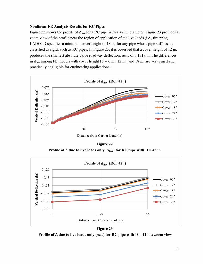
39
Nonlinear FE Analysis Results for RC Pipes
Figure 22 shows the profile of ∆live for a RC pipe with a 42 in. diameter. Figure 23 provides a
zoom view of the profile near the region of application of the live loads (i.e., tire print).
LADOTD specifies a minimum cover height of 18 in. for any pipe whose pipe stiffness is
classified as rigid, such as RC pipes. In Figure 23, it is observed that a cover height of 12 in.
produces the smallest absolute value roadway deflection, live, of 0.1318 in. The differences
in ∆live among FE models with cover height Hc = 6 in., 12 in., and 18 in. are very small and
practically negligible for engineering applications.
Figure 22
Profile of due to live loads only (live) for RC pipe with D = 42 in.
Figure 23
Profile of due to live loads only (live) for RC pipe with D = 42 in.: zoom view
-0.135
-0.125
-0.115
-0.105
-0.095
-0.085
-0.075
0 39 78 117
Ver
tica
l Def
lect
ion
(in
)
Distance from Corner Load (in)
Profile of live (RC: 42")
Cover: 06"
Cover: 12"
Cover: 18"
Cover: 24"
Cover: 30"
-0.134
-0.133
-0.132
-0.131
-0.13
-0.129
0 1.75 3.5
Ver
tica
l Def
lect
ion
(in
)
Distance from Corner Load (in)
Profile of live (RC: 42")
Cover: 06"
Cover: 12"
Cover: 18"
Cover: 24"
Cover: 30"

40
Figure 24 shows the profile of the plastic deformation at the road surface for a 42-in.
diameter RC pipe. An optimal cover height of 18 in. is needed for minimum inelastic
deflection. The plastic deformations are very small, occur almost exclusively in the soil, and
are mainly due to the soil cover self-weight. In Figure 24, it is observed that the data line for
the 12-in. cover intersects the data lines for the 18- and 24-in. covers. The reason for this
phenomenon is that, at the specific cover of 12-in. for a 42-in. diameter RC pipe, the plastic
deformation induced by the live loads is larger than the one produced by the gravity loads.
Figure 24
Profile of due to plastic deformation (inelastic) for RC pipe with D = 42 in.
Figure 25 shows the radius change for a RC pipe with a 42 in. diameter due to live loads
only. As expected, the radius change due to live loads only decreases for increasing cover
height. The observed radius changes are very small for all FE models considered, and the
differences in radius change computed for FE models with different cover heights are almost
negligible. For the considered soil-pipe FE model, ∆live decreases in absolute value by
0.17%, i.e., from 0.1320 in. for Hc = 18 in. (recommended cover height) to 0.1318 in. for Hc
= 12 in. (optimal cover height). This change is practically negligible for application purposes.
For the same FE models, ∆R,live increases by 11.61%.
-0.00005
-0.00004
-0.00003
-0.00002
-0.00001
0
0.00001
0 39 78 117
Ver
tica
l Def
lect
ion
(in
)
Distance from Corner Load (in)
Profile of inelastic (RC: 42")
Cover: 12"
Cover: 18"
Cover: 24"
Cover: 30"
Cover: 36"

41
Figure 25
Comparison of R due to live loads only (R,live) for RC pipe with D = 42 in.
Figure 26 shows the profile of ∆live for a RC pipe with a 60 in. diameter. Figure 27 provides a
zoom view of the profile near the region of application of the live loads. Similarly to the case
of a 42 in. diameter RC pipe, LADOTD specifies a minimum cover height of 18 in. It is
observed that a cover height of 30 in. generates a minimum absolute value roadway
deflection of 0.1379 in. In addition, the profile of ∆live for Hc = 24 in. and 30 in. almost
coincide.
Figure 26
Profile of due to live loads only (live) for RC pipe with D = 60 in.
-0.01
-0.005
0
0.005
0.01
0 45 90 135 180
Rad
ial D
efle
ctio
n (
in)
Theta (°)
Comparison of R,live (RC: 42")
Cover: 18"
Cover: 24"
Cover: 30"
Cover: 36"
Cover: 42"
-0.139
-0.129
-0.119
-0.109
-0.099
-0.089
-0.079
-0.069
0 48 96 144
Ver
tica
l Def
lect
ion
(in
)
Distance from Corner Load (in)
Profile of live(RC: 60")
Cover: 18"
Cover: 24"
Cover: 30"
Cover: 36"
Cover: 42"

42
Figure 27
Profile of due to live loads only (live) for RC pipe with D = 60 in.: zoom view
Figure 28 shows the plastic deformation at the road surface, inelastic, for a 60-in. diameter RC
pipe. An optimal cover height of 24 in. is needed for minimum plastic deformation. Also in
this case, the plastic deformations are very small and affect mainly the soil. Again, the profile
of inelastic corresponding to Hc = 12 in. differs significantly from the profile of inelastic for
larger values of Hc.
Figure 28
Profile of due to plastic deformation (inelastic) for RC pipe with D = 60 in.
Figure 29 shows the radius change due to live loads only, R,live, for a 60-in. diameter RC
pipe. The radius change observed in Figure 29 is very small and slightly decreases for
-0.1385
-0.138
-0.1375
-0.137
-0.1365
-0.136
0 1.75 3.5
Ver
tica
l Def
lect
ion
(in
)
Distance from Corner Load (in)
Profile of live (RC: 60")
Cover: 18"
Cover: 24"
Cover: 30"
Cover: 36"
Cover: 42"
-0.00035-0.0003
-0.00025-0.0002
-0.00015-0.0001
-0.000050
0.00005
0 48 96 144
Ver
tica
l Def
lect
ion
(in
)
Distance from Corner Load (in)
Profile of inelastic(RC: 60")
Cover: 12"
Cover: 18"
Cover: 24"
Cover: 30"
Cover: 36"

43
increasing cover height. For the FE models corresponding to D = 60 in., ∆live decreases in
absolute value by 0.21%, i.e., from 0.1382 in. for Hc = 18 in. to 0.1379 in. for Hc = 30 in.
This change is practically negligible for application purposes. For the same FE models, ∆R,live
decreases by 15.7%.
Figure 29
Comparison of R due to live loads only (R,live) for RC pipe with D = 60 in.
Similar results as the ones presented in detail for the RC pipes were also obtained for the
pipes of other materials. For a more concise exposition, only the zoom views of the profile of
live are shown in the following sections, while the conclusive discussion of the results is
based on all results obtained.
Nonlinear FE Analysis Results for Steel Pipes
Figure 30 shows the profile of live for a 42-in. diameter corrugated steel pipe. For corrugated
steel pipes, LADOTD specifies a minimum cover height of 24 in. It is observed that a cover
height of 30 in. results in a minimum absolute value surface deflection of 0.1357 in. This
deflection is slightly higher than the one observed for an RC pipe of the same diameter. In
addition, the difference in live observed between the models with minimum recommended
and optimal cover heights is very small.
The profile of live for a 60-in. diameter corrugated steel pipe is shown in Figure 31. A
minimum cover height of 24 in. is suggested by LADOTD also for this case. It is observed
that a cover height of 60 in. produces a minimum absolute value of live of 0.1427 in. Also in
this case, the live corresponding to the optimal cover is slightly higher than for an RC pipe of
-0.0125
-0.0075
-0.0025
0.0025
0.0075
0.0125
0 45 90 135 180
Rad
ial D
efle
ctio
n (
in)
Theta (°)
Comparison of R,live (RC: 60")
Cover: 18"
Cover: 24"
Cover: 30"
Cover: 36"
Cover: 42"
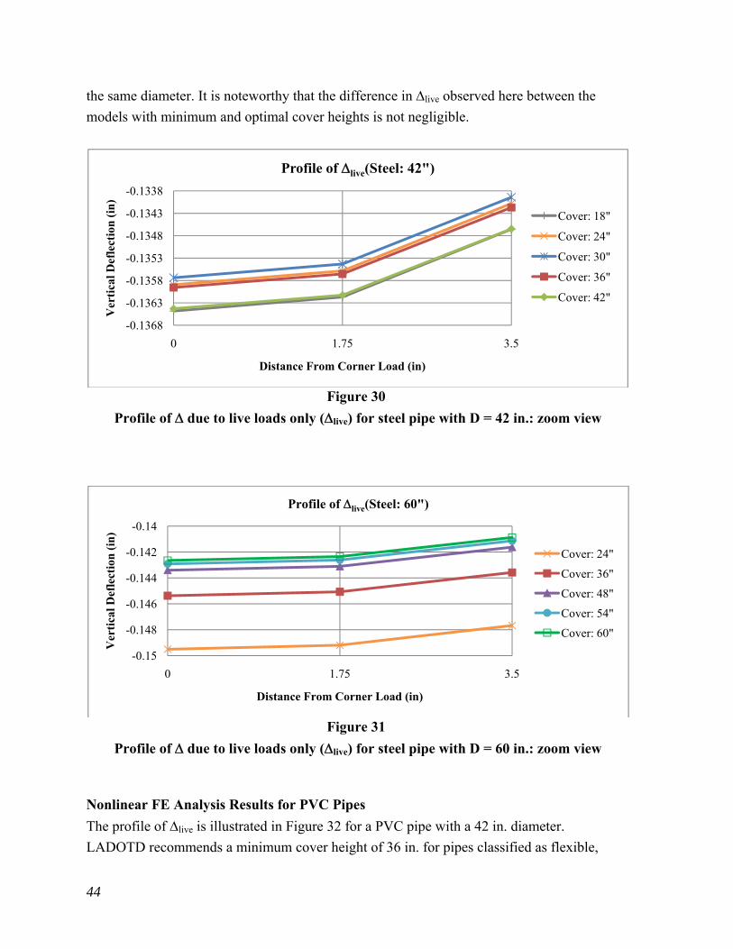
44
the same diameter. It is noteworthy that the difference in live observed here between the
models with minimum and optimal cover heights is not negligible.
Figure 30
Profile of due to live loads only (live) for steel pipe with D = 42 in.: zoom view
Figure 31
Profile of due to live loads only (live) for steel pipe with D = 60 in.: zoom view
Nonlinear FE Analysis Results for PVC Pipes
The profile of live is illustrated in Figure 32 for a PVC pipe with a 42 in. diameter.
LADOTD recommends a minimum cover height of 36 in. for pipes classified as flexible,
-0.1368
-0.1363
-0.1358
-0.1353
-0.1348
-0.1343
-0.1338
0 1.75 3.5
Ver
tica
l Def
lect
ion
(in
)
Distance From Corner Load (in)
Profile of live(Steel: 42")
Cover: 18"
Cover: 24"
Cover: 30"
Cover: 36"
Cover: 42"
-0.15
-0.148
-0.146
-0.144
-0.142
-0.14
0 1.75 3.5
Ver
tica
l Def
lect
ion
(in
)
Distance From Corner Load (in)
Profile of live(Steel: 60")
Cover: 24"
Cover: 36"
Cover: 48"
Cover: 54"
Cover: 60"

45
such as PVC pipes. Minimum roadway deflection is achieved by using an optimal cover
height of 30 in. for a 42-in. PVC pipe. The difference in live observed between the models
with minimum recommended and optimal cover heights is practically negligible in this case.
Figure 32
Profile of due to live loads only (live) for PVC pipe with D = 42 in.: zoom view
Figure 33
Profile of due to live loads only (live) for PVC pipe with D = 60 in.: zoom view
Figure 33 shows the profile of live for a 60-in. diameter PVC pipe. LADOTD recommends a
minimum cover height of 36 in. for all PVC pipes, without differentiation due to the pipe
diameter. A cover height of 60 in. produces a minimum absolute road surface deflection of
0.1433 in. Comparing the results presented in Figure 30 and Figure 31 with the results shown
-0.1378
-0.1373
-0.1368
-0.1363
-0.1358
-0.1353
-0.1348
0 1.75 3.5
Ver
tica
l Def
lect
ion
(in
)
Distance From Corner Load (in)
Profile of live(PVC: 42")
Cover: 18"
Cover: 24"
Cover: 30"
Cover: 36"
Cover: 42"
-0.147
-0.146
-0.145
-0.144
-0.143
-0.142
-0.141
0 1.75 3.5
Ver
tica
l Def
lect
ion
(in
)
Distance From Corner Load (in)
Profile of live(PVC: 60")
Cover: 36"
Cover: 42"
Cover: 48"
Cover: 54"
Cover: 60"

46
in Figure 32 and Figure 33, respectively, it is observed that the minimum absolute values of
live obtained for steel PVC pipes with the same diameter are very similar. At these particular
cover heights, both the steel and PVC pipes are performing almost identically.
Nonlinear FE Analysis Results for HDPE Pipes
Figure 34 shows the profile of live for an HPDE pipe with a 42 in. diameter. LADOTD
specifies a minimum cover height of 36 in. for any pipe classified as flexible, such as HDPE
pipes. It is observed that a cover height of 30 in. produces a minimum absolute value of live
equal to 0.1406 in. However, the difference in live observed here between the models with
minimum recommended and optimal cover heights is practically negligible.
Figure 34
Profile of due to live loads only (live) for HDPE pipe with D = 42 in.: zoom view
The live profile for a 60-in. diameter HDPE pipe is shown in Figure 35. With a pipe stiffness
classified as flexible, a minimum cover height of 36 in. is specified by LADOTD. The
minimum absolute value of live for a 60-in. HDPE pipe is obtained by using an optimal
cover height of 60 in. It is observed that the HDPE pipes are the most flexible pipes among
the materials considered, even when the optimal cover heights are used.
-0.1415
-0.141
-0.1405
-0.14
-0.1395
-0.139
-0.1385
0 1.75 3.5
Ver
tica
l Def
lect
ion
(in
)
Distance From Corner Load (in)
Profile of live (HDPE: 42")
Cover: 18"
Cover: 24"
Cover: 30"
Cover: 36"
Cover: 42"

47
Figure 35
Profile of due to live loads only (live) for HDPE pipe with D = 60 in.: zoom view
Comparison of Deflections for FE Models with Optimal Hc vs. Minimum Hc
Figure 36
Comparison of profile of due to live loads only (live) for all pipes
with D = 42 in.: zoom view
The profiles of live are shown in Figure 36 for all 42-in. diameter pipes of different
materials, including the results for both minimum recommended and optimal cover heights.
The minimum values of cover heights recommended by LADOTD are as follows: 18 in. for
RC, 24 in. for steel, and 36 in. for PVC and HDPE. It is observed than, for all pipes with D =
42 in., the differences in live between the two corresponding models (i.e., with minimum
recommended and optimal cover height for the same material) are negligible.
-0.15
-0.149
-0.148
-0.147
-0.146
-0.145
0 1.75 3.5
Ver
tica
l Def
lect
ion
(in
)
Distance From Corner Load (in)
Profile of live (HDPE: 60")
Cover: 36"
Cover: 42"
Cover: 48"
Cover: 54"
Cover: 60"
-0.142
-0.14
-0.138
-0.136
-0.134
-0.132
-0.13
-0.128
0 1.75 3.5
Ver
tica
l Def
lect
ion
(in
)
Distance From Corner Load (in)
Comparison of Profile of live (42" Pipe)RC (Cover: 12")
RC (Cover: 18")
Steel (Cover: 24")
Steel (Cover: 30")
PVC (Cover: 30")
PVC (Cover: 36")
HDPE (Cover: 30")
HDPE (Cover: 36")

48
Figure 37
Comparison of profile of due to live loads only (live) for all pipes
with D = 60 in.: zoom view
Figure 37 shows the profile of live for all 60-in. diameter pipes of different materials,
including the results for both minimum recommended and optimal cover heights. The
minimum cover heights recommended by LADOTD are the same as for 42-in. diameter pipes
of the same material, i.e., the recommended values of Hc are independent on the pipe
diameter. Comparing the results presented in Figure 36 and Figure 37, it is observed that the
changes in live due to use of an optimal versus minimum cover height of the 60-in. FE
models are much greater for pipes with D = 60 in. than for pipes with D = 42 in.
Table 4 Summary of optimal Hc vs. LADOTD minimum Hc
Pipe Material
D (in.)
LA DOTD Minimum
Hc (in.)
live Optimal Hc (in.)
inelastic Optimal Hc (in.)
R,live Optimal Hc (in.)
R,inelastic Optimal Hc (in.)
RC 42 18 12 18 42 24 RC 60 18 30 24 42 24
Steel 42 24 30 42 60 42 Steel 60 24 60 60 60 60 PVC 42 36 30 18 60 18 PVC 60 36 60 48 60 42
HDPE 42 36 30 48 60 18 HDPE 60 36 60 60 60 60
-0.151
-0.146
-0.141
-0.136
0 1.75 3.5Ver
tica
l Def
lect
ion
(in
)
Distance From Corner Load (in)
Comparison of the Profile of live (60" Pipe)RC (Cover: 18")
RC (Cover: 30")
Steel (Cover: 24")
Steel (Cover: 60")
PVC (Cover: 36")
PVC (Cover: 60")
HDPE (Cover: 36")
HDPE (Cover: 60")

49
Table 4 summarizes LADOTD suggested minimum cover heights and the optimal cover
heights obtained from the results of the nonlinear FE analyses corresponding to the four
different performance measures considered in this study, i.e., (1) live, (2) inelastic, (3) R,live,
and (4) R,inelastic. Hereinafter, the optimal cover height corresponding to the minimum
absolute value of live is considered as the reference value for Hc.
Table 5 compares the performance measures obtained using nonlinear FE models with the
optimal cover height and with LADOTD minimum cover height. The same results are
presented in terms of percentage changes of the performance measures in Table 6. The
optimal cover height is taken as the height of cover, for a particular pipe, corresponding to
which live is minimized in absolute value. In some cases, in order to minimize the road
surface deflection, the radius change may be negatively impacted. For example, to achieve a
minimum absolute live for a 4- in. diameter RC pipe, a cover height of 12 in. is needed
instead of the minimum of 18 in. By doing so, the absolute road surface deflection is
decreased by approximately 0.17% while R,live is increased by 11.61%. It is observed that,
when the optimal cover height is less than the minimum cover height, R,live always
increases. However, when the optimal cover height is greater than the recommended
minimum cover height, the road surface deflection is minimized and the radius change
becomes smaller.
Table 5 Comparison of variation in live and R,live when using optimal Hc vs. LADOTD
minimum Hc
Pipe Material
D (in.)
LA DOTD Minimum
Hc (in.)
Optimal Hc (in.)
∆live (in.) ∆R,live (in.)
Minimum Hc
Optimal Hc
Minimum Hc
Optimal Hc
RC 42 18 12 -0.1320 -0.1318 -0.0074 -0.0083 RC 60 18 30 -0.1382 -0.1379 -0.0101 -0.0085
Steel 42 24 30 -0.1359 -0.1357 -0.0145 -0.0135 Steel 60 24 60 -0.1495 -0.1427 -0.0229 -0.0153 PVC 42 36 30 -0.1369 -0.1368 -0.0136 -0.0143 PVC 60 36 60 -0.1460 -0.1433 -0.0190 -0.0153
HDPE 42 36 30 -0.1408 -0.1406 -0.0204 -0.0210 HDPE 60 36 60 -0.1498 -0.1471 -0.0269 -0.0234

50
Table 6 Comparison of variation of and R when using optimal Hc vs. LADOTD minimum Hc
Pipe Material D
(in.)
LA DOTD Minimum
Hc (in.)
Optimal Hc (in.)
∆live Change
(%)
∆inelastic Change
(%)
∆R,live
Change (%)
∆R,inelastic
Change (%)
RC 42 18 12 -0.17 16.67 11.61 23.08 RC 60 18 30 -0.21 6.33 -15.70 -21.23
Steel 42 24 30 -0.11 -10.79 -6.97 -4.61 Steel 60 24 60 -4.59 -52.48 -33.40 -35.90 PVC 42 36 30 -0.11 -28.21 5.50 -31.03 PVC 60 36 60 -1.87 -5.62 -19.44 7.71
HDPE 42 36 30 -0.13 0.40 2.79 -3.76 HDPE 60 36 60 -1.83 -17.36 -13.21 -12.59
The reinforced concrete (RC) pipe is very rigid when compared to pipes of other materials
and, thus, presents a deflection smaller than pipes with the same diameter and made of other
materials. It is observed in Table 5 that the radius change is much smaller for the RC pipes
when compared to different material pipes with the same diameter. This smaller deflection is
also attributed to the high stiffness of the RC pipe. It is noteworthy that a small deformation
is essential when dealing with concrete pipes. If a large deflection were to occur, cracks
could then form. According to Watkins, the maximum allowable crack width for concrete
pipes is 0.01 in [4]. Fractured conduits can become unstable and the cracks can allow for the
fluid in the pipes to escape into the surrounding soil.
For the nonlinear FE model of the soil-pipe system corresponding to a 42-in. diameter RC
pipe and optimal cover height of 12 in., live decreases in absolute value by 0.17%, when
compared to the FE model corresponding to the recommended cover height of 18 in, i.e.,
from 0.1320 in for Hc = 18 in. to 0.1318 in. for Hc = 12 in. This change is practically
negligible for application purposes. For the same FE models, the maximum absolute value of
R,live decreases by 11.61%. Similar observations can be made for all other pipes as well. As
expected, the performance of the pipes in terms of deformations and road surface deflections
slightly improves when using pipes made of HDPE, PVC, steel, and RC (best performer).
When a buried pipe deflects, the diameter change varies along the circumference of the pipe.
The maximum diameter change is usually found along the vertical direction. Figure 38a
illustrates the total deflections of the pipe in the loaded FE model compared to the unloaded
pipe, while Figure 38b shows the relative deflections of the deformed pipe compared to its
undeformed configuration. The pipe diameter change along the vertical direction is obtained

51
by taking the difference between the deflection at the pipe crest, top, and the deflection at the
bottom, bottom. These deflections are shown in Table 7. The original pipe diameter, deflected
pipe diameter, and pipe diameter changes are shown in Table 8.
Table 7 Displacements at the pipe’s crest and bottom, top and bottom, due to both gravity and
live loads
Pipe Material
D (in.)
LA DOTD minimum Hc (in.)
δtop (in.) δbottom (in.)
RC 42 18 -0.2759 -0.2537 RC 60 18 -0.3359 -0.3038
Steel 42 24 -0.2920 -0.2444 Steel 60 24 -0.3976 -0.3172 PVC 42 36 -0.3178 -0.2631 PVC 60 36 -0.4301 -0.3479
HDPE 42 36 -0.3274 -0.2417 HDPE 60 36 -0.440 -0.3136
Figure 38 Comparison of undeformed and deformed pipe shape: (a) total deflections of the FE
model, and (b) relative deflection of the pipe ring with respect to the undeformed pipe

52
Table 8 Comparison of diameter changes due to both gravity and live loads
Pipe Material
D (in.)
LADOTD minimum Hc (in.)
Deformed Diameter
(in.)
Diameter Change
(in.)
Diameter Change
(%)
Allowable Diameter
Change (%)
Safety Factor
RC 42 18 41.9778 -0.0222 0.0530 0.33 6.23 RC 60 18 59.9680 -0.0320 0.0534 0.20 3.75
Steel 42 24 41.9524 -0.0476 0.1132 5.0 44.17 Steel 60 24 59.9196 -0.0804 0.1340 5.0 37.31 PVC 42 36 41.9453 -0.0547 0.1303 5.0 38.37 PVC 60 36 59.9178 -0.0822 0.1370 5.0 36.50
HDPE 42 36 41.9143 -0.0857 0.2040 5.0 24.51 HDPE 60 36 59.8734 -0.1266 0.2110 5.0 23.70
It is crucial that, for each specific pipe material, the diameter change does not exceed a
specified allowable diameter change, usually expressed as a percentage variation of the
diameter. Since steel, PVC, and HDPE pipes are extremely flexible when compared to RC
pipes, the allowable diameter change for these pipes is much larger than that of RC pipes.
Allowable diameter changes are as follows: 0.33% for RC with D = 42 in. and 0.2% for RC
with D = 60 in. [4], 5% for steel [18], 5% for PVC [11], and 5% for HDPE [12]. The values
for the concrete pipes were obtained from the formula presented in Watkins (2000), d = w / t,
in which d = allowable ring deflection in percentage, w = maximum allowable crack width
that is assumed to equal 0.01 in, and t = pipe wall thickness in inches. It is noteworthy that,
for both PVC and HDPE pipes, an allowable diameter change value equal to 7.5% is
suggested in [18].
The diameter change can be used to define a performance criterion for the pipe. This
performance criterion can be expressed in terms of a safety factor defined as the ratio
between the allowable diameter change and the diameter change obtained from the nonlinear
FE analysis, all quantities being expressed as percentages. Table 8 compares the diameter
change for each nonlinear FE model due to both gravity and live loads with the
corresponding allowable diameter change. The FE models considered here for the soil-pipe
systems have cover heights equal to the minimum values recommended by LADOTD.
Table 8 also provides the safety factor for diameter change for all considered FE models. It is
observed that all pipes are within their individual allowable ranges for diameter change and
that the diameter changes obtained from the nonlinear FE analysis are significantly smaller
than the allowable diameter changes. The performance of the pipes in terms of diameter
changes, due to both gravity and live loads, improves when using pipes made of RC, HDPE,
PVC, and steel, which achieve the best performance in terms of diameter change.

53
CONCLUSIONS
This study analyzed the effects of geometric and mechanical parameters that characterize and
affect the soil-pipe interaction system of buried pipe installations located under
roads/highways. The analysis focused on the combinations of pipe materials and sizes,
natural soil mechanical properties, and road conditions typically encountered in Southern
Louisiana. The drainage pipes or culverts installed as part of a roadway project are
considered as holistic systems that include not only the pipes and their mechanical properties
as determined by materials, geometry, and manufacturing procedures, but also the natural
soil and the trench into which the pipe is placed, constructed, and expected to perform.
The first phase of the research employs linear elastic FE analysis to explore a wide range of
values for numerous geometric and mechanical parameters. The parameters considered
included: (1) excavation (trench) width, (2) fill cover height, (3) bedding height, (4)
mechanical properties of the natural soil surrounding the trench, (5) mechanical properties
and grade of compaction of the fill material, (6) mechanical properties and grade of
compaction of the bedding material, (7) pipe material (RC, steel, PVC, and HDPE), (8)
mechanical and geometric properties of the pipe, (9) material (concrete or asphalt) and
geometry of the roadway pavement and its sub-pavement, and (10) importance of the road
facility. This parametric study consisted of about 25,000 FE analyses and provides pertinent
information about the sensitivity of the performance of the buried pipe installations. This
information is also used to evaluate the conditions under which pipes made of different
materials can perform similarly and, thus, can be used as alternative design solutions.
The sensitivity study based on simplified linear elastic FE analysis showed that the
performance of all soil-pipe systems improves for increasing trench excavation width smaller
than 2D in which D denotes the pipe diameter. This performance improvement is more
significant for flexible pipes and/or yielding natural soil, while this improvement is small for
rigid pipes and stiff natural soil. For trench widths larger than 2D, the performance
improvement is usually very small. The performance of the soil-pipe system significantly
improves for increasing values of Hc for all pipes, even if at a less than linear rate. Thus, for
each pipe, it is possible to find an optimal cover height, Hc, beyond which the performance
improvement of the soil-pipe system is negligible. It was found that the use of stiff bedding
material can cause a significant stress concentration at the bottom of the pipe. The bedding
thickness and bedding material stiffness should be decided in order to ensure that the bedding
of the pipe is stable. This bedding must be able to redistribute as uniformly as possible the
stresses transferred from the pipe and the loading acting above the pipe.

54
It was found that the natural soil stiffness also significantly influences the performance of
soil-pipe systems. The natural soil properties considered in this study were based on typical
conditions encountered in Southern Louisiana, where very soft clay is common. In addition,
it was found that the performance of soil-pipe systems in terms of live depends crucially on
the type of road surface. A stiffer road pavement distributes the stresses produced by the live
loads more uniformly over a much larger area of soil. Thus, an increase in stiffness of the
road pavement significantly decreases the magnitude of the stresses that are transferred to the
pipe through the road pavement, the sub-pavement, and the trench cover. As a consequence,
live also decreases substantially.
Linear elastic FE analysis is also used to determine the appropriate dimensions for a 3-D FE
model of buried pipe installation. This model dimension sensitivity study suggests that, in
order to obtain results insensitive to model dimensions, the FE model needs to include a
region of natural soil surrounding the trench with the dimensions of one trench width in the
horizontal direction and half a trench width in the vertical direction. In the direction of the
pipe axis, a thickness of 24 in. sufficiently models 3-D effects.
The second phase of the research, based on advanced nonlinear FE analysis, evaluates four
different performance measures for buried pipe installations with pipes of different materials
(RC, steel, PVC, and HDPE) and different internal diameters (42 in. and 60 in.), i.e., (1) road
surface deflection due to live loads only, live, (2) plastic road surface deflection, inelastic, (3)
radial deformation due to live loads only, R,live, and (4) plastic radial deformation, R,inelastic.
The main results of this research phase are the optimal values of the cover height for the
trench fill material corresponding to each performance measure considered. It was found that
the optimal cover heights are very close to the minimum cover heights recommended by
LADOTD for 42-in. diameter pipes. In addition, the observed differences in the performance
measures are practically negligible for application purposes. However, for pipes with
diameters equal to 60 in., the differences in performance between optimal and minimum
recommended cover heights are significant. This observation suggests that the value of the
minimum recommended cover height should be expressed as a function of the pipe diameter
in order to ensure a homogeneous level of performance. When considering the optimal cover
height, the performance of the pipes in terms of road surface deflections, live, slightly
improves when using pipes made of HDPE, PVC, steel, and RC (best performer) when the
same natural soil conditions and road pavement type are considered. When considering the
minimum recommended cover height, the performance of the pipes in terms of diameter
changes, due to both gravity and live loads, improves when using pipes made of RC, HDPE,
PVC, and steel (best performer).

55
The research results confirm that the performance of the soil-structure interaction system
constituted by the pipe, the trench backfill, and the natural soil surrounding the trench
depends significantly not only on the pipe material and stiffness, but also on geometric
parameters defining the trench in which the pipe is installed. Minimum requirements for
these geometric parameters can be established to obtain equivalent performance of different
pipe systems under similar design conditions.

56

57
RECOMMENDATIONS
This research focused on soil conditions typical of Southern Louisiana. The results of this
research, when integrated with appropriate experimental data and field experience, can be
used as guidance in establishing guidelines for the alternate selection and application of
typical highway drainage products, such as pipes and culverts.
Based on the results obtained in this research, the following specific recommendations are
made for implementation:
1) The minimum cover height should be expressed as a function of the pipe diameter.
2) For flexible and semi-flexible pipes, the minimum trench width should be equal to twice
the pipe diameter, while for rigid pipes, a minimum trench width equal to the pipe
diameter + 3 ft. is sufficient.
3) Different minimum requirements can be made for yielding and stiff soils. In the absence
of specific data from in-situ tests, the more demanding requirements for yielding soil
should be followed in favor of safety.
4) Different minimum requirements can be made for different road pavements with more
demanding requirements for more flexible road pavements.
Further research is also recommended in order to determine the effects on the performance of
buried pipe installation of (1) the removal of trench installation walls, (2) the long-term
behavior and the fatigue behavior of soil-pipe systems, (3) the fluctuation of the water level
in the soil near the buried pipes, and (4) uncertainty in pipes, trench filling material, and
natural soil.


59
ACRONYMS, ABBREVIATIONS, & SYMBOLS
2-D Two Dimensional
3-D Three Dimensional
AASHTO American Association of State Highway and Transportation Officials
ADS Advanced Drainage Systems Inc.
AISC American Institute of Steel Construction
AutoCAD Auto Computer Aided Design
C3D4 4-noded linear tetrahedron
C3D6 6-noded triangular prism
C3D8I 8-noded linear brick with incompatible modes
CANDE Culvert Analysis and Design
CDP Concrete Damaged Plasticity
DOF Degrees of Freedom
DOT Department of Transportation
FE Finite Element
FEA Finite Element Analysis
FHWA Federal Highway Administration
H20 AASHTO Standard H-type 20 Ton Vehicle
HDPE High Density Polyethylene
LADOTD Louisiana Department of Transportation
LE Linear Elastic
LRFD Load Resistance Factor Design
LTRC Louisiana Transportation Research Center
PVC Polyvinyl Chloride
RC Reinforced Concrete
SPIDA Soil-Pipe Interaction and Design Analysis
SSI Soil-Structure Interaction
ft. feet
hrs hours
in. inch(es)
kips kilo pounds
ksi kilo pounds per square inch
lb/ft3 pounds per cubic foot
mins minutes
cb bedding material cohesion

60
cf fill material cohesion
cs natural soil cohesion
d allowable diameter change percentage
D pipe diameter
deflection
inelastic maximum dip depth at road surface due to plastic deformation
live maximum dip depth at road surface due to live loads only
max maximum elastic deformation at road surface due to both gravity and live loads
R,inelastic maximum radial deformation due to plastic deformation
R,live maximum radial deformation due to live loads only
σ maximum stress increment
δtop deflection at the pipe crest
δbottom deflection at the pipe bottom
E Young’s modulus
Eb bedding material stiffness
Ef fill material stiffness
Es natural soil stiffness
Esp sub-pavement stiffness
Hb bedding height
Hc fill cover height
Hp road pavement thickness
Hsp sub-pavement thickness
I moment of inertia
% percentage
φ friction angle
φb bedding material friction angle
φf fill material friction angle
φs natural soil friction angle
θ reference angle for radial deformation
t pipe thickness
w allowable crack width
W trench excavation width
σmax maximum stress reached in the pipe due to both gravity and live loads
σy yield strength
∑ summation

61
REFERENCES
1. Jeyapalan, J. K. and Hamida, H. B. “Comparison of German to Marston Design Methods.” ASCE Journal of Transportation Engineering, Vol. 114, No. 4, 1988, pp. 420-434.
2. Burns, J. C. “Experimental Investigation of Shear Capacity of Precast Reinforced Concrete Box Culverts.” M.S. Thesis. The University of Texas at Arlington, Arlington, TX, 2009.
3. Katona, M. G., Smith, J. M., Odello, R. S., and Allgood, J. R. “CANDE - A Modern Approach for the Structural Design and Analysis of Buried Culverts.” Report No. FHWA-RD-77-5, U.S. Naval Civil Engineering Lab, Port Hueneme, CA, 1976.
4. Watkins, R. K., and Anderson L. R. Structural Mechanics of Buried Pipes. CRC Press LLC, Boca Raton, FL, 2000.
5. Slatter, G. “Suggested Bedding Factors of Controlled Low-Strength Material for Concrete Pipe.” Proceedings, ASCE International Conference on Pipeline Engineering and Construction, July 13-16, 2003, Baltimore, MD. Editor: Najafi M., Publisher: American Society of Civil Engineering, New York, NY, 2003, pp. 1086–1095.
6. CSI. SAP2000 Application Programming Interface Documentation. Version 11. Computers & Structure, Inc., Berkeley, CA, 2007.
7. AASHTO. LRFD Bridge Design Specifications. American Association of State and Highway Transportation Officials. Washington, D.C., 2007.
8. ABAQUS. Version 6.8 Documentation. Dassault Systemes Simulia Corp., Providence, RI, 2008.
9. AASHTO M 170. Standard Specification for Reinforced Concrete Culvert, Storm Drain, and Sewer Pipe. American Association of State and Highway Transportation Officials. Washington, D.C., 2007.
10. AASHTO M 36. Standard Specification for Corrugated Steel Pipe, Metallic-Coated for Sewers and Drains. American Association of State and Highway Transportation Officials. Washington, D.C., 2007.
11. AASHTO M 278. Standard Specification for Class PS46 Poly (Vinyl Chloride) (PVC) Pipe. American Association of State and Highway Transportation Officials. Washington, D.C., 2007.

62
12. AASHTO M 294. Standard Specification for Corrugated Polyethylene Pipe, 300 to
1500 mm Diameter. American Association of State and Highway Transportation Officials. Washington, D.C., 2007.
13. Kararam, A. “Nonlinear Finite Element-Based Investigation of the Effect of Bedding Thickness on Underground Pipe.” M.S. Thesis. The University of Texas at Arlington, Arlington, TX, 2006.
14. Ibrahimbegovic, A. (2009). Nonlinear Solid Mechanics: Theoretical Formulations and Finite Element Solution Methods. Series: Solid Mechanics and Its Applications, Vol. 160, Springer-Verlag, New York, NY, 2009.
15. Jankowiak, T., and Lodygowski, T. “Identification of Parameters of Concrete Damage Plasticity Constitutive Model.” Foundations of Civil and Environmental Engineering, Vol. 6, 2005, pp. 53-69.
16. Budhu, M. Soil Mechanics and Foundations. 1st Edition. John Wiley and Sons, Inc., Hoboken, NJ, 2000.
17. AISC. Steel Construction Manual. 13th Edition. American Institute of Steel Construction, Inc., Chicago, IL, 2005.
18. Moser, A. P. Buried Pipe Design. 2nd Edition. McGraw-Hill, New York, NY, 2001.

63
APPENDIX A
Nonlinear FE Results for Overall Comparisons
Figure 39 Profile of live for RC pipe with D = 42 in.
Figure 40 Profile of live for RC pipe with D = 42 in.: zoom view
-0.135
-0.125
-0.115
-0.105
-0.095
-0.085
-0.075
0 39 78 117
Ver
tica
l Def
lect
ion
(in
)
Distance from Corner Load (in)
Profile of live (RC: 42")
Cover: 06"
Cover: 12"
Cover: 18"
Cover: 24"
Cover: 30"
Cover: 36"
Cover: 42"
-0.135
-0.134
-0.133
-0.132
-0.131
-0.13
-0.129
0 1.75 3.5
Ver
tica
l Def
lect
ion
(in
)
Distance from Corner Load (in)
Profile of live (RC: 42")
Cover: 06"
Cover: 12"
Cover: 18"
Cover: 24"
Cover: 30"
Cover: 36"
Cover: 42"

64
Figure 41 Profile of inelastic for RC pipe with D = 42 in.
Figure 42 Profile of inelastic for RC pipe with D = 42 in.: zoom view
-0.00007-0.00006-0.00005-0.00004-0.00003-0.00002-0.00001
00.000010.000020.00003
0 39 78 117
Ver
tica
l Def
lect
ion
(in
)
Distance from Corner Load (in)
Profile of inelastic (RC: 42")
Cover: 06"
Cover: 12"
Cover: 18"
Cover: 24"
Cover: 30"
Cover: 36"
Cover: 42"
-7E-05
-6E-05
-5E-05
-4E-05
-3E-05
-2E-05
0 1.75 3.5
Ver
tica
l Def
lect
ion
(in
)
Distance from Corner Load (in)
Profile of inelastic (RC: 42")
Cover: 06"
Cover: 12"
Cover: 18"
Cover: 24"
Cover: 30"
Cover: 36"
Cover: 42"

65
Figure 43 Comparison of R,live for RC pipe with D = 42 in.
Figure 44 Comparison of R,live for RC pipe with D = 42 in.: zoom view
-0.01
-0.005
0
0.005
0.01
0 45 90 135 180
Rad
ial D
efle
ctio
n (
in)
Theta (°)
Comparison of R,live (RC: 42")
Cover: 06"
Cover: 12"
Cover: 18"
Cover: 24"
Cover: 30"
Cover: 36"
Cover: 42"
-0.01
-0.009
-0.008
-0.007
-0.006
-0.005
0 2.61 5.22 7.83 10.44
Rad
ial D
efle
ctio
n (
in)
Theta (°)
Comparison of R,live (RC: 42")
Cover: 06"
Cover: 12"
Cover: 18"
Cover: 24"
Cover: 30"
Cover: 36"
Cover: 42"

66
Figure 45 Comparison of R,inelastic for RC pipe with D = 42 in.
Figure 46 Comparison of R,inelastic for RC pipe with D = 42 in.: zoom view
-8E-05
-6E-05
-4E-05
-2E-05
1.6E-18
2E-05
4E-05
6E-05
0 45 90 135 180
Rad
ial D
efle
ctio
n (
in)
Theta (°)
Comparison of R,inelastic (RC: 42")
Cover: 06"
Cover: 12"
Cover: 18"
Cover: 24"
Cover: 30"
Cover: 36"
Cover: 42"
-7E-05
-6E-05
-5E-05
-4E-05
-3E-05
-2E-05
-1E-05
0 2.61 5.22 7.83 10.44
Rad
ial D
efle
ctio
n (
in)
Theta (°)
Comparison of R,inelastic (RC: 42")
Cover: 06"
Cover: 12"
Cover: 18"
Cover: 24"
Cover: 30"
Cover: 36"
Cover: 42"

67
Figure 47 Profile of live for RC pipe with D = 60 in.
Figure 48 Profile of live for RC pipe with D = 60 in.: zoom view
-0.139
-0.129
-0.119
-0.109
-0.099
-0.089
-0.079
-0.069
0 48 96 144
Ver
tica
l Def
lect
ion
(in
)
Distance from Corner Load (in)
Profile of live (RC: 60")
Cover: 06"
Cover: 12"
Cover: 18"
Cover: 24"
Cover: 30"
Cover: 36"
Cover: 42"
-0.14
-0.1395
-0.139
-0.1385
-0.138
-0.1375
-0.137
-0.1365
-0.136
0 1.166 2.332 3.498
Ver
tica
l Def
lect
ion
(in
)
Distance from Corner Load (in)
Profile of live (RC: 60")
Cover: 06"
Cover: 12"
Cover: 18"
Cover: 24"
Cover: 30"
Cover: 36"
Cover: 42"

68
Figure 49 Profile of inelastic for RC pipe with D = 60 in.
Figure 50 Profile of inelastic for RC pipe with D = 60 in.: zoom view
-0.0005
-0.0004
-0.0003
-0.0002
-0.0001
0
0.0001
0.0002
0 48 96 144
Ver
tica
l Def
lect
ion
(in
)
Distance from Corner Load (in)
Profile of inelastic (RC: 60")
Cover: 06"
Cover: 12"
Cover: 18"
Cover: 24"
Cover: 30"
Cover: 36"
Cover: 42"
-0.0004-0.00038-0.00036-0.00034-0.00032
-0.0003-0.00028-0.00026-0.00024-0.00022
-0.0002
0 1.166 2.332 3.498
Ver
tica
l Def
lect
ion
(in
)
Distance from Corner Load (in)
Profile of inelastic (RC: 60")
Cover: 06"
Cover: 12"
Cover: 18"
Cover: 24"
Cover: 30"
Cover: 36"
Cover: 42"

69
Figure 51 Comparison of R,live for RC pipe with D = 60 in.
Figure 52 Comparison of R,live for RC pipe with D = 60 in.: zoom view
-0.015
-0.01
-0.005
0
0.005
0.01
0.015
0 45 90 135 180
Rad
ial D
efle
ctio
n (
in)
Theta (°)
Comparison of R,live (RC: 60")
Cover: 06"
Cover: 12"
Cover: 18"
Cover: 24"
Cover: 30"
Cover: 36"
Cover: 42"
-0.013
-0.012
-0.011
-0.01
-0.009
-0.008
-0.007
-0.006
0 1.855 3.71 5.565 7.42 9.275 11.13
Rad
ial D
efle
ctio
n (
in)
Theta (°)
Comparison of R,live (RC: 60")
Cover: 06"Cover: 12"Cover: 18"Cover: 24"Cover: 30"Cover: 36"Cover: 42"

70
Figure 53 Comparison of R,inelastic for RC pipe with D = 60 in.
Figure 54 Comparison of R,inelastic for RC pipe with D = 60 in.: zoom view
-0.00025-0.0002
-0.00015-0.0001
-0.000050
0.000050.0001
0.000150.0002
0.00025
0 45 90 135 180
Rad
ial D
efle
ctio
n (
in)
Theta (°)
Comparison of R,inelastic (RC: 60")
Cover: 06"
Cover: 12"
Cover: 18"
Cover: 24"
Cover: 30"
Cover: 36"
Cover: 42"
-0.0002
-0.00018
-0.00016
-0.00014
-0.00012
-0.0001
-8E-05
-6E-05
-4E-05
0 1.855 3.71 5.565 7.42 9.275 11.13
Rad
ial D
efle
ctio
n (
in)
Theta (°)
Comparison of R,inelastic (RC: 60")
Cover: 06"
Cover: 12"
Cover: 18"
Cover: 24"
Cover: 30"
Cover: 36"
Cover: 42"

71
Figure 55 Profile of live for steel pipe with D = 42 in.
Figure 56 Profile of live for steel pipe with D = 42 in.: zoom view
-0.14
-0.13
-0.12
-0.11
-0.1
-0.09
-0.08
-0.07
-0.06
0 42 84 126
Ver
tica
l Def
lect
ion
(in
)
Distance From Corner Load (in)
Profile of live (Steel: 42")
Cover: 12"
Cover: 18"
Cover: 24"
Cover: 30"
Cover: 36"
Cover: 42"
-0.138
-0.137
-0.136
-0.135
-0.134
-0.133
0 1.75 3.5
Ver
tica
l Def
lect
ion
(in
)
Distance From Corner Load (in)
Profile of live (Steel: 42")
Cover: 12"
Cover: 18"
Cover: 24"
Cover: 30"
Cover: 36"
Cover: 42"

72
Figure 57 Profile of inelastic for steel pipe with D = 42 in.
Figure 58 Profile of inelastic for steel pipe with D = 42 in.: zoom view
-0.0016-0.0014-0.0012-0.001
-0.0008-0.0006-0.0004-0.0002
00.00020.00040.0006
0 42 84 126
Ver
tica
l Def
lect
ion
(in
)
Distance From Corner Load (in)
Profile of inelastic (Steel: 42")
Cover: 12"
Cover: 18"
Cover: 24"
Cover: 30"
Cover: 36"
Cover: 42"
-0.0016
-0.0015
-0.0014
-0.0013
-0.0012
-0.0011
-0.001
-0.0009
-0.0008
0 1.75 3.5
Ver
tica
l Def
lect
ion
(in
)
Distance From Corner Load (in)
Profile of inelastic (Steel: 42")
Cover: 12"
Cover: 18"
Cover: 24"
Cover: 30"
Cover: 36"
Cover: 42"

73
Figure 59 Comparison of R,live for steel pipe with D = 42 in.
Figure 60 Comparison of R,live for steel pipe with D = 42 in.: zoom view
-0.02
-0.015
-0.01
-0.005
0
0.005
0.01
0.015
0.02
0 45 90 135 180
Rad
ial D
efle
ctio
n (
in)
Theta (°)
Comparison of R,live (Steel: 42")
Cover: 12"
Cover: 18"
Cover: 24"
Cover: 30"
Cover: 36"
Cover: 42"
-0.018
-0.017
-0.016
-0.015
-0.014
-0.013
-0.012
-0.011
0 4.09 8.18 12.27
Rad
ial D
efle
ctio
n (
in)
Theta (°)
Comparison of R,live (Steel: 42")
Cover: 12"
Cover: 18"
Cover: 24"
Cover: 30"
Cover: 36"
Cover: 42"

74
Figure 61 Comparison of R,inelastic for steel pipe with D = 42 in.
Figure 62 Comparison of R,inelastic for steel pipe with D = 42 in.: zoom view
-0.002
-0.0015
-0.001
-0.0005
0
0.0005
0.001
0.0015
0.002
0 45 90 135 180
Rad
ial D
efle
ctio
n (
in)
Theta (°)
Comparison of R,inelastic (Steel: 42")
Cover: 12"
Cover: 18"
Cover: 24"
Cover: 30"
Cover: 36"
Cover: 42"
-0.0015
-0.0014
-0.0013
-0.0012
-0.0011
-0.001
0 4.09 8.18 12.27
Rad
ial D
efle
ctio
n (
in)
Theta (°)
Comparison of R,inelastic (Steel: 42")
Cover: 12"
Cover: 18"
Cover: 24"
Cover: 30"
Cover: 36"
Cover: 42"

75
Figure 63 Profile of live for steel pipe with D = 60 in.
Figure 64 Profile of live for steel pipe with D = 60 in.: zoom view
-0.18-0.16-0.14-0.12
-0.1-0.08-0.06-0.04-0.02
0
0 60 120 180
Ver
tica
l Def
lect
ion
(in
)
Distance From Corner Load (in)
Profile of live (Steel: 60")
Cover: 12"
Cover: 18"
Cover: 24"
Cover: 30"
Cover: 36"
Cover: 42"
Cover: 48"
Cover: 54"
Cover: 60"
-0.158-0.156-0.154-0.152-0.15
-0.148-0.146-0.144-0.142-0.14
0 1.75 3.5
Ver
tica
l Def
lect
ion
(in
)
Distance From Corner Load (in)
Profile of live (Steel: 60")
Cover: 12"
Cover: 18"
Cover: 24"
Cover: 30"
Cover: 36"
Cover: 42"
Cover: 48"
Cover: 54"
Cover: 60"

76
Figure 65 Profile of inelastic for steel pipe with D = 60 in.
Figure 66 Profile of inelastic for steel pipe with D = 60 in.: zoom view
-0.005
-0.004
-0.003
-0.002
-0.001
0
0.001
0.002
0 60 120 180
Ver
tica
l Def
lect
ion
(in
)
Distance From Corner Load (in)
Profile of inelastic (Steel: 60")
Cover: 12"
Cover: 18"
Cover: 24"
Cover: 30"
Cover: 36"
Cover: 42"
Cover: 48"
Cover: 54"
Cover: 60"
-0.0045
-0.004
-0.0035
-0.003
-0.0025
-0.002
-0.0015
0 1.75 3.5
Ver
tica
l Def
lect
ion
(in
)
Distance From Corner Load (in)
Profile of inelastic (Steel: 60")
Cover: 12"
Cover: 18"
Cover: 24"
Cover: 30"
Cover: 36"
Cover: 42"
Cover: 48"
Cover: 54"
Cover: 60"

77
Figure 67 Comparison of R,live for steel pipe with D = 60 in.
Figure 68 Comparison of R,live for steel pipe with D = 60 in.: zoom view
-0.04
-0.03
-0.02
-0.01
0
0.01
0.02
0.03
0 45 90 135 180
Rad
ial D
efle
ctio
n (
in)
Theta (°)
Comparison of R,live (Steel: 60")
Cover: 12"
Cover: 18"
Cover: 24"
Cover: 30"
Cover: 36"
Cover: 42"
Cover: 48"
Cover: 54"
Cover: 60"
-0.03
-0.028
-0.026
-0.024
-0.022
-0.02
-0.018
-0.016
-0.014
0 2.857 5.714 8.571 11.428
Rad
ial D
efle
ctio
n (
in)
Theta (°)
Comparison of R,live (Steel: 60")
Cover: 12"
Cover: 18"
Cover: 24"
Cover: 30"
Cover: 36"
Cover: 42"
Cover: 48"
Cover: 54"
Cover: 60"

78
Figure 69 Comparison of R,inelastic for steel pipe with D = 60 in.
Figure 70 Comparison of R,inelastic for steel pipe with D = 60 in.: zoom view
-0.005-0.004-0.003-0.002-0.001
00.0010.0020.0030.004
0 45 90 135 180
Rad
ial D
efle
ctio
n (
in)
Theta (°)
Comparison of R,inelastic(Steel: 60")
Cover: 12"
Cover: 18"
Cover: 24"
Cover: 30"
Cover: 36"
Cover: 42"
Cover: 48"
Cover: 54"
Cover: 60"
-0.004
-0.0035
-0.003
-0.0025
-0.002
0 2.857 5.714 8.571 11.428
Rad
ial D
efle
ctio
n (
in)
Theta (°)
Comparison of R,inelastic (Steel: 60")
Cover: 12"
Cover: 18"
Cover: 24"
Cover: 30"
Cover: 36"
Cover: 42"
Cover: 48"
Cover: 54"
Cover: 60"

79
Figure 71 Profile of live for PVC pipe with D = 42 in.
Figure 72 Profile of live for PVC pipe with D = 42 in.: zoom view
-0.14
-0.13
-0.12
-0.11
-0.1
-0.09
-0.08
0 42 84 126
Ver
tica
l Def
lect
ion
(in
)
Distance From Corner Load (in)
Profile of live (PVC: 42")
Cover: 18"
Cover: 24"
Cover: 30"
Cover: 36"
Cover: 42"
Cover: 48"
Cover: 54"
Cover: 60"
-0.14
-0.139
-0.138
-0.137
-0.136
-0.135
-0.134
0 1.75 3.5
Ver
tica
l Def
lect
ion
(in
)
Distance From Corner Load (in)
Profile of live (PVC: 42")
Cover: 18"
Cover: 24"
Cover: 30"
Cover: 36"
Cover: 42"
Cover: 48"
Cover: 54"
Cover: 60"

80
Figure 73 Profile of inelastic for PVC pipe with D = 42 in.
Figure 74 Profile of inelastic for PVC pipe with D = 42 in.: zoom view
-0.00012
-0.0001
-0.00008
-0.00006
-0.00004
-0.00002
0
0 42 84 126
Ver
tica
l Def
lect
ion
(in
)
Distance From Corner Load (in)
Profile of inelastic (PVC: 42")
Cover: 18"
Cover: 24"
Cover: 30"
Cover: 36"
Cover: 42"
Cover: 48"
Cover: 54"
Cover: 60"
-0.00011
-9E-05
-7E-05
-5E-05
-3E-05
-1E-05
0 1.75 3.5
Ver
tica
l Def
lect
ion
(in
)
Distance From Corner Load (in)
Profile of inelastic (PVC: 42") Cover: 18"
Cover: 24"
Cover: 30"
Cover: 36"
Cover: 42"
Cover: 48"
Cover: 54"
Cover: 60"

81
Figure 75 Comparison of R,live for PVC pipe with D = 42 in.
Figure 76 Comparison of R,live for PVC pipe with D = 42 in.: zoom view
-0.02
-0.015
-0.01
-0.005
0
0.005
0.01
0.015
0 45 90 135 180
Rad
ial D
efle
ctio
n (
in)
Theta (°)
Comparison of R,live (PVC: 42")
Cover: 18"
Cover: 24"
Cover: 30"
Cover: 36"
Cover: 42"
Cover: 48"
Cover: 54"
Cover: 60"
-0.017
-0.016
-0.015
-0.014
-0.013
-0.012
-0.011
0 5.4545 10.909
Rad
ial D
efle
ctio
n (
in)
Theta (°)
Comparison of R,live (PVC: 42")
Cover: 18"
Cover: 24"
Cover: 30"
Cover: 36"
Cover: 42"
Cover: 48"
Cover: 54"
Cover: 60"

82
Figure 77 Comparison of R,inelastic for PVC pipe with D = 42 in.
Figure 78 Comparison of R,inelastic for PVC pipe with D = 42 in.: zoom view
-0.00015
-0.0001
-0.00005
0
0.00005
0.0001
0.00015
0.0002
0 45 90 135 180
Rad
ial D
efle
ctio
n (
in)
Theta (°)
Comparison of R,inelastic (PVC: 42")
Cover: 18"
Cover: 24"
Cover: 30"
Cover: 36"
Cover: 42"
Cover: 48"
Cover: 54"
Cover: 60"
-0.00013
-0.00011
-9E-05
-7E-05
-5E-05
-3E-05
-1E-05
0 5.4545 10.909
Rad
ial D
efle
ctio
n (
in)
Theta (°)
Comparison of R,inelastic (PVC: 42") Cover: 18"
Cover: 24"
Cover: 30"
Cover: 36"
Cover: 42"
Cover: 48"
Cover: 54"
Cover: 60"
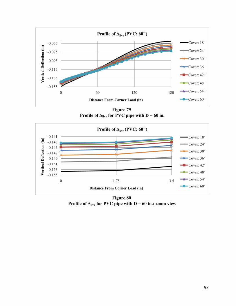
83
Figure 79 Profile of live for PVC pipe with D = 60 in.
Figure 80 Profile of live for PVC pipe with D = 60 in.: zoom view
-0.155
-0.135
-0.115
-0.095
-0.075
-0.055
0 60 120 180
Ver
tica
l Def
lect
ion
(in
)
Distance From Corner Load (in)
Profile of live (PVC: 60")
Cover: 18"
Cover: 24"
Cover: 30"
Cover: 36"
Cover: 42"
Cover: 48"
Cover: 54"
Cover: 60"
-0.155
-0.153
-0.151
-0.149
-0.147
-0.145
-0.143
-0.141
0 1.75 3.5
Ver
tica
l Def
lect
ion
(in
)
Distance From Corner Load (in)
Profile of live (PVC: 60")
Cover: 18"
Cover: 24"
Cover: 30"
Cover: 36"
Cover: 42"
Cover: 48"
Cover: 54"
Cover: 60"

84
Figure 81 Profile of inelastic for PVC pipe with D = 60 in.
Figure 82 Profile of inelastic for PVC pipe with D = 60 in.: zoom view
-0.0008
-0.0006
-0.0004
-0.0002
-3E-18
0.0002
0 60 120 180
Ver
tica
l Def
lect
ion
(in
)
Distance From Corner Load (in)
Profile of inelastic (PVC: 60")
Cover: 18"
Cover: 24"
Cover: 30"
Cover: 36"
Cover: 42"
Cover: 48"
Cover: 54"
Cover: 60"
-0.00078
-0.00073
-0.00068
-0.00063
-0.00058
-0.00053
-0.00048
0 1.75 3.5
Ver
tica
l Def
lect
ion
(in
)
Distance From Corner Load (in)
Profile of inelastic (PVC: 60")
Cover: 18"
Cover: 24"
Cover: 30"
Cover: 36"
Cover: 42"
Cover: 48"
Cover: 54"
Cover: 60"

85
Figure 83 Comparison of R,live for PVC pipe with D = 60 in.
Figure 84 Comparison of R,live for PVC pipe with D = 60 in.: zoom view
-0.03
-0.02
-0.01
0
0.01
0.02
0.03
0 45 90 135 180
Rad
ial D
efle
ctio
n (
in)
Theta (°)
Comparison of R,live (PVC: 60")
Cover: 18"
Cover: 24"
Cover: 30"
Cover: 36"
Cover: 42"
Cover: 48"
Cover: 54"
Cover: 60"
-0.026
-0.024
-0.022
-0.02
-0.018
-0.016
-0.014
0 3.66 7.32 10.98
Rad
ial D
efle
ctio
n (
in)
Theta (°)
Comparison of R,live (PVC: 60") Cover: 18"
Cover: 24"
Cover: 30"
Cover: 36"
Cover: 42"
Cover: 48"
Cover: 54"
Cover: 60"

86
Figure 85 Comparison of R,inelastic for PVC pipe with D = 60 in.
Figure 86 Comparison of R,inelastic for PVC pipe with D = 60 in.: zoom view
-0.0008
-0.0006
-0.0004
-0.0002
0
0.0002
0.0004
0.0006
0.0008
0 45 90 135 180
Rad
ial D
efle
ctio
n (
in)
Theta (°)
Comparison of R,inelastic (PVC: 60")
Cover: 18"
Cover: 24"
Cover: 30"
Cover: 36"
Cover: 42"
Cover: 48"
Cover: 54"
Cover: 60"
-0.00072
-0.00067
-0.00062
-0.00057
-0.00052
0 3.66 7.32 10.98
Rad
ial D
efle
ctio
n (
in)
Theta (°)
Comparison of R,inelastic (PVC: 60")
Cover: 18"
Cover: 24"
Cover: 30"
Cover: 36"
Cover: 42"
Cover: 48"
Cover: 54"
Cover: 60"

87
Figure 87 Profile of live for HDPE pipe with D = 42 in.
Figure 88 Profile of live for HDPE pipe with D = 42 in.: zoom view
-0.15
-0.14
-0.13
-0.12
-0.11
-0.1
-0.09
-0.08
0 42 84 126
Ver
tica
l Def
lect
ion
(in
)
Distance From Corner Load (in)
Profile of live (HDPE: 42")
Cover: 18"
Cover: 24"
Cover: 30"
Cover: 36"
Cover: 42"
Cover: 48"
Cover: 54"
Cover: 60"
-0.144
-0.143
-0.142
-0.141
-0.14
-0.139
-0.138
0 1.75 3.5
Ver
tica
l Def
lect
ion
(in
)
Distance From Corner Load (in)
Profile of live (HDPE: 42")
Cover: 18"
Cover: 24"
Cover: 30"
Cover: 36"
Cover: 42"
Cover: 48"
Cover: 54"
Cover: 60"

88
Figure 89 Profile of inelastic for HDPE pipe with D = 42 in.
Figure 90 Profile of inelastic for HDPE pipe with D = 42 in.: zoom view
-0.0006
-0.0005
-0.0004
-0.0003
-0.0002
-0.0001
0 42 84 126
Ver
tica
l Def
lect
ion
(in
)
Distance From Corner Load (in)
Profile of inelastic (HDPE: 42")
Cover: 18"
Cover: 24"
Cover: 30"
Cover: 36"
Cover: 42"
Cover: 48"
Cover: 54"
Cover: 60"
-0.00056
-0.00054
-0.00052
-0.0005
-0.00048
-0.00046
0 1.75 3.5
Ver
tica
l Def
lect
ion
(in
)
Distance From Corner Load (in)
Profile of inelastic (HDPE: 42")
Cover: 18"
Cover: 24"
Cover: 30"
Cover: 36"
Cover: 42"
Cover: 48"
Cover: 54"
Cover: 60"

89
Figure 91 Comparison of R,live for HDPE pipe with D = 42 in.
Figure 92 Comparison of R,live for HDPE pipe with D = 42 in.: zoom view
-0.025
-0.02
-0.015
-0.01
-0.005
0
0.005
0.01
0.015
0 45 90 135 180
Rad
ial D
efle
ctio
n (
in)
Theta (°)
Comparison of R,live (HDPE: 42")
Cover: 18"
Cover: 24"
Cover: 30"
Cover: 36"
Cover: 42"
Cover: 48"
Cover: 54"
Cover: 60"
-0.0232
-0.0222
-0.0212
-0.0202
-0.0192
-0.0182
0 4.09 8.18 12.27
Rad
ial D
efle
ctio
n (
in)
Theta (°)
Comparison of R,live (HDPE: 42")
Cover: 18"
Cover: 24"
Cover: 30"
Cover: 36"
Cover: 42"
Cover: 48"
Cover: 54"
Cover: 60"

90
Figure 93 Comparison of R,inelastic for HDPE pipe with D = 42 in.
Figure 94 Comparison of R,inelastic for HDPE pipe with D = 42 in.: zoom view
-0.001-0.0008-0.0006-0.0004-0.0002
00.00020.00040.00060.00080.001
0 45 90 135 180
Rad
ial D
efle
ctio
n (
in)
Theta (°)
Comparison of R,inelastic (HDPE: 42")
Cover: 18"
Cover: 24"
Cover: 30"
Cover: 36"
Cover: 42"
Cover: 48"
Cover: 54"
Cover: 60"
-0.00095
-0.0009
-0.00085
-0.0008
-0.00075
0 4.09 8.18 12.27
Rad
ial D
efle
ctio
n (
in)
Theta (°)
Comparison of R,inelastic (HDPE: 42")
Cover: 18"
Cover: 24"
Cover: 30"
Cover: 36"
Cover: 42"
Cover: 48"
Cover: 54"
Cover: 60"

91
Figure 95 Profile of live for HDPE pipe with D = 60 in.
Figure 96 Profile of live for HDPE pipe with D = 60 in.: zoom view
-0.16
-0.14
-0.12
-0.1
-0.08
-0.06
-0.04
0 60 120 180
Ver
tica
l Def
lect
ion
(in
)
Distance From Corner Load (in)
Profile of live (HDPE: 60")
Cover: 18"
Cover: 24"
Cover: 30"
Cover: 36"
Cover: 42"
Cover: 48"
Cover: 54"
Cover: 60"
-0.16-0.158-0.156-0.154-0.152
-0.15-0.148-0.146-0.144
0 1.75 3.5
Ver
tica
l Def
lect
ion
(in
)
Distance From Corner Load (in)
Profile of live (HDPE: 60")
Cover: 18"
Cover: 24"
Cover: 30"
Cover: 36"
Cover: 42"
Cover: 48"
Cover: 54"
Cover: 60"

92
Figure 97 Profile of inelastic for HDPE pipe with D = 60 in.
Figure 98 Profile of inelastic for HDPE pipe with D = 60 in.: zoom view
-0.002
-0.0015
-0.001
-0.0005
-1E-17
0.0005
0 60 120 180
Ver
tica
l Def
lect
ion
(in
)
Distance From Corner Load (in)
Profile of inelastic (HDPE: 60")
Cover: 18"
Cover: 24"
Cover: 30"
Cover: 36"
Cover: 42"
Cover: 48"
Cover: 54"
Cover: 60"
-0.002
-0.0018
-0.0016
-0.0014
-0.0012
-0.001
0 1.75 3.5
Ver
tica
l Def
lect
ion
(in
)
Distance From Corner Load (in)
Profile of inelastic (HDPE: 60")
Cover: 18"
Cover: 24"
Cover: 30"
Cover: 36"
Cover: 42"
Cover: 48"
Cover: 54"
Cover: 60"

93
Figure 99 Comparison of R,live for HDPE pipe with D = 60 in.
Figure 100 Comparison of R,live for HDPE pipe with D = 60 in.: zoom view
-0.035
-0.025
-0.015
-0.005
0.005
0.015
0.025
0 45 90 135 180
Rad
ial D
efle
ctio
n (
in)
Theta (°)
Comparison of R,live (HDPE: 60")
Cover: 18"
Cover: 24"
Cover: 30"
Cover: 36"
Cover: 42"
Cover: 48"
Cover: 54"
Cover: 60"
-0.034
-0.032
-0.03
-0.028
-0.026
-0.024
-0.022
-0.02
0 2.814 5.628 8.442 11.256 14.07
Rad
ial D
efle
ctio
n (
in)
Theta (°)
Comparison of R,live (HDPE: 60")
Cover: 18"
Cover: 24"
Cover: 30"
Cover: 36"
Cover: 42"
Cover: 48"
Cover: 54"
Cover: 60"

94
Figure 101 Comparison of R,inelastic for HDPE pipe with D = 60 in.
Figure 102 Comparison of R,inelastic for HDPE pipe with D = 60 in.: zoom view
-0.003
-0.002
-0.001
-1E-17
0.001
0.002
0 45 90 135 180
Rad
ial D
efle
ctio
n (
in)
Theta (°)
Comparison of R,inelastic (HDPE: 60")
Cover: 18"
Cover: 24"
Cover: 30"
Cover: 36"
Cover: 42"
Cover: 48"
Cover: 54"
Cover: 60"
-0.0028
-0.0026
-0.0024
-0.0022
-0.002
-0.0018
0 2.814 5.628 8.442 11.256 14.07
Rad
ial D
efle
ctio
n (
in)
Theta (°)
Comparison of R,inelastic (HDPE: 60")
Cover: 18"
Cover: 24"
Cover: 30"
Cover: 36"
Cover: 42"
Cover: 48"
Cover: 54"
Cover: 60"
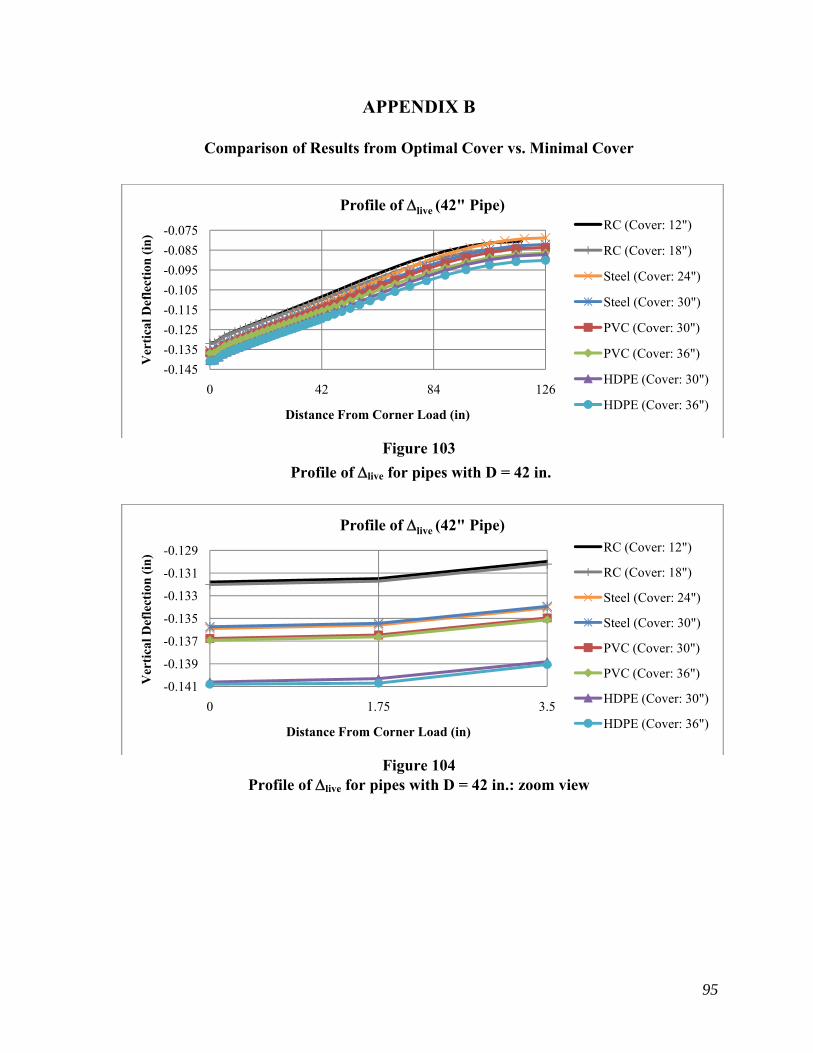
95
APPENDIX B
Comparison of Results from Optimal Cover vs. Minimal Cover
Figure 103
Profile of live for pipes with D = 42 in.
Figure 104 Profile of live for pipes with D = 42 in.: zoom view
-0.145
-0.135
-0.125
-0.115
-0.105
-0.095
-0.085
-0.075
0 42 84 126
Ver
tica
l Def
lect
ion
(in
)
Distance From Corner Load (in)
Profile of live (42" Pipe)RC (Cover: 12")
RC (Cover: 18")
Steel (Cover: 24")
Steel (Cover: 30")
PVC (Cover: 30")
PVC (Cover: 36")
HDPE (Cover: 30")
HDPE (Cover: 36")
-0.141
-0.139
-0.137
-0.135
-0.133
-0.131
-0.129
0 1.75 3.5
Ver
tica
l Def
lect
ion
(in
)
Distance From Corner Load (in)
Profile of live (42" Pipe)RC (Cover: 12")
RC (Cover: 18")
Steel (Cover: 24")
Steel (Cover: 30")
PVC (Cover: 30")
PVC (Cover: 36")
HDPE (Cover: 30")
HDPE (Cover: 36")

96
Figure 105 Profile of inelastic for pipes with D = 42 in.
Figure 106 Comparison of R,live for pipes with D = 42 in.
-0.0012
-0.001
-0.0008
-0.0006
-0.0004
-0.0002
0
0.0002
0 42 84 126
Ver
tica
l Def
lect
ion
(in
)
Distance From Corner Load (in)
Profile of inelastic (42" Pipe)RC (Cover: 12")
RC (Cover: 18")
Steel (Cover: 24")
Steel (Cover: 30")
PVC (Cover: 30")
PVC (Cover: 36")
HDPE (Cover: 30")
HDPE (Cover: 36")
-0.025-0.02
-0.015-0.01
-0.0050
0.0050.01
0.015
0 45 90 135 180
Rad
ial D
efle
ctio
n (
in)
Theta (°)
Comparison of R,live (42" Pipe)
RC (Cover: 12")
RC (Cover: 18")
Steel (Cover: 24")
Steel (Cover: 30")
PVC (Cover: 30")
PVC (Cover: 36")
HDPE (Cover: 30")
HDPE (Cover: 36")

97
Figure 107 Comparison of R,inelastic for pipes with D = 42 in.
Figure 108 Profile of live for pipes with D = 60 in.
-0.0015
-0.001
-0.0005
0
0.0005
0.001
0.0015
0 45 90 135 180
Rad
ial D
efle
ctio
n (
in)
Theta (°)
Comparison of R,inelastic (42" Pipe)
RC (Cover: 12")
RC (Cover: 18")
Steel (Cover: 24")
Steel (Cover: 30")
PVC (Cover: 30")
PVC (Cover: 36")
HDPE (Cover: 30")
HDPE (Cover: 36")
-0.15
-0.13
-0.11
-0.09
-0.07
-0.05
0 60 120 180
Ver
tica
l Def
lect
ion
(in
)
Distance From Corner Load (in)
Profile of live (60" Pipe)RC (Cover: 18")
RC (Cover: 30")
Steel (Cover: 24")
Steel (Cover: 60")
PVC (Cover: 36")
PVC (Cover: 60")
HDPE (Cover: 36")
HDPE (Cover: 60")

98
Figure 109 Profile of live for pipes with D = 60 in.: zoom view
Figure 110 Profile of inelastic for pipes with D = 60 in.
-0.153
-0.148
-0.143
-0.138
-0.133
0 1.75 3.5
Ver
tica
l Def
lect
ion
(in
)
Distance From Corner Load (in)
Profile of live (60" Pipe)
RC (Cover: 18")
RC (Cover: 30")
Steel (Cover: 24")
Steel (Cover: 60")
PVC (Cover: 36")
PVC (Cover: 60")
HDPE (Cover: 36")
HDPE (Cover: 60")
-0.004
-0.003
-0.002
-0.001
-1E-17
0.001
0 60 120 180
Ver
tica
l Def
lect
ion
(in
)
Distance From Corner Load (in)
Profile of inelastic (60" Pipe)
RC (Cover: 18")
RC (Cover: 30")
Steel (Cover: 24")
Steel (Cover: 60")
PVC (Cover: 36")
PVC (Cover: 60")
HDPE (Cover: 36")
HDPE (Cover: 60")

99
Figure 111 Comparison of R,live for pipes with D = 60 in.
Figure 112 Comparison of R,inelastic for pipes with D = 60 in.
-0.03
-0.02
-0.01
0
0.01
0.02
0 45 90 135 180
Rad
ial D
efle
ctio
n (
in)
Theta (°)
Comparison of R,live (60" Pipe)
RC (Cover: 18")
RC (Cover: 30")
Steel (Cover: 24")
Steel (Cover: 60")
PVC (Cover: 36")
PVC (Cover: 60")
HDPE (Cover: 36")
HDPE (Cover: 60")
-0.004-0.003-0.002-0.001
00.0010.0020.0030.004
0 45 90 135 180
Rad
ial D
efle
ctio
n (
in)
Theta (°)
Comparison of R,inelastic (60" Pipe)RC (Cover: 18")
RC (Cover: 30")
Steel (Cover: 24")
Steel (Cover: 60")
PVC (Cover: 36")
PVC (Cover: 60")
HDPE (Cover: 36")
HDPE (Cover: 60")

100
Figure 113 Profile of live for RC pipes
Figure 114 Profile of live for RC pipes: zoom view
-0.139
-0.129
-0.119
-0.109
-0.099
-0.089
-0.079
-0.069
0 48 96 144
Ver
tica
l Def
lect
ion
(in
)
Distance From Corner Load (in)
Profile of live (RC)
D=42" (Cover: 12")
D=42" (Cover: 18")
D=60" (Cover: 18")
D=60" (Cover: 30")
-0.139
-0.137
-0.135
-0.133
-0.131
-0.129
0 1.75 3.5
Ver
tica
l Def
lect
ion
(in
)
Distance From Corner Load (in)
Profile of live (RC)
D=42" (Cover: 12")
D=42" (Cover: 18")
D=60" (Cover: 18")
D=60" (Cover: 30")

101
Figure 115 Comparison of R,live for RC pipes
Figure 116 Profile of live for steel pipes
-0.012
-0.009
-0.006
-0.003
3.1E-17
0.003
0.006
0.009
0.012
0 45 90 135 180
Rad
ial D
efle
ctio
n (
in)
Theta (°)
Comparison of R,live (RC)
D=42" (Cover:12")
D=42" (Cover: 18")
D=60" (Cover: 18")
D=60" (Cover: 30")
-0.15
-0.13
-0.11
-0.09
-0.07
-0.05
0 60 120 180
Ver
tica
l Def
lect
ion
(in
)
Distance From Corner Load (in)
Profile of live (Steel)
D=42" (Cover: 24")
D=42" (Cover: 30")
D=60" (Cover: 24")
D=60" (Cover: 60")

102
Figure 117 Profile of live for steel pipes: zoom view
Figure 118 Comparison of R,live for steel pipes
-0.15
-0.145
-0.14
-0.135
-0.13
0 1.75 3.5
Ver
tica
l Def
lect
ion
(in
)
Distance From Corner Load (in)
Profile of live (Steel)
D=42" (Cover: 24")
D=42" (Cover: 30")
D=60" (Cover: 24")
D=60" (Cover: 60")
-0.025-0.02
-0.015-0.01
-0.0050
0.0050.01
0.0150.02
0 45 90 135 180
Rad
ial D
efle
ctio
n (
in)
Theta (°)
Comparison of R,live (Steel)
D=42" (Cover: 24")
D=42" (Cover: 30")
D=60" (Cover: 24")
D=60" (Cover: 60")

103
Figure 119 Profile of live for PVC pipes
Figure 120 Profile of live for PVC pipes: zoom view
-0.147
-0.127
-0.107
-0.087
-0.067
-0.047
0 60 120 180
Ver
tica
l Def
lect
ion
(in
)
Distance From Corner Load (in)
Profile of live (PVC)
D=42" (Cover:30")
D=42" (Cover: 36")
D=60" (Cover:36")
D=60" (Cover: 60")
-0.147
-0.145
-0.143
-0.141
-0.139
-0.137
-0.135
0 1.75 3.5
Ver
tica
l Def
lect
ion
(in
)
Distance From Corner Load (in)
Profile of live (PVC)
D=42" (Cover:30")
D=42" (Cover: 36")
D=60" (Cover:36")
D=60" (Cover: 60")

104
Figure 121 Comparison of R,live for PVC pipes
Figure 122 Profile of live for HDPE pipes
-0.02-0.015
-0.01-0.005
00.0050.01
0.0150.02
0 45 90 135 180
Rad
ial D
efle
ctio
n (
in)
Theta (°)
Comparison of R,live (PVC)
D=42" (Cover: 30")
D=42" (Cover: 36")
D=60" (Cover: 36")
D=60" (Cover: 60")
-0.15
-0.13
-0.11
-0.09
-0.07
-0.05
0 60 120 180
Ver
tica
l Def
lect
ion
(in
)
Distance From Corner Load (in)
Profile of live (HDPE)
D=42" (Cover: 30")
D=42" (Cover: 36")
D=60" (Cover: 36")
D=60" (Cover: 60")

105
Figure 123 Profile of live for HDPE pipes: zoom view
Figure 124 Comparison of R,live for HDPE pipes
-0.15
-0.148
-0.146
-0.144
-0.142
-0.14
-0.138
0 1.75 3.5
Ver
tica
l Def
lect
ion
(in
)
Distance From Corner Load (in)
Profile of live (HDPE)
D=42" (Cover: 30")
D=42" (Cover: 36")
D=60" (Cover: 36")
D=60" (Cover: 60")
-0.03
-0.02
-0.01
0
0.01
0.02
0 45 90 135 180
Rad
ial D
efle
ctio
n (
in)
Theta (°)
Comparison of R,live (HDPE)
D=42" (Cover: 30")
D=42" (Cover: 36")
D=60" (Cover: 36")
D=60" (Cover: 60")