LTE radio network deployment design in urban environments ... · LTE radio network deployment...

LTE radio network deployment design in urban

environments under different traffic scenarios

António Bernardo Barreiros de Alcobia

Thesis to obtain the Master of Science Degree in

Electrical and Computer Engineering

Supervisor: Prof. Luís Manuel de Jesus Sousa Correia

Examination Committee

Chairperson: Prof. José Eduardo Charters Ribeiro da Cunha Sanguino

Supervisor: Prof. Luís Manuel de Jesus Sousa Correia

Members of Committee: Prof. António José Castelo Branco Rodrigues

Eng. André Martins

May 2017

iii

To my family

v

Acknowledgements

Acknowledgements

First of all, I would like to thank Prof. Luis M. Correia. It has been an amazing opportunity to develop

this thesis under his supervision, not only for his continuous support and, always, ready assistance, but

mainly for his important advices and friendship. I am grateful for his encouragement and invaluable

guidance throughout this thesis. Also, I would like to thank him for providing me the chance to develop

this work in collaboration with Celfinet, and for the valuable experience of belonging to the GROW

Research Group.

Special acknowledgement is also dedicated to Eng. André Martins, who followed my work from Celfinet’

point of view, and helped me with his prised advices and support during the development of this thesis,

helping me to improve the quality of my work.

I must extend my gratitude to all GROW members, especially my master´s thesis colleagues José Guita,

Hugo Silva and Tiago Monteiro for their friendship and precious advices.

My gratitude is also dedicated to my good old friends and to the good ones I made at IST, André Cabrita,

Ricardo Cabrita, António Mestre, Tomás Monteiro, Bernardo Almeida, and Luis Rodrigues, who were

always by my side and followed my journey from really close, never letting me down, and to all the rest

that were not mentioned, a very special thanks for supporting me during the last years.

Last, but not least, I would like to show all my gratitude to my family, specially to my grandmother, mother

and father for their unconditional love and support, and for all sacrifices that they have done for me, as

without them none of this would have been possible.

vii

Abstract

Abstract

The focus of this thesis was on the dimensioning of LTE radio access networks and the development of

tools for dimensioning purposes. The main purpose is to compute the number of cells needed to cover

a given area, taking a specific traffic profile into account. A model taking coverage and capacity planning

into account was developed, regarding the 800,1800 and 2600 MHz frequency bands, in three different

environments (urban, suburban and rural). The effect of varying parameters regarding user density,

geographical area, frequency band and bandwidth, cell edge target throughput, traffic profile, among

others, was studied in order to understand the impact of these parameters on the number of cells. For

this purpose, a model was implemented, which takes a certain area and user density into consideration

and makes the allocation of resources depending on system coverage and available capacity, replicating

as close as possible the behaviour of a real network. A significant increase in the total number of cells

is verified when the density of users increases. With more users, more resources are needed to fulfil the

coverage and capacity requirements. Results show that, for all scenarios, most of the obtained cells are

limited by capacity. Thus, the variation of service mix and services throughputs has a particular impact

on the required number of cells. The number of urban cells for the voice centric scenario decreases

about 12% over the ROM scenario, whereas, for the scenario with lower throughputs, the number of

urban cells decreases about 41% over the ROM scenario.

Keywords

LTE, Dimensioning, Coverage, Capacity, Number of Cells, Lisbon.

viii

Resumo

Resumo O foco desta tese foi o dimensionamento das redes de acesso de rádio LTE e o desenvolvimento de

ferramentas de dimensionamento. O objetivo principal é calcular o número de células necessárias para

cobrir uma determinada área, tendo em conta um perfil de tráfego específico. Foi desenvolvido um

modelo tendo em conta o planeamento da cobertura e da capacidade, considerando as bandas de

frequências de 800, 1800 e 2600 MHz, em três ambientes diferentes (urbano, suburbano e rural).

Estudou-se o efeito da variação de alguns parâmetros relativos à densidade de utilizadores, área

geográfica, banda de frequência e largura de banda, débito binário requerido no bordo da célula, perfil

de tráfego, entre outros, de forma a compreender o impacto destes parâmetros no número de células.

Para isso, foi implementado um modelo que tem em consideração uma determinada área e uma

determinada densidade de utilizadores e realiza a atribuição de recursos dependendo da cobertura do

sistema e da capacidade disponível, tentando replicar tanto quanto possível, o comportamento de uma

rede real. Verifica-se um aumento no número de células quando a densidade de utilizadores aumenta.

Com mais utilizadores, mais recursos são necessários para cumprir os requisitos de cobertura e

capacidade. Os resultados mostram que, para todos os cenários, a maioria das células obtidas

encontra-se limitada pela capacidade. Assim, a variação da mistura de serviços e dos débitos binários

dos serviços tem um impacto particular no número de células obtidas. O número de células urbanas

para o cenário focado no serviço de voz diminuiu cerca de 12% em relação ao cenário ROM, enquanto

que para o cenário com débito binário menor, o número de células urbanas diminuiu cerca de 41% em

relação ao cenário ROM.

Palavras-chave

LTE, Dimensionamento, Cobertura, Capacidade, Número de Células, Lisboa.

ix

Table of Contents

Table of Contents

Acknowledgements ................................................................................. v

Abstract ................................................................................................. vii

Resumo ................................................................................................ viii

Table of Contents ................................................................................... ix

List of Figures ........................................................................................ xi

List of Tables ......................................................................................... xiii

List of Acronyms .................................................................................. xiv

List of Symbols ..................................................................................... xvii

List of Software ..................................................................................... xx

1 Introduction .................................................................................. 1

1.1 Overview.................................................................................................. 2

1.2 Motivation and Contents .......................................................................... 4

2 Fundamental Concepts and State of the Art ................................. 7

2.1 Network Architecture ............................................................................... 8

2.2 Radio Interface ........................................................................................ 9

2.3 Coverage and Capacity ......................................................................... 14

2.4 Services and Applications...................................................................... 18

2.5 Heterogeneous Networks ...................................................................... 21

2.6 State of the Art ....................................................................................... 24

3 Models and Simulator Description .............................................. 27

3.1 Model Development ............................................................................... 28

3.1.1 Dimensioning Process ......................................................................................... 28

3.1.2 Inputs and Outputs of LTE Dimensioning ............................................................ 29

3.1.3 Coverage Planning .............................................................................................. 30

3.1.4 Capacity Planning ................................................................................................ 34

x

3.1.5 Cellular Planning.................................................................................................. 37

3.2 Model Implementation ........................................................................... 38

3.3 Model Assessment ................................................................................ 42

4 Results Analysis ......................................................................... 45

4.1 Scenarios Description ............................................................................ 46

4.2 Analysis on the Number of Users .......................................................... 54

4.3 Bandwidth and Frequency Band Analysis ............................................. 55

4.4 Analysis on Coverage Percentages ....................................................... 58

4.5 Traffic Profiles Analysis ......................................................................... 59

4.6 Impact of Reference Throughput Analysis ............................................. 64

5 Conclusions ................................................................................ 65

Annex A. SINR versus Throughput..................................................... 71

Annex B. Propagation Models ............................................................ 73

B.1 COST-231 Walfisch-Ikegami Model ...................................................... 74

B.2 Okumura-Hata Model ............................................................................ 76

Annex C Districts ............................................................................... 79

References............................................................................................ 87

xi

List of Figures

List of Figures Figure 1.1 - Global mobile traffic for voice and data, 2015-2021 (extracted from [Eric15a]). ....... 2

Figure 1.2 - Schedule of the 3GPP standards and their commercial deployment (adapted from [HoTo11]) ............................................................................................................. 3

Figure 1.3 - Area chart with the number of global mobile subscriptions for different technologies, 2011-2021 (extracted from [Eric15a]). ................................................................. 4

Figure 2.1. System Architecture for E-UTRAN only Network (extracted from [HoTo11]). ............ 8

Figure 2.2 - Frame Structure type 1 with short CP (extracted from [Share16]). ......................... 11

Figure 2.3 - OFDMA resource allocation in LTE (extracted from [Corr16]). ................................ 12

Figure 2.4 - DL frame structure with normal CP (extracted from [Agil09]). ................................. 13

Figure 2.5 - Example of different carrier frequencies and respective coverage area. ................ 15

Figure 2.6 - Example of interference scenario in LTE-A Network (extracted from [Aldh13]) ...... 16

Figure 2.7- Throughput per RB in DL vs. SINR for different MCS (extracted from [Pire15]). ..... 17

Figure 2.8 – LTE-A Heterogeneous Network (extracted from [JaMa13]). ................................... 22

Figure 2.9 – LTE-A HetNet Multi-Site Carrier Aggregation (extracted from [Ali15]).................... 23

Figure 3.1 - LTE network dimensioning. ...................................................................................... 28

Figure 3.2 - LTE coverage planning. ........................................................................................... 30

Figure 3.3 - UL Link Budget......................................................................................................... 32

Figure 3.4 – Mean (green), outdoor (blue) and indoor radii (red)................................................ 33

Figure 3.5 - Uniform distribution of users. ................................................................................... 34

Figure 3.6 - Capacity planning. ................................................................................................... 37

Figure 3.7 - Simulator Workflow. ................................................................................................. 39

Figure 3.8 – Number of cells versus User density. ..................................................................... 43

Figure 3.9 - Percentage of served users towards the covered ones. ......................................... 44

Figure 3.10 – Cell Radius versus User density. .......................................................................... 44

Figure 4.1 – Reference user density in the Lisbon City and its surrounding areas. ................... 46

Figure 4.2 - Population density of each municipality. .................................................................. 47

Figure 4.3 - BSs positioning in the Lisbon City and surrounding areas (adapted from [Maro15]). ........................................................................................................... 47

Figure 4.4 - List of analysed Input and Output parameters. ........................................................ 51

Figure 4.4 – Division of the reference area into environments (adapted from Google Maps). ... 52

Figure 4.6 – Number of cells for each municipality taking the reference parameters into account. ............................................................................................................. 52

Figure 4.7 - Number of cells per 10 km2 for each environment. .................................................. 53

Figure 4.8 – Average cell radius for each environment. .............................................................. 54

Figure 4.9 – Number of cells per 10 km2 for different scenarios taking users’ density into account. ........................................................................................................................... 55

Figure 4.10 – Number of cells per 10 km2 for different scenarios (reference scenario in darker grey). .................................................................................................................. 57

Figure 4.11 – Number of cells per 10 km2 vs. bandwidths and frequency bands. ...................... 57

Figure 4.12 – Number of cells for each district vs. outdoor and indoor coverage percentages. . 59

Figure 4.13 – Division of urban area into residential (orange) and office (grey) ones (extracted from [Fon16]). .................................................................................................... 60

xii

Figure 4.14 – Number of urban cells per 10 km2, for different service profiles scenarios. .......... 62

Figure 4.15 – Number of urban cells per 10 km2 for each scenario. ........................................... 63

Figure B.1 - Parameters in the COST-231 Walfisch-Ikegami Model........................................... 76

xiii

List of Tables

List of Tables Table 2.1 – LTE FDD frequency bands used in Europe (adapted from [HoTo11]). .................... 10

Table 2.2 - Relationship among bandwidth, number of sub-carriers and of RBs (adapted from [Corr16]). ............................................................................................................ 12

Table 2.3 – UL peak data rates not considering MIMO (extracted from [Alme13]). .................... 17

Table 2.4 - DL peak data rates (extracted from [Alme13]). ......................................................... 18

Table 2.5 - QoS service classes summary, according to 3GPP (adapted from [3GPP15a]). ..... 19

Table 2.6 - QoS parameters for QCI (extracted from [SeTB11])................................................. 20

Table 2.7 - Services characteristics. ........................................................................................... 21

Table 3.1 - List of empirical tests performed to validate the implementation of the coverage model. ........................................................................................................................... 42

Table 3.2 - List of empirical tests performed to validate the implementation of the capacity model. ........................................................................................................................... 43

Table 4.1 – Indoor Mean and Standard Deviation for each frequency band (extracted from [Corr16]). ............................................................................................................ 48

Table 4.2 – Parameters for the reference scenario. .................................................................... 48

Table 4.3 - Simulation Parameters. ............................................................................................. 49

Table 4.4 - Configuration of parameters for the propagations models. ....................................... 50

Table 4.5 - Services characteristics (adapted from [Guit16]) ...................................................... 51

Table 4.6 - Penetration and Usage Ratio for each scenario. ..................................................... 54

Table 4.7 – Maximum radius of a cell for different bands. .......................................................... 56

Table 4.8 – Variation of the cell radius vs. outdoor and indoor coverage percentages. ............. 58

Table 4.9 – Total number of urban cells for different traffic profiles. ........................................... 60

Table 4.10 – Service mix of each user type profile. .................................................................... 61

Table 4.11 – Service mix scenarios. ........................................................................................... 61

Table 4.12 – Throughput values for the studied scenarios. ........................................................ 63

Table C.1 - Lisbon Districts Characteristics. ............................................................................... 80

Table C.2 - AV Districts Characteristics. ..................................................................................... 81

Table C.3 - SMA Districts Characteristics. .................................................................................. 81

Table C.4 - Sintra Districts Characteristics. ................................................................................. 82

Table C.5 - Cascais Districts Characteristics. ............................................................................. 82

Table C.6 - Odivelas Districts Characteristics. ............................................................................ 83

Table C.7 - Amadora Districts Characteristics. ........................................................................... 83

Table C.8 - Mafra Districts Characteristics. ................................................................................. 84

Table C.9 - Loures Districts Characteristics. ............................................................................... 84

Table C.10 - Oeiras Districts Characteristics. ............................................................................. 85

Table C.11 - VFX Districts Characteristics. ................................................................................. 85

xiv

List of Acronyms

List of Acronyms 16-QAM Four bits per symbol Quadrature Amplitude Modulation

3G Third Generation

3GPP Third Generation Partnership Project

4G Fourth Generation

64-QAM Six bits per symbol Quadrature Amplitude Modulation

ABS Almost Blank Sub-frames

AMBR Aggregated Maximum Bit rate

AMC Adaptive Modulation and Coding

ANACOM Autoridade Nacional de Comunicações

BER Bit Error Rate

BLER Block Error Rate

BS Base Station

CA Carrier Aggregation

CC Component Carriers

CoMP Coordinated Multi-Point

CP Cyclic Prefix

CRE Cell Range Extension

CSG Closed Subscriber Group

DL Downlink

EDGE Enhanced Data Rates for GSM Evolution

EIRP Effective Isotropic Radiated Power

eICIC Enhanced Inter Cell Interference Coordination

eNB Evolved Node B

EPC Evolved Packet Core

EPS Evolved Packet System

E-UTRAN Evolved UMTS Terrestrial Radio Access Network

FB Frequency Band

feICIC Further Enhanced Inter Cell Interference Coordination

FDD Frequency Division Duplex

FTP File Transfer Protocol

GBR Guaranteed Bit Rate

GSM Global System for Mobile

GSM1800 GSM 1 800 MHz frequency band

HetNet Heterogeneous Network

xv

HSPA High Speed Packet data Access

HSS Home Subscription Server

ICI Inter Cell Interference

ICIC Inter Cell Interference Coordination

IP Internet Protocol

ISI Inter Symbol Interference

LTE Long Term Evolution

LTE1800 LTE 1 800 MHz frequency band

LTE-A Long Term Evolution Advanced

MAPL Maximum Allowed Path Loss

M2M Machine-to-Machine

MBR Maximum Bit Rate

MIMO Multiple-Input Multiple-Output

OFDM Orthogonal Frequency-Division Multiplexing

OFDMA Orthogonal Frequency-Division Multiple Access

P2P Peer-to-Peer

PBCH Physical Broadcast Channel

Pcell Primary Cell

PCRF Policy Control and Charging Rules Function

PDCCH Physical Downlink Control Channel

PDN Packet Data Network

PDSCH Physical Downlink Shared Control Channel

P-GW Packet Data Network Gateway

PRACH Physical Random Access Channel

P-SS Primary Synchronisation Signal

PUCCH Physical Uplink Control Channel

PUSCC Physical Uplink Shared Control Channel

QCI QoS Class Identifier

QoS Quality of Service

QPSK Quadrature Phase Shift Keying

RAN Radio Access Network

RB Resource Block

RE Resource Element

RLB Radio Link Budget

ROM Residential, Office and Mix scenario

SAE System Architecture Evolution

Scell Secondary Cell

SC-FDMA Single Carrier Frequency-Division Multiple Access

S-GW Serving Gateway

SINR Signal to Interference Noise Ratio

xvi

SMS Short Message Service

SNR Signal-to-Noise Ratio

S-SS Secondary Synchronisation Signal

TDD Time Division Duplex

TMA Tower Mounted Amplifier

TTI Transmission Time Interval

UE User Equipment

UL Uplink

UMTS Universal Mobile Telecommunications System

VoIP Voice over IP

VoLTE Voice over LTE

WCDMA Wideband Code Division Multiple Access

WWW World Wide Web

xvii

List of Symbols

List of Symbols

� Path loss exponent

�� Average power decay

η User density

�� Cell capacity ratio

�� Time transmission interval

ɣ SINR requirement for the uplink or downlink traffic channel

�� SINR

��,� Available SINR from �� link in each single sub-carrier (k)

σ Standard deviation

� Street orientation angle

∆��,��%�� Average indoor slow fading margin

∆��,��%�� Average outdoor slow fading margin

�� Site coverage area

�� Target area

��,� Fading channel gain for donor cell

��,� Fading channel gain for neighbouring cell

�� Bandwidth of one RB

�� Extended Okumura-Hata model variable

� Distance between the BS and the UE

��,� Distance from user to donor base station

��,� Distance from user to neighbouring cells

� Frequency band

�� Noise figure

�� Gain of the receiving antenna

�� Gain of the transmitting antenna

�� Tower Mounted Amplifier gain

�� Diversity Gain

�� Buildings height

ℎ� Effective height of BS antenna

ℎ� User equipment height

�� Okumura-Hata model variable

�� Interference Margin

�� Okumura-Hata model correction factor

xviii

�� Free space propagation path loss

�� Losses in the cable between the transmitter and the antenna

�� Path loss coming from the COST-231 Walfisch-Ikegami or Okumura-Hata model

��,�� Average path loss coming from indoor penetration

��,�� Maximum path loss

��,�� Average path loss coming from the propagation models

��,�� Total path loss

�� Loss in the UE for the DL, or loss in the cable between the transmitter and the antenna for the UL

�� Attenuation due to diffraction from the last rooftop to the UE

�� Attenuation due to propagation from the BS to the last rooftop

�� Loss in the cable between the transmitter and the antenna for the DL, or loss in the UE for the UL

�� Loss in the UE

� Modulation’s order

�� Fading Margins

� Noise Power

��,�� Number of neighbouring cell

�� Total number of RBs

�� Number of RBs required in QPSK

�� Number of RBs required in 16-QAM

�� Number of RBs required in 64-QAM

��,�� Maximum available number of RBs per cell

��,�� Average total number of required RBs

��,�� Average number of RBs required of each modulation n

��/� Number of RBs allocated to a user

��,��,�� Average number of required RBs per user for each service and modulation

�� Number of sites or cells

�� Number of streams

��/�� Number of OFDM symbols per sub-frame

�� Number of total users in system

��,�� Number of served users in 16-QAM

��,�� Number of served users in 64-QAM

��,�� Number of active users per cell

��,�� Number of served users by modulation n

��,�� Number of served users in QPSK

��,� Number of active users in the service s

xix

�� Effective Isotropic Radiated Power

�� Transmit power of donor base stations

�� Percentage of indoor users

�� Transmit power of neighbouring base stations

�� Percentage of outdoor users

�� Power available at the receiving antenna

�� Power at the input of the receiver

��,�� Power sensitivity at the receiver antenna

�� Power fed to the transmitting antenna

�� Percentage of traffic

�� Transmitter output power

��,� Subscriber percentage of a service s

R Maximum radius from coverage or capacity estimation

�� Data Rate

��,�� Average throughput per cell

��,�� Average throughput per RB of each modulation n

��,��,�� Average throughput of user in service s

�� Maximum cell radius

�� Average cell radius

�� Average indoor cell radius

�� Average outdoor cell radius

S Maximum coverage area

�� Building separation

�� Street width

xx

List of

List of Software Microsoft Visual Studio 2015 C# App Development Environment

Google Maps Geographic plotting tool

Microsoft Office Excel 2016 Spreadsheet application

Microsoft Office Power Point 2016 Presentation and slide program

Microsoft Office Word 2016 Word processor

Microsoft Visio 2016 Flow chart and diagram software

1

Chapter 1

Introduction

1 Introduction

This chapter gives a brief overview of the mobile communications system evolution, in terms of

technology and consumer demand, with a particular focus on LTE and LTE-A. Furthermore, the thesis

motivation and work structure is also presented.

2

1.1 Overview

Over the past years, several mobile communication systems were introduced and have known great

technological developments in order to fulfil consumers’ needs. These needs have changed throughout

the years, and mobile voice traffic growth is expected to remain limited compared to the explosive growth

in data traffic; however, both mobile voice and data are rapidly becoming an essential part of consumer´s

lives. This huge growth is due to both the rising number of smart devices subscriptions and the

increasing data consumption per subscriber. According to a study conducted by [Eric15b], the number

of subscribers, which is also growing rapidly, is lower than the number of subscription – with around 5

billion subscribers versus 7.2 billion subscriptions.

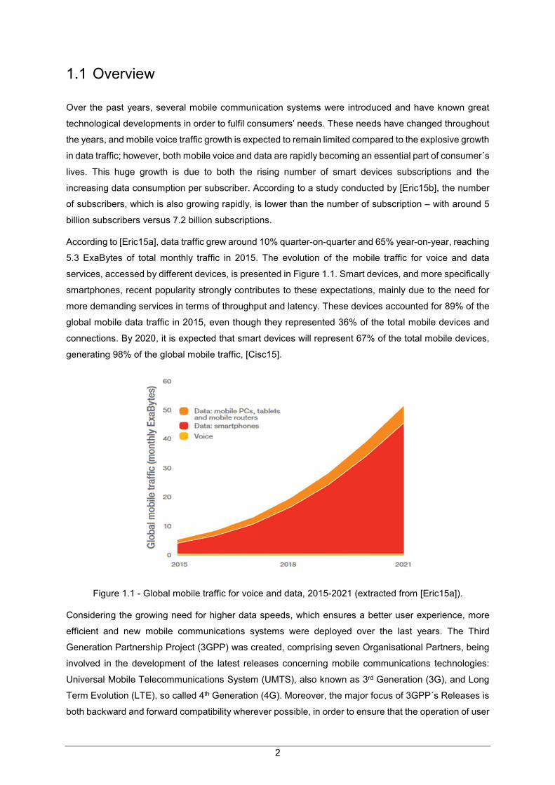
According to [Eric15a], data traffic grew around 10% quarter-on-quarter and 65% year-on-year, reaching

5.3 ExaBytes of total monthly traffic in 2015. The evolution of the mobile traffic for voice and data

services, accessed by different devices, is presented in Figure 1.1. Smart devices, and more specifically

smartphones, recent popularity strongly contributes to these expectations, mainly due to the need for

more demanding services in terms of throughput and latency. These devices accounted for 89% of the

global mobile data traffic in 2015, even though they represented 36% of the total mobile devices and

connections. By 2020, it is expected that smart devices will represent 67% of the total mobile devices,

generating 98% of the global mobile traffic, [Cisc15].

Figure 1.1 - Global mobile traffic for voice and data, 2015-2021 (extracted from [Eric15a]).

Considering the growing need for higher data speeds, which ensures a better user experience, more

efficient and new mobile communications systems were deployed over the last years. The Third

Generation Partnership Project (3GPP) was created, comprising seven Organisational Partners, being

involved in the development of the latest releases concerning mobile communications technologies:

Universal Mobile Telecommunications System (UMTS), also known as 3rd Generation (3G), and Long

Term Evolution (LTE), so called 4th Generation (4G). Moreover, the major focus of 3GPP´s Releases is

both backward and forward compatibility wherever possible, in order to ensure that the operation of user

3

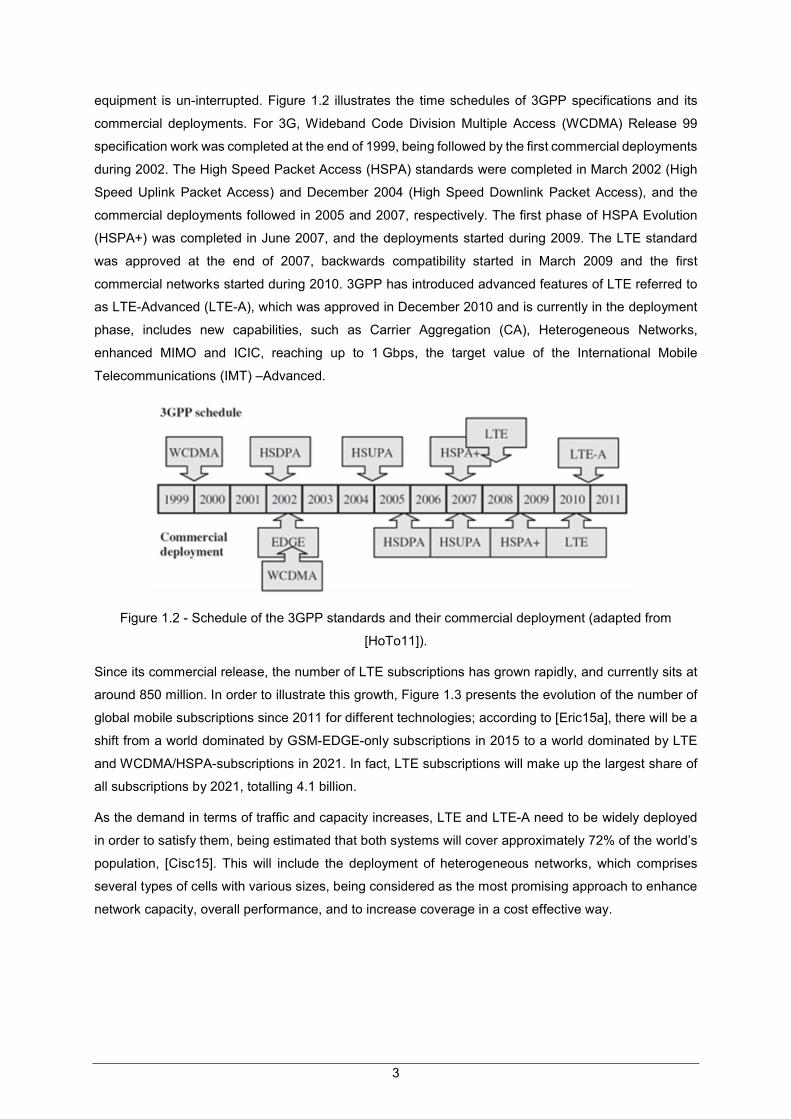
equipment is un-interrupted. Figure 1.2 illustrates the time schedules of 3GPP specifications and its

commercial deployments. For 3G, Wideband Code Division Multiple Access (WCDMA) Release 99

specification work was completed at the end of 1999, being followed by the first commercial deployments

during 2002. The High Speed Packet Access (HSPA) standards were completed in March 2002 (High

Speed Uplink Packet Access) and December 2004 (High Speed Downlink Packet Access), and the

commercial deployments followed in 2005 and 2007, respectively. The first phase of HSPA Evolution

(HSPA+) was completed in June 2007, and the deployments started during 2009. The LTE standard

was approved at the end of 2007, backwards compatibility started in March 2009 and the first

commercial networks started during 2010. 3GPP has introduced advanced features of LTE referred to

as LTE-Advanced (LTE-A), which was approved in December 2010 and is currently in the deployment

phase, includes new capabilities, such as Carrier Aggregation (CA), Heterogeneous Networks,

enhanced MIMO and ICIC, reaching up to 1 Gbps, the target value of the International Mobile

Telecommunications (IMT) –Advanced.

Figure 1.2 - Schedule of the 3GPP standards and their commercial deployment (adapted from

[HoTo11]).

Since its commercial release, the number of LTE subscriptions has grown rapidly, and currently sits at

around 850 million. In order to illustrate this growth, Figure 1.3 presents the evolution of the number of

global mobile subscriptions since 2011 for different technologies; according to [Eric15a], there will be a

shift from a world dominated by GSM-EDGE-only subscriptions in 2015 to a world dominated by LTE

and WCDMA/HSPA-subscriptions in 2021. In fact, LTE subscriptions will make up the largest share of

all subscriptions by 2021, totalling 4.1 billion.

As the demand in terms of traffic and capacity increases, LTE and LTE-A need to be widely deployed

in order to satisfy them, being estimated that both systems will cover approximately 72% of the world’s

population, [Cisc15]. This will include the deployment of heterogeneous networks, which comprises

several types of cells with various sizes, being considered as the most promising approach to enhance

network capacity, overall performance, and to increase coverage in a cost effective way.

4

Figure 1.3 - Area chart with the number of global mobile subscriptions for different technologies, 2011-

2021 (extracted from [Eric15a]).

1.2 Motivation and Contents

The growth in mobile data traffic is due to both the rising number of smartphones subscriptions, in

particular LTE smartphones, and the increasing data consumption per subscriber. The vast cost of

keeping with demand for mobile data is intensifying the pressure on mobile operators’ CAPEX budgets

and accelerating their moves to improve their infrastructure cost base. However, the increase in network

costs and in the total data traffic will be quite a limitation for mobile operators in the future. The need to

reduce networks costs is also driving operators to out-source their whole Radio Access Networks

(RANs), and to seek new mechanisms to acquire and manage sites – frequency and channel bandwidth

selection strategy, type of technology, service coverage design and architecture structure. The purpose

of dimensioning is to estimate the required number of radio base stations needed to support a specified

traffic load in an area, [Syed09]. This number has a fundamental role in cost planning, giving an idea of

the economic impacts in the countries under study.

The main scope of this thesis is to study and describe the nominal RAN planning in LTE, and to compute

the number of cells needed to cover a given area with all the input parameters that the dimensioning

process requires, for different scenarios. Network planning is not a new concept, and has already been

addressed and studied for previous technologies, such as 3G. However, the methods, and some

considerations implemented, are different, as well as the implementation in different scenarios, generally

taking interesting case studies into account, as the Lisbon region with different terrain morphologies and

user densities. Methods and models for coverage and capacity planning are listed and explained in

detail, studying mainly the effects of the number of users in the network, different bandwidths, frequency

band, service throughputs and traffic profiles on a LTE network scenario with multiple-input multiple-

output (MIMO) 2x2.

The traffic distribution depends on the network deployment, country geography and number of active

5

users. Taking the different traffic profiles used in this work into account, it is possible to determine if cells

are limited by coverage or capacity, and due to the use of the frequency domain, load is defined as a

percentage of used Resource Blocks (RBs) over the total available in the system. If the network is

overloaded, the cell is limited by capacity. However, it is important to notice that the load is not directly

proportional to the number of users, because they may require different services and experience

different channel conditions, [Guit16]. Traffic is not equally distributed over a 24-hour period. The busy

hour in data networks is typically in the evening, but data traffic is also generated during the night,

[Noki14]. As such, dimensioning involves planning for peak-hour or busy-hour traffic, i.e., the hour in the

day during which traffic intensity is at its peak. For that reason, only the busy hour is taken into account

in this study.

This thesis was developed in collaboration with Celfinet Portugal, an important global

telecommunications consulting firm. The main output of this thesis is a dimensioning tool that

implements the proposed models, simulates and computes the number of base stations for different

possible scenarios considering different configuration parameters. By varying different input parameters,

the focus is on understanding the impact of these variations on the number of base stations and,

consequently, the cost effectiveness of the network.

In terms of contents, this thesis is divided into five chapters, followed by a set of annexes that serves as

a complement of the developed work. The present chapter makes a brief overview of mobile

communications history evolution, showing the motivation behind the thesis.

In Chapter 2, some fundamental aspects regarding this work are introduced. It provides a brief

description of LTE´s network architecture and radio interface, presenting its main elements. The

description of the services and applications requirements and priorities, followed by the coverage and

capacity considerations. This chapter also presents information about heterogeneous networks, mainly

focusing on the challenges of interference management. To conclude this chapter, one presents some

of the previously developed works related to interference management methods and dimensioning

models, taking cost planning into account.

A full description of the models used in this thesis is provided in Chapter 3, starting by explaining the

various considerations that are of relevance for the development of the present work, such as, coverage,

capacity and throughput calculations, and the relationship in between them. The description of the

implemented simulator is also presented in this chapter, where an illustration shows the simulator

workflow followed by a textual description to facilitate the understanding of the different elements that

compose it. In the end, a brief assessment of the presented models, ensuring that the obtained results

are indeed relevant for this study.

Chapter 4 presents the scenarios description along with the models outputs and their respective

analysis. It begins with a description of the reference scenario, containing all the parameters used in the

simulator. Then, follows the analysis of the results that enables the study of the different parameters

that are of interest, such as cell radius, number of active users and number of cells. Afterwards, relevant

results and figures obtained from the measurements performed in the city of Lisbon and its surrounding

areas are presented.

6

Chapter 5 contains the main conclusions of this thesis, an analysis of the overall obtained results

followed by suggestions for future work.

Some auxiliary information to this thesis is provided in annexes. Annex A presents the expressions that

relate the signal-to-noise-ratio with the throughput per resource block. Path loss was computed using

the COST-231 Walfisch-Ikegami and Okumura-Hata model, detailed in Annex B. Finally, Annex C

presents all the municipalities and its districts under study in this thesis, taking into account the area and

number of inhabitants of each district, as well as the reference user density used in the simulations.

7

Chapter 2

Fundamental Concepts and

State of the Art

2 Fundamental

Concepts and

State of the Art

This chapter provides an overview of LTE and LTE-A systems, mainly focussing on coverage and

capacity dimensioning. The overall network architecture is presented in Section 2.1, the main technical

features of the radio interface is presented in Section 2.2. The services and applications are analysed

in Section 2.3, while the study of coverage and capacity planning, and also heterogeneous networks

aspects that are more relevant for this thesis, are presented in Section 2.4 and 2.5, respectively. Finally,

the state of the art concerning the scope of this thesis is presented in Section 2.6.

8

2.1 Network Architecture

In this section information on LTE and LTE-A architecture is introduced, based on [3GPP16], [Alca09],

[HoTo11].

LTE and LTE-A were designed with the purpose of developing a radio access technology in which

services are packet-switched rather than being circuit-switched, the latter being the model in earlier

systems. Additionally, the standards evolution of mobile communications has been accompanied by an

evolution of the complete system resulting in the System Architecture Evolution (SAE), which includes

the Evolved-Packet-Core (EPC)-network. The Evolved-Packet System (EPS) is constituted by the LTE

radio and SAE, and both the radio and network-core access are packet-switched.

The evolution of the LTE architecture is characterised by progressively lower latencies, reduced costs

and optimised network performances. To achieve these requirements, as well as reducing the

complexity experienced in previous network architectures, LTE was designed to contain fewer network

nodes.

Figure 2.1 shows the system architecture for EPS, which provides all IP based connectivity. As Figure

2.1 shows, the architecture is divided into four main sections: User Equipment (UE), E-UTRAN, EPC

and Services Domain.

Figure 2.1. System Architecture for E-UTRAN only Network (extracted from [HoTo11]).

9

At the highest level, two main components should be addressed: the core Network (EPC) and the

Access-Network (E-UTRAN). While the core network consists of some logical nodes, the access

network is built around one node called the Evolved Node B (eNB), which connects to the UEs.

The eNBs are typically interconnected via the interface, known as X2, and the connection between this

network element and EPC is achieved through the S1 interface. For normal user traffic, as opposed to

broadcasting, there is no centralised controller E-UTRAN, therefore the E-UTRAN architecture is said

to be flat.

LTE´s RAN is also responsible for all radio related functions, including Radio Resource Management,

which covers functions related to the Control Plane, Header Compression helping to ensure an efficient

use of radio interface by compressing the IP Packets headers, and Security where all data sent over the

radio interface is encrypted. These functions are responsible for improving radio interface performance,

which is further discussed in what follows.

The EPC is responsible for the overall control of the UE and establishment of bearers. The main logical

nodes of the EPC are Packet Data Network (PDN) Gateway, Serving Gateway (S-GW) and Mobility

Management Entity (MME). All logical nodes and their functions are discussed in further detail below:

Home Subscriber Server (HSS): A central database that contains users SAE subscription data

and also provides support functions in access authorisation, user authentication, call and

session setup and mobility management.

Policy Control and Charging Rules Function (PCRF): It is responsible for efficient policy and

charging control. The PCRF function is part of the larger Policy Charging Control (PCC)

architecture, which also includes Policy and Charging Enforcement Function (PCEF), located

in the P-GW. Combined, the elements of the PCC provide quality-of-service (QoS) control.

Packet Data Network Gateway (P-GW): Provides connectivity between UE and external IP

packet data networks. It is responsible for IP address allocation for the UE and covers functions

like charging support, policy enforcement and lawful interception of user traffic.

Serving Gateway (S-GW): The transfer of all user IP traffic is ensured by this node, which

connects E-UTRAN and EPC. It acts as the anchor for mobility between LTE and other 3GPP

technologies (such as UMTS) and as the mobility anchor for the user plane.

Mobility Management Entity (MME): It is considered the main control node for the LTE access

network. It processes the signalling between the UE and the EPC. The MME functions covers

security, mobility management, authentication and retrieval of subscription information from the

HSS.

2.2 Radio Interface

This section presents an overview of the radio interface for LTE and LTE-A, based on [3GPP13],

[3GPP15b], [Bryd13], [HoTo11].

10

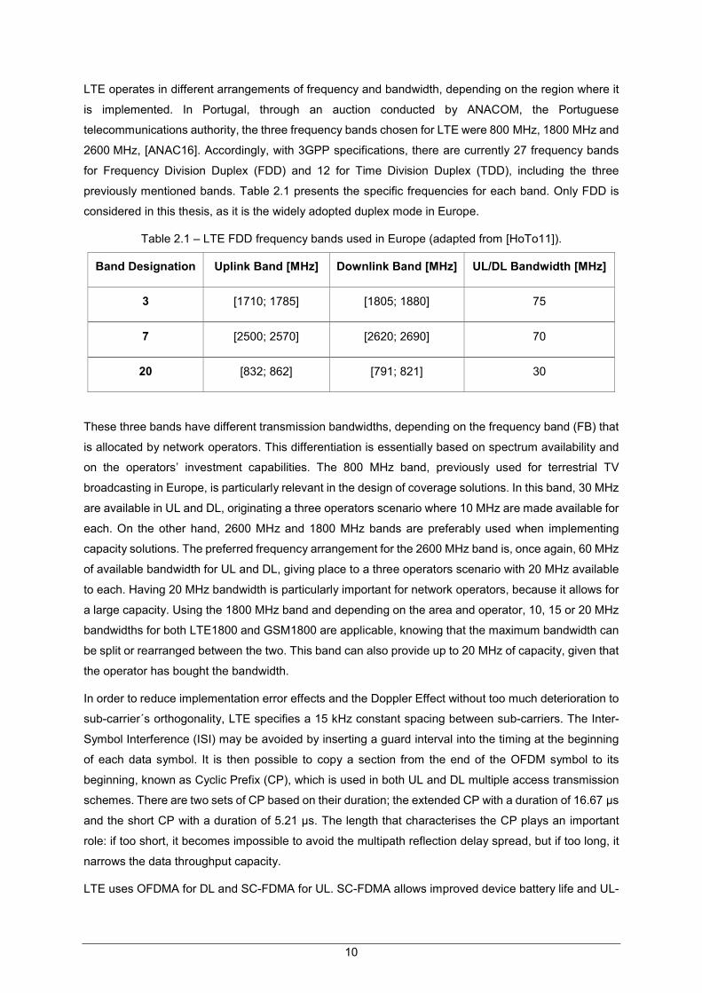
LTE operates in different arrangements of frequency and bandwidth, depending on the region where it

is implemented. In Portugal, through an auction conducted by ANACOM, the Portuguese

telecommunications authority, the three frequency bands chosen for LTE were 800 MHz, 1800 MHz and

2600 MHz, [ANAC16]. Accordingly, with 3GPP specifications, there are currently 27 frequency bands

for Frequency Division Duplex (FDD) and 12 for Time Division Duplex (TDD), including the three

previously mentioned bands. Table 2.1 presents the specific frequencies for each band. Only FDD is

considered in this thesis, as it is the widely adopted duplex mode in Europe.

Table 2.1 – LTE FDD frequency bands used in Europe (adapted from [HoTo11]).

Band Designation Uplink Band [MHz] Downlink Band [MHz] UL/DL Bandwidth [MHz]

3 [1710; 1785] [1805; 1880] 75

7 [2500; 2570] [2620; 2690] 70

20 [832; 862] [791; 821] 30

These three bands have different transmission bandwidths, depending on the frequency band (FB) that

is allocated by network operators. This differentiation is essentially based on spectrum availability and

on the operators’ investment capabilities. The 800 MHz band, previously used for terrestrial TV

broadcasting in Europe, is particularly relevant in the design of coverage solutions. In this band, 30 MHz

are available in UL and DL, originating a three operators scenario where 10 MHz are made available for

each. On the other hand, 2600 MHz and 1800 MHz bands are preferably used when implementing

capacity solutions. The preferred frequency arrangement for the 2600 MHz band is, once again, 60 MHz

of available bandwidth for UL and DL, giving place to a three operators scenario with 20 MHz available

to each. Having 20 MHz bandwidth is particularly important for network operators, because it allows for

a large capacity. Using the 1800 MHz band and depending on the area and operator, 10, 15 or 20 MHz

bandwidths for both LTE1800 and GSM1800 are applicable, knowing that the maximum bandwidth can

be split or rearranged between the two. This band can also provide up to 20 MHz of capacity, given that

the operator has bought the bandwidth.

In order to reduce implementation error effects and the Doppler Effect without too much deterioration to

sub-carrier´s orthogonality, LTE specifies a 15 kHz constant spacing between sub-carriers. The Inter-

Symbol Interference (ISI) may be avoided by inserting a guard interval into the timing at the beginning

of each data symbol. It is then possible to copy a section from the end of the OFDM symbol to its

beginning, known as Cyclic Prefix (CP), which is used in both UL and DL multiple access transmission

schemes. There are two sets of CP based on their duration; the extended CP with a duration of 16.67 µs

and the short CP with a duration of 5.21 µs. The length that characterises the CP plays an important

role: if too short, it becomes impossible to avoid the multipath reflection delay spread, but if too long, it

narrows the data throughput capacity.

LTE uses OFDMA for DL and SC-FDMA for UL. SC-FDMA allows improved device battery life and UL-

11

range, which justifies the different access techniques for UL and DL. The problem associated with

OFDMA in the UL is its high peak to average power ratio (PAPR), which requires high linearity in the

transmitter; because of this, the operating point of the power amplifiers in the transmitter needs to be

lowered off, which in turn lowers the amplifier efficiency, hence the logical use of SC-FDMA in UL,

providing a better power amplifier efficiency. Despite the challenges OFDMA poses to UL, this

modulation scheme benefits over other transmission schemes, having better performance in frequency

selective fading channels, lower complexity of base-band receiver, good spectral properties, handling

multiple bandwidths, link adaption, frequency domain scheduling and compatibility with advanced MIMO

technologies.

LTE uses QPSK, 16-QAM and 64-QAM modulation schemes: 64-QAM carries 6 bits per symbol,

whereas QPSK and 16-QAM carry 2 and 4 bits per symbol, respectively. These last two schemes are

available in all devices, while support for 64-QAM in UL is a UE capability. Adaptive Modulation and

Coding (AMC) was proposed for LTE, as well as to many other 3GPP systems, essentially in order to

improve system capacity and also coverage reliability. By matching coding rates and modulation

schemes to the channel conditions, this system makes possible the efficient and better use of channel

capacities. For any given modulation scheme, the appropriate code rate can be chosen, depending on

channel quality. In order to maximise system throughput and to achieve the maximum channel quality,

higher order modulation schemes and higher code rates can be selected.

For each of the types of duplexing, there is an associated type of frame structure. While Frame Structure

1 is used in FDD, Frame structure 2 is used in TDD. As show in Figure 2.2, LTE radio frames are 10 ms

in duration, these are divided into 10 sub-frames, each sub-frame being 1.0 ms long. Each sub-frame is

further divided into two slots, each with a duration of 0.5 ms. One sub-frame is also the Transmission

Time Interval (TTI). Systems tend to evolve to shorter TTIs, which helps to achieve the requirements of

low latency.

Figure 2.2 - Frame Structure type 1 with short CP (extracted from [Share16]).

Dynamically allocating resources in the frequency domain is another of LTE’s specifications and DL

physical resources can be seen as a time-frequency grid, as illustrated in Figure 2.3.The basic unit of

this grid is the Resource Element (RE) consisting of one sub-carrier during one OFDM symbol. Resource

12

Elements are grouped into Resource Blocks (RBs), each of which consists of a group of 12 sub-carriers,

using a total bandwidth of 180 MHz, and 7 OFDM symbols, when CP has normal length, or 6 symbols

if the extended CP configuration is used. Thus, each RB can have 84 or 72 REs per slot in the time

domain, depending on the CP length.

Figure 2.3 - OFDMA resource allocation in LTE (extracted from [Corr16]).

LTE specifications define bandwidths ranging from 1.4 MHz to 20 MHz. In LTE-A, one of the most

required feature is carrier aggregation (CA), which is used in order to increase bandwidth and,

consequently, the bitrate. Each aggregated carrier is referred to as Component Carrier (CC). LTE-A

allows the aggregation of up to 5 component carriers, each having a bandwidth from 1.4 MHz to 20 MHz,

thus, achieving a maximum aggregated bandwidth of 100 MHz. CA can be used in both TDD and FDD

to facilitate an efficient use of the fragmented spectrum. In FDD, the number of UL component carriers

is always equal or lower than the number of DL component carriers. Table 2.2 shows the relationship

among available bandwidth, number of sub-carriers and the maximum number of allocated RBs.

Table 2.2 - Relationship among bandwidth, number of sub-carriers and of RBs (adapted from

[Corr16]).

One of the fundamental improvements in LTE is the use of multiple antenna techniques, which were

introduced to achieve enhanced system performance both in capacity and coverage. The most common

technique is Multiple Input Multiple Output (MIMO), which enables radio systems to achieve significant

performance gains by using multiple antennas at their transmitters and receivers.

The use of MIMO adds advantages to systems, including greater spectral efficiency, more robust

operations in poor signal conditions and increased data rates for users. MIMO is considered important

Bandwidth [MHz] 1.4 3 5 10 15 20

Number of sub-carriers 72 180 300 600 900 1200

Maximum number of RBs 6 15 25 50 75 100

13

in urban environments, where multipath propagation is significant. In open areas, such as rural locations,

where there is a strong line of sight between the transmitter and receiver, MIMO is less useful.

MIMO can be sub-divided into three main configurations. Spatial multiplexing is one of the configurations

used, which consists of sending signals from two or more different antennas with different data streams.

Subsequent developments have extended this operation and currently LTE-A supports 8x8 MIMO in DL

and 4x4 UL. Transmit Diversity is a different configuration, where the same signal is sent from different

antennas with the same coding, in order to exploit the gains from independent fading between antennas.

Finally, MIMO also relies on Pre-Coding, which exploits transmit diversity by weighting information

streams, i.e., the transmitter sends the coded information to the receiver in order to estimate radio

channel conditions and maximise the received Signal-to-Noise Ratio (SNR).

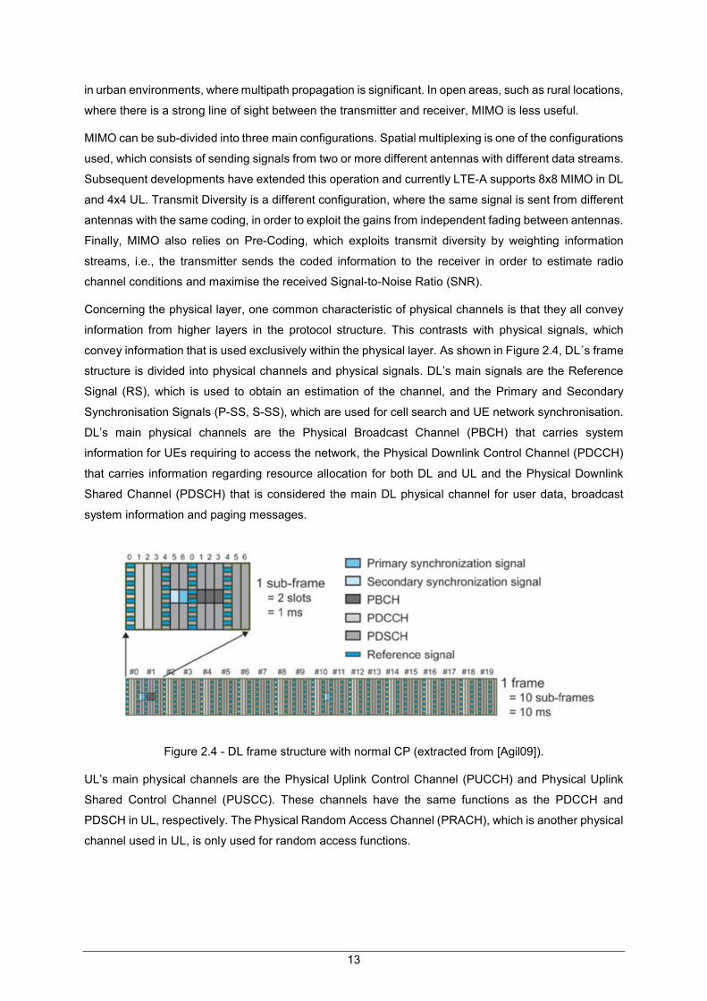
Concerning the physical layer, one common characteristic of physical channels is that they all convey

information from higher layers in the protocol structure. This contrasts with physical signals, which

convey information that is used exclusively within the physical layer. As shown in Figure 2.4, DL´s frame

structure is divided into physical channels and physical signals. DL’s main signals are the Reference

Signal (RS), which is used to obtain an estimation of the channel, and the Primary and Secondary

Synchronisation Signals (P-SS, S-SS), which are used for cell search and UE network synchronisation.

DL’s main physical channels are the Physical Broadcast Channel (PBCH) that carries system

information for UEs requiring to access the network, the Physical Downlink Control Channel (PDCCH)

that carries information regarding resource allocation for both DL and UL and the Physical Downlink

Shared Channel (PDSCH) that is considered the main DL physical channel for user data, broadcast

system information and paging messages.

Figure 2.4 - DL frame structure with normal CP (extracted from [Agil09]).

UL’s main physical channels are the Physical Uplink Control Channel (PUCCH) and Physical Uplink

Shared Control Channel (PUSCC). These channels have the same functions as the PDCCH and

PDSCH in UL, respectively. The Physical Random Access Channel (PRACH), which is another physical

channel used in UL, is only used for random access functions.

14

2.3 Coverage and Capacity

The information in this section regards coverage and capacity planning in LTE-A networks based on

[Syed09], [SeTB11], [Aldh13].

Coverage estimation and capacity evaluation are carried out in Radio Network Dimensioning, which

main objectives are to determine the areas that need to be covered and to calculate the number of base

station sites required to cover the target areas, while fulfilling the capacity and coverage requirements.

In order to fulfil these goals, Network Dimensioning relies on some fundamental parameters, such as

allocated bandwidth, subscriber population, frequency band, geographical area to be covered and traffic

distribution. Radio Link Budget (RLB) is at the heart of coverage planning, where the calculation of the

maximum path loss is based on the required SINR level at the receiver, taking the extent of the

interference caused by traffic into account. The maximum path loss and the minimum received signal in

both UL and DL is converted into the cell radius. This is done using an appropriate propagation model,

which, if required, can be edited to fit the specifications of the deployment area. For a given throughput,

cell edge is defined according to the required SINR, one of the main performance indicators in LTE.

However, if the minimum guaranteed bit rate and subscriber density are given, then it is the cell size

that should be determined.

On the other hand, capacity planning also estimates resources needed to support a specific traffic with

a certain level of QoS (such as throughput). Capacity planning is evaluated by the number of UEs that

can be served by the eNB with a desired quality of service. A UE is considered to be served if it is

receiving RBs from the eNB, and those RBs are able to provide a minimum throughput, depending on

the type of service the UE is using. Having guaranteed a minimum throughput, and knowing the cell

size, it is possible to know the maximum number of users in the network; in this process, the available

spectrum and bandwidth configuration used by the system are particularly important parameters.

For a given estimation of capacity and coverage, the number of RBs available for each user is, [Dout15]:

��/� = ��

��

� (2.1)

where:

�� is the total number of users in the system.

�� is the total number of resource blocks.

The physical layer bit rate for each user, ��/� , can be calculated as follows:

��/�[�� ]=��/�� ·��/� ·��/�� ·log�(�)·��

��[��]

(2.2)

where:

��/�� is the number of sub-carriers per RB (12 for a 15 kHz sub-carrier spacing);

��/�� is the number of symbols per sub-carrier (depending on the CP length);

M is the modulation´s order;

15

�� is the order of the MIMO configuration;

�� is the time transmission interval (1 ms).

Thus, with (2.1) and (2.2) an estimation of the network capacity can be calculated:

�� = ��/�� ·�� ·��/�� ·log�(�)·��

��/�[�� ]·��[��]

� (2.3)

The coverage area radius of a cell is estimated as follows:

��[�� ]= 10

��[�� ] � ��[�� ]� ��[�� ] � ��[��] � ��,��[�� ] � ��[�� ]

�� (2.4)

where:

�� is the transmitted power;

�� and �� are the gain of the transmitting and receiving antennas, respectively;

�� is the minimum receiving power required by the UE;

��,�� is the reference path loss;

�� refers to the margins;

�� is the average power decay.

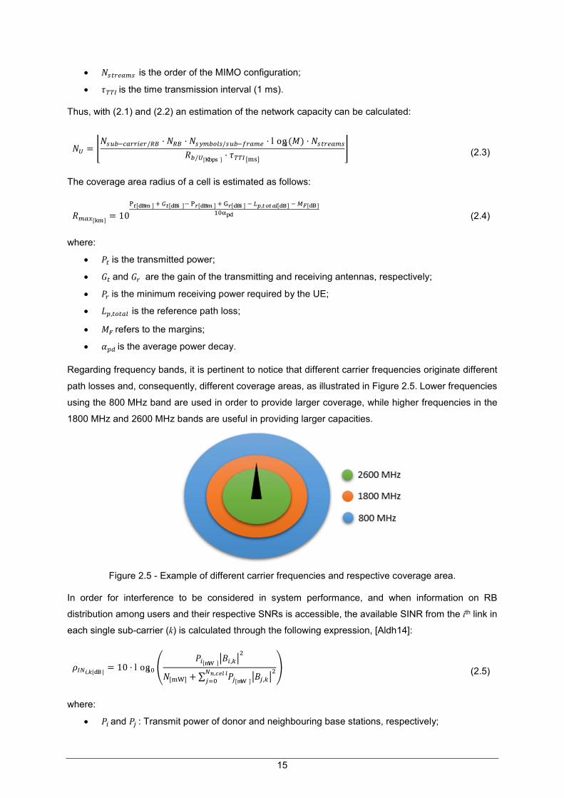
Regarding frequency bands, it is pertinent to notice that different carrier frequencies originate different

path losses and, consequently, different coverage areas, as illustrated in Figure 2.5. Lower frequencies

using the 800 MHz band are used in order to provide larger coverage, while higher frequencies in the

1800 MHz and 2600 MHz bands are useful in providing larger capacities.

Figure 2.5 - Example of different carrier frequencies and respective coverage area.

In order for interference to be considered in system performance, and when information on RB

distribution among users and their respective SNRs is accessible, the available SINR from the ith link in

each single sub-carrier (k) is calculated through the following expression, [Aldh14]:

��,�[�� ] = 10 ·log�� [�� ]

��,��

�[�� ]+ ∑ ��[�� ]��,��

��,��

� (2.5)

where:

�� and �� : Transmit power of donor and neighbouring base stations, respectively;

16

��,� and ��,�: Fading channel gain for donor and neighbouring cell, respectively;

�: Noise power;

��,��: Number of neighbouring cells.

In a severely interference limited scenario, the noise power can be ignored to simplify the calculations

and the above expression can be written as:

��,�[�� ] = 10 ·log�� [�� ]

��,�[�]��

∑ ��[�� ]��,�[�]

��,��

� (2.6)

where B being a function of path loss leads to |�|� = �� , with L being a constant, L= �� depending

on the infrastructure of sender and receiver, α is the path loss exponent, ��,� and ��,� are the distances

from user to donor base station and neighbouring cells respectively as shown Figure 2.6. In addition,

the transmit powers �� and �� are calculated using the expressions in Annex A.

Figure 2.6 - Example of interference scenario in LTE-A Network (extracted from [Aldh13]).

Interference can lead to a severe degradation of SINR and spectrum efficiency, which decreases the

overall capacity of the network, and the expected user’s throughput will not be achieved, especially

regarding cell-edge users. Only the interfering signals that have a power equal or greater than the noise

power are considered, since only these may negatively impact system performance. The increase in

interference and noise generated by the increasing number in users decreases cell coverage, forcing

the cell radius to be smaller and having lower data rates. So, higher data rates are achieved when the

available SINR is high. This performance indicator also depends on MCS, being known that lower order

modulations, e.g., QPSK, are more robust and can better tolerate higher levels of interference, but lower

transmission bit rates are achieved, and for this reason high order modulations are also considered,

such as 16-QAM and 64-QAM, which offer better bit rates, although they are more susceptible to errors

17

due to their sensitivity to noise, interference and channel estimation errors.

If the SINR is sufficiently high, a high-order modulation is more useful and usually preferred. The code

rate can be chosen depending on channel conditions, a higher code rate being used when the SINR is

high, while a lower code rate is used in poor channel conditions. As shown in Figure 2.7, data rates

decrease strongly with the reduction of the SINR, which leads to a reduction of channel capacity. This

problem is particularly relevant in indoor scenarios, because of the extra attenuation associated with

building penetration, which leads to a significant decline of SINR.

Figure 2.7- Throughput per RB in DL vs. SINR for different MCS (extracted from [Pire15]).

Table 2.3 and Table 2.4 show the peak data rates for UL and DL, respectively: UL ones are usually

lower than DL’s due to the limitation of the UE. These peak data rates are calculated by considering the

normal CP usage and the correspondence between bandwidth and available number of RBs for data,

as illustrated in Table 2.2. The bit-rate increases with the bandwidth, the number of RBs, the order of

the coding scheme and ratio, and the order of MIMO.

UL Peak Data Rates [Mbps]

Bandwidth [MHz]

MCS Bits/Symbol 1.4 3.0 5.0 10 15 20

QPSK ½ 1.0 1.0 2.5 4.2 8.4 12.6 16.8

16QAM ½ 2.0 2.0 5.0 8.4 16.8 25.2 33.6

16QAM ¾ 3.0 3.0 7.6 12.6 25.2 37.8 50.4

16 QAM 1/1 4.0 4.0 10.1 16.8 33.6 50.4 67.2

64QAM ¾ 4.5 4.5 11.3 18.9 37.8 56.7 75.6

64QAM 1/1 6.0 6.0 15.1 25.2 50.4 75.6 100.8

Table 2.3 – UL peak data rates not considering MIMO (extracted from [Alme13]).

18

2.4 Services and Applications

The information in this section regards services and applications based on [3GPP15a], [Corr16],

[HoTo11].

Demand for new services and applications is on the rise. Therefore, these days, users face a huge

variety of services and applications with different requirements and purposes. However, the most

popular and also oldest service is voice. With the emergence of data services, voice popularity has been

declining, but it still remains one of the most important services for operators This service is very

predictable, with a constant bit rate, allowing operators to ensure its performance without much effort.

The concern from operators is delay, as it is the main responsible for the phone call overall quality. On

the other hand, data services require more attention from operators, since these services are very

demanding in terms of bitrate, delay and duration, but also because they generate huge data traffic.

Data services, such as video streaming and web browsing, require more traffic capacity than ever, and

pose greater challenges to operators. In order to face these challenges, and especially to provide QoS

guarantees, 3GPP proposed four different QoS classes related to the desired type of service and quality:

Conversational Services comprises voice and real-time multimedia messaging, such as VoIP

and Video Conferencing. In real time conversations, it is fundamental to preserve time relation

DL Peak Data Rates [Mbps]

Bandwidth [MHz]

MCS Bits/Symbol MIMO usage 1.4 3.0 5.0 10 15 20

QPSK ½ 1.0 - 1.0 2.5 4.2 8.4 12.6 16.8

16 QAM ½ 2.0 - 2.0 5.0 8.4 16.8 25.2 33.6

16 QAM ¾ 3.0 - 3.0 7.6 12.6 25.2 37.8 50.4

64 QAM ¾ 4.5 - 4.5 11.3 18.9 37.8 56.7 75.6

64 QAM 1/1 6.0 - 6.0 15.1 25.2 50.4 75.6 100.8

64 QAM ¾ 9.0 2 x 2 MIMO 9.1 22.7 37.8 75.6 113.4 151.2

64 QAM 1/1 12.0 2 x 2 MIMO 12.1 30.2 50.4 100.8 151.2 201.6

64 QAM 1/1 24.0 4 x 4 MIMO 24.2 60.5 100.8 201.6 302.4 403.2

Table 2.4 - DL peak data rates (extracted from [Alme13]).

19

(variation) between information entities in the stream and guarantee low transfer delays. This is

the most delay sensitive service class.

Streaming Services are still dependent on the time relation between both ends of the stream,

but delay requirements are not as strict as in Conversational, since these services have

unidirectional data flows. Video on demand is an example of this class.

Interactive Services include web browsing, automatic data base enquiries and server access.

This class is applied when one end-user requests data from remote equipment, e.g., a server,

and is characterised by requesting a response pattern from the end-user and preserving the

payload contents.

Background Services, where one end-user sends and receives data-files in the background, are

mainly characterised by the fact that the destination is not expecting the data within a certain

time frame and it can be stored to be read later on, thus being less delivery-time sensitive, e.g.,

e-mail, SMS, databases download and reception of measurement records.

Table 2.5 presents the QoS classes mentioned above, namely real time requirements, data flows,

symmetry, guaranteed bit rate necessity, time delay, restrictions, extended use of data buffers and traffic

burstiness. Included among the specifications are the limited set of signalled QoS parameters, which

were then optimised for SAE:

QoS Class identifier (QCI) is an index that identifies a set of values for priority, delay and loss

rate. QCI is signalled instead of separately signalling the values of these parameters. Operators

can create additional classes within their network.

Allocation and Retention Priority (ARP) indicates the priority of the bearer compared to other

bearers, providing the basis for admission control in bearer set-up and in congestion situations

if bearers need to be dropped.

Maximum Bit Rate (MBR) identifies the maximum bit rate for the bearer.

Guaranteed Bit Rate (GBR) identifies the guaranteed bit rate to the bearer.

Aggregated Maximum Bit Rate (AMBR) indicates the total maximum bit rate a UE may have for

all bearers in the same PDN connection.

Service Class Conversational Streaming Interactive Background

Real Time ✓ ✓ × ×

Symmetric ✓ × × ×

Bit Rate Guaranteed Guaranteed Non-Guaranteed Non-Guaranteed

Delay Minimum fixed Minimum variable Moderate Variable High variable

Buffer × ✓ ✓ ✓

Bursty × × ✓ ✓

Example Voice/Video Call Video Streaming Web Browsing SMS, E-mail

Table 2.5 - QoS service classes summary, according to 3GPP (adapted from [3GPP15a]).

20

Table 2.6 shows the nine QoS Class Identifiers and the associated set of QoS characteristics, as defined

in 3GPP standards. Resource Type indicates which classes are categorised as GBR and which are

categorised as non-GBR, Priority defines the priority for the packet scheduling and higher-priority

packets. A rating of 1 corresponds to the highest priority. Delay Budget helps the packet scheduler to

maintain the delay requirements for the bearers, and Loss Rate defines the percentage of higher layer

packets, e.g., IP packets, that are lost when the network is not congested, and also helps to use

appropriate Radio Link Control (RLC) settings.

Table 2.6 - QoS parameters for QCI (extracted from [SeTB11]).

QCI Resource

Type Priority

Packet Delay

Budget [ms]

Packet Error

Loss Rate Example Services

1

GBR

2 100 10-2 Conversational Voice

2 4 150 10-3 Conversational Video (Live

Streaming)

3 5 300 10-6 Non-Conversational Video

(Buffered Streaming)

4 3 50 10-3 Real Time Gaming

5

Non-GBR

1 100 10-6 IMS Signalling

6 7 100 10-3 Voice, Video (Live Streaming),

Interactive Gaming

7 6 300 10-6 Video (Buffered Streaming)

8 8

300 10-6

TCP-based (e.g. www, e-mail,

chat, FTP, p2p file sharing,

progressive video, etc.) 9 9

In the event of capacity shortage, given the increasing number of mobile broadband data users and

bandwidth intensive services, the QoS for end users may be degraded. All these services have data

rate requirements that vary depending on their purpose. While voice services require lower data rates

with only tens of kbps, web browsing, file transfer and streaming require higher bit rate transmissions

going up to several tens of Mbps. Conversational and Streaming services can be used for applications

that have an associated GBR, e.g., voice usually requires 8 to 64 kbps and music streaming 128 to

320 kbps constant data rate over the network, [AnJa15], these values for guaranteed bit-rate services

being highlighted in bold in Table 2.7. On the other hand, Interactive and Background services, such as

web browsing and FTP applications, do not guaranteed any particular bit-rate, as the nature of these

applications requires them to fluctuate according to user’s requirements.

The service’s minimum and maximum throughputs are presented in Table 2.7, with their respective

service class. The maximum values try to guarantee a high QoS, and while these can be raised even

21

further in most cases, like streaming and browsing, guaranteeing an even higher QoS, VoIP is capped

by the value shown. The considered minimum throughputs are the ones that guarantee a minimum QoS.

Table 2.7 - Services characteristics.

Service Service Class Minimum

Throughput [Mbps]

Maximum

Throughput [Mbps]

VoIP Conversational 0.032 0.064

Chat Background 0.064 0.384

Streaming Streaming 1 13

Web Browsing Interactive 1 150

FTP Interactive 1 150

Email Background 1 150

P2P Interactive 1 150

2.5 Heterogeneous Networks

This section discusses specific aspects of heterogeneous networks and advanced approaches for

optimised interference management, based on [3GPP16b], [3GPP16c], [YeTa11], [Ali15].

Mobile broadband traffic is growing rapidly, thanks to the increasing popularity of connected devices

and rising data consumption per user. Consumers have come to expect a consistent, high quality and

seamless mobile broadband experience wherever they are. In order to fulfil these demands and

intensifying competition, operators need to improve network performance by expanding capacity and

coverage in a smooth, cost-effective way. One of the most promising low-cost approaches is to deploy

a Heterogeneous Network (HetNet), which involves a mix of radio technologies and cell types working

together to spread traffic loads and also to deliver the additional capacity, coverage and speed needed

to maintain perform and service quality, while reusing spectrum most efficiently. In HetNets, the cells of

different sizes are referred to as macro-, micro-, pico- and femto-cells, listed in order of decreasing

transmission power and implementation cost. Macro-cells provide wide coverage area, up to a few tens

of kilometres, while micro- and pico- can have a coverage range from a few hundred metres to a few

kilometres; femto-cells cover an even smaller area, such as a house or an office, so their coverage

range is up to a few tens of metres. While macro- and micro-cells provide essential coverage, small

ones like pico- and femto-cells can be deployed as hotspots in capacity starved locations, but also to

eliminate coverage holes in a macro-cell network. The relay node approach is another type of low-power

base station added to Release 10 specifications and relay stations serve similar sizes of footprints as

22

pico-cells. To expand an existing macro-cell network, operators need to improve and densify it, adding

more sectors per eNB or deploying more macro-cells eNBs, and add integrated small cells within their

existing network, in strategic locations. With these deployment strategies, high traffic volumes and data

rates can be supported. An overview of a HetNet is illustrated in Figure 2.8.

Figure 2.8 – LTE-A Heterogeneous Network (extracted from [JaMa13]).

One of the main challenges of HetNets is the severe interference between neighbouring small cells and

between small and macro-cells. Generally, there are two types of interference, co-tier or intra-cell

interference. and cross-tier or inter-cell interference; while the former occurs among network elements

that belong to the same tier in the network, the latter occurs among network elements that belong to

different tiers of the network. These types of interference occur when macro- and small cells are

operating simultaneously in the same spectrum.

As a more usual implementation mode, Closed Access mode is generally deployed in private scenarios,

and a group of registered users called Closed Subscriber Group (CSG) has the permission to access

the femto-cell, hence CSG may cause excess interference to the surrounding network when sharing the

same spectrum with other tiers. Thus, it is essential to adopt an effective and robust interference

management and intelligent bandwidth allocation among tiers, in order to enhance the performance of

the multi-tier networks.

Concerning operators that own more than one frequency band, the simplest type of spectrum planning

consists of assigning different operating frequencies to users being served by first tier-devices, like

macro-cells, and to users served by second-tier services, like small ones. Using a dedicated carrier in

small cells avoids interference with macro-cells, and the former can absorb larger amounts of traffic

coming through the macro-cell network, enabling wider coverage areas. Although shared-carrier

deployments offer lower coverage ranges than one with dedicated carriers, it is often an effective

solution for coverage, especially indoors. With shared carriers, small cells use one of the same carriers

assigned to the macro tier, however, these cannot be placed too close to the high-power macro-cell.

When operators have low spectrum-holdings, shared carrier is the only option available for deployment

of small cells. On the other hand, for operators with some available spectrum, each second-tier device

can choose from multiple accessible frequency bands for one at which it will transmit and as a result

interference from same-tier devices is further mitigated. Although most network operators are capacity

constrained due to the limited spectrum, those who can spare the extra spectrum can consider carrier

23

aggregation in order to improve channel utilisation efficiency. When using carrier aggregation, there is

a serving cell for each carrier. The coverage of these cells may differ, since carriers in different frequency

bands experience different path losses, which increase with frequency. One of the serving cells is

designated the Primary Cell (PCell), while the rest are known as Secondary Cells (SCells), Figure 2.9.

Figure 2.9 – LTE-A HetNet Multi-Site Carrier Aggregation (extracted from [Ali15]).

Initially, macro-cells with full coverage area can serve as PCells and small cells as SCells, based on the

centralised architecture, but when considering that requiring a centralised architecture is not in the goal

of LTE-A networks, macro- and small cells may operate with their own control and signalling on both

frequency layers. In this case, both macro- and small cells allocate different frequency layers to their

respective PCells and SCells. Scells may transmit data with lower power to avoid interfering with the

Pcells of the other layer; depending on the implementation of the radio resource management and

scheduling algorithm, UEs close to the base station can be scheduled with low power Scell allocations,

while cell edge ones are allocated to the Pcell. Using CA with cross-carrier scheduling, for full protection

of the control region, it is possible to map the Physical DL control channels (PDCCH) on different carriers

in the large and small cells, hence, reducing the risk of PDCCH interference.

Additionally, one of the major issues in HetNet planning is to ensure that small cells properly serve

enough UEs, which can be guaranteed by extending the coverage area served by the small cells, which

is achieved by the use of a positive cell selection offset to the strongest received DL signal of the small

cell. This extended area is called Cell Range Extension (CRE). However, ICI has become a more severe

problem in the CRE area, which can be mitigated by using Enhanced Inter-Cell Interference

Coordination (eICIC), an advanced ICIC technology introduced in 3GPP Release 10, which has evolved

to better support heterogeneous network deployments, especially interference management for control

and data channels. This advanced technique uses a power and frequency domain, but the major change

compared to ICIC is the addition of a time domain ICIC, made possible through the use of Almost Blank

Sub-frames (ABS). ABS only includes control channels and cell-specific reference signals, user data is

left out, being transmitted with reduced power. When eICIC is used, ABS patterns are configured in

semi-statically and signalled between the macro- and small cells over the X2 interface. ICIC has evolved

in LTE Release 11 to further enhanced ICIC (feICIC), the focus being interference handling by the UE

through ICI cancellation for control signals, enabling even further cell range extension. It is also

important to notice that eCIC and feICIC are especially important when CA is not in use. Another way

to limit ICI, while further exploiting the benefits of distributed multiple antenna systems, is to use

24

Coordinated Multi-Point (CoMP), introduced in LTE-A Release 11. The main reason to introduce CoMP

is to improve network performance, especially at cell edges, where performance may be degraded, the

basic idea being to transform ICI into a useful signal. With CoMP, a number of transmission and

reception points can be dynamically coordinated to provide a service and to ensure that a UE is using

both the best DL and UL carriers in a heterogeneous network.

2.6 State of the Art

This section presents previous work developed by a variety of authors on coverage and capacity

dimensioning, its associated costs, as well as interference management, showcasing their main

conclusions and results obtained through simulations and algorithm analysis.

[HaHe11] investigates the performance of an LTE-A based network in different spectrum bands. The

authors analyse the performance of a single carrier in different bandwidths in two different spectrum

bands, 800 MHz and 2.6 GHz. Simulations show that an increased system bandwidth may not

necessarily result in a higher system throughput, since in some cases a low frequency (i.e., 800 MHz)

system is superior to a high frequency deployment (i.e., 2.6 GHz), although the operating bandwidth of

the former is half of the one of the latter. The authors also verified that the deployment of a CA-based

system increases cell and user throughputs significantly by extending the operating bandwidth.

[AnMa16] presents a comparison between two scenarios of CA, one that combines low and high

spectrum bands (e.g., 800 MHz and 2.6 GHz) and the other combining mid and high spectrum bands

(e.g., 1800 MHz and 2.6 GHz). In both cases, CA provides benefits by improving the peak speeds to

compatible devices within the coverage area of the two bands. However, the combination of bands that

are more closely matched in frequency, such as 1800 MHz with 2.6 GHz, offer a better synergy for

operators from a capacity and coverage perspective.

[NiJa14] introduced a model for evaluation of the total deployment costs of heterogeneous wireless

access networks. The model uses up to date inputs of the unit cost of particular base station classes,

which is characterised with specific coverage and capacity parameters. The authors analysed

deployments in both the 800 MHz and 2.6 GHz bands, as well as the scenario of aggregated carriers in

these bands. They concluded that while the re-use of the existing macro-cell sites with the low-end

frequency carriers at 800 MHz represents moderate cost-efficiency, the solution to deploy the denser

network at 2.6 GHz with re-use of existing sites is more cost-efficient than the solution to construct new

sites with 800 MHz. Hence, the key finding is that the use of CA for moderate demand levels will

significantly increase the cost-effectiveness of the macro-cell cellular deployment. On the other hand,

indoor deployed femto-cells are most cost efficient only for the higher to extreme user demand.

[Garc13] focuses on the development of a strategic network planning tool and a set of optimisation

algorithms to solve the services distribution problem over a set of technologies, and minimise the total

cost of network deployment. The approach is divided into two main parts, a dimensioning and planning

25

module, and a bio-inspired optimisation one. The goal of both modules is to provide a set of algorithms

capable of performing the dimensioning process of a multi-technological RAN, providing information

about the number, type and location of the required base stations in order to satisfy specific coverage

and capacity constraints, and the optimisation of the traffic demand’s distribution over the different

technologies to be deployed. The author has tested the proposed algorithms in a set of different

scenarios. Moreover, a study simulating the deployment of a LTE network with different spectrum

allocation in the 800 MHz, 1800 MHz, and 2600 MHz has been carried out. Improvements, in terms of

investment cost, and thus a reduction on services provision costs, are observed for all simulated cases.

The experiments performed in this work are focused on the Spanish case, but the algorithms can be

easily adopted to carry out similar studies in any other European country.

The authors of [AtZa14] present a partially combinatorial optimisation algorithm positioning of

heterogeneous cells with relay nodes for an LTE network with non-uniform throughput user

requirements. The main goals of this algorithm are to exploit LTE characteristics and to identify an

optimum solution that meets the operator’s requirements in terms of coverage and capacity in a given

area, with the minimum number of base-stations, and hence, cost.

[ShIs13] analysed the efficiency of different deployment locations of femto-cells. Simulations show that

by deploying femto-cells at an appropriate location, femto- to macro-cells interference can be mitigated,

coverage almost reaching the double, while the data rate received by the end user increases by 28%

on average, compared to a random deployment.

[VuKw15] proposed an algorithm aimed to select an appropriate ABS ratio based on the SINR for macro-

to femto-cell networks, in order to reduce the dominant cross-tier interference. Authors also proposed a

coalition algorithm to help small cells collaborate efficiently in order to reduce mutual interference.

Taking various environments into account, simulations show that the small cell performance of their

proposed algorithm is better than that of the existing ABS frameworks with a high rate in terms of user

throughput.

Fractional Frequency Reuse (FFR) is a simple and effective mechanism for interference management

in OFDMA-based HetNets. In [SaHo13], the authors presented a broad comparison among three

traditional FFR schemes and proposed a FFR scheme for two-tier HetNets in LTE-A. This comparison

is performed by using Monte Carlo simulations considering performance metrics such as outage

probability, network throughput, and spectral efficiency. Simulation results show that the average gains

in spectral efficiency (b/s/Hz) of the network are significantly higher for the proposed scheme compared

to the other three FFR schemes.

[Alme13] focuses on evaluation of LTE performance in urban scenarios concerning ICI via antenna

aspects. This analysis addressed the 800 MHz, 1800 MHZ and 2600 MHz bands. Most performance

enhancements are achieved when electrical down-tilt variations are considered, followed by the height

of the antennas, the transmitter output power and mechanical down-tilt. The author also concluded that

for the low load scenario, the 800 MHz band suffers the highest interference impact. For the high load

scenario, simulations results show that the ICI impact on throughput increases with the frequency band

while the reduction of SNR into SINR decreases.

26

In [Seif12], a detailed LTE radio network dimensioning procedure, including frequency, coverage and

capacity analysis, has been performed in order to prepare a radio planning guideline considering

possible network implementation in the city of Tripoli (Libya). With this aim in mind, a step-by-step

method followed, starting from gathering planning information, which went up to coverage and capacity

analysis. In terms of coverage, the cell radius and the required number of cells for dense urban, urban

and suburban scenarios were computed, taking the link budget and propagation model calculations into

account. The obtained cell radius, for dense urban scenario, is higher than the one for the other

scenarios. As for capacity, the number of cells was computed for the same environments, considering

three different service packages. In order to satisfy the traffic requirements of both coverage and

capacity, the maximum number of sites obtained from capacity and coverage calculations was chosen.

At the end, the link level of the LTE network is simulated for both UL and DL, in order to get a closer

view of the impact of the SNR on Bit Error Rate (BER) and Block Error Rate (BLER). From the link level,

the authors concluded that, as the BER or BLER increases, the SNR decreases, and vice-versa. It was

also verified that the relation BER vs. SNR or BLER vs. SNR varies depending on many parameters,

such as modulation scheme, code rate, channel type and antenna configuration. For instance, it is

shown that BER and BLER can be improved by increasing the number of receiving antennas, even

though the number of transmitting antennas does not affect them. Another conclusion was that receiver

diversity affects the SNR. With the increase of MIMO order, an increase on SNR was verified.

[IbHa14] indicates the implementation of a dimensioning tool for the LTE planning process that follows

the dimensioning algorithms designed by Ericsson [Eric10]. The model consider the concepts and

calculations associated with coverage and capacity planning that are essential to the dimensioning

process. The tool was developed using C# (C Sharp) programming language and two case studies were

analysed. In the first case, some parameters were varied in relation to the reference scenario, such as

the environment, eNB noise figure and height. The authors concluded that the number of cells increases

due to the increase in noise. In addition, areas with dense urban characteristics need more sites to meet

the required bitrate, and, in rural areas with fewer users, the number of sites was lower compared to the

one obtained for the urban ones. They also verified that the decrease in height results in a smaller

coverage area, which leads to an increase in the number of sites. In the second case, the area and most

of the inputs are different in relation to the reference scenario, but the main parameter studied was the

antenna gain. The authors concluded that the area type and decreased gain were the primarily

responsible elements for the several reduction in the area covered by each site. Though there is a slight

decrease in the noise figure, it does not gravely affect the site's coverage area.

27

Chapter 3

Models and Simulator

Description

3 Models and

Simulator

Description

A description of the models used in this thesis is provided in this chapter, in which their mathematical

formulation and implementation are detailed. At the end of this chapter, a brief assessment of the

presented simulator is done.

28

3.1 Model Development

This section provides a description of the models developed in this thesis, with their mathematical

formulation.

3.1.1 Dimensioning Process

Dimensioning is the initial phase of network planning. It provides the first estimate of the network element

count as well as the capacity of these elements. The purpose of dimensioning is to estimate the required

number of base stations needed to support a specified traffic load in an area [Syed09]. Dimensioning is

a part of the whole planning process, which also includes detailed planning and optimisation of the radio

network. The aim of this whole exercise is to provide a model to design the cellular network such that it

meets the quality requirements set forth by service providers, operators or even the end-users. However,

the difficulty lies on combining all requirements in an optimal way and to design a cost-effective network

[Seif12]. The cellular network dimensioning can be divided into different phases as seen in Figure 3.1.

Dimensioning provides the first, quick assessment of the probable radio network configuration, and this

process varies from place to place, depending on the dominating factor, which can be capacity or

coverage. This is a very important process in network deployment, because it can be modified to fit any

needs of any cellular network.

Figure 3.1 - LTE network dimensioning.

Dimensioning uses relatively simple models and methods that reduce the time required for this process.

On the other hand, a dimensioning tool should be accurate enough to provide results with an acceptable

level of accuracy, when loaded with subscriber base and expected traffic profile, and a proper set of

inputs is vital to yield accurate outputs. LTE planning inputs is the first step in dimensioning, and can

broadly be divided into coverage-, capacity- and quality-related, which are technology dependent

[Seif12]. These inputs as well as outputs are briefly discussed in the following section. The basic

requirements for the cellular network are to meet coverage, capacity and quality targets. These

requirements are also related to how the end user experiences the network. According to, [Seif12], the

29

dimensioning process is generally carried out as follows. In a first approach, the maximum allowable

network load is considered to determine the site density through the link budget, which is called a

coverage limited planning; coverage estimation is used to determine the maximum coverage area of

each base station, but it is not necessary that a suitable connection between the eNB and UE can be

established in the coverage area. Furthermore, coverage planning also includes coverage analysis, one

of the most critical step in the design of an LTE radio network. In the second approach, the user profile

is used to iteratively determine the site density, i.e., the network planner must specify the traffic profile

loading of the network, including data rates and coverage requirements along with the maximum

permissible network load; after computing the cell radius from coverage planning, the number of users

inside the cell is computed, and the traffic profile of each user is considered to determine if the maximum

permissible network load is exceeded. In this case, the planning is limited by capacity. Based on such

criteria, the final target of planning, namely, defining network design and deployment requirements can

be achieved. Last but not least, the outputs of the dimensioning phase are used to estimate the feasibility

and cost of the network, being further used in the detailed network planning, and also for core network

planning. For a clear understanding, each of the steps is thoroughly explained in the coming sections.

3.1.2 Inputs and Outputs of LTE Dimensioning

Radio cellular network dimensioning requires some fundamental elements, like geographical area to be

covered, frequency band, allocated bandwidth, MIMO order, population density and traffic distribution.

This section discusses all the dimensioning inputs used in the development of model. As can be seen

in previous section, dimension inputs can be divided into three categories, i.e., quality-, coverage- and

capacity-related ones.

In this thesis, quality-related inputs include the minimum throughput at the cell edge in DL and UL. These

inputs are used to compute SINR, but are also connected to the investment that the operator wishes to

make, and the quality that it wants to offer to the end-users at the cell edge. In terms of coverage, it is

also important to notice that the considered minimum throughput per RB is obtained by taking the

minimum reference throughput that end-users experience at the cell edge into account, guaranteeing

10% of RBs of the maximum number of RBs of each bandwidth. Basically, the minimum throughput per

RB is obtained by dividing the reference throughput by the ensured number of RBs at the cell edge. In

this case, 10% of the maximum number of RBs associated with each frequency is taken as reference.

Radio Link Budget (RLB) is of central importance to coverage planning, inputs including transmitter

power, transmitter and receiver antenna systems, number and type of antennas, propagation models

and their respective parameters, and conventional system gains and losses. Additionally, channel types

(Pedestrian, Vehicular) and geographical information, such as area information (urban, suburban, rural)

and size of each area type to be covered, are needed to start the coverage dimensioning exercise.

Coverage depends on the area covered by the signal, which also depends on radio propagation

characteristics in the given area, and varies from region to region, hence, it should be studied carefully.

Furthermore, the required outdoor and indoor coverage probabilities play a vital role in the determination

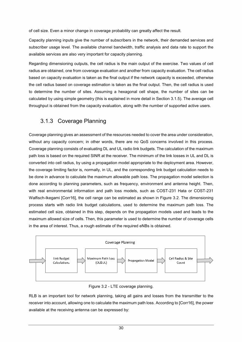
30

of cell size. Even a minor change in coverage probability can greatly affect the result.

Capacity planning inputs give the number of subscribers in the network, their demanded services and

subscriber usage level. The available channel bandwidth, traffic analysis and data rate to support the

available services are also very important for capacity planning.

Regarding dimensioning outputs, the cell radius is the main output of the exercise. Two values of cell

radius are obtained, one from coverage evaluation and another from capacity evaluation. The cell radius

based on capacity evaluation is taken as the final output if the network capacity is exceeded, otherwise

the cell radius based on coverage estimation is taken as the final output. Then, the cell radius is used

to determine the number of sites. Assuming a hexagonal cell shape, the number of sites can be

calculated by using simple geometry (this is explained in more detail in Section 3.1.5). The average cell

throughput is obtained from the capacity evaluation, along with the number of supported active users.

3.1.3 Coverage Planning

Coverage planning gives an assessment of the resources needed to cover the area under consideration,

without any capacity concern; in other words, there are no QoS concerns involved in this process.

Coverage planning consists of evaluating DL and UL radio link budgets. The calculation of the maximum

path loss is based on the required SINR at the receiver. The minimum of the link losses in UL and DL is

converted into cell radius, by using a propagation model appropriate to the deployment area. However,

the coverage limiting factor is, normally, in UL, and the corresponding link budget calculation needs to

be done in advance to calculate the maximum allowable path loss. The propagation model selection is

done according to planning parameters, such as frequency, environment and antenna height. Then,

with real environmental information and path loss models, such as COST-231 Hata or COST-231

Walfisch-Ikegami [Corr16], the cell range can be estimated as shown in Figure 3.2. The dimensioning

process starts with radio link budget calculations, used to determine the maximum path loss. The

estimated cell size, obtained in this step, depends on the propagation models used and leads to the

maximum allowed size of cells. Then, this parameter is used to determine the number of coverage cells

in the area of interest. Thus, a rough estimate of the required eNBs is obtained.

Figure 3.2 - LTE coverage planning.

RLB is an important tool for network planning, taking all gains and losses from the transmitter to the

receiver into account, allowing one to calculate the maximum path loss. According to [Corr16], the power

available at the receiving antenna can be expressed by:

31

��[�� ]= ��[�� ]

+ ��[��] + ��[��] − ��,��[�� ] (3.1)

where:

��: power to fed to the transmitting antenna;

��: gain of the receiving antenna;

��: gain of the transmitting antenna;

��,��: total path loss.

While the BS antenna gain depends essentially on the antenna type and on the number of sectors, the

UE one depends on the type of device. The power fed to the transmitting antenna is defined as:

��[�� ]= ��[�� ]

− ��[�� ] (3.2)

where:

�� : transmitter output power;

��: loss in the cable between the transmitter and the antenna for DL (�� = ��), or loss in the UE

(�� = ��).

According to [HoTo11], in DL the transmitter output power can range from 43 dBm to 48 dBm. For UL

the transmitted power, it is assumed to be around 24 dBm. The power at the receiver, in UL, can be

calculated as follows:

��[�� ]= ��[�� ]

− ��[�� ] (3.3)

where:

��: loss in the cable between the transmitter and the antenna for DL (�� = ��), or loss in the UE

(�� = ��).

According to [HoTo11], the cable loss can range from 1 dB to 6 dB, depending on cable length and type,

and frequency band. The loss in the UE is typically included for voice, where the terminal is held close

to the user’s head, and can range from 3 dB to 5 dB.

The receiver sensitivity in eNB, ��,��, per resource block, can be expressed as:

��,��[�� ]= −174+ 10 ·log��[�� ]�+ ��[��]+ ɣ[��] (3.4)

where:

�� : bandwidth per RB, which is 180 kHz;

�� ∶ the noise figure of eNB receiver;

Ɣ: SINR requirement for the UL or DL traffic channel.

From the above equations, the radio link budget equation is expressed as,

��,��[��] = ��[�� ]− ��[�� ] − ��,��[�� ]

− ��[�� ]+ ��[��] + ��[��] − ��[��]+ ��[��]

+ �� [��]

(3.5)

where:

�� : interference margin;

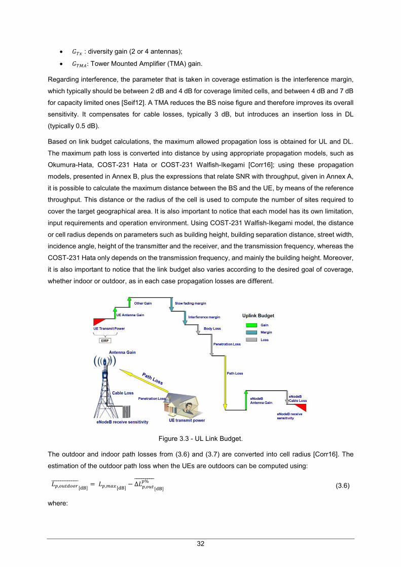
32

�� : diversity gain (2 or 4 antennas);

��: Tower Mounted Amplifier (TMA) gain.

Regarding interference, the parameter that is taken in coverage estimation is the interference margin,

which typically should be between 2 dB and 4 dB for coverage limited cells, and between 4 dB and 7 dB

for capacity limited ones [Seif12]. A TMA reduces the BS noise figure and therefore improves its overall

sensitivity. It compensates for cable losses, typically 3 dB, but introduces an insertion loss in DL

(typically 0.5 dB).

Based on link budget calculations, the maximum allowed propagation loss is obtained for UL and DL.

The maximum path loss is converted into distance by using appropriate propagation models, such as

Okumura-Hata, COST-231 Hata or COST-231 Walfish-Ikegami [Corr16]; using these propagation

models, presented in Annex B, plus the expressions that relate SNR with throughput, given in Annex A,

it is possible to calculate the maximum distance between the BS and the UE, by means of the reference

throughput. This distance or the radius of the cell is used to compute the number of sites required to

cover the target geographical area. It is also important to notice that each model has its own limitation,

input requirements and operation environment. Using COST-231 Walfish-Ikegami model, the distance

or cell radius depends on parameters such as building height, building separation distance, street width,

incidence angle, height of the transmitter and the receiver, and the transmission frequency, whereas the

COST-231 Hata only depends on the transmission frequency, and mainly the building height. Moreover,

it is also important to notice that the link budget also varies according to the desired goal of coverage,

whether indoor or outdoor, as in each case propagation losses are different.

Figure 3.3 - UL Link Budget.

The outdoor and indoor path losses from (3.6) and (3.7) are converted into cell radius [Corr16]. The

estimation of the outdoor path loss when the UEs are outdoors can be computed using:

��,��[��]

= ��,��[��] − ∆��,��

�%��[��]

(3.6)

where:

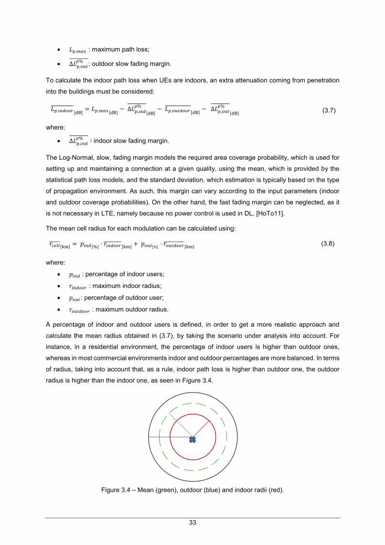
33

��,�� : maximum path loss;

∆��,��%��: outdoor slow fading margin.

To calculate the indoor path loss when UEs are indoors, an extra attenuation coming from penetration

into the buildings must be considered:

��,��[��]

= ��,��[��]− ∆��,��

�%��[��]

− ��,��[��]

− ∆��,��%��

[��] (3.7)

where:

∆��,��%�� ∶ indoor slow fading margin.

The Log-Normal, slow, fading margin models the required area coverage probability, which is used for

setting up and maintaining a connection at a given quality, using the mean, which is provided by the

statistical path loss models, and the standard deviation, which estimation is typically based on the type

of propagation environment. As such, this margin can vary according to the input parameters (indoor

and outdoor coverage probabilities). On the other hand, the fast fading margin can be neglected, as it

is not necessary in LTE, namely because no power control is used in DL, [HoTo11].

The mean cell radius for each modulation can be calculated using:

��[��]

= ��[%]⋅��

[��]+ ��[%]

⋅��[��]

(3.8)

where:

�� : percentage of indoor users;

�� : maximum indoor radius;

��: percentage of outdoor user;

�� : maximum outdoor radius.

A percentage of indoor and outdoor users is defined, in order to get a more realistic approach and

calculate the mean radius obtained in (3.7), by taking the scenario under analysis into account. For

instance, in a residential environment, the percentage of indoor users is higher than outdoor ones,

whereas in most commercial environments indoor and outdoor percentages are more balanced. In terms

of radius, taking into account that, as a rule, indoor path loss is higher than outdoor one, the outdoor

radius is higher than the indoor one, as seen in Figure 3.4.

Figure 3.4 – Mean (green), outdoor (blue) and indoor radii (red).

34

3.1.4 Capacity Planning

After the site coverage area is calculated, capacity related issues are analysed. With a rough estimate

of the cell size and site count, a verification of coverage analysis is carried out for the required capacity.

If the coverage estimate for the given configuration fulfils capacity requirements, then, there is no

addition to the previous plan; on the opposite, a suitable number of cell sites is added to achieve capacity

targets. After computing the cell range, the number of users inside the cell can be calculated from:

��,��[��]= �[��/��²]·�[��] (3.9)

where:

� : user density in the target area;

� : maximum area of coverage obtained.

The network dimensioning process is based on the assumption of a uniform distribution of users inside

the coverage area. The number of users for each modulation corresponds to a percentage of the total

one calculated in (3.9), taking the obtained radius for each modulation into account, a validation being

done by the following expression, Figure 3.5:

��,�� = ��,�� + ��,�� + ��,�� (3.10)

where:

��,�� =��

�

�� ·��,��

��,�� =��

�

�� ·��,��

��,�� =��

�� ·��,��

Figure 3.5 - Uniform distribution of users.

Furthermore, another factor that affects capacity requirements is the user traffic demands and the trend

of each user type. It is well known that traffic distribution is not uniform, i.e., there are always cells that

capture more traffic and reach their capacity limits much sooner than others, and that others usually

operate at a lower traffic demand. For this reason, the traffic demand distribution regarding the provided

35

services and certain services at the busies types of the day are factors that are taken into account. Thus,

in order to estimate the number of users that a single eNB can support and the average traffic load that

it can hold, the information on possible different traffic types and their parameters is essential, i.e., the

service mix, or service profile, which is given by the number of active users in a specific service and the

total number of active users. With an assumption of user response and market trend, the service mix

can be roughly estimated. Moreover, three different traffic types are considered: Residential, Office and

Mixed. As such, the traffic of each user is considered to determine if the maximum permissible network

load is exceeded, according to these three traffic profiles.

Then, capacity planning gives an estimate of the radio resources needed for supporting a specific

offered traffic with a certain quality, [Syed09]. As previously detailed, the total number of RBs in a cell is

fixed, usually taking the 2600 MHz carrier with a maximum number of 100 RBs, while the 1800 MHz

with 75 RBs, and the 800 MHz with 50 RBs, meaning that each band has a bandwidth of 20 MHz,

15 MHz, and 10 MHz, respectively. The available channel bandwidth is very important for capacity

planning, because it is directly connected to the capacity of the base station; the higher the bandwidth,

the more traffic it can support. So, in order to evaluate the capacity of each band, it is important to

analyse the average number of RBs that are requested by a single user for each service. In terms of

capacity, the throughput per RB is obtained through the model in Figure 2.7, from which the respective

average numbers for each modulation are estimated, taking the maximum and minimum throughputs

for each modulation into account. For QPSK, the minimum value depends on the reference throughput;

since the average throughput per RB is higher for higher order modulations, the number of required RBs

for a user is lower for 64-QAM than for QPSK for the same service and respective throughput. Therefore,

the average number of required RBs per user for each service and modulation can be obtained from:

��,��,�� = �

��,��,��[��]

��,��

[��]

� (3.11)

where:

��,��,�� : average throughput per user of a service s;

��,�� : average throughput per RB of each modulation n.

From the total number of active users, a certain percentage of users corresponds to each modulation

as shown in Figure 3.5, based on (3.10), hence, the number of required RBs is calculated for each

modulation taking the provided services into account. The number of RBs obtained for each modulation

is different, since the average throughput per RB and number of users in each of them is different,

therefore, the total number of RBs required for each modulation can be obtained from:

��,�� = � ��,��,�

�� ∙��,�� ∙��,�[%]

��

(3.12)

where:

��,�� ∶ number of served users by modulation n;

��,� : subscriber usage percentage of a service s.

36

Finally, the total number of RBs required for a single cell can be obtained from:

��,�� = �� + ��

�� + �� (3.13)

where:

��: number of RBs required in QPSK;

��: number of RBs required in 16-QAM;

��: number of RBs required in 64-QAM.

Seven types of services are considered for DL and four for UL. The number of covered users obtained

from (3.8) and number of active (or served) users’ needs to be equal when the system is coverage-

limited, as all covered users are spending resources in the network in a specific time instance. Thus,

��,�� assumes an important role in capacity planning, because it determines if the system is

coverage- or capacity-limited. If ��,�� exceeds the total number of RBs in a cell defined by

available channel bandwidth, the network is considered capacity-limited and, consequently, the average

throughput per cell and number of active users are reduced, as can be seen in Figure 3.6.

Regarding the definition of overload, one can use a generic formulation, by dividing the total available

resources in a cell by the quantity of required resources. Moreover, the total number of RBs in a cell is

fixed, therefore, one can use (3.14) to determine the respective cell capacity ratio:

�� = ��,��

��,��

(3.14)

where:

��,�� : total number of required RBs in the respective cell;

��,��: total number of RBs in the respective cell.

This value ranges from 0 to 1, with 1 indicating that a given cell is still limited by coverage. �� is used

only when the total number of RBs in the cell is exceeded. When a cell is not overloaded, i.e,. the total

number of RBs required is less than the total number of RBs in a cell, �� takes a value of 1 in (3.14).

The total average throughput of a cell can be obtained from:

��,��[��]

= � ��,��,��[��]

��

∙��,� ∙ �� (3.15)

where:

��,� : Number of active users in the service s.

The total throughput of the network obtained in (3.15) corresponds to the sum of the offered bit rate of

all served users. The percentage of traffic that each service occupies in the network (traffic profile), is:

��[%]=��,��,��

[��]∙��,� ∙ ��

��,��[��]

(3.16)

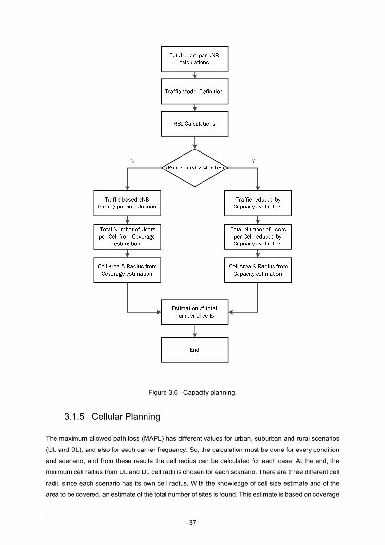
37

Figure 3.6 - Capacity planning.

3.1.5 Cellular Planning

The maximum allowed path loss (MAPL) has different values for urban, suburban and rural scenarios

(UL and DL), and also for each carrier frequency. So, the calculation must be done for every condition

and scenario, and from these results the cell radius can be calculated for each case. At the end, the

minimum cell radius from UL and DL cell radii is chosen for each scenario. There are three different cell

radii, since each scenario has its own cell radius. With the knowledge of cell size estimate and of the

area to be covered, an estimate of the total number of sites is found. This estimate is based on coverage

38

requirements and needs to be verified for capacity requirements. So, after determining the cell radius

for each scenario, the cell coverage area is calculated for an assumed cell structure or type. The cell

structure can be circular or hexagonal. Both are ideal representations, where circular cells give a simple

analysis and hexagonal ones give a best fit coverage site without any overlap and gaps. However, no

handovers occur between cells taking hexagons’ regularity, hence, a percentage for handover has to

be defined, which is used to reduce the maximum radius obtained from capacity or coverage

evaluations, so that handovers between cells can occur. One assumes a hexagonal cell structure, where

the cell area depends on the site configuration, being calculate, for a tri-sectorised site, as:

��=

3

2⋅√3 ⋅�[��]

� (3.17)

where:

� : maximum radius from coverage or capacity estimation.

The number of sites to be deployed can be easily calculated from the cell area and the deployment one:

�� = ��

��[��] � (3.18)

where:

�� : studied area of deployment.

The total number of cells is one of the main objects of study along the considered network, while other

important parameters, such as the cell radius from coverage or capacity evaluation and the number of

RBs allocated in each carrier frequency and in each type of service, are also analysed so that it is

possible to optimise the main outputs of the dimensioning process.

3.2 Model Implementation

The models described in Section 3.1 were implemented using a simulator developed with the C# (C

Sharp) programming language, which was adapted from the simulator supplied by the partner company.

Although the simulator was not done from scratch, it was restructured and based on work developed in

previous theses, such as [Guit16], followed by alterations under the scope of this thesis. This

dimensioning tool is designed to carry both coverage and capacity calculations. It performs the required

calculations, providing the site count on the basis of traffic forecast as the final result. The work

previously developed in this simulator considers only LTE, using a snapshot approach, where results

refer to the behaviour of the network at a given time instant, being like a “snapshot” of the busy hour

traffic. As one can see in Figure 3.7, the simulator workflow is represented by three main types of blocks,

with rounded purple corresponding to the modules where the user actually interacts with and inserts the

input parameters. All input data corresponds to the scenario under analysis, regarding information about

the environment and the coverage and capacity requirements. All the inputs can be entered in one class,

‘techDim.cs’, the purpose being to allow users to easily change dimensioning inputs in one place.

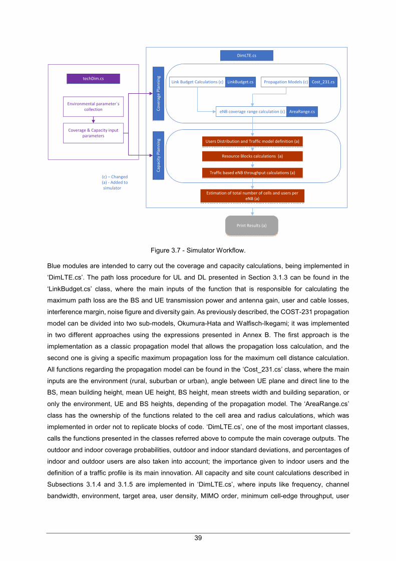
39

Environmental parameter´s collection

Coverage & Capacity input parameters

(c) – Changed(a) - Added to simulator

Link Budget Calculations (c) Propagation Models (c)

eNB coverage range calculation (c)

Users Distribution and Traffic model definition (a)

Estimation of total number of cells and users per eNB (a)

Print Results (a)

LinkBudget.cs Cost_231.cs

AreaRange.csCo

vera

ge P

lan

nin

gC

apac

ity

Pla

nn

ing

DimLTE.cs

techDim.cs

Resource Blocks calculations (a)

Traffic based eNB throughput calculations (a)

Figure 3.7 - Simulator Workflow.

Blue modules are intended to carry out the coverage and capacity calculations, being implemented in

‘DimLTE.cs’. The path loss procedure for UL and DL presented in Section 3.1.3 can be found in the

‘LinkBudget.cs’ class, where the main inputs of the function that is responsible for calculating the

maximum path loss are the BS and UE transmission power and antenna gain, user and cable losses,

interference margin, noise figure and diversity gain. As previously described, the COST-231 propagation

model can be divided into two sub-models, Okumura-Hata and Walfisch-Ikegami; it was implemented

in two different approaches using the expressions presented in Annex B. The first approach is the

implementation as a classic propagation model that allows the propagation loss calculation, and the

second one is giving a specific maximum propagation loss for the maximum cell distance calculation.

All functions regarding the propagation model can be found in the ‘Cost_231.cs’ class, where the main

inputs are the environment (rural, suburban or urban), angle between UE plane and direct line to the

BS, mean building height, mean UE height, BS height, mean streets width and building separation, or

only the environment, UE and BS heights, depending of the propagation model. The ‘AreaRange.cs’

class has the ownership of the functions related to the cell area and radius calculations, which was

implemented in order not to replicate blocks of code. ‘DimLTE.cs’, one of the most important classes,

calls the functions presented in the classes referred above to compute the main coverage outputs. The

outdoor and indoor coverage probabilities, outdoor and indoor standard deviations, and percentages of

indoor and outdoor users are also taken into account; the importance given to indoor users and the

definition of a traffic profile is its main innovation. All capacity and site count calculations described in

Subsections 3.1.4 and 3.1.5 are implemented in ‘DimLTE.cs’, where inputs like frequency, channel

bandwidth, environment, target area, user density, MIMO order, minimum cell-edge throughput, user

40

requested throughput per service, percentages of service usage (service mix) and percentage profiles

of user traffic for UL and DL, are also taken into account.

A lot of effort was put into the change of the existing implementation, in order to get a more realistic

approach of the network´s behaviour. Considering link budget calculations and propagations models,

as well as the possibility to have both outdoor and indoor users, and throughput calculation based on

the expressions provided in Annex A, a more realistic approach in capacity planning based on the

service usage distribution was implemented from scratch (highlighted in red in Figure 3.7). Some other

changes were also made, since only LTE is considered; as such, legacy parameters related to other

systems were removed from the simulator, in order to reduce running time and get a more efficient

approach – the simulator was restructured to accommodate the changes introduced in this thesis.

In order to typify the list of errors from the development of the code for the radio dimensioning, two

classes were created: ‘Strings_Reference.cs’ and ‘Return_Object.cs’. The former does not contain any

method, only global public variables, in order to centralise and typify the error messages in one place.

The latter only contains three public variables, referring to ‘Name’, ‘Value’ and ‘Error’. The “Print Results”

module corresponds to the block where the generated output files are. In order to create an Excel file

with its outputs, it was necessary to create a class called ‘Results.cs’.

In the last module, “Print Results”, some output files are created:

DimLTECoverage-DL.csv: mean indoor and outdoor cell radii, for each modulation, and the

maximum coverage area, for DL.

DimLTECapacity-DL.csv: cell area and radius obtained from capacity estimation, taking the

handover rate into account, for DL.

DimLTEOutputs-DL.csv: main output parameters of the dimensioning process, i.e., number of

cells of each district, cell radius, number of active users per cell, and average throughput per

cell regarding the services used by active users in each district, for DL.

DimLTECapacity-UL.csv: the same information as DimLTECapacity-DL.csv, but for UL.

DimLTEOutputs-UL.csv: the same information as DimLTEOutputs-DL.csv, but for UL.

DimLTEOutputs-Tot.csv: basically, the same information as DimLTEOutputs-DL.csv or

DIMLTEOutputs-UL.csv, depending on which link has a higher number of cells.

After the introduction of all parameters, a preliminary study on coverage is done, where the coverage

area for each of the frequency bands is calculated. It is based on a reference minimum throughput,

which is translated into a minimum SINR via (A.2), taking into account that, at the cell edge, QPSK is

the modulation scheme being used, as it is the most robust one, enabling realistic throughputs at a

relatively low SINR. When the throughput increases the distance decreases, until the maximum defined

for each modulation is achieved, and vice versa. The maximum cell distance calculation approach was

developed through reverse engineering the appropriate propagation model described in Annex B. As a

starting point for this approach, a specific maximum propagation loss allowed between the BS and the

UE has to be given as input. This propagation loss is obtained at a first stage by the classic link budget

procedure, taking noise power into account where the calculated SINR is translated into a minimum

41

received power, being then possible to extract the maximum cell radius for each modulation and carrier

frequency through the reversed model.

At this moment, the total number of covered users in a single cell is computed from (3.9), being uniformly

distributed regarding the maximum radius of each modulation, as seen in Figure 3.5. Each cell has a

number of RBs dictated by the bandwidth being considered, according to Table 2.2. Users are given all

the RBs they need in order to receive the maximum throughput associated with the service they are

requesting, if radio channel conditions support it; at this step, system capacity is not taken into account.

UEs demand different numbers of RBs, taking the received SINR into account. Bad SINR conditions

that correspond in most cases to a higher number of used RBs for a given throughput, and vice-versa.

Taking into account the uniform distribution of users, it is possible to verify that, for the same provided

service, a user in QPSK requires more RBs than one in 64 QAM.

In order to able to calculate the number of RBs that a user needs in order to fulfil the desired data rate,

the throughput for a single RB is calculated based on the model in Figure 2.7, with an average value for

each modulation. Resource allocation is done on an RB basis instead of on a sub-frame one, since the

simulator is snapshot based. The user´s desired throughput is divided by the throughput for a single RB

(being picked the integer ceiling value), in order to have knowledge, in a first approach, of the number

of RBs requested by the user.

Considering that the minimum allocation unit is the resource block and the average throughput per RB

is around 200 kbps in QPSK, there will be a huge difference between the offered and the processed

capacity for voice service. Voice is a service with an average bit rate of 12.2 kbps, the resource allocation

does not need to be performed every time-slot, instead being processed every 20 ms. This means that

the number of active voice users is computed by dividing the number of covered voice users by 20.

The simulator checks if the number of RBs required by users is lower than the maximum number of RBs

in a cell, the system being considered coverage-limited in this case, otherwise it is considered capacity-

limited. After the calculation of RB, based on user´s requested throughput, it is checked if those are

coherent with the network capacity; if no reduction has to occur, users are not requesting more

resources than the ones the network is able to provide them; if required, a reduction is carried out via

(3.14), where, in a first approach, the requested throughput is decreased until the capacity limit is

achieved. At this stage all cells are in their capacity limits.

To conclude, when the system is coverage-limited, the cell radius is not initially changed, but only when

the handover percentage is multiplied to the obtained radius, with a reduction of the radius being done

according to the defined handover percentage (usually around 95%). The number of coverage cells is

then calculated by (3.18). If the number of required RBs for the active users is higher than maximum, a

reduction of the number of users in the cell is verified, thus forcing the radius to decrease. The cell radius

obtained is divided by the maximum area of coverage (being picked the integer floor value), in order to

have knowledge of the number of users supported by single a cell. After the multiplication of the obtained

capacity radius by the same handover percentage, the number of capacity cells can be determined, as

seen in Figure 3.6. It is important to notice that the obtained number of cells corresponds to the number

of sites needed to fulfil all requirements. As previously mentioned, all sites are considered tri-sectorised.

42

Finally, some Excel files are automatically created with the output values, serving as a tool to study and

compare the number of cells for different traffic scenarios and different carrier frequencies. All files are

generated for each simulation, containing the results for a specific combination of the input parameters.

An extension to the simulator, to study UL dimensioning using the same methods as in DL, was also

implemented. The main difference between the two links is the number and type of required services

and throughput associated with them. Usually, the user´s requested throughput for UL is lower than DL.

3.3 Model Assessment

During model development, in order to validate its implementation, the obtained results were subjected

to a set of empirical tests. A careful examination off all variables and formulas was made, in order to

check if they were coherent and also accurate from a theoretical viewpoint. Some intermediate and

different tests were carefully chosen to cover all calculations done by the implementation of both model

approaches, which are detailed in Section 3.2. The results of the simulation, as previous discussed,

were saved in Microsoft Excel files, which enabled a more efficient validation of some tests, such as the

cell radius from coverage or capacity evaluation and, consequently, the number of cells in UL and DL,

as well as the total number of active users supported by a single cell.

A list with the most critical tests performed for the coverage model approach is provided in Table 3.1.

Table 3.2 presents a list with tests made for the capacity model approach.

Table 3.1 - List of empirical tests performed to validate the implementation of the coverage model.

Test Validation

1 Check if an error message is shown after all input parameters are inserted.

2

Validation of the link budget and propagation models calculations: using a scientific

calculator to compute some specific intermediate values and compare them with the ones

obtained in the simulator.

3 Verify if the minimum path loss between UL and DL is chosen.

4 Verify if the radius of each cell in the 3 frequency bands varies according to different input

parameters.

5 Verify if the cell radius is decreasing with the increase of modulation order.

6 Check if the number of coverage cells increases with the increase of frequency band.

7 Check if the .xlsx output file, with the coverage outputs results, exists and is located in the

Output Directory.

43

Table 3.2 - List of empirical tests performed to validate the implementation of the capacity model.

Test Validation

1 Check if an error message is shown after all input parameters are inserted.

2

Validation of the number of RBs requested by a user in each service: using a scientific

calculator to compute some specific values and compare them with the ones obtained in

the simulator.

3 Verify if the number of active users and total number of users per cell are equal when the

total number of RBs is lower than the maximum number of RBs that can be served in a cell.

4 Check if the percentage of active users per cell decreases with the increase on the total

number of users when the system is capacity-limited.

5 Verify if the total number of cells increases with the increase on the total number of users.

6 Verify if the total number of cells, for the same channel bandwidth, increases with the

increase of frequency band.

7 Check if all .xlsx output files exist and are located in the Output Directory.

To check the accuracy of the simulator, in terms of number of cells for a certain area, a number of

simulations as done, varying the user density as well as the available channel bandwidth. The number

of cells for 2600 MHz is expected to be higher than for the two other carrier frequencies for the same

channel bandwidth, as shown in Figure 3.8. The channel bandwidth is 20 MHz for the three carrier

frequencies. In the simulation with the highest frequency, one can conclude that while the network is

limited by coverage, the number of cells remains constant. However, one can verify that the network

load is exceeded with an increase in the number of cells, from the moment that the number of required

RBs exceeds the allowed maximum being verified. Furthermore, it is important to notice that all

simulations were tested for different environments and scenarios, but, for reasons of simplicity, in these

simulations the Lisbon area with an urban environment was considered.

Figure 3.8 – Number of cells versus User density.

0

100

200

300

400

500

600

10 20 30 40 50

Nu

mb

er o

f ce

lls/1

00

km

2

Number of Users/km2

800 MHz

1800 MHz

2600 MHz

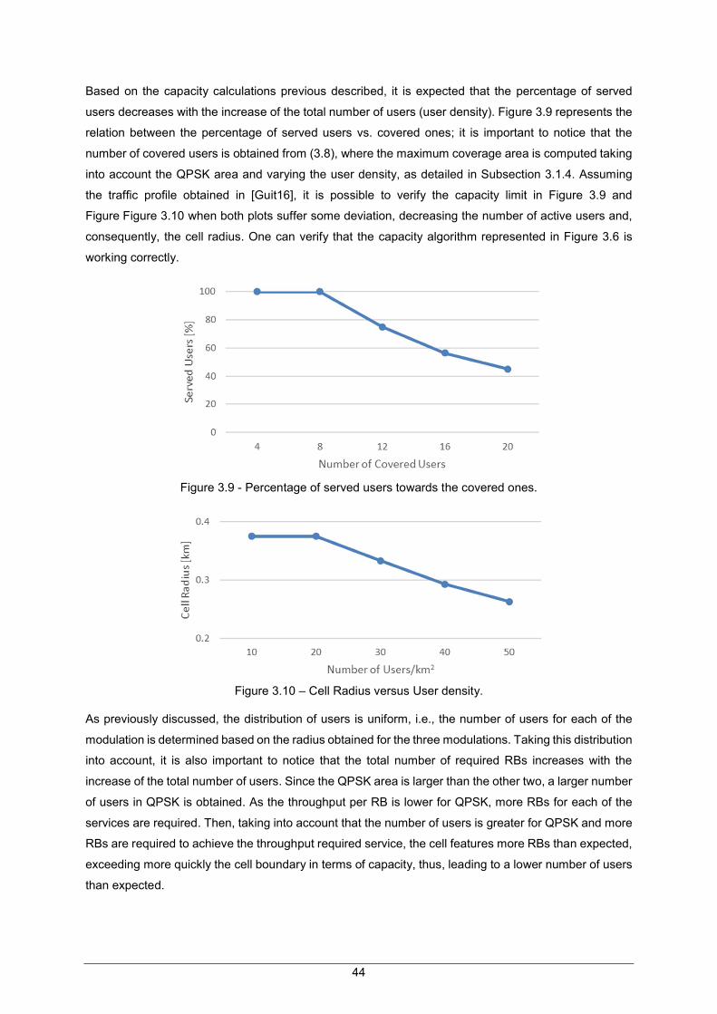
44

Based on the capacity calculations previous described, it is expected that the percentage of served

users decreases with the increase of the total number of users (user density). Figure 3.9 represents the

relation between the percentage of served users vs. covered ones; it is important to notice that the

number of covered users is obtained from (3.8), where the maximum coverage area is computed taking

into account the QPSK area and varying the user density, as detailed in Subsection 3.1.4. Assuming

the traffic profile obtained in [Guit16], it is possible to verify the capacity limit in Figure 3.9 and

Figure Figure 3.10 when both plots suffer some deviation, decreasing the number of active users and,

consequently, the cell radius. One can verify that the capacity algorithm represented in Figure 3.6 is

working correctly.

Figure 3.9 - Percentage of served users towards the covered ones.

Figure 3.10 – Cell Radius versus User density.

As previously discussed, the distribution of users is uniform, i.e., the number of users for each of the

modulation is determined based on the radius obtained for the three modulations. Taking this distribution

into account, it is also important to notice that the total number of required RBs increases with the

increase of the total number of users. Since the QPSK area is larger than the other two, a larger number

of users in QPSK is obtained. As the throughput per RB is lower for QPSK, more RBs for each of the

services are required. Then, taking into account that the number of users is greater for QPSK and more

RBs are required to achieve the throughput required service, the cell features more RBs than expected,

exceeding more quickly the cell boundary in terms of capacity, thus, leading to a lower number of users

than expected.

45

Chapter 4

Results Analysis

4 Results

Analysis

This chapter provides a description of the reference scenario used in the simulations along with the

obtained results and their respective analysis.

46

4.1 Scenarios Description

The reference scenario is the city of Lisbon and its surrounding areas. In Figure 4.1, the total area

studied in the simulator is represented, which is divided into different municipalities with a different

variety of users’ density, and amount of generated traffic, meaning that each zone has different coverage

and capacity requirements. It is important to notice that each municipality is divided into districts; as

such, the model uses a granularity at the level of districts, each of the granular areas being classified

according to one of the considered geotypes (urban, suburban and rural), which are defined according

to the population density of each district. This approach leads the urban environment to be characterised

by a high proportion of population, the contrary occurring for the rural environment. Therefore, the main

output, i.e., the number of cells, is obtained for each district. The total number of cells of each

municipality is obtained from the sum of the number of cells for each of the districts that belong to the

municipality.

Figure 4.1 – Reference user density in the Lisbon City and its surrounding areas.

This region has an area of approximately 1500 km2, where, as expected, the majority of the population

is concentrated in the city. The percentages of urban and suburban scenarios were estimated to be 11%

and 26%, respectively, and the remaining 63% for rural. The population density of Lisbon is not the

highest, as seen in Figure 4.2.

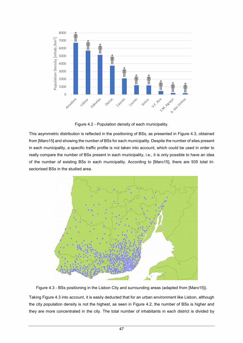
47

Figure 4.2 - Population density of each municipality.

This asymmetric distribution is reflected in the positioning of BSs, as presented in Figure 4.3, obtained

from [Maro15] and showing the number of BSs for each municipality. Despite the number of sites present

in each municipality, a specific traffic profile is not taken into account, which could be used in order to

really compare the number of BSs present in each municipality, i.e., it is only possible to have an idea

of the number of existing BSs in each municipality. According to [Maro15], there are 935 total tri-

sectorised BSs in the studied area.

Figure 4.3 - BSs positioning in the Lisbon City and surrounding areas (adapted from [Maro15]).

Taking Figure 4.3 into account, it is easily deducted that for an urban environment like Lisbon, although

the city population density is not the highest, as seen in Figure 4.2, the number of BSs is higher and

they are more concentrated in the city. The total number of inhabitants in each district is divided by

0

1000

2000

3000

4000

5000

6000

7000

8000

Po

pu

lati

on

Den

sity

[in

hab

./km

2]

48

district area (being picked the integer value), in order to know, in a first approach, the population density

in each district. After that, the population density obtained of each district is multiplied by penetration

and usage ratios. Using a snapshot approach, the real number of subscribers (instant active users) is

used in capacity calculations. The penetration ratio corresponds to the percentage of users with

smartphone internet access, while the usage ratio corresponds to the percentage of users who are

enjoying some service at the instant of time under study. In the reference scenario, the penetration ratio

is 15% and the usage one is 10%, but these values were changed in order to compare the total number

of cells. The user densities presented in Figure 4.2 were obtained taking those ratios into account. The

number of inhabitants for each district were obtained in [Stat16] and the area of each district in [Dire16].

It has been explained in the previous chapter that the path loss depends on coverage probability,

interference margin and path loss model. Signal propagation fading determines the total attenuation

level, and, as a result, the fading margin for each fading type, indoor and outdoor, is assumed as shown

in Table 4.1 andTable 4.2, respectively. Fast fading was not taken into account, also as explained

before.

Table 4.1 – Indoor Mean and Standard Deviation for each frequency band (extracted from [Corr16]).

Band [MHz] Average [dB] Standard deviation [dB]

800 2.6 9.2

1800 10.2 13.8

2600 13.6 15.9

Table 4.2 – Parameters for the reference scenario.

Parameter Description Value

Reference throughput [Mbps] 2.0

Outdoor coverage probability [%] 90.0

Outdoor standard deviation [dB] 6.0 / 8.0

Indoor coverage probability [%] 90.0

Indoor Users [%] 70.0

Outdoor Users [%] 30.0

Penetration Ratio [%] 15.0

Usage Ratio [%] 10.0

Handover percentage [%] 95.0

In indoor and outdoor propagation, a statistical approach was used in order to compute the

corresponding slow fading margin, i.e., the Log-Normal Distribution, giving the penetration attenuation

for a given overall coverage probability. The differences found in slow fading are a consequence of the

49

standard deviation: in rural and suburban areas, the standard deviation is lower than in urban ones,

hence, two different values being used, Table 4.2; the standard deviations in urban areas with highly

integrated buildings layout and deeper indoor coverage is higher than in a suburban environment, the

outdoor standard deviation being based on [Tele13] while the indoor one being defined for each

frequency band, as seen in Table 4.1. In the dimensioning process, indoor or outdoor scenarios were

taken, and it was considered that 70% of users are indoor and 30% are outdoor. This comes from the

fact that nowadays, with a subscription of data plans, users consume more data services indoors, during

work time, at the mall, or at home. The outdoor scenario corresponds to users that are walking on

streets, and, for that reason, an extra attenuation was not considered. The indoor path loss is then

higher than the outdoor one, and, consequently, the outdoor distance is greater than the indoor one.

The analysis of the outputs has been done taking the DL scenario into account, considering three

different frequency bands associated with their maximum available bandwidths:

800 MHz with a bandwidth of 10 MHz, which provides coverage;

1800 MHz and 2600 MHz with a bandwidth of 20 MHz, which provide extra capacity.

The values presented in Table 4.3 are based on [Guit16], with the exception of the noise figure, diversity

gain, interference margin and TMA gain, which were defined taking into account the values presented

in [LTEE16]. UEs of Category 3 (which are able to support DL throughputs up to 100 Mbps) with a 2x2

MIMO configuration were considered, with an EPA5 channel.

Table 4.3 - Simulation Parameters.


Frequency Bands [MHz] 800 1800 2600

Maximum Bandwidth [MHz] 10.0 20.0 20.0

DL transmission power [dBm] 42.0

BS maximum antenna gain [dBi] 17.8

Modulations QPSK,16QAM, 64QAM

UE antenna gain [dBi] 0

UE losses [dB] 1.0

Cable losses [dB] 2.0

Noise figure [dB] 5.0 (UL) / 8.0 (DL)

Diversity gain [dB] 3.0

Interference margin [dB] 3.0

TMA gain [dB] 2.0

MIMO order [dB] 2.0

50

As mentioned before, path loss is calculated using the COST 231 Walfish-Ikegami or COST 231

Okumura Hata models, presented in Annex B, and the parameters shown in Table 4.4: the former for

both urban and suburban scenarios, and the latter for rural ones; the values for the parameters were

based on [Guit16] for the urban environment; for the suburban and rural environments, the height of the

BS antennas was increased compared to the urban environment, the width of the streets and the

distance between the centre of the buildings was reduced for the suburban environment, taking into

account the differences of the terrain morphology between urban and suburban environments. The UE

height corresponds to the average holding height of the UEs for both data and voice usage.

Table 4.4 - Configuration of parameters for the propagations models.


Environment Urban Suburban Rural

Height of the BS antennas (ℎ�) [m] 25.0 28.0 30.0

Height of the buildings (��) [m] 21.0 21.0 -

Street width (��) [m] 30.0 20.0 -

Distance between building centre (��) [m] 50.0 30.0 -

Incidence angle (� ) [°] 90

UE height (ℎ�) [m] 1.2

Simulations were performed for 7 types of services for DL, i.e., voice (VoLTE), video calling, video and

music streaming, web browsing, file sharing and e-mail, and 4 for UL, i.e., voice, video calling, file

sharing and e-mail. Each one has minimum, average and maximum throughputs; however, the average

throughput per user for the higher throughput services had to be adapted taking into account that the

throughput values presented in [Guit16] were too demanding. Regarding voice, it was taken as VoLTE,

as it is already under commercial implementation [Voda15]. The service mix was extracted from [Guit16],

where the considered device is a smartphone. As one can see in Table 4.5, video streaming and web

browsing use the majority of the resources, since with the current success of smartphones, the different

sorts of internet based services incorporated in them, and also the effect of social networks, users are

driven to use internet based services such as video and music streaming more often than other services.

Social networking is evaluated as web browsing, so these two types of services were taken jointly. Users

were also categorised as residential, office or mixed, based on their service requirement and traffic load

that they place in terms of usage; as such, the service mix of each traffic profile is different according to

the area and time instance under study. However, for the reference scenario, all users were considered

as residential, hence, the service mix presented in Table 4.5 - Services characteristics (adapted from

[Guit16]) is associated with a residential profile, where video streaming predominates. A study was done

taking the three traffic profiles into account, where the percentages of services are changed according

the type of user, i.e., the distribution of users considers the three variants in order to make a more

realistic approach.

51

Table 4.5 - Services characteristics (adapted from [Guit16])

Service Service Class Average Bit Rate [Mbps] Service Mix [%]

VoLTE Conversational 0.022 22

Video Calling Conversational 0.384 8

Streaming Streaming 2 28

Music Streaming Streaming 0.196 20

Web Browsing Interactive 2 10

File Sharing Interactive 2 8

E-mail Background 1 4

As a first analysis, the impact on the number of cells for each municipality was studied, changing the

total number of users. In this study, it is easily seen that the largest number of users the higher the

amount of required cells to fulfil coverage and capacity requirements. Secondly, some variations for

other inputs were performed. In the reference scenario, the frequency band and respective maximum

bandwidth used are 1800 MHz and 20 MHz, respectively; however, the band and the bandwidth was

varied, in which three cases were compared to the reference scenario, all of them at 10 MHz, 15 MHz

and 20 MHz. Also, the impact of changing the minimum reference throughput was studied, as well as

the services throughput, presented in Table 4.5. Regarding the input parameter service mix, one

compared the network performance on the change in the percentage of each service. Two different

service profiles were tested, adapted from those proposed by [Alme13] and [Ganc15], comparing the

required number of cells for each scenario. In order to analyse what is the impact of the input parameters

on the main output ones and extract conclusions, a variation of the former was done. All the analysed

input and output parameters are presented in Figure 4.4, with purple and grey boxes, respectively.

Figure 4.4 - List of analysed Input and Output parameters.

In order to provide a classification of the reference area as urban, suburban and rural, an approximation

was considered, based on the number of users in each area. The areas with a high concentration of

users were considered as urban or suburban, opposite to the case of rural ones, where the concentration

of users is lower. In order to simplify the process, the areas corresponding to each environment are

52

outlined in Figure 4.5. Taking the area of each district into account, obtained in [Dire16], and the

respective classification in terms of environment, the total area of each environment was computed.

Figure 4.5 – Division of the reference area into environments (adapted from Google Maps).

Figure 4.6 represents the number of cells of each municipality obtained in simulations. Since each

municipality has a number of districts with different areas and population densities, and consequently

user densities, the user density and area of each district, presented in Annex C, are essential to compute

these results, considering also the other parameters defined for the reference scenario. Taking the traffic

profile presented in Table 4.5 into account, a total of 1243 BSs were obtained. As expected, the number

of cells in Lisbon is higher, being reduced for the rural areas, since users’ density is very low compared

to urban areas.

Figure 4.6 – Number of cells for each municipality taking the reference parameters into account.

Each environment is associated with a set of districts, and the number of sites presented in Figure 4.7

0

50

100

150

200

250

300

350

400

Lisbon Sintra Cascais Loures Oeiras Amadora Odivelas V.F. Xira Mafra S.M.Agraço

A. dosVinhos

Nu

mb

er o

f C

ells

53

for each scenario was obtained by considering the sum of the required number of cells of each district

in order to fulfil the coverage and capacity requirements defined in the reference scenario. In Figure 4.7,

one can observe the number of cells per 10 km2 for each environment; the number of urban cells is

higher than the one for suburban and rural areas, as expected.

Figure 4.7 - Number of cells per 10 km2 for each environment.

For each district, a number of sites with a certain radius was determined, Figure 4.8 showing the average

cell radius obtained for each environment. As mentioned in the previous chapter, the maximum allowed

path loss (MAPL) has different values for urban, suburban and rural. In terms of coverage, considering

that a higher path loss corresponds a lower maximum cell radius, it is of no surprise that, for the urban

environment, the mean cell radius is lower than for the suburban or rural ones, as seen in Figure 4.8,

where for each analysis the average value of the studied parameter is presented, as well as the

corresponding standard deviation of each simulation on the top of each bar. Taking these facts into

account, it is necessary to have more urban cells than suburban and rural ones to fulfil coverage

requirements. In terms of capacity, when increasing the user density more resources are required and

the probability of the cell being limited by capacity is greater. When the cell is overloaded, the cell radius

decreases in order to fulfil capacity requirements. For that reason, and considering that most of the

obtained cells are limited by capacity, more cells are needed in areas with a higher user density. This

fact can be confirmed by the number of cells presented in Figure 4.7.

Regarding cell radius, it is also verified that the average cell radius for the suburban scenario is slightly

lower than the expected. This result can be explained by the definition of some of the propagation model

parameters for the suburban environment, such as, BS antenna height, street width and building

separation, but also by the fact that the environment classification of the districts is an approximation,

as can be seen in Figure 4.8. Although some districts present a considerable reference user density,

some of them were considered suburban taking their location into account. For this reason, the cell radii

of those districts are lower than the ones obtained for most of suburban districts. As such, the average

cell radius in suburban environment decreases in relation to the expected radius.

0

5

10

15

20

25

30

35

Urban Suburban Rural

Nu

mb

er o

f ce

lls /

10

km

2

Scenario

54

Figure 4.8 – Average cell radius for each environment.

4.2 Analysis on the Number of Users

In a first approach, the impact of varying the total number of users on the network performance was

studied, regarding the number of active users that is obtained considering the application of the

penetration and usage ratios in the total number of inhabitants in each district. For this analysis, as one

can see in Table 4.6, only three different combinations were done. It is easily seen that increasing both

ratios lead to an increase of users’ density.

Table 4.6 - Penetration and Usage Ratio for each scenario.

Scenario Penetration Ratio [%] Usage Ratio [%]

Reference 15 10

Double 30 20

Triple 45 30

The algorithm provides RBs to users until there are no RBs left to be allocated. If a cell is overloaded,

there must be a reduction in the number of RBs down to the limit allowed by the bandwidth. The total

number of used RBs depends on the traffic profile of active users: if the traffic profile is heavier, i.e. the

average throughput per user established for each of the services is too demanding in terms of capacity,

it is seen that by increasing the number of active users in the network, more traffic is generated, thus,

more RBs will be used. As previously discussed, a cell is limited by capacity when the number of RBs

used by active users is higher than the maximum of available RBs, while, if after fulfilling the capacity

requirements for all active users there are still available RBs, one considered that it is coverage-limited.

0

0.5

1

1.5

2


Cel

l Rad

ius

[km

]

Scenario

55

In the reference scenario, the services with the highest percentage of use are web browsing and video

streaming. These services have the highest throughput, and therefore consume most of the available

resources, thus leading to a higher percentage of cells limited by capacity.

Furthermore, increasing the population density means that users’ density increases as well,

independently of the area, which can be translated into a decrease in the cell radius and in the number

of active users if the network is limited by capacity, leading to an increase in the number of cells, as one

can see in Figure 4.9. When the cells of a district are limited by coverage, the cell radius and the number

of active users remain constant. For the reference scenario, it is expected that the number of urban cells

is higher than for the other two types of environments. Comparing the results from Figure 4.9, it is

concluded that the number of urban cells is higher for the three defined scenarios due to the fact that

the urban area presents a higher user density.

Figure 4.9 – Number of cells per 10 km2 for different scenarios taking users’ density into account.

When the penetration and usage ratios double the users’ density quadruples, and when both ratios triple

the users’ density increases nine-fold. An interesting conclusion to be drawn from Figure 4.9 is that the

number of cells increases proportionally with the number of active users.

4.3 Bandwidth and Frequency Band Analysis

In this section, the behaviour with the variation of the bandwidth in each band is analysed, for each case,

the total number of cells required to cover the target area being presented. Varying the frequency band

results in a change in the path loss used to calculate the maximum cell radius, resulting in different

coverage areas. BSs having different coverage areas originate different network configurations, hence,

the capacity limit does not change in a linear way.

Considering the propagation models’ parameters that depend on the type of environment, the maximum

0

50

100

150

200

250

300

350


Nu

mb

er o

f ce

lls /

10

km

2

Reference

Double

Triple

56

obtained cell radii for urban environments are lower than the ones obtained for suburban and rural

environments. As seen in Table 4.7, for the same environment, the maximum obtained cell radius is

higher for the lowest frequency and lower for the highest frequency, as expected, since the 800 MHz

band has a lower path loss compared to the others.

Table 4.7 – Maximum radius of a cell for different bands.

Frequency

Band [MHz] Environment

Cell Radius

[km]

800

U 1.91

S 2.19

R 15.12

1800

U 0.58

S 0.79

R 6.80

2600

U 0.31

S 0.49

R 5.00

In terms of capacity, one can distribute the scenarios in ascending order by All 10 MHz, All 15 MHz, All

20 MHz, where each frequency is associated with all bandwidths, as can be seen in Figure 4.10. When

the bandwidth varies, the percentage of RBs guaranteed at the cell edge also varies; as previously

mentioned, the percentage taken as a reference is 10.0%, but when the bandwidth decreases, for the

same percentage the minimum throughput per RB exceeds the maximum defined for QPSK. The

solution is to increase the percentage of guaranteed RBs at the cell edge when the bandwidth

decreases, therefore, for 15 MHz the defined percentage was 13.3%, and for 10 MHz the percentage

was 20.0%, to ensure that the minimum RB throughput does not exceed the allowed maximum.

Although greater bandwidths correspond to more available resources, and considering that the

reference traffic profile is ambitious compared with the service throughputs required by users in reality,

most cells remain limited by capacity. With the increase in available bandwidth, the network can provide

more resources for services, meaning that the lower the bandwidth, the higher is the required number

of cells, as shown in Figure 4.10, for the same frequency band. When comparing the three bands, it is

seen that the number of cells for the highest frequency is higher than the other two, assuming that the

bandwidth is equal for all bands. It was expected that, with the increasing frequency, the number of cells

would increase. As seen in Figure 4.10, the number of cells obtained for the 800 MHz band is very

similar to the one for 1800 MHz, considering that the bandwidth is equal, which is explained by the fact

that capacity is the dominating factor, as less resources are available for these bands and the reference

traffic profile is too demanding. However, the number of cells for 1800 MHz is always higher than the

800 MHz one, as expected.

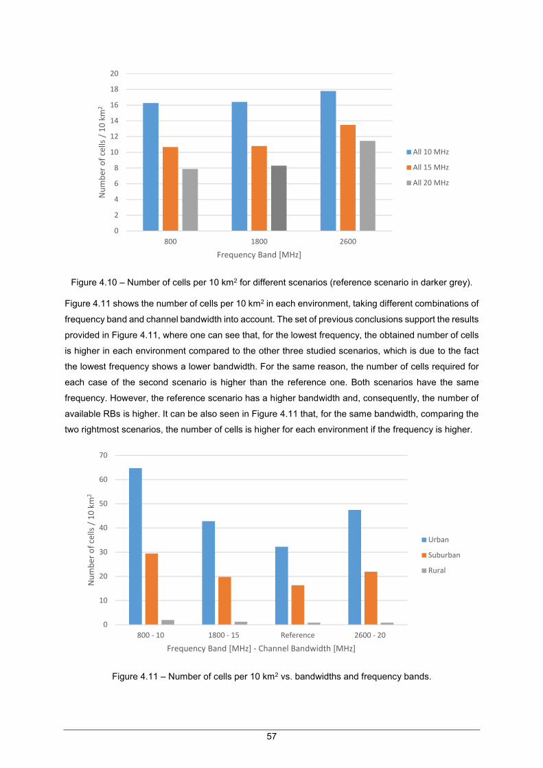
57

Figure 4.10 – Number of cells per 10 km2 for different scenarios (reference scenario in darker grey).

Figure 4.11 shows the number of cells per 10 km2 in each environment, taking different combinations of

frequency band and channel bandwidth into account. The set of previous conclusions support the results

provided in Figure 4.11, where one can see that, for the lowest frequency, the obtained number of cells

is higher in each environment compared to the other three studied scenarios, which is due to the fact

the lowest frequency shows a lower bandwidth. For the same reason, the number of cells required for

each case of the second scenario is higher than the reference one. Both scenarios have the same

frequency. However, the reference scenario has a higher bandwidth and, consequently, the number of

available RBs is higher. It can be also seen in Figure 4.11 that, for the same bandwidth, comparing the

two rightmost scenarios, the number of cells is higher for each environment if the frequency is higher.

Figure 4.11 – Number of cells per 10 km2 vs. bandwidths and frequency bands.

0

2

4

6

8

10

12

14

16

18

20

800 1800 2600

Nu

mb

er o

f ce

lls /

10

km

2

Frequency Band [MHz]

All 10 MHz

All 15 MHz

All 20 MHz

0

10

20

30

40

50

60

70

800 - 10 1800 - 15 Reference 2600 - 20

Nu

mb

er o

f ce

lls /

10

km

2

Frequency Band [MHz] - Channel Bandwidth [MHz]

Urban

Suburban

Rural

58

4.4 Analysis on Coverage Percentages

Since radio coverage is based on probabilities, indoor and outdoor coverage at a specific location from

a BS can be specified for 50%, 90%, or even a higher probability. The slow fading margin is the “safety

factor” used to determine the level of probability of successful radio communication. The higher the

fading margin, the higher the probability that a usable communication signal is received, and the smaller

the coverage area required to fulfil it. The previous statements support the results provided in Table 4.8,

where the cells with higher probability present a lower radius.

Table 4.8 – Variation of the cell radius vs. outdoor and indoor coverage percentages.

District Environment

Cell Radius [km]

Coverage Estimation Capacity Estimation

85 % Reference 95% 85% Reference 95%

Ericeira S 0.912 0.781 0.630 0.908 0.781 0.630

Loures S 0.912 0.781 0.630 0.908 0.781 0.630

Alcabideche S 0.912 0.781 0.630 0.816 0.781 0.630

Belém U 0.697 0.579 0.579 0.644 0.579 0.579

Cascais U 0.697 0.579 0.579 0.618 0.579 0.579

Sintra I S

0.912 0.781 0.630 0.912 0.781 0.630 Sintra II S

V. Pinheiro S

As already mentioned, one of the determining aspects in the characterisation of cells is that the users’

density is limited by coverage or capacity. If the density of users is low, the probability of being in the

presence of cells limited by coverage is greater, depending on the traffic profile associated with users.

As such, an area may have a low users’ density, but if the users’ traffic profile is very demanding, the

probability of capacity predominance is higher. Considering the reference traffic profile presented in

Table 4.5, it was possible to identify some suburban and urban districts in which cells are limited by

coverage. In this section, the main objective is to understand the impact on the number of cells and

whether the cells remain limited by the coverage, when the percentages of indoor and outdoor coverage

are changed. The analysis is based only on districts that are constituted by cells limited by coverage,

because it is possible to better understand the variation of coverage percentages on the required

number of cells. When cells are limited by capacity, the obtained number of cells is equal for each one,

even when varying the coverage percentages. For reasons of simplicity, the percentages of indoor and

outdoor coverage are changed with the same value; these changes were done in the same simulation

for each district limited by coverage.

With the increase of the percentage of outdoor and indoor coverage, the number of cells increases, as

seen in Figure 4.12. All the districts presented in Figure 4.12 are constituted by sites limited by coverage

59

for 90% (reference) and 95%; however, it comes down to 85%, some districts have capacity-limited

cells, with the reduction of the cell radius. This comes from the fact that the cell radius from coverage

estimation is higher for 85%, hence, the number of active users is also higher, so the number of required

RBs is higher, exceeding the maximum number of RBs allowed in the cell. As seen in Table 4.8, three

districts maintain the cell radius, while in the remaining ones there is decrease of the cell radius caused

by capacity. However, the path loss and, consequently, the cell radii are higher when both coverage

percentages are lower, so when both percentages are higher, more cells are needed in order to fulfil the

defined requirements, as seen in Figure 4.12.

Figure 4.12 – Number of cells for each district vs. outdoor and indoor coverage percentages.

In Figure 4.12, Sintra appears twice due to the fact that the district of Sintra is subdivided into three sub-

districts, two of them considered as suburban and one as rural. The districts presented in Figure 4.12

are the two suburban ones, as seen in Annex C. Sintra I and Sintra II correspond to Santa Maria and

São Miguel) and to São Pedro de Penaferrim, respectively.

Usually, the users’ density is low in rural areas, but in the reference scenario none of the rural districts

appears in the set of districts whose cells are limited by coverage, since the cell radius for rural

environments (and, consequently, the cell area) is significantly higher than in the other environments.

By multiplying the obtained rural area by the user density existing in the rural districts, the total covered

users number in the cell is obtained, being higher than that verified in other environments. Considering

the reference traffic profile for rural areas, the number of RBs to satisfy all active users is very large, and

for this reason rural cells are generally limited by capacity.

4.5 Traffic Profiles Analysis

For the analysis of traffic profiles, a scenario was chosen in which users have different traffic profiles.

While at the beginning, all users have only one traffic profile, residential, from now on two other types

0

5

10

15

20

25

30

35

40

45

Nu

mb

er o

f ce

lls

District

85%

Reference

95%

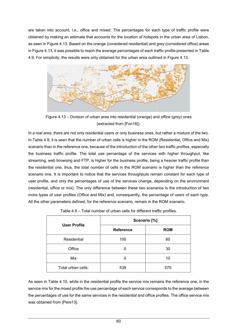
60

are taken into account, i.e., office and mixed. The percentages for each type of traffic profile were

obtained by making an estimate that accounts for the location of hotspots in the urban area of Lisbon,

as seen in Figure 4.13. Based on the orange (considered residential) and grey (considered office) areas

in Figure 4.13, it was possible to reach the average percentages of each traffic profile presented in Table

4.9. For simplicity, the results were only obtained for the urban area outlined in Figure 4.13.

Figure 4.13 – Division of urban area into residential (orange) and office (grey) ones

(extracted from [Fon16]).

In a real area, there are not only residential users or only business ones, but rather a mixture of the two.

In Table 4.9, it is seen that the number of urban cells is higher in the ROM (Residential, Office and Mix)

scenario than in the reference one, because of the introduction of the other two traffic profiles, especially

the business traffic profile. The total use percentage of the services with higher throughput, like

streaming, web browsing and FTP, is higher for the business profile, being a heavier traffic profile than

the residential one, thus, the total number of cells in the ROM scenario is higher than the reference

scenario one. It is important to notice that the services throughputs remain constant for each type of

user profile, and only the percentages of use of the services change, depending on the environment

(residential, office or mix). The only difference between these two scenarios is the introduction of two

more types of user profiles (Office and Mix) and, consequently, the percentage of users of each type.

All the other parameters defined, for the reference scenario, remain in the ROM scenario.

Table 4.9 – Total number of urban cells for different traffic profiles.

User Profile Scenario [%]

Reference ROM

Residential 100 60

Office 0 30

Mix 0 10

Total urban cells: 539 570

As seen in Table 4.10, while in the residential profile the service mix remains the reference one, in the

service mix for the mixed profile the use percentage of each service corresponds to the average between

the percentages of use for the same services in the residential and office profiles. The office service mix

was obtained from [Pere13].

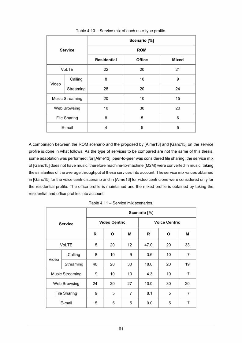
61

Table 4.10 – Service mix of each user type profile.

Service

Scenario [%]

ROM

Residential Office Mixed

VoLTE 22 20 21

Video Calling 8 10 9

Streaming 28 20 24

Music Streaming 20 10 15

Web Browsing 10 30 20

File Sharing 8 5 6

E-mail 4 5 5

A comparison between the ROM scenario and the proposed by [Alme13] and [Ganc15] on the service

profile is done in what follows. As the type of services to be compared are not the same of this thesis,

some adaptation was performed: for [Alme13], peer-to-peer was considered file sharing: the service mix

of [Ganc15] does not have music, therefore machine-to-machine (M2M) were converted in music, taking

the similarities of the average throughput of these services into account. The service mix values obtained

in [Ganc15] for the voice centric scenario and in [Alme13] for video centric one were considered only for

the residential profile. The office profile is maintained and the mixed profile is obtained by taking the

residential and office profiles into account.

Table 4.11 – Service mix scenarios.

Service

Scenario [%]

Video Centric Voice Centric

R O M R O M

VoLTE 5 20 12 47.0 20 33

Video Calling 8 10 9 3.6 10 7

Streaming 40 20 30 18.0 20 19

Music Streaming 9 10 10 4.3 10 7

Web Browsing 24 30 27 10.0 30 20

File Sharing 9 5 7 8.1 5 7

E-mail 5 5 5 9.0 5 7

62

A real network needs to adapt to the new specifications according to different service profiles. It is also

important to understand the network utilisation per user profile type, as, for instance, the behaviour of

voice calls peak hour might be very different from data ones. Network traffic is typically a mix of various

profiles that are weighted as a function of time and geographical area. This means, for instance, that

the office usage profile is weighted at city centres during working hours, while the residential one is

strengthened in urban areas during the evening. As such, two scenarios were established, one focused

more on video streaming and another on voice, in order to analyse the impact on the number of cells

when the service profile varies and to compare the results obtained with the reference service profile.

As seen in The service mix values obtained in [Ganc15] for the voice centric scenario and in [Alme13]

for video centric one were considered only for the residential profile. The office profile is maintained and

the mixed profile is obtained by taking the residential and office profiles into account.

Table 4.11, the traffic profile is changed according to the scenario, and it can be seen that, in the profile

focused on video streaming, the percentage is higher than in the ROM reference. As for the profile

focused on voice, the percentage is also higher than the one established as reference. Since video

streaming requires more RBs than voice, taking the higher associated average throughput per user into

account, it can be concluded that the number of urban cells is greater for the traffic profile where the

video is predominant, as seen in Figure 4.14. Consequently, for the ROM profile, the number of cells is

higher than the required number of cells for the profile where voice is predominant, as for the last profile

service percentages are less demanding in terms of capacity. Increasing the percentage of the most

demanding services in terms of capacity, the number of cells needed to fulfil all requirements increases.

It is also verified that substantially increasing the percentage of voice does not result in an increase in

the number of cells compared to the ROM scenario, because the services that require more resources

suffer a decrease in their percentage of use, reinforcing the previous ideas.

Figure 4.14 – Number of urban cells per 10 km2, for different service profiles scenarios.

A comparison between the reference scenario and the ones proposed by [Guit16] on the traffic profile

is performed next. As the average throughput required by the user is too demanding for some of the

services considered in this thesis, there was a need to adapt the values for some services, namely for

0

5

10

15

20

25

30

35

40

45

50

Voice Centric ROM Video Centric

Nu

mb

er o

f ce

lls /

10

km

2

Scenario

63

the services with the highest throughput. The remaining services present the throughput values

presented in [Guit16]. The main objective is to understand the impact, in terms of the number of cells,

when the throughput required by the users for all services is increased or decreased; two traffic profiles

have been created, Lower and Higher, in order to make a comparison with the throughputs defined as

reference. Previously, it was the service mix that changed depending on the scenario, now it is the

throughput that each user requires for each service that changes, maintaining the service mix.

Table 4.12 – Throughput values for the studied scenarios.

Service Bit Rate [Mbps]

Lower Reference Higher

VoLTE 0.009 0.022 0.036

Video Calling 0.231 0.384 0.422

Streaming 1 2 4

Music Streaming 0.176 0.196 0.294

Web Browsing 1 2 4

File Sharing 1 2 4

E-mail 0.819 1 1.5

Figure 4.15 shows the number of urban cells per 10 km2 for each of the established scenarios. As

expected, it is seen that the scenario with a heavier traffic profile in terms of throughput has more cells,

while the scenario with a lighter traffic profile presents fewer cells. The reason for this is also associated

with the increase of the required RBs in order to satisfy the higher throughputs requested by users. With

a heavier traffic profile, capacity prevails over coverage, and the cells’ radius decreases, hence, more

cells are needed in order to satisfy capacity requirements.

Figure 4.15 – Number of urban cells per 10 km2 for each scenario.

0

10

20

30

40

50

60

70

Lower ROM Higher

Nu

mb

er o

f ce

lls /

10

km

2

Scenario

64

4.6 Impact of Reference Throughput Analysis

In this section, the main purpose is to analyse the impact on the number of cells when the required

throughput at the cell edge is changed. From the reference throughput, the throughput per RB is

computed taking into account the percentage of guaranteed RBs at the cell edge. For this study, a

couple of scenarios were proposed in order to compare with the obtained number of cells for the

reference throughput, 2 Mbps. It was verified that there is a limitation with respect to values above

2 Mbps, since the obtained throughput per RB is always higher than the maximum throughput per RB,

for QPSK, taking the reference percentage of RBs (10%) into account at the cell edge. Changing this

percentage, as in the bandwidth analysis, can be done by lowering the throughput per RB until the

maximum of QPSK is reached; however, the throughput per RB is equal to the one obtained for the

ROM scenario, adding no value to the results, as such only the study for 1Mbps and 2 Mbps was made.

The change in the throughput value is directly related to distance, since with the increase of throughput,

the distance decreases and vice versa, i.e., the higher the reference throughput, the higher the

throughput per RB and, consequently, the lower the cell radius. Therefore, when decreasing the cell

radius more cells are needed for the highest reference throughput, i.e., 2 Mbps, which is not verified.

When the number of cells is obtained for the 1 Mbps scenario, it is possible to verify a limitation at the

level of the implemented model, considering that the obtained number of cells is higher in comparison

with the ROM reference, which is not expected, but rather the opposite. Considering that the scenario

with lower throughput is associated with a lower throughput per RB, it is possible to conclude that the

cell radii obtained for this scenario are greater, and consequently the number of cells is smaller or equal,

never higher, in comparison with the number of the ROM scenario one.

Considering the scenario with lower throughput, and the fact that cells are mostly limited by capacity for

each district, the obtained radii are always lower than the ones obtained for the ROM scenario, which is

not correct. This comes from the fact of the average throughput per RB is smaller than the reference

one, thus, the number of RBs required for each service is higher, leading to a higher overload of the

cell. It is a fact that, for the scenario with lower throughput, the maximum obtained cell radius is higher

than the one for the ROM scenario, in terms of coverage; however, when capacity is taken into account,

the radii of the cell from capacity estimation are lower than the ones in the ROM scenario, hence, the

need for the implementation of the condition, so as to not contradict theory.

In order to solve this limitation, the following condition was imposed: when the throughput per RB is less

than the maximum defined for QPSK, 200 kbps, and the obtained radius decreases due to capacity, the

calculations are made according to the maximum throughput, so that the scenario with the lowest

throughput does not present a radius smaller than the one obtained for the ROM scenario. Given this

solution, the number of cells for each of the scenarios is equal, as a consequence from the fact that the

maximum throughput matches the average throughput per RB for the scenario of 2 Mbps and the

obtained cell radii, for each district, are equal in each scenario.

65

Chapter 5

Conclusions

5 Conclusions

This chapter summarises all the work carried out, and the main conclusions are presented. In the end,

one gives a few recommendations for future work.

66

The main purpose of this thesis was to study the dimensioning and planning processes in an LTE

network deployed over different scenarios, in order to understand the impact on the number of cells of

the network when some of the input parameters vary. In order to accomplish this goal, a model was

developed and several simulations were performed, analysing the impact of different user densities,

areas, bandwidths, services throughputs, and the services percentages on the network performance.

The region of Lisbon was chosen as a reference scenario, as it presents different municipalities with

different varieties of user density and, considering that most of the data were collected from previous

theses based on the same area, the definition of the inputs of the model became more accessible.

Simulations were done for each district with different number of active users distributed along the

network using either typical data download services or VoLTE.

The first chapter of this thesis is intended to briefly describe mobile communications evolution over time,

followed by a short explanation of the growing data traffic demands, and finally addressing the motivation

and contents that lead to the development of this thesis.

In Chapter 2, the theoretical background on LTE´s fundamental aspects is presented, concerning

network architecture, radio interface, coverage and capacity aspects, and services and applications.

Also, a description of some traffic services is presented, to help define the different types of traffic

considered in this work. At the end of this chapter, a brief description of the state of the art on the thesis

subject is provided, presenting some of the previously developed works that tackle dimensioning models

and methods.

Chapter 3 starts by presenting the models that were developed in the scope of this thesis, as well as

the simulator that implements them. The simulator addresses, in the most realistic way possible, the

reality of an LTE network, considering aspects such as target area, different traffic profiles and different

user density according to the zone of the municipality. Users, as a rule, are distributed non-uniformly

over the entire target area, however, in this thesis, the network dimensioning process is based on the

assumption of uniform distribution of users within the coverage area. This assumption has a limitation

in terms of capacity, as the number of users is always higher for QPSK, as the QPSK area obtained is

higher. In QPSK, more RBs are required to ensure the throughput of a service required by a user than

in the other modulations, thus, the total number of RBs obtained for QPSK is higher as expected, taking

into account that there are more users than in other modulations. However, the cell features more RBs

than expected, exceeding more quickly the cell capacity limit, thus, leading to a lower number of users

than expected. Moreover, in order to calculate the received power, a link budget taking only the slow

fading margin into account is used. For the calculation of path loss, the COST 231 Walfisch-Ikegami

and COST Okumura Hata models were considered according to the environment, as described in Annex

B. Expressions for throughput calculation of each UE are presented in Annex A. Moreover, the whole

process of traffic load calculation was implemented from scratch, to satisfy different service demands,

while always taking the load of each cell into account. In the last part of the chapter, a model assessment

is provided, confirming that the number of cells increases with the increase of user density, and that

when cells are limited by capacity the cell radius and the number of active users inside the cell decrease.

When the number of required RBs exceeds the maximum allowed for each bandwidth, the higher the

67

number of RBs required to satisfy the traffic profile, the lower the cell radius and consequently the

number of active users. It is important to refer that the traffic studied under the scope of this thesis is

only in downlink.

Chapter 4 starts by describing the reference scenario considered in this thesis, considering all

parameters used in the simulator, as well as the set of input and output parameters to be analysed. The

three frequency bands used by Portuguese mobile operators in LTE are used in this thesis; each of

them has an associated bandwidth that usually depends on the carrier frequency. The lower the

frequency band, the higher the costs, since lower frequency bands are better for providing a larger

coverage area. The antennas parameters were chosen taking a given antenna as reference, and,

although only the 1800 MHz band is used, with a bandwidth of 20 MHz, in the reference scenario, the

other two frequency bands were also used in the results analysis, because they have particular

characteristics worthwhile exploiting: different path loss (due to different frequencies), thus different

coverage, and different available bandwidth, thus different capacities. Three different environments

were considered for the region of Lisbon: urban, suburban and rural. The differences between the three

environments are essentially based on different parameters for the propagation model, as well as user

density. The result analysis includes the variation of the number of users, different frequency bands and

bandwidths, coverage probabilities and, finally, the variation in the services throughputs and service mix

taking different user profiles into account.

In the analysis of the impact of the number of users on the number of cells, three different combinations

of penetration and usage ratios are taken. Each combination corresponds to a single scenario. In the

double scenario, both ratios doubled compared to the reference, while in the triple scenario they triple.

These ratios are applied to the total number of inhabitants of each district, in order to compute the users’

density in each of the districts. It is easily seen that, by increasing both ratios, the users’ density also

increases. When the user density increases, the load in cells also increases, as the cell radius and the

number of active users follow the opposite trend when the cells are capacity-limited, therefore, it can be

concluded that the obtained number of cells increases when the users’ density increases. As expected,

the obtained number of cells for the reference scenario is lower than for the other scenarios. Considering

that the user density quadruples when the ratios double and user density increases nine times when the

ratios triple, it is also verified that the total number of cells quadruples and increases nine-fold compared

to the obtained number of cells for the reference scenario, in double and triple scenarios, respectively.

Varying the bandwidth of each band has impact on the obtained number of cells and cell radius. In terms

of cell radius, it is concluded that, for the lower frequency, the associated path loss is lower and,

consequently, the maximum cell radius is also higher. As such, in terms of coverage, the required

number of cells to cover a given area, for the lowest frequency, is lower. With the increase in available

bandwidth, the network can provide more resources for services, meaning that the lower the bandwidth,

the higher the required number of cells, for the same frequency band and traffic profile, and vice-versa.

For instance, the obtained number of cells for the scenario with the combination (1800 MHz,15 MHz)

increases by 33% over the reference scenario. Assuming that the available bandwidth is equal for all

frequency bands, it is also verified that, for the higher frequency, the obtained number of cells is higher.

68

In fact, for the scenario with the combination (2600 MHz, 20 MHz), the number of cells increases by

47% over the reference scenario. However, it is possible to verify that, for the lower frequency and

bandwidth, in comparison with the reference scenario or the scenario with higher throughput and

bandwidth, the obtained number of cells is higher, given the available resources in each bandwidth.

For the indoor and outdoor coverage probabilities variation test, as expected, the impact is essentially

verified in the cell radius. When the coverage probability increases, the obtained cell radius decreases.

Decreasing the cell radius while maintaining the same traffic profile for each scenario, results in the

need for more cells for the scenario with a higher coverage probability. It is also interesting to verify that,

for the lower coverage probability, in some of the coverage-limited cell districts, these limitations switch

to capacity ones, while increasing the cell radii. Considering that the increase of the cell radius allows

the support of more users, the maximum capacity of the cell is reached, thus, a reduction of the radius

is verified.

All of the previous analysis was made considering only residential users for the different environments.

However, a distribution of users taking three different user profiles into account was developed in order

to have a more realistic approach of the behaviour of a real network. A further analysis considers also

this approach, where a percentage of residential, office and mixes users are defined. For simplicity, the

urban scenario was the only scenario chosen. The number of urban cells obtained for the ROM scenario

is higher than the one for the reference scenario. In fact, the number of cells for the ROM scenario

increases by 6% over the reference scenario, where all users are considered as residential, given the

introduction of two other profiles, especially the office profile, where higher service percentages for the

most demanding services is verified.

The reference service profile, with the three user profiles, is compared with the ones proposed by

[Alme13] (Video Centric) and [Ganc15] (Voice Centric). Video streaming is one of the most demanding

resource services, since it has the maximum throughput. Therefore, the cells load for this test is much

higher compared to the voice centric one. Obviously, the required number of cells for the scenario

focused more on video service is higher than the one for the other scenarios. The number of cells for

the video centric scenario increases by 30% over the ROM scenario. The obtained number of cells for

the voice centric scenario is lower than the one obtained for the ROM scenario, as the percentages of

the service mix of residential and mixed user profiles are lower for the services with higher throughput.

The number of cells for the voice centric scenario decreases about 12% over the ROM scenario.

For the services throughputs variation test, two scenarios were proposed in order to compare the

number of cells with the one obtained in the ROM scenario. As expected, the required number of cells

for the scenario with higher throughputs in all services is higher than the ones for the ROM scenario and

for the scenario with lower throughputs in all services. The number of cells for the scenario with higher

throughputs increases by 85% over the ROM scenario, whereas, for the scenario with lower

throughputs, the number of cells decreases about 41% over the ROM scenario. With higher throughputs,

capacity is the dominating factor, leading to a higher number of cells needed to fulfil the users’

requirements. Obviously, if services throughputs are not as demanding, the number of cells is lower.

69

For the analysis of the impact of the required throughput at the cell edge on the number of cells, a

scenario with lower throughput was analysed and some limitations regarding the implemented model

could be verified. At the beginning, for the scenario with lower throughput, the obtained radii were always

lower than the ones obtained for the reference scenarios, in terms of capacity. Consequently, the

obtained number of cells for the scenario with lower throughput was higher than the one obtained for

the ROM scenario with higher throughput at the cell edge, which is not correct. The reason for this is

associated with the throughput per RB used in the capacity calculations. Since it is smaller, more RBs

are allocated and, for this reason, the radius is reduced, requiring a higher number of cells. In terms of

coverage, the number of cells obtained for the scenario with lower throughput is lower than the one for

the ROM scenario, as expected. Theoretically, the number of cells should be equal or higher for the

ROM scenario. After the implementation of this condition, the obtained number of cells for both scenarios

was equal.

A real mobile communications network is far more complex than the one analysed in this wotk. Other

limitations of this work are related to the fact that neither the terrain profile or Lisbon’s very irregular

structure, which includes different buildings that may impose limitations to coverage areas and received

power levels, are considered.

A great effort has been made in order to complete this work, but, as with all projects, there is always

room for improvement and further enhancements. For future works that tackle a similar subject to the

one of this thesis, an even more realistic scenario could be applied. Although the handover process is

taken into account in this thesis, other limitation is interference coming from adjacent cells. Taking into

account that inter-cell interference, or even intra-cell interference, can restrict the overall network in

terms of throughput and spectral efficiency, especially for users located at the cell edge, interference

management techniques could also be studied for future works, in order to know if they improve or not

network performance in a real deployment. A better model of throughput as function of SINR could also

be studied by taking different modes and coding rates in each modulation into account.

Another topic which could be addressed as future work is the usage of new LTE-Advanced

functionalities, like Carrier Aggregation, where developments in terms of usage of different carrier

frequencies in co-located sites should also be taken into account. The principle with Carrier Aggregation

is to extend the maximum bandwidth by aggregating multiple carriers in order to improve network

capacity. The use of this technique corresponds to a huge advantage in terms of achievable

throughputs, since it should provide a better user experience by using two or more of these carriers to

serve a given user and, therefore, enabling it to achieve higher throughputs.

Although this thesis only addresses communication via DL, the UL connection should also be analysed.

It is also important to understand if and how mobile communications networks cope with challenging UL

traffic loads resulting from services like Internet of Things (IoT), cloud enabled technologies and social

networking. Even more so when taking into account that nowadays users are not only consumers of

data, but are also starting to be active producers of content. For that reason, UL traffic has started to

follow a growing trend, and today the asymmetry between DL and UL traffic is reduced.

70

Finally, the variation of other parameters, together with their implications on the subject under study,

should also be analysed in order to have a better assessment of network capabilities. Different antenna

configurations, such as another MIMO orders, transmitter output powers, antenna´s height and noise

figure, for each environment, should be considered, so that one can better understand how these

parameters can influence the required number of cells and how their variation can help in obtaining

better results.

71

Annex A

SINR versus Throughput

Annex A. SINR versus Throughput Erro! A origem da referência não foi encontrada.

The following annex provides an overview about the formulas that relate SINR and Throughput in LTE

for a given set of system configurations.

72

In order to establish a relationship between SINR and Throughput, three expressions were derived for

the three modulation types considered in both the uplink and the downlink: QPSK, 16-QAM and 64-

QAM. These expressions represent the logistic functions that provide the best fit approach to a set of

values collected by 3GPP based on throughput performance tests done by manufacturers, presented in

[3GPP11]. In order to have a more realistic approach of the behaviour of a real network, the three

modulation schemes are considered and each one is associated with the median value of the coding

rates obtained according to the Channel Quality Indicator (CQI) reported by the UE, resulting in coding

rates of 1/3 for QPSK, 1/2 for 16QAM and 3/4 for 64QAM. It is also important to refer that all users are

considered to follow the EPA5 channel model.

For QPSK modulation, coding rate of 1/3 and considering MIMO 2x2, throughput per RB and the

corresponding SINR can be given by:

��[��] =2.34201∙10�

14.0051+ ��.�� ∙�� (A.1)

�� [��] = −1

0.577897 ∙ ln�

2.34201∙10�

��[��]− 14.0051� (A.2)

For 16QAM modulation, coding rate of 1/2 and considering MIMO 2x2, throughput per RB and the


��[��] =47613.1

0.0926275+ ��.�� ∙�� (A.3)

�� [��] = −1

0.295838 ∙ ln�

47613.1

��[��]− 0.0926275� (A.4)

For 64QAM modulation, coding rate of 3/4 and considering MIMO 2x2, throughput per RB and the


��[��] =26405.8

0.0220186+ ��.�� ∙�� (A.5)

�� [��] = −1

0.24491 ∙ ln�

26405.8

��[��]− 0.0220186� (A.6)

73

Annex B

Propagation Models

Annex B. Propagation Models Propagation Models used in this thesis are described in this annex.

74

B.1 COST-231 Walfisch-Ikegami Model

This model allows one to estimate the path loss between the signal emitted by the eNB to an UE as

shown in Figure B.1.It is used when dealing with urban and suburban scenarios for distances shorter

than 5 km, and also distinguishes between two different propagation scenarios: Line of Sight (LoS) and

Non-Line of Sight (NLoS), according to [Corr16].

For LoS propagation in a street ( = 0), and d > 0.02 km, path loss is defined as:

��,��[��] = 42.6 + 26 ∙log��[��]� + 20 ∙log (�[��]) (B.1)

where:

�: distance between the eNB and the UE;

�: frequency of the signal being propagated.

For all other cases, path loss is defined as:

��,��[��] = ��[��]+ ��[��]+ ��[��], �� + �� > 0

��[��] , �� + �� ≤ 0 (B.2)

where:

��: free space propagation loss;

��: attenuation due to propagation from eNB to the last rooftop;

��: attenuation due to diffraction from last rooftop to the UE.

Being the path loss experienced in free space propagation defined as:

��[��] = 32.4 + 20·log��[��]� + 20 ·log (�[��]) (B.3)

The propagation from the eNB to the last rooftop experiences the following loss:

��[��] = ��[��]+ �� + �� ·log��[��]� + �� ·log��[��]� − 9 ·log (��[�]) (B.4)

where:

��: loss due to the height difference between rooftop and the antennas;

��: distance between building´s centre.

The loss due to the height difference between rooftop and the antennas is obtained from:

��[��] = �− 18 ·log�ℎ�[�]− ��[�]+ 1� , ℎ� > ��

0 , ℎ� > ��

(B.5)

in which:

ℎ�: height of the BS antenna;

75

��: height of the buildings.

Other correction factors are obtained from:

�� = �

18 , ℎ� > ��

18 − 15ℎ�[�]− ��[�]

��

, ℎ� ≤ �� (B.6)

�� = � −4 + 0.7�

�[��]

925− 1� , urban and suburban scenarios

− 4 + 1.5��[��]

925− 1� , dense urban scenarios

(B.7)

�� = �

54 , ℎ� > ��

54 − 0.8�ℎ�[�]− ��[�]� , � ≥ 0.5 �� ˄ ℎ� ≤ ��

54− 1.6�ℎ�[�]− ��[�]��[��] , � < 0.5�� ˄ ℎ� ≤ ��

(B.8)

Finally, the loss due to diffraction from the last rooftop to the UE is defined as:

��[��] = −16.9 − 10 ·log��[�]� + 10 ·log��[��]� + 20·log��[�]− ℎ�[�]� + ��[��] (B.9)

where:

��: street width;

ℎ�: UE height;

The loss due to diffraction from the last rooftop to the UE is given by:

��[��] = �

− 10.0 + 0.354�[°] ,0° < � < 35°

2.5 + 0.075��[°]− 35�, 35° < � < 55°

4.0 − 0.114��[°]− 55�, 55° < � < 90°

(B.10)

where:

φ: angle of incidence of the signals in the buildings, on the horizontal plane;

The validity range for some parameters of this model imposes that:

�[800, 2000] MHz

�[0.02, 5] km

ℎ�[4, 50] m

ℎ�[1, 3] m

The presented frequency range does not contain all the frequency bands studied in this thesis, therefore,

one should consider higher relative errors than expected. The standard deviation of the model takes

values in [4; 7] dB, and the error increases when ℎ� decreases relative to ��. Some of the parameters

used in this model are presented in Figure B.1. In the absence of specific values, the following are

recommended [Corr16]:

��[20,50] m

�� = �� / 2

� = 90°

��[�] = 3 ·(#��)+ ��[�]

76

where:

�� = � 3 , pitched 0 , flat

Figure B.1 - Parameters in the COST-231 Walfisch-Ikegami Model.

B.2 Okumura-Hata Model

This model assumes that there are no dominant obstacles between the BS and the MS, and that the

terrain profile changes only slowly. It is used when studying rural, suburban and urban environments for

distances larger than 5 km. The path loss for this model is described by:

�� [��] = 69.55 + 26.16log��[��]� − 13.82log�ℎ�[�]� + (44.9 − 6.55log(ℎ�[�]))��[��]�

− ��[��]− ��[��] (B.11)

where:

� ∶ frequency band;

ℎ� : effective height of BS antenna;

��: scenario correction factor;

� : distance between the BS and the UE;

�� [��] = �

�1.1 ·log��[��]� − 0.7�ℎ�[�]− (1.56·log��[��]− 0.8� , small city

8.29 ·(log (1.54 ·ℎ�[�])� − 1.10, � < 200 ��, large city

3.2 ·(log (11.75 ·ℎ�[�])� − 4.97, � ≥ 400 �ℎ� , large city

(B.12)

in which:

ℎ�: user equipment height;

77

�� [��] = �4.78 ·��(�[��])�

�− 18.33·log��[��]� + 40.98, rural scenarios

2 ·(log (�[��] /28))� + 5.4, suburban scenarios

0, urban scenarios

(B.13)

This model has a standard deviation for urban, suburban and rural environments approximated by:

� [��] = �0.70 ·log��

�(�[��])− 2.5 ·log��[��]� + 11.10, urban scenarios

0.98 ·log��(�[��])− 3.4 ·log��[��]� + 11.88, suburban and rural scenarios

(B.14)

and it is valid for the following values:

�[150, 1500] MHz

�[1, 20] m

ℎ�[30, 200] m

ℎ�[1, 10] m

It is noteworthy that the frequency range does not encompass the 1800 MHz and 2600 MHz frequency

range most commonly used for fourth generation cellular system. This problem was solved by the

COST-231 Hata Model, which extends the validity region to the 1.5-2 GHz range:

�� [��] = 46.3 + 33.9 ·log��[��]� − 13.82·log�ℎ�[�]� − ��[��]+ �44.9 − 6.55 ·log�ℎ�[�]��

·��[��]� − ��[��]+ ��[��] (B.15)

where:

��[��] = �0, small cities 3, urban centres

(B.16)

79

Annex C

Districts

Annex C Districts

This annex presents the geographical area, number of inhabitants, reference user density and the

considered environment (U – Urban, S – Suburban or R – Rural) for all districts defined for this thesis.

80

In this thesis, eleven municipalities were studied in the Lisbon region. As previously mentioned, each

municipality is divided by districts and the main output of this thesis, the number of cells, is obtained for

each district taking into account the values presented in the tables below. The area of each district was

obtained in [Dire16] and the number of inhabitants in [Stat16]. The reference user density was obtained

taking the reference penetration and usage rate into account. Therefore, all the studied municipalities

and its districts are detailed in the following tables:

Lisbon Municipality

Table C.1 - Lisbon Districts Characteristics.

District Environment Area [km2] Inhabitants Reference user

density [users/km2]

Ajuda U 3 15584 77

Alcântara U 4 13943 52

Alvalade U 5 31813 95

Beato U 2 12429 93

Benfica U 8 36821 69

Campolide U 3 15460 77

Carnide U 4 23316 87

Penha de França U 3 27967 139

Parque das Nações

U 5 21025 63

Estrela U 5 20128 60

Belém U 10 16528 24

Lumiar U 6 41163 102

Marvila U 7 38102 81

S.D. Benfica U 4 33745 126

São Vicente U 2 15339 115

Santo António U 1 11836 177

S.M. Maior U 3 12822 64

Santa Clara U 3 22480 112

Olivais U 8 33788 63

Misericórdia U 2 13044 97

Av. Novas U 3 21625 108

Arroios U 2 31653 237

Areeiro U 2 20131 150

Campo Ourique U 2 22120 165

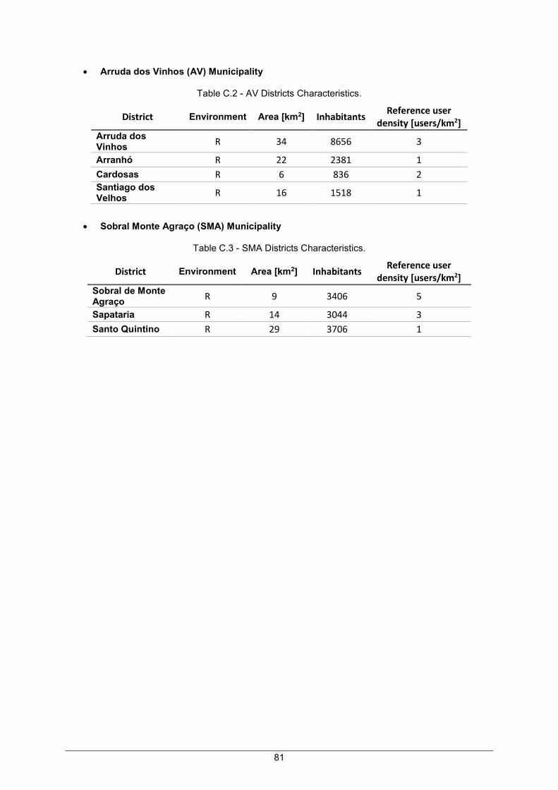
81

Arruda dos Vinhos (AV) Municipality

Table C.2 - AV Districts Characteristics.


density [users/km2] Arruda dos Vinhos

R 34 8656 3

Arranhó R 22 2381 1

Cardosas R 6 836 2 Santiago dos Velhos

R 16 1518 1

Sobral Monte Agraço (SMA) Municipality

Table C.3 - SMA Districts Characteristics.


density [users/km2] Sobral de Monte Agraço

R 9 3406 5

Sapataria R 14 3044 3

Santo Quintino R 29 3706 1

82

Sintra Municipality

Table C.4 - Sintra Districts Characteristics.


density [users/km2] Algueirão Mem Martins

S 16 66250 62

Almargem Bispo R 37 8983 3

Belas S 22 26087 17

Colares R 33 7628 3

Montelavar R 12 3559 4

Queluz S 3 26248 131

Rio de Mouro S 16 47311 44 Sintra (Santa Maria e São Miguel)

S 12 9364 11

S.J Lampas R 57 11392 2 Sintra (São Martinho)

R 24 6226 3

Sintra (São Pedro de Penaferrim)

S 27 14001 7

Terrugem R 23 5113 3

Pêro Pinheiro R 16 4246 3

Casal de Cambra S 2 12701 95

Massamá S 3 28112 140

Monte Abraão S 2 20809 156

Agualva S 8 35824 67

Cacém S 2 21289 159

Mira Sintra S 1 5280 79

S. Marcos S 2 17412 130

Cascais Municipality

Table C.5 - Cascais Districts Characteristics.


density [users/km2]

Alcabideche S 40 42162 15

Carcavelos U 5 23347 70

Cascais U 20 35409 26

Estoril U 9 26399 43

Parede U 4 21660 81

S.D. Rana S 20 57502 43

83

Odivelas Municipality

Table C.6 - Odivelas Districts Characteristics.


density [users/km2]

Caneças S 6 12324 30

Famões S 5 11095 33

Odivelas U 5 59559 178

O. Basto S 2 5812 43

Pontinha U 5 23041 69

P.S. Adrião S 1 13069 196

Ramada S 4 19657 73

Amadora Municipality

Table C.7 - Amadora Districts Characteristics.


density [users/km2]

Alfragide S 3 9904 49

Águas Livres S 2 37426 280

Encosta do Sol S 3 28261 141 Falagueira - V. Nova

S 3 23186 115

Mina de Água S 8 43927 82

Venteira s 5 18539 55

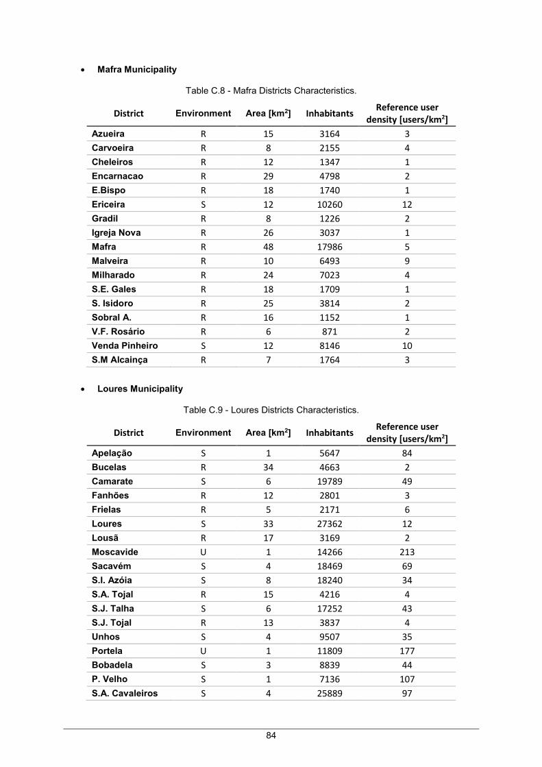
84

Mafra Municipality

Table C.8 - Mafra Districts Characteristics.


density [users/km2]

Azueira R 15 3164 3

Carvoeira R 8 2155 4

Cheleiros R 12 1347 1

Encarnacao R 29 4798 2

E.Bispo R 18 1740 1

Ericeira S 12 10260 12

Gradil R 8 1226 2

Igreja Nova R 26 3037 1

Mafra R 48 17986 5

Malveira R 10 6493 9

Milharado R 24 7023 4

S.E. Gales R 18 1709 1

S. Isidoro R 25 3814 2

Sobral A. R 16 1152 1

V.F. Rosário R 6 871 2

Venda Pinheiro S 12 8146 10

S.M Alcainça R 7 1764 3

Loures Municipality

Table C.9 - Loures Districts Characteristics.


density [users/km2]

Apelação S 1 5647 84

Bucelas R 34 4663 2

Camarate S 6 19789 49

Fanhões R 12 2801 3

Frielas R 5 2171 6

Loures S 33 27362 12

Lousã R 17 3169 2

Moscavide U 1 14266 213

Sacavém S 4 18469 69

S.I. Azóia S 8 18240 34

S.A. Tojal R 15 4216 4

S.J. Talha S 6 17252 43

S.J. Tojal R 13 3837 4

Unhos S 4 9507 35

Portela U 1 11809 177

Bobadela S 3 8839 44

P. Velho S 1 7136 107

S.A. Cavaleiros S 4 25889 97

85

Oeiras Municipality

Table C.10 - Oeiras Districts Characteristics.


density [users/km2]

Barcarena S 9 13869 23

Carnaxide S 7 25911 55

Oeiras U 7 33827 72

Paço de Arcos U 3 15315 76

Algés U 2 22273 167

Cruz Quebrada U 3 6393 31

Linda-a-Velha U 2 19999 149

Porto Salvo S 8 15157 28

Queijas S 2 10377 77

Caxias U 3 9007 45

Vila Franca de Xira (VFX) Municipality

Table C.11 - VFX Districts Characteristics.


density [users/km2]

Alhandra S 2 6047 45

Alverca Ribatejo S 18 31070 25

Cachoeiras R 10 766 1

Calhandriz R 7 801 1

C. Ribatejo R 15 7500 7

P.S. Iria S 4 29348 110

S.J. Montes R 18 6018 5

Vialonga S 18 21033 17

Sobralinho R 5 5050 15

Forte Casa S 5 11056 33 Vila Franca de Xira

R 193 18197 1

87

References

References

[3GPP11] 3GPP, Technical Specification Group – RAN WG4, Summary of alignment and impairment

results for eDL-MIMO demodulation requirements, Report R4-112713, May 2011

(http://www.3gpp.org).

[3GPP13] 3GPP, LTE; Evolved Universal Terrestrial Radio Access (E-UTRA); Physical channels and

modulation (Release 11), ETSI TS, No. 36.211, Ver. 11.4.0, Sep. 2013


[3GPP15a] 3GPP, Digital cellular telecommunications system (Phase 2+); Universal Mobile

Telecommunications System (UMTS); LTE; Quality of Service (QoS) concept and

architecture (Release 13), ETSI TS, No. 23.107, Ver. 13.0.0, Dec. 2015


[3GPP15b] 3GPP, LTE; Evolved Universal Terrestrial Radio Access (E-UTRA); User Equipment (UE)

radio transmission and reception (Release 12), ETSI TS, No. 36.101, Ver. 12.9.0, Oct.

2015 (http://www.3gpp.org).

[3GPP16a] 3GPP, LTE, http://www.3gpp.org/technologies/keywords-acronyms/98-lte , Feb. 2016.

[3GPP16b] 3GPP, Heterogeneous Networks in LTE, http://www.3gpp.org/technologies/keywords-

acronyms/1576-hetnet, Mar. 2016.

[3GPP16c] 3GPP, Carrier Aggregation explained, http://www.3gpp.org/technologies/keywords-

acronyms/101-carrier-aggregation-explained , Mar. 2016.

[Agil09] Agilent Technologies, Agilent 3GPP Long Term Evolution: System Overview, Product

Development and Test Challenges, Application Note, USA, 2009

(http://cp.literature.agilent.com/litweb/pdf/5989-8139EN.pdf ).

[Alca09] Alcatel-Lucent, The LTE Network Architecture: A comprehensive tutorial, Strategic White

Paper, 2009 (http://www.cse.unt.edu/~rdantu/FALL_2013_WIRELESS_NETWORKS/

LTE_Alcatel_White_Paper.pdf).

[Aldh13] Aldhaibaini,J.A., Yahya,A., Ahmad,R.B., Md Zain,A.S., Salman,M.K. and Edan,R., "On

Coverage Analysis for LTE-A Cellular Networks”, International Journal of Engineering and

Technology, Vol. 5, No. 1, Mar. 2013, pp.492-497.

[Aldh14] Aldhaibaini,J.A. ,Yahya,A. and Ahmad,R.B. , “Optimizing Power and Mitigating Interference

in LTE-A Cellular Network through optimum Relay Location”, ELEKTRONIKA IR

ELEKTROTECHNIKA, Vol.20, No.7, Mar. 2014, pp.73-74.

88

[Ali15] Ali,S.M., “An overview on Interference Management in 3GPP LTE-Advanced

Heterogeneous Networks”, International Journal of Future Generation Communication and

Networking, Vol.8, No.1, 2015, pp.55-68.

[Alme13] Almeida,D., Inter-Cell Interference Impact on LTE Performance in Urban Scenarios, M.Sc.

Thesis, Instituto Superior Técnico, Lisbon, Portugal, Oct. 2013.

[ANAC16] ANACOM, Information on multi-band spectrum auction (3),

http://www.anacom.pt/render.jsp?contentId=1105917, Feb. 2016.

[AnJa15] Anttalainen,T. and Jaaskelainen,V., Introduction to Communication Networks, Artech

House, London, UK, 2015.

[AnMa16] Stewart,J. and Colville,M., LTE Carrier Aggregation requires careful consideration when

valuing mobile spectrum, Technical Report, Analysys Mason, London, UK, 2015

(http://www.analysysmason.com/About-Us/News/Newsletter/LTE-CA-Jun2015/).

[AtZa14] Athanasiadou,G.E., Zarbouti,D. and Tsoulos,G.V., “Automatic Location of Base-Stations

for Optimum Coverage and Capacity Planning of LTE Systems”, in Proc. of EuCAP14 –

8th European Conference on Antennas and Propagation, The Hage, Netherlands, Apr.

2014.

[Bryd13] Brydon,A., LTE MIMO theory and practise, Technical Report, Unwired Insight,

Cambridgeshire, UK, 2013 (http://www.unwiredinsight.com/2013/lte-mimo).

[Cisc15] Cisco VNI Forecast, Cisco Visual Networking Index: Global Mobile Data Traffic Forecast

Update, 2015–2020, Feb. 2016 (http://www.cisco.com/c/en/us/solutions/collateral/service-

provider/visual-networking-index-vni/mobile-white-paper-c11-520862.html).

[Corr16] Correia,L.M., Mobile Communications Systems, Lecture Notes, Instituto Superior Técnico,

Lisbon, Portugal, 2016.

[Dire16] Directorate-General for Territorial Planning of Portugal, Official Administrative Map of

Portugal 2016 (in Portuguese), http://www.dgterritorio.pt/cartografia_e_geodesia/

cartografia/carta_administrativa_oficial_de_portugal__caop_/caop_em_vigor, Oct.2016.

[Dout15] Doutor,D., Load balancing between LTE and WiFi, M.Sc Thesis, Instituto Superior Técnico,

Lisbon, Portugal, Feb. 2015.

[Eric10] Ericsson, Coverage and Capacity Dimensioning Recommendation,

http://www.academia.edu/8607439/Coverage_and_Capacity_Dimensioning, Jan. 2010

(Accessed on June 2016).

[Eric15a] Ericsson, Ericsson Mobility Report, Stockholm, Sweden, Nov. 2015

(http://www.ericsson.com/res/docs/2015/mobility-report/ericsson-mobility-report-nov-

2015.pdf).

[Eric15b] Ericsson, Ericsson Mobility Report, Stockholm, Sweden, June 2015

(http://www.ericsson.com/res/docs/2015/ericsson-mobility-report-june-2015.pdf).

89

[Falc13] Falcão,J, Inter-Cell Interferences in LTE Radio Networks, M.Sc. Thesis, Instituto Superior

Técnico, Lisbon, Portugal, Oct. 2013.

[Fon16] FON, https://www.fon.com/maps, Feb.2016.

[Ganc15] Ganço,P., Load Balancing in Heterogeneous Networks with LTE, M.Sc. Thesis, Instituto

Superior Técnico, Lisbon, Portugal, Feb. 2015.

[Garc13] García,J.E., Cost based optimisation for strategic mobile radio access network planning

using metaheuristics, Ph.D. Thesis, University of Alcalá, Madrid, Spain, July 2013.

[Guit16] Guita,J., Balancing the load in LTE urban networks via inter-frequency handovers, M.Sc.

Thesis, Instituto Superior Técnico, Lisbon, Portugal, Aug. 2016.

[HaHe11] Haider,F., Hepsaydin,E. and Binucci,N., “Performance Analysis of LTE-Advanced

Networks in Different Spectrum Bands”, in Proc. of WiAd - 2011 Wireless Advanced,

London, UK, June 2011.

[HoTo11] Holma,H., and Toskala,A., LTE for UMTS: Evolution to LTE-Advanced, John Wiley,

Chichester, United Kingdom, 2011.

[IbHa14] Ibrahim,K., Hano,M., George,G., Fawzy,M. and Nagib,G., “LTE dimensioning tool using

C#”, in Proc. of ICCES’14 – 9th International Conference on Computer Engineering &

Systems, Fayoum, Egypt, Dec. 2014.

[JaAl13] Jamil,A., Algabroun,H., Zubi,Z. and El-Feghi,I., “Long Term Evolution Network Planning

and Performance Measurement”, in Proc. of REMOTE’13 – 9th WSEAS International

Conference on Remote Sensing, Recent Advances in Image, Audio and Signal Processing,

Budapest, Hungary, Dec. 2013.

[JaMa13] Jasim,A.A. and Mawjoud,S.A., “LTE Heterogeneous Network: A case of study”,

International Journal of Computer Applications, Vol. 61, No.8, Jan. 2013, pp.1-6.

[LTEE16] LTE Encyclopedia, LTE Radio Link Budgeting and RF Planning,

https://sites.google.com/site/lteencyclopedia/lte-radio-link-budgeting-and-rf-planning,

Oct.2016.

[Maro15] Marotta,A., Optimisation of Radio Access Network Cloud Architectures Deployment in LTE-

Advanced, M.Sc. Thesis, Instituto Superior Técnico, Lisbon, Portugal, July. 2015.

[NiJA14] Nikolikj,V. and Janevski,T., “Applicable Cost modelling of LTE-Advanced and IEEE

802.11ac based Heterogeneous Wireless Access Networks”, in Proc. of AICT´14 – 10th

Advanced International Conference on Telecommunications, Paris, France, July 2014.

[Noki14] Nokia, Mobile broadband with HSPA and LTE – capacity and cost aspects, White Paper,

http://resources.alcatel-lucent.com/asset/200183, June 2014 (Accessed on June 2016).

[Pent15] Penttinen,J., The Telecommunications Handbook: Engineering Guidelines for Fixed,

Mobile and Satellite Systems, Wiley, Chichester, United Kingdom, 2015.

90

[Pere13] Pereira,J., Small Cell Deployment Evaluation on LTE, M.Sc. Thesis, Instituto Superior

Técnico, Lisbon, Portugal, Oct. 2013.

[Pire15] Pires,J., LTE Fixed to Mobile Subscribers QoE evaluation, M.Sc. Thesis, Instituto Superior

Técnico, Lisbon, Portugal, Nov. 2015.

[SaHo13] Saquib,N., Hossain,E. and Kim,D.I, “Fractional Frequency Reuse for Interference

Management in LTE-Advanced HetNets”, IEEE Wireless Communications, Apr. 2013,

pp.113-122.

[Seif12] Seifu,B., LTE Radio Network Planning: Modelling Approaches for the Case of Addis Ababa,

M.Sc. Thesis, Addis Ababa University, Addis Ababa, Ethiopia, Jul. 2012.

[SeTB11] Sesia,S., Toufik,I. and Baker,I., LTE -The UMTS Long Term Evolution: From Theory to

Practice (2ndEdition), John Wiley & Sons, Chichester, UK, Aug. 2011.

[Share16] ShareTechnote, http://www.sharetechnote.com/html/FrameStructure_DL.html , Feb. 2016.

[ShIs13] Shglouf,I., Ismail,M. and Nordin,R., “Efficient femtocell deployment under macrocell

coverage in LTE-Advanced System”, in Proc. of ComManTel – 2013 International

Conference on Computing, Management and Telecommunications, Ho Chi Minh City,

Vietnam, Jan. 2013.

[Stat16] Statistics Portugal, Census 2011 (in Portuguese), http://censos.ine.pt/xportal/xmain?

xpgid=censos2011_apresentacao&xpid=CENSOS, Sep.2016.

[Syed09] Syed,A.B., Dimensioning of LTE Network, Description of Models and Tool, Coverage and

Capacity Estimation of 3GPP Long Term Evolution radio interface, M.Sc. Thesis, Helsinki

University of Technology, Espoo, Finland, Feb. 2009.

[Tele13] Teletopix, Slow Fading Margin in LTE with example of standard deviations in slow fading,

http://www.teletopix.org/4g-lte/slow-fading-margin-in-lte-with-example-of-standard-

deviations-in-slow-fading/, Feb.2013 (Accessed on Oct.2016).

[Voda15] Vodafone, Vodafone is the first operator in Portugal to offer VoLTE, the most advanced 4G

voice technology (in Portuguese), http://press.vodafone.pt/2015/09/28/vodafone-e-o-

primeirooperador-em-portugal-a-disponibilizar-volte-a-mais-avancada-tecnologia-de-voz-

4g/, Sep.15 (Accessed on July 2016).

[VuKw15] Vu,T.K., Kwon,S., Oh,S., “Cooperative Interference Mitigation Algorithm in Heterogeneous

Networks”, IEICE Transaction on Communications, Vol. E98-B, No.11, Nov 2015, pp.2238-

2247.

[YeTa11] Yeh,S., Talwar,S., Wu,G., Himayat,N. and Johnson,K., “Capacity and Coverage

Enhancements in Heterogeneous Networks”, IEEE Wireless Communications, Vol.18,

No.3, June 2011, pp.32-38.

LTE radio network deployment design in urban environments ... · LTE radio network deployment...

Documents

Transcript of LTE radio network deployment design in urban environments ... · LTE radio network deployment...