LSD: a Line Segment Detector - IPOL Journal · Image · PDF file ·...

Published in Image Processing On Line on 2012–03–24.Submitted on 2012–00–00, accepted on 2012–00–00.ISSN 2105–1232 c© 2012 IPOL & the authors CC–BY–NC–SAThis article is available online with supplementary materials,software, datasets and online demo athttp://dx.doi.org/10.5201/ipol.2012.gjmr-lsd

2014/07/01

v0.5

IPOL

article

class

LSD: a Line Segment Detector

Rafael Grompone von Gioi1, Jeremie Jakubowicz2, Jean-Michel Morel3,Gregory Randall4

1CMLA, ENS Cachan, France ([email protected])2TELECOM ParisTech, France ([email protected])

3CMLA, ENS Cachan, France ([email protected])4IIE, UdelaR, Uruguay ([email protected])

Abstract

LSD is a linear-time Line Segment Detector giving subpixel accurate results. It is designedto work on any digital image without parameter tuning. It controls its own number of falsedetections: on average, one false alarm is allowed per image [1]. The method is based on Burns,Hanson, and Riseman’s method [2], and uses an a contrario validation approach according toDesolneux, Moisan, and Morel’s theory [3, 4]. The version described here includes some furtherimprovement over the one described in our original article [1].

Source Code

The ANSI C implementation of LSD version 1.6 is the one which has been peer reviewed andaccepted by IPOL. The source code, the code documentation, and the online demo are accessibleat the IPOL web page of this article1.

Supplementary Material

Also available at the IPOL web page of this article2 are two older implementations of LSD,versions 1.0 and 1.5, as well as an example of applying LSD, frame by frame, to a video.The version 1.0 of LSD code corresponds better to the algorithm described in our originalarticle [1], and does not include the further improvements described here and included in thecurrent version; they can be compiled, both, as a C language program or using the Megawave23

framework. Versions 1.0 and 1.5 of the code are non reviewed material.

Keywords: line segment detection, a contrario method

Rafael Grompone von Gioi, Jeremie Jakubowicz, Jean-Michel Morel, Gregory Randall, LSD: a Line Segment Detector, ImageProcessing On Line, 2 (2012), pp. 35–55. http://dx.doi.org/10.5201/ipol.2012.gjmr-lsd

http://dx.doi.org/10.5201/ipol

http://dx.doi.org/10.5201/ipol

http://creativecommons.org/licenses/by-nc-sa/3.0/

http://dx.doi.org/10.5201/ipol.2012.gjmr-lsd



http://megawave.cmla.ens-cachan.fr/

Rafael Grompone von Gioi, Jeremie Jakubowicz, Jean-Michel Morel, Gregory Randall

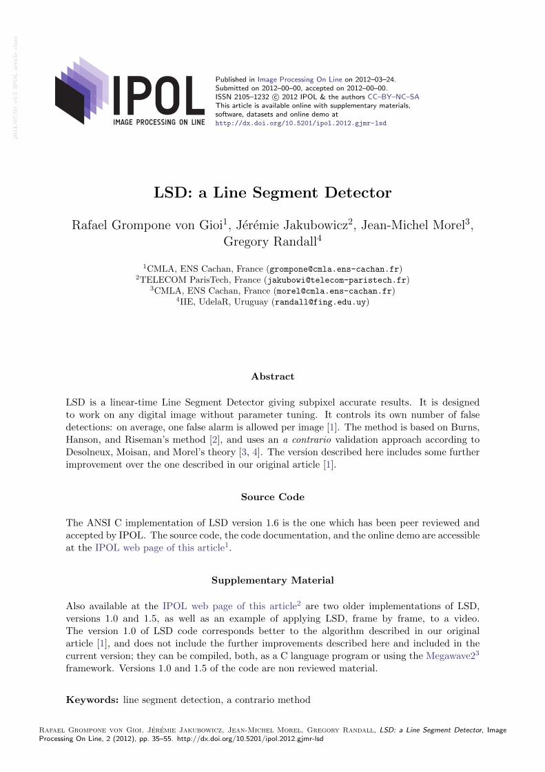
Figure 1: Image gradient and level-lines.

1 Introduction

LSD is aimed at detecting locally straight contours on images. This is what we call line segments.Contours are zones of the image where the gray level is changing fast enough from dark to light orthe opposite. Thus, the gradient and level-lines of the image are key concepts and are illustrated infigure 1.

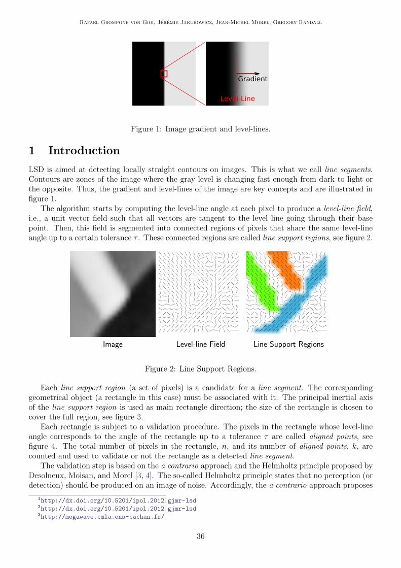
The algorithm starts by computing the level-line angle at each pixel to produce a level-line field,i.e., a unit vector field such that all vectors are tangent to the level line going through their basepoint. Then, this field is segmented into connected regions of pixels that share the same level-lineangle up to a certain tolerance τ . These connected regions are called line support regions, see figure 2.

Image Level-line Field Line Support Regions

Figure 2: Line Support Regions.

Each line support region (a set of pixels) is a candidate for a line segment. The correspondinggeometrical object (a rectangle in this case) must be associated with it. The principal inertial axisof the line support region is used as main rectangle direction; the size of the rectangle is chosen tocover the full region, see figure 3.

Each rectangle is subject to a validation procedure. The pixels in the rectangle whose level-lineangle corresponds to the angle of the rectangle up to a tolerance τ are called aligned points, seefigure 4. The total number of pixels in the rectangle, n, and its number of aligned points, k, arecounted and used to validate or not the rectangle as a detected line segment.

The validation step is based on the a contrario approach and the Helmholtz principle proposed byDesolneux, Moisan, and Morel [3, 4]. The so-called Helmholtz principle states that no perception (ordetection) should be produced on an image of noise. Accordingly, the a contrario approach proposes

1http://dx.doi.org/10.5201/ipol.2012.gjmr-lsd2http://dx.doi.org/10.5201/ipol.2012.gjmr-lsd3http://megawave.cmla.ens-cachan.fr/

36



http://megawave.cmla.ens-cachan.fr/


Figure 3: Rectangle approximation of line support region.

2τ

8 al

igne

d po

ints

Figure 4: Aligned points.

to define a noise or a contrario model H0 where the desired structure is not present. Then, an eventis validated if the expected number of events as good as the observed one is small on the a contrariomodel. In other words, structured events are defined as being rare in the a contrario model.

In the case of line segments, we are interested in the number of aligned points. We consider theevent that a line segment in the a contrario model has as many or more aligned points, as in theobserved line segment. Given an image i and a rectangle r, we will note k(r, i) the number of alignedpoints and n(r) the total number of pixels in r. Then, the expected number of events which are asgood as the observed one is

Ntest · PH0 [k(r, I) ≥ k(r, i)] (1)

where the number of tests Ntest is the total number of possible rectangles being considered, PH0 is theprobability on the a contrario model H0 (that is defined below), and I is a random image followingH0. The H0 stochastic model fixes the distribution of the number of aligned points k(r, I), whichonly depends on the distribution of the level-line field associated with I. Thus H0 is a noise modelfor the image gradient orientation rather than a noise model for the image.

Note that k(r, I) is an abuse of notation as I does not corresponds to an image but to a level-linefield following H0. Nevertheless, there is no contradiction as k(r, I) only depends on the gradientorientations.

The a contrario model H0 used for line segment detection is therefore defined as a stochasticmodel of the level-line field satisfying the following properties:

• {LLA(j)}j∈Pixels is composed of independent random variables

• LLA(j) is uniformly distributed over [0, 2π]

37


where LLA(j) is the level-line angle at pixel j. Under hypothesis H0, the probability that a pixel onthe a contrario model is an aligned point is

p =τ

π

and, as a consequence of the independence of the random variables LLA(j), k(r, I) follows a binomialdistribution. Thus, the probability term PH0 [k(r, I) ≥ k(r, i)] is given by

PH0

[k(r, I) ≥ k(r, i)

]= B

(n(r), k(r, i), p

)where B(n, k, p) is the tail of the binomial distribution:

B(n, k, p) =n∑j=k

(n

j

)pj(1− p)n−j.

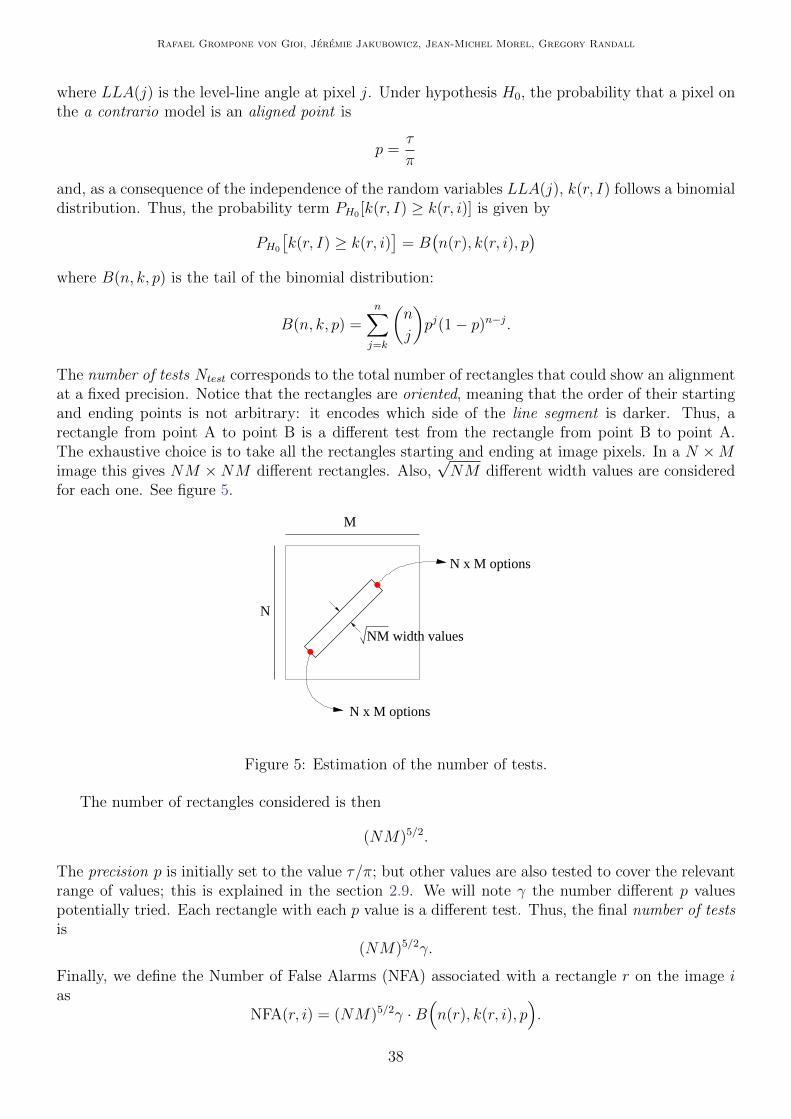
The number of tests Ntest corresponds to the total number of rectangles that could show an alignmentat a fixed precision. Notice that the rectangles are oriented, meaning that the order of their startingand ending points is not arbitrary: it encodes which side of the line segment is darker. Thus, arectangle from point A to point B is a different test from the rectangle from point B to point A.The exhaustive choice is to take all the rectangles starting and ending at image pixels. In a N ×Mimage this gives NM ×NM different rectangles. Also,

√NM different width values are considered

for each one. See figure 5.

NM width values

N x M options

M

N

N x M options

Figure 5: Estimation of the number of tests.

The number of rectangles considered is then

(NM)5/2.

The precision p is initially set to the value τ/π; but other values are also tested to cover the relevantrange of values; this is explained in the section 2.9. We will note γ the number different p valuespotentially tried. Each rectangle with each p value is a different test. Thus, the final number of testsis

(NM)5/2γ.

Finally, we define the Number of False Alarms (NFA) associated with a rectangle r on the image ias

NFA(r, i) = (NM)5/2γ ·B(n(r), k(r, i), p

).

38


This corresponds to the expected number of rectangles which have a sufficient number of alignedpoints to be as rare as r under H0. When the NFA associated with an image rectangle is large, thismeans that such an event is expected on the a contrario model, i.e., common and thus not a relevantone. On the other hand, when the NFA value is small, the event is rare and probably a meaningfulone. A threshold ε is selected and when a rectangle has NFA(r, i) ≤ ε it is called ε-meaningfulrectangle and produces a detection.

Theorem 1

EH0

[∑r∈R

1NFA(r,I)<ε

]≤ ε

where E is the expectation operator, 1 is the indicator function, R is the set of rectangles considered,and I is a random image on H0.

The theorem states that the average number of ε-meaningful rectangles under the a contrariomodel H0 is less than ε. Thus, the number of detections on noise is controlled by ε and it can bemade as small as desired. In other words, this shows that LSD satisfies the Helmholtz principle.

This proof is given here because it was not given in the original article [1].

Proof We define k(r) as

k(r) = min

{κ ∈ N, PH0

[k(r, I) ≥ κ

]≤ ε

(NM)5/2γ

}.

Then, NFA(r, i) ≤ ε is equivalent to k(r, i) ≥ k(r). Now,

EH0

[∑r∈R

1NFA(r,I)≤ε

]=∑r∈R

PH0

[NFA(r, I) ≤ ε

]=∑r∈R

PH0

[k(r, I) ≥ k(r)

].

But, by definition of k(r) we know that

PH0

[k(r, I) ≥ k(r)

]≤ ε

(NM)5/2γ.

and using that #R = (NM)5/2γ we get

EH0

[∑r∈R

1NFA(r,I)≤ε

]≤∑r∈R

ε

(NM)5/2γ= ε

which concludes the proof. �

Following Desolneux, Moisan, and Morel [3, 4], we set ε = 1 once for all. This corresponds toaccepting on average one false detection per image in the a contrario model, which is reasonable.Also, the detection result is not sensitive to the value of ε. Indeed, the detection limit (that is theminimal number of aligned points that could lead to a ε-meaningful rectangle) varies like

√− log ε.

Setting ε to any reasonable value would produce very similar results.

39


Algorithm 1: LSD: Line Segment Detector

input: An image I.output: A list out of rectangles.

1 IS ← ScaleImage(I, S, σ = ΣS

)2 ( LLA, |∇IS|, OrderedListPixels )← Gradient(IS)

3 Status←{

USED, pixels with |∇IS| ≤ ρNOT USED, otherwise

4 foreach pixel P ∈ OrderedListPixels do5 if Status(P ) = NOT USED then6 region← RegionGrow(P, τ)7 rect← Rectangle(region)8 while AlignedPixelDensity(rect, τ) < D do9 region← CutRegion(region)

10 rect← Rectangle(region)

11 end12 rect← ImproveRectangle(rect)13 nfa← NFA(rect)14 if nfa ≤ ε then15 Add rect → out16 end

17 end

18 end

2 Algorithm

The LSD algorithm takes a gray-level image as input and returns a list of detected line segments.Algorithm 1 presents a complete description in pseudocode. The auxiliary image Status has the samesize as the scaled image, and is used to keep track of the pixels already used.

LSD was designed as an automatic image analysis tool. As such it must work without requiringany parameter tuning. The algorithm actually depends on several numbers that determine its be-havior; but their values were carefully devised to work on all images. (See their discussion below.)They are therefore part of LSD’s design, internal parameters, and are not left to the user’s choice.Changing their values would amount to define a new variant of the algorithm, in the same way aswe could make variants by changing the gradient operator, or by switching from 8-neighborhood to4-neighborhood in the region growing process.

Each step of the algorithm will be described in the following sections, as well as the design criteriafor setting the six internal parameters: S, Σ, ρ, τ , D, and ε.

2.1 Image Scaling

The result of LSD is different when the image is analyzed at different scales or if the algorithm isapplied to a small part of the image. This is natural and corresponds to the different details thatone can see if an image is observed from a distance or if attention is paid to a specific part. As aresult of the a contrario validation step, the detection thresholds automatically adapt to the imagesize that is directly related to the number of tests. The scale of analysis is a choice left to the user,who can select it by cropping the image. Otherwise LSD processes automatically the entire image.

The first step of LSD is, nevertheless, to scale the input image to 80% of its size. This scaling

40


helps to cope with aliasing and quantization artifacts (especially the staircase effect) present in manyimages. Blurring the image would produce the same effect but affecting statistics of an image in thea contrario model: some structures would be detected on a blurred white noise. When correctlysub-sampled, the white noise statistics are preserved. Note that the a contrario validation is appliedto the scaled image and the N×M image size used in the NFA computation corresponds to an inputimage of size 1.25N × 1.25M .

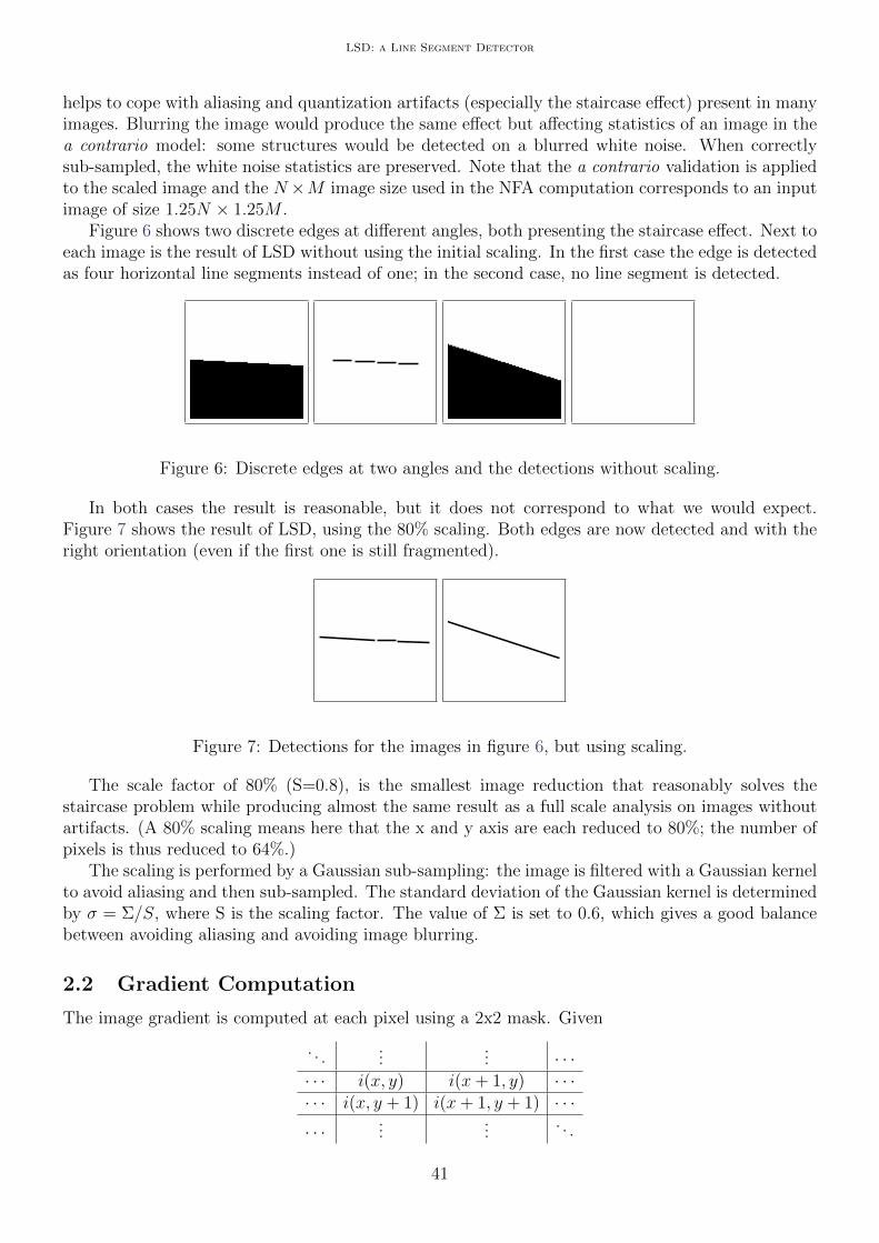
Figure 6 shows two discrete edges at different angles, both presenting the staircase effect. Next toeach image is the result of LSD without using the initial scaling. In the first case the edge is detectedas four horizontal line segments instead of one; in the second case, no line segment is detected.

Figure 6: Discrete edges at two angles and the detections without scaling.

In both cases the result is reasonable, but it does not correspond to what we would expect.Figure 7 shows the result of LSD, using the 80% scaling. Both edges are now detected and with theright orientation (even if the first one is still fragmented).

Figure 7: Detections for the images in figure 6, but using scaling.

The scale factor of 80% (S=0.8), is the smallest image reduction that reasonably solves thestaircase problem while producing almost the same result as a full scale analysis on images withoutartifacts. (A 80% scaling means here that the x and y axis are each reduced to 80%; the number ofpixels is thus reduced to 64%.)

The scaling is performed by a Gaussian sub-sampling: the image is filtered with a Gaussian kernelto avoid aliasing and then sub-sampled. The standard deviation of the Gaussian kernel is determinedby σ = Σ/S, where S is the scaling factor. The value of Σ is set to 0.6, which gives a good balancebetween avoiding aliasing and avoiding image blurring.

2.2 Gradient Computation

The image gradient is computed at each pixel using a 2x2 mask. Given

. . ....

... · · ·· · · i(x, y) i(x+ 1, y) · · ·· · · i(x, y + 1) i(x+ 1, y + 1) · · ·· · · ...

.... . .

41


where i(x, y) is the image gray level value at pixel (x, y), the image gradient is computed as

gx(x, y) =i(x+ 1, y) + i(x+ 1, y + 1)− i(x, y)− i(x, y + 1)

2,

gy(x, y) =i(x, y + 1) + i(x+ 1, y + 1)− i(x, y)− i(x+ 1, y)

2.

The level-line angle is computed as

arctan

(gx(x, y)

−gy(x, y)

)and the gradient magnitude as

G(x, y) =√g2x(x, y) + g2

y(x, y).

This simple scheme uses the smallest possible mask size in its computation, thus reducing as muchas possible the dependence of the computed gradient values (thus, approaching the theoretical inde-pendence in the case of a noise image).

The gradient and level-line angles encode the direction of the edge, that is, the angle of the darkto light transition. Note that a dark to light transition and a light to dark transition are different,having a 180 degree angle difference between the corresponding gradient or level-line angles. Thismeans that the resulting line segments detected by LSD are oriented and that the order of theirstarting and ending points is not arbitrary, since it encodes which side of the line segment is darker.For example, if the contrast of an image is reverted (changing black for white and white for black)the result of LSD would be the same but the starting and ending points would be exchanged onevery line segment.

Note that the computed value corresponds to the image gradient at coordinates (x+ 0.5, y+ 0.5)and not (x, y). This half-pixel offset is then added to the output rectangles coordinates to producecoherent results.

In the a contrario model, the level-line field is composed of independent random variables ateach pixel. But the computed level-line field is actually never fully independent even if the imageis a white noise. Indeed, adjacent pixel values are used to compute the gradient and therefore thegradients are (slightly) dependent. This does not prevent the use of an a contrario approach. Indeed,numerical simulations have shown [5] that the same threshold deduced for the case of independentlevel-line field also controls the number of false detections when computed by the 2x2 mask.

2.3 Gradient Pseudo-Ordering

LSD is a greedy algorithm and the order in which pixels are processed has an impact on the result.Pixels with high gradient magnitude correspond to the more contrasted edges. In an edge, thecentral pixels usually have the highest gradient magnitude. So it makes sense to start looking forline segments at pixels with the highest gradient magnitude.

Sorting algorithms usually require O(n log n) operations to sort n values. However, a simple pixelpseudo-ordering is possible in linear-time. To this aim, 1024 bins are created corresponding to equalgradient magnitude intervals between zero and the largest observed value on the image. Pixels areclassified into the bins according to their gradient magnitude. LSD uses first seed pixels from thebin of the largest gradient magnitudes; then it takes seed pixels from the second bin, and so on untilexhaustion of all bins. 1024 bins are enough to sort almost strictly the gradient values when the graylevel values are quantized in the integer range [0,255].

42


2.4 Gradient Threshold

Pixels with small gradient magnitude correspond to flat zones or slow gradients. Also, they naturallypresent a higher error in the gradient computation due to the quantization of their values. In LSD thepixels with gradient magnitude smaller than ρ are therefore rejected and not used in the constructionof line-support regions or rectangles.

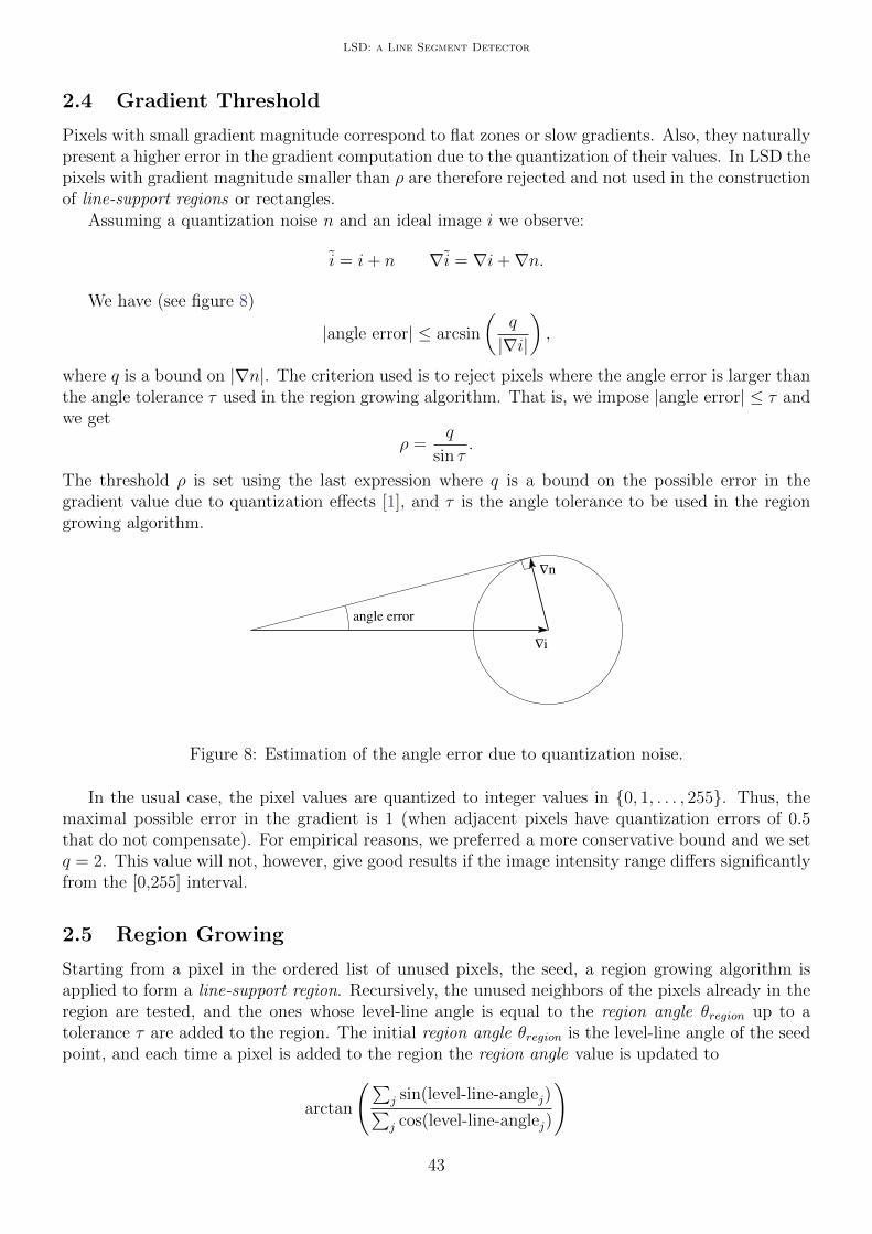
Assuming a quantization noise n and an ideal image i we observe:

i = i+ n ∇i = ∇i+∇n.

We have (see figure 8)

|angle error| ≤ arcsin

(q

|∇i|

),

where q is a bound on |∇n|. The criterion used is to reject pixels where the angle error is larger thanthe angle tolerance τ used in the region growing algorithm. That is, we impose |angle error| ≤ τ andwe get

ρ =q

sin τ.

The threshold ρ is set using the last expression where q is a bound on the possible error in thegradient value due to quantization effects [1], and τ is the angle tolerance to be used in the regiongrowing algorithm.

i

∆

∆

angle error

n

Figure 8: Estimation of the angle error due to quantization noise.

In the usual case, the pixel values are quantized to integer values in {0, 1, . . . , 255}. Thus, themaximal possible error in the gradient is 1 (when adjacent pixels have quantization errors of 0.5that do not compensate). For empirical reasons, we preferred a more conservative bound and we setq = 2. This value will not, however, give good results if the image intensity range differs significantlyfrom the [0,255] interval.

2.5 Region Growing

Starting from a pixel in the ordered list of unused pixels, the seed, a region growing algorithm isapplied to form a line-support region. Recursively, the unused neighbors of the pixels already in theregion are tested, and the ones whose level-line angle is equal to the region angle θregion up to atolerance τ are added to the region. The initial region angle θregion is the level-line angle of the seedpoint, and each time a pixel is added to the region the region angle value is updated to

arctan

(∑j sin(level-line-anglej)∑j cos(level-line-anglej)

)

43


where the index j runs over the pixels in the region. If we associate to each pixel in the regiona unitary vector with its level-line angle, the latter formula corresponds to the angle of the meanvector. The process is repeated until no other pixel can be added to the region. Algorithm 2 gives aprecise definition.

Algorithm 2: RegionGrow

input : A level-line field LLA, a seed pixel P , an angle tolerance τ , and a Status variable foreach pixel.

output: A set of pixels: region.

1 Add P → region2 θregion ← LLA(P )3 Sx ← cos(θregion)4 Sy ← sin(θregion)5 foreach pixel P ∈ region do6 foreach pixel Q ∈ Neighborhood(P ) and Status(Q) 6= USED do7 if AngleDiff

(θregion,LLA(Q)

)< τ then

8 Add Q→ region9 Status(Q)← USED.

10 Sx ← Sx + cos(LLA(Q))11 Sy ← Sy + sin(LLA(Q))12 θregion ← arctan(Sy/Sx).

13 end

14 end

15 end

An 8-connected neighborhood is used, so the neighbors of pixel i(x, y) are i(x−1, y−1), i(x, y−1),i(x+ 1, y − 1), i(x− 1, y), i(x+ 1, y), i(x− 1, y + 1), i(x, y + 1), and i(x+ 1, y + 1).

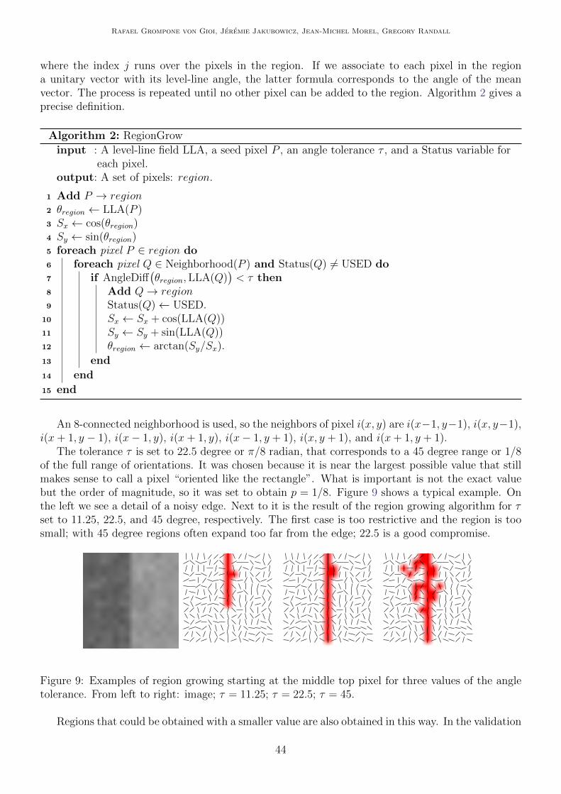
The tolerance τ is set to 22.5 degree or π/8 radian, that corresponds to a 45 degree range or 1/8of the full range of orientations. It was chosen because it is near the largest possible value that stillmakes sense to call a pixel “oriented like the rectangle”. What is important is not the exact valuebut the order of magnitude, so it was set to obtain p = 1/8. Figure 9 shows a typical example. Onthe left we see a detail of a noisy edge. Next to it is the result of the region growing algorithm for τset to 11.25, 22.5, and 45 degree, respectively. The first case is too restrictive and the region is toosmall; with 45 degree regions often expand too far from the edge; 22.5 is a good compromise.

Figure 9: Examples of region growing starting at the middle top pixel for three values of the angletolerance. From left to right: image; τ = 11.25; τ = 22.5; τ = 45.

Regions that could be obtained with a smaller value are also obtained in this way. In the validation

44


process, smaller values of the precision p are also tested, so the value of τ only affects the regiongrowing algorithm and not the validation.

2.6 Rectangular Approximation

A line segment corresponds to a geometrical event, a rectangle. Before evaluating a line-supportregion, the rectangle associated with it must be found. The region of pixels is interpreted as a solidobject and the gradient magnitude of each pixel is used as the “mass” of that point. Then, the centerof mass of the region is selected as the center of the rectangle and the main direction of the rectangleis set to the first inertia axis of the region. Finally, the width and length of the rectangles are set tothe smallest values that make the rectangle to cover the full line-support region.

The center of the rectangle (cx, cy) is set to

cx =

∑j∈RegionG(j) · x(j)∑

j∈Region G(j)

cy =

∑j∈Region G(j) · y(j)∑

j∈RegionG(j)

whereG(j) is the gradient magnitude of pixel j, and the index j runs over the pixels in the region. Themain rectangle’s angle is set to the angle of the eigenvector associated with the smallest eigenvalueof the matrix

M =

(mxx mxy

mxy myy

)with

mxx =

∑j∈Region G(j) · (x(j)− cx)2∑

j∈RegionG(j)

myy =

∑j∈RegionG(j) · (y(j)− cy)2∑

j∈Region G(j)

mxy =

∑j∈RegionG(j) · (x(j)− cx)(y(j)− cy)∑

j∈RegionG(j).

2.7 NFA Computation

A key concept in the validation of a rectangle is that of p-aligned points, namely the pixels in therectangle whose level-line angle is equal to the rectangle’s main orientation, up to a tolerance pπ.The precision p is initially set to the value τ/π, but other values are also tested as is explained in thesection 2.9; a total of γ different values for p are tried. The total number of pixels in the rectangleis denoted by n and the number of p-aligned points is denoted by k (we drop r and i when theyare implicit to simplify the notation). Then, the number of false alarms (NFA) associated with therectangle r is

NFA(r) = (NM)5/2γ ·B(n, k, p)

where N and M are the number of columns and rows of the image (after scaling), and B(n, k, p) isthe binomial tail

B(n, k, p) =n∑j=k

(n

j

)pj(1− p)n−j.

45


All in all, for each rectangle being evaluated and given a precision p, the numbers k and n arecounted, and then the NFA value is computed by

NFA(r) = (NM)5/2γ ·n∑j=k

(n

j

)pj(1− p)n−j.

The rectangles with NFA(r) ≤ ε are validated as detections.As stated before, and following Desolneux, Moisan, and Morel [3, 4], we set ε = 1 once for all. Here

we will only show an experiment illustrating the stability of the result relative to ε value. Figure 10shows the input image and the result of LSD with ε = 1, ε = 10−1, and ε = 10−2, respectively. Onlya few small line segments disappear:

Figure 10: Result of LSD for the image on the left for three different ε values: ε = 1, ε = 10−1, andε = 10−2.

In our implementation, the computation of the binomial tail is performed using the the followingrelation to the Gamma function: (

n

k

)=

Γ(n+ 1)

Γ(k + 1) · Γ(n− k + 1).

The Gamma function can be efficiently computed. We use the methods by Lanczos and Windschitlas described on http://www.rskey.org/gamma.htm. To speed up the computations, the sum of thebinomial tail is truncated when the error can be bounded to be less than 10%.

2.8 Aligned Points Density

In some cases, the τ -angle-tolerance method produces a wrong interpretation. This problem can arisewhen two straight edges are present in the image forming an angle between them smaller than thetolerance τ . Figure 11 shows an example of a line-support region found (in gray) and the rectanglecorresponding to it.

Figure 11: A problem that can arise at the regions growing process.

46

http://www.rskey.org/gamma.htm


This line-support region could be better interpreted as two thinner rectangles, one longer thanthe other, forming an obtuse angle.

In LSD this problem is handled by detecting problematic line-support regions and cutting theminto two smaller regions, hoping to cut the region at the right place to solve the problem. Once acut region is accepted, the rectangle associated is recomputed and the algorithm is resumed.

The detection of this “angle problem” is based on the density of aligned points in the rectangle.When this problem is not present, the rectangle is well adapted to the line-support region and thedensity of aligned points is high. On the other hand, when the “angle problem” is present, as can beseen on the previous figure, the density of aligned points is low. Also, when a slightly curved edgeis being locally approximated by a sequence of straight edges, the degree of the approximation (howmany line segments are used to cover part of curve) is related to the density of aligned points ; thealigned points density is thus also related to the precision at which curves are approximated by linesegments.

The density of aligned points of a rectangle is computed as the ratio of the number of alignedpoints (k in the previous notation) to the area of the rectangle:

d =k

length(r) · width(r).

A threshold D is defined and rectangles should have a density d larger or equal to D to be accepted.We set D to the value 0.7 (70%) which provides good balance between solving the “angle problem”,providing smooth approximations to curves, without over-cutting the line segments.

Two methods for cutting the region are actually tried: reduce angle tolerance and reduce regionradius. In both methods, part of the pixels in the region are kept, while the others are re-markedagain as NOT USED, so they can be used again in future line-support regions. We will describe nowthese two methods:

2.8.1 Reduce Angle Tolerance

The first method, reduce angle tolerance, tries to guess a new tolerance τ ′ that adapts well to theregion, and then the region growing algorithm is used again with the same seed but using the newlyestimated tolerance value. When two straight regions that form an obtuse angle are present, thismethod is expected to get the tolerance that would get only one of these regions, the one containingthe seed pixel.

If all the pixels in the region were used in the estimation of the tolerance, the new value wouldbe such that all the pixels would still be accepted. Instead, only the pixels near the seed are used.Actually, only the pixels whose distance to the seed point is less than the width of the rectangleinitially computed are used. In that way, the size of the neighborhood used in the estimation of τ ′

adapts to the size of the region.All the pixels in that neighborhood of the seed point are evaluated, and the new tolerance τ ′ is

set to twice the standard deviation of the level-line angles of these pixels. With this new value, thesame region growing algorithm is applied, starting from the same seed point. Before that, all thepixels on the original regions are set to NOT USED, so the algorithm can use them again, and thediscarded ones are available for further regions.

2.8.2 Reduce Region Radius

The previous method, reduce angle tolerance, is tried only once, and if the resulting line-supportregion fails to satisfy the density criterion a second method is repetitively tried. The idea of thissecond method is to gradually remove the pixels that are farther from the seed until the criterion

47


is satisfied or the region is too small and rejected. This method works best when the line-supportregion corresponds to a curve and the region needs to be reduced until the density criterion is satisfied,usually meaning that a certain degree of approximation to the curve is obtained.

The distance from the seed point to the farther pixel in the region is called the radius of theregion. Each iteration of this method removes the farthest pixels of the region to reduce the region’sradius to 75% of its value. This process is repeated until the density criterion is satisfied or untilthere are not enough pixels in the region to form a meaningful rectangle. This is just a way ofgradually reducing the region until the criterion is satisfied; it could be done one pixel at a time, butthat would make the process slower.

2.9 Rectangle Improvement

Before rejecting a line-support region for being not meaningful (NFA > ε), LSD tries some variationsof the rectangle’s configuration initially found with the aim to get a valid one.

The relevant factors tested are the precision p used and the width of the rectangle.The initial precision used, corresponding to the region growing tolerance τ is large enough so only

testing smaller values makes sense. If the pixels are well aligned, using a finer precision will keep thesame number of aligned points, but a smaller p yields a smaller (and therefore better) NFA.

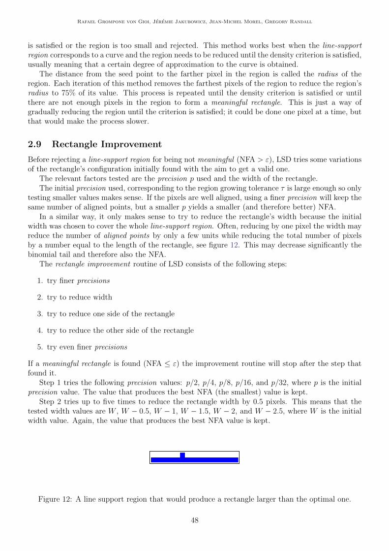
In a similar way, it only makes sense to try to reduce the rectangle’s width because the initialwidth was chosen to cover the whole line-support region. Often, reducing by one pixel the width mayreduce the number of aligned points by only a few units while reducing the total number of pixelsby a number equal to the length of the rectangle, see figure 12. This may decrease significantly thebinomial tail and therefore also the NFA.

The rectangle improvement routine of LSD consists of the following steps:

1. try finer precisions

2. try to reduce width

3. try to reduce one side of the rectangle

4. try to reduce the other side of the rectangle

5. try even finer precisions

If a meaningful rectangle is found (NFA ≤ ε) the improvement routine will stop after the step thatfound it.

Step 1 tries the following precision values: p/2, p/4, p/8, p/16, and p/32, where p is the initialprecision value. The value that produces the best NFA (the smallest) value is kept.

Step 2 tries up to five times to reduce the rectangle width by 0.5 pixels. This means that thetested width values are W , W − 0.5, W − 1, W − 1.5, W − 2, and W − 2.5, where W is the initialwidth value. Again, the value that produces the best NFA value is kept.

Figure 12: A line support region that would produce a rectangle larger than the optimal one.

48


Step 3 tries five times to reduce only one side of the rectangle by 0.5 pixel. This implies reducingthe width of the rectangle by 0.5 pixels but also moving the center of the rectangle by 0.25 pixels tomaintain the position of the other side of the rectangle. So the tested side displacements are 0.5, 1,1.5, 2, and 2.5 pixels. As before, the value that produces the best NFA value is kept.

Step 4 does the same thing as step 3 on the other side of the rectangle.Step 5 tries again to reduce the precision still more. This step tests the precision values p/2, p/4,

p/8, p/16, and p/32, where p is the precision at the beginning of this step. The value that producesthe best NFA value is kept.

In addition to the initial precision p = τπ, five more values are potentially tested in step 1 and

still five more in step 5. Then γ = 11. The range of precisions covered is from p = τπ

to p = τ1024π

and is more than enough to consider any relevant case, the finer precision being about 0.02 degree.Five such steps, attaining a 1 degree precision, would be enough; this refinement, however, worksbetter sometimes before and sometimes after the width refinement, and there is no serious caveat inperforming both.

2.10 Computational Complexity

Performing a Gaussian sub-sampling and computing the image gradient, both can be performed witha number of operations proportional to the number of pixels in the image. Then, pixels are pseudo-ordered by a classification into bins, operation that can be done in linear time. The computationaltime of the line-support region finding algorithm is proportional to the number of visited pixels, andthis number is equal to the total number of pixels in the regions plus the border pixels of each one.Thus, the number of visited pixels remains proportional to the total number of pixels of the image.The rest of the processing can be divided into two kind of tasks. The first kind, for example summingthe region mass or counting aligned points, are proportional to the total number of pixels involvedin all regions. The second kind, like computing inertia moments or computing the NFA value fromthe number of aligned points, are proportional to the number of regions. Both the total number ofpixels involved and the number of regions are at most equal to the number of pixels. All in all, LSDhas an execution time proportional to the number of pixels in the image.

3 Examples

The following set of examples tries to give an idea of the kind of results obtained with LSD, bothgood and bad:

49


Figure 13: Chairs, 512 × 512 pixels. A good result. The detected line segments correspond toempirically straight structures in the image. The detection corresponds roughly with the perceptuallyexpected result.

Figure 14: Molecule LSD, 305× 274 pixels. Note that LSD detects locally straight edges, so eachblack stroke produces two detections, one for each white to black transition. Also note that there isa minimal length that a line segment must have, and smaller ones cannot be detected. (For example,the base of the number ‘2’.) This minimal size for detection depends on the image size because theNFA increases with the image size.

50


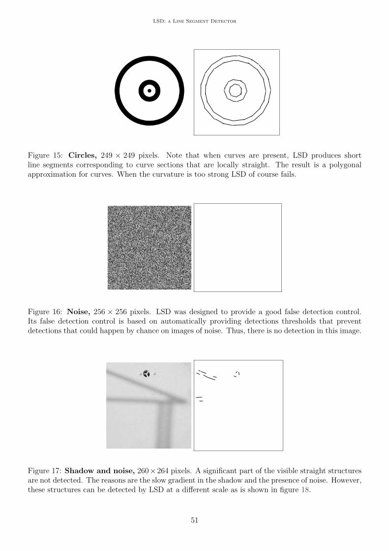
Figure 15: Circles, 249 × 249 pixels. Note that when curves are present, LSD produces shortline segments corresponding to curve sections that are locally straight. The result is a polygonalapproximation for curves. When the curvature is too strong LSD of course fails.

Figure 16: Noise, 256 × 256 pixels. LSD was designed to provide a good false detection control.Its false detection control is based on automatically providing detections thresholds that preventdetections that could happen by chance on images of noise. Thus, there is no detection in this image.

Figure 17: Shadow and noise, 260×264 pixels. A significant part of the visible straight structuresare not detected. The reasons are the slow gradient in the shadow and the presence of noise. However,these structures can be detected by LSD at a different scale as is shown in figure 18.

51


Figure 18: Shadow and noise, subsampling, 130 × 132 pixels. Subsampling of the example infigure 17. When a Gaussian sub-sampling is applied to the previous image, the noise is partiallyremoved and the structure is analyzed at the right scale. The expected line segments are detected.

Figure 19: Small, 417 × 417 pixels. Due to the a contrario framework used by LSD to control thenumber of false detections, the result depends on the image size: the number of tests depends onit. As a consequence, the result of LSD may be locally different if the algorithm is applied to thefull image or to a crop of it. This image contains a little square just under the detection limit. Nodetection is thus produced. However, the next example in figure 20 shows a crop of this same imageand the square is indeed detected. This is the natural behavior of LSD and means that the detaillevel depends on the size of the whole data being analyzed. Human perception is similar: smalldetails often go unnoticed unless attention is drawn to them.

Figure 20: Small, crop, 28× 28 pixels. A crop of the example in figure 19 centered on the square.The square is now detected.

52


Figure 21: Sky, 179× 179 pixels. Some regions are partially anisotropic and partially straight. Suchregions can produce unexpected detections.

Figure 22: Gibbs, 100 × 100 pixels. Image compression, Gibbs effects are responsible for manyunexpected detections.

Figure 23: Color, 254× 254 pixels. LSD is designed to work on gray-level images. Before applyingLSD to a color image it must be converted to a gray-level image. However, some color edges couldbe lost in this conversion. For example, the image on the left presents a clear edge, but after thestandard conversion to a gray-level image (middle) the edge is lost. The reason is that the red valueand the green value are both converted to the same gray value. Thus, LSD will produce no detection(right) because none is present in the input image to LSD (middle). The edge is lost on the colorto gray image conversion and not by LSD. An extension of LSD to deal with this (relatively rare)event is possible but was not done in the current implementation.

53


Figure 24: Piraeus, 600× 600 pixels. Real world scene example. All in all, LSD usually produces areasonable result on real images.

54


Image Credits

All images by the authors.

References

[1] Rafael Grompone von Gioi, Jeremie Jakubowicz, Jean-Michel Morel, Gregory Randall, LSD:A Fast Line Segment Detector with a False Detection Control, IEEE Transactions on PatternAnalysis and Machine Intelligence, vol. 32, no. 4, pp. 722-732, April 2010.http://doi.ieeecomputersociety.org/10.1109/TPAMI.2008.300

[2] J. Brian Burns, Allen R. Hanson, Edward M. Riseman, Extracting Straight Lines, IEEE Trans-actions on Pattern Analysis and Machine Intelligence, vol. 8, no. 4, pp. 425-455, 1986.

[3] Agnes Desolneux, Lionel Moisan, Jean-Michel Morel, Meaningful Alignments, International Jour-nal of Computer Vision, vol. 40, no. 1, pp. 7-23, 2000.http://dx.doi.org/10.1023/A:1026593302236

[4] Agnes Desolneux, Lionel Moisan, Jean-Michel Morel, From Gestalt Theory to Image Analysis, aProbabilistic Approach, Springer 2008. ISBN: 0387726357

[5] Rafael Grompone von Gioi, Jeremie Jakubowicz, Jean-Michel Morel, Gregory Randall, OnStraight Line Segment Detection, Journal of Mathematical Imaging and Vision, vol. 32, no. 3, pp.313-347, November 2008.http://dx.doi.org/10.1007/s10851-008-0102-5

55

http://doi.ieeecomputersociety.org/10.1109/TPAMI.2008.300

http://dx.doi.org/10.1023/A:1026593302236

http://dx.doi.org/10.1007/s10851-008-0102-5

LSD: a Line Segment Detector - IPOL Journal · Image · PDF file ·...

Documents

Transcript of LSD: a Line Segment Detector - IPOL Journal · Image · PDF file ·...