LS-DYNA® Keyword User's Manual (Version 971) - … · ls-dyna® keyword user's manual volume ii...
822
LS-DYNA ® KEYWORD USER'S MANUAL VOLUME II Material Models May 2007 Version 971 LIVERMORE SOFTWARE TECHNOLOGY CORPORATION (LSTC)
Transcript of LS-DYNA® Keyword User's Manual (Version 971) - … · ls-dyna® keyword user's manual volume ii...

LS-DYNA®
KEYWORD USER'S MANUAL
VOLUME II Material Models
May 2007Version 971
LIVERMORE SOFTWARE TECHNOLOGY CORPORATION (LSTC)

Corporate Address Livermore Software Technology Corporation P. O. Box 712 Livermore, California 94551-0712
Support Addresses Livermore Software Technology Corporation 7374 Las Positas Road Livermore, California 94551 Tel: 925-449-2500 Fax: 925-449-2507 Email: [email protected] Website: www.lstc.com
Livermore Software Technology Corporation 1740 West Big Beaver Road Suite 100 Troy, Michigan 48084 Tel: 248-649-4728 Fax: 248-649-6328
Disclaimer Copyright © 1992-2007 Livermore Software Technology Corporation. All Rights Reserved.
LS-DYNA®, LS-OPT® and LS-PrePost® are registered trademarks of Livermore Software Technology Corporation in the United States. All other trademarks, product names and brand names belong to their respective owners.
LSTC reserves the right to modify the material contained within this manual without prior notice.
The information and examples included herein are for illustrative purposes only and are not intended to be exhaustive or all-inclusive. LSTC assumes no liability or responsibility whatsoever for any direct of indirect damages or inaccuracies of any type or nature that could be deemed to have resulted from the use of this manual.
Any reproduction, in whole or in part, of this manual is prohibited without the prior written approval of LSTC. All requests to reproduce the contents hereof should be sent to [email protected].
ISBN 0-9778540-3-5
--------------------------------------------------------------------------------------------------------------------- AES Copyright © 2001, Dr Brian Gladman <[email protected]>, Worcester, UK. All rights reserved.
LICENSE TERMS
The free distribution and use of this software in both source and binary form is allowed (with or without changes) provided that: 1. distributions of this source code include the above copyright notice, this list of conditions and the following
disclaimer; 2. distributions in binary form include the above copyright notice, this list of conditions and the following
disclaimer in the documentation and/or other associated materials; 3. the copyright holder's name is not used to endorse products built using this software without specific written
permission.
DISCLAIMER
This software is provided 'as is' with no explicit or implied warranties in respect of any properties, including, but not limited to, correctness and fitness for purpose. ------------------------------------------------------------------------- Issue Date: 21/01/2002
This file contains the code for implementing the key schedule for AES (Rijndael) for block and key sizes of 16, 24, and 32 bytes.

TABLE OF CONTENTS
LS-DYNA Version 971 iii
TABLE OF CONTENTS
*MAT ...............................................................................................................................................................1
MATERIAL MODEL REFERENCE TABLES ...............................................................................9
*MAT_ADD_EROSION................................................................................................................18
*MAT_ADD_THERMAL_EXPANSION .....................................................................................21
*MAT_NONLOCAL......................................................................................................................22
*MAT_ELASTIC_{OPTION} .......................................................................................................26
*MAT_OPTIONTROPIC_ELASTIC.............................................................................................29
*MAT_PLASTIC_KINEMATIC ...................................................................................................38
*MAT_ELASTIC_PLASTIC_THERMAL....................................................................................41
*MAT_SOIL_AND_FOAM...........................................................................................................44
*MAT_VISCOELASTIC ...............................................................................................................48
*MAT_BLATZ-KO_RUBBER......................................................................................................49
*MAT_HIGH_EXPLOSIVE_BURN.............................................................................................50
*MAT_NULL.................................................................................................................................53
*MAT_ELASTIC_PLASTIC_HYDRO_{OPTION}.....................................................................55
*MAT_STEINBERG......................................................................................................................59
*MAT_STEINBERG_LUND.........................................................................................................64
*MAT_ISOTROPIC_ELASTIC_PLASTIC...................................................................................67
*MAT_ISOTROPIC_ELASTIC_FAILURE..................................................................................68
*MAT_SOIL_AND_FOAM_FAILURE........................................................................................70
*MAT_JOHNSON_COOK ............................................................................................................71
*MAT_PSEUDO_TENSOR...........................................................................................................76
*MAT_ORIENTED_CRACK ........................................................................................................84
*MAT_POWER_LAW_PLASTICITY..........................................................................................86
*MAT_STRAIN_RATE_DEPENDENT_PLASTICITY...............................................................88
*MAT_RIGID ................................................................................................................................91
*MAT_ORTHOTROPIC_THERMAL...........................................................................................96
*MAT_COMPOSITE_DAMAGE................................................................................................101
*MAT_TEMPERATURE_DEPENDENT_ORTHOTROPIC .....................................................105
*MAT_PIECEWISE_LINEAR_PLASTICITY............................................................................110
*MAT_GEOLOGIC_CAP_MODEL ...........................................................................................115
*MAT_HONEYCOMB................................................................................................................121
*MAT_MOONEY-RIVLIN_RUBBER .......................................................................................128
*MAT_RESULTANT_PLASTICITY..........................................................................................131

TABLE OF CONTENTS
iv LS-DYNA Version 971
*MAT_FORCE_LIMITED...........................................................................................................132
*MAT_SHAPE_MEMORY .........................................................................................................138
*MAT_FRAZER_NASH_RUBBER_MODEL............................................................................142
*MAT_LAMINATED_GLASS....................................................................................................145
*MAT_BARLAT_ANISOTROPIC_PLASTICITY.....................................................................147
*MAT_BARLAT_YLD96............................................................................................................151
*MAT_FABRIC ...........................................................................................................................155
*MAT_PLASTIC_GREEN-NAGHDI_RATE .............................................................................163
*MAT_3-PARAMETER_BARLAT.............................................................................................164
*MAT_TRANSVERSELY_ANISOTROPIC_ELASTIC_PLASTIC_{OPTION} ......................171
*MAT_BLATZ-KO_FOAM ........................................................................................................175
*MAT_FLD_TRANSVERSELY_ANISOTROPIC .....................................................................176
*MAT_NONLINEAR_ORTHOTROPIC.....................................................................................178
*MAT_USER_DEFINED_MATERIAL_MODELS....................................................................182
*MAT_BAMMAN .......................................................................................................................186
*MAT_BAMMAN_DAMAGE ....................................................................................................191
*MAT_CLOSED_CELL_FOAM .................................................................................................194
*MAT_ENHANCED_COMPOSITE_DAMAGE ........................................................................197
*MAT_LOW_DENSITY_FOAM ................................................................................................203
*MAT_LAMINATED_COMPOSITE_FABRIC .........................................................................207
*MAT_COMPOSITE_FAILURE_OPTION_MODEL ................................................................213
*MAT_ELASTIC_WITH_VISCOSITY ......................................................................................218
*MAT_ELASTIC_WITH_VISCOSITY_CURVE .......................................................................221
*MAT_KELVIN-MAXWELL_VISCOELASTIC .......................................................................224
*MAT_VISCOUS_FOAM ...........................................................................................................226
*MAT_CRUSHABLE_FOAM.....................................................................................................228
*MAT_RATE_SENSITIVE_POWERLAW_PLASTICITY........................................................230
*MAT_MODIFIED_ZERILLI_ARMSTRONG ..........................................................................232
*MAT_LINEAR_ELASTIC_DISCRETE_BEAM.......................................................................235
*MAT_NONLINEAR_ELASTIC_DISCRETE_BEAM..............................................................237
*MAT_NONLINEAR_PLASTIC_DISCRETE_BEAM ..............................................................240
*MAT_SID_DAMPER_DISCRETE_BEAM ..............................................................................245
*MAT_HYDRAULIC_GAS_DAMPER_DISCRETE_BEAM....................................................249
*MAT_CABLE_DISCRETE_BEAM ..........................................................................................251
*MAT_CONCRETE_DAMAGE .................................................................................................254
*MAT_CONCRETE_DAMAGE_REL3 ......................................................................................258

TABLE OF CONTENTS
LS-DYNA Version 971 v
*MAT_LOW_DENSITY_VISCOUS_FOAM .............................................................................266
*MAT_ELASTIC_SPRING_DISCRETE_BEAM.......................................................................270
*MAT_BILKHU/DUBOIS_FOAM .............................................................................................272
*MAT_GENERAL_VISCOELASTIC.........................................................................................275
*MAT_HYPERELASTIC_RUBBER ..........................................................................................279
*MAT_OGDEN_RUBBER..........................................................................................................283
*MAT_SOIL_CONCRETE..........................................................................................................287
*MAT_HYSTERETIC_SOIL ......................................................................................................291
*MAT_RAMBERG-OSGOOD ....................................................................................................298
*MAT_PLASTICITY_WITH_DAMAGE_{OPTION} ...............................................................300
*MAT_FU_CHANG_FOAM.......................................................................................................308
*MAT_WINFRITH_CONCRETE ...............................................................................................317
*MAT_WINFRITH_CONCRETE_REINFORCEMENT............................................................321
*MAT_ORTHOTROPIC_VISCOELASTIC................................................................................323
*MAT_CELLULAR_RUBBER...................................................................................................326
*MAT_MTS .................................................................................................................................330
*MAT_PLASTICITY_POLYMER..............................................................................................335
*MAT_ACOUSTIC......................................................................................................................338
*MAT_SOFT_TISSUE_{OPTION} ............................................................................................340
*MAT_ELASTIC_6DOF_SPRING_DISCRETE_BEAM...........................................................345
*MAT_INELASTIC_SPRING_DISCRETE_BEAM...................................................................346
*MAT_INELASTIC_6DOF_SPRING_DISCRETE_BEAM.......................................................349
*MAT_BRITTLE_DAMAGE......................................................................................................350
*MAT_GENERAL_JOINT_DISCRETE_BEAM........................................................................353
*MAT_SIMPLIFIED_JOHNSON_COOK ..................................................................................355
*MAT_SIMPLIFIED_JOHNSON_COOK_ORTHOTROPIC_DAMAGE .................................358
*MAT_SPOTWELD_{OPTION} ................................................................................................360
*MAT_SPOTWELD_DAIMLERCHRYSLER............................................................................371
*MAT_GEPLASTIC_SRATE_2000A.........................................................................................374
*MAT_INV_HYPERBOLIC_SIN ...............................................................................................376
*MAT_ANISOTROPIC_VISCOPLASTIC .................................................................................378
*MAT_ANISOTROPIC_PLASTIC .............................................................................................384
*MAT_DAMAGE_1 ....................................................................................................................388
*MAT_DAMAGE_2 ....................................................................................................................394
*MAT_ELASTIC_VISCOPLASTIC_THERMAL ......................................................................398
*MAT_MODIFIED_JOHNSON_COOK.....................................................................................401

TABLE OF CONTENTS
vi LS-DYNA Version 971
*MAT_ORTHO_ELASTIC_PLASTIC........................................................................................410
*MAT_JOHNSON_HOLMQUIST_CERAMICS ........................................................................415
*MAT_JOHNSON_HOLMQUIST_CONCRETE .......................................................................418
*MAT_FINITE_ELASTIC_STRAIN_PLASTICITY..................................................................421
*MAT_TRIP .................................................................................................................................424
*MAT_LAYERED_LINEAR_PLASTICITY..............................................................................428
*MAT_UNIFIED_CREEP............................................................................................................431
*MAT_COMPOSITE_LAYUP ....................................................................................................432
*MAT_COMPOSITE_MATRIX..................................................................................................435
*MAT_COMPOSITE_DIRECT...................................................................................................438
*MAT_GENERAL_NONLINEAR_6DOF_DISCRETE_BEAM................................................440
*MAT_GURSON .........................................................................................................................447
*MAT_GURSON_JC ...................................................................................................................452
*MAT_GURSON_RCDC.............................................................................................................458
*MAT_GENERAL_NONLINEAR_1DOF_DISCRETE_BEAM................................................464
*MAT_HILL_3R ..........................................................................................................................466
*MAT_MODIFIED_PIECEWISE_LINEAR_PLASTICITY_{OPTION} ..................................469
*MAT_PLASTICITY_COMPRESSION_TENSION ..................................................................473
*MAT_KINEMATIC_HARDENING_TRANSVERSELY_ANISOTROPIC.............................476
*MAT_MODIFIED_HONEYCOMB...........................................................................................480
*MAT_ARRUDA_BOYCE_RUBBER........................................................................................489
*MAT_HEART_TISSUE .............................................................................................................492
*MAT_LUNG_TISSUE ...............................................................................................................495
*MAT_SPECIAL_ORTHOTROPIC............................................................................................498
*MAT_ISOTROPIC_SMEARED_CRACK.................................................................................502
*MAT_ORTHOTROPIC_SMEARED_CRACK .........................................................................505
*MAT_BARLAT_YLD2000........................................................................................................510
*MAT_WTM_STM......................................................................................................................516
*MAT_WTM_STM_PLC.............................................................................................................526
*MAT_CORUS_VEGTER...........................................................................................................531
*MAT_COHESIVE_MIXED_MODE..........................................................................................535
*MAT_MODIFIED_FORCE_LIMITED .....................................................................................539
*MAT_VACUUM ........................................................................................................................550
*MAT_RATE_SENSITIVE_POLYMER ....................................................................................551
*MAT_TRANSVERSELY_ISOTROPIC_CRUSHABLE_FOAM .............................................553
*MAT_WOOD_{OPTION} .........................................................................................................557

TABLE OF CONTENTS
LS-DYNA Version 971 vii
*MAT_PITZER_CRUSHABLE_FOAM .....................................................................................564
*MAT_SCHWER_MURRAY_CAP_MODEL............................................................................566
*MAT_1DOF_GENERALIZED_SPRING..................................................................................573
*MAT_FHWA_SOIL ...................................................................................................................575
*MAT_FHWA_SOIL_NEBRASKA............................................................................................578
*MAT_GAS_MIXTURE..............................................................................................................579
*MAT_EMMI...............................................................................................................................585
*MAT_DAMAGE_3 ....................................................................................................................593
*MAT_DESHPANDE_FLECK_FOAM......................................................................................598
*MAT_PLASTICITY_COMPRESSION_TENSION_EOS.........................................................601
*MAT_MUSCLE .........................................................................................................................604
*MAT_ANISOTROPIC_ELASTIC_PLASTIC...........................................................................607
*MAT_RATE_SENSITIVE_COMPOSITE_FABRIC ................................................................610
*MAT_CSCM_{OPTION} ..........................................................................................................615
*MAT_COMPOSITE_MSC_{OPTION}.....................................................................................626
*MAT_MODIFIED_CRUSHABLE_FOAM ...............................................................................637
*MAT_BRAIN_LINEAR_VISCOELASTIC ..............................................................................639
*MAT_PLASTIC_NONLINEAR_KINEMATIC ........................................................................641
*MAT_MOMENT_CURVATURE_BEAM ................................................................................643
*MAT_MCCORMICK.................................................................................................................646
*MAT_POLYMER.......................................................................................................................649
*MAT_ARUP_ADHESIVE .........................................................................................................654
*MAT_RESULTANT_ANISOTROPIC ......................................................................................660
*MAT_STEEL_CONCENTRIC_BRACE ...................................................................................664
*MAT_CONCRETE_EC2............................................................................................................669
*MAT_MOHR_COULOMB........................................................................................................673
*MAT_RC_BEAM.......................................................................................................................678
*MAT_VISCOELASTIC_THERMAL ........................................................................................684
*MAT_QUASILINEAR_VISCOELASTIC.................................................................................688
*MAT_HILL_FOAM ...................................................................................................................693
*MAT_VISCOELASTIC_HILL_FOAM.....................................................................................696
*MAT_LOW_DENSITY_SYNTHETIC_FOAM_{OPTION}....................................................700
*MAT_SIMPLIFIED_RUBBER/FOAM_{OPTION} .................................................................705
*MAT_SIMPLIFIED_RUBBER_WITH_DAMAGE ..................................................................710
*MAT_COHESIVE_ELASTIC....................................................................................................712
*MAT_COHESIVE_TH...............................................................................................................713

TABLE OF CONTENTS
viii LS-DYNA Version 971
*MAT_COHESIVE_GENERAL..................................................................................................716
*MAT_SAMP-1............................................................................................................................720
*MAT_THERMO_ELASTO_VISCOPLASTIC_CREEP............................................................725
*MAT_ANISOTROPIC_THERMOELASTIC.............................................................................729
*MAT_FLD_3-PARAMETER_BARLAT ...................................................................................732
*MAT_SEISMIC_BEAM.............................................................................................................737
*MAT_SOIL_BRICK...................................................................................................................743
*MAT_DRUCKER_PRAGER .....................................................................................................746
*MAT_RC_SHEAR_WALL ........................................................................................................748
*MAT_CONCRETE_BEAM .......................................................................................................755
*MAT_GENERAL_SPRING_DISCRETE_BEAM.....................................................................758
*MAT_SEISMIC_ISOLATOR.....................................................................................................761
*MAT_JOINTED_ROCK ............................................................................................................766
*MAT_ALE_VACUUM ..............................................................................................................770
*MAT_ALE_VISCOUS ...............................................................................................................771
*MAT_ALE_GAS_MIXTURE ....................................................................................................774
*MAT_SPRING_ELASTIC .........................................................................................................780
*MAT_DAMPER_VISCOUS ......................................................................................................781
*MAT_SPRING_ELASTOPLASTIC ..........................................................................................782
*MAT_SPRING_NONLINEAR_ELASTIC ................................................................................783
*MAT_DAMPER_NONLINEAR_VISCOUS .............................................................................784
*MAT_SPRING_GENERAL_NONLINEAR ..............................................................................785
*MAT_SPRING_MAXWELL .....................................................................................................787
*MAT_SPRING_INELASTIC .....................................................................................................789
*MAT_SPRING_TRILINEAR_DEGRADING ...........................................................................790
*MAT_SPRING_SQUAT_SHEARWALL..................................................................................791
*MAT_SPRING_MUSCLE..........................................................................................................792
*MAT_SEATBELT......................................................................................................................797
*MAT_THERMAL_OPTION ......................................................................................................799
*MAT_THERMAL_ISOTROPIC ................................................................................................800
*MAT_THERMAL_ORTHOTROPIC.........................................................................................801
*MAT_THERMAL_ISOTROPIC_TD.........................................................................................803
*MAT_THERMAL_ORTHOTROPIC_TD..................................................................................805
*MAT_THERMAL_ISOTROPIC_PHASE_CHANGE ...............................................................808
*MAT_THERMAL_ISOTROPIC_TD_LC..................................................................................811
*MAT_THERMAL_USER_DEFINED........................................................................................812

*MAT
LS-DYNA Version 971 1 (MAT)
*MAT LS-DYNA has historically referenced each material model by a number. As shown below, a 3-digit numerical designation can still be used, e.g., *MAT_001, and is equivalent to a corresponding descriptive designation, e.g., *MAT_ELASTIC. The two equivalent commands for each material model, one numerical and the other descriptive, are listed below. The numbers in square brackets (see key below) identify the element formulations for which the material model is implemented. The number in the curly brackets, {n}, indicates the default number of history variables per element integration point that are stored in addition to the 7 history variables which are stored by default. For the type 16 fully integrated shell elements with 2 integration points through the thickness, the total number of history variables is 8 x (n+7). For the Belytschko-Tsay type 2 element the number is 2 x (n+7).
An additional option _TITLE may be appended to a *MAT keyword in which case an additional line is read in 80a format which can be used to describe the material. At present, LS-DYNA does not make use of the title. Inclusion of titles simply gives greater clarity to input decks.
Key to numbers in square brackets
0 - Solids 1H - Hughes-Liu beam 1B - Belytschko resultant beam 1I - Belytschko integrated solid and tubular beams 1T - Truss 1D - Discrete beam 1SW - Spotweld beam 2 - Shells 3 - Thick shells 4 - Special airbag element 5 - SPH element 6 - Acoustic solid 7 - Cohesive solid 8A - Multi-material ALE solid (validated) 8B - Multi-material ALE solid (implemented but not validated1)
*MAT_ADD_EROSION 2
*MAT_ADD_THERMAL_EXPANSION 2
*MAT_NONLOCAL 2
*MAT_001: *MAT_ELASTIC [0,1H,1B,1I,1T,2,3,5,8A] {0}
*MAT_001_FLUID: *MAT_ELASTIC_FLUID [0,8A] {0}
1 Error associated with advection inherently leads to state variables that may be inconsistent with nonlinear constitutive routines and thus may lead to nonphysical results, nonconservation of energy, and even numerical instability in some cases. Caution is advised, particularly when using the 2nd tier of material models implemented for ALE multi-material solids (designated by [8B]) which are largely untested as ALE materials. 2 These three commands do not, by themselves, define a material model but rather can be used in certain cases to supplement material models.

*MAT
2 (MAT) LS-DYNA Version 971
*MAT_002: *MAT_OPTIONTROPIC_ELASTIC [0,2,3] {15}
*MAT_003: *MAT_PLASTIC_KINEMATIC [0,1H,1I,1T,2,3,5,8A] {5}
*MAT_004: *MAT_ELASTIC_PLASTIC_THERMAL [0,1H,1T,2,3,8B] {3}
*MAT_005: *MAT_SOIL_AND_FOAM [0,5,8A] {0}
*MAT_006: *MAT_VISCOELASTIC [0,1H,2,5,8B] {19}
*MAT_007: *MAT_BLATZ-KO_RUBBER [0,2,8B] {9}
*MAT_008: *MAT_HIGH_EXPLOSIVE_BURN [0,5,8A] {4}
*MAT_009: *MAT_NULL [0,1,2,5,8A] {3}
*MAT_010: *MAT_ELASTIC_PLASTIC_HYDRO_{OPTION} [0,5,8B] {4}
*MAT_011: *MAT_STEINBERG [0,5,8B] {5}
*MAT_011_LUND: *MAT_STEINBERG_LUND [0,5,8B] {5}
*MAT_012: *MAT_ISOTROPIC_ELASTIC_PLASTIC [0,2,3,5,8B] {0}
*MAT_013: *MAT_ISOTROPIC_ELASTIC_FAILURE [0,5,8B] {1}
*MAT_014: *MAT_SOIL_AND_FOAM_FAILURE [0,5,8B] {1}
*MAT_015: *MAT_JOHNSON_COOK [0,2,3,5,8A] {6}
*MAT_016: *MAT_PSEUDO_TENSOR [0,5,8B] {6}
*MAT_017: *MAT_ORIENTED_CRACK [0] {10}
*MAT_018: *MAT_POWER_LAW_PLASTICITY [0,1H,2,3,5,8B] {0}
*MAT_019: *MAT_STRAIN_RATE_DEPENDENT_PLASTICITY [0,2,3,5,8B] {6}
*MAT_020: *MAT_RIGID [0,1H,1B,1T,2,3] {0}
*MAT_021: *MAT_ORTHOTROPIC_THERMAL [0,2,3] {29}
*MAT_022: *MAT_COMPOSITE_DAMAGE [0,2,3] {12}
*MAT_023: *MAT_TEMPERATURE_DEPENDENT_ORTHOTROPIC [0,2,3] {19}
*MAT_024: *MAT_PIECEWISE_LINEAR_PLASTICITY [0,1H,2,3,5,8A] {5}
*MAT_025: *MAT_GEOLOGIC_CAP_MODEL [0,5] {12}
*MAT_026: *MAT_HONEYCOMB [0] {20}
*MAT_027: *MAT_MOONEY-RIVLIN_RUBBER [0,1T,2,8B] {9}
*MAT_028: *MAT_RESULTANT_PLASTICITY [1B,2] {5}
*MAT_029: *MAT_FORCE_LIMITED [1B] {30}
*MAT_030: *MAT_SHAPE_MEMORY [0,2,5] {23}
*MAT_031: *MAT_FRAZER_NASH_RUBBER_MODEL [0,8B] {9}
*MAT_032: *MAT_LAMINATED_GLASS [2,3] {0}
*MAT_033: *MAT_BARLAT_ANISOTROPIC_PLASTICITY [0,2,3] {9}
*MAT_033_96: *MAT_BARLAT_YLD96 [2,3] {9}
*MAT_034: *MAT_FABRIC [4] {17}
*MAT_035: *MAT_PLASTIC_GREEN-NAGHDI_RATE [0,5,8B] {22}
*MAT_036: *MAT_3-PARAMETER_BARLAT [2,3] {7}

*MAT
LS-DYNA Version 971 3 (MAT)
*MAT_037: *MAT_TRANSVERSELY_ANISOTROPIC_ELASTIC_PLASTIC [2,3] {9}
*MAT_038: *MAT_BLATZ-KO_FOAM [0,2,8B] {9}
*MAT_039: *MAT_FLD_TRANSVERSELY_ANISOTROPIC [2,3] {6}
*MAT_040: *MAT_NONLINEAR_ORTHOTROPIC [0,2] {17}
*MAT_041-050: *MAT_USER_DEFINED_MATERIAL_MODELS [0,1H,1T,1D,2,3,5,8B] {0}
*MAT_051: *MAT_BAMMAN [0,2,3,5,8B] {8}
*MAT_052: *MAT_BAMMAN_DAMAGE [0,2,3,5,8B] {10}
*MAT_053: *MAT_CLOSED_CELL_FOAM [0,8B] {0}
*MAT_054-055: *MAT_ENHANCED_COMPOSITE_DAMAGE [2] {20}
*MAT_057: *MAT_LOW_DENSITY_FOAM [0,5,8B] {26}
*MAT_058: *MAT_LAMINATED_COMPOSITE_FABRIC [2,3] {15}
*MAT_059: *MAT_COMPOSITE_FAILURE_OPTION_MODEL [0,2] {22}
*MAT_060: *MAT_ELASTIC_WITH_VISCOSITY [0,2,5,8B] {8}
*MAT_060C: *MAT_ELASTIC_WITH_VISCOSITY_CURVE [0,2,5,8B] {8}
*MAT_061: *MAT_KELVIN-MAXWELL_VISCOELASTIC [0,5,8B] {14}
*MAT_062: *MAT_VISCOUS_FOAM [0,8B] {7}
*MAT_063: *MAT_CRUSHABLE_FOAM [0,5,8B] {8}
*MAT_064: *MAT_RATE_SENSITIVE_POWERLAW_PLASTICITY [0,2,3,5,8B] {30}
*MAT_065: *MAT_MODIFIED_ZERILLI_ARMSTRONG [0,2,3,5,8B] {6}
*MAT_066: *MAT_LINEAR_ELASITC_DISCRETE_BEAM [1D] {8}
*MAT_067: *MAT_NONLINEAR_ELASITC_DISCRETE_BEAM [1D] {14}
*MAT_068: *MAT_NONLINEAR_PLASITC_DISCRETE_BEAM [1D] {25}
*MAT_069: *MAT_SID_DAMPER_DISCRETE_BEAM [1D] {13}
*MAT_070: *MAT_HYDRAULIC_GAS_DAMPER_DISCRETE_BEAM [1D] {8}
*MAT_071: *MAT_CABLE_DISCRETE_BEAM [1D] {8}
*MAT_072: *MAT_CONCRETE_DAMAGE [0,5,8B] {6}
*MAT_072R3: *MAT_CONCRETE_DAMAGE_REL3 [0,5] {6}
*MAT_073: *MAT_LOW_DENSITY_VISCOUS_FOAM [0,8B] {56}
*MAT_074: *MAT_ELASTIC_SPRING_DISCRETE_BEAM [1D] {8}
*MAT_075: *MAT_BILKHU/DUBOIS_FOAM [0,5,8B] {8}
*MAT_076: *MAT_GENERAL_VISCOELASTIC [0,2,5,8B] {53}
*MAT_077_H: *MAT_HYPERELASTIC_RUBBER [0,2,5,8B] {54}
*MAT_077_O: *MAT_OGDEN_RUBBER [0,2,8B] {54}
*MAT_078: *MAT_SOIL_CONCRETE [0,8B] {3}
*MAT_079: *MAT_HYSTERETIC_SOIL [0,5,8B] {77}
*MAT_080: *MAT_RAMBERG-OSGOOD [0,8B] {18}
*MAT_081: *MAT_PLASTICITY_WITH_DAMAGE [0,2,3] {5}

*MAT
4 (MAT) LS-DYNA Version 971
*MAT_082(_RCDC): *MAT_PLASTICITY_WITH_DAMAGE_ORTHO(_RCDC) [0,2,3] {22}
*MAT_083: *MAT_FU_CHANG_FOAM [0,5,8B] {54}
*MAT_084-085: *MAT_WINFRITH_CONCRETE [0,8B] {54}
*MAT_086: *MAT_ORTHOTROPIC_VISCOELASTIC [2,3] {17}
*MAT_087: *MAT_CELLULAR_RUBBER [0,5,8B] {19}
*MAT_088: *MAT_MTS [0,2,3,5,8B] {5}
*MAT_089: *MAT_PLASTICITY_POLYMER [2] {45}
*MAT_090: *MAT_ACOUSTIC [6] {25}
*MAT_091: *MAT_SOFT_TISSUE [0,2] {16}
*MAT_092: *MAT_SOFT_TISSUE_VISCO [0,2] {58}
*MAT_093: *MAT_ELASTIC_6DOF_SPRING_DISCRETE_BEAM [1D] {25}
*MAT_094: *MAT_INELASTIC_SPRING_DISCRETE_BEAM [1D] {9}
*MAT_095: *MAT_INELASTC_6DOF_SPRING_DISCRETE_BEAM [1D] {25}
*MAT_096: *MAT_BRITTLE_DAMAGE [0,8B] {51}
*MAT_097: *MAT_GENERAL_JOINT_DISCRETE_BEAM [1D] {23}
*MAT_098: *MAT_SIMPLIFIED_JOHNSON_COOK [0,1H,1B,1T,2,3] {6}
*MAT_099: *MAT_SIMPLIFIED_JOHNSON_COOK_ORTHOTROPIC_DAMAGE [0,2,3] {22}
*MAT_100: *MAT_SPOTWELD_{OPTION} [0,1SW] {6}
*MAT_100_DA: *MAT_SPOTWELD_DAIMLERCHRYSLER [0] {6}
*MAT_101: *MAT_GEPLASTIC_SRATE_2000A [2] {15}
*MAT_102: *MAT_INV_HYPERBOLIC_SIN [0,8B] {15}
*MAT_103: *MAT_ANISOTROPIC_VISCOPLASTIC [0,2,3,5] {20}
*MAT_103_P: *MAT_ANISOTROPIC_PLASTIC [2,3] {20}
*MAT_104: *MAT_DAMAGE_1 [0,2,3] {11}
*MAT_105: *MAT_DAMAGE_2 [0,2,3] {7}
*MAT_106: *MAT_ELASTIC_VISCOPLASTIC_THERMAL [0,2] {20}
*MAT_107: *MAT_MODIFIED_JOHNSON_COOK [0,2,5,8B] {15}
*MAT_108: *MAT_ORTHO_ELASTIC_PLASTIC [2] {15}
*MAT_110: *MAT_JOHNSON_HOLMQUIST_CERAMICS [0,5] {15}
*MAT_111: *MAT_JOHNSON_HOLMQUIST_CONCRETE [0,5] {25}
*MAT_112: *MAT_FINITE_ELASTIC_STRAIN_PLASTICITY [0,5] {22}
*MAT_113: *MAT_TRIP [2] {5}
*MAT_114: *MAT_LAYERED_LINEAR_PLASTICITY [2] {13}
*MAT_115: *MAT_UNIFIED_CREEP [0,2,5] {1}
*MAT_116: *MAT_COMPOSITE_LAYUP [2] {30}
*MAT_117: *MAT_COMPOSITE_MATRIX [2] {30}
*MAT_118: *MAT_COMPOSITE_DIRECT [2] {10}

*MAT
LS-DYNA Version 971 5 (MAT)
*MAT_119: *MAT_GENERAL_NONLINEAR_6DOF_DISCRETE_BEAM [1D] {62}
*MAT_120: *MAT_GURSON [0,2] {12}
*MAT_120_JC: *MAT_GURSON_JC [0,2] {12}
*MAT_120_RCDC: *MAT_GURSON_RCDC [0,2] {12}
*MAT_121: *MAT_GENERAL_NONLINEAR_1DOF_DISCRETE_BEAM [1D] {20}
*MAT_122: *MAT_HILL_3R [2,3] {8}
*MAT_123: *MAT_MODIFIED_PIECEWISE_LINEAR_PLASTICITY [0,2,3] {11}
*MAT_124: *MAT_PLASTICITY_COMPRESSION_TENSION [0,2,3,5,8B] {7}
*MAT_125: *MAT_KINEMATIC_HARDENING_TRANSVERSELY_ANISOTROPIC [2] {11}
*MAT_126: *MAT_MODIFIED_HONEYCOMB [0] {20}
*MAT_127: *MAT_ARRUDA_BOYCE_RUBBER [0,5] {49}
*MAT_128: *MAT_HEART_TISSUE [0] {15}
*MAT_129: *MAT_LUNG_TISSUE [0] {49}
*MAT_130: *MAT_SPECIAL_ORTHOTROPIC [2] {35}
*MAT_131: *MAT_ISOTROPIC_SMEARED_CRACK [0,5,8B] {15}
*MAT_132: *MAT_ORTHOTROPIC_SMEARED_CRACK [0] {61}
*MAT_133: *MAT_BARLAT_YLD2000 [2,3] {9}
*MAT_135: *MAT_WTM_STM [2,3] {30}
*MAT_135_PLC: *MAT_WTM_STM_PLC [2,3] {30}
*MAT_136: *MAT_CORUS_VEGTER [2] {5}
*MAT_138: *MAT_COHESIVE_MIXED_MODE [7] {0}
*MAT_139: *MAT_MODIFIED_FORCE_LIMITED [1B] {35}
*MAT_140: *MAT_VACUUM [0,8A] {0}
*MAT_141: *MAT_RATE_SENSITIVE_POLYMER [0,8B] {6}
*MAT_142: *MAT_TRANSVERSELY_ANISOTROPIC_CRUSHABLE_FOAM [0] {12}
*MAT_143: *MAT_WOOD_{OPTION} [0] {37}
*MAT_144: *MAT_PITZER_CRUSHABLE FOAM [0,8B] {7}
*MAT_145: *MAT_SCHWER_MURRAY_CAP_MODEL [0,5] {50}
*MAT_146: *MAT_1DOF_GENERALIZED_SPRING [1D] {1}
*MAT_147 *MAT_FHWA_SOIL [0,5,8B] {15}
*MAT_147_N: *MAT_FHWA_SOIL_NEBRASKA [0,5,8B] {15}
*MAT_148: *MAT_GAS_MIXTURE [0,8A] {14}
*MAT_151: *MAT_EMMI [0,5,8B] {23}
*MAT_153: *MAT_DAMAGE_3 [0,1H,2,3]
*MAT_154: *MAT_DESHPANDE_FLECK_FOAM [0,8B] {10}
*MAT_155: *MAT_PLASTICITY_COMPRESSION_TENSION_EOS [0,5,8B] {16}
*MAT_156: *MAT_MUSCLE [1T] {0}

*MAT
6 (MAT) LS-DYNA Version 971
*MAT_157: *MAT_ANISOTROPIC_ELASTIC_PLASTIC [2] {5}
*MAT_158: *MAT_RATE_SENSITIVE_COMPOSITE_FABRIC [2,3] {54}
*MAT_159: *MAT_CSCM_{OPTION} [0] {22}
*MAT_161: *MAT_COMPOSITE_MSC [0] {34}
*MAT_162: *MAT_COMPOSITE_DMG_MSC [0,2] {40}
*MAT_163 *MAT_MODIFIED_CRUSHABLE_FOAM [0,8B] {10}
*MAT_164: *MAT_BRAIN_LINEAR_VISCOELASTIC [0] {14}
*MAT_165: *MAT_PLASTIC_NONLINEAR_KINEMATIC [0,2,8B] {8}
*MAT_166: *MAT_MOMENT_CURVATURE_BEAM [1B] {54}
*MAT_167: *MAT_MCCORMICK [0,8B] {8}
*MAT_168: *MAT_POLYMER [0,8B] {60}
*MAT_169: *MAT_ARUP_ADHESIVE [0] {20}
*MAT_170: *MAT_RESULTANT_ANISOTROPIC [2] {67}
*MAT_171: *MAT_STEEL_CONCENTRIC_BRACE [1B] {33}
*MAT_172: *MAT_CONCRETE_EC2 [1H,2] {35}
*MAT_173: *MAT_MOHR_COULOMB [0] {31}
*MAT_174: *MAT_RC_BEAM [1H] {26}
*MAT_175: *MAT_VISCOELASTIC_THERMAL [0,2,5,8B] {86}
*MAT_176: *MAT_QUASILINEAR_VISCOELASTIC [0,2,5,8B] {81}
*MAT_177: *MAT_HILL_FOAM [0] {12}
*MAT_178: *MAT_VISCOELASTIC_HILL_FOAM [0] {92}
*MAT_179: *MAT_LOW_DENSITY_SYNTHETIC_FOAM_{OPTION} [0] {77}
*MAT_181: *MAT_SIMPLIFIED_RUBBER/FOAM_{OPTION} [0,2] {39}
*MAT_183: *MAT_SIMPLIFIED_RUBBER_WITH_DAMAGE [0,2] {44}
*MAT_184: *MAT_COHESIVE_ELASTIC [7] {0}
*MAT_185: *MAT_COHESIVE_TH [7] {0}
*MAT_186: *MAT_COHESIVE GENERAL [7] {6}
*MAT_187: *MAT_SAMP-1 [0,2] {38}
*MAT_188: *MAT_THERMO_ELASTO_VISCOPLASTIC_CREEP [0,2] {27}
*MAT_189: *MAT_ANISOTROPIC_THERMOELASTIC [0,8B] {21}
*MAT_190: *MAT_FLD_3-PARAMETER_BARLAT [2] {36}
*MAT_191: *MAT_SEISMIC_BEAM [1B] {36}
*MAT_192: *MAT_SOIL_BRICK [0] {71}
*MAT_193: *MAT_DRUCKER_PRAGER [0] {74}
*MAT_194: *MAT_RC_SHEAR_WALL [2] {36}
*MAT_195: *MAT_CONCRETE_BEAM [1H] {5}
*MAT_196: *MAT_GENERAL_SPRING_DISCRETE_BEAM [1D] {25}

*MAT
LS-DYNA Version 971 7 (MAT)
*MAT_197: *MAT_SEISMIC_ISOLATOR [1D] {10}
*MAT_198: *MAT_JOINTED_ROCK [0] {31}
For the discrete (type 6) beam elements, which are used to model complicated dampers and multi-dimensional spring-damper combinations, the following material types are available:
*MAT_066: *MAT_LINEAR_ELASTIC_DISCRETE_BEAM [1D]
*MAT_067: *MAT_NONLINEAR_ELASTIC_DISCRETE_BEAM [1D]
*MAT_068: *MAT_NONLINEAR_PLASTIC_DISCRETE_BEAM [1D]
*MAT_069: *MAT_SID_DAMPER_DISCRETE_BEAM [1D]
*MAT_070: *MAT_HYDRAULIC_GAS_DAMPER_DISCRETE_BEAM [1D]
*MAT_071: *MAT_CABLE_DISCRETE_BEAM [1D]
*MAT_074: *MAT_ELASTIC_SPRING_DISCRETE_BEAM [1D]
*MAT_093: *MAT_ELASTIC_6DOF_SPRING_DISCRETE_BEAM [1D]
*MAT_094: *MAT_INELASTIC_SPRING_DISCRETE_BEAM [1D]
*MAT_095: *MAT_INELASTIC_6DOF_SPRING_DISCRETE_BEAM [1D]
*MAT_119: *MAT_GENERAL_NONLINEAR_6DOF_DISCRETE_BEAM [1D]
*MAT_121: *MAT_GENERAL_NONLINEAR_1DOF_DISCRETE_BEAM [1D]
*MAT_146: *MAT_1DOF_GENERALIZED_SPRING [1D]
*MAT_196: *MAT_GENERAL_SPRING_DISCRETE_BEAM [1D]
*MAT_197: *MAT_SEISMIC_ISOLATOR [1D]
For the discrete springs and dampers the following material types are available.
*MAT_S01: *MAT_SPRING_ELASTIC
*MAT_S02: *MAT_DAMPER_VISCOUS
*MAT_S03: *MAT_SPRING_ELASTOPLASTIC
*MAT_S04: *MAT_SPRING_NONLINEAR_ELASTIC
*MAT_S05: *MAT_DAMPER_NONLINEAR_VISCOUS
*MAT_S06: *MAT_SPRING_GENERAL_NONLINEAR
*MAT_S07: *MAT_SPRING_MAXWELL
*MAT_S08: *MAT_SPRING_INELASTIC
*MAT_S13: *MAT_SPRING_TRILINEAR_DEGRADING
*MAT_S14: *MAT_SPRING_SQUAT_SHEARWALL
*MAT_S15: *MAT_SPRING_MUSCLE

*MAT
8 (MAT) LS-DYNA Version 971
For ALE solids the following material types are available:
*MAT_ALE_01: *MAT_ALE_VACUUM (same as *MAT_140)
*MAT_ALE_02: *MAT_ALE_VISCOUS (similar to *MAT_009)
*MAT_ALE_03: *MAT_ALE_GAS_MIXTURE (same as *MAT_148)
For the seatbelts one material is available.
*MAT_B01: *MAT_SEATBELT
For thermal materials in a coupled structural/thermal or thermal only analysis, six materials are available. These materials are related to the structural material via the *PART card. Thermal materials are defined only for solid and shell elements.
*MAT_THERMAL_OPTION
*MAT_T01: *MAT_THERMAL_ISOTROPIC
*MAT_T02: *MAT_THERMAL_ORTHOTROPIC
*MAT_T03: *MAT_THERMAL_ISOTROPIC_TD
*MAT_T04: *MAT_THERMAL_ORTHOTROPIC_TD
*MAT_T05: *MAT_THERMAL_ISOTROPIC_PHASE_CHANGE
*MAT_T06: *MAT_THERMAL_ISOTROPIC_TD_LC
*MAT_T11-T15: *MAT_THERMAL_USER_DEFINED

MATERIAL MODEL REFERENCE TABLES *MAT
LS-DYNA Version 971 9 (MAT)
MATERIAL MODEL REFERENCE TABLES
The tables provided on the following pages list the material models, some of their attributes, and the general classes of physical materials to which the numerical models might be applied.
If a material model includes any of the following attributes, a “Y” will appear in the respective column of the table:
SRATE - Strain-rate effects
FAIL - Failure criteria
EOS - Equation-of-State required for 3D solids and 2D continuum elements
THERM - Thermal effects
ANISO - Anisotropic/orthotropic
DAM - Damage effects
TENS - Tension handled differently than compression in some manner
Potential applications of the material models, in terms of classes of physical materials, are abbreviated in the table as follows:
GN - General
CM - Composite
CR - Ceramic
FL - Fluid
FM - Foam
GL - Glass
HY - Hydrodynamic material
MT - Metal
PL - Plastic
RB - Rubber
SL - Soil, concrete, or rock
AD - Adhesive
BIO - Biological material
CIV - Civil Engineering component

*MAT MATERIAL MODEL REFERENCE TABLES
10 (MAT) LS-DYNA Version 971
Material Number and Description SRA
TE
FA
IL
EO
S
TH
ER
M
AN
ISO
DA
M
TE
NS
Applications
1 Elastic GN, FL
2 Orthotropic Elastic (Anisotropic-solids) Y CM, MT
3 Plastic Kinematic/Isotropic Y Y CM, MT, PL
4 Elastic Plastic Thermal Y MT, PL
5 Soil and Foam Y FM, SL
6 Linear Viscoelastic Y RB
7 Blatz-Ko Rubber RB
8 High Explosive Burn Y HY
9 Null Material Y Y Y Y FL, HY
10 Elastic Plastic Hydro(dynamic) Y Y Y HY, MT
11 Steinberg: Temp. Dependent Elastoplastic Y Y Y Y Y HY, MT
12 Isotropic Elastic Plastic MT
13 Isotropic Elastic Plastic with Failure Y Y MT
14 Soil and Foam with Failure Y Y FM, SL
15 Johnson/Cook Plasticity Model Y Y Y Y Y Y HY, MT
16 Pseudo Tensor Geological Model Y Y Y Y Y SL
17 Oriented Crack (Elastoplastic w/ Fracture) Y Y Y Y HY, MT, PL, CR
18 Power Law Plasticity (Isotropic) Y MT, PL
19 Strain Rate Dependent Plasticity Y Y MT, PL
20 Rigid
21 Orthotropic Thermal (Elastic) Y Y GN
22 Composite Damage Y Y Y CM
23 Temperature Dependent Orthotropic Y Y CM
24 Piecewise Linear Plasticity (Isotropic) Y Y MT, PL
25 Inviscid Two Invariant Geologic Cap Y Y SL
26 Honeycomb Y Y Y Y CM, FM, SL
27 Mooney-Rivlin Rubber Y RB

MATERIAL MODEL REFERENCE TABLES *MAT
LS-DYNA Version 971 11 (MAT)
Material Number and Description SRA
TE
FA
IL
EO
S
TH
ER
M
AN
ISO
DA
M
TE
NS
Applications
28 Resultant Plasticity MT
29 Force Limited Resultant Formulation Y
30 Shape Memory MT
31 Frazer-Nash Rubber Y RB
32 Laminated Glass (Composite) Y CM, GL
33 Barlat Anisotropic Plasticity (YLD96) Y Y CR, MT
34 Fabric Y Y fabric
35 Plastic-Green Naghdi Rate Y MT
36 Three-Parameter Barlat Plasticity Y Y MT
37 Transversely Anisotropic Elastic Plastic Y MT
38 Blatz-Ko Foam FM, PL
39 FLD Transversely Anisotropic Y MT
40 Nonlinear Orthotropic Y Y Y Y CM
41-50 User Defined Materials Y Y Y Y Y Y Y GN
51 Bamman (Temp/Rate Dependent Plasticity) Y Y GN
52 Bamman Damage Y Y Y Y MT
53 Closed cell foam (Low density polyurethane) FM
54 Composite Damage with Chang Failure Y Y Y Y CM
55 Composite Damage with Tsai-Wu Failure Y Y Y Y CM
57 Low Density Urethane Foam Y Y Y FM
58 Laminated Composite Fabric Y Y Y Y CM, fabric
59 Composite Failure (Plasticity Based) Y Y Y CM, CR
60 Elastic with Viscosity (Viscous Glass) Y Y GL
61 Kelvin-Maxwell Viscoelastic Y FM
62 Viscous Foam (Crash dummy Foam) Y FM
63 Isotropic Crushable Foam Y FM
64 Rate Sensitive Powerlaw Plasticity Y MT

*MAT MATERIAL MODEL REFERENCE TABLES
12 (MAT) LS-DYNA Version 971
Material Number and Description SRA
TE
FA
IL
EO
S
TH
ER
M
AN
ISO
DA
M
TE
NS
Applications
65 Zerilli-Armstrong (Rate/Temp Plasticity) Y Y Y Y MT
66 Linear Elastic Discrete Beam Y Y
67 Nonlinear Elastic Discrete Beam Y Y Y
68 Nonlinear Plastic Discrete Beam Y Y Y
69 SID Damper Discrete Beam Y
70 Hydraulic Gas Damper Discrete Beam Y
71 Cable Discrete Beam (Elastic) Y cable
72 Concrete Damage (incl. Release III) Y Y Y Y Y SL
73 Low Density Viscous Foam Y Y Y FM
74 Elastic Spring Discrete Beam Y Y Y
75 Bilkhu/Dubois Foam Y FM
76 General Viscoelastic (Maxwell Model) Y Y Y RB
77 Hyperelastic and Ogden Rubber Y Y RB
78 Soil Concrete Y Y Y SL
79 Hysteretic Soil (Elasto-Perfectly Plastic) Y Y SL
80 Ramberg-Osgood SL
81 Plasticity with Damage Y Y Y MT, PL
82 Plasticity with Damage Ortho Y Y Y Y
83 Fu Chang Foam Y Y Y Y FM
84 Winfrith Concrete (w/ rate effects) Y Y FM, SL
85 Winfrith Concrete Y SL
86 Orthotropic Viscoelastic Y Y RB
87 Cellular Rubber Y Y RB
88 MTS Y Y Y MT
89 Plasticity Polymer Y Y PL
90 Acoustic Y FL
91 Soft Tissue Y Y Y Y BIO

MATERIAL MODEL REFERENCE TABLES *MAT
LS-DYNA Version 971 13 (MAT)
Material Number and Description SRA
TE
FA
IL
EO
S
TH
ER
M
AN
ISO
DA
M
TE
NS
Applications
93 Elastic 6DOF Spring Discrete Beam Y Y Y Y
94 Inelastic Spring Discrete Beam Y Y Y
95 Inelastic 6DOF Spring Discrete Beam Y Y Y Y
96 Brittle Damage Y Y Y Y Y SL
97 General Joint Discrete Beam
98 Simplified Johnson Cook Y Y MT
99 Simpl. Johnson Cook Orthotropic Damage Y Y Y Y MT
100 Spotweld Y Y Y Y MT (spotwelds)
101 GE Plastic Strain Rate Y Y Y PL
102 Inv Hyperbolic Sin Y Y MT, PL
103 Anisotropic Viscoplastic Y Y Y MT
103P Anisotropic Plastic Y MT
104 Damage 1 Y Y Y Y MT
105 Damage 2 Y Y Y MT
106 Elastic Viscoplastic Thermal Y Y PL
107 Modified Johnson Cook Y Y Y Y MT
108 Ortho Elastic Plastic Y
110 Johnson Holmquist Ceramics Y Y Y Y CR, GL
111 Johnson Holmquist Concrete Y Y Y Y SL
112 Finite Elastic Strain Plasticity Y PL
113 Transformation Induced Plasticity (TRIP) Y MT
114 Layered Linear Plasticity Y Y MT, PL, CM
115 Unified Creep
116 Composite Layup Y CM
117 Composite Matrix Y CM
118 Composite Direct Y CM
119 General Nonlinear 6DOF Discrete Beam Y Y Y Y

*MAT MATERIAL MODEL REFERENCE TABLES
14 (MAT) LS-DYNA Version 971
Material Number and Description SRA
TE
FA
IL
EO
S
TH
ER
M
AN
ISO
DA
M
TE
NS
Applications
120 Gurson Y Y Y Y MT
121 General Nonlinear 1DOF Discrete Beam Y Y Y
122 Hill 3RC Y MT
123 Modified Piecewise Linear Plasticity Y Y MT, PL
124 Plasticity Compression Tension Y Y Y MT, PL
125 Kinematic Hardening Transversely Aniso. Y MT
126 Modified Honeycomb Y Y Y Y Y CM, FM, SL
127 Arruda Boyce Rubber Y RB
128 Heart Tissue Y Y BIO
129 Lung Tissue Y Y BIO
130 Special Orthotropic Y
131 Isotropic Smeared Crack Y Y Y MT, CM
132 Orthotropic Smeared Crack Y Y Y MT, CM
133 Barlat YLD2000 Y Y MT
135 Weak and Strong Texture Model Y Y Y MT
136 Corus Vegter Y MT
138 Cohesive Mixed Mode Y Y Y Y AD
139 Modified Force Limited Y Y
140 Vacuum
141 Rate Sensitve Polymer Y PL
142 Transversely Anisotropic Crushable Foam Y Y FM
143 Wood Y Y Y Y Y (wood)
144 Pitzer Crushable Foam Y Y FM
145 Schwer Murray Cap Model Y Y Y Y SL
146 1DOF Generalized Spring Y
147 FWHA Soil Y Y Y SL
147N FHWA Soil Nebraska Y Y Y SL

MATERIAL MODEL REFERENCE TABLES *MAT
LS-DYNA Version 971 15 (MAT)
Material Number and Description SRA
TE
FA
IL
EO
S
TH
ER
M
AN
ISO
DA
M
TE
NS
Applications
148 Gas Mixture Y FL
151 Evolving Microstructural Model of Inelast. Y Y Y Y Y MT
153 Damage 3 Y Y Y MT, PL
154 Deshpande Fleck Foam Y FM
155 Plasticity Compression Tension EOS Y Y Y Y (ice)
156 Muscle Y Y BIO
157 Anisotropic Elastic Plastic Y MT, CM
158 Rate-Sensitive Composite Fabric Y Y Y Y Y CM
159 CSCM Y Y Y Y SL
161,162 Composite MSC Y Y Y Y Y CM
163 Modified Crushable Foam Y Y FM
164 Brain Linear Viscoelastic Y BIO
165 Plastic Nonlinear Kinematic Y MT
166 Moment Curvature Beam Y Y Y CIV
167 McCormick Y MT
168 Polymer Y Y PL
169 Arup Adhesive Y Y Y Y AD
170 Resultant Anisotropic Y PL
171 Steel Concentric Brace Y Y CIV
172 Concrete EC2 Y Y Y SL, MT
173 Mohr Coulomb Y Y SL
174 RC Beam Y Y SL
175 Viscoelastic Thermal Y Y Y RB
176 Quasilinear Viscoelastic Y Y Y Y BIO
177 Hill Foam Y FM
178 Viscoelastic Hill Foam (Ortho) Y Y FM
179 Low Density Synthetic Foam Y Y Y Y Y FM

*MAT MATERIAL MODEL REFERENCE TABLES
16 (MAT) LS-DYNA Version 971
Material Number and Description SRA
TE
FA
IL
EO
S
TH
ER
M
AN
ISO
DA
M
TE
NS
Applications
181 Simplified Rubber/Foam Y Y Y Y RB, FM
183 Simplified Rubber with Damage Y Y Y Y RB
184 Cohesive Elastic Y Y AD
185 Cohesive TH Y Y Y Y AD
186 Cohesive General Y Y Y Y AD
187 Semi-Analytical Model for Polymers – 1 Y Y Y PL
188 Thermo Elasto Viscoelastic Creep Y Y MT
189 Anisotropic Thermoelastic Y Y
190 Flow limit diagram 3-Parameter Barlat Y Y Y MT
191 Seismic Beam Y CIV
192 Soil Brick SL
193 Drucker Prager Y SL
194 RC Shear Wall Y Y Y CIV
195 Concrete Beam Y Y Y Y CIV
196 General Spring Discrete Beam Y Y
197 Seismic Isolator Y Y Y Y CIV
198 Jointed Rock Y Y Y SL
A01 ALE Vacuum
A02 ALE Viscous Y Y FL
A03 ALE Gas Mixture Y FL
S1 Spring Elastic (Linear)
S2 Damper Viscous (Linear) Y
S3 Spring Elastoplastic (Isotropic)
S4 Spring Nonlinear Elastic Y Y
S5 Damper Nonlinear Viscous Y Y
S6 Spring General Nonlinear Y
S7 Spring Maxwell (3-Parameter Viscoelastic) Y

MATERIAL MODEL REFERENCE TABLES *MAT
LS-DYNA Version 971 17 (MAT)
Material Number and Description SRA
TE
FA
IL
EO
S
TH
ER
M
AN
ISO
DA
M
TE
NS
Applications
S8 Spring Inelastic (Tension or Compression) Y
S13 Spring Trilinear Degrading Y Y CIV
S14 Spring Squat Shearwall Y CIV
S15 Spring Muscle Y Y BIO
B1 Seatbelt Y
T01 Thermal Isotropic Y Heat transfer
T02 Thermal Orthotropic Y Y Heat transfer
T03 Thermal Isotropic (Temp Dependent) Y Heat transfer
T04 Thermal Orthotropic (Temp Dependent) Y Y Heat transfer
T05 Thermal Isotropic (Phase Change) Y Heat transfer
T06 Thermal Isotropic (Temp dep-load curve) Y Heat transfer
T11 Thermal User Defined Y Heat transfer

*MAT *MAT_ADD_EROSION
18 (MAT) LS-DYNA Version 971
*MAT_ADD_EROSION
Many of the constitutive models in LS-DYNA do not allow failure and erosion. The ADD_EROSION option provides a way of including failure in these models although the option can also be applied to constitutive models with other failure/erosion criterion. Each of the criterion defined here are applied independently, and once any one of them is satisfied, the element is deleted from the calculation. NOTE: THIS OPTION CURRENTLY APPLIES TO THE 2D CONTINUUM AND 3D SOLID ELEMENTS WITH ONE POINT INTEGRATION.
Define the following two cards:
Card 1 1 2 3 4 5 6 7 8
Variable MID EXCL MXPRES MNEPS
Type A8 F F F
Default none none none none
Card 2 1 2 3 4 5 6 7 8
Variable MNPRES SIGP1 SIGVM MXEPS EPSSH SIGTH IMPULSE FAILTM
Type F F F F F F F F
Default none none none none none none none none
VARIABLE DESCRIPTION
MID Material identification for which this erosion definition applies. A unique number or label not exceeding 8 characters must be specified.
EXCL The exclusion number. When any of the failure constants are set to the exclusion number, the associated failure criteria calculations are bypassed (which reduces the cost of the failure model). For example, to prevent a material from going into tension, the user should specify an unusual value for the exclusion number, e.g., 1234., set minP to 0.0 and
all the remaining constants to 1234. The default value is 0.0, which eliminates all criteria from consideration that have their constants set to 0.0 or left blank in the input file.

*MAT_ADD_EROSION *MAT
LS-DYNA Version 971 19 (MAT)
VARIABLE DESCRIPTION
MXPRES Maximum pressure at failure, maxP . If the value is exactly zero, it is
automatically excluded to maintain compatibility with old input files.
MNEPS Minimum principal strain at failure, minε . If the value is exactly zero, it
is automatically excluded to maintain compatibility with old input files.
MNPRES Minimum pressure at failure, minP .
SIGP1 Principal stress at failure, maxσ .
SIGVM Equivalent stress at failure, maxσ .
MXEPS Maximum principal strain at failure, maxε .
EPSSH Shear strain at failure, maxγ .
SIGTH Threshold stress, σ0 .
IMPULSE Stress impulse for failure, K f .
FAILTM Failure time. When the problem time exceeds the failure time, the material is removed.
The criteria for failure besides failure time are:
1. maxP P≥ , where P is the pressure (positive in compression), and maxP is the maximum pressure at failure.
2. 3 minε ε≤ , where 3ε is the minimum principal strain, and minε is the minimum principal strain at failure.
3. P ≤ Pmin , where P is the pressure (positive in compression), and Pmin is the minimum pressure at failure.
4. σ1 ≥ σ max , where σ1 is the maximum principal stress, and σmax is the maximum principal stress at failure.
5. ' '3max2 ij ijσ σ σ≥ , where σ ij
' are the deviatoric stress components, and σ max is the
equivalent stress at failure.
6. ε1 ≥ εmax , where ε1 is the maximum principal strain, and εmax is the maximum principal strain at failure.

*MAT *MAT_ADD_EROSION
20 (MAT) LS-DYNA Version 971
7. γ 1 ≥ γ max , where γ 1 is the maximum shear strain = 1 3 2( ) /ε ε− , and γ max is the shear strain at failure.
8. The Tuler-Butcher criterion,
21 0 f0
[max(0, )] dt Kt
σ σ− ≥ ,
where σ1 is the maximum principal stress, σ0 is a specified threshold stress, σ1 ≥ σ 0 ≥ 0, and K f is the stress impulse for failure. Stress values below the threshold value are too low to cause fracture even for very long duration loadings.
These failure models apply only to solid elements with one point integration in 2 and 3 dimensions.

*MAT_ADD_THERMAL_EXPANSION *MAT
LS-DYNA Version 971 21 (MAT)
*MAT_ADD_THERMAL_EXPANSION
The ADD_THERMAL_EXPANSION option is used to occupy an arbitrary material model in LS-DYNA with a thermal expansion property. This option applies to all nonlinear solid, shell, thick shell and beam elements and all material models.
Define the following card
Card 1 1 2 3 4 5 6 7 8
Variable PID LCID MULT
Type I I F
Default none none 1.0
VARIABLE DESCRIPTION
PID Part ID for which the thermal expansion property applies
LCID LCID.GT.0: Load curve ID defining thermal expansion coefficient as a function of temperature LCID.EQ.0: Thermal expansion coefficient given by constant MULT
MULT Scale factor scaling load curve given by LCID
Remarks:
When invoking the thermal expansion property for a material, the stress update is based on the elastic strain rates given by
( )eij ij ijT Tε ε α δ= −
rather than on the total strain rates ijε . For a material with the stress based on the deformation
gradient ijF , the elastic part of the deformation gradient is used for the stress computations
1/ 3eij T ijF J F−=
where TJ is the thermal jacobian. The thermal jacobian is updated using the rate given by
3 ( )T TJ T TJα= .

*MAT *MAT_NONLOCAL
22 (MAT) LS-DYNA Version 971
*MAT_NONLOCAL
In nonlocal failure theories the failure criterion depends on the state of the material within a radius of influence which surrounds the integration point. An advantage of nonlocal failure is that mesh size sensitivity on failure is greatly reduced leading to results which converge to a unique solution as the mesh is refined. Without a nonlocal criterion, strains will tend to localize randomly with mesh refinement leading to results which can change significantly from mesh to mesh. The nonlocal failure treatment can be a great help in predicting the onset and the evolution of material failure. This option can be used with two and three-dimensional solid elements, and three-dimensional shell elements. The implementation is available for under integrated elements, which have one integration point at their center. Shells are assumed to have multiple integration points through their thickness. This is a new option and should be used with caution. This option applies to a subset of elastoplastic materials that include a damage - based failure criterion.
Define the following cards:
Card 1 1 2 3 4 5 6 7 8
Variable IDNL PID P Q L NFREQ
Type I I I I F I
Default none none none none none none
Card 2
Variable NL1 NL2 NL3 NL4 NL5 NL6 NL7 NL8
Type I I I I I I I I
Default none none none none none none none none

*MAT_NONLOCAL *MAT
LS-DYNA Version 971 23 (MAT)
Define one card for each symmetry plane. Up to six symmetry planes can be defined. The next "*" card terminates this input.
Cards 3,... 1 2 3 4 5 6 7 8
Variable XC1 YC1 ZC1 XC2 YC2 ZC2
Type F F F F F F
Default none none none none none none
VARIABLE DESCRIPTION
IDNL Nonlocal material input ID.
PID Part ID for nonlocal material.
P Exponent of weighting function. A typical value might be 8 depending somewhat on the choice of L. See equations below.
Q Exponent of weighting function. A typical value might be 2. See equations below.
L Characteristic length. This length should span a few elements. See equations below.
NFREQ Number of time steps between update of neighbors. The nearest neighbor search can add significant computational time so it is suggested that NFREQ be set to value of 10 to 100 depending on the problem. This parameter may be somewhat problem dependent.
NL1,..,NL8 Define up to eight history variable ID's for nonlocal treatment.
XC1, YC1,ZC1 Coordinate of point on symmetry plane.
XC2, YC2, ZC2 Coordinate of a point along the normal vector.
Remarks:
The memory usage for this option can vary during the duration of the calculation. It is recommended that additional memory be requested by using the *CONTROL_NONLOCAL input. Usually, a value of 10 should be okay.
For elastoplastic material models in LS-DYNA which use the plastic strain as a failure criterion, the first history variable, which does not count the six stress components, is the plastic strain. In this case the variable NL1=1 and NL2 - NL8=0. See the table below, which lists the history variable ID's for a subset of materials.

*MAT *MAT_NONLOCAL
24 (MAT) LS-DYNA Version 971
Material Model Name Effective Plastic Strain Location Damage Parameter Location
PLASTIC_KINEMATIC 1 N/A
JOHNSON_COOK 1 5 (shells); 7 (solids)
PIECEWISE_LINEAR_PLASTICITY 1 N/A
PLASTICITY_WITH_DAMAGE 1 2
MODIFIED_ZERILLI-ARMSTRONG 1 N/A
DAMAGE_1 1 4
DAMAGE_2 1 2
MODIFIED_PIECEWISE_LINEAR_PLAST 1 N/A
PLASTICITY_COMPRESSION_TENSION 1 N/A
JOHNSON_HOLMQUIST_CONCRETE 1 2
GURSON 1 2
In applying the nonlocal equations to shell elements, integration points lying in the same plane within the radius determined by the characteristic length are considered. Therefore, it is important to define the connectivity of the shell elements consistently within the part ID, e.g., so that the outer integration points lie on the same surface.
The equations and our implementation are based on the implementation by Worswick and Lalbin [1999] of the nonlocal theory to Pijaudier-Cabot and Bazant [1987]. Let Ω r be the
neighborhood of radius, L, of element er and { }1,..., r
i i Ne
= the list of elements included in Ω r , then
( ) ( )1
1 1 r
r
Ni
r r local r local ri iir r
f f x f w x y dy f w VW W =Ω
= = − ≈
where
( ) ( )
( )1
1
1
rN
r r r ri ii
ri r i qp
r i
W W x w x y dy w V
w w x yx y
L
=
= = − ≈
= − =−
+

*MAT_NONLOCAL *MAT
LS-DYNA Version 971 25 (MAT)
Here rf and xr are respectively the nonlocal rate of increase of damage and the center of the
element re , and ilocalf , iV and iy are respectively the local rate of increase of damage, the
volume and the center of element ie .

*MAT_001 MAT_ELASTIC
26 (MAT) LS-DYNA Version 971
*MAT_ELASTIC_{OPTION}
This is Material Type 1. This is an isotropic elastic material and is available for beam, shell, and solid elements in LS-DYNA. A specialization of this material allows the modeling of fluids.
Available options include:
<BLANK>
FLUID
such that the keyword cards appear:
*MAT_ELASTIC or MAT_001
*MAT_ELASTIC_FLUID or MAT_001_FLUID
The fluid option is valid for solid elements only.
Define the following card for all options:
Card 1 2 3 4 5 6 7 8
Variable MID RO E PR DA DB K
Type A8 F F F F F F
Default none none none none 0.0 0.0 0.0

*MAT_ELASTIC *MAT_001
LS-DYNA Version 971 27 (MAT)
Define the following extra card for the FLUID option:
Card 1 2 3 4 5 6 7 8
Variable VC CP
Type F F
Default none 1.0E+20
VARIABLE DESCRIPTION
MID Material identification. A unique number or label not exceeding 8 characters must be specified.
RO Mass density.
E Young’s modulus.
PR Poisson’s ratio.
DA Axial damping factor (used for Belytschko-Schwer beam, type 2, only).
DB Bending damping factor (used for Belytschko-Schwer beam, type 2, only).
K Bulk Modulus (define for fluid option only).
VC Tensor viscosity coefficient, values between .1 and .5 should be okay.
CP Cavitation pressure (default = 1.0e+20).
Remarks:
The axial and bending damping factors are used to damp down numerical noise. The update of the force resultants, Fi , and moment resultants, Mi , includes the damping factors:
11 2
11 2
1
1
nn ni i i
nn ni i i
DAF F F
t
DBM M M
t
++
++
= + + ΔΔ
= + + ΔΔ

*MAT_001 MAT_ELASTIC
28 (MAT) LS-DYNA Version 971
The history variable labeled as “plastic strain” by LS-PREPOST is actually volumetric strain in the case of *MAT_ELASTIC.
For the fluid option the bulk modulus (K) has to be defined as Young’s modulus, and Poisson’s ratio is ignored. With the fluid option fluid-like behavior is obtained where the bulk modulus, K, and pressure rate, p, are given by:
( )3 1 2
ii
EK
p K
νε
=−
= −
and the shear modulus is set to zero. A tensor viscosity is used which acts only the deviatoric stresses, Sij
n+1 , given in terms of the damping coefficient as:
1 'nij ijS VC L a ρε+ = ⋅ Δ ⋅ ⋅
where ΔL is a characteristic element length, a is the fluid bulk sound speed, ρ is the fluid
density, and 'ijε is the deviatoric strain rate.

*MAT__OPTION TROPIC_ELASTIC *MAT_002
LS-DYNA Version 971 29 (MAT)
*MAT_OPTION TROPIC_ELASTIC
This is Material Type 2. This material is valid for modeling the elastic-orthotropic behavior of solids, shells, and thick shells. An anisotropic option is available for solid elements. For orthotropic solids an isotropic frictional damping is available.
Available options include:
ORTHO
ANISO
such that the keyword cards appear:
*MAT_ORTHOTROPIC_ELASTIC or MAT_002 (4 cards follow)
*MAT_ANISOTROPIC_ELASTIC or MAT_002_ANIS (5 cards follow)
Cards 1 and 2 for the ORTHO option.
Card 1 1 2 3 4 5 6 7 8
Variable MID RO EA EB EC PRBA PRCA PRCB
Type A8 F F F F F F F
Card 2
Variable GAB GBC GCA AOPT G SIGF
Type F F F F F F

*MAT_002 *MAT__OPTION TROPIC_ELASTIC
30 (MAT) LS-DYNA Version 971
Cards 1, 2, and 3 for the ANISO option.
Card 1 1 2 3 4 5 6 7 8
Variable MID RO C11 C12 C22 C13 C23 C33
Type A8 F F F F F F F
Card 2
Variable C14 C24 C34 C44 C15 C25 C35 C45
Type F F F F F F F F
Card 3
Variable C55 C16 C26 C36 C46 C56 C66 AOPT
Type F F F F F F F F
Cards 3/4 and 4/5 for the ORTHO/ANISO options.
Card 3/4 1 2 3 4 5 6 7 8
Variable XP YP ZP A1 A2 A3 MACF
Type F F F F F F I
Card 4/5
Variable V1 V2 V3 D1 D2 D3 BETA REF
Type F F F F F F F F

*MAT__OPTION TROPIC_ELASTIC *MAT_002
LS-DYNA Version 971 31 (MAT)
VARIABLE DESCRIPTION
MID Material identification. A unique number or label not exceeding 8 characters must be specified.
RO Mass density.
Define for the ORTHO option only:
EA Ea, Young’s modulus in a-direction.
EB Eb, Young’s modulus in b-direction.
EC Ec, Young’s modulus in c-direction (nonzero value required but not used for shells).
PRBA νba, Poisson’s ratio ba.
PRCA νca, Poisson’s ratio ca (solids only).
PRCB νcb, Poisson’s ratio cb (solids only).
GAB Gab, shear modulus ab.
GBC Gbc, shear modulus bc.
GCA Gca, shear modulus ca.
Due to symmetry define the upper triangular Cij’s for the ANISO option only:
C11 The 1,1 term in the 6 × 6 anisotropic constitutive matrix. Note that 1 corresponds to the a material direction
C12 The 1,2 term in the 6 × 6 anisotropic constitutive matrix. Note that 2 corresponds to the b material direction
. .
. .
. .
C66 The 6,6 term in the 6 × 6 anisotropic constitutive matrix.

*MAT_002 *MAT__OPTION TROPIC_ELASTIC
32 (MAT) LS-DYNA Version 971
VARIABLE DESCRIPTION
Define AOPT for both options:
AOPT Material axes option, see Figure 2.1. EQ.0.0: locally orthotropic with material axes determined by
element nodes as shown in Figure 2.1. Nodes 1, 2, and 4 of an element are identical to the nodes used for the definition of a coordinate system as by *DEFINE_COORDINATE_NODES.
EQ.1.0: locally orthotropic with material axes determined by a point in space and the global location of the element center; this is the a-direction. This option is for solid elements only.
EQ.2.0: globally orthotropic with material axes determined by vectors defined below, as with *DEFINE_COORDINATE_ VECTOR.
EQ.3.0: locally orthotropic material axes determined by rotating the material axes about the element normal by an angle, BETA, from a line in the plane of the element defined by the cross product of the vector v with the element normal. The plane of a solid element is the midsurface between the inner surface and outer surface defined by the first four nodes and the last four nodes of the connectivity of the element, respectively.
EQ.4.0: locally orthotropic in cylindrical coordinate system with the material axes determined by a vector v, and an originating point, P, which define the centerline axis. This option is for solid elements only.
LT.0.0: the absolute value of AOPT is a coordinate system ID number (CID on *DEFINE_COORDINATE_NODES, *DEFINE_ COORDINATE_SYSTEM or *DEFINE_COORDINATE_ VECTOR). Available in R3 version of 971 and later.
G Shear modulus for frequency independent damping. Frequency independent damping is based of a spring and slider in series. The critical stress for the slider mechanism is SIGF defined below. For the best results, the value of G should be 250-1000 times greater than SIGF. This option applies only to solid elements.
SIGF Limit stress for frequency independent, frictional, damping.
XP YP ZP Define coordinates of point p for AOPT = 1 and 4.
A1 A2 A3 Define components of vector a for AOPT = 2.
MACF Material axes change flag for brick elements: EQ.1: No change, default, EQ.2: switch material axes a and b, EQ.3: switch material axes a and c, EQ.4: switch material axes b and c.

*MAT__OPTION TROPIC_ELASTIC *MAT_002
LS-DYNA Version 971 33 (MAT)
VARIABLE DESCRIPTION
V1 V2 V3 Define components of vector v for AOPT = 3 and 4.
D1 D2 D3 Define components of vector d for AOPT = 2.
BETA Material angle in degrees for AOPT = 3, may be overridden on the element card, see *ELEMENT_SHELL_BETA or *ELEMENT_ SOLID_ORTHO.
REF Use reference geometry to initialize the stress tensor. The reference geometry is defined by the keyword: *INITIAL_FOAM_ REFERENCE_GEOMETRY (see there for more details).
EQ.0.0: off, EQ.1.0: on.
Remarks:
The material law that relates stresses to strains is defined as:
TLC T C T=
where T is a transformation matrix, and LC is the constitutive matrix defined in terms of the
material constants of the orthogonal material axes, a, b, and c. The inverse of LC for the
orthotropic case is defined as:
1
1 0 0 0
1 0 0 0
1 0 0 0
1 0 0 0 0 0
1 0 0 0 0 0
1 0 0 0 0 0
ba ca
a b c
ab cb
a b c
ac bc
a b cL
ab
bc
ca
E E E
E E E
E E EC
G
G
G
υ υ
υ υ
υ υ
−
− −
− −
− −=
Note that , , .ab ba ca ac cb bc
a b c a c bE E E E E E
υ υ υ υ υ υ= = =

*MAT_002 *MAT__OPTION TROPIC_ELASTIC
34 (MAT) LS-DYNA Version 971
The frequency independent damping is obtained by having a spring and slider in series as shown in the following sketch:
This option applies only to orthotropic solid elements and affects only the deviatoric stresses.

*MAT__OPTION TROPIC_ELASTIC *MAT_002
LS-DYNA Version 971 35 (MAT)
Figure 2.1. Options for determining principal material axes: (a) AOPT = 0.0, (b) AOPT = 1.0 for brick elements, (c) AOPT = 2.0, (d) AOPT = 3.0, and (e) AOPT=4.0 for brick elements.
The procedure for describing the principle material directions is explained for solid and shell elements for this material model and other anisotropic materials. We will call the material direction the a-b-c coordinate system. The AOPT options illustrated in Figure 2.1 can define the

*MAT_002 *MAT__OPTION TROPIC_ELASTIC
36 (MAT) LS-DYNA Version 971
a-b-c system for all elements of the parts that use the material, but this is not the final material direction. There a-b-c system defined by the AOPT options may be offset by a final rotation about the c-axis. The offset angle we call BETA.
For solid elements, the BETA angle is specified in one of two ways. When using AOPT=3, the BETA parameter defines the offset angle for all elements that use the material. The BETA parameter has no meaning for the other AOPT options. Alternatively, a BETA angle can be defined for individual solid elements as described in remark 4 for *ELEMENT_SOLID_ORTHO. The beta angle by the ORTHO option is available for all values of AOPT, and it overrides the BETA angle on the *MAT card for AOPT=3.
The directions determined by the material AOPT options may be overridden for individual elements as described in remark 2 for *ELEMENT_SOLID_ORTHO. However, be aware that for materials with AOPT=3, the final a-b-c system will be the system defined on the element card rotated about c-axis by the BETA angle specified on the *MAT card.
There are two fundamental differences between shell and solid element orthotropic materials. First, the c-direction is always normal to a shell element such that the a-direction and b-directions are within the plane of the element. Second, for most anisotropic materials, shell elements may have unique fiber directions within each layer through the thickness of the element so that a layered composite can be modeled with a single element.
Because shell elements have their c-axes defined by the element normal, AOPT=1 and AOPT=4 are not available for shells. Also, AOPT=2 requires only the vector a be defined since d is not used. The shell procedure projects the inputted a-direction onto each element surface.
Similar to solid elements, the a-b-c direction determined by AOPT is then modified by a rotation about the c-axis which we will call φ . For those materials that allow a unique rotation angle for each integration point through the element thickness, the rotation angle is calculated by
i iφ β β= +
where β is a rotation for the element, and iβ is the rotation for the i’th layer of the element. The
β angle can be input using the BETA parameter on the *MAT data, or will be overridden for individual elements if the BETA keyword option for *ELEMENT_SHELL is used. The iβangles are input using the ICOMP=1 option of *SECTION_SHELL. If β or iβ is omitted, they
are assumed to be zero.
All anisotropic shell materials have the BETA option on the *MAT card available for both AOPT=0 and AOPT=3, except for materials 91 and 92 which have it available for all values of AOPT, 0, 2, and 3.
All anisotropic shell materials allow a BETA angle for each integration point through the thickness, iβ , except for materials 2, 86, 91, 92, and 117. This limitation however does not
preclude the use of these materials for layered composites.

*MAT__OPTION TROPIC_ELASTIC *MAT_002
LS-DYNA Version 971 37 (MAT)
The most general way to model a layered composite is to use *PART_COMPOSITE to define a material model, thickness, and material angle, iβ , for each layer of a shell element. The same
capability is available through the IRID option on *SECTION_SHELL to specify a user-defined integration rule in conjunction with the PID option on *INTEGRATION_SHELL. With both methods, each layer has its own material defined and can thus have its own material direction. The *PART_COMPOSITE method is more user-friendly and is recommended.

*MAT_003 *MAT_PLASTIC_KINEMATIC
38 (MAT) LS-DYNA Version 971
*MAT_PLASTIC_KINEMATIC
This is Material Type 3. This model is suited to model isotropic and kinematic hardening plasticity with the option of including rate effects. It is a very cost effective model and is available for beam (Hughes-Liu and Truss), shell, and solid elements.
Card 1 1 2 3 4 5 6 7 8
Variable MID RO E PR SIGY ETAN BETA
Type A8 F F F F F F
Default none none none none none 0.0 0.0
Card 2
Variable SRC SRP FS VP
Type F F F F
Default not used not used not used 0.0
VARIABLE DESCRIPTION
MID Material identification. A unique number or label not exceeding 8 characters must be specified.
RO Mass density.
E Young’s modulus.
PR Poisson’s ratio.
SIGY Yield stress.
ETAN Tangent modulus, see Figure 3.1.
BETA Hardening parameter, 0 1β ′< < . See comments below.
SRC Strain rate parameter, C, for Cowper Symonds strain rate model, see below. If zero, rate effects are not considered.

*MAT_PLASTIC_KINEMATIC *MAT_003
LS-DYNA Version 971 39 (MAT)
VARIABLE DESCRIPTION
SRP Strain rate parameter, P, for Cowper Symonds strain rate model, see below. If zero, rate effects are not considered.
FS Failure strain for eroding elements.
VP Formulation for rate effects: EQ.0.0: Scale yield stress (default), EQ.1.0: Viscoplastic formulation
Remarks:
Strain rate is accounted for using the Cowper and Symonds model which scales the yield stress with the factor
1
1p
C
ε+
where ε is the strain rate. A fully viscoplastic formulation is optional which incorporates the Cowper and Symonds formulation within the yield surface. An additional cost is incurred but the improvement allows for dramatic results. To ignore strain rate effects set both SRC and SRP to zero.
Kinematic, isotropic, or a combination of kinematic and isotropic hardening may be specified by varying β ′ between 0 and 1. For β ′ equal to 0 and 1, respectively, kinematic and isotropic hardening are obtained as shown in Figure 3.1. For isotropic hardening, β ′ = 1, Material Model 12, *MAT_ISOTROPIC_ELASTIC_PLASTIC, requires less storage and is more efficient. Whenever possible, Material 12 is recommended for solid elements, but for shell elements it is less accurate and thus Material 12 is not recommended in this case.

*MAT_003 *MAT_PLASTIC_KINEMATIC
40 (MAT) LS-DYNA Version 971
Figure 3.1. Elastic-plastic behavior with kinematic and isotropic hardening where 0l and l
are undeformed and deformed lengths of uniaxial tension specimen. tE is the
slope of the bilinear stress strain curve.

*MAT_ELASTIC_PLASTIC_THERMAL *MAT_004
LS-DYNA Version 971 41 (MAT)
*MAT_ELASTIC_PLASTIC_THERMAL
This is Material Type 4. Temperature dependent material coefficients can be defined. A maximum of eight temperatures with the corresponding data can be defined. A minimum of two points is needed. When this material type is used it is necessary to define nodal temperatures by activating a coupled analysis or by using another option to define the temperatures such as *LOAD_THERMAL_LOAD_CURVE, or *LOAD_THERMAL_VARIABLE.
Card 1 1 2 3 4 5 6 7 8
Variable MID RO
Type A8 F
Card 2
Variable T1 T2 T3 T4 T5 T6 T7 T8
Type F F F F F F F F
Card 3
Variable E1 E2 E3 E4 E5 E6 E7 E8
Type F F F F F F F F
Card 4
Variable PR1 PR2 PR3 PR4 PR5 PR6 PR7 PR8
Type F F F F F F F F

*MAT_004 *MAT_ELASTIC_PLASTIC_THERMAL
42 (MAT) LS-DYNA Version 971
No defaults are assumed.
Card 5 1 2 3 4 5 6 7 8
Variable ALPHA1 ALPHA2 ALPHA3 ALPHA4 ALPHA5 ALPHA6 ALPHA7 ALPHA8
Type F F F F F F F F
Card 6
Variable SIGY1 SIGY2 SIGY3 SIGY4 SIGY5 SIGY6 SIGY7 SIGY8
Type F F F F F F F F
Card 7
Variable ETAN1 ETAN2 ETAN3 ETAN4 ETAN5 ETAN6 ETAN7 ETAN8
Type F F F F F F F F
VARIABLE DESCRIPTION
MID Material identification. A unique number or label not exceeding 8 characters must be specified.
RO Mass density.
TI Temperatures. The minimum is 2, the maximum is 8.
EI Corresponding Young’s moduli at temperature TI.
PRI Corresponding Poisson’s ratios.
ALPHAI Corresponding coefficients of thermal expansion.
SIGYI Corresponding yield stresses.
EPI Corresponding plastic hardening moduli.

*MAT_ELASTIC_PLASTIC_THERMAL *MAT_004
LS-DYNA Version 971 43 (MAT)
Remarks:
At least two temperatures and their corresponding material properties must be defined. The analysis will be terminated if a material temperature falls outside the range defined in the input. If a thermoelastic material is considered, do not define SIGY and ETAN. The coefficient of thermal expansion is defined as the instantaneous value. Thus, the thermal strain rate becomes:
Tij ijTε α δ=

*MAT_005 *MAT_SOIL_AND_FOAM
44 (MAT) LS-DYNA Version 971
*MAT_SOIL_AND_FOAM
This is Material Type 5. This is a very simple model and works in some ways like a fluid. It should be used only in situations when soils and foams are confined within a structure or when geometric boundaries are present.
Card 1 1 2 3 4 5 6 7 8
Variable MID RO G K A0 A1 A2 PC
Type A8 F F F F F F F
Card 2
Variable VCR REF
Type F F
Card 3
Variable EPS1 EPS2 EPS3 EPS4 EPS5 EPS6 EPS7 EPS8
Type F F F F F F F F
Card 4
Variable EPS9 EPS10
Type F F

*MAT_SOIL_AND_FOAM *MAT_005
LS-DYNA Version 971 45 (MAT)
Card 5 1 2 3 4 5 6 7 8
Variable P1 P2 P3 P4 P5 P6 P7 P8
Type F F F F F F F F
Card 6
Variable P9 P10
Type F F
VARIABLE DESCRIPTION
MID Material identification. A unique number or label not exceeding 8 characters must be specified.
RO Mass density.
G Shear modulus.
K Bulk modulus for unloading used for VCR=0.0.
A0 Yield function constant for plastic yield function below.
A1 Yield function constant for plastic yield function below.
A2 Yield function constant for plastic yield function below.
PC Pressure cutoff for tensile fracture (< 0).
VCR Volumetric crushing option: EQ.0.0: on, EQ.1.0: loading and unloading paths are the same.
REF Use reference geometry to initialize the pressure. The reference geometry is defined by the keyword:*INITIAL_FOAM_REFERENCE_ GEOMETRY. This option does not initialize the deviatoric stress state.
EQ.0.0: off, EQ.1.0: on.

*MAT_005 *MAT_SOIL_AND_FOAM
46 (MAT) LS-DYNA Version 971
VARIABLE DESCRIPTION
EPS1,..... Volumetric strain values (natural logarithmic values), see comments below. A maximum of 10 values are allowed and a minimum of 2 values are necessary. The tabulated values must completely cover the expected values in the analysis. If the first value is not for a volumetric strain value of zero then the point (0.0,0.0) will be automatically generated and up to a further nine additional values may be defined.
P1, P2,..PN Pressures corresponding to volumetric strain values.
Remarks:
Pressure is positive in compression. Volumetric strain is given by the natural log of the relative volume and is negative in compression. Relative volume is a ratio of the current volume to the initial volume at the start of the calculation. The tabulated data should be given in order of increasing compression. If the pressure drops below the cutoff value specified, it is reset to that value. For a detailed description we refer to Kreig [1972].
Figure 5.1. Pressure versus volumetric strain curve for soil and crushable foam model. The volumetric strain is given by the natural logarithm of the relative volume, V.

*MAT_SOIL_AND_FOAM *MAT_005
LS-DYNA Version 971 47 (MAT)
The deviatoric perfectly plastic yield function, φ , is described in terms of the second invariant J2,
2
1
2 ij ijJ s s= ,
pressure, p, and constants a0, a1, and a2 as:
22 0 1 2 .J a a p a pφ = − + +
On the yield surface J2 =1
3σ y
2 where σ y is the uniaxial yield stress, i.e.,
( )1
220 1 2 3y a a p a pσ = + +
There is no strain hardening on this surface.
To eliminate the pressure dependence of the yield strength, set:
a1 = a2 = 0 a0 =1
3σy
2 .
This approach is useful when a von Mises type elastic-plastic model is desired for use with the tabulated volumetric data.
The history variable labeled as “plastic strain” by LS-Prepost is actually ln(V/V0) in the case of *MAT_SOIL_AND_FOAM.

*MAT_006 *MAT_VISCOELASTIC
48 (MAT) LS-DYNA Version 971
*MAT_VISCOELASTIC
This is Material Type 6. This model allows the modeling of viscoelastic behavior for beams (Hughes-Liu), shells, and solids. Also see *MAT_GENERAL_VISCOELASTIC for a more general formulation.
Card 1 1 2 3 4 5 6 7 8
Variable MID RO BULK G0 GI BETA
Type A8 F F F F F
VARIABLE DESCRIPTION
MID Material identification. A unique number or label not exceeding 8 characters must be specified.
RO Mass density
BULK Elastic bulk modulus.
G0 Short-time shear modulus, see equations below.
GI Long-time (infinite) shear modulus, G .
BETA Decay constant.
Remarks:
The shear relaxation behavior is described by [Hermann and Peterson, 1968]:
G(t) = G∞ + (G0 – G∞) e- t
A Jaumann rate formulation is used
( ) ( )0
2t
ij ijG t D dσ τ τ τ∇′ ′= −
where the prime denotes the deviatoric part of the stress rate, σ∇
ij , and the strain rate, Dij .
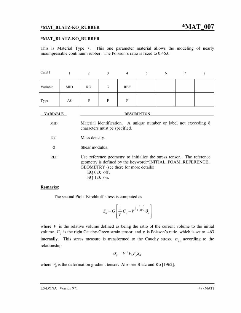
*MAT_BLATZ-KO_RUBBER *MAT_007
LS-DYNA Version 971 49 (MAT)
*MAT_BLATZ-KO_RUBBER
This is Material Type 7. This one parameter material allows the modeling of nearly incompressible continuum rubber. The Poisson’s ratio is fixed to 0.463.
Card 1 1 2 3 4 5 6 7 8
Variable MID RO G REF
Type A8 F F F
VARIABLE DESCRIPTION
MID Material identification. A unique number or label not exceeding 8 characters must be specified.
RO Mass density.
G Shear modulus.
REF Use reference geometry to initialize the stress tensor. The reference geometry is defined by the keyword:*INITIAL_FOAM_REFERENCE_ GEOMETRY (see there for more details).
EQ.0.0: off, EQ.1.0: on.
Remarks:
The second Piola-Kirchhoff stress is computed as
11 21
ij ij ijS G C VV
υ δ−= −
where V is the relative volume defined as being the ratio of the current volume to the initial volume, Cij is the right Cauchy-Green strain tensor, and v is Poisson’s ratio, which is set to .463
internally. This stress measure is transformed to the Cauchy stress, ijσ , according to the
relationship
σ ij = V −1FikFjlSlk
where Fij is the deformation gradient tensor. Also see Blatz and Ko [1962].

*MAT_008 *MAT_HIGH_EXPLOSIVE_BURN
50 (MAT) LS-DYNA Version 971
*MAT_HIGH_EXPLOSIVE_BURN
This is Material Type 8. It allows the modeling of the detonation of a high explosive. In addition an equation of state must be defined. See Wilkins [1969] and Giroux [1973].
Card 1 1 2 3 4 5 6 7 8
Variable MID RO D PCJ BETA K G SIGY
Type A8 F F F F F F F
VARIABLE DESCRIPTION
MID Material identification. A unique number or label not exceeding 8 characters must be specified.
RO Mass density.
D Detonation velocity.
PCJ Chapman-Jouget pressure.
BETA Beta burn flag, BETA (see comments below): EQ.0.0: beta + programmed burn, EQ.1.0: beta burn only, EQ.2.0: programmed burn only.
K Bulk modulus (BETA=2.0 only).
G Shear modulus (BETA=2.0 only).
SIGY yσ , yield stress (BETA=2.0 only).
Remarks:
Burn fractions, F , which multiply the equations of states for high explosives, control the release of chemical energy for simulating detonations. At any time, the pressure in a high explosive element is given by:
p = Fpeos (V, E)
where peos , is the pressure from the equation of state (either types 2, 3, or 14), V is the relative volume, and E is the internal energy density per unit initial volume.
In the initialization phase, a lighting time tl is computed for each element by dividing the distance from the detonation point to the center of the element by the detonation velocity D. If

*MAT_HIGH_EXPLOSIVE_BURN *MAT_008
LS-DYNA Version 971 51 (MAT)
multiple detonation points are defined, the closest detonation point determines tl. The burn fraction F is taken as the maximum
F = max(F1, F2 )
where
( )max
1
2if
3
0 if
l el
e
l
t t DAt t
v
F
t t
−>
=≤
2
1
1 CJ
VF
Vβ −= =
−
where VCJ is the Chapman-Jouguet relative volume and t is current time. If F exceeds 1, it is reset to 1. This calculation of the burn fraction usually requires several time steps for F to reach unity, thereby spreading the burn front over several elements. After reaching unity, F is held constant. This burn fraction calculation is based on work by Wilkins [1964] and is also discussed by Giroux [1973].
If the beta burn option is used, BETA=1.0, any volumetric compression will cause detonation and
F = F2
and F1 is not computed.
If programmed burn is used, BETA=2.0, the explosive model will behave as an elastic perfectly plastic material if the bulk modulus, shear modulus, and yield stress are defined. Therefore, with this option the explosive material can compress without causing detonation.
As an option, the high explosive material can behave as an elastic perfectly-plastic solid prior to detonation. In this case we update the stress tensor, to an elastic trial stress, *sij
n+1 ,
1* 2n nij ij ip pj jp pi ijs s s s G dtΩ Ω ε+ ′= + + +
where G is the shear modulus, and ijε ′ is the deviatoric strain rate. The von Mises yield
condition is given by: 2
2 3yJ
σφ = −
where the second stress invariant, J2 , is defined in terms of the deviatoric stress components as

*MAT_008 *MAT_HIGH_EXPLOSIVE_BURN
52 (MAT) LS-DYNA Version 971
2
1
2 ij ijJ s s=
and the yield stress is σy . If yielding has occurred, i.e., φ > 0 , the deviatoric trial stress is scaled
to obtain the final deviatoric stress at time n+1:
1 1
2
*3
yn nij ijs s
J
σ+ +=
If φ ≤ 0 , then
sijn+1 = *sij
n+1
Before detonation pressure is given by the expression
11
11n
np KV
++= −
where K is the bulk modulus. Once the explosive material detonates:
sijn+1 = 0
and the material behaves like a gas.
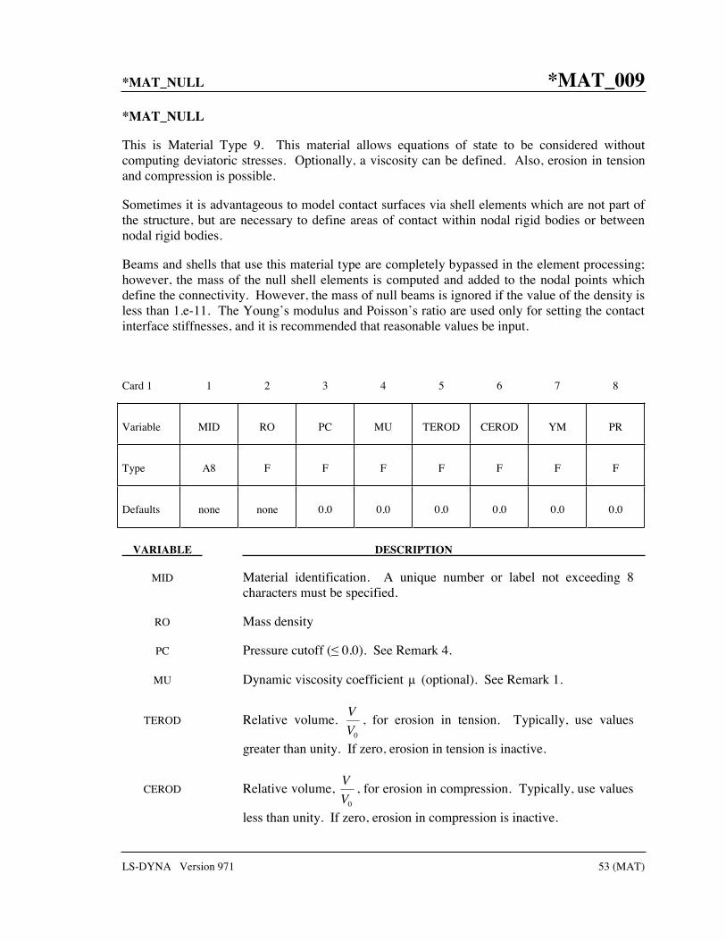
*MAT_NULL *MAT_009
LS-DYNA Version 971 53 (MAT)
*MAT_NULL
This is Material Type 9. This material allows equations of state to be considered without computing deviatoric stresses. Optionally, a viscosity can be defined. Also, erosion in tension and compression is possible.
Sometimes it is advantageous to model contact surfaces via shell elements which are not part of the structure, but are necessary to define areas of contact within nodal rigid bodies or between nodal rigid bodies.
Beams and shells that use this material type are completely bypassed in the element processing; however, the mass of the null shell elements is computed and added to the nodal points which define the connectivity. However, the mass of null beams is ignored if the value of the density is less than 1.e-11. The Young’s modulus and Poisson’s ratio are used only for setting the contact interface stiffnesses, and it is recommended that reasonable values be input.
Card 1 1 2 3 4 5 6 7 8
Variable MID RO PC MU TEROD CEROD YM PR
Type A8 F F F F F F F
Defaults none none 0.0 0.0 0.0 0.0 0.0 0.0
VARIABLE DESCRIPTION
MID Material identification. A unique number or label not exceeding 8 characters must be specified.
RO Mass density
PC Pressure cutoff ( 0.0). See Remark 4.
MU Dynamic viscosity coefficient (optional). See Remark 1.
TEROD Relative volume. 0
V
V, for erosion in tension. Typically, use values
greater than unity. If zero, erosion in tension is inactive.
CEROD Relative volume, 0
V
V, for erosion in compression. Typically, use values
less than unity. If zero, erosion in compression is inactive.

*MAT_009 *MAT_NULL
54 (MAT) LS-DYNA Version 971
VARIABLE DESCRIPTION
YM Young’s modulus (used for null beams and shells only)
PR Poisson’s ratio (used for null beams and shells only)
Remarks:
1. The null material must be used with an equation-of-state. Pressure cutoff is negative in tension. A (deviatoric) viscous stress of the form
2ij ijσ με′ ′=
2 2
1N Ns
m m s
is computed for nonzero μ where ijε ′ is the deviatoric strain rate. μ is the dynamic
viscosity. For example, in SI unit system, μ may have a unit of [Pa*s].
2. Null material has no shear stiffness and hourglass control must be used with great care. In some applications, the default hourglass coefficient might lead to significant energy losses. In general for fluid(s), the hourglass coefficient QM should be small (in the range 1.0E-4 to 1.0E-6 in the SI unit system for the standard default IHQ choice).
3. The Null material has no yield strength and behaves in a fluid-like manner.
4. The cut-off pressure, PC, must be defined to allow for a material to “numerically” cavitate. In other words, when a material undergoes dilatation above certain magnitude, it should no longer be able to resist this dilatation. Since dilatation stress or pressure is negative, setting PC limit to a very small negative number would allow for the material to cavitate once the pressure in the material goes below this negative value.

*MAT_ELASTIC_PLASTIC_HYDRO *MAT_010
LS-DYNA Version 971 55 (MAT)
*MAT_ELASTIC_PLASTIC_HYDRO_{OPTION}
This is Material Type 10. This material allows the modeling of an elastic-plastic hydrodynamic material.
Available options include:
<BLANK>
SPALL
The keyword card can appear in two ways:
*MAT_ELASTIC_PLASTIC_HYDRO or MAT_010
*MAT_ELASTIC_PLASTIC_HYDRO_SPALL or MAT_010_SPALL
Card 1 1 2 3 4 5 6 7 8
Variable MID RO G SIGY EH PC FS CHARL
Type A8 F F F F F F F
Default none none none 0.0 0.0 -∞ 0.0 0.0
Define this card if and only if the SPALL option is specified.
Optional 1 2 3 4 5 6 7 8
Variable A1 A2 SPALL
Type F F F
Card 2
Variable EPS1 EPS2 EPS3 EPS4 EPS5 EPS6 EPS7 EPS8
Type F F F F F F F F

*MAT_010 *MAT_ELASTIC_PLASTIC_HYDRO
56 (MAT) LS-DYNA Version 971
Card 3 1 2 3 4 5 6 7 8
Variable EPS9 EPS10 EPS11 EPS12 EPS13 EPS14 EPS15 EPS16
Type F F F F F F F F
Card 4
Variable ES1 ES2 ES3 ES4 ES5 ES6 ES7 ES8
Type F F F F F F F F
Card 5
Variable ES9 ES10 ES11 ES12 ES13 ES14 ES15 ES16
Type F F F F F F F F
VARIABLE DESCRIPTION
MID Material identification. A unique number or label not exceeding 8 characters must be specified.
RO Mass density.
G Shear modulus.
SIGY Yield stress, see comment below.
EH Plastic hardening modulus, see definition below.
PC Pressure cutoff ( 0.0). If zero, a cutoff of -∞ is assumed.
FS Failure strain for erosion.
CHARL Characteristic element thickness for deletion. This applies to 2D solid elements that lie on a boundary of a part. If the boundary element thins down due to stretching or compression, and if it thins to a value less than CHARL, the element will be deleted. The primary application of this option is to predict the break-up of axisymmetric shaped charge jets.

*MAT_ELASTIC_PLASTIC_HYDRO *MAT_010
LS-DYNA Version 971 57 (MAT)
VARIABLE DESCRIPTION
A1 Linear pressure hardening coefficient.
A2 Quadratic pressure hardening coefficient.
SPALL Spall type: EQ.0.0: default set to “1.0”, EQ.1.0: p > pmin,
EQ.2.0: if σ max -p min element spalls and tension, p < 0, is never allowed,
EQ.3.0: p < -pmin element spalls and tension, p < 0, is never allowed.
EPS Effective plastic strain (True). Define up to 16 values. Care must be taken that the full range of strains expected in the analysis is covered. Linear extrapolation is used if the strain values exceed the maximum input value.
ES Effective stress. Define up to 16 values.
Remarks:
If ES and EPS are undefined, the yield stress and plastic hardening modulus are taken from SIGY and EH. In this case, the bilinear stress-strain curve shown in Figure 3.1. is obtained with hardening parameter, =1. The yield strength is calculated as
( ) [ ]0 1 2 max ,0py hE a pa pσ σ ε= + + +
The quantity Eh is the plastic hardening modulus defined in terms of Young’s modulus, E, and the tangent modulus, Et , as follows
th
t
E EE
E E=
− .
and p is the pressure taken as positive in compression.
If ES and EPS are specified, a curve like that shown in Figure 10.1. may be defined. Effective stress is defined in terms of the deviatoric stress tensor, sij, as:
123
2 ij ijs sσ =
and effective plastic strain by: 1
2
0
2,
3
tp p pij ijD D dtε =
where t denotes time and Dijp is the plastic component of the rate of deformation tensor. In this
case the plastic hardening modulus on Card 1 is ignored and the yield stress is given as

*MAT_010 *MAT_ELASTIC_PLASTIC_HYDRO
58 (MAT) LS-DYNA Version 971
( ) ,py fσ ε=
where the value for ( )pf ε is found by interpolation from the data curve.
A choice of three spall models is offered to represent material splitting, cracking, and failure under tensile loads. The pressure limit model, SPALL=1, limits the hydrostatic tension to the specified value, pcut. If pressures more tensile than this limit are calculated, the pressure is reset to pcut. This option is not strictly a spall model, since the deviatoric stresses are unaffected by the pressure reaching the tensile cutoff, and the pressure cutoff value, pcut, remains unchanged throughout the analysis. The maximum principal stress spall model, SPALL=2, detects spall if the maximum principal stress, σ max, exceeds the limiting value -pcut. Note that the negative sign is required because pcut is measu red positive in compression, while σ max is positive in tension. Once spall is detected with this model, the deviatoric stresses are reset to zero, and no hydrostatic tension (p<0) is permitted. If tensile pressures are calculated, they are reset to 0 in the spalled material. Thus, the spalled material behaves as a rubble or incohesive material. The hydrostatic tension spall model, SPALL=3, detects spall if the pressure becomes more tensile than the specified limit, pcut. Once spall is detected the deviatoric stresses are reset to zero, and nonzero values of pressure are required to be compressive (positive). If hydrostatic tension (p<0) is subsequently calculated, the pressure is reset to 0 for that element.
This model is applicable to a wide range of materials, including those with pressure-dependent yield behavior. The use of 16 points in the yield stress versus effective plastic strain curve allows complex post-yield hardening behavior to be accurately represented. In addition, the incorporation of an equation of state permits accurate modeling of a variety of different materials. The spall model options permit incorporation of material failure, fracture, and disintegration effects under tensile loads.
Figure 10.1. Effective stress versus effective plastic strain curve.

*MAT_STEINBERG *MAT_011
LS-DYNA Version 971 59 (MAT)
*MAT_STEINBERG
This is Material Type 11. This material is available for modeling materials deforming at very high strain rates (>105) and can be used with solid elements. The yield strength is a function of temperature and pressure. An equation of state determines the pressure.
Card 1 1 2 3 4 5 6 7 8
Variable MID RO G0 SIGO BETA N GAMA SIGM
Type A8 F F F F F F F
Card 2
Variable B BP H F A TMO GAMO SA
Type F F F F F F F F
Card 3
Variable PC SPALL RP FLAG MMN MMX ECO EC1
Type F F F F F F F F
Card 4
Variable EC2 EC3 EC4 EC5 EC6 EC7 EC8 EC9
Type F F F F F F F F

*MAT_011 *MAT_STEINBERG
60 (MAT) LS-DYNA Version 971
VARIABLE DESCRIPTION
MID Material identification. A unique number or label not exceeding 8 characters must be specified.
RO Mass density.
G0 Basic shear modulus.
SIGO σo, see defining equations.
BETA β, see defining equations.
N n, see defining equations.
GAMA i , initial plastic strain, see defining equations.
SIGM σm, see defining equations.
B b, see defining equations.
BP b′, see defining equations.
H h, see defining equations.
F f, see defining equations.
A Atomic weight (if = 0.0, R′ must be defined).
TMO Tmo, see defining equations.
GAMO γo, see defining equations.
SA a, see defining equations.
PC pcut or -σf (default=-1.e+30)
SPALL Spall type: EQ. 0.0: default set to “2.0”, EQ. 1.0: p ≥ pcut,
EQ. 2.0: if σmax -pcut element spalls and tension, p < 0, is never allowed,
EQ. 3.0: p < -pcut element spalls and tension, p < 0, is never allowed.
RP R′. If R′ ≠ 0.0, A is not defined.

*MAT_STEINBERG *MAT_011
LS-DYNA Version 971 61 (MAT)
VARIABLE DESCRIPTION
FLAG Set to 1.0 for μ coefficients for the cold compression energy fit. Default is η.
MMN μmin or ηmin. Optional μ or η minimum value.
MMX μmax or ηmax. Optional μ or η maximum value.
EC0,...EC9 Cold compression energy coefficients (optional).
Remarks:
Users who have an interest in this model are encouraged to study the paper by Steinberg and Guinan which provides the theoretical basis. Another useful reference is the KOVEC user’s manual.
In terms of the foregoing input parameters, we define the shear modulus, G, before the material melts as:
13
0 1 3003
fE iE Em ii cE E
G G bpV h eR
−−−= + − −
′
where p is the pressure, V is the relative volume, Ec is the cold compression energy:
( ) ( )( ) ( )1
0 220
900 exp,
1
x
c a
R axE x pdx
xγ − −
′= −
−
x = 1 – V,
and Em is the melting energy:
( ) ( ) ( )3m c mE x E x R T x′= +
which is in terms of the melting temperature ( )mT x :
( ) ( )( )1
32
exp 2o
mom a
T axT x
V γ − −=
and the melting temperature at oρ ρ= , moT .
In the above equation R′ is defined by
RR
A
ρ′ =

*MAT_011 *MAT_STEINBERG
62 (MAT) LS-DYNA Version 971
where R is the gas constant and A is the atomic weight. If R′ is not defined, LS-DYNA computes it with R in the cm-gram-microsecond system of units.
The yield strength σy is given by:
13
0 1 3003
fEiE Em ii c
y
E Eb pV h e
Rσ σ −−−
′ ′= + − −′
if Em exceeds Ei. Here, σ0′ is given by:
( )0 0 1n
piσ σ β γ ε′ = + +
where σ0 is the initial yield stress and γi is the initial plastic strain. If the work-hardened yield
stress σ0′ exceeds σm, σ0′ is set equal to σm. After the materials melt, y and G are set to one half their initial value.
If the coefficients EC0,...,EC9 are not defined above, LS-DYNA will fit the cold compression energy to a ten term polynomial expansion either as a function of μ or η depending on the input variable, FLAG, as:
( )
( )
9
0
9
0
i ic i
i
i ic i
i
E EC
E EC
η η
μ μ
=
=
=
=
where ECi is the ith coefficient and:
1
o
o
ρηρρμρ
=
= −
A linear least squares method is used to perform the fit.
A choice of three spall models is offered to represent material splitting, cracking, and failure under tensile loads. The pressure limit model, SPALL=1, limits the hydrostatic tension to the specified value, pcut. If pressures more tensile than this limit are calculated, the pressure is reset to pcut. This option is not strictly a spall model, since the deviatoric stresses are unaffected by the pressure reaching the tensile cutoff, and the pressure cutoff value, pcut, remains unchanged throughout the analysis. The maximum principal stress spall model, SPALL=2, detects spall if the maximum principal stress, max, exceeds the limiting value -pcut. Note that the negative sign is required because pcut is measured positive in compression, while max is positive in tension. Once spall is detected with this model, the deviatoric stresses are reset to
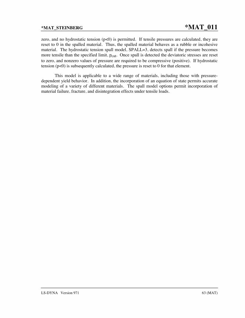
*MAT_STEINBERG *MAT_011
LS-DYNA Version 971 63 (MAT)
zero, and no hydrostatic tension (p<0) is permitted. If tensile pressures are calculated, they are reset to 0 in the spalled material. Thus, the spalled material behaves as a rubble or incohesive material. The hydrostatic tension spall model, SPALL=3, detects spall if the pressure becomes more tensile than the specified limit, pcut. Once spall is detected the deviatoric stresses are reset to zero, and nonzero values of pressure are required to be compressive (positive). If hydrostatic tension (p<0) is subsequently calculated, the pressure is reset to 0 for that element.
This model is applicable to a wide range of materials, including those with pressure-dependent yield behavior. In addition, the incorporation of an equation of state permits accurate modeling of a variety of different materials. The spall model options permit incorporation of material failure, fracture, and disintegration effects under tensile loads.

*MAT_011_LUND *MAT_STEINBERG_LUND
64 (MAT) LS-DYNA Version 971
*MAT_STEINBERG_LUND
This is Material Type 11. This material is a modification of the Steinberg model above to include the rate model of Steinberg and Lund [1989]. An equation of state determines the pressure.
The keyword cards can appear in two ways:
*MAT_STEINBERG_LUND or MAT_011_LUND
Card 1 1 2 3 4 5 6 7 8
Variable MID RO G0 SIGO BETA N GAMA SIGM
Type A8 F F F F F F F
Card 2
Variable B BP H F A TMO GAMO SA
Type F F F F F F F F
Card 3
Variable PC SPALL RP FLAG MMN MMX ECO EC1
Type F F F F F F F F
Card 4
Variable EC2 EC3 EC4 EC5 EC6 EC7 EC8 EC9
Type F F F F F F F F

*MAT_STEINBERG_LUND *MAT_011_LUND
LS-DYNA Version 971 65 (MAT)
Card 5 1 2 3 4 5 6 7 8
Variable UK C1 C2 YP YA YM
Type F F F F F F
VARIABLE DESCRIPTION
MID Material identification. A unique number or label not exceeding 8 characters must be specified.
RO Mass density.
G0 Basic shear modulus.
SIGO o, see defining equations.
BETA , see defining equations.
N n, see defining equations.
GAMA γi, initial plastic strain, see defining equations.
SIGM m, see defining equations.
B b, see defining equations.
BP b′, see defining equations.
H h, see defining equations.
F f, see defining equations.
A Atomic weight (if = 0.0, R′ must be defined).
TMO Tmo, see defining equations.
GAMO γo, see defining equations.
SA a, see defining equations.
PC pcut or -σf (default=-1.e+30)

*MAT_011_LUND *MAT_STEINBERG_LUND
66 (MAT) LS-DYNA Version 971
VARIABLE DESCRIPTION
SPALL Spall type: EQ. 0.0: default set to “2.0”, EQ. 1.0: minp p≥ ,
EQ. 2.0: if max minpσ ≥ − element spalls and tension, p 0< , is never
allowed,
EQ. 3.0: minp p< − element spalls and tension, p 0< , is never
allowed.
RP R′. If R′ ≠ 0.0, A is not defined.
FLAG Set to 1.0 for μ coefficients for the cold compression energy fit. Default is η.
MMN μmin or ηmin. Optional μ or η minimum value.
MMX μmax or ηmax. Optional μ or η maximum value.
EC0,...EC9 Cold compression energy coefficients (optional).
UK Activation energy for rate dependent model.
C1 Exponent prefactor in rate dependent model.
C2 Coefficient of drag term in rate dependent model.
YP Peierls stress for rate dependent model.
YA Athermal yield stress for rate dependent model.
YMAX Work hardening maximum for rate model.
Remarks:
This model is similar in theory to the *MAT_STEINBERG above but with the addition of rate effects. When rate effects are included, the yield stress is given by:
( ) ( ){ } ( )0
,,y T p A p
G p TY T Y f
Gσ ε ε= +
There are two imposed limits on the yield stress. The first is on the thermal yield stress:
( ) ( )1n
pA p A i maxY f Y Yε β γ ε= + + ≤
and the second is on the thermal part:
YT ≤ YP

*MAT_ISOTROPIC_ELASTIC_PLASTIC *MAT_012
LS-DYNA Version 971 67 (MAT)
*MAT_ISOTROPIC_ELASTIC_PLASTIC
This is Material Type 12. This is a very low cost isotropic plasticity model for three-dimensional solids. In the plane stress implementation for shell elements, a one-step radial return approach is used to scale the Cauchy stress tensor to if the state of stress exceeds the yield surface. This approach to plasticity leads to inaccurate shell thickness updates and stresses after yielding. This is the only model in LS-DYNA for plane stress that does not default to an iterative approach.
Card 1 2 3 4 5 6 7 8
Variable MID RO G SIGY ETAN BULK
Type A8 F F F F F
VARIABLE DESCRIPTION
MID Material identification. A unique number or label not exceeding 8 characters must be specified.
RO Mass density.
G Shear modulus.
SIGY Yield stress.
ETAN Plastic hardening modulus.
BULK Bulk modulus, K.
Remarks:
Here the pressure is integrated in time
iip K ε= −
where iiε is the volumetric strain rate.

*MAT_013 *MAT_ISOTROPIC_ELASTIC_FAILURE
68 (MAT) LS-DYNA Version 971
*MAT_ISOTROPIC_ELASTIC_FAILURE
This is Material Type 13. This is a non-iterative plasticity with simple plastic strain failure model.
Card 1 1 2 3 4 5 6 7 8
Variable MID RO G SIGY ETAN BULK
Type A8 F F F F F
Default None none none none 0.0 none
Card 2
Variable EPF PRF REM TREM
Type F F F F
Default None 0.0 0.0 0.0
VARIABLE DESCRIPTION
MID Material identification. A unique number or label not exceeding 8 characters must be specified.
RO Mass density.
G Shear modulus.
SIGY Yield stress.
ETAN Plastic hardening modulus.
BULK Bulk modulus.
EPF Plastic failure strain.
PRF Failure pressure ( ≤ 0.0).

*MAT_ISOTROPIC_ELASTIC_FAILURE *MAT_013
LS-DYNA Version 971 69 (MAT)
VARIABLE DESCRIPTION
REM Element erosion option: EQ.0.0: failed element eroded after failure, NE.0.0: element is kept, no removal except by Δt below.
TREM Δt for element removal: EQ.0.0: Δt is not considered (default), GT.0.0: element eroded if element time step size falls below Δt.
Remarks:
When the effective plastic strain reaches the failure strain or when the pressure reaches the failure pressure, the element loses its ability to carry tension and the deviatoric stresses are set to zero, i.e., the material behaves like a fluid. If Δt for element removal is defined the element removal option is ignored.
The element erosion option based on Δt must be used cautiously with the contact options. Nodes to surface contact is recommended with all nodes of the eroded brick elements included in the node list. As the elements are eroded the mass remains and continues to interact with the master surface.

*MAT_014 *MAT_SOIL_AND_FOAM_FAILURE
70 (MAT) LS-DYNA Version 971
*MAT_SOIL_AND_FOAM_FAILURE
This is Material Type 14. The input for this model is the same as for *MATERIAL_SOIL_ AND_FOAM (Type 5); however, when the pressure reaches the failure pressure, the element loses its ability to carry tension. It should be used only in situations when soils and foams are confined within a structure or when geometric boundaries are present.

*MAT_JOHNSON_COOK *MAT_015
LS-DYNA Version 971 71 (MAT)
*MAT_JOHNSON_COOK
This is Material Type 15. The Johnson/Cook strain and temperature sensitive plasticity is sometimes used for problems where the strain rates vary over a large range and adiabatic temperature increases due to plastic heating cause material softening. When used with solid elements this model requires an equation-of-state. If thermal effects and damage are unimportant, the much less expensive *MAT_SIMPLIFIED_JOHNSON_COOK model is recommended. The simplified model can be used with beam elements.
Card 1 1 2 3 4 5 6 7 8
Variable MID RO G E PR DTF VP RATEOP
Type A8 F F F F F F F
Default none none none none none 0.0 0.0 0.0
Card 2
Variable A B N C M TM TR EPSO
Type F F F F F F F F
Default none 0.0 0.0 0.0 none none none none
Card 3
Variable CP PC SPALL IT D1 D2 D3 D4
Type F F F F F F F F
Default none 0.0 2.0 0.0 0.0 0.0 0.0 0.0

*MAT_015 *MAT_JOHNSON_COOK
72 (MAT) LS-DYNA Version 971
Card 4 1 2 3 4 5 6 7 8
Variable D5 C2/P
Type F F
Default 0.0 0.0
VARIABLE DESCRIPTION
MID Material identification. A unique number or label not exceeding 8 characters must be specified.
RO Mass density
G Shear modulus
E Young’s Modulus (shell elements only)
PR Poisson’s ratio (shell elements only)
DTF Minimum time step size for automatic element deletion (shell elements)
VP Formulation for rate effects: EQ.0.0: Scale yield stress (default), EQ.1.0: Viscoplastic formulation.
RATEOP Optional forms of strain-rate term: EQ.0.0: Log-Linear Johnson-Cook (default), EQ.1.0: Log-Quadratic Huh-Kang (2 parameters), EQ.2.0: Exponential Allen-Rule-Jones, EQ.3.0: Exponential Cowper-Symonds (2 parameters).
A See equations below.
B See equations below.
N See equations below.
C See equations below.
M See equations below.
TM Melt temperature

*MAT_JOHNSON_COOK *MAT_015
LS-DYNA Version 971 73 (MAT)
VARIABLE DESCRIPTION
TR Room temperature
EPSO Quasi-static threshold strain rate. Ideally, this value represents the highest strain rate for which no rate adjustment to the flow stress is needed, and is input in units of 1/model time units. For example, if strain rate effects on the flow stress first become apparent at strain rates greater than 1E-02 seconds-1 and the system of units for the model input is kg, mm, msec, then EPSO should be set to 1E-05 [msec-1]
CP Specific heat (superseded by heat capacity in *MAT_THERMAL_OPTION if a coupled thermal/structural analysis)
PC Failure stress or pressure cutoff (pmin < 0.0)
SPALL Spall type: EQ. 0.0: default set to “2.0”, EQ. 1.0: p ≥ pmin,
EQ. 2.0: if σmax -pmin element spalls and tension, p < 0, is never allowed, EQ. 3.0: p < -pmin element spalls and tension, p < 0, is never allowed.
IT Plastic strain iteration option. This input applies to solid elements only since it is always necessary to iterate for the shell element plane stress condition.
EQ. 0.0: no iterations (default), EQ. 1.0: accurate iterative solution for plastic strain. Much more
expensive than default.
D1-D5 Failure parameters, see equations below.
C2/P Optional strain-rate parameter for Huh-Kang (C2) or Cowper-Symonds (P) forms; see equations below.
Remarks:
Johnson and Cook express the flow stress as
( ) ( )1 ln * 1np m
y A B c Tσ ε ε= + + − ∗
where
A, B, C, n, and m = input constants
pε effective plastic strain

*MAT_015 *MAT_JOHNSON_COOK
74 (MAT) LS-DYNA Version 971
For VP=0,
.
εε∗ =EPSO
effective total strain rate normalized by quasi-static
threshold rate
For VP=1, p
EPSO
εε ∗ = effective plastic strain rate normalized by quasi-static
threshold rate
T* = homologous temperature = room
melt room
T T
T T
−−
Constants for a variety of materials are provided in Johnson and Cook [1983]. A fully viscoplastic formulation is optional (VP) which incorporates the rate equations within the yield surface. An additional cost is incurred but the improvement is that results can be dramatic.
Due to nonlinearity in the dependence of flow stress on plastic strain, an accurate value of the flow stress requires iteration for the increment in plastic strain. However, by using a Taylor series expansion with linearization about the current time, we can solve for σy with sufficient accuracy to avoid iteration.
The strain at fracture is given by
*1 2 3 4 5exp 1 ln 1f D D D D D Tε σ ε∗ ∗= + + +
where σ* is the ratio of pressure divided by effective stress
eff
pσσ
∗ =
Fracture occurs when the damage parameter
p
fD
εε
Δ=
reaches the value of 1.
A choice of three spall models is offered to represent material splitting, cracking, and failure under tensile loads. The pressure limit model limits the minimum hydrostatic pressure to the specified value, p ≥ pmin . If pressures more tensile than this limit are calculated, the pressure is reset to pmin . This option is not strictly a spall model since the deviatoric stresses are unaffected by the pressure reaching the tensile cutoff and the pressure cutoff value pmin remains unchanged throughout the analysis. The maximum principal stress spall model detects spall if the maximum principal stress, σmax , exceeds the limiting value σ p . Once spall is detected with
this model, the deviatoric stresses are reset to zero and no hydrostatic tension is permitted. If tensile pressures are calculated, they are reset to 0 in the spalled material. Thus, the spalled material behaves as rubble. The hydrostatic tension spall model detects spall if the pressure

*MAT_JOHNSON_COOK *MAT_015
LS-DYNA Version 971 75 (MAT)
becomes more tensile than the specified limit, pmin . Once spall is detected, the deviatoric stresses are set to zero and the pressure is required to be compressive. If hydrostatic tension is calculated then the pressure is reset to 0 for that element.
In addition to the above failure criterion, this material model also supports a shell element deletion criterion based on the maximum stable time step size for the element, Δtmax . Generally, Δtmax goes down as the element becomes more distorted. To assure stability of time integration, the global LS-DYNA time step is the minimum of the Δtmax values calculated for all elements in the model. Using this option allows the selective deletion of elements whose time step Δtmax has fallen below the specified minimum time step, Δtcrit . Elements which are severely distorted often indicate that material has failed and supports little load, but these same elements may have very small time steps and therefore control the cost of the analysis. This option allows these highly distorted elements to be deleted from the calculation, and, therefore, the analysis can proceed at a larger time step, and, thus, at a reduced cost. Deleted elements do not carry any load, and are deleted from all applicable slide surface definitions. Clearly, this option must be judiciously used to obtain accurate results at a minimum cost.
Material type 15 is applicable to the high rate deformation of many materials including most metals. Unlike the Steinberg-Guinan model, the Johnson-Cook model remains valid down to lower strain rates and even into the quasistatic regime. Typical applications include explosive metal forming, ballistic penetration, and impact.
Optional Strain Rate Forms
The standard Johnson-Cook strain rate term is linear in the logarithim of the strain rate:
1 ln *C ε+
Some additional data fiting capability can be obtained by using the quadratic form proposed by Huh & Kang [2002]:
( )221 ln * ln *C Cε ε+ +
Two additional exponential forms are available, one due to Allen, Rule & Jones [1997]
( )*cε
and the other a Cowper-Symonds-like [1958] form:
1
1p P
eff
C
ε+
The three additional rate forms (RATEOP=1,2, or 3) are currently available for solid & shell elements but only when the viscoplastic rate option is active (VP=1). See Huh and Kang [2002], Allen, Rule, and Jones [1997], and Cowper and Symonds [1958].

*MAT_016 *MAT_PSEUDO_TENSOR
76 (MAT) LS-DYNA Version 971
*MAT_PSEUDO_TENSOR
This is Material Type 16. This model has been used to analyze buried steel reinforced concrete structures subjected to impulsive loadings.
Card 1 1 2 3 4 5 6 7 8
Variable MID RO G PR
Type A8 F F F
Default none none none none
Card 2
Variable SIGF A0 A1 A2 A0F A1F B1 PER
Type F F F F F F F F
Default 0.0 0.0 0.0 0.0 0.0 0.0 0.0 0.0
Card 3
Variable ER PRR SIGY ETAN LCP LCR
Type F F F F F F
Default 0.0 0.0 none 0.0

*MAT_PSEUDO_TENSOR *MAT_016
LS-DYNA Version 971 77 (MAT)
Card 4 1 2 3 4 5 6 7 8
Variable X1 X2 X3 X4 X5 X6 X7 X8
Type F F F F F F F F
Default
Card 5
Variable X9 X10 X11 X12 X13 X14 X15 X16
Type F F F F F F F F
Default
Card 6
Variable YS1 YS2 YS3 YS4 YS5 YS6 YS7 YS8
Type F F F F F F F F
Default
Card 7
Variable YS9 YS10 YS11 YS12 YS13 YS14 YS15 YS16
Type F F F F F F F F
Default

*MAT_016 *MAT_PSEUDO_TENSOR
78 (MAT) LS-DYNA Version 971
VARIABLE DESCRIPTION
MID Material identification. A unique number or label not exceeding 8 characters must be specified.
RO Mass density.
G Shear modulus.
PR Poisson’s ratio.
SIGF Tensile cutoff (maximum principal stress for failure).
A0 Cohesion.
A1 Pressure hardening coefficient.
A2 Pressure hardening coefficient.
A0F Cohesion for failed material.
A1F Pressure hardening coefficient for failed material.
B1 Damage scaling factor (or exponent in Mode II.C).
PER Percent reinforcement.
ER Elastic modulus for reinforcement.
PRR Poisson’s ratio for reinforcement.
SIGY Initial yield stress.
ETAN Tangent modulus/plastic hardening modulus.
LCP Load curve ID giving rate sensitivity for principal material, see *DEFINE_CURVE.
LCR Load curve ID giving rate sensitivity for reinforcement, see *DEFINE_CURVE.
X Effective plastic strain, damage, or pressure. See discussion below.
YS Yield stress (Mode I) or scale factor (Mode II.B or II.C).
Remarks:
This model can be used in two major modes - a simple tabular pressure-dependent yield surface, and a potentially complex model featuring two yield versus pressure functions with the means of migrating from one curve to the other. For both modes, load curve LCP is taken to be a

*MAT_PSEUDO_TENSOR *MAT_016
LS-DYNA Version 971 79 (MAT)
strain rate multiplier for the yield strength. Note that this model must be used with equation-of-state type 8 or 9.
Response Mode I. Tabulated Yield Stress Versus Pressure
This model is well suited for implementing standard geologic models like the Mohr-Coulomb yield surface with a Tresca limit, as shown in Figure 16.1. Examples of converting conventional triaxial compression data to this type of model are found in (Desai and Siriwardane, 1984). Note that under conventional triaxial compression conditions, the LS-DYNA input
corresponds to an ordinate of 1 3σ σ− rather than the more widely used 1 3
2
σ σ−, where 1σ is the
maximum principal stress and 3σ is the minimum principal stress.
This material combined with equation-of-state type 9 (saturated) has been used very successfully to model ground shocks and soil-structure interactions at pressures up to 100kbars (approximately 1.5 x 10⁶ psi).
Figure 16.1. Mohr-Coulomb surface with a Tresca limit.
To invoke Mode I of this model, set a0, a1, a2, b1, a0f, and a1f to zero. The tabulated values of pressure should then be specified on cards 4 and 5, and the corresponding values of yield stress should be specified on cards 6 and 7. The parameters relating to reinforcement properties, initial yield stress, and tangent modulus are not used in this response mode, and should be set to zero.

*MAT_016 *MAT_PSEUDO_TENSOR
80 (MAT) LS-DYNA Version 971
Simple tensile failure Note that a1f is reset internally to 1/3 even though it is input as zero; this defines a failed material curve of slope 3p, where p denotes pressure (positive in compression). In this case the yield strength is taken from the tabulated yield vs. pressure curve until the maximum principal stress( 1σ ) in the element exceeds the tensile cut-off ( cutσ ). For every time step that 1 cutσ σ> the
yield strength is scaled back by a fraction of the distance between the two curves until after 20 time steps the yield strength is defined by the failed curve. The only way to inhibit this feature is to set cutσ arbitrarily large.
Response Mode II. Two Curve Model with Damage and Failure
This approach uses two yield versus pressure curves of the form
01 2
y
pa
a a pσ = +
+
The upper curve is best described as the maximum yield strength curve and the lower curve is the failed material curve. There are a variety of ways of moving between the two curves and each is discussed below.
Figure 16.2. Two-curve concrete model with damage and failure.
MODE II. A: Simple tensile failure Define a0, a1, a2, a0f and a1f, set b1 to zero, and leave cards 4 through 7 blank. In this case the yield strength is taken from the maximum yield curve until the maximum principal stress ( 1σ ) in the element exceeds the tensile cut-off ( cutσ ). For every time step that 1 cutσ σ>the yield strength is scaled back by a fraction of the distance between the two curves until after 20 time steps the yield strength is defined by the failure curve.

*MAT_PSEUDO_TENSOR *MAT_016
LS-DYNA Version 971 81 (MAT)
Mode II.B: Tensile failure plus plastic strain scaling Define a0, a1, a2, a0f and a1f, set b1 to zero, and user cards 4 through 7 to define a scale factor, η, versus effective plastic strain. LS-DYNA evaluates η at the current effective plastic strain and then calculated the yield stress as
max( )yield failed failedσ σ η σ σ= + −
where maxσ and failedσ are found as shown in Figure 16.2. This yield strength is then subject to
scaling for tensile failure as described above. This type of model allows the description of a strain hardening or softening material such as concrete.
Mode II.C: Tensile failure plus damage scaling The change in yield stress as a function of plastic strain arises from the physical mechanisms such as internal cracking, and the extent of this cracking is affected by the hydrostatic pressure when the cracking occurs. This mechanism gives rise to the "confinement" effect on concrete behavior. To account for this phenomenon, a "damage" function was defined and incorporated. This damage function is given the form:
1
0
1
p b
p
cut
pd
ε
λ εσ
−
= +
Define a0, a1, a2, a0f and a1f, and b1. Cards 4 though 7 now give as a function of and scale the yield stress as
( )maxyield failed failedσ σ η σ σ= + −
and then apply any tensile failure criteria.
Mode II Concrete Model Options Material Type 16 Mode II provides for the automatic internal generation of a simple "generic" model from concrete if A0 is negative then SIGF is assumed to be the unconfined concrete compressive strength, cf
′ and –A0 is assumed to be a conversion factor from LS-
DYNA pressure units to psi. (For example, if the model stress units are MPa, A0 should be set to –145.) In this case the parameter values generated internally are

*MAT_016 *MAT_PSEUDO_TENSOR
82 (MAT) LS-DYNA Version 971
'
1'2 3
'
0
1
2 '
0
1
1.70
41
31
3
0
0.385
c
ccut
c
c
f
f
f SIGF
f
A
fa
a
af
a
a
σ
=
=−
=
=
=
=
=
Note that these a0f and a1f defaults will be overridden by non zero entries on Card 3. If plastic strain or damage scaling is desired, Cards 5 through 8 and b1 should be specified in the input. When a0 is input as a negative quantity, the equation-of-state can be given as 0 and a trilinear EOS Type 8 model will be automatically generated from the unconfined compressive strength and Poisson's ratio. The EOS 8 model is a simple pressure versus volumetric strain model with no internal energy terms, and should give reasonable results for pressures up to 5kbar (approximately 75,000 psi).
Mixture model A reinforcement fraction, rf , can be defined along with properties of the reinforcement
material. The bulk modulus, shear modulus, and yield strength are then calculated from a simple mixture rule, i.e., for the bulk modulus the rule gives:
( )1 r m r rK f K f K= − +
where mK and rK are the bulk moduli for the geologic material and the reinforcement material,
respectively. This feature should be used with caution. It gives an isotropic effect in the material instead of the true anisotropic material behavior. A reasonable approach would be to use the mixture elements only where the reinforcing exists and plain elements elsewhere. When the mixture model is being used, the strain rate multiplier for the principal material is taken from load curve N1 and the multiplier for the reinforcement is taken from load curve N2.
A Suggestion The LLNL DYNA3D manual from 1991 [Whirley and Hallquist] suggests using the damage function (Mode II.C.) in Material Type 16 with the following set of parameters:
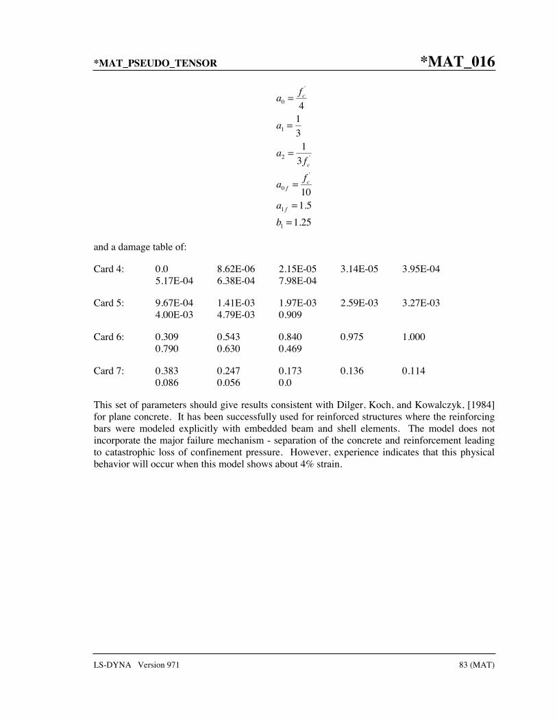
*MAT_PSEUDO_TENSOR *MAT_016
LS-DYNA Version 971 83 (MAT)
'
0
1
2 '
'
0
1
1
41
31
3
101.5
1.25
c
c
cf
f
fa
a
af
fa
a
b
=
=
=
=
=
=
and a damage table of:
Card 4: 0.0 8.62E-06 2.15E-05 3.14E-05 3.95E-04 5.17E-04 6.38E-04 7.98E-04
Card 5: 9.67E-04 1.41E-03 1.97E-03 2.59E-03 3.27E-03 4.00E-03 4.79E-03 0.909
Card 6: 0.309 0.543 0.840 0.975 1.000 0.790 0.630 0.469
Card 7: 0.383 0.247 0.173 0.136 0.114 0.086 0.056 0.0
This set of parameters should give results consistent with Dilger, Koch, and Kowalczyk, [1984] for plane concrete. It has been successfully used for reinforced structures where the reinforcing bars were modeled explicitly with embedded beam and shell elements. The model does not incorporate the major failure mechanism - separation of the concrete and reinforcement leading to catastrophic loss of confinement pressure. However, experience indicates that this physical behavior will occur when this model shows about 4% strain.

*MAT_017 *MAT_ORIENTED_CRACK
84 (MAT) LS-DYNA Version 971
*MAT_ORIENTED_CRACK
This is Material Type 17. This material may be used to model brittle materials which fail due to large tensile stresses.
Card 1 1 2 3 4 5 6 7 8
Variable MID RO E PR SIGY ETAN FS PRF
Type A8 F F F F F F F
Default none None none none none 0.0 none 0.0
VARIABLE DESCRIPTION
MID Material identification. A unique number or label not exceeding 8 characters must be specified.
RO Mass density.
E Young’s modulus.
PR Poisson’s ratio.
SIGY Yield stress.
ETAN Plastic hardening modulus.
FS Fracture stress.
PRF Failure or cutoff pressure (≤ 0.0).
Remarks:
This is an isotropic elastic-plastic material which includes a failure model with an oriented crack. The von Mises yield condition is given by:
2
2 3yJ
σφ = −
where the second stress invariant, 2J , is defined in terms of the deviatoric stress components as
2
1
2 ij ijJ s s=

*MAT_ORIENTED_CRACK *MAT_017
LS-DYNA Version 971 85 (MAT)
and the yield stress, yσ , is a function of the effective plastic strain, peffε , and the plastic hardening
modulus, pE :
0p
y p effEσ σ ε= +
The effective plastic strain is defined as:
0
tp p
eff effdε ε=
where 2
3p p p
eff ij ijd d dε ε ε=
and the plastic tangent modulus is defined in terms of the input tangent modulus, tE , as
tp
t
EEE
E E=
−
Pressure in this model is found from evaluating an equation of state. A pressure cutoff can be defined such that the pressure is not allowed to fall below the cutoff value.
The oriented crack fracture model is based on a maximum principal stress criterion. When the maximum principal stress exceeds the fracture stress, fσ , the element fails on a plane
perpendicular to the direction of the maximum principal stress. The normal stress and the two shear stresses on that plane are then reduced to zero. This stress reduction is done according to a delay function that reduces the stresses gradually to zero over a small number of time steps. This delay function procedure is used to reduce the ringing that may otherwise be introduced into the system by the sudden fracture.
After a tensile fracture, the element will not support tensile stress on the fracture plane, but in compression will support both normal and shear stresses. The orientation of this fracture surface is tracked throughout the deformation, and is updated to properly model finite deformation effects. If the maximum principal stress subsequently exceeds the fracture stress in another direction, the element fails isotropically. In this case the element completely loses its ability to support any shear stress or hydrostatic tension, and only compressive hydrostatic stress states are possible. Thus, once isotropic failure has occurred, the material behaves like a fluid.
This model is applicable to elastic or elastoplastic materials under significant tensile or shear loading when fracture is expected. Potential applications include brittle materials such as ceramics as well as porous materials such as concrete in cases where pressure hardening effects are not significant.

*MAT_018 *MAT_POWER_LAW_PLASTICITY
86 (MAT) LS-DYNA Version 971
*MAT_POWER_LAW_PLASTICITY
This is Material Type 18. This is an isotropic plasticity model with rate effects which uses a power law hardening rule.
Card 1 1 2 3 4 5 6 7 8
Variable MID RO E PR K N SRC SRP
Type A8 F F F F F F F
Default none none none none none none 0.0 0.0
Card 2
Variable SIGY VP
Type F F
Default 0.0 0.0
VARIABLE DESCRIPTION
MID Material identification. A unique number or label not exceeding 8 characters must be specified.
RO Mass density.
E Young’s modulus.
PR Poisson’s ratio.
K Strength coefficient.
N Hardening exponent.
SRC Strain rate parameter, C, if zero, rate effects are ignored.
SRP Strain rate parameter, P, if zero, rate effects are ignored.

*MAT_POWER_LAW_PLASTICITY *MAT_018
LS-DYNA Version 971 87 (MAT)
VARIABLE DESCRIPTION
SIGY Optional input parameter for defining the initial yield stress, yσ .
Generally, this parameter is not necessary and the strain to yield is calculated as described below.
LT.0.02: yp SIGYε = GE.0.02: See below.
VP Formulation for rate effects: EQ.0.0: Scale yield stress (default), EQ.1.0: Viscoplastic formulation.
Remarks:
Elastoplastic behavior with isotropic hardening is provided by this model. The yield stress, σy, is a function of plastic strain and obeys the equation:
( )nn py ypk kσ ε ε ε= = +
where ypε is the elastic strain to yield and pε is the effective plastic strain (logarithmic). If
SIGY is set to zero, the strain to yield if found by solving for the intersection of the linearly elastic loading equation with the strain hardening equation:
n
E
k
σ εσ ε
=
=
which gives the elastic strain at yield as:
1
1n
yp
E
kε
−=
If SIGY yield is nonzero and greater than 0.02 then:
1
ny
yp k
σε =
Strain rate is accounted for using the Cowper and Symonds model which scales the yield stress with the factor
1
1p
C
ε+
where ε is the strain rate. A fully viscoplastic formulation is optional which incorporates the Cowper and Symonds formulation within the yield surface. An additional cost is incurred but the improvement is results can be dramatic.

*MAT_019 *MAT_STRAIN_RATE_DEPENDENT_PLASTICITY
88 (MAT) LS-DYNA Version 971
*MAT_STRAIN_RATE_DEPENDENT_PLASTICITY
This is Material Type 19. A strain rate dependent material can be defined. For an alternative, see Material Type 24. Required is a curve for the yield stress versus the effective strain rate. Optionally, Young’s modulus and the tangent modulus can also be defined versus the effective strain rate. Also, optional failure of the material can be defined either by defining a von Mises stress at failure as a function of the effective strain rate (valid for solids/shells/thick shells) or by defining a minimum time step size (only for shells).
Card 1 1 2 3 4 5 6 7 8
Variable MID RO E PR VP
Type A8 F F F F
Default none none none none 0.0
Card 2
Variable LC1 ETAN LC2 LC3 LC4 TDEL RDEF
Type F F F F F F F
Default none 0.0 0.0 0.0 0.0 0.0 0.0
VARIABLE DESCRIPTION
MID Material identification. A unique number or label not exceeding 8 characters must be specified.
RO Mass density.
E Young’s modulus.
PR Poisson’s ratio.
VP Formulation for rate effects: EQ.0.0: Scale yield stress (default), EQ.1.0: Viscoplastic formulation (recommended).

*MAT_STRAIN_RATE_DEPENDENT_PLASTICITY *MAT_019
LS-DYNA Version 971 89 (MAT)
VARIABLE DESCRIPTION
LC1 Load curve ID defining the yield stress σ0 as a function of the effective strain rate.
ETAN Tangent modulus, Et
LC2 Load curve ID defining Young’s modulus as a function of the effective strain rate (available only when VP=0; not recommended).
LC3 Load curve ID defining tangent modulus as a function of the effective strain rate (optional).
LC4 Load curve ID defining von Mises stress at failure as a function of the effective strain rate (optional).
TDEL Minimum time step size for automatic element deletion. Use for shells only.
RDEF Redefinition of failure curve: EQ.1.0: Effective plastic strain, EQ.2.0: Maximum principal stress.
Remarks:
In this model, a load curve is used to describe the yield strength 0σ as a function of
effective strain rate ε where
122
3 ij ijε ε ε′ ′=
and the prime denotes the deviatoric component. The yield stress is defined as
( )0p
y pEσ σ ε ε= +
where pε is the effective plastic strain and pE is given in terms of Young’s modulus and the
tangent modulus by
tp
t
EEE
E E=
−.
Both Young's modulus and the tangent modulus may optionally be made functions of strain rate by specifying a load curve ID giving their values as a function of strain rate. If these load curve ID's are input as 0, then the constant values specified in the input are used.

*MAT_019 *MAT_STRAIN_RATE_DEPENDENT_PLASTICITY
90 (MAT) LS-DYNA Version 971
Note that all load curves used to define quantities as a function of strain rate must have the same number of points at the same strain rate values. This requirement is used to allow vectorized interpolation to enhance the execution speed of this constitutive model.
This model also contains a simple mechanism for modeling material failure. This option is activated by specifying a load curve ID defining the effective stress at failure as a function of strain rate. For solid elements, once the effective stress exceeds the failure stress the element is deemed to have failed and is removed from the solution. For shell elements the entire shell element is deemed to have failed if all integration points through the thickness have an effective stress that exceeds the failure stress. After failure the shell element is removed from the solution.
In addition to the above failure criterion, this material model also supports a shell element deletion criterion based on the maximum stable time step size for the element, maxtΔ . Generally,
maxtΔ goes down as the element becomes more distorted. To assure stability of time integration,
the global LS-DYNA time step is the minimum of the maxtΔ values calculated for all elements in
the model. Using this option allows the selective deletion of elements whose time step maxtΔ has
fallen below the specified minimum time step, crittΔ . Elements which are severely distorted
often indicate that material has failed and supports little load, but these same elements may have very small time steps and therefore control the cost of the analysis. This option allows these highly distorted elements to be deleted from the calculation, and, therefore, the analysis can proceed at a larger time step, and, thus, at a reduced cost. Deleted elements do not carry any load, and are deleted from all applicable slide surface definitions. Clearly, this option must be judiciously used to obtain accurate results at a minimum cost.
A fully viscoplastic formulation is optional which incorporates the rate formulation within the yield surface. An additional cost is incurred but the improvement is results can be dramatic.

*MAT_RIGID *MAT_020
LS-DYNA Version 971 91 (MAT)
*MAT_RIGID
This is Material 20. Parts made from this material are considered to belong to a rigid body (for each part ID). Also, the coupling of a rigid body with MADYMO and CAL3D can be defined via this material. Alternatively, a VDA surface can be attached as surface to model the geometry, e.g., for the tooling in metalforming applications. Also, global and local constraints on the mass center can be optionally defined. Optionally, a local consideration for output and user-defined airbag sensors can be chosen.
Card 1 1 2 3 4 5 6 7 8
Variable MID RO E PR N COUPLE M
ALIAS
RE
Type A8 F F F F F F C/F
Default none none none none 0 0 0
Blank
none
Card 2
Variable CMO CON1 CON2
Type F F F
Default 0 0 0
Optional for output (Must be included but may be left blank).
Card 3 1 2 3 4 5 6 7 8
Variable LCO or A1 A2 A3 V1 V2 V3
Type F F F F F F
Default 0 0 0 0 0 0

*MAT_020 *MAT_RIGID
92 (MAT) LS-DYNA Version 971
VARIABLE DESCRIPTION
MID Material identification. A unique number or label not exceeding 8 characters must be specified.
RO Mass density
E Young’s modulus. Reasonable values have to be chosen for contact analysis (choice of penalty), see Remarks below.
PR Poisson’s ratio. Reasonable values have to be chosen for contact analysis (choice of penalty), see Remarks below.
N MADYMO3D 5.4 coupling flag, n: EQ.0: use normal LS-DYNA rigid body updates, GT.0: the rigid body is coupled to MADYMO 5.4 ellipsoid number n, LT.0: the rigid body is coupled to MADYMO 5.4 plane number |n|.
COUPLE Coupling option if applicable: EQ.-1: attach VDA surface in ALIAS (defined in the eighth field)
and automatically generate a mesh for viewing the surface in LS-PREPOST.
MADYMO 5.4 / CAL3D coupling option: EQ.0: the undeformed geometry input to LS-DYNA corresponds to
the local system for MADYMO 5.4 / CAL3D. The finite element mesh is input,
EQ.1: the undeformed geometry input to LS-DYNA corresponds to the global system for MADYMO 5.4 / CAL3D,
EQ.2: generate a mesh for the ellipsoids and planes internally in LS-DYNA.
M MADYMO3D 5.4 coupling flag, m: EQ.0: use normal LS-DYNA rigid body updates, EQ.m: this rigid body corresponds to MADYMO rigid body
number m. Rigid body updates are performed by MADYMO.
ALIAS VDA surface alias name, see Appendix L.
RE MADYMO 6.0.1 External Reference Number
CMO Center of mass constraint option, CMO: EQ.+1.0: constraints applied in global directions, EQ. 0.0: no constraints, EQ. -1.0: constraints applied in local directions (SPC constraint).
CON1 First constraint parameter:

*MAT_RIGID *MAT_020
LS-DYNA Version 971 93 (MAT)
VARIABLE DESCRIPTION
If CMO=+1.0, then specify global translational constraint: EQ.0: no constraints, EQ.1: constrained x displacement, EQ.2: constrained y displacement, EQ.3: constrained z displacement, EQ.4: constrained x and y displacements, EQ.5: constrained y and z displacements, EQ.6: constrained z and x displacements, EQ.7: constrained x, y, and z displacements.
If CM0=-1.0, then specify local coordinate system ID. See *DEFINE_ COORDINATE_OPTION: This coordinate system is fixed in time.
CON2 Second constraint parameter:
If CMO=+1.0, then specify global rotational constraint: EQ.0: no constraints, EQ.1: constrained x rotation, EQ.2: constrained y rotation, EQ.3: constrained z rotation, EQ.4: constrained x and y rotations, EQ.5: constrained y and z rotations, EQ.6: constrained z and x rotations, EQ.7: constrained x, y, and z rotations.
If CM0=-1.0, then specify local (SPC) constraint: EQ.000000 no constraint, EQ.100000 constrained x translation, EQ.010000 constrained y translation, EQ.001000 constrained z translation, EQ.000100 constrained x rotation, EQ.000010 constrained y rotation, EQ.000001 constrained z rotation. Any combination of local constraints can be achieved by adding the
number 1 into the corresponding column.
LCO Local coordinate system number for output. (See *DEFINE_ COORDINATE_OPTION.)
*****Alternative method for specifying local system below.*****
A1-V3 Define two vectors a and v, fixed in the rigid body which are used for output and the user defined airbag sensor subroutines. The output parameters are in the directions a, b, and c where the latter are given by the cross products c=a×v and b=c×a. This input is optional.

*MAT_020 *MAT_RIGID
94 (MAT) LS-DYNA Version 971
Remarks:
The rigid material type 20 provides a convenient way of turning one or more parts comprised of beams, shells, or solid elements into a rigid body. Approximating a deformable body as rigid is a preferred modeling technique in many real world applications. For example, in sheet metal forming problems the tooling can properly and accurately be treated as rigid. In the design of restraint systems the occupant can, for the purposes of early design studies, also be treated as rigid. Elements which are rigid are bypassed in the element processing and no storage is allocated for storing history variables; consequently, the rigid material type is very cost efficient.
Two unique rigid part ID's may not share common nodes unless they are merged together using the rigid body merge option. A rigid body may be made up of disjoint finite element meshes, however. LS-DYNA assumes this is the case since this is a common practice in setting up tooling meshes in forming problems.
All elements which reference a given part ID corresponding to the rigid material should be contiguous, but this is not a requirement. If two disjoint groups of elements on opposite sides of a model are modeled as rigid, separate part ID's should be created for each of the contiguous element groups if each group is to move independently. This requirement arises from the fact that LS-DYNA internally computes the six rigid body degrees-of-freedom for each rigid body (rigid material or set of merged materials), and if disjoint groups of rigid elements use the same part ID, the disjoint groups will move together as one rigid body.
Inertial properties for rigid materials may be defined in either of two ways. By default, the inertial properties are calculated from the geometry of the constituent elements of the rigid material and the density specified for the part ID. Alternatively, the inertial properties and initial velocities for a rigid body may be directly defined, and this overrides data calculated from the material property definition and nodal initial velocity definitions.
Young's modulus, E, and Poisson's ratio, are used for determining sliding interface parameters if the rigid body interacts in a contact definition. Realistic values for these constants should be defined since unrealistic values may contribute to numerical problem in contact.
Constraint directions for rigid materials (CMO equal to +1 or -1) are fixed, that is, not updated, with time. To impose a constraint on a rigid body such that the constraint direction is updated as the rigid body rotates, use *BOUNDARY_PRESCRIBED_MOTION_RIGID_ LOCAL.
If no constraints are specified for the rigid part (CMO=0) the nodes for the part are scanned to determine constraints on the part in global directions. If constraints are specified (CMO equal to +1 or -1) then the nodes are not scanned.
For coupling with MADYMO 5.4.1, only basic coupling is available.
The coupling flags (N and M) must match with SYSTEM and ELLIPSOID/PLANE in the MADYMO input file and the coupling option (COUPLE) must be defined.

*MAT_RIGID *MAT_020
LS-DYNA Version 971 95 (MAT)
For coupling with MADYMO 6.0.1, both basic and extended coupling are available:
(1) Basic Coupling: The external reference number (RE) must match with the external reference number in the MADYMO XML input file. The coupling option (COUPLE) must be defined.
(2) Extended Coupling: Under this option MADYMO will handle the contact between the MADYMO and LS-DYNA models. The external reference number (RE) and the coupling option (COUPLE) are not needed. All coupling surfaces that interface with the MADYMO models need to be defined in *CONTACT_COUPLING.

*MAT_021 *MAT_ORTHOTROPIC_THERMAL
96 (MAT) LS-DYNA Version 971
*MAT_ORTHOTROPIC_THERMAL
This is Material Type 21. A linearly elastic, orthotropic material with orthotropic thermal expansion.
Card 1 1 2 3 4 5 6 7 8
Variable MID RO EA EB EC PRBA PRCA PRCB
Type A8 F F F F F F F
Card 2
Variable GAB GBC GCA AA AB AC AOPT MACF
Type F F F F F F F I
Card 3
Variable XP YP ZP A1 A2 A3
Type F F F F F F
Card 4
Variable V1 V2 V3 D1 D2 D3 BETA REF
Type F F F F F F F
VARIABLE DESCRIPTION
MID Material identification. A unique number or label not exceeding 8 characters must be specified.
RO Mass density.
EA Ea, Young’s modulus in a-direction.

*MAT_ORTHOTROPIC_THERMAL *MAT_021
LS-DYNA Version 971 97 (MAT)
VARIABLE DESCRIPTION
EB Eb, Young’s modulus in b-direction.
EC Ec, Young’s modulus in c-direction.
PRBA νba, Poisson’s ratio, ba.
PRCA νca, Poisson’s ratio, ca.
PRCB νcb, Poisson’s ratio, cb
GAB Gab, Shear modulus, ab.
GBC Gbc, Shear modulus, bc.
GCA Gca, Shear modulus, ca.
AA αa, coefficients of thermal expansion in the a-direction.
AB αb, coefficients of thermal expansion in the b-direction.
AC αc, coefficients of thermal expansion in the c-direction.
AOPT Material axes option (see MAT_OPTION TROPIC_ELASTIC for a more complete description):
EQ. 0.0: locally orthotropic with material axes determined by element nodes 1, 2, and 4, as with *DEFINE_COORDINATE_ NODES.
EQ. 1.0: locally orthotropic with material axes determined by a point in space and the global location of the element center; this is the a-direction. This option is for solid elements only.
EQ. 2.0: globally orthotropic with material axes determined by vectors defined below, as with *DEFINE_COORDINATE_ VECTOR.
EQ. 3.0: locally orthotropic material axes determined by rotating the material axes about the element normal by an angle, BETA, from a line in the plane of the element defined by the cross product of the vector v with the element normal.
EQ. 4.0: locally orthotropic in cylindrical coordinate system with the material axes determined by a vector v, and an originating point, P, which define the centerline axis. This option is for solid elements only.
LT.0.0: the absolute value of AOPT is a coordinate system ID number (CID on *DEFINE_COORDINATE_NODES, *DEFINE_ COORDINATE_SYSTEM or *DEFINE_COORDINATE_ VECTOR). Available in R3 version of 971 and later.

*MAT_021 *MAT_ORTHOTROPIC_THERMAL
98 (MAT) LS-DYNA Version 971
VARIABLE DESCRIPTION
MACF Material axes change flag for brick elements: EQ.1: No change, default, EQ.2: switch material axes a and b, EQ.3: switch material axes a and c, EQ.4: switch material axes b and c.
XP,YP,ZP Coordinates of point p for AOPT = 1.
A1,A2,A3 Components of vector a for AOPT = 2.
V1,V2,V3 Components of vector v for AOPT = 3.
D1,D2,D3 Components of vector d for AOPT = 2.
BETA Material angle in degrees for AOPT = 3, may be overridden on the element card, see *ELEMENT_SHELL_BETA or *ELEMENT_ SOLID_ORTHO.
REF Use reference geometry to initialize the stress tensor. The reference geometry is defined by the keyword:*INITIAL_FOAM_REFERENCE_ GEOMETRY (see there for more details).
EQ.0.0: off, EQ.1.0: on.
Remarks:
In the implementation for three-dimensional continua a total Lagrangian formulation is used. In this approach the material law that relates second Piola-Kirchhoff stress S to the Green-St. Venant strain E is
tlS C E T C T E= ⋅ = ⋅
where T is the transformation matrix [Cook 1974].
( ) ( ) ( )( )
2 2 21 1 1 1 1 1 1 1 1
2 2 22 2 2 2 2 2 2 2 2
2 2 23 3 3 3 3 3 3 3 3
1 2 1 2 1 2 1 2 2 1 1 2 2 1 1 2 2 1
2 3 2 3 2 3 2 3 3 2
2 2 2
2 2 2
l m n l m m n n l
l m n l m m n n l
l m n l m m n n lT
l l m m n n l m l m m n m n n l n l
l l m m n n l m l m
=+ + +
+ ( ) ( )( ) ( ) ( )
2 3 3 2 2 3 3 2
3 1 3 1 3 1 3 1 1 3 3 1 1 3 3 1 1 3
2 2 2
m n m n n l n l
l l m m n n l m l m m n m n n l n l
+ +
+ + +
il , im , in are the direction cosines
1 2 3i i i ix l x m x n x′ = + + 1,2,3for i =

*MAT_ORTHOTROPIC_THERMAL *MAT_021
LS-DYNA Version 971 99 (MAT)
and ix′ denotes the material axes. The constitutive matrix lC is defined in terms of the material
axes as
21 31
11 22 33
12 32
11 22 33
13 23
1 11 22 33
12
23
31
1 0 0 0
1 0 0 0
1 0 0 0
1 0 0 0 0 0
1 0 0 0 0 0
1 0 0 0 0 0
l
E E E
E E E
E E EC
G
G
G
υ υ
υ υ
υ υ−
− −
− −
− −=
where the subscripts denote the material axes, i.e.,
andi j iij x x ii xE Eυ υ ′ ′ ′= =
Since lC is symmetric
12 21
11 22
,E E
υ υ= etc.
The vector of Green-St. Venant strain components is
11 22 33 12 23 31, , , , ,tE E E E E E E=
which include the local thermal strains which are integrated in time:
( )( )( )
1 1
1 1
1 1
n n n naa aa a
n n n nbb bb b
n n n ncc cc c
T T
T T
T T
ε ε α
ε ε α
ε ε α
+ +
+ +
+ +
= + −
= + −
= + −
After computing ijS we then obtain the Cauchy stress:
0
jiij kl
k l
xxS
X X
ρσρ
∂∂=∂ ∂

*MAT_021 *MAT_ORTHOTROPIC_THERMAL
100 (MAT) LS-DYNA Version 971
This model will predict realistic behavior for finite displacement and rotations as long as the strains are small.
In the implementation for shell elements, the stresses are integrated in time and are updated in the corotational coordinate system. In this procedure the local material axes are assumed to remain orthogonal in the deformed configuration. This assumption is valid if the strains remain small.

*MAT_COMPOSITE_DAMAGE *MAT_022
LS-DYNA Version 971 101 (MAT)
*MAT_COMPOSITE_DAMAGE
This is Material Type 22. An orthotropic material with optional brittle failure for composites can be defined following the suggestion of [Chang and Chang 1987a, 1987b]. Three failure criteria are possible, see the LS-DYNA Theory Manual. By using the user defined integration rule, see *INTEGRATION_SHELL, the constitutive constants can vary through the shell thickness. For all shells, except the DKT formulation, laminated shell theory can be activated to properly model the transverse shear deformation. Lamination theory is applied to correct for the assumption of a uniform constant shear strain through the thickness of the shell. For sandwich shells where the outer layers are much stiffer than the inner layers, the response will tend to be too stiff unless lamination theory is used. To turn on lamination theory see *CONTROL_SHELL.
Card 1 1 2 3 4 5 6 7 8
Variable MID RO EA EB EC PRBA PRCA PRCB
Type A8 F F F F F F F
Default none None none none none none none none
Card 2
Variable GAB GBC GCA KFAIL AOPT MACF
Type F F F F F I
Default none None none 0.0 0.0 0
Card 3
Variable XP YP ZP A1 A2 A3
Type F F F F F F
Default 0.0 0.0 0.0 0.0 0.0 0.0

*MAT_022 *MAT_COMPOSITE_DAMAGE
102 (MAT) LS-DYNA Version 971
Card 4 1 2 3 4 5 6 7 8
Variable V1 V2 V3 D1 D2 D3 BETA
Type F F F F F F F
Default 0.0 0.0 0.0 0.0 0.0 0.0 0.0
Card 5
Variable SC XT YT YC ALPH SN SYZ SZX
Type F F F F F F F F
Default none none none none none none none none
VARIABLE DESCRIPTION
MID Material identification. A unique number or label not exceeding 8 characters must be specified.
RO Mass density
EA Ea, Young’s modulus in a-direction.
EB Eb, Young’s modulus in b-direction.
EC Ec, Young’s modulus in c-direction.
PRBA νba, Poisson ratio, ba.
PRCA νca, Poisson ratio, ca.
PRCB νcb, Poisson ratio, cb.
GAB Gab, Shear modulus, ab.
GBC Gbc, Shear modulus, bc.
GCA Gca, Shear modulus, ca.

*MAT_COMPOSITE_DAMAGE *MAT_022
LS-DYNA Version 971 103 (MAT)
VARIABLE DESCRIPTION
KFAIL Bulk modulus of failed material. Necessary for compressive failure.
AOPT Material axes option (see MAT_OPTION TROPIC_ELASTIC for a more complete description):
EQ. 0.0: locally orthotropic with material axes determined by element nodes 1, 2, and 4, as with *DEFINE_COORDINATE_ NODES.
EQ. 1.0: locally orthotropic with material axes determined by a point in space and the global location of the element center; this is the a-direction. This option is for solid elements only.
EQ. 2.0: globally orthotropic with material axes determined by vectors defined below, as with *DEFINE_COORDINATE_ VECTOR.
EQ. 3.0: locally orthotropic material axes determined by rotating the material axes about the element normal by an angle, BETA, from a line in the plane of the element defined by the cross product of the vector v with the element normal.
EQ. 4.0: locally orthotropic in cylindrical coordinate system with the material axes determined by a vector v, and an originating point, P, which define the centerline axis. This option is for solid elements only.
LT.0.0: the absolute value of AOPT is a coordinate system ID number (CID on *DEFINE_COORDINATE_NODES, *DEFINE_ COORDINATE_SYSTEM or *DEFINE_COORDINATE_ VECTOR). Available in R3 version of 971 and later.
MACF Material axes change flag for brick elements: EQ.1: No change, default, EQ.2: switch material axes a and b, EQ.3: switch material axes a and c, EQ.4: switch material axes b and c.
XP,YP,ZP Coordinates of point p for AOPT = 1.
A1,A2,A3 Components of vector a for AOPT = 2.
V1,V2,V3 Components of vector v for AOPT = 3.
D1,D2,D3 Components of vector d for AOPT = 2.
BETA Material angle in degrees for AOPT = 3, may be overridden on the element card, see *ELEMENT_SHELL_BETA or *ELEMENT_ SOLID_ORTHO.
SC Shear strength, ab plane, see the LS-DYNA Theory Manual.

*MAT_022 *MAT_COMPOSITE_DAMAGE
104 (MAT) LS-DYNA Version 971
VARIABLE DESCRIPTION
XT Longitudinal tensile strength, a-axis, see the LS-DYNA Theory Manual.
YT Transverse tensile strength, b-axis.
YC Transverse compressive strength, b-axis (positive value).
ALPH Shear stress parameter for the nonlinear term, see the LS-DYNA Theory Manual. Suggested range 0 – 0.5.
SN Normal tensile strength (solid elements only)
SYZ Transverse shear strength (solid elements only)
SZX Transverse shear strength (solid elements only)
Remarks:
The number of additional integration point variables for shells written to the d3plot database is input by the optional *DATABASE_EXTENT_BINARY as variable NEIPS. These additional variables are tabulated below (ip = shell integration point):
History
Variable
Description Value LS-Prepost
history variable
ef(i) tensile fiber mode 1 cm(i) tensile matrix mode 1 - elastic 2 ed(i) compressive matrix mode 0 - failed 3
These variables can be plotted in LS-Prepost as element history variables 1, 2, and 3. The following components are stored as element component 7 instead of the effective plastic strain.
Description Integration point
1
1( )
nip
i
ef inip =
1
1
1( )
nip
i
cm inip =
2
1
1( )
nip
i
ed inip =
3

*MAT_TEMPERATURE_DEPENDENT_ORTHOTROPIC *MAT_023
LS-DYNA Version 971 105 (MAT)
*MAT_TEMPERATURE_DEPENDENT_ORTHOTROPIC
This is Material Type 23. An orthotropic elastic material with arbitrary temperature dependency can be defined.
Card 1 1 2 3 4 5 6 7 8
Variable MID RO AOPT REF MACF
Type A8 F F F I
Card 2
Variable XP YP ZP A1 A2 A3
Type F F F F F F
Card 3
Variable V1 V2 V3 D1 D2 D3 BETA
Type F F F F F F F
Define one set of constants on two cards for each temperature point. Up to 48 points (96 cards) can defined. The next “*” card terminates the input.
Card 1 for Temperature
Ti1 2 3 4 5 6 7 8
Variable EAi EBi ECi PRBAi PRCAi PRCBi
Type F F F F F F

*MAT_023 *MAT_TEMPERATURE_DEPENDENT_ORTHOTROPIC
106 (MAT) LS-DYNA Version 971
Card 2 for Temperature
Ti1 2 3 4 5 6 7 8
Variable AAi ABi ACi GABi GBCi GCAi Ti
Type F F F F F F F
VARIABLE DESCRIPTION
MID Material identification. A unique number or label not exceeding 8 characters must be specified.
RO Mass density.
AOPT Material axes option (see MAT_OPTION TROPIC_ELASTIC for a more complete description):
EQ. 0.0: locally orthotropic with material axes determined by element nodes 1, 2, and 4, as with *DEFINE_COORDINATE_ NODES.
EQ. 1.0: locally orthotropic with material axes determined by a point in space and the global location of the element center; this is the a-direction. This option is for solid elements only.
EQ. 2.0: globally orthotropic with material axes determined by vectors defined below, as with *DEFINE_COORDINATE_ VECTOR.
EQ. 3.0: locally orthotropic material axes determined by rotating the material axes about the element normal by an angle, BETA, from a line in the plane of the element defined by the cross product of the vector v with the element normal.
EQ. 4.0: locally orthotropic in cylindrical coordinate system with the material axes determined by a vector v, and an originating point, P, which define the centerline axis. This option is for solid elements only.
LT.0.0: the absolute value of AOPT is a coordinate system ID number (CID on *DEFINE_COORDINATE_NODES, *DEFINE_ COORDINATE_SYSTEM or *DEFINE_COORDINATE_ VECTOR). Available in R3 version of 971 and later.
REF Use reference geometry to initialize the stress tensor. The reference geometry is defined by the keyword:*INITIAL_FOAM_REFERENCE_ GEOMETRY (see for more details).
EQ.0.0: off, EQ.1.0: on.
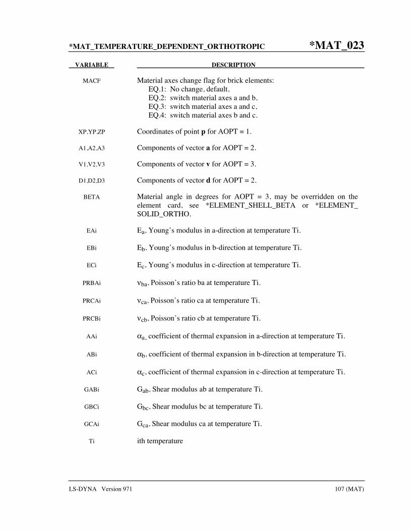
*MAT_TEMPERATURE_DEPENDENT_ORTHOTROPIC *MAT_023
LS-DYNA Version 971 107 (MAT)
VARIABLE DESCRIPTION
MACF Material axes change flag for brick elements: EQ.1: No change, default, EQ.2: switch material axes a and b, EQ.3: switch material axes a and c, EQ.4: switch material axes b and c.
XP,YP,ZP Coordinates of point p for AOPT = 1.
A1,A2,A3 Components of vector a for AOPT = 2.
V1,V2,V3 Components of vector v for AOPT = 3.
D1,D2,D3 Components of vector d for AOPT = 2.
BETA Material angle in degrees for AOPT = 3, may be overridden on the element card, see *ELEMENT_SHELL_BETA or *ELEMENT_ SOLID_ORTHO.
EAi Ea, Young’s modulus in a-direction at temperature Ti.
EBi Eb, Young’s modulus in b-direction at temperature Ti.
ECi Ec, Young’s modulus in c-direction at temperature Ti.
PRBAi νba, Poisson’s ratio ba at temperature Ti.
PRCAi νca, Poisson’s ratio ca at temperature Ti.
PRCBi νcb, Poisson’s ratio cb at temperature Ti.
AAi αa, coefficient of thermal expansion in a-direction at temperature Ti.
ABi αb, coefficient of thermal expansion in b-direction at temperature Ti.
ACi αc, coefficient of thermal expansion in c-direction at temperature Ti.
GABi Gab, Shear modulus ab at temperature Ti.
GBCi Gbc, Shear modulus bc at temperature Ti.
GCAi Gca, Shear modulus ca at temperature Ti.
Ti ith temperature

*MAT_023 *MAT_TEMPERATURE_DEPENDENT_ORTHOTROPIC
108 (MAT) LS-DYNA Version 971
Remarks:
In the implementation for three-dimensional continua a total Lagrangian formulation is used. In this approach the material law that relates second Piola-Kirchhoff stress S to the Green-St. Venant strain E is
tlS C E T C T E= ⋅ = ⋅
where T is the transformation matrix [Cook 1974].
( ) ( ) ( )( )
2 2 21 1 1 1 1 1 1 1 1
2 2 22 2 2 2 2 2 2 2 2
2 2 23 3 3 3 3 3 3 3 3
1 2 1 2 1 2 1 2 2 1 1 2 2 1 1 2 2 1
2 3 2 3 2 3 2 3 3 2
2 2 2
2 2 2
l m n l m m n n l
l m n l m m n n l
l m n l m m n n lT
l l m m n n l m l m m n m n n l n l
l l m m n n l m l m
=+ + +
+ ( ) ( )( ) ( ) ( )
2 3 3 2 2 3 3 2
3 1 3 1 3 1 3 1 1 3 3 1 1 3 3 1 1 3
2 2 2
m n m n n l n l
l l m m n n l m l m m n m n n l n l
+ +
+ + +
il , im , in are the direction cosines
1 2 3i i i ix l x m x n x′ = + + 1,2,3for i =
and ix′ denotes the material axes. The temperature dependent constitutive matrix lC is defined
in terms of the material axes as
( )( )( )
( )( )
( )( )
( )( )
( )( )
( )( ) ( )
( )
( )
( )
13 31
11 11 33
12 32
11 22 33
13 23
1 11 22 33
12
23
31
1 0 0 0
1 0 0 0
1 0 0 0
1 0 0 0 0 0
1 0 0 0 0 0
1 0 0 0 0 0
l
T T
E T E T E T
T T
E E T E T
T T
E T E T E TC
G T
G T
G T
υ υ
υ υ
υ υ−
− −
− −
− −=
where the subscripts denote the material axes, i.e.,
andi j iij x x ii xE Eυ υ ′ ′ ′= =

*MAT_TEMPERATURE_DEPENDENT_ORTHOTROPIC *MAT_023
LS-DYNA Version 971 109 (MAT)
Since lC is symmetric
12 21
11 22
,E E
υ υ= etc.
The vector of Green-St. Venant strain components is
11 22 33 12 23 31, , , , ,tE E E E E E E=
which include the local thermal strains which are integrated in time:
( )( )( )
12
12
12
1 1
1 1
1 1
nn n n naa aa a
nn n n nbb bb b
nn n n ncc cc c
T T T
T T T
T T T
ε ε α
ε ε α
ε ε α
++ +
++ +
++ +
= + −
= + −
= + −
After computing ijS we then obtain the Cauchy stress:
0
jiij kl
k l
xxS
X X
ρσρ
∂∂=∂ ∂
This model will predict realistic behavior for finite displacement and rotations as long as the strains are small.
For shell elements, the stresses are integrated in time and are updated in the corotational coordinate system. In this procedure the local material axes are assumed to remain orthogonal in the deformed configuration. This assumption is valid if the strains remain small.

*MAT_024 *MAT_PIECEWISE_LINEAR_PLASTICITY
110 (MAT) LS-DYNA Version 971
*MAT_PIECEWISE_LINEAR_PLASTICITY
This is Material Type 24. An elasto-plastic material with an arbitrary stress versus strain curve and arbitrary strain rate dependency can be defined. See also Remark below. Also, failure based on a plastic strain or a minimum time step size can be defined. For another model with a more comprehensive failure criteria see MAT_MODIFIED_PIECEWISE_LINEAR_PLASTICITY. If considering laminated or sandwich shells with non-uniform material properties (this is defined through the user specified integration rule), the model, MAT_LAYERED_LINEAR_ PLASTICITY, is recommended. If solid elements are used and if the elastic strains before yielding are finite, the model, MAT_FINITE_ELASTIC_STRAIN_PLASTICITY, treats the elastic strains using a hyperelastic formulation.
Card 1 1 2 3 4 5 6 7 8
Variable MID RO E PR SIGY ETAN FAIL TDEL
Type A8 F F F F F F F
Default none none none none none 0.0 10.E+20 0
Card 2
Variable C P LCSS LCSR VP
Type F F F F F
Default 0 0 0 0 0
Card 3
Variable EPS1 EPS2 EPS3 EPS4 EPS5 EPS6 EPS7 EPS8
Type F F F F F F F F
Default 0 0 0 0 0 0 0 0

*MAT_PIECEWISE_LINEAR_PLASTICITY *MAT_024
LS-DYNA Version 971 111 (MAT)
Card 4 1 2 3 4 5 6 7 8
Variable ES1 ES2 ES3 ES4 ES5 ES6 ES7 ES8
Type F F F F F F F F
Default 0 0 0 0 0 0 0 0
VARIABLE DESCRIPTION
MID Material identification. A unique number or label not exceeding 8 characters must be specified.
RO Mass density.
E Young’s modulus.
PR Poisson’s ratio.
SIGY Yield stress.
ETAN Tangent modulus, ignored if (LCSS.GT.0) is defined.
FAIL Failure flag. LT.0.0: User defined failure subroutine is called to determine
failure EQ.0.0: Failure is not considered. This option is recommended if
failure is not of interest since many calculations will be saved. GT.0.0: Plastic strain to failure. When the plastic strain reaches
this value, the element is deleted from the calculation.
TDEL Minimum time step size for automatic element deletion.
C Strain rate parameter, C, see formula below.
P Strain rate parameter, P, see formula below.
LCSS Load curve ID or Table ID (optional; supersedes SIGY, ETAN, EPS1-8, ES1-8). Load curve ID defining effective stress versus effective plastic strain. If defined EPS1-EPS8 and ES1-ES8 are ignored. The table ID defines for each strain rate value a load curve ID giving the stress versus effective plastic strain for that rate, See Figure 24.1. The stress versus effective plastic strain curve for the lowest value of strain rate is used if the strain rate falls below the minimum value. Likewise, the stress versus effective plastic strain curve for the highest value of strain

*MAT_024 *MAT_PIECEWISE_LINEAR_PLASTICITY
112 (MAT) LS-DYNA Version 971
VARIABLE DESCRIPTION
rate is used if the strain rate exceeds the maximum value. The strain rate parameters: C and P; the curve ID, LCSR; EPS1-EPS8 and ES1-ES8 are ignored if a Table ID is defined. NOTE: The strain rate values defined in the table may be given as the natural logarithm of the strain rate. If the first stress-strain curve in the table corresponds to a negative strain rate, LS-DYNA assumes that the natural logarithm of the strain rate value is used. Since the tables are internally discretized to equally space the points, natural logarithms are necessary, for example, if the curves correspond to rates from 10.e-04 to 10.e+04. Computing the natural logarithm of the strain rate does slow the stress update down significantly on some computers.
LCSR Load curve ID defining strain rate scaling effect on yield stress.
VP Formulation for rate effects: EQ.-1.0: Cowper-Symonds with deviatoric strain rate rather than
total. EQ.0.0: Scale yield stress (default), EQ.1.0: Viscoplastic formulation.
EPS1-EPS8 Effective plastic strain values (optional; supersedes SIGY, ETAN). At least 2 points should be defined. The first point must be zero corresponding to the initial yield stress. WARNING: If the first point is nonzero the yield stress is extrapolated to determine the initial yield. If this option is used SIGY and ETAN are ignored and may be input as zero.
ES1-ES8 Corresponding yield stress values to EPS1 - EPS8.
Remarks:
The stress strain behavior may be treated by a bilinear stress strain curve by defining the tangent modulus, ETAN. Alternately, a curve of effective stress vs. effective plastic strain similar to that shown in Figure 10.1 may be defined by (EPS1,ES1) - (EPS8,ES8); however, a curve ID (LCSS) may be referenced instead if eight points are insufficient. The cost is roughly the same for either approach. Note that in the special case of uniaxial stress, true stress vs. true plastic strain is equivalent to effective stress vs. effective plastic strain. The most general approach is to use the table definition (LCSS) discussed below.
Three options to account for strain rate effects are possible.
I. Strain rate may be accounted for using the Cowper and Symonds model which scales the yield stress with the factor
1
1p
C
ε+

*MAT_PIECEWISE_LINEAR_PLASTICITY *MAT_024
LS-DYNA Version 971 113 (MAT)
where ε is the strain rate. = ij ijε ε ε . If VP=-1. The deviatoric strain rates are used instead.
If the viscoplastic option is active, VP=1.0, and if SIGY is > 0 then the dynamic yield
stress is computed from the sum of the static stress, ( )s py effσ ε , which is typically given by a load
curve ID, and the initial yield stress, SIGY, multiplied by the Cowper-Symonds rate term as follows:
( ) ( )1
,p peffp p s p
y eff eff y eff SIGYC
εσ ε ε σ ε= + ⋅
where the plastic strain rate is used. With this latter approach similar results can be obtained between this model and material model: *MAT_ANISOTROPIC_VISCOPLASTIC. If SIGY=0,
the following equation is used instead where the static stress, ( )s py effσ ε , must be defined by a
load curve:
( ) ( )1
, 1p p
effp p s py eff eff y eff C
εσ ε ε σ ε= +
This latter equation is always used if the viscoplastic option is off.
II. For complete generality a load curve (LCSR) to scale the yield stress may be input instead. In this curve the scale factor versus strain rate is defined.
III. If different stress versus strain curves can be provided for various strain rates, the option using the reference to a table (LCSS) can be used. Then the table input in *DEFINE_TABLE has to be used, see Figure 24.1.
A fully viscoplastic formulation is optional (variable VP) which incorporates the different options above within the yield surface. An additional cost is incurred over the simple scaling but the improvement is results can be dramatic.

*MAT_024 *MAT_PIECEWISE_LINEAR_PLASTICITY
114 (MAT) LS-DYNA Version 971
Figure 24.1. Rate effects may be accounted for by defining a table of curves. If a table ID is specified a curve ID is given for each strain rate, see *DEFINE_TABLE. Intermediate values are found by interpolating between curves. Effective plastic strain versus yield stress is expected. If the strain rate values fall out of range, extrapolation is not used; rather, either the first or last curve determines the yield stress depending on whether the rate is low or high, respectively.

*MAT_GEOLOGIC_CAP_MODEL *MAT_025
LS-DYNA Version 971 115 (MAT)
*MAT_GEOLOGIC_CAP_MODEL
This is Material Type 25. This is an inviscid two invariant geologic cap model. This material model can be used for geomechanical problems or for materials as concrete, see references cited below.
Card 1 1 2 3 4 5 6 7 8
Variable MID RO BULK G ALPHA THETA GAMMA BETA
Type A8 F F F F F F F
Card 2
Variable R D W X0 C N
Type F F F F F F
Card 3
Variable PLOT FTYPE VEC TOFF
Type F F F F
VARIABLE DESCRIPTION
MID Material identification. A unique number or label not exceeding 8 characters must be specified.
RO Mass density.
BULK Initial bulk modulus, K.
G Initial Shear modulus.
ALPHA Failure envelope parameter, α.
THETA Failure envelope linear coefficient, θ.
GAMMA Failure envelope exponential coefficient, γ.

*MAT_025 *MAT_GEOLOGIC_CAP_MODEL
116 (MAT) LS-DYNA Version 971
VARIABLE DESCRIPTION
BETA Failure envelope exponent, β.
R Cap, surface axis ratio.
D Hardening law exponent.
W Hardening law coefficient.
X0 Hardening law exponent, X0.
C Kinematic hardening coefficient, c .
N Kinematic hardening parameter.
PLOT Save the following variable for plotting in LS-Prepost, to be labeled there as “effective plastic strain:”
EQ.1: hardening parameter, κ, EQ.2: cap -J1 axis intercept, X (κ),
EQ.3: volumetric plastic strain pvε ,
EQ.4: first stress invariant, J1,
EQ.5: second stress invariant, J2 EQ.6: not used EQ.7: not used EQ.8: response mode number EQ.9: number of iterations.
FTYPE Formulation flag: EQ.1: soil or concrete (Cap surface may contract),
EQ.2: rock (Cap doesn’t contract).
VEC Vectorization flag: EQ.0: vectorized (fixed number of iterations),
EQ.1: fully iterative, If the vectorized solution is chosen, the stresses might be slightly off
the yield surface; however, on vector computers a much more efficient solution is achieved.
TOFF Tension Cut Off, TOFF < 0 (positive in compression).
Remarks:
The implementation of an extended two invariant cap model, suggested by Stojko [1990], is based on the formulations of Simo, et al. [1988, 1990] and Sandler and Rubin [1979]. In this model, the two invariant cap theory is extended to include nonlinear kinematic hardening as suggested by Isenberg, Vaughan, and Sandler [1978]. A brief discussion of the extended cap model and its parameters is given below.

*MAT_GEOLOGIC_CAP_MODEL *MAT_025
LS-DYNA Version 971 117 (MAT)
Figure 25.1. The yield surface of the two-invariant cap model in pressure 2 1DJ J− space.
Surface f1 is the failure envelope, f2 is the cap surface, and f3 is the tension cutoff.
The cap model is formulated in terms of the invariants of the stress tensor. The square
root of the second invariant of the deviatoric stress tensor, 2DJ is found from the deviatoric
stresses s as
2
1
2D ij ijJ S S≡
and is the objective scalar measure of the distortional or shearing stress. The first invariant of the stress, J1, is the trace of the stress tensor.
The cap model consists of three surfaces in 2 1DJ J− space, as shown in Figure 25.1.
First, there is a failure envelope surface, denoted f1 in the figure. The functional form of f1 is
( )( )1 2 1min ,D e misesf J F J T= − ,
where Fe is given by
( ) ( )1 1 1expeF J J Jα γ β θ≡ − − +
and ( ) ( )mises n nT X Lκ κ≡ − . This failure envelop surface is fixed in 2 1DJ J− space, and
therefore does not harden unless kinematic hardening is present. Next, there is a cap surface, denoted f2 in the figure, with f2 given by
( )2 2 1,D cf J F J K= −

*MAT_025 *MAT_GEOLOGIC_CAP_MODEL
118 (MAT) LS-DYNA Version 971
where Fc is defined by
( ) ( ) ( ) ( )2 2
1 1
1,cF J X L J L
Rκ κ κ κ≡ − − − ,
( )X κ is the intersection of the cap surface with the J1 axis
( ) ( )eX RFκ κ κ= + ,
and ( )L κ is defined by
( ) if > 0
0 if 0L
κ κκ
κ≡
≤
The hardening parameter κ is related to the plastic volume change pvε through the hardening law
( )( ){ }01 exppv W D X Xε κ= − − −
Geometrically, κ is seen in the figure as the J1 coordinate of the intersection of the cap surface and the failure surface. Finally, there is the tension cutoff surface, denoted f3 in the figure. The function f3 is given by
3 1f T-J≡
where T is the input material parameter which specifies the maximum hydrostatic tension
sustainable by the material. The elastic domain in 2 1DJ J− space is then bounded by the
failure envelope surface above, the tension cutoff surface on the left, and the cap surface on the right.
An additive decomposition of the strain into elastic and plastic parts is assumed:
ε = εe + εp,
where εe is the elastic strain and εp is the plastic strain. Stress is found from the elastic strain using Hooke’s law,
σ = C(ε - εp),
where σ is the stress and C is the elastic constitutive tensor.
The yield condition may be written

*MAT_GEOLOGIC_CAP_MODEL *MAT_025
LS-DYNA Version 971 119 (MAT)
( )( )( )
1
2
3
0
, 0
0
f s
f s
f s
κ≤
≤
≤
and the plastic consistency condition requires that
0
1,2,3
0
k k
k
f
k
λ
λ
==
≥
where kλ is the plastic consistency parameter for surface k. If 0kf < then, 0kλ = and the
response is elastic. If 0kf > then surface k is active and kλ is found from the requirement that
0kf = .
Associated plastic flow is assumed, so using Koiter’s flow rule the plastic strain rate is given as the sum of contribution from all of the active surfaces,
3
1
p kk
k
f
sε λ
=
∂=∂
.
One of the major advantages of the cap model over other classical pressure-dependent plasticity models is the ability to control the amount of dilatancy produced under shear loading. Dilatancy is produced under shear loading as a result of the yield surface having a positive slope in
2DJ J− space, so the assumption of plastic flow in the direction normal to the yield surface
produces a plastic strain rate vector that has a component in the volumetric (hydrostatic) direction (see Figure 25.1). In models such as the Drucker-Prager and Mohr-Coulomb, this dilatancy continues as long as shear loads are applied, and in many cases produces far more dilatancy than is experimentally observed in material tests. In the cap model, when the failure surface is active, dilatancy is produced just as with the Drucker-Prager and Mohr-Coulumb models. However, the hardening law permits the cap surface to contract until the cap intersects the failure envelope at the stress point, and the cap remains at that point. The local normal to the yield surface is now vertical, and therefore the normality rule assures that no further plastic volumetric strain (dilatancy) is created. Adjustment of the parameters that control the rate of cap contractions permits experimentally observed amounts of dilatancy to be incorporated into the cap model, thus producing a constitutive law which better represents the physics to be modeled.
Another advantage of the cap model over other models such as the Drucker-Prager and Mohr-Coulomb is the ability to model plastic compaction. In these models all purely volumetric response is elastic. In the cap model, volumetric response is elastic until the stress point hits the cap surface. Therefore, plastic volumetric strain (compaction) is generated at a rate controlled by the hardening law. Thus, in addition to controlling the amount of dilatancy, the introduction of the cap surface adds another experimentally observed response characteristic of geological material into the model.

*MAT_025 *MAT_GEOLOGIC_CAP_MODEL
120 (MAT) LS-DYNA Version 971
The inclusion of kinematic hardening results in hysteretic energy dissipation under cyclic loading conditions. Following the approach of Isenberg, et al. [1978] a nonlinear kinematic hardening law is used for the failure envelope surface when nonzero values of and N are specified. In this case, the failure envelope surface is replaced by a family of yield surfaces bounded by an initial yield surface and a limiting failure envelope surface. Thus, the shape of the yield surfaces described above remains unchanged, but they may translate in a plane orthogonal to the J axis,
Translation of the yield surfaces is permitted through the introduction of a “back stress” tensor, α The formulation including kinematic hardening is obtained by replacing the stress σwith the translated stress tensor η σ α≡ − in all of the above equation. The history tensor α is assumed deviatoric, and therefore has only 5 unique components. The evolution of the back stress tensor is governed by the nonlinear hardening law
( ), pcF eα σ α=
where c is a constant, F is a scalar function of σ and α and pe is the rate of deviatoric plastic strain. The constant may be estimated from the slope of the shear stress - plastic shear strain curve at low levels of shear stress.
The function F is defined as
( )( )1
max 0,12 e
FNF J
σ α α− •≡ −
where N is a constant defining the size of the yield surface. The value of N may be interpreted as the radial distant between the outside of the initial yield surface and the inside of the limit surface. In order for the limit surface of the kinematic hardening cap model to correspond with the failure envelope surface of the standard cap model, the scalar parameter a must be replaced α - N in the definition Fe.
The cap model contains a number of parameters which must be chosen to represent a particular material, and are generally based on experimental data. The parameters α, β, θ, and γare usually evaluated by fitting a curve through failure data taken from a set of triaxial compression tests. The parameters W, D, and X0 define the cap hardening law. The value W represents the void fraction of the uncompressed sample and D governs the slope of the initial loading curve in hydrostatic compression. The value of R is the ration of major to minor axes of the quarter ellipse defining the cap surface. Additional details and guidelines for fitting the cap model to experimental data are found in Chen and Baladi [1985].

*MAT_HONEYCOMB *MAT_026
LS-DYNA Version 971 121 (MAT)
*MAT_HONEYCOMB
This is Material Type 26. The major use of this material model is for honeycomb and foam materials with real anisotropic behavior. A nonlinear elastoplastic material behavior can be defined separately for all normal and shear stresses. These are considered to be fully uncoupled. See notes below.
Card 1 1 2 3 4 5 6 7 8
Variable MID RO E PR SIGY VF MU BULK
Type A8 F F F F F F F
Default none none none none none none .05 0.0
Card 2
Variable LCA LCB LCC LCS LCAB LCBC LCCA LCSR
Type F F F F F F F F
Default none LCA LCA LCA LCS LCS LCS optional
Card 3
Variable EAAU EBBU ECCU GABU GBCU GCAU AOPT MACF
Type F F F F F F I
Card 4
Variable XP YP ZP A1 A2 A3
Type F F F F F F

*MAT_026 *MAT_HONEYCOMB
122 (MAT) LS-DYNA Version 971
Card 5 1 2 3 4 5 6 7 8
Variable D1 D2 D3 TSEF SSEF
Type F F F F F
VARIABLE DESCRIPTION
MID Material identification. A unique number or label not exceeding 8 characters must be specified.
RO Mass density.
E Young’s modulus for compacted honeycomb material.
PR Poisson’s ratio for compacted honeycomb material.
SIGY Yield stress for fully compacted honeycomb.
VF Relative volume at which the honeycomb is fully compacted.
MU μ, material viscosity coefficient. (default=.05) Recommended.
BULK Bulk viscosity flag: EQ.0.0: bulk viscosity is not used. This is recommended. EQ.1.0: bulk viscosity is active and μ=0. This will give results
identical to previous versions of LS-DYNA.
LCA Load curve ID, see *DEFINE_CURVE, for sigma-aa versus either relative volume or volumetric strain. See notes below.
LCB Load curve ID, see *DEFINE_CURVE, for sigma-bb versus either relative volume or volumetric strain. Default LCB=LCA. See notes below.
LCC Load curve ID, see *DEFINE_CURVE, for sigma-cc versus either relative volume or volumetric strain. Default LCC=LCA. See notes below.
LCS Load curve ID, see *DEFINE_CURVE, for shear stress versus either relative volume or volumetric strain. Default LCS=LCA. Each component of shear stress may have its own load curve. See notes below.

*MAT_HONEYCOMB *MAT_026
LS-DYNA Version 971 123 (MAT)
VARIABLE DESCRIPTION
LCAB Load curve ID, see *DEFINE_CURVE, for sigma-ab versus either relative volume or volumetric strain. Default LCAB=LCS. See notes below.
LCBC Load curve ID, see *DEFINE_CURVE, for sigma-bc versus either relative volume or volumetric strain. Default LCBC=LCS. See notes below.
LCCA Load curve ID, see *DEFINE_CURVE, or sigma-ca versus either relative volume or volumetric strain. Default LCCA=LCS. See notes below.
LCSR Load curve ID, see *DEFINE_CURVE, for strain-rate effects defining the scale factor versus strain rate. This is optional. The curves defined above are scaled using this curve.
EAAU Elastic modulus Eaau in uncompressed configuration.
EBBU Elastic modulus Ebbu in uncompressed configuration.
ECCU Elastic modulus Eccu in uncompressed configuration.
GABU Shear modulus Gabu in uncompressed configuration.
GBCU Shear modulus Gbcu in uncompressed configuration.
GCAU Shear modulus Gcau in uncompressed configuration.
AOPT Material axes option (see MAT_OPTION TROPIC_ELASTIC for a more complete description):
EQ.0.0: locally orthotropic with material axes determined by element nodes 1, 2, and 4, as with *DEFINE_COORDINATE_ NODES.
EQ.1.0: locally orthotropic with material axes determined by a point in space and the global location of the element center; this is the a-direction.
EQ.2.0: globally orthotropic with material axes determined by vectors defined below, as with *DEFINE_COORDINATE_ VECTOR.
LT.0.0: the absolute value of AOPT is a coordinate system ID number (CID on *DEFINE_COORDINATE_NODES, *DEFINE_ COORDINATE_SYSTEM or *DEFINE_COORDINATE_ VECTOR). Available in R3 version of 971 and later.

*MAT_026 *MAT_HONEYCOMB
124 (MAT) LS-DYNA Version 971
VARIABLE DESCRIPTION
MACF Material axes change flag: EQ.1: No change, default, EQ.2: switch material axes a and b, EQ.3: switch material axes a and c, EQ.4: switch material axes b and c.
XP YP ZP Coordinates of point p for AOPT = 1.
A1 A2 A3 Components of vector a for AOPT = 2.
D1 D2 D3 Components of vector d for AOPT = 2.
TSEF Tensile strain at element failure (element will erode).
SSEF Shear strain at element failure (element will erode).
Remarks:
For efficiency it is strongly recommended that the load curve ID’s: LCA, LCB, LCC, LCS, LCAB, LCBC, and LCCA, contain exactly the same number of points with corresponding strain values on the abscissa. If this recommendation is followed the cost of the table lookup is insignificant. Conversely, the cost increases significantly if the abscissa strain values are not consistent between load curves.
The behavior before compaction is orthotropic where the components of the stress tensor are uncoupled, i.e., an a component of strain will generate resistance in the local a-direction with no coupling to the local b and c directions. The elastic moduli vary, from their initial values to the fully compacted values at Vf, linearly with the relative volume V:
( )
( )
( )
( )
( )
( )
aa aau aau
bb bbu bbu
cc ccu ccu
ab abu abu
bc bcu bcu
ca cau cau
E E E E
E E E E
E E E E
G E G G
G E G G
G E G G
β
β
β
β
β
β
= + −
= + −
= + −
= + −
= + −
= + −
where

*MAT_HONEYCOMB *MAT_026
LS-DYNA Version 971 125 (MAT)
1max min ,1 ,0
1 f
V
Vβ −=
−
and G is the elastic shear modulus for the fully compacted honeycomb material
( )2 1
EG
v=
+.
The relative volume, V, is defined as the ratio of the current volume to the initial volume. Typically, V=1 at the beginning of a calculation. The viscosity coefficient μ (MU) should be set to a small number (usually .02-.10 is okay). Alternatively, the two bulk viscosity coefficients on the control cards should be set to very small numbers to prevent the development of spurious pressures that may lead to undesirable and confusing results. The latter is not recommended since spurious numerical noise may develop.
The load curves define the magnitude of the average stress as the material changes density (relative volume), see Figure 26.1. Each curve related to this model must have the same number of points and the same abscissa values. There are two ways to define these curves, a) asa function of relative volume (V) or b) as a function of volumetric strain defined as:
1V Vε = −
In the former, the first value in the curve should correspond to a value of relative volume slightly less than the fully compacted value. In the latter, the first value in the curve should be less than or equal to zero, corresponding to tension, and increase to full compaction. Care should be taken when defining the curves so that extrapolated values do not lead to negative yield stresses.
At the beginning of the stress update each element’s stresses and strain rates are transformed into the local element coordinate system. For the uncompacted material, the trial stress components are updated using the elastic interpolated moduli according to:
1
1
1
1
1
1
2
2
2
trial
trial
trial
trial
trial
trial
n naa aa aa aa
n nbb bb bb bb
n ncc cc cc cc
n nab ab ab ab
n nbc bc bc bc
n nca ca ca ca
E
E
E
G
G
G
σ σ ε
σ σ ε
σ σ ε
σ σ ε
σ σ ε
σ σ ε
+
+
+
+
+
+
= + Δ
= + Δ
= + Δ
= + Δ
= + Δ
= + Δ

*MAT_026 *MAT_HONEYCOMB
126 (MAT) LS-DYNA Version 971
Each component of the updated stresses is then independently checked to ensure that they do not exceed the permissible values determined from the load curves; e.g., if
( )1trialnij ij Vσ λσ+ >
then
( )1
1
1
trial
trial
nijn
ij ij nij
Vλσ
σ σλσ
++
+=
On Card 2 σij (V) is defined by LCA for the aa stress component, LCB for the bb component, LCC for the cc component, and LCS for the ab, bc, ca shear stress components. The parameter λis either unity or a value taken from the load curve number, LCSR, that defines λ as a function of strain-rate. Strain-rate is defined here as the Euclidean norm of the deviatoric strain-rate tensor.
For fully compacted material it is assumed that the material behavior is elastic-perfectly plastic and the stress components updated according to:
12
2n
trial n devij ij ijs s G ε
+
= + Δ
where the deviatoric strain increment is defined as
1
3devij ij kk ijε ε ε δΔ = Δ − Δ
Now a check is made to see if the yield stress for the fully compacted material is exceeded by comparing
( ) 123
2trial trial trialeff ij ijs s s=
the effective trial stress to the defined yield stress, SIGY. If the effective trial stress exceeds the yield stress the stress components are simply scaled back to the yield surface
1 yn trialij ijtrial
eff
s ss
σ+ = .
Now the pressure is updated using the elastic bulk modulus, K
( )
11 2
3 1 2
nn nkkp p K
EK
v
ε ++ = − Δ
=−
to obtain the final value for the Cauchy stress

*MAT_HONEYCOMB *MAT_026
LS-DYNA Version 971 127 (MAT)
1 1 1n n nij ij ijs pσ δ+ + += −
After completing the stress update transform the stresses back to the global configuration.
Figure 26.1. Stress quantity versus volumetric strain. Note that the “yield stress” at a volumetric strain of zero is non-zero. In the load curve definition, see *DEFINE_CURVE, the “time” value is the volumetric strain and the “function” value is the yield stress.

*MAT_027 *MAT_MOONEY-RIVLIN_RUBBER
128 (MAT) LS-DYNA Version 971
*MAT_MOONEY-RIVLIN_RUBBER
This is Material Type 27. A two-parametric material model for rubber can be defined.
Card 1 1 2 3 4 5 6 7 8
Variable MID RO PR A B REF
Type A8 F F F F F
Card 2
Variable SGL SW ST LCID
Type F F F F
VARIABLE DESCRIPTION
MID Material identification. A unique number or label not exceeding 8 characters must be specified.
RO Mass density.
PR Poisson’s ratio (value between 0.49 and 0.5 is recommended, smaller values may not work).
A Constant, see literature and equations defined below.
B Constant, see literature and equations defined below.
REF Use reference geometry to initialize the stress tensor. The reference geometry is defined by the keyword:*INITIAL_FOAM_REFERENCE_ GEOMETRY (see there for more details).
EQ.0.0: off, EQ.1.0: on.
If A=B=0.0, then a least square fit is computed from tabulated uniaxial data via a load curve. The following information should be defined.
SGL Specimen gauge length l0, see Figure 27.1.

*MAT_MOONEY-RIVLIN_RUBBER *MAT_027
LS-DYNA Version 971 129 (MAT)
VARIABLE DESCRIPTION
SW Specimen width, see Figure 27.1.
ST Specimen thickness, see Figure 27.1.
LCID Load curve ID, see *DEFINE_CURVE, giving the force versus actual change ΔL in the gauge length. See also Figure 27.2 for an alternative definition.
Remarks:
The strain energy density function is defined as:
( ) ( ) ( ) ( )223 3 1 1W A I B II C III D III−= − + − + − + −
where
C = 0.5 A + B
( ) ( )( )
5 2 11 5
2 1 2
A BD
υ υυ
− + −=
−
υ =Poisson’s ratio
2(A+B) = shear modulus of linear elasticity
I, II, III = invariants of right Cauchy-Green Tensor C.
The load curve definition that provides the uniaxial data should give the change in gauge length, ΔL, versus the corresponding force. In compression both the force and the change in gauge length must be specified as negative values. In tension the force and change in gauge length should be input as positive values. The principal stretch ratio in the uniaxial direction, λ1,is then given by
01
0
L L
Lλ + Δ=
with L0 being the initial length and L being the actual length.
Alternatively, the stress versus strain curve can also be input by setting the gauge length, thickness, and width to unity (1.0) and defining the engineering strain in place of the change in gauge length and the nominal (engineering) stress in place of the force, see Figure 27.2.
The least square fit to the experimental data is performed during the initialization phase and is a comparison between the fit and the actual input is provided in the d3hsp file. It is a good idea to visually check to make sure it is acceptable. The coefficients A and B are also printed in

*MAT_027 *MAT_MOONEY-RIVLIN_RUBBER
130 (MAT) LS-DYNA Version 971
the output file. It is also advised to use the material driver (see Appendix K) for checking out the material model.
Figure 27.1. Uniaxial specimen for experimental data.
Figure 27.2. The stress versus strain curve can used instead of the force versus the change in the gauge length by setting the gauge length, thickness, and width to unity (1.0) and defining the engineering strain in place of the change in gauge length and the nominal (engineering) stress in place of the force. *MAT_077_O is a better alternative for fitting data resembling the curve above. *MAT_027 will provide a poor fit to a curve that exhibits an strong upturn in slope as strains become large.

*MAT_RESULTANT_PLASTICITY *MAT_028
LS-DYNA Version 971 131 (MAT)
*MAT_RESULTANT_PLASTICITY
This is Material Type 28. A resultant formulation for beam and shell elements including elasto-plastic behavior can be defined. This model is available for the Belytschko-Schwer beam, the Co
triangular shell, the Belytschko-Tsay shell, and the fully integrated type 16 shell. For beams, the treatment is elastic-perfectly plastic, but for shell elements isotropic hardening is approximately modeled. For a detailed description we refer to the LS-DYNA Theory Manual. Since the stresses are not computed in the resultant formulation, the stresses output to the binary databases for the resultant elements are zero.
Card 1 1 2 3 4 5 6 7 8
Variable MID RO E PR SIGY ETAN
Type A8 F F F F F
Default none none none none none 0.0
VARIABLE DESCRIPTION
MID Material identification. A unique number or label not exceeding 8 characters must be specified.
RO Mass density
E Young’s modulus
PR Poisson’s ratio
SIGY Yield stress
ETAN Plastic hardening modulus (for shells only)

*MAT_029 *MAT_FORCE_LIMITED
132 (MAT) LS-DYNA Version 971
*MAT_FORCE_LIMITED
This is Material Type 29. With this material model, for the Belytschko-Schwer beam only, plastic hinge forming at the ends of a beam can be modeled using curve definitions. Optionally, collapse can also be modeled. See also *MAT_139.
Description: FORCE LIMITED Resultant Formulation
Card 1 1 2 3 4 5 6 7 8
Variable MID RO E PR DF AOPT YTFLAG ASOFT
Type A8 F F F F F F F
Default none none none none 0.0 0.0 0.0 0.0
Card 2
Variable M1 M2 M3 M4 M5 M6 M7 M8
Type F F F F F F F F
Default none 0 0 0 0 0 0 0
Card 3
Variable LC1 LC2 LC3 LC4 LC5 LC6 LC7 LC8
Type F F F F F F F F
Default none 0 0 0 0 0 0 0

*MAT_FORCE_LIMITED *MAT_029
LS-DYNA Version 971 133 (MAT)
Card 4 1 2 3 4 5 6 7 8
Variable LPS1 SFS1 LPS2 SFS2 YMS1 YMS2
Type F F F F F F
Default 0 1.0 LPS1 1.0 1.0E+20 YMS1
Card 5
Variable LPT1 SFT1 LPT2 SFT2 YMT1 YMT2
Type F F F F F F
Default 0 1.0 LPT1 1.0 1.0E+20 YMT1
Card 6
Variable LPR SFR YMR
Type F F F
Default 0 1.0 1.0E+20
VARIABLE DESCRIPTION
MID Material identification. A unique number or label not exceeding 8 characters must be specified.
RO Mass density
E Young’s modulus
PR Poisson’s ratio
DF Damping factor, see definition in notes below. A proper control for the timestep has to be maintained by the user!

*MAT_029 *MAT_FORCE_LIMITED
134 (MAT) LS-DYNA Version 971
VARIABLE DESCRIPTION
AOPT Axial load curve option: EQ.0.0: axial load curves are force versus strain, EQ.1.0: axial load curves are force versus change in length. LT.0.0: the absolute value of AOPT is a coordinate system ID
number (CID on *DEFINE_COORDINATE_NODES, *DEFINE_ COORDINATE_SYSTEM or *DEFINE_COORDINATE_ VECTOR). Available in R3 version of 971 and later.
YTFLAG Flag to allow beam to yield in tension: EQ.0.0: beam does not yield in tension, EQ.1.0: beam can yield in tension.
ASOFT Axial elastic softening factor applied once hinge has formed. When a hinge has formed the stiffness is reduced by this factor. If zero, this factor is ignored.
M1, M2,...,M8 Applied end moment for force versus (strain/change in length) curve. At least one must be defined. A maximum of 8 moments can be defined. The values should be in ascending order.
LC1, LC2,...,LC8 Load curve ID (see *DEFINE_CURVE) defining axial force (collapse load) versus strain/change in length (see AOPT) for the corresponding applied end moment. Define the same number as end moments. Each curve must contain the same number of points.
LPS1 Load curve ID for plastic moment versus rotation about s-axis at node 1. If zero, this load curve is ignored.
SFS1 Scale factor for plastic moment versus rotation curve about s-axis at node 1. Default = 1.0.
LPS2 Load curve ID for plastic moment versus rotation about s-axis at node 2. Default: is same as at node 1.
SFS2 Scale factor for plastic moment versus rotation curve about s-axis at node 2. Default: is same as at node 1.
YMS1 Yield moment about s-axis at node 1 for interaction calculations (default set to 1.0E+20 to prevent interaction).
YMS2 Yield moment about s-axis at node 2 for interaction calculations (default set to YMS1).
LPT1 Load curve ID for plastic moment versus rotation about t-axis at node 1. If zero, this load curve is ignored.

*MAT_FORCE_LIMITED *MAT_029
LS-DYNA Version 971 135 (MAT)
VARIABLE DESCRIPTION
SFT1 Scale factor for plastic moment versus rotation curve about t-axis at node 1. Default = 1.0.
LPT2 Load curve ID for plastic moment versus rotation about t-axis at node 2.Default: is the same as at node 1.
SFT2 Scale factor for plastic moment versus rotation curve about t-axis at node 2. Default: is the same as at node 1.
YMT1 Yield moment about t-axis at node 1 for interaction calculations (default set to 1.0E+20 to prevent interactions)
YMT2 Yield moment about t-axis at node 2 for interaction calculations (default set to YMT1)
LPR Load curve ID for plastic torsional moment versus rotation. If zero, this load curve is ignored.
SFR Scale factor for plastic torsional moment versus rotation (default = 1.0).
YMR Torsional yield moment for interaction calculations (default set to 1.0E+20 to prevent interaction)
Remarks:
This material model is available for the Belytschko resultant beam element only. Plastic hinges form at the ends of the beam when the moment reaches the plastic moment. The moment versus rotation relationship is specified by the user in the form of a load curve and scale factor. The points of the load curve are (plastic rotation in radians, plastic moment). Both quantities should be positive for all points, with the first point being (zero, initial plastic moment). Within this constraint any form of characteristic may be used, including flat or falling curves. Different load curves and scale factors may be specified at each node and about each of the local s and t axes. Axial collapse occurs when the compressive axial load reaches the collapse load. Collapse load versus collapse deflection is specified in the form of a load curve. The points of the load curve are either (true strain, collapse force) or (change in length, collapse force). Both quantities should be entered as positive for all points, and will be interpreted as compressive. The first point should be (zero, initial collapse load). The collapse load may vary with end moment as well as with deflections. In this case several load-deflection curves are defined, each corresponding to a different end moment. Each load curve should have the same number of points and the same deflection values. The end moment is defined as the average of the absolute moments at each end of the beam and is always positive. Stiffness-proportional damping may be added using the damping factor λ. This is defined as follows:
2 ξλω∗=

*MAT_029 *MAT_FORCE_LIMITED
136 (MAT) LS-DYNA Version 971
where ξ is the damping factor at the reference frequency ω (in radians per second). For example if 1% damping at 2Hz is required
2 0.010.001592
2 2λ
π∗= =
∗If damping is used, a small timestep may be required. LS-DYNA does not check this so to avoid instability it may be necessary to control the timestep via a load curve. As a guide, the timestep required for any given element is multiplied by 0.3L⁄cλ when damping is present (L = element length, c = sound speed).
Moment Interaction: Plastic hinges can form due to the combined action of moments about the three axes. This facility is activated only when yield moments are defined in the material input. A hinge forms when the following condition is first satisfied.
2 2 2
1r s t
ryield syield tyield
M M M
M M M+ + ≥
where,
Mr, Ms, Mt = current moment
Mryield, Msyield, Mtyield = yield moment
Note that scale factors for hinge behavior defined in the input will also be applied to the yield moments: for example, Msyield in the above formula is given by the input yield moment about the local axis times the input scale factor for the local s axis. For strain-softening characteristics, the yield moment should generally be set equal to the initial peak of the moment-rotation load curve. On forming a hinge, upper limit moments are set. These are given by
,2
yield
upper
r
r r
MM MAX M=
and similar for Ms and Mt. Thereafter the plastic moments will be given by
Mrp, = min (Mrupper, Mrcurve) and similar for s and t
where
Mrp = current plastic moment
Mrcurve = moment taken from load curve at the current rotation scaled according to the scale factor.
The effect of this is to provide an upper limit to the moment that can be generated; it represents the softening effect of local buckling at a hinge site. Thus if a member is bent about is local s-axis it will then be weaker in torsion and about its local t-axis. For moments-softening curves,

*MAT_FORCE_LIMITED *MAT_029
LS-DYNA Version 971 137 (MAT)
the effect is to trim off the initial peak (although if the curves subsequently harden, the final hardening will also be trimmed off). It is not possible to make the plastic moment vary with axial load.
axial force
strains or change in length (see AOPT)
M1
2
4
8M
M
M
M
M
M
M
3
5
6
7
Figure 29.1. The force magnitude is limited by the applied end moment. For an intermediate value of the end moment LS-DYNA interpolates between the curves to determine the allowable force value.

*MAT_030 *MAT_SHAPE_MEMORY
138 (MAT) LS-DYNA Version 971
*MAT_SHAPE_MEMORY
This is material type 30. This material model describes the superelastic response present in shape-memory alloys (SMA), that is the peculiar material ability to undergo large deformations with a full recovery in loading-unloading cycles (See Figure 30.1). The material response is always characterized by a hysteresis loop. See the references by Auricchio, Taylor and Lubliner [1997] and Auricchio and Taylor [1997]. This model is available for shell and solid elements. For Hughes-Liu beam elements it is available starting in Release 3 of version 971.
Card 1 1 2 3 4 5 6 7 8
Variable MID RO E PR
Type A8 F F F
Default none none none none
Card 2
Variable SIG_ASS SIG_ASF SIG_SAS SIG_SAF EPSL ALPHA YMRT
Type F F F F F F F
Default none none none none none 0.0 0.0
VARIABLE DESCRIPTION
MID Material identification. A unique number or label not exceeding 8 characters must be specified.
RO Density
E Young’s modulus
PR Poisson’s ratio
SIG_ASS Starting value for the forward phase transformation (conversion of austenite into martensite) in the case of a uniaxial tensile state of stress. A load curve for SIG_ASS as a function of temperature is specified by using the negative of the load curve ID number.

*MAT_SHAPE_MEMORY *MAT_030
LS-DYNA Version 971 139 (MAT)
VARIABLE DESCRIPTION
SIG_ASF Final value for the forward phase transformation (conversion of austenite into martensite) in the case of a uniaxial tensile state of stress. SIG_ASF as a function of temperature is specified by using the negative of the load curve ID number.
SIG_SAS Starting value for the reverse phase transformation (conversion of martensite into austenite) in the case of a uniaxial tensile state of stress. SIG_SAS as a function of temperature is specified by using the negative of the load curve ID number.
SIG_SAF Final value for the reverse phase transformation (conversion of martensite into austenite) in the case of a uniaxial tensile state of stress. SIG_SAF as a function of temperature is specified by using the negative of the load curve ID number.
EPSL Recoverable strain or maximum residual strain. It is a measure of the maximum deformation obtainable all the martensite in one direction.
ALPHA Parameter measuring the difference between material responses in tension and compression (set alpha = 0 for no difference). Also, see the following Remark.
YMRT Young’s modulus for the martensite if it is different from the modulus for the austenite. Defaults to the austenite modulus if it is set to zero.
Remarks:
The material parameter alpha, α, measures the difference between material responses in tension and compression. In particular, it is possible to relate the parameter α to the initial stress value of the austenite into martensite conversion, indicated respectively as ,AS
sσ + and ,ASsσ − ,
according to the following expression:
, ,
, ,
AS ASs sAS ASs s
σ σασ σ
− +
− +−=+

*MAT_030 *MAT_SHAPE_MEMORY
140 (MAT) LS-DYNA Version 971
Figure 30.1. Pictorial representation of superelastic behavior for a shape-memory material.
In the following, the results obtained from a simple test problem is reported. The material properties are set as:
E 60000 MPa
Nu 0.3
sig_AS_s 520 MPa
sig_AS_f 600 MPa
sig_SA_s 300 MPa
sig_SA_f 200 MPa
epsL 0.07
alpha 0.12
ymrt 50000 MPa
ASf
SAf
ASs
Lε
SAs

*MAT_SHAPE_MEMORY *MAT_030
LS-DYNA Version 971 141 (MAT)
The investigated problem is the complete loading-unloading test in tension and compression. The uniaxial Cauchy stress versus the logarithmic strain is plotted in Figure 30.2.
Figure 30.2. Complete loading-unloading test in tension and compression

*MAT_031 *MAT_FRAZER_NASH_RUBBER_MODEL
142 (MAT) LS-DYNA Version 971
*MAT_FRAZER_NASH_RUBBER_MODEL
This is Material Type 31. This model defines rubber from uniaxial test data. It is a modified form of the hyperelastic constitutive law first described in Kenchington [1988]. See also the notes below.
Card 1 1 2 3 4 5 6 7 8
Variable MID RO PR C100 C200 C300 C400
Type A8 F F F F F F
Card 2
Variable C110 C210 C010 C020 EXIT EMAX EMIN REF
Type F F F F F F F F
Card 3
Variable SGL SW ST LCID
Type F F F F
VARIABLE DESCRIPTION
MID Material identification. A unique number or label not exceeding 8 characters must be specified.
RO Mass density.
PR Poisson’s ratio. Values between .49 and .50 are suggested.
C100 C100 (EQ.1.0 if term is in the least squares fit.)
C200 C200 (EQ.1.0 if term is in the least squares fit.)
C300 C300 (EQ.1.0 if term is in the least squares fit.)
C400 C400 (EQ.1.0 if term is in the least squares fit.)

*MAT_FRAZER_NASH_RUBBER_MODEL *MAT_031
LS-DYNA Version 971 143 (MAT)
VARIABLE DESCRIPTION
C110 C110 (EQ.1.0 if term is in the least squares fit.)
C210 C210 (EQ.1.0 if term is in the least squares fit.)
C010 C010 (EQ.1.0 if term is in the least squares fit.)
C020 C020 (EQ.1.0 if term is in the least squares fit.)
EXIT Exit option: EQ. 0.0: stop if strain limits are exceeded (recommended), NE. 0.0: continue if strain limits are exceeded. The curve is then
extrapolated.
EMAX Maximum strain limit, (Green-St, Venant Strain).
EMIN Minimum strain limit, (Green-St, Venant Strain).
REF Use reference geometry to initialize the stress tensor. The reference geometry is defined by the keyword: *INITIAL_FOAM_ REFERENCE_GEOMETRY (see there for more details).
EQ.0.0: off, EQ.1.0: on.
SGL Specimen gauge length, see Figure 27.1.
SW Specimen width, see Figure 27.1.
ST Specimen thickness, see Figure 27.1.
LCID Load curve ID, see DEFINE_CURVE, giving the force versus actual change in gauge length. See also Figure 27.2 for an alternative definition.
Remarks:
The constants can be defined directly or a least squares fit can be performed if the uniaxial data (SGL, SW, ST and LCID) is available. If a least squares fit is chosen, then the terms to be included in the energy functional are flagged by setting their corresponding coefficients to unity. If all coefficients are zero the default is to use only the terms involving I1and I2. C100 defaults to unity if the least square fit is used.
The strain energy functional, U, is defined in terms of the input constants as:
( )
2 3 4100 1 200 1 300 1 400 1 110 1 2
2 2210 1 2 010 2 020 2
U C I C I C I C I C I I
C I I C I C I f J
= + + + + +
+ + +

*MAT_031 *MAT_FRAZER_NASH_RUBBER_MODEL
144 (MAT) LS-DYNA Version 971
where the invariants can be expressed in terms of the deformation gradient matrix, Fij, and the Green-St. Venant strain tensor, Eij :
1
2
1
2!
ij
ii
ijpq pi qj
J F
I E
I E Eδ
=
=
=
The derivative of U with respect to a component of strain gives the corresponding component of stress
ijij
US
E
∂=∂
here, Sij, is the second Piola-Kirchhoff stress tensor.
The load curve definition that provides the uniaxial data should give the change in gauge length, ΔL, and the corresponding force. In compression both the force and the change in gauge length must be specified as negative values. In tension the force and change in gauge length should be input as positive values. The principal stretch ratio in the uniaxial direction, λ1, is then given by
o
o
L L
Lλ + Δ=
Alternatively, the stress versus strain curve can also be input by setting the gauge length, thickness, and width to unity and defining the engineering strain in place of the change in gauge length and the nominal (engineering) stress in place of the force, see figure 27.2.
The least square fit to the experimental data is performed during the initialization phase and is a comparison between the fit and the actual input is provided in the printed file. It is a good idea to visually check the fit to make sure it is acceptable. The coefficients C100 - C020 arealso printed in the output file.

*MAT_LAMINATED_GLASS *MAT_032
LS-DYNA Version 971 145 (MAT)
*MAT_LAMINATED_GLASS
This is Material Type 32. With this material model, a layered glass including polymeric layers can be modeled. Failure of the glass part is possible. See notes below.
Card 1 1 2 3 4 5 6 7 8
Variable MID RO EG PRG SYG ETG EFG EP
Type A8 F F F F F F F
Card 2
Variable PRP SYP ETP
Type F F F
Define 1-4 cards with a maximum of 32 number. If less than 4 cards are input, reading is stopped by a “*” control card.
Card 3... 1 2 3 4 5 6 7 8
Variable F1 F2 F3 F4 F5 F6 F7 F8
Type F F F F F F F F
VARIABLE DESCRIPTION
MID Material identification. A unique number or label not exceeding 8 characters must be specified.
RO Mass density
EG Young’s modulus for glass
PRG Poisson’s ratio for glass
SYG Yield stress for glass
ETG Plastic hardening modulus for glass

*MAT_032 *MAT_LAMINATED_GLASS
146 (MAT) LS-DYNA Version 971
VARIABLE DESCRIPTION
EFG Plastic strain at failure for glass
EP Young’s modulus for polymer
PRP Poisson’s ratio for polymer
SYP Yield stress for polymer
ETP Plastic hardening modulus for polymer
F1,..FN Integration point material: fn = 0.0: glass, fn = 1.0: polymer. A user-defined integration rule must be specified, see
*INTEGRATION_SHELL. See remarks below.
Remarks:
Isotropic hardening for both materials is assumed. The material to which the glass is bonded is assumed to stretch plastically without failure. A user defined integration rule specifies the thickness of the layers making up the glass. Fi defines whether the integration point is glass (0.0) or polymer (1.0). The material definition, Fi, has to be given for the same number of integration points (NIPTS) as specified in the rule. A maximum of 32 layers is allowed.
If the recommended user defined rule is not defined, the default integration rules are used. The location of the integration points in the default rules are defined in the *SECTION_ SHELL keyword description.

*MAT_BARLAT_ANISOTROPIC_PLASTICITY *MAT_033
LS-DYNA Version 971 147 (MAT)
*MAT_BARLAT_ANISOTROPIC_PLASTICITY
This is Material Type 33. This model was developed by Barlat, Lege, and Brem [1991] for modeling anisotropic material behavior in forming processes. The finite element implementation of this model is described in detail by Chung and Shah [1992] and is used here. It is based on a six parameter model, which is ideally suited for 3D continuum problems, see notes below. For sheet forming problems, material 36 based on a 3-parameter model is recommended.
Card 1 1 2 3 4 5 6 7 8
Variable MID RO E PR K E0 N M
Type A8 F F F F F F F
Card 2
Variable A B C F G H LCID
Type F F F F F F F
Card 3
Variable AOPT BETA MACF
Type F F I
Card 4
Variable XP YP ZP A1 A2 A3
Type F F F F F F

*MAT_033 *MAT_BARLAT_ANISOTROPIC_PLASTICITY
148 (MAT) LS-DYNA Version 971
Card 5 1 2 3 4 5 6 7 8
Variable V1 V2 V3 D1 D2 D3
Type F F F F F F
VARIABLE DESCRIPTION
MID Material identification. A unique number or label not exceeding 8 characters must be specified.
RO Mass density.
E Young’s modulus, E.
PR Poisson’s ratio, ν.
K k, strength coefficient, see notes below.
EO ε0, strain corresponding to the initial yield, see notes below.
N n, hardening exponent for yield strength.
M m, flow potential exponent in Barlat’s Model.
A a, anisotropy coefficient in Barlat’s Model.
B b, anisotropy coefficient in Barlat’s Model.
C c anisotropy coefficient in Barlat’s Model.
F f, anisotropy coefficient in Barlat’s Model.
G g, anisotropy coefficient in Barlat’s Model.
H h, anisotropy coefficient in Barlat’s Model.
LCID Option load curve ID defining effective stress versus effective plastic strain. If nonzero, this curve will be used to define the yield stress. The load curve is implemented for solid elements only.
AOPT Material axes option: EQ.0.0: locally orthotropic with material axes determined by
element nodes as shown in Figure 2.1. Nodes 1, 2, and 4 of an element are identical to the Nodes used for the definition of a coordinate system as by *DEFINE_COORDINATE_NODES.

*MAT_BARLAT_ANISOTROPIC_PLASTICITY *MAT_033
LS-DYNA Version 971 149 (MAT)
VARIABLE DESCRIPTION
EQ.1.0: locally orthotropic with material axes determined by a point in space and the global location of the element center, this is the a-direction.
EQ.2.0: globally orthotropic with material axes determined by vectors defined below, as with *DEFINE_COORDINATE_ VECTOR.
EQ.3.0: locally orthotropic material axes determined by offsetting the material axes by an angle, OFFANG, from a line determined by taking the cross product of the vector v with the normal to the plane of a shell element or midsurface of a brick.
LT.0.0: the absolute value of AOPT is a coordinate system ID number (CID on *DEFINE_COORDINATE_NODES, *DEFINE_ COORDINATE_SYSTEM or *DEFINE_COORDINATE_ VECTOR). Available in R3 version of 971 and later.
BETA Offset angle for AOPT = 3.
MACF Material axes change flag for brick elements: EQ.1: No change, default, EQ.2: switch material axes a and b, EQ.3: switch material axes a and c, EQ.4: switch material axes b and c.
XP YP ZP Coordinates of point p for AOPT = 1.
A1 A2 A3 Components of vector a for AOPT = 2.
V1 V2 V3 Components of vector v for AOPT = 3.
D1 D2 D3 Components of vector d for AOPT = 2.
Remarks:
The yield function Φ is defined as:
1 2 2 3 3 1 2m m m mS S S S S S σΦ = − + − + − =
where σ is the effective stress and 1,2,3iS = are the principal values of the symmetric matrix Sαβ ,

*MAT_033 *MAT_BARLAT_ANISOTROPIC_PLASTICITY
150 (MAT) LS-DYNA Version 971
( ) ( )
( ) ( )( ) ( )
3
3
3
xx xx yy zz xx
yy yy zz xx yy
zz zz xx yy zz
yz yz
zx zx
xy xy
S c b
S a c
S b a
S f
S g
S h
σ σ σ σ
σ σ σ σ
σ σ σ σ
σσσ
= − − −
= − − −
= − − −
=
==
The material constants a, b, c, f, g and h represent anisotropic properties. When 1a b c f g h= = = = = = , the material is isotropic and the yield surface reduces to the Tresca
yield surface for m=1 and von Mises yield surface for m=2 or 4.
For face centered cubic (FCC) materials m=8 is recommended and for body centered cubic (BCC) materials m=6 is used. The yield strength of the material is
( )0
npy kσ ε ε= +
where 0ε is the strain corresponding to the initial yield stress and pε is the plastic strain.

*MAT_BARLAT_YLD96 MAT_033_96
LS-DYNA Version 971 151 (MAT)
*MAT_BARLAT_YLD96
This is Material Type 33. This model was developed by Barlat, Maeda, Chung, Yanagawa, Brem, Hayashida, Lege, Matsui, Murtha, Hattori, Becker, and Makosey [1997] for modeling anisotropic material behavior in forming processes in particular for aluminum alloys. This model is available for shell elements only.
Card 1 1 2 3 4 5 6 7 8
Variable MID RO E PR K
Type A8 F F F F
Card 2
Variable E0 N ESR0 M HARD A
Type F F F F F F
Card 2
Variable C1 C2 C3 C4 AX AY AZ0 AZ1
Type F F F F F F F F
Card 4
Variable AOPT OFFANG
Type F F

*MAT_033_96 *MAT_BARLAT_YLD96
152 (MAT) LS-DYNA Version 971
Card 5 1 2 3 4 5 6 7 8
Variable A1 A2 A3
Type F F F
Card 6
Variable V1 V2 V3 D1 D2 D3
Type F F F F F F
VARIABLE DESCRIPTION
MID Material identification. A unique number or label not exceeding 8 characters must be specified.
RO Mass density.
E Young’s modulus, E.
PR Poisson’s ratio,ν.
K k, strength coefficient or a in Voce, see notes below.
EO ε0, strain corresponding to the initial yield or b in Voce, see notes below.
N n, hardening exponent for yield strength or c in Voce.
ESR0 εSR0, in powerlaw rate sensitivity.
M m, exponent for strain rate effects
HARD Hardening option: LT. 0.0: absolute value defines the load curve ID. EQ. 1.0: powerlaw EQ. 2.0: Voce
A Flow potential exponent.
C1 c1, see equations below.
C2 c2, see equations below.

*MAT_BARLAT_YLD96 MAT_033_96
LS-DYNA Version 971 153 (MAT)
VARIABLE DESCRIPTION
C3 c3, see equations below.
C4 c4, see equations below.
AX ax, see equations below.
AY ay, see equations below.
AZ0 az0, see equations below.
AZ1 az1, see equations below.
AOPT Material axes option: EQ.0.0: locally orthotropic with material axes determined by
element nodes as shown in Figure 2.1. Nodes 1, 2, and 4 of an element are identical to the Nodes used for the definition of a coordinate system as by *DEFINE_COORDINATE_NODES.
EQ.2.0: globally orthotropic with material axes determined by vectors defined below, as with *DEFINE_COORDINATE_ VECTOR.
EQ.3.0: locally orthotropic material axes determined by offsetting the material axes by an angle, OFFANG, from a line determined by taking the cross product of the vector v with the normal to the plane of the element.
LT.0.0: the absolute value of AOPT is a coordinate system ID number (CID on *DEFINE_COORDINATE_NODES, *DEFINE_ COORDINATE_SYSTEM or *DEFINE_COORDINATE_ VECTOR). Available in R3 version of 971 and later.
OFFANG Offset angle for AOPT = 3.
A1 A2 A3 Components of vector a for AOPT = 2.
V1 V2 V3 Components of vector v for AOPT = 3.
D1 D2 D3 Components of vector d for AOPT = 2.
Remarks:
The yield stress yσ is defined three ways. The first, the Swift equation, is given in terms
of the input constants as:
( )00
mnp
ySR
kεσ ε ε
ε= +
The second, the Voce equation, is defined as:

*MAT_033_96 *MAT_BARLAT_YLD96
154 (MAT) LS-DYNA Version 971
pcy a be εσ −= −
and the third option is to give a load curve ID that defines the yield stress as a function of effective plastic strain. The yield function Φ is defined as:
1 1 2 2 2 3 3 3 1 2a a a a
ys s s s s sα α α σΦ = − + − + − =
where is is a principle component of the deviatoric stress tensor where in vector notation:
s Lσ=
and L is given as
2 3 3 2
3 3 1 1
2 1 1 2
4
03 3 3
03 3 3
03 3 3
0 0 0
c c c c
c c c cL
c c c c
c
+ − −
− + −=
− − +
A coordinate transformation relates the material frame to the principle directions of s is used to
obtain the kα coefficients consistent with the rotated principle axes:
2 2 21 2 3k x k y k z kp p pα α α α= + +
2 20 1cos 2 sin 2z z zα α β α β= +
where ijp are components of the transformation matrix. The angle β defines a measure of the
rotation between the frame of the principal value of s and the principal anisotropy axes.
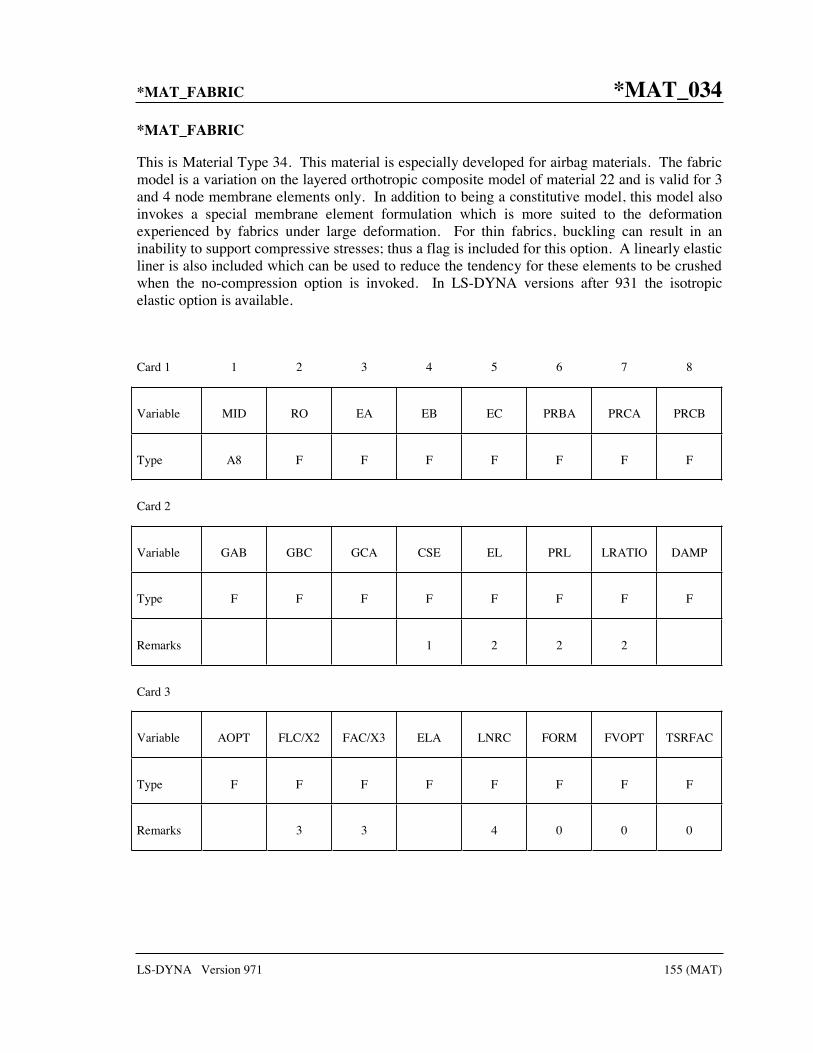
*MAT_FABRIC *MAT_034
LS-DYNA Version 971 155 (MAT)
*MAT_FABRIC
This is Material Type 34. This material is especially developed for airbag materials. The fabric model is a variation on the layered orthotropic composite model of material 22 and is valid for 3 and 4 node membrane elements only. In addition to being a constitutive model, this model also invokes a special membrane element formulation which is more suited to the deformation experienced by fabrics under large deformation. For thin fabrics, buckling can result in an inability to support compressive stresses; thus a flag is included for this option. A linearly elastic liner is also included which can be used to reduce the tendency for these elements to be crushed when the no-compression option is invoked. In LS-DYNA versions after 931 the isotropic elastic option is available.
Card 1 1 2 3 4 5 6 7 8
Variable MID RO EA EB EC PRBA PRCA PRCB
Type A8 F F F F F F F
Card 2
Variable GAB GBC GCA CSE EL PRL LRATIO DAMP
Type F F F F F F F F
Remarks 1 2 2 2
Card 3
Variable AOPT FLC/X2 FAC/X3 ELA LNRC FORM FVOPT TSRFAC
Type F F F F F F F F
Remarks 3 3 4 0 0 0

*MAT_034 *MAT_FABRIC
156 (MAT) LS-DYNA Version 971
Card 4 1 2 3 4 5 6 7 8
Variable A1 A2 A3 X0 X1
Type F F F F F
Card 5
Variable V1 V2 V3 D1 D2 D3 BETA ISREFG
Type F F F F F F F I
Define if and only if FORM=4.
Card 6 1 2 3 4 5 6 7 8
Variable LCA LCB LCAB LCUA LCUB LCUAB
Type I I I I I I
VARIABLE DESCRIPTION
MID Material identification. A unique number or label not exceeding 8 characters must be specified.
RO Mass density.
EA Young’s modulus - longitudinal direction. For an isotopic elastic fabric material only EA and PRBA are defined and are used as the isotropic Young’s modulus and Poisson’s ratio, respectively. The input for the fiber directions and liner should be input as zero for the isotropic elastic fabric.
EB Young’s modulus - transverse direction, set to zero for isotropic elastic material.
(EC) Young’s modulus - normal direction, set to zero for isotropic elastic material. (Not used)

*MAT_FABRIC *MAT_034
LS-DYNA Version 971 157 (MAT)
VARIABLE DESCRIPTION
PRBA νba, Poisson’s ratio ba direction.
(PRCA) νca, Poisson’s ratio ca direction, set to zero for isotropic elastic material. (Not used)
(PRCB) νcb, Poisson’s ratio cb direction, set to zero for isotropic elastic material. (Not used)
GAB Gab, shear modulus ab direction, set to zero for isotropic elastic material.
(GBC) Gbc, shear modulus bc direction, set to zero for isotropic elastic material. (Not used)
(GCA) Gca, shear modulus ca direction, set to zero for isotropic elastic material. (Not used)
CSE Compressive stress elimination option (default 0.0): EQ.0.0: don’t eliminate compressive stresses, EQ.1.0: eliminate compressive stresses (This option does not
apply to the liner).
EL Young’s modulus for elastic liner (optional).
PRL Poisson’s ratio for elastic liner (optional).
LRATIO Ratio of liner thickness to total fabric thickness.
DAMP Rayleigh damping coefficient. A 0.05 coefficient is recommended corresponding to 5% of critical damping. Sometimes larger values are necessary.
AOPT Material axes option (see MAT_OPTION TROPIC_ELASTIC for a more complete description):
EQ.0.0: locally orthotropic with material axes determined by element nodes 1, 2, and 4, as with *DEFINE_COORDINATE_ NODES.
EQ.2.0: globally orthotropic with material axes determined by vectors defined below, as with *DEFINE_COORDINATE_ VECTOR.
EQ.3.0: locally orthotropic material axes determined by rotating the material axes about the element normal by an angle, BETA, from a line in the plane of the element defined by the cross product of the vector v with the element normal.
LT.0.0: the absolute value of AOPT is a coordinate system ID number (CID on *DEFINE_COORDINATE_NODES, *DEFINE_ COORDINATE_SYSTEM or *DEFINE_COORDINATE_ VECTOR). Available in R3 version of 971 and later.
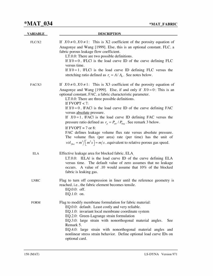
*MAT_034 *MAT_FABRIC
158 (MAT) LS-DYNA Version 971
VARIABLE DESCRIPTION
FLC/X2 If 0 0, 0 1X X≠ ≠ : This is X2 coefficient of the porosity equation of Anagonye and Wang [1999]. Else, this is an optional constant, FLC, a fabric porous leakage flow coefficient.
LT.0.0: There are two possible definitions. If 0 0X = , |FLC| is the load curve ID of the curve defining FLC
versus time. If 0 1X = , |FLC| is the load curve ID defining FLC versus the
stretching ratio defined as 0/sr A A= . See notes below.
FAC/X3 If 0 0, 0 1X X≠ ≠ : This is X3 coefficient of the porosity equation of Anagonye and Wang [1999]. Else, if and only if 0 0X = : This is an optional constant, FAC, a fabric characteristic parameter.
LT.0.0: There are three possible definitions. If FVOPT < 7: If 0 0X = , |FAC| is the load curve ID of the curve defining FAC
versus absolute pressure. If 0 1X = , |FAC| is the load curve ID defining FAC versus the
pressure ratio defined as /p air bagr P P= . See remark 3 below.
If FVOPT = 7 or 8: FAC defines leakage volume flux rate versus absolute pressure.
The volume flux (per area) rate (per time) has the unit of 3 2
fluxvol m m s m s≈ ≈ , equivalent to relative porous gas speed.
ELA Effective leakage area for blocked fabric, ELA. LT.0.0: |ELA| is the load curve ID of the curve defining ELA
versus time. The default value of zero assumes that no leakage occurs. A value of .10 would assume that 10% of the blocked fabric is leaking gas.
LNRC Flag to turn off compression in liner until the reference geometry is reached, i.e., the fabric element becomes tensile.
EQ.0.0: off. EQ.1.0: on.
FORM Flag to modify membrane formulation for fabric material: EQ.0.0: default. Least costly and very reliable. EQ.1.0: invariant local membrane coordinate system EQ.2.0: Green-Lagrange strain formulation EQ.3.0: large strain with nonorthogonal material angles. See
Remark 5. EQ.4.0: large strain with nonorthogonal material angles and
nonlinear stress strain behavior. Define optional load curve IDs on optional card.

*MAT_FABRIC *MAT_034
LS-DYNA Version 971 159 (MAT)
VARIABLE DESCRIPTION
EQ.12.0: Updated form 2. See Remark 10. EQ.13.0: Updated form 3. See Remark 10. EQ.14.0: Updated form 4. See Remark 10.
FVOPT Fabric venting option. EQ.1: Wang-Nefske formulas for venting through an orifice are
used. Blockage is not considered. EQ.2: Wang-Nefske formulas for venting through an orifice are
used. Blockage of venting area due to contact is considered. EQ.3: Leakage formulas of Graefe, Krummheuer, and Siejak [1990]
are used. Blockage is not considered. EQ.4: Leakage formulas of Graefe, Krummheuer, and Siejak [1990]
are used. Blockage of venting area due to contact is considered. EQ.5: Leakage formulas based on flow through a porous media are
used. Blockage is not considered. EQ.6: Leakage formulas based on flow through a porous media are
used. Blockage of venting area due to contact is considered. EQ.7: Leakage is based on gas volume outflow versus pressure load
curve [Lian, 2000]. Blockage is not considered. Absolute pressure is used in the porous-velocity-versus-pressure load curve, given as FAC in the *MAT_FABRIC card.
EQ.8: Leakage is based on gas volume outflow versus pressure load curve [Lian 2000]. Blockage of venting or porous area due to contact is considered. Absolute pressure is used in the porous-velocity-versus-pressure load curve, given as FAC in the *MAT_FABRIC card.
TSRFAC Tensile stress cutoff reduction factor LT.0: |TSRFAC| is the load curve ID of the curve defining
TSRFAC versus time.
A1 A2 A3 Components of vector a for AOPT = 2.
X0,X1 Coefficients of Anagonye and Wang [1999] porosity equation for the
leakage area: ( )0 0 1 2 3leak s p s pA A X X r X r X r r= + + +
V1 V2 V3 Components of vector v for AOPT = 3.
D1 D2 D3 Components of vector d for AOPT = 2.
BETA Material angle in degrees for AOPT = 3, may be overridden on the element card, see *ELEMENT_SHELL_BETA.
ISREFG Initial stress by reference geometry for FORM=12 EQ.0.0: default. Not active.
EQ.1.0: active

*MAT_034 *MAT_FABRIC
160 (MAT) LS-DYNA Version 971
VARIABLE DESCRIPTION
LCA Load curve ID for stress versus strain along the a-axis fiber; available for FORM=4 or 14 only. If zero, EA is used.
LCB Load curve ID for stress versus strain along the b-axis fiber; available for FORM=4 or 14 only. If zero, EB is used.
LCAB Load curve ID for shear stress versus shear strain in the ab-plane; available for FORM=4 or 14 only. If zero, GAB is used.
LCUA Unload/reload curve ID for stress versus strain along the a-axis fiber; available for FORM=4 or 14 only. If zero, LCA is used.
LCUB Unload/reload curve ID for stress versus strain along the b-axis fiber; available for FORM=4 or 14 only. If zero, LCB is used.
LCUAB Unload/reload curve ID for shear stress versus shear strain in the ab-plane; available for FORM=4 or 14 only. If zero, LCAB is used.
Remarks:
1. The no compression option allows the simulation of airbag inflation with far less elements than would be needed for the discretization of the wrinkles which would occur for the case when compressive stresses are not eliminated.
2. When using this material for the analysis of membranes as airbags it is well known from classical theory that only one layer has to be defined. The so-called elastic liner has to be defined for numerical purposes only when the no compression option is invoked.
3. The parameters FLC and FAC are optional for the Wang-Nefske inflation models. It is possible for the airbag to be constructed of multiple fabrics having different values for porosity and permeability. The leakage of gas through the fabric in an airbag then requires an accurate determination of the areas by part ID available for leakage. The leakage area may change over time due to stretching of the airbag fabric or blockage when the bag contacts the structure. LS-DYNA can check the interaction of the bag with the structure and split the areas into regions that are blocked and unblocked depending on whether the regions are in or not in contact, respectively. Typically, FLC and FAC must be determined experimentally and their variations in time or with pressure are optional to allow for maximum flexibility.
4. The elastic backing layer always acts in tension and compression since the tension cutoff option, CSE, does not apply. This can sometimes cause difficulties if the elements are very small in relationship to their actual size as defined by the reference geometry (See *AIRBAG_REFERENCE_GEOMETRY.). If the flag, LNRC, is set to 1.0 the elastic liner does not begin to act until the area of defined by the reference geometry is reached.
5. For FORM=0, 1, and 2, the a-axis and b-axis fiber directions are assumed to be orthogonal and are completely defined by the material axes option, AOPT=0, 2, or 3. For

*MAT_FABRIC *MAT_034
LS-DYNA Version 971 161 (MAT)
FORM=3, 4, 13, or 14, the fiber directions are not assumed orthogonal and must be specified using the ICOMP=1 option on *SECTION_SHELL. Offset angles should be input into the B1 and B2 fields used normally for integration points 1 and 2. The a-axis and b-axis directions will then be offset from the a-axis direction as determined by the material axis option, AOPT=0, 2, or 3.
6. For FORM=4 or 14, nonlinear true stress versus true strain load curves may be defined for a-axis, b-axis, and shear stresses for loading and also for unloading and reloading. All curves should start at the origin and be defined for positive strains only. The a-axis and b-axis stress follows the curves for tension only. For compression, stress is calculated from the constant values, EA or EB. Shear stress/strain behavior is assumed symmetric. If a load curve is omitted, the stress is calculated from the appropriate constant modulus, EA, EB, or GAB.
7. When both loading and unloading curves are defined, the initial yield strain is assumed to be equal to the strain at the first point in the load curve with stress greater than zero. When strain exceeds the yield strain, the stress continues to follow the load curve and the yield strain is updated to the current strain. When unloading occurs, the unload/reload curve is shifted along the x-axis until it intersects the load curve at the current yield strain. If the curve shift is to the right, unloading and reloading will follow the shifted unload/reload curve. If the curve shift is zero or to the left, unloading and reloading will occur along the load curve. When unloading or reloading on the unload curve, the stress is not permitted to fall below the stress calculated by the corresponding constant modulus, EA, EB, or GAB. Therefore, these constant moduli should have slopes that are small relative to the inputted curves to provide a reasonable minimum stress value.
8. The FVOPT flag allows an airbag fabric venting equation to be assigned to an material. The anticipated use for this option is to allow a vent to be defined using FVOPT=1 or 2 for one material and fabric leakage to be defined for using FVOPT=3, 4, 5, or 6 for other materials. In order to use FVOPT, a venting option must first be defined for the airbag using the OPT parameter on *AIRBAG_WANG_NEFSKE or *AIRBAG_HYBRID. If OPT=0, then FVOPT is ignored. If OPT is defined and FVOPT is omitted, then FVOPT is set equal to OPT.
9. The TSRFAC factor is used to assure that airbags that have a reference geometry will open to the correct geometry. Airbags that use a reference geometry might have an initial geometry that results in initial tensile strains. To prevent such strains from prematurely opening an airbag, these tensile strains are eliminated by default. A side effect of this behavior is that airbags that use a reference geometry and that are initially stretched will never achieve the correct shape. The TSRFAC factor is used to restore the tensile strains over time such that the correct geometry is achieved. It is recommend that a load curve be used to define TSRFAC as function of time. Initially the load curve ordinate value should be 0.0 which will allow the bag to remain unstressed. At a time when the bag is partially open, the value of (1.0-TSRFAC) can ramp down to 0.999 which will cause the initially stretched elements to shrink. Permissible values for TSRFAC is 0.0 to 0.001. At this latter value the tensile strains will be removed in 1000 time steps. Larger values than 0.001 may be used but instabilities may occur.

*MAT_034 *MAT_FABRIC
162 (MAT) LS-DYNA Version 971
10. Material forms 12, 13, and 14 are updated versions of forms 2, 3, and 4, respectively. These new forms are intended to be less susceptible to timestep collapse and also guarantee zero stress in the initial geometry when a reference geometry is used. The behavior should otherwise be similar with one exception. The LNRC flag eliminates not only initial compressive strain but total initial strain. Therefore, the TSRFAC option is recommended (see Remark 9) when forms 12, 13, and 14 are used with a reference geometry and LNRC=1.
11 An option to calculate the initial stress by using a reference geometry is available for material FORM 12 only.

*MAT_PLASTIC_GREEN-NAGHDI_RATE *MAT_035
LS-DYNA Version 971 163 (MAT)
*MAT_PLASTIC_GREEN-NAGHDI_RATE
This is Material Type 35. This model is available only for brick elements and is similar to model 3, but uses the Green-Naghdi Rate formulation rather than the Jaumann rate for the stress update. For some cases this might be helpful. This model also has a strain rate dependency following the Cowper-Symonds model.
Card 1 1 2 3 4 5 6 7 8
Variable MID RO E PR
Type A8 F F F
Card 2
Variable SIGY ETAN SRC SRP BETA
Type F F F F F
VARIABLE DESCRIPTION
MID Material identification. A unique number or label not exceeding 8 characters must be specified.
RO Density
E Young’s modulus
PR Poisson’s ratio
SIGY Yield stress
ETAN Plastic hardening modulus
SRC Strain rate parameter, C
SRP Strain rate parameter, P
BETA Hardening parameter, 0 < β′ < 1

*MAT_036 *MAT_3-PARAMETER_BARLAT
164 (MAT) LS-DYNA Version 971
*MAT_3-PARAMETER_BARLAT
This is Material Type 36. This model was developed by Barlat and Lian [1989] for modeling sheets with anisotropic materials under plane stress conditions. This material allows the use of the Lankford parameters for the definition of the anisotropy. This particular development is due to Barlat and Lian [1989]. A version of this material model which has a flow limit diagram failure option is *MAT_FLD_3-PARAMETER_BARLAT.
Card 1 1 2 3 4 5 6 7 8
Variable MID RO E PR HR P1 P2 ITER
Type A8 F F F F F F F
Card 2
Variable M R00 R45 R90 LCID E0 SPI P3
Type F F F F I F F F
Card 3
Variable AOPT C P VLCID
Type F F F I
Card 4
Variable A1 A2 A3
Type F F F

*MAT_3-PARAMETER_BARLAT *MAT_036
LS-DYNA Version 971 165 (MAT)
Card 5 1 2 3 4 5 6 7 8
Variable V1 V2 V3 D1 D2 D3 BETA
Type F F F F F F F
VARIABLE DESCRIPTION
MID Material identification. A unique number or label not exceeding 8 characters must be specified.
RO Mass density.
E Young’s modulus, E GT.0.0: Constant value, LT.0.0: Load curve ID = (-E) which defines Young’s Modulus as
a function of plastic strain. See Remark 1.
PR Poisson’s ratio, ν
HR Hardening rule: EQ.1.0: linear (default), EQ.2.0: exponential (Swift) EQ.3.0: load curve
EQ.4.0: exponential (Voce) EQ.5.0: exponential (Gosh) EQ.6.0: exponential (Hocket-Sherby)
EQ.7.0: load curves in three directions
P1 Material parameter: HR.EQ.1.0: Tangent modulus, HR.EQ.2.0: k, strength coefficient for Swift exponential hardening
HR.EQ.4.0: a, coefficient for Voce exponential hardening HR.EQ.5.0: k, strength coefficient for Gosh exponential hardening HR.EQ.6.0: a, coefficient for Hocket-Sherby exponential hardening
HR.EQ.7.0: load curve ID for hardening in 45 degree direction. See Remark 2.
P2 Material parameter: HR.EQ.1.0: Yield stress HR.EQ.2.0: n, exponent for Swift exponential hardening
HR.EQ.4.0: c, coefficient for Voce exponential hardening HR.EQ.5.0: n, exponent for Gosh exponential hardening HR.EQ.6.0: c. coefficient for Hocket-Sherby exponential hardening
HR.EQ.7.0: load curve ID for hardening in 90 degree direction. See Remark 2.

*MAT_036 *MAT_3-PARAMETER_BARLAT
166 (MAT) LS-DYNA Version 971
VARIABLE DESCRIPTION
ITER Iteration flag for speed: ITER.EQ.0.0: fully iterative ITER.EQ.1.0: fixed at three iterations Generally, ITER=0 is recommended. However, ITER=1 is somewhat
faster and may give acceptable results in most problems.
M m, exponent in Barlat’s yield surface
R00 R00, Lankford parameter in 0 degree direction GT.0.0: Constant value, LT.0.0: Load curve ID = (-R00) which defines R value as a
function of plastic strain. See Remark 3.
R45 R45, Lankford parameter in 45 degree direction GT.0.0: Constant value, LT.0.0: Load curve ID = (-R45) which defines R value as a
function of plastic strain. See Remarks 2 and 3.
R90 R90, Lankford parameter in 90 degree direction GT.0.0: Constant value, LT.0.0: Load curve ID = (-R90) which defines R value as a
function of plastic strain. See Remarks 2 and 3.
LCID Load curve ID for hardening in the 0 degree direction. See Remark 1.
E0 Material parameter HR.EQ.2.0: 0ε for determining initial yield stress for Swift
exponential hardening. (Default=0.0) HR.EQ.4.0: b, coefficient for Voce exponential hardening HR.EQ.5.0: 0ε for determining initial yield stress for Gosh
exponential hardening. (Default=0.0) HR.EQ.6.0: b, coefficient for Hocket-Sherby exponential hardening
SPI spi, if 0ε is zero above and HR.EQ.2.0. (Default=0.0)
EQ.0.0: ( ) ( )0 / ** 1/ 1E k nε = −
LE.0.02: 0 spiε = GT.0.02: ( ) [ ]0 / ** 1/spi k nε = If HR.EQ.5.0 the strain at plastic yield is determined by an iterative
procedure based on the same principles as for HR.EQ.2.0.
P3 Material parameter: HR.EQ.5.0: p, parameter for Gosh exponential hardening HR.EQ.6.0: n, exponent for Hocket-Sherby exponential hardening

*MAT_3-PARAMETER_BARLAT *MAT_036
LS-DYNA Version 971 167 (MAT)
VARIABLE DESCRIPTION
AOPT Material axes option (see MAT_OPTION TROPIC_ELASTIC for a more complete description):
EQ.0.0: locally orthotropic with material axes determined by element nodes 1, 2, and 4, as with *DEFINE_COORDINATE_ NODES.
EQ.2.0: globally orthotropic with material axes determined by vectors defined below, as with *DEFINE_COORDINATE_ VECTOR.
EQ.3.0: locally orthotropic material axes determined by rotating the material axes about the element normal by an angle, BETA, from a line in the plane of the element defined by the cross product of the vector v with the element normal.
LT.0.0: the absolute value of AOPT is a coordinate system ID number (CID on *DEFINE_COORDINATE_NODES, *DEFINE_ COORDINATE_SYSTEM or *DEFINE_COORDINATE_ VECTOR). Available with the R3 release of Version 971 and later.
C C in Cowper-Symonds strain rate model
P p in Cowper-Symonds strain rate model, p=0.0 for no strain rate effects
VLCID Volume correction curve ID defining the relative volume change (change in volume relative to the initial volume) as a function of the effective plastic strain. This is only used when nonzero. See Remark 1.
XP YP ZP Coordinates of point p for AOPT = 1.
A1 A2 A3 Components of vector a for AOPT = 2.
V1 V2 V3 Components of vector v for AOPT = 3.
D1 D2 D3 Components of vector d for AOPT = 2.
BETA Material angle in degrees for AOPT=3, may be overridden on the element card, see *ELEMENT_SHELL_BETA.
Remarks:
1. The effective plastic strain used in this model is defined to be plastic work equivalent. A consequence of this is that for parameters defined as functions of effective plastic strain, the rolling (00) direction should be used as reference direction. For instance, the hardening curve for HR=3 is the stress as function of strain for uniaxial tension in the rolling direction, VLCID curve should give the relative volume change as function of strain for uniaxial tension in the rolling direction and load curve given by -E should give the Young’s modulus as function of strain for uniaxial tension in the rolling direction.

*MAT_036 *MAT_3-PARAMETER_BARLAT
168 (MAT) LS-DYNA Version 971
2. Exceptions from the rule above are curves defined as functions of plastic strain in the 45 and 90 directions, i.e., P1 and P2 for HR=7 and negative R45 or R90. The hardening curves are here defined as measured stress as function of measured plastic strain for uniaxial tension in the direction of interest, i.e., as determined from experimental testing using a standard procedure. Moreover, the curves defining the R values are as function of the measured plastic strain for uniaxial tension in the direction of interest. These curves are transformed internally to be used with the effective stress and strain properties in the actual model. The effective plastic strain does not coincide with the plastic strain components in other directions than the rolling direction and may be somewhat confusing to the user. Therefore the von Mises work equivalent plastic strain is output as history variable #2 if HR=7 or if any of the R-values is defined as function of the plastic strain.
3. The R-values in curves are defined as the ratio of instantaneous width change to instantaneous thickness change. That is, assume that the width W and thickness T are measured as function of strain. Then the corresponding R-value is given by:
/
/
ε
ε
=
dWW
dRdT
Td
4. The anisotropic yield criterion Φ for plane stress is defined as:
1 2 1 2 22 2m m m m
Ya K K a K K c K σΦ = + + − + =
where Yσ is the yield stress and Ki=1,2 are given by:
1
2
2 22
2
2
x y
x yxy
hK
hK p
σ σ
σ στ
+=
−= +
The anisotropic material constants a, c, h, and p are obtained through R00, R45, and R90:
00 90
00 90
2 21 1
R Ra
R R= −
+ +2c a= −
00 90
00 90
1
1
R Rh
R R
+=+
The anisotropy parameter p is calculated implicitly. According to Barlat and Lian the R value, width to thickness strain ratio, for any angle φ can be calculated from:

*MAT_3-PARAMETER_BARLAT *MAT_036
LS-DYNA Version 971 169 (MAT)
21
mY
x y
mRφ
φ
σ
σσ σ
= −∂Φ ∂Φ+∂ ∂
where φσ is the uniaxial tension in the φ direction. This expression can be used to
iteratively calculate the value of p. Let φ =45 and define a function g as
( ) 45
21
mY
x y
mg p R
φ
σ
σσ σ
= − −∂Φ ∂Φ+∂ ∂
An iterative search is used to find the value of p.
For face centered cubic (FCC) materials m=8 is recommended and for body centered cubic (BCC) materials m=6 may be used. The yield strength of the material can be expressed in terms of k and n:
( )nn py ypk kσ ε ε ε= = +
where ypε is the elastic strain to yield and pε is the effective plastic strain (logarithmic). If
SIGY is set to zero, the strain to yield if found by solving for the intersection of the linearly elastic loading equation with the strain hardening equation:
n
E
k
σ εσ ε
=
=
which gives the elastic strain at yield as:
1
1n
yp
E
kε
−=
If SIGY yield is nonzero and greater than 0.02 then:
1
ny
yp k
σε =
The other available hardening models include the Voce equation given by
pcp bea εεσ −−=)(Y ,
the Gosh equation given by
pk npp −+= )()( 0Y εεεσ ,

*MAT_036 *MAT_3-PARAMETER_BARLAT
170 (MAT) LS-DYNA Version 971
and finally the Hocket-Sherby equation given by
npc
p bea εεσ −−=)(Y .
For the Gosh hardening law, the interpretation of the variable SPI is the same, i.e., if set to zero the strain at yield is determined implicitly from the intersection of the strain hardening equation with the linear elastic equation.
To include strain rate effects in the model we multiply the yield stress by a factor depending on the effective plastic strain rate. We use the Cowper-Symonds’ model, hence the yield stress can be written
1/
Y Y( , ) ( ) 1p
psp p p C
εσ ε ε σ ε= +
where sYσ denotes the static yield stress, C and p are material parameters, pε is the
effective plastic strain rate.

*MAT_TRANSVERSELY_ANISOTROPIC_ELASTIC_PLASTIC *MAT_037
LS-DYNA Version 971 171 (MAT)
*MAT_TRANSVERSELY_ANISOTROPIC_ELASTIC_PLASTIC_{OPTION}
Available option allows the change of Young’s Modulus during the simulation:
<BLANK>
ECHANGE
This is Material Type 37. This model is for simulating sheet forming processes with anisotropic material. Only transverse anisotropy can be considered. Optionally an arbitrary dependency of stress and effective plastic strain can be defined via a load curve. This plasticity model is fully iterative and is available only for shell elements. Also see the notes below.
Card 1 1 2 3 4 5 6 7 8
Variable MID RO E PR SIGY ETAN R HLCID
Type A8 F F F F F F F
Define the following card if and only if option ECHANGE is used
Optional 1 2 3 4 5 6 7 8
Variable IDSCALE EA COE
Type I F F
VARIABLE DESCRIPTION
MID Material identification. A unique number or label not exceeding 8 characters must be specified.
RO Mass density.
E Young’s modulus.
PR Poisson’s ratio.
SIGY Yield stress.
ETAN Plastic hardening modulus.
R Anisotropic hardening parameter.

*MAT_037 *MAT_TRANSVERSELY_ANISOTROPIC_ELASTIC_PLASTIC
172 (MAT) LS-DYNA Version 971
VARIABLE DESCRIPTION
HLCID Load curve ID defining effective yield stress versus effective plastic strain.
IDSCALE oad curve ID defining the scale factor for the Young’s modulus change with respect to effective strain (if EA and COE are defined), this curve is not necessary).
EA, COE coefficients defining the Young’s modulus with respect to the effective strain, EA is AE and Coe is ζ (if IDSCALE is defined, these two parameters are not necessary).
Remarks:
Consider Cartesian reference axes which are parallel to the three symmetry planes of anisotropic behavior. Then, the yield function suggested by Hill [1948] can be written
( ) ( ) ( )2 2 2 2 2 222 33 33 11 11 22 23 31 122 2 2 1 0F G H L M Nσ σ σ σ σ σ σ σ σ− + − + − + + + − =
where 1yσ , 2yσ , and 3yσ , are the tensile yield stresses and 12yσ , 23yσ , and 31yσ are the shear
yield stresses. The constants F, G H, L, M, and N are related to the yield stress by
223
231
212
12
12
12
y
y
y
L
M
N
σ
σ
σ
=
=
=
2 2 22 3 1
2 2 23 1 2
2 2 21 2 3
1 1 12
1 1 12
1 1 12 .
y y y
y y y
y y y
F
G
H
σ σ σ
σ σ σ
σ σ σ
= + −
= + −
= + −
The isotropic case of von Mises plasticity can be recovered by setting 2
1
2 y
F G Hσ
= = =
and 2
3
2 y
L M Nσ
= = =

*MAT_TRANSVERSELY_ANISOTROPIC_ELASTIC_PLASTIC *MAT_037
LS-DYNA Version 971 173 (MAT)
For the particular case of transverse anisotropy, where properties do not vary in the x1-x2plane, the following relations hold:
23
2 23
2 23
12 2
2 12
2 1 1
2
y
y y
y y
F G
H
N
σ
σ σ
σ σ
= =
= −
= −
where it has been assumed that 1 2y y yσ σ σ= = .
Letting 3
y
y
Kσσ
= , the yield criteria can be written
( ) e yF σ σ σ= = ,
where
( ) ( ) ( )
( )
2 2 2 2 2 211 22 33 33 11 22 11 22
12
2 2 2 2 223 31 12
2
12 2 2
2y
F K K K
L K
σ σ σ σ σ σ σ σ σ
σ σ σ σ
≡ + + − + − −
+ + + −
The rate of plastic strain is assumed to be normal to the yield surface so pijε is found from
pij
ij
Fε λσ
∂=∂
.
Now consider the case of plane stress, where σ33 = 0. Also, define the anisotropy input parameter, R, as the ratio of the in-plane plastic strain rate to the out-of-plane plastic strain rate,
22
33
p
pR
εε
= .
It then follows that
2
21R
K= − .
Using the plane stress assumption and the definition of R, the yield function may now be written

*MAT_037 *MAT_TRANSVERSELY_ANISOTROPIC_ELASTIC_PLASTIC
174 (MAT) LS-DYNA Version 971
( )1
22 2 211 22 11 22 12
2 2 12
1 1
R RF
R Rσ σ σ σ σ σ+= + − +
+ +.
Note that there are several differences between this model and other plasticity models for shell elements such as the model, MAT_PIECEWISE_LINEAR_PLASTICITY. First, the yield function for plane stress does not include the transverse shear stress components which are updated elastically, and, secondly, this model is always fully iterative. Consequently, in comparing results for the isotropic case where R=1.0 with other isotropic model, differences in the results are expected, even though they are usually insignificant.
The Young’s modulus has been assumed to be constant. Recently, some researchers have found that Young’s modulus decreases with respect to the increase of effective strain. To accommodate this new observation, a new option of _ECHANGE is added. There are two methods defining the change of Young’s modulus change:
The first method is to use a curve to define the scale factor with respect to the effective strain. The value of this scale factor should decrease from 1 to 0 with the increase of effective strain.
The second method is to use a function as proposed by Yoshida [2003]:
0 0 1AE E ( E E )( exp( ))ζ ε= − − − − .

*MAT_BLATZ-KO_FOAM *MAT_038
LS-DYNA Version 971 175 (MAT)
*MAT_BLATZ-KO_FOAM
This is Material Type 38. This model is for the definition of rubber like foams of polyurethane. It is a simple one-parameter model with a fixed Poisson’s ratio of .25.
Card 1 1 2 3 4 5 6 7 8
Variable MID RO G REF
Type A8 F F F
VARIABLE DESCRIPTION
MID Material identification. A unique number or label not exceeding 8 characters must be specified.
RO Mass density.
G Shear modulus.
REF Use reference geometry to initialize the stress tensor. The reference geometry is defined by the keyword:*INITIAL_FOAM_REFERENCE_ GEOMETRY (see there for more details).
EQ.0.0: off, EQ.1.0: on. Remarks:
The strain energy functional for the compressible foam model is given by
II2 III 5
2 III
GW = + −
Blatz and Ko [1962] suggested this form for a 47 percent volume polyurethane foam rubber with a Poisson’s ratio of 0.25. In terms of the strain invariants, I, II, and III, the second Piola-Kirchhoff stresses are given as
( ) 11 IIIII
III IIIij
ij ij ijS G I C Cδ −= − + −
where Cij is the right Cauchy-Green strain tensor. This stress measure is transformed to the Cauchy stress, σij, according to the relationship
-12IIIij
ik jl lkF F Sσ =
where Fij is the deformation gradient tensor.

*MAT_039 *MAT_FLD_TRANSVERSELY_ANISOTROPIC
176 (MAT) LS-DYNA Version 971
*MAT_FLD_TRANSVERSELY_ANISOTROPIC
This is Material Type 39. This model is for simulating sheet forming processes with anisotropic material. Only transverse anisotropy can be considered. Optionally, an arbitrary dependency of stress and effective plastic strain can be defined via a load curve. A Forming Limit Diagram (FLD) can be defined using a curve and is used to compute the maximum strain ratio which can be plotted in LS-Prepost. This plasticity model is fully iterative and is available only for shell elements. Also see the notes below.
Card 1 1 2 3 4 5 6 7 8
Variable MID RO E PR SIGY ETAN R HLCID
Type A8 F F F F F F F
Card 2
Variable LCIDFLD
Type F
VARIABLE DESCRIPTION
MID Material identification. A unique number or label not exceeding 8 characters must be specified.
RO Mass density.
E Young’s modulus.
PR Poisson’s ratio.
SIGY Yield stress.
ETAN Plastic hardening modulus, see notes for model 37.
R Anisotropic hardening parameter, see notes for model 37.
HLCID Load curve ID defining effective stress versus effective plastic strain. The yield stress and hardening modulus are ignored with this option.

*MAT_FLD_TRANSVERSELY_ANISOTROPIC *MAT_039
LS-DYNA Version 971 177 (MAT)
VARIABLE DESCRIPTION
LCIDFLD Load curve ID defining the Forming Limit Diagram. Minor strains in percent are defined as abscissa values and Major strains in percent are defined as ordinate values. The forming limit diagram is shown in Figure 39.1. In defining the curve list pairs of minor and major strains starting with the left most point and ending with the right most point, see *DEFINE_CURVE.
Remarks:
See material model 37 for the theoretical basis. The first history variable is the maximum strain ratio defined by:
workpiece
fld
major
major
εε
corresponding to minorworkpieceε .
Figure 39.1. Forming Limit Diagram.

*MAT_040 *MAT_NONLINEAR_ORTHOTROPIC
178 (MAT) LS-DYNA Version 971
*MAT_NONLINEAR_ORTHOTROPIC
This is Material Type 40. This model allows the definition of an orthotropic nonlinear elastic material based on a finite strain formulation with the initial geometry as the reference. Failure is optional with two failure criteria available. Optionally, stiffness proportional damping can be defined. In the stress initialization phase, temperatures can be varied to impose the initial stresses. This model is only available for shell and solid elements. We do not recommend using this model at this time since it can be unstable especially if the stress-strain curves increase in stiffness with increasing strain.
Card 1 1 2 3 4 5 6 7 8
Variable MID RO EA EB EC PRBA PRCA PRCB
Type A8 F F F F F F F
Default None none none none none none none none
Card 2
Variable GAB GBC GCA DT TRAMP ALPHA
Type F F F F F F
Default None none none 0 0 0
Card 3
Variable LCIDA LCIDB EFAIL DTFAIL CDAMP AOPT MACF
Type F F F F F F I
Default 0.0 0.0 0.0 0.0 0.0 0.0 0

*MAT_NONLINEAR_ORTHOTROPIC *MAT_040
LS-DYNA Version 971 179 (MAT)
Card 4 1 2 3 4 5 6 7 8
Variable XP YP ZP A1 A2 A3
Type F F F F F F
Card 5
Variable V1 V2 V3 D1 D2 D3 BETA
Type F F F F F F F
Optional Card 6 (Applies to Solid elements only)
Card 6 1 2 3 4 5 6 7 8
Variable LCIDC LCIDAB LCIDBC LCIDCA
Type F F F F
Default optional optional optional optional
VARIABLE DESCRIPTION
MID Material identification. A unique number or label not exceeding 8 characters must be specified.
RO Mass density.
EA Ea, Young’s modulus in a-direction.
EB Eb, Young’s modulus in b-direction.
EC Ec, Young’s modulus in c-direction.
PRBA νba, Poisson’s ratio ba.
PRCA νca, Poisson’s ratio ca.
PRCB νcb, Poisson’s ratio cb.

*MAT_040 *MAT_NONLINEAR_ORTHOTROPIC
180 (MAT) LS-DYNA Version 971
VARIABLE DESCRIPTION
GAB Gab, shear modulus ab.
GBC Gbc, shear modulus bc.
GCA Gca, shear modulus ca.
DT Temperature increment for isotropic stress initialization. This option can be used during dynamic relaxation.
TRAMP Time to ramp up to the final temperature.
ALPHA Thermal expansion coefficient.
LCIDA Optional load curve ID defining the nominal stress versus strain along a-axis. Strain is defined as λa-1 where λa is the stretch ratio along the a axis.
LCIDB Optional load curve ID defining the nominal stress versus strain along b-axis. Strain is defined as λb-1 where λb is the stretch ratio along the b axis.
EFAIL Failure strain, λ-1.
DTFAIL Time step for automatic element erosion
CDAMP Damping coefficient.
AOPT Material axes option (see MAT_OPTION TROPIC_ELASTIC for a more complete description):
EQ.0.0: locally orthotropic with material axes determined by element nodes as shown in Figure 2.1. Nodes 1, 2, and 4 of an element are identical to the nodes used for the definition of a coordinate system as by *DEFINE_COORDINATE_NODES.
EQ.1.0: locally orthotropic with material axes determined by a point in space and the global location of the element center; this is the a-direction. This option is for solid elements only.
EQ.2.0: globally orthotropic with material axes determined by vectors defined below, as with *DEFINE_COORDINATE_ VECTOR.
EQ.3.0: locally orthotropic material axes determined by rotating the material axes about the element normal by an angle, BETA, from a line in the plane of the element defined by the cross product of the vector v with the element normal. The plane of a solid element is the midsurface between the inner surface and outer surface defined by the first four nodes and the last four nodes of the connectivity of the element, respectively.

*MAT_NONLINEAR_ORTHOTROPIC *MAT_040
LS-DYNA Version 971 181 (MAT)
VARIABLE DESCRIPTION
EQ.4.0: locally orthotropic in cylindrical coordinate system with the material axes determined by a vector v, and an originating point, P, which define the centerline axis. This option is for solid elements only.
LT.0.0: the absolute value of AOPT is a coordinate system ID number (CID on *DEFINE_COORDINATE_NODES, *DEFINE_ COORDINATE_SYSTEM or *DEFINE_COORDINATE_ VECTOR). Available in R3 version of 971 and later.
MACF Material axes change flag: EQ.1: No change, default, EQ.2: switch material axes a and b, EQ.3: switch material axes a and c, EQ.4: switch material axes b and c.
XP YP ZP Define coordinates of point p for AOPT = 1 and 4.
A1,A2,A3 a1 a2 a3, define components of vector a for AOPT = 2.
D1,D2,D3 d1 d2 d3, define components of vector d for AOPT = 2.
V1,V2,V3 v1 v2 v3, define components of vector v for AOPT = 3 and 4.
BETA Material angle in degrees for AOPT = 3, may be overridden on the element card, see *ELEMENT_SHELL_BETA.
The following input is optional and applies to SOLID ELEMENTS only.
LCIDC Load curve ID defining the nominal stress versus strain along c-axis. Strain is defined as λc-1 where λc is the stretch ratio along the c axis.
LCIDAB Load curve ID defining the nominal ab shear stress versus ab-strain in the ab-plane. Strain is defined as the sin(γab) where γab is the shear angle.
LCIDBC Load curve ID defining the nominal ab shear stress versus ab-strain in the bc-plane. Strain is defined as the sin(γbc) where γbc is the shear angle.
LCIDCA Load curve ID defining the nominal ab shear stress versus ab-strain in the ca-plane. Strain is defined as the sin(γca) where γbc is the shear angle.

*MAT_041-050 *MAT_USER_DEFINED_MATERIAL_MODELS
182 (MAT) LS-DYNA Version 971
*MAT_USER_DEFINED_MATERIAL_MODELS
These are Material Types 41-50. The user can supply his own subroutines. See also Appendix A. The keyword input has to be used for the user interface with data. Isotopic and anisotropic material models with failure can be handled.
Card 1 1 2 3 4 5 6 7 8
Variable MID RO MT LMC NHV IORTHO IBULK IG
Type A8 F I I I I I I
Card 2
Variable IVECT IFAIL ITHERM IHYPER IEOS
Type I I I I I
Define the following two cards if and only if IORTHO=1
Card 3 1 2 3 4 5 6 7 8
Variable AOPT MACF XP YP ZP A1 A2 A3
Type F I F F F F F F
Card 4
Variable V1 V2 V3 D1 D2 D3 BETA
Type F F F F F F F
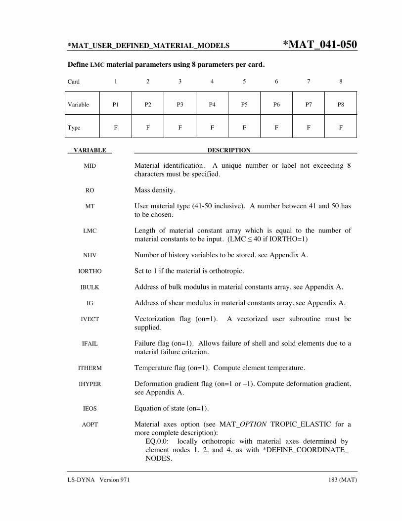
*MAT_USER_DEFINED_MATERIAL_MODELS *MAT_041-050
LS-DYNA Version 971 183 (MAT)
Define LMC material parameters using 8 parameters per card.
Card 1 2 3 4 5 6 7 8
Variable P1 P2 P3 P4 P5 P6 P7 P8
Type F F F F F F F F
VARIABLE DESCRIPTION
MID Material identification. A unique number or label not exceeding 8 characters must be specified.
RO Mass density.
MT User material type (41-50 inclusive). A number between 41 and 50 has to be chosen.
LMC Length of material constant array which is equal to the number of material constants to be input. (LMC 40 if IORTHO=1)
NHV Number of history variables to be stored, see Appendix A.
IORTHO Set to 1 if the material is orthotropic.
IBULK Address of bulk modulus in material constants array, see Appendix A.
IG Address of shear modulus in material constants array, see Appendix A.
IVECT Vectorization flag (on=1). A vectorized user subroutine must be supplied.
IFAIL Failure flag (on=1). Allows failure of shell and solid elements due to a material failure criterion.
ITHERM Temperature flag (on=1). Compute element temperature.
IHYPER Deformation gradient flag (on=1 or –1). Compute deformation gradient, see Appendix A.
IEOS Equation of state (on=1).
AOPT Material axes option (see MAT_OPTION TROPIC_ELASTIC for a more complete description):
EQ.0.0: locally orthotropic with material axes determined by element nodes 1, 2, and 4, as with *DEFINE_COORDINATE_ NODES.

*MAT_041-050 *MAT_USER_DEFINED_MATERIAL_MODELS
184 (MAT) LS-DYNA Version 971
VARIABLE DESCRIPTION
EQ.1.0: locally orthotropic with material axes determined by a point in space and the global location of the element center; this is the a-direction. This option is for solid elements only.
EQ.2.0: globally orthotropic with material axes determined by vectors defined below, as with *DEFINE_COORDINATE_ VECTOR.
EQ.3.0: locally orthotropic material axes determined by rotating the material axes about the element normal by an angle, BETA, from a line in the plane of the element defined by the cross product of the vector v with the element normal.
EQ.4.0: locally orthotropic in cylindrical coordinate system with the material axes determined by a vector v, and an originating point, P, which define the centerline axis. This option is for solid elements only.
LT.0.0: the absolute value of AOPT is a coordinate system ID number (CID on *DEFINE_COORDINATE_NODES, *DEFINE_ COORDINATE_SYSTEM or *DEFINE_COORDINATE_ VECTOR). Available in R3 version of 971 and later.
MACF Material axes change flag for brick elements for quick changes: EQ.1: No change, default, EQ.2: switch material axes a and b, EQ.3: switch material axes a and c, EQ.4: switch material axes b and c.
XP YP ZP Coordinates of point p for AOPT = 1.
A1 A2 A3 Components of vector a for AOPT = 2.
V1 V2 V3 Components of vector v for AOPT = 3.
D1 D2 D3 Components of vector d for AOPT = 2.
BETA Material angle in degrees for AOPT = 3, may be overridden on the element card, see *ELEMENT_SHELL_BETA.
P1 First material parameter.
P2 Second material parameter.
P3 Third material parameter.
P4 Fourth material parameter.
. .
PLMC LMCth material parameter.

*MAT_USER_DEFINED_MATERIAL_MODELS *MAT_041-050
LS-DYNA Version 971 185 (MAT)
Remarks:
1. The material model for the cohesive element (solid element type 19) uses the first two material parameters to set flags for the element formulation. P1 controls how the density is used to calculate the mass. The cohesive element formulation permits the element to have zero or negative volume. Tractions are calculated on a surface midway between the surfaces defined by nodes 1-2-3-4 and 5-6-7-8. If P1 is set to 1.0, then the density is per unit area of the midsurface instead of per unit volume. The second parameter, P2, specifies the number of integration points (one to four) that are required to fail for the element to fail. If it is zero, the element won’t fail regardless of the value of IFAIL. The recommended value of P2 is 1.
2. The cohesive element currently only uses MID, RO, MT, LMC, NHV, IFAIL and IVECT in addition to the material parameters.
3. See Appendix R for the specifics of the umat subroutine requirements for the cohesive element.

*MAT_051 *MAT_BAMMAN
186 (MAT) LS-DYNA Version 971
*MAT_BAMMAN
This is Material Type 51. It allows the modeling of temperature and rate dependent plasticity with a fairly complex model that has many input parameters [Bamman 1989].
Card 1 1 2 3 4 5 6 7 8
Variable MID RO E PR T HC
Type A8 F F F F F
Card 2
Variable C1 C2 C3 C4 C5 C6 C7 C8
Type F F F F F F F F
Card 3
Variable C9 C10 C11 C12 C13 C14 C15 C16
Type F F F F F F F F
Card 4
Variable C17 C18 A1 A2 A4 A5 A6 KAPPA
Type F F F F F F F F
VARIABLE DESCRIPTION
MID Material identification. A unique number or label not exceeding 8 characters must be specified.
RO Mass density.
E Young’s modulus (psi)

*MAT_BAMMAN *MAT_051
LS-DYNA Version 971 187 (MAT)
VARIABLE DESCRIPTION
PR Poisson’s ratio
T Initial temperature (oR)
HC Heat generation coefficient (oR/psi)
C1 Psi
C2 oR
C3 Psi
C4 oR
C5 1/s
C6 oR
C7 1/psi
C8 oR
C9 Psi
C10 oR
C11 1/psi-s
C12 oR
C13 1/psi
C14 oR
C15 psi
C16 oR
C17 1/psi-s
C18 oR
A1 α1, initial value of internal state variable 1
A2 α2, initial value of internal state variable 2. (Note: α3 = -(α1+α2))

*MAT_051 *MAT_BAMMAN
188 (MAT) LS-DYNA Version 971
VARIABLE DESCRIPTION
A3 α4, initial value of internal state variable 3
A4 α5, initial value of internal state variable 4
A5 α6, initial value of internal state variable 5
KAPPA κ, initial value of internal state variable 6
sec-psi-oR sec-MPa-oR sec-MPA-oKC1 *1⁄145 *1⁄145C2 — *5⁄9C3 *1⁄145 *1⁄145
C4 — *5⁄9C5 — — C6 — *5/9C7 *145 *145 C8 — *5⁄9C9 *1⁄145 *1⁄145
C10 — *5⁄9C11 *145 *145 C12 — *5⁄9C13 *145 *145 C14 — *5⁄9C15 *1⁄145 *1⁄145
C16 — *5⁄9C17 *145 *145 C18 — *5⁄9
C0=HC *145 *145*5⁄9E *1⁄145 *1⁄145
υ — — T — *5⁄9

*MAT_BAMMAN *MAT_051
LS-DYNA Version 971 189 (MAT)
Remarks:
The kinematics associated with the model are discussed in references [Hill 1948, Bammann and Aifantis 1987, Bammann 1989]. The description below is taken nearly verbatim from Bammann [1989].
With the assumption of linear elasticity we can write,
( ) tr 1 2o
e eD Dσ λ μ= +
where the Cauchy stress σ is convected with the elastic spin eW as,
oe eW Wσ σ σ σ= − +
This is equivalent to writing the constitutive model with respect to a set of directors whose direction is defined by the plastic deformation [Bammann and Aifantis 1987, Bammann and Johnson 1987]. Decomposing both the skew symmetric and symmetric parts of the velocity gradient into elastic and plastic parts we write for the elastic stretching eD and the elastic spin
eW ,
e p thD D D D= − − , e pW W W= = .
Within this structure it is now necessary to prescribe an equation for the plastic spin pW in addition to the normally prescribed flow rule for pD and the stretching due to the thermal expansion thD . As proposed, we assume a flow rule of the form,
( ) ( )( )sinhp Y T
D f TV T
ξ κ ξξ
− − ′=
′.
where T is the temperature, κ is the scalar hardening variable, and ξ′ is the difference between the deviatoric Cauchy stress σ′ and the tensor variable α′,
ξ σ α′ ′ ′= −
and f(T), Y(T), V(T) are scalar functions whose specific dependence upon the temperature is given below. Assuming isotropic thermal expansion and introducing the expansion coefficient A , the thermal stretching can be written,
1thD AT=
The evolution of the internal variables α and κ are prescribed in a hardening minus recovery format as,

*MAT_051 *MAT_BAMMAN
190 (MAT) LS-DYNA Version 971
( ) ( ) ( )
( ) ( ) ( ) 2
,o
p pd s
p pd s
h T D r T D r T
H T D R T D R T
α α α
κ κ⋅
= − +
= − +
where h and H are the hardening moduli, rs (T) and Rs (T) are scalar functions describing the diffusion controlled ‘static’ or ‘thermal’ recovery, and rd (T) and Rd (T) are the functions describing dynamic recovery.
If we assume that Wp = 0, we recover the Jaumann stress rate which results in the prediction of an oscillatory shear stress response in simple shear when coupled with a Prager kinematic hardening assumption [Johnson and Bammann 1984]. Alternatively we can choose,
1p TW R UU R−= ,
which recovers the Green-Naghdi rate of Cauchy stress and has been shown to be equivalent to Mandel’s isoclinic state [Bammann and Aifantis 1987]. The model employing this rate allows a reasonable prediction of directional softening for some materials, but in general under-predicts the softening and does not accurately predict the axial stresses which occur in the torsion of the thin walled tube.
The final equation necessary to complete our description of high strain rate deformation is one which allows us to compute the temperature change during the deformation. In the absence of a coupled thermo-mechanical finite element code we assume adiabatic temperature change and follow the empirical assumption that 90 -95% of the plastic work is dissipated as heat. Hence,
( ).9 p
v
T DC
σρ
= ⋅ ,
where ρ is the density of the material and Cv the specific heat.
In terms of the input parameters the functions defined above become:
V(T) = C1 exp(-C2/T) h(T) = C9 exp(C10/T) Y(T) = C3 exp(C4/T) rs(T) = C11exp(-C12/T) f(T) = C5 exp(-C6/T) RD(T) = C13exp(-C14/T) rd(T) = C7 exp(-C8/T) H(T) = C15exp(C16/T) RS(T) = C17exp(-C18/T)
and the heat generation coefficient is .9
v
HCCρ
= .
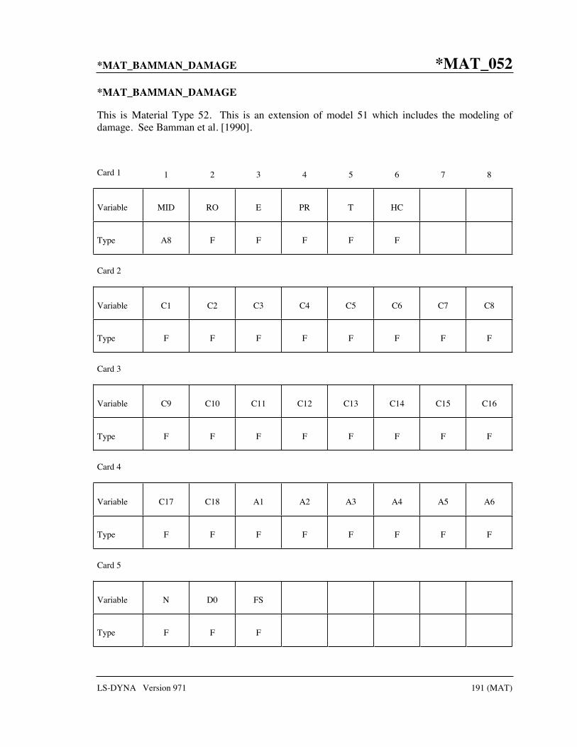
*MAT_BAMMAN_DAMAGE *MAT_052
LS-DYNA Version 971 191 (MAT)
*MAT_BAMMAN_DAMAGE
This is Material Type 52. This is an extension of model 51 which includes the modeling of damage. See Bamman et al. [1990].
Card 1 1 2 3 4 5 6 7 8
Variable MID RO E PR T HC
Type A8 F F F F F
Card 2
Variable C1 C2 C3 C4 C5 C6 C7 C8
Type F F F F F F F F
Card 3
Variable C9 C10 C11 C12 C13 C14 C15 C16
Type F F F F F F F F
Card 4
Variable C17 C18 A1 A2 A3 A4 A5 A6
Type F F F F F F F F
Card 5
Variable N D0 FS
Type F F F

*MAT_052 *MAT_BAMMAN_DAMAGE
192 (MAT) LS-DYNA Version 971
VARIABLE DESCRIPTION
MID Material identification. A unique number or label not exceeding 8 characters must be specified.
RO Mass density
E Young’s modulus (psi)
PR Poisson’s ratio
T Initial temperature (oR)
HC Heat generation coefficient (oR/psi)
C1 Psi
C2 oR
C3 Psi
C4 oR
C5 1/s
C6 oR
C7 1/psi
C8 oR
C9 Psi
C10 oR
C11 1/psi-s
C12 oR
C13 1/psi
C14 oR
C15 psi
C16 oR
C17 1/psi-s
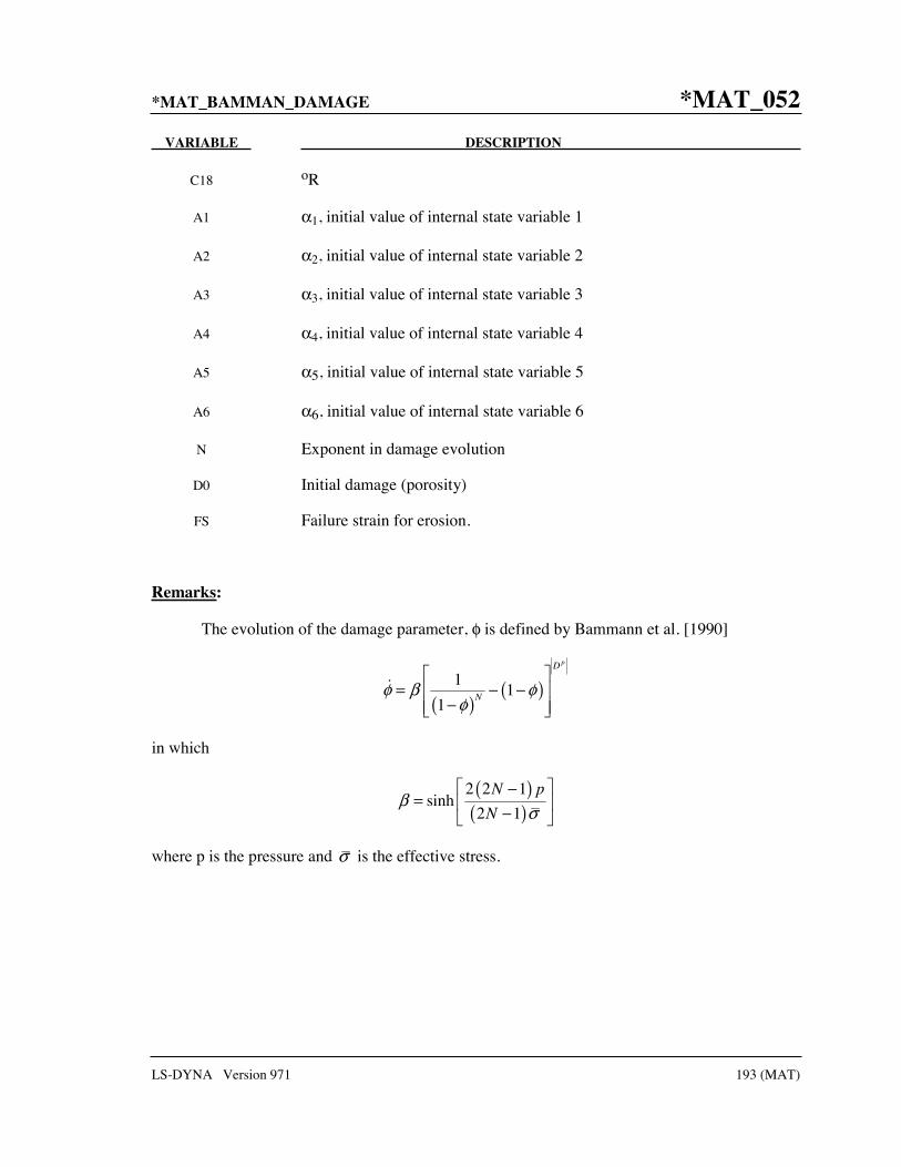
*MAT_BAMMAN_DAMAGE *MAT_052
LS-DYNA Version 971 193 (MAT)
VARIABLE DESCRIPTION
C18 oR
A1 α1, initial value of internal state variable 1
A2 α2, initial value of internal state variable 2
A3 α3, initial value of internal state variable 3
A4 α4, initial value of internal state variable 4
A5 α5, initial value of internal state variable 5
A6 α6, initial value of internal state variable 6
N Exponent in damage evolution
D0 Initial damage (porosity)
FS Failure strain for erosion.
Remarks:
The evolution of the damage parameter, φ is defined by Bammann et al. [1990]
( )( )11
1
pD
Nφ β φφ
= − −−
in which
( )( )
2 2 1sinh
2 1
N p
Nβ
σ−
=−
where p is the pressure and σ is the effective stress.

*MAT_053 *MAT_CLOSED_CELL_FOAM
194 (MAT) LS-DYNA Version 971
*MAT_CLOSED_CELL_FOAM
This is Material Type 53. This allows the modeling of low density, closed cell polyurethane foam. It is for simulating impact limiters in automotive applications. The effect of the confined air pressure is included with the air being treated as an ideal gas. The general behavior is isotropic with uncoupled components of the stress tensor.
Card 1 1 2 3 4 5 6 7 8
Variable MID RO E A B C P0 PHI
Type A8 F F F F F F F
Card 2
Variable GAMA0 LCID
Type F I
VARIABLE DESCRIPTION
MID Material identification. A unique number or label not exceeding 8 characters must be specified.
RO Mass density
E Young’s modulus
A a, factor for yield stress definition, see notes below.
B b, factor for yield stress definition, see notes below.
C c, factor for yield stress definition, see notes below.
P0 Initial foam pressure, P0
PHI Ratio of foam to polymer density, φ
GAMA0 Initial volumetric strain, γ0. The default is zero.

*MAT_CLOSED_CELL_FOAM *MAT_053
LS-DYNA Version 971 195 (MAT)
VARIABLE DESCRIPTION
LCID Optional load curve defining the von Mises yield stress versus γ− . If the load curve ID is given, the yield stress is taken from the curve and the constants a, b, and c are not needed. The load curve is defined in the positive quadrant, i.e., positive values of γ are defined as negative values on the abscissa.
Remarks:
A rigid, low density, closed cell, polyurethane foam model developed at Sandia Laboratories [Neilsen, Morgan and Krieg 1987] has been recently implemented for modeling impact limiters in automotive applications. A number of such foams were tested at Sandia and reasonable fits to the experimental data were obtained.
In some respects this model is similar to the crushable honeycomb model type 26 in that the components of the stress tensor are uncoupled until full volumetric compaction is achieved. However, unlike the honeycomb model this material possesses no directionality but includes the effects of confined air pressure in its overall response characteristics.
sk airij ij ijσ σ δ σ= −
where skijσ is the skeletal stress and airσ is the air pressure computed from the equation:
0
1air p γσ
γ φ= −
+ −
where p0 is the initial foam pressure, usually taken as the atmospheric pressure, and γ defines the volumetric strain
01Vγ γ= − +
where V is the relative volume, defined as the ratio of the current volume to the initial volume, and γ0 is the initial volumetric strain, which is typically zero. The yield condition is applied to the principal skeletal stresses, which are updated independently of the air pressure. We first obtain the skeletal stresses:
sk airij ij ijσ σ σ σ= +
and compute the trial stress, σsktskt skij ij ijE tσ σ ε= + Δ
where E is Young’s modulus. Since Poisson’s ratio is zero, the update of each stress component is uncoupled and 2G=E where G is the shear modulus. The yield condition is applied to the principal skeletal stresses such that, if the magnitude of a principal trial stress component, skt
iσ ,
exceeds the yield stress, σy, then

*MAT_053 *MAT_CLOSED_CELL_FOAM
196 (MAT) LS-DYNA Version 971
( )min ,sktiskti
sk skti y i
σσ
σ σ σ=
The yield stress is defined by
( )1y a b cσ γ= + +
where a, b, and c are user defined input constants and γ is the volumetric strain as defined above. After scaling the principal stresses they are transformed back into the global system and the final stress state is computed
sk airij ij ijσ σ δ σ= − .

*MAT_ENHANCED_COMPOSITE_DAMAGE *MAT_054-055
LS-DYNA Version 971 197 (MAT)
*MAT_ENHANCED_COMPOSITE_DAMAGE
These are Material Types 54-55 which are enhanced versions of the composite model material type 22. Arbitrary orthothropic materials, e.g., unidirectional layers in composite shell structures can be defined. Optionally, various types of failure can be specified following either the suggestions of [Chang and Chang 1987b] or [Tsai and Wu 1971]. In addition special measures are taken for failure under compression. See [Matzenmiller and Schweizerhof 1991]. This model is only valid for thin shell elements. The parameters in parentheses below apply only to solid elements and are therefore always ignored in this material model. They are included for consistency with material types 22 and 59. By using the user defined integration rule, see *INTEGRATION_SHELL, the constitutive constants can vary through the shell thickness. For all shells, except the DKT formulation, laminated shell theory can be activated to properly model the transverse shear deformation. Lamination theory is applied to correct for the assumption of a uniform constant shear strain through the thickness of the shell. For sandwich shells where the outer layers are much stiffer than the inner layers, the response will tend to be too stiff unless lamination theory is used. To turn on lamination theory see *CONTROL_SHELL.
Card 1 1 2 3 4 5 6 7 8
Variable MID RO EA EB (EC) PRBA (PRCA) (PRCB)
Type A8 F F F F F F F
Card 2
Variable GAB GBC GCA (KF) AOPT
Type F F F F F
Card 3
Variable A1 A2 A3 MANGLE
Type F F F F

*MAT_054-055 *MAT_ENHANCED_COMPOSITE_DAMAGE
198 (MAT) LS-DYNA Version 971
Card 4 1 2 3 4 5 6 7 8
Variable V1 V2 V3 D1 D2 D3 DFAILM DFAILS
Type F F F F F F F F
Card 5
Variable TFAIL ALPH SOFT FBRT YCFAC DFAILT DFAILC EFS
Type F F F F F F F F
Card 6
Variable XC XT YC YT SC CRIT BETA
Type F F F F F F F
VARIABLE DESCRIPTION
MID Material identification. A unique number or label not exceeding 8 characters must be specified.
RO Mass density
EA Ea, Young’s modulus - longitudinal direction
EB Eb, Young’s modulus - transverse direction
(EC) Ec, Young’s modulus - normal direction (not used)
PRBA νba, Poisson’s ratio ba
(PRCA) νca, Poisson’s ratio ca (not used)
(PRCB) νcb, Poisson’s ratio cb (not used)
GAB Gab, shear modulus ab
GBC Gbc, shear modulus bc

*MAT_ENHANCED_COMPOSITE_DAMAGE *MAT_054-055
LS-DYNA Version 971 199 (MAT)
VARIABLE DESCRIPTION
GCA Gca, shear modulus ca
(KF) Bulk modulus of failed material (not used)
AOPT Material axes option (see MAT_OPTION TROPIC_ELASTIC for a more complete description):
EQ.0.0: locally orthotropic with material axes determined by element nodes 1, 2, and 4, as with *DEFINE_COORDINATE_ NODES.
EQ.2.0: globally orthotropic with material axes determined by vectors defined below, as with *DEFINE_COORDINATE_ VECTOR.
EQ.3.0: locally orthotropic material axes determined by rotating the material axes about the element normal by an angle (MANGLE) from a line in the plane of the element defined by the cross product of the vector v with the element normal.
LT.0.0: the absolute value of AOPT is a coordinate system ID number (CID on *DEFINE_COORDINATE_NODES, *DEFINE_ COORDINATE_SYSTEM or *DEFINE_COORDINATE_ VECTOR). Available in R3 version of 971 and later.
A1 A2 A3 Define components of vector a for AOPT = 2.
V1 V2 V3 Define components of vector v for AOPT = 3.
D1 D2 D3 Define components of vector d for AOPT = 2.
MANGLE Material angle in degrees for AOPT = 3, may be overridden on the element card, see *ELEMENT_SHELL_BETA or *ELEMENT_ SOLID_ORTHO.
DFAILM Maximum strain for matrix straining in tension or compression (active only for MAT_054 and only if DFAILT > 0). The layer in the element is completely removed after the maximum strain in the matrix direction is reached. The input value is always positive.
DFAILS Maximum shear strain (active only for MAT_054 and only if DFAILT > 0). The layer in the element is completely removed after the maximum shear strain is reached. The input value is always positive.
TFAIL Time step size criteria for element deletion: 0: no element deletion by time step size. The crashfront algorithm
only works if tfail is set to a value above zero. 0 < tfail 0.1: element is deleted when its time step is smaller than
the given value, >.1: element is deleted when the quotient of the actual time step and
the original time step drops below the given value.

*MAT_054-055 *MAT_ENHANCED_COMPOSITE_DAMAGE
200 (MAT) LS-DYNA Version 971
VARIABLE DESCRIPTION
ALPH Shear stress parameter for the nonlinear term, see Material 22.
SOFT Softening reduction factor for material strength in crashfront elements (default = 1.0). TFAIL must be greater than zero to activate this option.
FBRT Softening for fiber tensile strength: EQ.0.0: tensile strength = Xt GT.0.0: tensile strength = Xt, reduced to Xt * FBRT after failure
has occurred in compressive matrix mode.
YCFAC Reduction factor for compressive fiber strength after matrix compressive failure (MAT_054 only). The compressive strength in the fiber direction after compressive matrix failure is reduced to: Xc = YCFAC* Yc (default : YCFAC = 2.0)
DFAILT Maximum strain for fiber tension (MAT_054 only). (Maximum 1 = 100% strain). The layer in the element is completely removed after the maximum tensile strain in the fiber direction is reached. If a nonzero value is given for DFAILT, a nonzero, negative value must also be provided for DFAILC.
DFAILC Maximum strain for fiber compression (MAT_054 only). (Maximum -1 = 100% compression). The layer in the element is completely removed after the maximum compressive strain in the fiber direction is reached. The input value should be negative and is required if DFAILT > 0.
EFS Effective failure strain (MAT_054 only).
XC Longitudinal compressive strength (positive value).
XT Longitudinal tensile strength, see below.
YC Transverse compressive strength, b-axis (positive value), see below.
YT Transverse tensile strength, b-axis, see below.
SC Shear strength, ab plane, see below.
CRIT Failure criterion (material number): EQ.54.0: Chang matrix failure criterion (as Material 22) (default), EQ.55.0: Tsai-Wu criterion for matrix failure.
BETA Weighting factor for shear term in tensile fiber mode (MAT_054 only). (0.0 BETA 1.0)

*MAT_ENHANCED_COMPOSITE_DAMAGE *MAT_054-055
LS-DYNA Version 971 201 (MAT)
Remarks:
The Chang/Chang (mat_54) criteria is given as follows:
for the tensile fiber mode,2
2 00 1
0aa ab
aa ft c
failedthen e
elasticX S
σ σσ β≥
> = + −<
,
Ea = Eb = Gab = νba = νab = 0 ,
for the compressive fiber mode,2
2 00 1
0aa
aa cc
failedthen e
elasticX
σσ≥
< = −<
,
Ea = νba = νab = 0.
for the tensile matrix mode,2 2
2 00 1
0bb ab
bb mt c
failedthen e
elasticY S
σ σσ≥
> = + −<
,
Eb = νba = 0. → Gab = 0 ,
and for the compressive matrix mode,
2 2 2
2 00 1 1
02 2bb c bb ab
bb dc c c c
failedYthen e
elasticS S Y S
σ σ σσ≥
< = + − + −<
,
b = νba = νab = 0. → Gab = 0
Xc = 2Yc for 50% fiber volume.
In the Tsai-Wu (MAT_055) criteria the tensile and compressive fiber modes are treated as in the Chang-Chang criteria. The failure criterion for the tensile and compressive matrix mode is given as:
( )222 0
10
c t bbbb abmd
c t c c t
failedY Ye
elasticY Y S Y Y
σσ σ ≥−= + + −
<
For β=1 we get the original criterion of Hashin [1980] in the tensile fiber mode. For β=0 we get the maximum stress criterion which is found to compare better to experiments.
In MAT_054, failure can occur in any of four different ways:
1. If DFAILT is zero, failure occurs if the Chang-Chang failure criterion is satisfied in the tensile fiber mode.

*MAT_054-055 *MAT_ENHANCED_COMPOSITE_DAMAGE
202 (MAT) LS-DYNA Version 971
2. If DFAILT is greater than zero, failure occurs if the tensile fiber strain is greater than DFAILT or less than DFAILC.
3. If EFS is greater than zero, failure occurs if the effective strain is greater than EFS.
4. If TFAIL is greater than zero, failure occurs according to the element timestep as described in the definition of TFAIL above.
When failure has occurred in all the composite layers (through-thickness integration points), the element is deleted. Elements which share nodes with the deleted element become “crashfront” elements and can have their strengths reduced by using the SOFT parameter with TFAIL greater than zero.
Information about the status in each layer (integration point) and element can be plotted using additional integration point variables. The number of additional integration point variables for shells written to the LS-DYNA database is input by the *DATABASE_EXTENT_BINARY definition as variable NEIPS. For Models 54 and 55 these additional variables are tabulated below (i = shell integration point):
History
Variable
Description Value LS-Prepost
history variable
1.ef i( ) tensile fiber mode 1 2.ec i( ) compressive fiber mode 1 - elastic 2 3.em i( ) tensile matrix mode 0 - failed 3 4.ed i( ) compressive matrix mode 4 5.efail max[ef(ip)] 5
6.dam damage parameter
-1 - element intact 10-8 - element in crashfront
+1 – element failed 6
These variables can be plotted in LS-Prepost element history variables 1 to 6. The following components, defined by the sum of failure indicators over all through-thickness integration points, are stored as element component 7 instead of the effective plastic strain.
Description Integration point
( )1
1 nip
i
ef inip =
1
( )1
1 nip
i
ec inip =
2
( )1
1 nip
i
em inip =
3

*MAT_LOW_DENSITY_FOAM *MAT_057
LS-DYNA Version 971 203 (MAT)
*MAT_LOW_DENSITY_FOAM
This is Material Type 57 for modeling highly compressible low density foams. Its main applications are for seat cushions and padding on the Side Impact Dummies (SID). Optionally, a tension cut-off failure can be defined. Also, see the notes below.
Card 1 1 2 3 4 5 6 7 8
Variable MID RO E LCID TC HU BETA DAMP
Type A8 F F F F F F F
Default --- --- --- --- 1.E+20 1. 0.05
Remarks --- --- --- --- --- 3 1 ---
Card 2
Variable SHAPE FAIL BVFLAG ED BETA1 KCON REF
Type F F F F F F F
Default 1.0 0.0 0.0 0.0 0.0 0.0 0.0
Remarks 3 --- 2 5 5 6
VARIABLE DESCRIPTION
MID Material identification. A unique number or label not exceeding 8 characters must be specified.
RO Mass density
E Young’s modulus used in tension. For implicit problems E is set to the initial slope of load curve LCID.
LCID Load curve ID, see *DEFINE_CURVE, for nominal stress versus strain.
TC Tension cut-off stress

*MAT_057 *MAT_LOW_DENSITY_FOAM
204 (MAT) LS-DYNA Version 971
VARIABLE DESCRIPTION
HU Hysteretic unloading factor between 0 and 1 (default=1, i.e., no energy dissipation), see also Figure 57.1.
BETA β, decay constant to model creep in unloading
DAMP Viscous coefficient (.05< recommended value <.50) to model damping effects.
LT.0.0: |DAMP| is the load curve ID, which defines the damping constant as a function of the maximum strain in compression defined as:
εmax = max(1 − λ1,1 − λ2,1. − λ3 ) .
In tension, the damping constant is set to the value corresponding to the strain at 0. The abscissa should be defined from 0 to 1.
SHAPE Shape factor for unloading. Active for nonzero values of the hysteretic unloading factor. Values less than one reduces the energy dissipation and greater than one increases dissipation, see also Figure 57.1.
FAIL Failure option after cutoff stress is reached: EQ.0.0: tensile stress remains at cut-off value, EQ.1.0: tensile stress is reset to zero.
BVFLAG Bulk viscosity activation flag, see remark below: EQ.0.0: no bulk viscosity (recommended), EQ.1.0: bulk viscosity active.
ED Optional Young's relaxation modulus, Ed , for rate effects. See comments below.
BETA1 Optional decay constant, β1.
KCON Stiffness coefficient for contact interface stiffness. If undefined the maximum slope in stress vs. strain curve is used. When the maximum slope is taken for the contact, the time step size for this material is reduced for stability. In some cases Δt may be significantly smaller, and defining a reasonable stiffness is recommended.
REF Use reference geometry to initialize the stress tensor. The reference geometry is defined by the keyword:*INITIAL_FOAM_REFERENCE_ GEOMETRY (see there for more details).
EQ.0.0: off, EQ.1.0: on.

*MAT_LOW_DENSITY_FOAM *MAT_057
LS-DYNA Version 971 205 (MAT)
Remarks:
The compressive behavior is illustrated in Figure 57.1 where hysteresis on unloading is shown. This behavior under uniaxial loading is assumed not to significantly couple in the transverse directions. In tension the material behaves in a linear fashion until tearing occurs. Although our implementation may be somewhat unusual, it was motivated by Storakers [1986].
The model uses tabulated input data for the loading curve where the nominal stresses are defined as a function of the elongations, εi, which are defined in terms of the principal stretches, λi, as:
εi = λi – 1
The stretch ratios are found by solving for the eigenvalues of the left stretch tensor, Vij, which is obtained via a polar decomposition of the deformation gradient matrix, Fij. Recall that,
Fij = RikUkj = VikRkj
The update of Vij follows the numerically stable approach of Taylor and Flanagan [1989]. After solving for the principal stretches, we compute the elongations and, if the elongations are compressive, the corresponding values of the nominal stresses, τi are interpolated. If the elongations are tensile, the nominal stresses are given by
τi = Eεi
and the Cauchy stresses in the principal system become
ii
j k
τσλ λ
=
The stresses can now be transformed back into the global system for the nodal force calculations.
Additional Remarks:
1. When hysteretic unloading is used the reloading will follow the unloading curve if the decay constant, β, is set to zero. If β is nonzero the decay to the original loading curve is governed by the expression:
1. - e-βt
2. The bulk viscosity, which generates a rate dependent pressure, may cause an unexpected volumetric response and, consequently, it is optional with this model.
3. The hysteretic unloading factor results in the unloading curve to lie beneath the loading curve as shown in Figure 57.1. This unloading provides energy dissipation which is reasonable in certain kinds of foam.
4. Note that since this material has no effective plastic strain, the internal energy per initial volume is written into the output databases.

*MAT_057 *MAT_LOW_DENSITY_FOAM
206 (MAT) LS-DYNA Version 971
5. Rate effects are accounted for through linear viscoelasticity by a convolution integral of the form
( )0
tr klij ijklg t d
∂εσ τ τ∂τ
= −
where gijkl(t − τ ) is the relaxation function. The stress tensor, σ ijr , augments the stresses
determined from the foam, σ ijf ; consequently, the final stress, σ ij , is taken as the
summation of the two contributions:
σ ij = σ ijf + σ ij
r .
Since we wish to include only simple rate effects, the relaxation function is represented by one term from the Prony series:
g( t) = α0 + α mm =1
N
e−β t
given by,
g( t) = Ede−β1 t
This model is effectively a Maxwell fluid which consists of a damper and spring in series. We characterize this in the input by a Young's modulus, Ed , and decay constant, β1 . The formulation is performed in the local system of principal stretches where only the principal values of stress are computed and triaxial coupling is avoided. Consequently, the one-dimensional nature of this foam material is unaffected by this addition of rate effects. The addition of rate effects necessitates twelve additional history variables per integration point. The cost and memory overhead of this model comes primarily from the need to “remember” the local system of principal stretches.
Figure 57.1. Behavior of the low density urethane foam model.
6. The time step size is based on the current density and the maximum of the instantaneous loading slope, E, and KCON. If KCON is undefined the maximum slope in the loading curve is used instead.
Typical unloading curves determined by the hysteretic unloading factor with a shape factor equal to unity.
Typical unloading for a large shape factor, e.g., 5.0 – 8.0, and a small hysteretic unloading factor, e.g., 0.01.

*MAT_LAMINATED_COMPOSITE_FABRIC *MAT_058
LS-DYNA Version 971 207 (MAT)
*MAT_LAMINATED_COMPOSITE_FABRIC
This is Material Type 58. Depending on the type of failure surface, this model may be used to model composite materials with unidirectional layers, complete laminates, and woven fabrics. This model is implemented for shell and thick shell elements.
Card 1 1 2 3 4 5 6 7 8
Variable MID RO EA EB (EC) PRBA TAU1 GAMMA1
Type A8 F F F F F F F
Card 2
Variable GAB GBC GCA SLIMT1 SLIMC1 SLIMT2 SLIMC2 SLIMS
Type F F F F F F F F
Card 3
Variable AOPT TSIZE ERODS SOFT FS
Type F F F F F
Card 4
Variable XP YP ZP A1 A2 A3
Type F F F F F F

*MAT_058 *MAT_LAMINATED_COMPOSITE_FABRIC
208 (MAT) LS-DYNA Version 971
Card 5 1 2 3 4 5 6 7 8
Variable V1 V2 V3 D1 D2 D3 BETA
Type F F F F F F F
Card 6
Variable E11C E11T E22C E22T GMS
Type F F F F F
Card 7
Variable XC XT YC YT SC
Type F F F F F
VARIABLE DESCRIPTION
MID Material identification. A unique number or label not exceeding 8 characters must be specified.
RO Mass density
EA Ea, Young’s modulus - longitudinal direction
EB Eb, Young’s modulus - transverse direction
(EC) Ec, Young’s modulus - normal direction (not used)
PRBA νba, Poisson’s ratio ba
TAU1 τ1, stress limit of the first slightly nonlinear part of the shear stress versus shear strain curve. The values τ1 and γ1 are used to define a curve of shear stress versus shear strain. These values are input if FS, defined below, is set to a value of -1.
GAMMA1 γ1, strain limit of the first slightly nonlinear part of the shear stress versus shear strain curve.

*MAT_LAMINATED_COMPOSITE_FABRIC *MAT_058
LS-DYNA Version 971 209 (MAT)
VARIABLE DESCRIPTION
GAB Gab, shear modulus ab
GBC Gbc, shear modulus bc
GCA Gca, shear modulus ca
SLIMT1 Factor to determine the minimum stress limit after stress maximum (fiber tension).
SLIMC1 Factor to determine the minimum stress limit after stress maximum (fiber compression).
SLIMT2 Factor to determine the minimum stress limit after stress maximum (matrix tension).
SLIMC2 Factor to determine the minimum stress limit after stress maximum (matrix compression).
SLIMS Factor to determine the minimum stress limit after stress maximum (shear).
AOPT Material axes option (see MAT_OPTION TROPIC_ELASTIC for a more complete description):
EQ. 0.0: locally orthotropic with material axes determined by element nodes 1, 2, and 4, as with *DEFINE_COORDINATE_ NODES.
EQ. 2.0: globally orthotropic with material axes determined by vectors defined below, as with *DEFINE_COORDINATE_ VECTOR.
EQ. 3.0: locally orthotropic material axes determined by rotating the material axes about the element normal by an angle (BETA) from a line in the plane of the element defined by the cross product of the vector v with the element normal.
LT.0.0: the absolute value of AOPT is a coordinate system ID number (CID on *DEFINE_COORDINATE_NODES, *DEFINE_ COORDINATE_SYSTEM or *DEFINE_COORDINATE_ VECTOR). Available in R3 version of 971 and later.
TSIZE Time step for automatic element deletion.
ERODS Maximum effective strain for element layer failure. A value of unity would equal 100% strain.
SOFT Softening reduction factor for strength in the crashfront.

*MAT_058 *MAT_LAMINATED_COMPOSITE_FABRIC
210 (MAT) LS-DYNA Version 971
VARIABLE DESCRIPTION
FS Failure surface type: EQ.1.0: smooth failure surface with a quadratic criterion for both
the fiber (a) and transverse (b) directions. This option can be used with complete laminates and fabrics.
EQ.0.0: smooth failure surface in the transverse (b) direction with a limiting value in the fiber (a) direction. This model is appropriate for unidirectional (UD) layered composites only.
EQ.-1.: faceted failure surface. When the strength values are reached then damage evolves in tension and compression for both the fiber and transverse direction. Shear behavior is also considered. This option can be used with complete laminates and fabrics.
XP YP ZP Define coordinates of point p for AOPT = 1.
A1 A2 A3 Define components of vector a for AOPT = 2.
V1 V2 V3 Define components of vector v for AOPT = 3.
D1 D2 D3 Define components of vector d for AOPT = 2.
BETA Material angle in degrees for AOPT=3, may be overridden on the element card, see *ELEMENT_SHELL_BETA.
E11C Strain at longitudinal compressive strength, a-axis (positive).
E11T Strain at longitudinal tensile strength, a-axis.
E22C Strain at transverse compressive strength, b-axis.
E22T Strain at transverse tensile strength, b-axis.
GMS Strain at shear strength, ab plane.
XC Longitudinal compressive strength (positive value).
XT Longitudinal tensile strength, see below.
YC Transverse compressive strength, b-axis (positive value), see below.
YT Transverse tensile strength, b-axis, see below.
SC Shear strength, ab plane, see below.

*MAT_LAMINATED_COMPOSITE_FABRIC *MAT_058
LS-DYNA Version 971 211 (MAT)
Remarks:
Parameters to control failure of an element layer are: ERODS, the maximum effective strain, i.e., maximum 1 = 100 % straining. The layer in the element is completely removed after the maximum effective strain (compression/tension including shear) is reached.
The stress limits are factors used to limit the stress in the softening part to a given value,
σmin = SLIMxx ⋅strength ,
thus, the damage value is slightly modified such that elastoplastic like behavior is achieved with the threshold stress. As a factor for SLIMxx a number between 0.0 and 1.0 is possible. With a factor of 1.0, the stress remains at a maximum value identical to the strength, which is similar to ideal elastoplastic behavior. For tensile failure a small value for SLIMTx is often reasonable; however, for compression SLIMCx = 1.0 is preferred. This is also valid for the corresponding shear value. If SLIMxx is smaller than 1.0 then localization can be observed depending on the total behavior of the lay-up. If the user is intentionally using SLIMxx < 1.0, it is generally recommended to avoid a drop to zero and set the value to something in between 0.05 and 0.10. Then elastoplastic behavior is achieved in the limit which often leads to less numerical problems. Defaults for SLIMXX = 1.0E-8.
The crashfront-algorithm is started if and only if a value for TSIZE (time step size, with element elimination after the actual time step becomes smaller than TSIZE) is input.
The damage parameters can be written to the postprocessing database for each integration point as the first three additional element variables and can be visualized.
Material models with FS=1 or FS=-1 are favorable for complete laminates and fabrics, as all directions are treated in a similar fashion.
For material model FS=1 an interaction between normal stresses and the shear stresses is assumed for the evolution of damage in the a and b-directions. For the shear damage is always the maximum value of the damage from the criterion in a or b-direction is taken.
For material model FS=-1 it is assumed that the damage evolution is independent of any of the other stresses. A coupling is only present via the elastic material parameters and the complete structure.
In tensile and compression directions and in a as well as in b- direction different failure surfaces can be assumed. The damage values, however, increase only also when the loading direction changes.
Special control of shear behavior of fabrics
For fabric materials a nonlinear stress strain curve for the shear part for failure surface FS=-1 can be assumed as given below. This is not possible for other values of FS.
The curve, shown in Figure 58.1 is defined by three points:

*MAT_058 *MAT_LAMINATED_COMPOSITE_FABRIC
212 (MAT) LS-DYNA Version 971
a) the origin (0,0) is assumed,
b) the limit of the first slightly nonlinear part (must be input), stress (TAU1) and strain (GAMMA1), see below.
c) the shear strength at failure and shear strain at failure.
In addition a stress limiter can be used to keep the stress constant via the SLIMS parameter. This value must be less or equal 1.0 but positive, and leads to an elastoplastic behavior for the shear part. The default is 1.0E-08, assuming almost brittle failure once the strength limit SC is reached.
Figure 58.1. Stress-strain diagram for shear.

*MAT_COMPOSITE_FAILURE_OPTION_MODEL *MAT_059
LS-DYNA Version 971 213 (MAT)
*MAT_COMPOSITE_FAILURE_OPTION_MODEL
This is Material Type 59.
Available options include:
SHELL
SOLID
depending on the element type the material is to be used with, see *PART.
For both options define cards 1 to 4 below
Card 1 1 2 3 4 5 6 7 8
Variable MID RO EA EB EC PRBA PRCA PRCB
Type A8 F F F F F F F
Card 2
Variable GAB GBC GCA KF AOPT MACF
Type F F F F F I
Card 3
Variable XP YP ZP A1 A2 A3
Type F F F F F F
Card 4
Variable V1 V2 V3 D1 D2 D3 BETA
Type F F F F F F F

*MAT_059 *MAT_COMPOSITE_FAILURE_OPTION_MODEL
214 (MAT) LS-DYNA Version 971
Cards 5 and 6 for SHELL option
Card 5 1 2 3 4 5 6 7 8
Variable TSIZE ALP SOFT FBRT SR SF
Type F F F F F F
Card 6
Variable XC XT YC YT SC
Type F F F F F
Cards 5 and 6 for SOLID option
Card 5 1 2 3 4 5 6 7 8
Variable SBA SCA SCB XXC YYC ZZC
Type F F F F F F
Card 6
Variable XXT YYT ZZT
Type F F F

*MAT_COMPOSITE_FAILURE_OPTION_MODEL *MAT_059
LS-DYNA Version 971 215 (MAT)
VARIABLE DESCRIPTION
MID Material identification. A unique number or label not exceeding 8 characters must be specified.
RO Density
EA Ea, Young’s modulus - longitudinal direction
EB Eb, Young’s modulus - transverse direction
EC Ec, Young’s modulus - normal direction
PRBA νba Poisson’s ratio ba
PRCA νca Poisson’s ratio ca
PRCB νcb Poisson’s ratio cb
GAB Gab Shear Modulus
GBC Gbc Shear Modulus
GCA Gca Shear Modulus
KF Bulk modulus of failed material
AOPT Material axes option (see MAT_OPTION TROPIC_ELASTIC for a more complete description):
EQ.0.0: locally orthotropic with material axes determined by element nodes 1, 2, and 4, as with *DEFINE_COORDINATE_ NODES.
EQ.1.0: locally orthotropic with material axes determined by a point in space and the global location of the element center; this is the a-direction. This option is for solid elements only.
EQ.2.0: globally orthotropic with material axes determined by vectors defined below, as with *DEFINE_COORDINATE_ VECTOR.
EQ.3.0: locally orthotropic material axes determined by rotating the material axes about the element normal by an angle, BETA, from a line in the plane of the element defined by the cross product of the vector v with the element normal.
EQ.4.0: locally orthotropic in cylindrical coordinate system with the material axes determined by a vector v, and an originating point, P, which define the centerline axis. This option is for solid elements only.

*MAT_059 *MAT_COMPOSITE_FAILURE_OPTION_MODEL
216 (MAT) LS-DYNA Version 971
VARIABLE DESCRIPTION
LT.0.0: the absolute value of AOPT is a coordinate system ID number (CID on *DEFINE_COORDINATE_NODES, *DEFINE_ COORDINATE_SYSTEM or *DEFINE_COORDINATE_ VECTOR). Available in R3 version of 971 and later.
XP YP ZP Define coordinates of point p for AOPT = 1 and 4.
A1 A2 A3 Define components of vector a for AOPT = 2.
V1 V2 V3 Define components of vector v for AOPT = 3 and 4.
D1 D2 D3 Define components of vector d for AOPT = 2:
BETA Material angle in degrees for AOPT=3, may be overridden on the element card, see *ELEMENT_SHELL_BETA or *ELEMENT_ SOLID_ORTHO.
MACF Material axes change flag for brick elements. EQ.1: No change, default, EQ.2: switch material axes a and b, EQ.3: switch material axes a and c, EQ.4: switch material axes b and c.
BETA Material angle in degrees for AOPT = 3, may be overridden on the element card, see *ELEMENT_SHELL_BETA.
TSIZE Time step for automatic element deletion
ALP Nonlinear shear stress parameter
SOFT Softening reduction factor for strength in crush
FBRT Softening of fiber tensile strength
SR sr, reduction factor (default=0.447)
SF sf, softening factor (default=0.0)
XC Longitudinal compressive strength, a-axis (positive value).
XT Longitudinal tensile strength, a-axis
YC Transverse compressive strength, b-axis (positive value).
YT Transverse tensile strength, b-axis

*MAT_COMPOSITE_FAILURE_OPTION_MODEL *MAT_059
LS-DYNA Version 971 217 (MAT)
VARIABLE DESCRIPTION
SC Shear strength, ab plane: GT.0.0 faceted failure surface theory, LT.0.0 ellipsoidal failure surface theory.
SBA In plane shear strength.
SCA Transverse shear strength.
SCB Transverse shear strength.
XXC Longitudinal compressive strength a-axis (positive value).
YYC Transverse compressive strength b-axis (positive value).
ZZC Normal compressive strength c-axis (positive value).
XXT Longitudinal tensile strength a-axis.
YYT Transverse tensile strength b-axis.
ZZT Normal tensile strength c-axis.

*MAT_060 *MAT_ELASTIC_WITH_VISCOSITY
218 (MAT) LS-DYNA Version 971
*MAT_ELASTIC_WITH_VISCOSITY
This is Material Type 60 which was developed to simulate forming of glass products (e.g., car windshields) at high temperatures. Deformation is by viscous flow but elastic deformations can also be large. The material model, in which the viscosity may vary with temperature, is suitable for treating a wide range of viscous flow problems and is implemented for brick and shell elements.
Card 1 1 2 3 4 5 6 7 8
Variable MID RO V0 A B C LCID
Type A8 F F F F F F
Card 2
Variable PR1 PR2 PR3 PR4 PR5 PR6 PR7 PR8
Type F F F F F F F F
Card 3
Variable T1 T2 T3 T4 T5 T6 T7 T8
Type F F F F F F F F
Card 4
Variable V1 V2 V3 V4 V5 V6 V7 V8
Type F F F F F F F F

*MAT_ELASTIC_WITH_VISCOSITY *MAT_060
LS-DYNA Version 971 219 (MAT)
Card 5 1 2 3 4 5 6 7 8
Variable E1 E2 E3 E4 E5 E6 E7 E8
Type F F F F F F F F
Card 6
Variable ALPHA1 ALPHA2 ALPHA3 ALPHA4 ALPHA5 ALPHA6 ALPHA7 ALPHA8
Type F F F F F F F F
VARIABLE DESCRIPTION
MID Material identification. A unique number or label not exceeding 8 characters must be specified.
RO Mass density
V0 Temperature independent viscosity coefficient, V0. If defined, the temperature dependent viscosity defined below is skipped, see type (i) and (ii) definitions for viscosity below.
A Viscosity coefficient, see type (i) and (ii) definitions for viscosity below.
B Viscosity coefficient, see type (i) and (ii) definitions for viscosity below.
C Viscosity coefficient, see type (i) and (ii) definitions for viscosity below.
LCID Load curve (see *DEFINE_CURVE) defining viscosity versus temperature, see type (iii). (Optional)
T1, T2,...TN Temperatures, define up to 8 values
PR1, PR2,...PRN Poisson’s ratios for the temperatures Ti
V1, V2,...VN Corresponding viscosity coefficients (define only one if not varying with temperature)
E1, E2,...EN Corresponding Young’s moduli coefficients (define only one if not varying with temperature)
ALPHA.... Corresponding thermal expansion coefficients

*MAT_060 *MAT_ELASTIC_WITH_VISCOSITY
220 (MAT) LS-DYNA Version 971
Remarks:
Volumetric behavior is treated as linear elastic. The deviatoric strain rate is considered to be the sum of elastic and viscous strain rates:
~ ~ ~ 2 2total elastic viscous G v
σ σε ε ε ′ ′′ ′ ′= + = +
where G is the elastic shear modulus, v is the viscosity coefficient, and ~ indicates a tensor. The stress increment over one timestep dt is
2 total
Gd G dt dtσ ε σ
υ′ ′ ′= −
The stress before the update is used for σ ′ . For shell elements the through-thickness strain rate is calculated as follows.
11 22 33 3333 330 2G
d K dt G dt dtσ ε ε ε ε συ
′ ′= = + + + −
where the subscript ij = 33 denotes the through-thickness direction and K is the elastic bulk modulus. This leads to:
33 11 22a bpε ε ε= − + +
2343
K Ga
K G
−=
+
( )43
Gdtb
K Gυ=
+
in which p is the pressure defined as the negative of the hydrostatic stress.
The variation of viscosity with temperature can be defined in any one of the 3 ways.
(i) Constant, V = V0 Do not define constants, A, B, and C or the piecewise curve.(leave card 4 blank)
(ii) V = V0 × 10** (A/(T-B) + C)
(iii) Piecewise curve: define the variation of viscosity with temperature.
Note: Viscosity is inactive during dynamic relaxation.

*MAT_ELASTIC_WITH_VISCOSITY_CURVE *MAT_060C
LS-DYNA Version 971 221 (MAT)
*MAT_ELASTIC_WITH_VISCOSITY_CURVE
This is Material Type 60 which was developed to simulate forming of glass products (e.g., car windshields) at high temperatures. Deformation is by viscous flow but elastic deformations can also be large. The material model, in which the viscosity may vary with temperature, is suitable for treating a wide range of viscous flow problems and is implemented for brick and shell elements. Load curves are used to represent the temperature dependence of Poisson’s ratio, Young’s modulus, the coefficient of expansion, and the viscosity.
Card 1 1 2 3 4 5 6 7 8
Variable MID RO V0 A B C LCID
Type A8 F F F F F F
Card 2
Variable PR_LC YM_LC A_LC V_LC V_LOG
Type F F F F F
VARIABLE DESCRIPTION
MID Material identification. A unique number or label not exceeding 8 characters must be specified.
RO Mass density
V0 Temperature independent viscosity coefficient, V0. If defined, the temperature dependent viscosity defined below is skipped, see type (i) and (ii) definitions for viscosity below.
A Viscosity coefficient, see type (i) and (ii) definitions for viscosity below.
B Viscosity coefficient, see type (i) and (ii) definitions for viscosity below.
C Viscosity coefficient, see type (i) and (ii) definitions for viscosity below.
LCID Load curve (see *DEFINE_CURVE) defining factor on viscosity versus temperature, see type (iii). (Optional).
PR_LC Load curve (see *DEFINE_CURVE) defining Poisson’s ratio as a function of temperature.

*MAT_060C *MAT_ELASTIC_WITH_VISCOSITY_CURVE
222 (MAT) LS-DYNA Version 971
VARIABLE DESCRIPTION
YM_LC Load curve (see *DEFINE_CURVE) defining Young’s modulus as a function of temperature.
A_LC Load curve (see *DEFINE_CURVE) defining the coefficient of thermal expansion as a function of temperature.
V_LC Load curve (see *DEFINE_CURVE) defining the viscosity as a function of temperature.
V_LOG Flag for the form of V_LC. If V_LOG=1.0, the value specified in V_LC is the natural logarithm of the viscosity, ln(V). The value interpolated from the curve is then exponentiated to obtain the viscosity. If V_LOG=0.0, the value is the viscosity. The logarithmic form is useful if the value of the viscosity changes by orders of magnitude over the temperature range of the data.
Remarks:
Volumetric behavior is treated as linear elastic. The deviatoric strain rate is considered to be the sum of elastic and viscous strain rates:
~ ~ ~ 2 2total elastic viscous G v
σ σε ε ε ′ ′′ ′ ′= + = +
where G is the elastic shear modulus, v is the viscosity coefficient, and ~ indicates a tensor. The stress increment over one timestep dt is
2 total
Gd G dt dtσ ε σ
υ′ ′ ′= −
The stress before the update is used for σ ′ . For shell elements the through-thickness strain rate is calculated as follows.
11 22 33 3333 330 2G
d K dt G dt dtσ ε ε ε ε συ
′ ′= = + + + −
where the subscript ij = 33 denotes the through-thickness direction and K is the elastic bulk modulus. This leads to:
33 11 22a bpε ε ε= − + +
2343
K Ga
K G
−=
+

*MAT_ELASTIC_WITH_VISCOSITY_CURVE *MAT_060C
LS-DYNA Version 971 223 (MAT)
( )43
Gdtb
K Gυ=
+
in which p is the pressure defined as the negative of the hydrostatic stress.
The variation of viscosity with temperature can be defined in any one of the 3 ways.
(i) Constant, V = V0 Do not define constants, A, B, and C or the piecewise curve.(leave card 4 blank)
(ii) V = V0 × 10** (A/(T-B) + C)
(iii) Piecewise curve: define the variation of viscosity with temperature.
Note: Viscosity is inactive during dynamic relaxation.

*MAT_061 *MAT_KELVIN-MAXWELL_VISCOELASTIC
224 (MAT) LS-DYNA Version 971
*MAT_KELVIN-MAXWELL_VISCOELASTIC
This is Material Type 61. This material is a classical Kelvin-Maxwell model for modeling viscoelastic bodies, e.g., foams. This model is valid for solid elements only. See also notes below.
Card 1 1 2 3 4 5 6 7 8
Variable MID RO BULK G0 GI DC FO SO
Type A8 F F F F F F F
Default none none none none none 0.0 0.0 0.0
VARIABLE DESCRIPTION
MID Material identification. A unique number or label not exceeding 8 characters must be specified.
RO Mass density
BULK Bulk modulus (elastic)
G0 Short-time shear modulus, G0
GI Long-time (infinite) shear modulus, G
DC Maxwell decay constant, β[FO=0.0] or Kelvin relaxation constant, τ [FO=1.0]
FO Formulation option: EQ.0.0: Maxwell, EQ.1.0: Kelvin.
SO Strain (logarithmic) output option to control what is written as component 7 to the d3plot database. (LS-Prepost always blindly labels this component as effective plastic strain.) The maximum values are updated for each element each time step:
EQ.0.0: maximum principal strain that occurs during the calculation,
EQ.1.0: maximum magnitude of the principal strain values that occurs during the calculation,
EQ.2.0: maximum effective strain that occurs during the calculation.

*MAT_KELVIN-MAXWELL_VISCOELASTIC *MAT_061
LS-DYNA Version 971 225 (MAT)
Remarks:
The shear relaxation behavior is described for the Maxwell model by:
0( ) ( ) tG t G G G e β−− ∞= +
A Jaumann rate formulation is used
′ σ ij∇
= 2 G t − τ( ) ′ Dij τ( )dt0
t
where the prime denotes the deviatoric part of the stress rate, σ∇
ij , and the strain rate Dij . For the Kelvin model the stress evolution equation is defined as:
( ) ( )0
11 1ij ij ijij ij ij
Gs s G e eδ δ
τ τ∞+ = + + +
The strain data as written to the LS-DYNA database may be used to predict damage, see [Bandak 1991].

*MAT_062 *MAT_VISCOUS_FOAM
226 (MAT) LS-DYNA Version 971
*MAT_VISCOUS_FOAM
This is Material Type 62. It was written to represent the Confor Foam on the ribs of EuroSID side impact dummy. It is only valid for solid elements, mainly under compressive loading.
Card 1 1 2 3 4 5 6 7 8
Variable MID RO E1 N1 V2 E2 N2 PR
Type A8 F F F F F F F
VARIABLE DESCRIPTION
MID Material identification. A unique number or label not exceeding 8 characters must be specified.
RO Mass density
E1 Initial Young’s modulus (E1)
N1 Exponent in power law for Young’s modulus (n1)
V2 Viscous coefficient (V2)
E2 Elastic modulus for viscosity (E2), see notes below.
N2 Exponent in power law for viscosity (n2)
PR Poisson’s ratio, ν
Remarks:
The model consists of a nonlinear elastic stiffness in parallel with a viscous damper. The elastic stiffness is intended to limit total crush while the viscosity absorbs energy. The stiffness E2 exists to prevent timestep problems. It is used for time step calculations a long as 1
tE is
smaller than E2. It has to be carefully chosen to take into account the stiffening effects of the viscosity. Both E1 and V2 are nonlinear with crush as follows:
( )( )( )
1
2
1 1
2 2 1
nt
nt
E E V
V V abs V
−=
= −
where viscosity generates a shear stress given by

*MAT_VISCOUS_FOAM *MAT_062
LS-DYNA Version 971 227 (MAT)
2Vτ γ=
γ is the engineering shear strain rate, and V is the relative volume defined by the ratio of the current to initial volume. Typical values are (units of N, mm, s)
E1=0.0036 n1=4.0 V2=0.0015
E2=100.0 n2=0.2 ν=0.05

*MAT_063 *MAT_CRUSHABLE_FOAM
228 (MAT) LS-DYNA Version 971
*MAT_CRUSHABLE_FOAM
This is Material Type 63 which is dedicated to modeling crushable foam with optional damping and tension cutoff. Unloading is fully elastic. Tension is treated as elastic-perfectly-plastic at the tension cut-off value. A modified version of this model, *MAT_MODIFIED_ CRUSHABLE_FOAM includes strain rate effects.
Card 1 1 2 3 4 5 6 7 8
Variable MID RO E PR LCID TSC DAMP
Type A8 F F F F F F
Default none none none none none 0.0 0.10
VARIABLE DESCRIPTION
MID Material identification. A unique number or label not exceeding 8 characters must be specified.
RO Mass density
E Young’s modulus
PR Poisson’s ratio
LCID Load curve ID defining yield stress versus volumetric strain, γ, see Figure 63.1.
TSC Tensile stress cutoff. A nonzero, positive value is strongly recommended for realistic behavior.
DAMP Rate sensitivity via damping coefficient (.05<recommended value<.50).
Remarks:
The volumetric strain is defined in terms of the relative volume, V, as:
γ = 1.-V
The relative volume is defined as the ratio of the current to the initial volume. In place of the effective plastic strain in the D3PLOT database, the integrated volumetric strain is output.

*MAT_CRUSHABLE_FOAM *MAT_063
LS-DYNA Version 971 229 (MAT)
Figure 63.1. Behavior of strain rate sensitive crushable foam. Unloading is elastic to the tension cutoff. Subsequent reloading follows the unloading curve.

*MAT_064 *MAT_RATE_SENSITIVE_POWERLAW_PLASTICITY
230 (MAT) LS-DYNA Version 971
*MAT_RATE_SENSITIVE_POWERLAW_PLASTICITY
This is Material Type 64 which will model strain rate sensitive elasto-plastic material with a power law hardening. Optionally, the coefficients can be defined as functions of the effective plastic strain.
Card 1 1 2 3 4 5 6 7 8
Variable MID RO E PR K M N E0
Type A8 F F F F F F F
Default --- --- --- --- --- 0.0001 --- 0.0002
Card 2
Variable VP EPS0
Type F F
Default 0.0 1.0
VARIABLE DESCRIPTION
MID Material identification. A unique number or label not exceeding 8 characters must be specified.
RO Mass density
E Young’s modulus of elasticity
PR Poisson’s ratio
K Material constant, k. If k<0 the absolute value of k is taken as the load curve number that defines k as a function of effective plastic strain.
M Strain hardening coefficient, m. If m<0 the absolute value of m is taken as the load curve number that defines m as a function of effective plastic strain.

*MAT_RATE_SENSITIVE_POWERLAW_PLASTICITY *MAT_064
LS-DYNA Version 971 231 (MAT)
VARIABLE DESCRIPTION
N Strain rate sensitivity coefficient, n. If n<0 the absolute value of n is taken as the load curve number that defines n as a function of effective plastic strain.
E0 Initial strain rate (default = 0.0002)
VP Formulation for rate effects: EQ.0.0: Scale yield stress (default) EQ.1.0: Viscoplastic formulation
EPS0 Factor to normalize strain rate EQ.1.0: Time units of seconds (default) EQ.1.E-3: Time units of milliseconds EQ.1.E-6: Time units of microseconds
Remarks:
This material model follows a constitutive relationship of the form:
m nkσ ε ε=
where σ is the yield stress, ε is the effective plastic strain, ε is the normalized effective plastic strain rate, and the constants k, m, and n can be expressed as functions of effective plastic strain or can be constant with respect to the plastic strain. The case of no strain hardening can be obtained by setting the exponent of the plastic strain equal to a very small positive value, i.e. 0.0001.
This model can be combined with the superplastic forming input to control the magnitude of the pressure in the pressure boundary conditions in order to limit the effective plastic strain rate so that it does not exceed a maximum value at any integration point within the model.
A fully viscoplastic formulation is optional. An additional cost is incurred but the improvement is results can be dramatic.

*MAT_065 *MAT_MODIFIED_ZERILLI_ARMSTRONG
232 (MAT) LS-DYNA Version 971
*MAT_MODIFIED_ZERILLI_ARMSTRONG
This is Material Type 65 which is a rate and temperature sensitive plasticity model which is sometimes preferred in ordnance design calculations.
Card 1 1 2 3 4 5 6 7 8
Variable MID RO G E0 N TROOM PC SPALL
Type A8 F F F F F F F
Card 2
Variable C1 C2 C3 C4 C5 C6 EFAIL VP
Type F F F F F F F F
Card 3
Variable B1 B2 B3 G1 G2 G3 G4 BULK
Type F F F F F F F
VARIABLE DESCRIPTION
MID Material identification. A unique number or label not exceeding 8 characters must be specified.
RO Mass density
G Shear modulus
E0 0ε , factor to normalize strain rate
N n, exponent for bcc metal
TROOM Tr, room temperature
PC pc, Pressure cutoff

*MAT_MODIFIED_ZERILLI_ARMSTRONG *MAT_065
LS-DYNA Version 971 233 (MAT)
VARIABLE DESCRIPTION
SPALL Spall Type: EQ.1.0: minimum pressure limit, EQ.2.0: maximum principal stress, EQ.3.0: minimum pressure cutoff.
C1 C1, coefficients for flow stress, see notes below.
C2 C2, coefficients for flow stress, see notes below.
C3 C3, coefficients for flow stress, see notes below.
C4 C4, coefficients for flow stress, see notes below.
C5 C5, coefficients for flow stress, see notes below.
C6 C6, coefficients for flow stress, see notes below.
EFAIL Failure strain for erosion
VP Formulation for rate effects: EQ.0.0: Scale yield stress (default) EQ.1.0: Viscoplastic formulation
B1 B1, coefficients for polynomial to represent temperature dependency of flow stress yield.
B2 B2
B3 B3
G1 G1, coefficients for defining heat capacity and temperature dependency of heat capacity.
G2 G2
G3 G3
G4 G4
BULK Bulk modulus defined for shell elements only. Do not input for solid elements.

*MAT_065 *MAT_MODIFIED_ZERILLI_ARMSTRONG
234 (MAT) LS-DYNA Version 971
Remarks:
The Armstrong-Zerilli Material Model expresses the flow stress as follows.
For fcc metals (n=0),
( ) ( )( ) ( )( )
*12 3 4 ln
1 2 5 293
C C Tp TC C e C
ε μσ ε
μ− +
= + +
ε p = effective plastic strain
*
0
εεε
= effective plastic strain rate where 0ε = 1, 1e-3, 1e-6 for time units of
seconds, milliseconds, and microseconds, respectively.
For bcc metals (n>0),
( )( ) ( ) ( )( )
*3 4 ln
1 2 5 6 293
nC C T p TC C e C C
ε μσ ε
μ− +
= + + +
where
( )( )
21 2 3293
TB B T B T
μμ
= + + .
The relationship between heat capacity (specific heat) and temperature may be characterized by a cubic polynomial equation as follows:
Cp = G1 + G2T + G3T2 + G4T
3
A fully viscoplastic formulation is optional. An additional cost is incurred but the improvement is results can be dramatic.

*MAT_LINEAR_ELASTIC_DISCRETE_BEAM *MAT_066
LS-DYNA Version 971 235 (MAT)
*MAT_LINEAR_ELASTIC_DISCRETE_BEAM
This is Material Type 66. This material model is defined for simulating the effects of a linear elastic beam by using six springs each acting about one of the six local degrees-of-freedom. The two nodes defining a beam may be coincident to give a zero length beam, or offset to give a finite length beam. For finite length discrete beams the absolute value of the variable SCOOR in the SECTION_BEAM input should be set to a value of 2.0, which causes the local r-axis to be aligned along the two nodes of the beam to give physically correct behavior. The distance between the nodes of a beam should not affect the behavior of this model. A triad is used to orient the beam for the directional springs. Translational/rotational stiffness and viscous damping effects are considered for a local cartesian system, see notes below. Applications for this element include the modeling of joint stiffnesses.
Card 1 1 2 3 4 5 6 7 8
Variable MID RO TKR TKS TKT RKR RKS RKT
Type A8 F F F F F F F
Card 2
Variable TDR TDS TDT RDR RDS RDT
Type F F F F F F
Card 3
Variable FOR FOS FOT MOR MOS MOT
Type F F F F F F
VARIABLE DESCRIPTION
MID Material identification. A unique number or label not exceeding 8 characters must be specified.
RO Mass density, see also “volume” in the *SECTION_BEAM definition.
TKR Translational stiffness about local r-axis, see notes below.

*MAT_066 *MAT_LINEAR_ELASTIC_DISCRETE_BEAM
236 (MAT) LS-DYNA Version 971
VARIABLE DESCRIPTION
TKS Translational stiffness about local s-axis.
TKT Translational stiffness about local t-axis.
RKR Rotational stiffness about the local r-axis.
RKS Rotational stiffness about the local s-axis.
RKT Rotational stiffness about the local t-axis.
TDR Translational viscous damper about local r-axis. (Optional)
TDS Translational viscous damper about local s-axis. (Optional)
TDT Translational viscous damper about local t-axis. (Optional)
RDR Rotational viscous damper about the local r-axis. (Optional)
RDS Rotational viscous damper about the local s-axis. (Optional)
RDT Rotational viscous damper about the local t-axis. (Optional)
FOR Preload force in r-direction. (Optional)
FOS Preload force in s-direction. (Optional)
FOT Preload force in t-direction. (Optional)
MOR Preload moment about r-axis. (Optional)
MOS Preload moment about s-axis. (Optional)
MOT Preload moment about t-axis. (Optional)
Remarks:
The formulation of the discrete beam (type 6) assumes that the beam is of zero length and requires no orientation node. A small distance between the nodes joined by the beam is permitted. The local coordinate system which determines (r,s,t) is given by the coordinate ID, see *DEFINE_COORDINATE_OPTION, in the cross sectional input, see *SECTION_BEAM, where the global system is the default. The local coordinate system axes can rotate with either node of the beam or an average rotation of both nodes (see SCOOR variable in *SECTION_BEAM).
For null stiffness coefficients, no forces corresponding to these null values will develop. The viscous damping coefficients are optional.

*MAT_NONLINEAR_ELASTIC_DISCRETE_BEAM *MAT_067
LS-DYNA Version 971 237 (MAT)
*MAT_NONLINEAR_ELASTIC_DISCRETE_BEAM
This is Material Type 67. This material model is defined for simulating the effects of nonlinear elastic and nonlinear viscous beams by using six springs each acting about one of the six local degrees-of-freedom. The two nodes defining a beam may be coincident to give a zero length beam, or offset to give a finite length beam. For finite length discrete beams the absolute value of the variable SCOOR in the SECTION_BEAM input should be set to a value of 2.0, which causes the local r-axis to be aligned along the two nodes of the beam to give physically correct behavior. The distance between the nodes of a beam should not affect the behavior of this material model. A triad is used to orient the beam for the directional springs. Arbitrary curves to model transitional/ rotational stiffness and damping effects are allowed. See notes below.
Card 1 1 2 3 4 5 6 7 8
Variable MID RO LCIDTR LCIDTS LCIDTT LCIDRR LCIDRS LCIDRT
Type A8 F F F F F F F
Card 2
Variable LCIDTDR LCIDTDS LCIDTDT LCIDRDR LCIDRDS LCIDRDT
Type F F F F F F
Card 3
Variable FOR FOS FOT MOR MOS MOT
Type F F F F F F
VARIABLE DESCRIPTION
MID Material identification. A unique number or label not exceeding 8 characters must be specified.
RO Mass density, see also volume in *SECTION_BEAM definition.
LCIDTR Load curve ID defining translational force resultant along local r-axis versus relative translational displacement, see Remarks and Figure 67.1.
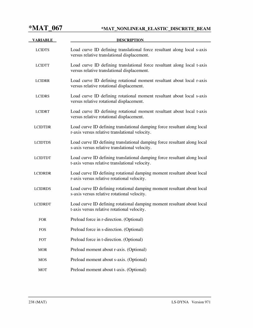
*MAT_067 *MAT_NONLINEAR_ELASTIC_DISCRETE_BEAM
238 (MAT) LS-DYNA Version 971
VARIABLE DESCRIPTION
LCIDTS Load curve ID defining translational force resultant along local s-axis versus relative translational displacement.
LCIDTT Load curve ID defining translational force resultant along local t-axis versus relative translational displacement.
LCIDRR Load curve ID defining rotational moment resultant about local r-axis versus relative rotational displacement.
LCIDRS Load curve ID defining rotational moment resultant about local s-axis versus relative rotational displacement.
LCIDRT Load curve ID defining rotational moment resultant about local t-axis versus relative rotational displacement.
LCIDTDR Load curve ID defining translational damping force resultant along local r-axis versus relative translational velocity.
LCIDTDS Load curve ID defining translational damping force resultant along local s-axis versus relative translational velocity.
LCIDTDT Load curve ID defining translational damping force resultant along local t-axis versus relative translational velocity.
LCIDRDR Load curve ID defining rotational damping moment resultant about local r-axis versus relative rotational velocity.
LCIDRDS Load curve ID defining rotational damping moment resultant about local s-axis versus relative rotational velocity.
LCIDRDT Load curve ID defining rotational damping moment resultant about local t-axis versus relative rotational velocity.
FOR Preload force in r-direction. (Optional)
FOS Preload force in s-direction. (Optional)
FOT Preload force in t-direction. (Optional)
MOR Preload moment about r-axis. (Optional)
MOS Preload moment about s-axis. (Optional)
MOT Preload moment about t-axis. (Optional)

*MAT_NONLINEAR_ELASTIC_DISCRETE_BEAM *MAT_067
LS-DYNA Version 971 239 (MAT)
Remarks:
For null load curve ID’s, no forces are computed.
The formulation of the discrete beam (type 6) assumes that the beam is of zero length and requires no orientation node. A small distance between the nodes joined by the beam is permitted. The local coordinate system which determines (r,s,t) is given by the coordinate ID, see *DEFINE_ COORDINATE_OPTION, in the cross sectional input, see *SECTION_BEAM, where the global system is the default. The local coordinate system axes can rotate with either node of the beam or an average rotation of both nodes (see SCOOR variable in *SECTION_BEAM).
If different behavior in tension and compression is desired in the calculation of the force resultants, the load curve(s) must be defined in the negative quadrant starting with the most negative displacement then increasing monotonically to the most positive. If the load curve behaves similarly in tension and compression, define only the positive quadrant. Whenever displacement values fall outside of the defined range, the resultant forces will be extrapolated. Figure 67.1 depicts a typical load curve for a force resultant. Load curves used for determining the damping forces and moment resultants always act identically in tension and compression, since only the positive quadrant values are considered, i.e., start the load curve at the origin [0,0].
Figure 67.1. The resultant forces and moments are determined by a table lookup. If the origin of the load curve is at [0,0] as in (b.) and tension and compression responses are symmetric.

*MAT_068 *MAT_NONLINEAR_PLASTIC_DISCRETE_BEAM
240 (MAT) LS-DYNA Version 971
*MAT_NONLINEAR_PLASTIC_DISCRETE_BEAM
This is Material Type 68. This material model is defined for simulating the effects of nonlinear elastoplastic, linear viscous behavior of beams by using six springs each acting about one of the six local degrees-of-freedom. The two nodes defining a beam may be coincident to give a zero length beam, or offset to give a finite length beam. For finite length discrete beams the absolute value of the variable SCOOR in the SECTION_BEAM input should be set to a value of 2.0, which causes the local r-axis to be aligned along the two nodes of the beam to give physically correct behavior. The distance between the nodes of a beam should not affect the behavior of this material model. A triad is used to orient the beam for the directional springs. Translational/rotational stiffness and damping effects can be considered. The plastic behavior is modeled using force/moment curves versus displacements/ rotation. Optionally, failure can be specified based on a force/moment criterion and a displacement/ rotation criterion. See also notes below.
Card 1 1 2 3 4 5 6 7 8
Variable MID RO TKR TKS TKT RKR RKS RKT
Type A8 F F F F F F F
Default none none none none none none none none
Card 2
Variable TDR TDS TDT RDR RDS RDT
Type F F F F F F
Default none none none none none none

*MAT_NONLINEAR_PLASTIC_DISCRETE_BEAM *MAT_068
LS-DYNA Version 971 241 (MAT)
Card 3 1 2 3 4 5 6 7 8
Variable LCPDR LCPDS LCPDT LCPMR LCPMS LCPMT
Type F F F F F F
Default 0.0 0.0 0.0 0.0 0.0 0.0
Card 4
Variable FFAILR FFAILS FFAILT MFAILR MFAILS MFAILT
Type F F F F F F
Default 0.0 0.0 0.0 0.0 0.0 0.0
Card 5
Variable UFAILR UFAILS UFAILT TFAILR TFAILS TFAILT
Type F F F F F F
Default 0.0 0.0 0.0 0.0 0.0 0.0
Card 6
Variable FOR FOS FOT MOR MOS MOT
Type F F F F F F
VARIABLE DESCRIPTION
MID Material identification. A unique number or label not exceeding 8 characters must be specified.
RO Mass density, see also volume on *SECTION_BEAM definition.

*MAT_068 *MAT_NONLINEAR_PLASTIC_DISCRETE_BEAM
242 (MAT) LS-DYNA Version 971
VARIABLE DESCRIPTION
TKR Translational stiffness about local r-axis
TKS Translational stiffness about local s-axis
TKT Translational stiffness about local t-axis
RKR Rotational stiffness about the local r-axis
RKS Rotational stiffness about the local s-axis
RKT Rotational stiffness about the local t-axis
TDR Translational viscous damper about local r-axis
TDS Translational viscous damper about local s-axis
TDT Translational viscous damper about local t-axis
RDR Rotational viscous damper about the local r-axis
RDS Rotational viscous damper about the local s-axis
RDT Rotational viscous damper about the local t-axis
LCPDR Load curve ID-yield force versus plastic displacement r-axis. If the curve ID is zero, and if TKR is nonzero, then elastic behavior is obtained for this component.
LCPDS Load curve ID-yield force versus plastic displacement s-axis. If the curve ID is zero, and if TKS is nonzero, then elastic behavior is obtained for this component.
LCPDT Load curve ID-yield force versus plastic displacement t-axis. If the curve ID is zero, and if TKT is nonzero, then elastic behavior is obtained for this component.
LCPMR Load curve ID-yield moment versus plastic rotation r-axis. If the curve ID is zero, and if RKR is nonzero, then elastic behavior is obtained for this component.
LCPMS Load curve ID-yield moment versus plastic rotation s-axis. If the curve ID is zero, and if RKS is nonzero, then elastic behavior is obtained for this component.
LCPMT Load curve ID-yield moment versus plastic rotation t-axis. If the curve ID is zero, and if RKT is nonzero, then elastic behavior is obtained for this component.

*MAT_NONLINEAR_PLASTIC_DISCRETE_BEAM *MAT_068
LS-DYNA Version 971 243 (MAT)
VARIABLE DESCRIPTION
FFAILR Optional failure parameter. If zero, the corresponding force, Fr, is not considered in the failure calculation.
FFAILS Optional failure parameter. If zero, the corresponding force, Fs, is not considered in the failure calculation.
FFAILT Optional failure parameter. If zero, the corresponding force, Ft, is not considered in the failure calculation.
MFAILR Optional failure parameter. If zero, the corresponding moment, Mr, is not considered in the failure calculation.
MFAILS Optional failure parameter. If zero, the corresponding moment, Ms, is not considered in the failure calculation.
MFAILT Optional failure parameter. If zero, the corresponding moment, Mt, is not considered in the failure calculation.
UFAILR Optional failure parameter. If zero, the corresponding displacement, ur,is not considered in the failure calculation.
UFAILS Optional failure parameter. If zero, the corresponding displacement, us,is not considered in the failure calculation.
UFAILT Optional failure parameter. If zero, the corresponding displacement, ut,is not considered in the failure calculation.
TFAILR Optional failure parameter. If zero, the corresponding rotation, θr, is not considered in the failure calculation.
TFAILS Optional failure parameter. If zero, the corresponding rotation, θs, is not considered in the failure calculation.
TFAILT Optional failure parameter. If zero, the corresponding rotation, θt, is not considered in the failure calculation.
FOR Preload force in r-direction. (Optional)
FOS Preload force in s-direction. (Optional)
FOT Preload force in t-direction. (Optional)
MOR Preload moment about r-axis. (Optional)
MOS Preload moment about s-axis. (Optional)
MOT Preload moment about t-axis. (Optional)

*MAT_068 *MAT_NONLINEAR_PLASTIC_DISCRETE_BEAM
244 (MAT) LS-DYNA Version 971
Remarks:
For the translational and rotational degrees of freedom where elastic behavior is desired, set the load curve ID to zero.
The formulation of the discrete beam (type 6) assumes that the beam is of zero length and requires no orientation node. A small distance between the nodes joined by the beam is permitted. The local coordinate system which determines (r,s,t) is given by the coordinate ID (see *DEFINE_COORDINATE_OPTION) in the cross sectional input, see *SECTION_BEAM, where the global system is the default. The local coordinate system axes can rotate with either node of the beam or an average rotation of both nodes (see SCOOR variable in *SECTION_BEAM).
Catastrophic failure based on force resultants occurs if the following inequality is satisfied.
2 2 2 22 2
1. 0.r s t r s tfail fail fail fail fail fail
r s t r s t
F F F M M M
F F F M M M+ + + + + − ≥
After failure the discrete element is deleted. Likewise, catastrophic failure based on displacement resultants occurs if the following inequality is satisfied:
2 2 2 22 2
1. 0.r s t r s tfail fail fail fail fail fail
r s t r s t
u u u
u u u
θ θ θθ θ θ
+ + + + + − ≥
After failure the discrete element is deleted. If failure is included either one or both of the criteria may be used.
Figure 68.1. The resultant forces and moments are limited by the yield definition. The initial yield point corresponds to a plastic displacement of zero.

*MAT_SID_DAMPER_DISCRETE_BEAM *MAT_069
LS-DYNA Version 971 245 (MAT)
*MAT_SID_DAMPER_DISCRETE_BEAM
This is Material Type 69. The side impact dummy uses a damper that is not adequately treated by the nonlinear force versus relative velocity curves since the force characteristics are dependent on the displacement of the piston. See also notes below.
Card 1 1 2 3 4 5 6 7 8
Variable MID RO ST D R H K C
Type A8 F F F F F F F
Card 2
Variable C3 STF RHOF C1 C2 LCIDF LCIDD S0
Type F F F F F F F F
Read in up to 15 orifice locations with orifice location per card. Input is terminated when a “*” card is found. On the first card below the optional input parameters SF and DF may be specified.
Cards 3... 1 2 3 4 5 6 7 8
Variable ORFLOC ORFRAD SF DC
Type F F F F
VARIABLE DESCRIPTION
MID Material identification. A unique number or label not exceeding 8 characters must be specified.
RO Mass density, see also volume on *SECTION_BEAM definition.
ST St, piston stroke. St must equal or exceed the length of the beam element, see Figure 69.1 below.
D d, piston diameter

*MAT_069 *MAT_SID_DAMPER_DISCRETE_BEAM
246 (MAT) LS-DYNA Version 971
VARIABLE DESCRIPTION
R R, default orifice radius
H h, orifice controller position
K K, damping constant
LT.0.0: |K| is the load curve number ID, see *DEFINE_CURVE, defining the damping coefficient as a function of the absolute value of the relative velocity.
C C, discharge coefficient
C3 Coefficient for fluid inertia term
STF k, stiffness coefficient if piston bottoms out
RHOF fluid , fluid density
C1 C1, coefficient for linear velocity term
C2 C2, coefficient for quadratic velocity term
LCIDF Load curve number ID defining force versus piston displacement, s, i.e., term ( )0f s s+ . Compressive behavior is defined in the positive
quadrant of the force displacement curve. Displacements falling outside of the defined force displacement curve are extrapolated. Care must be taken to ensure that extrapolated values are reasonable.
LCIDD Load curve number ID defining damping coefficient versus piston displacement, s, i.e., ( )0g s s+ . Displacements falling outside the
defined curve are extrapolated. Care must be taken to ensure that extrapolated values are reasonable.
S0 Initial displacement s0, typically set to zero. A positive displacement corresponds to compressive behavior.
ORFLOC di, orifice location of ith orifice relative to the fixed end.
ORFRAD ri, orifice radius of ith orifice, if zero the default radius is used.
SF Scale factor on calculated force. The default is set to 1.0
DC c, linear viscous damping coefficient used after damper bottoms out either in tension or compression.

*MAT_SID_DAMPER_DISCRETE_BEAM *MAT_069
LS-DYNA Version 971 247 (MAT)
Remarks:
As the damper moves, the fluid flows through the open orifices to provide the necessary damping resistance. While moving as shown in Figure 69.1 the piston gradually blocks off and effectively closes the orifices. The number of orifices and the size of their opening control the damper resistance and performance. The damping force is computed from,
( ) ( )2
12 0 0
0 0
1pp p p fluid pt t
ACF SF KA V C V f s s V g s s
A CAρ= + − − + + +
where K is a user defined constant or a tabulated function of the absolute value of the relative velocity, Vp is the piston velocity, C is the discharge coefficient, Ap is the piston area, 0
tA is the
total open areas of orifices at time t, ρfluid is the fluid density, C1 is the coefficient for the linear term, and C2 is the coefficient for the quadratic term.
In the implementation, the orifices are assumed to be circular with partial covering by the orifice controller. As the piston closes, the closure of the orifice is gradual. This gradual closure is properly taken into account to insure a smooth response. If the piston stroke is exceeded, the stiffness value, k, limits further movement, i.e., if the damper bottoms out in tension or compression the damper forces are calculated by replacing the damper by a bottoming out spring and damper, k and c, respectively. The piston stroke must exceed the initial length of the beam element. The time step calculation is based in part on the stiffness value of the bottoming out spring. A typical force versus displacement curve at constant relative velocity is shown in Figure 69.2.
The factor, SF, which scales the force defaults to 1.0 and is analogous to the adjusting ring on the damper.

*MAT_069 *MAT_SID_DAMPER_DISCRETE_BEAM
248 (MAT) LS-DYNA Version 971
Figure 69.1. Mathematical model for the Side Impact Dummy damper.
Figure 69.2. Force versus displacement as orifices are covered at a constant relative velocity. Only the linear velocity term is active.

*MAT_HYDRAULIC_GAS_DAMPER_DISCRETE_BEAM *MAT_070
LS-DYNA Version 971 249 (MAT)
*MAT_HYDRAULIC_GAS_DAMPER_DISCRETE_BEAM
This is Material Type 70. This special purpose element represents a combined hydraulic and gas-filled damper which has a variable orifice coefficient. A schematic of the damper is shown in Figure 70.1. Dampers of this type are sometimes used on buffers at the end of railroad tracks and as aircraft undercarriage shock absorbers. This material can be used only as a discrete beam element. See also notes below.
Card 1 1 2 3 4 5 6 7 8
Variable MID RO CO N P0 PA AP KH
Type A8 F F F F F F F
Card 2
Variable LCID FR SCLF CLEAR
Type F F F F
VARIABLE DESCRIPTION
MID Material identification. A unique number or label not exceeding 8 characters must be specified.
RO Mass density, see also volume in *SECTION_BEAM definition.
CO Length of gas column, Co
N Adiabatic constant
P0 Initial gas pressure, P0
PA Atmospheric pressure, Pa
AP Piston cross sectional area, Ap
KH Hydraulic constant, K
LCID Load curve ID, see *DEFINE_CURVE, defining the orifice area, a0,versus element deflection.

*MAT_070 *MAT_HYDRAULIC_GAS_DAMPER_DISCRETE_BEAM
250 (MAT) LS-DYNA Version 971
VARIABLE DESCRIPTION
FR Return factor on orifice force. This acts as a factor on the hydraulic force only and is applied when unloading. It is intended to represent a valve that opens when the piston unloads to relieve hydraulic pressure. Set it to 1.0 for no such relief.
SCLF Scale factor on force. (Default = 1.0)
CLEAR Clearance (if nonzero, no tensile force develops for positive displacements and negative forces develop only after the clearance is closed.
Figure 70.1. Schematic of Hydraulic/Gas damper.
Remarks:
As the damper is compressed two actions contribute to the force which develops. First, the gas is adiabatically compressed into a smaller volume. Secondly, oil is forced through an orifice. A profiled pin may occupy some of the cross-sectional area of the orifice; thus, the orifice area available for the oil varies with the stroke. The force is assumed proportional to the square of the velocity and inversely proportional to the available area.
The equation for this element is:
2
00
0 0
n
h a p
V CF SCLF K P P A
a C S= ⋅ + − ⋅
−
where S is the element deflection and V is the relative velocity across the element.

*MAT_CABLE_DISCRETE_BEAM *MAT_071
LS-DYNA Version 971 251 (MAT)
*MAT_CABLE_DISCRETE_BEAM
This is Material Type 71. This model permits elastic cables to be realistically modeled; thus, no force will develop in compression.
Note: The following options will be available starting in release 3 of version 971: TMAXF0,TRAMP, IREAD, OUTPUT.
Card 1 1 2 3 4 5 6 7 8
Variable MID RO E LCID F0 TMAXF0 TRAMP IREAD
Type A8 F F F F F F I
Default none none none none 0 0 0 0
Define Card 2 only if IREAD > 0
Card 2 1 2 3 4 5 6 7 8
Variable OUTPUT
Type I
Default 0
VARIABLE DESCRIPTION
MID Material identification. A unique number or label not exceeding 8 characters must be specified.
RO Mass density, see also volume in *SECTION_BEAM definition.
E GT.0.0: Young's modulus LT.0.0: Stiffness
LCID Load curve ID, see *DEFINE_CURVE, defining the stress versus engineering strain. (Optional).
F0 Initial tensile force. If F0 is defined, an offset is not needed for an initial tensile force.

*MAT_071 *MAT_CABLE_DISCRETE_BEAM
252 (MAT) LS-DYNA Version 971
VARIABLE DESCRIPTION
TMAXF0 Time for which pre-tension force will be held
TRAMP Ramp-up time for pre-tension force
OUTPUT Flag =1 to output axial strain (see note)
Remarks:
The force, F, generated by the cable is nonzero if and only if the cable is tension. The force is given by:
( )0max ,0.F F K L= + Δ
where LΔ is the change in length
( )L current length initial length offsetΔ = − −
and the stiffness (E > 0.0 only ) is defined as:
( )E area
Kinitial length offset
⋅=−
Note that a constant force element can be obtained by setting:
0 0 0F and K> =
although the application of such an element is unknown.
The area and offset are defined on either the cross section or element cards. For a slack cable the offset should be input as a negative length. For an initial tensile force the offset should be positive.
If a load curve is specified the Young’s modulus will be ignored and the load curve will be used instead. The points on the load curve are defined as engineering stress versus engineering strain, i.e., the change in length over the initial length. The unloading behavior follows the loading.
By default, cable pretension is applied only at the start of the analysis. If the cable is attached to flexible structure, deformation of the structure will result in relaxation of the cables, which will therefore lose some or all of the intended preload.
This can be overcome by using TMAXF0. In this case, it is expected that the structure will deform under the loading from the cables and that this deformation will take time to occur during the analysis. The unstressed length of the cable will be continuously adjusted until time TMAXF0 such that the force is maintained at the user-defined pre-tension force – this is
*MAT_CABLE_DISCRETE_BEAM *MAT_071
LS-DYNA Version 971 253 (MAT)
analogous to operation of the pre-tensioning screws in real cables. After time TMAXF0, the unstressed length is fixed and the force in the cable is determined in the normal way using the stiffness and change of length.
Sudden application of the cable forces at time zero may result in an excessively dynamic response during pre-tensioning. A ramp-up time TRAMP may optionally be defined. The cable force ramps up from zero at time zero to the full pre-tension F0 at time TRAMP. TRAMP should be less than or equal to TMAXF0.
If the model does not use dynamic relaxation, it is recommended that damping be applied during pre-tensioning so that the structure reaches a steady state by time TMAXF0.
If the model uses dynamic relaxation, TRAMP applies only during dynamic relaxation. The preload is held constant until the end of dynamic relaxation. The full cable pre-tension is retained after convergence, and TMAXF0 applies during the subsequent transient analysis. TMAXF0 can in this case be set to zero if required.
The cable mass will be calculated from length x area x density if VOL is set to zero on *SECTION_BEAM. Otherwise, VOL x density will be used.
If OUTPUT is set in any cable material, extra variables will be written to the d3plot and d3thdt files for all beam elements. Post-processors should interpret the extra data as per Resultant beams. Only the first extra data item, axial strain, is computed for MAT_CABLE elements.
If the stress-strain load curve option, LCID, is combined with preload, two types of behavior are available:
1. If the preload is applied using the TMAXF0/TRAMP method, the initial strain is calculated from the stress-strain curve to achieve the desired preload.
2. If TMAXF0/TRAMP are not used, the preload force is taken as additional to the force calculated from the stress/strain curve. Thus, the total stress in the cable will be higher than indicated by the stress/strain curve.

*MAT_072 *MAT_CONCRETE_DAMAGE
254 (MAT) LS-DYNA Version 971
*MAT_CONCRETE_DAMAGE
This is Material Type 72. This model has been used to analyze buried steel reinforced concrete structures subjected to impulsive loadings. A newer version of this model is available as *MAT_ CONCRETE_DAMAGE_REL3
Card 1 1 2 3 4 5 6 7 8
Variable MID RO PR
Type A8 F F
Default none none none
Card 2
Variable SIGF A0 A1 A2
Type F F F F
Default 0.0 0.0 0.0 0.0
Card 3
Variable A0Y A1Y A2Y A1F A2F B1 B2 B3
Type F F F F F F F F
Default 0.0 0.0 0.0 0.0 0.0 0.0 0.0 0.0

*MAT_CONCRETE_DAMAGE *MAT_072
LS-DYNA Version 971 255 (MAT)
Card 4 1 2 3 4 5 6 7 8
Variable PER ER PRR SIGY ETAN LCP LCR
Type F F F F F F F
Default 0.0 0.0 0.0 none 0.0 none none
Card 5
Variable λ λ2 λ3 λ4 λ5 λ6 λ7 λ8
Type F F F F F F F F
Default none none none none none none none none
Card 6
Variable λ9 λ10 λ11 λ12 λ13
Type F F F F F
Default none none none none none
Card 7
Variable η1 η2 η3 η4 η5 η6 η7 η8
Type F F F F F F F F
Default none none none none none none none none

*MAT_072 *MAT_CONCRETE_DAMAGE
256 (MAT) LS-DYNA Version 971
Card 8 1 2 3 4 5 6 7 8
Variable η9 η10 η11 η12 η13
Type F F F F F
Default none none none none none
VARIABLE DESCRIPTION
MID Material identification. A unique number or label not exceeding 8 characters must be specified.
RO Mass density.
PR Poisson’s ratio.
SIGF Maximum principal stress for failure.
A0 Cohesion.
A1 Pressure hardening coefficient.
A2 Pressure hardening coefficient.
A0Y Cohesion for yield
A1Y Pressure hardening coefficient for yield limit
A2Y Pressure hardening coefficient for yield limit
A1F Pressure hardening coefficient for failed material.
A2F Pressure hardening coefficient for failed material.
B1 Damage scaling factor.
B2 Damage scaling factor for uniaxial tensile path.
B3 Damage scaling factor for triaxial tensile path.
PER Percent reinforcement.
ER Elastic modulus for reinforcement.

*MAT_CONCRETE_DAMAGE *MAT_072
LS-DYNA Version 971 257 (MAT)
VARIABLE DESCRIPTION
PRR Poisson’s ratio for reinforcement.
SIGY Initial yield stress.
ETAN Tangent modulus/plastic hardening modulus.
LCP Load curve ID giving rate sensitivity for principal material, see *DEFINE_CURVE.
LCR Load curve ID giving rate sensitivity for reinforcement, see *DEFINE_CURVE.
λ1-λ13 Tabulated damage function
η1-η13 Tabulated scale factor.
Remarks: Cohesion for failed material a0f = 0.0
B3 must be positive or zero. λn < λn+1. The first point must be zero.

*MAT_072R3 *MAT_CONCRETE_DAMAGE_REL3
258 (MAT) LS-DYNA Version 971
*MAT_CONCRETE_DAMAGE_REL3
This is Material Type 72. The Karagozian & Case (K&C) Concrete Model - Release III is a three-invariant model, uses three shear failure surfaces, includes damage and strain-rate effects, and has origins based on the Pseudo-TENSOR Model (Material Type 16). The most significant user improvement provided by Release III is a model parameter generation capability, based solely on the unconfined compression strength of the concrete. The implementation of Release III significantly changed the user input, thus previous input files using Material Type 72, i.e. prior to LS-DYNA Version 971, are not compatible with the present input format.
An open source reference, that precedes the parameter generation capability, is provided in Malvar et al. [1997]. A workshop proceedings reference, Malvar et al. [1996], is useful, but may be difficult to obtain. More recent, but limited distribution reference materials, e.g. Malvar et al. [2000], may be obtained by contacting Karagozian & Case.
Seven card images are required to define the complete set of model parameters for the K&C Concrete Model; an Equation-of-State is also required for the pressure-volume strain response. Brief descriptions of all the input parameters are provided below, however it is expected that this model will be used primarily with the option to generate the model parameters based on the unconfined compression strength of the concrete. For those users wishing to examine, or modify, the generated model parameters, the generated parameters are written to the LS-DYNA messagfile (FORTRAN Unit 59). The pressure-volume strain response for the model is also generated, in the form of a Tabulated Compaction Equation-of-State (EOS 8) whose parameters are also written to the LS-DYNA “messag” file.
Card 1 1 2 3 4 5 6 7 8
Variable MID RO PR
Type A8 F F
Default none none none
Card 2
Variable FT A0 A1 A2 B1 OMEGA A1F
Type F F F F F F F
Default 0.0 0.0 0.0 0.0 0.0

*MAT_CONCRETE_DAMAGE_REL3 *MAT_072R3
LS-DYNA Version 971 259 (MAT)
Card 3 1 2 3 4 5 6 7 8
Variable Sλ NOUT EDROP RSIZE UCF LCRATE LOCWID NPTS
Type F F F F F F F F
Default
Card 4
Variable λ01 λ02 λ03 λ04 λ05 λ06 λ07 λ08
Type F F F F F F F F
Default none none none none none none none none
Card 5
Variable λ09 λ10 λ11 λ12 λ13 B3 A0Y A1Y
Type F F F F F F F F
Default none none none none none none 0.0 0.0
Card 6
Variable η01 η02 η03 η04 η05 η06 η07 η08
Type F F F F F F F F
Default none none none none none none none none

*MAT_072R3 *MAT_CONCRETE_DAMAGE_REL3
260 (MAT) LS-DYNA Version 971
Card 7 1 2 3 4 5 6 7 8
Variable η09 η10 η11 η12 η13 B2 A2F A2Y
Type F F F F F F F F
Default none none none none none 0.0 0.0 0.0
VARIABLE DESCRIPTION
MID Material identification. A unique number or label not exceeding 8 characters must be specified.
RO Mass density.
PR Poisson’s ratio, v .
FT Uniaxial tensile strength, tf .
A0 Maximum shear failure surface parameter, 0a or cf ′− for parameter generation (recommended).
A1 Maximum shear failure surface parameter, 1a .
A2 Maximum shear failure surface parameter, 2a .
B1 Compressive damage scaling parameter, 1b
OMEGA Fractional dilatancy, ω .
A1F Residual failure surface coefficient, 1 fa .
Sλ λ stretch factor, s.
NOUT Output selector for effective plastic strain (see table).
EDROP Post peak dilatancy decay, N α .
RSIZE Unit conversion factor for length (inches/user-unit), e.g. 39.37 if user length unit in meters.
UCF Unit conversion factor for stress (psi/user-unit), e.g. 145 if cf ′ in MPa.

*MAT_CONCRETE_DAMAGE_REL3 *MAT_072R3
LS-DYNA Version 971 261 (MAT)
VARIABLE DESCRIPTION
LCRATE Define (load) curve number for strain-rate effects; effective strain rate on abscissa and strength enhancement on ordinate.
LOCWID Three times the maximum aggregate diameter (input in user length units).
NPTS Number of points in λ versusη damage relation; must be 13 points.
λ01 1st value of damage function, 1λ
λ02 2nd value of damage function,
λ03 3rd value of damage function,
λ04 4th value of damage function,
λ05 5th value of damage function,
λ06 6th value of damage function,
λ07 7th value of damage function,
λ08 8th value of damage function, 8λ
λ09 9th value of damage function,
λ10 10th value of damage function,
λ11 11th value of damage function,
λ12 12th value of damage function,
λ13 13th value of damage function, 13λ .
B3 Damage scaling coefficient for triaxial tension, 3b .
A0Y Initial yield surface cohesion, 0 ya .
A1Y Initial yield surface coefficient, 1ya .
η01 1st value of scale factor, 1η .
η02 2nd value of scale factor,
η03 3rd value of scale factor,

*MAT_072R3 *MAT_CONCRETE_DAMAGE_REL3
262 (MAT) LS-DYNA Version 971
VARIABLE DESCRIPTION
η04 4th value of scale factor,
η05 5th value of scale factor,
η06 6th value of scale factor,
η07 7th value of scale factor,
η08 8th value of scale factor, 8η
η09 9th value of scale factor, 9η
η10 10th value of scale factor,
η11 11th value of scale factor,
η12 12th value of scale factor,
η13 13th value of scale factor, 13η .
B2 Tensile damage scaling exponent, 2b .
A2F Residual failure surface coefficient, 2 fa .
A2Y Initial yield surface coefficient, 2 ya .

*MAT_CONCRETE_DAMAGE_REL3 *MAT_072R3
LS-DYNA Version 971 263 (MAT)
Output of Selected Variables
LS-PrePost will display the variable described in Table 72.1 when the effective plastic strain is selected, for the corresponding user input value of NOUT; see Card 3 above.
Table 72.1 Output variables for post-processing using NOUT parameter.
NOUT Function Description 1 Current shear failure surface radius
2 ( )2 / mδ λ λ λ= + Scaled damage measure
3 ij ijσ ε Strain energy (rate)
4 pij ijσ ε Plastic strain energy (rate)
Sample Input for Concrete
As an example of the K&C Concrete Model material parameter generation, the following sample input for a 45.4 MPa (6,580 psi) unconfined compression strength concrete is provided. The basic units for the provided parameters are length in millimeters (mm), time in milliseconds (msec), and mass in grams (g). This base unit set yields units of force in Newtons (N) and pressure in Mega-Pascals (MPa).
Card 1 1 2 3 4 5 6 7 8
Variable MID RO PR
Type 72 2.3E-3
Card 2
Variable FT A0 A1 A2 B1 OMEGA A1F
Type F -45.4

*MAT_072R3 *MAT_CONCRETE_DAMAGE_REL3
264 (MAT) LS-DYNA Version 971
Card 3 1 2 3 4 5 6 7 8
Variable Sλ NOUT EDROP RSIZE UCF LCRATE LOCWID NPTS
Type 3.94E-2 145.0 723.0
Card 4
Variable λ01 λ02 λ03 λ04 λ05 λ06 λ07 λ08
Type
Card 5
Variable λ09 λ10 λ11 λ12 λ13 B3 A0Y A1Y
Type
Card 6
Variable η01 η02 η03 η04 η05 η06 η07 η08
Type
Card 7
Variable η09 η10 η11 η12 η13 B2 A2F A2Y
Type
The effective strain rate versus shear strength enhancement is given by a LS-DYNA Define (load) Curve keyword, with ID 723. The sample input values, see Malvar & Ross [1998], are given in Table 72.2.

*MAT_CONCRETE_DAMAGE_REL3 *MAT_072R3
LS-DYNA Version 971 265 (MAT)
Table 72.2 Effective strain rate for 45.4 MPa concrete MAT 72 sample input.
Strain-Rate (1/ms) Enhancement -3.0E+01 9.70 -3.0E-01 9.70 -1.0E-01 6.72 -3.0E-02 4.50 -1.0E-02 3.12 -3.0E-03 2.09 -1.0E-03 1.45 -1.0E-04 1.36 -1.0E-05 1.28 -1.0E-06 1.20 -1.0E-07 1.13 -1.0E-08 1.06 0.0E+00 1.00 3.0E-08 1.00 1.0E-07 1.03 1.0E-06 1.08 1.0E-05 1.14 1.0E-04 1.20 1.0E-03 1.26 3.0E-03 1.29 1.0E-02 1.33 3.0E-02 1.36 1.0E-01 2.04 3.0E-01 2.94 3.0E+01 2.94

*MAT_073 *MAT_LOW_DENSITY_VISCOUS_FOAM
266 (MAT) LS-DYNA Version 971
*MAT_LOW_DENSITY_VISCOUS_FOAM
This is Material Type 73 for Modeling Low Density Urethane Foam with high compressibility and with rate sensitivity which can be characterized by a relaxation curve. Its main applications are for seat cushions, padding on the Side Impact Dummies (SID), bumpers, and interior foams. Optionally, a tension cut-off failure can be defined. Also, see the notes below and the description of material 57: *MAT_LOW_DENSITY_FOAM.
Card 1 1 2 3 4 5 6 7 8
Variable MID RO E LCID TC HU BETA DAMP
Type A8 F F F F F F F
Default --- --- --- --- 1.E+20 1.
Remarks --- --- --- --- --- 3 1 ---
Card 2
Variable SHAPE FAIL BVFLAG KCON LCID2 BSTART TRAMP NV
Type F F F F F F F I
Default 1.0 0.0 0.0 0.0 0 0.0 0.0 6

*MAT_LOW_DENSITY_VISCOUS_FOAM *MAT_073
LS-DYNA Version 971 267 (MAT)
If LCID2 = 0 then define the following viscoelastic constants. Up to 6 cards may be input. A keyword card (with a “*” in column 1) terminates this input if less than 6 cards are used. If LCID2 is nonzero skip this input. The variable REF is taken from the first card of this sequence.
Optional Cards
1 2 3 4 5 6 7 8
Variable GI BETAI REF
Type F F F
VARIABLE DESCRIPTION
MID Material identification. A unique number or label not exceeding 8 characters must be specified.
RO Mass density
E Young’s modulus used in tension. For implicit problems E is set to the initial slope of load curve LCID.
LCID Load curve ID, see *DEFINE_CURVE, for nominal stress versus strain.
TC Tension cut-off stress
HU Hysteretic unloading factor between 0 and 1 (default=1, i.e., no energy dissipation), see also Figure 57.1.
BETA β, decay constant to model creep in unloading. EQ:0 No relaxation.
DAMP Viscous coefficient (.05< recommended value <.50) to model damping effects.
LT.0.0: |DAMP| is the load curve ID, which defines the damping constant as a function of the maximum strain in compression defined as:
( )max 1 2 3max 1 ,1 ,1.ε λ λ λ= − − − .
In tension, the damping constant is set to the value corresponding to the strain at 0. The abscissa should be defined from 0 to 1.
SHAPE Shape factor for unloading. Active for nonzero values of the hysteretic unloading factor. Values less than one reduces the energy dissipation and greater than one increases dissipation, see also Figure 57.1.

*MAT_073 *MAT_LOW_DENSITY_VISCOUS_FOAM
268 (MAT) LS-DYNA Version 971
VARIABLE DESCRIPTION
FAIL Failure option after cutoff stress is reached: EQ.0.0: tensile stress remains at cut-off value, EQ.1.0: tensile stress is reset to zero.
BVFLAG Bulk viscosity activation flag, see remark below: EQ.0.0: no bulk viscosity (recommended), EQ.1.0: bulk viscosity active.
KCON Stiffness coefficient for contact interface stiffness. Maximum slope in stress vs. strain curve is used. When the maximum slope is taken for the contact, the time step size for this material is reduced for stability. In some cases Δt may be significantly smaller, and defining a reasonable stiffness is recommended.
LCID2 Load curve ID of relaxation curve. If constants βι are determined via a least squares fit. This relaxation curve is shown in Figure 76.1. This model ignores the constant stress.
BSTART Fit parameter. In the fit, β1 is set to zero, β2 is set to BSTART, β3 is 10 times β2, β4 is 10 times greater than β3 , and so on. If zero, BSTART= .01.
TRAMP Optional ramp time for loading.
NV Number of terms in fit. If zero, the default is 6. Currently, the maximum number is set to 6. Values of 2 are 3 are recommended, since each term used adds significantly to the cost. Caution should be exercised when taking the results from the fit. Preferably, all generated coefficients should be positive. Negative values may lead to unstable results. Once a satisfactory fit has been achieved it is recommended that the coefficients which are written into the output file be input in future runs.
GI Optional shear relaxation modulus for the ith term
BETAI Optional decay constant if ith term
REF Use reference geometry to initialize the stress tensor. The reference geometry is defined by the keyword:*INITIAL_FOAM_REFERENCE_ GEOMETRY (see there for more details).
EQ.0.0: off, EQ.1.0: on.

*MAT_LOW_DENSITY_VISCOUS_FOAM *MAT_073
LS-DYNA Version 971 269 (MAT)
Remarks:
This viscoelastic foam model is available to model highly compressible viscous foams. The hyperelastic formulation of this model follows that of Material 57.
Rate effects are accounted for through linear viscoelasticity by a convolution integral of the form
( )0
tr klij ijklg t d
εσ τ ττ
∂= −∂
where ( )ijklg t τ− is the relaxation function. The stress tensor, rijσ , augments the stresses
determined from the foam, fijσ ; consequently, the final stress, ijσ , is taken as the summation of
the two contributions:
f rij ij ijσ σ σ= + .
Since we wish to include only simple rate effects, the relaxation function is represented by up to six terms of the Prony series:
( ) 01
Nt
mm
g t e βα α −
=
= +
This model is effectively a Maxwell fluid which consists of a dampers and springs in series. The formulation is performed in the local system of principal stretches where only the principal values of stress are computed and triaxial coupling is avoided. Consequently, the one-dimensional nature of this foam material is unaffected by this addition of rate effects. The addition of rate effects necessitates 42 additional history variables per integration point. The cost and memory overhead of this model comes primarily from the need to “remember” the local system of principal stretches and the evaluation of the viscous stress components.
Additional Remarks:
1. When hysteretic unloading is used the reloading will follow the unloading curve if the decay constant, β, is set to zero. If β is nonzero the decay to the original loading curve is governed by the expression:
1 te β−−
2. The bulk viscosity, which generates a rate dependent pressure, may cause an unexpected volumetric response and, consequently, it is optional with this model.
3. The hysteretic unloading factor results in the unloading curve to lie beneath the loading curve as shown in Figure 57.1. This unloading provides energy dissipation which is reasonable in certain kinds of foam.

*MAT_074 *MAT_ELASTIC_SPRING_DISCRETE_BEAM
270 (MAT) LS-DYNA Version 971
*MAT_ELASTIC_SPRING_DISCRETE_BEAM
This is Material Type 74. This model permits elastic springs with damping to be combined and represented with a discrete beam element type 6. Linear stiffness and damping coefficients can be defined, and, for nonlinear behavior, a force versus deflection and force versus rate curves can be used. Displacement based failure and an initial force are optional.
Card 1 1 2 3 4 5 6 7 8
Variable MID RO K F0 D CDF TDF
Type A8 F F F F F F
Card 2
Variable FLCID HLCID C1 C2 DLE GLCID
Type F F F F F I
VARIABLE DESCRIPTION
MID Material identification. A unique number or label not exceeding 8 characters must be specified.
RO Mass density, see also volume in *SECTION_BEAM definition.
K Stiffness coefficient.
F0 Optional initial force. This option is inactive if this material is referenced in a part referenced by material type *MAT_ELASTIC_ 6DOF_SPRING
D Viscous damping coefficient.
CDF Compressive displacement at failure. Input as a positive number. After failure, no forces are carried. This option does not apply to zero length springs.
EQ.0.0: inactive.
TDF Tensile displacement at failure. After failure, no forces are carried.
FLCID Load curve ID, see *DEFINE_CURVE, defining force versus deflection for nonlinear behavior.

*MAT_ELASTIC_SPRING_DISCRETE_BEAM *MAT_074
LS-DYNA Version 971 271 (MAT)
VARIABLE DESCRIPTION
HLCID Load curve ID, see *DEFINE_CURVE, defining force versus relative velocity for nonlinear behavior (optional). If the origin of the curve is at (0,0) the force magnitude is identical for a given magnitude of the relative velocity, i.e., only the sign changes.
C1 Damping coefficient for nonlinear behavior (optional).
C2 Damping coefficient for nonlinear behavior (optional).
DLE Factor to scale time units. The default is unity.
GLCID Optional load curve ID, see *DEFINE_CURVE, defining a scale factor versus deflection for load curve ID, HLCID. If zero, a scale factor of unity is assumed.
Remarks:
If the linear spring stiffness is used, the force, F, is given by:
0F F K L D L= + Δ + Δ
but if the load curve ID is specified, the force is then given by:
( ) ( ) ( ) ( )0 1 1 2 sgn ln max 1.,L
F F Kf L C L C L D L g L h LDLE
Δ= + Δ + ⋅ Δ + ⋅ Δ + Δ + Δ Δ
In these equations, LΔ is the change in length
L current length initial lengthΔ = −
The cross sectional area is defined on the section card for the discrete beam elements, See *SECTION_BEAM. The square root of this area is used as the contact thickness offset if these elements are included in the contact treatment.

*MAT_075 *MAT_BILKHU/DUBOIS_FOAM
272 (MAT) LS-DYNA Version 971
*MAT_BILKHU/DUBOIS_FOAM
This is Material Type 75. This model is for the simulation of isotropic crushable forms. Uniaxial and triaxial test data are used to describe the behavior.
Card 1 1 2 3 4 5 6 7 8
Variable MID RO YM LCPY LCUYS VC PC VPC
Type A8 F F F F F F F
Card 2
Variable TSC VTSC LCRATE PR KCON ISFLG
Type I F F F F F
VARIABLE DESCRIPTION
MID Material identification. A unique number or label not exceeding 8 characters must be specified.
RO Mass density
YM Young’s modulus (E)
LCPY Load curve ID giving pressure for plastic yielding versus volumetric strain, see Figure 75.1.
LCUYS Load curve ID giving uniaxial yield stress versus volumetric strain, see Figure 75.1, all abscissa should be positive if only the results of a compression test are included, optionally the results of a tensile test can be added (corresponding to negative values of the volumetric strain), in the latter case PC, VPC, TC and VTC will be ignored
VC Viscous damping coefficient (.05<recommended value<.50).
PC Pressure cutoff. If zero, the default is set to one-tenth of p0, the yield pressure corresponding to a volumetric strain of zero.
VPC Variable pressure cutoff as a fraction of pressure yield value. If non-zero this will override the pressure cutoff value PC.

*MAT_BILKHU/DUBOIS_FOAM *MAT_075
LS-DYNA Version 971 273 (MAT)
VARIABLE DESCRIPTION
TC Tension cutoff for uniaxial tensile stress. Default is zero. A nonzero value is recommended for better stability.
VTC Variable tension cutoff as a fraction of the uniaxial compressive yield strength, if non-zero this will override the tension cutoff value TC.
LCRATE Load curve ID giving a scale factor for the previous yield curves, dependent upon the volumetric plastic strain.
PR Poisson coefficient, which applies to both elastic and plastic deformations, must be smaller then 0.5
KCON Stiffness coefficient for contact interface stiffness. If undefined one-third of Young’s modulus, YM, is used. KCON is also considered in the element time step calculation; therefore, large values may reduce the element time step size.
ISFLG Flag for tensile response (active only if negative abscissa are present in load curve LCUYS)
EQ.0: load curve abscissa in tensile region correspond to volumetric strain
EQ.1: load curve abscissa in tensile region correspond to effective strain
Remarks:
The logarithmic volumetric strain is defined in terms of the relative volume, V , as:
( )ln Vγ = −
If used (ISFLG-1), the effective strain is defined in the usual way:
2:
3effε =
In defining the load curve LCPY the stress and strain pairs should be positive values starting with a volumetric strain value of zero.
The load curve LCUYS can optionally contain the results of the tensile test (corresponding to negative values of the volumetric strain), if so, then the load curve information will override PC, VPC, TC and VTC

*MAT_075 *MAT_BILKHU/DUBOIS_FOAM
274 (MAT) LS-DYNA Version 971
Figure 75.1. Behavior of crushable foam. Unloading is elastic.
The yield surface is defined as an ellipse in the equivalent pressure and von Mises stress plane.

*MAT_GENERAL_VISCOELASTIC *MAT_076
LS-DYNA Version 971 275 (MAT)
*MAT_GENERAL_VISCOELASTIC
This is Material Type 76. This material model provides a general viscoelastic Maxwell model having up to 6 terms in the prony series expansion and is useful for modeling dense continuum rubbers and solid explosives. Either the coefficients of the prony series expansion or a relaxation curve may be specified to define the viscoelastic deviatoric and bulk behavior.
The material model can also be used with laminated shell. Either an elastic or viscoelastic layer can be defined with the laminated formulation. To activate laminated shell you need the laminated formulation flag on *CONTROL_SHELL. With the laminated option a userdefined integration rule is needed.
Card 1 1 2 3 4 5 6 7 8
Variable MID RO BULK PCF EF TREF A B
Type A8 F F F F F F F
Insert a blank card here if constants are defined on cards 3,4,... below.
If an elastic layer is defined in a laminated shell this card must be blank.
Card 2 1 2 3 4 5 6 7 8
Variable LCID NT BSTART TRAMP LCIDK NTK BSTARTK TRAMPK
Type F I F F F I F F
Card Format for viscoelastic constants. Up to 6 cards may be input. A keyword card (with a “*” in column 1) terminates this input if less than 6 cards are used. These cards are not needed if relaxation data is defined. The number of terms for the shear behavior may differ from that for the bulk behavior: simply insert zero if a term is not included.
If an elastic layer is defined you only need to define GI and KI (note in an elastic layer only one card is needed)

*MAT_076 *MAT_GENERAL_VISCOELASTIC
276 (MAT) LS-DYNA Version 971
Optional Cards
1 2 3 4 5 6 7 8
Variable GI BETAI KI BETAKI
Type F F F F
VARIABLE DESCRIPTION
MID Material identification. A unique number or label not exceeding 8 characters must be specified.
RO Mass density.
BULK Elastic bulk modulus.
PCF Tensile pressure elimination flag for solid elements only. If set to unity tensile pressures are set to zero.
EF Elastic flag (if equal 1, the layer is elastic. If 0 the layer is viscoelastic).
TREF Reference temperature for shift function (must be greater than zero).
A Coefficient for the Arrhenius and the Williams-Landau-Ferry shift functions.
B Coefficient for the Williams-Landau-Ferry shift function.
LCID Load curve ID for deviatoric behavior if constants, Gi, and βi are determined via a least squares fit. This relaxation curve is shown below.
NT Number of terms in shear fit. If zero the default is 6. Fewer than NT terms will be used if the fit produces one or more negative shear moduli. Currently, the maximum number is set to 6.
BSTART In the fit, β1 is set to zero, β2 is set to BSTART, β3 is 10 times β2, β4
is 100 times greater than β3 , and so on. If zero, BSTART is determined by an iterative trial and error scheme.
TRAMP Optional ramp time for loading.
LCIDK Load curve ID for bulk behavior if constants, Ki, and βκi are determined via a least squares fit. This relaxation curve is shown below.
NTK Number of terms desired in bulk fit. If zero the default is 6. Currently, the maximum number is set to 6.

*MAT_GENERAL_VISCOELASTIC *MAT_076
LS-DYNA Version 971 277 (MAT)
VARIABLE DESCRIPTION
BSTARTK In the fit, βκ1 is set to zero, βκ2 is set to BSTARTK, βκ3 is 10 times βκ2, βκ4 is 100 times greater than βκ3 , and so on. If zero, BSTARTK is determined by an iterative trial and error scheme.
TRAMPK Optional ramp time for bulk loading.
GI Optional shear relaxation modulus for the ith term
BETAI Optional shear decay constant for the ith term
KI Optional bulk relaxation modulus for the ith term
BETAKI Optional bulk decay constant for the ith term
Remarks:
Rate effects are taken into accounted through linear viscoelasticity by a convolution integral of the form:
( )0
tkl
ij ijklg t dεσ τ ττ
∂= −∂
where ( )ijkl tg τ− is the relaxation functions for the different stress measures. This stress is added to
the stress tensor determined from the strain energy functional.
If we wish to include only simple rate effects, the relaxation function is represented by six terms from the Prony series:
( )1
m
Nt
mm
g t G e β−
=
=
We characterize this in the input by shear moduli, iG , and decay constants, iβ . An arbitrary
number of terms, up to 6, may be used when applying the viscoelastic model.
For volumetric relaxation, the relaxation function is also represented by the Prony series in terms of bulk moduli:
( )1
km
Nt
mm
k t K eβ−
=
=
The Arrhenius and Williams-Landau-Ferry (WLF) shift functions account for the effects of the temperature on the stress relaxation. A scaled time, t’,
0( )
tt T dt′ = Φ
is used in the relaxation function instead of the physical time. The Arrhenius shift function is

*MAT_076 *MAT_GENERAL_VISCOELASTIC
278 (MAT) LS-DYNA Version 971
( ) 1 1exp { }
REF
T AT T
Φ = − −
and the Williams-Landau-Ferry shift function is
( ) exp REF
REF
T TT A
B T T
−Φ = −+ −
If all three values (TREF, A, and B) are not zero, the WLF function is used; the Arrhenius function is used if B is zero; and no scaling is applied if all three values are zero.
Figure 76.1. Relaxation curve. This curve defines stress versus time where time is defined on a logarithmic scale. For best results, the points defined in the load curve should be equally spaced on the logarithmic scale. Furthermore, the load curve should be smooth and defined in the positive quadrant. If nonphysical values are determined by least squares fit, LS-DYNA will terminate with an error message after the initialization phase is completed. If the ramp time for loading is included, then the relaxation which occurs during the loading phase is taken into account. This effect may or may not be important.

*MAT_HYPERELASTIC_RUBBER *MAT_077_H
LS-DYNA Version 971 279 (MAT)
*MAT_HYPERELASTIC_RUBBER
This is Material Type 77. This material model provides a general hyperelastic rubber model combined optionally with linear viscoelasticity as outlined by Christensen [1980].
Card 1 1 2 3 4 5 6 7 8
Variable MID RO PR N NV G SIGF
Type A8 F F I I F F
Card 2 if N > 0, a least squares fit is computed from uniaxial data
Card 2 1 2 3 4 5 6 7 8
Variable SGL SW ST LCID1 DATA LCID2 BSTART TRAMP
Type F F F F F F F F
Card 2 if N = 0 define the following constants
Card 2 1 2 3 4 5 6 7 8
Variable C10 C01 C11 C20 C02 C30
Type F F F F F F

*MAT_077_H *MAT_HYPERELASTIC_RUBBER
280 (MAT) LS-DYNA Version 971
Card Format for Viscoelastic Constants. Up to 6 cards may be input. A keyword card (with a “*” in column 1) terminates this input if less than 6 cards are used.
Optional Cards
1 2 3 4 5 6 7 8
Variable GI BETAI
Type F F
VARIABLE DESCRIPTION
MID Material identification. A unique number or label not exceeding 8 characters must be specified.
RO Mass density
PR Poissons ratio (>.49 is recommended, smaller values may not work and should not be used).
N Number of constants to solve for: EQ.1: Solve for C10 and C01 EQ.2: Solve for C10, C01, C11, C20, and C02 EQ.3: Solve for C10, C01, C11, C20, C02, and C30
NV Number of Prony series terms in fit. If zero, the default is 6. Currently, the maximum number is set to 6. Values less than 6, possibly 3-5 are recommended, since each term used adds significantly to the cost. Caution should be exercised when taking the results from the fit. Preferably, all generated coefficients should be positive. Negative values may lead to unstable results. Once a satisfactory fit has been achieved it is recommended that the coefficients which are written into the output file be input in future runs.
G Shear modulus for frequency independent damping. Frequency independent damping is based of a spring and slider in series. The critical stress for the slider mechanism is SIGF defined below. For the best results, the value of G should be 250-1000 times greater than SIGF.
SIGF Limit stress for frequency independent, frictional, damping. If N>0 test information from a uniaxial test are used.
SGL Specimen gauge length
SW Specimen width
ST Specimen thickness

*MAT_HYPERELASTIC_RUBBER *MAT_077_H
LS-DYNA Version 971 281 (MAT)
VARIABLE DESCRIPTION
LCID1 Load curve ID giving the force versus actual change in the gauge length
DATA Type of experimental data. EQ.0.0: uniaxial data (Only option for this model)
LCID2 Load curve ID of relaxation curve If constants βι are determined via a least squares fit. This relaxation
curve is shown in Figure 76.1. This model ignores the constant stress.
BSTART In the fit, β1 is set to zero, β2 is set to BSTART, β3 is 10 times β2, β4
is 100 times greater than β3 , and so on. If zero, BSTART is determined by an iterative trial and error scheme.
TRAMP Optional ramp time for loading.
If N=0, the following constants have to be defined:
C10 C10
C01 C01
C11 C11
C20 C20
C02 C02
C30 C30
GI Optional shear relaxation modulus for the ith term
BETAI Optional decay constant if ith term
Remarks:
Rubber is generally considered to be fully incompressible since the bulk modulus greatly exceeds the shear modulus in magnitude. To model the rubber as an unconstrained material a hydrostatic work term, ( )HW J , is included in the strain energy functional which is function of
the relative volume, J , [Ogden 1984]:
( ) ( ) ( ) ( )1 2 1 2, 0
, , 3 3n
p q
pq Hp q
W J J J C J J W J=
= − − +

*MAT_077_H *MAT_HYPERELASTIC_RUBBER
282 (MAT) LS-DYNA Version 971
13
1 1 3
23
2 2 3
J I I
J I I
−
−
=
=
In order to prevent volumetric work from contributing to the hydrostatic work the first and second invariants are modified as shown. This procedure is described in more detail by Sussman and Bathe [1987].
Rate effects are taken into account through linear viscoelasticity by a convolution integral of the form:
( )0
tkl
ij ijklg t dεσ τ ττ
∂= −∂
or in terms of the second Piola-Kirchhoff stress, ijS , and Green's strain tensor, ijE ,
( )0
tkl
ij ijkl
ES G t dτ τ
τ∂= −∂
where ( )ijklg t τ− and ( )ijklG t τ− are the relaxation functions for the different stress measures.
This stress is added to the stress tensor determined from the strain energy functional.
If we wish to include only simple rate effects, the relaxation function is represented by six terms from the Prony series:
( ) 01
Nt
mm
g t e βα α −
=
= +
given by,
( )1
i
nt
ii
g t G e β−
=
=
This model is effectively a Maxwell fluid which consists of a dampers and springs in series. We characterize this in the input by shear moduli, iG , and decay constants, iβ . The viscoelastic
behavior is optional and an arbitrary number of terms may be used.
The Mooney-Rivlin rubber model (model 27) is obtained by specifying n=1. In spite of the differences in formulations with Model 27, we find that the results obtained with this model are nearly identical with those of Material 27 as long as large values of Poisson’s ratio are used.
The frequency independent damping is obtained by the having a spring and slider in series as shown in the following sketch:

*MAT_OGDEN_RUBBER *MAT_077_O
LS-DYNA Version 971 283 (MAT)
*MAT_OGDEN_RUBBER
This is also Material Type 77. This material model provides the Ogden [1984] rubber model combined optionally with linear viscoelasticity as outlined by Christensen [1980].
Card 1 1 2 3 4 5 6 7 8
Variable MID RO PR N NV G SIGF
Type A8 F F I I F F
Card 2 if N > 0, a least squares fit is computed from uniaxial data
Card 2 1 2 3 4 5 6 7 8
Variable SGL SW ST LCID1 DATA LCID2 BSTART TRAMP
Type F F F F F F F
Cards 2,3 if N = 0 define the following constants
Card 2 1 2 3 4 5 6 7 8
Variable MU1 MU2 MU3 MU4 MU5 MU6 MU7 MU8
Type F F F F F F F F
Card 3
Variable ALPHA1 ALPHA2 ALPHA3 ALPHA4 ALPHA5 ALPHA6 ALPHA7 ALPHA8
Type F F F F F F F F

*MAT_077_O *MAT_OGDEN_RUBBER
284 (MAT) LS-DYNA Version 971
Card Format for Viscoelastic Constants. Up to 6 cards may be input. A keyword card (with a “*” in column 1) terminates this input if less than 6 cards are used.
Optional Cards
1 2 3 4 5 6 7 8
Variable GI BETAI
Type F F
VARIABLE DESCRIPTION
MID Material identification. A unique number or label not exceeding 8 characters must be specified.
RO Mass density
PR Poissons ratio ( ≥ .49 is recommended, smaller values may not work and should not be used).
N Order of fit to the Ogden model, (currently <9, 2 generally works okay). The constants generated during the fit are printed in the output file and can be directly input in future runs, thereby, saving the cost of performing the nonlinear fit. The users need to check the correction of the fit results before proceeding to compute.
NV Number of Prony series terms in fit. If zero, the default is 6. Currently, the maximum number is set to 6. Values less than 6, possibly 3-5 are recommended, since each term used adds significantly to the cost. Caution should be exercised when taking the results from the fit. Preferably, all generated coefficients should be positive. Negative values may lead to unstable results. Once a satisfactory fit has been achieved it is recommended that the coefficients which are written into the output file be input in future runs.
G Shear modulus for frequency independent damping. Frequency independent damping is based on a spring and slider in series. The critical stress for the slider mechanism is SIGF defined below. For the best results, the value of G should be 250-1000 times greater than SIGF.
SIGF Limit stress for frequency independent, frictional, damping. if N>0 test information from a uniaxial test are used:
SGL Specimen gauge length
SW Specimen width
ST Specimen thickness

*MAT_OGDEN_RUBBER *MAT_077_O
LS-DYNA Version 971 285 (MAT)
VARIABLE DESCRIPTION
LCID1 Load curve ID giving the force versus actual change in the gauge length
DATA Type of experimental data. EQ.1.0: uniaxial data (default) EQ.2.0: biaxial data EQ.3.0: pure shear data
LCID2 Load curve ID of relaxation curve. If constants βι are determined via a least squares fit. This relaxation curve is shown in Figure 76.1. This model ignores the constant stress.
BSTART In the fit, β1 is set to zero, β2 is set to BSTART, β3 is 10 times β2 , β4
is 100 times greater than β3 , and so on. If zero, BSTART is determined by an iterative trial and error scheme.
TRAMP Optional ramp time for loading. If N=0, the constants MUi and ALPHAi have to be defined:
MUi μi, the ith shear modulus, i varies up to 8. See discussion below.
ALPHAi αi, the ith exponent, i varies up to 8. See discussion below.
GI Optional shear relaxation modulus for the ith term
BETAI Optional decay constant if ith term
Remarks:
Rubber is generally considered to be fully incompressible since the bulk modulus greatly exceeds the shear modulus in magnitude. To model the rubber as an unconstrained material a hydrostatic work term is included in the strain energy functional which is function of the relative volume, J , [Ogden 1984]:
( ) ( )3
1 1
1 1 lnj
nj
ii j j
W K J Jαμ
λα
∗∗
= =
= − + − −
The asterisk (*) indicates that the volumetric effects have been eliminated from the principal stretches, jλ∗ .. The number of terms, n, is may vary between 1 to 8 inclusive, and K is the bulk
modulus.
Rate effects are taken into account through linear viscoelasticity by a convolution integral of the form:
( )0
tkl
ij ijklg t dεσ τ ττ
∂= −∂

*MAT_077_O *MAT_OGDEN_RUBBER
286 (MAT) LS-DYNA Version 971
or in terms of the second Piola-Kirchhoff stress, {S0} , and Green's strain tensor, {SRT },
( )0
tkl
ij ijkl
ES G t dτ τ
τ∂= −∂
where ( )ijklg t τ− and ( )ijklG t τ− are the relaxation functions for the different stress measures.
This stress is added to the stress tensor determined from the strain energy functional.
If we wish to include only simple rate effects, the relaxation function is represented by six terms from the Prony series:
( ) 01
Nt
mm
g t e βα α −
=
= +
given by,
( )1
i
nt
ii
g t G e β−
=
=
This model is effectively a Maxwell fluid which consists of a dampers and springs in series. We characterize this in the input by shear moduli, iG , and decay constants, iβ . The viscoelastic
behavior is optional and an arbitrary number of terms may be used.
The Mooney-Rivlin rubber model (model 27) is obtained by specifying n=1. In spite of the differences in formulations with Model 27, we find that the results obtained with this model are nearly identical with those of Material 27 as long as large values of Poisson’s ratio are used.
The frequency independent damping is obtained by the having a spring and slider in series as shown in the following sketch:

*MAT_SOIL_CONCRETE *MAT_078
LS-DYNA Version 971 287 (MAT)
*MAT_SOIL_CONCRETE
This is Material Type 78. This model permits concrete and soil to be efficiently modeled. See the explanations below.
Card 1 1 2 3 4 5 6 7 8
Variable MID RO G K LCPV LCYP LCFP LCRP
Type A8 F F F F F F F
Card 2
Variable PC OUT B FAIL
Type F F F F
VARIABLE DESCRIPTION
MID Material identification. A unique number or label not exceeding 8 characters must be specified.
RO Mass density
G Shear modulus
K Bulk modulus
LCPV Load curve ID for pressure versus volumetric strain. The pressure versus volumetric strain curve is defined in compression only. The sign convention requires that both pressure and compressive strain be defined as positive values where the compressive strain is taken as the negative value of the natural logarithm of the relative volume.
LCYP Load curve ID for yield versus pressure: GT.0: von Mises stress versus pressure, LT.0: Second stress invariant, J2, versus pressure. This curve must
be defined.
LCFP Load curve ID for plastic strain at which fracture begins versus pressure. This load curve ID must be defined if B>0.0.

*MAT_078 *MAT_SOIL_CONCRETE
288 (MAT) LS-DYNA Version 971
VARIABLE DESCRIPTION
LCRP Load curve ID for plastic strain at which residual strength is reached versus pressure. This load curve ID must be defined if B>0.0.
PC Pressure cutoff for tensile fracture
OUT Output option for plastic strain in database: EQ.0: volumetric plastic strain, EQ.1: deviatoric plastic strain.
B Residual strength factor after cracking, see Figure 78.1.
FAIL Flag for failure: EQ.0: no failure, EQ.1: When pressure reaches failure pressure element is eroded, EQ.2: When pressure reaches failure pressure element loses it
ability to carry tension.
Remarks:
Pressure is positive in compression. Volumetric strain is defined as the natural log of the relative volume and is positive in compression where the relative volume, V, is the ratio of the current volume to the initial volume. The tabulated data should be given in order of increasing compression. If the pressure drops below the cutoff value specified, it is reset to that value and the deviatoric stress state is eliminated.
If the load curve ID (LCYP) is provided as a positive number, the deviatoric, perfectly plastic, pressure dependent, yield function φ, is given as
( ) ( )2= 3J yF p F pφ σ− = −
where , F(p) is a tabulated function of yield stress versus pressure, and the second invariant, J2, is defined in terms of the deviatoric stress tensor as:
2
1
2 ij ijJ S S=
assuming that if the ID is given as negative then the yield function becomes:
( )2J F pφ = −
being the deviatoric stress tensor.
If cracking is invoked by setting the residual strength factor, B, on card 2 to a value between 0.0 and 1.0, the yield stress is multiplied by a factor f which reduces with plastic strain according to a trilinear law as shown in Figure 78.1.

*MAT_SOIL_CONCRETE *MAT_078
LS-DYNA Version 971 289 (MAT)
Figure 78.1. Strength reduction factor.
b = residual strength factor
ε1 = plastic stain at which cracking begins.
ε2 = plastic stain at which residual strength is reached.
ε1 and ε2 are tabulated functions of pressure that are defined by load curves, see Figure 78.2. The values on the curves are pressure versus strain and should be entered in order of increasing pressure. The strain values should always increase monotonically with pressure.
By properly defining the load curves, it is possible to obtain the desired strength and ductility over a range of pressures, see Figure 78.3.
Figure 78.2. Cracking strain versus pressure.
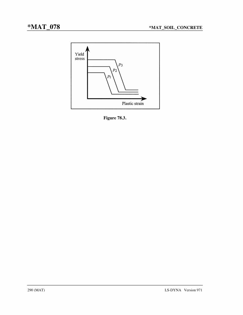
*MAT_078 *MAT_SOIL_CONCRETE
290 (MAT) LS-DYNA Version 971
Figure 78.3.
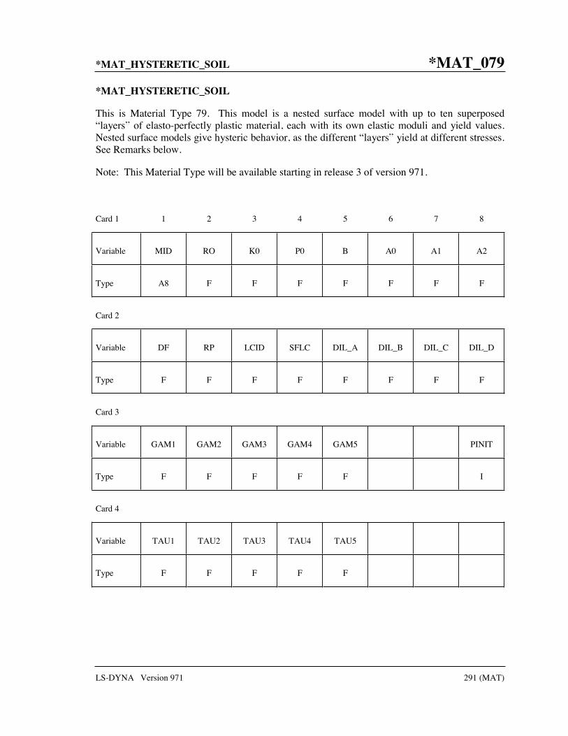
*MAT_HYSTERETIC_SOIL *MAT_079
LS-DYNA Version 971 291 (MAT)
*MAT_HYSTERETIC_SOIL
This is Material Type 79. This model is a nested surface model with up to ten superposed “layers” of elasto-perfectly plastic material, each with its own elastic moduli and yield values. Nested surface models give hysteric behavior, as the different “layers” yield at different stresses. See Remarks below.
Note: This Material Type will be available starting in release 3 of version 971.
Card 1 1 2 3 4 5 6 7 8
Variable MID RO K0 P0 B A0 A1 A2
Type A8 F F F F F F F
Card 2
Variable DF RP LCID SFLC DIL_A DIL_B DIL_C DIL_D
Type F F F F F F F F
Card 3
Variable GAM1 GAM2 GAM3 GAM4 GAM5 PINIT
Type F F F F F I
Card 4
Variable TAU1 TAU2 TAU3 TAU4 TAU5
Type F F F F F

*MAT_079 *MAT_HYSTERETIC_SOIL
292 (MAT) LS-DYNA Version 971
VARIABLE DESCRIPTION
MID Material identification. A unique number or label not exceeding 8 characters must be specified.
RO Mass density
K0 Bulk modulus at the reference pressure
P0 Cut-off/datum pressure (must be 0 i.e. tensile). Below this pressure, stiffness and strength disappears; this is also the “zero” pressure for pressure-varying properties.
B Exponent for pressure-sensitive moduli, b: ( )( )
0
0
b
o
b
o
G G p p
K K p p
= −
= −. b, must lie
in the range 0 b<1. Values close to 1 are not recommended because the pressure becomes indeterminate.
A0 Yield function constant a0 (Default = 1.0), see Material Type 5.
A1 Yield function constant a1 (Default = 0.0), see Material Type 5.
A2 Yield function constant a2 (Default = 0.0), see Material Type 5.
DF Damping factor. Must be in the range 0 df 1: EQ.0: no damping, EQ.1: maximum damping.
RP Reference pressure for following input data.
LCID Load curve ID defining shear strain verses shear stress. Up to ten points may be defined in the load curve. See *DEFINE_CURVE.
SFLD Scale factor to apply to shear stress in LCID.
DIL_A Dilation parameter A
DIL_B Dilation parameter B
DIL_C Dilation parameter C
DIL_D Dilation parameter D
GAM1 γ1, shear strain (ignored if LCID is non zero).
GAM2 γ2, shear strain (ignored if LCID is non zero).

*MAT_HYSTERETIC_SOIL *MAT_079
LS-DYNA Version 971 293 (MAT)
VARIABLE DESCRIPTION
GAM3 γ3, shear strain (ignored if LCID is non zero).
GAM4 γ4, shear strain (ignored if LCID is non zero).
GAM5 γ5, shear strain (ignored if LCID is non zero).
TAU1 τ1, shear stress at γ1 (ignored if LCID is non zero).
TAU2 τ2, shear stress at γ2 (ignored if LCID is non zero).
TAU3 τ3, shear stress at γ3 (ignored if LCID is non zero).
TAU4 τ4, shear stress at γ4 (ignored if LCID is non zero).
TAU5 τ5, shear stress at γ5 (ignored if LCID is non zero).
PINIT Flag for pressure sensitivity (B and A0, A1, A2 equations): EQ.0: Use current pressure (will vary during the analysis) EQ.1: Use pressure from initial stress state EQ.2: Use initial “plane stress” pressure ( ) / 2σ σ+v h
EQ.3: Use (compressive) initial vertical stress
Remarks:
The elastic moduli G and K are pressure sensitive:
( ) ( )( )
( ) ( )( )
0 0
0
0 0
0
b
b
ref
b
b
ref
G p pG p
p p
K p pK p
p p
−=
−
−=
−
where G0 and K0 are the input values, p is the current pressure, p0 the cut-off or datum pressure (must be zero or negative). If p attempts to fall below p0 (i.e., more tensile) the shear stresses are set to zero and the pressure is set to p0. Thus, the material has no stiffness or strength in tension. The pressure in compression is calculated as follows:
( ) ( )1
10 ln bp K V −= −
where V is the relative volume, i.e., the ratio between the original and current volume.

*MAT_079 *MAT_HYSTERETIC_SOIL
294 (MAT) LS-DYNA Version 971
The constants a0, a1, a2 govern the pressure sensitivity of the yield stress. Only the ratios between these values are important - the absolute stress values are taken from the stress-strain curve.
The stress strain pairs define a shear stress versus shear strain curve. The first point on the curve is assumed by default to be (0,0) and does not need to be entered. The slope of the curve must decrease with increasing γ. This curves applies at the reference pressure; at other pressures the curve is scaled by
( )( )
( ) ( )
( ) ( )
2
0 1 0 2 0
2
0 1 0 2 0
,
,ref ref ref
a a p p a p pp
p a a p p a p p
τ γτ γ
+ − + −=
+ − + −
The shear stress-strain curve (with points (τ1,γ1), (τ2,γ2)...(τN,γN)) is converted into a series of N
elastic perfectly-plastic curves such that ( )( ) ( ),iτ γ τ γ= , as shown in the figure below.
Figure 79.1
Each elastic perfectly-plastic curve represents one “layer” in the material model. Deviatoric stresses are stored and calculated separately for each layer. The yield surface for each layer is defined in terms of stress invariant J2; this is converted internally from the input values of maximum shear stress, assuming a uniaxial stress state:
( )2
max2
4:
2 3ii
i iJτσσ ′′= <

*MAT_HYSTERETIC_SOIL *MAT_079
LS-DYNA Version 971 295 (MAT)
where subscript i denotes layer i and τmaxi is the plastic shear stress of the layer.
In cases where the deviatoric stress state is closer to pure shear, the maximum shear stress
reached by the material will be up to 43 times higher than the input curve. Users may wish to
allow for this by reducing the input curve by this factor. When performing checks on the output, the following relationships may be useful:
Input shear stress is treated by the material model as 0.5* 3 :8
iiVon Mises Stress
σσ ′′=
Input shear strain is treated by the material model as 1.5* 3 :2
iiVon Mises Strain
εε ′′=
The total deviatoric stress is the sum of the deviatoric stresses in each layer. By this method, hysteretic (energy-absorbing) stress-strain curves are generated in response to any strain cycle of amplitude greater than the lowest yield strain of any layer. The example below shows response to small and large strain cycles (blue and pink lines) superposed on the input curve (thick red line).
Figure 79.2
Pressure Sensitivity The yield stresses of the layers, and hence the stress at each point on the shear stress-strain input curve, vary with pressure according to constants A0, A1 and A2. The elastic moduli, and hence also the slope of each section of shear stress-strain curve, vary with pressure according to constant B. These effects combine to modify the shear stress-strain curve according to pressure:

*MAT_079 *MAT_HYSTERETIC_SOIL
296 (MAT) LS-DYNA Version 971
Figure 79.3
Pressure sensitivity can make the solution sensitive to numerical noise. In cases where the expected pressure changes are small compared to the initial stress state, it may be preferable to use pressure from the initial stress state instead of current pressure as the basis for the pressure sensitivity (option PINIT). This causes the bulk modulus and shear stress-strain curve to be calculated once for each element at the start of the analysis and to remain fixed thereafter. PINIT affects both stiffness (calculated using B) and strength (calculated using A0, A1 and A2). If PINIT options 2 (“plane stress” pressure) or 3 (vertical stress) are used, these quantities substitute for pressure p in the equations above. Input values of pref and p0 should then also be “plane stress” pressure or vertical stress, respectively.
If PINIT is used, B is allowed to be as high as 1.0 (stiffness proportional to initial pressure); otherwise, values of B higher than about 0.5 are not recommended.
Dilatancy Parameters DIL_A, DIL_B, DIL_C and DIL_D control the compaction and dilatancy that occur in sandy soils as a result of shearing motion. The dilatancy is expressed as a volume strain γv:
v r g
_r
g
12 2 2
12 2 2
_ ( )
*
_ _ * *
( )
* ( )
, 2 ,2
DIL B
xz yz
xz yz
xz yz xz yz
DIL A
G
DIL C DIL D G
G d d
ε ε ε
ε
ε
γ γ
γ γ
γ γ ε ε
= +
= Γ
=+
Γ = +
= +
=
Stress varies with pressure according to A0, A1, A2 Slope varies
with pressure according to B
At different pressures, the same point on the input stress-strain curve will be reached at different strain values.
Shear stress-strain response at pressure P1
Shear stress-strain response at pressure P2

*MAT_HYSTERETIC_SOIL *MAT_079
LS-DYNA Version 971 297 (MAT)
γr describes the dilation of the soil due to the magnitude of the shear strains; this is caused by the soil particles having to climb over each other to develop shear strain.
γg describes compaction of the soil due to collapse of weak areas and voids, caused by continuous shear straining.
Recommended inputs for sandy soil:
DIL_A 10 DIL_B 1.6 DIL_C -100 DIL_D -2.5
DIL_A and DIL_B may cause instabilites in some models. If this facility is used with pore water pressure, liquefaction can be modeled.

*MAT_080 *MAT_RAMBERG-OSGOOD
298 (MAT) LS-DYNA Version 971
*MAT_RAMBERG-OSGOOD
This is Material Type 80. This model is intended as a simple model of shear behavior and can be used in seismic analysis.
Card 1 1 2 3 4 5 6 7 8
Variable MID RO GAMY TAUY ALPHA R BULK
Type A8 F F F F F F
Default none none none none none none none
VARIABLE DESCRIPTION
MID Material identification. A unique number or label not exceeding 8 characters must be specified.
RO Mass density.
GAMY Reference shear strain (γy)
TAUY Reference shear stress (τy)
ALPHA Stress coefficient (α)
R Stress exponent (r)
BULK Elastic bulk modulus
Remarks:
The Ramberg-Osgood equation is an empirical constitutive relation to represent the one-dimensional elastic-plastic behavior of many materials, including soils. This model allows a simple rate independent representation of the hysteretic energy dissipation observed in soils subjected to cyclic shear deformation. For monotonic loading, the stress-strain relationship is given by:
0
0
r
y y y
r
y y y
if
if
γ τ τα γγ τ τ
γ τ τα γγ τ τ
= + ≥
= − <

*MAT_RAMBERG-OSGOOD *MAT_080
LS-DYNA Version 971 299 (MAT)
where γ is the shear and τ is the stress. The model approaches perfect plasticity as the stress exponent r → ∞ . These equations must be augmented to correctly model unloading and reloading material behavior. The first load reversal is detected by 0γγ < . After the first reversal, the stress-strain relationship is modified to
( ) ( ) ( )
( ) ( ) ( )
0 0 0
0 0 0
02 2 2
02 2 2
y y y
y y y
if
if
γ γ τ τ τ τα γ
γ τ τ
γ γ τ τ τ τα γ
γ τ τ
′− − −= + ≥
′− − −= − <
where 0γ and 0τ represent the values of strain and stress at the point of load reversal.
Subsequent load reversals are detected by ( )0 0γ γ γ− < .
The Ramberg-Osgood equations are inherently one-dimensional and are assumed to apply to shear components. To generalize this theory to the multidimensional case, it is assumed that each component of the deviatoric stress and deviatoric tensorial strain is independently related by the one-dimensional stress-strain equations. A projection is used to map the result back into deviatoric stress space if required. The volumetric behavior is elastic, and, therefore, the pressure p is found by
vp Kε= −
where vε is the volumetric strain.

*MAT_081-082 *MAT_PLASTICITY_WITH_DAMAGE
300 (MAT) LS-DYNA Version 971
*MAT_PLASTICITY_WITH_DAMAGE_{OPTION}
This is Material Types 81 and 82. An elasto-visco-plastic material with an arbitrary stress versus strain curve and arbitrary strain rate dependency can be defined. Damage is considered before rupture occurs. Also, failure based on a plastic strain or a minimum time step size can be defined.
Available options include:
<BLANK>
ORTHO
ORTHO_RCDC
Including ORTHO invokes an orthotropic damage model. It is implemented only for shell elements with multiple through thickness integration points and is an extension to include orthotropic damage as a means of treating failure in aluminum panels. Directional damage begins after a defined failure strain is reached in tension and continues to evolve until a tensile rupture strain is reached in either one of the two orthogonal directions. After rupture is detected at all integration points, the element is deleted. The option ORTHO_RCDC invokes the damage model developed by Wilkins [Wilkins, et al. 1977]. A nonlocal formulation, which requires additional storage, is used if a characteristic length is defined. The RCDC option, which was added at the request of Toyota, works well in predicting failure in cast aluminum see Yamasaki, et al., [2006].
Card 1 1 2 3 4 5 6 7 8
Variable MID RO E PR SIGY ETAN EPPF TDEL
Type A8 F F F F F F F
Default none none none none none 0.0 10.E+20 10.E+20
Card 2
Variable C P LCSS LCSR EPPFR VP LCDM NUMINT
Type F F F F F F F I
Default 0 0 0 0 0 0 0 0

*MAT_PLASTICITY_WITH_DAMAGE *MAT_081-082
LS-DYNA Version 971 301 (MAT)
Card 3 1 2 3 4 5 6 7 8
Variable EPS1 EPS2 EPS3 EPS4 EPS5 EPS6 EPS7 EPS8
Type F F F F F F F F
Default 0 0 0 0 0 0 0 0
Card 4
Variable ES1 ES2 ES3 ES4 ES5 ES6 ES7 ES8
Type F F F F F F F F
Default 0 0 0 0 0 0 0 0
Read the following card if the option ORTHO_RCDC is active.
Card 5 1 2 3 4 5 6 7 8
Variable ALPHA BETA GAMMA D0 B LAMBDA DS L
Type F F F F F F F F
Default 0 0 0 0 0 0 0 0
VARIABLE DESCRIPTION
MID Material identification. A unique number or label not exceeding 8 characters must be specified.
RO Mass density.
E Young’s modulus.
PR Poisson’s ratio.
SIGY Yield stress.

*MAT_081-082 *MAT_PLASTICITY_WITH_DAMAGE
302 (MAT) LS-DYNA Version 971
VARIABLE DESCRIPTION
ETAN Tangent modulus, ignored if (LCSS.GT.0) is defined.
EPPF Plastic strain, fs, at which material softening begins (logarithmic).
TDEL Minimum time step size for automatic element deletion.
C Strain rate parameter, C, see formula below.
P Strain rate parameter, P, see formula below.
LCSS Load curve ID or Table ID. Load curve ID defining effective stress versus effective plastic strain. If defined EPS1-EPS8 and ES1-ES8 are ignored. The table ID defines for each strain rate value a load curve ID giving the stress versus effectiveplastic strain for that rate, See Figure 24.1. The stress versus effective plastic strain curve for the lowest value of strain rate is used if the strain rate falls below the minimum value. Likewise, the stress versus effective plastic strain curve for the highest value of strain rate is used if the strain rate exceeds the maximum value. The strain rate parameters: C and P;
LCSR Load curve ID defining strain rate scaling effect on yield stress.
EPPFR Plastic strain at which material ruptures (logarithmic).
VP Formulation for rate effects: EQ.0.0: Scale yield stress (default), EQ.1.0: Viscoplastic formulation.
LCDM Load curve ID defining nonlinear damage curve.
NUMINT Number of through thickness integration points which must fail before the element is deleted. (If zero, all points must fail.) The default of all integration points is not recommended since elements undergoing large strain are often not deleted due to nodal fiber rotations which limit strains at active integration points after most points have failed. Better results are obtained if NUMINT is set to 1 or a number less than one half of the number of through thickness points. For example, if four through thickness points are used, NUMINT should not exceed 2, even for fully integrated shells which have 16 integration points.
EPS1-EPS8 Effective plastic strain values (optional if SIGY is defined). At least 2 points should be defined.
ES1-ES8 Corresponding yield stress values to EPS1 - EPS8.
ALPHA Parameter α . for the Rc-Dc model

*MAT_PLASTICITY_WITH_DAMAGE *MAT_081-082
LS-DYNA Version 971 303 (MAT)
VARIABLE DESCRIPTION
BETA Parameter β . for the Rc-Dc model
GAMMA Parameter γ . for the Rc-Dc model
D0 Parameter 0D . for the Rc-Dc model
B Parameter b . for the Rc-Dc model
LAMBDA Parameter λ . for the Rc-Dc model
DS Parameter sD . for the Rc-Dc model
L Optional characteristic element length for this material. We recommend that the default of 0 always be used, especially in parallel runs. If zero, nodal values of the damage function are used to compute the damage gradient. See discussion below.
Remarks:
The stress strain behavior may be treated by a bilinear stress strain curve by defining the tangent modulus, ETAN. Alternately, a curve similar to that shown in Figure 10.1 is expected to be defined by (EPS1,ES1) - (EPS8,ES8); however, an effective stress versus effective plastic strain curve (LCSS) may be input instead if eight points are insufficient. The cost is roughly the same for either approach. The most general approach is to use the table definition (LCSS) discussed below.
Two options to account for strain rate effects are possible:
I. Strain rate may be accounted for using the Cowper and Symonds model which scales the yield stress with the factor
16
1C
ε+
where ε is the strain rate, ij ijε ε ε= .
If the viscoplastic option is active, VP=1.0, and if SIGY is > 0 then the dynamic yield
stress is computed from the sum of the static stress, ( )s py effσ ε , which is typically given by a load
curve ID, and the initial yield stress, SIGY, multiplied by the Cowper-Symonds rate term as follows:

*MAT_081-082 *MAT_PLASTICITY_WITH_DAMAGE
304 (MAT) LS-DYNA Version 971
( ) ( )1
,p peffp p s p
y eff eff y eff SIGYC
εσ ε ε σ ε= + ⋅
where the plastic strain rate is used. With this latter approach similar results can be obtained between this model and material model: *MAT_ANISOTROPIC_VISCOPLASTIC. If SIGY=0,
the following equation is used instead where the static stress, ( )s py effσ ε , must be defined by a
load curve:
( ) ( )1
, 1p p
effp p s py eff eff y eff C
εσ ε ε σ ε= +
This latter equation is always used if the viscoplastic option is off.
II. For complete generality a load curve (LCSR) to scale the yield stress may be input instead. In this curve the scale factor versus strain rate is defined.
The constitutive properties for the damaged material are obtained from the undamaged material properties. The amount of damage evolved is represented by the constant, ω , which varies from zero if no damage has occurred to unity for complete rupture. For uniaxial loading, the nominal stress in the damaged material is given by
nominal
P
Aσ =
where P is the applied load and A is the surface area. The true stress is given by:
trueloss
P
A Aσ =
−
where lossA is the void area. The damage variable can then be defined:
lossA
Aω = 0 1ω≤ ≤
In this model damage is defined in terms of plastic strain after the failure strain is exceeded:
p p
eff failure p p pfailure eff rupturep p
rupture failure
ifε ε
ω ε ε εε ε
−= ≤ ≤
−
After exceeding the failure strain softening begins and continues until the rupture strain is reached.
The Rc-Dc model is defined as the following:

*MAT_PLASTICITY_WITH_DAMAGE *MAT_081-082
LS-DYNA Version 971 305 (MAT)
The damage D is given by
1 2pD dω ω ε=
where pε is the equivalent plastic strain,
1
1
1 m
α
ωγσ
=−
is a triaxial stress weighting term and
( )2 2 DAβω = −
is a asymmetric strain weighting term. In the above mσ is the mean stress and
2 3
3 2
min ,D
S SA
S S=
Fracture is initiated when the accumulation of damage is
1c
D
D>
where cD is the a critical damage given by
( )0 1cD D b Dλ= + ∇
A fracture fraction,
c
s
D DF
D
−=
defines the degradations of the material by the Rc-Dc model.
For the Rc-Dc model the gradient of damage needs to be estimated. The damage is connected to the integration points, and, thus, the computation of the gradient requires some manipulation of the LS-DYNA source code. Provided that the damage is connected to nodes, it can be seen as a standard bilinear field and the gradient is easily obtained. To enable this, the damage at the integration points are transferred to the nodes as follows. Let nE be the set of
elements sharing node n , nE the number of elements in that set, eP the set of integration points
in element e and eP the number of points in that set. The average damage eD in element e is
computed as
e
Ppp
e P
D
D e∈=

*MAT_081-082 *MAT_PLASTICITY_WITH_DAMAGE
306 (MAT) LS-DYNA Version 971
where pD is the damage in integration point p . Finally, the damage value in node n is
estimated as
n
ee E
nn
D
DE
∈= .
This computation is performed in each time step and requires additional storage. Currently we use three times the total number of nodes in the model for this calculation, but this could be reduced by a considerable factor if necessary. There is an Rc-Dc option for the Gurson dilatational-plastic model. In the implementation of this model, the norm of the gradient is computed differently. Let l
fE be the set of elements from within a distance l of element, f not
including the element itself, and let lfE be the number of elements in that set. The norm of the
gradient of damage is estimated roughly as
1lf
e f
lfe E eff
D DD
dE ∈
−∇ ≈
where efd is the distance between element f and e.
The reason for taking the first approach is that it should be a better approximation of the gradient, it can for one integration point in each element be seen as a weak gradient of an elementwise constant field. The memory consumption as well as computational work should not be much higher than for the other approach.
Figure 81-82.1. Stress strain behavior when damage is included.

*MAT_PLASTICITY_WITH_DAMAGE *MAT_081-082
LS-DYNA Version 971 307 (MAT)
Figure 81-82.2. A nonlinear damage curve is optional. Note that the origin of the curve is at (0,0). It is permissible to input the failure strain, fs, as zero for this option. The nonlinear damage curve is useful for controlling the softening behavior after the failure strain is reached.

*MAT_083 *MAT_FU_CHANG_FOAM
308 (MAT) LS-DYNA Version 971
*MAT_FU_CHANG_FOAM
This is Material Type 83. Rate effects can be modeled in low and medium density foams, see Figure 83.1. Hysteretic unloading behavior in this model is a function of the rate sensitivity with the most rate sensitive foams providing the largest hysteresis and vice versa. The unified constitutive equations for foam materials by Chang [1995] provides the basis for this model. The mathematical description given below is excerpted from the reference. Further improvements have been incorporated based on work by Hirth, Du Bois, and Weimar [1998]. Their improvements permit: load curves generated by drop tower test to be directly input, a choice of principal or volumetric strain rates, load curves to be defined in tension, and the volumetric behavior to be specified by a load curve. The unloading response was generalized by Kolling, Hirth, Erhart and Du Bois [2006].
Card 1 1 2 3 4 5 6 7 8
Variable MID RO E ED TC FAIL DAMP TBID
Type A8 F F F F F F F
Default --- --- --- --- 1.E+20
Remarks --- --- --- --- --- 5
Card 2
Variable BVFLAG SFLAG RFLAG TFLAG PVID SRAF REF HU
Type F F F F F F F F
Default 1.0 0.0 0.0 0.0 0.0 0.0 0.0 1.0
Remarks 1 2 3 4 5

*MAT_FU_CHANG_FOAM *MAT_083
LS-DYNA Version 971 309 (MAT)
Card 3 1 2 3 4 5 6 7 8
Variable D0 N0 N1 N2 N3 C0 C1 C2
Type F F F F F F F F
Default 0.0 0.0 0.0 0.0 0.0 0.0 0.0 0.0
Card 4
Variable C3 C4 C5 AIJ SIJ MINR MAXR SHAPE
Type F F F F F F F F
Default 0.0 0.0 0.0 0.0 0.0 0.0 0.0 0.0
VARIABLE DESCRIPTION
MID Material identification. A unique number or label not exceeding 8 characters must be specified.
RO Mass density
E Young’s modulus
ED Optional Young's relaxation modulus, dE , for rate effects. See
comments below. EQ.0.0: Maximum slope in stress vs. strain curve is used. When
the maximum slope is taken for the contact, the time step size for this material is reduced for stability. In some cases Δt may be significantly smaller, and defining a reasonable stiffness is recommended.
TC Tension cut-off stress
FAIL Failure option after cutoff stress is reached: EQ.0.0: tensile stress remains at cut-off value, EQ.1.0: tensile stress is reset to zero.
DAMP Viscous coefficient (.05< recommended value <.50) to model damping effects.

*MAT_083 *MAT_FU_CHANG_FOAM
310 (MAT) LS-DYNA Version 971
VARIABLE DESCRIPTION
TBID Table ID, see *DEFINE_TABLE, for nominal stress vs. strain data as a function of strain rate. If the table ID is provided, cards 3 and 4 may be left blank and the fit will be done internally. The Table ID can be positive or negative (see remark 5 below).
BVFLAG Bulk viscosity activation flag, see remark below: EQ.0.0: no bulk viscosity (recommended), EQ.1.0: bulk viscosity active.
SFLAG Strain rate flag (see remark 2 below): EQ.0.0: true constant strain rate, EQ.1.0: engineering strain rate.
RFLAG Strain rate evaluation flag: EQ.0.0: first principal direction, EQ.1.0: principal strain rates for each principal direction, EQ.2.0: volumetric strain rate.
TFLAG Tensile stress evaluation: EQ.0.0: linear in tension. EQ.1.0: input via load curves with the tensile response corresponds
to negative values of stress and strain.
PVID Optional load curve ID defining pressure versus volumetric strain.
SRAF Strain rate averaging flag. EQ.0.0: use weighted running average.
EQ.1.0: average the last twelve values.
REF Use reference geometry to initialize the stress tensor. The reference geometry is defined by the keyword: *INITIAL_FOAM_REFERENCE _GEOMETRY (see there for more details).
EQ.0.0: off, EQ.1.0: on.
HU Hysteretic unloading factor between 0 and 1 (default=1, i.e., no energy dissipation), see also Figure 22.57.1.
D0 material constant, see equations below.
N0 material constant, see equations below.
N1 material constant, see equations below.
N2 material constant, see equations below.
N3 material constant, see equations below.

*MAT_FU_CHANG_FOAM *MAT_083
LS-DYNA Version 971 311 (MAT)
VARIABLE DESCRIPTION
C0 material constant, see equations below.
C1 material constant, see equations below.
C2 material constant, see equations below.
C3 material constant, see equations below.
C4 material constant, see equations below.
C5 material constant, see equations below.
AIJ, material constant, see equations below.
SIJ material constant, see equations below.
MINR Ratemin, minimum strain rate of interest.
MAXR Ratemax, maximum strain rate of interest.
SHAPE Shape factor for unloading. Active for nonzero values of the hysteretic unloading factor HU. Values less than one reduces the energy dissipation and greater than one increases dissipation, see also Figure 57.1.
Remarks:
The strain is divided into two parts: a linear part and a non-linear part of the strain
( ) ( ) ( )L NE t E t E t= +
and the strain rate become
( ) ( ) ( )L NE t E t E t= +
NE is an expression for the past history of NE . A postulated constitutive equation may be written as:
( ) ( ) ( )0
,Ntt E S t d
τ
σ τ τ∞
=
=
where ( )S t is the state variable and . 0τ
∞
=
is a functional of all values of τ in : 0Tτ τ≤ ≤ ∞ and
( ) ( )N NtE E tτ τ= −

*MAT_083 *MAT_FU_CHANG_FOAM
312 (MAT) LS-DYNA Version 971
where τ is the history parameter:
( )NtE the virgin materialτ = ∞ ⇔
It is assumed that the material remembers only its immediate past, i.e., a neighborhood about 0τ = . Therefore, an expansion of ( )N
tE τ in a Taylor series about 0τ = yields:
( ) ( ) ( )0 0N
N N tt
EE E dt
tτ ∂= +
∂
Hence, the postulated constitutive equation becomes:
( ) ( ) ( ) ( )( ), ,N Nt E t E t S tσ σ ∗=
where we have replaced NtE
t
∂∂
by NE , and σ ∗ is a function of its arguments.
For a special case,
( ) ( ) ( )( ),Nt E t S tσ σ ∗=
we may write
( ) ( )( ),NtE f S t s t=
which states that the nonlinear strain rate is the function of stress and a state variable which represents the history of loading. Therefore, the proposed kinetic equation for foam materials is:
( )( )
02
0 0 2exp
n
Nt
tr SE D c
σσσ σ
= −
where D0, c0, and n0 are material constants, and S is the overall state variable. If either 0 0D = or
0c → ∞ then the nonlinear strain rate vanishes.
( ) ( ) 21
1 2 3
nn N
ij ij ij ijS c a R c S P c W E I R= − +
3
45
1 1
nNE
R cc
= + −
( )( )( )
NP tr E
W tr dE
σ
σ
=
=

*MAT_FU_CHANG_FOAM *MAT_083
LS-DYNA Version 971 313 (MAT)
where c1, c2, c3, c4, c5, n1, n2, n3, and aij are material constants and:
( )( )
( )
12
12
1
2
ij ij
ij ij
N N Nij ij
E E E
E E E
σ σ σ=
=
=
In the implementation by Fu Chang the model was simplified such that the input constants ija
and the state variables ijS are scalars.
Figure 83.1. Nominal stress versus engineering strain curves, which are used to model rate effects in Fu Chang’s foam model.
Optional Tensile Curves (TFLAG=1)
Compressive
3ε
3 2 1ε ε ε> >
Default Tensile Behavior(TFLAG=0)
2ε
1ε

*MAT_083 *MAT_FU_CHANG_FOAM
314 (MAT) LS-DYNA Version 971
Additional Remarks:
1. The bulk viscosity, which generates a rate dependent pressure, may cause an unexpected volumetric response and consequently, it is optional with this model.
2. Dynamic compression tests at the strain rates of interest in vehicle crash are usually performed with a drop tower. In this test the loading velocity is nearly constant but the true strain rate, which depends on the instantaneous specimen thickness, is not. Therefore, the engineering strain rate input is optional so that the stress strain curves obtained at constant velocity loading can be used directly.
3. To further improve the response under multiaxial loading, the strain rate parameter can either be based on the principal strain rates or the volumetric strain rate.
4. Correlation under triaxial loading is achieved by directly inputting the results of hydrostatic testing in addition to the uniaxial data. Without this additional information which is fully optional, triaxial response tends to be underestimated.
5. Several options are available to control unloading response in MAT_083:
1) HU=0 and TBID>0
This is the old way. In this case the unloading response will follow the curve with the lowest strain rate and is rate-independent. The curve with lowest strain rate value (typically zero) in TBID should correspond to the unloading path of the material as measured in a quasistatic test. The quasistatic loading path then corresponds to a realistic (small) value of the strain rate.
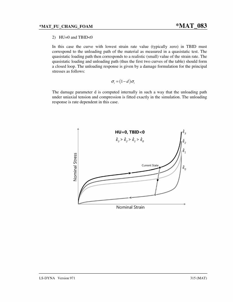
*MAT_FU_CHANG_FOAM *MAT_083
LS-DYNA Version 971 315 (MAT)
2) HU=0 and TBID<0
In this case the curve with lowest strain rate value (typically zero) in TBID must correspond to the unloading path of the material as measured in a quasistatic test. The quasistatic loading path then corresponds to a realistic (small) value of the strain rate. The quasistatic loading and unloading path (thus the first two curves of the table) should form a closed loop. The unloading response is given by a damage formulation for the principal stresses as follows:
( )1i idσ σ= −
The damage parameter d is computed internally in such a way that the unloading path under uniaxial tension and compression is fitted exactly in the simulation. The unloading response is rate dependent in this case.

*MAT_083 *MAT_FU_CHANG_FOAM
316 (MAT) LS-DYNA Version 971
3) HU>0 and TBID>0
No unloading curve should be provided in the table and the curve with the lowest strain rate value in TBID should correspond to the loading path of the material as measured in a quasistatic test. In this case the unloading response is given by a damage formulation for the principal stresses as follows:
( )
( )max
1
1 1
i i
SHAPE
cur
d
Wd HU
W
σ σ= −
= − − ,
where W corresponds to the current value of the hyperelastic energy per unit undeformed volume. The unloading response is rate dependent in this case.

*MAT_WINFRITH_CONCRETE *MAT_084-085
LS-DYNA Version 971 317 (MAT)
*MAT_WINFRITH_CONCRETE
This is Material Type 84 and Material Type 85, only the former of which includes rate effects. The Winfrith concrete model is a smeared crack (sometimes known as pseudo crack), smeared rebar model, implemented in the 8-node single integration point continuum element. This model was developed by Broadhouse and Neilson [1987], and Broadhouse [1995] over many years and has been validated against experiments. The input documentation given here is taken directly form the report by Broadhouse. The Fortran subroutines and quality assurance test problems were also provided to LSTC by the Winfrith Technology Center. The rebar is defined in the section: *MAT_WINFRITH_CONCRETE_REINFORCEMENT which follows.
Card 1 1 2 3 4 5 6 7 8
Variable MID RO TM PR UCS UTS FE ASIZE
Type A8 F F F F F F F
Card 2
Variable E YS EH UELONG RATE CONM CONL CONT
Type F F F F F F F F
Card 3
Variable EPS1 EPS2 EPS3 EPS4 EPS5 EPS6 EPS7 EPS8
Type F F F F F F F F
Card 4
Variable P1 P2 P3 P4 P5 P6 P7 P8
Type F F F F F F F F

*MAT_084-085 *MAT_WINFRITH_CONCRETE
318 (MAT) LS-DYNA Version 971
VARIABLE DESCRIPTION
MID Material identification. A unique number or label not exceeding 8 characters must be specified.
RO Mass density.
TM Initial tangent modulus of concrete.
PR Poisson's ratio.
UCS Uniaxial compressive strength.
UTS Uniaxial tensile strength.
FE Depends on value of RATE below. RATE.EQ.0: Fracture energy (energy per unit area dissipated in
opening crack). RATE.EQ.1: Crack width at which crack-normal tensile stress goes to
zero.
ASIZE Aggregate size (radius).
E Young's modulus of rebar.
YS Yield stress of rebar.
EH Hardening modulus of rebar
UELONG Ultimate elongation before rebar fails.
RATE Rate effects: EQ.0.0: strain rate effects are included (mat 84 - recommended). EQ.1.0: strain rate effects are turned off (mat 85).
CONM GT.0: Factor to convert model mass units to kg.
EQ.-1.: Mass, length, time units in model are lbf*sec2/in, inch, sec. EQ -2.: Mass, length, time units in model are g, cm, microsec. EQ.-3.: Mass, length, time units in model are g, mm, msec. EQ.-4.: Mass, length, time units in model are metric ton, mm, sec. EQ.-5.: Mass, length, time units in model are kg, mm, msec.
CONL If CONM.GT.0, factor to convert model length units to meters; otherwise CONL is ignored.
CONT If CONM.GT.0, factor to convert model time units to seconds; otherwise CONT is ignored.

*MAT_WINFRITH_CONCRETE *MAT_084-085
LS-DYNA Version 971 319 (MAT)
VARIABLE DESCRIPTION
EPS1,..... Volumetric strain values (natural logarithmic values), see comments below. A maximum of 8 values are allowed. The tabulated values mustcompletely cover the expected values in the analysis. If the first value is not for a volumetric strain value of zero then the point (0.0,0.0) will be automatically generated and up to a further nine additional values may be defined.
P1, P2,..PN Pressures corresponding to volumetric strain values.
Remarks:
Pressure is positive in compression; volumetric strain is given by the natural log of the relative volume and is negative in compression. The tabulated data are given in order of increasing compression, with no initial zero point.
If the volume compaction curve is omitted, the following scaled curve is automatically used where 1p is the pressure at uniaxial compressive failure from:
1 3cp
σ=
and K is the bulk unloading modulus computed from
( )3 1 2sE
Kv
=−
where sE is the input tangent modulus for concrete and v is Poisson's ratio.

*MAT_084-085 *MAT_WINFRITH_CONCRETE
320 (MAT) LS-DYNA Version 971
Volumetric Strain Pressure (MPa)
-p1/K 1.00xp1
-0.002 1.50xp1
-0.004 3.00xp1
-0.010 4.80xp1
-0.020 6.00xp1
-0.030 7.50xp1
-0.041 9.45xp1
-0.051 11.55xp1
-0.062 14.25xp1
-0.094 25.05xp1
Table 84-85.1 Default pressure versus volumetric strain curve for concrete if the curve is not defined.
The Winfrith concrete model generates an additional binary output database containing information on crack locations, directions, and widths. In order to generate the crack database, the LS-DYNA execution line is modified by adding:
q=crf where crf is the name of the crack database (e.g., q=DYNCRCK).
LS-Prepost can display the cracks on the deformed mesh plots. To do so, read the d3plot database into LS-Prepost and then select File > Open > Crack from the top menu bar. Or, open the crack database by adding the following to the LS-Prepost execution line:
q=crf where crf is the name of the crack database (e.g., q=DYNCRCK).
By default, all the cracks in visible elements are shown. You can eliminate narrow cracks from the display by setting a minimum crack width for displayed cracks. Do this by choosing Setting > Concrete Crack Width. From the top menu bar of LS-Prepost, choosing Misc > Model Info will reveal the number of cracked elements and the maximum crack width in a given plot state.

*MAT_WINFRITH_CONCRETE_REINFORCEMENT *MAT_084
LS-DYNA Version 971 321 (MAT)
*MAT_WINFRITH_CONCRETE_REINFORCEMENT
This is Material Type 84 rebar reinforcement. Reinforcement may be defined in specific groups of elements, but it is usually more convenient to define a two-dimensional mat in a specified layer of a specified material. Reinforcement quantity is defined as the ratio of the cross-sectional area of steel relative to the cross-sectional area of concrete in the element (or layer). These cards may follow either one of two formats below and may also be defined in any order.
Option 1 (Reinforcement quantities in element groups).
1 2 3 4 5 6 7 8
Variable EID1 EID2 INC XR YR ZR
Type I I I F F F
Option 2 (Two dimensional layers by part ID).
1 2 3 4 5 6 7 8
Variable PID AXIS COOR RQA RQB
Type blank I I F F F
VARIABLE DESCRIPTION
EID1 First element ID in group.
EID2 Last element ID in group
INC Element increment for generation.
XR X-reinforcement quantity (for bars running parallel to global x-axis).
YR Y-reinforcement quantity (for bars running parallel to global y-axis).
ZR Z-reinforcement quantity (for bars running parallel to global z-axis).
PID Part ID of reinforced elements.
AXIS Axis normal to layer. EQ.1: A and B are parallel to global Y and Z, respectively. EQ.2: A and B are parallel to global X and Z, respectively. EQ.3: A and B are parallel to global X and Y, respectively.

*MAT_084 *MAT_WINFRITH_CONCRETE_REINFORCEMENT
322 (MAT) LS-DYNA Version 971
VARIABLE DESCRIPTION
COOR Coordinate location of layer (X-coordinate if AXIS.EQ.1; Y-coordinate if AXIS.EQ.2; Z-coordinate if AXIS.EQ.3.
RQA Reinforcement quantity (A).
RQB Reinforcement quantity (B).
Remarks:
1. Reinforcement quantity is the ratio of area of reinforcement in an element to the element's total cross-sectional area in a given direction. This definition is true for both Options 1 and 2. Where the options differ is in the manner in which it is decided which elements are reinforced. In Option 1, the reinforced element IDs are spelled out. In Option 2, elements of part ID PID which are cut by a plane (layer) defined by AXIS and COOR are reinforced.

*MAT_ORTHOTROPIC_VISCOELASTIC *MAT_086
LS-DYNA Version 971 323 (MAT)
*MAT_ORTHOTROPIC_VISCOELASTIC
This is Material Type 86. It allows the definition of an orthotropic material with a viscoelastic part. This model applies to shell elements.
Card 1 1 2 3 4 5 6 7 8
Variable MID RO EA EB EC VF K
Type A8 F F F F F F
Card 2
Variable G0 GINF BETA PRBA PRCA PRCB
Type F F F F F F
Card 3
Variable GAB GBC GCA AOPT MANGLE
Type F F F F F
Card 4
Variable A1 A2 A3
Type F F F
Card 5
Variable V1 V2 V3 D1 D2 D3
Type F F F F F F

*MAT_086 *MAT_ORTHOTROPIC_VISCOELASTIC
324 (MAT) LS-DYNA Version 971
VARIABLE DESCRIPTION
MID Material identification. A unique number or label not exceeding 8 characters must be specified.
RO Mass density
EA Young’s Modulus Ea
EB Young’s Modulus Eb
EC Young’s Modulus Ec
VF Volume fraction of viscoelastic material
K Elastic bulk modulus
G0 G0, short-time shear modulus
GINF G , long-time shear modulus
BETA β, decay constant
PRBA Poisson’s ratio, νba
PRCA Poisson’s ratio, νca
PRCB Poisson’s ratio, νcb
GAB Shear modulus, Gab
GBC Shear modulus, Gbc
GCA Shear modulus, Gca
AOPT Material axes option (see MAT_OPTION TROPIC_ELASTIC for a more complete description):
EQ.0.0: locally orthotropic with material axes determined by element nodes 1, 2, and 4, as with *DEFINE_COORDINATE_ NODES.
EQ.2.0: globally orthotropic with material axes determined by vectors defined below, as with *DEFINE_COORDINATE_ VECTOR.
EQ.3.0: locally orthotropic material axes determined by rotating the material axes about the element normal by an angle, MANGLE, from a line in the plane of the element defined by the cross product of the vector v with the element normal.

*MAT_ORTHOTROPIC_VISCOELASTIC *MAT_086
LS-DYNA Version 971 325 (MAT)
VARIABLE DESCRIPTION
LT.0.0: the absolute value of AOPT is a coordinate system ID number (CID on *DEFINE_COORDINATE_NODES, *DEFINE_ COORDINATE_SYSTEM or *DEFINE_COORDINATE_ VECTOR). Available in R3 version of 971 and later.
MANGLE Material angle in degrees for AOPT = 3, may be overridden on the element card, see *ELEMENT_SHELL_BETA.
A1 A2 A3 Define components of vector a for AOPT = 2.
V1 V2 V3 Define components of vector v for AOPT = 3.
D1 D2 D3 Define components of vector d for AOPT = 2.
Remarks:
For the orthotropic definition it is referred to Material Type 2 and 21.

*MAT_087 *MAT_CELLULAR_RUBBER
326 (MAT) LS-DYNA Version 971
*MAT_CELLULAR_RUBBER
This is Material Type 87. This material model provides a cellular rubber model with confined air pressure combined with linear viscoelasticity as outlined by Christensen [1980]. See Figure 87.1.
Card 1 1 2 3 4 5 6 7 8
Variable MID RO PR N
Type A8 F F I
Card 2 if N > 0, a least squares fit is computed from uniaxial data
Card 2 1 2 3 4 5 6 7 8
Variable SGL SW ST LCID
Type F F F F
Card 2 if N = 0, define the following constants
Card 2 1 2 3 4 5 6 7 8
Variable C10 C01 C11 C20 C02
Type F F F F F
Card 3
Variable P0 PHI IVS G BETA
Type F F F F F

*MAT_CELLULAR_RUBBER *MAT_087
LS-DYNA Version 971 327 (MAT)
VARIABLE DESCRIPTION
MID Material identification. A unique number or label not exceeding 8 characters must be specified.
RO Mass density
PR Poisson’s ratio, typical values are between .0 to .2. Due to the large compressibility of air, large values of Poisson’s ratio generates physically meaningless results.
N Order of fit (currently < 3). If n>0 then a least square fit is computed with uniaxial data. The parameters given on card 2 should be specified. Also see *MAT_MOONEY_RIVLIN_RUBBER (material model 27). A Poisson’s ratio of .5 is assumed for the void free rubber during the fit. The Poisson’s ratio defined on Card 1 is for the cellular rubber. A void fraction formulation is used.
Define, if N > 0:
SGL Specimen gauge length l0
SW Specimen width
ST Specimen thickness
LCID Load curve ID giving the force versus actual change ΔL in the gauge length.
Define, if N = 0:
C10 Coefficient, C10
C01 Coefficient, C01
C11 Coefficient, C11
C20 Coefficient, C20
C02 Coefficient, C02
P0 Initial air pressure, P0
PHI Ratio of cellular rubber to rubber density, Φ
IVS Initial volumetric strain, γ0
G Optional shear relaxation modulus, G , for rate effects (viscosity)
BETA Optional decay constant, 1β

*MAT_087 *MAT_CELLULAR_RUBBER
328 (MAT) LS-DYNA Version 971
Remarks:
Rubber is generally considered to be fully incompressible since the bulk modulus greatly exceeds the shear modulus in magnitude. To model the rubber as an unconstrained material a hydrostatic work term, ( )HW J , is included in the strain energy functional which is function of
the relative volume, J , [Ogden 1984]:
( ) ( ) ( ) ( )1 2 1 2, 0
13
1 1 3
23
2 2 3
, , 3 3n
p q
pq Hp q
W J J J C J J W J
J I I
J I I
=
−
−
= − − +
+
+
In order to prevent volumetric work from contributing to the hydrostatic work the first and second invariants are modified as shown. This procedure is described in more detail by Sussman and Bathe [1987].
The effects of confined air pressure in its overall response characteristics is included by augmenting the stress state within the element by the air pressure.
sk airij ij ijσ σ δ σ= −
where skijσ is the bulk skeletal stress and airσ is the air pressure computed from the equation:
0
1air p γσ
γ φ= −
+ −
where p0 is the initial foam pressure usually taken as the atmospheric pressure and γ defines the volumetric strain
01Vγ γ= − +
where V is the relative volume of the voids and γ0 is the initial volumetric strain which is typically zero. The rubber skeletal material is assumed to be incompressible.
Rate effects are taken into account through linear viscoelasticity by a convolution integral of the form:
( )0 ijkl
tkl
ij g t dεσ τ ττ
∂= −∂
or in terms of the second Piola-Kirchhoff stress, ijS , and Green's strain tensor, ijE ,
( )0 ijkl
tkl
ijS G t dετ ττ
∂= −∂

*MAT_CELLULAR_RUBBER *MAT_087
LS-DYNA Version 971 329 (MAT)
where ( )ijkl
g t τ− and ( )ijkl
G t τ− are the relaxation functions for the different stress measures.
This stress is added to the stress tensor determined from the strain energy functional.
Since we wish to include only simple rate effects, the relaxation function is represented by one term from the Prony series:
( ) 01
Nt
mm
g t e βα α −
=
= +
given by,
( ) 1tdg t E e β−=
This model is effectively a Maxwell fluid which consists of a damper and spring in series. We characterize this in the input by a shear modulus, G , and decay constant, 1β .
The Mooney-Rivlin rubber model (model 27) is obtained by specifying n=1 without air pressure and viscosity. In spite of the differences in formulations with Model 27, we find that the results obtained with this model are nearly identical with those of material type 27 as long as large values of Poisson’s ratio are used.
Figure 87.1. Cellular rubber with entrapped air. By setting the initial air pressure to zero, an open cell, cellular rubber can be simulated.

*MAT_088 *MAT_MTS
330 (MAT) LS-DYNA Version 971
*MAT_MTS
This is Material Type 88. The MTS model is due to Mauldin, Davidson, and Henninger [1990] and is available for applications involving large strains, high pressures and strain rates. As described in the foregoing reference, this model is based on dislocation mechanics and provides a better understanding of the plastic deformation process for ductile materials by using an internal state variable call the mechanical threshold stress. This kinematic quantity tracks the evolution of the material’s microstructure along some arbitrary strain, strain rate, and temperature-dependent path using a differential form that balances dislocation generation and recovery processes. Given a value for the mechanical threshold stress, the flow stress is determined using either a thermal-activation-controlled or a drag-controlled kinetics relationship. An equation-of-state is required for solid elements and a bulk modulus must be defined below for shell elements.
Card 1 1 2 3 4 5 6 7 8
Variable MID RO SIGA SIGI SIGS SIG0 BULK
Type A8 F F F F F F
Card 2
Variable HF0 HF1 HF2 SIGS0 EDOTS0 BURG CAPA BOLTZ
Type F F F F F F F F
Card 3
Variable SM0 SM1 SM2 EDOT0 GO PINV QINV EDOTI
Type F F F F F F F F

*MAT_MTS *MAT_088
LS-DYNA Version 971 331 (MAT)
Card 4 1 2 3 4 5 6 7 8
Variable G0I PINVI QINVI EDOTS G0S PINVS QINVS
Type F F F F F F F
Card 5
Variable RHOCPR TEMPRF ALPHA EPS0
Type F F
VARIABLE DESCRIPTION
MID Material identification. A unique number or label not exceeding 8 characters must be specified.
RO Mass density
SIGA ˆaσ , dislocation interactions with long-range barriers (force/area).
SIGI ˆiσ , dislocation interactions with interstitial atoms (force/area).
SIGS ˆsσ , dislocation interactions with solute atoms (force/area).
SIG0 0σ , initial value of σ at zero plastic strain (force/area) NOT USED.
HF0 0a , dislocation generation material constant (force/area).
HF1 1a , dislocation generation material constant (force/area).
HF2 2a , dislocation generation material constant (force/area).
SIGS0 ˆ soεσ , saturation threshold stress at 0o K (force/area).
BULK Bulk modulus defined for shell elements only. Do not input for solid elements.
EDOTS0 soεε , reference strain-rate (time-1).

*MAT_088 *MAT_MTS
332 (MAT) LS-DYNA Version 971
VARIABLE DESCRIPTION
BURG Magnitude of Burgers vector (interatomic slip distance), (distance)
CAPA Material constant, A.
BOLTZ Boltzmann’s constant, k (energy/degree).
SM0 0G , shear modulus at zero degrees Kelvin (force/area).
SM1 1b , shear modulus constant (force/area).
SM2 2b , shear modulus constant (degree).
EDOT0 oε , reference strain-rate (time-1).
G0 g0 , normalized activation energy for a dislocation/dislocation interaction.
PINV1
p, material constant.
QINV1
q, material constant.
EDOTI ,o iε , reference strain-rate (time-1).
G0I 0,ig , normalized activation energy for a dislocation/interstitial
interaction.
PINVI1
ip, material constant.
QINVI1
iq, material constant.
EDOTS ,o sε , reference strain-rate (time-1).
G0S 0,sg normalized activation energy for a dislocation/solute interaction.
PINVS1
sp, material constant.

*MAT_MTS *MAT_088
LS-DYNA Version 971 333 (MAT)
VARIABLE DESCRIPTION
QINVS1
sq, material constant.
RHOCPR pcρ , product of density and specific heat.
TEMPRF refT , initial element temperature in degrees K.
ALPHA α , material constant (typical value is between 0 and 2).
EPS0 oε , factor to normalize strain rate in the calculation of Θo . (Use 1., 10-3,
or 10-6 for time units of seconds, milliseconds, or microseconds, respectively.)
Remarks:
The flow stress σ is given by:
, ,0
ˆ ˆ ˆ ˆa th th i i th s s
Gs s s
Gσ σ σ σ σ= + + +
The first product in the equation for τ contains a micro-structure evolution variable, i.e.,σ ,called the Mechanical Threshold Stress (MTS), that is multiplied by a constant-structure deformation variable s : sth th is a function of absolute temperature T and the plastic strain-rates
pε . The evolution equation for σ is a differential hardening law representing dislocation-dislocation interactions:
( )
ˆtanh
ˆ1
tanhs
opε
σασ
ε α∂ ≡ Θ −
∂
The term, ˆp
σε
∂∂
, represents the hardening due to dislocation generation and the stress ratio, ˆ
ˆ sε
σσ
,
represents softening due to dislocation recovery. The threshold stress at zero strain-hardening ˆ sεσ is called the saturation threshold stress. Relationships for oΘ , ˆ sεσ are:
1 20 0
lnp p
o oa a aε εε ε
Θ = + +
which contains the material constants, oa , 1a , and 2a . The constant, ˆ sεσ , is given as:

*MAT_088 *MAT_MTS
334 (MAT) LS-DYNA Version 971
3/
ˆ ˆkT Gb Ap
s soso
ε εε
εσ σε
=
which contains the input constants: ˆ soεσ , soεε , b , A, and k. The shear modulus G appearing in
these equations is assumed to be a function of temperature and is given by the correlation.
( )20 1 1b TG G b e= − −
which contains the constants: 0G , 1b , and 2b . For thermal-activation controlled deformation ths
is evaluated via an Arrhenius rate equation of the form:
11
0
30
11
pq
p
th
kT ns
Gb g
εε= −
The absolute temperature is given as:
refp
ET T
cρ= +
where E is the internal energy density per unit initial volume.

*MAT_PLASTICITY_POLYMER *MAT_089
LS-DYNA Version 971 335 (MAT)
*MAT_PLASTICITY_POLYMER
This is Material Type 89. An elasto-plastic material with an arbitrary stress versus strain curve and arbitrary strain rate dependency can be defined. It is intended for applications where the elastic and plastic sections of the response are not as clearly distinguishable as they are for metals. Rate dependency of failure strain is included. Many polymers show a more brittle response at high rates of strain. The material model is currently available only for shell elements.
Card 1 1 2 3 4 5 6 7 8
Variable MID RO E PR
Type A8 F F F
Default none none none none
Card 2
Variable C P LCSS LCSR
Type F F F F
Default 0 0 0 0
Card 3
Variable EFTX DAMP RATEFAC LCFAIL
Type F F F F
Default 0 0 0 0

*MAT_089 *MAT_PLASTICITY_POLYMER
336 (MAT) LS-DYNA Version 971
VARIABLE DESCRIPTION
MID Material identification. A unique number or label not exceeding 8 characters must be specified.
RO Mass density.
E Young’s modulus.
PR Poisson’s ratio.
C Strain rate parameter, C, (Cowper Symonds).
P Strain rate parameter, P, (Cowper Symonds).
LCSS Load curve ID defining effective stress versus total effective strain.
LCSR Load curve ID defining strain rate scaling effect on yield stress.
EFTX Failure flag. EQ.0.0: failure determined by maximum tensile strain (default), EQ.1.0: failure determined only by tensile strain in local x
direction, EQ.2.0: failure determined only by tensile strain in local y
direction.
DAMP Stiffness-proportional damping ratio. Typical values are 1e-3 or 1e-4. If set too high instabilities can result.
RATEFAC Filtering factor for strain rate effects. Must be between 0 (no filtering) and 1 (infinite filtering). The filter is a simple low pass filter to remove high frequency oscillation from the strain rates before they are used in rate effect calculations. The cut off frequency of the filter is [(1 - RATEFAC) / timestep] rad/sec.
LCFAIL Load curve ID giving variation of failure strain with strain rate. The points on the x-axis should be natural log of strain rate, the y-axis should be the true strain to failure. Typically this is measured by uniaxial tensile test, and the strain values converted to true strain.
Remarks:
1. Unlike other LS-DYNA material models, both the input stress-strain curve and the strain to failure are defined as total true strain, not plastic strain. The input can be defined from uniaxial tensile tests; nominal stress and nominal strain from the tests must be converted to true stress and true strain. The elastic component of strain must not be subtracted out.
2. The stress-strain curve is permitted to have sections steeper (i.e. stiffer) than the elastic modulus. When these are encountered the elastic modulus is increased to prevent spurious energy generation.

*MAT_PLASTICITY_POLYMER *MAT_089
LS-DYNA Version 971 337 (MAT)
3. Sixty-four bit precision is recommended when using this material model, especially if the strains become high.
4. Invariant shell numbering is recommended when using this material model. See *CONTROL_ACCURACY.

*MAT_090 *MAT_ACOUSTIC
338 (MAT) LS-DYNA Version 971
*MAT_ACOUSTIC
This is Material Type 90. This model is appropriate for tracking low pressure stress waves in an acoustic media such as air or water and can be used only with the acoustic pressure element formulation. The acoustic pressure element requires only one unknown per node. This element is very cost effective. Optionally, cavitation can be allowed.
Card 1 1 2 3 4 5 6 7 8
Variable MID RO C BETA CF ATMOS GRAV
Type A8 F F F F F F
Card 2
Variable XP YP ZP XN YN ZN
Type F F F F F F
VARIABLE DESCRIPTION
MID Material identification. A unique number or label not exceeding 8 characters must be specified.
RO Mass density
C Sound speed
BETA Damping factor. Recommend values are between 0.1 and 1.0.
CF Cavitation flag: EQ.0.0: off, EQ.1.0: on.
ATMOS Atmospheric pressure (optional)
GRAV Gravitational acceleration constant (optional)
XP x-coordinate of free surface point
YP y-coordinate of free surface point
ZP z-coordinate of free surface point

*MAT_ACOUSTIC *MAT_090
LS-DYNA Version 971 339 (MAT)
VARIABLE DESCRIPTION
XN x-direction cosine of free surface normal vector
YN y-direction cosine of free surface normal vector
ZN z-direction cosine of free surface normal vector

*MAT_091 *MAT_SOFT_TISSUE
340 (MAT) LS-DYNA Version 971
*MAT_SOFT_TISSUE_{OPTION}
Available options include:
<BLANK>
VISCO
This is Material Type 91 (OPTION=<BLANK>) or Material Type 92 (OPTION=VISCO). This material is a transversely isotropic hyperelastic model for representing biological soft tissues such as ligaments, tendons, and fascia. The representation provides an isotropic Mooney-Rivlin matrix reinforced by fibers having a strain energy contribution with the qualitative material behavior of collagen. The model has a viscoelasticity option which activates a six-term Prony series kernel for the relaxation function. In this case, the hyperelastic strain energy represents the elastic (long-time) response. See Weiss et al. [1996] and Puso and Weiss [1998] for additional details. The material is available for use with brick and shell elements. When used with shell elements, the Belytschko-Tsay formulation (#2) must be selected.
Card 1 1 2 3 4 5 6 7 8
Variable MID RO C1 C2 C3 C4 C5
Type A8 F F F F F F
Card 2
Variable XK XLAM FANG XLAM0 FAILSF FAILSM FAILSHR
Type F F F F F F F
Card 3
Variable AOPT AX AY AZ BX BY BZ
Type F F F F F F F

*MAT_SOFT_TISSUE *MAT_091
LS-DYNA Version 971 341 (MAT)
Card 4 1 2 3 4 5 6 7 8
Variable LA1 LA2 LA3 MACF
Type F F F I
Define the following two cards only for the VISCO option:
Card 5 1 2 3 4 5 6 7 8
Variable S1 S2 S3 S4 S5 S6
Type F F F F F F
Card 6
Variable T1 T2 T3 T4 T5 T6
Type F F F F F F
VARIABLE DESCRIPTION
MID Material identification. A unique number or label not exceeding 8 characters must be specified.
RO Mass density
C1 - C5 Hyperelastic coefficients (see equations below)
XK Bulk Modulus
XLAM Stretch ratio at which fibers are straightened
FANG Fiber angle in local shell coordinate system (shells only)
XLAM0 Initial fiber stretch (optional)
FAILSF Stretch ratio for ligament fibers at failure (applies to shell elements only). If zero, failure is not considered.

*MAT_091 *MAT_SOFT_TISSUE
342 (MAT) LS-DYNA Version 971
VARIABLE DESCRIPTION
FAILSM Stretch ratio for surrounding matrix material at failure (applies to shell elements only). If zero, failure is not considered.
FAILSHR Shear strain at failure at a material point (applies to shell elements only). If zero, failure is not considered. This failure value is independent of FAILSF and FAILSM.
AOPT Material axes option, see Figure 2.1 (bricks only): EQ.0.0: locally orthotropic with material axes determined by
element nodes as shown in Figure 2.1. Nodes 1, 2, and 4 of an element are identical to the nodes used for the definition of a coordinate system as by *DEFINE_COORDINATE_NODES.
EQ.1.0: locally orthotropic with material axes determined by a point in space and the global location of the element center; this is the a-direction. This option is for solid elements only.
EQ.2.0: globally orthotropic with material axes determined by vectors defined below, as with *DEFINE_COORDINATE_ VECTOR.
EQ.3.0: locally orthotropic material axes determined by rotating the material axes about the element normal by an angle, BETA, from a line in the plane of the element defined by the cross product of the vector v with the element normal. The plane of a solid element is the midsurface between the inner surface and outer surface defined by the first four nodes and the last four nodes of the connectivity of the element, respectively.
EQ.4.0: locally orthotropic in cylindrical coordinate system with the material axes determined by a vector v, and an originating point, P, which define the centerline axis. This option is for solid elements only.
LT.0.0: the absolute value of AOPT is a coordinate system ID number (CID on *DEFINE_COORDINATE_NODES, *DEFINE_ COORDINATE_SYSTEM or *DEFINE_COORDINATE_ VECTOR). Available in R3 version of 971 and later.
AX, AY, AZ Equal to XP,YP,ZP for AOPT=1, Equal to A1,A2,A3 for AOPT=2, Equal to V1,V2,V3 for AOPT=3 or 4.
BX, BY, BZ Equal to D1,D2,D3 for AOPT=2 Equal to XP,YP,ZP for AOPT=4
LAX, LAY, LAZ Local fiber orientation vector (bricks only)

*MAT_SOFT_TISSUE *MAT_091
LS-DYNA Version 971 343 (MAT)
VARIABLE DESCRIPTION
MACF Material axes change flag for brick elements: EQ.1: No change, default, EQ.2: switch material axes a and b, EQ.3: switch material axes a and c, EQ.4: switch material axes b and c.
T1 - T6 Characteristic times for Prony series relaxation kernel (OPTION=VISCO)
Remarks:
The overall strain energy W is "uncoupled" and includes two isotropic deviatoric matrix terms, a fiber term F, and a bulk term:
( ) ( ) 21
1 1 2 2 23 3 lnW C I C I F K Jλ= − + − + +
Here, 1I and 2I are the deviatoric invariants of the right Cauchy deformation tensor, λ is the
deviatoric part of the stretch along the current fiber direction, and J = det F is the volume ratio. The material coefficients C1 and C2 are the Mooney-Rivlin coefficients, while K is the effective bulk modulus of the material (input parameter XK).
The derivatives of the fiber term F are defined to capture the behavior of crimped collagen. The fibers are assumed to be unable to resist compressive loading - thus the model is isotropic when λ <1. An exponential function describes the straightening of the fibers, while a linear function describes the behavior of the fibers once they are straightened past a critical fiber stretch level λ ≥ λ* (input parameter XLAM):
( )( )( )
3 *4
*15 6
0 1
exp 1 1CFC
C C
λ
λ
λ∂ λ λ λ∂λ
λ λ λ
<
= − − <
+ ≥
Coefficients C3 , C4 , and C5 must be defined by the user. C6 is determined by LS-DYNA to
ensure stress continuity at λ = λ* . Sample values for the material coefficients C1 −C5 and λ* for ligament tissue can be found in Quapp and Weiss [1998]. The bulk modulus K should be at least 3 orders of magnitude larger than C1 to ensure near-incompressible material behavior.
Viscoelasticity is included via a convolution integral representation for the time-dependent second Piola-Kirchoff stress S C,t( ):
( ) ( ) ( ) ( )0
, 2t
e Wt G t s ds
s
∂∂
= + −S C S CC
*MAT_091 *MAT_SOFT_TISSUE
344 (MAT) LS-DYNA Version 971
Here, Se is the elastic part of the second PK stress as derived from the strain energy, and G t − s( )is the reduced relaxation function, represented by a Prony series:
( )6
1
expii i
tG t S
T=
=
Puso and Weiss [1998] describe a graphical method to fit the Prony series coefficients to relaxation data that approximates the behavior of the continuous relaxation function proposed by Y-C. Fung, as quasilinear viscoelasticity.
Remarks on Input Parameters:
Cards 1 through 4 must be included for both shell and brick elements, although for shells cards 3 and 4 are ignored and may be blank lines.
For shell elements, the fiber direction lies in the plane of the element. The local axis is defined by a vector between nodes n1 and n2, and the fiber direction may be offset from this axis by an angle FANG.
For brick elements, the local coordinate system is defined using the convention described previously for *MAT_ORTHOTROPIC_ELASTIC. The fiber direction is oriented in the local system using input parameters LAX, LAY, and LAZ. By default, (LAX,LAY,LAZ) = (1,0,0) and the fiber is aligned with the local x-direction.
An optional initial fiber stretch can be specified using XLAM0. The initial stretch is applied during the first time step. This creates preload in the model as soft tissue contacts and equilibrium is established. For example, a ligament tissue "uncrimping strain" of 3% can be represented with initial stretch value of 1.03.
If the VISCO option is selected, at least one Prony series term (S1,T1) must be defined.

*MAT_ELASTIC_6DOF_SPRING_DISCRETE_BEAM *MAT_093
LS-DYNA Version 971 345 (MAT)
*MAT_ELASTIC_6DOF_SPRING_DISCRETE_BEAM
This is Material Type 93. This material model is defined for simulating the effects of nonlinear elastic and nonlinear viscous beams by using six springs each acting about one of the six local degrees-of-freedom. The input consists of part ID's that reference material type, *MAT_ELASTIC_SPRING_DISCRETE_BEAM above (type 74 above). Generally, these referenced parts are used only for the definition of this material model and are not referenced by any elements. The two nodes defining a beam may be coincident to give a zero length beam, or offset to give a finite length beam. For finite length discrete beams the absolute value of the variable SCOOR in the SECTION_BEAM input should be set to a value of 2.0, which causes the local r-axis to be aligned along the two nodes of the beam to give physically correct behavior. The distance between the nodes of a beam should not affect the behavior of this material model. A triad is used to orient the beam for the directional springs.
Card 1 1 2 3 4 5 6 7 8
Variable MID RO TPIDR TPIDS TPIDT RPIDR RPIDS RPIDT
Type A8 F I I I I I I
VARIABLE DESCRIPTION
MID Material identification. A unique number or label not exceeding 8 characters must be specified.
RO Mass density, see also volume in *SECTION_BEAM definition.
TPIDR Translational motion in the local r-direction is governed by part ID TPIDR. If zero, no force is computed in this direction.
TPIDS Translational motion in the local s-direction is governed by part ID TPIDS. If zero, no force is computed in this direction.
TPIDT Translational motion in the local t-direction is governed by part ID TPIDT. If zero, no force is computed in this direction.
RPIDR Rotational motion about the local r-axis is governed by part ID RPIDR. If zero, no moment is computed about this axis.
RPIDS Rotational motion about the local s-axis is governed by part ID RPIDS. If zero, no moment is computed about this axis.
RPIDT Rotational motion about the local t-axis is governed by part ID RPIDT. If zero, no moment is computed about this axis.

*MAT_094 *MAT_INELASTIC_SPRING_DISCRETE_BEAM
346 (MAT) LS-DYNA Version 971
*MAT_INELASTIC_SPRING_DISCRETE_BEAM
This is Material Type 94. This model permits elastoplastic springs with damping to be represented with a discrete beam element type 6. A yield force versus deflection curve is used which can vary in tension and compression.
Card 1 1 2 3 4 5 6 7 8
Variable MID RO K F0 D CDF TDF
Type A8 F F F F F F
Card 2
Variable FLCID HLCID C1 C2 DLE GLCID
Type F F F F F I
VARIABLE DESCRIPTION
MID Material identification. A unique number or label not exceeding 8 characters must be specified.
RO Mass density, see also volume in *SECTION_BEAM definition.
K Elastic loading/unloading stiffness. This is required input.
F0 Optional initial force. This option is inactive if this material is referenced in a part referenced by material type *MAT_INELASTIC_ 6DOF_SPRING
D Optional viscous damping coefficient.
CDF Compressive displacement at failure. Input as a positive number. After failure, no forces are carried. This option does not apply to zero length springs.
EQ.0.0: inactive.
TDF Tensile displacement at failure. After failure, no forces are carried. EQ.0.0: inactive.

*MAT_INELASTIC_SPRING_DISCRETE_BEAM *MAT_094
LS-DYNA Version 971 347 (MAT)
VARIABLE DESCRIPTION
FLCID Load curve ID, see *DEFINE_CURVE, defining the yield force versus plastic deflection. If the origin of the curve is at (0,0) the force magnitude is identical in tension and compression, i.e., only the sign changes. If not, the yield stress in the compression is used when the spring force is negative. The plastic displacement increases monotonically in this implementation. The load curve is required input.
HLCID Load curve ID, see *DEFINE_CURVE, defining force versus relative velocity (Optional). If the origin of the curve is at (0,0) the force magnitude is identical for a given magnitude of the relative velocity, i.e., only the sign changes.
C1 Damping coefficient.
C2 Damping coefficient
DLE Factor to scale time units.
GLCID Optional load curve ID, see *DEFINE_CURVE, defining a scale factor versus deflection for load curve ID, HLCID. If zero, a scale factor of unity is assumed.
Remarks:
The yield force is taken from the load curve:
( )Y plasticyF F L= Δ
where Lplastic is the plastic deflection. A trial force is computed as:
( )T nF F K L t= + Δ Δ
and is checked against the yield force to determine F :
F =FY if FT > FY
FT if FT ≤ FY
The final force, which includes rate effects and damping, is given by:
( ) ( ) ( )1 1 1 2 sgn ln max 1.,nL
F F C L C L D L g L h LDLE
+ Δ= ⋅ + ⋅ Δ + ⋅ Δ + Δ + Δ Δ
Unless the origin of the curve starts at (0,0), the negative part of the curve is used when the spring force is negative where the negative of the plastic displacement is used to interpolate, Fy .
*MAT_094 *MAT_INELASTIC_SPRING_DISCRETE_BEAM
348 (MAT) LS-DYNA Version 971
The positive part of the curve is used whenever the force is positive. In these equations, ΔL is the change in length
L current length initial lengthΔ = −
The cross sectional area is defined on the section card for the discrete beam elements, See *SECTION_BEAM. The square root of this area is used as the contact thickness offset if these elements are included in the contact treatment.

*MAT_INELASTIC_6DOF_SPRING_DISCRETE_BEAM *MAT_095
LS-DYNA Version 971 349 (MAT)
*MAT_INELASTIC_6DOF_SPRING_DISCRETE_BEAM
This is Material Type 95. This material model is defined for simulating the effects of nonlinear inelastic and nonlinear viscous beams by using six springs each acting about one of the six local degrees-of-freedom. The input consists of part ID's that reference material type, *MAT_ INELASTIC_SPRING_DISCRETE_BEAM above (type 94). Generally, these referenced parts are used only for the definition of this material model and are not referenced by any elements. The two nodes defining a beam may be coincident to give a zero length beam, or offset to give a finite length beam. For finite length discrete beams the absolute value of the variable SCOOR in the SECTION_BEAM input should be set to a value of 2.0, which causes the local r-axis to be aligned along the two nodes of the beam to give physically correct behavior. The distance between the nodes of a beam should not affect the behavior of this material model. A triad must be used to orient the beam for zero length beams.
Card 1 1 2 3 4 5 6 7 8
Variable MID RO TPIDR TPIDS TPIDT RPIDR RPIDS RPIDT
Type A8 F I I I I I I
VARIABLE DESCRIPTION
MID Material identification. A unique number or label not exceeding 8 characters must be specified.
RO Mass density, see also volume in *SECTION_BEAM definition.
TPIDR Translational motion in the local r-direction is governed by part ID TPIDR. If zero, no force is computed in this direction.
TPIDS Translational motion in the local s-direction is governed by part ID TPIDS. If zero, no force is computed in this direction.
TPIDT Translational motion in the local t-direction is governed by part ID TPIDT. If zero, no force is computed in this direction.
RPIDR Rotational motion about the local r-axis is governed by part ID RPIDR. If zero, no moment is computed about this axis.
RPIDS Rotational motion about the local s-axis is governed by part ID RPIDS. If zero, no moment is computed about this axis.
RPIDT Rotational motion about the local t-axis is governed by part ID RPIDT. If zero, no moment is computed about this axis.

*MAT_096 *MAT_BRITTLE_DAMAGE
350 (MAT) LS-DYNA Version 971
*MAT_BRITTLE_DAMAGE
This is Material Type 96.
Card 1 1 2 3 4 5 6 7 8
Variable MID RO E PR TLIMIT SLIMIT FTOUGH SRETEN
Type A8 F F F F F F F
Card 2
Variable VISC FRA_RF E_RF YS_RF EH_RF FS_RF SIGY
Type F F F F F F F
VARIABLE DESCRIPTION
MID Material identification. A unique number or label not exceeding 8 characters must be specified.
RO Mass density.
E Young's modulus.
PR Poisson's ratio.
TLIMIT Tensile limit.
SLIMIT Shear limit.
FTOUGH Fracture toughness.
SRETEN Shear retention.
VISC Viscosity.
FRA_RF Fraction of reinforcement in section.
E_RF Young's modulus of reinforcement.
YS_RF Yield stress of reinforcement.

*MAT_BRITTLE_DAMAGE *MAT_096
LS-DYNA Version 971 351 (MAT)
VARIABLE DESCRIPTION
EH_RF Hardening modulus of reinforcement.
FS_RF Failure strain (true) of reinforcement.
SIGY Compressive yield stress. EQ.0: no compressive yield
Remarks:
A full description of the tensile and shear damage parts of this material model is given in Govindjee, Kay and Simo [1994,1995]. It is an anisotropic brittle damage model designed primarily for concrete though it can be applied to a wide variety of brittle materials. It admits progressive degradation of tensile and shear strengths across smeared cracks that are initiated under tensile loadings. Compressive failure is governed by a simplistic J2 flow correction that can be disabled if not desired. Damage is handled by treating the rank 4 elastic stiffness tensor as an evolving internal variable for the material. Softening induced mesh dependencies are handled by a characteristic length method [Oliver 1989].
Description of properties:
1. E is the Young's modulus of the undamaged material also known as the virgin modulus.
2. υ is the Poisson's ratio of the undamaged material also known as the virgin Poisson's ratio.
3. nf is the initial principal tensile strength (stress) of the material. Once this stress has
been reached at a point in the body a smeared crack is initiated there with a normal that is co-linear with the 1st principal direction. Once initiated, the crack is fixed at that location, though it will convect with the motion of the body. As the loading progresses the allowed tensile traction normal to the crack plane is progressively degraded to a small machine dependent constant.
The degradation is implemented by reducing the material's modulus normal to the smeared crack plane according to a maximum dissipation law that incorporates exponential softening. The restriction on the normal tractions is given by
( ) ( ) [ ]( ): 1 1 exp 0t n nf f Hφ ε α⊗= + − − − ≤n n σ −
where n is the smeared crack normal, ε is the small constant, H is the softening modulus, and α is an internal variable. H is set automatically by the program; see gc
below. α measures the crack field intensity and is output in the equivalent plastic strain field, ε p , in a normalized fashion.
The evolution of alpha is governed by a maximum dissipation argument. When the normalized value reaches unity it means that the material's strength has been reduced to

*MAT_096 *MAT_BRITTLE_DAMAGE
352 (MAT) LS-DYNA Version 971
2% of its original value in the normal and parallel directions to the smeared crack. Note that for plotting purposes it is never output greater than 5.
4. f s is the initial shear traction that may be transmitted across a smeared crack plane. The
shear traction is limited to be less than or equal to ( ) [ ]( )1 1 expsf Hβ α− − − , through the
use of two orthogonal shear damage surfaces. Note that the shear degradation is coupled to the tensile degradation through the internal variable alpha which measures the intensity of the crack field. β is the shear retention factor defined below. The shear degradation is taken care of by reducing the material's shear stiffness parallel to the smeared crack plane.
5. gc is the fracture toughness of the material. It should be entered as fracture energy per unit area crack advance. Once entered the softening modulus is automatically calculated based on element and crack geometries.
6. β is the shear retention factor. As the damage progresses the shear tractions allowed across the smeared crack plane asymptote to the product sfβ .
7. η represents the viscosity of the material. Viscous behavior is implemented as a simple Perzyna regularization method. This allows for the inclusion of first order rate effects. The use of some viscosity is recommend as it serves as regularizing parameter that increases the stability of calculations.
8. σ y is a uniaxial compressive yield stress. A check on compressive stresses is made using
the J2 yield function : 0yσ ≤s s 23− , where s is the stress deviator. If violated, a J2
return mapping correction is executed. This check is executed when (1) no damage has taken place at an integration point yet, (2) when damage has taken place at a point but the crack is currently closed, and (3) during active damage after the damage integration (i.e. as an operator split). Note that if the crack is open the plasticity correction is done in the plane-stress subspace of the crack plane.
Remark: A variety of experimental data has been replicated using this model from quasi-static to explosive situations. Reasonable properties for a standard grade concrete would be E=3.15x10^6 psi, f n =450 psi, f s =2100 psi, ν = 0.2, gc = 0.8 lbs/in, β =0.03, η = 0.0 psi-sec, σ y = 4200 psi.
For stability, values of η between 104 to 106 psi/sec are recommended. Our limited experience thus far has shown that many problems require nonzero values of η to run to avoid error terminations.
Remark: Various other internal variables such as crack orientations and degraded stiffness tensors are internally calculated but currently not available for output.

*MAT_GENERAL_JOINT_DISCRETE_BEAM *MAT_097
LS-DYNA Version 971 353 (MAT)
*MAT_GENERAL_JOINT_DISCRETE_BEAM
This is Material Type 97. This model is used to define a general joint constraining any combination of degrees of freedom between two nodes. The nodes may belong to rigid or deformable bodies. In most applications the end nodes of the beam are coincident and the local coordinate system (r,s,t axes) is defined by CID (see *SECTION_BEAM).
Card 1 1 2 3 4 5 6 7 8
Variable MID RO TR TS TT RR RS RT
Type A8 F I I I I I
Remarks 1
Card 2
Variable RPST RPSR
Type F F
Remarks 2
VARIABLE DESCRIPTION
MID Material identification. A unique number or label not exceeding 8 characters must be specified.
RO Mass density, see also volume in *SECTION_BEAM definition.
TR Translational constraint code along the r-axis (0 => free, 1 => constrained)
TS Translational constraint code along the s-axis (0 => free, 1 => constrained)
TT Translational constraint code along the y-axis (0 => free, 1 =>constrained)
RR Rotational constraint code along the r-axis (0 => free, 1 => constrained)
RS Rotational constraint code along the r-axis (0 => free, 1 => constrained)

*MAT_097 *MAT_GENERAL_JOINT_DISCRETE_BEAM
354 (MAT) LS-DYNA Version 971
VARIABLE DESCRIPTION
RT Rotational constraint code about the t-axis (0 => free, 1 => constrained)
RPST Penalty stiffness scale factor for translational constraints.
RPSR Penalty stiffness scale factor for rotational constraints.
Remarks:
1. For explicit calculations, the additional stiffness due to this joint may require addition mass and inertia for stability. Mass and rotary inertia for this beam element is based on the defined mass density, the volume, and the mass moment of inertia defined in the *SECTION_BEAM input.
2. The penalty stiffness applies to explicit calculations. For implicit calculations, constraint equations are generated and imposed on the system equations; therefore, these constants, RPST and RPSR, are not used.
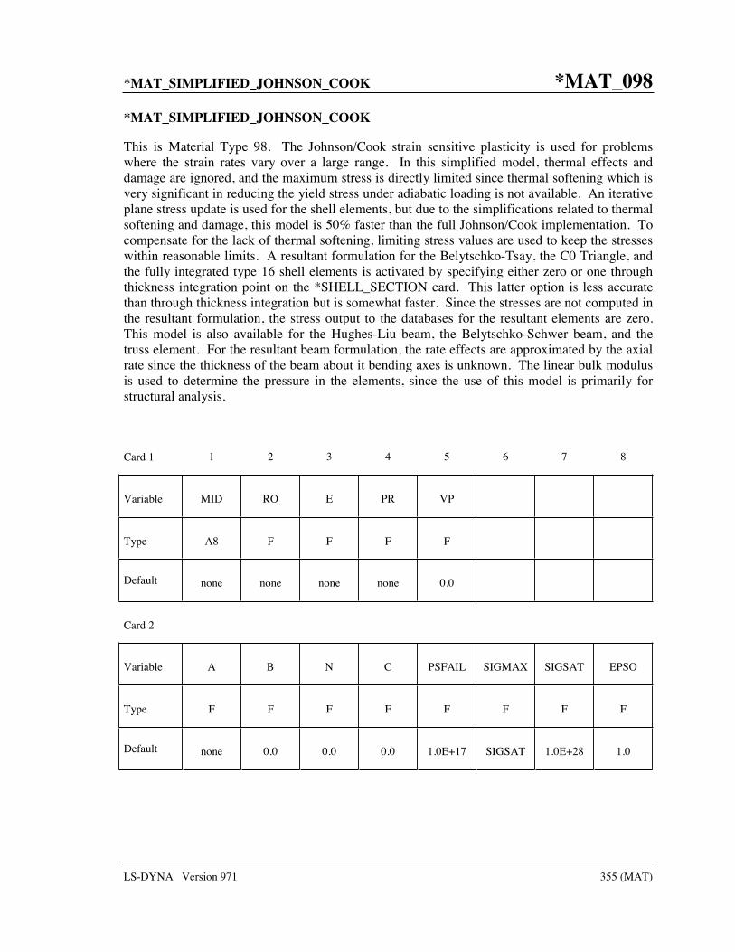
*MAT_SIMPLIFIED_JOHNSON_COOK *MAT_098
LS-DYNA Version 971 355 (MAT)
*MAT_SIMPLIFIED_JOHNSON_COOK
This is Material Type 98. The Johnson/Cook strain sensitive plasticity is used for problems where the strain rates vary over a large range. In this simplified model, thermal effects and damage are ignored, and the maximum stress is directly limited since thermal softening which is very significant in reducing the yield stress under adiabatic loading is not available. An iterative plane stress update is used for the shell elements, but due to the simplifications related to thermal softening and damage, this model is 50% faster than the full Johnson/Cook implementation. To compensate for the lack of thermal softening, limiting stress values are used to keep the stresses within reasonable limits. A resultant formulation for the Belytschko-Tsay, the C0 Triangle, and the fully integrated type 16 shell elements is activated by specifying either zero or one through thickness integration point on the *SHELL_SECTION card. This latter option is less accurate than through thickness integration but is somewhat faster. Since the stresses are not computed in the resultant formulation, the stress output to the databases for the resultant elements are zero. This model is also available for the Hughes-Liu beam, the Belytschko-Schwer beam, and the truss element. For the resultant beam formulation, the rate effects are approximated by the axial rate since the thickness of the beam about it bending axes is unknown. The linear bulk modulus is used to determine the pressure in the elements, since the use of this model is primarily for structural analysis.
Card 1 1 2 3 4 5 6 7 8
Variable MID RO E PR VP
Type A8 F F F F
Default none none none none 0.0
Card 2
Variable A B N C PSFAIL SIGMAX SIGSAT EPSO
Type F F F F F F F F
Default none 0.0 0.0 0.0 1.0E+17 SIGSAT 1.0E+28 1.0

*MAT_098 *MAT_SIMPLIFIED_JOHNSON_COOK
356 (MAT) LS-DYNA Version 971
VARIABLE DESCRIPTION
MID Material identification. A unique number or label not exceeding 8 characters must be specified.
RO Mass density
E Young’s modulus
PR Poisson’s ratio
VP Formulation for rate effects: EQ.0.0: Scale yield stress (default), EQ.1.0: Viscoplastic formulation. This option applies only to the 4-node shell and 8-node thick shell if and
only if through thickness integration is used.
A See equations below.
B See equations below.
N See equations below.
C See equations below.
PSFAIL Effective plastic strain at failure. If zero failure is not considered.
SIGMAX Maximum stress obtainable from work hardening before rate effects are added (optional). This option is ignored if VP=1.0. This option is ignored if VP=1.0.
SIGSAT Saturation stress which limits the maximum value of effective stress which can develop after rate effects are added (optional).
εPSO Strain rate normalization factor. This value depends on the time units. Typically, input 1 for units of seconds, 0.001 for units of milliseconds, 0.000001 for microseconds, etc.
Remarks:
Johnson and Cook express the flow stress as
( ) 1 ln *np
y A B cσ ε ε= + +
where
A, B, C and n are input constants pε effective plastic strain

*MAT_SIMPLIFIED_JOHNSON_COOK *MAT_098
LS-DYNA Version 971 357 (MAT)
0
εεε
∗ = effective strain rate for 10 1 sε −=
The maximum stress is limited by sigmax and sigsat by:
min , 1 ln * ,np
y min A B sigmax c sigsatσ ε ε= + +
Failure occurs when the effective plastic strain exceeds psfail.
If the viscoplastic option is active, VP=1.0, the parameters SIGMAX and SIGSAT are ignored since these parameters make convergence of the viscoplastic strain iteration loop difficult to achieve. The viscoplastic option replaces the plastic strain in the forgoing equations by the viscoplastic strain and the strain rate by the viscoplastic strain rate. Numerical noise is substantially reduced by the viscoplastic formulation.

*MAT_099 *MAT_SIMPLIFIED_JOHNSON_COOK_ORTHOTROPIC_DAMAGE
358 (MAT) LS-DYNA Version 971
*MAT_SIMPLIFIED_JOHNSON_COOK_ORTHOTROPIC_DAMAGE
This is Material Type 99. This model, which is implemented with multiple through thickness integration points, is an extension of model 98 to include orthotropic damage as a means of treating failure in aluminum panels. Directional damage begins after a defined failure strain is reached in tension and continues to evolve until a tensile rupture strain is reached in either one of the two orthogonal directions. After rupture is detected at NUMINT integration points, the element is deleted.
Card 1 1 2 3 4 5 6 7 8
Variable MID RO E PR VP EPPFR LCDM NUMINT
Type A8 F F F F F I I
Default none none none none 0.0 1.e+16 optional all intg. pt
Card 2
Variable A B N C PSFAIL SIGMAX SIGSAT EPSO
Type F F F F F F F F
Default none 0.0 0.0 0.0 1.0E+17 SIGSAT 1.0E+28 1.0
VARIABLE DESCRIPTION
MID Material identification. A unique number or label not exceeding 8 characters must be specified.
RO Mass density
E Young’s modulus
PR Poisson’s ratio
VP Formulation for rate effects: EQ.0.0: Scale yield stress (default), EQ.1.0: Viscoplastic formulation. This option applies only to the 4-node shell and 8-node thick shell if and
only if through thickness integration is used.

*MAT_SIMPLIFIED_JOHNSON_COOK_ORTHOTROPIC_DAMAGE *MAT_099
LS-DYNA Version 971 359 (MAT)
VARIABLE DESCRIPTION
EPPFR Plastic strain at which material ruptures (logarithmic).
LCDM Load curve ID defining nonlinear damage curve. See Figure 81-82.2.
NUMINT Number of through thickness integration points which must fail before the element is deleted. (If zero, all points must fail.) The default of all integration points is not recommended since elements undergoing large strain are often not deleted due to nodal fiber rotations which limit 0strains at active integration points after most points have failed. Better results are obtained if NUMINT is set to 1 or a number less than one half of the number of through thickness points. For example, if four through thickness points are used, NUMINT should not exceed 2, even for fully integrated shells which have 16 integration points.
A See equations below.
B See equations below.
N See equations below.
C See equations below.
PSFAIL Principal plastic strain at failure. If zero failure is not considered.
SIGMAX Maximum stress obtainable from work hardening before rate effects are added (optional). This option is ignored if VP=1.0. This option is ignored if VP=1.0.
SIGSAT Saturation stress which limits the maximum value of effective stress which can develop after rate effects are added (optional).
εPSO Effective plastic strain rate. This value depends on the time units. Typically, input 1 for units of seconds, 0.001 for units of milliseconds, 0.000001 for microseconds, etc.
Remarks:
See the description for the SIMPLIFIED_JOHNSON_COOK model above.

*MAT_100 *MAT_SPOTWELD
360 (MAT) LS-DYNA Version 971
*MAT_SPOTWELD_{OPTION}
This is Material Type 100. The material model applies to beam element type 9 and to solid element type 1 with type 6 hourglass controls. The failure models apply to both beam and solid elements.
The beam elements, based on the Hughes-Liu beam formulation, may be placed between any two deformable shell surfaces and tied with constraint contact, *CONTACT_SPOTWELD, which eliminates the need to have adjacent nodes at spot weld locations. Beam spot welds may be placed between rigid bodies and rigid/deformable bodies by making the node on one end of the spot weld a rigid body node which can be an extra node for the rigid body, see *CONSTRAINED_ EXTRA_NODES_OPTION. In the same way rigid bodies may also be tied together with this spot weld option. This weld option should not be used with rigid body switching. The foregoing advice is valid if solid element spot welds are used; however, since the solid elements have just three degrees-of-freedom at each node, *CONTACT_TIED_SURFACE_TO_SURFACE must be used instead of *CONTACT_SPOTWELD.
In flat topologies the shell elements have an unconstrained drilling degree-of-freedom which prevents torsional forces from being transmitted. If the torsional forces are deemed to be important, brick elements should be used to model the spot welds.
Beam and solid element force resultants for MAT_SPOTWELD are written to the spot weld force file, SWFORC, and the file for element stresses and resultants for designated elements, ELOUT.
It is advisable to include all spot welds, which provide the slave nodes, and spot welded materials, which define the master segments, within a single *CONTACT_SPOTWELD interface for beam element spot welds or a *CONTACT_TIED_SURFACE_TO_SURFACE interface for solid element spot welds. As a constraint method these interfaces are treated independently which can lead to significant problems if such interfaces share common nodal points. An added benefit is that memory usage can be substantially less with a single interface.
Available options include:
<BLANK>
DAMAGE-FAILURE
The DAMAGE-FAILURE option causes one additional line to be read with the damage parameter and a flag that determines how failure is computed from the resultants. On this line the parameter, RS, if nonzero, invokes damage mechanics combined with the plasticity model to achieve a smooth drop off of the resultant forces prior to the removal of the spot weld. The parameter OPT determines the method used in computing resultant based failure, which is unrelated to damage.

*MAT_SPOTWELD *MAT_100
LS-DYNA Version 971 361 (MAT)
Card 1 1 2 3 4 5 6 7 8
Variable MID RO E PR SIGY ET DT TFAIL
Type A8 F F F F F F F
Define this card as Card 2 when the DAMAGE-FAILURE option is inactive. Card 3 is not defined
Card 2 1 2 3 4 5 6 7 8
Variable EFAIL NRR NRS NRT MRR MSS MTT NF
Type F F F F F F F F
Define cards 2 and 3 below if the DAMAGE-FAILURE option is active. OPT=-1.0 and 0.0, Resultant based failure.
Card 2 1 2 3 4 5 6 7 8
Variable EFAIL NRR NRS NRT MRR MSS MTT NF
Type F F F F F F F F
OPT=1.0,.Stress based failure.
Card 2 1 2 3 4 5 6 7 8
Variable EFAIL SIGAX SIGTAU NF
Type F F F F

*MAT_100 *MAT_SPOTWELD
362 (MAT) LS-DYNA Version 971
OPT=1.0, Stress based failure if strain rate effects are included
Card 2 1 2 3 4 5 6 7 8
Variable EFAIL -LCAX -LCTAU NF
Type F F F F
OPT=2.0, User subroutine for failure
Card 2 1 2 3 4 5 6 7 8
Variable EFAIL USERV1 USERV2 USERV3 USERV4 USERV5 USERV6 NF
Type F F F F F F F F
OPT=3.0, 4.0
Card 2 1 2 3 4 5 6 7 8
Variable EFAIL ZD ZT ZALP1 ZALP2 ZALP3 ZRRAD NF
Type F F F F F F F F
OPT=5.0
Card 2 1 2 3 4 5 6 7 8
Variable EFAIL ZD ZT ZT2
Type F F F F
OPT=6.0, 7.0, and 9.0
Card 2 1 2 3 4 5 6 7 8
Variable EFAIL NF
Type F F

*MAT_SPOTWELD *MAT_100
LS-DYNA Version 971 363 (MAT)
Card 3 is defined only for the DAMAGE-FAILURE option.
Card 3 1 2 3 4 5 6 7 8
Variable RS OPT FVAL TRUE_T BETA
Type F F F F F
VARIABLE DESCRIPTION
MID Material identification. A unique number or label not exceeding 8 characters must be specified.
RO Mass density
E Young’s modulus
PR Poisson’s ratio
SIGY Initial yield stress
ET Hardening modulus, Et
DT Time step size for mass scaling, Δt
TFAIL Failure time if nonzero. If zero this option is ignored.
EFAIL Effective plastic strain in weld material at failure. If the damage option is inactive, the spot weld element is deleted when the plastic strain at each integration point exceeds EFAIL. If the damage option is active, the plastic strain must exceed the rupture strain at each integration point before deletion occurs.
NRR Axial force resultant FrrN or maximum axial stress F
rrσ at failure
depending on the value of OPT (see below). If zero, failure due to this component is not considered. If negative, |NRR| is the load curve ID defining the maximum axial stress at failure as a function of the effective strain rate.
NRS Force resultant FrsN or maximum shear stress Fτ at failure depending
on the value of OPT (see below). If zero, failure due to this component is not considered. If negative, |NRS| is the load curve ID defining the maximum shear stress at failure as a function of the effective strain rate.

*MAT_100 *MAT_SPOTWELD
364 (MAT) LS-DYNA Version 971
VARIABLE DESCRIPTION
NRT Force resultant FrtN at failure. If zero, failure due to this component is
not considered.
MRR Torsional moment resultant FrrM at failure. If zero, failure due to this
component is not considered.
MSS Moment resultant FssM at failure. If zero, failure due to this component
is not considered.
MTT Moment resultant FttM at failure. If zero, failure due to this component
is not considered.
NF Number of force vectors stored for filtering. The default value is set to zero which is generally recommended unless oscillatory resultant forces are observed in the time history databases. Even though these welds should not oscillate significantly, this option was added for consistency with the other spot weld options. NF affects the storage since it is necessary to store the resultant forces as history variables. When NF is nonzero, the resultants in the output databases are filtered. NF cannot exceed 30.
SIGAX Maximum axial stress σ rrF at failure. If zero, failure due to this
component is not considered.
SIGTAU Maximum shear stress τ F at failure. If zero, failure due to this
component is not considered.
LCAX Load curve ID defining the maximum axial stress at failure as a function of the effective strain rate. Input as a negative number.
LCTAU Load curve ID defining the maximum shear stress at failure as a function of the effective strain rate. Input as a negative number.
USERVn Failure constants for user failure subroutine, n=1,2,...6.
ZD Notch diameter
ZT Sheet thickness.
ZALP1 Correction factor alpha1
ZALP2 Correction factor alpha2
ZALP3 Correction factor alpha3

*MAT_SPOTWELD *MAT_100
LS-DYNA Version 971 365 (MAT)
VARIABLE DESCRIPTION
ZRRAD Notch root radius (OPT=3.0 only).
ZT2 Second sheet thickness (OPT = 5.0 only)
RS Rupture strain. Define if and only if damage is active.
OPT Failure option: EQ.-2: same as option –1 but in addition, the peak value of the
failure criteria and the time it occurs is stored and is written into the SWFORC database. This information may be necessary since the instantaneous values written at specified time intervals may miss the peaks. Additional storage is allocated to store this information.
EQ.-1: resultant based failure criteria, FC, is computed based on the force and moment resultants and is written into the SWFORC file. Failure is not allowed. This allows easy identification of vulnerable spot welds in the post-processing. Failure is likely to occur if FC >1.0. Only the terms where the corresponding failure resultant is nonzero are included when FC is calculated. This option applies to both solid and beam elements.
( )2 2 2 2 2 2
,0
F F F F F F
rr rs rt rr ss tt
rr rs rt rr ss tt
max N N N M M MFC
N N N M M M= + + + + +
EQ. 0: resultant based failure EQ. 1: stress based failure computed from resultants (Toyota) EQ. 2: user subroutine to determine failure EQ. 3: notch stress based failure (beam weld only) EQ. 4: stress intensity factor at failure (beam weld only) EQ. 5: structural stress at failure (beam weld only). EQ. 6: stress based failure computed from resultants (Toyota). In
this option a shell strain rate dependent failure model is used (beam weld only). The static failure stresses are defined by part ID using the input given in the keyword definition *DEFINE_SPOTWELD_ RUPTURE_STRESS input.
EQ. 7: stress based failure for solid elements (Toyota) with peak stresses computed from resultants, and strength values input for pairs of parts, see *DEFINE_SPOTWELD_FAILURE_ RESULTANTS. Strain rate effects are optional.
EQ. 8: Not used. EQ. 9: Stress based failure from resultants (Toyota). In this option a
shell strain rate dependent failure model is used (beam weld only). The static failure stresses are defined by part ID using the input given in the keyword definition *DEFINE_SPOTWELD_ RUPTURE_PARAMETER input.

*MAT_100 *MAT_SPOTWELD
366 (MAT) LS-DYNA Version 971
VARIABLE DESCRIPTION
FVAL Failure parameter. If OPT: EQ.-2: Not used. EQ.-1: Not used. EQ. 0: Not used. EQ. 1: Not used. EQ. 2: Not used. EQ. 3: Notch stress value at failure (σKF). EQ. 4: Stress intensity factor value at failure (KeqF). EQ. 5: Structural stress value at failure (σsF). EQ. 6: Number of cycles that failure condition must be met to
trigger beam deletion. EQ. 7: Not used. EQ. 9: Number of cycles that failure condition must be met to
trigger beam deletion.
TRUE_T True weld thickness. This optional value is available for solid element failure by OPT=0,1,7, or –2. TRUE_T is used to reduce the moment contribution to the failure calculation from artificially thick weld elements so shear failure can be modeled more accurately. See comments under the remarks for *MAT_SPOTWELD_DAIMLER CHRYSLER
BETA Damage model decay rate.
Remarks:
The weld material is modeled with isotropic hardening plasticity coupled to failure models. EFAIL specifies a failure strain which fails each integration point in the spot weld independently. The resultant-based failure model fails the entire weld if the resultants are outside of the failure surface defined by:
( )2 2 2 2 2 2
,01 0
F F F F F F
rr rs rt rr ss tt
rr rs rt rr ss tt
max N N N M M M
N N N M M M+ + + + + − =
where the numerators in the equation are the resultants calculated in the local coordinates of the cross section, and the denominators are the values specified in the input. If NF is nonzero the resultants are filtered before failure is checked. The stress based failure model (OPT=1), which was developed by Toyota Motor Corporation and is based on the peak axial and transverse shear stresses, fails the entire weld if the stresses are outside of the failure surface defined by
2 2
1 0rrF Frr
σ τσ τ
+ − =
*MAT_SPOTWELD *MAT_100
LS-DYNA Version 971 367 (MAT)
If strain rates are considered then the failure criteria becomes:
( ) ( )
2 2
1 0rrF Frr eff eff
σ τσ ε τ ε
+ − =
where ( )Frr effσ ε and ( )F
effτ ε are defined by load curves LCAX and LCTAU. The peak stresses
are calculated from the resultants using simple beam theory.
2 2 2 2
2ss tt rs rtrr rr
rr
M M N NN M
A Z Z Aσ τ
+ += + = +
where the area and section modulus are given by:
2
3
4
32
dA
dZ
π
π
=
=
and d is the equivalent diameter of the beam element or solid element used as a spot weld.
OPT=2 invokes a user-written subroutine uweldfail, documented in Appendix Q.
The failure based on notch stress (OPT=3), see Zhang [1999], occurs when the failure criterion:
0k kFσ σ− ≥
is satisfied. The notch stress is give by the equation:
1 2 32 2
4 3 19 6 2 4 51 1 1
8 3 3 2rr
k
F t M t F d t
dt dt d tσ α α α
π ρ π ρ π ρπ π π+= + + + + +
Here,
2 2
2 2
rs rt
ss tt
F F F
M M M
= +
= +
and αi i =1,2,3 are input corrections factors with default values of unity. If spot welds are between sheets of unequal thickness, the minimum thickness of the spot welded sheets may be introduced as a crude approximation.
The failure based on structural stress intensity (OPT=4) occurs, see Zhang [1999], when the failure criterion:
0eq eqFK K− ≥

*MAT_100 *MAT_SPOTWELD
368 (MAT) LS-DYNA Version 971
is satisfied where 2 2
eq I IIK K K= +
and
1 2 3
1
3 2 3 5 2
2 32
rrI
II
F M FK
d t dt t d tF
Kd t
α α απ π π
απ
= + +
=
Here, F and M are as defined above for the notch stress formulas and again, αi i =1,2,3 are input corrections factors with default values of unity. If spot welds are between sheets of unequal thickness, the minimum thickness of the spot welded sheets may be used as a crude approximation.
The maximum structural stress at the spot weld was utilized successfully for predicting the fatigue failure of spot welds, see Rupp, et. al. [1994] and Sheppard [1993]. The corresponding results according to Rupp, et. al. are listed below where it is assumed that they may be suitable for crash conditions.
The failure criterion invoked by OPT=5 is given by:
( )1 2 3max , , 0v v v sFσ σ σ σ− =
where σsF is the critical value of structural stress at failure. It is noted that the forces and moments in the equations below are referred to the beam nodes 1, 2, and to the midpoint, respectively. The three stress values, σv1,σv 2,σv3 , are defined by:
( ) 1 1 1 1 1 11
1 1 1 1 1 1 1 1
1.046 1.123 1.123cos sin sin cosrs rt rr ss tt
v
F F F M M
dt dt t t dt t dt t
βσ ζ ζ ζ ζ ζπ π
= + − − + with
1 1
1 1
0 0
1 0rr
rr
if F
if F
ββ
= ≤= >
( ) 2 2 1 2 2 22
2 2 2 2 2 2 2 2
1.046 1.123 1.123cos sin sin cosrs rt rr ss tt
v
F F F M M
dt dt t t dt t dt t
βσ ζ ζ ζ ζ ζπ π
= + − + − with
2 2
2 2
0 0
1 0rr
rr
if F
if F
ββ
= ≤= >
( ) ( ) ( ) ( ) ( ) ( )3 0.5 0.5 cos 2 0.5 sin 2vσ ζ σ ζ σ ζ α τ ζ α= + +

*MAT_SPOTWELD *MAT_100
LS-DYNA Version 971 369 (MAT)
where
( )
( )
( )( )
32 3 3
2 22 2
1
4 32 32sin cos
16 16sin cos
3 321
tan2
rr ss tt
rs rt
F M M
d d dF F
d d
βσ ζ ζ ζπ π π
τ ζ ζ ζπ π
τ ζα
σ ζ−
= + −
= +
=
with 3
3
0 0
1 0rr
rr
if F
if F
ββ
= ≤= >
The stresses are calculated for all directions, 0° ≤ζ ≤ 90° , in order to find the maximum.
If the failure strain EFAIL is set to zero, the failure strain model is not used. In a similar manner, when the value of a resultant at failure is set to zero, the corresponding term in the failure surface is ignored. For example, if only NrrF
is nonzero, the failure surface is reduced to
Frr rrN N= . None, either, or both of the failure models may be active depending on the specified
input values.
The inertias of the spot welds are scaled during the first time step so that their stable time step size is Δt. A strong compressive load on the spot weld at a later time may reduce the length of the spot weld so that stable time step size drops below Δt. If the value of Δt is zero, mass scaling is not performed, and the spot welds will probably limit the time step size. Under most circumstances, the inertias of the spot welds are small enough that scaling them will have a negligible effect on the structural response and the use of this option is encouraged.
Spot weld force history data is written into the SWFORC ascii file. In this database the resultant moments are not available, but they are in the binary time history database and in the ASCII elout file.
When the DAMAGE-FAILURE option is invoked, the constitutive properties for the damaged material are obtained from the undamaged material properties. The amount of damage evolved is represented by the constant, ω , which varies from zero if no damage has occurred to unity for complete rupture. For uniaxial loading, the nominal stress in the damaged material is given by
nominal
P
Aσ =
where P is the applied load and A is the surface area. The true stress is given by:
trueloss
P
A Aσ =
−
where Aloss is the void area. The damage variable can then be defined:
lossA
Aω = 0 1ω≤ ≤

*MAT_100 *MAT_SPOTWELD
370 (MAT) LS-DYNA Version 971
In this model damage is defined in terms of plastic strain after the failure strain is exceeded:
p peff failure p p p
failure eff rupturep prupture failure
ifε ε
ω ε ε εε ε
−= ≤ ≤
−
After exceeding the failure strain EFAIL, softening begins and continues until the rupture strain RS is reached.
If BETA is specified, the stress is multiplied by an exponential using ω defined in the previous equation,
exp(- )dσ σ βω= ⋅ .
Figure 100.1. A solid element used as spot weld is shown. When resultant based failure is used orientation is very important. Nodes n1-n4 attach to the lower shell mid-surface and nodes n5-n8 attach to the upper shell mid-surface. The resultant forces and moments are computed based on the assumption that the brick element is properly oriented.

*MAT_SPOTWELD_DAIMLERCHRYSLER *MAT_100_DA
LS-DYNA Version 971 371 (MAT)
*MAT_SPOTWELD_DAIMLERCHRYSLER
This is Material Type 100. The material model applies to solid element type 1 with type 6 hourglass control. Spot weld elements may be placed between any two deformable shell surfaces and tied with constraint contact, *CONTACT_TIED_SURFACE_TO_SURFACE, which eliminates the need to have adjacent nodes at spot weld locations. Spot weld failure is modeled using this card and *DEFINE_CONNECTION_PROPERTIES data. Details of the failure model can be found in Seeger, Feucht, Frank, Haufe, and Keding [2005].
It is advisable to include all spot welds, which provide the slave nodes, and spot welded materials, which define the master segments, within a single *CONTACT_TIED_ SURFACE_TO_SURFACE interface. This contact type uses constraint equations. If multiple interfaces are treated independently, significant problems can occur if such interfaces share common nodes. An added benefit is that memory usage can be substantially less with a single interface.
Card 1 1 2 3 4 5 6 7 8
Variable MID RO E PR DT TFAIL
Type A8 F F F F F
Card 2
Variable EFAIL NF
Type F F
Card 3
Variable RS TRUE_T CON_ID
Type F F F

*MAT_100_DA *MAT_SPOTWELD_DAIMLERCHRYSLER
372 (MAT) LS-DYNA Version 971
VARIABLE DESCRIPTION
MID Material identification. A unique number or label not exceeding 8 characters must be specified.
RO Mass density.
E Young’s modulus.
PR Poisson’s ratio.
DT Time step size for mass scaling, Δt.
TFAIL Failure time if nonzero. If zero this option is ignored.
EFAIL Effective plastic strain in weld material at failure. See remark below.
NF Number of failure function evaluations stored for filtering by time averaging. The default value is set to zero which is generally recommended unless oscillatory resultant forces are observed in the time history databases. Even though these welds should not oscillate significantly, this option was added for consistency with the other spot weld options. NF affects the storage since it is necessary to store the failure terms. When NF is nonzero, the resultants in the output databases are filtered. NF cannot exceed 30.
RS Rupture strain. See Remarks below.
TRUE_T True weld thickness for single hexahedron solid weld elements. See comments below.
CON_ID Connection ID of *DEFINE_CONNECTION card.
Remarks:
This weld material is modeled with isotropic hardening plasticity. The yield stress and constant hardening modulus are assumed to be those of the welded shell elements as defined in a *DEFINE_CONNECTION_PROPERTIES table. A failure function and damage type is also defined by *DEFINE_ CONNECTION_PROPERTIES data. The interpretation of EFAIL and RS is determined by the choice of damage type. This is discussed in remark 4 on *DEFINE_CONNECTION_PROPERTIES.
Solid weld elements are tied to the mid-plane of shell materials and so typically have a thickness that is half the sum of the thicknesses of the welded shell sections. As a result, a weld under shear loading can be subject to an artificially large moment which will be balanced by normal forces transferred through the tied contact. These normal forces will cause the normal term in the failure calculation to be artificially high. Inputting a TRUE_T that is smaller than the modeled thickness, for example, 10%-30% of true thickness, will scale down the normal force

*MAT_SPOTWELD_DAIMLERCHRYSLER *MAT_100_DA
LS-DYNA Version 971 373 (MAT)
that results from the balancing moment and provide more realistic failure calculations. TRUE_T effects only the failure calculation, not the weld element behavior. If TRUE_T=0 or data is omitted, the modeled weld element thickness is used.
Solid element force resultants for MAT_SPOTWELD are written to the spot weld force file, SWFORC, and the file for element stresses and resultants for designated elements, ELOUT. Also, spot weld failure data is written to the file, DCFAIL.

*MAT_101 *MAT_GEPLASTIC_SRATE_2000a
374 (MAT) LS-DYNA Version 971
*MAT_GEPLASTIC_SRATE_2000a
This is Material Type 101. The GEPLASTIC_SRATE_2000a material model characterizes General Electric's commercially available engineering thermoplastics subjected to high strain rate events. This material model features the variation of yield stress as a function of strain rate, cavitation effects of rubber modified materials and automatic element deletion of either ductile or brittle materials.
Card 1 1 2 3 4 5 6 7 8
Variable MID RO E PR RATESF EDOT0 ALPHA
Type A8 F F F F F F
Card 2
Variable LCSS LCFEPS LCFSIG LCE
Type F F F F
VARIABLE DESCRIPTION
MID Material identification. A unique number or label not exceeding 8 characters must be specified.
RO Mass density.
E Young's Modulus.
PR Poisson's ratio.
RATESF Constant in plastic strain rate equation.
EDOT0 Reference strain rate
ALPHA Pressure sensitivity factor
LCSS Load curve ID or Table ID that defines the post yield material behavior. The values of this stress-strain curve are the difference of the yield stress and strain respectively. This means the first values for both stress and strain should be zero. All subsequent values will define softening or hardening.

*MAT_GEPLASTIC_SRATE_2000a *MAT_101
LS-DYNA Version 971 375 (MAT)
VARIABLE DESCRIPTION
LCFEPS Load curve ID that defines the plastic failure strain as a function of strain rate.
LCFSIG Load curve ID that defines the Maximum principal failure stress as a function of strain rate.
LCE Load curve ID that defines the Unloading moduli as a function of plastic strain.
Remarks:
The constitutive model for this approach is:
0 exp( { ( )}) exp( )p pA S p Aσ αε ε ε= − × −
where 0ε and A are rate dependent yield stress parameters, ( )pS ε internal resistance (strain hardening) and α is a pressure dependence parameter.
In this material the yield stress may vary throughout the finite element model as a function of strain rate and hydrostatic stress. Post yield stress behavior is captured in material softening and hardening values. Finally, ductile or brittle failure measured by plastic strain or maximum principal stress respectively is accounted for by automatic element deletion.
Although this may be applied to a variety of engineering thermoplastics, GE Plastics have constants available for use in a wide range of commercially available grades of their engineering thermoplastics.

*MAT_102 *MAT__INV_HYPERBOLIC_SIN
376 (MAT) LS-DYNA Version 971
*MAT_INV_HYPERBOLIC_SIN
This is Material Type 102. It allows the modeling of temperature and rate dependent plasticity, Sheppard and Wright [1979].
Card 1 1 2 3 4 5 6 7 8
Variable MID RO E PR T HC VP
Type A8 F F F F F F
Card 2
Variable ALPHA N A Q G EPS0
Type F F F F F F
VARIABLE DESCRIPTION
MID Material identification. A unique number or label not exceeding 8 characters must be specified.
RO Mass density.
E Young's Modulus.
PR Poisson's ratio
T Initial Temperature.
HC Heat generation coefficient.
VP Formulation for rate effects: EQ.0.0: Scale yield stress (default) EQ.1.0: Viscoplastic formulation.
ALPHA See Remarks.
N See Remarks.
A See Remarks.
Q See Remarks.
G See Remarks.

*MAT_INV_HYPERBOLIC_SIN *MAT_102
LS-DYNA Version 971 377 (MAT)
Remarks:
Resistance to deformation is both temperature and strain rate dependent. The flow stress equation is:
1
11sinh
NZ
Aσ
α−=
where Z , the Zener-Holloman temperature compensated strain rate, is:
expQ
ZGT
ε=
The units of the material constitutive constants are as follows: A (1/sec), N(dimensionless), α (1/MPa), the activation energy for flow, Q (J/mol), and the universal gas constant, G (J/mol K). The value of G will only vary with the unit system chosen. Typically it will be either 8.3144 J/mol ∞ K, or 40.8825 lb in/mol ∞ R.
The final equation necessary to complete our description of high strain rate deformation is one that allows us to compute the temperature change during the deformation. In the absence of a couples thermo-mechanical finite element code we assume adiabatic temperature change and follow the empirical assumption that 90-95% of the plastic work is dissipated as heat. Thus the heat generation coefficient is
0.9
v
HCCρ
≈
where ρ is the density of the material and Cv is the specific heat.

*MAT_103 *MAT_ANISOTROPIC_VISCOPLASTIC
378 (MAT) LS-DYNA Version 971
*MAT_ANISOTROPIC_VISCOPLASTIC
This is Material Type 103. This anisotropic-viscoplastic material model applies to shell and brick elements. The material constants may be fit directly or, if desired, stress versus strain data may be input and a least squares fit will be performed by LS-DYNA to determine the constants. Kinematic or isotopic or a combination of kinematic and isotropic hardening may be used. A detailed description of this model can be found in the following references: Berstad, Langseth, and Hopperstad [1994]; Hopperstad and Remseth [1995]; and Berstad [1996]. Failure is based on effective plastic strain or by a user defined subroutine.
Card 1 1 2 3 4 5 6 7 8
Variable MID RO E PR SIGY FLAG LCSS ALPHA
Type A8 F F F F F F F
Card 2
Variable QR1 CR1 QR2 CR2 QX1 CX1 QX2 CX2
Type F F F F F F F F
Card 3
Variable VK VM R00 or F R45 or G R90 or H L M N
Type F F F F F F F F
Card 4
Variable AOPT FAIL NUMINT MACF
Type F F F I

*MAT_ANISOTROPIC_VISCOPLASTIC *MAT_103
LS-DYNA Version 971 379 (MAT)
Card 5 1 2 3 4 5 6 7 8
Variable XP YP ZP A1 A2 A3
Type F F F F F F
Card 6
Variable V1 V2 V3 D1 D2 D3 BETA
Type F F F F F F F
VARIABLE DESCRIPTION
MID Material identification. A unique number or label not exceeding 8 characters must be specified.
RO Mass density.
E Young’s modulus
PR Poisson’s ratio
SIGY Initial yield stress
FLAG Flag EQ.0: Give all material parameters EQ.1: Material parameters are fit in LS-DYNA to Load curve or
Table given below. The parameters Qr1 , Cr1, Qr 2 , and Cr2 for isotropic hardening are determined by the fit and those for kinematic hardening are found by scaling those for isotropic hardening by . 1 − α( ) where α is defined below in columns 51-60.
EQ.2: Use load curve directly, i.e., no fitting is required for the parameters Qr1 , Cr1, Qr 2 , and Cr2 . A table is not allowed.
LCSS Load curve ID or Table ID. The load curve ID defines effective stress versus effective plastic strain. Card 2 is ignored with this option. The table ID, see Figure 24.1, defines for each strain rate value a load curve ID giving the stress versus effective plastic strain for that rate. If the load curve only is used, then the coefficients Vk and Vm must be given if viscoplastic behavior is desired. If a Table ID is given these coefficients are determined internally during initialization.

*MAT_103 *MAT_ANISOTROPIC_VISCOPLASTIC
380 (MAT) LS-DYNA Version 971
VARIABLE DESCRIPTION
ALPHA α distribution of hardening used in the curve-fitting. α = 0 pure kinematic hardening and α =1 provides pure isotropic hardening
QR1 Isotropic hardening parameter Qr1
CR1 Isotropic hardening parameter Cr1
QR2 Isotropic hardening parameter Qr 2
CR2 Isotropic hardening parameter Cr2
QX1 Kinematic hardening parameter Qχ1
CX1 Kinematic hardening parameter Cχ1
QX2 Kinematic hardening parameter Qχ 2
CX2 Kinematic hardening parameter Cχ 2
VK Viscous material parameter Vk
VM Viscous material parameter Vm
R00 R00 for shell (Default=1.0)
R45 R45 for shell (Default=1.0)
R90 R90 for shell (Default=1.0)
F F for brick (Default =1/2)
G G for brick (Default =1/2)
H H for brick (Default =1/2)
L L for brick (Default =3/2)
M M for brick (Default =3/2)
N N for brick (Default =3/2)

*MAT_ANISOTROPIC_VISCOPLASTIC *MAT_103
LS-DYNA Version 971 381 (MAT)
VARIABLE DESCRIPTION
AOPT Material axes option (see MAT_OPTION TROPIC_ELASTIC for a more complete description):
EQ.0.0: locally orthotropic with material axes determined by element nodes 1, 2, and 4, as with *DEFINE_COORDINATE_ NODES.
EQ.1.0: locally orthotropic with material axes determined by a point in space and the global location of the element center; this is the a-direction. This option is for solid elements only.
EQ.2.0: globally orthotropic with material axes determined by vectors defined below, as with *DEFINE_COORDINATE_ VECTOR.
EQ.3.0: locally orthotropic material axes determined by rotating the material axes about the element normal by an angle, BETA, from a line in the plane of the element defined by the cross product of the vector v with the element normal.
EQ.4.0: locally orthotropic in cylindrical coordinate system with the material axes determined by a vector v, and an originating point, P, which define the centerline axis. This option is for solid elements only.
LT.0.0: the absolute value of AOPT is a coordinate system ID number (CID on *DEFINE_COORDINATE_NODES, *DEFINE_ COORDINATE_SYSTEM or *DEFINE_COORDINATE_ VECTOR). Available in R3 version of 971 and later.
FAIL Failure flag. LT.0.0: User defined failure subroutine is called to determine
failure. This is subroutine named, MATUSR_103, in DYN21.F. EQ.0.0: Failure is not considered. This option is recommended if
failure is not of interest since many calculations will be saved. GT.0.0: Plastic strain to failure. When the plastic strain reaches
this value, the element is deleted from the calculation.
NUMINT Number of integration points which must fail before element deletion. If zero, all points must fail. This option applies to shell elements only. For the case of one point shells, NUMINT should be set to a value that is less than the number of through thickness integration points. Nonphysical stretching can sometimes appear in the results if all integration points have failed except for one point away from the midsurface. This is due to the fact that unconstrained nodal rotations will prevent strains from developing at the remaining integration point. In fully integrated shells, similar problems can occur.

*MAT_103 *MAT_ANISOTROPIC_VISCOPLASTIC
382 (MAT) LS-DYNA Version 971
VARIABLE DESCRIPTION
MACF Material axes change flag for brick elements: EQ.1: No change, default, EQ.2: switch material axes a and b, EQ.3: switch material axes a and c, EQ.4: switch material axes b and c.
XP,YP,ZP xp yp zp, define coordinates of point p for AOPT = 1 and 4.
A1,A2,A3 a1 a2 a3, define components of vector a for AOPT = 2.
V1,V2,V3 v1 v2 v3, define components of vector v for AOPT = 3 and 4.
D1,D2,D3 d1 d2 d3, define components of vector d for AOPT = 2.
BETA Μaterial angle in degrees for AOPT = 3, may be overridden on the element card, see *ELEMENT_SHELL_BETA or *ELEMENT_ SOLID_ORTHO.
Remarks:
The uniaxial stress-strain curve is given on the following form
0 1 1 2 2
1 1 2 2
( , ) (1 exp( )) (1 exp( ))
(1 exp( )) (1 exp( ))
m
p p p peff eff r r eff r r eff
p peff eff
Vpk eff
Q C Q C
Q C Q C
V
χ χ χ χ
σ ε ε σ ε ε
ε ε
ε
= + − − + − −
+ − − + − −
+
For bricks the following yield criteria is used
2 2 222 33 33 11 11 22
2 2 223 31 12
( ) ( ) ( )
2 2 2 ( , )p peff eff
F G H
L M N
σ σ σ σ σ σσ σ σ σ ε ε
− + − + −
+ + + =
where εeffp is the effective plastic strain and p
effε is the effective plastic strain rate. For shells the
anisotropic behavior is given by R00 , R45 and R90 . The model will work when the three first parameters in card 3 are given values. When Vk = 0 the material will behave elasto-plastically. Default values are given by:
1
2F G H= = =
3
2L M N= = =
R00 = R45 = R90 =1

*MAT_ANISOTROPIC_VISCOPLASTIC *MAT_103
LS-DYNA Version 971 383 (MAT)
Strain rate of accounted for using the Cowper and Symonds model which, e.g., model 3, scales the yield stress with the factor:
1
1pp
eff
C
ε+
To convert these constants set the viscoelastic constants, Vk and Vm , to the following values:
1
1
1
p
k
m
VC
Vp
σ=
=
This model properly treats rate effects. The viscoplastic rate formulation is an option in other plasticity models in LS-DYNA, e.g., mat_3 and mat_24, invoked by setting the parameter VP to 1.

*MAT_103_P *MAT_ANISOTROPIC_PLASTIC
384 (MAT) LS-DYNA Version 971
*MAT_ANISOTROPIC_PLASTIC
This is Material Type 103. This anisotropic-plastic material model is a simplified version of the MAT_ANISOTROPIC_VISCOPLASTIC above. This material model applies only to shell elements.
Card 1 1 2 3 4 5 6 7 8
Variable MID RO E PR SIGY LCSS
Type A8 F F F F F
Card 2
Variable QR1 CR1 QR2 CR2
Type F F F F
Card 3
Variable R00 R45 R90 S11 S22 S33 S12
Type F F F F F F F
Card 4
Variable AOPT
Type F

*MAT_ANISOTROPIC_PLASTIC *MAT_103_P
LS-DYNA Version 971 385 (MAT)
Card 5 1 2 3 4 5 6 7 8
Variable XP YP ZP A1 A2 A3
Type F F F F F F
Card 6
Variable V1 V2 V3 D1 D2 D3 BETA
Type F F F F F F F
VARIABLE DESCRIPTION
MID Material identification. A unique number or label not exceeding 8 characters must be specified.
RO Mass density.
E Young’s modulus
PR Poisson’s ratio
SIGY Initial yield stress
LCSS Load curve ID. The load curve ID defines effective stress versus effective plastic strain. Card 2 is ignored with this option.
QR1 Isotropic hardening parameter Qr1
CR1 Isotropic hardening parameter Cr1
QR2 Isotropic hardening parameter Qr 2
CR2 Isotropic hardening parameter Cr2
R00 R00 for anisotropic hardening
R45 R45 for anisotropic hardening
R90 R90 for anisotropic hardening
S11 Yield stress in local x-direction. This input is ignored if R00 , R45 ,R90( )> 0 .

*MAT_103_P *MAT_ANISOTROPIC_PLASTIC
386 (MAT) LS-DYNA Version 971
VARIABLE DESCRIPTION
S22 Yield stress in local y-direction. This input is ignored if R00 , R45 ,R90( )> 0 .
S33 Yield stress in local z-direction. This input is ignored if R00 , R45 ,R90( )> 0 .
S12 Yield stress in local xy-direction. This input is ignored if R00 , R45 ,R90( )> 0 .
AOPT Material axes option (see MAT_OPTION TROPIC_ELASTIC for a more complete description):
EQ.0.0: locally orthotropic with material axes determined by element nodes 1, 2, and 4, as with *DEFINE_COORDINATE_ NODES.
EQ.1.0: locally orthotropic with material axes determined by a point in space and the global location of the element center; this is the a-direction. This option is for solid elements only.
EQ.2.0: globally orthotropic with material axes determined by vectors defined below, as with *DEFINE_COORDINATE_ VECTOR.
EQ.3.0: locally orthotropic material axes determined by rotating the material axes about the element normal by an angle, BETA, from a line in the plane of the element defined by the cross product of the vector v with the element normal.
EQ.4.0: locally orthotropic in cylindrical coordinate system with the material axes determined by a vector v, and an originating point, P, which define the centerline axis. This option is for solid elements only.
LT.0.0: the absolute value of AOPT is a coordinate system ID number (CID on *DEFINE_COORDINATE_NODES, *DEFINE_ COORDINATE_SYSTEM or *DEFINE_COORDINATE_ VECTOR). Available in R3 version of 971 and later.
XP,YP,ZP xp yp zp, define coordinates of point p for AOPT = 1 and 4.
A1,A2,A3 a1 a2 a3, define components of vector a for AOPT = 2.
D1,D2,D3 d1 d2 d3, define components of vector d for AOPT = 2.
V1,V2,V3 v1 v2 v3, define components of vector v for AOPT = 3 and 4.
BETA Μaterial angle in degrees for AOPT = 3, may be overridden on the element card, see *ELEMENT_SHELL_BETA or *ELEMENT_ SOLID_ORTHO.

*MAT_ANISOTROPIC_PLASTIC *MAT_103_P
LS-DYNA Version 971 387 (MAT)
Remarks:
If no load curve is defined for the effective stress versus effective plastic strain, the uniaxial stress-strain curve is given on the following form
σ(εeffp ) = σ0 + Qr1(1 − exp(−Cr1εeff
p )) + Qr 2(1− exp(−Cr2εeffp ))
where εeffp is the effective plastic strain. For shells the anisotropic behavior is given by R00 , R45
and R90 , or the yield stress in the different direction. Default values are given by:
R00 = R45 = R90 =1
if the variables R00, R45, R90, S11, S22, S33 and S12 are set to zero.

*MAT_104 *MAT_DAMAGE_1
388 (MAT) LS-DYNA Version 971
*MAT_DAMAGE_1
This is Material Type 104. This is a continuum damage mechanics (CDM) model which includes anisotropy and viscoplasticity. The CDM model applies to shell, thick shell, and brick elements. A more detailed description of this model can be found in the paper by Berstad, Hopperstad, Lademo, and Malo [1999]. This material model can also model anisotropic damage behavior by setting the FLAG to -1 in Card 2.
Card 1 1 2 3 4 5 6 7 8
Variable MID RO E PR SIGY LCSS LCDS
Type A8 F F F F
Card 2
Variable Q1 C1 Q2 C2 EPSD S or EPSR DC FLAG
Type F F F F F F F F
Card 3
Variable VK VM R00 or F R45 or G R90 or H L M N
Type F F F F F F F F
Card 4
Variable AOPT MACF
Type F I

*MAT_DAMAGE_1 *MAT_104
LS-DYNA Version 971 389 (MAT)
Card 5 1 2 3 4 5 6 7 8
Variable XP YP ZP A1 A2 A3
Type F F F F F F
Card 6
Variable V1 V2 V3 D1 D2 D3 BETA
Type F F F F F F F
VARIABLE DESCRIPTION
MID Material identification. A unique number or label not exceeding 8 characters must be specified.
RO Mass density.
E Young’s modulus
PR Poisson’s ratio
SIGY Initial yield stress, σ0 .
LCSS Load curve ID. Load curve ID defining effective stress versus effective plastic strain. For FLAG = -1.
LCDS Load curve ID defining nonlinear damage curve. For FLAG = -1.
Q1 Isotropic hardening parameter Q1
C1 Isotropic hardening parameter C1
Q2 Isotropic hardening parameter Q2
C2 Isotropic hardening parameter C2
EPSD Damage threshold rd Damage effective plastic strain when material softening begin. (Default=0.0)
S Damage material constant S . (Default= 0
200
σ). For FLAG≥0.

*MAT_104 *MAT_DAMAGE_1
390 (MAT) LS-DYNA Version 971
VARIABLE DESCRIPTION
EPSR Plastic strain at which material ruptures (logarithmic).
DC Critical damage value DC . When the damage value D reaches this value, the element is deleted from the calculation. (Default=0.5) For FLAG≥0.
FLAG Flag EQ.-1: Anisotropic damage
EQ.0: No calculation of localization due to damage EQ.1: The model flags element where strain localization occur
VK Viscous material parameter Vk
VM Viscous material parameter Vm
R00 R00 for shell (Default=1.0)
R45 R45 for shell (Default=1.0)
R90 R90 for shell (Default=1.0)
F F for brick (Default =1/2)
G G for brick (Default =1/2)
H H for brick (Default =1/2)
L L for brick (Default =3/2)
M M for brick (Default =3/2)
N N for brick (Default =3/2)
AOPT Material axes option (see MAT_OPTION TROPIC_ELASTIC for a more complete description):
EQ.0.0: locally orthotropic with material axes determined by element nodes 1, 2, and 4, as with *DEFINE_COORDINATE_ NODES.
EQ.1.0: locally orthotropic with material axes determined by a point in space and the global location of the element center; this is the a-direction. This option is for solid elements only.
EQ.2.0: globally orthotropic with material axes determined by vectors defined below, as with *DEFINE_COORDINATE_ VECTOR.

*MAT_DAMAGE_1 *MAT_104
LS-DYNA Version 971 391 (MAT)
VARIABLE DESCRIPTION
EQ.3.0: locally orthotropic material axes determined by rotating the material axes about the element normal by an angle, BETA, from a line in the plane of the element defined by the cross product of the vector v with the element normal.
EQ.4.0: locally orthotropic in cylindrical coordinate system with the material axes determined by a vector v, and an originating point, P, which define the centerline axis. This option is for solid elements only.
LT.0.0: the absolute value of AOPT is a coordinate system ID number (CID on *DEFINE_COORDINATE_NODES, *DEFINE_ COORDINATE_SYSTEM or *DEFINE_COORDINATE_ VECTOR). Available in R3 version of 971 and later.
MACF Material axes change flag for brick elements: EQ.1: No change, default, EQ.2: switch material axes a and b, EQ.3: switch material axes a and c, EQ.4: switch material axes b and c.
XP,YP,ZP xp yp zp, define coordinates of point p for AOPT = 1 and 4.
A1,A2,A3 a1 a2 a3, define components of vector a for AOPT = 2.
D1,D2,D3 d1 d2 d3, define components of vector d for AOPT = 2.
V1,V2,V3 v1 v2 v3, define components of vector v for AOPT = 3 and 4.
BETA Μaterial angle in degrees for AOPT = 3, may be overridden on the element card, see *ELEMENT_SHELL_BETA or *ELEMENT_ SOLID_ORTHO.
Remarks:
Anisotropic Damage model (FLAG = -1). At each thickness integration points, an anisotropic damage law acts on the plane stress tensor in the directions of the principal total shell strains, ε1 and ε2 , as follows:
σ11 = (1 − D1 (ε1))σ110
σ22 = (1− D2 (ε2 ))σ 220
σ12 = (1− (D1 + D2 )/ 2)σ120
The transverse plate shear stresses in the principal strain directions are assumed to be damaged as follows:
σ13 = (1− D1 / 2)σ130
σ23 = (1− D2 / 2)σ 230

*MAT_104 *MAT_DAMAGE_1
392 (MAT) LS-DYNA Version 971
In the anisotropic damage formulation, D1(ε1) and D2(ε2 ) are anisotropic damage functions for the loading directions 1 and 2, respectively. Stresses σ110 ,σ220 ,σ120 ,σ130 and σ230
are stresses in the principal shell strain directions as calculated from the undamaged elastic-plastic material behavior. The strainsε1 and ε2 are the magnitude of the principal strains calculated upon reaching the damage thresholds. Damage can only develop for tensile stresses, and the damage functions D1(ε1) and D2(ε2 ) are identical to zero for negative strainsε1 andε2 .The principal strain directions are fixed within an integration point as soon as either principal strain exceeds the initial threshold strain in tension. A more detailed description of the damage evolution for this material model is given in the description of Material 81.
The Continuum Damage Mechanics (CDM) model (FLAG≥0) is based on a CDM model proposed by Lemaitre [1992]. The effective stress σ , which is the stress calculated over the section that effectively resist the forces and reads.
1 D
σσ =−
where D is the damage variable. The evolution equation for the damage variable is defined as
1
0 for
for > and 0(1 )
D
D
r r
D Yr r r
S Dσ
≤=
>−
where rD is the damage threshold,
is a positive material constant , S is the so-called strain energy release rate and σ1 is the maximal principal stress. The strain energy density release rate is
2
2
1
2 2 (1 )vm vR
YE D
σ= =−e ee : C : e
where σvm is the equivalent von Mises stress. The triaxiality function vR is defined as
22
(1 ) 3(1 2 )3
Hv
vm
Rσν νσ
= + + −
The uniaxial stress-strain curve is given in the following form
0 1 1 2 2( , ) (1 exp( )) (1 exp( ))
m
peff
Vpk eff
r Q C r Q C r
V
σ ε σ
ε
= + − − + − −
+
where r is the damage accumulated plastic strain, which can be calculated by
(1 )peffr Dε= −

*MAT_DAMAGE_1 *MAT_104
LS-DYNA Version 971 393 (MAT)
For bricks the following yield criteria is used
2 2 222 33 33 11 11 22
2 2 223 31 12
( ) ( ) ( )
2 2 2 ( , )peff
F G H
L M N r
σ σ σ σ σ σσ σ σ σ ε
− + − + −
+ + + =
where r is the damage effective viscoplastic strain and peffε is the effective viscoplastic strain
rate. For shells the anisotropic behavior is given by the R-values: R00 , R45 , and R90 . When Vk = 0 the material will behave as an elastoplastic material without rate effects. Default values for the anisotropic constants are given by:
1
2F G H= = =
3
2L M N= = =
00 45 90 1R R R= = =
so that isotropic behavior is obtained.
Strain rate is accounted for using the Cowper and Symonds model which scales the yield stress with the factor:
1
1
p
C
ε+
To convert these constants, set the viscoelastic constants, Vk and Vm , to the following values:
1
1
1
p
k
m
VC
Vp
σ=
=

*MAT_105 *MAT_DAMAGE_2
394 (MAT) LS-DYNA Version 971
*MAT_DAMAGE_2
This is Material Type 105. This is an elastic viscoplastic material model combined with continuum damage mechanics (CDM). This material model applies to shell, thick shell, and brick elements. The elastoplastic behavior is described in the description of material model 24. A more detailed description of the CDM model is given in the description of material model 104 above.
Card 1 1 2 3 4 5 6 7 8
Variable MID RO E PR SIGY ETAN FAIL TDEL
Type A8 F F F F F F F
Default none none none none none 0.0 10.E+20 0
Card 2
Variable C P LCSS LCSR
Type F F F F
Default 0 0 0 0
Card 3
Variable EPSD S DC
Type F F F
Default none none none

*MAT_DAMAGE_2 *MAT_105
LS-DYNA Version 971 395 (MAT)
Card 4 1 2 3 4 5 6 7 8
Variable EPS1 EPS2 EPS3 EPS4 EPS5 EPS6 EPS7 EPS8
Type F F \F F F F F F
Default 0 0 0 0 0 0 0 0
Card 5
Variable ES1 ES2 ES3 ES4 ES5 ES6 ES7 ES8
Type F F F F F F F F
Default 0 0 0 0 0 0 0 0
VARIABLE DESCRIPTION
MID Material identification. A unique number or label not exceeding 8 characters must be specified.
RO Mass density.
E Young’s modulus.
PR Poisson’s ratio.
SIGY Yield stress.
ETAN Tangent modulus, ignored if (LCSS.GT.0) is defined.
FAIL Failure flag. EQ.0.0: Failure due to plastic strain is not considered. GT.0.0: Plastic strain to failure. When the plastic strain reaches
this value, the element is deleted from the calculation.
TDEL Minimum time step size for automatic element deletion.
C Strain rate parameter, C, see formula below.
P Strain rate parameter, P, see formula below.

*MAT_105 *MAT_DAMAGE_2
396 (MAT) LS-DYNA Version 971
VARIABLE DESCRIPTION
LCSS Load curve ID or Table ID. Load curve ID defining effective stress versus effective plastic strain. If defined EPS1-EPS8 and ES1-ES8 are ignored. The table ID defines for each strain rate value a load curve ID giving the stress versus effective plastic strain for that rate, See Figure 24.1. The stress versus effective plastic strain curve for the lowest value of strain rate is used if the strain rate falls below the minimum value. Likewise, the stress versus effective plastic strain curve for the highest value of strain rate is used if the strain rate exceeds the maximum value. The strain rate parameters: C and P; the curve ID, LCSR; EPS1-EPS8 and ES1-ES8 are ignored if a Table ID is defined.
LCSR Load curve ID defining strain rate scaling effect on yield stress.
EPSD Damage threshold rd Damage effective plastic strain when material softening begin. (Default=0.0)
S Damage material constant S . (Default= 0
200
σ)
DC Critical damage value DC . When the damage value D reaches this value, the element is deleted from the calculation. (Default=0.5)
EPS1-EPS8 Effective plastic strain values (optional if SIGY is defined). At least 2 points should be defined.
ES1-ES8 Corresponding yield stress values to EPS1 - EPS8.
Remarks:
The stress-strain behavior may be treated by a bilinear curve by defining the tangent modulus, ETAN. Alternately, a curve similar to that shown in Figure 10.1 is expected to be defined by (EPS1,ES1) - (EPS8,ES8); however, an effective stress versus effective plastic strain curve ID (LCSS) may be input instead if eight points are insufficient. The cost is roughly the same for either approach. The most general approach is to use the table definition with table ID, LCSR, discussed below.
Three options to account for strain rate effects are possible.
I. Strain rate may be accounted for using the Cowper and Symonds model which scales the yield stress with the factor
1
1
p
C
ε+

*MAT_DAMAGE_2 *MAT_105
LS-DYNA Version 971 397 (MAT)
where ε is the strain rate, ij ijε ε ε=
II. For complete generality a load curve (LCSR) to scale the yield stress may be input instead. In this curve the scale factor versus strain rate is defined.
III. If different stress versus strain curves can be provided for various strain rates, the option using the reference to a table (LCSS) can be used. Then the table input in *DEFINE_TABLE has to be used, see Figure 24.1.
A fully viscoplastic formulation is used in this model.

*MAT_106 *MAT_ELASTIC_VISCOPLASTIC_THERMAL
398 (MAT) LS-DYNA Version 971
*MAT_ELASTIC_VISCOPLASTIC_THERMAL
This is Material Type 106. This is an elastic viscoplastic material with thermal effects.
Card 1 1 2 3 4 5 6 7 8
Variable MID RO E PR SIGY ALPHA LCSS
Type A8 F F F F F F
Card 2
Variable QR1 CR1 QR2 CR2 QX1 CX1 QX2 CX2
Type F F F F F F F F
Card 3
Variable C P LCE LCPR LCSIGY LCR LCX LCALPH
Type F F F F F F F F
Card 4
Variable LCC LCP
Type F F
VARIABLE DESCRIPTION
MID Material identification. A unique number or label not exceeding 8 characters must be specified.
RO Mass density.
E Young’s modulus
PR Poisson’s ratio

*MAT_ELASTIC_VISCOPLASTIC_THERMAL *MAT_106
LS-DYNA Version 971 399 (MAT)
VARIABLE DESCRIPTION
SIGY Initial yield stress
LCSS Load curve ID or Table ID. The load curve ID defines effective stress versus effective plastic strain. The table ID defines for each temperature value a load curve ID giving the stress versus effective plastic strain for that rate. The stress versus effective plastic strain curve for the lowest value of temperature is used if the temperature falls below the minimum value. Likewise, the stress versus effective plastic strain curve for the highest value of temperature is used if the temperature exceeds the maximum value. Card 2 is ignored with this option.
ALPHA Coefficient of thermal expansion.
QR1 Isotropic hardening parameter Qr1
CR1 Isotropic hardening parameter 1rC
QR2 Isotropic hardening parameter 2rQ
CR2 Isotropic hardening parameter Cr2
QX1 Kinematic hardening parameter 1Qχ
CX1 Kinematic hardening parameter 1Cχ
QX2 Kinematic hardening parameter 2Qχ
CX2 Kinematic hardening parameter 2Cχ
C Viscous material parameter C
P Viscous material parameter P
LCE Load curve defining Young's modulus as a function of temperature. E on card 1 is ignored with this option.
LCPR Load curve defining Poisson's ratio as a function of temperature. PR on card 1 is ignored with this option.
LCSIGY Load curve defining the initial yield stress as a function of temperature. SIGY on card 1 is ignored with this option.
LCR Load curve for scaling the isotropic hardening parameters QR1 and QR2 or the stress given by the load curve LCSS as a function of temperature.

*MAT_106 *MAT_ELASTIC_VISCOPLASTIC_THERMAL
400 (MAT) LS-DYNA Version 971
VARIABLE DESCRIPTION
LCX Load curve for scaling the kinematic hardening parameters QX1 and QX2 as a function of temperature.
LCALPH Load curve defining the coefficient of thermal expansion as a function of temperature. ALPHA on card 1 is ignored with this option.
LCC Load curve for scaling the viscous material parameter C as a function of temperature.
LCP Load curve for scaling the viscous material parameter P as a function of temperature.
Remarks:
If LCSS is not given any value the uniaxial stress-strain curve has the form
0 1 1 2 2
1 1 2 2
( ) (1 exp( )) (1 exp( ))
(1 exp( )) (1 exp( ))
p p peff r r eff r r eff
p peff eff
Q C Q C
Q C Q Cχ χ χ χ
σ ε σ ε ε
ε ε
= + − − + − −
+ − − + − −
Viscous effects are accounted for using the Cowper and Symonds model, which scales the yield stress with the factor:
1
1
p
peff
C
ε+

*MAT_MODIFIED_JOHNSON_COOK *MAT_107
LS-DYNA Version 971 401 (MAT)
*MAT_MODIFIED_JOHNSON_COOK
This is Material Type 107.
Define the following two cards with general material parameters
Card 1 1 2 3 4 5 6 7 8
Variable MID RO E PR BETA XS1 CP ALPHA
Type A8 F F F F F F F
Card 2
Variable E0DOT Tr Tm T0 FLAG1 FLAG2
Type F F F F F F
Define the following two cards if and only if FLAG1=0. Card 3 is the modified Johnson-Cook constitutive relation (FLAG1=0)
Card 3 1 2 3 4 5 6 7 8
Variable A B N C m
Type F F F F F
Card 4 is the modified Johnson-Cook constitutive relation with Voce hardening (FLAG=0)
Card 4 1 2 3 4 5 6 7 8
Variable Q1 C1 Q2 C2
Type F F F F

*MAT_107 *MAT_MODIFIED_JOHNSON_COOK
402 (MAT) LS-DYNA Version 971
Define the following two cards if and only if FLAG1=1: Card 3 is the Zerilli-Armstrong constitutive relation (FLAG1=1)
Card 3 1 2 3 4 5 6 7 8
Variable SIGA B BETA0 BETA1
Type F F F F
Card 4 is the Zerilli-Armstrong constitutive relation (FLAG1=1)
Card 4 1 2 3 4 5 6 7 8
Variable A N ALPHA0 ALPHA1
Type F F F F
Define the following card if and only if FLAG2=0: Card 5 is the modified Johnson-Cook fracture criterion (FLAG2=0)
Card 5 1 2 3 4 5 6 7 8
Variable DC PD D1 D2 D3 D4 D5
Type F F F F F F F
Define the following card if and only if FLAG2=1 Card 5 is the Cockcroft-Latham fracture criterion (FLAG2=1)
Card 5 1 2 3 4 5 6 7 8
Variable DC WC
Type F F

*MAT_MODIFIED_JOHNSON_COOK *MAT_107
LS-DYNA Version 971 403 (MAT)
Card 6 includes additional element erosion criteria
Card 6 1 2 3 4 5 6 7 8
Variable TC TAUC
Type F F
VARIABLE DESCRIPTION
MID Material identification. A unique number or label not exceeding 8 characters must be specified.
RO Mass density
E Young’s modulus, E.
PR Poisson’s ratio, v .
BETA Damage coupling parameter; see Eq. (107.3). EQ.0.0: No coupling between ductile damage and the constitutive
relation. EQ.1.0: Full coupling between ductile damage and the constitutive
relation.
XS1 Taylor-Quinney coefficient χ , see Eq. (107.20). Gives the portion of plastic work converted into heat (normally taken to be 0.9)
CP Specific heat pC , see Eq. (107.20)
ALPHA Thermal expansion coefficient, α .
E0DOT User-defined strain rate normalization factor ( )0 0 0p rε = = ,
see Eq. (107.12)
Tr Room temperature, see Eq. (107.13)
Tm Melt temperature, see Eq. (107.13)
T0 Initial temperature
FLAG1 Constitutive relation flag; see Eq. (107.11) and (107.14) EQ.0.0: Modified Johnson-Cook constitutive relation, see Eq. (107.11).
EQ.1.0: Zerilli-Armstrong constitutive relation, see Eq. (107.14).

*MAT_107 *MAT_MODIFIED_JOHNSON_COOK
404 (MAT) LS-DYNA Version 971
VARIABLE DESCRIPTION
FLAG2 Fracture criterion flag; see Eq. (107.15) and (107.19). EQ.0.0: Modified Johnson-Cook fracture criterion; see Eq. (107.15).
EQ.1.0: Cockcroft-Latham fracture criterion; see Eq. (107.19).
K Bulk modulus
G Shear modulus
A Johnson-Cook yield stress A, see Eq. (107.11).
B Johnson-Cook hardening parameter B, see Eq. (107.11).
N Johnson-Cook hardening parameter n, see Eq. (107.11).
C Johnson-Cook strain rate sensitivity parameter C, see Eq. (107.11).
M Johnson-Cook thermal softening parameter m, see Eq. (107.11).
Q1 Voce hardening parameter 1Q (when B = n = 0), see Eq. (107.11).
C1 Voce hardening parameter 1C (when B = n = 0), see Eq. (107.11).
Q2 Voce hardening parameter 2Q (when B = n = 0), see Eq. (107.11).
C2 Voce hardening parameter 2C (when B = n = 0), see Eq. (107.11).
SIGA Zerilli-Armstrong parameter aα , see Eq. (107.14).
B Zerilli-Armstrong parameter B , see Eq. (107.14).
BETA0 Zerilli-Armstrong parameter 0β , see Eq. (107.14).
BETA1 Zerilli-Armstrong parameter 1β , see Eq. (107.14).
A Zerilli-Armstrong parameter A , see Eq. (107.14).
N Zerilli-Armstrong parameter n , see Eq. (107.14).
ALPHA0 Zerilli-Armstrong parameter 0α , see Eq. (107.14).
ALPHA1 Zerilli-Armstrong parameter 1α , see Eq. (107.14).

*MAT_MODIFIED_JOHNSON_COOK *MAT_107
LS-DYNA Version 971 405 (MAT)
VARIABLE DESCRIPTION
DC Critical damage parameter cD , see Eq. (107.15) and (107.21). When the
damage value D reaches this value, the element is eroded from the calculation.
PD Damage threshold, see Eq. (107.15).
D1-D5 Fracture parameters in the Johnson-Cook fracture criterion, see Eq. (107.16).
WC Critical Cockcroft-Latham parameter cW , see Eq. (107.19). When the
plastic work per volume reaches this value, the element is eroded from the simulation.
TC Critical temperature parameter cT , see Eq. (107.23). When the
temperature T , reaches this value, the element is eroded from the simulation.
TAUC Critical shear stress parameter cτ . When the maximum shear stress τreaches this value, the element is eroded from the simulation.
Remarks:
An additive decomposition of the rate-of-deformation tensor d is assumed, i.e.
e p t= + +d d d d (107.1)
Where ed is the elastic part, pd is the plastic part and td is the thermal part.
The elastic rate-of-deformation ed is defined by a linear hypo-elastic relation
( )2
3J e eK G tr G∇ = − +d I 2 d (107.2)
Where I is the unit tensor, K is the bulk modulus and G is the shear modulus. The effective stress tensor is defined by
1 Dβ=
− (107.3)
Where is the Cauchy-stress and D is the damage variable, while the Jaumann rate of the effective stress reads

*MAT_107 *MAT_MODIFIED_JOHNSON_COOK
406 (MAT) LS-DYNA Version 971
J T∇ = − ⋅ − ⋅W W (107.4)
Where W is the spin tensor. The parameter β is equal to unity for coupled damage and equal to zero for uncoupled damage.
The thermal rate-of-deformation Td is defined by
T Tα=d I (107.5)
Where α is the linear thermal expansion coefficient and T is the temperature.
The plastic rate-of-deformation is defined by the associated flow rule as
3
2 1p
eq
f rr
Dβ σ′∂= =
∂ −d (107.6)
Where ( )′ means the deviatoric part of the tensor, r is the damage-equivalent plastic strain,
f is the dynamic yield function, i.e.
( )3: , , 0
2 Yf r r Tσ′ ′= − ≤ , 0r ≥ , 0rf = (107.7)
And eqσ is the damage-equivalent stress.
3:
2eqσ ′ ′= (107.8)
The following plastic work conjugate pairs are identified
:p peq eqW r pσ σ= = =d (107.9)
Where pW is the specific plastic work rate, and the equivalent stress eqσ and the equivalent
plastic strain p are defined as
( )3: 1
2eq eqDσ β σ′ ′= = − , ( )2
:3 1
p p rp
Dβ= =
−d d (107.10)
The material strength Yσ is defined by
1. The modified Johnson-Cook constitutive relation

*MAT_MODIFIED_JOHNSON_COOK *MAT_107
LS-DYNA Version 971 407 (MAT)
( )( ) ( ) ( )2
*
1
1 exp 1 1Cn m
Y i ii
A Br Q C r r Tσ=
= + = − − + − (107.11)
Where 1 1 2 2, , , , , , , ,A B C m n Q C Q C are material parameters; the normalized damage-
equivalent plastic strain rate *r is defined by
*
0
rr
ε= (107.12)
In which 0ε is a user-defined reference strain rate; and the homologous temperature
reads
* r
m r
T TT
T T
−=−
(107.13)
In which rT is the room temperature (or initial temperature) and mT is the melting
temperature.
2. The Zerilli-Armstrong constitutive relation
( )( ) ( )( )0 1 0 1exp ln exp lnnY a B r T Ar r Tσ σ β β α α= + − − + − − (107.14)
Where 0 1 0 1, , , , , , ,a B A nσ β β α α are material parameters.
Damage evolution is defined by:
1. The extended Johnson-Cook damage evolution rule:
0 for
for
d
Cd
f d
p p
D Dp p p
p p
≤= >
− (107.15)
Where the current equivalent fracture strain ( )* * *, ,f fp p p Tσ= is defined as
( )( ) ( ) ( )4* * *1 2 3 5exp 1 1
D
fp D D D p D Tσ= + − + + (107.16)
And 1 2 3 4 5, , , , , ,C dD D D D D D p are material parameters; the normalized equivalent
plastic strain rate *p is defined by

*MAT_107 *MAT_MODIFIED_JOHNSON_COOK
408 (MAT) LS-DYNA Version 971
*
0
pp
ε= (107.17)
And the stress triaxiality *σ reads
* H
eq
σσσ
= , ( )1
3H trσ = (107.18)
2. The Cockcroft-Latham damage evolution rule:
( )1max ,0C
C
DD p
Wσ= (107.19)
Where CD , CW are material parameters.
Adiabatic heating is calculated as
: peq
p p
rT
C C
σχ χ
ρ ρ= =d
(107.20)
Where χ is the Taylor-Quinney parameter, ρ is the density and pC is the specific heat. The
initial value of the temperature 0T may be specified by the user.
Element erosion occurs when one of the following several criteria are fulfilled:
1. The damage is greater than the critical value
CD D≥ (107.21)
2. The maximum shear stress is greater than a critical value
{ }max 1 2 2 3 3 1
1max , ,
2 Cτ σ σ σ σ σ σ τ= − − − ≥ (107.22)
3. The temperature is greater than a critical value
CT T≥ (107.23)

*MAT_MODIFIED_JOHNSON_COOK *MAT_107
LS-DYNA Version 971 409 (MAT)
History Variable Description
1 Evaluation of damage D
2 Evaluation of stress triaxiality *σ
3 Evaluation of damaged plastic strain r
4 Evaluation of temperature T
5 Evaluation of damaged plastic strain rate r
8 Evaluation of plastic work per volume W
9 Evaluation of maximum shear stress maxτ

*MAT_108 *MAT_ORTHO_ELASTIC_PLASTIC
410 (MAT) LS-DYNA Version 971
*MAT_ORTHO_ELASTIC_PLASTIC
This is Material Type 108. This model combines orthotropic elastic plastic behavior with an anisotropic yield criterion. This model is implemented only for shell elements.
Card 1 1 2 3 4 5 6 7 8
Variable MID RO E11 E22 G12 PR12 PR23 PR31
Type A8 F F F F F F F
Card 2
Variable SIGMA0 LC QR1 CR1 QR2 CR2
Type F I F F F F
Card 3
Variable R11 R22 R33 R12
Type F F F F
Card 4
Variable AOPY BETA
Type F F

*MAT_ORTHO_ELASTIC_PLASTIC *MAT_108
LS-DYNA Version 971 411 (MAT)
Card 5 1 2 3 4 5 6 7 8
Variable XP YP ZP A1 A2 A3
Type F F F F F F
Card 6
Variable V1 V2 V3 D1 D2 D3
Type F F F F F F
VARIABLE DESCRIPTION
MID Material identification. A unique number or label not exceeding 8 characters must be specified.
RO Mass Density
E11 Young’s Modulus in 11-direction
E22 Young’s Modulus in 22-direction
G12 Shear modulus in 12-direction
PR12 Poisson’s ratio 12
PR23 Poisson’s ratio
PR31 Poisson’s ration
LC Load curve ID. The load curve ID defines effective stress versus effective plastic strain. Values on Card 2 are ignored if this value is defined.
SIGMA0 Initial yield stress, 0σ
QR1 Isotropic hardening parameter, 1RQ
CR1 Isotropic hardening parameter, 1RC
QR2 Isotropic hardening parameter, 2RQ

*MAT_108 *MAT_ORTHO_ELASTIC_PLASTIC
412 (MAT) LS-DYNA Version 971
VARIABLE DESCRIPTION
CR2 Isotropic hardening parameter, 2RC
R11 Yield criteria parameter, 11R
R22 Yield criteria parameter, 22R
R33 Yield criteria parameter, 33R
R12 Yield criteria parameter, 12R
AOPT Material axes option (see Mat_OPTION TROPIC_ELASTIC for a more complete description)
EQ.0.0: Locally orthotropic with material axes determined by element nodes as shown in Figure 2.1. Nodes 1, 2 and 4 of an element are identical to the node used for the definition of a coordinate system as by *DEFINE_COORDINATE_NODES.
EQ.2.0: Globally orthotropic with material axes determined by vectors defined below, as with *DEFINE_COORDINATE_ VECTOR.
EQ.3.0: Locally orthotropic material axes determined by offsetting the material axes by an angle, OFFANG, from a line determined by taking the cross product of the vector v with the normal to the plane of the element.
LT.0.0: the absolute value of AOPT is a coordinate system ID number (CID on *DEFINE_COORDINATE_NODES, *DEFINE_ COORDINATE_SYSTEM or *DEFINE_COORDINATE_ VECTOR). Available in R3 version of 971 and later.
BETA Material angle in degrees for AOPT=3, may be overwritten on the element card, see *ELEMENT_SHELL_BETA or *ELEMENT_SOLID_ORTHO.
XP YP ZP Coordinates of point p for AOPT=1.
A1 A2 A3 Components of vector a for AOPT=2.
V1 V2 V3 Components of vector v for AOPT=3.
D1 D2 D3 Components of vector d for AOPT=2.

*MAT_ORTHO_ELASTIC_PLASTIC *MAT_108
LS-DYNA Version 971 413 (MAT)
Remarks:
The yield function is defined as
( ) ( )0pf f Rσ ε= − +
where the equivalent stress eqσ is defined as an anisotropic yield criterion
( ) ( ) ( )2 2 2 2 2 222 33 33 11 11 22 23 31 122 2 2eq F G H L M Nσ σ σ σ σ σ σ σ σ σ= − + − + − + + +
Where F, G, H, L, M and N are constants obtained by test of the material in different orientations. They are defined as
2 2 222 33 11
2 2 233 11 22
2 2 211 22 33
223
213
231
1 1 1 1
2
1 1 1 1
2
1 1 1 1
2
3
2
3
2
3
2
FR R R
GR R R
HR R R
LR
MR
NR
= + −
= + −
= + −
=
=
=
The yield stress ratios are defined as follows
1111
0
2222
0
3333
0
1212
0
2323
0
3131
0
R
R
R
R
R
R
σσσσσσστστστ
=
=
=
=
=
=
*MAT_108 *MAT_ORTHO_ELASTIC_PLASTIC
414 (MAT) LS-DYNA Version 971
where ijσ is the measured yield stress values, 0σ is the reference yield stress and 0 0 / 3τ σ= .
The strain hardening is either defined by the load curve or the strain hardening R is defined by the extended Voce law,
( ) ( )( )2
1
1 expp pRi Ri
i
R Q Cε ε=
= − −
where pε is the effective (or accumulated) plastic strain, and RiQ and RiC are strain hardening
parameters.

*MAT_JOHNSON_HOLMQUIST_CERAMICS *MAT_110
LS-DYNA Version 971 415 (MAT)
*MAT_JOHNSON_HOLMQUIST_CERAMICS
This is Material Type 110. This Johnson-Holmquist Plasticity Damage Model is useful for modeling ceramics, glass and other brittle materials. A more detailed description can be found in a paper by Johnson and Holmquist [1993].
Card 1 1 2 3 4 5 6 7 8
Variable MID RO G A B C M N
Type A8 F F F F F F F
Card 2
Variable EPSI T SFMAX HEL PHEL BETA
Type F F F F F F
Card 3
Variable D1 D2 K1 K2 K3 FS
Type F F F F F F
VARIABLE DESCRIPTION
MID Material identification. A unique number or label not exceeding 8 characters must be specified.
RO Density
G Shear modulus
A Intact normalized strength parameter
B Fractured normalized strength parameter
C Strength parameter (for strain rate dependence)
M Fractured strength parameter (pressure exponent)

*MAT_110 *MAT_JOHNSON_HOLMQUIST_CERAMICS
416 (MAT) LS-DYNA Version 971
VARIABLE DESCRIPTION
N Intact strength parameter (pressure exponent).
EPSI Reference strain rate.
T Maximum tensile pressure strength.
SFMAX Maximum normalized fractured strength (if Eq.0, defaults to 1e20).
HEL Hugoniot elastic limit.
PHEL Pressure component at the Hugoniot elastic limit.
BETA Fraction of elastic energy loss converted to hydrostatic energy (affects bulking pressure (history variable 1) that accompanies damage).
D1 Parameter for plastic strain to fracture.
D2 Parameter for plastic strain to fracture (exponent).
K1 First pressure coefficient (equivalent to the bulk modulus).
K2 Second pressure coefficient.
K3 Third pressure coefficient.
FS Failure criteria. FS < 0 0 fail if p* + t* < 0 (tensile failure). FS = 0 no failure (default). FS > 0 fail if the effective plastic strain > FS.
Remarks:
The equivalent stress for a ceramic-type material is given by
( )* * * *i i fDσ σ σ σ= − −
where
( ) ( )* * * 1 ln n
i a p t cσ ε= + +
represents the intact, undamaged behavior,
/p pfD ε ε= Δ
represents the accumulated damage (history variable 2) based upon the increase in plastic strain per computational cycle and the plastic strain to fracture

*MAT_JOHNSON_HOLMQUIST_CERAMICS *MAT_110
LS-DYNA Version 971 417 (MAT)
( ) 2*1 *
dpf d p tε = +
and
( ) ( )* * 1 ln m
f b p c SFMAXσ ε= + ≤
represents the damaged behavior. In each case, the '*' indicates a normalized quantity, the stresses being normalized by the equivalent stress at the Hugoniot elastic limit (see below), the pressures by the pressure at the Hugoniot elastic limit (see below) and the strain rate by the reference strain rate. The parameter d1 controls the rate at which damage accumulates. If it is made 0, full damage occurs in one time step i.e. instantaneously. It is also the best parameter to vary if one attempts to reproduce results generated by another finite element program.
In undamaged material, the hydrostatic pressure is given by
2 31 2 3P k k kμ μ μ= + +
in compression and
1P k μ=
in tension where 0 1μ ρ ρ= − . When damage starts to occur, there is an increase in pressure. A
fraction, between 0 and 1, of the elastic energy loss, β , is converted into hydrostatic potential energy (pressure). The details of this pressure increase are given in the reference.
Given hel and g, helμ can be found iteratively from
( ) ( )2 31 2 3 4 3 ( / 1hel hel hel hel helhel k k k gμ μ μ μ μ= + + + +
and, subsequently, for normalization purposes,
2 3 31 2 3hel hel hel helP k k kμ μ μ= + +
and
( )1.5hel helhel pσ = −
These are calculated automatically by LS-DYNA if ρ f 0 is zero on input.

*MAT_111 *MAT_JOHNSON_HOLMQUIST_CONCRETE
418 (MAT) LS-DYNA Version 971
*MAT_JOHNSON_HOLMQUIST_CONCRETE
This is Material Type 111. This model can be used for concrete subjected to large strains, high strain rates and high pressures. The equivalent strength is expressed as a function of the pressure, strain rate, and damage. The pressure is expressed as a function of the volumetric strain and includes the effect of permanent crushing. The damage is accumulated as a function of the plastic volumetric strain, equivalent plastic strain and pressure. A more detailed description of this model can be found in the paper by Holmquist, Johnson, and Cook [1993].
Card 1 1 2 3 4 5 6 7 8
Variable MID RO G A B C N FC
Type A8 F F F F F F F
Card 2
Variable T EPS0 EFMIN SFMAX PC UC PL UL
Type F F F F F F F F
Card 3
Variable D1 D2 K1 K2 K3 FS
Type F F F F F F
VARIABLE DESCRIPTION
MID Material identification. A unique number or label not exceeding 8 characters must be specified.
RO Mass density.
G Shear modulus.
A Normalized cohesive strength.
B Normalized pressure hardening.

*MAT_JOHNSON_HOLMQUIST_CONCRETE *MAT_111
LS-DYNA Version 971 419 (MAT)
VARIABLE DESCRIPTION
C Strain rate coefficient.
N Pressure hardening exponent.
FC Quasi-static uniaxial compressive strength.
T Maximum tensile hydrostatic pressure.
EPS0 Reference strain rate.
EFMIN Amount of plastic strain before fracture.
SFMAX Normalized maximum strength.
PC Crushing pressure.
UC Crushing volumetric strain.
PL Locking pressure.
UL Locking volumetric strain.
D1 Damage constant.
D2 Damage constant.
K1 Pressure constant.
K2 Pressure constant.
K3 Pressure constant.
FS Failure type
Remarks:
The normalized equivalent stress is defined as
*
cf
σσ =′
where σ is the actual equivalent stress, and f ′ is the quasi-static uniaxial compressive strength. The expression is defined as
( ) ( )* * *1 1 lnN
A D BP cσ ε= − + −

*MAT_111 *MAT_JOHNSON_HOLMQUIST_CONCRETE
420 (MAT) LS-DYNA Version 971
where D is the damage parameter, *cP P f ′= is the normalized pressure and *
0ε ε ε= is the
dimensionless strain rate. The model accumulates damage both from equivalent plastic strain and plastic volumetric strain, and is expressed as
( ) 2* *1
p pDD
D P T
ε μΔ + Δ=
+
where pεΔ and pμΔ are the equivalent plastic strain and plastic volumetric strain, 1D and 2D are
material constants and *cT T f ′= is the normalized maximum tensile hydrostatic pressure.
The pressure for fully dense material is expressed as
2 31 2 3P K K Kμ μ μ= + +
where K1 , 2K and 3K are material constants and the modified volumetric strain is defined as
1lock
lock
μ μμμ
−=+
where lockμ is the locking volumetric strain.

*MAT_FINITE_ELASTIC_STRAIN_PLASTICITY *MAT_112
LS-DYNA Version 971 421 (MAT)
*MAT_FINITE_ELASTIC_STRAIN_PLASTICITY
This is Material Type 112. An elasto-plastic material with an arbitrary stress versus strain curve and arbitrary strain rate dependency can be defined. The elastic response of this model uses a finite strain formulation so that large elastic strains can develop before yielding occurs. This model is available for solid elements only. See Remarks below.
Card 1 1 2 3 4 5 6 7 8
Variable MID RO E PR SIGY ETAN
Type A8 F F F F F
Default none none none none none 0.0
Card 2
Variable C P LCSS LCSR
Type F F F F
Default 0 0 0 0
Card 3
Variable EPS1 EPS2 EPS3 EPS4 EPS5 EPS6 EPS7 EPS8
Type F F F F F F F F
Default 0 0 0 0 0 0 0 0

*MAT_112 *MAT_FINITE_ELASTIC_STRAIN_PLASTICITY
422 (MAT) LS-DYNA Version 971
Card 4 1 2 3 4 5 6 7 8
Variable ES1 ES2 ES3 ES4 ES5 ES6 ES7 ES8
Type F F F F F F F F
Default 0 0 0 0 0 0 0 0
VARIABLE DESCRIPTION
MID Material identification. A unique number or label not exceeding 8 characters must be specified.
RO Mass density.
E Young’s modulus.
PR Poisson’s ratio.
SIGY Yield stress.
ETAN Tangent modulus, ignored if (LCSS.GT.0) is defined.
C Strain rate parameter, C, see formula below.
P Strain rate parameter, P, see formula below.
LCSS Load curve ID or Table ID. Load curve ID defining effective stress versus effective plastic strain. If defined EPS1-EPS8 and ES1-ES8 are ignored. The table ID defines for each strain rate value a load curve ID giving the stress versus effective plastic strain for that rate, See Figure 24.1. The stress versus effective plastic strain curve for the lowest value of strain rate is used if the strain rate falls below the minimum value. Likewise, the stress versus effective plastic strain curve for the highest value of strain rate is used if the strain rate exceeds the maximum value. The strain rate parameters: C and P; the curve ID, LCSR; EPS1-EPS8 and ES1-ES8 are ignored if a Table ID is defined.
LCSR Load curve ID defining strain rate scaling effect on yield stress.
EPS1-EPS8 Effective plastic strain values (optional if SIGY is defined). At least 2 points should be defined. The first point must be zero corresponding to the initial yield stress. WARNING: If the first point is nonzero the yield stress is extrapolated to determine the initial yield. If this option is used SIGY and ETAN are ignored and may be input as zero.
ES1-ES8 Corresponding yield stress values to EPS1 - EPS8.
*MAT_FINITE_ELASTIC_STRAIN_PLASTICITY *MAT_112
LS-DYNA Version 971 423 (MAT)
Remarks:
The stress strain behavior may be treated by a bilinear stress strain curve by defining the tangent modulus, ETAN. Alternately, a curve similar to that shown in Figure 10.1 is expected to be defined by (EPS1,ES1) - (EPS8,ES8); however, an effective stress versus effective plastic strain curve (LCSS) may be input instead if eight points are insufficient. The cost is roughly the same for either approach. The most general approach is to use the table definition (LCSS) discussed below.
Three options to account for strain rate effects are possible.
I. Strain rate may be accounted for using the Cowper and Symonds model which scales the yield stress with the factor
1
1p
C
ε+
where ε is the strain rate, ij ijε ε ε= .
II. For complete generality a load curve (LCSR) to scale the yield stress may be input instead. In this curve the scale factor versus strain rate is defined.
III. If different stress versus strain curves can be provided for various strain rates, the option using the reference to a table (LCSS) can be used. Then the table input in *DEFINE_TABLE has to be used, see Figure 24.1.

*MAT_113 *MAT_TRIP
424 (MAT) LS-DYNA Version 971
*MAT_TRIP
This is Material Type 113. This isotropic elasto-plastic material model applies to shell elements only. It features a special hardening law aimed at modelling the temperature dependent hardening behavior of austenitic stainless TRIP-steels. TRIP stands for Transformation Induced Plasticity. A detailed description of this material model can be found in Hänsel, Hora, and Reissner [1998] and Schedin, Prentzas, and Hilding [2004].
Card Format (I10, 7E10.0)
Card 1 1 2 3 4 5 6 7 8
Variable MID RO E PR CP T0 TREF TA0
Type A8 F F
Default
Card Format (8E10.0)
Card 2 1 2 3 4 5 6 7 8
Variable A B C D P Q E0MART VM0
Type F F
Default
Card Format (8E10.0)
Card 3 1 2 3 4 5 6 7 8
Variable AHS BHS M N EPS0 HMART K1 K2
Type
Default

*MAT_TRIP *MAT_113
LS-DYNA Version 971 425 (MAT)
VARIABLE DESCRIPTION
MID Material identification. A unique number or label not exceeding 8 characters must be specified.
RO Mass density.
E Young’s modulus.
PR Poisson’s ratio.
CP Adiabatic temperature calculation option: EQ.0.0: Adiabatic temperature calculation is disabled. GT.0.0: CP is the specific heat Cp. Adiabatic temperature calculation is enabled.
T0 Initial temperature T0 of the material if adiabatic temperature calculation is enabled.
TREF Reference temperature for output of the yield stress as history variable 1.
TA0 Reference temperature TA0, the absolute zero for the used temperature scale, e.g. -273.15 if the Celsius scale is used and 0.0 if the Kelvin scale is used.
A Martensite rate equation parameter A, see equations below.
B Martensite rate equation parameter B, see equations below.
C Martensite rate equation parameter C, see equations below.
D Martensite rate equation parameter D, see equations below.
P Martensite rate equation parameter p, see equations below.
Q Martensite rate equation parameter Q, see equations below.
E0MART Martensite rate equation parameter E0(mart) , see equations below.
VM0 The initial volume fraction of martensite 0.0<Vm0<1.0 may be initialised using two different methods:
GT.0.0: Vm0 is set to VM0. LT.0.0: Can be used only when there are initial plastic strains εp
present, e.g. when using *INITIAL_STRESS_SHELL. The absolute value of VM0 is then the load curve ID for a function f that sets
( )0p
mV f ε= . The function f must be a monotonically nondecreasing
function of pε .

*MAT_113 *MAT_TRIP
426 (MAT) LS-DYNA Version 971
VARIABLE DESCRIPTION
AHS Hardening law parameter AHS, see equations below.
BHS Hardening law parameter BHS, see equations below.
M Hardening law parameter m, see equations below.
N Hardening law parameter n, see equations below.
EPS0 Hardening law parameter ε0, see equations below.
HMART Hardening law parameter ΔHγ→α’ , see equations below.
K1 Hardening law parameter K1, see equations below.
K2 Hardening law parameter K2, see equations below.
Remarks:
Here a short description is given of the TRIP-material model. The material model uses the von Mises yield surface in combination with isotropic hardening. The hardening is temperature dependent and therefore this material model must be run either in a coupled thermo-mechanical solution, using prescribed temperatures or using the adiabatic temperature calculation option. Setting the parameter CP to the specific heat Cp of the material activates the adiabatic temperature calculation that calculates the temperature rate from the equation
p
p
DT
C
σρ⋅= ,
where pD⋅σ is the plastically dissipated heat. Using the Kelvin scale is recommended, even though other scales may be used without problems.
The hardening behavior is described by the following equations. The Martensite rate equation is
0( )
( 1) /
0( )0
0 , if
1 1 exp 1 tanh )), if
2
mart
mB Bp
p pmm mart
A m
E
V
B Q -V( ) V ( (C D T E
A T T V
ε
εε
+
<
∂ =∂
− + ⋅ ≥−
,
where
pε = effective plastic strain and
T = temperature.

*MAT_TRIP *MAT_113
LS-DYNA Version 971 427 (MAT)
The martensite fraction is integrated from the above rate equation:
0
pmm p
VV d
ε
εε
∂=∂
.
It always holds that 0.0<Vm<1.0. The initial martensite content is Vm0 and must be greater than zero and less than 1.0. Note that Vm0 is not used during a restart or when initializing the Vm
history variable using *INITIAL_STRESS_SHELL.
The yield stress σy is
( ){ }0 1 2 'expnp
y HS HS HS mB - (B - A ) -m (K K T) H Vγ ασ ε ε →= + + + Δ .
The parameters p and B should fulfill the following condition
(1+B)/B<p,
if not fulfilled then the martensite rate will approach infinity as mV approaches zero. Setting the
parameter 0ε larger than zero, typical range 0.001-0.02 is recommended. A part from the
effective true strain a few additional history variables are output, see below.
History variables that are output for post-processing:
Variable Description
1 Yield stress of material at temperature TREF. Useful to evaluate the strength of the material after e.g., a simulated forming operation.
2 Volume fraction martensite, Vm
3 CP EQ.0.0: Not used CP GT.0.0: Temperature from adiabatic temperature calculation

*MAT_114 *MAT_LAYERED_LINEAR_PLASTICITY
428 (MAT) LS-DYNA Version 971
*MAT_LAYERED_LINEAR_PLASTICITY
This is Material Type 114. A layered elastoplastic material with an arbitrary stress versus strain curve and an arbitrary strain rate dependency can be defined. This material must be used with the user defined integration rules, see *INTEGRATION-SHELL, for modeling laminated composite and sandwich shells where each layer can be represented by elastoplastic behavior with constitutive constants that vary from layer to layer. Lamination theory is applied to correct for the assumption of a uniform constant shear strain through the thickness of the shell. Unless this correction is applied, the stiffness of the shell can be grossly incorrect leading to poor results. Generally, without the correction the results are too stiff. This model is available for shell elements only. Also, see Remarks below.
Card 1 1 2 3 4 5 6 7 8
Variable MID RO E PR SIGY ETAN FAIL TDEL
Type A8 F F F F F F F
Default none none none none none 0.0 10.E+20 0
Card 2
Variable C P LCSS LCSR
Type F F F F
Default 0 0 0 0
Card 3
Variable EPS1 EPS2 EPS3 EPS4 EPS5 EPS6 EPS7 EPS8
Type F F F F F F F F
Default 0 0 0 0 0 0 0 0

*MAT_LAYERED_LINEAR_PLASTICITY *MAT_114
LS-DYNA Version 971 429 (MAT)
Card 4 1 2 3 4 5 6 7 8
Variable ES1 ES2 ES3 ES4 ES5 ES6 ES7 ES8
Type F F F F F F F F
Default 0 0 0 0 0 0 0 0
VARIABLE DESCRIPTION
MID Material identification. A unique number or label not exceeding 8 characters must be specified.
RO Mass density.
E Young’s modulus.
PR Poisson’s ratio.
SIGY Yield stress.
ETAN Tangent modulus, ignored if (LCSS.GT.0) is defined.
FAIL Failure flag. LT.0.0: User defined failure subroutine is called to determine
failure EQ.0.0: Failure is not considered. This option is recommended if
failure is not of interest since many calculations will be saved. GT.0.0: Plastic strain to failure. When the plastic strain reaches
this value, the element is deleted from the calculation.
TDEL Minimum time step size for automatic element deletion.
C Strain rate parameter, C, see formula below.
P Strain rate parameter, P, see formula below.
LCSS Load curve ID or Table ID. Load curve ID defining effective stress versus effective plastic strain. If defined EPS1-EPS8 and ES1-ES8 are ignored. The table ID defines for each strain rate value a load curve ID giving the stress versus effective plastic strain for that rate, See Figure 24.1. The stress versus effective plastic strain curve for the lowest value of strain rate is used if the strain rate falls below the minimum value. Likewise, the stress versus effective plastic strain curve for the

*MAT_114 *MAT_LAYERED_LINEAR_PLASTICITY
430 (MAT) LS-DYNA Version 971
VARIABLE DESCRIPTION
highest value of strain rate is used if the strain rate exceeds the maximum value. The strain rate parameters: C and P; the curve ID, LCSR; EPS1-EPS8 and ES1-ES8 are ignored if a Table ID is defined.
LCSR Load curve ID defining strain rate scaling effect on yield stress.
EPS1-EPS8 Effective plastic strain values (optional if SIGY is defined). At least 2 points should be defined. The first point must be zero corresponding to the initial yield stress. WARNING: If the first point is nonzero the yield stress is extrapolated to determine the initial yield. If this option is used SIGY and ETAN are ignored and may be input as zero.
ES1-ES8 Corresponding yield stress values to EPS1 - EPS8.
Remarks:
The stress strain behavior may be treated by a bilinear stress strain curve by defining the tangent modulus, ETAN. Alternately, a curve similar to that shown in Figure 10.1 is expected to be defined by (EPS1,ES1) - (EPS8,ES8); however, an effective stress versus effective plastic strain curve (LCSS) may be input instead if eight points are insufficient. The cost is roughly the same for either approach. The most general approach is to use the table definition (LCSS) discussed below.
Three options to account for strain rate effects are possible.
I. Strain rate may be accounted for using the Cowper and Symonds model which scales the yield stress with the factor
1
1p
C
ε+
where ε is the strain rate, ij ijε ε ε= .
II. For complete generality a load curve (LCSR) to scale the yield stress may be input instead. In this curve the scale factor versus strain rate is defined.
III. If different stress versus strain curves can be provided for various strain rates, the option using the reference to a table (LCSS) can be used. Then the table input in *DEFINE_TABLE has to be used, see Figure 24.1.

*MAT_UNIFIED_CREEP *MAT_115
LS-DYNA Version 971 431 (MAT)
*MAT_UNIFIED_CREEP
This is Material Type 115. This is an elastic creep model for modeling creep behavior when plastic behavior is not considered.
Card 1 1 2 3 4 5 6 7 8
Variable MID RO E PR A N M
Type A8 F F F F F F
Default none none none none none none none
VARIABLE DESCRIPTION
MID Material identification. A unique number or label not exceeding 8 characters must be specified.
RO Mass density.
E Young’s modulus.
PR Poisson’s ratio.
A Stress coefficient.
N Stress exponent.
M Time exponent.
Remarks:
The effective creep strain, cε , given as: c n mA tε σ=
where A, n, and m are constants and t is the effective time. The effective stress, σ , is defined as:
3
2 ij ijσ σ σ=
The creep strain, therefore, is only a function of the deviatoric stresses. The volumetric behavior for this material is assumed to be elastic. By varying the time constant m primary creep (m<1), secondary creep (m=1), and tertiary creep (m>1) can be modeled. This model is described by Whirley and Henshall [1992].

*MAT_116 MAT_COMPOSITE_LAYUP
432 (MAT) LS-DYNA Version 971
*MAT_COMPOSITE_LAYUP
This is Material Type 116. This material is for modeling the elastic responses of composite layups that have an arbitrary number of layers through the shell thickness. A pre-integration is used to compute the extensional, bending, and coupling stiffness for use with the Belytschko-Tsay resultant shell formulation. The angles of the local material axes are specified from layer to layer in the *SECTION_SHELL input. This material model must be used with the user defined integration rule for shells, see *INTEGRATION_SHELL, which allows the elastic constants to change from integration point to integration point. Since the stresses are not computed in the resultant formulation, the stresses output to the binary databases for the resultant elements are zero. Note that this shell does not use laminated shell theory and that storage is allocated for just one integration point (as reported in D3HSP) regardless of the layers defined in the integration rule.
Card 1 1 2 3 4 5 6 7 8
Variable MID RO EA EB EC PRBA PRCA PRCB
Type A8 F F F F F F F
Card 2
Variable GAB GBC GCA AOPT
Type F F F F
Card 3
Variable XP YP ZP A1 A2 A3
Type F F F F F F
Card 4
Variable V1 V2 V3 D1 D2 D3 BETA
Type F F F F F F F

*MAT_COMPOSITE_LAYUP *MAT_116
LS-DYNA Version 971 433 (MAT)
VARIABLE DESCRIPTION
MID Material identification. A unique number or label not exceeding 8 characters must be specified.
RO Mass density.
EA Ea, Young’s modulus in a-direction.
EB Eb, Young’s modulus in b-direction.
EC Ec, Young’s modulus in c-direction.
PRBA νba, Poisson’s ratio ba.
PRCA νca, Poisson’s ratio ca.
PRCB νcb, Poisson’s ratio cb.
GAB Gab, shear modulus ab.
GBC Gbc, shear modulus bc.
GCA Gca, shear modulus ca.
AOPT Material axes option, see Figure 2.1: EQ.0.0: locally orthotropic with material axes determined by
element nodes as shown in Figure 2.1. Nodes 1, 2, and 4 of an element are identical to the nodes used for the definition of a coordinate system as by *DEFINE_COORDINATE_NODES.
EQ.1.0: locally orthotropic with material axes determined by a point in space and the global location of the element center; this is the a-direction. This option is for solid elements only.
EQ.2.0: globally orthotropic with material axes determined by vectors defined below, as with *DEFINE_COORDINATE_ VECTOR.
EQ.3.0: locally orthotropic material axes determined by rotating the material axes about the element normal by an angle, BETA, from a line in the plane of the element defined by the cross product of the vector v with the element normal. The plane of a solid element is the midsurface between the inner surface and outer surface defined by the first four nodes and the last four nodes of the connectivity of the element, respectively.
EQ.4.0: locally orthotropic in cylindrical coordinate system with the material axes determined by a vector v, and an originating point, P, which define the centerline axis. This option is for solid elements only.

*MAT_116 MAT_COMPOSITE_LAYUP
434 (MAT) LS-DYNA Version 971
VARIABLE DESCRIPTION
LT.0.0: the absolute value of AOPT is a coordinate system ID number (CID on *DEFINE_COORDINATE_NODES, *DEFINE_ COORDINATE_SYSTEM or *DEFINE_COORDINATE_ VECTOR). Available in R3 version of 971 and later.
XP YP ZP Define coordinates of point p for AOPT = 1 and 4.
A1 A2 A3 Define components of vector a for AOPT = 2.
V1 V2 V3 Define components of vector v for AOPT = 3 and 4.
D1 D2 D3 Define components of vector d for AOPT = 2.
BETA Material angle in degrees for AOPT = 3, may be overridden on the element card, see *ELEMENT_SHELL_BETA.
Remarks:
This material law is based on standard composite lay-up theory. The implementation, [Jones 1975], allows the calculation of the force, N, and moment, M, stress resultants from:
0
11 12 16 11 12 16
021 22 26 21 22 26
016 26 66 16 26 66
xx x
y y y
xy xyz
N A A A B B B
N A A A B B B
A A A B B BN
ε κε κ
κε
= +
0
11 12 16 11 12 16
021 22 26 21 22 26
016 26 66 16 26 66
xx x
y y y
xy xyz
M B B B D D D
M B B B D D D
B B B D D DM
ε κε κ
κε
= +
where ijA is the extensional stiffness, ijD is the bending stiffness, and ijB is the coupling stiffness
which is a null matrix for symmetric lay-ups. The mid-surface stains and curvatures are denoted by 0
ijε and ijκ respectively. Since these stiffness matrices are symmetric, 18 terms are needed per
shell element in addition to the shell resultants which are integrated in time. This is considerably less storage than would typically be required with through thickness integration which requires a minimum of eight history variables per integration point, e.g., if 100 layers are used 800 history variables would be stored. Not only is memory much less for this model, but the CPU time required is also considerably reduced.

*MAT_COMPOSITE_MATRIX *MAT_117
LS-DYNA Version 971 435 (MAT)
*MAT_COMPOSITE_MATRIX
This is Material Type 117. This material is used for modeling the elastic responses of composites where a pre-integration is used to compute the extensional, bending, and coupling stiffness coefficients for use with the Belytschko-Tsay resultant shell formulation. Since the stresses are not computed in the resultant formulation, the stresses output to the binary databases for the resultant elements are zero.
Card 1 1 2 3 4 5 6 7 8
Variable MID RO
Type A8 F
Card 2
Variable C11 C12 C22 C13 C23 C33 C14 C24
Type F F F F F F F F
Card 3
Variable C34 C44 C15 C25 C35 C45 C55 C16
Type F F F F F F F F
Card 4
Variable C26 C36 C46 C56 C66 AOPT
Type F F F F F F

*MAT_117 MAT_COMPOSITE_MATRIX
436 (MAT) LS-DYNA Version 971
Card 5 1 2 3 4 5 6 7 8
Variable XP YP ZP A1 A2 A3
Type F F F F F F
Card 6
Variable V1 V2 V3 D1 D2 D3 BETA
Type F F F F F F F
VARIABLE DESCRIPTION
MID Material identification. A unique number or label not exceeding 8 characters must be specified.
RO Mass density.
CIJ ijC coefficients of stiffness matrix.
AOPT Material axes option, see Figure 2.1: EQ. 0.0: locally orthotropic with material axes determined by
element nodes as shown in Figure 2.1. Nodes 1, 2, and 4 of an element are identical to the nodes used for the definition of a coordinate system as by *DEFINE_COORDINATE_NODES.
EQ. 1.0: locally orthotropic with material axes determined by a point in space and the global location of the element center; this is the a-direction. This option is for solid elements only.
EQ. 2.0: globally orthotropic with material axes determined by vectors defined below, as with *DEFINE_COORDINATE_ VECTOR.
EQ. 3.0: locally orthotropic material axes determined by rotating the material axes about the element normal by an angle, BETA, from a line in the plane of the element defined by the cross product of the vector v with the element normal. The plane of a solid element is the midsurface between the inner surface and outer surface defined by the first four nodes and the last four nodes of the connectivity of the element, respectively

*MAT_COMPOSITE_MATRIX *MAT_117
LS-DYNA Version 971 437 (MAT)
VARIABLE DESCRIPTION
EQ. 4.0: locally orthotropic in cylindrical coordinate system with the material axes determined by a vector v, and an originating point, P, which define the centerline axis. This option is for solid elements only.
LT.0.0: the absolute value of AOPT is a coordinate system ID number (CID on *DEFINE_COORDINATE_NODES, *DEFINE_ COORDINATE_SYSTEM or *DEFINE_COORDINATE_ VECTOR). Available in R3 version of 971 and later.
XP YP ZP Define coordinates of point p for AOPT = 1 and 4.
A1 A2 A3 Define components of vector a for AOPT = 2.
V1 V2 V3 Define components of vector v for AOPT = 3 and 4.
D1 D2 D3 Define components of vector d for AOPT = 2.
BETA Μaterial angle in degrees for AOPT = 3, may be overridden on the element card, see *ELEMENT_SHELL_BETA.
Remarks:
The calculation of the force, ijN , and moment, ijM , stress resultants is given in terms of
the membrane strains, 0iε , and shell curvatures, iκ , as:
11 12 13 14 15 16
21 22 23 24 25 26
31 32 33 34 35 36
41 42 43 44 45 46
51 52 53 54 55 56
61 62 63 64 65 66
x
y
xy
x
y
xy
N C C C C C CN C C C C C C
N C C C C C C
M C C C C C C
M C C C C C C
C C C C C CM
=
0
0
0
x
y
z
x
y
xy
εε
εκκκ
where ij jiC C= . In this model this symmetric matrix is transformed into the element local
system and the coefficients are stored as element history variables. In model type *MAT_COMPOSITE_DIRECT below, the resultants are already assumed to be given in the element local system which reduces the storage since the 21 coefficients are not stored as history variables as part of the element data.
The shell thickness is built into the coefficient matrix and, consequently, within the part ID, which references this material ID, the thickness must be uniform.

*MAT_118 *MAT_COMPOSITE_DIRECT
438 (MAT) LS-DYNA Version 971
*MAT_COMPOSITE_DIRECT
This is Material Type 118. This material is used for modeling the elastic responses of composites where a pre-integration is used to compute the extensional, bending, and coupling stiffness coefficients for use with the Belytschko-Tsay resultant shell formulation. Since the stresses are not computed in the resultant formulation, the stresses output to the binary databases for the resultant elements are zero.
Card 1 1 2 3 4 5 6 7 8
Variable MID RO
Type A8 F
Card 2
Variable C11 C12 C22 C13 C23 C33 C14 C24
Type F F F F F F F F
Card 3
Variable C34 C44 C15 C25 C35 C45 C55 C16
Type F F F F F F F F
Card 4
Variable C26 C36 C46 C56 C66
Type F F F F F

*MAT_COMPOSITE_DIRECT *MAT_118
LS-DYNA Version 971 439 (MAT)
VARIABLE DESCRIPTION
MID Material identification. A unique number or label not exceeding 8 characters must be specified.
RO Mass density.
CIJ ijC coefficients of the stiffness matrix.
Remarks:
The calculation of the force, ijN , and moment, Mij , stress resultants is given in terms of
the membrane strains, 0iε , and shell curvatures, iκ , as:
11 12 13 14 15 16
21 22 23 24 25 26
31 32 33 34 35 36
41 42 43 44 45 46
51 52 53 54 55 56
61 62 63 64 65 66
x
y
xy
x
y
xy
N C C C C C CN C C C C C C
N C C C C C C
M C C C C C C
M C C C C C C
C C C C C CM
=
0
0
0
x
y
z
x
y
xy
εε
εκκκ
where ij jiC C= . In this model the stiffness coefficients are already assumed to be given in the
element local system which reduces the storage. Great care in the element orientation and choice of the local element system, see *CONTROL_ACCURACY, must be observed if this model is used.
The shell thickness is built into the coefficient matrix and, consequently, within the part ID, which references this material ID, the thickness must be uniform.

*MAT_119 *MAT_GENERAL_NONLINEAR_6DOF_DISCRETE_BEAM
440 (MAT) LS-DYNA Version 971
*MAT_GENERAL_NONLINEAR_6DOF_DISCRETE_BEAM
This is Material Type 119. This is a very general spring and damper model. This beam is based on the MAT_SPRING_GENERAL_NONLINEAR option. Additional unloading options have been included. The two nodes defining the beam may be coincident to give a zero length beam, or offset to give a finite length beam. For finite length discrete beams the absolute value of the variable SCOOR in the SECTION_BEAM input should be set to a value of 2.0 or 3.0 to give physically correct behavior. A triad is used to orient the beam for the directional springs.
Card 1 1 2 3 4 5 6 7 8
Variable MID RO KT KR UNLDOPT OFFSET DAMPF IFLAG
Type A8 F F F I F F I
Card 2
Variable LCIDTR LCIDTS LCIDTT LCIDRR LCIDRS LCIDRT
Type I I I I I I
Card 3
Variable LCIDTUR LCIDTUS LCIDTUT LCIDRUR LCIDRUS LCIDRUT
Type I I I I I I
Card 4
Variable LCIDTDR LCIDTDS LCIDTDT LCIDRDR LCIDRDS LCIDRDT
Type I I I I I I

*MAT_GENERAL_NONLINEAR_6DOF_DISCRETE_BEAM *MAT_119
LS-DYNA Version 971 441 (MAT)
Card 5 1 2 3 4 5 6 7 8
Variable LCIDTER LCIDTES LCIDTET LCIDRER LCIDRES LCIDRET
Type I I I I I I
Card 6
Variable UTFAILR UTFAILS UTFAILT WTFAILR WTFAILS WTFAILT
Type F F F F F F
Card 7
Variable UCFAILR UCFAILS UCFAILT WCFAILR WCFAILS WCFAILT
Type F F F F F F
Card 8
Variable IUR IUS IUT IWR IWS IWT
Type F F F F F F
VARIABLE DESCRIPTION
MID Material identification. A unique number or label not exceeding 8 characters must be specified.
RO Mass density, see also volume in *SECTION_BEAM definition.
KT Translational stiffness for unloading option 2.0.
KR Rotational stiffness for unloading option 2.0.
DAMPF Damping factor for stability. Values in the neighborhood of unity are recommended. This damping factor is properly scaled to eliminate time step size dependency. Also, it is active if and only if the local stiffness is defined.

*MAT_119 *MAT_GENERAL_NONLINEAR_6DOF_DISCRETE_BEAM
442 (MAT) LS-DYNA Version 971
VARIABLE DESCRIPTION
IFLAG Flag for switching between the displacement (default IFLAG=0) and linear strain (IFLAG=1) formulations. The displacement formulation is the one used in all other models. For the linear strain formulation, the displacements and velocities are divided by the initial length of the beam.
UNLDOPT Unloading option (Also see Figure 119.1.): EQ.0.0: Loading and unloading follow loading curve EQ.1.0: Loading follows loading curve, unloading follows
unloading curve. The unloading curve ID if undefined is taken as the loading curve.
EQ.2.0: Loading follows loading curve, unloading follows unloading stiffness, KT or KR, to the unloading curve. The loading and unloading curves may only intersect at the origin of the axes.
EQ.3.0: Quadratic unloading from peak displacement value to a permanent offset.
OFFSET Offset factor between 0 and 1.0 to determine permanent set upon unloading if the UNLDOPT=3.0. The permanent sets in compression and tension are equal to the product of this offset value and the maximum compressive and tensile displacements, respectively.
LCIDTR Load curve ID defining translational force resultant along local r-axis versus relative translational displacement. If zero, no stiffness related forces are generated for this degree of freedom. The loading curves must be defined from the most negative displacement to the most positive displacement. The force does not need to increase monotonically. The curves in this input are linearly extrapolated when the displacement range falls outside the curve definition.
LCIDTS Load curve ID defining translational force resultant along local s-axis versus relative translational displacement.
LCIDTT Load curve ID defining translational force resultant along local t-axis versus relative translational displacement.
LCIDRR Load curve ID defining rotational moment resultant about local r-axis versus relative rotational displacement.
LCIDRS Load curve ID defining rotational moment resultant about local s-axis versus relative rotational displacement.
LCIDRT Load curve ID defining rotational moment resultant about local t-axis versus relative rotational displacement.

*MAT_GENERAL_NONLINEAR_6DOF_DISCRETE_BEAM *MAT_119
LS-DYNA Version 971 443 (MAT)
VARIABLE DESCRIPTION
LCIDTUR Load curve ID defining translational force resultant along local r-axis versus relative translational displacement during unloading. The force values defined by this curve must increase monotonically from the most negative displacement to the most positive displacement. For UNLDOPT=1.0, the slope of this curve must equal or exceed the loading curve for stability reasons. This is not the case for UNLDOPT=2.0. For loading and unloading to follow the same path simply set LCIDTUR=LCIDTR. For options UNLDOPT=0.0 or 3.0 the unloading curve is not required.
LCIDTUS Load curve ID defining translational force resultant along local s-axis versus relative translational displacement during unloading.
LCIDTUT Load curve ID defining translational force resultant along local t-axis versus relative translational displacement during unloading.
LCIDRUR Load curve ID defining rotational moment resultant about local r-axis versus relative rotational displacement during unloading.
LCIDRUS Load curve ID defining rotational moment resultant about local s-axis versus relative rotational displacement during unloading.
LCIDRUT Load curve ID defining rotational moment resultant about local t-axis versus relative rotational displacement during unloading. If zero, no viscous forces are generated for this degree of freedom.
LCIDTDR Load curve ID defining translational damping force resultant along local r-axis versus relative translational velocity.
LCIDTDS Load curve ID defining translational damping force resultant along local s-axis versus relative translational velocity.
LCIDTDT Load curve ID defining translational damping force resultant along local t-axis versus relative translational velocity.
LCIDRDR Load curve ID defining rotational damping moment resultant about local r-axis versus relative rotational velocity.
LCIDRDS Load curve ID defining rotational damping moment resultant about local s-axis versus relative rotational velocity.
LCIDRDT Load curve ID defining rotational damping moment resultant about local t-axis versus relative rotational velocity.
LCIDTER Load curve ID defining translational damping force scale factor versus relative displacement in local r-direction.

*MAT_119 *MAT_GENERAL_NONLINEAR_6DOF_DISCRETE_BEAM
444 (MAT) LS-DYNA Version 971
VARIABLE DESCRIPTION
LCIDTES Load curve ID defining translational damping force scale factor versus relative displacement in local s-direction.
LCIDTET Load curve ID defining translational damping force scale factor versus relative displacement in local t-direction.
LCIDRER Load curve ID defining rotational damping moment resultant scale factor versus relative displacement in local r-rotation.
LCIDRES Load curve ID defining rotational damping moment resultant scale factor versus relative displacement in local s-rotation.
LCIDRET Load curve ID defining rotational damping moment resultant scale factor versus relative displacement in local t-rotation.
UTFAILR Optional, translational displacement at failure in tension. If zero, the corresponding displacement, ur, is not considered in the failure calculation.
UTFAILS Optional, translational displacement at failure in tension. If zero, the corresponding displacement, us, is not considered in the failure calculation.
UTFAILT Optional, translational displacement at failure in tension. If zero, the corresponding displacement, ut, is not considered in the failure calculation.
WTFAILR Optional, rotational displacement at failure in tension. If zero, the corresponding rotation, θr, is not considered in the failure calculation.
WTFAILS Optional, rotational displacement at failure in tension. If zero, the corresponding rotation, θs, is not considered in the failure calculation.
WTFAILT Optional rotational displacement at failure in tension. If zero, the corresponding rotation, θt, is not considered in the failure calculation.
UCFAILR Optional, translational displacement at failure in compression. If zero, the corresponding displacement, ur, is not considered in the failure calculation. Define as a positive number.
UCFAILS Optional, translational displacement at failure in compression. If zero, the corresponding displacement, us, is not considered in the failure calculation. Define as a positive number.

*MAT_GENERAL_NONLINEAR_6DOF_DISCRETE_BEAM *MAT_119
LS-DYNA Version 971 445 (MAT)
VARIABLE DESCRIPTION
UCFAILT Optional, translational displacement at failure in compression. If zero, the corresponding displacement, ut, is not considered in the failure calculation. Define as a positive number.
WCFAILR Optional, rotational displacement at failure in compression. If zero, the corresponding rotation, θr, is not considered in the failure calculation. Define as a positive number.
WCFAILS Optional, rotational displacement at failure in compression. If zero, the corresponding rotation, θs, is not considered in the failure calculation. Define as a positive number.
WCFAILT Optional, rotational displacement at failure in compression. If zero, the corresponding rotation, θt, is not considered in the failure calculation. Define as a positive number.
IUR Initial translational displacement along local r-axis.
IUS Initial translational displacement along local s-axis.
IUT Initial translational displacement along local t-axis.
IWR Initial rotational displacement about the local r-axis.
IWS Initial rotational displacement about the local s-axis.
IWT Initial rotational displacement about the local t-axis.
Remarks:
Catastrophic failure, which is based on displacement resultants, occurs if either of the following inequalities are satisfied:
2 2 2 22 2
1. 0r s t r s ttfail tfail tfail tfail tfail tfailr s t r s t
u u u
u u u
θ θ θθ θ θ
+ + + + + − ≥
2 2 2 22 2
1. 0r s t r s tcfail cfail cfail cfail cfail cfailr s t r s t
u u u
u u u
θ θ θθ θ θ
+ + + + + − ≥
After failure the discrete element is deleted. If failure is included either the tension failure or the compression failure or both may be used.

*MAT_119 *MAT_GENERAL_NONLINEAR_6DOF_DISCRETE_BEAM
446 (MAT) LS-DYNA Version 971
Figure 119.1. Load and unloading behavior.
There are two formulations for calculating the force. The first is the standard displacement formulation, where, for example, the force in a linear spring is
F K= − Δ
for a change in length of the beam of Δ . The second formulation is based on the linear strain, giving a force of
0
F KΔ= −
for a beam with an initial length of 0 . This option is useful when there are springs of different
lengths but otherwise similar construction since it automatically reduces the stiffness of the spring as the length increases, allowing an entire family of springs to be modeled with a single material. Note that all the displacement and velocity components are divided by the initial length, and therefore the scaling applies to the damping and rotational stiffness.

*MAT_GURSON *MAT_120
LS-DYNA Version 971 447 (MAT)
*MAT_GURSON
This is Material Type 120. This is the Gurson dilatational-plastic model. This model is available for shell and solid elements. A detailed description of this model can be found in the following references: Gurson [1975, 1977], Chu and Needleman [1980] and Tvergaard and Needleman [1984]. The implementation in LS-DYNA is based on the implementation of Feucht [1998] and Faßnacht [1999], which was recoded at LSTC. Strain rate dependency can be defined via a Table definition starting with the second formal release of version 971.
Card 1 1 2 3 4 5 6 7 8
Variable MID RO E PR SIGY N Q1 Q2
Type A8 F F F F F F F
Default none none none none none 0.0 none none
Card 2
Variable FC F0 EN SN FN ETAN ATYP FF0
Type F F F F F F F F
Default 0 0 0 0 0 0 0 0
Card 3
Variable EPS1 EPS2 EPS3 EPS4 EPS5 EPS6 EPS7 EPS8
Type F F F F F F F F
Default 0 0 0 0 0 0 0 0

*MAT_120 *MAT_GURSON
448 (MAT) LS-DYNA Version 971
Card 4 1 2 3 4 5 6 7 8
Variable ES1 ES2 ES3 ES4 ES5 ES6 ES7 ES8
Type F F F F F F F F
Default 0 0 0 0 0 0 0 0
Card 5
Variable L1 L2 L3 L4 FF1 FF2 FF3 FF4
Type F F F F F F F F
Default 0 0 0 0 0 0 0 0
Card 6
Variable LCSS LCLF NUMINT LCF0 LCFC LCFN VGTYP
Type F F F F F F F
Default 0 0 1 0 0 0 0
VARIABLE DESCRIPTION
MID Material identification. A unique number or label not exceeding 8 characters must be specified.
RO Mass density.
E Young’s modulus.
PR Poisson’s ratio.
SIGY Yield stress.

*MAT_GURSON *MAT_120
LS-DYNA Version 971 449 (MAT)
VARIABLE DESCRIPTION
N Exponent for Power law. This value is only used if ATYP=1 and LCSS=0.
Q1 Gurson flow function parameter 1q .
Q2 Gurson flow function parameter 2q .
FC Critical void volume fraction cf where voids begin to aggregate. This
value is only used if LCFC=0.
F0 Initial void volume fraction 0f . This value is only used if LCF0=0.
EN Mean nucleation strain Nε .
SN Standard deviation Ns of the normal distribution of Nε .
FN Void volume fraction of nucleating particles Nf . This value is only used
if LCFN=0.
ETAN Hardening modulus. This value is only used if ATYP=2 and LCSS=0.
ATYP Type of hardening. EQ.1.0: Power law. EQ.2.0: Linear hardening. EQ.3.0: 8 points curve.
FF0 Failure void volume fraction Ff . This value is only used if no curve is given by L1,FF1 – L4,FF4 and LCFF=0.
EPS1-EPS8 Effective plastic strain values. The first point must be zero corresponding to the initial yield stress. At least 2 points should be defined. These values are used if ATYP=3 and LCSS=0.
ES1-ES8 Corresponding yield stress values to EPS1 - EPS8. These values are used if ATYP=3 and LCSS=0.
L1-L4 Element length values. These values are only used if LCFF=0
FF1-FF4 Corresponding failure void volume fraction. These values are only used if LCFF=0.
LCSS Load curve ID or Table ID. ATYP is ignored with this option. Load curve ID defining effective stress versus effective plastic strain. Table ID defines for each strain rate value a load curve ID giving the effective stress versus effective plastic strain for that rate (see MAT_024). The

*MAT_120 *MAT_GURSON
450 (MAT) LS-DYNA Version 971
VARIABLE DESCRIPTION
stress-strain curve for the lowest value of strain rate is used if the strain rate falls below the minimum value. Likewise, the stress-strain curve for the highest value of strain rate is used if the strain rate exceeds themaximum value. NOTE: The strain rate values defined in the table may be given as the natural logarithm of the strain rate. If the firststress-strain curve in the table corresponds to a negative strain rate, LS-DYNA assumes that the natural logarithm of the strain rate value is used. Since the tables are internally discretized to equally space the points, natural logarithms are necessary, for example, if the curves correspond to rates from 10.e-04 to 10.e+04. The table option is available starting with the second formal release of version 971.
LCFF Load curve ID defining failure void volume fraction Ff versus element length.
NUMINT Number of through thickness integration points which must fail before the element is deleted.
LCF0 Load curve ID defining initial void volume fraction 0f versus element
length. This option is available starting with the second formal release of version 971.
LCFC Load curve ID defining critical void volume fraction cf versus element
length. This option is available starting with the second formal release of version 971.
LCFN Load curve ID defining void volume fraction of nucleating particles Nf
versus element length. This option is available starting with the second formal release of version 971.
VGTYP Type of void growth behavior. EQ.0.0: Void growth in case of tension and void contraction in case of compression, but never below 0f (default).
EQ.1.0: Void growth only in case of tension. EQ.2.0: Void growth in case of tension and void contraction in case of compression, even below 0f .
Remarks:
The Gurson flow function is defined as:
( )2
2* *21 12
32 cosh 1 0
2M H
Y Y
qq f q f
σ σσ σ
Φ = + − − =
*MAT_GURSON *MAT_120
LS-DYNA Version 971 451 (MAT)
where Mσ is the equivalent von Mises stress, Yσ is the yield stress, Hσ is the mean hydrostatic
stress. The effective void volume fraction is defined as
( ) ( )*
1
1/c
cc c c
F c
f f f
f f q ff f f f f
f f
≤= −+ − >
−
The growth of void volume fraction is defined as
G Nf f f= +
where the growth of existing voids is defined as
( )1 ε= − pG kkf f
and nucleation of new voids is defined as
N pf Aε=
with function A
21
exp22
p NN
NN
fA
SS
ε επ
−= −
Voids are nucleated only in tension.
History variables for shell elements
Variable Description
1 Void volume fraction
4 Triaxiality variable /H Mσ σ
5 Effective strain rate
6 Growth of voids
7 Nucleation of voids
History variables for solid elements
Variable Description
1 Void volume fraction
2 Triaxiality variable /H Mσ σ
3 Effective strain rate
4 Growth of voids
5 Nucleation of voids

*MAT_120_JC *MAT_GURSON_JC
452 (MAT) LS-DYNA Version 971
*MAT_GURSON_JC
This is an enhancement of Material Type 120. This is the Gurson model with additional Johnson-Cook failure criterion (parameters Card 5). This model is available for shell and solid elements. Strain rate dependency can be defined via Table. This model is available starting with the second formal release of version 971.
Card 1 1 2 3 4 5 6 7 8
Variable MID RO E PR SIGY N Q1 Q2
Type A8 F F F F F F F
Default none none none none None 0.0 none none
Card 2
Variable FC F0 EN SN FN ETAN ATYP FF0
Type F F F F F F F F
Default 0 0 0 0 0 0 0 0
Card 3
Variable EPS1 EPS2 EPS3 EPS4 EPS5 EPS6 EPS7 EPS8
Type F F F F F F F F
Default 0 0 0 0 0 0 0 0

*MAT_GURSON_JC *MAT_120_JC
LS-DYNA Version 971 453 (MAT)
Card 4 1 2 3 4 5 6 7 8
Variable SIG1 SIG2 SIG3 SIG4 SIG5 SIG6 SIG7 SIG8
Type F F F F F F F F
Default 0 0 0 0 0 0 0 0
Card 5
Variable LCDAM L1 L2 D1 D2 D3 D4
Type F F F F F F F
Default 0 0 0 0 0 0 0
Card 6
Variable LCSS LCFF NUMINT LCF0 LCFC LCFN VGTYP
Type F F F F F F F
Default 0 0 1 0 0 0 0
VARIABLE DESCRIPTION
MID Material identification. A unique number or label not exceeding 8 characters must be specified.
RO Mass density.
E Young’s modulus.
PR Poisson’s ratio.
SIGY Yield stress.

*MAT_120_JC *MAT_GURSON_JC
454 (MAT) LS-DYNA Version 971
VARIABLE DESCRIPTION
N Exponent for Power law. This value is only used if ATYP=1 and LCSS=0.
Q1 Gurson flow function parameter 1q .
Q2 Gurson flow function parameter 2q .
FC Critical void volume fraction cf where voids begin to aggregate.
This value is only used if LCFC=0.
F0 Initial void volume fraction 0f . This value is only used if LCF0=0.
EN Mean nucleation strain Nε .
SN Standard deviation Ns of the normal distribution of Nε .
FN Void volume fraction of nucleating particles Nf . This value is only used
if LCFN=0.
ETAN Hardening modulus. This value is only used if ATYP=2 and LCSS=0.
ATYP Type of hardening. EQ.1.0: Power law. EQ.2.0: Linear hardening. EQ.3.0: 8 points curve.
FF0 Failure void volume fraction Ff . This value is only used if LCFF=0.
EPS1-EPS8 Effective plastic strain values. The first point must be zero corresponding to the initial yield stress. At least 2 points should be defined. These values are used if ATYP=3 and LCSS=0.
ES1-ES8 Corresponding yield stress values to EPS1 - EPS8. These values are used if ATYP=3 and LCSS=0.
LCDAM Load curve defining scaling factor Λ versus element length. Scales the Johnson-Cook failure strain (see remarks). If LCDAM=0, no scaling is performed.
L1 Lower triaxiality factor defining failure evolution (Johnson-Cook).
L2 Upper triaxiality factor defining failure evolution (Johnson-Cook).
D1-D4 Johnson-Cook damage parameters.

*MAT_GURSON_JC *MAT_120_JC
LS-DYNA Version 971 455 (MAT)
VARIABLE DESCRIPTION
LCSS Load curve ID or Table ID. ATYP is ignored with this option. Load curve ID defining effective stress versus effective plastic strain. Table ID defines for each strain rate value a load curve ID giving the effective stress versus effective plastic strain for that rate (see MAT_024). The stress-strain curve for the lowest value of strain rate is used if the strain rate falls below the minimum value. Likewise, the stress-strain curve for the highest value of strain rate is used if the strain rate exceeds the maximum value. NOTE: The strain rate values defined in the table may be given as the natural logarithm of the strain rate. If the first stress-strain curve in the table corresponds to a negative strain rate, LS-DYNA assumes that the natural logarithm of the strain rate value is used. Since the tables are internally discretized to equally space the points, natural logarithms are necessary, for example, if the curves correspond to rates from 10.e-04 to 10.e+04.
LCFF Load curve ID defining failure void volume fraction Ff versus element length.
NUMINT Number of through thickness integration points which must fail before the element is deleted.
LCF0 Load curve ID defining initial void volume fraction 0f versus element
length.
LCFC Load curve ID defining critical void volume fraction cf versus element
length.
LCFN Load curve ID defining void volume fraction of nucleating particles Nf
versus element length.
VGTYP Type of void growth behavior. EQ.0.0: Void growth in case of tension and void contraction in case of compression, but never below 0f (default).
EQ.1.0: Void growth only in case of tension. EQ.2.0: Void growth in case of tension and void contraction in case of compression, even below 0f .
Remarks:
The Gurson flow function is defined as:
( )2
2* *21 12
32 cosh 1 0
2M H
Y Y
qq f q f
σ σσ σ
Φ = + − − =

*MAT_120_JC *MAT_GURSON_JC
456 (MAT) LS-DYNA Version 971
where Mσ is the equivalent von Mises stress, Yσ is the yield stress, Hσ is the mean hydrostatic
stress. The effective void volume fraction is defined as
( ) ( )*
1
1/c
cc c c
F c
f f f
f f q ff f f f f
f f
≤= −+ − >
−
The growth of void volume fraction is defined as
G Nf f f= +
where the growth of existing voids is defined as
( )1 ε= − pG kkf f
and nucleation of new voids is defined as
N pf Aε=
with function A
21
exp22
p NN
NN
fA
SS
ε επ
−= −
Voids are nucleated only in tension.
The Johnson-Cook failure criterion is added in this material model. Based on the triaxiality ratio /H Mσ σ failure is calculated as:
a) 1/H M Lσ σ > : Gurson model
b) 1 2/H ML Lσ σ≥ ≥ : Gurson model and Johnson-Cook failure criteria
c) 2/H M Lσ σ < : Gurson model
Johnson-Cook failure strain is defined as
( )1 2 3 4exp 1 lnHf
M
D D D Dσε εσ
= + + Λ
where 1D , 2D , 3D and 4D are the Johnson-Cook failure parameters and Λ is a function for
including mesh-size dependency.
The Johnson-Cook damage parameter is calculated as

*MAT_GURSON_JC *MAT_120_JC
LS-DYNA Version 971 457 (MAT)
1 nofailure
1 failurep
ff
Dε
εΔ <
=≥
where pεΔ is the increment in effective plastic strain.
History variables for shell elements
Variable Description
1 Void volume fraction
4 Triaxiality variable /H Mσ σ
5 Effective strain rate
6 Growth of voids
7 Nucleation of voids
8 Johnson-Cook failure strain fε
9 Johnson-Cook damage parameter fD
10 Domain variable: = 0 elastic stress update
= 1 region a) Gurson
= 2 region b) Gurson + Johnson-Cook
= 3 region c) Gurson
History variables for solid elements
Variable Description
1 Void volume fraction
2 Triaxiality variable /H Mσ σ
3 Effective strain rate
4 Growth of voids
5 Nucleation of voids
6 Johnson-Cook failure strain fε
7 Johnson-Cook damage parameter fD
8 Domain variable: = 0 elastic stress update
= 1 region a) Gurson
= 2 region b) Gurson + Johnson-Cook
= 3 region c) Gurson

*MAT_120_RCDC *MAT_GURSON_RCDC
458 (MAT) LS-DYNA Version 971
*MAT_GURSON_RCDC
This is an enhancement of material Type 120. This is the Gurson model with the Wilkins Rc-Dc [Wilkins, et al., 1977] fracture model added. This model is available for shell and solid elements. A detailed description of this model can be found in the following references: Gurson [1975, 1977]; Chu and Needleman [1980]; and Tvergaard and Needleman [1984].
Card 1 1 2 3 4 5 6 7 8
Variable MID RO E PR SIGY N Q1 Q2
Type A8 F F F F F F F
Default None none none none none 0.0 none none
Card 2
Variable FC F0 EN SN FN ETAN ATYP FF0
Type F F F F F F F F
Default 0 0 0 0 0 0 0 0
Card 3
Variable EPS1 EPS2 EPS3 EPS4 EPS5 EPS6 EPS7 EPS8
Type F F F F F F F F
Default 0 0 0 0 0 0 0 0

*MAT_GURSON_RCDC *MAT_120_RCDC
LS-DYNA Version 971 459 (MAT)
Card 4 1 2 3 4 5 6 7 8
Variable ES1 ES2 ES3 ES4 ES5 ES6 ES7 ES8
Type F F F F F F F F
Default 0 0 0 0 0 0 0 0
Card 5
Variable L1 L2 L3 L4 FF1 FF2 FF3 FF4
Type F F F F F F F F
Default 0 0 0 0 0 0 0 0
Card 6
Variable LCSS LCLF NUMINT
Type F F F
Default 0 0 1
Card 7
Variable ALPHA BETA GAMMA D0 B LAMBDA DS L
Type F F F F F F F F
Default 0 0 0 0 0 0 0 0

*MAT_120_RCDC *MAT_GURSON_RCDC
460 (MAT) LS-DYNA Version 971
VARIABLE DESCRIPTION
MID Material identification. A unique number or label not exceeding 8 characters must be specified.
RO Mass density.
E Young’s modulus.
PR Poisson’s ratio.
SIGY Yield stress.
N Exponent for Power law. This value is only used if ATYP=1 and LCSS=0.
Q1 Parameter q1.
Q1 Parameter 2q .
FC Critical void volume fraction cf
F0 Initial void volume fraction 0f .
EN Mean nucleation strain Nε .
SN Standard deviation NS of the normal distribution of Nε .
FN Void volume fraction of nucleating particles.
ETAN Hardening modulus. This value is only used if ATYP=2 and LCSS=0.
ATYP Type of hardening. EQ.1.0: Power law. EQ.2.0: Linear hardening. EQ.3.0: 8 points curve.
FF0 Failure void volume fraction. This value is used if no curve is given by the points L1,FF1 - L4,FF4 and LCLF=0.
EPS1-EPS8 Effective plastic strain values. The first point must be zero corresponding to the initial yield stress. This option is only used if ATYP equal to 3. At least 2 points should be defined. These values are used if ATYP=3 and LCSS=0.
ES1-ES8 Corresponding yield stress values to EPS1 - EPS8. These values are used if ATYP=3 and LCSS=0.

*MAT_GURSON_RCDC *MAT_120_RCDC
LS-DYNA Version 971 461 (MAT)
VARIABLE DESCRIPTION
L1-L4 Element length values. These values are only used if LCLF=0.
FF1-FF4 Corresponding failure void volume fraction. These values are only used if LCLF=0.
LCSS Load curve ID defining effective stress versus effective plastic strain. ATYP is ignored with this option.
LCLF Load curve ID defining failure void volume fraction versus element length. The values L1-L4 and FF1-FF4 are ignored with this option.
NUMINT Number of through thickness integration points which must fail before the element is deleted.
ALPHA Parameter α . for the Rc-Dc model
BETA Parameter β . for the Rc-Dc model
GAMMA Parameter γ . for the Rc-Dc model
D0 Parameter 0D . for the Rc-Dc model
B Parameter b . for the Rc-Dc model
LAMBDA Parameter λ . for the Rc-Dc model
DS Parameter sD . for the Rc-Dc model
L Characteristic element length for this material
Remarks:
The Gurson flow function is defined as:
( )2
2* *21 12
32 cosh 1 0
2
σ σσ σ
Φ = + − − =M H
Y Y
qq f q f
where Mσ is the equivalent von Mises stress, Yσ is the Yield stress, Hσ is the mean hydrostatic
stress. The effective void volume fraction is defined as
( ) ( )*
1
1/c
cc c c
F c
f f f
f f q ff f f f f
f f
≤= −+ − >
−
The growth of the void volume fraction is defined as

*MAT_120_RCDC *MAT_GURSON_RCDC
462 (MAT) LS-DYNA Version 971
G Nf f f= +
where the growth of existing voids is given as:
( )1 ε= − pG kkf f ,
and nucleation of new voids as:
N pf Aε=
in which A is defined as
21
exp22
p NN
NN
fA
SS
ε επ
−= −
The Rc-Dc model is defined as the following:
The damage D is given by
1 2pD dω ω ε=
where pε is the equivalent plastic strain,
1
1
1 m
α
ωγσ
=−
is a triaxial stress weighting term and
( )2 2 DAβω = −
is a asymmetric strain weighting term.
In the above mσ is the mean stress and
2 2
3 1
max ,D
S SA
S S=
Fracture is initiated when the accumulation of damage is
1c
D
D>
where cD is the a critical damage given by
( )0 1cD D b Dλ= + ∇

*MAT_GURSON_RCDC *MAT_120_RCDC
LS-DYNA Version 971 463 (MAT)
A fracture fraction
c
s
D DF
D
−=
defines the degradations of the material by the Rc-Dc model.
The characteristic element length is used in the calculation of D∇ . Calculation of this factor is only done for element with smaller element length than this value.

*MAT_121 *MAT_GENERAL_NONLINEAR_1DOF_DISCRETE_BEAM
464 (MAT) LS-DYNA Version 971
*MAT_GENERAL_NONLINEAR_1DOF_DISCRETE_BEAM
This is Material Type 121. This is a very general spring and damper model. This beam is based on the MAT_SPRING_GENERAL_NONLINEAR option and is a one-dimensional version of the 6DOF_DISCRETE_BEAM above. The forces generated by this model act along a line between the two connected nodal points. Additional unloading options have been included.
Card 1 1 2 3 4 5 6 7 8
Variable MID RO K UNLDOPT OFFSET DAMPF
Type A8 F F I F F
Card 2
Variable LCIDT LCIDTU LCIDTD LCIDTE
Type I I I I
Card 3
Variable UTFAIL UCFAIL IU
Type F F F
VARIABLE DESCRIPTION
MID Material identification. A unique number or label not exceeding 8 characters must be specified.
RO Mass density, see also volume in *SECTION_BEAM definition.
K Translational stiffness for unloading option 2.0.
UNLDOPT Unloading option (Also see Figure 119.1): EQ.0.0: Loading and unloading follow loading curve EQ.1.0: Loading follows loading curve, unloading follows
unloading curve. The unloading curve ID if undefined is taken as the loading curve.

*MAT_GENERAL_NONLINEAR_1DOF_DISCRETE_BEAM *MAT_121
LS-DYNA Version 971 465 (MAT)
VARIABLE DESCRIPTION
EQ.2.0: Loading follows loading curve, unloading follows unloading stiffness, K, to the unloading curve. The loading and unloading curves may only intersect at the origin of the axes.
EQ.3.0: Quadratic unloading from peak displacement value to a permanent offset.
OFFSET Offset to determine permanent set upon unloading if the UNLDOPT=3.0. The permanent sets in compression and tension are equal to the product of this offset value and the maximum compressive and tensile displacements, respectively.
DAMPF Damping factor for stability. Values in the neighborhood of unity are recommended. This damping factor is properly scaled to eliminate time step size dependency. Also, it is active if and only if the local stiffness is defined.
LCIDT Load curve ID defining translational force resultant along the axis versus relative translational displacement. If zero, no stiffness related forces are generated for this degree of freedom. The loading curves must be defined from the most negative displacement to the most positive displacement. The force does not need to increase monotonically for the loading curve. The curves are extrapolated when the displacement range falls outside the curve definition.
LCIDTU Load curve ID defining translational force resultant along the axis versus relative translational displacement during unloading. The force values defined by this curve must increase monotonically from the most negative displacement to the most positive displacement. For UNLDOPT=1.0, the slope of this curve must equal or exceed the loading curve for stability reasons. This is not the case for UNLDOPT=2.0. For loading and unloading to follow the same path simply set LCIDTU=LCIDT.
LCIDTD Load curve ID defining translational damping force resultant along local the axis versus relative translational velocity.
LCIDTE Load curve ID defining translational damping force scale factor versus relative displacement in along axis.
UTFAIL Optional, translational displacement at failure in tension. If zero, failure in tension is not considered.
UCFAIL Optional, translational displacement at failure in compression. If zero, failure in compression is not considered.
IU Initial translational displacement along axis.

*MAT_122 *MAT_HILL_3R
466 (MAT) LS-DYNA Version 971
*MAT_HILL_3R
This is Material Type 122. This is Hill’s 1948 planar anisotropic material model with 3 R values.
Card 1 1 2 3 4 5 6 7 8
Variable MID RO E PR HR P1 P2
Type A8 F F F F F F
Card 2
Variable R00 R45 R90 LCID E0
Type F F F F F
Card 3
Variable AOPT
Type F
Card 4
Variable A1 A2 A3
Type F F F
Card 5
Variable V1 V2 V3 D1 D2 D3 BETA
Type F F F F F F F

*MAT_HILL_3R *MAT_122
LS-DYNA Version 971 467 (MAT)
VARIABLE DESCRIPTION
MID Material identification. A unique number or label not exceeding 8 characters must be specified.
RO Mass density.
E Young’s modulus, E
PR Poisson’s ratio, ν
HR Hardening rule: EQ.1.0: linear (default), EQ.2.0: exponential. EQ.3.0: load curve
P1 Material parameter: HR.EQ.1.0: Tangent modulus, HR.EQ.2.0: k, strength coefficient for exponential hardening
P2 Material parameter: HR.EQ.1.0: Yield stress HR.EQ.2.0: n, exponent
R00 R00, Lankford parameter determined from experiments
R45 R45, Lankford parameter determined from experiments
R90 R90, Lankford parameter determined from experiments
LCID load curve ID for the load curve hardening rule
E0 0ε for determining initial yield stress for exponential hardening.
(Default=0.0)
AOPT Material axes option (see MAT_OPTION TROPIC_ELASTIC for a more complete description):
EQ.0.0: locally orthotropic with material axes determined by element nodes 1, 2, and 4, as with *DEFINE_COORDINATE_ NODES.
EQ.2.0: globally orthotropic with material axes determined by vectors defined below, as with *DEFINE_COORDINATE_ VECTOR.
EQ.3.0: locally orthotropic material axes determined by rotating the material axes about the element normal by an angle, BETA, from a line in the plane of the element defined by the cross product of the vector v with the element normal.

*MAT_122 *MAT_HILL_3R
468 (MAT) LS-DYNA Version 971
VARIABLE DESCRIPTION
LT.0.0: the absolute value of AOPT is a coordinate system ID number (CID on *DEFINE_COORDINATE_NODES, *DEFINE_ COORDINATE_SYSTEM or *DEFINE_COORDINATE_ VECTOR). Available in R3 version of 971 and later.
XP YP ZP Coordinates of point p for AOPT = 1.
A1 A2 A3 Components of vector a for AOPT = 2.
V1 V2 V3 Components of vector v for AOPT = 3.
D1 D2 D3 Components of vector d for AOPT = 2.
BETA Μaterial angle in degrees for AOPT = 3, may be overridden on the element card, see *ELEMENT_SHELL_BETA.

*MAT_MODIFIED_PIECEWISE_LINEAR_PLASTICITY *MAT_123
LS-DYNA Version 971 469 (MAT)
*MAT_MODIFIED_PIECEWISE_LINEAR_PLASTICITY_{OPTION}
This is Material Type 123. An elasto-plastic material with an arbitrary stress versus strain curve and arbitrary strain rate dependency can be defined. This model is currently available for shell elements only. Another model, MAT_PIECEWISE_LINEAR_PLASTICITY, is similar but lacks the enhanced failure criteria. Failure is based on effective plastic strain, plastic thinning, the major principal in plane strain component, or a minimum time step size. See the discussion under the model description for MAT_PIECEWISE_LINEAR_PLASTICITY if more information is desired.
Available options include:
<BLANK>
RATE
The “RATE” option is used to account for rate dependence of plastic thinning failure. One additional card is needed with this option.
Card 1 1 2 3 4 5 6 7 8
Variable MID RO E PR SIGY ETAN FAIL TDEL
Type A8 F F F F F F F
Default none none none none none 0.0 10.E+20 0
Card 2
Variable C P LCSS LCSR VP EPSTHIN EPSMAJ NUMINT
Type F F F F F F F F
Default 0 0 0 0 0 0 0 0

*MAT_123 *MAT_MODIFIED_PIECEWISE_LINEAR_PLASTICITY
470 (MAT) LS-DYNA Version 971
Card 3 1 2 3 4 5 6 7 8
Variable EPS1 EPS2 EPS3 EPS4 EPS5 EPS6 EPS7 EPS8
Type F F F F F F F F
Default 0 0 0 0 0 0 0 0
Card 4
Variable ES1 ES2 ES3 ES4 ES5 ES6 ES7 ES8
Type F F F F F F F F
Default 0 0 0 0 0 0 0 0
Card 5 is required if and only if the RATE option is active.
Card 5 1 2 3 4 5 6 7 8
Variable LCTSRF
Type I
Default 0
VARIABLE DESCRIPTION
MID Material identification. A unique number or label not exceeding 8 characters must be specified.
RO Mass density.
E Young’s modulus.
PR Poisson’s ratio.
SIGY Yield stress.

*MAT_MODIFIED_PIECEWISE_LINEAR_PLASTICITY *MAT_123
LS-DYNA Version 971 471 (MAT)
VARIABLE DESCRIPTION
ETAN Tangent modulus, ignored if (LCSS.GT.0) is defined.
FAIL Failure flag. LT.0.0:User defined failure subroutine is called to determine failure EQ.0.0: Failure is not considered. This option is recommended if
failure is not of interest since many calculations will be saved. GT.0.0: Plastic strain to failure. When the plastic strain reaches this
value, the element is deleted from the calculation.
TDEL Minimum time step size for automatic element deletion.
C Strain rate parameter, C, see formula below.
P Strain rate parameter, P, see formula below.
LCSS Load curve ID or Table ID. Load curve ID defining effective stress versus effective plastic strain. If defined EPS1-EPS8 and ES1-ES8 are ignored. The table ID defines for each strain rate value a load curve ID giving the stress versus effective plastic strain for that rate, See Figure 24.1. The stress versus effective plastic strain curve for the lowest value of strain rate is used if the strain rate falls below the minimum value. Likewise, the stress versus effective plastic strain curve for the highest value of strain rate is used if the strain rate exceeds the maximum value. The strain rate parameters: C and P, the curve ID, LCSR, EPS1-EPS8, and ES1-ES8 are ignored if a Table ID is defined.
LCSR Load curve ID defining strain rate scaling effect on yield stress.
VP Formulation for rate effects: EQ.0.0: Scale yield stress (default), EQ.1.0: Viscoplastic formulation (recommended).
EPSTHIN Thinning plastic strain at failure. This number should be given as a positive number.
EPSMAJ Major in plane strain at failure. LT.0: EPSMAJ=|EPSMAJ| and filtering is activated. The last
twelve values of the major strain is stored at each integration point and the average value is used to determine failure.
NUMINT Number of integration points which must fail before the element is deleted. (If zero, all points must fail.) For fully integrated shell formulations, each of the 4*NIP integration points are counted individually in determining a total for failed integration points. NIP is the number of through-thickness integration points.

*MAT_123 *MAT_MODIFIED_PIECEWISE_LINEAR_PLASTICITY
472 (MAT) LS-DYNA Version 971
VARIABLE DESCRIPTION
As NUMINT approaches the total number of integration points (NIP for under integrated shells, 4*NIP for fully integrated shells), the chance of instability increases.
EPS1-EPS8 Effective plastic strain values (optional if SIGY is defined). At least 2 points should be defined. The first point must be zero corresponding to the initial yield stress. WARNING: If the first point is nonzero the yield stress is extrapolated to determine the initial yield. If this option is used SIGY and ETAN are ignored and may be input as zero.
ES1-ES8 Corresponding yield stress values to EPS1 - EPS8.
LCTSRF Load curve that defines the thinning plastic strain at failure as a function of the plastic strain rate.

*MAT_PLASTICITY_COMPRESSION_TENSION *MAT_124
LS-DYNA Version 971 473 (MAT)
*MAT_PLASTICITY_COMPRESSION_TENSION
This is Material Type 124. An isotropic elastic-plastic material where unique yield stress versus plastic strain curves can be defined for compression and tension. Also, failure can occur based on a plastic strain or a minimum time step size. Rate effects on the yield stress are modeled either by using the Cowper-Symonds strain rate model or by using two load curves that scale the yield stress values in compression and tension, respectively. Material rate effects, which are independent of the plasticity model, are based on a 6-term Prony series Maxwell mode that generates an additional stress tensor. The viscous stress tensor is superimposed on the stress tensor generated by the plasticity.
Card 1 1 2 3 4 5 6 7 8
Variable MID RO E PR C P FAIL TDEL
Type A8 F F F F F F F
Default none none none none 0 0 10.E+20 0
Card 2
Variable LCIDC LCIDT LCSRC LCSRT SRFLAG LCFAIL
Type I I I I F I
Default 0 0 0 0 0 0
Card 3
Variable PC PT PCUTC PCUTT PCUTF
Type F F F F F
Default 0 0 0 0 0

*MAT_124 *MAT_PLASTICITY_COMPRESSION_TENSION
474 (MAT) LS-DYNA Version 971
Card 4 1 2 3 4 5 6 7 8
Variable K
Type F
Card Format for viscoelastic constants. Up to 6 cards may be input. A keyword card (with a “*” in column 1) terminates this input if less than 6 cards are used.
Optional Cards
1 2 3 4 5 6 7 8
Variable GI BETAI
Type F F
VARIABLE DESCRIPTION
MID Material identification. A unique number or label not exceeding 8 characters must be specified.
RO Mass density.
E Young’s modulus.
PR Poisson’s ratio.
C Strain rate parameter, C, see formula below.
P Strain rate parameter, P, see formula below.
FAIL Failure flag. LT.0.0: User defined failure subroutine is called to determine
failure EQ.0.0: Failure is not considered. This option is recommended if
failure is not of interest since many calculations will be saved. GT.0.0: Plastic strain to failure. When the plastic strain reaches
this value, the element is deleted from the calculation.
TDEL Minimum time step size for automatic element deletion.
LCIDC Load curve ID defining yield stress versus effective plastic strain in compression.

*MAT_PLASTICITY_COMPRESSION_TENSION *MAT_124
LS-DYNA Version 971 475 (MAT)
VARIABLE DESCRIPTION
LCIDT Load curve ID defining yield stress versus effective plastic strain in tension.
LCSRC Optional load curve ID defining strain rate scaling effect on yield stress when the material is in compression.
LCSRT Optional load curve ID defining strain rate scaling effect on yield stress when the material is in tension.
SRFLAG Formulation for rate effects: EQ.0.0: Total strain rate, EQ.1.0: Deviatoric strain rate.
LCFAIL Load curve ID defining failure strain versus strain rate.
PC Compressive mean stress (pressure) at which the yield stress follows load curve ID, LCIDC. If the pressure falls between PC and PT a weighted average of the two load curves is used.
PT Tensile mean stress at which the yield stress follows load curve ID, LCIDT.
PCUTC Pressure cut-off in compression.
PCUTT Pressure cut-off in tension.
PCUTF Pressure cut-off flag. EQ.0.0: Inactive, EQ.1.0: Active.
K Optional bulk modulus for the viscoelastic material. If nonzero a Kelvin type behavior will be obtained. Generally, K is set to zero.
GI Optional shear relaxation modulus for the ith term
BETAI Optional shear decay constant for the ith term
Remarks:
The stress strain behavior follows a different curve in compression than it does in tension. Tension is determined by the sign of the mean stress where a positive mean stress (i.e., a negative pressure) is indicative of tension. Two curves must be defined giving the yield stress versus effective plastic strain for both the tension and compression regimes.
Strain rate may be accounted for using the Cowper and Symonds model which scales the yield stress with the factor:
1
1p
C
ε+
where ε is the strain rate. ij ijε ε ε= .

*MAT_125 *MAT_KINEMATIC_HARDENING_TRANSVERSELY_ANISOTROPIC
476 (MAT) LS-DYNA Version 971
*MAT_KINEMATIC_HARDENING_TRANSVERSELY_ANISOTROPIC
This is Material Type 125. This material model combine Yoshida non-linear kinematic hardening rule with M37. This theory needs two surfaces describing the hardening rule: the yield surface and the bounding surface. In the forming process, the yield surface does not change in size, but its center moves with deformation; the bounding surface changes both in size and location.
This model also allows the change of Young’s as proposed by Yoshida [2003].
Card 1 1 2 3 4 5 6 7 8
Variable MID RO E PR R
Type A8 F F F F
Default none None none none none
Card 2
Variable CB Y SC K RSAT SB H
Type F F F F F F F
Default none none none none none none none
Card 3
Variable EA COE
Type F F
Default none none

*MAT_KINEMATIC_HARDENING_TRANSVERSELY_ANISOTROPIC *MAT_125
LS-DYNA Version 971 477 (MAT)
VARIABLE DESCRIPTION
MID Material identification. A unique number or label not exceeding 8 characters must be specified.
RO Mass density.
E Young’s Modulus
PR Poisson’s ratio
R Anisotropic hardening parameter
CB The uppercase B defined in the following equations.
Y Hardening parameter as defined in the following equations.
SC The lowercase c defined in the following equations.
K Hardening parameter as defined in the following equations.
RSAT Hardening parameter as defined in the following equations.
SB The lowercase b as defined in the following equations.
H Anisotropic parameter associated with work-hardening stagnation.
EA Variable controlling the change of Young’s modulus, AE in the following equations.
COE Variable controlling the change of Young’s modulus, ζ in the following equations.

*MAT_125 *MAT_KINEMATIC_HARDENING_TRANSVERSELY_ANISOTROPIC
478 (MAT) LS-DYNA Version 971
Figure 125.1 Schematic illustration of the two-surface model
The above figure is a schematic illustration of the two-surface kinematic model. O is the original center of the yield surface, *α is the current center for the yield surface; α is the center of the
bounding surface. β represents the relative position of the centers of the two surfaces. Y is the size of the yield surface and is constant throughout the deformation process. B+R represents the size of the bounding surface, with R being associated with isotropic hardening.
α α β
α σ α α εα
= −
= − −
= + −
*
p* *
*
a ac[( )( ) ]
Y
a B R Y
The change of size and location for the bounding surface is defined as
2
3
psat
op
bound
R k( R R ) ,
' k( bD ' )
B R
ε
β β ε
σ β
= −
= −
= + +
In Yoshida’s model, this is work-hardening stagnation in the unloading process, and it is described as:
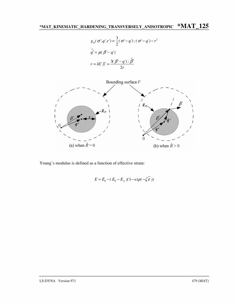
*MAT_KINEMATIC_HARDENING_TRANSVERSELY_ANISOTROPIC *MAT_125
LS-DYNA Version 971 479 (MAT)
23
2
3
2
o
o
g ( ',q',r') ( ' q') : ( ' q') r
q ( ' q')
( ' q') :r h ,
r
σ σ σ σ
μ β
β β
= − − −
′ = −
′−= Γ Γ =
Young’s modulus is defined as a function of effective strain:
0 0 1AE E ( E E )( exp( ))ζ ε= − − − −

*MAT_126 *MAT_MODIFIED_HONEYCOMB
480 (MAT) LS-DYNA Version 971
*MAT_MODIFIED_HONEYCOMB
This is Material Type 126. The major use of this material model is for aluminum honeycomb crushable foam materials with anisotropic behavior. Three yield surfaces are available. In the first, nonlinear elastoplastic material behavior can be defined separately for all normal and shear stresses, which are considered to be fully uncoupled. In the second, a yield surface is defined that considers the effects of off-axis loading. The second yield surface is transversely anisotropic. A drawback of this second yield surface is that the material can collapse in a shear mode due to low shear resistance. There was no obvious way of increasing the shear resistance without changing the behavior in purely uniaxial compression. Therefore, in the third option, the model has been modified so that the user can prescribe the shear and hydrostatic resistance in the material without affecting the uniaxial behavior. The choice of the second yield surface is flagged by the sign of the first load curve ID, LCA. The third yield surface is flagged by the sign of ECCU, which becomes the initial stress yield limit in simple shear. A description is given below.
The development of the second and third yield surfaces are based on experimental test results of aluminum honeycomb specimens at Toyota Motor Corporation.
The default element for this material is solid type 0, a nonlinear spring type brick element. The recommended hourglass control is the type 2 viscous formulation for one point integrated solid elements. The stiffness form of the hourglass control when used with this constitutive model can lead to nonphysical results since strain localization in the shear modes can be inhibited.
Card 1 1 2 3 4 5 6 7 8
Variable MID RO E PR SIGY VF MU BULK
Type A8 F F F F F F F
Default none None None none none none .05 0.0
Card 2
Variable LCA LCB LCC LCS LCAB LCBC LCCA LCSR
Type F F F F F F F F
Default none LCA LCA LCA LCS LCS LCS optional

*MAT_MODIFIED_HONEYCOMB *MAT_126
LS-DYNA Version 971 481 (MAT)
Card 3 1 2 3 4 5 6 7 8
Variable EAAU EBBU ECCU GABU GBCU GCAU AOPT MACF
Type F F F F F F I
Card 4
Variable XP YP ZP A1 A2 A3
Type F F F F F F
Card 5
Variable D1 D2 D3 TSEF SSEF VREF TREF SHDFLG
Type F F F F F F F F
VARIABLE DESCRIPTION
MID Material identification. A unique number or label not exceeding 8 characters must be specified.
RO Mass density.
E Young’s modulus for compacted honeycomb material.
PR Poisson’s ratio for compacted honeycomb material.
SIGY Yield stress for fully compacted honeycomb.
VF Relative volume at which the honeycomb is fully compacted. This parameter is ignored for corotational solid elements, types 0 and 9.
MU μ, material viscosity coefficient. (default=.05) Recommended.
BULK Bulk viscosity flag: EQ.0.0: bulk viscosity is not used. This is recommended. EQ.1.0: bulk viscosity is active and μ=0
This will give results identical to previous versions of LS-DYNA.

*MAT_126 *MAT_MODIFIED_HONEYCOMB
482 (MAT) LS-DYNA Version 971
VARIABLE DESCRIPTION
LCA Load curve ID, see *DEFINE_CURVE: LCA.LT.0: Yield stress as a function of the angle off the material
axis in degrees. LCA.GT.0: sigma-aa versus normal strain component aa. For the
corotational solid elements, types 0 and 9, engineering strain is expected, but for all other solid element formulations a logarithmic strain is expected. See Remarks.
LCB Load curve ID, see *DEFINE_CURVE: LCA.LT.0: strong axis hardening stress as a function of the
volumetric strain. LCA.GT.0: sigma-bb versus normal strain component bb. For the
corotational solid elements, types 0 and 9, engineering strain is expected, but for all other solid element formulations a logarithmic strain is expected. Default LCB=LCA. See Remarks.
LCC Load curve ID, see *DEFINE_CURVE: LCA.LT.0: weak axis hardening stress as a function of the
volumetric strain. LCA.GT.0: sigma-cc versus normal strain component cc. For the
corotational solid elements, types 0 and 9, engineering strain is expected, but for all other solid element formulations a logarithmic strain is expected. Default LCC=LCA. See Remarks.
LCS Load curve ID, see *DEFINE_CURVE: LCA.LT.0: damage curve giving shear stress multiplier as a
function of the shear strain component. This curve definition is optional and may be used if damage is desired. IF SHDFLG=0 (the default), the damage value multiplies the stress every time step and the stress is updated incrementally. The damage curve should be set to unity until failure begins. After failure the value should drop to 0.999 or 0.99 or any number between zero and one depending on how many steps are needed to zero the stress. Alternatively, if SHDFLG=1, the damage value is treated as a factor that scales the shear stress compared to the undamaged value.
LCA.GT.0: shear stress versus shear strain. For the corotational solid elements, types 0 and 9, engineering strain is expected, but for all other solid element formulations a shear strain based on the deformed configuration is used. Default LCS=LCA. Each component of shear stress may have its own load curve. See Remarks.
LCAB Load curve ID, see *DEFINE_CURVE. Default LCAB=LCS: LCA.LT.0: damage curve giving shear ab-stress multiplier as a
function of the ab-shear strain component. This curve definition is optional and may be used if damage is desired. See LCS above.

*MAT_MODIFIED_HONEYCOMB *MAT_126
LS-DYNA Version 971 483 (MAT)
VARIABLE DESCRIPTION
LCA.GT.0: sigma-ab versus shear strain-ab. For the corotational solid elements, types 0 and 9, engineering strain is expected, but for all other solid element formulations a shear strain based on the deformed configuration is used. See Remarks.
LCBC Load curve ID, see *DEFINE_CURVE. Default LCBC=LCS: LCA.LT.0: damage curve giving bc-shear stress multiplier as a
function of the ab-shear strain component. This curve definition is optional and may be used if damage is desired. See LCS above.
LCA.GT.0: sigma-bc versus shear strain-bc. For the corotational solid elements, types 0 and 9, engineering strain is expected, but for all other solid element formulations a shear strain based on the deformed configuration is used. See Remarks.
LCCA Load curve ID, see *DEFINE_CURVE. Default LCCA=LCS: LCA.LT.0: damage curve giving ca-shear stress multiplier as a
function of the ca-shear strain component. This curve definition is optional and may be used if damage is desired. See LCS above.
LCA.GT.0: sigma-ca versus shear strain-ca. For the corotational solid elements, types 0 and 9, engineering strain is expected, but for all other solid element formulations a shear strain based on the deformed configuration is used. See Remarks.
LCSR Load curve ID, see *DEFINE_CURVE, for strain-rate effects defining
the scale factor versus effective strain rate 2
( )3 ij ijε ε ε′ ′= . This is
optional. The curves defined above are scaled using this curve.
EAAU Elastic modulus Eaau in uncompressed configuration.
EBBU Elastic modulus Ebbu in uncompressed configuration.
ECCU Elastic modulus Eccu in uncompressed configuration.
LT.0.0: Ydσ , |ECCU| initial stress limit (yield) in simple shear.
Also, LCA<0 to activate the transversely isotropic yield surface.
GABU Shear modulus Gabu in uncompressed configuration.
GBCU Shear modulus Gbcu in uncompressed configuration.
GCAU Shear modulus Gcau in uncompressed configuration. ECCU.LT.0.0: Y
pσ , GCAU initial stress limit (yield) in hydrostatic
compression. Also, LCA<0 to activate the transversely isotropic yield surface.

*MAT_126 *MAT_MODIFIED_HONEYCOMB
484 (MAT) LS-DYNA Version 971
VARIABLE DESCRIPTION
AOPT Material axes option (see MAT_OPTION TROPIC_ELASTIC for a more complete description):
EQ.0.0: locally orthotropic with material axes determined by element nodes 1, 2, and 4, as with *DEFINE_COORDINATE_ NODES.
EQ.1.0: locally orthotropic with material axes determined by a point in space and the global location of the element center; this is the a-direction.
EQ.2.0: globally orthotropic with material axes determined by vectors defined below, as with *DEFINE_COORDINATE_ VECTOR.
LT.0.0: the absolute value of AOPT is a coordinate system ID number (CID on *DEFINE_COORDINATE_NODES, *DEFINE_ COORDINATE_SYSTEM or *DEFINE_COORDINATE_ VECTOR). Available starting with the R3 release of Version 971.
MACF Material axes change flag: EQ.1: No change, default, EQ.2: switch material axes a and b, EQ.3: switch material axes a and c, EQ.4: switch material axes b and c.
XP YP ZP Coordinates of point p for AOPT = 1.
A1 A2 A3 Components of vector a for AOPT = 2.
D1 D2 D3 Components of vector d for AOPT = 2.
TSEF Tensile strain at element failure (element will erode).
SSEF Shear strain at element failure (element will erode).
VREF This is an optional input parameter for solid elements types 1, 2, 3, 4, and 10. Relative volume at which the reference geometry is stored. At this time the element behaves like a nonlinear spring. The TREF, below, is reached first then VREF will have no effect.
TREF This is an optional input parameter for solid elements types 1, 2, 3, 4, and 10. Element time step size at which the reference geometry is stored. When this time step size is reached the element behaves like a nonlinear spring. If VREF, above, is reached first then TREF will have no effect.
SHDFLG Flag defining treatment of damage from curves LCS, LCAB, LCBC and LCCA (relevant only when LCA < 0):
EQ.0.0: Damage reduces shear stress every time step, EQ.1.0: Damage = (shear stress)/(undamaged shear stress)

*MAT_MODIFIED_HONEYCOMB *MAT_126
LS-DYNA Version 971 485 (MAT)
Remarks:
For efficiency it is strongly recommended that the load curve ID’s: LCA, LCB, LCC, LCS, LCAB, LCBC, and LCCA, contain exactly the same number of points with corresponding strain values on the abscissa. If this recommendation is followed the cost of the table lookup is insignificant. Conversely, the cost increases significantly if the abscissa strain values are not consistent between load curves.
For solid element formulations 1 and 2, the behavior before compaction is orthotropic where the components of the stress tensor are uncoupled, i.e., an a component of strain will generate resistance in the local a-direction with no coupling to the local b and c directions. The elastic moduli vary from their initial values to the fully compacted values linearly with the relative volume:
( )
( )
( )
aa aau aau
bb bbu bbu
cc ccu ccu
E E E E
E E E E
E E E E
β
β
β
= + −
= + −
= + −
( )
( )
( )
ab abu abu
bc bcu bcu
ca cau cau
G E G G
G G G G
G G G G
β
β
β
= + −
= + −
= + −
where
( )11max min ,1 ,0
f
VVβ −
−=
and G is the elastic shear modulus for the fully compacted honeycomb material
( )2 1
EG
v=
+
The relative volume, V, is defined as the ratio of the current volume over the initial volume, and typically, V=1 at the beginning of a calculation.
For corotational solid elements, types 0 and 9, the components of the stress tensor remain uncoupled and the uncompressed elastic moduli are used, that is, the fully compacted elastic moduli are ignored.
The load curves define the magnitude of the stress as the material undergoes deformation. The first value in the curve should be less than or equal to zero corresponding to tension and increase to full compaction. Care should be taken when defining the curves so the extrapolated values do not lead to negative yield stresses.
At the beginning of the stress update we transform each element’s stresses and strain rates into the local element coordinate system. For the uncompacted material, the trial stress components are updated using the elastic interpolated moduli according to:

*MAT_126 *MAT_MODIFIED_HONEYCOMB
486 (MAT) LS-DYNA Version 971
1
1
1
trial
trial
trial
n naa aa aa aa
n nbb bb bb bb
n ncc cc cc cc
E
E
E
σ σ ε
σ σ ε
σ σ ε
+
+
+
= + Δ
= + Δ
= + Δ
1
1
1
2
2
2
trial
trial
trial
n nab ab ab ab
n nbc bc bc bc
n nca ca ca ca
G
G
G
σ σ ε
σ σ ε
σ σ ε
+
+
+
= + Δ
= + Δ
= + Δ
If LCA>0, each component of the updated stress tensor is checked to ensure that it does not exceed the permissible value determined from the load curves, e.g., if
( )1trialnij ij ijσ λσ ε+ >
then
( )1
1
1
trial
trial
nijn
ij ij ij nij
λσσ σ ε
σ
++
+=
On Card 3 ( )ij ijσ ε is defined in the load curve specified in columns 31-40 for the aa stress
component, 41-50 for the bb component, 51-60 for the cc component, and 61-70 for the ab, bc, cb shear stress components. The parameter λ is either unity or a value taken from the load curve number, LCSR, that defines λ as a function of strain-rate. Strain-rate is defined here as the Euclidean norm of the deviatoric strain-rate tensor.
If LCA<0, a transversely isotropic yield surface is obtained where the uniaxial limit
stress, ( ),y volσ ϕ ε , can be defined as a function of angle ϕ with the strong axis and volumetric
strain, volε . In order to facilitate the input of data to such a limit stress surface, the limit stress is written as:
( ) ( ) ( ) ( ) ( ) ( )2 2, cos siny vol b s vol w volσ ϕ ε σ ϕ ϕ σ ε ϕ σ ε= + +
where the functions bσ , sσ , and wσ are represented by load curves LCA, LCB, LCC, respectively. The latter two curves can be used to include the stiffening effects that are observed as the foam material crushes to the point where it begins to lock up. To ensure that the limit stress decreases with respect to the off-angle the curves should be defined such that following equations hold:
( )0
bσ ϕϕ
∂≤
∂and
( ) ( ) 0s vol w volσ ε σ ε− ≥ .
A drawback of this implementation was that the material often collapsed in shear mode due to low shear resistance. There was no way of increasing the shear resistance without changing the behavior in pure uniaxial compression. We have therefore modified the model so that the user can optionally prescribe the shear and hydrostatic resistance in the material without affecting the

*MAT_MODIFIED_HONEYCOMB *MAT_126
LS-DYNA Version 971 487 (MAT)
uniaxial behavior. We introduce the parameters )( volεσ Yp and )( volεσ Y
d as the hydrostatic and
shear limit stresses, respectively. These are functions of the volumetric strain and are assumed given by
vol vol
vol vol
Y Y sp p
Y Y sd d
( ) ( )
( ) ( )
σ ε σ σ ε
σ ε σ σ ε
= +
= +,
where we have reused the densification function sσ . The new parameters are the initial hydrostatic and shear limit stress values, Y
pσ and Ydσ , and are provided by the user as GCAU
and |ECCU|, respectively. The negative sign of ECCU flags the third yield surface option whenever LCA<0. The effect of the third formulation is that (i) for a uniaxial stress the stress limit is given by ),( volεϕσ Y , (ii) for a pressure the stress limit is given by )( volεσ Y
p and (iii) for
a simple shear the stress limit is given by )( volεσ Yd . Experiments have shown that the model
may give noisy responses and inhomogeneous deformation modes if parameters are not chosen with care. We therefore recommend to (i) avoid large slopes in the function Pσ , (ii) let the functions sσ and wσ be slightly increasing and (iii) avoid large differences between the stress limit values voly ( , )σ ϕ ε , )( volεσ Y
p and )( volεσ Yd . These guidelines are likely to contradict how
one would interpret test data and it is up to the user to find a reasonable trade-off between matching experimental results and avoiding the mentioned numerical side effects.
For fully compacted material (element formulations 1 and 2), we assume that the material behavior is elastic-perfectly plastic and updated the stress components according to:
12
2n
trial n devij ij ijs s G ε
+
= + Δ
where the deviatoric strain increment is defined as
13
devij ij kk ijε ε ε δΔ = Δ − Δ
We now check to see if the yield stress for the fully compacted material is exceeded by comparing
( ) 123
2trial trial trialeff ij ijs s s=
the effective trial stress to the yield stress, σy (Card 3, field 21-30). If the effective trial stress exceeds the yield stress we simply scale back the stress components to the yield surface
1 yn trialij ijtrial
eff
s ss
σ+ =
We can now update the pressure using the elastic bulk modulus, K

*MAT_126 *MAT_MODIFIED_HONEYCOMB
488 (MAT) LS-DYNA Version 971
121 nn n
kkp p K ε ++ = − Δ
( )3 1 2
EK
v=
−
and obtain the final value for the Cauchy stress
1 1 1n n nij ij ijs pσ δ+ + += −
After completing the stress update we transform the stresses back to the global configuration.
Figure 126.1. Stress quantity versus strain. Note that the “yield stress” at a strain of zero is nonzero. In the load curve definition the “time” value is the directional strain and the “function” value is the yield stress. Note that for element types 0 and 9 engineering strains are used, but for all other element types the rates are integrated in time.

*MAT_ARRUDA_BOYCE_RUBBER *MAT_127
LS-DYNA Version 971 489 (MAT)
*MAT_ARRUDA_BOYCE_RUBBER
This is Material Type 127. This material model provides a hyperelastic rubber model, see [Arruda and Boyce 1993] combined optionally with linear viscoelasticity as outlined by [Christensen 1980].
Card 1 1 2 3 4 5 6 7 8
Variable MID RO K G N
Type A8 F F F I
Card 2
Variable LCID TRAMP NT
Type F F F
Card Format for Viscoelastic Constants. Up to 6 cards may be input. A keyword card (with a “*” in column 1) terminates this input if less than 6 cards are used.
Optional Cards
1 2 3 4 5 6 7 8
Variable GI BETAI
Type F F
VARIABLE DESCRIPTION
MID Material identification. A unique number or label not exceeding 8 characters must be specified.
RO Mass density
K Bulk modulus
G Shear modulus
N Number of statistical links

*MAT_127 *MAT_ARRUDA_BOYCE_RUBBER
490 (MAT) LS-DYNA Version 971
VARIABLE DESCRIPTION
LCID Optional load curve ID of relaxation curve If constants βι are determined via a least squares fit. This
relaxation curve is shown in Figure 76.1. This model ignores the constant stress.
TRAMP Optional ramp time for loading.
NT Number of Prony series terms in optional fit. If zero, the default is 6. Currently, the maximum number is 6. Values less than 6, possibly 3-5 are recommended, since each term used adds significantly to the cost. Caution should be exercised when taking the results from the fit. Always check the results of the fit in the output file. Preferably, all generated coefficients should be positive. Negative values may lead to unstable results. Once a satisfactory fit has been achieved it is recommended that the coefficients which are written into the output file be input in future runs.
GI Optional shear relaxation modulus for the ith term
BETAI Optional decay constant if ith term
Remarks:
Rubber is generally considered to be fully incompressible since the bulk modulus greatly exceeds the shear modulus in magnitude. To model the rubber as an unconstrained material a hydrostatic work term, ( )HW J , is included in the strain energy functional which is function of
the relative volume, J, [Ogden 1984]:
( ) ( ) ( ) ( )( ) ( ) ( )
2
3 4
2 31 1 111 2 1 1 12 20 1050
4 519 5191 17000 673750
, , 3 9 27
81 243
N N
HN N
W J J J nk J J J
nk J J W J
θ
θ
= − + − + −
+ − + − +
where the hydrostatic work term is in terms of the bulk modulus, K, and the third invariant, J, as:
( ) ( )21
2H
KW J J= −
Rate effects are taken into account through linear viscoelasticity by a convolution integral of the form:
( )0
tkl
ij ijklg t dεσ τ ττ
∂= −∂
or in terms of the second Piola-Kirchhoff stress, ijS , and Green's strain tensor, ijE ,

*MAT_ARRUDA_BOYCE_RUBBER *MAT_127
LS-DYNA Version 971 491 (MAT)
( )0
tkl
ij ijkl
ES G t dτ τ
τ∂= −∂
where ( )ijklg t τ− and ( )ijklG t τ− are the relaxation functions for the different stress measures.
This stress is added to the stress tensor determined from the strain energy functional.
If we wish to include only simple rate effects, the relaxation function is represented by six terms from the Prony series:
( ) 01
Nt
mm
g t e βα α −
== +
given by,
( )1
i
nt
ii
g t G e β−
==
This model is effectively a Maxwell fluid which consists of a dampers and springs in series. We characterize this in the input by shear moduli, Gi , and decay constants, βi . The viscoelastic behavior is optional and an arbitrary number of terms may be used.

*MAT_128 *MAT_HEART_TISSUE
492 (MAT) LS-DYNA Version 971
*MAT_HEART_TISSUE
This is Material Type 128. This material model provides a heart tissue model described in the paper by Guccione, McCulloch, and Waldman [1991]. This model is transversely isotropic.
Card 1 1 2 3 4 5 6 7 8
Variable MID RO C B1 B2 B3 P
Type A8 F F F F F F
Card 2
Variable AOPT MACF
Type F I
Card 3
Variable XP YP ZP A1 A2 A3
Type F F F F F F
Card 4
Variable V1 V2 V3 D1 D2 D3 BETA
Type F F F F F F F
VARIABLE DESCRIPTION
MID Material identification. A unique number or label not exceeding 8 characters must be specified.
RO Mass density
C Material coefficient.

*MAT_HEART_TISSUE *MAT_128
LS-DYNA Version 971 493 (MAT)
VARIABLE DESCRIPTION
B1 b1 ,material coefficient.
B2 b2 ,material coefficient.
B3 b3 ,material coefficient.
P Pressure in the muscle tissue.
AOPT Material axes option (see MAT_OPTION TROPIC_ELASTIC for a more complete description):
EQ.0.0: locally orthotropic with material axes determined by element nodes 1, 2, and 4, as with *DEFINE_COORDINATE_ NODES.
EQ.1.0: locally orthotropic with material axes determined by a point in space and the global location of the element center; this is the a-direction.
EQ.2.0: globally orthotropic with material axes determined by vectors defined below, as with *DEFINE_COORDINATE_ VECTOR.
EQ.3.0: locally orthotropic material axes determined by rotating the material axes about the element normal by an angle, BETA, from a line in the plane of the element defined by the cross product of the vector v with the element normal.
EQ.4.0: locally orthotropic in cylindrical coordinate system with the material axes determined by a vector v, and an originating point, P, which define the centerline axis.
LT.0.0: the absolute value of AOPT is a coordinate system ID number (CID on *DEFINE_COORDINATE_NODES, *DEFINE_ COORDINATE_SYSTEM or *DEFINE_COORDINATE_ VECTOR). Available in R3 version of 971 and later.
MACF Material axes change flag for brick elements: EQ.1: No change, default, EQ.2: switch material axes a and b, EQ.3: switch material axes a and c, EQ.4: switch material axes b and c.
XP,YP,ZP xp yp zp, define coordinates of point p for AOPT = 1 and 4.
A1,A2,A3 a1 a2 a3, define components of vector a for AOPT = 2.
D1,D2,D3 d1 d2 d3, define components of vector d for AOPT = 2.
V1,V2,V3 v1 v2 v3, define components of vector v for AOPT = 3 and 4.
BETA Material angle in degrees for AOPT = 3, may be overridden on the element card, see *ELEMENT_SOLID_ORTHO.
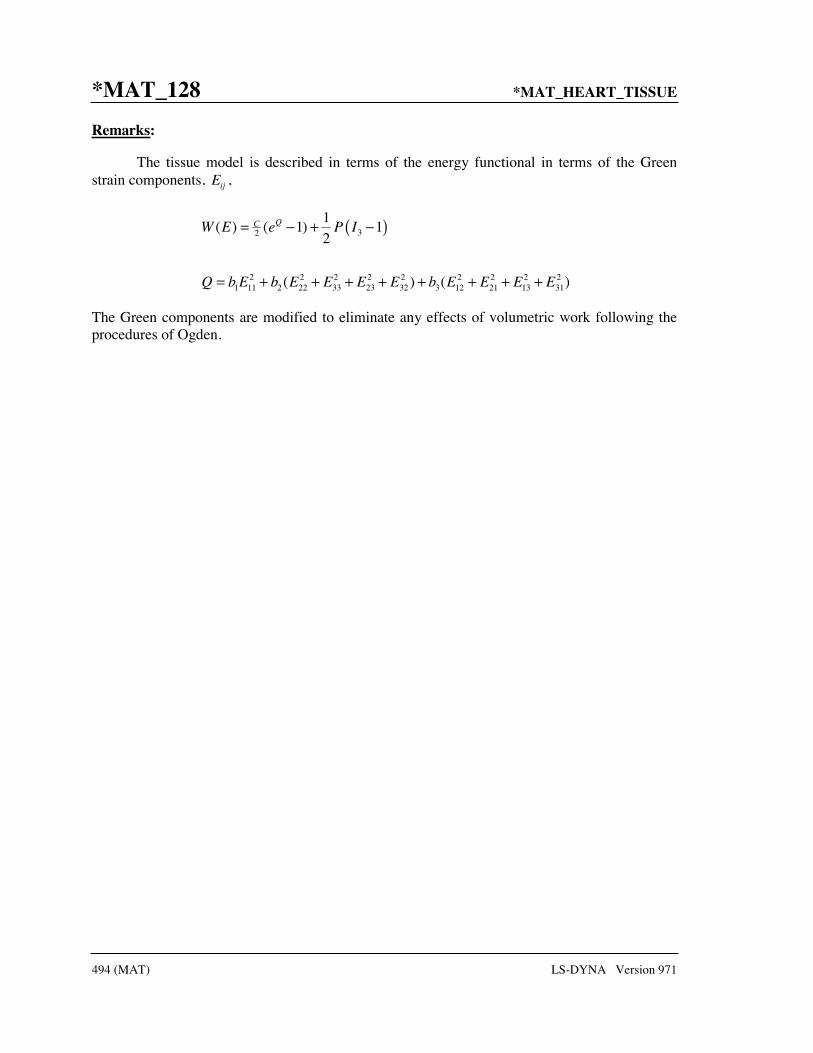
*MAT_128 *MAT_HEART_TISSUE
494 (MAT) LS-DYNA Version 971
Remarks:
The tissue model is described in terms of the energy functional in terms of the Green strain components, Eij ,
( )32
2 2 2 2 2 2 2 2 21 11 2 22 33 23 32 3 12 21 13 31
1( ) ( 1) 1
2
( ) ( )
QCW E e P I
Q b E b E E E E b E E E E
= − + −
= + + + + + + + +
The Green components are modified to eliminate any effects of volumetric work following the procedures of Ogden.

*MAT_LUNG_TISSUE *MAT_129
LS-DYNA Version 971 495 (MAT)
*MAT_LUNG_TISSUE
This is Material Type 129. This material model provides a hyperelastic model for heart tissue, see [Vawter 1980] combined optionally with linear viscoelasticity as outlined by [Christensen 1980].
Card 1 1 2 3 4 5 6 7 8
Variable MID RO K C DELTA ALPHA BETA
Type A8 F F F I
Card 2
Variable C1 C2 LCID TRAMP NT
Type F F F F F
Card Format for Viscoelastic Constants. Up to 6 cards may be input. A keyword card (with a “*” in column 1) terminates this input if less than 6 cards are used.
Optional Cards
1 2 3 4 5 6 7 8
Variable GI BETAI
Type F F
VARIABLE DESCRIPTION
MID Material identification. A unique number or label not exceeding 8 characters must be specified.
RO Mass density
K Bulk modulus
C Material coefficient.
DELTA Δ , material coefficient.

*MAT_129 *MAT_LUNG_TISSUE
496 (MAT) LS-DYNA Version 971
VARIABLE DESCRIPTION
ALPHA α , material coefficient.
BETA β , material coefficient.
C1 Material coefficient.
C2 Material coefficient.
LCID Optional load curve ID of relaxation curve If constants βι are determined via a least squares fit. This
relaxation curve is shown in Figure 76.1. This model ignores the constant stress.
TRAMP Optional ramp time for loading.
NT Number of Prony series terms in optional fit. If zero, the default is 6. Currently, the maximum number is 6. Values less than 6, possibly 3-5 are recommended, since each term used adds significantly to the cost. Caution should be exercised when taking the results from the fit. Always check the results of the fit in the output file. Preferably, all generated coefficients should be positive. Negative values may lead to unstable results. Once a satisfactory fit has been achieved it is recommended that the coefficients which are written into the output file be input in future runs.
GI Optional shear relaxation modulus for the ith term
BETAI Optional decay constant if ith term
Remarks:
The material is described by a strain energy functional expressed in terms of the invariants of the Green Strain:
( )
21 2 2( ) (1 )1
1 22
2 41 23
12( , ) 1
2 (1 )
1
I I CC CW I I e A
C
A I I
α β+ += + −Δ Δ +
= + −
where the hydrostatic work term is in terms of the bulk modulus, K, and the third invariant, J, as:
( ) 2( 1)2H
KW J J= −
Rate effects are taken into account through linear viscoelasticity by a convolution integral of the form:

*MAT_LUNG_TISSUE *MAT_129
LS-DYNA Version 971 497 (MAT)
( )0
tkl
ij ijklg t d∂εσ τ τ∂τ
= −
or in terms of the second Piola-Kirchhoff stress, Sij , and Green's strain tensor, Eij ,
( )0
tkl
ij ijkl
ES G t d
∂τ τ∂τ
= −
where gijkl(t − τ ) and Gijkl t − τ( ) are the relaxation functions for the different stress measures.
This stress is added to the stress tensor determined from the strain energy functional.
If we wish to include only simple rate effects, the relaxation function is represented by six terms from the Prony series:
01
( )N
tm
m
g t e βα α −
== +
given by,
1
( ) i
nt
ii
g t G e β−
==
This model is effectively a Maxwell fluid which consists of a dampers and springs in series. We characterize this in the input by shear moduli, Gi , and decay constants, βi . The viscoelastic behavior is optional and an arbitrary number of terms may be used.
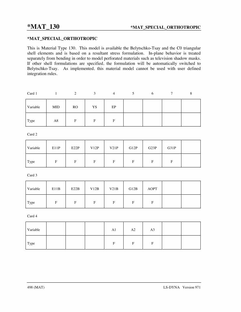
*MAT_130 *MAT_SPECIAL_ORTHOTROPIC
498 (MAT) LS-DYNA Version 971
*MAT_SPECIAL_ORTHOTROPIC
This is Material Type 130. This model is available the Belytschko-Tsay and the C0 triangular shell elements and is based on a resultant stress formulation. In-plane behavior is treated separately from bending in order to model perforated materials such as television shadow masks. If other shell formulations are specified, the formulation will be automatically switched to Belytschko-Tsay. As implemented, this material model cannot be used with user defined integration rules.
Card 1 1 2 3 4 5 6 7 8
Variable MID RO YS EP
Type A8 F F F
Card 2
Variable E11P E22P V12P V21P G12P G23P G31P
Type F F F F F F F
Card 3
Variable E11B E22B V12B V21B G12B AOPT
Type F F F F F F
Card 4
Variable A1 A2 A3
Type F F F

*MAT_SPECIAL_ORTHOTROPIC *MAT_130
LS-DYNA Version 971 499 (MAT)
Card 5 1 2 3 4 5 6 7 8
Variable V1 V2 V3 D1 D2 D3 BETA
Type F F F F F F F
VARIABLE DESCRIPTION
MID Material identification. A unique number or label not exceeding 8 characters must be specified.
RO Mass density.
YS Yield stress. This parameter is optional and is approximates the yield condition. Set to zero if the behavior is elastic.
EP Plastic hardening modulus.
E11P E11p, for in plane behavior.
E22P E22p, for in plane behavior.
V12P ν12p, for in plane behavior.
V11P ν21p, for in plane behavior.
G12P G12p, for in plane behavior.
G23P G23p, for in plane behavior.
G31P G31p, for in plane behavior.
E11B E11b, for bending behavior.
E22B E22b, for bending behavior.
V12B ν12b, for bending behavior.
V21B ν21b, for bending behavior.
G12B G12b, for bending behavior.

*MAT_130 *MAT_SPECIAL_ORTHOTROPIC
500 (MAT) LS-DYNA Version 971
VARIABLE DESCRIPTION
AOPT Material axes option (see MAT_OPTION TROPIC_ELASTIC for a more complete description):
EQ.0.0: locally orthotropic with material axes determined by element nodes 1, 2, and 4, as with *DEFINE_COORDINATE_ NODES.
EQ.2.0: globally orthotropic with material axes determined by vectors defined below, as with *DEFINE_COORDINATE_ VECTOR.
EQ.3.0: locally orthotropic material axes determined by rotating the material axes about the element normal by an angle, BETA, from a line in the plane of the element defined by the cross product of the vector v with the element normal.
LT.0.0: the absolute value of AOPT is a coordinate system ID number (CID on *DEFINE_COORDINATE_NODES, *DEFINE_ COORDINATE_SYSTEM or *DEFINE_COORDINATE_ VECTOR). Available in R3 version of 971 and later.
A1,A2,A3 a1 a2 a3, define components of vector a for AOPT = 2.
D1,D2,D3 d1 d2 d3, define components of vector d for AOPT = 2.
V1,V2,V3 v1 v2 v3, define components of vector v for AOPT = 3.
BETA Material angle in degrees for AOPT = 3, may be overridden on the element card, see *ELEMENT_SHELL_BETA.
Remarks:
The in-plane elastic matrix for in-plane, plane stress behavior is given by:
11 12
12 22
44
55
66
0 0 0
0 0 0
0 0 0 0
0 0 0 0
0 0 0 0
p p
p p
in plane p
p
p
Q Q
Q Q
C Q
Q
Q
=
The terms Qijp are defined as:

*MAT_SPECIAL_ORTHOTROPIC *MAT_130
LS-DYNA Version 971 501 (MAT)
1111
12 21
2222
12 21
12 1112
12 21
44 12
55 23
66 31
1
1
1
pp
p p
pp
p p
p pp
p p
p p
p p
p p
EQ
EQ
EQ
Q G
Q G
Q G
ν ν
ν νν
ν ν
=−
=−
=−
=
=
=
The elastic matrix for bending behavior is given by:
11 12
12 22
44
0
0
0 0
b b
bending b b
b
Q Q
C Q Q
Q
=
The terms Qijp are similarly defined.

*MAT_131 *MAT_ISOTROPIC_SMEARED_CRACK
502 (MAT) LS-DYNA Version 971
*MAT_ISOTROPIC_SMEARED_CRACK
This is Material Type 131. This model was developed by Lemmen and Meijer [2001] as a smeared crack model for isotropic materials. This model is available of solid elements only and is restricted to cracks in the x-y plane. Users should choose other models unless they have the report by Lemmen and Meijer [2001].
Card 1 1 2 3 4 5 6 7 8
Variable MID RO E PR ISPL SIGF GK SR
Type A8 F F F I F F F
VARIABLE DESCRIPTION
MID Material identification. A unique number or label not exceeding 8 characters must be specified.
RO Mass density
E Young’s modulus
PR Poisson’s ratio
ISPL Failure option: EQ.0: Maximum principal stress criterion EQ.5: Smeared crack model EQ.6: Damage model based on modified von Mises strain.
GK Critical energy release rate.
SR Strength ratio.
Remarks:
The following documentation is taken nearly verbatim from the documentation of Lemmen and Meijer [2001].
Three methods are offered to model progressive failure. The maximum principal stress criterion detects failure if the maximum (most tensile) principal stress exceeds maxσ . Upon
failure, the material can no longer carry stress.
The second failure model is the smeared crack model with linear softening stress-strain using equivalent uniaxial strains. Failure is assumed to be perpendicular to the principal strain directions. A rotational crack concept is employed in which the crack directions are related to

*MAT_ISOTROPIC_SMEARED_CRACK *MAT_131
LS-DYNA Version 971 503 (MAT)
the current directions of principal strain. Therefore crack directions may rotate in time. Principal stresses are expressed as
1 11 11
2 2 2 2 2
33 3 3 3
EE 0 0
0 E 0 E
0 0 E E
εσ εσ ε εσ ε ε
= = (131.1)
with 1E , 2E and 3E secant stiffness in the terms that depend on internal variables.
In the model developed for DYCOSS it has been assumed that there is no interaction between the three directions in which case stresses simply follow from
,
,, ,
, ,
,
E 0
( ) 1
0
j j j ini
j j inij j j ini j j ult
j ult j ini
j j ult
if
if
if
ε ε ε
ε εσ ε σ ε ε ε
ε εε ε
≤ ≤
−= − < ≤
−
>
(131.2)
with σ the ultimate stress, ,j iniε the damage threshold, and ,j ultε the ultimate strain in j-direction.
The damage threshold is defined as
, Ej ini
σε = (131.3)
The ultimate strain is obtained by relating the crack growth energy and the dissipated energy
,j ultd dV GAσ ε = (131.4)
with G the energy release rate, V the element volume and A the area perpendicular to the principal strain direction. The one point elements LS-DYNA have a single integration point and the integral over the volume may be replaced by the volume. For linear softening it follows
,
2j ult
GA
Vε
σ= (131.5)
The above formulation may be regarded as a damage equivalent to the maximum principle stress criterion.
The third model is a damage model represented by Brekelmans et. al [1991]. Here the Cauchy stress tensor σ is expressed as
(1 )EDσ ε= − (131.6)

*MAT_131 *MAT_ISOTROPIC_SMEARED_CRACK
504 (MAT) LS-DYNA Version 971
where D represents the current damage and the factor (1-D) is the reduction factor caused by damage. The scalar damage variable is expressed as function of a so-called damage equivalent strain dε
( )( ) 1
( )
ini ult d
d
d ult ini
D Dε ε εεε ε ε
−= = −−
(131.7)
and
1 1 2
2
2
1 1 1 6
2 (1 2 ) 2 1 2 (1 )d
k k kJ J J
k v k v vε − −= + +
− − + (131.8)
where the constant k represents the ratio of the strength in tension over the strength in compression
,
,
ult tension
ult compression
kσ
σ= (131.9)
J1 resp. J2 are the first and second invariant of the strain tensor representing the volumetric and the deviatoric straining respectively
1
22
( )
1( ) ( )
3
J tr
J tr tr
ε
ε ε ε
=
= ⋅ − (131.10)
If the compression and tension strength are equal the dependency on the volumetric strain vanishes in (8) and failure is shear dominated. If the compressive strength is much larger than the strength in tension, k becomes small and the J1 terms in (131.8) dominate the behavior.

*MAT_ORTHOTROPIC_SMEARED_CRACK *MAT_132
LS-DYNA Version 971 505 (MAT)
*MAT_ORTHOTROPIC_SMEARED_CRACK
This is Material Type 132. This material is a smeared crack model for orthotropic materials.
Card 1 1 2 3 4 5 6 7 8
Variable MID RO EA EB EC PRBA PRCA PRCB
Type A8 F F F F F F F
Card 2
Variable UINS UISS CERRMI CERRMII IND ISD
Type F F F F I I
Card 3
Variable GAB GBC GCA AOPT
Type F F F F
Card 4
Variable XP YP ZP A1 A2 A3 MACF
Type F F F F F F I
Card 5
Variable V1 V2 V3 D1 D2 D3 BETA REF
Type F F F F F F F F

*MAT_132 *MAT_ORTHOTROPIC_SMEARED_CRACK
506 (MAT) LS-DYNA Version 971
VARIABLE DESCRIPTION
MID Material identification. A unique number or label not exceeding 8 characters must be specified.
RO Mass density.
EA Ea, Young’s modulus in a-direction.
EB Eb, Young’s modulus in b-direction.
EC Ec, Young’s modulus in c-direction
PRBA νba, Poisson’s ratio ba.
PRCA νca, Poisson’s ratio ca.
PRCB νcb, Poisson’s ratio cb.
UINS Ultimate interlaminar normal stress.
UISS Ultimate interlaminar shear stress.
CERRMI Critical energy release rate mode I
CERRMII Critical energy release rate mode II
IND Interlaminar normal direction : EQ.1.0: Along local a axis EQ.2.0: Along local b axis EQ.3.0: Along local c axis
ISD Interlaminar shear direction : EQ.4.0: Along local ab axis EQ.5.0: Along local bc axis EQ.6.0: Along local ca axis
GAB Gab, shear modulus ab.
GBC Gbc, shear modulus bc.
GCA Gca, shear modulus ca.
AOPT Material axes option, see Figure 2.1. EQ.0.0: locally orthotropic with material axes determined by element nodes as shown in Figure 2.1. Nodes 1, 2, and 4 of an element are identical to the nodes used for the definition of a coordinate system as by *DEFINE_COORDINATE_NODES.

*MAT_ORTHOTROPIC_SMEARED_CRACK *MAT_132
LS-DYNA Version 971 507 (MAT)
VARIABLE DESCRIPTION
EQ.1.0: locally orthotropic with material axes determined by a point in space and the global location of the element center; this is the a-direction. This option is for solid elements only.
EQ.2.0: globally orthotropic with material axes determined by vectors defined below, as with *DEFINE_COORDINATE_ VECTOR.
EQ.3.0: locally orthotropic material axes determined by rotating the material axes about the element normal by an angle, BETA, from a line in the plane of the element defined by the cross product of the vector v with the element normal. The plane of a solid element is the midsurface between the inner surface and outer surface defined by the first four nodes and the last four nodes of the connectivity of the element, respectively.
EQ.4.0: locally orthotropic in cylindrical coordinate system with the material axes determined by a vector v, and an originating point, P, which define the centerline axis. This option is for solid elements only.
LT.0.0: the absolute value of AOPT is a coordinate system ID number (CID on *DEFINE_COORDINATE_NODES, *DEFINE_ COORDINATE_SYSTEM or *DEFINE_COORDINATE_ VECTOR). Available in R3 version of 971 and later.
XP YP ZP Define coordinates of point p for AOPT = 1 and 4.
A1 A2 A3 Define components of vector a for AOPT = 2.
MACF Material axes change flag for brick elements: EQ.1: No change, default,
EQ.2: switch material axes a and b, EQ.3: switch material axes a and c, EQ.4: switch material axes b and c.
V1 V2 V3 Define components of vector v for AOPT = 3 and 4.
D1 D2 D3 Define components of vector d for AOPT = 2:
BETA Material angle in degrees for AOPT = 3, may be overridden on the element card, see *ELEMENT_SHELL_BETA or *ELEMENT_ SOLID_ORTHO.
REF Use reference geometry to initialize the stress tensor. The reference geometry is defined by the keyword: *INITIAL_FOAM_ REFERENCE_GEOMETRY (see there for more details).
EQ.0.0: off, EQ.1.0: on.

*MAT_132 *MAT_ORTHOTROPIC_SMEARED_CRACK
508 (MAT) LS-DYNA Version 971
Remarks:
This is an orthotropic material with optional delamination failure for brittle composites. The elastic formulation is identical to the DYNA3D model that uses total strain formulation. The constitutive matrix C that relates to global components of stress to the global components of strain is defined as:
C T C TTL=
where T is the transformation matrix between the local material coordinate system and the global system and CL is the constitutive matrix defined in terms of the material constants of the local
orthogonal material axes a, b, and c (see DYNA3D use manual).
Failure is described using linear softening stress strain curves for interlaminar normal and interlaminar shear direction. The current implementation for failure is essentially 2-D. Damage can occur in interlaminar normal direction and a single interlaminar shear direction. The orientation of these directions w.r.t. the principal material directions have to be specified by the user.
Based on specified values for the ultimate stress and the critical energy release rate bounding surfaces are defined
( )
( )
n n n n
s s s s
f
f
σ σ εσ σ ε
= −= −
where the subscripts n and s refer to the normal and shear component. If stresses exceed the bounding surfaces inelastic straining occurs. The ultimate strain is obtained by relating the crack growth energy and the dissipated energy. For solid elements with a single integration point it can be derived
,
,
2 i
i ult
i ult
GA
Vε
σ=
with iG the critical energy release rate, V the element volume, A the area perpendicular to the active normal direction and ,i ultσ the ultimate stress. For the normal component failure can only occur under tensile loading. For shear component the behavior is symmetric around zero. The resulting stress bounds are depicted in Figure 132.1. Unloading is modeled with a Secant stiffness.

*MAT_ORTHOTROPIC_SMEARED_CRACK *MAT_132
LS-DYNA Version 971 509 (MAT)
Figure 132.1. Shows stress bounds for the active normal component (left) and the archive shear component (right).

*MAT_133 *MAT_BARLAT_YLD2000
510 (MAT) LS-DYNA Version 971
*MAT_BARLAT_YLD2000
This is Material Type 133. This model was developed by Barlat et al. [2003] to overcome some shortcomings of the six parameter Barlat model implemented as material 33 (MAT_ BARLAT_YLD96) in LS-DYNA. This model is available for shell elements only.
Card 1 1 2 3 4 5 6 7 8
Variable MID RO E PR FIT BETA ITER
Type A8 F F F F F F
Card 2
Variable K E0 N C P HARD A
Type F F F F F F F
Define the following card if and only if FIT=0
Card 3 1 2 3 4 5 6 7 8
Variable ALPHA1 ALPHA2 ALPHA3 ALPHA4 ALPHA5 ALPHA6 ALPHA7 ALPHA8
Type F F F F F F F F
Define the following two cards if and only if FIT=1
Card 3 1 2 3 4 5 6 7 8
Variable SIG00 SIG45 SIG90 R00 R45 R90
Type F F F F F F

*MAT_BARLAT_YLD2000 *MAT_133
LS-DYNA Version 971 511 (MAT)
Card 4 1 2 3 4 5 6 7 8
Variable SIGXX SIGYY SIGXY DXX DYY DXY
Type F F F F F F
Card 4/5
Variable AOPT OFFANG
Type F F
Card 5/6
Variable A1 A2 A3
Type F F F
Card 6/7
Variable V1 V2 V3 D1 D2 D3
Type F F F F F F
VARIABLE DESCRIPTION
MID Material identification. A unique number or label not exceeding 8 characters must be specified.
RO Mass density
E Young’s modulus
PR Poisson’s ratio

*MAT_133 *MAT_BARLAT_YLD2000
512 (MAT) LS-DYNA Version 971
VARIABLE DESCRIPTION
FIT Material parameter fit flag: EQ.0.0: Material parameters are used directly on card 3. EQ.1.0: Material parameters are determined from test data on cards 3 and 4.
BETA Hardening parameter. Any value ranging from 0 (isotropic hardening) to 1 (kinematic hardening) may be input.
ITER Plastic iteration flag: EQ.0.0: Plane stress algorithm for stress return
EQ.1.0: Secant iteration algorithm for stress return
ITER provides an option of using three secant iterations for determining the thickness strain increment as experiments have shown that this leads to a more accurate prediction of shell thickness changes for rapid processes. A significant increase in computation time is incurred with this option so it should be used only for applications associated with high rates of loading and/or for implicit analysis.
K Material parameter: HARD.EQ.1.0: k, strength coefficient for exponential hardening
HARD.EQ.2.0: a in Voce hardening law
E0 Material parameter: HARD.EQ.1.0: ε0, strain at yield for exponential hardening
HARD.EQ.2.0: b in Voce hardening law
N Material parameter: HARD.EQ.1.0: n, exponent for exponential hardening
HARD.EQ.2.0: c in Voce hardening law
C Cowper-Symonds strain rate parameter, C, see formula below.
P Cowper-Symonds strain rate parameter, p.
1/
( , ) ( ) 1p
pvy p p y p C
εσ ε ε σ ε= +
HARD Hardening law:
EQ.1.0: Exponential hardening: ( )0σ ε ε= +n
y pk
EQ.2.0: Voce hardening: pc
y a be εσ −= − LT.0.0: Absolute value defines load curve ID
A Flow potential exponent

*MAT_BARLAT_YLD2000 *MAT_133
LS-DYNA Version 971 513 (MAT)
VARIABLE DESCRIPTION
ALPHA1 α1, see equations below
ALPHA2 α2, see equations below
ALPHA3 α3, see equations below
ALPHA4 α4, see equations below
ALPHA5 α5, see equations below
ALPHA6 α6, see equations below
ALPHA7 α7, see equations below
ALPHA8 α8, see equations below
SIG00 Yield stress in 00 direction
SIG45 Yield stress in 45 direction
SIG90 Yield stress in 90 direction
R00 R-value in 00 direction
R45 R-value in 45 direction
R90 R-value in 90 direction
SIGXX xx-component of stress on yield surface (See Remark 2).
SIGYY yy-component of stress on yield surface (See Remark 2).
SIGXY xy-component of stress on yield surface (See Remark 2).
DXX xx-component of tangent to yield surface (See Remark 2).
DYY yy-component of tangent to yield surface (See Remark 2).
DXY xy-component of tangent to yield surface (See Remark 2).
AOPT Material axes option: EQ.0.0: locally orthotropic with material axes determined by
element nodes as shown in Figure 20.1. Nodes 1, 2, and 4 of an element are identical to the nodes used for the definition of a coordinate system as by *DEFINE_COORDINATE_NODES

*MAT_133 *MAT_BARLAT_YLD2000
514 (MAT) LS-DYNA Version 971
VARIABLE DESCRIPTION
EQ.2.0: globally orthotropic with material axes determined by vectors defined below, as with *DEFINE_COORDINATE_ VECTOR
EQ.3.0: locally orthotropic material axes determined by offsetting the material axes by an angle, OFFANG, from a line determined by
taking the cross product of the vector v with the normal to the plane of the element.
LT.0.0: the absolute value of AOPT is a coordinate system ID number (CID on *DEFINE_COORDINATE_NODES, *DEFINE_ COORDINATE_SYSTEM or *DEFINE_COORDINATE_ VECTOR). Available in R3 version of 971 and later.
OFFANG Offset angle for AOPT=3
A1 A2 A3 Components of vector a for AOPT=2
V1 V2 V3 Components of vector v for AOPT=3
D1 D2 D3 Components of vector d for AOPT=2
Remarks:
1. Strain rate is accounted for using the Cowper and Symonds model which scales the yield stress with the factor
1
1p
C
ε+
where ε is the strain rate. A fully viscoplastic formulation is optional which incorporates the Cowper and Symonds formulation within the yield surface. An additional cost is incurred but the improvement allows for dramatic results. To ignore strain rate effects set both SRC and SRP to zero.
2. The yield condition for this material can be written
0),,(
),2,2(),,( eff
≤
−−−−−−=
βεεσ
ασαασαασσε
pptY
xyxyxxyyyyyyxxxxpf
where
aa
a
a
xyyyxx
XXXX
XX
sss
2121
21
/1
eff
''2''''''2''
'''
)'''(2
1),,(
+++=
−=
+=
φ
φ
φφσ
.

*MAT_BARLAT_YLD2000 *MAT_133
LS-DYNA Version 971 515 (MAT)
The iX ' and ''iX are eigenvalues of ijX ' and ijX '' and are given by
( )( )
2 21 11 22 11 22 12
2 22 11 22 11 22 12
1' ' ' ( ' ' ) 4 '
21
' ' ' ( ' ' ) 4 '2
X X X X X X
X X X X X X
= + + − +
= + − − +
and
( )( )2
122
221122112
212
2221122111
''4)''''(''''2
1''
''4)''''(''''2
1''
XXXXXX
XXXXXX
+−−+=
+−++=
respectively. The ijX ' and ijX '' are given by
=
xy
yy
xx
s
s
s
L
LL
LL
X
X
X
33
2221
1211
12
22
11
'00
0''
0''
'
'
'
=
xy
yy
xx
s
s
s
L
LL
LL
X
X
X
33
2221
1211
12
22
11
''00
0''''
0''''
''
''
''
where
−−
=
7
2
1
33
22
21
12
11
300
020
010
001
002
3
1
'
'
'
'
'
ααα
L
L
L
L
L
−−−−−−
−−
=
8
6
5
4
3
33
22
21
12
11
90000
02282
01444
04441
02822
9
1
''
''
''
''
''
ααααα
L
L
L
L
L
The parameters 1α to 8α are the parameters that determines the shape of the yield surface.
The material parameters can be determined from three uniaxial tests and a more general test. From the uniaxial tests the yield stress and R-values are used and from the general test an arbitrary point on the yield surface is used given by the stress components in the material system as
=
xy
yy
xx
σσσ
together with a tangent of the yield surface in that particular point. For the latter the tangential direction should be determined so that
02 =++ pxyxy
pyyyy
pxxxx ddd εεε
The biaxial data can be set to zero in the input deck for LS-DYNA to just fit the uniaxial data.

*MAT_135 *MAT_WTM_STM
516 (MAT) LS-DYNA Version 971
*MAT_WTM_STM
This is material type 135. This anisotropic-viscoplastic material model adopts two yield criteria for metals with orthotropic anisotropy proposed by Barlat and Lian [1989] (Weak Texture Model) and Aretz [2004] (Strong Texture Model).
Card 1 1 2 3 4 5 6 7 8
Variable MID RO E PR NUMFI EPSC WC TAUC
Type A8 F F F F F F F
Card 2
Variable SIGMA0 QR1 CR1 QR2 CR2 K LC FLG
Type F F F F F F F F
Describe the following card for FLG = 0
Card 3 1 2 3 4 5 6 7 8
Variable A1 A2 A3 A4 A5 A6 A7 A8
Type F F F F F F F F
Describe the following card for FLG = 1
Card 3 1 2 3 4 5 6 7 8
Variable S00 S45 S90 SBB R00 R45 R90 RBB
Type F F F F F F F F

*MAT_WTM_STM *MAT_135
LS-DYNA Version 971 517 (MAT)
Describe the following card for FLG = 2
Card 3 1 2 3 4 5 6 7 8
Variable A C H P
Type F F F F
Card 4
Variable QX1 CX1 QX2 CX2 EDOT M EMIN
Type F F F F F F F
Card 5
Variable AOPT BETA
Type F F
Card 6
Variable XP YP ZP A1 A2 A3
Type F F F F F F
Card 7
Variable V1 V2 V3 D1 D2 D3
Type F F F F F F

*MAT_135 *MAT_WTM_STM
518 (MAT) LS-DYNA Version 971
VARIABLE DESCRIPTION
MID Material identification. A unique number or label not exceeding 8 characters must be specified.
RO Mass density
E Young’s modulus
PR Poisson’s ratio
NUMFI Number of through thickness integration points that must fail before the element is deleted (remember to change this number if switching between full and reduced integration type of elements).
EPSC Critical value tCε of the plastic thickness strain (used in the CTS fracture
criterion).
WC Critical value cW for the Cockcroft-Latham fracture criterion
TAUC Critical value cτ for the Bressan-Williams shear fracture criterion
SIGMA0 Initial mean value of yield stress 0σ
QR1 Isotropic hardening parameter 1RQ
CR1 Isotropic hardening parameter 1RC
QR2 Isotropic hardening parameter 2RQ
CR2 Isotropic hardening parameter 2RC
K k equals half YLD2003 exponent m . Recommended value for FCC materials is 8m = , i.e. 4k = .
LC First load curve number for process effects, i.e. the load curve describing the relation between the pre-strain and the yield stress 0σ . Similar curves
for 1RQ , 1RC , 2RQ , 2RC , and cW must follow consecutively from this
number.
A1 Yld2003 parameter 1a
A2 Yld2003 parameter 2a

*MAT_WTM_STM *MAT_135
LS-DYNA Version 971 519 (MAT)
VARIABLE DESCRIPTION
A3 Yld2003 parameter 3a
A4 Yld2003 parameter 4a
A5 Yld2003 parameter 5a
A6 Yld2003 parameter 6a
A7 Yld2003 parameter 7a
A8 Yld2003 parameter 8a
S00 Yield stress in 0° direction
S45 Yield stress in 45° direction
S90 Yield stress in 90° direction
SBB Balanced biaxial flow stress
R00 R-ratio in 0° direction
R45 R-ratio in 45° direction
R90 R-ratio in 90° direction
RBB Balance biaxial flow ratio
A YLD89 parameter a
C YLD89 parameter c
H YLD89 parameter h
P YLD89 parameter p
QX1 Kinematic hardening parameter 1xQ
CX1 Kinematic hardening parameter 1xC
QX2 Kinematic hardening parameter 2xQ

*MAT_135 *MAT_WTM_STM
520 (MAT) LS-DYNA Version 971
VARIABLE DESCRIPTION
CX2 Kinematic hardening parameter 2xC
EDOT Strain rate parameter 0ε
M Strain rate parameter m
EMIN Lower limit of the isotropic hardening rate dR
dε. This feature is included
to model a non-zero and linear isotropic work hardening rate at large values of effective plastic strain. If the isotropic work hardening rate predicted by the utilized Voce-type work hardening rule falls below the specified value it is substituted by the prescribed value. This option should be considered for problems involving extensive plastic deformations. If process dependent material characteristics are prescribed, i.e. if LC .GT. 0 the same minimum tangent modulus is assumed for all the prescribed work hardening curves.
AOPT Material axes option (see MAT_OPTION TROPIC_ELASTIC for a more complete description):
EQ.0.0: locally orthotropic with material axes determined by element nodes 1, 2, and 4, as with *DEFINE_COORDINATE_ NODES.
EQ.1.0: locally orthotropic with material axes determined by a point in space and the global location of the element center; this is the a-direction. This option is for solid elements only.
EQ.2.0: globally orthotropic with material axes determined by vectors defined below, as with *DEFINE_COORDINATE_ VECTOR.
EQ.3.0: locally orthotropic material axes determined by rotating the material axes about the element normal by an angle, BETA, from a line in the plane of the element defined by the cross product of the vector v with the element normal.
EQ.4.0: locally orthotropic in cylindrical coordinate system with the material axes determined by a vector v, and an originating point, P, which define the centerline axis. This option is for solid elements only.
LT.0.0: the absolute value of AOPT is a coordinate system ID number (CID on *DEFINE_COORDINATE_NODES, *DEFINE_ COORDINATE_SYSTEM or *DEFINE_COORDINATE_ VECTOR). Available in R3 version of 971 and later.
BETA Material angle in degrees for AOPT=3, may be overwritten on the element card, see *ELEMENT_SHELL_BETA or *ELEMENT_ SOLID_ORTHO.

*MAT_WTM_STM *MAT_135
LS-DYNA Version 971 521 (MAT)
VARIABLE DESCRIPTION
XP YP ZP Coordinates of point p for AOPT = 1.
A1 A2 A3 Components of vector a for AOPT = 2.
V1 V2 V3 Components of vector v for AOPT = 3
D1 D2 D3 Components of vector d for AOPT = 2.
Remarks:
If FLG=1, i.e. if the yield surface parameters 1 8a a− are identified on the basis of prescribed
material data internally in the material routine, files with point data for plotting of the identified yield surface, along with the predicted directional variation of the yield stress and plastic flow are generated in the directory where the LS-DYNA analysis is run. Four different files are generated for each specified material.
These files are named according to the scheme:
1. Contour_1#2. Contour_2#3. Contour_3#4. R_and_S#
Where # is a value starting at 1.
The three first files contain contour data for plotting of the yield surface as shown in Figure 135.1. To generate these plots a suitable plotting program should be adopted and for each file/plot, column A should be plotted vs. columns B. For a more detailed description of these plots it is referred to References. Figure 135.2 further shows a plot generated from the final file named ‘R_and_S#’ showing the directional dependency of the normalized yield stress (column A vs. B) and plastic strain ratio (column B vs. C).
The yield condition for this material can be written
( ) ( ) ( ), , , , ,p p p peff Yt ε ε σ σ ε ε= −
where
( )( )00
1Cp
pY R
εσ σ εε
= + +
where the isotropic hardening reads
( ) ( )( ) ( )( )1 1 2 21 exp 1 expp p pR R R RR Q C Q Cε ε ε= − − + − − .

*MAT_135 *MAT_WTM_STM
522 (MAT) LS-DYNA Version 971
For the Weak Texture Model the yield function is defined as
( ) ( ) ( ){ }1
1 2 1 2 2
12
2
mm m m
eff a k k a k k C kσ = + + − +
where
1 2x yh
kσ σ+
=
( )2
2
2 2x y
xy
hk r
σ σσ
+= + .
For the Strong Texture Model the yield function is defined as
( ) ( ) ( ){ }1
1 2 1 2
1
2
mm m m
effσ σ σ σ σ′ ′ ′′ ′′= + + −
where2
1 8 1 2 3 2 24
2 2 2x y x y
xy
a a a aa
σ σ σ σ σσ
σ′ + −
= ± +′
2
1 5 6 27
2 2 2x y x y
xy
a aa
σ σ σ σ σσ
σ′′ + −
± +′′
.
Kinematic hardening can be included by 2
1R
R==
where each of the kinematic hardening variables Rα is independent and obeys a nonlinear
evolutionary equation in the form
pR i i RC Qα α ε
σ= −
where the effective stress σ is defined as ( )effσ σ=
where= − .
Critical thickness strain failure in a layer is assumed to occur when
t tcε ε≤

*MAT_WTM_STM *MAT_135
LS-DYNA Version 971 523 (MAT)
where tcε is a material parameter. It should be noted that tcε is a negative number (i.e. failure
is assumed to occur only in the case of thinning).
Cockcraft and Latham fracture is assumed to occur when
( )1max ,0 pCW d Wσ ε= ≥
where 1σ is the maximum principal stress and CW is a material parameter.
Table 135.1 HistoryVariable
Description
1 Isotropic hardening value 1R
2 Isotropic hardening value 2R
3 Increment in effective plastic strain εΔ4 Not defined, for internal use in the material model
5 Not defined, for internal use in the material model
6 Not defined, for internal use in the material model
7 Failure in integration point
EQ.0: No failure
EQ.1: Failure due to EPSC, i.e. t tcε ε≥ .
EQ.2: Failure due to WC, i.e. cW W≥ .
EQ.3: Failure due to TAUC, i.e. cτ τ≥
8 Sum of incremental strain in local element x-direction: xx xxε ε= Δ
9 Sum of incremental strain in local element y-direction: yy yyε ε= Δ
10 Value of theh Cockcroft-Latham failure parameter 1W pσ= Δ
11 Plastic strain component in thickness direction tε12 Mean value of increments in plastic strain through the thickness (For
use with the non-local instability criterion. Note that constant lamella thickness is assumed and the instability criterion can give unrealistic results if used with a user-defined integration rule with varying lamella thickness.)
13 Not defined, for internal use in the material model
14Nonlocal value 3
3
ερε Ω
Δ=Δ

*MAT_135 *MAT_WTM_STM
524 (MAT) LS-DYNA Version 971
-1.5 -1 -0.5 0 0.5 1 1.5
σx
σ0
-1.5
-1
-0.5
0
0.5
1
1.5
σy
σ0
-1.5 -0.75 0 0.75 1.5
√2(σx+σy)
2σ0
-1.5
-0.75
0
0.75
1.5
σxy
σ0
a) b)
-1.5 -0.75 0 0.75 1.5
√2(σx-σy)
2σ0
-1.5
-0.75
0
0.75
1.5
σxy
σ0
c) Figure 135.1. Contour plots of the yield surface generated from the files a) ‘Contour _1<#>’, b)
‘Contour_2<#>’, and c) ‘Contour_3<#>’.

*MAT_WTM_STM *MAT_135
LS-DYNA Version 971 525 (MAT)
0 30 60 90α [deg]
0.9
0.95
1
1.05
1.1
σα
σ0
0
0.4
0.8
1.2
1.6
2
Rα
Figure 135.2. Predicted directional variation of the yield stress and plastic flow generated from the file ‘R_and_S<#>’.

*MAT_135_PLC *MAT_WTM_STM_PLC
526 (MAT) LS-DYNA Version 971
*MAT_WTM_STM_PLC
This is Material Type 135. This anisotropic material adopts the yield criteria proposed by Aretz [2004]. The material strength is defined by McCormick’s constitutive relation for materials exhibiting negative steady-state Strain Rate Sensitivity (SRS). McCormick [1998] and Zhang, McCormick and Estrin [2001].
Card 1 1 2 3 4 5 6 7 8
Variable MID RO E PR NUMFI EPSC WC TAUC
Type A8 F F F F F F F
Card 2
Variable SIGMA0 QR1 CR1 QR2 CR2 K
Type F F F F F F
Card 3
Variable A1 A2 A3 A4 A5 A6 A7 A8
Type F F F F F F F F
Card 4
Variable S H OMEGA TD ALPHA EPS0
Type F F F F F F

*MAT_WTM_STM_PLC *MAT_135_PLC
LS-DYNA Version 971 527 (MAT)
Card 5 1 2 3 4 5 6 7 8
Variable AOPT BETA
Type F F
Card 6
Variable XP YP ZP A1 A2 A3
Type F F F F F F
Card 7
Variable V1 V2 V3 D1 D2 D3
Type F F F F F F
VARIABLE DESCRIPTION
MID Material identification. A unique number or label not exceeding 8 characters must be specified.
RO Mass density
E Young’s modulus
PR Poisson’s ratio
NUMFI Number of through thickness integration points that must fail before the element is deleted (remember to change this number if switching between full and reduced integration type of elements).
EPSC Critical value tCε of the plastic thickness strain.
WC Critical value cW for the Cockcroft-Latham fracture criterion.
TAUC Critical value cτ for the shear fracture criterion.

*MAT_135_PLC *MAT_WTM_STM_PLC
528 (MAT) LS-DYNA Version 971
VARIABLE DESCRIPTION
SIGMA0 Initial yield stress 0σ
QR1 Isotropic hardening parameter, 1RQ
CR1 Isotropic hardening parameter, 1RC
QR2 Isotropic hardening parameter, 2RQ
CR2 Isotropic hardening parameter, 2RC
K k equals half the exponent m for the yield criterion
A1 Yld2003 parameter, 1a
A2 Yld2003 parameter, 2a
A3 Yld2003 parameter, 3a
A4 Yld2003 parameter, 4a
A5 Yld2003 parameter, 5a
A6 Yld2003 parameter, 6a
A7 Yld2003 parameter, 7a
A8 Yld2003 parameter, 8a
S Dynamic strain aging parameter, S.
H Dynamic strain aging parameter, H.
OMEGA Dynamic strain aging parameter, Ω .
TD Dynamic strain aging parameter, dt .
ALPHA Dynamic strain aging parameter, α .
EPS0 Dynamic strain aging parameter, 0ε .
AOPT Material axes option (see Mat_OPTION TROPIC_ELASTIC for a more complete description)

*MAT_WTM_STM_PLC *MAT_135_PLC
LS-DYNA Version 971 529 (MAT)
VARIABLE DESCRIPTION
EQ.0.0: Locally orthotropic with material axes determined by element nodes as shown in Figure 2.1. Nodes 1, 2 and 4 of an element are identical to the node used for the definition of a coordinate system as by *DEFINE_COORDINATE_NODES.
EQ.2.0: Globally orthotropic with material axes determined by vectors defined below, as with *DEFINE_COORDINATE_ VECTOR.
EQ.3.0: Locally orthotropic material axes determined by offsetting the material axes by an angle, OFFANG, from a line determined by taking the cross product of the vector v with the normal to the plane of the element.
LT.0.0: the absolute value of AOPT is a coordinate system ID number (CID on *DEFINE_COORDINATE_NODES, *DEFINE_ COORDINATE_SYSTEM or *DEFINE_COORDINATE_ VECTOR). Available in R3 version of 971 and later.
BETA Material angle in degrees for AOPT=3, may be overwritten on the element card, see *ELEMENT_SHELL_BETA or *ELEMENT_SHELL_ORTHO.
XP YP ZP Coordinates of point p for AOPT=1.
A1 A2 A3 Components of vector a for AOPT=2.
V1 V2 V3 Components of vector v for AOPT=3.
D1 D2 D3 Components of vector d for AOPT=2.
Remarks:
The yield function is defined as
( ) ( ) ( ) ( )pY a p vf f t Rσ ε σ ε= − + +
where the equivalent stress eqσ is defined as by an anisotropic yield criterion
( )1
1 2 1 2
1
2
mm m
eqσ σ σ σ σ′ ′ ′′ ′′= + + −
where
2
1 8 1 2 3 2 24
2 2 2xx yy xx yy
xy
a a a aa
σ σ σ σ σσ
σ′ + −
= ± +′

*MAT_135_PLC *MAT_WTM_STM_PLC
530 (MAT) LS-DYNA Version 971
and
2
1 5 6 2 27
2 2 2xx yy xx yy
xy
a aa
σ σ σ σ σσ
σ′′ + −
= ± +′′
The strain hardening function R is defined by the extended Voce law
( ) ( )( )2
1
1 expp pRi Ri
i
R Q Cε ε=
= − −
Where pε is the effective (or accumulated) plastic strain, and RiQ and RiC are strain hardening
parameters.
Viscous stress vσ is given by
( )0
ln 1p
pv s
εσ εε
= = +
Where S represents the instantaneous strain rate sensitivity (SRS) and 0ε is a reference strain
rate. In this model the yield strength, including the contribution from dynamic strain aging (DSA) is defined as
( ) 0 1 exp aY a
d
tt SH
t
α
σ σ= + − −
Where 0σ is the yield strength for vanishing average waiting time, at , i.e. at high strain rates, and
H, α and dt are material constants linked to dynamic strain aging. It is noteworthy that Yσ is an
increasing function of at . The average waiting time is defined by the evolution equation
,
1 aa
a ss
tt
t= −
where the quasi-steady waiting time ,a sst is given as
,a ss pt
εΩ=
where Ω is the strain produced by all mobile dislocations moving to the next obstacle on their path.

*MAT_CORUS_VEGTER *MAT_136
LS-DYNA Version 971 531 (MAT)
*MAT_CORUS_VEGTER
This is Material Type 136, a plane stress orthotropic material model for metal forming. Yield surface construction is based on the interpolation by second-order Bezier curves, and model parameters are determined directly from a set of mechanical tests conducted for a number of directions. For each direction, four mechanical tests are carried out: a uniaxial, an equi-biaxial, a plane strain tensile test and a shear test. These test results are used to determine the coefficients of the Fourier directional dependency field. For a more detailed description please see Vegter and Boogaard [2006].
Card 1 1 2 3 4 5 6 7 8
Variable MID RO E PR N FBI RBI0 LCID
Type A8 F F F F F F F
Card 2
Variable SYS SIP SHS SHL ESH E0 ALPHA LCID2
Type F F F F F F F F
Card 3
Variable AOPT
Type
Card 4
Variable XP YP ZP A1 A2 A3
Type F F F F F F
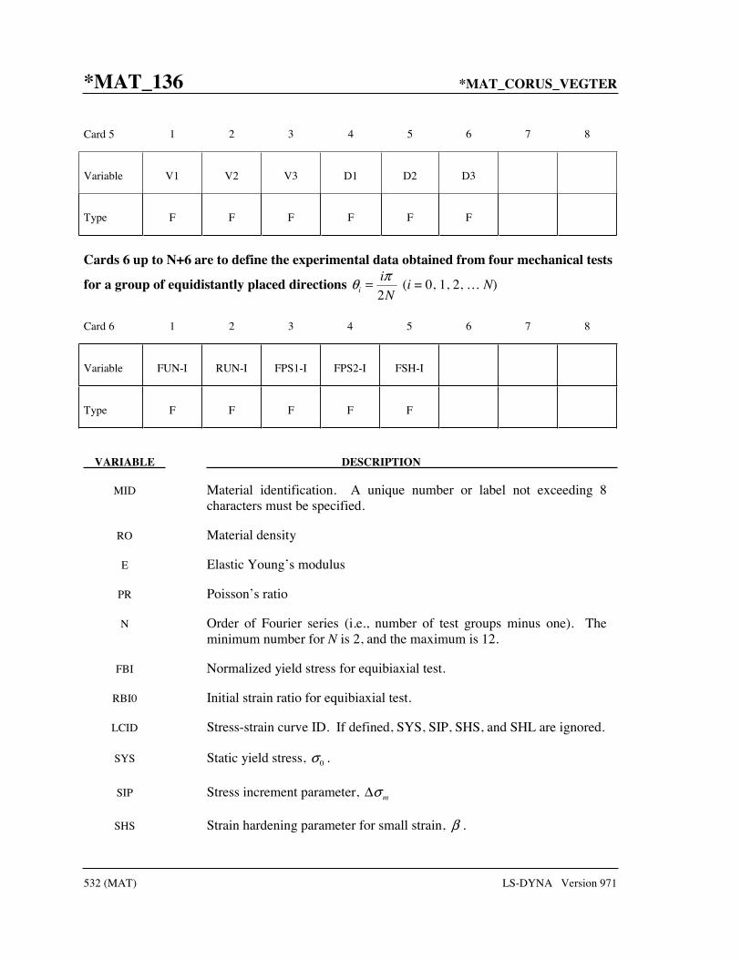
*MAT_136 *MAT_CORUS_VEGTER
532 (MAT) LS-DYNA Version 971
Card 5 1 2 3 4 5 6 7 8
Variable V1 V2 V3 D1 D2 D3
Type F F F F F F
Cards 6 up to N+6 are to define the experimental data obtained from four mechanical tests
for a group of equidistantly placed directions 2i
i
N
πθ = (i = 0, 1, 2, … N)
Card 6 1 2 3 4 5 6 7 8
Variable FUN-I RUN-I FPS1-I FPS2-I FSH-I
Type F F F F F
VARIABLE DESCRIPTION
MID Material identification. A unique number or label not exceeding 8 characters must be specified.
RO Material density
E Elastic Young’s modulus
PR Poisson’s ratio
N Order of Fourier series (i.e., number of test groups minus one). The minimum number for N is 2, and the maximum is 12.
FBI Normalized yield stress for equibiaxial test.
RBI0 Initial strain ratio for equibiaxial test.
LCID Stress-strain curve ID. If defined, SYS, SIP, SHS, and SHL are ignored.
SYS Static yield stress, 0σ .
SIP Stress increment parameter, mσΔ
SHS Strain hardening parameter for small strain, β .

*MAT_CORUS_VEGTER *MAT_136
LS-DYNA Version 971 533 (MAT)
VARIABLE DESCRIPTION
SHL Strain hardening parameter for larger strain, Ω .
ESH Exponent for strain hardening, n.
E0 Initial plastic strain
ALPHA α distribution of hardening used in the curve-fitting. 0α = pure kinematic hardening and 1α = provides pure isotropic hardening.
LCID2 Curve ID. The curve defines Young’s modulus change with respect to the plastic strain. By default it is assumed that Young’s modulus remains constant. Effective value is between 0-1.
AOPT Material axes option (see MAT_OPTION TROPIC_ELASTIC for a more complete description):
EQ.0.0: locally orthotropic with material axes determined by element nodes 1, 2, and 4, as with *DEFINE_COORDINATE_ NODES.
EQ.1.0: locally orthotropic with material axes determined by a point in space and the global location of the element center; this is the a-direction. This option is for solid elements only.
EQ.2.0: globally orthotropic with material axes determined by vectors defined below, as with *DEFINE_COORDINATE_ VECTOR.
EQ.3.0: locally orthotropic material axes determined by rotating the material axes about the element normal by an angle, BETA, from a line in the plane of the element defined by the cross product of the vector v with the element normal.
EQ.4.0: locally orthotropic in cylindrical coordinate system with the material axes determined by a vector v, and an originating point, P, which define the centerline axis. This option is for solid elements only.
LT.0.0: the absolute value of AOPT is a coordinate system ID number (CID on *DEFINE_COORDINATE_NODES, *DEFINE_ COORDINATE_SYSTEM or *DEFINE_COORDINATE_ VECTOR). Available in R3 version of 971 and later.
BETA Material angle in degrees for AOPT=3, may be overwritten on the element card, see *ELEMENT_SHELL_BETA or *ELEMENT_ SOLID_ORTHO.
XP YP ZP Coordinates of point p for AOPT = 1.
A1 A2 A3 Components of vector a for AOPT = 2.
V1 V2 V3 Components of vector v for AOPT = 3

*MAT_136 *MAT_CORUS_VEGTER
534 (MAT) LS-DYNA Version 971
VARIABLE DESCRIPTION
D1 D2 D3 Components of vector d for AOPT = 2.
FUN-I Normalized yield stress for uniaxial test for the ith direction.
RUN-I Strain ratio for uniaxial test for the ith direction.
FPS1-I First normalized yield stress for plain strain test for the ith direction.
FPS2-I Second normalized yield stress for plain strain test for the ith direction.
FSH-I First normalized yield stress for pure shear test for the ith direction.
Remarks:
The yield criterion is chosen as:
( )0 1 eqn
y m eq e εσ σ σ βε −Ω= + Δ + −

*MAT_COHESIVE_MIXED_MODE *MAT_138
LS-DYNA Version 971 535 (MAT)
*MAT_COHESIVE_MIXED_MODE
This is Material Type 138. This model is a simplification of *MAT_COHESIVE_GENERAL restricted to linear softening. It includes a bilinear traction-separation law with quadratic mixed mode delamination criterion and a damage formulation. It can be used with solid element types 19 and 20, and is not available for other solid element formulations. See the remarks after *SECTION_SOLID for a description of element types 19 and 20.
Card 1 1 2 3 4 5 6 7 8
Variable MID RO ROFLG INTFAIL EN ET GIC GIIC
Type A8 F F F F F F F
Card 2
Variable XMU T S UND UTD
Type F F F F F
VARIABLE DESCRIPTION
MID Material identification. A unique number or label not exceeding 8 characters must be specified.
RO Mass density
ROFLG Flag for whether density is specified per unit area or volume. ROFLG=0 specified density per unit volume (default), and ROFLG=1 specifies the density is per unit area for controlling the mass of cohesive elements with an initial volume of zero.
INTFAIL The number of integration points required for the cohesive element to be deleted. If it is zero, the element won’t be deleted even if it satisfies the failure criterion. The value of INTFAIL may range from 1 to 4, with 1 the recommended value.
EN The stiffness normal to the plane of the cohesive element.
ET The stiffness in the plane of the cohesive element.

*MAT_138 *MAT_COHESIVE_MIXED_MODE
536 (MAT) LS-DYNA Version 971
VARIABLE DESCRIPTION
GIC Energy release rate for mode I
GIIC Energy release rate for mode II
XMU Exponent of the mixed mode criteria (see remarks below)
T Peak traction in normal direction
S Peak traction in tangential direction
UND Ultimate displacement in the normal direction
UTD Ultimate displacement in the tangential direction
Remarks:
The ultimate displacements in the normal and tangential directions are the displacements at the time when the material has failed completely, i.e., the tractions are zero. The linear stiffness for loading followed by the linear softening during the damage provides an especially simple relationship between the energy release rates, the peak tractions, and the ultimate displacements:
2
2
GIC T UND /
GIIC S UTD /
= ⋅= ⋅
If the peak tractions aren’t specified, they are computed from the ultimate displacements. See Fiolka and Matzenmiller [2005] and Gerlach, Fiolka and Matzenmiller [2005].
In this cohesive material model, the total mixed-mode relative displacement mδ is
defined as 2 2m I IIδ δ δ= + , where 3Iδ δ= is the separation in normal direction (mode I) and
2 21 2IIδ δ δ= + is the separation in tangential direction (mode II). The mixed-mode damage
initiation displacement 0δ (onset of softening) is given by
( ) ( )2
0 0 02 20 0
1I II
II I
βδ δ δδ βδ
+=+
where 0 /I T ENδ = and 0 /II S ETδ = are the single mode damage inititation separations and
/II Iβ δ δ= is the “mode mixity” (see Figure 138.1). The ultimate mixed-mode displacement Fδ(total failure) for the power law (XMU>0) is:

*MAT_COHESIVE_MIXED_MODE *MAT_138
LS-DYNA Version 971 537 (MAT)
( )1
2 2
0
2 1XMUXMU XMU
F EN ET
GIC GIIC
β βδδ
−+ ⋅= +
and alternatively for the Benzeggagh-Kenane law [1996] (XMU<0):
( ) ( )2
2 2
2
20 11 1
2XMU
F ETGIC GIIC GIC
EN ETEN ETββ β
βδβδ
+ +
⋅= + −+ ⋅+
In this model, damage of the interface is considered, i.e. irreversible conditions are enforced with loading/unloading paths coming from/pointing to the origin.
Figure 138.1. Mixed-mode traction-separation law
Two error checks have been implemented for this material model in order to ensure proper material data. Since the traction versus displacement curve is fairly simple (triangular shaped), equations can be developed to ensure that the displacement (L) at the peak load (QMAX), is smaller than the ultimate distance for failure (u). See Figure 138.2 for the used notation.
One has that
1
2GC u QMAX= ⋅ and
QMAXL
E= .
To ensure that the peak is not past the failure point, u
L must be larger than 1.
GCu
EL
2= ,
Iδ
mδIIδ
S T
1β
Fδ
traction
FIIδ
0IIδ
FIδ
0Iδ
0δ
1
23

*MAT_138 *MAT_COHESIVE_MIXED_MODE
538 (MAT) LS-DYNA Version 971
Figure 138.2. Bilinear traction-separation law
where GC is the energy release rate. This gives
2
2 21
u GC GC
L ELL QMAXE
E
= = > .
The error checks are then done for tension and pure shear, respectively,
( )2
21
GICu
L TEN
EN
= > ,
( )2
21
GIICu
L SET
ET
= > .

*MAT_MODIFIED_FORCE_LIMITED *MAT_139
LS-DYNA Version 971 539 (MAT)
*MAT_MODIFIED_FORCE_LIMITED
This is Material Type 139. This material for the Belytschko-Schwer resultant beam is an extension of material 29. In addition to the original plastic hinge and collapse mechanisms of material 29, yield moments may be defined as a function of axial force. After a hinge forms, the moment transmitted by the hinge is limited by a moment-plastic rotation relationship.
Card 1 1 2 3 4 5 6 7 8
Variable MID RO E PR DF AOPT YTFLAG ASOFT
Type A8 F F F F F F F
Default none none none none 0.0 0.0 0.0 0.0
Card 2
Variable M1 M2 M3 M4 M5 M6 M7 M8
Type F F F F F F F F
Default none 0 0 0 0 0 0 0
Card 3
Variable LC1 LC2 LC3 LC4 LC5 LC6 LC7 LC8
Type F F F F F F F F
Default none 0 0 0 0 0 0 0
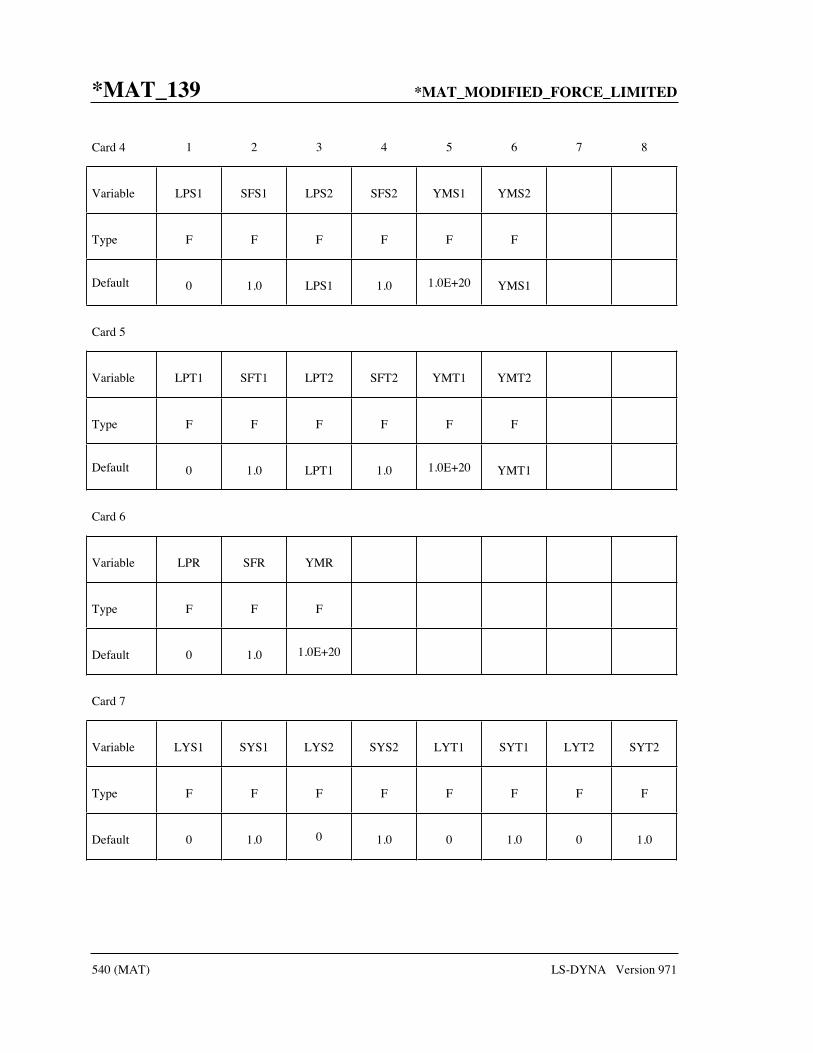
*MAT_139 *MAT_MODIFIED_FORCE_LIMITED
540 (MAT) LS-DYNA Version 971
Card 4 1 2 3 4 5 6 7 8
Variable LPS1 SFS1 LPS2 SFS2 YMS1 YMS2
Type F F F F F F
Default 0 1.0 LPS1 1.0 1.0E+20 YMS1
Card 5
Variable LPT1 SFT1 LPT2 SFT2 YMT1 YMT2
Type F F F F F F
Default 0 1.0 LPT1 1.0 1.0E+20 YMT1
Card 6
Variable LPR SFR YMR
Type F F F
Default 0 1.0 1.0E+20
Card 7
Variable LYS1 SYS1 LYS2 SYS2 LYT1 SYT1 LYT2 SYT2
Type F F F F F F F F
Default 0 1.0 0 1.0 0 1.0 0 1.0

*MAT_MODIFIED_FORCE_LIMITED *MAT_139
LS-DYNA Version 971 541 (MAT)
Card 8 1 2 3 4 5 6 7 8
Variable LYR SYR
Type F F
Default 0 1.0
Card 9
Variable HMS1_1 HMS1_2 HMS1_3 HMS1_4 HMS1_5 HMS1_6 HMS1_7 HMS1_8
Type F F F F F F F F
Default 0 0 0 0 0 0 0 0
Card 10
Variable LPMS1_1 LPMS1_2 LPMS1_3 LPMS1_4 LPMS1_5 LPMS1_6 LPMS1_7 LPMS1_8
Type F F F F F F F F
Default 0 0 0 0 0 0 0 0
Card 11
Variable HMS2_1 HMS2_2 HMS2_3 HMS2_4 HMS2_5 HMS2_6 HMS2_7 HMS2_8
Type F F F F F F F F
Default 0 0 0 0 0 0 0 0

*MAT_139 *MAT_MODIFIED_FORCE_LIMITED
542 (MAT) LS-DYNA Version 971
Card 12 1 2 3 4 5 6 7 8
Variable LPMS2_1 LPMS2_2 LPMS2_3 LPMS2_4 LPMS2_5 LPMS2_6 LPMS2_7 LPMS2_8
Type F F F F F F F F
Default 0 0 0 0 0 0 0 0
Card 13
Variable HMT1_1 HMT1_2 HMT1_3 HMT1_4 HMT1_5 HMT1_6 HMT1_7 HMT1_8
Type F F F F F F F F
Default 0 0 0 0 0 0 0 0
Card 14
Variable LPMT1_1 LPMT1_2 LPMT1_3 LPMT1_4 LPMT1_5 LPMT1_6 LPMT1_7 LPMT1_8
Type F F F F F F F F
Default 0 0 0 0 0 0 0 0
Card 15
Variable HMT2_1 HMT2_2 HMT2_3 HMT2_4 HMT2_5 HMT2_6 HMT2_7 HMT2_8
Type F F F F F F F F
Default 0 0 0 0 0 0 0 0

*MAT_MODIFIED_FORCE_LIMITED *MAT_139
LS-DYNA Version 971 543 (MAT)
Card 16 1 2 3 4 5 6 7 8
Variable LPMT2_1 LPMT2_2 LPMT2_3 LPMT2_4 LPMT2_5 LPMT2_6 LPMT2_7 LPMT2_8
Type F F F F F F F F
Default 0 0 0 0 0 0 0 0
Card 17
Variable HMR_1 HMR_2 HMR_3 HMR_4 HMR_5 HMR_6 HMR_7 HMR_8
Type F F F F F F F F
Default 0 0 0 0 0 0 0 0
Card 18
Variable LPMR_1 LPMR_2 LPMR_3 LPMR_4 LPMR_5 LPMR_6 LPMR_7 LPMR_8
Type F F F F F F F F
Default 0 0 0 0 0 0 0 0
VARIABLE DESCRIPTION
MID Material identification. A unique number or label not exceeding 8 characters must be specified.
RO Mass density
E Young’s modulus
PR Poisson’s ratio
DF Damping factor, see definition in notes below. A proper control for the timestep has to be maintained by the user!

*MAT_139 *MAT_MODIFIED_FORCE_LIMITED
544 (MAT) LS-DYNA Version 971
VARIABLE DESCRIPTION
AOPT Axial load curve option: EQ.0.0: axial load curves are force versus strain, EQ.1.0: axial load curves are force versus change in length. LT.0.0: the absolute value of AOPT is a coordinate system ID
number (CID on *DEFINE_COORDINATE_NODES, *DEFINE_ COORDINATE_SYSTEM or *DEFINE_COORDINATE_ VECTOR). Available in R3 version of 971 and later.
YTFLAG Flag to allow beam to yield in tension: EQ.0.0: beam does not yield in tension, EQ.1.0: beam can yield in tension.
ASOFT Axial elastic softening factor applied once hinge has formed. When a hinge has formed the stiffness is reduced by this factor. If zero, this factor is ignored.
M1, M2,...,M8 Applied end moment for force versus (strain/change in length) curve. At least one must be defined. A maximum of 8 moments can be defined. The values should be in ascending order.
LC1, LC2,...,LC8 Load curve ID (see *DEFINE_CURVE) defining axial force versus strain/change in length (see AOPT) for the corresponding applied end moment. Define the same number as end moments. Each curve must contain the same number of points.
LPS1 Load curve ID for plastic moment versus rotation about s-axis at node 1. If zero, this load curve is ignored.
SFS1 Scale factor for plastic moment versus rotation curve about s-axis at node 1. Default = 1.0.
LPS2 Load curve ID for plastic moment versus rotation about s-axis at node 2. Default: is same as at node 1.
SFS2 Scale factor for plastic moment versus rotation curve about s-axis at node 2. Default: is same as at node 1.
YMS1 Yield moment about s-axis at node 1 for interaction calculations (default set to 1.0E+20 to prevent interaction).
YMS2 Yield moment about s-axis at node 2 for interaction calculations (default set to YMS1).
LPT1 Load curve ID for plastic moment versus rotation about t-axis at node 1. If zero, this load curve is ignored.
SFT1 Scale factor for plastic moment versus rotation curve about t-axis at node 1. Default = 1.0.
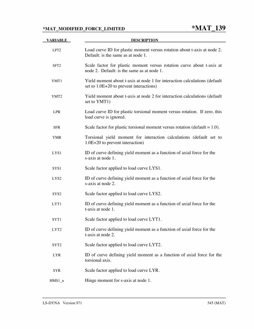
*MAT_MODIFIED_FORCE_LIMITED *MAT_139
LS-DYNA Version 971 545 (MAT)
VARIABLE DESCRIPTION
LPT2 Load curve ID for plastic moment versus rotation about t-axis at node 2.Default: is the same as at node 1.
SFT2 Scale factor for plastic moment versus rotation curve about t-axis at node 2. Default: is the same as at node 1.
YMT1 Yield moment about t-axis at node 1 for interaction calculations (default set to 1.0E+20 to prevent interactions)
YMT2 Yield moment about t-axis at node 2 for interaction calculations (default set to YMT1)
LPR Load curve ID for plastic torsional moment versus rotation. If zero, this load curve is ignored.
SFR Scale factor for plastic torsional moment versus rotation (default = 1.0).
YMR Torsional yield moment for interaction calculations (default set to 1.0E+20 to prevent interaction)
LYS1 ID of curve defining yield moment as a function of axial force for the s-axis at node 1.
SYS1 Scale factor applied to load curve LYS1.
LYS2 ID of curve defining yield moment as a function of axial force for the s-axis at node 2.
SYS2 Scale factor applied to load curve LYS2.
LYT1 ID of curve defining yield moment as a function of axial force for the t-axis at node 1.
SYT1 Scale factor applied to load curve LYT1.
LYT2 ID of curve defining yield moment as a function of axial force for the t-axis at node 2.
SYT2 Scale factor applied to load curve LYT2.
LYR ID of curve defining yield moment as a function of axial force for the torsional axis.
SYR Scale factor applied to load curve LYR.
HMS1_n Hinge moment for s-axis at node 1.

*MAT_139 *MAT_MODIFIED_FORCE_LIMITED
546 (MAT) LS-DYNA Version 971
VARIABLE DESCRIPTION
LPMS1_n ID of curve defining plastic moment as a function of plastic rotation for the s-axis at node 1 for hinge moment HMS1_n
HMS2_n Hinge moment for s-axis at node 2.
LPMS2_n ID of curve defining plastic moment as a function of plastic rotation for the s-axis at node 2 for hinge moment HMS2_n
HMT1_n Hinge moment for t-axis at node 1.
LPMT1_n ID of curve defining plastic moment as a function of plastic rotation for the t-axis at node 1 for hinge moment HMT1_n
HMT2_n Hinge moment for t-axis at node 2.
LPMT2_n ID of curve defining plastic moment as a function of plastic rotation for the t-axis at node 2 for hinge moment HMT2_n
HMR_n Hinge moment for the torsional axis.
LPMR_n ID of curve defining plastic moment as a function of plastic rotation for the torsional axis for hinge moment HMR_n
Remarks:
This material model is available for the Belytschko resultant beam element only. Plastic hinges form at the ends of the beam when the moment reaches the plastic moment. The plastic moment versus rotation relationship is specified by the user in the form of a load curve and scale factor. The points of the load curve are (plastic rotation in radians, plastic moment). Both quantities should be positive for all points, with the first point being (zero, initial plastic moment). Within this constraint any form of characteristic may be used, including flat or falling curves. Different load curves and scale factors may be specified at each node and about each of the local s and t axes.
Axial collapse occurs when the compressive axial load reaches the collapse load. Collapse load versus collapse deflection is specified in the form of a load curve. The points of the load curve are either (true strain, collapse force) or (change in length, collapse force). Both quantities should be entered as positive for all points, and will be interpreted as compressive. The first point should be (zero, initial collapse load).
The collapse load may vary with end moment as well as with deflections. In this case several load-deflection curves are defined, each corresponding to a different end moment. Each load curve should have the same number of points and the same deflection values. The end moment is defined as the average of the absolute moments at each end of the beam and is always positive.

*MAT_MODIFIED_FORCE_LIMITED *MAT_139
LS-DYNA Version 971 547 (MAT)
Stiffness-proportional damping may be added using the damping factor λ. This is defined as follows:
2 ξλω∗=
where ξ is the damping factor at the reference frequency ω (in radians per second). For example if 1% damping at 2Hz is required
2 0.010.001592
2 2λ
π∗= =
∗
If damping is used, a small time step may be required. LS-DYNA does not check this so to avoid instability it may be necessary to control the time step via a load curve. As a guide, the time step required for any given element is multiplied by 0.3L⁄cλ when damping is present (L = element length, c = sound speed).
Moment Interaction: Plastic hinges can form due to the combined action of moments about the three axes. This facility is activated only when yield moments are defined in the material input. A hinge forms when the following condition is first satisfied.
2 2 2
1r s t
ryield syield tyield
M M M
M M M+ + ≥
where,
Mr, Ms, Mt = current moment
Mryield, Msyield, Mtyield = yield moment
Note that scale factors for hinge behavior defined in the input will also be applied to the yield moments: for example, Msyield in the above formula is given by the input yield moment about the local axis times the input scale factor for the local s axis. For strain-softening characteristics, the yield moment should generally be set equal to the initial peak of the moment-rotation load curve.
On forming a hinge, upper limit moments are set. These are given by
,2
yield
upper
r
r r
MM MAX M=
and similar for Ms and Mt.
Thereafter the plastic moments will be given by
Mrp, = min (Mrupper, Mrcurve) and similar for s and t

*MAT_139 *MAT_MODIFIED_FORCE_LIMITED
548 (MAT) LS-DYNA Version 971
where
Mrp = current plastic moment
Mrcurve = moment taken from load curve at the current rotation scaled according to the scale factor.
The effect of this is to provide an upper limit to the moment that can be generated; it represents the softening effect of local buckling at a hinge site. Thus if a member is bent about is local s-axis it will then be weaker in torsion and about its local t-axis. For moments-softening curves, the effect is to trim off the initial peak (although if the curves subsequently harden, the final hardening will also be trimmed off).
It is not possible to make the plastic moment vary with the current axial load, but it is possible to make hinge formation a function of axial load and subsequent plastic moment a function of the moment at the time the hinge formed. This is discussed in the next section.
Independent plastic hinge formation:In addition to the moment interaction equation, Cards 7 through 18 allow plastic hinges
to form independently for the s-axis and t-axis at each end of the beam and also for the torsional axis. A plastic hinge is assumed to form if any component of the current moment exceeds the yield moment as defined by the yield moment vs. axial force curves input on cards 7 and 8. If any of the 5 curves is omitted, a hinge will not form for that component. The curves can be defined for both compressive and tensile axial forces. If the axial force falls outside the range of the curve, the first or last point in the curve will be used. A hinge forming for one component of moment does not effect the other components.
Upon forming a hinge, the magnitude of that component of moment will not be permitted to exceed the current plastic moment.. The current plastic moment is obtained by interpolating between the plastic moment vs. plastic rotation curves input on cards 10, 12, 14, 16, or 18. Curves may be input for up to 8 hinge moments, where the hinge moment is defined as the yield moment at the time that the hinge formed. Curves must be input in order of increasing hinge moment and each curve should have the same plastic rotation values. The first or last curve will be used if the hinge moment falls outside the range of the curves. If no curves are defined, the plastic moment is obtain from the curves on cards 4 through 6. The plastic moment is scaled by the scale factors on lines 4 to 6.
A hinge will form if either the independent yield moment is exceeded or if the moment interaction equation is satisfied. If both are true, the plastic moment will be set to the minimum of the interpolated value and Mrp.

*MAT_MODIFIED_FORCE_LIMITED *MAT_139
LS-DYNA Version 971 549 (MAT)
axial force
strains or change in length (see AOPT)
M1
2
4
8M
M
M
M
M
M
M
3
5
6
7
Figure 139.1. The force magnitude is limited by the applied end moment. For an intermediate value of the end moment LS-DYNA interpolates between the curves to determine the allowable force value.

*MAT_140 *MAT_VACUUM
550 (MAT) LS-DYNA Version 971
*MAT_VACUUM
This is Material Type 140. This model is a dummy material representing a vacuum in a multi-material Euler/ALE model. Instead of using ELFORM=12 (under *SECTION_SOLID), it is better to use ELFORM=11 with the void material defined as vacuum material instead.
Card 1 1 2 3 4 5 6 7 8
Variable MID RHO
Type A8 F
VARIABLE DESCRIPTION
MID Material identification. A unique number or label not exceeding 8 characters must be specified.
RHO Estimated material density. This is used only as stability check.
Remarks:
1. The vacuum density is estimated. It should be small relative to air in the model (possibly at least 310 to 610 lighter than air).

*MAT_RATE_SENSITIVE_POLYMER *MAT_141
LS-DYNA Version 971 551 (MAT)
*MAT_RATE_SENSITIVE_POLYMER
This is Material Type 141. This model is for the simulation of an isotropic ductile polymer with strain rate effects [Stouffer and Dame 1996]. Uniaxial test data has to be used.
Card 1 1 2 3 4 5 6 7 8
Variable MID RO E PR Do N Zo q
Type A8 F F F F F F F
Card 2
Variable Omega
Type F
VARIABLE DESCRIPTION
MID Material identification. A unique number or label not exceeding 8 characters must be specified.
RO Mass density
E Elastic modulus.
G Shear modulus
PR Poisson's ratio
Do Reference strain rate (=1000*max strain rate used in the test).
N Exponent (see inelastic strain rate equation below)
Zo Initial hardness of material
q (see equations below).
Omega Maximum internal stress.

*MAT_141 *MAT_RATE_SENSITIVE_POLYMER
552 (MAT) LS-DYNA Version 971
Remarks:
where the K2 term is defined as follows:
2 0.5( )( )ij ij ij ijK S S= − Ω − Ω
and represent the second invariant of the overstress tensor. The elastic components of the strain are added to the inelastic strain to obtain the total strain. The following relationship defines the internal stress variable rate:
2
3I I
ij m ij ij eq qε εΩ = Ω − Ω
where q is a material constant, Ωm is a material constant that represents the maximum value of
the internal stress, and Ieε is the effective inelastic strain. Also, see the LS-DYNA Theory
Manual for the procedure of calculation of the above parameters using series of tension tests under different strain rate.
2
2 2
exp 0.53
ε− Ω
= − ij ijoij o
SZD
K K

*MAT_TRANSVERSELY_ISOTROPIC_CRUSHABLE_FOAM *MAT_142
LS-DYNA Version 971 553 (MAT)
*MAT_TRANSVERSELY_ISOTROPIC_CRUSHABLE_FOAM
This is Material Type 142. This model is for an extruded foam material that is transversely isotropic, crushable, and of low density with no significant Poisson effect. This material is used in energy-absorbing structures to enhance automotive safety in low velocity (bumper impact) and medium high velocity (interior head impact and pedestrian safety) applications. The formulation of this foam is due to Hirth, Du Bois, and Weimar and is documented by Du Bois [2001]. This model behaves in a more physical way for off axis loading the material, *MAT_HONEYCOMB, which can exhibit nonphysical stiffening for loading conditions that are off axis. The load curves are used to define a yield surface that bounds the deviatoric stress tensor.
Card 1 1 2 3 4 5 6 7 8
Variable MID RO E11 E22 E12 E23 G K
Type A8 F F F F F F
Card 2
Variable I11 I22 I12 I23 IAA NY ANG MU
Type I I I I I I F F
Card 3
Variable AOPT ISCL MACF
Type F I I
Card 4
Variable XP YP ZP A1 A2 A3
Type F F F F F F

*MAT_142 *MAT_TRANSVERSELY_ISOTROPIC_CRUSHABLE_FOAM
554 (MAT) LS-DYNA Version 971
Card 5 1 2 3 4 5 6 7 8
Variable D1 D2 D3 V1 V2 V3
Type F F F F F F
VARIABLE DESCRIPTION
MID Material identification. A unique number or label not exceeding 8 characters must be specified.
RO Mass density
E11 Elastic modulus in axial direction.
E22 Elastic modulus in transverse direction (E22=E33).
E12 Elastic shear modulus (E12=E31).
E23 Elastic shear modulus in transverse plane.
G Shear modulus.
K Bulk modulus for contact stiffness.
I11 Load curve for nominal axial stress versus volumetric strain.
I22 Load curve ID for nominal transverse stresses versus volumetric strain (I22=I33).
I12 Load curve ID for shear stress component 12 and 31 versus volumetric strain (I12=I31).
I23 Load curve ID for shear stress component 23 versus volumetric strain.
IAA Load curve ID (optional) for nominal stress versus volumetric strain for load at angle, ANG, relative to the material axis.
NY Set to unity for a symmetric yield surface.
ANG Angle corresponding to load curve ID, IAA.

*MAT_TRANSVERSELY_ISOTROPIC_CRUSHABLE_FOAM *MAT_142
LS-DYNA Version 971 555 (MAT)
VARIABLE DESCRIPTION
MU Damping coefficient for tensor viscosity which acts in both tension and compression. Recommended values vary between 0.05 to 0.10. If zero, tensor viscosity is not used, but bulk viscosity is used instead. Bulk viscosity creates a pressure as the element compresses that is added to the normal stresses, which can have the effect of creating transverse deformations when none are expected.
AOPT Material axes option (see MAT_OPTION TROPIC_ELASTIC for a more complete description):
EQ.0.0: locally orthotropic with material axes determined by element nodes as shown in Figure 2.1. Nodes 1, 2, and 4 of an element are identical to the nodes used for the definition of a coordinate system as by *DEFINE_COORDINATE_NODES.
EQ.1.0: locally orthotropic with material axes determined by a point in space and the global location of the element center; this is the a-direction. This option is for solid elements only.
EQ.2.0: globally orthotropic with material axes determined by vectors defined below, as with *DEFINE_COORDINATE_ VECTOR.
EQ.3.0: locally orthotropic material axes determined by rotating the material axes about the element normal by an angle, BETA, from a line in the plane of the element defined by the cross product of the vector v with the element normal. The plane of a solid element is the midsurface between the inner surface and outer surface defined by the first four nodes and the last four nodes of the connectivity of the element, respectively.
EQ.4.0: locally orthotropic in cylindrical coordinate system with the material axes determined by a vector v, and an originating point, P, which define the centerline axis. This option is for solid elements only.
LT.0.0: the absolute value of AOPT is a coordinate system ID number (CID on *DEFINE_COORDINATE_NODES, *DEFINE_ COORDINATE_SYSTEM or *DEFINE_COORDINATE_ VECTOR). Available in R3 version of 971 and later.
ISCL Load curve ID for the strain rate scale factor versus the volumetric strain rate. The yield stress is scaled by the value specified by the load curve.
MACF Material axes change flag: EQ.1: No change, default, EQ.2: switch material axes a and b, EQ.3: switch material axes a and c, EQ.4: switch material axes b and c.
XP YP ZP Coordinates of point p for AOPT = 1 and 4.

*MAT_142 *MAT_TRANSVERSELY_ISOTROPIC_CRUSHABLE_FOAM
556 (MAT) LS-DYNA Version 971
VARIABLE DESCRIPTION
A1 A2 A3 Components of vector a for AOPT = 2.
D1 D2 D3 Components of vector d for AOPT = 2.
V1 V2 V3 Define components of vector v for AOPT = 3 and 4.
Remarks:
Tensor viscosity, which is activated by a nonzero value for MU, is generally more stable than bulk viscosity. A damping coefficient less than 0.01 has little effect, and a value greater than 0.10 may cause numerical instabilities.

*MAT_WOOD *MAT_143
LS-DYNA Version 971 557 (MAT)
*MAT_WOOD_{OPTION}
This is Material Type 143. This is a transversely isotropic material and is available for solid elements. The user has the option of inputting his or her own material properties (<BLANK>), or requesting default material properties for Southern yellow pine (PINE) or Douglas fir (FIR).This model was developed by Murray [2002] under a contract from the FHWA.
Available options include:
<BLANK>
PINE
FIR
Card 1 1 2 3 4 5 6 7 8
Variable MID RO NPLOT ITERS IRATE GHARD IFAIL IVOL
Type A8 F I I I F I I
Define the following card for the PINE and FIR options.
Card 2 1 2 3 4 5 6 7 8
Variable MOIS TEMP QUAL_T QUAL_C UNITS IQUAL
Type F F F F I I
Define the following cards, 2-6, for the <BLANK> option.
Card 2 1 2 3 4 5 6 7 8
Variable EL ET GLT GTR PR
Type F F F F F

*MAT_143 *MAT_WOOD
558 (MAT) LS-DYNA Version 971
Card 3 1 2 3 4 5 6 7 8
Variable XT XC YT YC SXY SYZ
Type F F F F F F
Card 4
Variable GF1|| GF2|| BFIT DMAX|| GF1⊥ GF2⊥ DFIT DMAX⊥
Type F F F F F F F F
Card 5
Variable FLPAR FLPARC POWPAR FLPER FLPERC POWPER
Type F F F F F F
Card 6
Variable NPAR CPAR NPER CPER
Type F F F F
Define the following three cards for all options.
Card 3/7 1 2 3 4 5 6 7 8
Variable AOPT MACF BETA
Type F I F

*MAT_WOOD *MAT_143
LS-DYNA Version 971 559 (MAT)
Card 4/8 1 2 3 4 5 6 7 8
Variable XP YP ZP A1 A2 A3
Type F F F F F F
Card 5/9
Variable D1 D2 D3 V1 V2 V3
Type F F F F F F
VARIABLE DESCRIPTION
MID Material identification. A unique number or label not exceeding 8 characters must be specified.
RO Mass density
NPLOT Controls what is written as component 7 to the d3plot database. LS-PrePost always blindly labels this component as effective plastic strain.:
EQ.1: Parallel damage (default). EQ.2: Perpendicular damage.
ITERS Number of plasticity algorithm iterations. The default is one iteration.
IRATE Rate effects option: EQ.0: Rate effects model turned off (default). EQ.1: Rate effects model turned on.
GHARD Perfect plasticity override. Values greater than or equal to zero are allowed. Positive values model late time hardening in compression (an increase in strength with increasing strain). A zero value models perfect plasticity (no increase in strength with increasing strain). The default is zero.
IFAIL Erosion perpendicular to the grain. EQ.0: No (default). EQ.1: Yes (not recommended except for debugging).
IVOL Erode on negative volume or strain increments greater than 0.01. EQ.0: No, do not apply erosion criteria. EQ.1: Yes, apply volume and strain erosion criteria.

*MAT_143 *MAT_WOOD
560 (MAT) LS-DYNA Version 971
VARIABLE DESCRIPTION
MOIS Percent moisture content. If left blank, moisture content defaults to saturated at 30%.
TEMP Temperature in ˚C. If left blank, temperature defaults to room temperature at 20 ˚C
QUAL_T Quality factor options. These quality factors reduce the clear wood tension, shear, and compression strengths as a function of grade.
EQ.0: Grade 1, 1D, 2, 2D. Predefined strength reduction factors are: Pine: Qual_T=0.47 in tension/shear. Qual_C=0.63 in compression. Fir: Qual_T=0.40 in tension/shear Qual_C=0.73 in compression. EQ.-1: DS-65 or SEl STR (pine and fir). Predefined strength reduction factors are: Qual_T=0.80 in tension/shear. Qual_C=0.93 in compression. EQ.-2: Clear wood. No strength reduction factors are applied: Qual_T=1.0. Qual_C=1.0. GT.0: User defined quality factor in tension. Values between 0 and
1 are expected. Values greater than one are allowed, but may not be realistic.
QUAL_C User defined quality factor in compression. This input value is used if Qual_T>0. Values between 0 and 1 are expected. Values greater than one are allowed, but may not be realistic. If left blank, a default value of Qual_C=Qual_T is used.
UNITS Units options:
EQ.0: GPa, mm, msec, Kg/mm3, kN. EQ.1: MPa, mm, msec, g/mm3, Nt. EQ.2: MPa, mm, sec, Mg/mm3, Nt. EQ.3: Psi, inch, sec, lb-s2/inch4, lb
IQUAL Apply quality factors perpendicular to the grain: EQ.0: Yes (default). EQ 1: No.
EL Parallel normal modulus
ET Perpendicular normal modulus.
GLT Parallel shear modulus (GLT=GLR).

*MAT_WOOD *MAT_143
LS-DYNA Version 971 561 (MAT)
VARIABLE DESCRIPTION
GTR Perpendicular shear modulus.
PR Parallel major Poisson's ratio.
XT Parallel tensile strength.
XC Parallel compressive strength.
YT Perpendicular tensile strength.
YC Perpendicular compressive strength.
SXY Parallel shear strength.
SYZ Perpendicular shear strength.
GF1|| Parallel fracture energy in tension.
GF2|| Parallel fracture energy in shear.
BFIT Parallel softening parameter.
DMAX|| Parallel maximum damage.
GF1⊥ Perpendicular fracture energy in tension.
GF2⊥ Perpendicular fracture energy in shear.
DFIT Perpendicular softening parameter.
DMAX⊥ Perpendicular maximum damage.
FLPAR Parallel fluidity parameter for tension and shear.
FLPARC Parallel fluidity parameter for compression.
POWPAR Parallel power.
FLPER Perpendicular fluidity parameter for tension and shear.
FLPERC Perpendicular fluidity parameter for compression.
POWPER Perpendicular power.
NPAR Parallel hardening initiation.
CPAR Parallel hardening rate

*MAT_143 *MAT_WOOD
562 (MAT) LS-DYNA Version 971
VARIABLE DESCRIPTION
NPER Perpendicular hardening initiation.
CPER Perpendicular hardening rate.
AOPT Material axes option (see MAT_OPTION TROPIC_ELASTIC for a more complete description):
EQ.0.0: locally orthotropic with material axes determined by element nodes as shown in Figure 2.1. Nodes 1, 2, and 4 of an element are identical to the nodes used for the definition of a coordinate system as by *DEFINE_COORDINATE_NODES.
EQ.1.0: locally orthotropic with material axes determined by a point in space and the global location of the element center; this is the a-direction. This option is for solid elements only.
EQ.2.0: globally orthotropic with material axes determined by vectors defined below, as with *DEFINE_COORDINATE_ VECTOR.
EQ.3.0: locally orthotropic material axes determined by rotating the material axes about the element normal by an angle, BETA, from a line in the plane of the element defined by the cross product of the vector v with the element normal. The plane of a solid element is the midsurface between the inner surface and outer surface defined by the first four nodes and the last four nodes of the connectivity of the element, respectively.
EQ.4.0: locally orthotropic in cylindrical coordinate system with the material axes determined by a vector v, and an originating point, P, which define the centerline axis. This option is for solid elements only.
LT.0.0: the absolute value of AOPT is a coordinate system ID number (CID on *DEFINE_COORDINATE_NODES, *DEFINE_ COORDINATE_SYSTEM or *DEFINE_COORDINATE_ VECTOR). Available in R3 version of 971 and later.
MACF Material axes change flag: EQ.1: No change, default, EQ.2: switch material axes a and b, EQ.3: switch material axes a and c, EQ.4: switch material axes b and c.
BETA Material angle in degrees for AOPT = 3, may be overridden on the element card, see *ELEMENT_ SOLID_ORTHO.
XP YP ZP Coordinates of point p for AOPT = 1 and 4.

*MAT_WOOD *MAT_143
LS-DYNA Version 971 563 (MAT)
VARIABLE DESCRIPTION
A1 A2 A3 Components of vector a for AOPT = 2.
D1 D2 D3 Components of vector d for AOPT = 2.
V1 V2 V3 Define components of vector v for AOPT = 3 and 4.
Remarks:
Material property data is for clear wood (small samples without defects like knots), whereas real structures are composed of graded wood. Clear wood is stronger than graded wood. Quality factors (strength reduction factors) are applied to the clear wood strengths to account for reductions in strength as a function of grade. One quality factor (Qual_T) is applied to the tensile and shear strengths. A second quality factor (Qual_C) is applied to the compressive strengths. As a option, predefined quality factors are provided based on correlations between LS-DYNA calculations and test data for pine and fir posts impacted by bogie vehicles. By default, quality factors are applied to both the parallel and perpendicular to the grain strengths. An option is available (IQUAL) to eliminate application perpendicular to the grain.

*MAT_144 *MAT_PITZER_CRUSHABLE_FOAM
564 (MAT) LS-DYNA Version 971
*MAT_PITZER_CRUSHABLE_FOAM
This is Material Type 144. This model is for the simulation of isotropic crushable forms with strain rate effects. Uniaxial and triaxial test data have to be used. For the elastic response, the Poisson ratio is set to zero.
Card 1 1 2 3 4 5 6 7 8
Variable MID RO K G PR TY SRTV
Type A8 F F F F F F
Card 2
Variable LCPY LCUYS LCSR VC DFLG
Type I I I F F
VARIABLE DESCRIPTION
MID Material identification. A unique number or label not exceeding 8 characters must be specified.
RO Mass density
K Bulk modulus.
G Shear modulus
PR Poisson's ratio
TY Tension yield.
SRTV Young’s modulus (E)
LCPY Load curve ID giving pressure versus volumetric strain, see Figure 75.1.
LCUYS Load curve ID giving uniaxial stress versus volumetric strain, see Figure 75.1.
LCSR Load curve ID giving strain rate scale factor versus volumetric strain rate.

*MAT_PITZER_CRUSHABLE_FOAM *MAT_144
LS-DYNA Version 971 565 (MAT)
VARIABLE DESCRIPTION
VC Viscous damping coefficient (.05 <recommended value < .50).
DFLG Density flag: EQ.0.0: use initial density EQ.1.0: use current density (larger step size with less mass scaling).
Remarks:
The logarithmic volumetric strain is defined in terms of the relative volume, V , as:
γ = − ln(V )
In defining the curves the stress and strain pairs should be positive values starting with a volumetric strain value of zero.

*MAT_145 *MAT_SCHWER_MURRAY_CAP_MODEL
566 (MAT) LS-DYNA Version 971
*MAT_SCHWER_MURRAY_CAP_MODEL
This is Material Type 145. The Schwer & Murray Cap Model, known as the Continuous Surface Cap Model, is a three invariant extension of the Geological Cap Model (Material Type 25) that also includes viscoplasticity for rate effects and damage mechanics to model strain softening. The primary references are Schwer and Murray [1994], Schwer [1994], and Murray and Lewis [1994]. The model is appropriate for geomaterials including soils, concrete, and rocks.
Warning: no default input parameter values are assumed, but recommendations for the more obscure parameters are provided in the descriptions that follow.
Card 1 1 2 3 4 5 6 7 8
Variable MID RO SHEAR BULK GRUN SHOCK PORE
Type A8 F F F F F F
Card 2
Variable ALPHA THETA GAMMA BETA EFIT FFIT ALPHAN CALPHA
Type F F F F F F F F
Card 3
Variable RO XO IROCK SECP AFIT BFIT RDAMO
Type F F F F F F F

*MAT_SCHWER_MURRAY_CAP_MODEL *MAT_145
LS-DYNA Version 971 567 (MAT)
Card 4 1 2 3 4 5 6 7 8
Variable W D1 D2 NPLOT EPSMAX CFIT DFIT TFAIL
Type F F F F F F F F
Card 5
Variable FAILFL DBETA DDELTA VPTAU
Type F F F F
Card 6
Variable ALPHA1 THETA1 GAMMA1 BETA1 ALPHA2 THETA2 GAMMA2 BETA2
Type F F F F F F F F
VARIABLE DESCRIPTION
MID Material identification. A unique number or label not exceeding 8 characters must be specified.
RO Mass density
SHEAR Shear modulus, G
BULK Bulk modulus, K
GRUN Gruneisen ratio (typically = 0), Γ
SHOCK Shock velocity parameter (typically 0), Sl
PORE Flag for pore collapse EQ.0.0: for Pore collapse EQ.1.0: for Constant bulk modulus (typical)
ALPHA Shear failure parameter, α
THETA Shear failure parameter, θ

*MAT_145 *MAT_SCHWER_MURRAY_CAP_MODEL
568 (MAT) LS-DYNA Version 971
VARIABLE DESCRIPTION
GAMMA Shear failure parameter, γ
BETA Shear failure parameter, β
2 1 1 1( ) exp( )eJ F J J Jα γ β θ′ = = − − +
EFIT Dilitation damage mechanics parameter (no damage = 1)
FFIT Dilitation damage mechanics parameter (no damage = 0)
ALPHAN Kinematic strain hardening parameter, Nα
CALPHAN Kinematic strain hardening parameter, cα
R0 Initial cap surface ellipticity, R
X0 Initial cap surface 1J (mean stress) axis intercept, X(κ 0 )
IROCK EQ.0: soils (cap can contract) EQ.1: rock/concrete
SECP Shear enhanced compaction
AFIT Ductile damage mechanics parameter (=1 no damage)
BFIT Ductile damage mechanics parameter (=0 no damage)
RDAM0 Ductile damage mechanics parameter
W Plastic Volume Strain parameter, W
D1 Plastic Volume Strain parameter, D1
D2 Plastic Volume Strain parameter, D2
( ) ( ( ) )( )2
1 0 2 01 exp ( ) ( ) ( )PV W D X X D X Xε κ κ κ κ= − − − − −
NPLOT History variable post-processed as effective plastic strain (See Table 145.1 for history variables available for plotting)
EPSMAX Maximum permitted strain increment (default = 0)
max
10.05( ) min ,
9
RN
G Kαε α γΔ = − − (calculated default)
CFIT Brittle damage mechanics parameter (=1 no damage)

*MAT_SCHWER_MURRAY_CAP_MODEL *MAT_145
LS-DYNA Version 971 569 (MAT)
VARIABLE DESCRIPTION
DFIT Brittle damage mechanics parameter (=0 no damage)
TFAIL Tensile failure stress
FAILFL Flag controlling element deletion and effect of damage on stress (see Remarks 1 and 2):
EQ.1: σ ij reduces with increasing damage; element is deleted when
fully damaged (default) EQ.-1: σ ij reduces with increasing damage; element is not deleted
EQ.2: ijS reduces with increasing damage; element is deleted when
fully damaged EQ.-2: ijS reduces with increasing damage; element is not deleted
DBETA Rounded vertices parameter, Δβ0
DDELTA Rounded vertices parameter, δ
VPTAU Viscoplasticity relaxation time parameter, τ
ALPHA1 Torsion scaling parameter,α1
1 10α α< → = Friction Angle (degrees)
THETA1 Torsion scaling parameter, θ1
GAMMA1 Torsion scaling parameter, γ 1
BETA1 Torsion scaling parameter, β1
1 1 1 1 1 1 1exp( )Q J Jα γ β θ= − − +
ALPHA2 Tri-axial extension scaling parameter, α2
THETA2 Tri-axial extension scaling parameter, θ2
GAMMA2 Tri-axial extension scaling parameter, γ 2
BETA2 Tri-axial extension scaling parameter, β2
2 2 2 2 1 2 1exp( )Q J Jα γ β θ= − − +
Remarks:
1. FAILFL controls whether the damage accumulation applies to either the total stress tensorσ ij or the deviatoric stress tensor ijS . When FAILFL = 2, damage does not
diminish the ability of the material to support hydrostatic stress.
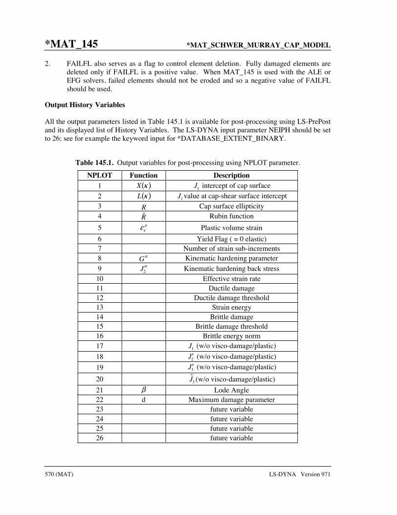
*MAT_145 *MAT_SCHWER_MURRAY_CAP_MODEL
570 (MAT) LS-DYNA Version 971
2. FAILFL also serves as a flag to control element deletion. Fully damaged elements are deleted only if FAILFL is a positive value. When MAT_145 is used with the ALE or EFG solvers, failed elements should not be eroded and so a negative value of FAILFL should be used.
Output History Variables
All the output parameters listed in Table 145.1 is available for post-processing using LS-PrePost and its displayed list of History Variables. The LS-DYNA input parameter NEIPH should be set to 26; see for example the keyword input for *DATABASE_EXTENT_BINARY.
Table 145.1. Output variables for post-processing using NPLOT parameter.
NPLOT Function Description 1 X κ( ) J1 intercept of cap surface
2 L κ( ) J1 value at cap-shear surface intercept 3 R Cap surface ellipticity 4 R Rubin function
5 pνε Plastic volume strain
6 Yield Flag ( = 0 elastic) 7 Number of strain sub-increments 8 Gα Kinematic hardening parameter
9 J2α Kinematic hardening back stress
10 Effective strain rate 11 Ductile damage 12 Ductile damage threshold 13 Strain energy 14 Brittle damage 15 Brittle damage threshold 16 Brittle energy norm 17 J1 (w/o visco-damage/plastic)
18 ′ J2 (w/o visco-damage/plastic)
19 ′ J3 (w/o visco-damage/plastic)
20 J3 (w/o visco-damage/plastic)
21 β Lode Angle 22 d Maximum damage parameter 23 future variable 24 future variable 25 future variable 26 future variable

*MAT_SCHWER_MURRAY_CAP_MODEL *MAT_145
LS-DYNA Version 971 571 (MAT)
Sample Input for Concrete Gran and Senseny [1996] report the axial stress versus strain response for twelve unconfined compression tests of concrete, used in scale-model reinforced-concrete wall tests. The Schwer & Murray Cap Model parameters provided below were used, see Schwer [2001], to model the unconfined compression test stress-strain response for the nominal 40 MPa strength concrete reported by Gran and Senseny. The basic units for the provided parameters are length in millimeters (mm), time in milliseconds (msec), and mass in grams (g). This base unit set yields units of force in Newtons (N) and pressure in Mega-Pascals (MPa).
Keyword:
Card 1 1 2 3 4 5 6 7 8
Variable MID RO SHEAR BULK GRUN SHOCK PORE
Type A8 2.3E-3 1.048E4 1.168E4 0.0 0.0 1.
Card 2 1 2 3 4 5 6 7 8
Variable ALPHA THETA GAMMA BETA EFIT FFIT ALPHAN CALPHA
Type 190.0 0.0 184.2 2.5E-3 0.999 0.7 2.5 2.5E3
Card 3 1 2 3 4 5 6 7 8
Variable R0 X0 IROCK SECP AFIT BFIT RDAM0
Type 5.0 100.0 1.0 0.0 0.999 0.3 0.94
Card 4 1 2 3 4 5 6 7 8
Variable W D1 D2 NPLOT EPSMAX CFIT DFIT TFAIL
Type 5.0E-2 2.5E-4 3.5E-7 23.0 0.0 1.0 300.0 13.8
Card 5 1 2 3 4 5 6 7 8
Variable FAILFG DBETA DDELTA VPTAU
Type 1.0 0.0 0.0 0.0
Card 6 1 2 3 4 5 6 7 8
Variable ALPHA1 THETA1 GAMMA1 BETA1 ALPHA2 THETA2 GAMMA2 BETA2
Type 0.747 3.3E-4 0.17 5.0E-2 0.66 4.0E-4 0.16 5.0E-2
User Input Parameters and System of Units
Consider the following basic units:
Length - L (e.g. millimeters - mm ) Mass - M (e.g. grams - g ) Time - T (e.g. milliseconds - ms )
The following consistent unit systems can then be derived using Newton's Law, i.e. F Ma= .

*MAT_145 *MAT_SCHWER_MURRAY_CAP_MODEL
572 (MAT) LS-DYNA Version 971
Force - 2/F ML T= [ g-mm/ms 2 = Kg-m/s 2 = Newton - N ] and
Stress - 2/F Lσ = [ N/mm 2 = 10 6 N/m 2 = 10 6 Pascals = MPa ] and
Density - 3/M Lρ = [ g/mm 3 = 10 6 Kg/m 3 ]
User Inputs and Units:
Card 1 1 2 3 4 5 6 7 8 Variable MID RO SHEAR BULK GRUN SHOCK PORE
Units I Density M/L 3
StressF/L 2
StressF/L 2
Card 2 1 2 3 4 5 6 7 8 Variable ALPHA THETA GAMMA BETA EFIT FFIT ALPHAN CALPHA
Units Stress F/L 2
StressF/L 2
1
2
Stress
/F L
− 1/ 2
2
Stress
/F L
− StressF/L 2
Stress F/L 2
Card 3 1 2 3 4 5 6 7 8 Variable R0 X0 IROCK SECP AFIT BFIT RDAM0
Units StressF/L 2
1/ 2
2
Stress
/F L
− 1/ 2
2
Stress
/F L
Card 4 1 2 3 4 5 6 7 8 Variable W D1 D2 NPLOT MAXEPS CFIT DFIT TFAIL
Units 1
2
Stress
/F L
− 2
2
Stress
/F L
− 1/ 2
2
Stress
/F L
− Stress F/L 2
Card 5 1 2 3 4 5 6 7 8 Variable FAILFG DBETA DDELTA VPTAU
Units Angle degrees
Time T
Card 6 1 2 3 4 5 6 7 8 Variable ALPHA1 THETA1 GAMMA1 BETA1 ALPHA2 THETA2 GAMMA2 BETA2
Units Stress F/L 2
StressF/L 2
1
2
Stress
/F L
− StressF/L 2
StressF/L 2
1
2
Stress
/F L
−

*MAT_1DOF_GENERALIZED_SPRING *MAT_146
LS-DYNA Version 971 573 (MAT)
*MAT_1DOF_GENERALIZED_SPRING
This is Material Type 146. This is a linear spring or damper that allows different degrees-of-freedom at two nodes to be coupled.
Card 1 1 2 3 4 5 6 7 8
Variable MID RO K C SCLN1 SCLN2 DOFN1 DOFN2
Type A8 F F F F F I I
Card 2
Variable CID1 CID2
Type I I
VARIABLE DESCRIPTION
MID Material identification. A unique number or label not exceeding 8 characters must be specified.
RO Mass density, see also volume in *SECTION_BEAM definition.
K Spring stiffness.
C Damping constant.
SCLN1 Scale factor on force at node 1. Default=1.0.
SCLN2 Scale factor on force at node 2. Default=1.0.
DOFN1 Active degree-of-freedom at node 1, a number between 1 to 6 where 1 in x-translation and 4 is x-rotation. If this parameter is defined in the SECTION_BEAM definition or on the ELEMENT_BEAM_SCALAR card, then the value here, if defined, is ignored.
DOFN2 Active degree-of-freedom at node 2, a number between 1 to 6. If this parameter is defined in the SECTION_BEAM definition or on the ELEMENT_BEAM_SCALAR card, then the value here, if defined, is ignored.

*MAT_146 *MAT_1DOF_GENERALIZED_SPRING
574 (MAT) LS-DYNA Version 971
VARIABLE DESCRIPTION
CID1 Local coordinate system at node 1. This coordinate system can be overwritten by a local system specified on the *ELEMENT_BEAM _SCALAR or *SECTION_BEAM keyword input. If no coordinate system is specified, the global system is used.
CID2 Local coordinate system at node 2. If CID2=0, CID2=CID1.

*MAT_FHWA_SOIL *MAT_147
LS-DYNA Version 971 575 (MAT)
*MAT_FHWA_SOIL
This is Material Type 147. This is an isotropic material with damage and is available for solid elements. The model has a modified Mohr-Coulomb surface to determine the pressure dependent peak shear strength. It was developed for applications involving roadbase soils by Lewis [1999] for the FHWA, who extended the work of Abbo and Sloan [1995] to include excess pore water effects.
Card 1 1 2 3 4 5 6 7 8
Variable MID RO NPLOT SPGRAV RHOWAT VN GAMMAR INTRMX
Type A8 F I F F F F I
Default none none 1 none 1.0 0.0 0.0 1
Card 2
Variable K G PHIMAX AHYP COH ECCEN AN ET
Type F F F F F F
Default none none none none none none none none
Card 3
Variable MCONT PWD1 PWKSK PWD2 PHIRES DINT VDFM DAMLEV
Type F F F F F F F F
Default none none none none 0.0 none none none

*MAT_147 *MAT_FHWA_SOIL
576 (MAT) LS-DYNA Version 971
Card 4 1 2 3 4 5 6 7 8
Variable EPSMAX
Type F
Default none
VARIABLE DESCRIPTION
MID Material identification. A unique number or label not exceeding 8 characters must be specified.
RO Mass density
NPLOT Controls what is written as component 7 to the d3plot database. LS-Prepost always blindly labels this component as effective plastic strain.
EQ.1: Effective Strain EQ.2: Damage Criterion Threshold EQ.3: Damage (diso) EQ.4: Current Damage Criterion EQ.5: Pore Water Pressure EQ.6: Current Friction Angle (phi)
SPGRAV Specific Gravity of Soil used to get porosity.
RHOWAT Density of water in model units - used to determine air void strain (saturation)
VN Viscoplasticity parameter (strain-rate enhanced strength)
GAMMAR Viscoplasticity parameter (strain-rate enhanced strength)
ITERMAX Maximum number of plasticity iterations (default 1)
K Bulk Modulus (non-zero)
G Shear modulus (non-zero)
PHIMAX Peak Shear Strength Angle (friction angle) (radians)
AHYP Coefficient A for modified Drucker-Prager Surface
COH Cohesion ñ Shear Strength at zero confinement (overburden)

*MAT_FHWA_SOIL *MAT_147
LS-DYNA Version 971 577 (MAT)
VARIABLE DESCRIPTION
ECCEN Eccentricity parameter for third invariant effects
AN Strain hardening percent of phi max where non-linear effects start
ET Strain Hardening Amount of non-linear effects
MCONT Moisture Content of Soil (Determines amount of air voids) (0-1.00)
PWD1 Parameter for pore water effects on bulk modulus
PWKSK Skeleton bulk modulus- Pore water parameter ñ set to zero to eliminate effects
PWD2 Parameter for pore water effects on the effective pressure (confinement)
PHIRES The minimum internal friction angle, radians (residual shear strength)
DINT Volumetric Strain at Initial damage threshold, EMBED Equation.3
VDFM Void formation energy (like fracture energy)
DAMLEV Level of damage that will cause element deletion (0.0-1.0)
EPSMAX Maximum principle failure strain

*MAT_147_N *MAT_FHWA_SOIL_NEBRASKA
578 (MAT) LS-DYNA Version 971
*MAT_FHWA_SOIL_NEBRASKA
This is an option to use the default properties determined for soils used at the University of Nebraska (Lincoln). The default units used for this material are millimeter, millisecond, and kilograms. If different units are desired, the conversion factors must be input.
This is Material Type 147. This is an isotropic material with damage and is available for solid elements. The model has a modified Mohr-Coulomb surface to determine the pressure dependent peak shear strength. It was developed for applications involving road base soils.
Card 1 1 2 3 4 5 6 7 8
Variable MID FCTIM FCTMAS FCTLEN
Type A8 F I F F F F I
Default none none 1 none 1.0 0.0 0.0 1
VARIABLE DESCRIPTION
MID Material identification. A unique number or label not exceeding 8 characters must be specified.
FCTIM Factor to multiply milliseconds by to get desired time units
FCTMAS Factor to multiply kilograms by to get desired mass units
FCTLEN Factor to multiply millimeters by to get desired length units

*MAT_GAS_MIXTURE *MAT_148
LS-DYNA Version 971 579 (MAT)
*MAT_GAS_MIXTURE
This is Material Type 148. This model is for the simulation of thermally equilibrated ideal gas mixtures. This only works with the multi-material ALE formulation (ELFORM=11 in *SECTION_SOLID). This keyword needs to be used together with *INITIAL_GAS_MIXTURE for the initialization of gas densities and temperatures. When applied in the context of ALE airbag modeling, the injection of inflator gas is done with a *SECTION_POINT_SOURCE_ MIXTURE command which controls the injection process. This material model type also has its name start with *MAT_ALE_. For example, an identical material model to this is *MAT_ALE_GAS_MIXTURE (or also, *MAT_ALE_03).
Card 1
Card 1 1 2 3 4 5 6 7 8
Variable MID IADIAB RUNIV
Type A8 I F
Default none 0 0.0
Remark 5 1
Card 2: Method (A) RUNIV=BLANK or 0.0 Per-mass unit is used
Card 2 1 2 3 4 5 6 7 8
Variable CVmass1 CVmass2 CVmass3 CVmass4 CVmass5 CVmass6 CVmass7 CVmass8
Type F F F F F F F F
Default none none none none none none none none
Remark

*MAT_148 *MAT_GAS_MIXTURE
580 (MAT) LS-DYNA Version 971
Card 3: Method (A) RUNIV=BLANK or 0.0 Per-mass unit is used
Card 3 1 2 3 4 5 6 7 8
Variable CPmass1 CPmass 2 CPmass 3 CPmass 4 CPmass 5 CPmass6 CPmass 7 CPmass 8
Type F F F F F F F F
Default none none none none none none none none
Remark
Card 2: Method (B) RUNIV is nonzero
Card 2 1 2 3 4 5 6 7 8
Variable MOLWT1 MOLWT 2 MOLWT 3 MOLWT 4 MOLWT 5 MOLWT 6 MOLWT 7 MOLWT 8
Type F F F F F F F F
Default none none none none none none none none
Remark 2
Card 3: Method (B) RUNIV is nonzero Per-mole unit is used
Card 3 1 2 3 4 5 6 7 8
Variable CPmole1 CPmole2 CPmole3 CPmole4 CPmole5 CPmole6 CPmole7 CPmole8
Type F F F F F F F F
Default none none none none none none none none
Remark 2

*MAT_GAS_MIXTURE *MAT_148
LS-DYNA Version 971 581 (MAT)
Card 4: Method (B) RUNIV is nonzero
Card 4 1 2 3 4 5 6 7 8
Variable B1 B2 B3 B4 B5 B6 B7 B8
Type F F F F F F F F
Default none none none none none none none none
Remark 2
Card 5: Method (B) RUNIV is nonzero
Card 5 1 2 3 4 5 6 7 8
Variable C1 C2 C3 C4 C5 C6 C7 C8
Type F F F F F F F F
Default none none none none none none none none
Remark 2
VARIABLE DESCRIPTION
MID Material identification. A unique number or label not exceeding 8 characters must be specified.
IADIAB This flag (default=0) is used to turn ON/OFF adiabatic compression logics for an ideal gas (remark 5).
EQ.0: OFF (default) EQ.1: ON
RUNIV Universal gas constant in per-mole unit (8.31447 J/(mole*K)).
CVmass1-CVmass8 If RUNIV is BLANK or zero (method A): Heat capacity at constant volume for up to eight different gases in per-mass unit.
CPmass1-CPmass8 If RUNIV is BLANK or zero (method A): Heat capacity at constant pressure for up to eight different gases in per-mass unit.

*MAT_148 *MAT_GAS_MIXTURE
582 (MAT) LS-DYNA Version 971
VARIABLE DESCRIPTION
MOLWT1-MOLWT8 If RUNIV is nonzero (method B): Molecular weight of each ideal gas in the mixture (mass-unit/mole).
CPmole1-CPmole8 If RUNIV is nonzero (method B): Heat capacity at constant pressure for up to eight different gases in per-mole unit. These are nominal heat capacity values typically at STP. These are denoted by the variable “A” in the equation in remark 2.
B1-B8 If RUNIV is nonzero (method B): First order coefficient for a temperature dependent heat capacity at constant pressure for up to eight different gases. These are denoted by the variable “B” in the equation in remark 2.
C1-C8 If RUNIV is nonzero (method B): Second order coefficient for a temperature dependent heat capacity at constant pressure for up to eight different gases. These are denoted by the variable “C” in the equation in remark 2.
Remarks:
1. There are 2 methods of defining the gas properties for the mixture. If RUNIV is BLANK or ZERO Method (A) is used to define constant heat capacities where per-mass unit values of Cv and Cp are input. Only cards 2 and 3 are required for this method. Method (B) is used to define constant or temperature dependent heat capacities where per-mole unit values of Cp are input. Cards 2-5 are required for this method.
2. The per-mass-unit, temperature-dependent, constant-pressure heat capacity is
2
0
[ * * ]( ) ~
*
~ ( * )
p
P
A B T C T JC T
MW kg K
A C J mole K
+ +=
=
2
3
~ ( * )
~ ( * )
B J mole K
C J mole K
The units shown are only for demonstration of the equation.
3. The initial temperature and the density of the gas species present in a mesh or part at time zero is specified by the keyword *INITIAL_GAS_MIXTURE.
4. The ideal gas mixture is assumed to be thermal equilibrium, that is, all species are at the same temperature (T). The gases in the mixture are also assumed to follow Dalton’s
Partial Pressure Law, =ngas
iiPP . The partial pressure of each gas is then TRP
igasii ρ=
where univgasi
RR
MW= . The individual gas species temperature equals the mixture
temperature. The temperature is computed from the internal energy where the mixture internal energy per unit volume is used,

*MAT_GAS_MIXTURE *MAT_148
LS-DYNA Version 971 583 (MAT)
i i
i
ngas ngas
V i V i i Vi i
Vi ngas
i Vi
e C T C T
eT T
C
ρ ρ
ρ
= =
= =.
In general, the advection step conserves momentum and internal energy, but not kinetic energy. This can result in energy lost in the system and lead to a pressure drop. In *MAT_GAS_MIXTURE the dissipated kinetic energy is automatically converted into heat (internal energy). Thus in effect the total energy is conserved instead of conserving just the internal energy. This numerical scheme has been shown to improve accuracy in some cases. However, the user should always be vigilant and check the physics of the problem closely.
5. As an example consider an airbag surrounded by ambient air. As the inflator gas flows into the bag, the ALE elements cut by the airbag fabric shell elements will contain some inflator gas inside and some ambient air outside. The multi-material element treatment is not perfect. Consequently the temperature of the outside air may be made artificially high after the multi-material element treatment. To prevent the outside ambient air from getting artificially high T, set IDIAB=1 for the ambient air outside. Simple adiabatic compression equation is then assumed for the outside air. The use of this flag may be needed, but only when that air is modeled by the *MAT_GAS_MIXTURE card.
Example:
Consider a tank test model where the Lagrangian tank (Part S1) is surrounded by an ALE air mesh (Part H4=AMMGID 1). There are 2 ALE parts which are defined but initially have no corresponding mesh: part 5 (H5=AMMGID 2) is the resident gas inside the tank at t = 0, and part 6 (H6=AMMGID 2) is the inflator gas(es) which is injected into the tank when t > 0. AMMGID stands for ALE Multi-Material Group ID. Please see figure and input below. The *MAT_GAS_MIXTURE (MGM) card defines the gas properties of ALE parts H5 & H6. The MGM card input for both method (A) and (B) are shown.
The *INITIAL_GAS_MIXTURE card is also shown. It basically specifies that “AMMGID 2 may be present in part or mesh H4 at t=0, and the initial density of this gas is defined in the rho1 position which corresponds to the 1st material in the mixture (or H5, the resident gas).”

*MAT_148 *MAT_GAS_MIXTURE
584 (MAT) LS-DYNA Version 971
Example configuration:
Sample input:
$-------------------------------------------------------------------------------*PARTH5 = initial gas inside the tank $ PID SECID MID EOSID HGID GRAV ADPOPT TMID 5 5 5 0 5 0 0 *SECTION_SOLID 5 11 0 $-------------------------------------------------------------------------------$ Example 1: Constant heat capacities using per-mass unit. $*MAT_GAS_MIXTURE$ MID IADIAB R_univ $ 5 0 0$ Cv1_mas Cv2_mas Cv3_mas Cv4_mas Cv5_mas Cv6_mas Cv7_mas Cv8_mas $718.7828911237.56228$ Cp1_mas Cp2_mas Cp3_mas Cp4_mas Cp5_mas Cp6_mas Cp7_mas Cp8_mas $1007.00058 1606.1117 $-------------------------------------------------------------------------------$ Example 2: Variable heat capacities using per-mole unit. *MAT_GAS_MIXTURE$ MID IADIAB R_univ 5 0 8.314470 $ MW1 MW2 MW3 MW4 MW5 MW6 MW7 MW8 0.0288479 0.02256 $ Cp1_mol Cp2_mol Cp3_mol Cp4_mol Cp5_mol Cp6_mol Cp7_mol Cp8_mol 29.049852 36.23388 $ B1 B2 B3 B4 B5 B6 B7 B8 7.056E-3 0.132E-1 $ C1 C2 C3 C4 C5 C6 C7 C8 -1.225E-6 -0.190E-5 $-------------------------------------------------------------------------------$ One card is defined for each AMMG that will occupy some elements of a mesh set *INITIAL_GAS_MIXTURE$ SID STYPE MMGID T0 4 1 1 298.15 $ RHO1 RHO2 RHO3 RHO4 RHO5 RHO6 RHO7 RHO8 1.17913E-9*INITIAL_GAS_MIXTURE$ SID STYPE MMGID T0 4 1 2 298.15 $ RHO1 RHO2 RHO3 RHO4 RHO5 RHO6 RHO7 RHO8 1.17913E-9$-------------------------------------------------------------------------------
S1= tank
H4=AMMG1=background outside air (initially defined ALE mesh)
H5=AMMG2=initial gas inside the tank (this has no initial mesh)
H6=AMMG2=inflator gas(es) injected in (this has no initial mesh)
Cut-off view

*MAT_EMMI *MAT_151
LS-DYNA Version 971 585 (MAT)
*MAT_EMMI
This is Material Type 151. The Evolving Microstructural Model of Inelasticity (EMMI) is a temperature and rate-dependent state variable model developed to represent the large deformation of metals under diverse loading conditions [Marin 2005].
Card 1 1 2 3 4 5 6 7 8
Variable MID RHO E PR
Type A8 F F F
Default - - - - - - -
Card 2
Variable RGAS BVECT D0 QD CV ADRAG BDRAG DMTHETA
Type F F F F F F F F
Default - - - - - - - -
Card 3
Variable DMPHI DNTHETA DNPHI THETA0 THETAM BETA0 BTHETA DMR
Type F F F F F F F F
Default - - - - - - - -

*MAT_151 *MAT_EMMI
586 (MAT) LS-DYNA Version 971
Card 4 1 2 3 4 5 6 7 8
Variable DM1 DM2 DM3 DM4 DM5 Q1ND Q2ND Q3ND
Type I F F F F F F
Default - - - - - - -
Card 5
Variable Q4ND CALPHA CKAPPA C1 C2ND C3 C4 C5
Type F F F F F F F F
Default - - - - - - - -
Card 6
Variable C6 C7ND C8ND C9ND C10 A1 A2 A3
Type F F F F F F F F
Default - - - - - - - -

*MAT_EMMI *MAT_151
LS-DYNA Version 971 587 (MAT)
Card 7 1 2 3 4 5 6 7 8
Variable A4 A_XX A_YY A_ZZ A_XY A_YZ A_XZ ALPHXX
Type F F F F F F F F
Default - - - - - - -
Card 8
Variable ALPHYY ALPHZZ ALPHXY ALPHYZ ALPHXZ DKAPPA PHI0 DLBDAG
Type F F F F F F F F
Default - - - - - - - -
Card 9
Variable FACTOR DMGOPT DELASO DIMPLO ATOL RTOL DNITER XTRA1
Type F F F F F F F F
Default - - - - - - - -

*MAT_151 *MAT_EMMI
588 (MAT) LS-DYNA Version 971
Card 10 1 2 3 4 5 6 7 8
Variable XTRA2 XTRA3 XTRA4 XTRA5 XTRA6 XTRA7 XTRA8 XTRA9
Type I F F F F F F
Default - - - - - - -
Card 11
Variable XTRA10 XTRA11 XTRA12 XTRA13 XTRA14 XTRA15 XTRA16 XTRA17
Type F F F F F F F F
Default - - - - - - - -
VARIABLE DESCRIPTION
MID Material identification. A unique number or label not exceeding 8 characters must be specified.
RHO Material density.
E Young’s modulus
PR Poisson’s ratio
RGAS universal gas constant.
BVECT Burger’s vector
D0 pre-exponential diffusivity coefficient
QD activation energy
CV specific heat at constant volume
ADRAG drag intercept
BDRAG drag coefficient

*MAT_EMMI *MAT_151
LS-DYNA Version 971 589 (MAT)
VARIABLE DESCRIPTION
DMTHETA shear modulus temperature coefficient
DMPHI shear modulus damage coefficient
DNTHETA bulk modulus temperature coefficient
DNPHI bulk modulus damage coefficient
THETA0 reference temperature
THETAM melt temperature
BETA0 coefficient of thermal expansion at reference temperature
BTHETA thermal expansion temperature coefficient
DMR damage rate sensitivity parameter
DM1 coefficient of yield temperature dependence
DM2 coefficient of yield temperature dependence
DM3 coefficient of yield temperature dependence
DM4 coefficient of yield temperature dependence
DM5 coefficient of yield temperature dependence
Q1ND dimensionless activation energy for f
Q2ND dimensionless activation energy for rd
Q3ND dimensionless activation energy for Rd
Q4ND dimensionless activation energy Rs
CALPHA coefficient for backstress alpha
CKAPPA coefficient for internal stress kappa
C1 parameter for flow rule exponent n
C2ND parameter for transition rate f
C3 parameter for alpha dynamic recovery rd
C4 parameter for alpha hardening h
C5 parameter for kappa dynamic recovery Rd

*MAT_151 *MAT_EMMI
590 (MAT) LS-DYNA Version 971
VARIABLE DESCRIPTION
C6 parameter for kappa hardening H
C7ND parameter kappa static recovery Rs
C8ND parameter for yield
C9ND parameter for temperature dependence of flow rule exponent n
C10 parameter for static recovery (set=1)
A1 plastic anisotropy parameter
A2 plastic anisotropy parameter
A3 plastic anisotropy parameter
A4 plastic anisotropy parameter
A_XX initial structure tensor component
A_YY initial structure tensor component
A_ZZ initial structure tensor component
A_XY initial structure tensor component
A_YZ initial structure tensor component
A_XZ initial structure tensor component
ALPHXX initial backstress component
ALPHYY initial backstress component
ALPHZZ initial backstress component
ALPHXY initial backstress component
ALPHYZ initial backstress component
ALPHXZ initial backstress component
DKAPPA initial isotropic internal stress
PHI0 initial isotropic porosity
DLBDAG slip system geometry parameter
FACTOR fraction of plastic work converted to heat, adiabatic
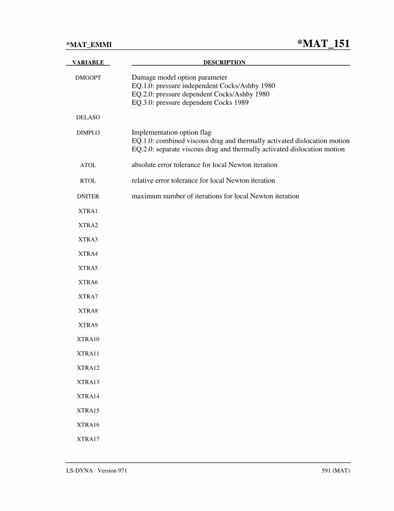
*MAT_EMMI *MAT_151
LS-DYNA Version 971 591 (MAT)
VARIABLE DESCRIPTION
DMGOPT Damage model option parameter EQ.1.0: pressure independent Cocks/Ashby 1980 EQ.2.0: pressure dependent Cocks/Ashby 1980 EQ.3.0: pressure dependent Cocks 1989
DELASO
DIMPLO Implementation option flag EQ.1.0: combined viscous drag and thermally activated dislocation motion
EQ.2.0: separate viscous drag and thermally activated dislocation motion
ATOL absolute error tolerance for local Newton iteration
RTOL relative error tolerance for local Newton iteration
DNITER maximum number of iterations for local Newton iteration
XTRA1
XTRA2
XTRA3
XTRA4
XTRA5
XTRA6
XTRA7
XTRA8
XTRA9
XTRA10
XTRA11
XTRA12
XTRA13
XTRA14
XTRA15
XTRA16
XTRA17

*MAT_151 *MAT_EMMI
592 (MAT) LS-DYNA Version 971
Remarks:
p pdh r ε α
∇= −dα α
( ) ( )sinhpd s sH R R Qκ κ ε κ κ= − −
3 sinh 1
2p p p n, f
Y
σε εκ
= = −+
d n
Table 151.1. Plasticity Material Functions of EMMI Model. equationpε − equation−α equationκ −
12 exp
Qf c
θ= 2
3 expd
Qr c
θ−= 3
5 expd
QR c
θ−=
91
cn c
θ= − ( )4h c μ θ= ( )6H c μ θ=
( )8Y c Y θ= 47 exps
QR c
θ−=
510 exps
QQ c
θ−=
Void growth:
( ) ( )31 , ,
2p
eqG pϕ ϕ σ ϕ ε= −
( ) ( )( )2 2 13 1
, , 1 sinh1 1 2 13
eqeq
m pG p
m mτσ ϕϕ σ
−= −
− + +

*MAT_DAMAGE_3 *MAT_153
LS-DYNA Version 971 593 (MAT)
*MAT_DAMAGE_3
This is Material Type 153. This model has two back stress terms for kinematic hardening combined with isotropic hardening and a damage model for modeling low cycle fatigue and failure. Huang [2006] programmed this model and provided it as a user subroutine with the documentation that follows. It is available for beam, shell and solid elements. This material model is available starting with the R3 release of Version 971.
Card 1 1 2 3 4 5 6 7 8
Variable MID RO E PR SIGY HARDI BETA LCSS
Type A8 F F F F F F I
Card 2
Variable HARDK1 GAMMA1 HARDK2 GAMMA2
Type F F F F
Card 3
Variable IDAMAGE IDS IDEP EPSD S T DC
Type I I I F F F F
VARIABLE DESCRIPTION
MID Material identification. A unique number or label not exceeding 8 characters must be specified.
RO Mass density, ρ
E Young’s modulus, E
PR Poisson’s ratio, v
SIGY Initial yield stress, 0yσ
HARDI Isotropic hardening modulus, H

*MAT_153 *MAT_DAMAGE_3
594 (MAT) LS-DYNA Version 971
VARIABLE DESCRIPTION
BETA Isotropic hardening parameter, β . Set 0β = for linear isotropic hardening.
LCSS Load curve ID defining effective stress vs. effective plastic strain
HARDK1 Kinematic hardening modulus 1C
GAMMA1 Kinematic hardening parameter 1γ
HARDK2 Kinematic hardening modulus 2C
GAMMA2 Kinematic hardening parameter 2γ
IDAMAGE Isotropic damage flag EQ. 0: damage is inactivated EQ. 1: damage is activated
IDS Output stress flag EQ. 0: undamaged stress is σ output EQ. 1: damaged stress is ( )1 Dσ − output
IDEP Damaged plastic strain
EQ. 0: plastic strain is accumulated plr ε=
EQ. 1: damaged plastic strain is accumulated ( )1 plr D ε= −
EPSD Damage threshold dr . Damage accumulation begins when dr r>
S Damage material constant S. Default = 0 200yσ
T Damage material constant t. Default = 1
DC Critical damage value cD . When damage value reaches critical, the
element is deleted from calculation. Default = 0.5
Remarks:
This model is based on the work of Lemaitre [1992], and Dufailly and Lemaitre [1995]. It is a pressure-independent plasticity model with the yield surface defined by the function
0yF σ σ= − =
where vσ is uniaxial yield stress

*MAT_DAMAGE_3 *MAT_153
LS-DYNA Version 971 595 (MAT)
( )0 1 expy y
Hrσ σ β
β= + − −
By setting 0β = , a linear isotropic hardening is obtained
0y y Hrσ σ= +
where 0vσ s the initial yield stress. And σ is the equivalent von Mises stress, with respect to the
deviatoric effective stress
[ ]e dev= − = −s s
where s is deviatoric stress and is the back stress, which is decomposed into several components
jj
=
and is effective stress (undamaged stress), based on Continuum Damage Mechanics model [Lemaitre 1992]
1 D=
−
where D is the isotropic damage scalar, which is bounded by 0 and 1
0 1D≤ ≤
D = 0 represents a damage-free material RVE (representative Volume Element), while D = 1 represents a fully broken material RVE in two parts. In fact, fracture occurs when 1cD D= < ,
modeled as element removal. The evolution of the isotropic damage value related to ductile damage and fracture (the case where the plastic strain or dissipation is much larger than the elastic one, [Lemaitre 1992]) is defined as
1&
3
0
σεσ
> > −=
tpl m
deq
Yr r
D S
otherwise
where m
eq
σσ
is the stress triaxiality, dr is damage threshold, S is a material constant, and Y is
strain energy release rate.
: :el el elY = D

*MAT_153 *MAT_DAMAGE_3
596 (MAT) LS-DYNA Version 971
Where elD represents the fourth-order elasticity tensor, el is elastic strain. And t is a material constant, introduced by Dufailly and Lemaitre [1995], to provide additional degree of freedom for modeling low-cycle fatigue ( 1=t in Lemaitre [1992]). Dufailly and Lemaitre [1995] also proposed a simplified method to fit experimental results and get S and t.
The equivalent Mises stress is defined as
( ) 3 3:
2 2e e e eσ = =s s s s
The model assumes associated plastic flow
3
2pl eF
d dλ λσ
∂= =∂
s
Where dλ is the plastic consistency parameter. The evolution of the kinematic component of the model is defined as [Armstrong and Frederick 1966]:
( )
2IDEP=0
32
1 IDEP=13
pl plj j j j
pl plj j j j
C
D C
γ ε
γ ε
= −
= − −
The damaged plastic strain is accumulated as
( )IDEP=0
1 IDEP=1
pl
pl
r
r D
ε
ε
=
= −
where plε is the equivalent plastic strain rate
2:
3pl pl plε =
where pl represents the rate of plastic flow.
Table 153.1 shows the difference between MAT 153 and MAT 104/105. MAT 153 is less computationally expensive than MAT 104/105. Kinematic hardening, which already exists in MAT 103, is included in MAT 153, but not in MAT 104/105.

*MAT_DAMAGE_3 *MAT_153
LS-DYNA Version 971 597 (MAT)
Table 153.1 Difference between MAT 153 and MAT 104/105
MAT 153 MAT 104 MAT 105
Computational cost 1.0 3.0 3.0
Isotropic hardening One component Two components One component
Kinematic hardening Two components N/A N/A
Output stress σ IDS=0
( )1 Dσ − IDS=1 ( )1 Dσ − ( )1 Dσ −
Damaged plastic strain
plr ε= IDEP=0
( )1 plr D ε= − IDEP=1 ( )1 plr D ε= − ( )1 plr D ε= −
Accumulation when 1
3m
eq
σσ
> −1 0σ > 1 0σ >
Isotropic plasticity Yes Yes Yes
Anisotropic plasticity No Yes No
Isotropic damage Yes Yes Yes
Anisotropic damage No Yes No

*MAT_154 *MAT_DESHPANDE_FLECK_FOAM
598 (MAT) LS-DYNA Version 971
*MAT_DESHPANDE_FLECK_FOAM
This is material type 154 for solid elements. This material is for modeling aluminum foam used as a filler material in aluminum extrusions to enhance the energy absorbing capability of the extrusion. Such energy absorbers are used in vehicles to dissipate energy during impact. This model was developed by Reyes, Hopperstad, Berstad, and Langseth [2002] and is based on the foam model by Deshpande and Fleck [2000].
Card 1 1 2 3 4 5 6 7 8
Variable MID RHO E PR ALPHA GAMMA
Type A8 F F F F F
Default - - - - - -
Card 2
Variable EPSD ALPHA2 BETA SIGP DERFI CFAIL
Type F F F F F F
Default - - - - - -
VARIABLE DESCRIPTION
MID Material identification. A unique number or label not exceeding 8 characters must be specified.
RHO Mass density.
E Young’s modulus.
PR Poisson’s ratio.
ALPHA Controls shape of yield surface.
GAMMA See remarks.
EPSD Densification strain.

*MAT_DESHPANDE_FLECK_FOAM *MAT_154
LS-DYNA Version 971 599 (MAT)
VARIABLE DESCRIPTION
ALPHA2 See remarks.
BETA See remarks.
SIGP See remarks.
DERFI Type of derivation used in material subroutine EQ.0: Numerical derivation EQ.1: Analytical derivation
CFAIL Failure strain.
The yield stress function Φ is defined by:
Φ = σ −σ y
The equivalent stress σ is given by:
2 2 22
2
13
VM mσ α σσα
+=+
where, VMσ , is the von Mises effective stress:
2:
3dev dev
VMσ σ σ=
In this equation σ m and σ dev are the mean and deviatoric stress:
σ dev = σ − σm I
The yield stress σ y can be expressed as:
2
1ln
1
y pD
D
βεσ σ γ αε ε
ε
= + +
−
Here, σ p , α 2 , γ and β are material parameters. The densification strain ε D is defined as:

*MAT_154 *MAT_DESHPANDE_FLECK_FOAM
600 (MAT) LS-DYNA Version 971
ε D = − lnρ f
ρf 0
where ρ f is the foam density and ρ f 0 is the density of the virgin material.

*MAT_PLASTICITY_COMPRESSION_TENSION_EOS *MAT_155
LS-DYNA Version 971 601 (MAT)
*MAT_PLASTICITY_COMPRESSION_TENSION_EOS
This is Material Type 155. An isotropic elastic-plastic material where unique yield stress versus plastic strain curves can be defined for compression and tension. Also, failure can occur based on a plastic strain or a minimum time step size. Rate effects on the yield stress are modeled either by using the Cowper-Symonds strain rate model or by using two load curves that scale the yield stress values in compression and tension, respectively. Material rate effects, which are independent of the plasticity model, are based on a 6-term Prony series Maxwell mode that generates an additional stress tensor. The viscous stress tensor is superimposed on the stress tensor generated by the plasticity. Pressure is defined by an equation of state, which is required to utilize this model. This model is for solid elements only.
Card 1 1 2 3 4 5 6 7 8
Variable MID RO E PR C P FAIL TDEL
Type A8 F F F F F F F
Default none none none none 0 0 10.E+20 0
Card 2
Variable LCIDC LCIDT LCSRC LCSRT SRFLAG
Type I I I I F
Default 0 0 0 0 0
Card 3
Variable PC PT PCUTC PCUTT PCUTF
Type F F F F F
Default 0 0 0 0 0

*MAT_155 *MAT_PLASTICITY_COMPRESSION_TENSION_EOS
602 (MAT) LS-DYNA Version 971
Card 4 1 2 3 4 5 6 7 8
Variable K
Type F
Card Format for viscoelastic constants. Up to 6 cards may be input. A keyword card (with a “*” in column 1) terminates this input if less than 6 cards are used.
Optional Cards
1 2 3 4 5 6 7 8
Variable GI BETAI
Type F F
VARIABLE DESCRIPTION
MID Material identification. A unique number or label not exceeding 8 characters must be specified.
RO Mass density.
E Young’s modulus.
PR Poisson’s ratio.
C Strain rate parameter, C, see formula below.
P Strain rate parameter, P, see formula below.
FAIL Failure flag. LT.0.0: User defined failure subroutine is called to determine
failure EQ.0.0: Failure is not considered. This option is recommended if
failure is not of interest since many calculations will be saved. GT.0.0: Plastic strain to failure. When the plastic strain reaches
this value, the element is deleted from the calculation.
TDEL Minimum time step size for automatic element deletion.
LCIDC Load curve ID defining yield stress versus effective plastic strain in compression.

*MAT_PLASTICITY_COMPRESSION_TENSION_EOS *MAT_155
LS-DYNA Version 971 603 (MAT)
VARIABLE DESCRIPTION
LCIDT Load curve ID defining yield stress versus effective plastic strain in tension.
LCSRC Optional load curve ID defining strain rate scaling effect on yield stress when the material is in compression.
LCSRT Optional load curve ID defining strain rate scaling effect on yield stress when the material is in tension.
SRFLAG Formulation for rate effects: EQ.0.0: Total strain rate, EQ.1.0: Deviatoric strain rate.
PC Compressive mean stress (pressure) at which the yield stress follows load curve ID, LCIDC. If the pressure falls between PC and PT a weighted average of the two load curves is used.
PT Tensile mean stress at which the yield stress follows load curve ID, LCIDT.
PCUTC Pressure cut-off in compression.
PCUTT Pressure cut-off in tension.
PCUTF Pressure cut-off flag. EQ.0.0: Inactive, EQ.1.0: Active.
K Optional bulk modulus for the viscoelastic material. If nonzero a Kelvin type behavior will be obtained. Generally, K is set to zero.
GI Optional shear relaxation modulus for the ith term
BETAI Optional shear decay constant for the ith term
Remarks:
The stress strain behavior follows a different curve in compression than it does in tension. Tension is determined by the sign of the mean stress where a positive mean stress (i.e., a negative pressure) is indicative of tension. Two curves must be defined giving the yield stress versus effective plastic strain for both the tension and compression regimes.

*MAT_156 *MAT_MUSCLE
604 (MAT) LS-DYNA Version 971
*MAT_MUSCLE
This is material type 156 for truss elements. This material is a Hill-type muscle model with activation and a parallel damper. Also, see *MAT_SPRING_MUSCLE where a description of the theory is available.
Card 1 1 2 3 4 5 6 7 8
Variable MID RO SNO SRM PIS SSM CER DMP
Type A8 F F F F F F F
Default
Card 2
Variable ALM SFR SVS SVR SSP
Type F F F F F
Default 0.0 1.0 1.0 1.0 0.0
VARIABLE DESCRIPTION
MID Material identification. A unique number or label not exceeding 8 characters must be specified.
RO Material density in the initial undeformed configuration.
SNO Initial stretch ratio, 0
l
l, i.e., the current length as defined by the nodal
points at t=0 divided by the initial length. The density for the nodal
mass calculation is RO/SNO, or 0l
l
ρ.
SRM Maximum strain rate.
PIS Peak isometric stress corresponding to the dimensionless value of unity in the dimensionless stress versus strain function, see SSP below.

*MAT_MUSCLE *MAT_156
LS-DYNA Version 971 605 (MAT)
VARIABLE DESCRIPTION
SSM Strain when the dimensionless stress versus strain function, SSP below, reaches its maximum stress value.
CER Constant, governing the exponential rise of SSP. Required if SSP=0.
DMP Damping constant.
ALM Activation level vs. time. LT.0: absolute value gives load curve ID GE.0: constant value of ALM is used
SFR Scale factor for strain rate maximum vs. the stretch ratio, 0
l
l.
LT.0: absolute value gives load curve ID GE.0: constant value of 1.0 is used
SVS Active dimensionless tensile stress vs. the stretch ratio, 0
l
l.
LT.0: absolute value gives load curve ID GE.0: constant value of 1.0 is used
TV Active dimensionless tensile stress vs. the normalized strain rate, 0
l
l.
LT.0: absolute value gives load curve ID GE.0: constant value of 1.0 is used
SSP Isometric dimensionless stress vs. the stretch ratio, 0
l
l for the parallel
elastic element. LT.0: absolute value gives load curve ID EQ.0: exponential function is used (see below) GT.0: constant value of 0.0 is used
Remarks:
The material behavior of the muscle model is adapted from material_S15, the spring muscle model and treated here as a standard material. The initial length of muscle is calculated automatically. The force, relative length and shortening velocity are replaced by stress, strain and strain rate. A new parallel damping element is added.
The strain and normalized strain rate are defined respectively as

*MAT_156 *MAT_MUSCLE
606 (MAT) LS-DYNA Version 971
( ) ( )max max
1 1
*
o
M M M
o o o
lL
l
l V V VV
l l SRM SFR l SRM SFR V SFR
ε
εε
= − = −
= = = = =∗ ∗ ∗ ∗
where ol = , is the original muscle length.
From the relation above, it is known:
0
01o
ll
ε=
+
where 0 SNOε = ; 0l = muscle length at time 0.
Stress of Contractile Element is:
1 max ( ) ( ) ( )a t f gσ σ ε ε=
where maxσ = PIS; =)(ta ALM; =)(εf SVS; ( )g ε = SVR.
Stress of Passive Element is:
2 max ( )hσ σ ε=
For exponential relationship: max
max
0 0
1( ) exp 1 0 0
exp( ) 1
0 0
ch c
c L
L c
ε
εε ε
ε ε
≤
= − > ≠−
> =
where max 1L SSM= + ; and c = CER.
Stress of Damping Element is:
3 maxD=σ ε ε
Total Stress is:
1 2 3σ σ σ σ= + +

*MAT_ANISOTROPIC_ELASTIC_PLASTIC *MAT_157
LS-DYNA Version 971 607 (MAT)
*MAT_ANISOTROPIC_ELASTIC_PLASTIC
This is Material Type 157. This material model is a combination of the anisotropic elastic material model (MAT_002) and the anisotropic plastic material model (MAT_103_P).
Card 1 1 2 3 4 5 6 7 8
Variable MID RO SIGY LCSS QR1 CR1 QR2 CR2
Type A8 F F F F F F F
Card 2
Variable C11 C12 C13 C14 C15 C16 C22 C23
Type F F F F F F F F
Card 3
Variable C24 C25 C26 C33 C34 C35 C36 C44
Type F F F F F F F F
Card 4
Variable C45 C46 C55 C56 C66 R00 R45 R90
Type F F F F F F F F
Card 5
Variable S11 S22 S33 S12 AOPT
Type F F F F F

*MAT_157 *MAT_ANISOTROPIC_ELASTIC_PLASTIC
608 (MAT) LS-DYNA Version 971
Card 6 1 2 3 4 5 6 7 8
Variable XP YP ZP A1 A2 A3
Type F F F F F F
Card 7
Variable V1 V2 V3 D1 D2 D3 BETA
Type F F F F F F F
VARIABLE DESCRIPTION
MID Material identification. A unique number or label not exceeding 8 characters must be specified.
RO Mass density.
SIGY Initial yield stress
LCSS Load curve ID. The load curve ID defines effective stress versus effective plastic strain. QR1, CR1, QR2, and CR2 are ignored with this option.
CIJ The I, J term in the 6×6 anisotropic constitutive matrix. Note that 1 corresponds to the a material direction, 2 to the b material direction, and 3 to the c material direction.
QR1 Isotropic hardening parameter Qr1
CR1 Isotropic hardening parameter Cr1
QR2 Isotropic hardening parameter Qr2
CR2 Isotropic hardening parameter Cr2
S11 Yield stress in local-x direction. This input is ignored if (R00, R45, R90) > 0.
S22 Yield stress in local-y direction. This input is ignored if (R00, R45, R90) > 0.
S33 Yield stress in local-z direction. This input is ignored if (R00, R45, R90) > 0.

*MAT_ANISOTROPIC_ELASTIC_PLASTIC *MAT_157
LS-DYNA Version 971 609 (MAT)
VARIABLE DESCRIPTION
S12 Yield stress in local-xy direction. This input is ignored if (R00, R45, R90) > 0.
AOPT Material axes option (see MAT_OPTION TROPIC_ELASTIC for a more complete description.
EQ.0.0: locally orthotropic with material axes determined by element nodes as shown in Figure 2.1. Nodes 1, 2, and 4 of an element are identical to the nodes used for the definition of a coordinate system as by *DEFINE_COORDINATE_NODES.
EQ.2.0: globally orthotropic with material axes determined by vectors defined below, as with *DEFINE_COORDINATE_ VECTOR.
EQ.3.0: locally orthotropic material axes determined by rotating the material axes about the element normal by an angle, BETA, from a line in the plane of the element defined by the cross product of the vector v with the element normal. The plane of a solid element is the mid surface between the inner surface and outer surface defined by the first four nodes and the last four nodes of the connectivity of the element, respectively.
LT.0.0: the absolute value of AOPT is a coordinate system ID number (CID on *DEFINE_COORDINATE_NODES, *DEFINE_ COORDINATE_SYSTEM or *DEFINE_COORDINATE_ VECTOR). Available in R3 version of 971 and later.
XP, YP, ZP XP, YP, ZP define coordinates of point p for AOPT=1 and 4.
A1, A2, A3 a1, a2, a3 define components of vector a for AOPT=2.
D1, D2, D3 d1, d2, d3 define components of vector d for AOPT=2.
V1, V2, V3 v1, v2, v3 define components of vector v for AOPT=3 and 4.
BETA Material angle in degrees for AOPT=3, may be overwritten on the element card, see *ELEMENT_SHELL_BETA or *ELEMENT_SOLID_ORTHO.
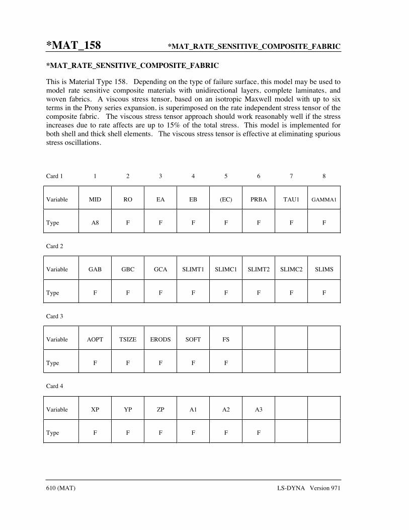
*MAT_158 *MAT_RATE_SENSITIVE_COMPOSITE_FABRIC
610 (MAT) LS-DYNA Version 971
*MAT_RATE_SENSITIVE_COMPOSITE_FABRIC
This is Material Type 158. Depending on the type of failure surface, this model may be used to model rate sensitive composite materials with unidirectional layers, complete laminates, and woven fabrics. A viscous stress tensor, based on an isotropic Maxwell model with up to six terms in the Prony series expansion, is superimposed on the rate independent stress tensor of the composite fabric. The viscous stress tensor approach should work reasonably well if the stress increases due to rate affects are up to 15% of the total stress. This model is implemented for both shell and thick shell elements. The viscous stress tensor is effective at eliminating spurious stress oscillations.
Card 1 1 2 3 4 5 6 7 8
Variable MID RO EA EB (EC) PRBA TAU1 GAMMA1
Type A8 F F F F F F F
Card 2
Variable GAB GBC GCA SLIMT1 SLIMC1 SLIMT2 SLIMC2 SLIMS
Type F F F F F F F F
Card 3
Variable AOPT TSIZE ERODS SOFT FS
Type F F F F F
Card 4
Variable XP YP ZP A1 A2 A3
Type F F F F F F

*MAT_RATE_SENSITIVE_COMPOSITE_FABRIC *MAT_158
LS-DYNA Version 971 611 (MAT)
Card 5 1 2 3 4 5 6 7 8
Variable V1 V2 V3 D1 D2 D3 BETA
Type F F F F F F F
Card 6
Variable E11C E11T E22C E22T GMS
Type F F F F F
Card 7
Variable XC XT YC YT SC
Type F F F F F
Card 8
Variable K
Type F
Card Format for viscoelastic constants. Up to 6 cards may be input. A keyword card (with a “*” in column 1) terminates this input if less than 6 cards are used.
Optional Cards
1 2 3 4 5 6 7 8
Variable GI BETAI
Type F F

*MAT_158 *MAT_RATE_SENSITIVE_COMPOSITE_FABRIC
612 (MAT) LS-DYNA Version 971
VARIABLE DESCRIPTION
MID Material identification. A unique number or label not exceeding 8 characters must be specified.
RO Mass density
EA Ea, Young’s modulus - longitudinal direction
EB Eb, Young’s modulus - transverse direction
(EC) Ec, Young’s modulus - normal direction (not used)
PRBA νba, Poisson’s ratio ba
TAU1 τ1, stress limit of the first slightly nonlinear part of the shear stress versus shear strain curve. The values τ1 and γ1 are used to define a curve of shear stress versus shear strain. These values are input if FS, defined below, is set to a value of -1.
GAMMA1 γ1, strain limit of the first slightly nonlinear part of the shear stress versus shear strain curve.
GAB Gab, shear modulus ab
GBC Gbc, shear modulus bc
GCA Gca, shear modulus ca
SLIMT1 Factor to determine the minimum stress limit after stress maximum (fiber tension).
SLIMC1 Factor to determine the minimum stress limit after stress maximum (fiber compression).
SLIMT2 Factor to determine the minimum stress limit after stress maximum (matrix tension).
SLIMC2 Factor to determine the minimum stress limit after stress maximum (matrix compression).
SLIMS Factor to determine the minimum stress limit after stress maximum (shear).
AOPT Material axes option (see MAT_OPTION TROPIC_ELASTIC for a more complete description):
EQ.0.0: locally orthotropic with material axes determined by element nodes 1, 2, and 4, as with *DEFINE_COORDINATE_ NODES.

*MAT_RATE_SENSITIVE_COMPOSITE_FABRIC *MAT_158
LS-DYNA Version 971 613 (MAT)
VARIABLE DESCRIPTION EQ.2.0: globally orthotropic with material axes determined by
vectors defined below, as with *DEFINE_COORDINATE_ VECTOR.
EQ.3.0: locally orthotropic material axes determined by rotating the material axes about the element normal by an angle (BETA) from a line in the plane of the element defined by the cross product of the vector v with the element normal.
LT.0.0: the absolute value of AOPT is a coordinate system ID number (CID on *DEFINE_COORDINATE_NODES, *DEFINE_ COORDINATE_SYSTEM or *DEFINE_COORDINATE_ VECTOR). Available in R3 version of 971 and later.
TSIZE Time step for automatic element deletion.
ERODS Maximum effective strain for element layer failure. A value of unity would equal 100% strain.
SOFT Softening reduction factor for strength in the crashfront.
FS Failure surface type: EQ.1.0: smooth failure surface with a quadratic criterion for both
the fiber (a) and transverse (b) directions. This option can be used with complete laminates and fabrics.
EQ.0.0: smooth failure surface in the transverse (b) direction with a limiting value in the fiber (a) direction. This model is appropriate for unidirectional (UD) layered composites only.
EQ.-1: faceted failure surface. When the strength values are reached then damage evolves in tension and compression for both the fiber and transverse direction. Shear behavior is also considered. This option can be used with complete laminates and fabrics.
XP YP ZP Define coordinates of point p for AOPT = 1.
A1 A2 A3 Define components of vector a for AOPT = 2.
V1 V2 V3 Define components of vector v for AOPT = 3.
D1 D2 D3 Define components of vector d for AOPT = 2.
BETA Material angle in degrees for AOPT = 3, may be overridden on the element card, see *ELEMENT_SHELL_BETA.
E11C Strain at longitudinal compressive strength, a-axis.
E11T Strain at longitudinal tensile strength, a-axis.

*MAT_158 *MAT_RATE_SENSITIVE_COMPOSITE_FABRIC
614 (MAT) LS-DYNA Version 971
VARIABLE DESCRIPTION
E22C Strain at transverse compressive strength, b-axis.
E22T Strain at transverse tensile strength, b-axis.
GMS Strain at shear strength, ab plane.
XC Longitudinal compressive strength
XT Longitudinal tensile strength, see below.
YC Transverse compressive strength, b-axis, see below.
YT Transverse tensile strength, b-axis, see below.
SC Shear strength, ab plane.
K Optional bulk modulus for the viscoelastic material. If nonzero a Kelvin type behavior will be obtained. Generally, K is set to zero.
GI Optional shear relaxation modulus for the ith term
BETAI Optional shear decay constant for the ith term
Remarks:
See the remark for material type 58, *MAT_LAMINATED_COMPOSITE_FABRIC, for the treatment of the composite material.
Rate effects are taken into account through a Maxwell model using linear viscoelasticity by a convolution integral of the form:
( )0
tkl
ij ijklg t dεσ τ ττ
∂= −∂
where ( )ijkl tg τ− is the relaxation functions for the different stress measures. This stress is added to
the stress tensor determined from the strain energy functional. Since we wish to include only simple rate effects, the relaxation function is represented by six terms from the Prony series:
( )1
m
Nt
mm
g t G e β−
==
We characterize this in the input by the shear moduli, iG , and decay constants, iβ . An
arbitrary number of terms, not exceeding 6, may be used when applying the viscoelastic model. The composite failure is not directly affected by the presence of the viscous stress tensor.

*MAT_CSCM *MAT_159
LS-DYNA Version 971 615 (MAT)
*MAT_CSCM _{OPTION}
This is material type 159. This is a smooth or continuous surface cap model and is available for solid elements in LS-DYNA. The user has the option of inputting his own material properties (<BLANK> option), or requesting default material properties for normal strength concrete (CONCRETE).
Available options include:
<BLANK>
CONCRETE
such that the keyword cards appear as:
*MAT_CSCM*MAT_CSCM _CONCRETE
Define the next two cards for all options:
Card 1 1 2 3 4 5 6 7 8
Variable MID RO NPLOT INCRE IRATE ERODE RECOV ITRETRC
Type A8 F I F I F F I
Card 2
Variable PRED
Type F
Define the following card for the CONCRETE option. Do not define for the <BLANK> option.
Card 3 1 2 3 4 5 6 7 8
Variable FPC DAGG UNITS
Type F F I

*MAT_159 *MAT_CSCM
616 (MAT) LS-DYNA Version 971
Define the following cards for the <BLANK> option. Do not define for CONCRETE.
Card 3 1 2 3 4 5 6 7 8
Variable G K ALPHA THETA LAMDA BETA NH CH
Type F F F F F F F F
Card 4
Variable ALPHA1 THETA1 LAMDA1 BETA1 ALPHA2 THETA2 LAMDA2 BETA2
Type F F F F F F F F
Card 5
Variable R X0 W D1 D2
Type F F F F F
Card 6
Variable B GFC D GFT GFS PWRC PWRT PMOD
Type F F F F F F F F
Card 7
Variable ETA0C NC ETA0T NT OVERC OVERT SRATE REPOW
Type F F F F F F F F

*MAT_CSCM *MAT_159
LS-DYNA Version 971 617 (MAT)
VARIABLE DESCRIPTION
MID Material identification. A unique number or label not exceeding 8 characters must be specified.
RO Mass density.
NPLOT Controls what is written as component 7 to the d3plot database. LS-Prepost always blindly labels this component as effective plastic strain:
EQ.1: Maximum of brittle and ductile damage (default). EQ.2: Maximum of brittle and ductile damage, with recovery of
brittle damage. EQ.3: Brittle damage. EQ.4: Ductile damage. EQ.5: κ (intersection of cap with shear surface). EQ.6: X0 (intersection of cap with pressure axis).
EQ.7: pvε (plastic volume strain).
INCRE Maximum strain increment for subincrementation. If left blank, a default value is set during initialization based upon the shear strength and stiffness.
IRATE Rate effects options: EQ.0: Rate effects model turned off (default). EQ.1: Rate effects model turned on.
ERODE Elements erode when damage exceeds 0.99 and the maximum principal strain exceeds ERODE-1.0. For erosion that is independent of strain, set ERODE equal to 1.0. Erosion does not occur if ERODE is less than 1.0.
RECOV The modulus is recovered in compression when RECOV is equal to 0 (default). The modulus remains at the brittle damage level when RECOV is equal to 1. Partial recovery is modeled for values of RECOV between 0 and 1. Two options are available:
EQ.1: Input a value between 0 and 1. Recovery is based upon the sign of the pressure invariant only.
EQ.2: Input a value between 10 and 11. Recovery is based upon the sign of both the pressure and volumetric strain. In this case, RECOV=RECOV-10, and a flag is set to request the volumetric strain check.
IRETRC Cap retraction option: EQ.0: Cap does not retract (default). EQ.1: Cap retracts.
PRED Pre-existing damage (0 ≤ PreD < 1). If left blank, the default is zero (no pre-existing damage).
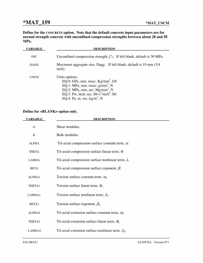
*MAT_159 *MAT_CSCM
618 (MAT) LS-DYNA Version 971
Define for the CONCRETE option. Note that the default concrete input parameters are for normal strength concrete with unconfined compression strengths between about 28 and 58 MPa.
VARIABLE DESCRIPTION
FPC Unconfined compression strength, f 'C. If left blank, default is 30 MPa.
DAGG Maximum aggregate size, Dagg. If left blank, default is 19 mm (3/4 inch).
UNITS Units options: EQ.0: GPa, mm, msec, Kg/mm3, kN EQ.1: MPa, mm, msec, g/mm3, N EQ.2: MPa, mm, sec, Mg/mm3, N EQ.3: Psi, inch, sec, lbf-s2/inch4, lbf EQ.4: Pa, m, sec, kg/m3, N
Define for <BLANK> option only.
VARIABLE DESCRIPTION
G Shear modulus.
K Bulk modulus.
ALPHA Tri-axial compression surface constant term, α.
ΤΗΕΤΑ Tri-axial compression surface linear term, θ.
LAMDA Tri-axial compression surface nonlinear term, λ.
ΒΕΤΑ Tri-axial compression surface exponent, β.
ALPHA1 Torsion surface constant term, α1.
ΤΗΕΤΑ1 Torsion surface linear term, θ1.
LAMDA1 Torsion surface nonlinear term, λ1.
ΒΕΤΑ1 Torsion surface exponent, β1.
ALPHA2 Tri-axial extension surface constant term, α2.
ΤΗΕΤΑ2 Tri-axial extension surface linear term, θ2.
LAMDA2 Tri-axial extension surface nonlinear term, λ2.

*MAT_CSCM *MAT_159
LS-DYNA Version 971 619 (MAT)
VARIABLE DESCRIPTION
ΒΕΤΑ2 Tri-axial extension surface exponent, β2.
NH Hardening initiation, NH.
CH Hardening rate, CH.
R Cap aspect ratio, R.
X0 Cap initial location, X0.
W Maximum plastic volume compaction, W.
D1 Linear shape parameter, D1.
D2 Quadratic shape parameter, D2.
B Ductile shape softening parameter, B.
GFC Fracture energy in uniaxial stress Gfc.
D Brittle shape softening parameter, D.
GFT Fracture energy in uniaxial tension, Gft.
GFS Fracture energy in pure shear stress, Gfs.
PWRC Shear-to-compression transition parameter.
PWRT Shear-to-tension transition parameter.
PMOD Modify moderate pressure softening parameter.
ETA0C Rate effects parameter for uniaxial compressive stress, η0c.
NC Rate effects power for uniaxial compressive stress, NC.
ETA0T Rate effects parameter for uniaxial tensile stress, η0t.
NT Rate effects power for uniaxial tensile stress, Nt.
OVERC Maximum overstress allowed in compression.
OVERT Maximum overstress allowed in tension.
SRATE Ratio of effective shear stress to tensile stress fluidity parameters.
REPOW Power which increases fracture energy with rate effects.

*MAT_159 *MAT_CSCM
620 (MAT) LS-DYNA Version 971
Remarks:
Model Formulation and Input Parameters This is a cap model with a smooth intersection between the shear yield surface and
hardening cap, as shown in Figure 159.1. The initial damage surface coincides with the yield surface. Rate effects are modeled with viscoplasticity. For a complete theoretical description, with references and example problems see [Murray 2007] and [Murray, Abu-Odeh and Bligh 2007].
Figure 159.1. General shape of the concrete model yield surface in two-dimensions.
Stress Invariants. The yield surface is formulated in terms of three stress invariants: J1 is the first invariant of the stress tensor, 2J ′ is the second invariant of the deviatoric stress tensor, and
3J ′ is the third invariant of the deviatoric stress tensor. The invariants are defined in terms of
the deviatoric stress tensor, Sij and pressure, P, as follows:
kijkij3
ijij2
1
SSSJ
SSJ
PJ
3
12
1
3
=′
=′
=
Plasticity Surface. The three invariant yield function is based on these three invariants, and the cap hardening parameter, κ, as follows:
cf1 FFJJ,Jf(J 22232 ),, ℜ−′=′′ κ

*MAT_CSCM *MAT_159
LS-DYNA Version 971 621 (MAT)
Here Ff is the shear failure surface, Fc is the hardening cap, and ℜ is the Rubin three-invariant
reduction factor. The cap hardening parameter κ is the value of the pressure invariant at the intersection of the cap and shear surfaces.
Trial elastic stress invariants are temporarily updated via the trial elastic stress tensor, σT. These are denoted J1
T, J2′T, and J3′T. Elastic stress states are modeled when f (J1T,J2′T,J3′T,κΤ ) ≤ 0.
Elastic-plastic stress states are modeled when f (J1T,J2′T,J3′T,κΤ ) > 0. In this case, the plasticity
algorithm returns the stress state to the yield surface such that f (J1P,J2′P,J3′P,κP ) = 0. This is
accomplished by enforcing the plastic consistency condition with associated flow.
Shear Failure Surface. The strength of concrete is modeled by the shear surface in the tensile and low confining pressure regimes:
111exp)( JJF J
f θλα β +−= −
Here the values of θλβα and,,, are selected by fitting the model surface to strength measurements from triaxial compression (TXC) tests conducted on plain concrete cylinders.
Rubin Scaling Function. Concrete fails at lower values of '2J3 (principal stress difference) for
triaxial extension (TXE) and torsion (TOR) tests than it does for TXC tests conducted at the same pressure. The Rubin scaling function ℜ determines the strength of concrete for any state of stress relative to the strength for TXC, via ℜFf. Strength in torsion is modeled as Q1Ff . Strength in TXE is modeled as Q2Ff, where:
12222
11111
12
11
JexpQ
JexpQ
J
J
θλα
θλαβ
β
+−=
+−=−
−
Cap Hardening Surface. The strength of concrete is modeled by a combination of the cap and shear surfaces in the low to high confining pressure regimes. The cap is used to model plastic volume change related to pore collapse (although the pores are not explicitly modeled). The isotropic hardening cap is a two-part function that is either unity or an ellipse:
[ ] [ ][ ] 2
1111
)()(2
)()()(1),
κκ
κκκκ
LX
LJLJLJJ(Fc
−
−+−−−=
where L(κ) is defined as:
>=
otherwise
ifL
0
0)(κ
κκκκ

*MAT_159 *MAT_CSCM
622 (MAT) LS-DYNA Version 971
The equation for Fc is equal to unity for J1 ≤ L(κ). It describes the ellipse for J1 > L(κ). The intersection of the shear surface and the cap is at J1 = κ. κ0 is the value of J1 at the initialintersection of the cap and shear surfaces before hardening is engaged (before the cap moves). The equation for L(κ) restrains the cap from retracting past its initial location at κ0.
The intersection of the cap with the J1 axis is at J1 = X(κ). This intersection depends upon the cap ellipticity ratio R, where R is the ratio of its major to minor axes:
))(()()( κκκ LRFLX f+=
The cap moves to simulate plastic volume change. The cap expands (X(κ) and κ increase) to simulate plastic volume compaction. The cap contracts (X(κ) and κ decrease) to simulate plastic volume expansion, called dilation. The motion (expansion and contraction) of the cap is based upon the hardening rule:
( ) ( )( )21 0 2 01 exp D X X D X Xp
v Wε − − − −= −
Here pvε the plastic volume strain, W is the maximum plastic volume strain, and D1 and D2 are
model input parameters. X0 is the initial location of the cap when κ=κ0.
The five input parameters (X0, W, D1, D2, and R) are obtained from fits to the pressure-volumetric strain curves in isotropic compression and uniaxial strain. X0 determines the pressure at which compaction initiates in isotropic compression. R, combined with X0, determines the pressure at which compaction initiates in uniaxial strain. D1, and D2 determine the shape of the pressure-volumetric strain curves. W determines the maximum plastic volume compaction.
Shear Hardening Surface. In unconfined compression, the stress-strain behavior of concrete exhibits nonlinearity and dilation prior to the peak. Such behavior is be modeled with an initial shear yield surface, NHFf , which hardens until it coincides with the ultimate shear yield surface, Ff. Two input parameters are required. One parameter, NH, initiates hardening by setting the location of the initial yield surface. A second parameter, CH, determines the rate of hardening (amount of nonlinearity).
Damage. Concrete exhibits softening in the tensile and low to moderate compressive regimes.
vpij
dij d σσ )1( −=
A scalar damage parameter, d, transforms the viscoplastic stress tensor without damage, denoted σvp, into the stress tensor with damage, denoted σd. Damage accumulation is based upon two distinct formulations, which we call brittle damage and ductile damage. The initial damage threshold is coincident with the shear plasticity surface, so the threshold does not have to be specified by the user.

*MAT_CSCM *MAT_159
LS-DYNA Version 971 623 (MAT)
Ductile Damage. Ductile damage accumulates when the pressure (P) is compressive and an energy-type term, τc, exceeds the damage threshold, τ0c. Ductile damage accumulation depends upon the total strain components, εij, as follows:
c
1
2 ij ijτ σ ε=
The stress components σij are the elasto-plastic stresses (with kinematic hardening) calculated before application of damage and rate effects.
Brittle Damage. Brittle damage accumulates when the pressure is tensile and an energy-type term, τt, exceeds the damage threshold, τ0t. Brittle damage accumulation depends upon the maximum principal strain, ε max, as follows:
2maxt ετ E=
Softening Function. As damage accumulates, the damage parameter d increases from an initial value of zero, towards a maximum value of one, via the following formulations:
Brittle Damage −−+
+=−
1(
expD1
D1
D9990)(
)t0tCt τττ .d
Ductile Damage −−+
+=−
1(A
expB1
B1
B)(
)0cc
maxc
dd τττ
The damage parameter that is applied to the six stresses is equal to the current maximum of the brittle or ductile damage parameter. The parameters A and B or C and D set the shape of the softening curve plotted as stress-displacement or stress-strain. The parameter dmax is the maximum damage level that can be attained. It is calculated internally calculated and is less than one at moderate confining pressures. The compressive softening parameter, A, may also be reduced with confinement, using the input parameter pmod, as follows:
pmodmaxd )001.0A(A +=
Regulating Mesh Size Sensitivity. The concrete model maintains constant fracture energy, regardless of element size. The fracture energy is defined here as the area under the stress-displacement curve from peak strength to zero strength. This is done by internally formulating the softening parameters A and C in terms of the element length, l (cube root of the element volume), the fracture energy, Gf, the initial damage threshold, τ0t or τ0c, and the softening shape parameters, D or B.
The fracture energy is calculated from up to five user-specified input parameters (Gfc, Gft, Gfs,pwrc, pwrc). The user specifies three distinct fracture energy values. These are the fracture energy in uniaxial tensile stress, Gft, pure shear stress, Gfs, and uniaxial compressive stress, Gfc.

*MAT_159 *MAT_CSCM
624 (MAT) LS-DYNA Version 971
The model internally selects the fracture energy from equations which interpolate between the three fracture energy values as a function of the stress state (expressed via two stress invariants). The interpolation equations depend upon the user-specified input powers pwrc and pwrt, as follows.
pwrc
fsfcfsf
pwrt
fsftfsf
J3
Jtrans whereGGtransGGecompressivispressuretheif
J3
J-trans whereGGtransGGtensileispressuretheif
′=−+=
′=−+=
2
1
2
1
)(
)(
The internal parameter trans is limited to range between 0 and 1.
Element Erosion. An element losses all strength and stiffness as d→1. To prevent computational difficulties with very low stiffness, element erosion is available as a user option. An element erodes when d > 0.99 and the maximum principal strain is greater than a user supplied input value, ERODE-1.0.
Viscoplastic Rate Effects. At each time step, the viscoplastic algorithm interpolates between the
elastic trial stress, Tjiσ , and the inviscid stress (without rate effects), p
jiσ , to set the viscoplastic
stress (with rate effects), vpjiσ :
pij
Tij
vpij γγ +−= )1( with
ηηγ/t1
/t
Δ+Δ=
This interpolation depends upon the effective fluidity coefficient, η, and the time step, Δt. The effective fluidity coefficient is internally calculated from five user-supplied input parameters and interpolation equations:
tratesNc
cNt
t
pwrc
scs
pwrt
sts
S
J3
Jtranstransecompressivispressuretheif
J3
J-transtranstensileispressuretheif
ctηη
εηη
εηη
ηηηη
ηηηη
===
′=−+=
′=−+=
00
2
1
2
1
)(
)(
The input parameters are η0t and Nt for fitting uniaxial tensile stress data, η0c and Nc for fitting the uniaxial compressive stress data, and Srate for fitting shear stress data. The effective strain rate is ε .
This viscoplastic model may predict substantial rate effects at high strain rates (ε >100). To limit rate effects at high strain rates, the user may input overstress limits in tension (overt) and

*MAT_CSCM *MAT_159
LS-DYNA Version 971 625 (MAT)
compression (overc). These input parameters limit calculation of the fluidity parameter, as follows:
if E >ηε over then η = ε
over
where over = overt when the pressure is tensile, and over = overc when the pressure is compressive.
The user has the option of increasing the fracture energy as a function of effective strain rate via the repow input parameter, as follows:
repow
fratef f
E1GG
′+=
Here ratefG is the fracture energy enhanced by rate effects, and f ′ is the yield strength before
application of rate effects (which is calculated internally by the model). The term in brackets is greater than, or equal to one, and is the approximate ratio of the dynamic to static strength.

*MAT_161, MAT_162 *MAT_COMPOSITE_MSC
626 (MAT) LS-DYNA Version 971
*MAT_COMPOSITE_MSC_{OPTION}
Available options include:
<BLANK>
DMG
These are Material Types 161 and 162. These models may be used to model the progressive failure analysis for composite materials consisting of unidirectional and woven fabric layers. The progressive layer failure criteria have been established by adopting the methodology developed by Hashin [1980] with a generalization to include the effect of highly constrained pressure on composite failure. These failure models can be used to effectively simulate fiber failure, matrix damage, and delamination behavior under all conditions - opening, closure, and sliding of failure surfaces. The model with DMG option (material 162) is a generalization of the basic layer failure model of Material 161 by adopting the damage mechanics approach for characterizing the softening behavior after damage initiation. These models require an additional license from Materials Sciences Corporation, which developed and supports these models.
Card 1 1 2 3 4 5 6 7 8
Variable MID RO EA EB EC PRBA PRCA PRCB
Type A8 F F F F F F F
Card 2
Variable GAB GBC GCA AOPT MACF
Type F F F F I
Card 3
Variable XP YP ZP A1 A2 A3
Type F F F F F F

*MAT_COMPOSITE_MSC *MAT_161, MAT_162
LS-DYNA Version 971 627 (MAT)
Card 4 1 2 3 4 5 6 7 8
Variable V1 V2 V3 D1 D2 D3 BETA
Type F F F F F F F
Card 5
Variable SAT SAC SBT SBC SCT SFC SFS SAB
Type F F F F F F F F
Card 6
Variable SBC SCA SFFC AMODEL PHIC E_LIMT S_DELM
Type F F F F F F F
Card 7
Variable OMGMX ECRSH EEXPN CERATE1 AM1
Type F F F F F
Define the following cards if and only if the option DMG is specified
Card 8 1 2 3 4 5 6 7 8
Variable AM2 AM3 AM4 CERATE2 CERATE3 CERATE4
Type F F F F F F

*MAT_161, MAT_162 *MAT_COMPOSITE_MSC
628 (MAT) LS-DYNA Version 971
VARIABLE DESCRIPTION
MID Material identification. A unique number or label not exceeding 8 characters must be specified.
RO Mass density
EA Ea, Young’s modulus - longitudinal direction
EB Eb, Young’s modulus - transverse direction
EC Ec, Young’s modulus - through thickness direction
PRBA νba, Poisson’s ratio ba
PRCA νca, Poisson’s ratio ca
PRCB νcb, Poisson’s ratio cb
GAB Gab, shear modulus ab
GBC Gbc, shear modulus bc
GCA Gca, shear modulus ca
AOPT Material axes option, see Figure 2.1: EQ.0.0: locally orthotropic with material axes determined by
element nodes as shown in Figure 2.1. Nodes 1, 2, and 4 of an element are identical to the Nodes used for the definition of a coordinate system by *DEFINE_COORDINATE_NODES.
EQ.1.0: locally orthotropic with material axes determined by a point in space and the global location of the element center, to define the a-direction.
EQ.2.0: globally orthotropic with material axes determined by vectors defined below, as with *DEFINE_COORDINATE_ VECTOR.
LT.0.0: the absolute value of AOPT is a coordinate system ID number (CID on *DEFINE_COORDINATE_NODES, *DEFINE_ COORDINATE_SYSTEM or *DEFINE_COORDINATE_ VECTOR). Available in R3 version of 971 and later.
MACF Material axes change flag: EQ.1: No change, default, EQ.2: switch material axes a and b, EQ.3: switch material axes a and c, EQ.4: switch material axes b and c.
XP YP ZP Define coordinates of point p for AOPT = 1.

*MAT_COMPOSITE_MSC *MAT_161, MAT_162
LS-DYNA Version 971 629 (MAT)
VARIABLE DESCRIPTION
A1 A2 A3 Define components of vector a for AOPT = 2.
V1 V2 V3 Define components of vector v for AOPT = 3.
D1 D2 D3 Define components of vector d for AOPT = 2.
BETA Layer in-plane rotational angle in degrees.
SAT Longitudinal tensile strength
SAC Longitudinal compressive strength
SBT Transverse tensile strength
SBC Transverse compressive strength
SCT Through thickness tensile strength
SFC Crush strength
SFS Fiber mode shear strength
SAB Matrix mode shear strength, ab plane, see below.
SBC Matrix mode shear strength, bc plane, see below.
SCA Matrix mode shear strength, ca plane, see below.
SFFC Scale factor for residual compressive strength
AMODEL Material models: EQ.1: Unidirectional layer model
EQ.2: Fabric layer model
PHIC Coulomb friction angle for matrix and delamination failure, <90
E_LIMT Element eroding axial strain
S_DELM Scale factor for delamination criterion
OMGMX Limit damage parameter for elastic modulus reduction
ECRSH Limit compressive volume strain for element eroding
EEXPN Limit tensile volume strain for element eroding
CERATE1 Coefficient for strain rate dependent strength properties

*MAT_161, MAT_162 *MAT_COMPOSITE_MSC
630 (MAT) LS-DYNA Version 971
VARIABLE DESCRIPTION
AM1 Coefficient for strain rate softening property for fiber damage in a direction.
AM2 Coefficient for strain rate softening property for fiber damage in b direction.
AM3 Coefficient for strain rate softening property for fiber crush and punch shear damage.
AM4 Coefficient for strain rate softening property for matrix and delamination damage.
CERATE2 Coefficient for strain rate dependent axial moduli.
CERATE3 Coefficient for strain rate dependent shear moduli.
CERATE4 Coefficient for strain rate dependent transverse moduli.
Material Models:
The unidirectional and fabric layer failure criteria and the associated property degradation models for material 161 are described as follows. All the failure criteria are expressed in terms of stress components based on ply level stresses (σa ,σ b,σc ,τab ,τbc ,τ ca ) and the associated elastic moduli are (Ea, Eb ,Ec,Gab ,Gbc, Gca ). Note that for the unidirectional model, a, b and c denote the fiber, in-plane transverse and out-of-plane directions, respectively, while for the fabric model, a, b and c denote the in-plane fill, in-plane warp and out-of-plane directions, respectively.
Unidirectional lamina model Three criteria are used for fiber failure, one in tension/shear, one in compression and another one in crush under pressure. They are chosen in terms of quadratic stress forms as follows:
Tensile/shear fiber mode:
2 2 2
1 21 0a ab ca
aT FS
fS S
σ τ τ+= + − =
Compression fiber mode:
2''
2 1 0,2
b caa a
aC
fS
σ σσ σ σ+
= − = = − + −
Crush mode:

*MAT_COMPOSITE_MSC *MAT_161, MAT_162
LS-DYNA Version 971 631 (MAT)
2
3 1 0,3
a b c
FC
pf p
S
σ σ σ+ += − = = −
where are Macaulay brackets, aTS and SaC are the tensile and compressive strengths in the
fiber direction, and SFS and SFC are the layer strengths associated with the fiber shear and crush failure, respectively.
Matrix mode failures must occur without fiber failure, and hence they will be on planes parallel to fibers. For simplicity, only two failure planes are considered: one is perpendicular to the planes of layering and the other one is parallel to them. The matrix failure criteria for the failure plane perpendicular and parallel to the layering planes, respectively, have the forms:
Perpendicular matrix mode:
2 2 2
4 '1 0b bc ab
bT bc ab
fS S S
σ τ τ= + + − =
Parallel matrix mode (Delamination):
2 2 2
25 " 1 0c bc ca
bT bc ca
f SS S S
σ τ τ= + + − =
where SbT is the transverse tensile strength. Based on the Coulomb-Mohr theory, the shear strengths for the transverse shear failure and the two axial shear failure modes are assumed to be the forms,
(0) tan( )ab ab bS S ϕ σ= + −
' (0) tan( )bc bc bS S ϕ σ= + −
(0) tan( )ca ca cS S ϕ σ= + −
" (0) tan( )bc bc cS S ϕ σ= + −
where ϕ is a material constant as tan( )ϕ is similar to the coefficient of friction, and Sab(0) , Sca
(0) and
Sbc(0) are the shear strength values of the corresponding tensile modes.
Failure predicted by the criterion of f4 can be referred to as transverse matrix failure, while the matrix failure predicted by f5, which is parallel to the layer, can be referred as the delamination mode when it occurs within the elements that are adjacent to the ply interface. Note that a scale factor S is introduced to provide better correlation of delamination area with experiments. The scale factor S can be determined by fitting the analytical prediction to experimental data for the delamination area.

*MAT_161, MAT_162 *MAT_COMPOSITE_MSC
632 (MAT) LS-DYNA Version 971
When fiber failure in tension/shear mode is predicted in a layer by f1, the load carrying capacity of that layer is completely eliminated. All the stress components are reduced to zero instantaneously (100 time steps to avoid numerical instability). For compressive fiber failure, the layer is assumed to carry a residual axial load, while the transverse load carrying capacity is reduced to zero. When the fiber compressive failure mode is reached due to f2, the axial layer
compressive strength stress is assumed to reduce to a residual value SRC (= * ACSFFC S ). The
axial stress is then assumed to remain constant, i.e., a RCSσ = − , for continuous compressive
loading, while the subsequent unloading curve follows a reduced axial modulus to zero axial stress and strain state. When the fiber crush failure occurs, the material is assumed to behave elastically for compressive pressure, p > 0, and to carry no load for tensile pressure, p < 0.
When a matrix failure (delamination) in the a-b plane is predicted, the strength values for Sca
(0) and Sbc(0) are set to zero. This results in reducing the stress components cσ , bcτ and caτ to the
fractured material strength surface. For tensile mode, 0cσ > , these stress components are
reduced to zero. For compressive mode, 0cσ < , the normal stress cσ is assumed to deform
elastically for the closed matrix crack. Loading on the failure envelop, the shear stresses are assumed to ‘slide’ on the fractured strength surface (frictional shear stresses) like in an ideal plastic material, while the subsequent unloading shear stress-strain path follows reduced shear moduli to the zero shear stress and strain state for both bcτ and caτ components.
The post failure behavior for the matrix crack in the a-c plane due to f4 is modeled in the same fashion as that in the a-b plane as described above. In this case, when failure occurs, Sab
(0) and Sbc(0) are reduced to zero instantaneously. The post fracture response is then governed by
failure criterion of f5 with Sab(0) = 0 and ( )0
bcS = 0. For tensile mode, 0bσ > , bσ , abτ and bcτ are
zero. For compressive mode, 0bσ < , bσ is assumed to be elastic, while abτ and bcτ ‘slide’ on
the fracture strength surface as in an ideal plastic material, and the unloading path follows reduced shear moduli to the zero shear stress and strain state. It should be noted that bcτ is
governed by both the failure functions and should lie within or on each of these two strength surfaces.
Fabric lamina model The fiber failure criteria of Hashin for a unidirectional layer are generalized to characterize the fiber damage in terms of strain components for a plain weave layer. The fill and warp fiber tensile/shear failure are given by the quadratic interaction between the associated axial and shear stresses, i.e.
( )2 2 2
6 21 0
ab caa
aT aFS
fS S
τ τσ += + − =
( )2 2 2
7 21 0
ab bcb
bT bFS
fS S
τ τσ += + − =

*MAT_COMPOSITE_MSC *MAT_161, MAT_162
LS-DYNA Version 971 633 (MAT)
where SaT and SbT are the axial tensile strengths in the fill and warp directions, respectively, and SaFS and SbFS are the layer shear strengths due to fiber shear failure in the fill and warp directions. These failure criteria are applicable when the associated σa or σb is positive. It is assumed SaFS = SFS, and
* /bFS bT aTS SFS S S= .
When σa or σb is compressive, it is assumed that the in-plane compressive failure in both the fill and warp directions are given by the maximum stress criterion, i.e.
2'
'8 1 0,
a
a a caC
fS
σσ σ σ= − = = − + −
2'
'9 1 0,
b
b b cbC
fS
σσ σ σ= − = = − + −
where SaC and SbC are the axial compressive strengths in the fill and warp directions, respectively. The crush failure under compressive pressure is
2
10 1 0,3
a b c
FC
pf p
S
σ σ σ+ += − = = −
A plain weave layer can fail under in-plane shear stress without the occurrence of fiber breakage. This in-plane matrix failure mode is given by
2
11 1 0ab
ab
fS
τ= − =
where Sab is the layer shear strength due to matrix shear failure.
Another failure mode, which is due to the quadratic interaction between the thickness stresses, is expected to be mainly a matrix failure. This through the thickness matrix failure criterion is
2 2 2
212 1 0c bc ca
cT bc ca
f SS S S
σ τ τ= + + − =
where ScT is the through the thickness tensile strength, and Sbc , and Sca are the shear strengths
assumed to depend on the compressive normal stress σ c , i.e.,

*MAT_161, MAT_162 *MAT_COMPOSITE_MSC
634 (MAT) LS-DYNA Version 971
(0)
(0)tan( )ca ca
cbc bc
S S
S Sϕ σ= + −
When failure predicted by this criterion occurs within elements that are adjacent to the ply interface, the failure plane is expected to be parallel to the layering planes, and, thus, can be referred to as the delamination mode. Note that a scale factor S is introduced to provide better correlation of delamination area with experiments. The scale factor S can be determined by fitting the analytical prediction to experimental data for the delamination area.
Similar to the unidirectional model, when fiber tensile/shear failure is predicted in a layer by f6 or f7, the load carrying capacity of that layer in the associated direction is completely eliminated. For compressive fiber failure due to by f8 or f9, the layer is assumed to carry a residual axial load in the failed direction, while the load carrying capacity transverse to the failed direction is assumed unchanged. When the compressive axial stress in a layer reaches the compressive axial strength SaC or SbC , the axial layer stress is assumed to be reduced to the residual strength SaRC or SbRC where SaRC = SFFC* SaC and SbRC = SFFC* SbC . The axial stress is assumed to remain constant, i.e., σa = − SaCR or σb = − SbCR , for continuous compressive loading, while the subsequent unloading curve follows a reduced axial modulus. When the fiber crush failure is occurred, the material is assumed to behave elastically for compressive pressure, p > 0, and to carry no load for tensile pressure, p < 0.
When the in-plane matrix shear failure is predicted by f11 the axial load carrying capacity within a failed element is assumed unchanged, while the in-plane shear stress is assumed to be reduced to zero.
For through the thickness matrix (delamination) failure given by equations f12, the in-plane load carrying capacity within the element is assumed to be elastic, while the strength values for the tensile mode, Sca
(0) and Sbc(0) , are set to zero. For tensile mode, 0cσ > , the through
the thickness stress components are reduced to zero. For compressive mode, 0cσ < , cσ is
assumed to be elastic, while bcτ and caτ ‘slide’ on the fracture strength surface as in an ideal
plastic material, and the unloading path follows reduced shear moduli to the zero shear stress and strain state.
The effect of strain-rate on the layer strength values of the fiber failure modes is modeled by the strain-rate dependent functions for the strength values { }RTS as
{ }0 1
0
{ } { } 1 lnRT rateS S Cεε
= +
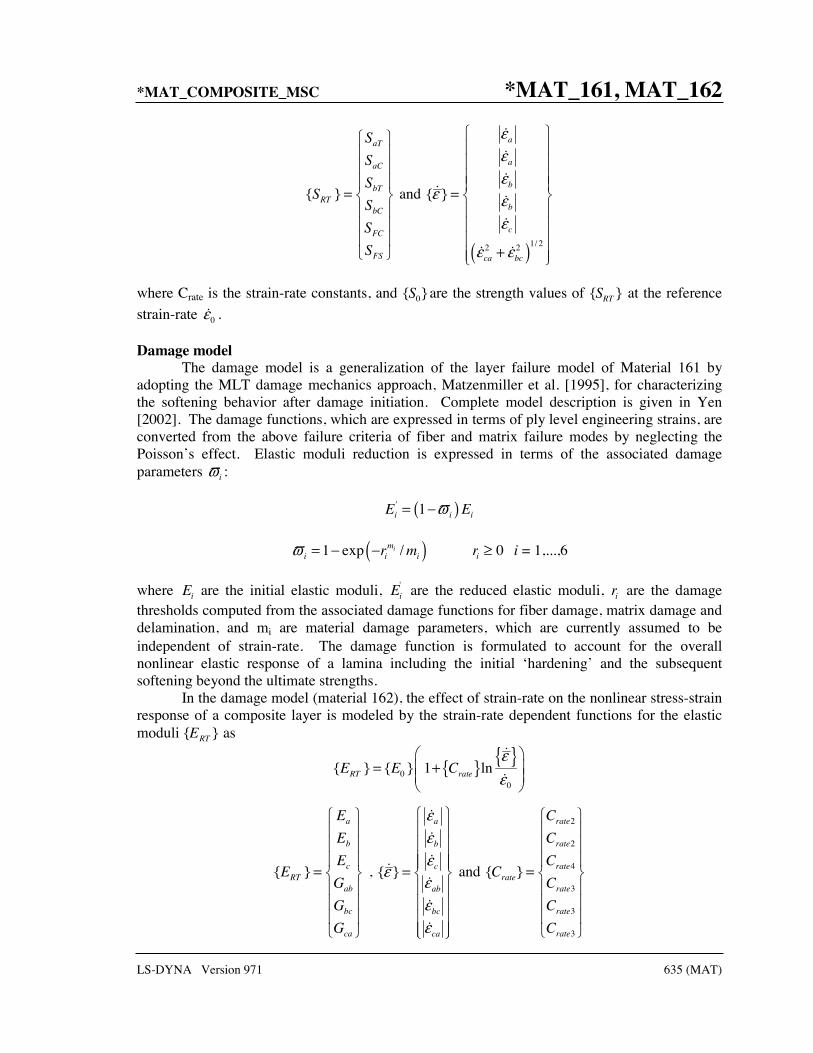
*MAT_COMPOSITE_MSC *MAT_161, MAT_162
LS-DYNA Version 971 635 (MAT)
{ }
aT
aC
bTRT
bC
FC
FS
S
S
SS
S
S
S
= and
( )1/ 22 2
{ }
a
a
b
b
c
ca bc
εεε
ε εε
ε ε
=
+
where Crate is the strain-rate constants, and {S0}are the strength values of {SRT } at the reference
strain-rate 0ε .
Damage model The damage model is a generalization of the layer failure model of Material 161 by adopting the MLT damage mechanics approach, Matzenmiller et al. [1995], for characterizing the softening behavior after damage initiation. Complete model description is given in Yen [2002]. The damage functions, which are expressed in terms of ply level engineering strains, are converted from the above failure criteria of fiber and matrix failure modes by neglecting the Poisson’s effect. Elastic moduli reduction is expressed in terms of the associated damage parameters ϖi :
( )' 1i i iE Eϖ= −
( )1 exp /imi i ir mϖ = − − ri ≥ 0 i = 1,...,6
where Ei are the initial elastic moduli, Ei' are the reduced elastic moduli, ri are the damage
thresholds computed from the associated damage functions for fiber damage, matrix damage and delamination, and mi are material damage parameters, which are currently assumed to be independent of strain-rate. The damage function is formulated to account for the overall nonlinear elastic response of a lamina including the initial ‘hardening’ and the subsequent softening beyond the ultimate strengths. In the damage model (material 162), the effect of strain-rate on the nonlinear stress-strain response of a composite layer is modeled by the strain-rate dependent functions for the elastic moduli {ERT } as
{ } { }0
0
{ } { } 1 lnRT rateE E Cεε
= +
{ }
a
b
cRT
ab
bc
ca
E
E
EE
G
G
G
= , { }
a
b
c
ab
bc
ca
εεε
εεεε
= and
2
2
4
3
3
3
{ }
rate
rate
raterate
rate
rate
rate
C
C
CC
C
C
C
=

*MAT_161, MAT_162 *MAT_COMPOSITE_MSC
636 (MAT) LS-DYNA Version 971
where {Crate} are the strain-rate constants. {E0 } are the modulus values of {ERT } at the reference
strain-rate 0ε .
Element Erosion:
A failed element is eroded in any of three different ways:
1. If fiber tensile failure in a unidirectional layer is predicted in the element and the axial tensile strain is greater than E_LIMT. For a fabric layer, both in-plane directions are failed and exceed E_LIMT.
2. If compressive relative volume in a failed element is smaller than ECRSH.
3. If tensile relative volume in a failed element is greater than EEXPN.
Damage History Parameters:
Information about the damage history variables for the associated failure modes can be plotted in LS-PrePost. These additional history variables are tabulated below:
History Variable
Description Value LS-PrePost
History Variable 1. efa(I) Fiber mode in a 7 2. efb(I) Fiber mode in b 0-elastic 8 3. efp(I) Fiber crush mode 9
4. em(I) Perpendicular matrix mode
≥ 1-failed 10
5. ed(I) Parallel matrix/
delamination mode 11
6. delm(I) delamination mode 12

*MAT_MODIFIED_CRUSHABLE_FOAM *MAT_163
LS-DYNA Version 971 637 (MAT)
*MAT_MODIFIED_CRUSHABLE_FOAM
This is Material Type 163 which is dedicated to modeling crushable foam with optional damping, tension cutoff, and strain rate effects. Unloading is fully elastic. Tension is treated as elastic-perfectly-plastic at the tension cut-off value.
Card 1 1 2 3 4 5 6 7 8
Variable MID RO E PR TID TSC DAMP NCYCLE
Type A8 F F F F F F F
Default none none none none none 0.0 0.10 12.
Card 2
Variable SRCLMT
Type F
Default 1.E+20
VARIABLE DESCRIPTION
MID Material identification. A unique number or label not exceeding 8 characters must be specified.
RO Mass density
E Young’s modulus
PR Poisson’s ratio
TID Table ID defining yield stress versus volumetric strain, γ, at different strain rates.
TSC Tensile stress cutoff. A nonzero, positive value is strongly recommended for realistic behavior.
DAMP Rate sensitivity via damping coefficient (.05<recommended value<.50).
NCYCLE Number of cycles to determine the average volumetric strain rate.
SRCLMT Strain rate change limit.

*MAT_163 *MAT_MODIFIED_CRUSHABLE_FOAM
638 (MAT) LS-DYNA Version 971
Remarks:
The volumetric strain is defined in terms of the relative volume, V, as:
γ = 1.-V
The relative volume is defined as the ratio of the current to the initial volume. In place of the effective plastic strain in the D3PLOT database, the integrated volumetric strain is output.
This material is an extension of material 63, *MAT_CRUSHABLE_FOAM. It allows the yield stress to be a function of both volumetric strain rate and volumetric strain. Rate effects are accounted for by defining a table of curves using *DEFINE_TABLE. Each curve defines the yield stress versus volumetric strain for a different strain rate. The yield stress is obtained by interpolating between the two curves that bound the strain rate.
To prevent high frequency oscillations in the strain rate from causing similar high frequency oscillations in the yield stress, a modified volumetric strain rate is used when interpolating to obtain the yield stress. The modified strain rate is obtained as follows. If NYCLE is >1, then the modified strain rate is obtained by a time average of the actual strain rate over NCYCLE solution cycles. For SRCLMT>0, the modified strain rate is capped so that during each cycle, the modified strain rate is not permitted to change more than SRCLMT multiplied by the solution time step.
Figure 163.1. Rate effects are defined by a family of curves giving yield stress versus volumetric strain where V is the relative volume.

*MAT_BRAIN_LINEAR_VISCOELASTIC *MAT_164
LS-DYNA Version 971 639 (MAT)
*MAT_BRAIN_LINEAR_VISCOELASTIC
This is Material Type 164. This material is a Kelvin-Maxwell model for modeling brain tissue, which is valid for solid elements only. See Remarks below.
Card 1 1 2 3 4 5 6 7 8
Variable MID RO BULK G0 GI DC FO SO
Type A8 F F F F F F F
Default none none none none none 0.0 0.0 0.0
VARIABLE DESCRIPTION
MID Material identification. A unique number or label not exceeding 8 characters must be specified.
RO Mass density
BULK Bulk modulus (elastic)
G0 Short-time shear modulus, G0
GI Long-time (infinite) shear modulus, G
DC Maxwell decay constant, β[FO=0.0] or Kelvin relaxation constant, τ [FO=1.0]
FO Formulation option: EQ.0.0: Maxwell, EQ.1.0: Kelvin.
SO Strain (logarithmic) output option to control what is written as component 7 to the d3plot database. (LS-Prepost always blindly labels this component as effective plastic strain.) The maximum values are updated for each element each time step:
EQ.0.0: maximum principal strain that occurs during the calculation,
EQ.1.0: maximum magnitude of the principal strain values that occurs during the calculation,
EQ.2.0: maximum effective strain that occurs during the calculation.

*MAT_164 *MAT_BRAIN_LINEAR_VISCOELASTIC
640 (MAT) LS-DYNA Version 971
Remarks:
The shear relaxation behavior is described for the Maxwell model by:
0( ) ( ) tG t G G G e β−− ∞= +
A Jaumann rate formulation is used
( ) ( )0
2t
ij ijG t D dtσ τ τ∇′ ′= −
where the prime denotes the deviatoric part of the stress rate, σ∇
ij , and the strain rate Dij . For the Kelvin model the stress evolution equation is defined as:
( ) ( )0
11 1ij ij ijij ij ij
Gs s G e eδ δ
τ τ∞+ = + + +
The strain data as written to the d3plot database may be used to predict damage, see [Bandak 1991].

*MAT_PLASTIC_NONLINEAR_KINEMATIC *MAT_165
LS-DYNA Version 971 641 (MAT)
*MAT_PLASTIC_NONLINEAR_KINEMATIC
This is Material Type 165. This relatively simple model, based on a material model by Lemaitre and Chaboche [1990], is suited to model nonlinear kinematic hardening plasticity. The model accounts for the nonlinear Bauschinger effect, cyclic hardening, and ratcheting. Huang [2006] programmed this model and provided it as a user subroutine. It is a very cost effective model and is available shell and solid elements. This material model is available starting with the R3 release of Version 971.
Card 1 1 2 3 4 5 6 7 8
Variable MID RO E PR SIGY H C GAMMA
Type A8 F F F F F F F
Default none none none none none 0.0 0.0 0.0
Card 2
Variable FS
Type F
Default 1.E+16
VARIABLE DESCRIPTION
MID Material identification. A unique number or label not exceeding 8 characters must be specified.
RO Mass density.
E Young’s modulus.
PR Poisson’s ratio.
SIGY Initial yield stress, 0yσ .
H Isotropic plastic hardening modulus
C Kinematic hardening modulus

*MAT_165 *MAT_PLASTIC_NONLINEAR_KINEMATIC
642 (MAT) LS-DYNA Version 971
VARIABLE DESCRIPTION
GAMMA Kinematic hardening parameter, γ .
FS Failure strain for eroding elements.
Remarks:
If the isotropic hardening modulus, H, is nonzero, the size of the surface increases as function of the equivalent plastic strain, pε :
0p
y y Hσ σ ε= +
The rate of evolution of the kinematic component is a function of the plastic strain rate:
[ ] pCnα γα ε= −
where, n, is the flow direction. The term, pγαε , introduces the nonlinearity into the evolution law, which becomes linear if the parameter, γ , is set to zero.

*MAT_MOMENT_CURVATURE_BEAM *MAT_166
LS-DYNA Version 971 643 (MAT)
*MAT_MOMENT_CURVATURE_BEAM
This is Material Type 166. This material is for performing nonlinear elastic or multi-linear plastic analysis of Belytschko-Schwer beams with user-defined axial force-strain, moment curvature and torque-twist rate curves. If strain, curvature or twist rate is located outside the curves, use extrapolation to determine the corresponding rigidity. For multi-linear plastic analysis, the user-defined curves are used as yield surfaces.
Card 1 1 2 3 4 5 6 7 8
Variable MID RO E ELAF EPFLG CTA CTB CTT
Type A8 F F F F F F F
Default none none none none 0.0 0.0 0.0 0.0
Card 2
Variable N1 N2 N3 N4 N5 N6 N7 N8
Type F F F F F F F F
Default none none 0.0/none 0.0 0.0 0.0 0.0 0.0
Card 3
Variable LCMS1 LCMS2 LCMS3 LCMS4 LCMS5 LCMS6 LCMS7 LCMS8
Type F F F F F F F F
Default none none 0.0/none 0.0 0.0 0.0 0.0 0.0

*MAT_166 *MAT_MOMENT_CURVATURE_BEAM
644 (MAT) LS-DYNA Version 971
Card 4 1 2 3 4 5 6 7 8
Variable LCMT1 LCMT2 LCMT3 LCMT4 LCMT5 LCMT6 LCMT7 LCMT8
Type F F F F F F F F
Default none none 0.0/none 0.0 0.0 0.0 0.0 0.0
Card 5
Variable LCT1 LCT2 LCT3 LCT4 LCT5 LCT6 LCT7 LCT8
Type F F F F F F F F
Default none none 0.0/none 0.0 0.0 0.0 0.0 0.0
Card 6 is for multi-linear plastic analysis only.
Card 6 1 2 3 4 5 6 7 8
Variable CFA CFB CFT HRULE REPS RBETA RCAPAY RCAPAZ
Type F F F F F F F F
Default 1.0 1.0 1.0 0.0 1.0E+20 1.0E+20 1.0E+20 1.0E+20
VARIABLE DESCRIPTION
MID Material identification. A unique number or label not exceeding 8 characters must be specified.
RO Mass density
E Young’s modulus. This variable controls the time step size and must be chosen carefully. Increasing the value of E will decrease the time step size.
ELAF Load curve ID for the axial force-strain curve
EPFLG Function flag EQ.0.0: nonlinear elastic analysis EQ.1.0: multi-linear plastic analysis

*MAT_MOMENT_CURVATURE_BEAM *MAT_166
LS-DYNA Version 971 645 (MAT)
VARIABLE DESCRIPTION
CTA, CTB, CTT Type of axial force-strain, moment-curvature, and torque-twist rate curves EQ.0.0: curve is symmetric EQ.1.0: curve is asymmetric
For symmetric curves, all data point must be in the first quadrant and at least three data points need to be given, starting from the origin, ensued by the yield point.
For asymmetric curves, at least five data points are needed and exactly one point must be at the origin. The two points on both sides of the origin record the positive and negative yield points.
The last data point(s) has no physical meaning: it serves only as a control point for inter or extrapolation.
The curves are input by the user and treated in LS-DYNA as a linearly piecewise function. The curves must be monotonically increasing, while the slopes must be monotonically decreasing.
N1-N8 Axial forces at which moment-curvature curves are given. The axial forces must be ordered monotonically increasing. At least two axial forces must be defined if the curves are symmetric. At least three axial forces must be defined if the curves are asymmetric.
LCMS1-LCMS8 Load curve IDs for the moment-curvature curves about axis S under corresponding axial forces.
LCMT1-LCMT8 Load curve IDs for the moment-curvature curves about axis T under corresponding axial forces.
LCT1-LCT8 Load curve IDs for the torque-twist rate curves under corresponding axial forces.
CFA, CFB, CFT For multi-linear plastic analysis only. Ratio of axial, bending and torsional elastic rigidities to their initial values, no less than 1.0 in value.
HRULE Hardening rule, for multi-linear plastic analysis only. EQ.0.0: isotropic hardening EQ.1.0: kinematic hardening In between: mixed hardening
REPS Rupture effective plastic axial strain
RBETA Rupture effective plastic twist rate
RCAPAY Rupture effective plastic curvature about axis S
RCAPAZ Rupture effective plastic curvature about axis T

*MAT_167 *MAT_MCCORMICK
646 (MAT) LS-DYNA Version 971
*MAT_MCCORMICK
This is Material Type 167. This is a constitute model for finite plastic deformities in which the material’s strength is defined by McCormick’s constitutive relation for materials exhibiting negative steady-state Strain Rate Sensitivity (SRS). McCormick [1988] and Zhang, McCormick and Estrin [2001].
Card 1 1 2 3 4 5 6 7 8
Variable MID RO E PR SIGY
Type A8 F F F F
Card 2
Variable Q1 C1 Q2 C2
Type F F F F
Card 3
Variable S H OMEGA TD ALPHA EPS0
Type F F F F F F
VARIABLE DESCRIPTION
MID Material identification. A unique number or label not exceeding 8 characters must be specified.
RO Mass density.
E Young’s modulus.
PR Poisson’s ratio.
SIGY Initial yield stress
Q1 Isotropic hardening parameter, 1Q

*MAT_MCCORMICK *MAT_167
LS-DYNA Version 971 647 (MAT)
VARIABLE DESCRIPTION
C1 Isotropic hardening parameter, 1C
Q2 Isotropic hardening parameter, 2Q
C2 Isotropic hardening parameter, 2C
S Dynamic strain aging parameter, S
H Dynamic strain aging parameter, H
OMEGA Dynamic strain aging parameter, Ω
TD Dynamic strain aging parameter, dt
ALPHA Dynamic strain aging parameter, α
EPS0 Reference strain rate, 0ε
Remarks:
The uniaxial stress-strain curve is given in the following form:
( ) ( ) ( ) ( ),p p p pY a vt Rσ ε ε σ ε σ ε= + +
Viscous stress vσ is given by
( ) ln 1p
pv
o
Sεσ εε
= +
where S represents the instantaneous strain rate sensitivity and oε is a reference strain rate.
In the McCormick model the yield strength including the contribution from dynamic strain again (DSA) is defined as
( ) 1 exp aY a o
d
tt SH
t
α
σ σ= + − −
where oσ is the yield strength for vanishing average waiting time at , and H , α , and dt are
material constants linked to dynamic strain aging.
The average waiting time is defined by the evolution equation

*MAT_167 *MAT_MCCORMICK
648 (MAT) LS-DYNA Version 971
,
1 aa
a ss
tt
t= −
where the quasi-steady state waiting time ,a sst is given as
,a ss pt
εΩ= .
The strain hardening function R is defined by the extended Voce Law
( ) ( ) ( )1 1 2 21 exp 1 expp p pR Q C Q Cε ε ε= − − + − − .

*MAT_POLYMER *MAT_168
LS-DYNA Version 971 649 (MAT)
*MAT_POLYMER
This is material type 168. This model is implemented for brick elements.
Card 1 1 2 3 4 5 6 7 8
Variable MID RO E PR GAMMA0 DG SC ST
Type A8 F F F F F F F
Card 2
Variable TEMP K CR N C
Type F F F F F
VARIABLE DESCRIPTION
MID Material identification. A unique number or label not exceeding 8 characters must be specified.
RO Mass Density.
E Young’s modulus, E .
PR Poisson’s ratio, ν .
GAMMA0 Pre-exponential factor, 0 Aγ .
DG Energy barrier to flow, GΔ .
SC Shear resistance in compression, cS .
ST Shear resistance in tension, tS .
TEMP Absolute temperature, θ .
K Boltzmann constant, k .

*MAT_168 *MAT_POLYMER
650 (MAT) LS-DYNA Version 971
VARIABLE DESCRIPTION
CR Product, rC nkθ= .
N Number of ‘rigid links’ between entanglements, N .
C Relaxation factor, C .
Remarks:
The polymer is assumed to have two basic resistances to deformation:
1. An inter-molecular barrier to deformation related to relative movement between molecules. 2. An evolving anisotropic resistance related to straightening of the molecule chains.
The model which is implemented and presented in this paper is mainly based on the framework suggested by Boyce et al. [2000]. Going back to the original work by Haward and Thackray [1968], they considered the uniaxial case only. The extension to a full 3D formulation was proposed by Boyce et al. [1988]. Moreover, Boyce and co-workers have during a period of 20 years changed or further developed the parts of the original model. Haward and Thackray [1968] used an Eyring model to represent the dashpot in Fig. 168.1, while Boyce et al. [2000] emplyed the double-kink model of Argon [1973] instead. Part B of the model, describing the resistance associated with straightening of the molecules, contained originally a one-dimensional Langevin spring [Haward and Thackray, 1968], which was generalized to 3D with the eight-chain model by Arruda and Boyce [1993].
The main structure of the model presented by Boyce et al. [2000] is kept for this model. Recognizing the large elastic deformations occurring for polymers, a formulation based on a Neo-Hookean material is here selected for describing the spring in resistance A in Figure 168.1.
F
F
A BElastic stiffness (Hooke’s law)
Plastic flow (Argon’s model)
Network stiffness (Arruda-Boyce model)
True strain
Tru
e st
ress
Total
A (Inter-molecular)
B (Network)
F
F
A BElastic stiffness (Hooke’s law)
Plastic flow (Argon’s model)
Network stiffness (Arruda-Boyce model)
F
F
A BElastic stiffness (Hooke’s law)
Plastic flow (Argon’s model)
Network stiffness (Arruda-Boyce model)
True strain
Tru
e st
ress
Total
A (Inter-molecular)
B (Network)
Figure 168.1. Stress decomposition in inter-molecular and network contributions.

*MAT_POLYMER *MAT_168
LS-DYNA Version 971 651 (MAT)
Referring to Fig. 1, it is assumed that the deformation gradient tensor is the same for the two resistances (Part A and B)
A B= =F F F
while the Cauchy stress tensor for the system is assumed to be the sum of the Cauchy stress tensors for the two parts
A B= +
Part A: Inter-molecular resistance The deformation is decomposed into elastic and plastic parts, = ⋅F F Fe p
A A A , where it is assumed
that the intermediate configuration ΩA defined by F pA is invariant to rigid body rotations of the
current configuration. The velocity gradient in the current configuration Ω is defined by
1 e pA A A A A
−= ⋅ = +L F F L L
Owing to the decomposition, = ⋅F F Fe pA A A , the elastic and plastic rate-of-deformation and spin
tensors are defined by
1
1 1 1
( )
( ) ( ) ( )
e e e e eA A A A A
p p p e p p e e p eA A A A A A A A A A
−
− − −
= + = ⋅
= + = ⋅ ⋅ ⋅ = ⋅ ⋅
L D W F F
L D W F F F F F L F
where 1( )−= ⋅L F Fp p pA A A . The Neo-Hookean material represents an extension of Hooke's law to
large elastic deformations and may be chosen for the elastic part of the deformation when the elastic behavior is assumed to be isotropic.
0 0ln ( )e eA A AJλ μ= + −I B I
where A A AJ= is the Kirchhoff stress tensor of Part A and dete eA A AJ J= =B is the Jacobian
determinant. The elastic left Cauchy-Green deformation tensor is given by = ⋅B F Fe e eTA A A .
The flow rule is defined by
p pA A Aγ=L N
Where
( )21 1, tr
22dev dev
A A A A
A
ττ
= =N

*MAT_168 *MAT_POLYMER
652 (MAT) LS-DYNA Version 971
and devA is the stress deviator. The rate of flow is taken to be a thermally activated process
( )0
1 /expp A
A A
G s
k
τγ γθ
Δ −= −
where 0 Aγ is a pre-exponential factor, GΔ is the energy barrier to flow, s is the shear resistance,
k is the Boltzmann constant and θ is the absolute temperature. The shear resistance s is assumed to depend on the stress triaxiality σ ∗ ,
( ) tr,
3 3A
A
s s σ στ
∗ ∗= =
The exact dependence is given by a user-defined load curve, which is linear between the shear resistances in compression and tension. These resistances are denoted sc and st, respectively.
Part B: Network resistance The network resistance is assumed to be nonlinear elastic with deformation gradient N
B B=F F ,
i.e. any viscoplastic deformation of the network is neglected. The stress-stretch relation is defined by
1 2( )3
NNB B N
N
nk N
N
θ λ λλ
−= −B I
where B B BJ= is the Kirchhoff stress for Part B, n is the chain density and N the number of
‘rigid links’ between entanglements. In accordance with Boyce et. al [2000], the product, nkθ is denoted RC herein. Moreover, 1− is the inverse Langevin function, ( ) coth 1= −β β β , and
further
1
21/ 3 1, , det , tr
3N N N T N N N NB B B B B B B B N BJ J λ−= ⋅ = = =B F F F F F B
The flow rule defining the rate of molecular relaxation reads
F FB B Bγ=L N
Where
1 1, :
22dev dev dev
B B B B B
B
ττ
= =N

*MAT_POLYMER *MAT_168
LS-DYNA Version 971 653 (MAT)
The rate of relaxation is taken equal to
1
1FB B
F
Cγ τλ
=−
Where
{ }( )1
21tr
3
TF FF B Bλ = F F
The model has been implemented into LS-DYNA using a semi-implicit stress-update scheme [Moran et. al 1990], and is available for the explicit solver only.

*MAT_169 *MAT_ARUP_ADHESIVE
654 (MAT) LS-DYNA Version 971
*MAT_ARUP_ADHESIVE
This is Material Type 169. This material model was written for adhesive bonding in aluminum structures. The plasticity model is not volume-conserving, and hence avoids the spuriously high tensile stresses that can develop if adhesive is modeled using traditional elasto-plastic material models. It is available only for solid elements of formulations 1 and 2, and it is assumed that the smallest dimension of the element is the through-thickness dimension of the bond.
Note: This Material Type will be available starting in release 3 of version 971.
Card 1 1 2 3 4 5 6 7 8
Variable MID RO E PR TENMAX GCTEN SHRMAX GCSHR
Type A8 F F F F F F F
Default none none none none 1.e20 1.e20 1.e20 1.e20
Card 2
Variable PWRT PWRS SHRP SHT_SL EDOT0 EDOT2 (blank) XEDGE
Type F F F F F F F
Default 2.0 2.0 0.0 0.0 1.0 0.0 0.0
Define Card 3 and 4 only if XEDGE=1, otherwise omit both cards
Card 3 1 2 3 4 5 6 7 8
Variable TMAXE GCTE SMAXE GCSE PWRTE PWRSE
Type F F F F F F
Default 1.e20 1.e20 1.e20 1.e20 2.0 2.0

*MAT_ARUP_ADHESIVE *MAT_169
LS-DYNA Version 971 655 (MAT)
Card 4 Format
Card 4 1 2 3 4 5 6 7 8
Variable FACET FACCT FACES FACCS SOFTT SOFTS
Type F F F F F F
Default 1.0 1.0 1.0 1.0 1.0 1.0
Card 5: Define the following card for rate effects only if EDOT2 is non-zero
Card 5 1 2 3 4 5 6 7 8
Variable SDFAC SGFAC SDEFAC SGEFAC
Type F F F F
Default 1.0 1.0 1.0 1.0
VARIABLE DESCRIPTION
MID Material identification. A unique number or label not exceeding 8 characters must be specified.
RO Mass density.
E Young’s modulus.
PR Poisson’s ratio.
TENMAX Maximum through-thickness tensile stress
GCTEN Energy per unit area to fail the bond in tension
SHRMAX Maximum through-thickness shear stress
GCSHR Energy per unit area to fail the bond in shear
PWRT Power law term for tension
PWRS Power law term for shear

*MAT_169 *MAT_ARUP_ADHESIVE
656 (MAT) LS-DYNA Version 971
VARIABLE DESCRIPTION
SHRP Shear plateau ratio (Optional)
SHT_SL Slope (non-dimensional) of yield surface at zero tension (See Remarks)
EDOT0 Strain rate at which the “static” properties apply
EDOT2 Strain rate at which the “dynamic” properties apply (Card 5)
Data for interfacial failure based on stress concentrations at edges of joint:
XEDGE Flag = 1.0 to input interfacial failure properties (Cards 3 and 4)
TMAXE Maximum tensile force per unit length on edges of joint
GCTE Energy per unit length to fail the edge of the bond in tension
SMAXE Maximum shear force per unit length on edges of joint
GCSE Energy per unit length to fail the edge of the bond in shear
PWRTE Power law term for tension
PWRSE Power law term for shear
FACET Stiffness scaling factor for edge elements - tension
FACCT Stiffness scaling factor for interior elements - tension
FACES Stiffness scaling factor for edge elements - shear
FACCS Stiffness scaling factor for interior elements - shear
SOFTT Factor by which the tensile strength is reduced when a neighbor fails
SOFTS Factor by which the shear strength is reduced when a neighbor fails
Data for rate effects (Card 5)
SDFAC Factor on TENMAX and SHRMAX at strain rate EDOT2
SGFAC Factor on GCTEN and GCSHR at strain rate EDOT2
SDEFAC Factor on TMAXE and SMAXE at strain rate EDOT2
SDGFAC Factor on GCTE and GCSE at strain rate EDOT2

*MAT_ARUP_ADHESIVE *MAT_169
LS-DYNA Version 971 657 (MAT)
Remarks:
The through-thickness direction is identified from the smallest dimension of each element. It is expected that this dimension will be smaller than in-plane dimensions (typically 1-2mm compared with 5-10mm)
In-plane stresses are set to zero: it is assumed that the stiffness and strength of the substrate is large compared with that of the adhesive, given the relative thicknesses
If the substrate is modeled with shell elements, it is expected that these will lie at the mid-surface of the substrate geometry. Therefore the solid elements representing the adhesive will be thicker than the actual bond. If the elastic compliance of the bond is significant, this can be corrected by increasing the elastic stiffness property E.
The yield and failure surfaces are treated as a power-law combination of direct tension and shear across the bond:
max max
1.0_ *
PWRT PWRS
SHT SL
σ τσ τ σ
+ =−
At yield SHT_SL is the slope of the yield surface at 0σ = .
Figure 169.1
The stress-displacement curves for tension and shear are shown in the diagrams below. In both cases, Gc is the area under the curve.
Shear stress
Direct stress
TENMAX
SHRMAX
SHT_SL = 0
SHT_SL > 0

*MAT_169 *MAT_ARUP_ADHESIVE
658 (MAT) LS-DYNA Version 971
Figure 169.2
Because of the algorithm used, yielding in tension across the bond does not require strains in the plane of the bond – unlike the plasticity models, plastic flow is not treated as volume-conserving.
The Plastic Strain output variable has a special meaning: 0 < ps < 1: ps is the maximum value of the yield function experienced since time zero 1 < ps < 2: the element has yielded and the strength is reducing towards failure – yields at ps=1, fails at ps=2.
The damage cause by cohesive deformation (0 at first yield to 1 at failure) and by interfacial deformation are stored in the first two extra history variables. These can be plotted if NEIPH on *DATABASE_EXTENT_BINARY is 2 or more. By this means, the reasons for failure may be assessed.
When the plastic strain rate rises above EDOT0, rate effects are assumed to scale with log(plastic strain rate), as in the example below for cohesive tensile strength with dynamic factor SDFAC. The same form of relationship is applied for the other dynamic factors. If EDOT0 is zero or blank, no rate effects are applied.
Figure 169.3
1.0
Log(EDOT0) Log(EDOT2)
Log(plastic strain rate)
σMAX/TENMAX
SDFAC
TENMAX
Stress
Displacement dft
Area = Gcten
Failure
Tension
SHRMAX
Stress
Displacement dfs
Failure
Shear
Area = Gcshr
dp dp = SHRP.dfs

*MAT_ARUP_ADHESIVE *MAT_169
LS-DYNA Version 971 659 (MAT)
Rate effects are applied using the viscoplastic method.
Interfacial failure is assumed to arise from stress concentrations at the edges of the bond – typically the strength of the bond becomes almost independent of bond length. This type of failure is usually more brittle than cohesive failure. To simulate this, LS-DYNA identifies the free edges of the bond (made up of element faces that are not shared by other elements of material type *MAT_ARUP_ADHESIVE, excluding the faces that bond to the substrate). Only these elements can fail initially. The neighbors of failed elements can then develop free edges and fail in turn. In real adhesive bonds, the stresses at the edges can be concentrated over very small areas; in typical finite element models the elements are much too large to capture this. Therefore the concentration of loads onto the edges of the bond is accomplished artificially, by stiffening elements containing free edges (e.g. FACET, FACES >1) and reducing the stiffness of interior elements (e.g. FACCT, FACCS <1). Interior elements are allowed to yield at reduced loads (equivalent to TMAXE*FACET/FACCT and SMAXE*FACES/FACCS) – this is to prevent excessive stresses developing before the edge elements have failed - but cannot be damaged until they become edge elements after the failure of their neighbors.
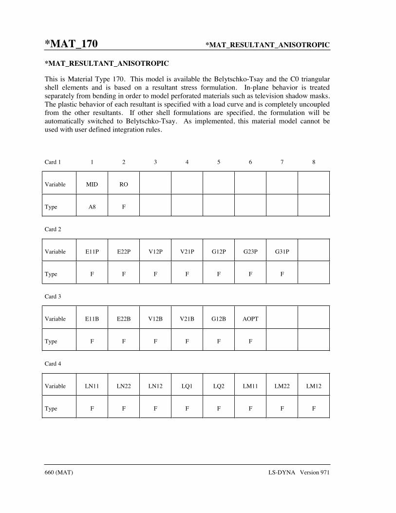
*MAT_170 *MAT_RESULTANT_ANISOTROPIC
660 (MAT) LS-DYNA Version 971
*MAT_RESULTANT_ANISOTROPIC
This is Material Type 170. This model is available the Belytschko-Tsay and the C0 triangular shell elements and is based on a resultant stress formulation. In-plane behavior is treated separately from bending in order to model perforated materials such as television shadow masks. The plastic behavior of each resultant is specified with a load curve and is completely uncoupled from the other resultants. If other shell formulations are specified, the formulation will be automatically switched to Belytschko-Tsay. As implemented, this material model cannot be used with user defined integration rules.
Card 1 1 2 3 4 5 6 7 8
Variable MID RO
Type A8 F
Card 2
Variable E11P E22P V12P V21P G12P G23P G31P
Type F F F F F F F
Card 3
Variable E11B E22B V12B V21B G12B AOPT
Type F F F F F F
Card 4
Variable LN11 LN22 LN12 LQ1 LQ2 LM11 LM22 LM12
Type F F F F F F F F

*MAT_RESULTANT_ANISOTROPIC *MAT_170
LS-DYNA Version 971 661 (MAT)
Card 5 1 2 3 4 5 6 7 8
Variable A1 A2 A3
Type F F F
Card 6
Variable V1 V2 V3 D1 D2 D3 BETA
Type F F F F F F F
VARIABLE DESCRIPTION
MID Material identification. A unique number or label not exceeding 8 characters must be specified.
RO Mass density.
E11P E11p, for in plane behavior.
E22P E22p, for in plane behavior.
V12P ν12p, for in plane behavior.
V11P ν21p, for in plane behavior.
G12P G12p, for in plane behavior.
G23P G23p, for in plane behavior.
G31P G31p, for in plane behavior.
E11B E11b, for bending behavior.
E22B E22b, for bending behavior.
V12B ν12b, for bending behavior.
V21B ν21b, for bending behavior.

*MAT_170 *MAT_RESULTANT_ANISOTROPIC
662 (MAT) LS-DYNA Version 971
VARIABLE DESCRIPTION
G12B G12b, for bending behavior.
AOPT Material axes option (see MAT_OPTION TROPIC_ELASTIC for a more complete description):
EQ.0.0: locally orthotropic with material axes determined by element nodes 1, 2, and 4, as with *DEFINE_COORDINATE_ NODES.
EQ.2.0: globally orthotropic with material axes determined by vectors defined below, as with *DEFINE_COORDINATE_ VECTOR.
EQ.3.0: locally orthotropic material axes determined by rotating the material axes about the element normal by an angle, BETA, from a line in the plane of the element defined by the cross product of the vector v with the element normal.
LT.0.0: the absolute value of AOPT is a coordinate system ID number (CID on *DEFINE_COORDINATE_NODES, *DEFINE_ COORDINATE_SYSTEM or *DEFINE_COORDINATE_ VECTOR). Available in R3 version of 971 and later.
LN11 Yield curve ID for N11.
LN22 Yield curve ID for N22.
LN12 Yield curve ID for N12.
LQ1 Yield curve ID for Q1.
LQ2 Yield curve ID for Q2.
LM11 Yield curve ID for M11.
LM22 Yield curve ID for M22.
LM12 Yield curve ID for M12.
A1,A2,A3 a1 a2 a3, define components of vector a for AOPT = 2.
V1,V2,V3 v1 v2 v3, define components of vector v for AOPT = 3.
D1,D2,D3 d1 d2 d3, define components of vector d for AOPT = 2.
BETA Material angle in degrees for AOPT = 3, may be overridden on the element card, see *ELEMENT_SHELL_BETA.

*MAT_RESULTANT_ANISOTROPIC *MAT_170
LS-DYNA Version 971 663 (MAT)
Remarks:
The in-plane elastic matrix for in-plane, plane stress behavior is given by:
11 12
12 22
44
55
66
0 0 0
0 0 0
0 0 0 0
0 0 0 0
0 0 0 0
p p
p p
in plane p
p
p
Q Q
Q Q
C Q
Q
Q
=
The terms Qijp are defined as:
1111
12 21
2222
12 21
12 1112
12 21
44 12
55 23
66 31
1
1
1
pp
p p
pp
p p
p pp
p p
p p
p p
p p
EQ
EQ
EQ
Q G
Q G
Q G
ν ν
ν νν
ν ν
=−
=−
=−
=
=
=
The elastic matrix for bending behavior is given by:
11 12
12 22
44
0
0
0 0
b b
bending b b
b
Q Q
C Q Q
Q
=
The terms Qijp are similarly defined.

*MAT_171 *MAT_STEEL_CONCENTRIC_BRACE
664 (MAT) LS-DYNA Version 971
*MAT_STEEL_CONCENTRIC_BRACE
This is Material Type 171. It represents the cyclic buckling and tensile yielding behavior of steel braces and is intended primarily for seismic analysis. Use only for beam elements with ELFORM=2 (Belytschko-Schwer beam).
Note: This Material Type will be available starting in release 3 of version 971.
Card 1 1 2 3 4 5 6 7 8
Variable MID RO YM PR SIGY LAMDA FBUCK FBUCK2
Type A8 F F F F F F F
Default none none none none none See
RemarksSee
Remarks 0.0
Card 2
Variable CCBRF BCUR
Type F F
Default See
Remarks
Card 3
Variable TS1 TS2 TS3 TS4 CS1 CS2 CS3 CS4
Type F F F F F F F F
Default 0 0 0 0 =TS1 =TS2 =TS3 =TS4

*MAT_STEEL_CONCENTRIC_BRACE *MAT_171
LS-DYNA Version 971 665 (MAT)
VARIABLE DESCRIPTION
MID Material identification. A unique number or label not exceeding 8 characters must be specified.
RO Mass density
YM Young’s Modulus
PR Poisson’s Ratio
SIGY Yield stress
LAMDA Slenderness ratio (optional – see note)
FBUCK Initial buckling load (optional – see note. If used, should be positive)
FBUCK2 Optional extra term in initial buckling load – see note
CCBRF Reduction factor on initial buckling load for cyclic behavior
BCUR Optional load curve giving compressive buckling load (y-axis) versus compressive strain (x-axis - both positive)
TS1-TS4 Tensile axial strain thresholds 1 to 4
CS1-CS4 Compressive axial strain thresholds 1 to 4
Remarks:
The brace element is intended to represent the buckling, yielding and cyclic behavior of steel elements such as tubes or I-sections that carry only axial loads. Empirical relationships are used to determine the buckling and cyclic load-deflection behavior. A single beam element should be used to represent each structural element.
The cyclic behavior is shown in the graph (compression shown as negative force and displacement).

*MAT_171 *MAT_STEEL_CONCENTRIC_BRACE
666 (MAT) LS-DYNA Version 971
Figure 171.1
The initial buckling load (point 2) is:
22 /b initialF FBUCK FBUCK L= +
where FBUCK, FBUCK2 are input parameters and L is the length of the beam element. If neither FBUCK nor FBUCK2 are defined, the default is that the initial buckling load is
( )SIGY A A cross sectional area∗ = − .
The buckling curve (shown dashed) has the form:
( ) /b initialF d F A Bδ= +
where δ is abs(strain/yield strain), and A and B are internally-calculated functions of slenderness ratio (λ) and loading history.
The member slenderness ratio λ is defined as kL
r, where k depends on end conditions, L is the
element length, and r is the radius of gyration such that 2Ar I= (and ( )min ,yy zzI I I= ); λ will
by default be calculated from the section properties and element length using k=1. Optionally, this may be overridden by input parameter LAMDA to allow for different end conditions.
Optionally, the user may provide a buckling curve (BCUR). The points of the curve give compressive displacement (x-axis) versus force (y-axis); the first point should have zero displacement and the initial buckling force. Displacement and force should both be positive. The initial buckling force must not be greater than the yield force.
1
23
4
5
6
7
9
8
16 17
10
11,13
12
14
15
18
19

*MAT_STEEL_CONCENTRIC_BRACE *MAT_171
LS-DYNA Version 971 667 (MAT)
The tensile yield force (point 5 and section 16-17) is defined by
yF SIGY A= ∗ ,
where yield stress SIGY is an input parameter and A is the cross-sectional area.
Following initial buckling and subsequent yield in tension, the member is assumed to be damaged. The initial buckling curve is then scaled by input parameter CCBRF, leading to reduced strength curves such as segments 6-7, 10-14 and 18-19. This reduction factor is typically in the range 0.6 to 1.0 (smaller values for more slender members). By default, CCBRF is calculated using SEAOC 1990:
1
0.51
c
CCBRF
Cλ
=+
and0.5c
y
EC π
σ=
When tensile loading is applied after buckling, the member must first be straightened before the full tensile yield force can be developed. This is represented by a reduced unloading stiffness (e.g. segment 14-15) and the tensile reloading curve (segments 8-9 and 15-16). Further details can be found in Bruneau, Uang, and Whittaker [1998] and Structural Engineers Association of California [1974, 1990, 1996].
Figure 171.2
The response of stocky (low λ) and slender (high λ) braces are compared in the graph. These differences are achieved by altering the input value LAMDA (or the section properties of the beam) and FBUCK.
Output Axial Strain and Internal Energy may be plotted from the INTEGRATED beam results menus in Oasys D3PLOT and T/HIS.
Solid line: λ=25 (stocky) Dashed line: λ=120 (slender)
*MAT_171 *MAT_STEEL_CONCENTRIC_BRACE
668 (MAT) LS-DYNA Version 971
FEMA thresholds are the total axial strains (defined by change of length/initial length) at which the element is deemed to have passed from one category to the next, e.g. “Elastic”, “Immediate Occupancy”, “Life Safe”, etc. During the analysis, the maximum tensile and compressive strains (“high tide strains”) are recorded. These are checked against the user-defined limits TS1 to TS4 and CS1 to CS4. The output flag is then set to 0, 1, 2, 3, or 4 according to which limits have been passed. The value in the output files is the highest such flag from tensile or compressive strains. To plot this data, select INTEGRATED beam results, Integration point 4, Axial Strain.
Maximum plastic strains in tension and compression are also output. These are defined as maximum total strain to date minus the yield or first buckling strain for tensile and compressive plastic strains respectively. To plot these, select INTEGRATED beam results, Integration point 4, “shear stress XY” and “shear stress XZ” for tensile and compressive plastic strains, respectively.

*MAT_CONCRETE_EC2 *MAT_172
LS-DYNA Version 971 669 (MAT)
*MAT_CONCRETE_EC2
This is Material Type 172, for shell and Hughes-Liu beam elements only. The material model can represent plain concrete only, reinforcing steel only, or a smeared combination of concrete and reinforcement. The model includes concrete cracking in tension and crushing in compression, and reinforcement yield, hardening and failure. Properties are thermally sensitive; the material model can be used for fire analysis. Material data and equations governing the behavior (including thermal properties) are taken from Eurocode 2 Part 1.2 (General rules – Structural fire design).
Note: This Material Type will be available starting in release 3 of version 971.
Card 1 1 2 3 4 5 6 7 8
Variable MID RO FC FT TYPEC UNITC
Type A8 F F F F F
Default none none none 0.0 1.0 1.0
Card 2
Variable ESOFT LCHAR MU
Type A8 F F
Default See notes 0.0 0.4
Card 3
Variable YMREINF PRREINF SUREINF TYPER FRACRX FRACY
Type F F F F F F
Default none 0.0 0.0 1.0 0.0 0.0

*MAT_172 *MAT_CONCRETE_EC2
670 (MAT) LS-DYNA Version 971
Card 4 - Leave blank
Card 4 1 2 3 4 5 6 7 8
Variable
Type
Default
VARIABLE DESCRIPTION
MID Material identification. A unique number or label not exceeding 8 characters must be specified.
RO Mass density
FC Compressive strength of concrete (stress units)
FT Tensile stress to cause cracking
TYPEC Concrete aggregate type for stress-strain-temperature relationships EQ.1.0: Siliceous (default)
EQ.2.0: Calcareous
UNITC Factor to convert stress units to MPa (see Remarks)
ESOFT Tension stiffening (Slope of stress-strain curve post-cracking in tension)
MU Friction on crack planes (max shear = mu*compressive stress)
LCHAR Characteristic length at which ESOFT applies
YMREINF Young’s Modulus of reinforcement
PRREINF Poisson’s Ratio of reinforcement
SUREINF Ultimate stress of reinforcement
TYPER Type of reinforcement for stress-strain-temperature relationships EQ.1.0: Hot rolled reinforcing steel EQ.2.0: Cold worked reinforcing steel (default) EQ.3.0: Quenched and tempered prestressing steel EQ.4.0: Cold worked prestressing steel

*MAT_CONCRETE_EC2 *MAT_172
LS-DYNA Version 971 671 (MAT)
VARIABLE DESCRIPTION
FRACRX Fraction of reinforcement (x-axis) (e.g. for 1% reinforcement FRACR=0.01)
FRACRY Fraction of reinforcement (y-axis) (e.g. for 1% reinforcement FRACR=0.01)
Remarks:
Reinforcement is treated as separate sets of bars in the local element x and y axes. The reinforcement is assumed not to carry through-thickness or in-plane shear.
Creating Reinforced Concrete Sections This material model can be used to represent unreinforced concrete (FRACR=0), steel (FRACR=1), or reinforced concrete with evenly distributed reinforcement (0<FRACR<1).
Alternatively, use *INTEGRATION_SHELL to define the section. All parts referred to by one integration rule must have the same material type, but can have different material properties.Create one Part for concrete, and another for steel.
Material Behavior Stress-strain curves for concrete and steel are as specified in EC2, scaled to the user-supplied FC, FT and SUREINF. Thermal expansion data is taken from EC2 directly, there is no option at present to override with user-supplied data.
Cracking in tension occurs when the maximum in-plane principal stress (bending + membrane stress at an integration point) reaches FT. Thereafter, increasing tensile strain leads to stress reduction according to the stress/strain slope ESOFT (default = 5 times initial elastic stiffness). Infinite ESOFT would in theory correspond to instantaneous loss of tensile capacity due to cracking, but values higher than the initial elastic modulus are not allowed. Finite values imply an amount of energy absorption needed to create a fully open crack, which arises in practice from the reinforcement holding the concrete together allowing it to continue to take some tension (this effect is frequently known as tension-stiffening). LCHAR can be used to maintain constant energy per unit area of crack irrespective of mesh size if desired – the value of ESOFT is scaled up for larger elements and down for smaller ones such that the stress-versus-displacement relation is the same. However, tension-stiffening effects are usually characterized by strain rather than displacement, this is obtained by LCHAR=0. If no data is available, it is recommended to set ESOFT such that FT/ESOFT = 0.0025, i.e. at a tensile strain of 0.0025 the crack is fully open, and LCHAR=0.
Output“Plastic Strain” is the maximum of the plastic strains in the reinforcement in the two local directions.
Extra history variables may be requested for shell elements (NEIPS on *DATABASE_ EXTENT_BINARY), which have the following meaning:

*MAT_172 *MAT_CONCRETE_EC2
672 (MAT) LS-DYNA Version 971
Extra Variable 1: Current crack opening strain (if two cracks are present, max of the two) Extra Variable 2: Equivalent uniaxial strain for concrete compressive behavior Extra Variable 3: Number of cracks (0, 1 or 2) Extra Variable 4: Temperature Extra Variable 5: Thermal strain Extra Variable 6: Current crack opening strain – first crack to form Extra Variable 7: Current crack opening strain – crack at 90 degrees to first crack Extra Variable 8: Max crack opening strain – first crack to form Extra Variable 9: Max crack opening strain – crack at 90 degrees to first crack
MAXINT (shells) and/or BEAMIP (beams) on *DATABASE_EXTENT_BINARY should be set to the maximum number of integration points, so that results for all integration points can be plotted separately.
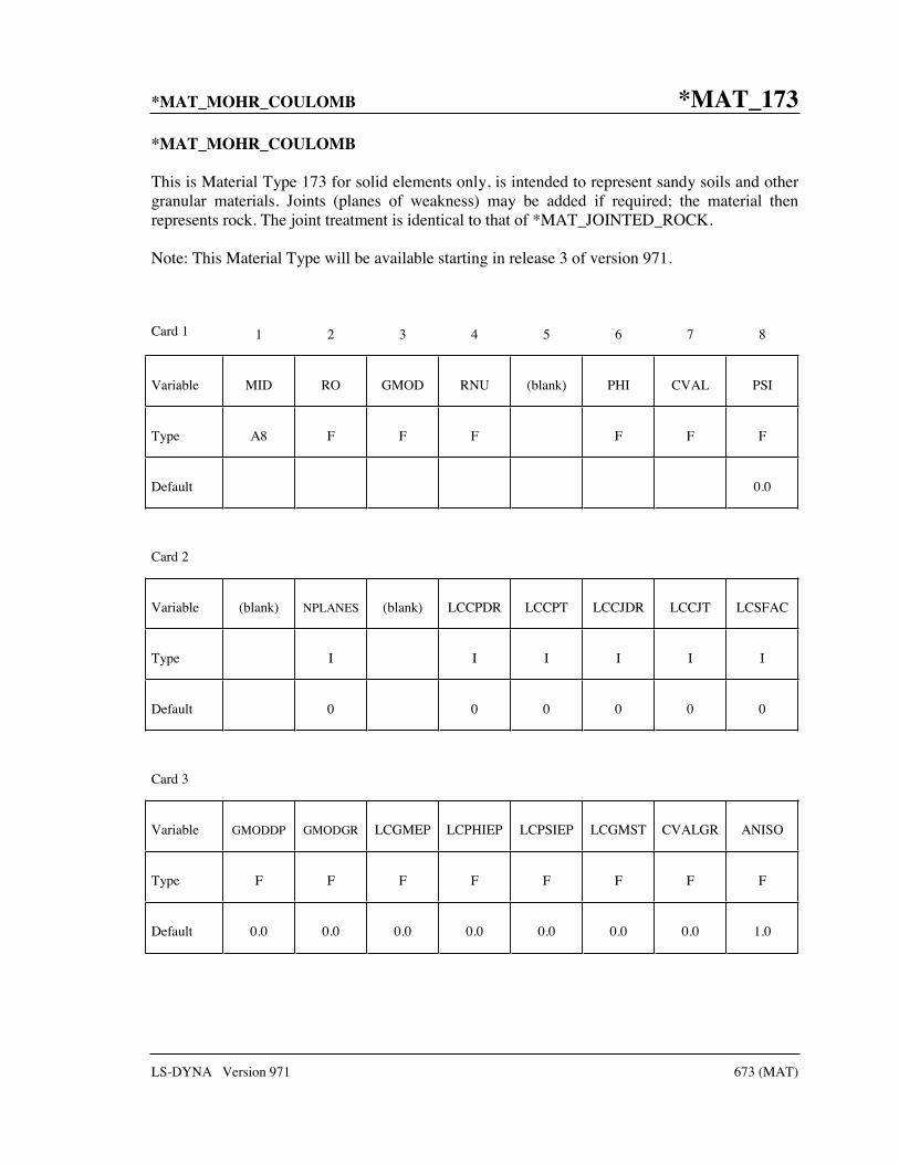
*MAT_MOHR_COULOMB *MAT_173
LS-DYNA Version 971 673 (MAT)
*MAT_MOHR_COULOMB
This is Material Type 173 for solid elements only, is intended to represent sandy soils and other granular materials. Joints (planes of weakness) may be added if required; the material then represents rock. The joint treatment is identical to that of *MAT_JOINTED_ROCK.
Note: This Material Type will be available starting in release 3 of version 971.
Card 1 1 2 3 4 5 6 7 8
Variable MID RO GMOD RNU (blank) PHI CVAL PSI
Type A8 F F F F F F
Default 0.0
Card 2
Variable (blank) NPLANES (blank) LCCPDR LCCPT LCCJDR LCCJT LCSFAC
Type I I I I I I
Default 0 0 0 0 0 0
Card 3
Variable GMODDP GMODGR LCGMEP LCPHIEP LCPSIEP LCGMST CVALGR ANISO
Type F F F F F F F F
Default 0.0 0.0 0.0 0.0 0.0 0.0 0.0 1.0

*MAT_173 *MAT_MOHR_COULOMB
674 (MAT) LS-DYNA Version 971
Card 4 – Repeat for each plane (maximum 3 planes)
Card 4 1 2 3 4 5 6 7 8
Variable DIP DIPANG CPLANE FRPLANE TPLANE SHRMAX LOCAL
Type F F F F F F F
Default 0.0 0.0 0.0 0.0 0.0 1.e20 0.0
VARIABLE DESCRIPTION
MID Material identification. A unique number or label not exceeding 8 characters must be specified.
RO Mass density
GMOD Elastic shear modulus
RNU Poisson’s ratio
PHI Angle of friction (radians)
CVAL Cohesion value (shear strength at zero normal stress)
PSI Dilation angle (radians)
NPLANES Number of joint planes (maximum 3)
LCCPDR Load curve for extra cohesion for parent material (dynamic relaxation)
LCCPT Load curve for extra cohesion for parent material (transient)
LCCJDR Load curve for extra cohesion for joints (dynamic relaxation)
LCCJT Load curve for extra cohesion for joints (transient)
LCSFAC Load curve giving factor on strength vs. time
GMODDP Z-coordinate at which GMOD and CVAL are correct
GMODGR Gradient of GMOD versus z-coordinate (usually negative)
LCGMEP Load curve of GMOD versus plastic strain (overrides GMODGR)
LCPHIEP Load curve of PHI versus plastic strain

*MAT_MOHR_COULOMB *MAT_173
LS-DYNA Version 971 675 (MAT)
VARIABLE DESCRIPTION
LCPSIEP Load curve of PSI versus plastic strain
LCGMST (Leave blank)
CVALGR Gradient of CVAL versus z-coordinate (usually negative)
ANISO Factor applied to elastic shear stiffness in global XZ and YZ planes
DIP Angle of the plane in degrees below the horizontal
DIPANG Plan view angle (degrees) of downhill vector drawn on the plane
CPLANE Cohesion for shear behavior on plane
PHPLANE Friction angle for shear behavior on plane (degrees)
TPLANE Tensile strength across plane (generally zero or very small)
SHRMAX Max shear stress on plane (upper limit, independent of compression)
LOCAL EQ.0: DIP and DIPANG are with respect to the global axes EQ.1: DIP and DIPANG are with respect to the local element axes
Remarks:
1. The material has a Mohr Coulomb yield surface, given by τmax = C + σntan(phi), where τmax =maximum shear stress on any plane, σn=normal stress on that plane (positive in compression), C=cohesion, phi=friction angle. The plastic potential function is of the form βσk - σI + constant, where σk = maximum principal stress, σi = minimum principal
stress, and ( )( )( )
1 sin
1 sin
psi
psiβ
+=
−.
2. The tensile strength of the material is given by ( )max tan
C
phiσ = where C is the cohesion.
After the material reaches its tensile strength, further tensile straining leads to volumetric voiding; the voiding is reversible if the strain is reversed.
3. If depth-dependent properties are used, the model must be oriented with the z-axis in the upward direction.
4. Plastic strain is defined as SQRT(2/3.εpij.εpij), i.e. the same way as for other elasto-plastic material models.
5. Friction and dilation angles PHI and PSI may vary with plastic strain, to model heavily consolidated materials under large shear strains – as the strain increases, the dilation angle typically reduces to zero and the friction angle to a lower, pre-consolidation value.

*MAT_173 *MAT_MOHR_COULOMB
676 (MAT) LS-DYNA Version 971
6. For similar reasons, the shear modulus may reduce with plastic strain, but this option may sometimes give unstable results.
7. The loadcurves LCCPDR, LCCPT, LCCJDR, LCCJT allow extra cohesion to be specified as a function of time. The cohesion is additional to that specified in the material parameters. This is intended for use during the initial stages of an analysis to allow application of gravity or other loads without cracking or yielding, and for the cracking or yielding then to be introduced in a controlled manner. This is done by specifying extra cohesion that exceeds the expected stresses initially, then declining to zero. If no curves are specified, no extra cohesion is applied.
8. The loadcurve for factor on strength applies simultaneously to the cohesion and tan(friction angle) of parent material and all joints. This feature is intended for reducing the strength of the material gradually, to explore factors of safety. If no curve is present, a constant factor of 1 is assumed. Values much greater than 1.0 may cause problems with stability.
9. The anisotropic factor ANISO applies the elastic shear stiffness in the global XZ and YZ planes. It can be used only in pure Mohr-Coulomb mode (NPLANES=0).
10. To model soil, set NJOINT=0. The joints are to allow modeling of rock, and are treated identically to those of *MAT_JOINTED_ROCK.
11. The joint plane orientations are defined by the angle of a “downhill vector” drawn on the plane, i.e. the vector is oriented within the plane to obtain the maximum possible downhill angle. DIP is the angle of this line below the horizontal. DIPANG is the plan-view angle of the line (pointing down hill) measured clockwise from the global Y-axis about the global Z-axis.
12. Joint planes would generally be defined in the global axis system if they are taken from survey data. However, the material model can also be used to represent masonry, in which case the weak planes represent the cement and lie parallel to the local element axes.
13. The joint planes rotate with the rigid body motion of the elements, irrespective of whether their initial definitions are in the global or local axis system.
14. Extra variables for plotting. By setting NEIPH on *DATABASE_EXTENT_BINARY to 15, the following variables can be plotted in D3PLOT and T/HIS:
Extra Variable 1: Mobilized strength fraction for base material Extra Variable 2: Volumetric void strain Extra Variable 3: Maximum stress overshoot during plastic calculation Extra Variable 4: crack opening strain for plane 1 Extra Variable 5: crack opening strain for plane 2 Extra Variable 6: crack opening strain for plane 3 Extra Variable 7: crack accumulated shear strain for plane 1 Extra Variable 8: crack accumulated shear strain for plane 2 Extra Variable 9: crack accumulated shear strain for plane 3

*MAT_MOHR_COULOMB *MAT_173
LS-DYNA Version 971 677 (MAT)
Extra Variable 10: current shear utilization for plane 1 Extra Variable 11: current shear utilization for plane 2 Extra Variable 12: current shear utilization for plane 3 Extra Variable 13: maximum shear utilization to date for plane 1 Extra Variable 14: maximum shear utilization to date for plane 2 Extra Variable 15: maximum shear utilization to date for plane 3

*MAT_174 *MAT_RC_BEAM
678 (MAT) LS-DYNA Version 971
*MAT_RC_BEAM
This is Material Type 174, for Hughes-Liu beam elements only. The material model can represent plain concrete only, reinforcing steel only, or a smeared combination of concrete and reinforcement. The main emphasis of this material model is the cyclic behavior – it is intended primarily for seismic analysis.
Note: This Material Type will be available starting in release 3 of version 971.
Card 1 1 2 3 4 5 6 7 8
Variable MID RO EUNL PR FC EC1 EC50 RESID
Type A8 F F F F F F F
Default none none See
Remarks 0.0 none 0.0022 See
Remarks 0.2
Card 2
Variable FT UNITC (blank) (blank) (blank) ESOFT LCHAR OUTPUT
Type F F F F F F F F
Default See
Remarks 1.0 none none none See
Remarks none 0
Card 3
Variable FRACR YMREINF PRREINF SYREINF SUREINF ESHR EUR RREINF
Type F F F F F F F F
Default 0.0 none 0.0 0.0 SYREINF 0.03 0.2 4.0

*MAT_RC_BEAM *MAT_174
LS-DYNA Version 971 679 (MAT)
VARIABLE DESCRIPTION
MID Material identification. A unique number or label not exceeding 8 characters must be specified.
RO Mass density
EUNL Initial unloading elastic modulus (See Remarks).
PR Poisson’s ratio.
FC Cylinder strength (stress units)
EC1 Strain at which stress FC is reached.
EC50 Strain at which the stress has dropped to 50% FC
RESID Residual strength factor
FT Maximum tensile stress
UNITC Factor to convert stress units to MPa (See Remarks)
ESOFT Slope of stress-strain curve post-cracking in tension
LCHAR Characteristic length for strain-softening behavior
OUTPUT Output flag controlling what is written as “plastic strain” EQ.0.0: Curvature EQ.1.0: “High-tide” plastic strain in reinforcement
FRACR Fraction of reinforcement (e.g. for 1% reinforcement FRACR=0.01)
YMREINF Young’s Modulus of reinforcement
PRREINF Poisson’s Ratio of reinforcement
SYREINF Yield stress of reinforcement
SUREINF Ultimate stress of reinforcement
ESHR Strain at which reinforcement begins to harden
EUR Strain at which reinforcement reaches ultimate stress
R_REINF Dimensionless Ramberg-Osgood parameter r. If zero, a default value r=4.0 will be used. If set to -1, parameters will be calculated from Kent & Park formulae. (See Remarks)

*MAT_174 *MAT_RC_BEAM
680 (MAT) LS-DYNA Version 971
Remarks:
Creating sections for reinforced concrete beams This material model can be used to represent unreinforced concrete (FRACR=0), steel (FRACR=1), or reinforced concrete with evenly distributed reinforcement (0<FRACR<1).
Alternatively, use *INTEGRATION_BEAM to define the section. A new option in allows the user to define a Part ID for each integration point, similar to the facility already available with *INTEGRATION_SHELL. All parts referred to by one integration rule must have the same material type, but can have different material properties. Create one Part for concrete, and another for steel. These Parts should reference Materials, both of type *MAT_RC_BEAM, one with FRACR=0, the other with FRACR=1. Then, by assigning one or other of these Part Ids to each integration point the reinforcement can be applied to the correct locations within the section of the beam.
ConcreteIn monotonic compression, the approach of Park and Kent, as described in Park & Paulay [1975] is used. The material follows a parabolic stress-strain curve up to a maximum stress equal to the cylinder strength FC; therafter the strength decays linearly with strain until the residual strength is reached. Default values for some material parameters will be calculated automatically as follows:
( )3 0.2950
145 1000
FCEC
FC
+=
− (FC in MPa units – Park and Kent, from test data)
EUNL = initial tangent slope = 2FC/EC1 (User-defined values lower than this are not permitted, but higher values may be defined if desired)
2
31.4
10
FCFT = (FC in MPa units – from CEB Code 1993)
ESOFT = EUNL (User-defined values higher than EUNL are not permitted)
UNITC is used only to calculate default values for the above parameters from FC.
Strain-softening behavior tends to lead to deformations being concentrated in one element, and hence the overall force-deflection behavior of the structure can be mesh-size-dependent if the softening is characterized by strain. To avoid this, a characteristic length (LCHAR) may be defined. This is the length of specimen (or element) that would exhibit the defined monotonic stress-strain relationship. LS-DYNA adjusts the stress-strain relationship after ultimate load for each element, such that all elements irrespective of their length will show the same deflection during strain softening (i.e. between ultimate load and residual load). Therefore, although deformation will still be concentrated in one element, the load-deflection behavior should be the same irrespective of element size. For tensile behavior, ESOFT is similarly scaled.

*MAT_RC_BEAM *MAT_174
LS-DYNA Version 971 681 (MAT)
Figure 174.1
Cyclic behavior is broadly suggested by Blakeley and Park [1973] as described in Park & Paulay [1975]; the stress-strain response lies within the Park-Kent envelope, and is characterized by stiff initial unloading response at slope EUNL followed by a less stiff response if it unloads to less than half the current strength. Reloading stiffness degrades with increasing strain.
In tension, the stress rises linearly with strain until a tensile limit FT is reached. Thereafter the stiffness and strength decays with increasing strain at a rate ESOFT. The stiffness also decays such that unloading always returns to strain at which the stress most recently changed to tensile.
Figure 174.2
σy
σult
εultεsh
1
2
3,14
4
5,12
7
7,9
13
10 11
16
MAT RC BEAM - concrete
6
8
15,1920
17
18

*MAT_174 *MAT_RC_BEAM
682 (MAT) LS-DYNA Version 971
Monotonic loading of the reinforcement results in the stress-strain curve shown, which is parabolic between εsh and εult. The same curve acts as an envelope on the hysteretic behavior, when the x-axis is cumulative plastic strain.
Unloading from the yielded condition is elastic until the load reverses. Thereafter, the Bauschinger Effect (reduction in stiffness at stresses less than yield during cyclic deformation) is represented by following a Ramberg-Osgood relationship until the yield stress is reached:
1
1r
sCHE
σ σε εσ
−
− = +
where ε and σ are strain and stress, sε is the strain at zero stress, E is Young’s Modulus, and r
and CHσ are as defined below
Figure 174.3
Two options are given for calculation r and CHσ , which is performed at each stress reversal:
1. If RREINF is input as -1, r and σCH are calculated internally from formulae given in Kent and Park. Parameter r depends on the number of stress reversals. Parameter CHσ depends
on the plastic strain that occurred between the previous two stress reversals. The formulae were statistically derived from experiments, but may not fit all circumstances. In particular, large differences in behavior may be caused by the presence or absence of small stress reversals such as could be caused by high frequency oscillations. Therefore, results might sometimes be unduly sensitive to small changes in the input data.
1
2 3 5
4
6 8
7
9 11
10
12 14 15
13
MAT RC BEAM – reinforcement – RREINF=4.0

*MAT_RC_BEAM *MAT_174
LS-DYNA Version 971 683 (MAT)
2. If RREINF is entered by the user or left blank, r is held constant while CHσ is calculated
on each reversal such that the Ramberg-Osgood curve meets the monotonic stress-strain curve at the point from which it last unloaded, e.g. points 6 and 8 are coincident in the graph below. The default setting RREINF=4.0 gives similar hysteresis behavior to that described by Kent & Park but is unlikely to be so sensitive to small changes of input data.
OutputIt is recommended to use BEAMIP on *DATABASE_EXTENT_BINARY to request stress and strain output at the individual integration points. If this is done, for MAT_RC_BEAM only, element curvature is written to the output files in place of plastic strain. In the post-processor, select “plastic strain” to display curvature (whichever of the curvatures about local y and z axes has greatest absolute value will be plotted). Alternatively, select “axial strain” to display the total axial strain (elastic + plastic) at that integration point; this can be combined with axial stress to create hysteresis plots such as those shown above.

*MAT_175 *MAT_VISCOELASTIC_THERMAL
684 (MAT) LS-DYNA Version 971
*MAT_VISCOELASTIC_THERMAL
This is Material Type 175. This material model provides a general viscoelastic Maxwell model having up to 12 terms in the prony series expansion and is useful for modeling dense continuum rubbers and solid explosives. Either the coefficients of the prony series expansion or a relaxation curve may be specified to define the viscoelastic deviatoric and bulk behavior.
Card 1 1 2 3 4 5 6 7 8
Variable MID RO BULK PCF EF TREF A B
Type A8 F F F F F F F
Insert a blank card here if constants are defined on cards 3,4,... below.
If an elastic layer is defined in a laminated shell this card must be blank.
Card 2 1 2 3 4 5 6 7 8
Variable LCID NT BSTART TRAMP LCIDK NTK BSTARTK TRAMPK
Type F I F F F I F F
Card Format for viscoelastic constants. Up to 12 cards may be input. A keyword card (with a “*” in column 1) terminates this input if less than 12 cards are used. These cards are not needed if relaxation data is defined. The number of terms for the shear behavior may differ from that for the bulk behavior: simply insert zero if a term is not included.
If an elastic layer is defined you only need to define GI and KI (note in an elastic layer only one card is needed)
Optional Cards
1 2 3 4 5 6 7 8
Variable GI BETAI KI BETAKI
Type F F F F

*MAT_VISCOELASTIC_THERMAL *MAT_175
LS-DYNA Version 971 685 (MAT)
VARIABLE DESCRIPTION
MID Material identification. A unique number or label not exceeding 8 characters must be specified.
RO Mass density.
BULK Elastic bulk modulus.
PCF Tensile pressure elimination flag for solid elements only. If set to unity tensile pressures are set to zero.
EF Elastic flag (if equal 1, the layer is elastic. If 0 the layer is viscoelastic).
TREF Reference temperature for shift function (must be greater than zero).
A Coefficient for the Arrhenius and the Williams-Landau-Ferry shift functions.
B Coefficient for the Williams-Landau-Ferry shift function.
LCID Load curve ID for deviatoric behavior if constants, Gi, and βi are determined via a least squares fit. This relaxation curve is shown below.
NT Number of terms in shear fit. If zero the default is 6. Fewer than NT terms will be used if the fit produces one or more negative shear moduli. Currently, the maximum number is set to 6.
BSTART In the fit, β1 is set to zero, β2 is set to BSTART, β3 is 10 times β2, β4
is 100 times greater than β3 , and so on. If zero, BSTART is determined by an iterative trial and error scheme.
TRAMP Optional ramp time for loading.
LCIDK Load curve ID for bulk behavior if constants, Ki, and βκi are determined via a least squares fit. This relaxation curve is shown below.
NTK Number of terms desired in bulk fit. If zero the default is 6. Currently, the maximum number is set to 6.
BSTARTK In the fit, βκ1 is set to zero, βκ2 is set to BSTARTK, βκ3 is 10 times βκ2, βκ4 is 100 times greater than βκ3 , and so on. If zero, BSTARTK is determined by an iterative trial and error scheme.
TRAMPK Optional ramp time for bulk loading.
GI Optional shear relaxation modulus for the ith term
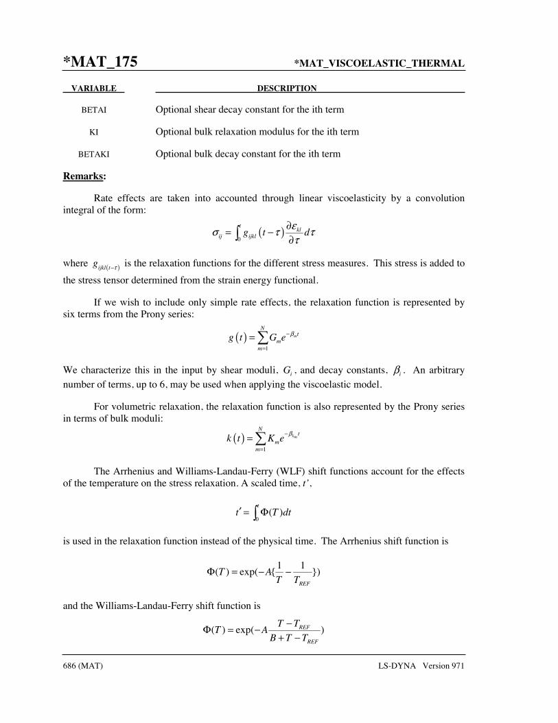
*MAT_175 *MAT_VISCOELASTIC_THERMAL
686 (MAT) LS-DYNA Version 971
VARIABLE DESCRIPTION
BETAI Optional shear decay constant for the ith term
KI Optional bulk relaxation modulus for the ith term
BETAKI Optional bulk decay constant for the ith term
Remarks:
Rate effects are taken into accounted through linear viscoelasticity by a convolution integral of the form:
( )0
tkl
ij ijklg t dεσ τ ττ
∂= −∂
where ( )ijkl tg τ− is the relaxation functions for the different stress measures. This stress is added to
the stress tensor determined from the strain energy functional.
If we wish to include only simple rate effects, the relaxation function is represented by six terms from the Prony series:
( )1
m
Nt
mm
g t G e β−
==
We characterize this in the input by shear moduli, iG , and decay constants, iβ . An arbitrary
number of terms, up to 6, may be used when applying the viscoelastic model.
For volumetric relaxation, the relaxation function is also represented by the Prony series in terms of bulk moduli:
( )1
km
Nt
mm
k t K eβ−
==
The Arrhenius and Williams-Landau-Ferry (WLF) shift functions account for the effects of the temperature on the stress relaxation. A scaled time, t’,
0( )
tt T dt′ = Φ
is used in the relaxation function instead of the physical time. The Arrhenius shift function is
1 1( ) exp( { })
REF
T AT T
Φ = − −
and the Williams-Landau-Ferry shift function is
( ) exp( )REF
REF
T TT A
B T T
−Φ = −+ −

*MAT_VISCOELASTIC_THERMAL *MAT_175
LS-DYNA Version 971 687 (MAT)
If all three values (TREF, A, and B) are not zero, the WLF function is used; the Arrhenius function is used if B is zero; and no scaling is applied if all three values are zero.
Figure 175.1. Relaxation curve. This curve defines stress versus time where time is defined on a logarithmic scale. For best results, the points defined in the load curve should be equally spaced on the logarithmic scale. Furthermore, the load curve should be smooth and defined in the positive quadrant. If nonphysical values are determined by least squares fit, LS-DYNA will terminate with an error message after the initialization phase is completed. If the ramp time for loading is included, then the relaxation which occurs during the loading phase is taken into account. This effect may or may not be important.

*MAT_176 *MAT_QUASILINEAR_VISCOELASTIC
688 (MAT) LS-DYNA Version 971
*MAT_QUASILINEAR_VISCOELASTIC
Purpose: This is Material Type 176. This is a quasi-linear, isotropic, viscoelastic material based on a one-dimensional model by Fung [1993], which represents biological soft tissues such as brain, skin, kidney, spleen, etc. This model is implemented for solid and shell elements. The formulation has recently been changed to allow larger strains, and, in general, will not give the same results as the previous implementation which remains the default.
Card 1 1 2 3 4 5 6 7 8
Variable MID RO K LC1 LC2 N GSTART M
Type A8 F F I I F F F
Default none none none 0 0 6 1/TMAX 6
Card 2
Variable SO E_MIN E_MAX GAMA1 GAMA2 K EH FORM
Type F F F F F F F I
Default 0.0 -0.9 5.1 0.0 0.0 0.0 0.0 0
Define the following 3 cards if and only if LC1 is 0.
Card 3 1 2 3 4 5 6 7 8
Variable G1 BETA1 G2 BETA2 G3 BETA3 G4 BETA4
Type F F F F F F F F

*MAT_QUASILINEAR_VISCOELASTIC *MAT_176
LS-DYNA Version 971 689 (MAT)
Card 4 1 2 3 4 5 6 7 8
Variable G5 BETA5 G6 BETA6 G7 BETA7 G8 BETA8
Type F F F F F F F F
Card 5
Variable G9 BETA9 G10 BETA10 G11 BETA11 G12 BETA12
Type F F F F F F F F
Define the following card if and only if LC2 is 0.
Card 3 or 6 1 2 3 4 5 6 7 8
Variable C1 C2 C3 C4 C5 C6
Type F F F F F F
VARIABLE DESCRIPTION
MID Material identification. A unique number or label not exceeding 8 characters must be specified.
RO Mass density.
K Bulk modulus.
LC1 Load curve ID that defines the relaxation function in shear. This curve is used to fit the coefficients Gi and BETAi. If zero, define the coefficients directly. The latter is recommended.
LC2 Load curve ID that defines the instantaneous elastic response in compression and tension. If zero, define the coefficients directly. Symmetry is not assumed if only the tension side is define; therefore, defining the response in tension only, may lead to nonphysical behavior in compression. Also, this curve should give a softening response for increasing strain without any negative or zero slopes. A stiffening curve or one with negative slopes is generally unstable.

*MAT_176 *MAT_QUASILINEAR_VISCOELASTIC
690 (MAT) LS-DYNA Version 971
VARIABLE DESCRIPTION
N Number of terms used in the Prony series, a number less than or equal to 6. This number should be equal to the number of decades of time covered by the experimental data. Define this number if LC1 is nonzero. Carefully check the fit in the D3HSP file to ensure that it is valid, since the least square fit is not always reliable.
GSTART Starting value for least square fit. If zero, a default value is set equal to the inverse of the largest time in the experiment. Define this number if LC1 is nonzero.
M Number of terms used to determine the instantaneous elastic response. This variable is ignored with the new formulation but is kept for compatibility with the previous input.
SO Strain (logarithmic) output option to control what is written as component 7 to the d3plot database. (LS-Prepost always blindly labels this component as effective plastic strain.) The maximum values are updated for each element each time step:
EQ.0.0: maximum principal strain that occurs during the calculation,
EQ.1.0: maximum magnitude of the principal strain values that occurs during the calculation,
EQ.2.0: maximum effective strain that occurs during the calculation.
E_MIN Minimum strain used to generate the load curve from Ci. The default range is -0.9 to 5.1. The computed solution will be more accurate if the user specifies the range used to fit the Ci. Linear extrapolation is used outside the specified range.
E_MAX Maximum strain used to generate the load curve from Ci.
K Material failure parameter that controls the volume enclosed by the failure surface, see *MAT_SIMPLIFIED_RUBBER.
LE.0.0: ignore failure criterion; GT.0.0: use actual K value for failure criterions.
GAMA1 Material failure parameter, see *MAT_SIMPLIFIED_RUBBER and Figure 181.1.
GAMA2 Material failure parameter, see *MAT_SIMPLIFIED_RUBBER.
EH Damage parameter, see *MAT_SIMPLIFIED_RUBBER.

*MAT_QUASILINEAR_VISCOELASTIC *MAT_176
LS-DYNA Version 971 691 (MAT)
VARIABLE DESCRIPTION
FORM Formulation of model. FORM=0 gives the original model developed by Fung, which always relaxes to a zero stress state as time approaches infinity, and FORM=1 gives the alternative model, which relaxes to the quasi-static elastic response. In general, the two formulations won’t give the same responses. Formulation, FORM=-1, is an improvement on FORM=0 where the instantaneous elastic response is used in the viscoelastic stress update, not just in the relaxation, as in FORM=0. Consequently, the constants for the elastic response do not need to be scaled.
Gi Coefficients of the relaxation function. The number of coefficients is currently limited to 6 although 12 may be read in to maintain compatibility with the previous formulation’s input. Define these coefficients if LC1 is set to zero. At least 2 coefficients must be nonzero.
BETAi Decay constants of the relaxation function. Define these coefficients if LC1 is set to zero. The number of coefficients is currently limited to 6 although 12 may be read in to maintain compatibility with the previous formulation’s input.
Ci Coefficients of the instantaneous elastic response in compression and tension. Define these coefficients only if LC2 is set to zero.
Remarks:
The equations for the original model (FORM=0) are given as:
( ) ( ) ( )
( )
( )
0
1
1
t
V
nt
ii
ki
ii
t G t d
G t G e
C
ε
β
ε
∂σ ε τ ∂εσ τ τ∂ε ∂τ
σ ε ε
−
=
=
= −
=
=
where G is the shear modulus. Effective plastic strain (which can be written to the d3plot database) is calculated as follows:
2
3effectuve
ij ijε ε ε=
The polynomial for instantaneous elastic response should contain only odd terms if symmetric tension-compression response is desired.

*MAT_176 *MAT_QUASILINEAR_VISCOELASTIC
692 (MAT) LS-DYNA Version 971
The new model (FORM=1) is based on the hyperelastic model used *MAT_SIMPLIFIED_RUBBER assuming incompressibility. The one-dimensional expression for εσ generates the uniaxial stress-strain curve and an additional visco-elastic term is added on,
SR V( ,t ) ( ) ( t )σ ε σ ε σ= +
( )0
( )t
V t G t dεσ τ ττ
∂= −∂
where the first term to the right of the equals sign is the hyperelastic stress and the second is the viscoelastic stress. Unlike the previous formulation, where the stress always relaxed to zero, the current formulation relaxes to the hyperelastic stress.

*MAT_HILL_FOAM *MAT_177
LS-DYNA Version 971 693 (MAT)
*MAT_HILL_FOAM
Purpose: This is Material Type 177. This is a highly compressible foam based on the strain-energy function proposed by Hill [1978]; also see Storakers [1986]. Poisson’s ratio effects are taken into account.
Card 1 1 2 3 4 5 6 7 8
Variable MID RO K N MU LCID FITTYPE LCSR
Type A8 F F F F I I I
Default none none none 0 0 0 0 0
Define the following 2 cards if and only if LCID is 0.
Card 2 1 2 3 4 5 6 7 8
Variable C1 C2 C3 C4 C5 C6 C7 C8
Type F F F F F F F F
Card 3
Variable B1 B2 B3 B4 B5 B6 B7 B8
Type F F F F F F F F
Card 4
Variable R M
Type F F

*MAT_177 *MAT_HILL_FOAM
694 (MAT) LS-DYNA Version 971
VARIABLE DESCRIPTION
MID Material identification. A unique number or label not exceeding 8 characters must be specified.
RO Mass density.
K Bulk modulus. This modulus is used for determining the contact interface stiffness.
N Material constant. Define if LCID=0 below; otherwise, N is fit from the load curve data. See equations below.
MU Damping coefficient.
LCID Load curve ID that defines the force per unit area versus the stretch ratio. This curve can be given for either uniaxial or biaxial data depending on FITTYPE.
FITTYPE Type of fit: EQ.1: uniaxial data, EQ.2: biaxial data, EQ.3: pure shear data.
LCSR Load curve ID that defines the uniaxial or biaxial stretch ratio (see FITTYPE) versus the transverse stretch ratio.
Ci Material constants. See equations below. Define up to 8 coefficients if LCID=0.
Bi Material constants. See equations below. Define up to 8 coefficients if LCID=0.
R Mullins effect model r coefficient
M Mullins effect model m coefficient
Remarks:
If load curve data is defined, the fit generated by LS-DYNA must be closely checked in the D3HSP output file. It may occur that the nonlinear least squares procedure in LS-DYNA, which is used to fit the data, is inadequate.
The Hill strain energy density function for this highly compressible foam is given by:
( )1 2 31
13 1j j j j
mb b b nbj
j j
CW J
b nλ λ λ −
=
= + + − + −

*MAT_HILL_FOAM *MAT_177
LS-DYNA Version 971 695 (MAT)
where Cj , bj , and n are material constants and J = λ1λ2λ3 represents the ratio of the deformed to
the undeformed state. The constant m is internally set to 4. In case number of points in the curve is less than 8, then m is set to the number of points divided by 2. The principal Cauchy stresses are
1
1,2,3j j
mb nbj
i ij
Ct J i
Jλ −
=
= − =
From the above equations the shear modulus is:
1
1
2
m
j jj
C bμ=
=
and the bulk modulus is:
12
3K nμ= +
The value for K defined in the input is used in the calculation of contact forces and for the material time step. Generally, this value should be equal to or greater that the K given in the above equation.

*MAT_178 *MAT_VISCOELASTIC_HILL_FOAM
696 (MAT) LS-DYNA Version 971
*MAT_VISCOELASTIC_HILL_FOAM
Purpose: This is Material Type 178. This is a highly compressible foam based on the strain-energy function proposed by Hill [1978]; also see Storakers [1986]. The extension to include large strain viscoelasticity is due to Feng and Hallquist [2002].
Card 1 1 2 3 4 5 6 7 8
Variable MID RO K N MU LCID FITTYPE LCSR
Type A8 F F F F I I I
Default none none none 0 0 0 0 0
Card 2
Variable LCVE NT GSTART
Type I F F
Default 0 6 1/TMAX
Define the following 2 cards if and only if LCID is 0.
Card 3 1 2 3 4 5 6 7 8
Variable C1 C2 C3 C4 C5 C6 C7 C8
Type F F F F F F F F
Card 4
Variable B1 B2 B3 B4 B5 B6 B7 B8
Type F F F F F F F F

*MAT_VISCOELASTIC_HILL_FOAM *MAT_178
LS-DYNA Version 971 697 (MAT)
Card Format for Viscoelastic Constants. Up to 12 cards may be input. A keyword card (with a “*” in column 1) terminates this input if less than 12 cards are used.
Optional Cards
1 2 3 4 5 6 7 8
Variable GI BETAI
Type F F
VARIABLE DESCRIPTION
MID Material identification. A unique number or label not exceeding 8 characters must be specified.
RO Mass density.
K Bulk modulus. This modulus is used for determining the contact interface stiffness.
N Material constant. Define if LCID=0 below; otherwise, N is fit from the load curve data. See equations below.
MU Damping coefficient.
LCID Load curve ID that defines the force per unit area versus the stretch ratio. This curve can be given for either uniaxial or biaxial data depending on FITTYPE. Load curve LCSR below must also be defined.
FITTYPE Type of fit: EQ.1: uniaxial data, EQ.2: biaxial data.
LCSR Load curve ID that defines the uniaxial or biaxial stress ratio (see FITTYPE) versus the transverse stretch ratio.
LCVE Optional load curve ID that defines the relaxation function in shear. This curve is used to fit the coefficients Gi and BETAi. If zero, define the coefficients directly. The latter is recommended.
NT Number of terms used to fit the Prony series, which is a number less than or equal to 12. This number should be equal to the number of decades of time covered by the experimental data. Define this number if LCVE is nonzero. Carefully check the fit in the D3HSP file to ensure that it is valid, since the least square fit is not always reliable.

*MAT_178 *MAT_VISCOELASTIC_HILL_FOAM
698 (MAT) LS-DYNA Version 971
VARIABLE DESCRIPTION
GSTART Starting value for least square fit. If zero, a default value is set equal to the inverse of the largest time in the experiment. Define this number if LC1 is nonzero, Ci, Material constants. See equations below. Define up to 8 coefficients.
Ci Material constants. See equations below. Define up to 8 coefficients if LCID=0.
Bi Material constants. See equations below. Define up to 8 coefficients if LCID=0.
GI Optional shear relaxation modulus for the ith term
BETAI Optional decay constant if ith term
Remarks:
If load curve data is defined, the fit generated by LS-DYNA must be closely checked in the D3HSP output file. It may occur that the nonlinear least squares procedure in LS-DYNA, which is used to fit the data, is inadequate.
The Hill strain energy density function for this highly compressible foam is given by:
1 1 tn n t
kk
ep p e K where BETA
ββ ε β
β
− ⋅Δ+ − ⋅Δ −= + =
where Cj , bj , and n are material constants and 1 2 3J λ λ λ= represents the ratio of the deformed to
the undeformed state. The principal Cauchy stresses are
1
1,2,3j j
mb nbj
i ij
Ct J i
Jλ −
=
= − =
From the above equations the shear modulus is:
1
1
2
m
j jj
C bμ=
=
and the bulk modulus is:
12
3K nμ= +

*MAT_VISCOELASTIC_HILL_FOAM *MAT_178
LS-DYNA Version 971 699 (MAT)
The value for K defined in the input is used in the calculation of contact forces and for the material time step. Generally, this value should be equal to or greater that the K given in the above equation.
Rate effects are taken into account through linear viscoelasticity by a convolution integral of the form:
( )0
tkl
ij ijklg t d∂εσ τ τ∂τ
= −
or in terms of the second Piola-Kirchhoff stress, Sij , and Green's strain tensor, Eij ,
( )0
tkl
ij ijkl
ES G t d
∂τ τ∂τ
= −
where gijkl(t −τ ) and Gijkl t −τ( ) are the relaxation functions for the different stress measures.
This stress is added to the stress tensor determined from the strain energy functional.
If we wish to include only simple rate effects, the relaxation function is represented by six terms from the Prony series:
01
( )N
tm
m
g t e βα α −
== +
given by,
1
( ) i
nt
ii
g t G e β−
==
This model is effectively a Maxwell fluid which consists of a dampers and springs in series. We characterize this in the input by shear moduli, Gi , and decay constants, βi . The viscoelastic behavior is optional and an arbitrary number of terms may be used.

*MAT_179 *MAT_LOW_DENSITY_SYNTHETIC_FOAM
700 (MAT) LS-DYNA Version 971
*MAT_LOW_DENSITY_SYNTHETIC_FOAM_{OPTION}
This is Material Type 179 (and 180 if the ORTHO option below is active) for modeling rate independent low density foams, which have the property that the hysteresis in the loading-unloading curve is considerably reduced after the first loading cycle. In this material we assume that the loading-unloading curve is identical after the first cycle of loading is completed and that the damage is isotropic, i.e., the behavior after the first cycle of loading in the orthogonal directions also follows the second curve. The main application at this time is to model the observed behavior in the compressible synthetic foams that are used in some bumper designs. Tables may be used in place of load curves to account for strain rate effects.
Available options include:
<BLANK>
ORTHO
WITH_FAILURE
ORTHO_WITH_FAILURE
If the foam develops orthotropic behavior, i.e., after the first loading and unloading cycle the material in the orthogonal directions are unaffected then the ORTHO option should be used. If the ORTHO option is active the directionality of the loading is stored. This option is requires additional storage to store the history variables related to the orthogonality and is slightly more expensive.
An optional failure criterion is included. A description of the failure model is provided below for material type 181, *MAT_SIMPLIFIED_RUBBER/FOAM.
Card 1 1 2 3 4 5 6 7 8
Variable MID RO E LCID1 LCID2 HU BETA DAMP
Type A8 F F F F F F F
Default 1. 0.05
Remarks 3 1

*MAT_LOW_DENSITY_SYNTHETIC_FOAM *MAT_179
LS-DYNA Version 971 701 (MAT)
Card 2 1 2 3 4 5 6 7 8
Variable SHAPE FAIL BVFLAG ED BETA1 KCON REF TC
Type F F F F F F F F
Default 1.0 0.0 0.0 0.0 0.0 0.0 0.0 1.E+20
Remarks 3 2 5 5 6
Define the following optional card if and only if LCID1 is negative
Card 3 1 2 3 4 5 6 7 8
Variable RFLAG DTRT
Type F F
Default 0.0 0.0
Remarks
Define card 3 if and only if the option, WITH_FAILURE, is active.
Card 3 1 2 3 4 5 6 7 8
Variable K GAMA1 GAMA2 EH
Type F F F F
VARIABLE DESCRIPTION
MID Material identification. A unique number or label not exceeding 8 characters must be specified.
RO Mass density
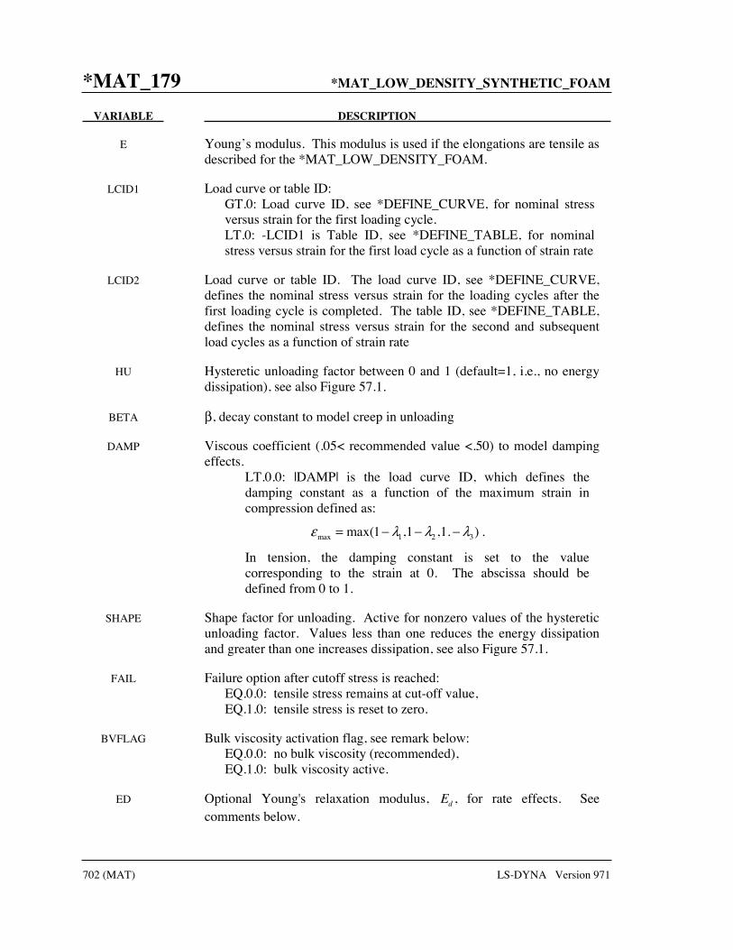
*MAT_179 *MAT_LOW_DENSITY_SYNTHETIC_FOAM
702 (MAT) LS-DYNA Version 971
VARIABLE DESCRIPTION
E Young’s modulus. This modulus is used if the elongations are tensile as described for the *MAT_LOW_DENSITY_FOAM.
LCID1 Load curve or table ID: GT.0: Load curve ID, see *DEFINE_CURVE, for nominal stress
versus strain for the first loading cycle. LT.0: -LCID1 is Table ID, see *DEFINE_TABLE, for nominal
stress versus strain for the first load cycle as a function of strain rate
LCID2 Load curve or table ID. The load curve ID, see *DEFINE_CURVE, defines the nominal stress versus strain for the loading cycles after the first loading cycle is completed. The table ID, see *DEFINE_TABLE, defines the nominal stress versus strain for the second and subsequent load cycles as a function of strain rate
HU Hysteretic unloading factor between 0 and 1 (default=1, i.e., no energy dissipation), see also Figure 57.1.
BETA β, decay constant to model creep in unloading
DAMP Viscous coefficient (.05< recommended value <.50) to model damping effects.
LT.0.0: |DAMP| is the load curve ID, which defines the damping constant as a function of the maximum strain in compression defined as:
max 1 2 3max(1 ,1 ,1. )ε λ λ λ= − − − .
In tension, the damping constant is set to the value corresponding to the strain at 0. The abscissa should be defined from 0 to 1.
SHAPE Shape factor for unloading. Active for nonzero values of the hysteretic unloading factor. Values less than one reduces the energy dissipation and greater than one increases dissipation, see also Figure 57.1.
FAIL Failure option after cutoff stress is reached: EQ.0.0: tensile stress remains at cut-off value, EQ.1.0: tensile stress is reset to zero.
BVFLAG Bulk viscosity activation flag, see remark below: EQ.0.0: no bulk viscosity (recommended), EQ.1.0: bulk viscosity active.
ED Optional Young's relaxation modulus, Ed , for rate effects. See comments below.
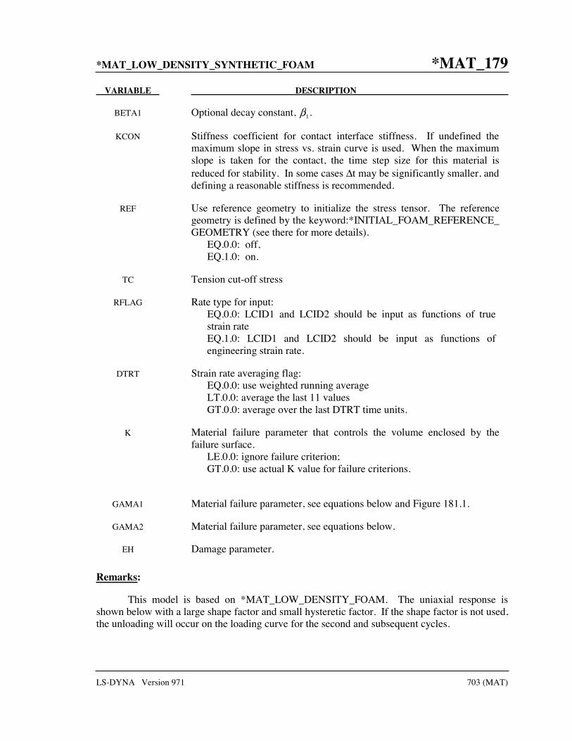
*MAT_LOW_DENSITY_SYNTHETIC_FOAM *MAT_179
LS-DYNA Version 971 703 (MAT)
VARIABLE DESCRIPTION
BETA1 Optional decay constant, β1.
KCON Stiffness coefficient for contact interface stiffness. If undefined the maximum slope in stress vs. strain curve is used. When the maximum slope is taken for the contact, the time step size for this material is reduced for stability. In some cases Δt may be significantly smaller, and defining a reasonable stiffness is recommended.
REF Use reference geometry to initialize the stress tensor. The reference geometry is defined by the keyword:*INITIAL_FOAM_REFERENCE_ GEOMETRY (see there for more details).
EQ.0.0: off, EQ.1.0: on.
TC Tension cut-off stress
RFLAG Rate type for input: EQ.0.0: LCID1 and LCID2 should be input as functions of true
strain rate EQ.1.0: LCID1 and LCID2 should be input as functions of
engineering strain rate.
DTRT Strain rate averaging flag: EQ.0.0: use weighted running average LT.0.0: average the last 11 values GT.0.0: average over the last DTRT time units.
K Material failure parameter that controls the volume enclosed by the failure surface.
LE.0.0: ignore failure criterion; GT.0.0: use actual K value for failure criterions.
GAMA1 Material failure parameter, see equations below and Figure 181.1.
GAMA2 Material failure parameter, see equations below.
EH Damage parameter.
Remarks:
This model is based on *MAT_LOW_DENSITY_FOAM. The uniaxial response is shown below with a large shape factor and small hysteretic factor. If the shape factor is not used, the unloading will occur on the loading curve for the second and subsequent cycles.

*MAT_179 *MAT_LOW_DENSITY_SYNTHETIC_FOAM
704 (MAT) LS-DYNA Version 971
Figure 179.1. Loading and reloading curves.
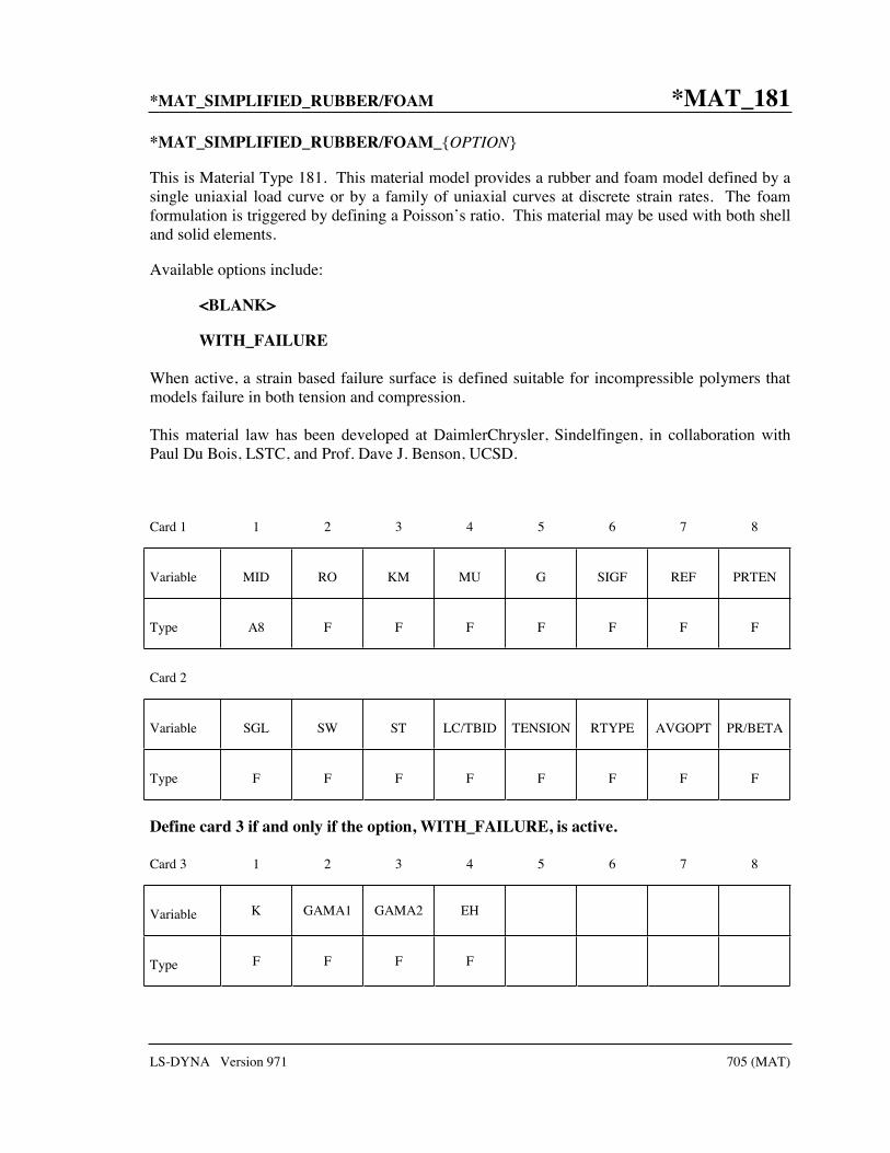
*MAT_SIMPLIFIED_RUBBER/FOAM *MAT_181
LS-DYNA Version 971 705 (MAT)
*MAT_SIMPLIFIED_RUBBER/FOAM_{OPTION}
This is Material Type 181. This material model provides a rubber and foam model defined by a single uniaxial load curve or by a family of uniaxial curves at discrete strain rates. The foam formulation is triggered by defining a Poisson’s ratio. This material may be used with both shell and solid elements.
Available options include:
<BLANK>
WITH_FAILURE
When active, a strain based failure surface is defined suitable for incompressible polymers that models failure in both tension and compression.
This material law has been developed at DaimlerChrysler, Sindelfingen, in collaboration with Paul Du Bois, LSTC, and Prof. Dave J. Benson, UCSD.
Card 1 1 2 3 4 5 6 7 8
Variable MID RO KM MU G SIGF REF PRTEN
Type A8 F F F F F F F
Card 2
Variable SGL SW ST LC/TBID TENSION RTYPE AVGOPT PR/BETA
Type F F F F F F F F
Define card 3 if and only if the option, WITH_FAILURE, is active.
Card 3 1 2 3 4 5 6 7 8
Variable K GAMA1 GAMA2 EH
Type F F F F

*MAT_181 *MAT_SIMPLIFIED_RUBBER/FOAM
706 (MAT) LS-DYNA Version 971
VARIABLE DESCRIPTION
MID Material identification. A unique number or label not exceeding 8 characters must be specified.
RO Mass density
KM Linear bulk modulus.
MU Damping coefficient.
G Shear modulus for frequency independent damping. Frequency independent damping is based of a spring and slider in series. The critical stress for the slider mechanism is SIGF defined below. For the best results, the value of G should be 250-1000 times greater than SIGF.
SIGF Limit stress for frequency independent, frictional, damping.
REF Use reference geometry to initialize the stress tensor. The reference geometry is defined by the keyword:*INITIAL_FOAM_REFERENCE_ GEOMETRY (see there for more details).
EQ.0.0: off, EQ.1.0: on.
PRTEN The tensile Poisson’s ratio for shells (optional). If PRTEN is zero, PR/BETA will serve as the Poisson’s ratio for both tension and compression in shells. If PRTEN is nonzero, PR/BETA will serve only as the compressive Poisson’s ratio for shells.
SGL Specimen gauge length
SW Specimen width
ST Specimen thickness
LC/TBID Load curve or table ID, see *DEFINE_TABLE, defining the force versus actual change in the gauge length. If the table definition is used a family of curves are defined for discrete strain rates. The load curves should cover the complete range of expected loading, i.e., the smallest stretch ratio to the largest. If the first stress-strain curve in the table corresponds to a negative strain rate, LS-DYNA assumes that the natural logarithm of the strain rate value is used. Since the tables are internally discretized to equally space the points, natural logarithms are necessary, for example, if the curves correspond to rates from 10.e-04 to 10.e+04. Computing the natural logarithm of the strain rate does slow the stress update down significantly on some computers.

*MAT_SIMPLIFIED_RUBBER/FOAM *MAT_181
LS-DYNA Version 971 707 (MAT)
VARIABLE DESCRIPTION
TENSION Parameter that controls how the rate effects are treated. Applicable to the table definition.
EQ.-1.0: rate effects are considered during tension and compression loading, but not during unloading,
EQ. 0.0: rate effects are considered for compressive loading only, EQ.1.0: rate effects are treated identically in tension and
compression.
RTYPE Strain rate type if a table is defined: EQ.0.0: true strain rate, EQ.1.0: engineering strain rate
AVGOPT Averaging option determine strain rate to reduce numerical noise. EQ.0.0: simple average of twelve time steps, EQ.1.0: running 12 point average.
PR/BETA If the value is specified between 0 and 0.5 exclusive, i.e.,
0 0.50PR< <
the number defined here is taken as Poisson’s ratio. If zero, an incompressible rubber like behavior is assumed and a default value of 0.495 is used internally. If a Poisson’s ratio of 0.0 is desired, input a small value for PR such as 0.001. When fully integrated solid elements are used and when a nonzero Poisson’s ratio is specified, a foam material is assumed and selective-reduced integration is not used due to the compressibility. This is true even if PR approaches 0.500. If any other value excluding zero is define, then BETA is taken as the absolute value of the given number and a nearly incompressible rubber like behavior is assumed. An incrementally updated mean viscous stress develops according to the equation:
1 1 tn n t
kk
ep p e K where BETA
ββ ε β
β
− ⋅Δ+ − ⋅Δ −= + =
The BETA parameter does not apply to highly compressible foam materials.
K Material failure parameter that controls the volume enclosed by the failure surface.
LE.0.0: ignore failure criterion; GT.0.0: use actual K value for failure criterions.
GAMA1 Material failure parameter, see equations below and Figure 181.1.
GAMA2 Material failure parameter, see equations below.
EH Damage parameter.

*MAT_181 *MAT_SIMPLIFIED_RUBBER/FOAM
708 (MAT) LS-DYNA Version 971
Remarks:
The frequency independent damping is obtained by the having a spring and slider in series as shown in the following sketch:
The general failure criterion for polymers is proposed by Feng and Hallquist as
KIIIIIIf =−Γ+−Γ+−= )3()3()3(),,( 222
111321
where K is a material parameter which controls the size enclosed by the failure surface, and 1I ,
2I and 3I are the three invariants of right Cauchy-Green deformation tensor ( C )
23
22
213
23
22
23
21
22
212
23
22
211
)det(
)CCCC(2
1
C
λλλ
λλλλλλ
λλλ
==
++=−=
++==
CI
I
I
ijijjjii
ii
with iλ are the stretch ratios in three principal directions.
To avoid sudden failure and numerical difficulty, material failure, which is usually a time point, is modeled as a process of damage growth. In this case, the two threshold values are chosen as (1 - h)K and K, where h (also called EH) is a small number chosen based on experimental results reflecting the range between damage initiation and material failure. The damage is defined as function of f :
≥
<<−−+
−≤
=
Kf
KfKhhK
KfKhf
D
if1
)1(if)(
cos12
1)1(if0
π
This definition indicates that damage is first-order continuous. Under this definition, the tangent stiffness matrix will be continuous. The reduced stress considering damage effect is
oijij D σσ )1( −=
where oijσ is the undamaged stress. It is assumed that prior to final failure, material damage is
recoverable. Once material failure occurs, damage will become permanent.

*MAT_SIMPLIFIED_RUBBER/FOAM *MAT_181
LS-DYNA Version 971 709 (MAT)
Figure 181.1. Failure surface for polymer.

*MAT_183 *MAT_SIMPLIFIED_RUBBER_WITH_DAMAGE
710 (MAT) LS-DYNA Version 971
*MAT_SIMPLIFIED_RUBBER_WITH_DAMAGE
This is Material Type 183. This material model provides an incompressible rubber model defined by a single uniaxial load curve for loading (or a table if rate effects are considered) and a single uniaxial load curve for unloading. This model is similar to *MAT_SIMPLIFIED_RUB-BER/FOAM This material may be used with both shell and solid elements.
This material law has been developed at DaimlerChrysler, Sindelfingen, in collaboration with Paul Du Bois, LSTC, and Prof. Dave J. Benson, UCSD.
Card 1 1 2 3 4 5 6 7 8
Variable MID RO K MU G SIGF
Type A8 F F F F F
Card 2
Variable SGL SW ST LCLD TENSION RTYPE AVGOPT
Type F F F F F F F
Card 3
Variable LCUNLD
Type F
VARIABLE DESCRIPTION
MID Material identification. A unique number or label not exceeding 8 characters must be specified.
RO Mass density
K Linear bulk modulus.
MU Damping coefficient.

*MAT_SIMPLIFIED_RUBBER_WITH_DAMAGE *MAT_183
LS-DYNA Version 971 711 (MAT)
VARIABLE DESCRIPTION
G Shear modulus for frequency independent damping. Frequency independent damping is based of a spring and slider in series. The critical stress for the slider mechanism is SIGF defined below. For the best results, the value of G should be 250-1000 times greater than SIGF.
SIGF Limit stress for frequency independent, frictional, damping.
SGL Specimen gauge length
SW Specimen width
ST Specimen thickness
LCLD Load curve, see *DEFINE_CURVE, defining the force versus actual change in the gauge length during loading. The load curve should cover the complete range of expected loading, i.e., the smallest stretch ratio to the largest.
TENSION Parameter that controls how the rate effects are treated. Applicable to the table definition.
EQ.-1.0: rate effects are considered during tension and compression loading, but not during unloading,
EQ. 0.0: rate effects are considered for compressive loading only, EQ.1.0: rate effects are treated identically in tension and
compression.
RTYPE Strain rate type if a table is defined: EQ.0.0: true strain rate, EQ.1.0: engineering strain rate
AVGOPT Averaging option determine strain rate to reduce numerical noise. EQ.0.0: simple average of twelve time steps, EQ.1.0: running 12 point average.
LCUNLD Load curve, see *DEFINE_CURVE, defining the force versus actual change in the gauge length during unloading. The unload curve should cover exactly the same range as LCLD and its end points should have identical values, i.e., the combination of LCLD and LCUNLD describes a complete cycle of loading and unloading.

*MAT_184 *MAT_COHESIVE_ELASTIC
712 (MAT) LS-DYNA Version 971
*MAT_COHESIVE_ELASTIC
This is Material Type 184. It is a simple cohesive elastic model for use with solid element types 19 and 20, and is not available for other solid element formulation. See the remarks after *SECTION_SOLID for a description of element types 19 and 20.
Card 1 1 2 3 4 5 6 7 8
Variable MID RO ROFLG INTFAIL ET EN FN_FAIL
Type A8 F F F F F F
VARIABLE DESCRIPTION
MID Material identification. A unique number or label not exceeding 8 characters must be specified.
RO Mass density
ROFLG Flag for whether density is specified per unit area or volume. ROFLG=0 specified density per unit volume (default), and ROFLG=1 specifies the density is per unit area for controlling the mass of cohesive elements with an initial volume of zero.
INTFAIL The number of integration points required for the cohesive element to be deleted. If it is zero, the element won’t be deleted even if it satisfies the failure criterion. The value of INTFAIL may range from 1 to 4, with 1 the recommended value.
ET The stiffness in the plane of the cohesive element.
EN The stiffness normal to the plane of the cohesive element.
FN_FAIL The force in the normal direction for tensile failure.
Remarks:
This material cohesive model outputs three force resultants into the D3PLOT database rather than the usual six stress components. The in plane shear resultant along the 1-2 edge replaces the x-stress, the orthogonal in plane shear resultant replaces the y-stress, and the normal stress resultant replaces the z-stress.

*MAT_COHESIVE_TH *MAT_185
LS-DYNA Version 971 713 (MAT)
*MAT_COHESIVE_TH
This is Material Type 185. It is a cohesive model by Tvergaard and Hutchinson [1992] for use with solid element types 19 and 20, and is not available for any other solid element formulation. See the remarks after *SECTION_SOLID for a description of element types 19 and 20. The implementation is based on the description of the implementation in the Sandia National Laboratory code, Tahoe [2003].
Card 1 1 2 3 4 5 6 7 8
Variable MID RO ROFLG INTFAIL SIGMAX NLS TLS
Type A8 F F F F F F
Card 2
Variable LAMDA1 LAMDA2 LAMDAF STFSF
Type F F F F
VARIABLE DESCRIPTION
MID Material identification. A unique number or label not exceeding 8 characters must be specified.
RO Mass density
ROFLG Flag for whether density is specified per unit area or volume. ROFLG=0 specified density per unit volume (default), and ROFLG=1 specifies the density is per unit area for controlling the mass of cohesive elements with an initial volume of zero.
INTFAIL The number of integration points required for the cohesive element to be deleted. If it is zero, the element won’t be deleted even if it satisfies the failure criterion. The value of INTFAIL may range from 1 to 4, with 1 the recommended value.
SIGMAX Peak traction.
NLS Length scale (maximum separation) in the normal direction.
TLS Length scale (maximum separation) in the tangential direction.

*MAT_185 *MAT_COHESIVE_TH
714 (MAT) LS-DYNA Version 971
VARIABLE DESCRIPTION
LAMDA1 Scaled distance to peak traction ( 1).
LAMDA2 Scaled distance to beginning of softening ( 2).
LAMDAF Scaled distance for failure ( fail).
STFSF Penetration stiffness multiplier. The penetration stiffness, PS, in terms of input parameters becomes:
*1
*
STFSF SIGMAXPS
LAMDANLS
LAMDAF
=
Remarks:
In this cohesive material model, a dimensionless separation measure is used, which grasps for the interaction between relative displacements in normal ( 3 - mode I) and tangential ( 1, 2 - mode II) directions (see Figure 185.1 left):
22 231 2
TLS TLS NLS
δδ δλ = + +
where the Mc-Cauley bracket is used to distinguish between tension ( 3 0) and compression ( 3<0). NLS and TLS are critical values, representing the maximum separations in the interface in normal and tangential direction. For stress calculation, a trilinear traction-separation law is used, which is given by (see Figure 185.1 right):
( )
11
1 2
22
: //
: / /
1: / 1
1 /
max failfail
max fail fail
max failfail
t
λσ λ
λ σ λλσ λ
< Λ ΛΛ Λ
= Λ Λ < < Λ Λ
− Λ Λ < <− Λ Λ
With these definitions, the traction drops to zero when =1. Then, a potential φ is defined as:
( ) ( )1 2 3
0
, , NLS t dλ
φ δ δ δ λ λ= ⋅
Finally, tangential components (t1, t2) and normal component (t3) of the traction acting on the interface in the fracture process zone are given by:

*MAT_COHESIVE_TH *MAT_185
LS-DYNA Version 971 715 (MAT)
( ) ( )1,2 31,2 3
1,2 3
,t tNLS
t tTLS TLS NLS
δλ λ δφ φδ λ δ λ∂ ∂= = = =
∂ ∂
which in matrix notation is
( )2
2
1 1
2 2
13 3
0 0
0 0
0 0
NLSTLS
NLSTLS
NLS
tt
t
t
δλ
δλ
δ=
In case of compression ( 3<0), penetration is avoided by:
max3 3
1/ fail
STFSFt
NLS
σ δ⋅=⋅Λ Λ
Loading and unloading follows the same path, i.e. this model is completely reversible.
Figure 185.1. Relative displacement and trilinear traction-separation law.
This cohesive material model outputs three force resultants (tractions) into the D3PLOT database rather than the usual six stress components. The in plane shear resultant t1 along the 1-2 edge replaces the x-stress, the orthogonal in plane shear resultant t2 replaces the y-stress, and the normal stress resultant t3 replaces the z-stress.
1
23
maxσ
2/ failΛ Λ 1
λ
( )t λ
1/ failΛ Λ
reversibleloading/unloading

*MAT_186 *MAT_COHESIVE_GENERAL
716 (MAT) LS-DYNA Version 971
*MAT_COHESIVE_GENERAL
This is Material Type 186. This model includes three general irreversible mixed-mode interaction cohesive formulations with arbitrary normalized traction-separation law given by a load curve (TSLC). These three formulations are differentiated via the type of effective separation parameter (TES). The interaction between fracture modes I and II is considered, and irreversible conditions are enforced via a damage formulation (unloading/reloading path pointing to/from the origin). See remarks for details.
Card 1 1 2 3 4 5 6 7 8
Variable MID RO ROFLG INTFAIL TES TSLC GIC GIIC
Type A8 F F F F F F F
Card 2
Variable XMU T S STFSF
Type F F F F
VARIABLE DESCRIPTION
MID Material identification. A unique number or label not exceeding 8 characters must be specified.
RO Mass density.
ROFLG Flag for whether density is specified per unit area or volume. ROFLG=0 specifies density per unit volume (default), and ROFLG=1 specifies the density is per unit area for controlling the mass of cohesive elements with an initial volume of zero.
INTFAIL Number of integration points required for a cohesive element to be deleted. If it is zero, the element won’t be deleted even if it satisfies failure criterion. The value of INTFAIL may range from 1 to 4, with 1 the recommended value.
TES Type of effective separation parameter (ESP). EQ. 0.0 or 1.0: a dimensional separation measure is used. For the
interaction between mode I and II, a mixed-mode propagation criterion is used. For TES=0.0 this is a power-law, and for TES=1.0 this is the Benzeggagh-Kenane law [1996]. See remarks below.

*MAT_COHESIVE_GENERAL *MAT_186
LS-DYNA Version 971 717 (MAT)
VARIABLE DESCRIPTION
EQ. 2.0: a dimensionless separation measure is used, which grasps for the interaction between mode I displacements and mode II displacements (similar to MAT_185, but with damage and general traction-separation law). See remarks below.
TSLC Normalized traction-separation load curve ID. The curve must be normalized in both coordinates and must contain at least three points: (0.0, 0.0), ( 0, 1.0), and (1.0, 0.0), which represents the origin, the peak and the complete failure, respectively (see Figure 186.1). A platform can exist in the curve like the tri-linear TSLC (see MAT_185).
GIC Fracture toughness / energy release rate cIG for mode I
GIIC Fracture toughness / energy release rate cIIG for mode II
XMU Exponent that appears in the power failure criterion (TES=1.0) or the Benzeggagh-Kenane failure criterion (TES=2.0). Recommended values for XMU are between 1.0 and 2.0.
T Peak traction in normal direction (mode I)
S Peak traction in tangential direction (mode II)
STFSF Penetration stiffness multiplier for compression. Factor = (1.0+STFSF) is used to scale the compressive stiffness, i.e. no scaling is done with STFSF=0.0 (recommended).
Remarks:
All three formulations have in common, that the traction-separation behavior of this model is mainly given by c
IG and T for normal mode I, cIIG and S for tangential mode II and an
arbitrary normalized traction-separation load curve for both modes (see Figure 186.1). The maximum (or failure) separations are then given by:
c cF FI III II
TSLC TSLC
G G,
A T A Sδ δ= =
⋅ ⋅
where TSLCA is the area under the normalized traction-separation curve.

*MAT_186 *MAT_COHESIVE_GENERAL
718 (MAT) LS-DYNA Version 971
Figure 186.1. Normalized traction-separation law
For mixed-mode behavior, three different formulations are possible (where default TES=0.0 with XMU=1.0 is recommended as first guess):
First and second formulation (TES=0.0 and TES=1.0)
Here, the total mixed-mode relative displacement mδ is defined as 2 2m I IIδ δ δ= + , where
3Iδ δ= is the separation in normal direction (mode I) and 2 21 2IIδ δ δ= + is the separation in
tangential direction (mode II) (see Figure 186.2). The ultimate mixed-mode displacement Fδ(total failure) for the power law (TES=0.0) is:
1
2 21XMU XMU XMU
Fc c
TSLC I II
T S
A G G
β βδ−
+ ⋅= +
and alternatively for the Benzeggagh-Kenane law [1996] (TES=1.0):
( ) ( )2 2
22
1XMU
F c c cI II I
TSLC
SG G G
T SA T S
β βδββ
+ ⋅= + −+ ⋅+
where /II Iβ δ δ= is the “mode mixity”. The larger the exponent XMU is chosen, the larger the fracture toughness in mixed-mode situations will be. In this model, damage of the interface is considered, i.e. irreversible conditions are enforced with loading/unloading paths coming from/pointing to the origin. This formulation is similar to MAT_COHESIVE_MIXED_MODE (MAT_138), but with the arbitrary traction-separation law TSLC.
F
δλδ
=
max/t t t=
1.0
1.0
TSLCA
mode I mode II
maxt
cG
Fδ
T S
cI
TSLC
G
A T
cIG c
IIG
0λ
possible shape of TSLC
cII
TSLC
G
A S

*MAT_COHESIVE_GENERAL *MAT_186
LS-DYNA Version 971 719 (MAT)
Figure 186.2. Mixed-mode traction-separation law
Third formulation (TES=2.0)Here, a dimensionless effective separation parameter λ is used, which grasps for the interaction between relative displacements in normal ( 3δ - mode I) and tangential ( 1δ , 2δ - mode II)
directions:
2 2 2
31 2F F FII II I
δδ δλδ δ δ
= + +
where the Mc-Cauley bracket is used to distinguish between tension ( 3 0δ ≥ ) and compression
( 3 0δ < ). FIδ and F
IIδ are critical values, representing the maximum separations in the interface
in normal and tangential direction . For stress calculation, the normalized traction-separation load curve TSLC is used: max ( )t t t λ= ⋅ . This formulation is similar to MAT_COHESIVE_TH
(MAT_185), but with the arbitrary traction-separation law and a damage formulation (i.e. irreversible conditions are enforced with loading/unloading paths coming from/pointing to the origin).
Iδ
mδIIδ
ST
1β
Fδ
traction
FIIδ
FIδ
1
23
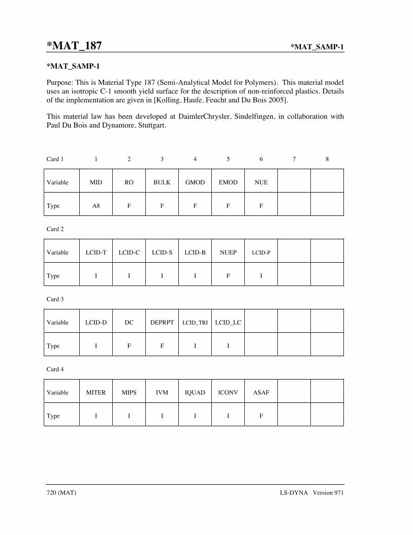
*MAT_187 *MAT_SAMP-1
720 (MAT) LS-DYNA Version 971
*MAT_SAMP-1
Purpose: This is Material Type 187 (Semi-Analytical Model for Polymers). This material model uses an isotropic C-1 smooth yield surface for the description of non-reinforced plastics. Details of the implementation are given in [Kolling, Haufe, Feucht and Du Bois 2005].
This material law has been developed at DaimlerChrysler, Sindelfingen, in collaboration with Paul Du Bois and Dynamore, Stuttgart.
Card 1 1 2 3 4 5 6 7 8
Variable MID RO BULK GMOD EMOD NUE
Type A8 F F F F F
Card 2
Variable LCID-T LCID-C LCID-S LCID-B NUEP LCID-P
Type I I I I F I
Card 3
Variable LCID-D DC DEPRPT LCID_TRI LCID_LC
Type I F F I I
Card 4
Variable MITER MIPS IVM IQUAD ICONV ASAF
Type I I I I I F

*MAT_SAMP-1 *MAT_187
LS-DYNA Version 971 721 (MAT)
VARIABLE DESCRIPTION
MID Material identification. A unique number or label not exceeding 8 characters must be specified.
RO Mass density
BULK Bulk modulus, used by LS-DYNA in the time step calculation
GMOD Shear modulus, used by LS-DYNA in the time step calculation
EMOD Young’s modulus
NUE Poisson ratio
LCID-T Load curve or table ID giving the yield stress as a function of plastic strain, these curves should be obtained from quasi-static and (optionally) dynamic uniaxial tensile tests, this input is mandatory and the material model will not work unless at least one tensile stress-strain curve is given.
LCID-C Load curve ID giving the yield stress as a function of plastic strain, this curve should be obtained from a quasi-static uniaxial compression test, this input is optional.
LCID-S Load curve ID giving the yield stress as a function of plastic strain, this curve should be obtained from a quasi-static shear test, this input is optional.
LCID-B Load curve ID giving the yield stress as a function of plastic strain, this curve should be obtained from a quasi-static biaxial tensile test, this input is optional.
NUEP Plastic Poisson ratio: an estimated ratio of transversal to longitudinal plastic rate of deformation should be given, a value <0 will result in associated plasticity to the yield surface (the associated plasticity option is implemented only for IQUAD=1).
LCID-P Load curve ID giving the plastic Poisson ratio as a function of equivalent plastic deformation during uniaxial tensile testing, if the (optional) load curve is given, the constant value in the previous field will be ignored.
LCID-D Load curve ID giving the damage parameter as a function of equivalent plastic deformation during uniaxial tensile testing, by default this option assumes that effective yield values are used in the load curves LCID-T, LCID-C, LCID-S and LCID-B, if LCID-D is given a negative value, true yield stress values can be used.

*MAT_187 *MAT_SAMP-1
722 (MAT) LS-DYNA Version 971
VARIABLE DESCRIPTION
DC Critical damage value at failure if LCID_D is defined, otherwise, (if LCID-D=0) this parameter is the equivalent plastic strain at failure (EPFAIL). Alternatively, if DC is given as an negative integer, a load curve is expected that defines DC as a function of the plastic strain rate.
DEPRPT Increment of equivalent plastic strain between failure point and rupture point, stresses will fade out to zero between EPFAIL and EPFAIL+DEPRUPT
LCID_TRI Load curve that specifies a factor that works multiplicatively on the value of DC depending on the triaxiality pressure/sigma_vm.. This option is active only if DC is given as a negative value (see above).
LCID_LC Load curve that specifies a factor that works multiplicatively on the value of DC depending on the linear element dimension, this option is active only if DC is given as a negative value (see above).
MITER Maximum number of iterations in the cutting plane algorithm, default is set to 400
MIPS Maximum number of iterations in the secant iteration performed to enforce plane stress (shell elements only), default set to 10
IVM Formulation flag: IVM=0: SAMP-1 formulation (default) IVM=1: vonMises associated plasticity
IQUAD Formulation flag: IQUAD=0: yield surface linear in the vonMises stress (default) IQUAD=1: yield surface quadratic in the vonMises stress
(recommended)
ICONV Formulation flag:ICONV=0: default
ICONV=1: yield surface is internally modified by increasing the shear yield until a convex yield surface is achieved
ICONV=2: if the plastic Poisson ratio is smaller than the elastic Poisson ratio, both are set equal to the smaller value of the two
ASAF Safety factor, used only if ICONV=1, values between 1 and 2 can improve convergence, however the shear yield will be artificially increased if this option is used, default is set to 1.

*MAT_SAMP-1 *MAT_187
LS-DYNA Version 971 723 (MAT)
σ vM
p
σ vM
p
von Mises cylinder
Drucker-Prager cone
Remarks:
Material SAMP-1 uses three yield curves internally, hence the yield surface has a quadratic shape in general. If less than three curves are defined the remaining curves are generated internally as follows:
A linear yield surface in the invariant space spanned by the pressure and the von Mises stress is generated using the available data points.
( )
( )
_ 0
_ 0
_ 0 3
_ 03
_ 02 3_ 0
_ 02
_ 03
_ 0
_ 0
_ 0
_
σ σσσ
σ σσσ σ
σ σσσ σ
= ==
==
=≠ =
−=
≠= =
+=
==
c t
ts
t sc
t s
t cs
t c
LCID C
LCID S
LCID B
LCID C
LCID S
LCID B
LCID C
LCID S
LCID B
LCID C
LCID S
LCID
( )
( )
3 2
03 2
σ σσσ σ
σ σσσ σ
=−
=≠−
t bc
b t
t bs
b t
B

*MAT_187 *MAT_SAMP-1
724 (MAT) LS-DYNA Version 971
SAMP-1 yield surface defined through load
curves
σ vM
p
If more then 2 load curves are available the following cases can be distinguished:
( ) ( )
( )
2
2 2 2
2 2 2
_ 0 1
_ 0
_ 031
_ 02 23
_ 0
_ 06 162
_ 06 323 3
_ 0
_ 0
_ 0
b c ts
b c b t
b s b s t
cb s b t s t
LCID S SAMP
LCID B
LCID C
LCID S
LCID B
LCID C
LCID S
LCID B
LCID C
LCID S
LC
σ σ σσσ σ σ σ
σ σ σ σ σσ
σ σ σ σ σ σ
≠ −=
≠=
+ −≠
= +≠ =
+ +≠
≠≠
_ 0
least squares
ID B ≠
If the LCID_D is given, then a damage curve as a function of equivalent plastic strains acting on the stresses is defined as depicted in the following picture. DC and DEPRPT defined the failure and fading behaviour of a single element:
Figure 187.1
If DC is given as a negative number, its value is calculated via the parameters defined in load curves. In this case the value of
DC = f(LC(strain rate) from |dc|)*f(LCID_TRI(triaxiality))*f(LCID_LC(element length)).
Here the element length is defined as the average of the element diagonals.
d
ε p
εΔ prupt
cd
1.0

*MAT_THERMO_ELASTO_VISCOPLASTIC_CREEP *MAT_188
LS-DYNA Version 971 725 (MAT)
*MAT_THERMO_ELASTO_VISCOPLASTIC_CREEP
This is Material Type 188. In this model, creep is described separately from plasticity using Garafalo’s steady-state hyperbolic sine creep law. Viscous effects of plastic strain rate are considered using the Cowper-Symonds model. Young’s modulus, Poisson’s ratio, thermal expansion coefficient, yield stress, material parameters of Cowper-Symonds model as well as the isotropic and kinematic hardening parameters are all assumed to be temperature dependent. Application scope includes: simulation of solder joints in electronic packaging, modeling of tube brazing process, creep age forming, etc.
Card 1 1 2 3 4 5 6 7 8
Variable MID RO E PR SIGY ALPHA LCSS REFTEM
Type A8 F F F F F F F
Card 2
Variable QR1 CR1 QR2 CR2 QX1 CX1 QX2 CX2
Type F F F F F F F F
Card 3
Variable C P LCE LCPR LCSIGY LCQR LCQX LCALPH
Type F F F F F F F F
Card 4
Variable LCC LCP LCCR LCCX CRPA CRPB CRPQ CRPM
Type F F F F F F F F

*MAT_188 *MAT_THERMO_ELASTO_VISCOPLASTIC_CREEP
726 (MAT) LS-DYNA Version 971
VARIABLE DESCRIPTION
MID Material identification. A unique number or label not exceeding 8 characters must be specified.
RO Mass density.
E Young’s modulus
PR Poisson’s ratio
SIGY Initial yield stress
ALPHA Thermal expansion coefficient
LCSS Load curve ID or Table ID. The load curve ID defines effective stress versus effective plastic strain. The table ID defines for each temperature value a load curve ID giving the stress versus effective plastic strain for that rate. The stress versus effective plastic strain curve for the lowest value of temperature is used if the temperature falls below the minimum value. Likewise, the stress versus effective plastic strain curve for the highest value of temperature is used if the temperature exceeds the maximum value. Card 2 is ignored with this option.
REFTEM Reference temperature that defines thermal expansion coefficient
QR1 Isotropic hardening parameter Qr1
CR1 Isotropic hardening parameter 1rC
QR2 Isotropic hardening parameter 2rQ
CR2 Isotropic hardening parameter Cr2
QX1 Kinematic hardening parameter 1Qχ
CX1 Kinematic hardening parameter 1Cχ
QX2 Kinematic hardening parameter 2Qχ
CX2 Kinematic hardening parameter 2Cχ
C Viscous material parameter C
P Viscous material parameter P
LCE Load curve for scaling Young's modulus as a function of temperature

*MAT_THERMO_ELASTO_VISCOPLASTIC_CREEP *MAT_188
LS-DYNA Version 971 727 (MAT)
VARIABLE DESCRIPTION
LCPR Load curve for scaling Poisson's ratio as a function of temperature
LCSIGY Load curve for scaling initial yield stress as a function of temperature
LCQR Load curve for scaling the isotropic hardening parameters QR1 and QR2 or the stress given by the load curve LCSS as a function of temperature
LCQX Load curve for scaling the kinematic hardening parameters QX1 and QX2 as a function of temperature
LCALPH Load curve for scaling the thermal expansion coefficient as a function of temperature
LCC Load curve for scaling the viscous material parameter C as a function of temperature
LCP Load curve for scaling the viscous material parameter P as a function of temperature
LCCR Load curve for scaling the isotropic hardening parameters CR1 and CR2 as a function of temperature
LCCX Load curve for scaling the isotropic hardening parameters CX1 and CX2 as a function of temperature
CRPA Constant A of Garafalo’s hyperbolic sine creep law (see Remarks)
CRPB Constant B of Garafalo’s hyperbolic sine creep law (see Remarks)
CRPQ Constant Q of Garafalo’s hyperbolic sine creep law (see Remarks)
CRPM Constant m of Garafalo’s hyperbolic sine creep law (see Remarks)
Remarks:
If LCSS is not given any value the uniaxial stress-strain curve has the form
0 1 1 2 2
1 1 2 2
( ) (1 exp( )) (1 exp( ))
(1 exp( )) (1 exp( ))
p p peff r r eff r r eff
p peff eff
Q C Q C
Q C Q Cχ χ χ χ
σ ε σ ε ε
ε ε
= + − − + − −
+ − − + − −
Viscous effects are accounted for using the Cowper-Symonds model, which scales the yield stress with the factor:
1
1pp
eff
C
ε+

*MAT_188 *MAT_THERMO_ELASTO_VISCOPLASTIC_CREEP
728 (MAT) LS-DYNA Version 971
The steady-state creep strain rate of Garafalo’s hyperbolic sine equation is given by
sinh( ) expmc e Q
A BT
ε τ= −

*MAT_ANISOTROPIC_THERMOELASTIC *MAT_189
LS-DYNA Version 971 729 (MAT)
*MAT_ANISOTROPIC_THERMOELASTIC
This is Material Type 189. This model characterizes elastic materials whose elastic properties are temperature-dependent.
Card 1 1 2 3 4 5 6 7 8
Variable MID RO TA1 TA2 TA3 TA4 TA5 TA6
Type A8 F F F F F F F
Card 2
Variable C11 C12 C13 C14 C15 C16 C22 C23
Type F F F F F F F F
Card 3
Variable C24 C25 C26 C33 C34 C35 C36 C44
Type F F F F F F F F
Card 4
Variable C45 C46 C55 C56 C66 TGE TREF AOPT
Type F F F F F F F F
Card 5
Variable XP YP ZP A1 A2 A3 MACF
Type F F F F F F F

*MAT_189 *MAT_ANISOTROPIC_THERMOELASTIC
730 (MAT) LS-DYNA Version 971
Card 6 1 2 3 4 5 6 7 8
Variable V1 V2 V3 D1 D2 D3 BETA REF
Type F F F F F F F F
VARIABLE DESCRIPTION
MID Material identification. A unique number or label not exceeding 8 characters must be specified.
RO Mass density.
TAi Curve IDs defining the coefficients of thermal expansion for the six components of strain tensor as function of temperature.
CIJ Curve IDs defining the 6×6 symmetric constitutive matrix in material coordinate system as function of temperature. Note that 1 corresponds to the a material direction, 2 to the b material direction, and 3 to the cmaterial direction.
TGE Curve ID defining the structural damping coefficient as function of temperature.
TREF Reference temperature for the calculation of thermal loads or the definition of thermal expansion coefficients.
AOPT Material axes option, (see MAT_ANISOTROPIC_ELASTIC/MAT_002 for a complete description.)
EQ.0.0: locally orthotropic with material axes determined by element nodes 1, 2, and 4, as with *DEFINE_COORDINATE_ NODES.
EQ.1.0: locally orthotropic with material axes determined by a point in space and the global location of the element center; this is the a-direction.
EQ.2.0: globally orthotropic with material axes determined by vectors defined below, as with *DEFINE_COORDINATE_ VECTOR.
EQ.3.0: locally orthotropic material axes determined by rotating the material axes about the element normal by an angle, BETA, from a line in the plane of the element defined by the cross product of the vector v with the element normal.
EQ.4.0: locally orthotropic in cylindrical coordinate system with the material axes determined by a vector v, and an originating point, P, which define the centerline axis.

*MAT_ANISOTROPIC_THERMOELASTIC *MAT_189
LS-DYNA Version 971 731 (MAT)
VARIABLE DESCRIPTION
LT.0.0: the absolute value of AOPT is a coordinate system ID number (CID on *DEFINE_COORDINATE_NODES, *DEFINE_ COORDINATE_SYSTEM or *DEFINE_COORDINATE_ VECTOR). Available in R3 version of 971 and later.
XP, YP, ZP XP, YP, ZP define coordinates of point p for AOPT=1 and 4.
A1, A2, A3 a1, a2, a3 define components of vector a for AOPT=2.
MACF Material axis change flag for brick elements (see MAT_002 for a complete description.)
D1, D2, D3 d1, d2, d3 define components of vector d for AOPT=2.
V1, V2, V3 v1, v2, v3 define components of vector v for AOPT=3 and 4.
BETA Material angle in degrees for AOPT=3, may be overwritten on the element card, see *ELEMENT_SHELL_BETA or *ELEMENT_ SOLID_ORTHO.
REF Use initial geometry to initialize the stress tensor (see MAT_002 for a complete description.)

*MAT_190 * MAT_FLD_3-PARAMETER_BARLAT
732 (MAT) LS-DYNA Version 971
*MAT_FLD_3-PARAMETER_BARLAT
This is Material Type 190. This model was developed by Barlat and Lian [1989] for modeling sheets with anisotropic materials under plane stress conditions. This material allows the use of the Lankford parameters for the definition of the anisotropy. This particular development is due to Barlat and Lian [1989]. It has been modified to include a failure criterion based on the Forming Limit Diagram. The curve can be input as a load curve, or calculated based on the n-value and sheet thickness.
Card 1 1 2 3 4 5 6 7 8
Variable MID RO E PR HR P1 P2 ITER
Type A8 F F F F F F F
Card 2
Variable M R00 R45 R90 LCID E0 SPI P3
Type F F F F I F F F
Card 3
Variable AOPT C P FLDCID RN RT FLDSAFE FLDNIPF
Type F F F I F F F I
Card 4
Variable A1 A2 A3
Type F F F

*MAT_FLD_3-PARAMETER_BARLAT *MAT_190
LS-DYNA Version 971 733 (MAT)
Card 5 1 2 3 4 5 6 7 8
Variable V1 V2 V3 D1 D2 D3 BETA
Type F F F F F F F
VARIABLE DESCRIPTION
MID Material identification. A unique number or label not exceeding 8 characters must be specified.
RO Mass density.
E Young’s modulus, E
PR Poisson’s ratio, ν
HR Hardening rule: EQ.1.0: linear (default), EQ.2.0: exponential (Swift) EQ.3.0: load curve EQ.4.0: exponential (Voce) EQ.5.0: exponential (Gosh) EQ.6.0: exponential (Hocket-Sherby)
P1 Material parameter: HR.EQ.1.0: Tangent modulus, HR.EQ.2.0: k, strength coefficient for Swift exponential hardening HR.EQ.4.0: a, coefficient for Voce exponential hardening HR.EQ.5.0: k, strength coefficient for Gosh exponential hardening HR.EQ.6.0: a, coefficient for Hocket-Sherby exponential hardening
P2 Material parameter: HR.EQ.1.0: Yield stress HR.EQ.2.0: n, exponent for Swift exponential hardening HR.EQ.4.0: c, coefficient for Voce exponential hardening HR.EQ.5.0: n, exponent for Gosh exponential hardening HR.EQ.6.0: c. coefficient for Hocket-Sherby exponential hardening
ITER Iteration flag for speed: ITER.EQ.0.0: fully iterative ITER.EQ.1.0: fixed at three iterations Generally, ITER=0 is recommended. However, ITER=1 is somewhat
faster and may give acceptable results in most problems.

*MAT_190 * MAT_FLD_3-PARAMETER_BARLAT
734 (MAT) LS-DYNA Version 971
VARIABLE DESCRIPTION
M m, exponent in Barlat’s yield surface
R00 R00, Lankford parameter determined from experiments
R45 R45, Lankford parameter determined from experiments
R90 R90, Lankford parameter determined from experiments
LCID load curve ID for the load curve hardening rule
E0 Material parameter HR.EQ.2.0: 0ε for determining initial yield stress for Swift
exponential hardening. (Default=0.0) HR.EQ.4.0: b, coefficient for Voce exponential hardening HR.EQ.5.0: 0ε for determining initial yield stress for Gosh
exponential hardening. (Default=0.0) HR.EQ.6.0: b, coefficient for Hocket-Sherby exponential hardening
SPI spi, if 0ε is zero above and HR.EQ.2.0. (Default=0.0)
EQ.0.0: ( ) ( )0 / ** 1/ 1E k nε = −
LE.0.2: 0 spiε = GT.0.2: ( ) [ ]0 / ** 1/spi k nε =
P3 Material parameter: HR.EQ.5.0: p, parameter for Gosh exponential hardening HR.EQ.6.0: n, exponent for Hocket-Sherby exponential hardening
AOPT Material axes option (see MAT_OPTION TROPIC_ELASTIC for a more complete description):
EQ.0.0: locally orthotropic with material axes determined by element nodes 1, 2, and 4, as with *DEFINE_COORDINATE_ NODES.
EQ.2.0: globally orthotropic with material axes determined by vectors defined below, as with *DEFINE_COORDINATE_ VECTOR.
EQ.3.0: locally orthotropic material axes determined by rotating the material axes about the element normal by an angle, BETA, from a line in the plane of the element defined by the cross product of the vector v with the element normal.
LT.0.0: the absolute value of AOPT is a coordinate system ID number (CID on *DEFINE_COORDINATE_NODES, *DEFINE_ COORDINATE_SYSTEM or *DEFINE_COORDINATE_ VECTOR). Available in R3 version of 971 and later.

*MAT_FLD_3-PARAMETER_BARLAT *MAT_190
LS-DYNA Version 971 735 (MAT)
VARIABLE DESCRIPTION
C C in Cowper-Symonds strain rate model
P p in Cowper-Symonds strain rate model, p=0.0 for no strain rate effects
FLDCID Load curve ID defining the Forming Limit Diagram. Minor strains in percent are defined as abscissa values and Major strains in percent are defined as ordinate values. The forming limit diagram is shown in Figure 39.1. In defining the curve list pairs of minor and major strains starting with the left most point and ending with the right most point, see *DEFINE_CURVE.
RN Hardening exponent equivalent to the n-value in a power law hardening law. If the parameter FLDCID is not defined, this value in combination with the value RT can be used to calculate a forming limit curve to allow for failure.
RT Sheet thickness used for calculating a forming limit curve. This value does not override the sheet thickness in any way. It is only used in conjunction with the parameter RN to calculate a forming limit curve if the parameter FLDCID is not defined.
FLDSAFE A safety offset of the forming limit curve. This value should be input as a percentage (ex. 10 not 0.10). This safety margin will be applied to the forming limit curve defined by FLDCID or the curve calculated by RN and RT.
FLDNIPF The number of element integration points that must fail before the element is deleted. By default, if one integration point has strains above the forming limit curve, the element is flagged for deletion.
A1 A2 A3 Components of vector a for AOPT = 2.
V1 V2 V3 Components of vector v for AOPT = 3.
D1 D2 D3 Components of vector d for AOPT = 2.
BETA Material angle in degrees for AOPT = 3, may be overridden on the element card, see *ELEMENT_SHELL_BETA.
Remarks:
See material 36 for the theoretical basis.
The forming limit curve can be input directly as a curve by specifying a load curve id with the parameter FLDCID. When defining such a curve, the major and minor strains must be input as percentages.

*MAT_190 * MAT_FLD_3-PARAMETER_BARLAT
736 (MAT) LS-DYNA Version 971
Alternatively, the parameters RN and RT can be used to calculate a forming limit curve. The use of RN and RT is not recommended for non-ferrous materials. RN and RT are ignored if a non-zero FLDCID is defined.
The first history variable is the maximum strain ratio defined by:
workpiece
fld
major
major
εε
corresponding to minorworkpieceε . A value between 0 and 1 indicates that the strains lie below the
forming limit curve. Values above 1 indicate that the strains are above the forming limit curve.

*MAT_SEISMIC_BEAM *MAT_191
LS-DYNA Version 971 737 (MAT)
*MAT_SEISMIC_BEAM
Purpose: This is Material Type 191. This material enables lumped plasticity to be developed at the ‘node 2’ end of Belytschko-Schwer beams (resultant formulation). The plastic yield surface allows interaction between the two moments and the axial force.
Note: The following options will be available in release 3 of version 971: DEGRAD, IFEMA,FOFFS, FEMAi.
Card 1 1 2 3 4 5 6 7 8
Variable MID RO E PR AOPT FTYPE DEGRAD IFEMA
Type A8 F F F F I I I
Default none none none none 0.1 1 0 0
Card 2
Variable LCPMS SFS LCPMT SFT LCAT SFAT LCAC SFAC
Type F F F F F F F F
Default none 1.0 LCMPS 1.0 none 1.0 LCAT 1.0
Define the following card for interaction formulation, FTYPE, type 1 (Default)
Card 3 1 2 3 4 5 6 7 8
Variable ALPHA BETA GAMMA DELTA A B FOFFS
Type F F F F F F F
Default see note see note see note see note see note see note 0.0

*MAT_191 *MAT_SEISMIC_BEAM
738 (MAT) LS-DYNA Version 971
Define the following card for interaction formulation, FTYPE, type 2
Card 3 1 2 3 4 5 6 7 8
Variable SIGY D W TF TW
Type F F F F F
Default none none none none none
Define the following card for FEMA limits only if IFEMA > 0
Card 4 1 2 3 4 5 6 7 8
Variable PR1 PR2 PR3 PR4
Type F F F F
Default 0 0 0 0
Define the following card for FEMA limits only if IFEMA = 2
Card 4 1 2 3 4 5 6 7 8
Variable TS1 TS2 TS3 TS4 CS1 CS2 CS3 CS4
Type F F F F F F F F
Default 0 0 0 0 =TS1 =TS2 =TS3 =TS4
VARIABLE DESCRIPTION
MID Material identification. A unique number or label not exceeding 8 characters must be specified.
RO Mass density.
E Young’s modulus.
PR Poisson’s ratio.

*MAT_SEISMIC_BEAM *MAT_191
LS-DYNA Version 971 739 (MAT)
VARIABLE DESCRIPTION
AOPT Axial force option EQ.0.0: Axial load curves are collapse load vs. strain EQ.1.0: Axial load curves are collapse load vs. change in length EQ.2.0: Axial load curves are collapse load vs. nominal total strain
(“total strain” is elastic+plastic strains) LT.0.0: the absolute value of AOPT is a coordinate system ID
number (CID on *DEFINE_COORDINATE_NODES, *DEFINE_ COORDINATE_SYSTEM or *DEFINE_COORDINATE_ VECTOR). Available in R3 version of 971 and later.
FTYPE Formulation type for interaction EQ.1: Parabolic coefficients, axial load and biaxial bending
(default). EQ.2: Japanese code, axial force and major axis bending.
DEGRADE Flag for degrading moment behavior (see Remarks) EQ.0: Behavior as in previous versions EQ.1: Fatigue-type degrading moment-rotation behavior EQ.2: FEMA-type degrading moment-rotation behavior
IFEMA Flag for input of FEMA thresholds EQ.0: No input EQ.1: Input of rotation thresholds only EQ.2: Input of rotation and axial strain thresholds
LCPMS Load curve ID giving plastic moment vs. Plastic rotation at node 2 about local s-axis. See *DEFINE_CURVE.
SFS Scale factor on s-moment at node 2.
LCPMT Load curve ID giving plastic moment vs. Plastic rotation at node 2 about local t-axis. See *DEFINE_CURVE.
SFT Scale factor on t-moment at node 2.
LCAT Load curve ID giving axial tensile yield force vs. total tensile (elastic + plastic) strain or vs. elongation. See AOPT above. All values are positive. See *DEFINE_CURVE.
SFAT Scale factor on axial tensile force.
LCAC Load curve ID giving compressive yield force vs. total compressive (elastic + plastic) strain or vs. elongation. See AOPT above. All values are positive. See *DEFINE_CURVE.
SFAC Scale factor on axial tensile force.
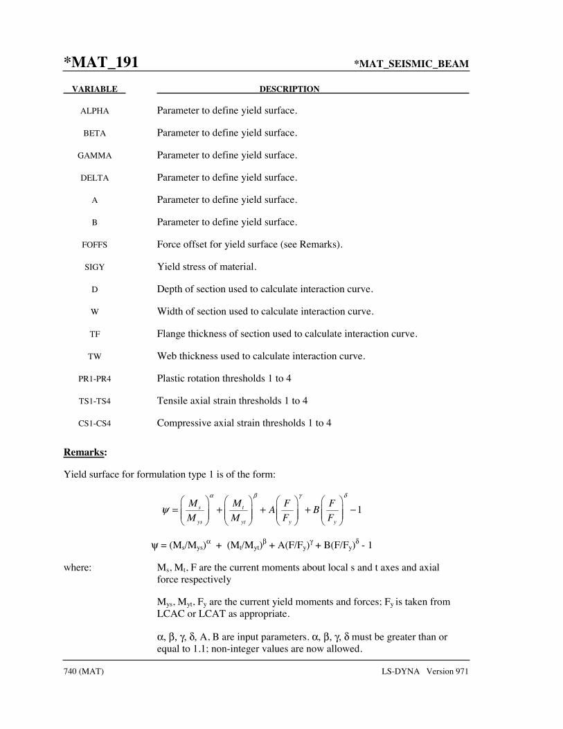
*MAT_191 *MAT_SEISMIC_BEAM
740 (MAT) LS-DYNA Version 971
VARIABLE DESCRIPTION
ALPHA Parameter to define yield surface.
BETA Parameter to define yield surface.
GAMMA Parameter to define yield surface.
DELTA Parameter to define yield surface.
A Parameter to define yield surface.
B Parameter to define yield surface.
FOFFS Force offset for yield surface (see Remarks).
SIGY Yield stress of material.
D Depth of section used to calculate interaction curve.
W Width of section used to calculate interaction curve.
TF Flange thickness of section used to calculate interaction curve.
TW Web thickness used to calculate interaction curve.
PR1-PR4 Plastic rotation thresholds 1 to 4
TS1-TS4 Tensile axial strain thresholds 1 to 4
CS1-CS4 Compressive axial strain thresholds 1 to 4
Remarks:
Yield surface for formulation type 1 is of the form:
1s t
ys yt y y
M M F FA B
M M F F
α β γ δ
ψ = + + + −
ψ = (Ms/Mys)α + (Mt/Myt)
β + A(F/Fy)γ + B(F/Fy)
δ - 1
where: Ms, Mt, F are the current moments about local s and t axes and axial force respectively
Mys, Myt, Fy are the current yield moments and forces; Fy is taken from LCAC or LCAT as appropriate.
α, β, γ, δ, A, B are input parameters. α, β, γ, δ must be greater than or equal to 1.1; non-integer values are now allowed.

*MAT_SEISMIC_BEAM *MAT_191
LS-DYNA Version 971 741 (MAT)
If α, β, γ, δ, A and B are all set to zero then the following default values are used:
ALPHA = 2.0 BETA = 2.0 GAMMA = 2.0 DELTA = 4.0 A = 2.0 B = -1.0
FOFFS offsets the yield surface parallel to the axial force axis. It is the compressive axial force at which the maximum bending moment capacity about the local s-axis (determined by LCPMS and SFS), and that about the local t-axis (determined by LCPMT and SFT), occur. For steel beams and columns, the value of FOFFS is usually zero. For reinforce concrete beams, columns and shear walls, the maximum bending moment capacity occurs corresponding to a certain compressive axial force, FOFFS. The value of FOFFS can be input as either positive or negative. Internally, LS-DYNA converts FOFFS to, and regards compressive axial force as, negative.
The option for degrading moment behavior changes the meaning of the plastic moment-rotation curve as follows:
If DEGRAD=0, the x-axis points on the curve represent current plastic rotation (i.e. total rotation minus the elastic component of rotation). This quantity can be positive or negative depending on the direction of rotation; during hysteresis the behavior will repeatedly follow backwards and forwards along the same curve. The curve should include negative and positive rotation and moment values. This option is retained so that results from existing models will be unchanged.
If DEGRAD=1, the x-axis points represent cumulative absolute plastic rotation. This quantity is always positive, and increases whenever there is plastic rotation in either direction. Thus, during hysteresis, the yield moments are taken from points in the input curve with increasingly positive rotation. If the curve shows a degrading behavior (reducing moment with rotation), then, once degraded by plastic rotation, the yield moment can never recover to its initial value. This option can be thought of as having “fatigue-type” hysteretic damage behavior, where all plastic cycles contribute to the total damage.
If DEGRAD=2, the x-axis points represent the high-tide value (always positive) of the plastic rotation. This quantity increases only when the absolute value of plastic rotation exceeds the previously recorded maximum. If smaller cycles follow a larger cycle, the plastic moment during the small cycles will be constant, since the high-tide plastic rotation is not altered by the small cycles. Degrading moment-rotation behavior is possible. This option can be thought of as showing rotation-controlled damage, and follows the FEMA approach for treating fracturing joints.
DEGRAD applies also to the axial behavior. The same options are available as for rotation: DEGRAD=0 gives unchanged behavior from previous versions; DEGRAD=1 gives a fatigue-type behavior using cumulative plastic strain; and DEGRAD=2 gives FEMA-type behavior, where the axial load capacity depends on the high-tide tensile and compressive strains. The definition of strain for this purpose is according to AOPT on Card 1 – it is expected that

*MAT_191 *MAT_SEISMIC_BEAM
742 (MAT) LS-DYNA Version 971
AOPT=2 will be used with DEGRAD=2. The “axial strain” variable plotted by post-processors is the variable defined by AOPT.
The output variables plotted as “plastic rotation” have special meanings for this material model as follows – note that hinges form only at Node 2:
“Plastic rotation at End 1” is really a high-tide mark of absolute plastic rotation at Node 2,defined as follows:
1. Current plastic rotation is the total rotation minus the elastic component of rotation. 2. Take the absolute value of the current plastic rotation, and record the maximum
achieved up to the current time. This is the high-tide mark of plastic rotation.
If DEGRAD=0, “Plastic rotation at End 2” is the current plastic rotation at Node 2.
If DEGRAD=1 or 2, “Plastic rotation at End 2” is the current total rotation at Node 2.
The total rotation is a more intuitively understood parameter, e.g. for plotting hysteresis loops. However, with DEGRAD=0, the previous meaning of that output variable has been retained such that results from existing models are unchanged.
FEMA thresholds are the plastic rotations at which the element is deemed to have passed from one category to the next, e.g. “Elastic”, “Immediate Occupancy”, “Life Safe”, etc. The high-tide plastic rotation (maximum of Y and Z) is checked against the user-defined limits FEMA1, FEMA2, etc. The output flag is then set to 0, 1, 2, 3, or 4: 0 means that the rotation is less than FEMA1; 1 means that the rotation is between FEMA1 and FEMA2, and so on. By contouring this flag, it is possible to see quickly which joints have passed critical thresholds.
For this material model, special output parameters are written to the d3plot and d3thdt files. The number of output parameters for beam elements is automatically increased to 20 (in addition to the six standard resultants) when parts of this material type are present. Some post-processors may interpret this data as if the elements were integrated beams with 4 integration points. Depending on the post-processor used, the data may be accessed as follows:
Extra variable 16 (or Integration point 4 Axial Stress): FEMA rotation flag Extra variable 17 (or Integration point 4 XY Shear Stress): Current utilization Extra variable 18 (or Integration point 4 ZX Shear Stress): Maximum utilization to date Extra variable 20 (or Integration point 4 Axial Strain): FEMA axial flag
“Utilization” is the yield parameter, where 1.0 is on the yield surface.

*MAT_SOIL_BRICK *MAT_192
LS-DYNA Version 971 743 (MAT)
*MAT_SOIL_BRICK
Purpose: This is Material Type 192. It is intended for modeling over-consolidated clay.
Card 1 1 2 3 4 5 6 7 8
Variable MID RO RLAMDA RKAPPA RIOTA RBETA1 RBETA2 RMU
Type A8 F F F F F F F
Default 1.0
Card 2
Variable RNU RLCID TOL PGCL SUB-INC BLK GRAV THEORY
Type F F F F F F F I
Default 0.0005 9.807 0
Define Card 3 only if THEORY>0
Card 3 1 2 3 4 5 6 7 8
Variable RVHHH XSICRIT ALPHA RVH RNU21 ANISO_4
Type F F F F F F
Default 0 0 0 0 0 0
VARIABLE DESCRIPTION
MID Material identification. A unique number or label not exceeding 8 characters must be specified.
RO Mass density
RLAMDA Material coefficient

*MAT_192 *MAT_SOIL_BRICK
744 (MAT) LS-DYNA Version 971
VARIABLE DESCRIPTION
RKAPPA Material coefficient
RIOTA Material coefficient
RBETA1 Material coefficient
RBETA2 Material coefficient
RMU Shape factor coefficient. This parameter will modify the shape of the yield surface used. 1.0 implies a von Mises type surface, but 1.1 to 1.25 is more indicative of soils. The default value is 1.0.
RNU Poisson’s ratio
RLCID Load curve identification number referring to a curve defining up to 10 pairs of ‘string-length’ vs G/Gmax points.
TOL User defined tolerance for convergence checking. Default value is set to 0.02.
PGCL Pre-consolidation ground level. This parameter defines the maximum surface level (relative to z = 0.0 in the model) of the soil throughout geological history. This is used calculate the maximum over burden pressure on the soil elements.
SUB-INC User defined strain increment size. This is the maximum strain increment that the material model can normally cope with. If the value is exceeded a warning is echoed to the d3hsp file.
BLK The elastic bulk stiffness of the soil. This is used for the contact stiffness only.
GRAV The gravitational acceleration. This is used to calculate the element stresses due the overlying soil. Default is set to 9.807 m/s2.
THEORY Version of material subroutines used (See Remarks). EQ. 0: 1995 version, vectorized (Default) EQ. 4: 2003 version, unvectorized
RVHHH Anisotropy ratio Gvh / Ghh (default = Isotropic behavior)
XSICRIT Anisotropy parameter
ALPHA Anisotropy parameter
RVH Anisotropy ratio Ev / Eh
RNU21 Anisotropy ratio 2 1/ν ν
ANISO_4 Anisotropy parameter

*MAT_SOIL_BRICK *MAT_192
LS-DYNA Version 971 745 (MAT)
Remarks:
1. This material type requires that the model is oriented such that the z-axis is defined in the upward direction. Compressive initial stress must be defined, e.g. using *INITIAL_STRESS_SOLID or *INITIAL_STRESS_DEPTH. The recommended unit system is kN, meters, seconds, tonnes. There are some built-in defaults that assume stress units of KN/m2.
Over-consolidated clays have suffered previous loading to higher stress levels than are present at the start of the analysis. This could have occurred due to ice sheets during previous ice ages, or the presence of soil or rock that has subsequently been eroded. The maximum vertical stress during that time is assumed to be:
σVMAX = RO*GRAV*(PGCL – Zel)
whereRO, GRAV, PGCL = input parameters Zel = z-coordinate of center of element
Since that time, the material has been unloaded until the vertical stress equals the user-defined initial vertical stress. The previous load/unload history has a significant effect on subsequent behavior, e.g. the horizontal stress in an over-consolidated clay may be greater than the vertical stress.
This material model creates a load/unload cycle for a sample element of each material of this type, stores in a scratch file the horizontal stress and history variables as a function of the vertical stress, and interpolates these quantities from the defined initial vertical stress for each element. Therefore the initial horizontal stress seen in the output files will be different from the input initial horizontal stress.
This material model is developed for a Geotechnical FE program (Oasys SAFE) written by Arup. The default THEORY=0 gives a vectorized version ported from SAFE in the 1990’s. Since then the material model has been developed further in SAFE; the most recent porting is accessed using THEORY=4 (recommended); however, this version is not vectorized and will run more slowly on most computer platforms.
2. The shape factor for a typical soil would be 1.25. Do not use values higher than 1.35.

*MAT_193 *MAT_DRUCKER_PRAGER
746 (MAT) LS-DYNA Version 971
*MAT_DRUCKER_PRAGER
Purpose: This is Material Type 193. This material enables soil to be modeled effectively. The parameters used to define the yield surface are familiar geotechnical parameters (i.e. angle of friction). The modified Drucker-Prager yield surface is used in this material model enabling the shape of the surface to be distorted into a more realistic definition for soils.
Card 1 1 2 3 4 5 6 7 8
Variable MID RO GMOD RNU RKF PHI CVAL PSI
Type A8 F F F F F F F
Default 1.0 0.0
Card 2
Variable STR_LIM
Type F
Default 0.005
Card 3
Variable GMODDP PHIDP CVALDP PSIDP GMODGR PHIGR CVALGR PSIGR
Type F F F F F F F F
Default 0.0 0.0 0.0 0.0 0.0 0.0 0.0 0.0
VARIABLE DESCRIPTION
MID Material identification. A unique number or label not exceeding 8 characters must be specified.
RO Mass density

*MAT_DRUCKER_PRAGER *MAT_193
LS-DYNA Version 971 747 (MAT)
VARIABLE DESCRIPTION
GMOD Elastic shear modulus
RNU Poisson’s ratio
RKF Failure surface shape parameter
PHI Angle of friction (radians)
CVAL Cohesion value
PSI Dilation angle (radians)
STR_LIM Minimum shear strength of material is given by STR_LIM*CVAL
GMODDP Depth at which shear modulus (GMOD) is correct
PHIDP Depth at which angle of friction (PHI) is correct
CVALDP Depth at which cohesion value (CVAL) is correct
PSIDP Depth at which dilation angle (PSI) is correct
GMODGR Gradient at which shear modulus (GMOD) increases with depth
PHIGR Gradient at which friction angle (PHI) increases with depth
CVALGR Gradient at which cohesion value (CVAL) increases with depth
PSIGR Gradient at which dilation angle (PSI) increases with depth
Remarks:
1. This material type requires that the model is oriented such that the z-axis is defined in the upward direction. The key parameters are defined such that may vary with depth (i.e. the z-axis).
2. The shape factor for a typical soil would be 0.8, but should not be pushed further than 0.75.
3. If STR_LIM is set to less than 0.005, the value is reset to 0.005.

*MAT_194 *MAT_RC_SHEAR_WALL
748 (MAT) LS-DYNA Version 971
*MAT_RC_SHEAR_WALL
Purpose: This is Material Type 194. It is for shell elements only. It uses empirically-derived algorithms to model the effect of cyclic shear loading on reinforced concrete walls. It is primarily intended for modeling squat shear walls, but can also be used for slabs. Because the combined effect of concrete and reinforcement is included in the empirical data, crude meshes can be used. The model has been designed such that the minimum amount of input is needed: generally, only the variables on the first card need to be defined.
Card 1 1 2 3 4 5 6 7 8
Variable MID RO E PR TMAX I
Type A8 F F F F
Default none none none 0.0 0.0
Define the following data if “Uniform Building Code” formula for maximum shear strength or tensile cracking are required – otherwise leave blank.
Card 2 1 2 3 4 5 6 7 8
Variable FC PREF FYIELD SIG0 UNCONV ALPHA FT ERIENF
Type F F F F F F F F
Default 0.0 0.0 0.0 0.0 0.0 0.0 0.0 0.0
Card 3
Variable A B C D E F
Type F F F F F F
Default 0.05 0.55 0.125 0.66 0.25 1.0

*MAT_RC_SHEAR_WALL *MAT_194
LS-DYNA Version 971 749 (MAT)
Card 4 1 2 3 4 5 6 7 8
Variable Y1 Y2 Y3 Y4 Y5
Type F F F F F
Default 0.0 0.0 0.0 0.0 0.0
Card 5
Variable T1 T2 T3 T4 T5
Type F F F F F
Default 0.0 0.0 0.0 0.0 0.0
Card 6
Variable AOPT
Type F
Default 0.0
Card 7
Variable XP YP ZP A1 A2 A3
Type F F F F F F
Default 0.0 0.0 0.0 0.0 0.0 0.0

*MAT_194 *MAT_RC_SHEAR_WALL
750 (MAT) LS-DYNA Version 971
Card 8 1 2 3 4 5 6 7 8
Variable V1 V2 V3 D1 D2 D3 BETA
Type F F F F F F F
Default 0.0 0.0 0.0 0.0 0.0 0.0 0.0
VARIABLE DESCRIPTION
MID Material identification. A unique number or label not exceeding 8 characters must be specified.
RO Mass density
E Young’s Modulus
PR Poisson’s Ratio
TMAX Ultimate in-plane shear stress. If set to zero, LS-DYNA will calculate TMAX based on the formulae in the Universal Building Code, using the data on card 2. See Remarks.
FC Unconfined Compressive Strength of concrete (used in the calculation of ultimate shear stress; crushing behavior is not modeled)
PREF Percent reinforcement, e.g. if 1.2% reinforcement, enter 1.2
FYIELD Yield stress of reinforcement
SIG0 Overburden stress (in-plane compressive stress) - used in the calculation of ultimate shear stress. Usually sig0 is left as zero.
UCONV Unit conversion factor. UCONV = (1.0 psi in the model stress units). This is needed because the ultimate tensile stress of concrete is expressed as (FC) where FC is in psi. Therefore a unit conversion factor of (psi/stress unit) is required. Examples:
UCONV = 0.083 if stress unit is MN/m2 or N/mm2
UCONV = 83.3 if stress unit is N/m2
ALPHA Shear span factor - see below.
FT Cracking stress in direct tension - see notes below. Default is 8% of the cylinder strength.

*MAT_RC_SHEAR_WALL *MAT_194
LS-DYNA Version 971 751 (MAT)
VARIABLE DESCRIPTION
ERIENF Young’s Modulus of reinforcement. Used in calculation of post-cracked stiffness - see notes below.
A Hysteresis constants determining the shape of the hysteresis loops.
B Hysteresis constants determining the shape of the hysteresis loops.
C Hysteresis constants determining the shape of the hysteresis loops.
D Hysteresis constants determining the shape of the hysteresis loops.
E Hysteresis constants determining the shape of the hysteresis loops.
F Strength degradation factor. After the ultimate shear stress has been achieved, F multiplies the maximum shear stress from the curve for subsequent reloading. F=1.0 implies no strength degradation (default). F=0.5 implies that the strength is halved for subsequent reloading.
Y1,Y2...Y5 Shear strain points on stress-strain curve. By default these are calculated from the values on card 1. See below for more guidance.
T1,T2...T5 Shear stress points on stress-strain curve. By default these are calculated from the values on card 1. See below for more guidance.
AOPT Material axes option: EQ. 0.0: locally orthotropic with material axes determined by
element nodes as shown in Figure 2.1. Nodes 1, 2, and 4 of an element are identical to the Nodes used for the definition of a coordinate system as by *DEFINE_COORDINATE_NODES.
EQ. 2.0: globally orthotropic with material axes determined by vectors defined below, as with *DEFINE_COORDINATE_ VECTOR.
EQ. 3.0: applicable to shell elements only. This option determines locally orthotropic material axes by offsetting the material axes by an angle to be specified from a line in the plane of the shell determined by taking the cross product of the vector v defined below with the shell normal vector.
LT.0.0: the absolute value of AOPT is a coordinate system ID number (CID on *DEFINE_COORDINATE_NODES, *DEFINE_ COORDINATE_SYSTEM or *DEFINE_COORDINATE_ VECTOR). Available in R3 version of 971 and later.
XP,YP,ZP Coordinates of point p for AOPT = 1.
A1,A2,A3 Components of vector a for AOPT = 2.
V1,V2,V3 Components of vector v for AOPT = 3.
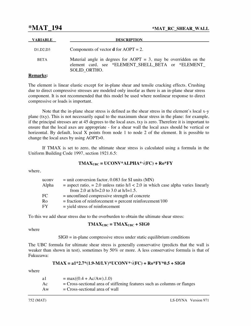
*MAT_194 *MAT_RC_SHEAR_WALL
752 (MAT) LS-DYNA Version 971
VARIABLE DESCRIPTION
D1,D2,D3 Components of vector d for AOPT = 2.
BETA Material angle in degrees for AOPT = 3, may be overridden on the element card, see *ELEMENT_SHELL_BETA or *ELEMENT_ SOLID_ORTHO.
Remarks:
The element is linear elastic except for in-plane shear and tensile cracking effects. Crushing due to direct compressive stresses are modeled only insofar as there is an in-plane shear stress component. It is not recommended that this model be used where nonlinear response to direct compressive or loads is important.
Note that the in-plane shear stress is defined as the shear stress in the element’s local x-y plane (txy). This is not necessarily equal to the maximum shear stress in the plane: for example, if the principal stresses are at 45 degrees to the local axes, txy is zero. Therefore it is important to ensure that the local axes are appropriate - for a shear wall the local axes should be vertical or horizontal. By default, local X points from node 1 to node 2 of the element. It is possible to change the local axes by using AOPT>0.
If TMAX is set to zero, the ultimate shear stress is calculated using a formula in the Uniform Building Code 1997, section 1921.6.5:
TMAXUBC = UCONV*ALPHA* (FC) + Ro*FY
where,
uconv = unit conversion factor, 0.083 for SI units (MN) Alpha = aspect ratio, = 2.0 unless ratio h/l < 2.0 in which case alpha varies linearly
from 2.0 at h/l=2.0 to 3.0 at h/l=1.5. FC = unconfined compressive strength of concrete Ro = fraction of reinforcement = percent reinforcement/100 FY = yield stress of reinforcement
To this we add shear stress due to the overburden to obtain the ultimate shear stress:
TMAXUBC = TMAXUBC + SIG0 where
SIG0 = in-plane compressive stress under static equilibrium conditions
The UBC formula for ultimate shear stress is generally conservative (predicts that the wall is weaker than shown in test), sometimes by 50% or more. A less conservative formula is that of Fukuzawa:
TMAX = a1*2.7*(1.9-M/LV)*UCONV* (FC) + Ro*FY*0.5 + SIG0
where
a1 = max((0.4 + Ac/Aw),1.0) Ac = Cross-sectional area of stiffening features such as columns or flanges Aw = Cross-sectional area of wall

*MAT_RC_SHEAR_WALL *MAT_194
LS-DYNA Version 971 753 (MAT)
M/LV = Aspect ratio of wall (height/length)
Other terms are as above. This formula is not included in the material model: TMAX should be calculated by hand and entered on Card 1 if the Fukuzawa formula is required.
It should be noted that none of the available formulae, including Fukuzawa, predict the ultimate shear stress accurately for all situations. Variance from the experimental results can be as great as 50%.
The shear stress vs shear strain curve is then constructed automatically as follows, using the algorithm of Fukuzawa extended by Arup:
Assume ultimate shear strain, γu = 0.0048
First point on curve (concrete cracking) at (0.3TMAX/G, 0.3TMAX) where G is the elastic shear modulus given by E/2(1+v)
Second point (reinforcement yield) at (0.5γu, 0.8TMAX)
Third point (ultimate strength) at (γu, TMAX)
Fourth point (onset of strength reduction) at (2γu, TMAX)
Fifth point (failure) at (3γu, 0.6TMAX).
After failure, the shear stress drops to zero. The curve points can be entered by the user if desired, in which case they over-ride the automatically calculated curve. However, it is anticipated that in most cases the default curve will be preferred due to ease of input.
Hysteresis follows the algorithm of Shiga as for the squat shear wall spring (see *MAT_SPRING_SQUAT_SHEARWALL). The hysteresis constants A,B,C,D,E can be entered by the user if desired but it is generally recommended that the default values be used.
Cracking in tension is checked for the local x and y directions only – this is calculated separately from the in-plane shear. A trilinear response is assumed, with turning points at concrete cracking and reinforcement yielding. The three regimes are:
1. Pre-cracking, linear elastic response is assumed using the overall Young’s Modulus on Card 1.
2. Cracking occurs in the local x or y directions when the tensile stress in that direction exceeds the concrete tensile strength FT (if not input on Card 2, this defaults to 8% of the compressive strength FC). Post-cracking, a linear stress-strain response is assumed up to reinforcement yield at a strain defined by reinforcement yield stress divided by reinforcement Young’s Modulus.
3. Post-yield, a constant stress is assumed (no work hardening).
Unloading returns to the origin of the stress-strain curve.
For compressive strains the response is always linear elastic using the overall Young’s Modulus on Card 1.

*MAT_194 *MAT_RC_SHEAR_WALL
754 (MAT) LS-DYNA Version 971
If insufficient data is entered, no cracking occurs in the model. As a minimum, FC and FY are needed.
Extra variables are available for post-processing as follows:
Extra variable 1: Current shear strain Extra variable 2: Shear status: 0,1,2,3,4 or 5– see below Extra variable 3: Maximum direct strain so far in local X direction (for tensile cracking) Extra variable 4: Maximum direct strain so far in local Y direction (for tensile cracking) Extra variable 5: Tensile status: 0,1 or 2 = elastic, cracked, or yielded respectively.
The shear status shows how far along the shear stress-strain curve each element has progressed, e.g. status 2 means that the element has passed the second point on the curve. These status levels correspond to performance criteria in building design codes such as FEMA.

*MAT_CONCRETE_BEAM *MAT_195
LS-DYNA Version 971 755 (MAT)
*MAT_CONCRETE_BEAM
This is Material Type 195 for beam elements. An elasto-plastic material with an arbitrary stress versus strain curve and arbitrary strain rate dependency can be defined. See also Remark below. Also, failure based on a plastic strain or a minimum time step size can be defined.
Card 1 1 2 3 4 5 6 7 8
Variable MID RO E PR SIGY ETAN FAIL TDEL
Type A8 F F F F F F F
Default none None none none none 0.0 10.E+20 10.E+20
Card 2
Variable C P LCSS LCSR
Type F F F F
Default 0 0 0 0
Card 3
Variable NOTEN TENCUT SDR
Type I F F
Default 0 E15.0 0.0
VARIABLE DESCRIPTION
MID Material identification. A unique number or label not exceeding 8 characters must be specified.
RO Mass density.
E Young’s modulus.

*MAT_195 *MAT_CONCRETE_BEAM
756 (MAT) LS-DYNA Version 971
VARIABLE DESCRIPTION
PR Poisson’s ratio.
SIGY Yield stress.
ETAN Tangent modulus, ignored if (LCSS.GT.0) is defined.
FAIL Failure flag. LT.0.0: user defined failure subroutine is called to determine
failure EQ.0.0: failure is not considered. This option is recommended if
failure is not of interest since many calculations will be saved. GT.0.0: plastic strain to failure. When the plastic strain reaches
this value, the element is deleted from the calculation.
TDEL Minimum time step size for automatic element deletion.
C Strain rate parameter, C, see formula below.
P Strain rate parameter, P, see formula below.
LCSS Load curve ID or Table ID. Load curve ID defining effective stress versus effective plastic strain. If defined EPS1-EPS8 and ES1-ES8 are ignored. The table ID defines for each strain rate value a load curve ID giving the stress versus effective plastic strain for that rate, See Figure 16.1. The stress versus effective plastic strain curve for the lowest value of strain rate is used if the strain rate falls below the minimum value. Likewise, the stress versus effective plastic strain curve for the highest value of strain rate is used if the strain rate exceeds the maximum value. The strain rate parameters: C and P;
LCSR Load curve ID defining strain rate scaling effect on yield stress.
NOTEN No-tension flag, EQ.0: beam takes tension, EQ.1: beam takes no tension, EQ.2: beam takes tension up to value given by TENCUT.
TENCUT Tension cutoff value.
SDR Stiffness degradation factor.
Remarks:
The stress strain behavior may be treated by a bilinear stress strain curve by defining the tangent modulus, ETAN. An effective stress versus effective plastic strain curve (LCSS) may be

*MAT_CONCRETE_BEAM *MAT_195
LS-DYNA Version 971 757 (MAT)
input instead of defining ETAN. The cost is roughly the same for either approach. The most general approach is to use the table definition (LCSS) discussed below.
Three options to account for strain rate effects are possible.
I. Strain rate may be accounted for using the Cowper and Symonds model which scales the yield stress with the factor
1
1
p
C
ε+
where ε is the strain rate. ij ijε ε ε= .
II. For complete generality a load curve (LCSR) to scale the yield stress may be input instead. In this curve the scale factor versus strain rate is defined.
III. If different stress versus strain curves can be provided for various strain rates, the option using the reference to a table (LCSS) can be used.

*MAT_196 *MAT_GENERAL_SPRING_DISCRETE_BEAM
758 (MAT) LS-DYNA Version 971
*MAT_GENERAL_SPRING_DISCRETE_BEAM
This is Material Type 196. This model permits elastic and elastoplastic springs with damping to be represented with a discrete beam element type6 by using six springs each acting about one of the six local degrees-of-freedom. For elastic behavior, a load curve defines force or moment versus displacement or rotation. For inelastic behavior, a load curve yield force or moment versus plastic deflection or rotation, which can vary in tension and compression. The two nodes defining a beam may be coincident to give a zero length beam, or offset to give a finite length beam. For finite length discrete beams the absolute value of the variable SCOOR in the SECTION_BEAM input should be set to a value of 2.0, which causes the local r-axis to be aligned along the two nodes of the beam to give physically correct behavior. The distance between the nodes of a beam should not affect the behavior of this material model. A triad is used to orient the beam for the directional springs.
Card 1 1 2 3 4 5 6 7 8
Variable MID RO
Type A8 F
Define the following cards, 2 and 3, for each active degree of freedom. This data is terminated by the next "*" card or when all six degrees-of-freedom are defined.
Card 2 1 2 3 4 5 6 7 8
Variable DOF TYPE K D CDF TDF
Type I I F F F F
Card 3
Variable FLCID HLCID C1 C2 DLE GLCID
Type F F F F F I

*MAT_GENERAL_SPRING_DISCRETE_BEAM *MAT_196
LS-DYNA Version 971 759 (MAT)
VARIABLE DESCRIPTION
MID Material identification. A unique number or label not exceeding 8 characters must be specified.
RO Mass density, see also volume in *SECTION_BEAM definition.
DOF Active degree-of-freedom, a number between 1 and 6 inclusive. Each value of DOF can only be used once. The active degree-of-freedom is measured in the local coordinate system for the discrete beam element.
TYPE The default behavior is elastic. For inelastic behavior input 1.
K Elastic loading/unloading stiffness. This is required input for inelastic behavior.
D Optional viscous damping coefficient.
CDF Compressive displacement at failure. Input as a positive number. After failure, no forces are carried. This option does not apply to zero length springs.
EQ.0.0: inactive.
TDF Tensile displacement at failure. After failure, no forces are carried. EQ.0.0: inactive.
FLCID Load curve ID, see *DEFINE_CURVE. For option TYPE=0, this curve defines force or moment versus deflection for nonlinear elastic behavior. For option TYPE=1, this curve defines the yield force versus plastic deflection. If the origin of the curve is at (0,0) the force magnitude is identical in tension and compression, i.e., only the sign changes. If not, the yield stress in the compression is used when the spring force is negative. The plastic displacement increases monotonically in this implementation. The load curve is required input.
HLCID Load curve ID, see *DEFINE_CURVE, defining force versus relative velocity (Optional). If the origin of the curve is at (0,0) the force magnitude is identical for a given magnitude of the relative velocity, i.e., only the sign changes.
C1 Damping coefficient.
C2 Damping coefficient
DLE Factor to scale time units.
GLCID Optional load curve ID, see *DEFINE_CURVE, defining a scale factor versus deflection for load curve ID, HLCID. If zero, a scale factor of unity is assumed.

*MAT_196 *MAT_GENERAL_SPRING_DISCRETE_BEAM
760 (MAT) LS-DYNA Version 971
Remarks:
If TYPE=0, elastic behavior is obtained. In this case, if the linear spring stiffness is used, the force, F, is given by:
0F F K L D L= + Δ + Δ
but if the load curve ID is specified, the force is then given by:
( ) ( ) ( ) ( )0 1 1 2 sgn ln max 1.,L
F F K f L C L C L D L g L h LDLE
Δ= + Δ + ⋅ Δ + ⋅ Δ + Δ + Δ Δ
In these equations, ΔL is the change in length
L current length initial lengthΔ = −
If TYPE=1, inelastic behavior is obtained. In this case, the yield force is taken from the load curve:
( )Y plasticyF F L= Δ
where Lplastic is the plastic deflection. A trial force is computed as:
( )T nF F K L t= + Δ Δ
and is checked against the yield force to determine F :
Y T Y
T T Y
F if F FF
F if F F
>=
≤
The final force, which includes rate effects and damping, is given by:
( ) ( ) ( )1 1 1 2 sgn ln max 1.,nL
F F C L C L D L g L h LDLE
+ Δ= ⋅ + ⋅ Δ + ⋅ Δ + Δ + Δ Δ
Unless the origin of the curve starts at (0,0), the negative part of the curve is used when the spring force is negative where the negative of the plastic displacement is used to interpolate, Fy .
The positive part of the curve is used whenever the force is positive.
The cross sectional area is defined on the section card for the discrete beam elements, See *SECTION_BEAM. The square root of this area is used as the contact thickness offset if these elements are included in the contact treatment.

*MAT_SEISMIC_ISOLATOR *MAT_197
LS-DYNA Version 971 761 (MAT)
*MAT_SEISMIC_ISOLATOR
This is Material Type 197 for discrete beam elements. Sliding and elastomeric seismic isolation bearings can be modeled, applying bi-directional coupled plasticity theory. The hysteretic behavior was proposed by Wen [1976] and Park, Wen, and Ang [1986]. The sliding bearing behavior is recommended by Zayas, Low and Mahin [1990]. The algorithm used for implementation was presented by Nagarajaiah, Reinhorn, and Constantinou [1991]. Further options for tension-carrying friction bearings are as recommended by Roussis and Constantinou [2006]. Element formulation type 6 must be used. Local axes are defined on *SECTION_BEAM; the default is the global axis system. It is expected that the local z-axis will be vertical.
(Note: Option ITYPE=2 is available starting with the R3 release of Version 971.)
Card 1 1 2 3 4 5 6 7 8
Variable MID RO A GAMMA BETA DISPY STIFFV ITYPE
Type A8 F F F F F F I
Default none None 1.0 0.5 0.5 0.0 0.0 0.0
Card 2
Variable PRELOAD DAMP MX1 MX2 MY1 MY2
Type F F F F F F
Default 0 1.0 0 0 0 0

*MAT_197 *MAT_SEISMIC_ISOLATOR
762 (MAT) LS-DYNA Version 971
Card 3 for sliding isolator, ITYPE = 0 or 2 - leave blank for elastomeric isolator:
Card 3 1 2 3 4 5 6 7 8
Variable FMAX DELF AFRIC RADX RADY RADB STIFFL STIFFTS
Type F F F F F F F F
Default 0 0 0 1.0e20 1.0e20 1.0e20 STIFFV 0
Card 4 for ITYPE = 1 or 2 - leave blank for sliding isolator ITYPE = 0:
Card 4 1 2 3 4 5 6 7 8
Variable FORCEY ALPHA STIFFT DFAIL FMAXYC FMAXXT FMAXYT YLOCK
Type F F F F F F F F
Default 0 0 0.5STIFFV 1.0e20 FMAX FMAX FMAX 0.0
VARIABLE DESCRIPTION
MID Material identification. A unique number or label not exceeding 8 characters must be specified.
RO Mass density.
A Nondimensional variable - see below
GAMMA Nondimensional variable - see below
BETA Nondimensional variable - see below
DISPY Yield displacement (length units - must be > 0.0)
STIFFV Vertical stiffness (force/length units)
ITYPE Type: 0=sliding (spherical or cylindrical) 1=elastomeric 2=sliding (two perpendicular curved beams)
PRELOAD Vertical preload not explicitly modeled (force units)

*MAT_SEISMIC_ISOLATOR *MAT_197
LS-DYNA Version 971 763 (MAT)
VARIABLE DESCRIPTION
DAMP Damping ratio (nondimensional)
MX1, MX2 Moment factor at ends 1 and 2 in local X-direction
MY1, MY2 Moment factor at ends 1 and 2 in local Y-direction
FMAX (*) Maximum friction coefficient (dynamic)
DELF (*) Difference between maximum friction and static friction coefficient
AFRIC (*) Velocity multiplier in sliding friction equation (time/length units)
RADX (*) Radius for sliding in local X direction
RADY (*) Radius for sliding in local Y direction
RADB (*) Radius of retaining ring
STIFFL (*) Stiffness for lateral contact against the retaining ring
STIFFTS (*) Stiffness for tensile vertical response (sliding isolator - default = 0)
FORCEY (+) Yield force
ALPHA (+) Ratio of postyielding stiffness to preyielding stiffness
STIFFT (+) Stiffness for tensile vertical response (elastomeric isolator)
DFAIL (+) Lateral displacement at which the isolator fails
FMAXYC (**) Max friction coefficient (dynamic) for local Y-axis (compression)
FMAXXT (**) Max friction coefficient (dynamic) for local X-axis (tension)
FMAXYT (**) Max friction coefficient (dynamic) for local Y-axis (tension)
YLOCK (**) Stiffness locking the local Y-displacement (optional -single-axis sliding)
(*) - Used for sliding type. Leave blank for elastomeric type
(+) - Used for elastomeric type. Leave blank for sliding type
(**) - Used for ITYPE=2. Leave blank for ITYPE=0 or 1
Remarks:
The horizontal behavior of both types is governed by plastic history variables Zx, Zy that evolve according to equations given in the reference; A, gamma and beta and the yield displacement are the input parameters for this. The intention is to provide smooth build-up, rotation and reversal
*MAT_197 *MAT_SEISMIC_ISOLATOR
764 (MAT) LS-DYNA Version 971
of forces in response to bidirectional displacement histories in the horizontal plane. The theoretical model has been correlated to experiments on seismic isolators.
The RADX, RADY inputs for the sliding isolator are optional. If left blank, the sliding surface is assumed to be flat. A cylindrical surface is obtained by defining either RADX or RADY; a spherical surface can be defined by setting RADX=RADY. The effect of the curved surface is to add a restoring force proportional to the horizontal displacement from the center. As seen in elevation, the top of the isolator will follow a curved trajectory, lifting as it displaces away from the center.
The vertical behavior for all types is linear elastic, but with different stiffnesses for tension and compression. By default, the tensile stiffness is zero for the sliding types.
The vertical behavior for the elastomeric type is linear elastic; in the case of uplift, the tensile stiffness will be different to the compressive stiffness. For the sliding type, compression is treated as linear elastic but no tension can be carried.
Vertical preload can be modeled either explicitly (for example, by defining gravity), or by using the PRELOAD input. PRELOAD does not lead to any application of vertical force to the model. It is added to the compression in the element before calculating the friction force and tensile/compressive vertical behavior.
ITYPE=2 is intended to model uplift-prevention sliding isolators that consist of two perpedicular curved beams joined by a connector that can slide in slots on both beams. The beams are aligned in the local X and Y axes respectively. The vertical displacement is the sum of the displacements induced by the respective curvatures and slider displacements along the two beams. Single-axis sliding is obtained by using YLOCK to lock the local-Y displacement. To resist uplift, STIFFTS must be defined (recommended value: same as STIFFV). This isolator type allows different friction coefficients on each beam, and different values in tension and compression. The total friction, taking into account sliding velocity and the friction history functions, is first calculated using FMAX and then scaled by FMAXXT/FMAX etc as appropriate. For this reason, FMAX should not be zero.
DAMP is the fraction of critical damping for free vertical vibration of the isolator, based on the mass of the isolator (including any attached lumped masses) and its vertical stiffness. The viscosity is reduced automatically if it would otherwise infringe numerical stability. Damping is generally recommended: oscillations in the vertical force would have a direct effect on friction forces in sliding isolators; for isolators with curved surfaces, vertical oscillations can be excited as the isolator slides up and down the curved surface. It may occasionally be necessary to increase DAMP if these oscillations become significant.
This element has no rotational stiffness - a pin joint is assumed. However, if required, moments can be generated according to the vertical load times the lateral displacement of the isolator. The moment about the local X-axis (i.e. the moment that is dependent on lateral displacement in the local Y-direction) is reacted on nodes 1 and 2 of the element in the proportions MX1 and MX2 respectively. Similarly, moments about the local Y-axis are reacted in the proportions MY1, MY2. These inputs effectively determine the location of the pin joint: for example, a pin at the base of the column could be modeled by setting MX1=MY1=1.0, MX2=MY2=0.0 and ensuring that node 1 is on the foundation, node 2 at the base of the column - then all the moment is

*MAT_SEISMIC_ISOLATOR *MAT_197
LS-DYNA Version 971 765 (MAT)
transferred to the foundation. For the same model, MX1=MY1=0.0, MX2=MY2=1.0 would imply a pin at the top of the foundation - all the moment is transferred to the column. Some isolator designs have the pin at the bottom for moments about one horizontal axis, and at the top for the other axis - these can be modeled by setting MX1=MY2=1.0, MX2=MY1=0.0. It is expected that all MX1,2, etc lie between 0 and 1, and that MX1+MX2=1.0 (or both can be zero) - e.g. MX1=MX2=0.5 is permitted - but no error checks are performed to ensure this; similarly for MY1+MY2.
Density should be set to a reasonable value, say 2000 to 8000 kg//m3. The element mass will be calculated as density x volume (volume is entered on *SECTION_BEAM).
Note on values for *SECTION_BEAM:
• Set ELFORM to 6 (discrete beam)
• VOL (the element volume) might typically be set to 0.1m3
• INER needs to be non-zero (say 1.0) but the value has no effect on the solution since the element has no rotational stiffness.
• CID can be left blank if the isolator is aligned in the global coordinate system, otherwise a coordinate system should be referenced.
• By default, the isolator will be assumed to rotate with the average rotation of its two nodes. If the base of the column rotates slightly the isolator will no longer be perfectly horizontal: this can cause unexpected vertical displacements coupled with the horizontal motion. To avoid this, rotation of the local axes of the isolator can be eliminated by setting RRCON, SRCON and TRCON to 1.0. This does not introduce any rotational restraint to the model, it only prevents the orientation of the isolator from changing as the model deforms.
• All other parameters on *SECTION_BEAM can be left blank.
Post-processing note: as with other discrete beam material models, the force described in post-processors as “Axial” is really the force in the local X-direction; “Y-Shear” is really the force in the local Y-direction; and “Z-Shear” is really the force in the local Z-direction.

*MAT_198 *MAT_JOINTED_ROCK
766 (MAT) LS-DYNA Version 971
*MAT_JOINTED_ROCK
This is Material Type 198. Joints (planes of weakness) are assumed to exist throughout the material at a spacing small enough to be considered ubiquitous. The planes are assumed to lie at constant orientations defined on this material card. Up to three planes can be defined for each material. The matrix behavior is modified Drucker Prager, as per material type 193.
Card 1 1 2 3 4 5 6 7 8
Variable MID RO GMOD RNU RKF PHI CVAL PSI
Type A8 F F F F F F F
Default 1.0 0.0
Card 2
Variable STR_LIM NPLANES ELASTIC LCCPDR LCCPT LCCJDR LCCJT LCSFAC
Type F I I I I I I I
Default 0.005 0 0 0 0 0 0 0
Card 3
Variable GMODDP PHIDP CVALDP PSIDP GMODGR PHIGR CVALGR PSIGR
Type F F F F F F F F
Default 0.0 0.0 0.0 0.0 0.0 0.0 0.0 0.0

*MAT_JOINTED_ROCK *MAT_198
LS-DYNA Version 971 767 (MAT)
Repeat Card 4 for each plane (maximum 3 planes):
Card 4 1 2 3 4 5 6 7 8
Variable DIP STRIKE CPLANE FRPLANE TPLANE SHRMAX LOCAL
Type F F F F F F F
Default 0.0 0.0 0.0 0.0 0.0 1.e20 0.0
VARIABLE DESCRIPTION
MID Material identification. A unique number or label not exceeding 8 characters must be specified.
RO Mass density
GMOD Elastic shear modulus
RNU Poisson’s ratio
RKF Failure surface shape parameter
PHI Angle of friction (radians)
CVAL Cohesion value
PSI Dilation angle (radians)
STR_LIM Minimum shear strength of material is given by STR_LIM*CVAL
NPLANES Number of joint planes (maximum 3)
ELASTIC Flag = 1 for elastic behavior only
LCCPDR Load curve for extra cohesion for parent material (dynamic relaxation)
LCCPT Load curve for extra cohesion for parent material (transient)
LCCJDR Load curve for extra cohesion for joints (dynamic relaxation)
LCCJT Load curve for extra cohesion for joints (transient)
LCSFAC Load curve giving factor on strength vs time
GMODDP Depth at which shear modulus (GMOD) is correct

*MAT_198 *MAT_JOINTED_ROCK
768 (MAT) LS-DYNA Version 971
VARIABLE DESCRIPTION
PHIDP Depth at which angle of friction (PHI) is correct
CVALDP Depth at which cohesion value (CVAL) is correct
PSIDP Depth at which dilation angle (PSI) is correct
GMODGR Gradient at which shear modulus (GMOD) increases with depth
PHIGR Gradient at which friction angle (PHI) increases with depth
CVALGR Gradient at which cohesion value (CVAL) increases with depth
PSIGR Gradient at which dilation angle (PSI) increases with depth
DIP Angle of the plane in degrees below the horizontal
DIPANG Plan view angle (degrees) of downhill vector drawn on the plane
CPLANE Cohesion for shear behavior on plane
PHPLANE Friction angle for shear behavior on plane (degrees)
TPLANE Tensile strength across plane (generally zero or very small)
SHRMAX Max shear stress on plane (upper limit, independent of compression)
LOCAL EQ.0: DIP and DIPANG are with respect to the global axes EQ.1: DIP and DIPANG are with respect to the local element axeRemarks:
1. The joint plane orientations are defined by the angle of a “downhill vector” drawn on the plane, i.e. the vector is oriented within the plane to obtain the maximum possible downhill angle. DIP is the angle of this line below the horizontal. DIPANG is the plan-view angle of the line (pointing down hill) measured clockwise from the global Y-axis about the global Z-axis.
2. The joint planes rotate with the rigid body motion of the elements, irrespective of whether their initial definitions are in the global or local axis system.
3. The full facilities of the modified Drucker Prager model for the matrix material can be used – see description of Material type 193. Alternatively, to speed up the calculation, the ELASTIC flag can be set to 1, in which case the yield surface will not be considered and only RO, GMOD, RNU, GMODDP, GMODGR and the joint planes will be used.
4. This material type requires that the model is oriented such that the z-axis is defined in the upward direction. The key parameters are defined such that may vary with depth (i.e. the z-axis)

*MAT_JOINTED_ROCK *MAT_198
LS-DYNA Version 971 769 (MAT)
5. The shape factor for a typical soil would be 0.8, but should not be pushed further than 0.75.
6. If STR_LIM is set to less than 0.005, the value is reset to 0.005.
7. A correction has been introduced into the Drucker Prager model, such that the yield surface never infringes the Mohr-Coulomb criterion. This means that the model does not give the same results as a “pure” Drucker Prager model.
8. The load curves LCCPDR, LCCPT, LCCJDR, LCCJT allow additional cohesion to be specified as a function of time. The cohesion is additional to that specified in the material parameters. This is intended for use during the initial stages of an analysis to allow application of gravity or other loads without cracking or yielding, and for the cracking or yielding then to be introduced in a controlled manner. This is done by specifying extra cohesion that exceeds the expected stresses initially, then declining to zero. If no curves are specified, no extra cohesion is applied.
9. The load curve for factor on strength applies simultaneously to the cohesion and tan (friction angle) of parent material and all joints. This feature is intended for reducing the strength of the material gradually, to explore factors of safety. If no curve is present, a constant factor of 1 is assumed. Values much greater than 1.0 may cause problems with stability.
10. Extra variables for plotting. By setting NEIPH on *DATABASE_EXTENT_BINARY to 15, the following variables can be plotted in D3PLOT and T/HIS:
Extra Variable 1: Mobilized strength fraction for base material Extra Variable 2: rk0 for base material Extra Variable 3: rlamda for base material Extra Variable 4: crack opening strain for plane 1 Extra Variable 5: crack opening strain for plane 2 Extra Variable 6: crack opening strain for plane 3 Extra Variable 7: crack accumulated shear strain for plane 1 Extra Variable 8: crack accumulated shear strain for plane 2 Extra Variable 9: crack accumulated shear strain for plane 3 Extra Variable 10: current shear utilization for plane 1 Extra Variable 11: current shear utilization for plane 2 Extra Variable 12: current shear utilization for plane 3 Extra Variable 13: maximum shear utilization to date for plane 1 Extra Variable 14: maximum shear utilization to date for plane 2 Extra Variable 15: maximum shear utilization to date for plane 3
14. Joint planes would generally be defined in the global axis system if they are taken from survey data. However, the material model can also be used to represent masonry, in which case the weak planes represent the cement and lie parallel to the local element axes.

*MAT_ALE_01 *MAT_ALE_VACUUM
770 (MAT) LS-DYNA Version 971
*MAT_ALE_VACUUM
This may also be referred to as MAT_ALE_01. This model is a dummy material representing a vacuum in a multi-material Euler/ALE model. This is the same as *MAT_VACUUM. All *MAT_ALE_ cards apply only to the ALE element formulation. Instead of using ELFORM=12 (under *SECTION_SOLID), it is better to use ELFORM=11 with the void material defined as vacuum material instead.
Card 1 1 2 3 4 5 6 7 8
Variable MID RHO
Type A8 F
VARIABLE DESCRIPTION
MID Material identification. A unique number has to be chosen.
RHO Estimated material density. This is used only as a stability check.
Remarks:
1. The vacuum density is estimated. It should be small relative to air in the model (possibly at least 310 to 610 lighter than air).

*MAT_ALE_VISCOUS *MAT_ALE_02
LS-DYNA Version 971 771 (MAT)
*MAT_ALE_VISCOUS
This may also be referred to as MAT_ALE_02. This “fluid-like” material model is very similar to Material Type 9 (*MAT_NULL). It allows the modeling of non-viscous fluids with constant or variable viscosity. The variable viscosity is a function of an equivalent deviatoric strain rate. If inviscid material is modeled, the deviatoric or viscous stresses are zero, and the equation of state supplies the pressures (or diagonal components of the stress tensor). All *MAT_ALE_ cards apply only to ALE element formulation.
Card 1 1 2 3 4 5 6 7 8
Variable MID RO PC MULO MUHI RK Not used RN
Type I F F F F F F
Defaults none none 0.0 0.0 0.0 0.0 0.0
VARIABLE DESCRIPTION
MID Material identification. A unique number has to be chosen.
RO Mass density.
PC Pressure cutoff ( 0.0), (See remark 4).
MULO There are 4 possible cases (See remark 1): 1) If MULO=0.0, then inviscid fluid is assumed. 2) If MULO > 0.0, and MUHI=0.0 or is not defined, then this is the
traditional constant dynamic viscosity coefficient μ . 3) If MULO > 0.0, and MUHI > 0.0, then MULO and MUHI are lower
and upper viscosity limit values for a power-law-like variable viscosity model.
4) If MULO is negative (for example, MULO = -1), then a user-input data load curve (with LCID=1) defining dynamic viscosity as a function of equivalent strain rate is used.
MUHI Upper dynamic viscosity limit (default=0.0). This is defined only if RK and RN are defined for the variable viscosity case.
RK Variable dynamic viscosity multiplier (See remark 6).
RN Variable dynamic viscosity exponent (See remark 6).

*MAT_ALE_02 *MAT_ALE_VISCOUS
772 (MAT) LS-DYNA Version 971
Remarks:
1. The null material must be used with an equation-of-state. Pressure cutoff is negative in tension. A (deviatoric) viscous stress of the form
2ij ijσ με′ ′=
2 2
1N Ns
m m s
is computed for nonzero μ where ijε ′ is the deviatoric strain rate. μ is the dynamic
viscosity. For example, in SI unit system, μ has a unit of [Pa*s].
2. The null material has no shear stiffness and hourglass control must be used with care. In some applications, the default hourglass coefficient might lead to significant energy losses. In general for fluid(s), the hourglass coefficient QM should be small (in the range 1.0E-4 to 1.0E-6 for the standard default IHQ choice).
3. Null material has no yield strength and behaves in a fluid-like manner.
4. The pressure cut-off, PC, must be defined to allow for a material to “numerically” cavitate. In other words, when a material undergoes dilatation above certain magnitude, it should no longer be able to resist this dilatation. Since dilatation stress or pressure is negative, setting PC limit to a very small negative number would allow for the material to cavitate once the pressure in the material goes below this negative value.
5. If the viscosity exponent is less than 1.0, 1.0RN < , then 1.0 0.0RN − < . In this case, at very low equivalent strain rate, the viscosity can be artificially very high. MULO is then used as the viscosity value.
6. The empirical variable dynamic viscosity is typically modeled as a function of equivalent shear rate based on experimental data.
( 1)( ) RNRKγ γ −′ ′=
For an incompressible fluid, this may be written equivalently as
( 1)( )ε ε −′ ′= RNRK
The “overbar” denotes a scalar equivalence. The “dot” denotes a time derivative or rate effect. And the “prime” symbol denotes deviatoric or volume preserving components. The equivalent shear rate components may be related to the basic definition of (small-strain) strain rate components as follows:

*MAT_ALE_VISCOUS *MAT_ALE_02
LS-DYNA Version 971 773 (MAT)
1
2 3
2
ji kkij ij ij ij
j i
ij ij
uu
x x
εε ε ε δ
γ ε
∂∂ ′= + = −∂ ∂
=
Typically, the 2nd invariant of the deviatoric strain rate tensor is defined as:
2
1
2 ij ijI ε ε ε′ ′ ′=
The equivalent (small-strain) deviatoric strain rate is defined as:
2 2 2 2 2 22 12 23 31 11 22 332 2 4 2ij ijI εε ε ε ε ε ε ε ε ε′′ ′ ′ ′ ′ ′ ′ ′ ′≡ = = + + + + +
In non-Newtonian literatures, the equivalent shear rate is sometimes defined as
2 2 2 2 2 212 23 31 11 22 332 4 2
2ij ij
ij ij
γ γγ ε ε ε ε ε ε ε ε≡ = = + + + + +
It turns out that, (a) for incompressible materials ( 0kkε = ), and (b) the shear terms are
equivalent when i j≠ ij ijε ε ′= , the equivalent shear rate is algebraically equivalent to
the equivalent (small-strain) deviatoric strain rate.
ε γ′ =

*MAT_ALE_03 *MAT_ALE_GAS_MIXTURE
774 (MAT) LS-DYNA Version 971
*MAT_ALE_GAS_MIXTURE
This may also be referred to as *MAT_ALE_03. This model is used to simulate thermally equilibrated ideal gas mixtures. This only works with the multi-material ALE formulation (ELFORM=11 in *SECTION_SOLID). This keyword needs to be used together with *INITIAL_GAS_MIXTURE for the initialization of gas densities and temperatures. When applied in the context of ALE airbag modeling, the injection of inflator gas is done with a *SECTION_POINT_SOURCE_MIXTURE command which controls the injection process. This is an identical material model to the *MAT_GAS_MIXTURE model.
Card 1 1 2 3 4 5 6 7 8
Variable MID IADIAB RUNIV
Type A8 I F
Default none 0 0.0
Remark 5 1
Card 2: Method (A) RUNIV=BLANK or 0.0 Per-mass unit is used
Card 2 1 2 3 4 5 6 7 8
Variable CVmass1 CVmass2 CVmass3 CVmass4 CVmass5 CVmass6 CVmass7 Cvmass8
Type F F F F F F F F
Default none none none none none none none None
Remark

*MAT_ALE_GAS_MIXTURE *MAT_ALE_03
LS-DYNA Version 971 775 (MAT)
Card 3: Method (A) RUNIV=BLANK or 0.0 Per-mass unit is used
Card 3 1 2 3 4 5 6 7 8
Variable CPmass1 CPmass2 CPmass3 CPmass4 CPmass5 CPmass6 CPmass7 Cpmass8
Type F F F F F F F F
Default none none none none none none none None
Remark
Card 2: Method (B) RUNIV is nonzero
Card 2 1 2 3 4 5 6 7 8
Variable MOLWT1 MOLWT2 MOLWT3 MOLWT4 MOLWT5 MOLWT6 MOLWT7 MOLWT8
Type F F F F F F F F
Default none none none none none none none None
Remark 2
Card 3: Method (B) RUNIV is nonzero Per-mole unit is used
Card 3 1 2 3 4 5 6 7 8
Variable CPmole1 CPmole2 CPmole3 CPmole4 CPmole5 CPmole6 Cpmole7 CPmole8
Type F F F F F F F F
Default none none none none None none none None
Remark 2
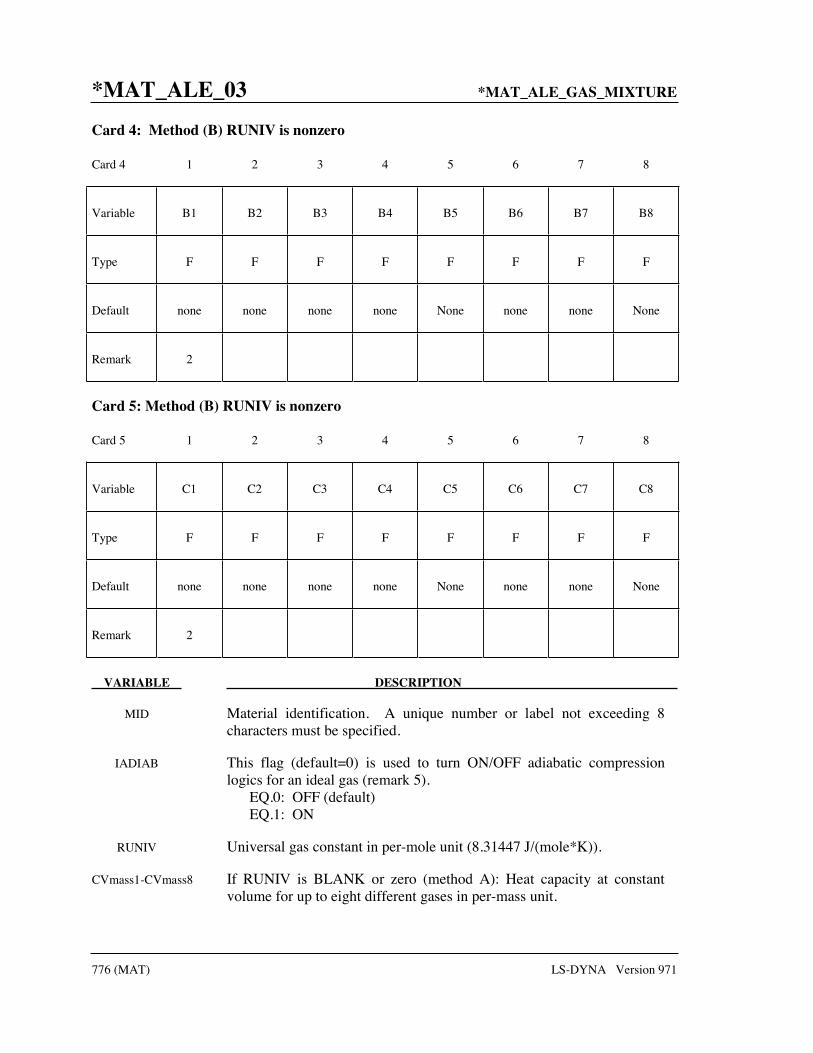
*MAT_ALE_03 *MAT_ALE_GAS_MIXTURE
776 (MAT) LS-DYNA Version 971
Card 4: Method (B) RUNIV is nonzero
Card 4 1 2 3 4 5 6 7 8
Variable B1 B2 B3 B4 B5 B6 B7 B8
Type F F F F F F F F
Default none none none none None none none None
Remark 2
Card 5: Method (B) RUNIV is nonzero
Card 5 1 2 3 4 5 6 7 8
Variable C1 C2 C3 C4 C5 C6 C7 C8
Type F F F F F F F F
Default none none none none None none none None
Remark 2
VARIABLE DESCRIPTION
MID Material identification. A unique number or label not exceeding 8 characters must be specified.
IADIAB This flag (default=0) is used to turn ON/OFF adiabatic compression logics for an ideal gas (remark 5).
EQ.0: OFF (default) EQ.1: ON
RUNIV Universal gas constant in per-mole unit (8.31447 J/(mole*K)).
CVmass1-CVmass8 If RUNIV is BLANK or zero (method A): Heat capacity at constant volume for up to eight different gases in per-mass unit.

*MAT_ALE_GAS_MIXTURE *MAT_ALE_03
LS-DYNA Version 971 777 (MAT)
VARIABLE DESCRIPTION
CPmass1-CPmass8 If RUNIV is BLANK or zero (method A): Heat capacity at constant pressure for up to eight different gases in per-mass unit.
MOLWT1-MOLWT8 If RUNIV is nonzero (method B): Molecular weight of each ideal gas in the mixture (mass-unit/mole).
CPmole1-CPmole8 If RUNIV is nonzero (method B): Heat capacity at constant pressure for up to eight different gases in per-mole unit. These are nominal heat capacity values typically at STP. These are denoted by the variable “A” in the equation in remark 2.
B1-B8 If RUNIV is nonzero (method B): First order coefficient for a temperature dependent heat capacity at constant pressure for up to eight different gases. These are denoted by the variable “B” in the equation in remark 2.
C1-C8 If RUNIV is nonzero (method B): Second order coefficient for a temperature dependent heat capacity at constant pressure for up to eight different gases. These are denoted by the variable “C” in the equation in remark 2.
Remarks:
1. There are 2 methods of defining the gas properties for the mixture. If RUNIV is BLANK or ZERO Method (A) is used to define constant heat capacities where per-mass unit values of Cv and Cp are input. Only cards 2 and 3 are required for this method. Method (B) is used to define constant or temperature dependent heat capacities where per-mole unit values of Cp are input. Cards 2-5 are required for this method.
2. The per-mass-unit, temperature-dependent, constant-pressure heat capacity is
2
0
[ * * ]( ) ~
*
~ ( * )
p
P
A B T C T JC T
MW kg K
A C J mole K
+ +=
=
2
3
~ ( * )
~ ( * )
B J mole K
C J mole K
The units shown are only for demonstration of the equation.
3. The initial temperature and the density of the gas species present in a mesh or part at time zero is specified by the keyword *INITIAL_GAS_MIXTURE.
4. The ideal gas mixture is assumed to be thermal equilibrium, that is, all species are at the same temperature (T). The gases in the mixture are also assumed to follow Dalton’s
Partial Pressure Law, =ngas
iiPP . The partial pressure of each gas is then TRP
igasii ρ=

*MAT_ALE_03 *MAT_ALE_GAS_MIXTURE
778 (MAT) LS-DYNA Version 971
where univgasi
RR
MW= . The individual gas species temperature equals the mixture
temperature. The temperature is computed from the internal energy where the mixture internal energy per unit volume is used,
i i
i
ngas ngas
V i V i i Vi i
Vi ngas
i Vi
e C T C T
eT T
C
ρ ρ
ρ
= =
= =
In general, the advection step conserves momentum and internal energy, but not kinetic energy. This can result in energy lost in the system and lead to a pressure drop. In *MAT_GAS_MIXTURE the dissipated kinetic energy is automatically stored in the internal energy. Thus in effect the total energy is conserved instead of conserving just the internal energy. This numerical scheme has been shown to improve accuracy in some cases. However, the user should always be vigilant and check the physics of the problem closely.
5. As an example consider an airbag surrounded by ambient air. As the inflator gas flows into the bag, the ALE elements cut by the airbag fabric shell elements will contain some inflator gas inside and some ambient air outside. The multi-material element treatment is not perfect. Consequently the temperature of the outside air may, occasionally, be made artificially high after the multi-material element treatment. To prevent the outside ambient air from getting artificially high T, set IDIAB=1 for the ambient air outside. Simple adiabatic compression equation is then assumed for the outside air. The use of this flag may be needed, but only when that outside air is modeled by the *MAT_GAS_MIXTURE card.
Example:
Consider a tank test model where the Lagrangian tank (Part S1) is surrounded by an ALE air mesh (Part H4=AMMGID 1). There are 2 ALE parts which are defined but initially have no corresponding mesh: part 5 (H5=AMMGID 2) is the resident gas inside the tank at t = 0, and part 6 (H6=AMMGID 2) is the inflator gas(es) which is injected into the tank when t > 0. AMMGID stands for ALE Multi-Material Group ID. Please see figure and input below. The *MAT_GAS_MIXTURE (MGM) card defines the gas properties of ALE parts H5 & H6. The MGM card input for both method (A) and (B) are shown.
The *INITIAL_GAS_MIXTURE card is also shown. It basically specifies that “AMMGID 2 may be present in part or mesh H4 at t=0, and the initial density of this gas is defined in the rho1 position which corresponds to the 1st material in the mixture (or H5, the resident gas).”

*MAT_ALE_GAS_MIXTURE *MAT_ALE_03
LS-DYNA Version 971 779 (MAT)
Example configuration:
Sample input:
$-------------------------------------------------------------------------------*PARTH5 = initial gas inside the tank $ PID SECID MID EOSID HGID GRAV ADPOPT TMID 5 5 5 0 5 0 0 *SECTION_SOLID 5 11 0 $-------------------------------------------------------------------------------$ Example 1: Constant heat capacities using per-mass unit. $*MAT_GAS_MIXTURE$ MID IADIAB R_univ $ 5 0 0$ Cv1_mas Cv2_mas Cv3_mas Cv4_mas Cv5_mas Cv6_mas Cv7_mas Cv8_mas $718.7828911237.56228$ Cp1_mas Cp2_mas Cp3_mas Cp4_mas Cp5_mas Cp6_mas Cp7_mas Cp8_mas $1007.00058 1606.1117 $-------------------------------------------------------------------------------$ Example 2: Variable heat capacities using per-mole unit. *MAT_GAS_MIXTURE$ MID IADIAB R_univ 5 0 8.314470 $ MW1 MW2 MW3 MW4 MW5 MW6 MW7 MW8 0.0288479 0.02256 $ Cp1_mol Cp2_mol Cp3_mol Cp4_mol Cp5_mol Cp6_mol Cp7_mol Cp8_mol 29.049852 36.23388 $ B1 B2 B3 B4 B5 B6 B7 B8 7.056E-3 0.132E-1 $ C1 C2 C3 C4 C5 C6 C7 C8 -1.225E-6 -0.190E-5 $-------------------------------------------------------------------------------$ One card is defined for each AMMG that will occupy some elements of a mesh set *INITIAL_GAS_MIXTURE$ SID STYPE MMGID T0 4 1 1 298.15 $ RHO1 RHO2 RHO3 RHO4 RHO5 RHO6 RHO7 RHO8 1.17913E-9*INITIAL_GAS_MIXTURE$ SID STYPE MMGID T0 4 1 2 298.15 $ RHO1 RHO2 RHO3 RHO4 RHO5 RHO6 RHO7 RHO8 1.17913E-9$-------------------------------------------------------------------------------
S1= tank
H4=AMMG1=background outside air (initially defined ALE mesh)
H5=AMMG2=initial gas inside the tank (this has no initial mesh)
H6=AMMG2=inflator gas(es) injected in (this has no initial mesh)
Cut-off view

*MAT_S01 *MAT_SPRING_ELASTIC
780 (MAT) LS-DYNA Version 971
*MAT_SPRING_ELASTIC
This is Material Type 1 for discrete springs and dampers. This provides a translational or rotational elastic spring located between two nodes. Only one degree of freedom is connected.
Card 1 1 2 3 4 5 6 7 8
Variable MID K
Type A8 F
VARIABLE DESCRIPTION
MID Material identification. A unique number or label not exceeding 8 characters must be specified.
K Elastic stiffness (force/displacement) or (moment/rotation).

*MAT_DAMPER_VISCOUS *MAT_S02
LS-DYNA Version 971 781 (MAT)
*MAT_DAMPER_VISCOUS
This is Material Type 2 for discrete springs and dampers. This material provides a linear translational or rotational damper located between two nodes. Only one degree of freedom is then connected.
Card 1 1 2 3 4 5 6 7 8
Variable MID DC
Type A8 F
VARIABLE DESCRIPTION
MID Material identification. A unique number or label not exceeding 8 characters must be specified.
DC Damping constant (force/displacement rate) or (moment/rotation rate).

*MAT_S03 *MAT_SPRING_ELASTOPLASTIC
782 (MAT) LS-DYNA Version 971
*MAT_SPRING_ELASTOPLASTIC
This is Material Type 3 for discrete springs and dampers. This material provides an elastoplastic translational or rotational spring with isotropic hardening located between two nodes. Only one degree of freedom is connected.
Card 1 1 2 3 4 5 6 7 8
Variable MID K KT FY
Type A8 F F F
VARIABLE DESCRIPTION
MID Material identification. A unique number or label not exceeding 8 characters must be specified.
K Elastic stiffness (force/displacement) or (moment/rotation).
KT Tangent stiffness (force/displacement) or (moment/rotation).
FY Yield (force) or (moment).

*MAT_SPRING_NONLINEAR_ELASTIC *MAT_S04
LS-DYNA Version 971 783 (MAT)
*MAT_SPRING_NONLINEAR_ELASTIC
This is Material Type 4 for discrete springs and dampers. This material provides a nonlinear elastic translational and rotational spring with arbitrary force versus displacement and moment versus rotation, respectively. Optionally, strain rate effects can be considered through a velocity dependent scale factor. With the spring located between two nodes, only one degree of freedom is connected.
Card 1 1 2 3 4 5 6 7 8
Variable MID LCD LCR
Type A8 I I
VARIABLE DESCRIPTION
MID Material identification. A unique number or label not exceeding 8 characters must be specified.
LCD Load curve ID describing force versus displacement or moment versus rotation relationship
LCR Optional load curve describing scale factor on force or moment as a function of relative velocity or. rotational velocity, respectively. The load curve must define the response in the negative and positive quadrants and pass through point (0,0).

*MAT_S05 *MAT_DAMPER_NONLINEAR_VISCOUS
784 (MAT) LS-DYNA Version 971
*MAT_DAMPER_NONLINEAR_VISCOUS
This is Material Type 5 for discrete springs and dampers. This material provides a viscous translational damper with an arbitrary force versus velocity dependency, or a rotational damper with an arbitrary moment versus rotational velocity dependency. With the damper located between two nodes, only one degree of freedom is connected.
Card 1 1 2 3 4 5 6 7 8
Variable MID LCDR
Type A8 I
VARIABLE DESCRIPTION
MID Material identification. A unique number or label not exceeding 8 characters must be specified.
LCDR Load curve identification describing force versus rate-of-displacement relationship or a moment versus rate-of-rotation relationship. The load curve must define the response in the negative and positive quadrants and pass through point (0,0).

*MAT_SPRING_GENERAL_NONLINEAR *MAT_S06
LS-DYNA Version 971 785 (MAT)
*MAT_SPRING_GENERAL_NONLINEAR
This is Material Type 6 for discrete springs and dampers. This material provides a general nonlinear translational or rotational spring with arbitrary loading and unloading definitions. Optionally, hardening or softening can be defined. With the spring located between two nodes, only one degree of freedom is connected.
Card 1 1 2 3 4 5 6 7 8
Variable MID LCDL LCDU BETA TYI CYI
Type A8 I I F F F
VARIABLE DESCRIPTION
MID Material identification. A unique number or label not exceeding 8 characters must be specified.
LCDL Load curve identification describing force/torque versus displacement/rotation relationship for loading, see Figure 126.1.
LCDU Load curve identification describing force/torque versus displacement/rotation relationship for unloading, see Figure 119.1.
BETA Hardening parameter, β: EQ.0.0: tensile and compressive yield with strain softening
(negative or zero slope allowed in the force versus displacement. load curves),
NE.0.0: kinematic hardening without strain softening, EQ.1.0: isotropic hardening without strain softening.
TYI Initial yield force in tension ( > 0)
CYI Initial yield force in compression ( < 0)
Remarks:
Load curve points are in the format (displacement, force or rotation, moment). The points must be in order starting with the most negative (compressive) displacement or rotation and ending with the most positive (tensile) value. The curves need not be symmetrical.
The displacement origin of the “unloading” curve is arbitrary, since it will be shifted as necessary as the element extends and contracts. On reverse yielding the “loading” curve will also be shifted along the displacement re or. rotation axis. The initial tensile and compressive yield forces (TYI and CYI) define a range within which the element remains elastic (i.e. the

*MAT_S06 *MAT_SPRING_GENERAL_NONLINEAR
786 (MAT) LS-DYNA Version 971
“loading” curve is used for both loading and unloading). If at any time the force in the element exceeds this range, the element is deemed to have yielded, and at all subsequent times the “unloading” curve is used for unloading.
Figure S06.1. General nonlinear material for discrete elements.

*MAT_SPRING_MAXWELL *MAT_S07
LS-DYNA Version 971 787 (MAT)
*MAT_SPRING_MAXWELL
This is Material Type 7 for discrete springs and dampers. This material provides a three Parameter Maxwell Viscoelastic translational or rotational spring. Optionally, a cutoff time with a remaining constant force/moment can be defined.
Card 1 1 2 3 4 5 6 7 8
Variable MID K0 KI BETA TC FC COPT
Type A8 F F F F F F
Default --- --- --- --- 1020 0 0
VARIABLE DESCRIPTION
MID Material identification. A unique number or label not exceeding 8 characters must be specified.
K0 K0, short time stiffness
KI K∞, long time stiffness
BETA Decay parameter.
TC Cut off time. After this time a constant force/moment is transmitted.
FC Force/moment after cutoff time
COPT Time implementation option: EQ.0: incremental time change, NE.0: continuous time change.
Remarks:
The time varying stiffness K(t) may be described in terms of the input parameters as
0( ) ( ) tK t K K K e β−∞ ∞= + − .
This equation was implemented by Schwer [1991] as either a continuous function of time or incrementally following the approach of Herrmann and Peterson [1968]. The continuous function of time implementation has the disadvantage of the energy absorber’s resistance decaying with increasing time even without deformation. The advantage of the incremental

*MAT_S07 *MAT_SPRING_MAXWELL
788 (MAT) LS-DYNA Version 971
implementation is that an energy absorber must undergo some deformation before its resistance decays, i.e., there is no decay until impact, even in delayed impacts. The disadvantage of the incremental implementation is that very rapid decreases in resistance cannot be easily matched.

*MAT_SPRING_INELASTIC *MAT_S08
LS-DYNA Version 971 789 (MAT)
*MAT_SPRING_INELASTIC
This is Material Type 8 for discrete springs and dampers. This material provides an inelastic tension or compression only, translational or rotational spring. Optionally, a user-specified unloading stiffness can be taken instead of the maximum loading stiffness.
Card 1 1 2 3 4 5 6 7 8
Variable MID LCFD KU CTF
Type A8 I F F
VARIABLE DESCRIPTION
MID Material identification. A unique number or label not exceeding 8 characters must be specified.
LCFD Load curve identification describing arbitrary force/torque versus displacement/rotation relationship. This curve must be defined in the positive force-displacement quadrant regardless of whether the spring acts in tension or compression.
KU Unloading stiffness (optional). The maximum of KU and the maximum loading stiffness in the force/displacement or the moment/rotation curve is used for unloading.
CTF Flag for compression/tension: EQ.-1.0: tension only, EQ.0.0: default is set to 1.0, EQ.1.0: compression only.

*MAT_S13 *MAT_SPRING_TRILINEAR_DEGRADING
790 (MAT) LS-DYNA Version 971
*MAT_SPRING_TRILINEAR_DEGRADING
This is Material Type 13 for discrete springs and dampers. This material allows concrete shearwalls to be modeled as discrete elements under applied seismic loading. It represents cracking of the concrete, yield of the reinforcement and overall failure. Under cyclic loading, the stiffness of the spring degrades but the strength does not.
Card 1 1 2 3 4 5 6 7 8
Variable MID DEFL1 F1 DEFL2 F2 DEFL3 F3 FFLAG
Type A8 F F F F F F F
VARIABLE DESCRIPTION
MID Material identification. A unique number or label not exceeding 8 characters must be specified.
DEFL1 Deflection at point where concrete cracking occurs.
F1 Force corresponding to DEFL1
DEFL2 Deflection at point where reinforcement yields
F2 Force corresponding to DEFL2
DEFL3 Deflection at complete failure
F3 Force corresponding to DEFL3
FFLAG Failure flag.

*MAT_SPRING_SQUAT_SHEARWALL *MAT_S14
LS-DYNA Version 971 791 (MAT)
*MAT_SPRING_SQUAT_SHEARWALL
This is Material Type 14 for discrete springs and dampers. This material allows squat shear walls to be modeled using discrete elements. The behavior model captures concrete cracking, reinforcement yield, ultimate strength followed by degradation of strength finally leading to collapse.
Card 1 1 2 3 4 5 6 7 8
Variable MID A14 B14 C14 D14 E14 LCID FSD
Type A8 F F F F F I F
VARIABLE DESCRIPTION
MID Material identification. A unique number or label not exceeding 8 characters must be specified.
A14 Material coefficient A
B14 Material coefficient B
C14 Material coefficient C
D14 Material coefficient D
E14 Material coefficient E
LCID Load curve ID referencing the maximum strength envelope curve
FSD Sustained strength reduction factor
Material coefficients A, B, C and D are empirically defined constants used to define the shape of the polynomial curves which govern the cyclic behavior of the discrete element. A different polynomial relationship is used to define the loading and unloading paths allowing energy absorption through hysteresis. Coefficient E is used in the definition of the path used to ‘jump’ from the loading path to the unloading path (or vice versa) where a full hysteresis loop is not completed. The load curve referenced is used to define the force displacement characteristics of the shear wall under monotonic loading. This curve is the basis to which the polynomials defining the cyclic behavior refer to. Finally, on the second and subsequent loading / unloading cycles, the shear wall will have reduced strength. The variable FSD is the sustained strength reduction factor.

*MAT_S15 *MAT_SPRING_MUSCLE
792 (MAT) LS-DYNA Version 971
*MAT_SPRING_MUSCLE
This is Material Type 15 for discrete springs and dampers. This material is a Hill-type muscle model with activation. It is for use with discrete elements. The LS-DYNA implementation is due to Dr. J.A. Weiss.
Card 1 1 2 3 4 5 6 7 8
Variable MID L0 VMAX SV A FMAX TL TV
Type A8 F F F F F F F
Default 1.0 1.0 1.0 1.0
Card 2
Variable FPE LMAX KSH
Type F F F
Default 0.0
VARIABLE DESCRIPTION
MID Material identification. A unique number or label not exceeding 8 characters must be specified.
L0 Initial muscle length, Lo.
VMAX Maximum CE shortening velocity, Vmax.
SV Scale factor, Sv, for Vmax vs. active state. LT.0: absolute value gives load curve ID GE.0: constant value of 1.0 is used
A Activation level vs. time function. LT.0: absolute value gives load curve ID GE.0: constant value of A is used
FMAX Peak isometric force, Fmax.

*MAT_SPRING_MUSCLE *MAT_S15
LS-DYNA Version 971 793 (MAT)
VARIABLE DESCRIPTION
TL Active tension vs. length function. LT.0: absolute value gives load curve ID GE.0: constant value of 1.0 is used
TV Active tension vs. velocity function. LT.0: absolute value gives load curve ID GE.0: constant value of 1.0 is used
FPE Force vs. length function, Fpe, for parallel elastic element. LT.0: absolute value gives load curve ID EQ.0: exponential function is used (see below) GT.0: constant value of 0.0 is used
LMAX Relative length when Fpe reaches Fmax. Required if Fpe=0 above.
KSH Constant, Ksh, governing the exponential rise of Fpe. Required if Fpe=0 above.
Remarks:
The material behavior of the muscle model is adapted from the original model proposed by Hill [1938]. Reviews of this model and extensions can be found in Winters [1990] and Zajac [1989]. The most basic Hill-type muscle model consists of a contractile element (CE) and a parallel elastic element (PE) (Figure 139.1). An additional series elastic element (SEE) can be added to represent tendon compliance. The main assumptions of the Hill model are that the contractile element is entirely stress free and freely distensible in the resting state, and is described exactly by Hill’s equation (or some variation). When the muscle is activated, the series and parallel elements are elastic, and the whole muscle is a simple combination of identical sarcomeres in series and parallel. The main criticism of Hill’s model is that the division of forces between the parallel elements and the division of extensions between the series elements is arbitrary, and cannot be made without introducing auxiliary hypotheses. However, these criticisms apply to any discrete element model. Despite these limitations, the Hill model has become extremely useful for modeling musculoskeletal dynamics, as illustrated by its widespread use today.
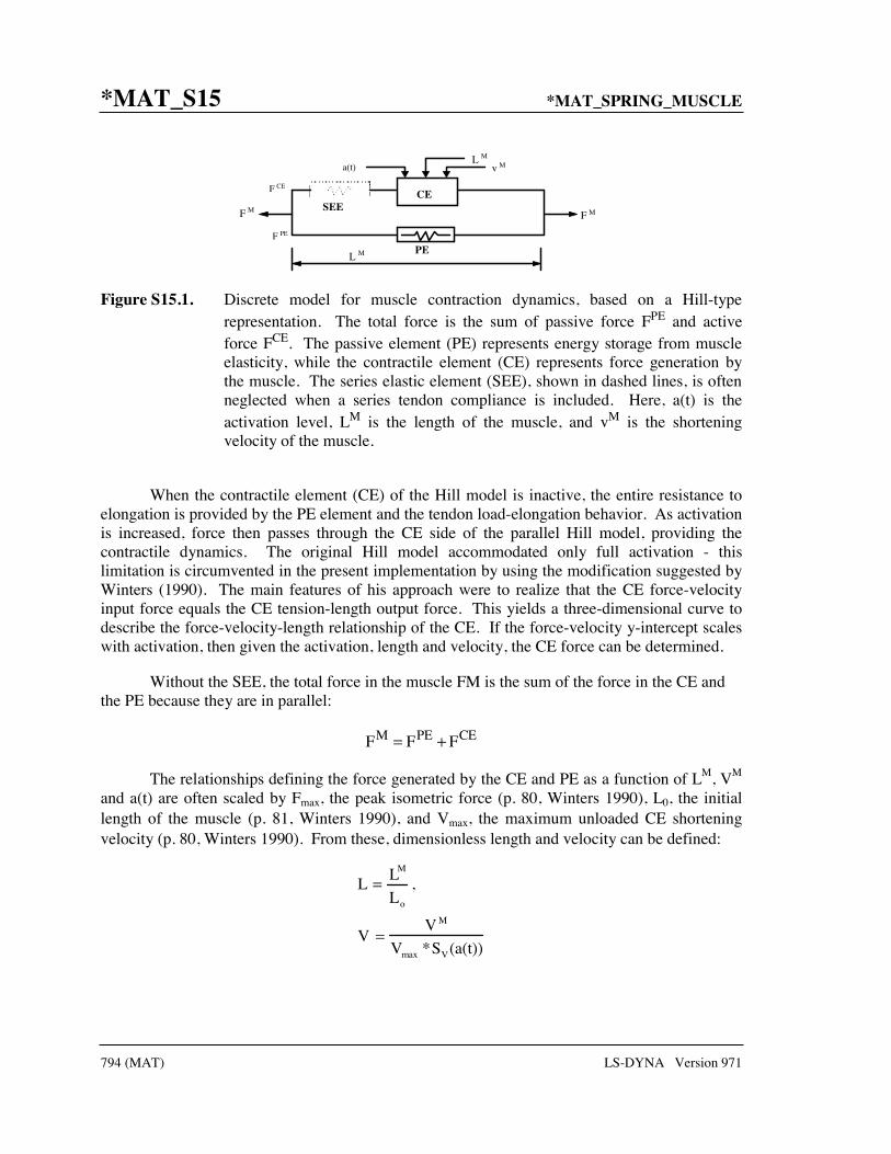
*MAT_S15 *MAT_SPRING_MUSCLE
794 (MAT) LS-DYNA Version 971
CE
a(t)L M
v M
F M
PE
SEEF M
F PE
F CE
L M
Figure S15.1. Discrete model for muscle contraction dynamics, based on a Hill-type representation. The total force is the sum of passive force FPE and active force FCE. The passive element (PE) represents energy storage from muscle elasticity, while the contractile element (CE) represents force generation by the muscle. The series elastic element (SEE), shown in dashed lines, is often neglected when a series tendon compliance is included. Here, a(t) is the activation level, LM is the length of the muscle, and vM is the shortening velocity of the muscle.
When the contractile element (CE) of the Hill model is inactive, the entire resistance to elongation is provided by the PE element and the tendon load-elongation behavior. As activation is increased, force then passes through the CE side of the parallel Hill model, providing the contractile dynamics. The original Hill model accommodated only full activation - this limitation is circumvented in the present implementation by using the modification suggested by Winters (1990). The main features of his approach were to realize that the CE force-velocity input force equals the CE tension-length output force. This yields a three-dimensional curve to describe the force-velocity-length relationship of the CE. If the force-velocity y-intercept scales with activation, then given the activation, length and velocity, the CE force can be determined.
Without the SEE, the total force in the muscle FM is the sum of the force in the CE and the PE because they are in parallel:
F F FM PE CE= +
The relationships defining the force generated by the CE and PE as a function of LM, VM
and a(t) are often scaled by Fmax, the peak isometric force (p. 80, Winters 1990), L0, the initial length of the muscle (p. 81, Winters 1990), and Vmax, the maximum unloaded CE shortening velocity (p. 80, Winters 1990). From these, dimensionless length and velocity can be defined:
L = LM
Lo
,
V =V M
Vmax *SV(a(t))

*MAT_SPRING_MUSCLE *MAT_S15
LS-DYNA Version 971 795 (MAT)
Here, SV scales the maximum CE shortening velocity Vmax and changes with activation level a(t). This has been suggested by several researchers, i.e. Winters and Stark [1985]. The activation level specifies the level of muscle stimulation as a function of time. Both have values between 0 and 1. The functions SV(a(t)) and a(t) are specified via load curves in LS-DYNA, or default values of SV=1 and a(t)=0 are used. Note that L is always positive and that V is positive for lengthening and negative for shortening.
The relationship between FCE, V and L was proposed by Bahler et al. [1967]. A three-dimensional relationship between these quantities is now considered standard for computer implementations of Hill-type muscle models [Winters 1990]. It can be written in dimensionless form as:
CEmax TL TVF a(t)*F *f (L)*f (V)=
Here, fTL and fTV are the tension-length and tension-velocity functions for active skeletal muscle.
Thus, if current values of LM, VM, and a(t) are known, then FCE can be determined (Figure 139.1).
The force in the parallel elastic element FPE is determined directly from the current length of the muscle using an exponential relationship [Winters 1990]:
( ) ( )
PE
PEMAX
PEsh
PEMAX sh max
Ff = 0, L 1
F
F 1 Kf = exp L 1 1 , L 1
F exp K 1 L
= ≤
= − − >−
Here, Lmax is the relative length at which the force Fmax occurs, and Ksh is a dimensionless shape parameter controlling the rate of rise of the exponential. Alternatively, the user can define a custom fPE curve giving tabular values of normalized force versus dimensionless length as a load curve.
For computation of the total force developed in the muscle FM, the functions for the tension-length fTL and force-velocity fTV relationships used in the Hill element must be defined. These relationships have been available for over 50 years, but have been refined to allow for behavior such as active lengthening. The active tension-length curve fTL describes the fact that isometric muscle force development is a function of length, with the maximum force occurring at an optimal length. According to Winters, this optimal length is typically around L=1.05, and the force drops off for shorter or longer lengths, approaching zero force for L=0.4 and L=1.5. Thus the curve has a bell-shape. Because of the variability in this curve between muscles, the user must specify the function fTL via a load curve, specifying pairs of points representing the normalized force (with values between 0 and 1) and normalized length L (Figure 163.1).

*MAT_S15 *MAT_SPRING_MUSCLE
796 (MAT) LS-DYNA Version 971
Figure S15.2. Typical normalized tension-length (TL) and tension-velocity (TV) curves for skeletal muscle.
The active tension-velocity relationship fTV used in the muscle model is mainly due to the original work of Hill. Note that the dimensionless velocity V is used. When V=0, the normalized tension is typically chosen to have a value of 1.0. When V is greater than or equal to 0, muscle lengthening occurs. As V increases, the function is typically designed so that the force increases from a value of 1.0 and asymptotes towards a value near 1.4. When V is less than zero, muscle shortening occurs and the classic Hill equation hyperbola is used to drop the normalized tension to 0 (Figure 163.1). The user must specify the function fTV via a load curve, specifying pairs of points representing the normalized tension (with values between 0 and 1) and normalized velocity V.

*MAT_SEATBELT *MAT_B01
LS-DYNA Version 971 797 (MAT)
*MAT_SEATBELT
Purpose: Define a seat belt material. See notes below.
Card 1 1 2 3 4 5 6 7 8
Variable MID MPUL LLCID ULCID LMIN
Type A8 F I I F
Default 0 0. 0 0 0.0
VARIABLE DESCRIPTION
MID Belt material number. A unique number or label not exceeding 8 characters must be specified.
MPUL Mass per unit length
LLCID Load curve identification for loading (force vs. engineering strain).
ULCID Load curve identification for unloading (force vs. engineering strain).
LMIN Minimum length (for elements connected to slip rings and retractors), see notes below.
CSE Optional compressive stress elimination option which applies to shell elements only (default 0.0):
EQ.0.0: eliminate compressive stresses in shell fabric EQ.1.0: don’t eliminate compressive stresses. This option should
not be used if retractors and sliprings are present in the model.
DAMP Optional Rayleigh damping coefficient, which applies to shell elements only. A coefficient value of 0.10 is the default corresponding to 10% of critical damping. Sometimes smaller or larger values work better.
Remarks:
Each belt material defines stretch characteristics and mass properties for a set of belt elements. The user enters a load curve for loading, the points of which are (Strain, Force). Strain is defined as engineering strain, i.e.
Strain =current length
initial length−1.

*MAT_B01 *MAT_SEATBELT
798 (MAT) LS-DYNA Version 971
Another similar curve is entered to describe the unloading behavior. Both load curves should start at the origin (0,0) and contain positive force and strain values only. The belt material is tension only with zero forces being generated whenever the strain becomes negative. The first non-zero point on the loading curve defines the initial yield point of the material. On unloading, the unloading curve is shifted along the strain axis until it crosses the loading curve at the ‘yield’ point from which unloading commences. If the initial yield has not yet been exceeded or if the origin of the (shifted) unloading curve is at negative strain, the original loading curves will be used for both loading and unloading. If the strain is less than the strain at the origin of the unloading curve, the belt is slack and no force is generated. Otherwise, forces will then be determined by the unloading curve for unloading and reloading until the strain again exceeds yield after which the loading curves will again be used.
A small amount of damping is automatically included. This reduces high frequency oscillation, but, with realistic force-strain input characteristics and loading rates, does not significantly alter the overall forces-strain performance. The damping forced opposes the relative motion of the nodes and is limited by stability:
.1 mass relativevelocityD
timestepsize
× ×=
In addition, the magnitude of the damping force is limited to one-tenth of the force calculated from the force-strain relationship and is zero when the belt is slack. Damping forces are not applied to elements attached to sliprings and retractors.
The user inputs a mass per unit length that is used to calculate nodal masses on initialization.
A ‘minimum length’ is also input. This controls the shortest length allowed in any element and determines when an element passes through sliprings or are absorbed into the retractors. One tenth of a typical initial element length is usually a good choice.

*MAT_THERMAL_OPTION *MAT
LS-DYNA Version 971 799 (MAT)
*MAT_THERMAL_OPTION
Available options include:
ISOTROPIC
ORTHOTROPIC
ISOTROPIC_TD
ORTHOTROPIC_TD
ISOTROPIC_PHASE_CHANGE
ISOTROPIC_TD_LC
The *MAT_THERMAL_ cards allow thermal properties to be defined in coupled structural/thermal and thermal only analyses, see *CONTROL_SOLUTION. Thermal properties must be defined for all solid and shell elements in such analyses. Thermal properties need not be defined for beam or discrete elements as these elements are not accounted for in the thermal phase of the calculation. However dummy thermal properties will be echoed for these elements in the D3HSP file.
Thermal material properties are specified by a thermal material ID number (TMID), this number is independent of the material ID number (MID) defined on all other *MAT_.. property cards. In the same analysis identical TMID and MID numbers may exist. The TMID and MID numbers are related through the *PART card.

*MAT_T01 *MAT_THERMAL_ISOTROPIC
800 (MAT) LS-DYNA Version 971
*MAT_THERMAL_ISOTROPIC
This is thermal material property type 1. It allows isotropic thermal properties to be defined.
Card (1 of 2)
Card 1 1 2 3 4 5 6 7 8
Variable TMID TRO TGRLC TGMULT TLAT HLAT
Type A8 F F F F F
Card (2 of 2)
Card 2 1 2 3 4 5 6 7 8
Variable HC TC
Type F F
VARIABLE DESCRIPTION
TMID Thermal material identification. A unique number or label not exceeding 8 characters must be specified.
TRO Thermal density: EQ 0.0 default to structural density.
TGRLC Thermal generation rate curve number, see *DEFINE_CURVE: GT.0: function versus time, EQ.0: use constant multiplier value, TGMULT, LT.0: function versus temperature.
TGMULT Thermal generation rate multiplier: EQ.0.0: no heat generation.
TLAT Phase change temperature
HLAT Latent heat
HC Heat capacity
TC Thermal conductivity

*MAT_THERMAL_ORTHOTROPIC *MAT_T02
LS-DYNA Version 971 801 (MAT)
*MAT_THERMAL_ORTHOTROPIC
This is thermal material property type 2. It allows orthotropic thermal properties to be defined.
Card (1 of 4)
Card 1 1 2 3 4 5 6 7 8
Variable TMID TRO TGRLC TGMULT AOPT TLAT HLAT
Type A8 F F F F F F
Card (2 of 4)
Card 2 1 2 3 4 5 6 7 8
Variable HC K1 K2 K3
Type F F F F
Card (3 of 4)
Card 3 1 2 3 4 5 6 7 8
Variable XP YP ZP A1 A2 A3
Type F F F F F F
Card (4 of 4)
Card 4 1 2 3 4 5 6 7 8
Variable D1 D2 D3
Type F F F

*MAT_T02 *MAT_THERMAL_ORTHOTROPIC
802 (MAT) LS-DYNA Version 971
VARIABLE DESCRIPTION
TMID Thermal material identification. A unique number or label not exceeding 8 characters must be specified.
TRO Thermal density: EQ 0.0 default to structural density.
TGRLC Thermal generation rate curve number, see *DEFINE_CURVE: GT.0: function versus time, EQ.0: use constant multiplier value, TGMULT, LT.0: function versus temperature.
TGMULT Thermal generation rate multiplier: EQ.0.0: no heat generation.
AOPT Material axes definition: EQ.0.0: locally orthotropic with material axes by element nodes
N1, N2 and N4, EQ.1.0: locally orthotropic with material axes determined by a
point in space and global location of element center, EQ.2.0: globally orthotropic with material axes determined by
vectors. LT.0.0: the absolute value of AOPT is a coordinate system ID
number (CID on *DEFINE_COORDINATE_NODES, *DEFINE_ COORDINATE_SYSTEM or *DEFINE_COORDINATE_ VECTOR). Available in R3 version of 971 and later.
TLAT Phase change temperature
HLAT Latent heat
HC Heat capacity
K1 Thermal conductivity K1 in local x-direction
K2 Thermal conductivity K2 in local y-direction
K3 Thermal conductivity K3 in local z-direction
XP, YP, ZP Define coordinate of point p for AOPT = 1
A1, A2, A3 Define components of vector a for AOPT = 2
D1, D2, D3 Define components of vector v for AOPT = 2

*MAT_THERMAL_ISOTROPIC_TD *MAT_T03
LS-DYNA Version 971 803 (MAT)
*MAT_THERMAL_ISOTROPIC_TD
This is thermal material property type 3. It allows temperature dependent isotropic properties to be defined. The temperature dependency is defined by specifying a minimum of two and a maximum of eight data points. The properties must be defined for the temperature range that the material will see in the analysis.
Card (1 of 4)
Card 1 1 2 3 4 5 6 7 8
Variable TMID TRO TGRLC TGMULT TLAT HLAT
Type A8 F F F F F
Card (2 of 4)
Card 2 1 2 3 4 5 6 7 8
Variable T1 T2 T3 T4 T5 T6 T7 T8
Type F F F F F F F F
Card (3 of 4)
Card 3 1 2 3 4 5 6 7 8
Variable C1 C2 C3 C4 C5 C6 C7 C8
Type F F F F F F F F
Card (4 of 4)
Card 4 1 2 3 4 5 6 7 8
Variable K1 K2 K3 K4 K5 K6 K7 K8
Type F F F F F F F F

*MAT_T03 *MAT_THERMAL_ISOTROPIC_TD
804 (MAT) LS-DYNA Version 971
VARIABLE DESCRIPTION
TMID Thermal material identification. A unique number or label not exceeding 8 characters must be specified.
TRO Thermal density: EQ 0.0 default to structural density.
TGRLC Thermal generation rate curve number, see *DEFINE_CURVE: GT.0: function versus time, EQ.0: use constant multiplier value, TGMULT, LT.0: function versus temperature.
TGMULT Thermal generation rate multiplier: EQ.0.0: no heat generation.
TLAT Phase change temperature
HLAT Latent heat
T1 ... T8 Temperatures (T1 ... T8)
C1 ... C8 Heat capacity at T1 ... T8
K1 ... K8 Thermal conductivity at T1 ... T8

*MAT_THERMAL_ORTHOTROPIC_TD *MAT_T04
LS-DYNA Version 971 805 (MAT)
*MAT_THERMAL_ORTHOTROPIC_TD
This is thermal material property type 4. It allows temperature dependent orthotropic properties to be defined. The temperature dependency is defined by specifying a minimum of two and a maximum of eight data points. The properties must be defined for the temperature range that the material will see in the analysis.
Card (1 of 8)
Card 1 1 2 3 4 5 6 7 8
Variable TMID TRO TGRLC TGMULT AOPT TLAT HLAT
Type A8 F F F F F F
Card (2 of 8)
Card 2 1 2 3 4 5 6 7 8
Variable T1 T2 T3 T4 T5 T6 T7 T8
Type F F F F F F F F
Card (3 of 8)
Card 3 1 2 3 4 5 6 7 8
Variable C1 C2 C3 C4 C5 C6 C7 C8
Type F F F F F F F F
Card (4 of 8)
Card 4 1 2 3 4 5 6 7 8
Variable (K1)1
(K1)2
(K1)3
(K1)4
(K1)5
(K1)6
(K1)7
(K1)8
Type F F F F F F F F

*MAT_T04 *MAT_THERMAL_ORTHOTROPIC_TD
806 (MAT) LS-DYNA Version 971
Card (5 of 8)
Card 5 1 2 3 4 5 6 7 8
Variable (K2)1
(K2)2
(K2)3
(K2)4
(K2)5
(K2)6
(K2)7
(K2)8
Type F F F F F F F F
Card (6 of 8)
Card 6 1 2 3 4 5 6 7 8
Variable (K3)1
(K3)2
(K3)3
(K3)4
(K3)5
(K3)6
(K3)7
(K3)8
Type F F F F F F F F
Card (7 of 8)
Card 7 1 2 3 4 5 6 7 8
Variable XP YP ZP A1 A2 A3
Type F F F F F F
Card (8 of 8)
Card 8 1 2 3 4 5 6 7 8
Variable D1 D2 D3
Type F F F
VARIABLE DESCRIPTION
TMID Thermal material identification. A unique number or label not exceeding 8 characters must be specified.
TRO Thermal density: EQ 0.0 default to structural density.

*MAT_THERMAL_ORTHOTROPIC_TD *MAT_T04
LS-DYNA Version 971 807 (MAT)
VARIABLE DESCRIPTION
TGRLC Thermal generation rate curve number, see *DEFINE_CURVE: GT.0: function versus time, EQ.0: use constant multiplier value, TGMULT, LT.0: function versus temperature.
TGMULT Thermal generation rate multiplier: EQ.0.0: no heat generation.
AOPT Material axes definition: (see Mat_OPTION TROPIC_ELASTIC for a more complete description):
EQ.0.0: locally orthotropic with material axes by element nodes N1, N2 and N4,
EQ.1.0: locally orthotropic with material axes determined by a point in space and global location of element center,
EQ.2.0: globally orthotropic with material axes determined by vectors.
TLAT Phase change temperature
HLAT Latent heat
T1 ... T8 Temperatures (T1 ... T8)
C1 ... C8 Heat capacity at T1 ... T8
(K1)1 ... (K1)8 Thermal conductivity K1 in local x-direction at T1 ... T8
(K2)1 ... (K2)8 Thermal conductivity K2 in local y-direction at T1 ... T8
(K3)1 ... (K3)8 Thermal conductivity K3 in local z-direction at T1 ... T8
XP, YP, ZP Define coordinate of point p for AOPT = 1
A1, A2, A3 Define components of vector a for AOPT = 2
D1, D2, D3 Define components of vector d for AOPT = 2

*MAT_T05 *MAT_THERMAL_ISOTROPIC_PHASE_CHANGE
808 (MAT) LS-DYNA Version 971
*MAT_THERMAL_ISOTROPIC_PHASE_CHANGE
This is thermal material property type 5. It allows temperature dependent isotropic properties with phase change to be defined. The latent heat of the material is defined together with the solid and liquid temperatures. The temperature dependency is defined by specifying a minimum of two and a maximum of eight data points. The properties must be defined for the temperature range that the material will see in the analysis.
Card (1 of 5)
Card 1 1 2 3 4 5 6 7 8
Variable TMID TRO TGRLC TGMULT
Type A8 F F F
Card (2 of 5)
Card 2 1 2 3 4 5 6 7 8
Variable T1 T2 T3 T4 T5 T6 T7 T8
Type F F F F F F F F
Card (3 of 5)
Card 3 1 2 3 4 5 6 7 8
Variable C1 C2 C3 C4 C5 C6 C7 C8
Type F F F F F F F F
Card (4 of 5)
Card 4 1 2 3 4 5 6 7 8
Variable K1 K2 K3 K4 K5 K6 K7 K8
Type F F F F F F F F

*MAT_THERMAL_ISOTROPIC_PHASE_CHANGE *MAT_T05
LS-DYNA Version 971 809 (MAT)
Card (5 of 5)
Card 5 1 2 3 4 5 6 7 8
Variable SOLT LIQT LH
Type F F F
VARIABLE DESCRIPTION
TMID Thermal material identification. A unique number or label not exceeding 8 characters must be specified.
TRO Thermal density: EQ 0.0 default to structural density.
TGRLC Thermal generation rate curve number, see *DEFINE_CURVE: GT.0: function versus time, EQ.0: use constant multiplier value, TGMULT, LT.0: function versus temperature.
TGMULT Thermal generation rate multiplier: EQ.0.0: no heat generation.
T1 ... T8 Temperatures (T1 ... T8)
C1 ... C8 Heat capacity at T1 ... T8
K1 ... K8 Thermal conductivity at T1 ... T8
SOLT Solid temperature, TS (must be < TL)
LIQT Liquid temperature, TL (must be > TS)
LH Latent heat
Remarks:
During phase change, that is between the solid and liquid temperatures, the heat capacity of the material will be enhanced to account for the latent heat as follows:
( ) 1 cos2 S
L S
T Tc t m
T Tπ −= −
− S LT T T< <

*MAT_T05 *MAT_THERMAL_ISOTROPIC_PHASE_CHANGE
810 (MAT) LS-DYNA Version 971
Where
TL = liquid temperature
TS = solid temperature
T = temperature
m = multiplier such that λ = C(T )dTTS
TL
λ = latent heat
c = heat capacity

*MAT_THERMAL_ISOTROPIC_TD_LC *MAT_T06
LS-DYNA Version 971 811 (MAT)
*MAT_THERMAL_ISOTROPIC_TD_LC
This is thermal material property type 6. It allows isotropic thermal properties that are temperature dependent specified by load curves to be defined. The properties must be defined for the temperature range that the material will see in the analysis.
Card (1 of 2)
Card 1 1 2 3 4 5 6 7 8
Variable TMID TRO TGRLC TGMULT
Type A8 F F F
Card (2 of 2)
Card 2 1 2 3 4 5 6 7 8
Variable HCLC TCLC
Type F F
VARIABLE DESCRIPTION
TMID Thermal material identification. A unique number or label not exceeding 8 characters must be specified.
TRO Thermal density: EQ 0.0 default to structural density.
TGRLC Thermal generation rate curve number, see *DEFINE_CURVE: GT.0: function versus time, EQ.0: use constant multiplier value, TGMULT, LT.0: function versus temperature.
TGMULT Thermal generation rate multiplier: EQ.0.0: no heat generation.
HCLC Load curve ID specifying heat capacity vs. temperature.
TCLC Load curve ID specifying thermal conductivity vs. temperature.

*MAT_T11 *MAT_THERMAL_USER_DEFINED
812 (MAT) LS-DYNA Version 971
*MAT_THERMAL_USER_DEFINED
These are Thermal Material Types 11-15. The user can supply his own subroutines. Please consult Appendix H for more information.
Card 1 1 2 3 4 5 6 7 8
Variable MID RO MT LMC NVH AOPT IORTHO IHVE
Type A8 F F F F F F F
Define the following two cards if and only if IORTHO=1
Card 2 1 2 3 4 5 6 7 8
Variable XP YP ZP A1 A2 A3
Type F F F F F F
Card 3
Variable D1 D2 D3
Type F F F
Define LMC material parameters using 8 parameters per card.
Card 4 1 2 3 4 5 6 7 8
Variable P1 P2 P3 P4 P5 P6 P7 P8
Type F F F F F F F F

*MAT_THERMAL_USER_DEFINED *MAT_T11
LS-DYNA Version 971 813 (MAT)
VARIABLE DESCRIPTION
MID Material identification. A unique number or label not exceeding 8 characters must be specified.
RO Thermal mass density.
MT User material type (11-15 inclusive).
LMC Length of material constants array. LMC must not be greater than 32.
NVH Number of history variables.
AOPT Material axes option of orthotropic materials. Use if IORTHO=1.0. EQ.0.0: locally orthotropic with material axes by element nodes
N1, N2 and N4, EQ.1.0: locally orthotropic with material axes determined by a
point in space and global location of element center, EQ.2.0: globally orthotropic with material axes determined by
vectors. LT.0.0: the absolute value of AOPT is a coordinate system ID
number (CID on *DEFINE_COORDINATE_NODES, *DEFINE_ COORDINATE_SYSTEM or *DEFINE_COORDINATE_ VECTOR). Available in R3 version of 971 and later.
IORTHO Set to 1.0 if the material is orthotropic.
IHVE Set to 1.0 to activate exchange of history variables between mechanical and thermal user material models.
XP-D3 Material axes orientation of orthotropic materials. Use if IORTHO=1.0 See *MAT_THERMAL_ORTHOTROPIC for a description.
P1 First material parameter. . . . .
PLMC LMCth material parameter.
Remarks:
1. The IHVE=1 option makes it possible for a thermal user material subroutine to read the history variables of a mechanical user material subroutine defined for the same part and vice versa. If the integration points for the thermal and mechanical elements are not coincident then extrapolation/interpolation is used to calculate the value when reading history variables.
2. Option _TITLE is supported
3. *INCLUDE_TRANSFORM: Transformation of units is only supported for RO field and vectors on card 2 and 3.

*MAT_T11 *MAT_THERMAL_USER_DEFINED
814 (MAT) LS-DYNA Version 971